SEISMIC TRAVELTIME TOMOGRAPHY OF THE CRUST … · · 2017-10-201 INTRODUCTION 2 recorded in such...
90
From: Advances in Geophysics, 46, 81-197. 1 SEISMIC TRAVELTIME TOMOGRAPHY OF THE CRUST AND LITHOSPHERE N. Rawlinson and M. Sambridge Research School of Earth Sciences, Australian National University, Canberra ACT 0200, Australia 1 Introduction 1.1 Motivation Seismic data represent one of the most valuable resources for investigating the internal structure and composition of the earth. One of the first people to deduce earth structure from seismic records was Mohoroviˇ ci´ c, a Serbian seismologist who, in 1909, observed two distinct traveltime curves from a regional earthquake. He determined that one curve corresponded to a direct crustal phase and the other to a wave refracted by a discontinuity in elastic properties between crust and upper mantle. This world-wide discontinuity is now known as the Mohoroviˇ ci´ c discontinuity or Moho for short. On a larger scale, the method of Herglotz and Wiechart (see, for example, Gubbins, 1992) was first implemented in 1910 to construct a 1-D whole earth model. The method uses the relationship between angular distance and ray parameter to determine velocity as a function of radius within the earth. Today, an abundance of methods exist for determining earth structure from seismic waves. Dif- ferent components of the seismic record may be used, including traveltimes, amplitudes, waveform spectra, full waveforms or the entire wavefield. Source-receiver configurations also differ - receiver arrays may be in-line or 3-D, sources may be close or distant to the receiver array, sources may be natural or artificial, and the scale of the study may be from tens of meters to the whole earth. Finally, there are a multitude of ways of translating the data extracted from the seismogram into a representation of seismic structure. The purpose of this article is to review a particular class of methods for imaging earth structure called seismic traveltime tomography. This is a form of seismic traveltime inversion that is used to constrain 2-D and 3-D models of the Earth represented by a significant number of parameters. The word tomography literally means slice picture (from the Greek word tomos meaning slice) and was first used in medical imaging to describe the process of mapping the internal density distribution of the human body using x-rays (Lee & Pereyra, 1993). The term was later appropriated by the seismological community to describe a similar process using seismic waves to map earth structure. Seismologists now routinely use tomography to refer to 3-D structural imaging even though, strictly speaking, the word was originally designed to describe the imaging of 2-D slices only. Inversion of source-receiver traveltimes of seismic waves is undoubtedly the most popular tech- nique for imaging subsurface structure at all scales. However, comprehensive up-to-date reviews of the methodology and their application are rarely found in the literature (some useful reference works include Nolet, 1987b; Iyer & Hirahara, 1993; Kennett, 1998). We hope to at least partially address this problem. Here, we restrict ourselves to traveltime tomography used in studies of the crust and lithosphere. These local scale studies typically involve the deployment of seismometer arrays with a spatial coverage of several hundred km or less in any dimension. The class of data that may be
Transcript of SEISMIC TRAVELTIME TOMOGRAPHY OF THE CRUST … · · 2017-10-201 INTRODUCTION 2 recorded in such...

From: Advances in Geophysics, 46, 81-197. 1
SEISMIC TRAVELTIME TOMOGRAPHY OF THECRUST AND LITHOSPHERE
N. Rawlinson and M. SambridgeResearch School of Earth Sciences, Australian National University,
Canberra ACT 0200, Australia
1 Introduction
1.1 Motivation
Seismic data represent one of the most valuable resources for investigating the internal structure andcomposition of the earth. One of the first people to deduce earth structure from seismic records wasMohorovicic, a Serbian seismologist who, in 1909, observed two distinct traveltime curves from aregional earthquake. He determined that one curve corresponded to a direct crustal phase and theother to a wave refracted by a discontinuity in elastic properties between crust and upper mantle.This world-wide discontinuity is now known as the Mohorovicic discontinuity or Moho for short.On a larger scale, the method of Herglotz and Wiechart (see, for example, Gubbins, 1992) wasfirst implemented in 1910 to construct a 1-D whole earth model. The method uses the relationshipbetween angular distance and ray parameter to determine velocity as a function of radius within theearth.
Today, an abundance of methods exist for determining earth structure from seismic waves. Dif-ferent components of the seismic record may be used, including traveltimes, amplitudes, waveformspectra, full waveforms or the entire wavefield. Source-receiver configurations also differ - receiverarrays may be in-line or 3-D, sources may be close or distant to the receiver array, sources maybe natural or artificial, and the scale of the study may be from tens of meters to the whole earth.Finally, there are a multitude of ways of translating the data extracted from the seismogram into arepresentation of seismic structure.
The purpose of this article is to review a particular class of methods for imaging earth structurecalled seismic traveltime tomography. This is a form of seismic traveltime inversion that is used toconstrain 2-D and 3-D models of the Earth represented by a significant number of parameters. Theword tomography literally means slice picture (from the Greek word tomos meaning slice) and wasfirst used in medical imaging to describe the process of mapping the internal density distributionof the human body using x-rays (Lee & Pereyra, 1993). The term was later appropriated by theseismological community to describe a similar process using seismic waves to map earth structure.Seismologists now routinely use tomography to refer to 3-D structural imaging even though, strictlyspeaking, the word was originally designed to describe the imaging of 2-D slices only.
Inversion of source-receiver traveltimes of seismic waves is undoubtedly the most popular tech-nique for imaging subsurface structure at all scales. However, comprehensive up-to-date reviews ofthe methodology and their application are rarely found in the literature (some useful reference worksinclude Nolet, 1987b; Iyer & Hirahara, 1993; Kennett, 1998). We hope to at least partially addressthis problem. Here, we restrict ourselves to traveltime tomography used in studies of the crust andlithosphere. These local scale studies typically involve the deployment of seismometer arrays witha spatial coverage of several hundred km or less in any dimension. The class of data that may be
1 INTRODUCTION 2
recorded in such experiments include normal incidence reflection, refraction and wide-angle reflec-tion, teleseismic and local earthquake arrival times. Although the inversion methods used in thesestudies are often common to a wide range of other seismic tomography applications, the point hereis that they are presented in the context of traveltime inversion for local-scale structure.
The widespread use of body wave traveltimes in seismic tomography is undoubtedly related tothe relative ease with which they may be extracted from a seismogram and the simple relationshipthat exists between traveltime and wavespeed. However, much more information is contained ina seismic waveform than simply the arrival time of a particular phase. Surface wave tomography,which utilizes the surface waveform component of an arriving wavetrain to build 3-D images of shearwavespeed, is the most commonly used type of waveform tomography. It is generally carried outat regional or global scales and has been particularly important in mapping beneath oceans (Nolet,1987a); oceanic upper mantle is rarely probed by body wave tomography since few seismic recordersare placed in an ocean setting. The methodology and application of surface wave tomography fallsoutside the scope of this review, so we refer the interested reader to the texts of Iyer & Hirahara(1993) and Kennett (2002) and the journal papers of Cara & Leveque (1987), Nolet (1990), Zielhuis& van der Hilst (1996) and Debayle & Kennett (2000) for more information on the subject.
This paper sets out to review commonly used methods of traveltime inversion for crustal andlithospheric imaging from the mid 1970s, when seismic tomography was first used, until recently,and provide a comprehensive list of references. However, we would like the paper to be morethan just a concatenation of method descriptions and a discussion of their relative merits. This isachieved in several ways. First, we impart a tutorial flavor to the paper by being instructive as wellas informative; this will be of particular benefit to readers who are not very familiar with seismictomography. For example, many schematic diagrams and technical drawings are included to try andillustrate basic concepts, or clarify important ideas. Second, recent techniques that have seen little orno application in seismic tomography but show significant potential are also explained (e.g. the fastmarching method of traveltime determination and global optimization techniques). Third, to helpunderstand how the various methods are used in real data applications, and how different classes ofdata influence the formulation of the inverse problem, we present a number of case studies in detail.Generally, these examples are very recent, although we also discuss earlier applications to emphasizehow the methodology has evolved. Lastly, we discuss in some detail the future of seismic traveltimetomography as a tool for subsurface imaging, and in particular the frontier areas of research thatremain to be explored.
In the remainder of this section, the basic concepts underlying seismic traveltime tomography areintroduced, and the four types of data for analyzing crustal and lithospheric structure are described(i.e. coincident reflection, refraction and wide-angle reflection, local earthquake and teleseismic). InSection 2, we review methods of seismic traveltime tomography, and in particular focus on modelparameterization, techniques for determining traveltimes, inversion schemes and practical methodsfor analyzing solution robustness. Application of these methods to each of the four data types arethen presented and compared in Section 3, with most examples taken from the existing literature.In Section 4, we conclude with a discussion on possible future developments in seismic traveltimetomography.
1.2 Seismic Traveltime Tomography: Formulation
If we represent some elastic property of the subsurface (e.g. velocity) by a set of model parametersm, then a set of data (e.g. traveltimes) d can be predicted for a given source-receiver array by line

1 INTRODUCTION 3
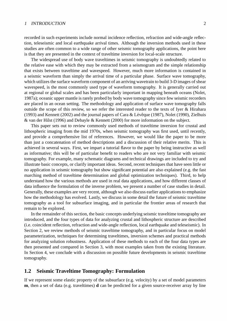
integration through the model. The relationship between data and model parameters, d = g(m),forms the basis of any tomographic method. For an observed dataset dobs and an initial model m0,the difference dobs −g(m0) gives an indication of how well the current model predictions satisfy thedata. The inverse problem in tomography is then to manipulate m in order to minimize the differencebetween observed and predicted data subject to any regularization that may be imposed. The endresult will be a mathematical representation of the true structure whose accuracy will depend on anumber of factors including: i) how well the observed data are satisfied by the model predictions, ii)assumptions made in parameterizing the model, iii) errors in the observed data, iv) accuracy of themethod for determining model predictions g(m), and v) the extent to which the data constrain themodel parameters. The tomographic method therefore depends implicitly on the general principlesof inverse theory (Tarantola, 1987; Menke, 1989; Parker, 1994) .
The steps required to produce a tomographic image from seismic data can thus be defined asfollows:
1. Model parameterization: The seismic structure of the region being mapped is defined interms of a set of unknown model parameters. Tomographic methods generally require aninitial estimate of model parameter values to be specified.
2. Forward calculation: A procedure is defined for the calculation of model data (e.g. travel-times) given a set of values for the model parameters.
3. Inversion: Automated adjustment of the model parameter values with the object of bettermatching the model data to the observed data subject to any regularization that may be im-posed.
4. Analysis of solution robustness: May be based on estimates of covariance and resolutionfrom linear theory or on the reconstruction of test models using synthetic datasets.
In seismic traveltime tomography the model data are traveltimes and the model parameters definevelocity variations. The traveltime of a ray in a continuous velocity medium v(x) is:
t =∫
L(v)
1
v(x)dl (1)
where L is the ray path and v(x) is the velocity field. Eq. 1 is non-linear since the integrationpath depends on the velocity. This inherent non-linearity means that the inverse problem can bevery difficult to solve. There are three basic approaches that are used, which we define as (i) lineartomography, (ii) iterative non-linear tomography, and (iii) fully non-linear tomography. In linear to-mography, the relationship between traveltime residual and velocity perturbation is linearized abouta reference model and corrections to the velocity field are made under this assumption. Thus, raypaths are determined only once (through the initial or reference model) and are not re-traced. It-erative non-linear tomography also ignores the path dependence of the velocity correction in theinversion step, but accounts for the non-linearity of the problem by iteratively applying correctionsand re-tracing rays (i.e. repeating steps 2 and 3 in the above formulation) until, for example, thedata are satisfied, or the rate of data fit improvement per iteration satisfies a given tolerance. Fullynon-linear tomography locates a solution without relying on linearization in any way, but is rarelydone in practice.
The linearization assumption commonly adopted in traveltime tomography is reasonable pro-vided it can be shown that the source-receiver path is not significantly perturbed by the adjustments

1 INTRODUCTION 4
made to the model parameter values in the inverse step. If we now consider a perturbation δv(x) toa reference velocity field v0(x), so that v(x) = v0(x) + δv(x), then both the ray path and source-receiver traveltime must also be perturbed in the new velocity field v(x) relative to v0(x). If the newpath is L(v) = L0 + δL where L0 is the path in v0(x) and t = t0 + δt where t0 is the traveltimealong L0 in v0(x), then the traveltime in v(x) can be written:
t =∫
L0+δL
1
v0 + δvdl (2)
The integrand in Eq. 2 may be expanded using the geometric series:
1
v0 + δv= 1/v0
1 − (−δv/v0)= 1
v0− δv
v20
+ δv2
v30
− . . . (3)
Substitution of this expression into Eq. 2 and ignoring second-order terms yields:
t =∫
L0+δL
1
v0− δv
v20
dl + O(δv2) (4)
which to first order may be separated as:
t =∫
L0
1
v0− δv
v20
dl +∫
δL
1
v0− δv
v20
dl + O(δv2) (5)
The second integral on the RHS can be set to zero since Fermat’s Principle states that, for fixedendpoints, the traveltime along a ray path is stationary with respect to perturbations in the path(∂ t/∂L = 0). Since t = t0 + δt , then the perturbation in traveltime resulting from a perturbation tothe velocity field is given by:
δt = −∫
L0
δv
v20
dl + O(δv2) (6)
The implication of Eq. 6 is that if the velocity along the path is perturbed, then the correspondingtraveltime perturbation calculated along the original path will be accurate to first order (see Snieder &Sambridge, 1993, for a discussion of the case in which ray end points are perturbed). It is interestingto note that if the above calculation is performed in terms of a perturbation in slowness s(x) = 1/v(x)rather than velocity, then the resulting expression for a perturbation in traveltime is given by:
δt =∫
L0
δsdl + O(δs2) (7)
which is linearly dependent on δs.Studies that use linear tomography may deal with tens to hundreds of thousands of model pa-
rameters (e.g. Inoue et al., 1990; Spakman, 1991; van der Hilst et al., 1997; Bijwaard et al., 1998),making an iterative non-linear approach computationally expensive, or have data geometries (suchas teleseismic) that make a linear assumption more valid (e.g. Achauer 1994). It is worth noting,however, that a number of recent regional and global scale traveltime tomography studies involv-ing hundreds of thousands to millions of ray paths and hundreds of thousands of model parametershave used iterative non-linear inversion schemes (Bijwaard & Spakman, 2000; Gorbatov et al., 2000,

1 INTRODUCTION 5
1
2
3
4
y
1 2 3 4
xFigure 1: Schematic representation of a source-receiver array (sources denoted by asterisks, receivers bytriangles) that bounds a model volume represented by a set of 16 constant velocity blocks labeled using(x, y) coordinates. Ray paths connect sources and receivers and demonstrate why the inverse problemoften requires regularization. Blocks (2,1) and (3,1) are not constrained by the data, blocks (1,1), (2,2),(3,2) and (4,1) are relatively poorly constrained by the data while blocks like (2,4) and (3,4) are relativelywell constrained by the data.
2001). Local earthquake and wide-angle tomography, for which ray paths depend strongly on ve-locity structure, generally use an iterative non-linear approach (e.g. Hole, 1992; Graeber & Asch,1999).
Common model parameterizations include constant velocity (or slowness) blocks, a grid of ve-locity nodes with a specified interpolant like trilinear or cubic splines, and to a lesser extent, spectralparameterizations like truncated Fourier series. Interface parameterizations use similar schemesexcept those appropriate to a surface rather than a volume. The forward problem of finding source-receiver ray paths and traveltimes is often solved using ray tracing techniques like shooting andbending, first-arrival wavefront tracking on a grid (e.g. eikonal solvers) and network methods, alsoknown as Shortest Path Raytracing (SPR). The inverse step of adjusting model parameters to sat-isfy observed data subject to regularization constraints is frequently solved using gradient methods(e.g. Gauss-Newton, subspace inversion) and backprojection methods like ART or SIRT. Globaloptimization methods like genetic algorithms (Goldberg, 1989) have been used but only rarely. Reg-ularization (i.e. applying other constraints to the model in addition to those supplied by the data) is animportant consideration in the inverse step due to the often under-determined or mixed-determinednature of the problem (see Fig. 1). A means of analyzing solution robustness is a critical step in ameaningful interpretation of an inversion result. Estimates of a posteriori model resolution and co-variance from linear theory have been used, as have synthetic reconstructions (e.g. the checkerboard
1 INTRODUCTION 6
test) that use the same source-receiver geometry as the original experiment. All the above methodsare discussed in more detail in Section 2.
Due to its origins in radiology and early seismic imaging, the term tomography is generallyonly applied to methods that invert for a property (e.g. velocity) that is described throughout themodel volume. If only interface structure is inverted for (e.g. Hole, 1992; Rawlinson & Houseman,1998), then the term tomography is generally not applied, even though the method conforms to theprocedures described above. However, in this paper we assume that the term tomography may beused for any method that generally follows the four steps listed above and results in 2-D or 3-Drepresentations of subsurface structure.
1.3 Traveltime Data used in Studies of the Crust and Lithosphere
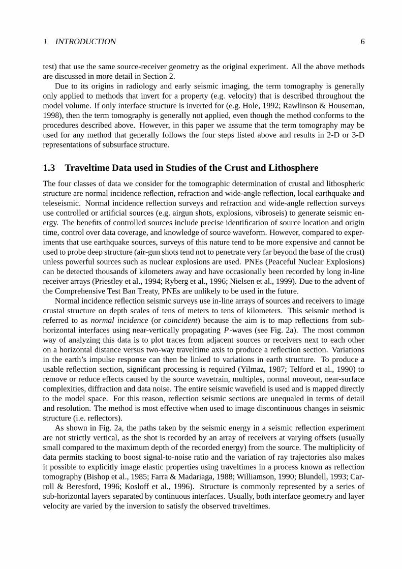
The four classes of data we consider for the tomographic determination of crustal and lithosphericstructure are normal incidence reflection, refraction and wide-angle reflection, local earthquake andteleseismic. Normal incidence reflection surveys and refraction and wide-angle reflection surveysuse controlled or artificial sources (e.g. airgun shots, explosions, vibroseis) to generate seismic en-ergy. The benefits of controlled sources include precise identification of source location and origintime, control over data coverage, and knowledge of source waveform. However, compared to exper-iments that use earthquake sources, surveys of this nature tend to be more expensive and cannot beused to probe deep structure (air-gun shots tend not to penetrate very far beyond the base of the crust)unless powerful sources such as nuclear explosions are used. PNEs (Peaceful Nuclear Explosions)can be detected thousands of kilometers away and have occasionally been recorded by long in-linereceiver arrays (Priestley et al., 1994; Ryberg et al., 1996; Nielsen et al., 1999). Due to the advent ofthe Comprehensive Test Ban Treaty, PNEs are unlikely to be used in the future.
Normal incidence reflection seismic surveys use in-line arrays of sources and receivers to imagecrustal structure on depth scales of tens of meters to tens of kilometers. This seismic method isreferred to as normal incidence (or coincident) because the aim is to map reflections from sub-horizontal interfaces using near-vertically propagating P-waves (see Fig. 2a). The most commonway of analyzing this data is to plot traces from adjacent sources or receivers next to each otheron a horizontal distance versus two-way traveltime axis to produce a reflection section. Variationsin the earth’s impulse response can then be linked to variations in earth structure. To produce ausable reflection section, significant processing is required (Yilmaz, 1987; Telford et al., 1990) toremove or reduce effects caused by the source wavetrain, multiples, normal moveout, near-surfacecomplexities, diffraction and data noise. The entire seismic wavefield is used and is mapped directlyto the model space. For this reason, reflection seismic sections are unequaled in terms of detailand resolution. The method is most effective when used to image discontinuous changes in seismicstructure (i.e. reflectors).
As shown in Fig. 2a, the paths taken by the seismic energy in a seismic reflection experimentare not strictly vertical, as the shot is recorded by an array of receivers at varying offsets (usuallysmall compared to the maximum depth of the recorded energy) from the source. The multiplicity ofdata permits stacking to boost signal-to-noise ratio and the variation of ray trajectories also makesit possible to explicitly image elastic properties using traveltimes in a process known as reflectiontomography (Bishop et al., 1985; Farra & Madariaga, 1988; Williamson, 1990; Blundell, 1993; Car-roll & Beresford, 1996; Kosloff et al., 1996). Structure is commonly represented by a series ofsub-horizontal layers separated by continuous interfaces. Usually, both interface geometry and layervelocity are varied by the inversion to satisfy the observed traveltimes.
1 INTRODUCTION 7
x
z x
z
x
zIncoming wavefront
x
z
(c) (d)
(a) (b)
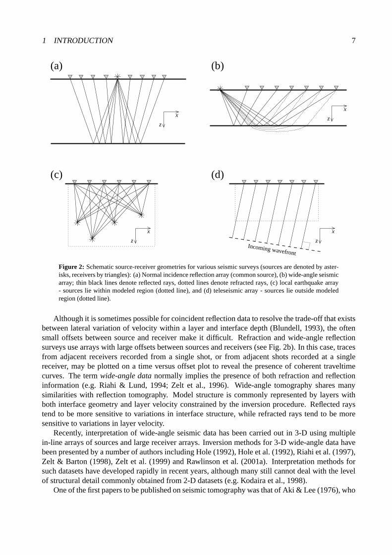
Figure 2: Schematic source-receiver geometries for various seismic surveys (sources are denoted by aster-isks, receivers by triangles): (a) Normal incidence reflection array (common source), (b) wide-angle seismicarray; thin black lines denote reflected rays, dotted lines denote refracted rays, (c) local earthquake array- sources lie within modeled region (dotted line), and (d) teleseismic array - sources lie outside modeledregion (dotted line).
Although it is sometimes possible for coincident reflection data to resolve the trade-off that existsbetween lateral variation of velocity within a layer and interface depth (Blundell, 1993), the oftensmall offsets between source and receiver make it difficult. Refraction and wide-angle reflectionsurveys use arrays with large offsets between sources and receivers (see Fig. 2b). In this case, tracesfrom adjacent receivers recorded from a single shot, or from adjacent shots recorded at a singlereceiver, may be plotted on a time versus offset plot to reveal the presence of coherent traveltimecurves. The term wide-angle data normally implies the presence of both refraction and reflectioninformation (e.g. Riahi & Lund, 1994; Zelt et al., 1996). Wide-angle tomography shares manysimilarities with reflection tomography. Model structure is commonly represented by layers withboth interface geometry and layer velocity constrained by the inversion procedure. Reflected raystend to be more sensitive to variations in interface structure, while refracted rays tend to be moresensitive to variations in layer velocity.
Recently, interpretation of wide-angle seismic data has been carried out in 3-D using multiplein-line arrays of sources and large receiver arrays. Inversion methods for 3-D wide-angle data havebeen presented by a number of authors including Hole (1992), Hole et al. (1992), Riahi et al. (1997),Zelt & Barton (1998), Zelt et al. (1999) and Rawlinson et al. (2001a). Interpretation methods forsuch datasets have developed rapidly in recent years, although many still cannot deal with the levelof structural detail commonly obtained from 2-D datasets (e.g. Kodaira et al., 1998).
One of the first papers to be published on seismic tomography was that of Aki & Lee (1976), who
1 INTRODUCTION 8
inverted first-arrival P-wave traveltimes from local earthquakes for velocity structure and hypocenterlocation in Bear Valley, California. The source-receiver geometry for this type of study is shownschematically in Fig. 2c - the earthquake sources lie beneath the receiver array within the modelvolume. The hypocenter coordinates, which are not accurately known, must be included in theinversion. Although Fig. 2c shows a 2-D experiment, most local earthquake studies are 3-D. Sincethe publication of the Aki & Lee (1976) paper, this branch of tomography has come into commonusage and is now popularly known as Local Earthquake Tomography or LET (Thurber, 1993).
LET has been used to image the lithosphere and upper asthenosphere to depths of up to 200 kmin subduction zone settings (Abers, 1994; Graeber & Asch, 1999). High resolution images of thecrust have also been obtained using shallow earthquakes (Thurber, 1983; Chiarabba et al., 1997). Insuch cases, the results of LET can be usefully compared with wide-angle studies of the same region(Eberhart-Phillips, 1990). Advantages of LET over wide-angle tomography include greater depthof penetration and the added structural information provided by the relocated hypocenters, e.g. theexistence of double seismic zones (Hasegawa et al., 1978; Kawakatsu, 1985; Kao & Rau, 1999).On the other hand, the relocation of hypocenters adds to the non-uniqueness of the solution andphases other than first-arrival P and S can be difficult to incorporate. For this reason, LET modelsrarely include interfaces, although Zhao et al. (1992) included interfaces in their LET model of NEJapan by using observed S P waves converted at the Moho and P S/S P waves converted at the upperboundary of the subducted Pacific Plate.
A significant difference between LET and teleseismic tomography is source location; in a tele-seismic study, earthquakes are generally thousands of km away from the receiver array. The targetregion of the crust and upper mantle lies beneath the receiver array. A key assumption of teleseismictomography is that only the region beneath the receiver array contains significant lateral variationsin velocity. Elsewhere, a 1-D earth model is adequate to predict the geometry and inclination of thewavefront before it strikes the target region. Therefore, it is possible to trace the rays through a 1-Dreference model of the earth until they penetrate the teleseismic model. Normally, relative traveltimeresiduals rather than absolute traveltimes are used in the inversion; this helps to account for errors inhypocenter location and large scale mantle heterogeneities. Fig. 2d shows a schematic diagram of awavefront from a distant earthquake incident on a teleseismic receiver array. As in LET, teleseismictomography is usually carried out in 3-D.
A seminal paper by Aki et al. (1977) used teleseismic data recorded at the Norsar array to invertfor velocity anomalies to a depth of 126 km. The final solution was produced by linear inversion.The assumption of linearity is more accurate in teleseismic tomography than in LET or wide-angleinversion. This occurs because the ray paths tend to be near-vertical as they transmit through themodel volume and hence are less affected by the dominant variations of velocity with depth. Con-sequently, many teleseismic tomography images, even those published recently, are the result oflinear inversions (Humphreys & Clayton, 1990; Glahn & Granet, 1993; Seber et al., 1996; Saltzer &Humphreys, 1997). If the traveltime residuals are suggestive of significant lateral structure, then aniterative non-linear approach may be required (Weiland et al., 1995; McQueen & Lambeck, 1996;Rawlinson & Houseman, 1998; Frederiksen et al., 1998; Steck et al., 1998; Graeber et al., 2002).
The main difficulties in teleseismic tomography arise because of the irregular and unpredictablenature of earthquakes. Earthquakes tend to occur at plate boundaries, so it is common to have a veryuneven distribution (in terms of azimuth and inclination) of ray paths through the target volume.Another factor is that relative traveltime residuals only provide good constraints on lateral variationsin velocity relative to an a priori lateral average. Vertical variations in the velocity field of the
2 METHODS OF TRAVELTIME INVERSION 9
solution model are poorly constrained and therefore must be interpreted with caution (Leveque &Masson, 1999).
The depth extent of teleseismic investigations may range from crustal (e.g. Lambeck et al., 1988;Rawlinson & Houseman, 1998) to many hundreds of kilometers (e.g. Humphreys & Clayton, 1990).The horizontal extent of the receiver array and the source distribution determines the depth to whichfeatures may be resolved. The vertical dimension of the model volume is often chosen on thisbasis, but it is always possible that structure outside the solution region causes some of the variationbetween traveltime residuals (e.g. Benz et al., 1992).
2 Methods of Traveltime Inversion
2.1 Representation of Structure
The traveltime of a seismic wave between source and receiver is solely dependent on the velocitystructure of the medium through which the wave propagates. Therefore, subsurface structure in aseismic traveltime inversion is represented by variations in P or S wave velocity (or slowness). Asmentioned in Section 1.2, velocity variations may be defined by a set of interfaces whose geometryis varied to satisfy the data, a set of constant velocity blocks or nodes with a specified interpolationfunction, or a combination of velocity and interface parameters. The most appropriate choice willdepend on the a priori information (e.g. known faults or other interfaces), whether or not the dataindicates the presence of interfaces (e.g. reflections, mode conversions), whether data coverage isadequate to resolve the trade-off between interface position and velocity, and finally, the capabilitiesof the inversion routine.
2.1.1 Velocity Parameterization
Constant velocity blocks (Fig. 3a) are simple to define and result in linear ray paths within eachblock. On the other hand, they are not a natural choice for representing smooth variations in subsur-face structure due to the velocity discontinuities that exist between adjacent blocks. These artificialdiscontinuities may also cause unwarranted ray shadow zones and triplications. However, if a largenumber of blocks are used and restrictions are placed on the size of the velocity changes betweenadjacent blocks, then a reasonable approximation to a continuously varying velocity field is possible.In teleseismic tomography, constant velocity blocks have been used by many authors including Akiet al. (1977), Oncescu et al. (1984), Humphreys & Clayton (1988), Humphreys & Clayton (1990),Benz et al. (1992), Achauer (1994) and Saltzer & Humphreys (1997). In wide-angle traveltimeinversions, the use of constant velocity blocks is not as common. Zhu & Ebel (1994) and Hilde-brand et al. (1989) use constant velocity blocks in the inversion of 3-D refraction traveltimes whileWilliamson (1990) and Blundell (1993) use them in an inversion of reflection traveltimes. Similarly,constant velocity blocks are only rarely used in local earthquake tomography (Aki & Lee, 1976;Nakanishi, 1985). This scheme for representing structure is often avoided when strong ray curvatureis expected.
An alternative to a block parameterization is to define velocities at the vertices of a rectangulargrid (see Fig. 3b) together with a specified interpolation function. One of the first examples of thisapproach was by Thurber (1983) in the context of local earthquake tomography. To describe thevelocity at any point (x, y, z) within a rectangular grid of nodes, he used a trilinear interpolation
2 METHODS OF TRAVELTIME INVERSION 10
1
9v8v7v
6v5v4v
v32vv
1
7
6
8
5
2
(b)(a) (c)
3 4
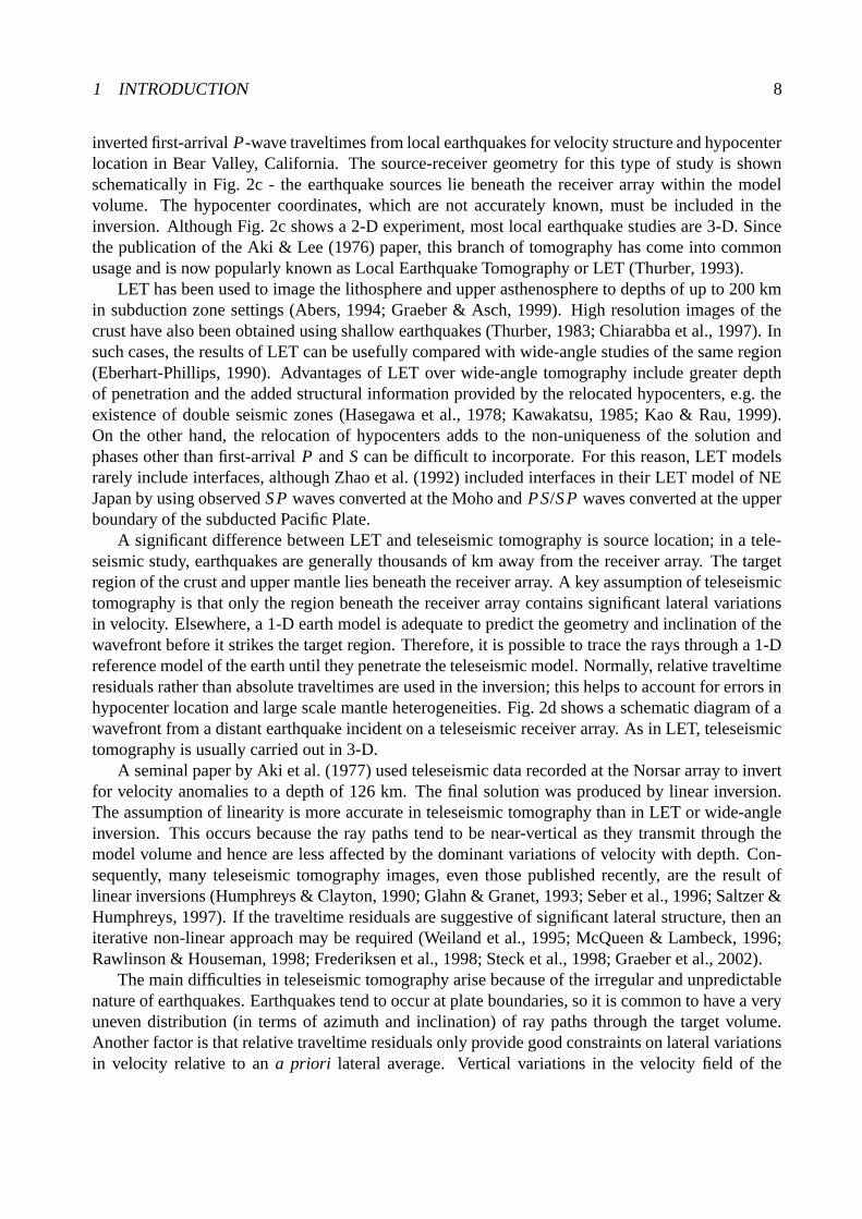
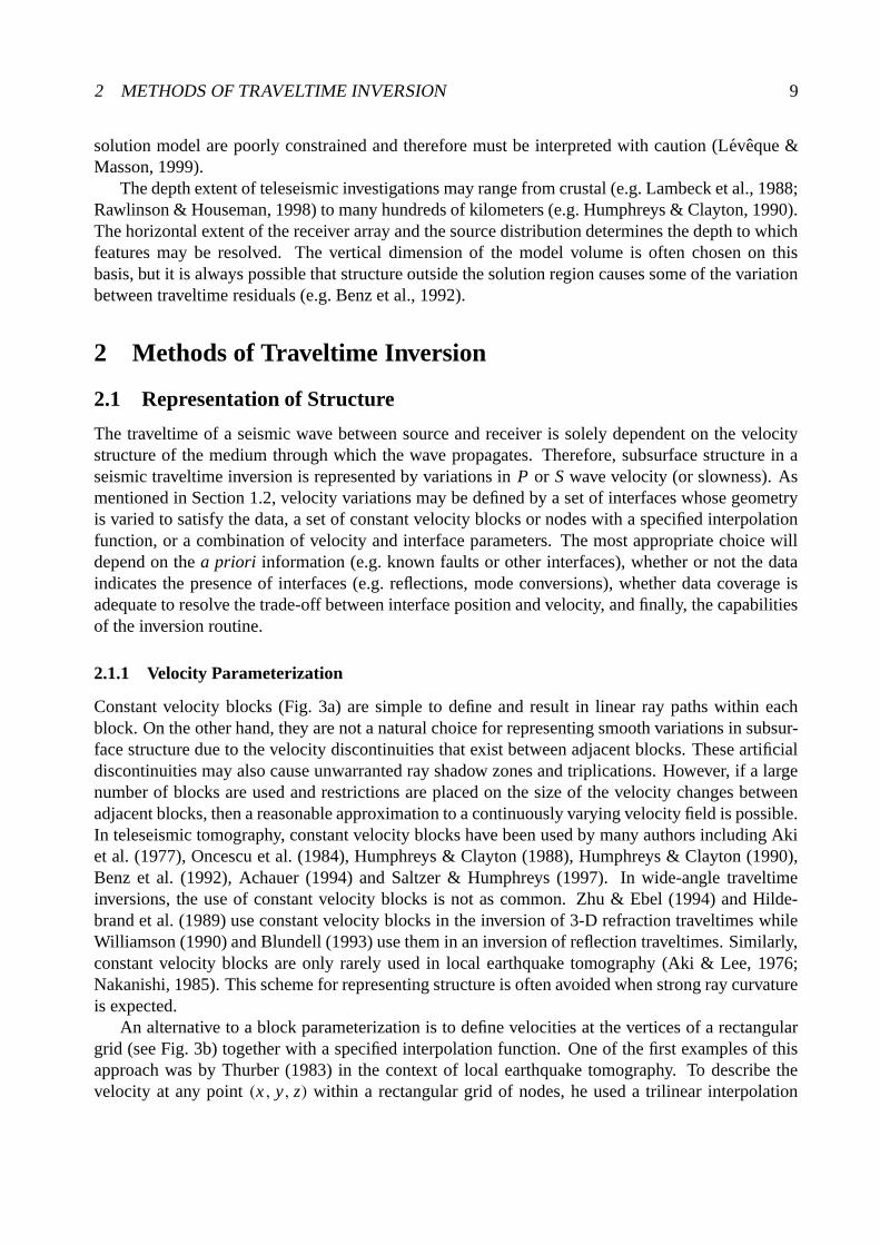
Figure 3: Different types of velocity parameterization: (a) constant velocity blocks, (b) a grid of velocitynodes, and (c) triangulated velocity grid designed for constant velocity gradient cells (after White, 1989).
function:
v(x, y, z) =2∑
i=1
2∑
j=1
2∑
k=1
V (xi , y j , zk)
(
1 −∣
∣
∣
∣
x − xi
x2 − x1
∣
∣
∣
∣
)(
1 −∣
∣
∣
∣
y − y j
y2 − y1
∣
∣
∣
∣
)(
1 −∣
∣
∣
∣
z − zk
z2 − z1
∣
∣
∣
∣
)
(8)
where V (xi , y j, zk) are the velocity values at the eight grid points surrounding (x, y, z). The useof Eq. 8 ensures that the velocity field will be continuous throughout the model volume, althoughthe velocity gradient will be discontinuous from cell to cell. This model parameterization is nowcommonly used in local earthquake tomography (Eberhart-Phillips, 1986, 1990; Zhao et al., 1992;Eberhart-Phillips & Michael, 1993; Scott et al., 1994; Haslinger et al., 1999), presumably becausemost of these inversions are based on the SIMULPS code devised by Thurber (1983). Zhao et al.(1994) and Steck et al. (1998) have used this parameterization in teleseismic tomography, althoughZhao et al. (1994) use a modified form of Eq. 8 for spherical coordinates.
Higher order interpolation functions must be used if the velocity field is to have continuous firstand second derivatives, which are required for some ray tracing methods (Thomson & Gubbins,1982). Cubic spline interpolation results in continuous first and second derivatives and has beenused by a number of authors. Thomson & Gubbins (1982), in a NORSAR teleseismic study, use thefollowing cubic spline function to describe the slowness field within a regular 3-D spherical grid ofnodes:
s(r, θ, φ) =4∑
i=1
4∑
j=1
4∑
k=1
Si j kCi (R)C j(2)Ck(8) (9)
where Si j k are the slowness values at the nodes of the 4 × 4 × 4 grid surrounding the point (r, θ, φ).Ci (R), C j (2) and Ck(8) are known as the cardinal splines (modified by Thomson & Gubbins,1982, for local support) and R, 2 and 8 are the local coordinates of r , θ and φ. Nodal valuesdo not necessarily equal the spline values at the node points. Sambridge (1990) uses a similarparameterization in Cartesian coordinates to describe a 3-D model constrained by traveltimes fromlocal earthquakes and explosions.
Cubic B-splines are similar to the cardinal splines described above in that they are locally sup-ported and do not necessarily pass through the node values. Conventional cubic spline interpolationforces the spline to pass through node values and is not locally supported. Undesirable effects of non-local support include poorly resolved portions of the model having a global influence and unrealisticvelocity fluctuations between nodes (Shalev, 1993). In 2-D wide-angle traveltime tomography, cubic
2 METHODS OF TRAVELTIME INVERSION 11
spline interpolation has been employed by Lutter et al. (1990), while Farra & Madariaga (1988) andMcCaughey & Singh (1997) have used cubic B-spline bases.
An interpolation method which features inherent flexibility is splines under tension (Smith &Wessel, 1990). Here, a tension factor is used to control the mode of interpolation, which, in the caseof Neele et al. (1993), can vary between near trilinear interpolation and cubic spline interpolation.The scheme features continuous first and second derivatives. Usually, one will choose a tensionfactor that results in a smooth model but minimizes unrealistic oscillations and maximizes localcontrol. Neele et al. (1993), VanDecar et al. (1995) and Ritsema et al. (1998) all use this approachin the inversion of teleseismic traveltimes.
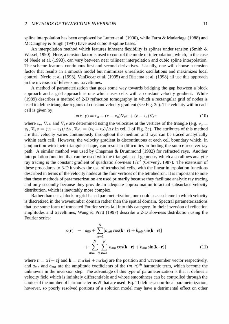
A method of parameterization that goes some way towards bridging the gap between a blockapproach and a grid approach is one which uses cells with a constant velocity gradient. White(1989) describes a method of 2-D refraction tomography in which a rectangular grid of nodes isused to define triangular regions of constant velocity gradient (see Fig. 3c). The velocity within eachcell is given by:
v(x, y) = vo + (x − xo)∇xv + (z − zo)∇zv (10)
where vo, ∇xv and ∇zv are determined using the velocities at the vertices of the triangle (e.g. vo =v1, ∇xv = (v2 − v1)/1x , ∇zv = (v5 − v2)/1z in cell 1 of Fig. 3c). The attributes of this methodare that velocity varies continuously throughout the medium and rays can be traced analyticallywithin each cell. However, the velocity gradient is discontinuous at each cell boundary which, inconjunction with their triangular shape, can result in difficulties in finding the source-receiver raypath. A similar method was used by Chapman & Drummond (1982) for refracted rays. Anotherinterpolation function that can be used with the triangular cell geometry which also allows analyticray tracing is the constant gradient of quadratic slowness 1/v2 (Cerveny, 1987). The extension ofthese procedures to 3-D involves the use of tetrahedral cells, with the linear interpolation functionsdescribed in terms of the velocity nodes at the four vertices of the tetrahedron. It is important to notethat these methods of parameterization are used primarily because they facilitate analytic ray tracingand only secondly because they provide an adequate approximation to actual subsurface velocitydistribution, which is inevitably more complex.
Rather than use a block or grid-based parameterization, one could use a scheme in which velocityis discretized in the wavenumber domain rather than the spatial domain. Spectral parameterizationsthat use some form of truncated Fourier series fall into this category. In their inversion of reflectionamplitudes and traveltimes, Wang & Pratt (1997) describe a 2-D slowness distribution using theFourier series:
s(r) = a00 +N∑
m=1
[am0 cos(k · r)+ bm0 sin(k · r)]
+N∑
m=−N
N∑
n=1
[amn cos(k · r)+ bmn sin(k · r)] (11)
where r = x i + zj and k = mπk0i + nπk0j are the position and wavenumber vector respectively,and amn and bmn are the amplitude coefficients of the (m, n)th harmonic term, which become theunknowns in the inversion step. The advantage of this type of parameterization is that it defines avelocity field which is infinitely differentiable and whose smoothness can be controlled through thechoice of the number of harmonic terms N that are used. Eq. 11 defines a non-local parameterization,however, so poorly resolved portions of a solution model may have a detrimental effect on other

2 METHODS OF TRAVELTIME INVERSION 12
regions of the model. Spectral parameterizations have been used in wide-angle traveltime inversionby Hildebrand et al. (1989), Hammer et al. (1994) and Wiggins et al. (1996) to study crustal structurebeneath deep oceans.
2.1.2 Including Interfaces
Velocity discontinuities are most commonly included in velocity models when the subsurface isrepresented by sub horizontal layers (see Fig. 4). In 2-D and 3-D traveltime inversion, the useof layered parameterizations has almost exclusively been the domain of reflection and refractiontomography. Reflection sections only image reflectors and refraction sections usually contain ob-vious later-arriving traveltime curves associated with velocity discontinuities. The issues related tochoosing an appropriate interface parameterization are similar to those for choosing an appropriatevelocity parameterization - representation of the geological structure and suitability for use in theforward and inverse solution steps.
x,z( )1v
v x,z( )2
v x,z( )3
v x,z( )4 zx
Figure 4: Schematic representation of the kind of layered velocity structure that can be imaged in reflectionand wide-angle traveltime inversion. The velocity functions vi (x, z) describe the velocity variation withina layer.
In 2-D, piecewise linear segments (see Fig. 5a) are probably the simplest means of representinginterface geometry. The wide-angle method of Zelt & Smith (1992) and the reflection method ofWilliamson (1990) employ this type of interface parameterization. One obvious problem with usingpiecewise linear segments is that the gradient of the interface is discontinuous at the joins betweensegments. Such discontinuity may not be geologically realistic and will create artificial shadow zonesbecause incident rays with very similar paths may depart from the interface along very different pathsif they intersect the interface on either side of a point of gradient discontinuity. Zelt & Smith (1992)avoid this problem by using an averaging filter to smooth the interface so that the departing ray hasa trajectory consistent with the smooth interface, but the point of projection is still given by theintersection point of the incident ray with the piecewise linear interface.
The logical extension of piecewise linear segments to a 3-D model with interface surfaces is

2 METHODS OF TRAVELTIME INVERSION 13
(a)
(b)
(c) (d)
Figure 5: Types of interface parameterization for 2-D (a-b) and 3-D (c-d) models. (a) Piecewise linearsegments, (b) piecewise cubic B-spline interpolation, (c) surface defined by mosaic of triangular patches,(d) surface defined by mosaic of bicubic B-spline patches - note that the surface is visualized here byorthogonal sets of lines.
to use piecewise triangular area segments (see Fig. 5c). Sambridge (1990) has used this approachin the inversion of local earthquake and quarry blast traveltimes. Guiziou et al. (1996) also used atriangulated interface structure in the tomographic inversion of reflection traveltimes in order to workwith geological models created in GOCAD (a computer aided design tool for modeling geologicalobjects). One advantage of triangulation is that multi-valued surfaces are easily described.
Analogous to defining velocity on a grid of nodes, an interface may be described by a grid ofdepth nodes with a specified interpolation function (piecewise linear segments can be viewed as aspecial case of this). Piecewise cubic spline functions with C2 continuity (see Fig. 5b) are com-monly used in wide-angle inversions. Conventional cubic splines have been used in a number of 2-Dschemes including those by White (1989), Lutter & Nowack (1990) and Rawlinson & Houseman(1998). Cerveny et al. (1984) parameterize a layered model with splines under tension for both in-terfaces and layer velocity fields. Cubic B-splines, which feature local control of interface geometry,have been used by Farra & Madariaga (1988) and McCaughey & Singh (1997). In 3-D, the use ofsmooth interfaces (see Fig. 5d) is less common, mainly because methods for the inversion of 3-Dlayered structures are less wide spread. The ray tracing method of Gjøystdal et al. (1984) param-eterizes interfaces in terms of bicubic splines, and the reflection tomography method of Chiu et al.(1986) describes interfaces using nth order polynomials (in practice, they use n ≤ 3). Like con-

2 METHODS OF TRAVELTIME INVERSION 14
tinuous velocity variations, interfaces are also amenable to spectral parameterization. For example,Wang & Houseman (1994) describe interfaces using a truncated Fourier series where the number ofharmonic terms controls the allowable flexibility of the interface. The problems associated with theuse of a global parameterization outlined above for velocity also apply to interface structure.
(a) x
z
(b)
2
x+b
x+b
v
2z=s
11
1
z=s
4v
2v
v3
Figure 6: Example of a layered structure parameterized using the method of Zelt & Smith (1992). (a)Structure composed of four layers with layer velocity defined by 25 velocity nodes (black squares) andinterface structure defined by 14 boundary nodes (grey circles). There is no velocity discontinuity betweenthe second and third layers and dashed lines indicate the lateral boundaries of trapezoids. (b) The velocityfield within a trapezoid is defined by interpolating between four corner values (grey triangles). If no velocitynode lies at a corner, then the required value is obtained by linear interpolation from adjacent nodes.
Irregular parameterizations are not very commonly used in traveltime tomography. However, ir-regular shaped elements can be adapted to suit variations in subsurface data coverage. The frequentlyused 2-D wide-angle inversion method of Zelt & Smith (1992) uses such a method. Layer bound-aries are described by a set of one or more arbitrarily spaced nodes interpolated linearly. Withineach layer, velocity nodes are specified on the upper and lower boundaries, the number and spacingof which may vary (Fig. 6a). To facilitate velocity interpolation, each layer is divided laterally intotrapezoidal blocks separated by vertical boundaries, which occur at each upper and lower boundarynode and velocity node. The velocity within each trapezoid is interpolated using the velocity valuesat the four corners (obtained by linear interpolation if a velocity node does not occupy a corner) suchthat the velocity within each layer varies linearly between the upper and lower boundaries in the ver-tical direction, and linearly along the upper and lower boundaries between nodes. Layer boundariesmay or may not represent velocity discontinuities. Fig. 6b shows the design of a trapezoid in moredetail. The velocity within a trapezoid is given by (Zelt & Smith, 1992):
v(x, z) = c1x + c2x2 + c3z + c4xz + c5
c6x + c7(12)
where {ci } are linear combinations of the corner velocities. The inherent flexibility of this techniquemeans that a velocity structure with or without layering can be represented. If layers are present,then it is possible for the velocity within the layers to vary arbitrarily.
Another example of irregular parameterization is given by Rawlinson et al. (2001a) in theirmethod of wide-angle traveltime inversion for 3-D layered crustal structure. They make use ofbicubic B-splines in parametric form to describe interface geometry. For a set of control vertices

2 METHODS OF TRAVELTIME INVERSION 15
(a) (b)
Figure 7: Flexibility of a cubic B-spline parameterization in parametric form. (a) Irregular grid of nodesdescribing a surface. Grey lines indicate surface patch boundaries. (b) Multivalued surface described bycubic B-splines.
pi, j = (xi, j , yi, j , zi, j) where i = 1, . . . ,m and j = 1, . . . , n, the B-spline for the i j th surface patchis:
BBBi, j(u, v) =2∑
k=−1
2∑
l=−1
bk(u)bl(v)pi+k, j+l (13)
so that any point on a surface patch is a function of two independent parameters u (0 ≤ u ≤ 1) andv (0 ≤ v ≤ 1). The weighting factors {bi} are the uniform cubic B-spline basis functions (Bartelset al., 1987). Properties of a surface constructed using a mosaic of B-spline patches defined byEq. 13 include C2 continuity and local control. Fig. 5d shows a bicubic B-spline surface describedby a regular grid of 16×16 vertices. In addition to inherent smoothness and local control, verticesmay lie on an irregular grid (Fig. 7a) and the surface may also be multivalued (Fig. 7b), althoughRawlinson et al. (2001a) did not make use of the latter property in their inversions. Control verticesmay be widely spaced in regions of poor data coverage and closely spaced in regions of good datacoverage.
Fault surfaces are another common feature of earth structure that may need to be represented ina model. Explicit representation of faults is not common in seismic methods. Faults are often near-vertical and cause discontinuities in the interfaces and velocity fields of sub-horizontal layers offsetby the fault. Ray-tracing through such a medium may be difficult and the inverse problem is likely tobe highly non-linear. Lambeck et al. (1988) and Lambeck & Burgess (1992) computed teleseismictraveltime residuals for a 2-D model in which constant velocity layers bounded by piecewise linearinterfaces were not required to be laterally continuous across the model, thus allowing faults to bedefined. Inversion of traveltime residuals was not attempted in either study, however. Wide-angleinversion methods that allow for complex lateral structure (e.g. Zelt & Smith, 1992) are usually notdesigned to represent faults. Laterally discontinuous structures like those found at subduction zones(Zelt, 1999) can be represented because interfaces tend to have a shallow dip and layer dislocationis not usually needed. Wang & Braile (1996), using a method based on that of Zelt & Smith (1992),represent faults implicitly by sharp near-vertical jumps in sub-horizontal interface structure in adja-

2 METHODS OF TRAVELTIME INVERSION 16
cent interfaces. However, these structures were constrained manually during the inversion process.When interfaces are used in conjunction with layer velocities specified by blocks or a grid of
nodes, then it is usually necessary to extrapolate the velocity field of each layer beyond the sur-rounding interfaces. These velocity parameters are redundant unless changes in interface geometrymade by the inversion step cause the relevant nodes to lie within the layer. The velocity within eachlayer is usually defined to be independent of velocities in other layers, so any spatial overlap of veloc-ity nodes from adjacent layers is of no consequence. In a 3-D wide-angle inversion study, Zelt et al.(1999) describe velocity structure using a continuous velocity parameterization but include “float-ing” reflectors. These floating reflectors allow reflections to be used to constrain interface structureand velocity but simplify traveltime determination by associating the reflectors with sharp gradientsin velocity rather than with velocity discontinuities.
As mentioned earlier, the use of interfaces in teleseismic traveltime tomography is rare. Zhaoet al. (1994) employ fixed interfaces described either by a power series or piecewise linear inter-polation in their simultaneous inversion of local, regional and teleseismic traveltimes for velocityvariation. Davis (1991) uses backprojection to invert teleseismic traveltime residuals for the struc-ture of the lithosphere-asthenosphere boundary in East Africa, defining interface geometry in termsof a polynomial expansion. Kohler & Davis (1997) use a similar procedure to determine 2-D crustalthickness variations in California from teleseismic traveltime residuals.
2.2 Traveltime Determination
The calculation of ray traveltimes between known end points through a given velocity structure isoften called the forward problem. When more than one ray path exists between a given sourceand receiver, the path with minimum traveltime is the one usually required because first-arrivalsare always easier to identify on a seismogram. Often, other quantities such as Frechet derivativesare calculated together with traveltime, but these parameters and their methods of computation aredescribed in the next section in the context of the relevant inversion method.
The traveltime of a seismic wave between source S and receiver R is given by the integral:
t =∫ R
S
1
v(x)dl (14)
where dl is differential path length, x is the position vector and v is velocity. The difficulty inperforming this integration, as pointed out in Section 1.2, is that the path taken by the seismicenergy depends on the velocity structure, and the path needs to be known in order to evaluate theintegral. For an elastic medium, the propagation of seismic wavefronts can be described by theeikonal equation:
(∇xT )2 = 1
[v(x)]2(15)
where T is the traveltime of the wavefront. This description of wave propagation is subject to theso-called high frequency assumption: the wavelength of a seismic wave should be much less thanthe length scale of the velocity variations of the medium through which it passes. If traveltime isdescribed by the equation T = T (x) and time is held constant, then TA = T (x) is an implicitequation for the wavefront at time TA (Aki & Richards, 1980). If TA is increased to, say, TB , thenthe equation TB = T (x) will describe the new geometry and position of the wavefront at a timeTB − TA later. If instead a point of constant phase on the wave is described as x = x(T ) then,
2 METHODS OF TRAVELTIME INVERSION 17
rather than implicitly describing a wavefront (i.e. a surface), we explicitly describe a ray path (i.e. acurve). Ray paths are by definition everywhere normal to wavefronts. The equation that governs thegeometry of ray paths can be derived from the eikonal equation by considering how a small changein time dt effects a point x on a wavefront (see Aki & Richards, 1980). The resultant ray equation:
d
dl
(
1
v(x)dxdl
)
= ∇(
1
v(x)
)
(16)
can be used to describe ray path geometry for any given velocity field v(x). A consequence of Eq. 16is Fermat’s principle - that of all the paths that join two points A and B in a velocity medium, thetrue ray path(s) will be stationary in time. In other words, the path along which the integral in Eq. 14is performed is one which extremizes t . This property was used to derive Eq. 6.
In traveltime tomography, the traditional means of determining source-receiver traveltimes is raytracing (Cerveny, 1987, 2001). More recently, wavefront tracking schemes such as finite differencesolutions of the eikonal equation have been employed (Vidale, 1988, 1990; Qin et al., 1992). An-other method that has seen recent application is network/graph theory, which makes direct use ofFermat’s principle (Nakanishi & Yamaguchi, 1986; Moser, 1991). Each of these methods of travel-time determination is described below.
2.2.1 Ray Tracing
The problem of finding a ray path between a source and receiver is a two point boundary valueproblem, for which there are two basic methods of solution: shooting and bending.
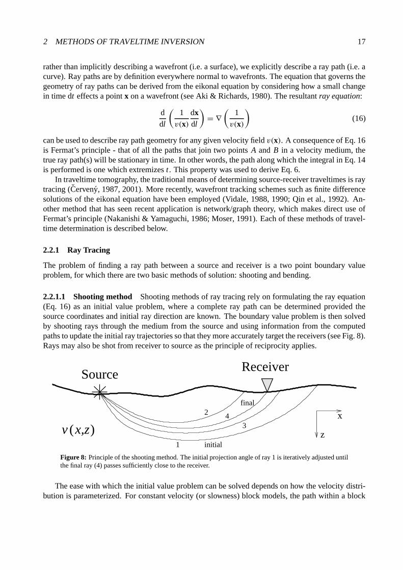
2.2.1.1 Shooting method Shooting methods of ray tracing rely on formulating the ray equation(Eq. 16) as an initial value problem, where a complete ray path can be determined provided thesource coordinates and initial ray direction are known. The boundary value problem is then solvedby shooting rays through the medium from the source and using information from the computedpaths to update the initial ray trajectories so that they more accurately target the receivers (see Fig. 8).Rays may also be shot from receiver to source as the principle of reciprocity applies.
SourceReceiver
v (x,z) z
x
final
initial1
43
2
Figure 8: Principle of the shooting method. The initial projection angle of ray 1 is iteratively adjusted untilthe final ray (4) passes sufficiently close to the receiver.
The ease with which the initial value problem can be solved depends on how the velocity distri-bution is parameterized. For constant velocity (or slowness) block models, the path within a block
2 METHODS OF TRAVELTIME INVERSION 18
is simply a straight line with traveltime varying linearly with distance. At cell boundaries, newtrajectories are calculated using Snell’s Law:
sin θi
vi= sin θr
vr(17)
where θi and θr are the angles of incident and refracted rays relative to the normal vector to theinterface, and vi and vr are the velocities of the media containing the incident and refracted raysrespectively.
Analytic ray tracing is also possible for media with a constant velocity gradient. Telford et al.(1976) derive parametric equations for ray path geometry and traveltime when velocity varies lin-early with depth z:
x = 1
pk(cos io − cos i)
z = 1
pk(sin i − sin io)
t = 1
kln
(
tan i2
tan io2
)
(18)
where i is the inclination of the ray (from the downgoing vertical), io is the initial inclination, k is thevelocity gradient and p is the ray parameter. When the velocity gradient is arbitrarily oriented, suchas when a grid of constant velocity gradient triangles or tetrahedra are used (see Section 2.1), thenthese expressions are modified by rotation of the coordinate system (White, 1989). Simple analyticsolutions are also possible when there is a constant gradient of quadratic slowness (see Cerveny,1987).
Only a few simple velocity functions allow for analytic solutions of the initial value problem. Forthe case of an arbitrary differentiable velocity function v(x), numerical solution of an initial valueformulation of the ray equation is required. For example, Zelt & Smith (1992), as part of their 2-Dwide-angle traveltime inversion method, solve two pairs of first-order differential equations:
dz
dx= cot θ
dθ
dx= vz − vx cot θ
v(19)
ordx
dz= tan θ
dθ
dz= vz tan θ − vx
v(20)
with initial conditions provided by source location (xo, zo) and ray take-off angle θo. θ is the angleof incidence (relative to the z-axis), vz = ∂v/∂z and vx = ∂v/∂x . Eq. 19 is used for near horizontalrays and Eq. 20 is used for near vertical rays. Both systems of equations are solved using a Runge-Kutta method with error control. Traveltime is determined by numerical integration of Eq. 14 usingthe trapezoidal rule. Sambridge & Kennett (1990) use the following set of equations to solve the
2 METHODS OF TRAVELTIME INVERSION 19
initial value problem in 3-D:
∂x
∂ t= v sin i cos j
∂y
∂ t= v sin i sin j
∂z
∂ t= v cos i
∂i
∂ t= − cos i
(
∂v
∂xcos j + ∂v
∂ysin j
)
+ ∂v
∂zsin i
∂ j
∂ t= 1
sin i
(
∂v
∂xsin j − ∂v
∂ycos j
)
(21)
where i and j represent the incidence angle and azimuth respectively of the ray. They also use aRunge-Kutta method to solve the system with the ray traveltime t as the integration variable. Theaccuracy of the ray path and associated traveltime determined via numerical ray tracing depends onthe accuracy of the solution scheme (4th order accurate in this case) and the length of the integrationstep.
wi
wr
wn
vi
vr
wr
Figure 9: At an interface, rays may refract and/or reflect. wi is tangent to the incident path, wr is tangentto the refracted (or reflected) path and wn is normal to the interface.
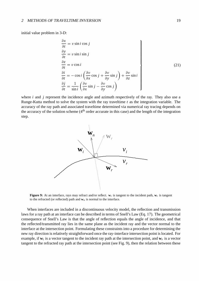
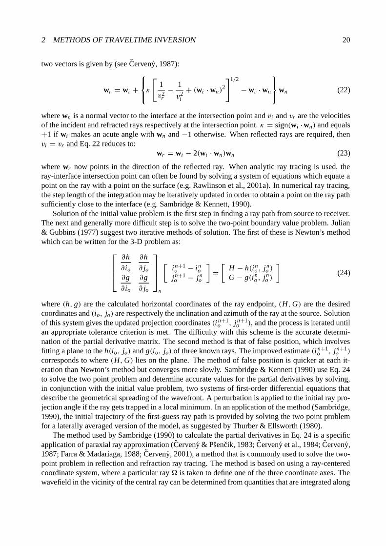
When interfaces are included in a discontinuous velocity model, the reflection and transmissionlaws for a ray path at an interface can be described in terms of Snell’s Law (Eq. 17). The geometricalconsequence of Snell’s Law is that the angle of reflection equals the angle of incidence, and thatthe reflected/transmitted ray lies in the same plane as the incident ray and the vector normal to theinterface at the intersection point. Formulating these constraints into a procedure for determining thenew ray direction is relatively straightforward once the ray-interface intersection point is located. Forexample, if wi is a vector tangent to the incident ray path at the intersection point, and wr is a vectortangent to the refracted ray path at the intersection point (see Fig. 9), then the relation between these
2 METHODS OF TRAVELTIME INVERSION 20
two vectors is given by (see Cerveny, 1987):
wr = wi +
κ
[
1
v2r
− 1
v2i
+ (wi · wn)2
]1/2
− wi · wn
wn (22)
where wn is a normal vector to the interface at the intersection point and vi and vr are the velocitiesof the incident and refracted rays respectively at the intersection point. κ = sign(wi · wn) and equals+1 if wi makes an acute angle with wn and −1 otherwise. When reflected rays are required, thenvi = vr and Eq. 22 reduces to:
wr = wi − 2(wi · wn)wn (23)
where wr now points in the direction of the reflected ray. When analytic ray tracing is used, theray-interface intersection point can often be found by solving a system of equations which equate apoint on the ray with a point on the surface (e.g. Rawlinson et al., 2001a). In numerical ray tracing,the step length of the integration may be iteratively updated in order to obtain a point on the ray pathsufficiently close to the interface (e.g. Sambridge & Kennett, 1990).
Solution of the initial value problem is the first step in finding a ray path from source to receiver.The next and generally more difficult step is to solve the two-point boundary value problem. Julian& Gubbins (1977) suggest two iterative methods of solution. The first of these is Newton’s methodwhich can be written for the 3-D problem as:
∂h
∂io
∂h
∂ jo∂g
∂io
∂g
∂ jo
n
[
in+1o − in
ojn+1o − jn
o
]
=[
H − h(ino , jn
o )
G − g(ino , jn
o )
]
(24)
where (h, g) are the calculated horizontal coordinates of the ray endpoint, (H,G) are the desiredcoordinates and (io, jo) are respectively the inclination and azimuth of the ray at the source. Solutionof this system gives the updated projection coordinates (i n+1
o , jn+1o ), and the process is iterated until
an appropriate tolerance criterion is met. The difficulty with this scheme is the accurate determi-nation of the partial derivative matrix. The second method is that of false position, which involvesfitting a plane to the h(io, jo) and g(io, jo) of three known rays. The improved estimate (i n+1
o , jn+1o )
corresponds to where (H,G) lies on the plane. The method of false position is quicker at each it-eration than Newton’s method but converges more slowly. Sambridge & Kennett (1990) use Eq. 24to solve the two point problem and determine accurate values for the partial derivatives by solving,in conjunction with the initial value problem, two systems of first-order differential equations thatdescribe the geometrical spreading of the wavefront. A perturbation is applied to the initial ray pro-jection angle if the ray gets trapped in a local minimum. In an application of the method (Sambridge,1990), the initial trajectory of the first-guess ray path is provided by solving the two point problemfor a laterally averaged version of the model, as suggested by Thurber & Ellsworth (1980).
The method used by Sambridge (1990) to calculate the partial derivatives in Eq. 24 is a specificapplication of paraxial ray approximation (Cerveny & Psencik, 1983; Cerveny et al., 1984; Cerveny,1987; Farra & Madariaga, 1988; Cerveny, 2001), a method that is commonly used to solve the two-point problem in reflection and refraction ray tracing. The method is based on using a ray-centeredcoordinate system, where a particular ray � is taken to define one of the three coordinate axes. Thewavefield in the vicinity of the central ray can be determined from quantities that are integrated along

2 METHODS OF TRAVELTIME INVERSION 21
the central ray using dynamic ray tracing. Geometric spreading and wavefront curvature parametersalong the initial ray � can be used to rapidly locate the two-point ray path from an initial ray that isnot too far from the target (see Cerveny et al., 1984).
Figure 10: Shooting method of Rawlinson et al. (2001a) used to find source-receiver refraction and reflec-tion ray paths.
In 2-D problems, a shooting approach is often used because the source-receiver array lies on asingle vertical plane, making the shooting of a single fan of rays an effective way of obtaining nearbyrays to all targets. Zelt & Smith (1992) use a bisection method to find rays that bound each requiredphase (e.g. a set of rays that all reflect back to the surface from a particular interface). The boundaryvalue problem is approximately solved by shooting a fan of rays into each defined region and linearlyinterpolating the required quantities between the two closest rays that bracket a receiver. Blundell(1993) uses a similar approach of shooting a fan of rays from the source to find 2-D reflection ar-rivals. The two-point problem is then solved using a secant algorithm or a bisection algorithm witha pair of rays that bracket the receiver. Similar methods were used by Cassell (1982) and Langanet al. (1985). Other applications of shooting methods in 2-D reflection and/or refraction traveltimeinversion include those by Farra & Madariaga (1988), White (1989), Lutter et al. (1990), Williamson(1990), Zelt & Smith (1992) and McCaughey & Singh (1997). Examples of its use in 3-D reflection
2 METHODS OF TRAVELTIME INVERSION 22
and/or refraction traveltime inversions are harder to find although several 3-D tomographic studiesthat combined refraction and local earthquake data (Benz & Smith, 1984; Ankeny et al., 1986; Sam-bridge, 1990) and some teleseismic tomography studies (Neele et al., 1993; VanDecar et al., 1995)have used shooting methods of ray tracing. Recently, Rawlinson et al. (2001a) developed a shootingmethod for finding refraction and reflection arrivals in 3-D layered media. Layer velocity varieslinearly with depth in their model, so they were able to analytically trace rays within layers usingequations similar to Eq. 18. The boundary value problem was solved using the Newton scheme ofEq. 24. Fig. 10 shows two-point paths through a 2-D layered model found using this method.
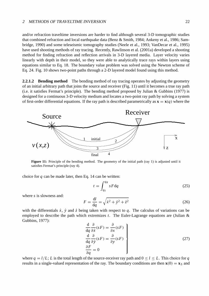
2.2.1.2 Bending method The bending method of ray tracing operates by adjusting the geometryof an initial arbitrary path that joins the source and receiver (Fig. 11) until it becomes a true ray path(i.e. it satisfies Fermat’s principle). The bending method proposed by Julian & Gubbins (1977) isdesigned for a continuous 3-D velocity medium and locates a two-point ray path by solving a systemof first-order differential equations. If the ray path is described parametrically as x = x(q) where the
SourceReceiver
v (x,z) z
xinitial
4
21
final
3
Figure 11: Principle of the bending method. The geometry of the initial path (ray 1) is adjusted until itsatisfies Fermat’s principle (ray 4).
choice for q can be made later, then Eq. 14 can be written:
t =∫ qR
qS
s Fdq (25)
where s is slowness and:
F = dl
dq=√
x2 + y2 + z2 (26)
with the differentials x , y and z being taken with respect to q. The calculus of variations can beemployed to describe the path which extremizes t . The Euler-Lagrange equations are (Julian &Gubbins, 1977):
d
dq
∂
∂ x(s F) = ∂
∂x(s F)
d
dq
∂
∂ y(s F) = ∂
∂y(s F)
∂F
∂q= 0
(27)
where q = l/L; L is the total length of the source-receiver ray path and 0 ≤ l ≤ L . This choice for qresults in a single-valued representation of the ray. The boundary conditions are then x(0) = xS and

2 METHODS OF TRAVELTIME INVERSION 23
x(1) = xR where xS and xR are the source and receiver coordinates respectively. These equationsare non-linear and cannot be solved directly. If some initial path x0(q) is chosen that passes throughS and R, then an improved estimate may be given by:
x1(q) = x0(q)+ ξξξ0(q) (28)
where ξξξ0(q) represents a perturbation to the initial path. If Eq. 28 is substituted into Eq. 27, then theresulting equations for ξξξ0 can be linearized and solved (see Julian & Gubbins, 1977), thus giving theimproved estimate x1. This process can be repeated until the solutions converge.
Pereyra et al. (1980) use a similar approach to locate two-point paths in arbitrary continuousmedia. They also extend their method to allow for the presence of interfaces. For a medium withan arbitrary number of interfaces that separate regions of smooth velocity variation, the bendingproblem can be treated by considering a separate system of non-linear differential equations in eachsmooth region. It is then possible to use the known discontinuity condition at each interface that istraversed by the ray to couple the separate systems. The disadvantage here is that the order in whichthe interfaces are traversed needs to be known in advance.
Um & Thurber (1987) develop a pseudo-bending technique for solving the two-point problemin continuous 3-D media. Their method is based on a perturbation scheme in which the integrationstep size is progressively halved. The initial guess path is defined by three points which are linearlyinterpolated. The center point is then iteratively perturbed using a geometric interpretation of theray equation until the traveltime extremum converges within a specified limit, at which point theray equation will be approximately satisfied. The number of path segments is then doubled and thethree-point perturbation scheme is repeated working from both endpoints to the middle (a total ofthree times for this step). The number of segments is doubled again and the procedure is repeatediteratively (see Fig. 12), until the change in traveltime between successive iterations satisfies someconvergence criterion.
SourceReceiver
v (x,z) z
xinitial
12
3final
Figure 12: Principle of the pseudo-bending method of Um & Thurber (1987). An initial guess ray definedby three points is provided. The center point is perturbed to best satisfy the ray equation. Then the number ofsegments is doubled and the process is repeated. This figure schematically represents three such iterations.
Compared to earlier bending methods, the pseudo-bending technique is much faster (Um &Thurber, 1987). Zhao et al. (1992) modify this technique to cope with interfaces as follows. Considertwo points A and B close to but on either side of an interface. Straight lines connect A and Bseparately to a point C on the interface. The correct ray-interface intersection point is obtained byadjusting the point C using a bisection method until Snell’s Law is satisfied.
2 METHODS OF TRAVELTIME INVERSION 24
Prothero et al. (1988) develop a 3-D bending method based on the simplex method of functionminimization. The first stage of the method is to locate the minimum-time circular path betweensource and receiver using an exhaustive search method. Perturbations to this path, described bya sum of sine wave harmonics, are then made using the simplex method which searches for theamplitude coefficients that produce the path of least time. The method is more robust than thepseudo-bending method of Um & Thurber (1987) but is significantly slower (Prothero et al., 1988).
Bending methods of ray tracing have been used by a number of authors in studies that invertteleseismic data (Thomson & Gubbins, 1982; Zhao et al., 1994, 1996; Steck et al., 1998), but notby many in the inversion of reflection or refraction data. Chiu et al. (1986) use a bending methodin the inversion of 3-D reflection traveltimes and Zhao et al. (1997) use the pseudo-bending methodin the inversion of refraction traveltimes for 2-D crustal structure. In local earthquake tomography,bending methods are probably most commonly used to find source-receiver paths and traveltimes(Eberhart-Phillips, 1990; Zhao et al., 1992; Scott et al., 1994; Eberhart-Phillips & Reyners, 1997;Graeber & Asch, 1999). In comparing their bending and shooting methods, Julian & Gubbins (1977)found that bending is computationally faster than shooting by a factor of 10 or more in media withcontinuous velocity variations. When discontinuities are present, however, the formulation of thebending problem becomes much more complex. In general, for smooth velocity structures that donot cause complex ray geometries, bending methods are more efficient, but when interfaces or strongvelocity gradients are present, shooting methods tend to be more robust and therefore preferable(Cerveny, 1987; Sambridge & Kennett, 1990).
The only other type of ray tracing scheme that is mentioned here is approximate ray tracing(Thurber & Ellsworth, 1980). Here, the velocity in a region local to the source and receiver islaterally averaged, and a 1-D ray tracer is used to find the minimum time-path through this laterallyinvariant structure. The resultant traveltime and path approximate the true first-arrival traveltimeand path through the 3-D model. If more accuracy is required, the ray path estimate can be used asa starting path in a bending routine (Thurber & Ellsworth, 1980). A variant of this technique wasintroduced by Thurber (1983), in which a large number of circular arcs with differing curvature anddip are joined between source and receiver. The traveltime along each arc is then computed usingthe 3-D velocity model. An approximation to the first-arrival ray is then selected by choosing thearc with minimum traveltime. Thurber (1983) and Eberhart-Phillips (1986) have used this style ofapproximate ray tracing in local earthquake tomography.
2.2.2 Wavefront Tracking
Rather than tracing rays from point to point through a medium to determine source-receiver travel-times, an alternative is to track the propagation path of the entire wavefront. The traveltime fromthe source to all points in the medium is found using this approach. The most common means ofwavefront tracking employs finite-difference solutions of the eikonal equation on a regular grid tocalculate the first-arrival traveltime field.
2.2.2.1 Finite difference schemes Vidale (1988) proposed a finite difference scheme that in-volves progressively integrating the traveltimes along an expanding square in 2-D. Strictly speaking,this method doesn’t track wavefronts to determine the traveltime field, but it represents a precursor
2 METHODS OF TRAVELTIME INVERSION 25
to the class of schemes that do, and is still widely used. The eikonal equation (Eq. 15) in 2-D is:
(
∂T
∂x
)2
+(
∂T
∂z
)2
= [s(x, z)]2 (29)
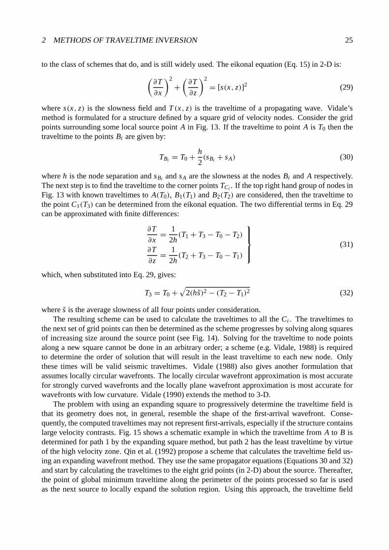
where s(x, z) is the slowness field and T (x, z) is the traveltime of a propagating wave. Vidale’smethod is formulated for a structure defined by a square grid of velocity nodes. Consider the gridpoints surrounding some local source point A in Fig. 13. If the traveltime to point A is T0 then thetraveltime to the points Bi are given by:
TBi = T0 + h
2(sBi + sA) (30)
where h is the node separation and sBi and sA are the slowness at the nodes Bi and A respectively.The next step is to find the traveltime to the corner points TCi . If the top right hand group of nodes inFig. 13 with known traveltimes to A(T0), B1(T1) and B2(T2) are considered, then the traveltime tothe point C1(T3) can be determined from the eikonal equation. The two differential terms in Eq. 29can be approximated with finite differences:
∂T
∂x= 1
2h(T1 + T3 − T0 − T2)
∂T
∂z= 1
2h(T2 + T3 − T0 − T1)
(31)
which, when substituted into Eq. 29, gives:
T3 = T0 +√
2(hs)2 − (T2 − T1)2 (32)
where s is the average slowness of all four points under consideration.The resulting scheme can be used to calculate the traveltimes to all the Ci . The traveltimes to
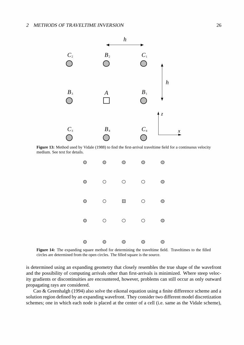
the next set of grid points can then be determined as the scheme progresses by solving along squaresof increasing size around the source point (see Fig. 14). Solving for the traveltime to node pointsalong a new square cannot be done in an arbitrary order; a scheme (e.g. Vidale, 1988) is requiredto determine the order of solution that will result in the least traveltime to each new node. Onlythese times will be valid seismic traveltimes. Vidale (1988) also gives another formulation thatassumes locally circular wavefronts. The locally circular wavefront approximation is most accuratefor strongly curved wavefronts and the locally plane wavefront approximation is most accurate forwavefronts with low curvature. Vidale (1990) extends the method to 3-D.
The problem with using an expanding square to progressively determine the traveltime field isthat its geometry does not, in general, resemble the shape of the first-arrival wavefront. Conse-quently, the computed traveltimes may not represent first-arrivals, especially if the structure containslarge velocity contrasts. Fig. 15 shows a schematic example in which the traveltime from A to B isdetermined for path 1 by the expanding square method, but path 2 has the least traveltime by virtueof the high velocity zone. Qin et al. (1992) propose a scheme that calculates the traveltime field us-ing an expanding wavefront method. They use the same propagator equations (Equations 30 and 32)and start by calculating the traveltimes to the eight grid points (in 2-D) about the source. Thereafter,the point of global minimum traveltime along the perimeter of the points processed so far is usedas the next source to locally expand the solution region. Using this approach, the traveltime field
2 METHODS OF TRAVELTIME INVERSION 26
A
C2
B3
C3 B4 C4
B1
C1B2
h
h
z
x
Figure 13: Method used by Vidale (1988) to find the first-arrival traveltime field for a continuous velocitymedium. See text for details.
Figure 14: The expanding square method for determining the traveltime field. Traveltimes to the filledcircles are determined from the open circles. The filled square is the source.
is determined using an expanding geometry that closely resembles the true shape of the wavefrontand the possibility of computing arrivals other than first-arrivals is minimized. Where steep veloc-ity gradients or discontinuities are encountered, however, problems can still occur as only outwardpropagating rays are considered.
Cao & Greenhalgh (1994) also solve the eikonal equation using a finite difference scheme and asolution region defined by an expanding wavefront. They consider two different model discretizationschemes; one in which each node is placed at the center of a cell (i.e. same as the Vidale scheme),
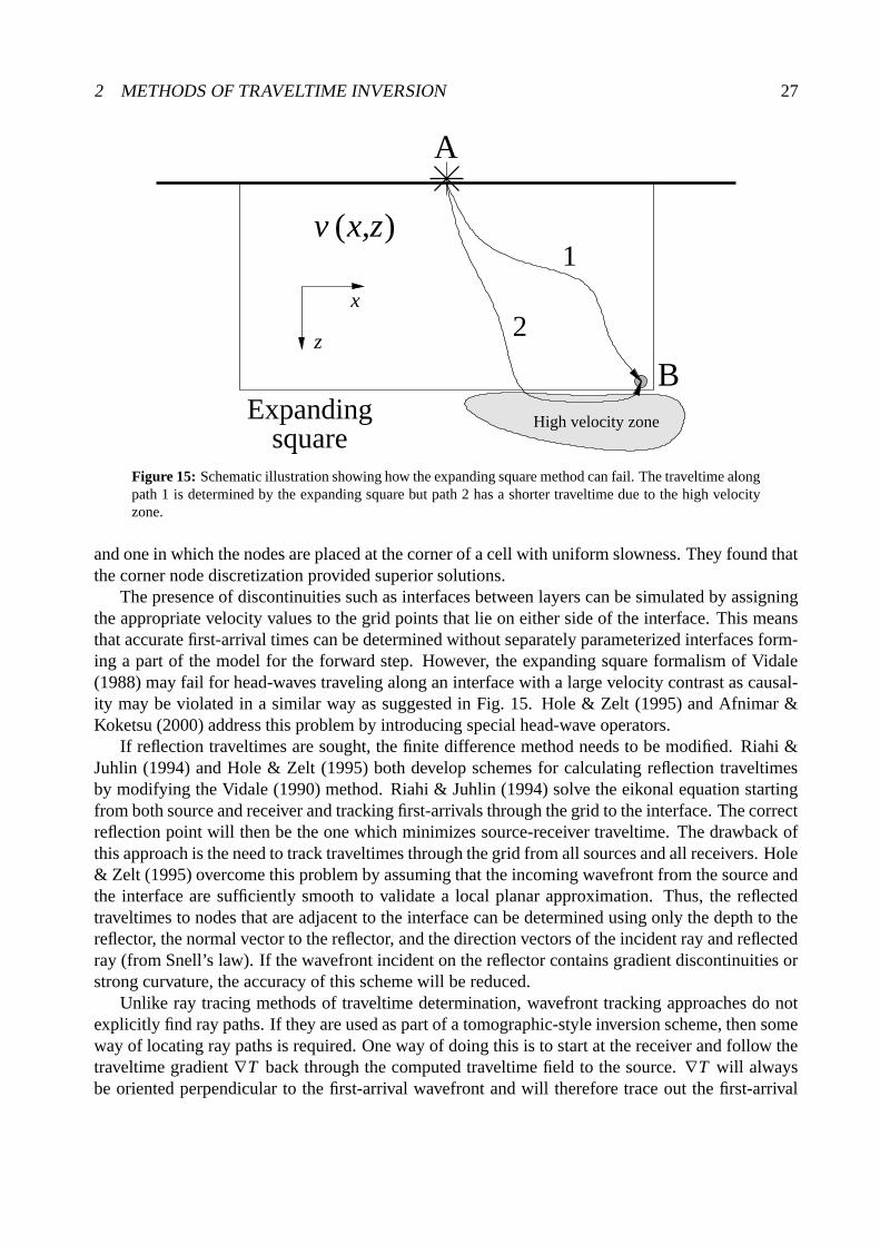
2 METHODS OF TRAVELTIME INVERSION 27
(x,z)v
BHigh velocity zone
1
A
2z
x
Expandingsquare
Figure 15: Schematic illustration showing how the expanding square method can fail. The traveltime alongpath 1 is determined by the expanding square but path 2 has a shorter traveltime due to the high velocityzone.
and one in which the nodes are placed at the corner of a cell with uniform slowness. They found thatthe corner node discretization provided superior solutions.
The presence of discontinuities such as interfaces between layers can be simulated by assigningthe appropriate velocity values to the grid points that lie on either side of the interface. This meansthat accurate first-arrival times can be determined without separately parameterized interfaces form-ing a part of the model for the forward step. However, the expanding square formalism of Vidale(1988) may fail for head-waves traveling along an interface with a large velocity contrast as causal-ity may be violated in a similar way as suggested in Fig. 15. Hole & Zelt (1995) and Afnimar &Koketsu (2000) address this problem by introducing special head-wave operators.
If reflection traveltimes are sought, the finite difference method needs to be modified. Riahi &Juhlin (1994) and Hole & Zelt (1995) both develop schemes for calculating reflection traveltimesby modifying the Vidale (1990) method. Riahi & Juhlin (1994) solve the eikonal equation startingfrom both source and receiver and tracking first-arrivals through the grid to the interface. The correctreflection point will then be the one which minimizes source-receiver traveltime. The drawback ofthis approach is the need to track traveltimes through the grid from all sources and all receivers. Hole& Zelt (1995) overcome this problem by assuming that the incoming wavefront from the source andthe interface are sufficiently smooth to validate a local planar approximation. Thus, the reflectedtraveltimes to nodes that are adjacent to the interface can be determined using only the depth to thereflector, the normal vector to the reflector, and the direction vectors of the incident ray and reflectedray (from Snell’s law). If the wavefront incident on the reflector contains gradient discontinuities orstrong curvature, the accuracy of this scheme will be reduced.
Unlike ray tracing methods of traveltime determination, wavefront tracking approaches do notexplicitly find ray paths. If they are used as part of a tomographic-style inversion scheme, then someway of locating ray paths is required. One way of doing this is to start at the receiver and follow thetraveltime gradient ∇T back through the computed traveltime field to the source. ∇T will alwaysbe oriented perpendicular to the first-arrival wavefront and will therefore trace out the first-arrival
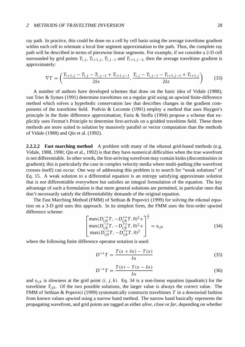
2 METHODS OF TRAVELTIME INVERSION 28
ray path. In practice, this could be done on a cell by cell basis using the average traveltime gradientwithin each cell to orientate a local line segment approximation to the path. Thus, the complete raypath will be described in terms of piecewise linear segments. For example, if we consider a 2-D cellsurrounded by grid points Ti, j , Ti+1, j , Ti, j−1 and Ti+1, j−1, then the average traveltime gradient isapproximately:
∇T =(
Ti+1, j − Ti, j − Ti, j−1 + Ti+1, j−1
2δx,
Ti, j − Ti, j−1 − Ti+1, j−1 + Ti+1, j
2δz
)
(33)
A number of authors have developed schemes that draw on the basic idea of Vidale (1988);van Trier & Symes (1991) determine traveltimes on a regular grid using an upwind finite-differencemethod which solves a hyperbolic conservation law that describes changes in the gradient com-ponents of the traveltime field. Podvin & Lecomte (1991) employ a method that uses Huygen’sprinciple in the finite difference approximation; Faria & Stoffa (1994) propose a scheme that ex-plicitly uses Fermat’s Principle to determine first-arrivals on a gridded traveltime field. These threemethods are more suited to solution by massively parallel or vector computation than the methodsof Vidale (1988) and Qin et al. (1992).
2.2.2.2 Fast marching method A problem with many of the eikonal grid-based methods (e.g.Vidale, 1988, 1990; Qin et al., 1992) is that they have numerical difficulties when the true wavefrontis not differentiable. In other words, the first-arriving wavefront may contain kinks (discontinuities ingradient); this is particularly the case in complex velocity media where multi-pathing (the wavefrontcrosses itself) can occur. One way of addressing this problem is to search for “weak solutions” ofEq. 15. A weak solution to a differential equation is an entropy satisfying approximate solutionthat is not differentiable everywhere but satisfies an integral formulation of the equation. The keyadvantage of such a formulation is that more general solutions are permitted, in particular ones thatdon’t necessarily satisfy the differentiability demands of the original equation.
The Fast Marching Method (FMM) of Sethian & Popovici (1999) for solving the eikonal equa-tion on a 3-D grid uses this approach. In its simplest form, the FMM uses the first-order upwinddifference scheme:
max(D−xi jk T ,−D+x
i jk T , 0)2+max(D−y
i jk T ,−D+yi jk T , 0)2+
max(D−zi jkT ,−D+z
i jkT , 0)2
12
= si j k (34)
where the following finite difference operator notation is used:
D+x T = T (x + δx)− T (x)
δx(35)
D−x T = T (x)− T (x − δx)
δx(36)
and si j k is slowness at the grid point (i, j, k). Eq. 34 is a non-linear equation (quadratic) for thetraveltime Ti j k. Of the two possible solutions, the larger value is always the correct value. TheFMM of Sethian & Popovici (1999) systematically constructs traveltimes T in a downwind fashionfrom known values upwind using a narrow band method. The narrow band basically represents thepropagating wavefront, and grid points are tagged as either alive, close or far, depending on whether
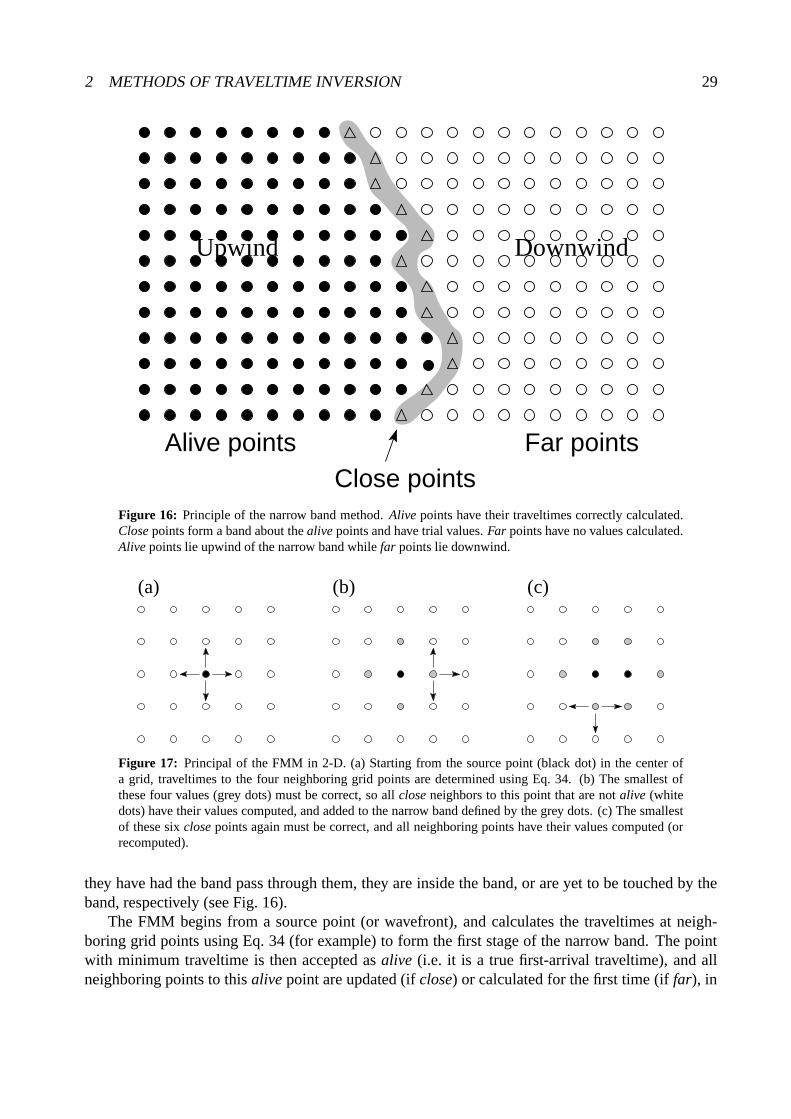
2 METHODS OF TRAVELTIME INVERSION 29
Upwind
Far pointsAlive pointsClose points
Downwind
Figure 16: Principle of the narrow band method. Alive points have their traveltimes correctly calculated.Close points form a band about the alive points and have trial values. Far points have no values calculated.Alive points lie upwind of the narrow band while far points lie downwind.
(a) (b) (c)
Figure 17: Principal of the FMM in 2-D. (a) Starting from the source point (black dot) in the center ofa grid, traveltimes to the four neighboring grid points are determined using Eq. 34. (b) The smallest ofthese four values (grey dots) must be correct, so all close neighbors to this point that are not alive (whitedots) have their values computed, and added to the narrow band defined by the grey dots. (c) The smallestof these six close points again must be correct, and all neighboring points have their values computed (orrecomputed).
they have had the band pass through them, they are inside the band, or are yet to be touched by theband, respectively (see Fig. 16).
The FMM begins from a source point (or wavefront), and calculates the traveltimes at neigh-boring grid points using Eq. 34 (for example) to form the first stage of the narrow band. The pointwith minimum traveltime is then accepted as alive (i.e. it is a true first-arrival traveltime), and allneighboring points to this alive point are updated (if close) or calculated for the first time (if far), in

2 METHODS OF TRAVELTIME INVERSION 30
which case they become close and the narrow band progresses downwind (see Fig. 17). Choosingthe close point with minimum traveltime means that causality is satisfied. The key to an efficient im-plementation of the narrow band scheme is to be able to rapidly locate the close point with minimumtraveltime. Heap sorting of traveltimes using a binary tree (Sethian & Popovici, 1999) means that theFMM will have an efficiency of O(N log N ) where N is the number of grid points. Fig. 18 shows awavefront calculated using the FMM propagating through a complex 2-D velocity model. Source-receiver ray paths, calculated by following the steepest descent direction (using Eq. 33) through thecomputed traveltime field from each receiver, are also shown. The velocity variations have beenmade extremely large to illustrate the robustness of the scheme, which remains stable despite thepropagating wavefront exhibiting significant discontinuities in gradient.
Figure 18: Example of the FMM in a complex 2-D velocity medium. The grid on which the eikonalequation is solved has a spacing of 200 m in both x and z; the total number of points is 100,701. Wavefrontsare shown by thin grey lines and are visualized at 0.5 s intervals; rays are denoted by black lines and arealways perpendicular to the wavefronts.
To increase the accuracy of the FMM scheme without increasing the number of grid points,higher order differences may be used to approximate the traveltime gradient (Popovici & Sethian,2002). However, since causality must be respected, they cannot simply replace the first-order dif-ferences in all cases (Sethian, 1999). Kim (2001) advocates using the average normal slowness si j k
in place of si j k to increase accuracy since velocities specified at grid points don’t account for thetrue variation across a cell. For point sources, Alkhalifah & Fomel (2001) suggest using a sphericalrather than Cartesian grid since the latter tends to under-sample the wavefront near the source wherecurvature is high, and hence introduces traveltime errors. This source of error occurs for any Carte-
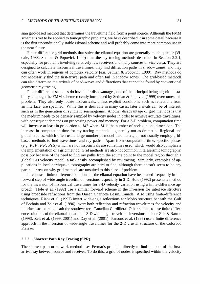
2 METHODS OF TRAVELTIME INVERSION 31
sian grid-based method that determines the traveltime field from a point source. Although the FMMscheme is yet to be applied to tomographic problems, we have described it in some detail because itis the first unconditionally stable eikonal scheme and will probably come into more common use inthe near future.
Finite difference grid methods that solve the eikonal equation are generally much quicker (Vi-dale, 1988; Sethian & Popovici, 1999) than the ray tracing methods described in Section 2.2.1,especially for problems involving relatively few receivers and many sources or vice versa. They aredesigned to calculate first-arrival traveltimes, they find diffraction paths in shadow zones, and theycan often work in regions of complex velocity (e.g. Sethian & Popovici, 1999). Ray methods donot necessarily find the first-arrival path and often fail in shadow zones. The grid-based methodscan also determine the arrivals of head-waves and diffractions that cannot be found by conventionalgeometric ray tracing.
Finite-difference schemes do have their disadvantages, one of the principal being algorithm sta-bility, although the FMM scheme recently introduced by Sethian & Popovici (1999) overcomes thisproblem. They also only locate first-arrivals, unless explicit conditions, such as reflections froman interface, are specified. While this is desirable in many cases, later arrivals can be of interest,such as in the generation of synthetic seismograms. Another disadvantage of grid methods is thatthe medium needs to be densely sampled by velocity nodes in order to achieve accurate traveltimes,with consequent demands on processing power and memory. For a 3-D problem, computation timewill increase at least in proportion to M3 where M is the number of nodes in one dimension. Theincrease in computation time for ray-tracing methods is generally not as dramatic. Regional andglobal studies, which often use a large number of model parameters, do not usually employ grid-based methods to find traveltimes and ray paths. Apart from computation time, specific phases(e.g. PcP , P P , PcS) which are not first-arrivals are sometimes used, which would also complicatethe implementation of a grid method. Grid methods are also not common in teleseismic tomography,possibly because of the need to find ray paths from the source point to the model region through aglobal 1-D velocity model, a task easily accomplished by ray tracing. Similarly, examples of ap-plications in local earthquake tomography are hard to find, although there doesn’t seem to be anyparticular reason why grid methods are unsuited to this class of problem.
In contrast, finite difference solutions of the eikonal equation have been used frequently in theforward step of wide-angle traveltime inversions, especially in 3-D. Hole (1992) presents a methodfor the inversion of first-arrival traveltimes for 3-D velocity variation using a finite-difference ap-proach. Hole et al. (1992) use a similar forward scheme in the inversion for interface structureusing broadside refractions from the Queen Charlotte Basin, Canada. Also using finite-differencetechniques, Riahi et al. (1997) invert wide-angle reflections for Moho structure beneath the Gulfof Bothnia and Zelt et al. (1996) invert both reflection and refraction traveltimes for velocity andinterface structure beneath the southwestern Canadian Cordillera. Other studies to use finite differ-ence solutions of the eikonal equation in 3-D wide-angle traveltime inversions include Zelt & Barton(1998), Zelt et al. (1999, 2001) and Day et al. (2001). Parsons et al. (1996) use a finite differenceapproach in the inversion of wide-angle traveltimes for the 2-D crustal structure of the ColoradoPlateau.
2.2.3 Shortest Path Ray Tracing (SPR)
The shortest path or network method uses Fermat’s principle directly to find the path of the first-arrival ray between source and receiver. To do this, a grid of nodes is specified within the velocity
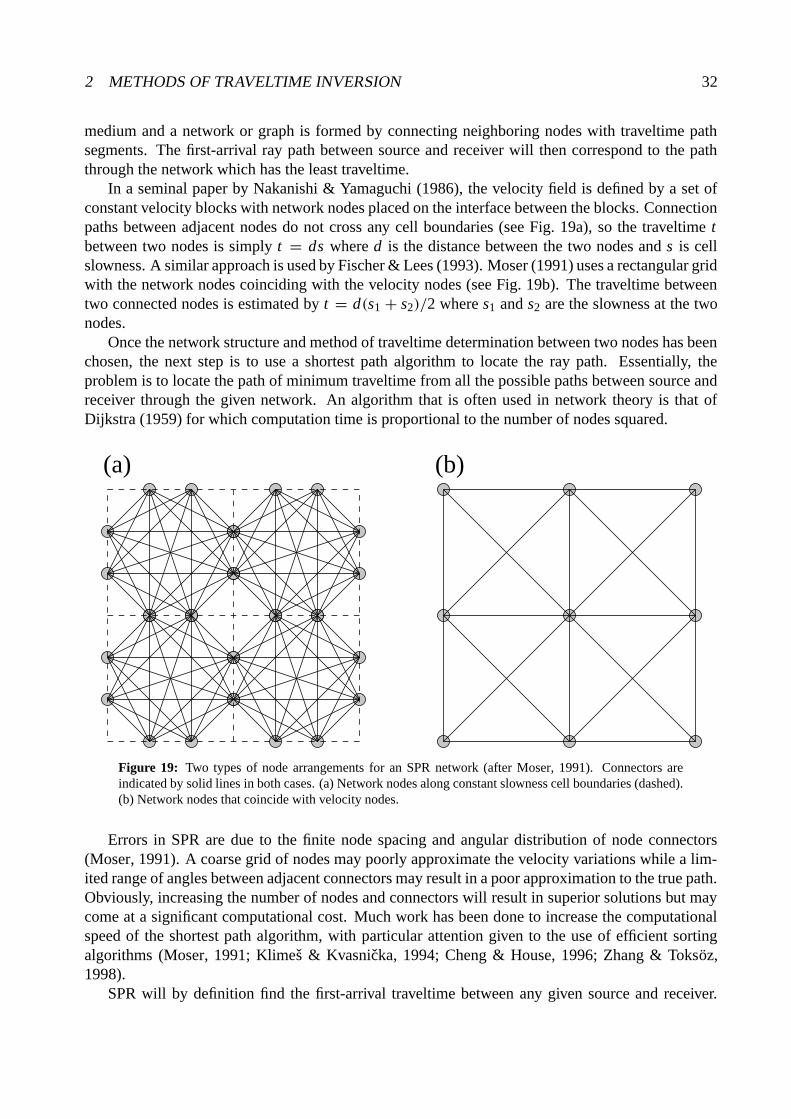
2 METHODS OF TRAVELTIME INVERSION 32
medium and a network or graph is formed by connecting neighboring nodes with traveltime pathsegments. The first-arrival ray path between source and receiver will then correspond to the paththrough the network which has the least traveltime.
In a seminal paper by Nakanishi & Yamaguchi (1986), the velocity field is defined by a set ofconstant velocity blocks with network nodes placed on the interface between the blocks. Connectionpaths between adjacent nodes do not cross any cell boundaries (see Fig. 19a), so the traveltime tbetween two nodes is simply t = ds where d is the distance between the two nodes and s is cellslowness. A similar approach is used by Fischer & Lees (1993). Moser (1991) uses a rectangular gridwith the network nodes coinciding with the velocity nodes (see Fig. 19b). The traveltime betweentwo connected nodes is estimated by t = d(s1 + s2)/2 where s1 and s2 are the slowness at the twonodes.
Once the network structure and method of traveltime determination between two nodes has beenchosen, the next step is to use a shortest path algorithm to locate the ray path. Essentially, theproblem is to locate the path of minimum traveltime from all the possible paths between source andreceiver through the given network. An algorithm that is often used in network theory is that ofDijkstra (1959) for which computation time is proportional to the number of nodes squared.
(a) (b)
Figure 19: Two types of node arrangements for an SPR network (after Moser, 1991). Connectors areindicated by solid lines in both cases. (a) Network nodes along constant slowness cell boundaries (dashed).(b) Network nodes that coincide with velocity nodes.
Errors in SPR are due to the finite node spacing and angular distribution of node connectors(Moser, 1991). A coarse grid of nodes may poorly approximate the velocity variations while a lim-ited range of angles between adjacent connectors may result in a poor approximation to the true path.Obviously, increasing the number of nodes and connectors will result in superior solutions but maycome at a significant computational cost. Much work has been done to increase the computationalspeed of the shortest path algorithm, with particular attention given to the use of efficient sortingalgorithms (Moser, 1991; Klimes & Kvasnicka, 1994; Cheng & House, 1996; Zhang & Toksoz,1998).
SPR will by definition find the first-arrival traveltime between any given source and receiver.
2 METHODS OF TRAVELTIME INVERSION 33
However, it is possible to impose constraints on the path so that some other arrivals such as reflectionsor multiples can be determined. Moser (1991) demonstrated a method for reflections which requiresthe shortest path to visit a specified set of nodes that lie on the interface.
In their original implementation of SPR, Nakanishi & Yamaguchi (1986) inverted traveltimesfrom local earthquakes, while Zhang & Toksoz (1998) used it in the inversion of refraction trav-eltimes. Toomey et al. (1994) inverted first-arrival refraction traveltimes for 3-D crustal velocitystructure using a scheme similar to that of Moser (1991) to solve the forward problem. Apart fromthese examples, the use of SPR in tomographic inversions is not common. SPR shows similar ad-vantages to finite differences (see Section 2.2.2) relative to conventional ray tracing methods. It cancorrectly locate diffraction paths and head waves and always finds first-arrivals. The main advantageSPR has over most finite difference methods is robustness; it is capable of working in highly com-plex media. Cheng & House (1996) claim it to be the most robust numerical scheme for traveltimecalculations, although the introduction of the FMM challenges this claim. SPR methods also tend tobe slower than eikonal methods.
2.3 Solving the Inverse Step
The inversion step, which involves the adjustment of the model parameters m to better satisfy theobserved data dobs through the known relationship d = g(m), can be performed in a number of ways.In traveltime tomography, the functional g is non-linear because the ray path depends on the velocitystructure. Ideally, an inversion scheme should account for this non-linearity. The three approachesto solving the inversion step that will be considered below are backprojection, gradient methods andglobal optimization techniques.
2.3.1 Backprojection
In Section 1.2, we showed that the perturbation of a ray path only has a second order effect ontraveltime. In terms of slowness, this was written (see Eq. 7):
δt =∫
L0
δs(x)dl + O(δs(x)2) (37)
If a continuum is described by M constant slowness blocks, then the discrete form of Eq. 37 for Nrays can be written:
d = Gm (38)
where d are the traveltime residuals, m the slowness perturbations and G an N × M matrix of raylengths li j corresponding to the distance traversed by each ray in each block. Note that for the generalcase m (e.g. velocity nodes, interface depths etc.) in Eq. 38, G = ∂g/∂m where g(m) is the modelprediction. Many of the elements of G will be zero since each ray path will usually only traverse asmall subset of the M blocks. Backprojection methods can be used to solve Eq. 38 for the slownessperturbations m by iteratively mapping traveltime anomalies into slowness perturbations along theray paths until the data are satisfied. Backprojection methods generally use constant slowness (orvelocity) blocks. Two well known backprojection techniques for solving Eq. 38 are the AlgebraicReconstruction Technique (ART) and the Simultaneous Iterative Reconstruction Technique (SIRT),both of which originate from medical imaging.

2 METHODS OF TRAVELTIME INVERSION 34
In ART, the model is updated on a ray by ray basis. The residual dn for the nth ray path isdistributed along the path by adjusting each component of m in proportion to the length lnj of theray segment in the j th cell:
mk+1j = mk
j + tk+1n lnj
M∑
m=1l2nm
(39)
where tk+1n = dn − tk
n is the difference between the residuals at the 0th and kth iteration, mkj is the
approximation to the j th model parameter at the k th iteration, m1j = 0 and t1
n = 0. The residual
along the (n + 1)th ray is then determined for the updated velocity field m using the original pathand is backprojected in the same manner. A single iteration of the method consists of performing thisbackprojection for the N ray paths. Rays are then retraced and the backprojection repeated until thedata are satisfied to within tolerance, or the solution converges. The main problem with ART is thatit suffers from poor convergence properties (Blundell, 1993). It has been used by McMechan (1983)in cross-hole tomography and Nakanishi & Yamaguchi (1986) in local earthquake tomography.
SIRT addresses some of the convergence problems associated with ART by averaging the pertur-bations applied to each parameter from all the rays that are influenced by the parameter. Thus, theSIRT algorithm may be written (Blundell, 1993):
mk+1j = mk
j + 1
Rkj
Rkj
∑
n=1
tk+1n lnj
M∑
m=1l2nm
(40)
where Rkj is the number of rays that the j th model parameter influences for the k th iteration. The
SIRT method has been used in the inversion of teleseismic traveltime residuals by Dueker et al.(1993), Granet & Trampert (1989) and McQueen & Lambeck (1996). Blundell (1993) used SIRT(as well as other methods) in the inversion of reflection traveltimes for both velocity structure andinterface depth.
Authors who have used variants of these backprojection schemes include Humphreys & Clayton(1990), Hole (1992) and Zelt & Barton (1998). Humphreys & Clayton (1990) used block subbinning,filtering and spatial averaging in the backprojected inversion of teleseismic traveltimes. Block sub-binning reduces the weight of rays that come from dominant directions, and thus reduces blurring ofthe image along these paths. Filtering is done using point spread functions to reduce the natural ten-dency of backprojection to blur an image if resolution is not perfect, and spatial averaging is used tosmooth the solution. Hole (1992) also uses smoothing in the backprojected inversion of wide-angletraveltimes. Zelt & Barton (1998), in their 3-D wide-angle seismic inversion method, implementseveral other modifications aimed at improving the convergence and accuracy of backprojection.
Inversion using backprojection tends to be computationally more rapid at each iteration com-pared to other techniques, but often converges more slowly and with less stability. This is at leastpartly due to the use of more ad hoc regularization (like spatial averaging) compared to, for example,the formal inclusion of such constraints in the inversion permitted by gradient methods.
2 METHODS OF TRAVELTIME INVERSION 35
2.3.2 Gradient Methods
The inverse problem in seismic tomography can be formulated as one of minimizing an objectivefunction consisting of a data residual term and one or more regularization terms. As before, let d de-note a data vector of length N which is dependent on a model vector m of length M as d = g(m). Foran initial estimate m0 of the model parameters, comparing d = g(m0) with the observed traveltimesdobs gives an indication of the accuracy of the model. The misfit can be quantified by constructingan objective function S(m), consisting of a weighted sum of data misfit and regularization terms,that is to be minimized.
An essential component of the objective function is a term 9(m) which measures the differencebetween the observed and predicted data. If it is assumed that the error in the relationship dobs ≈g(mtrue) is Gaussian, then a least squares or L2 measure of this difference is suitable:
9(m) = ‖g(m)− dobs‖2 (41)
If uncertainty estimates have been made for the observed data (usually based on picking error), thenmore accurate data are given a greater weight in the objective function by writing 9(m) as:
9(m) = (g(m)− dobs)T C−1
d (g(m)− dobs) (42)
where Cd is a data covariance matrix. If the errors are assumed to be uncorrelated, then Cd =[δi j (σ
jd )
2] where σ jd is the uncertainty of the j th traveltime. Strictly speaking, Cd is best referred to
as a data weighting matrix rather than a data covariance matrix unless it truly reflects the uncertaintyassociated with the data. A major weakness in this definition of data misfit is that the L2-norm issensitive to outliers. This means that if only a few data have spurious values (e.g. from incorrectphase identification), then they will have a significant influence on the size of 9(m) since eachresidual is squared; the L2-norm is a non-robust measure. A solution produced by the minimizationof9(m) is then likely to be less reliable than one produced using, for example, an L 1 norm (Menke,1989). Despite this weakness, most inversion methods appeal to Gaussian statistics and adopt an L 2
norm. See Claerbout & Muir (1973) for a discussion of robustness in error distribution.A common problem with tomographic inversion is that not all model parameters will be well
constrained by the data alone (i.e. the problem may be under-determined or mixed-determined). Aregularization term8(m) is often included in the objective function to provide additional constraintson the model parameters, thereby reducing the non-uniqueness of the solution. The regularizationterm is typically defined as:
8(m) = (m − m0)T C−1
m (m − m0) (43)
where Cm is an a priori model covariance matrix. If uncertainties in the initial model are assumedto be uncorrelated, then Cm = [δi j (σ
jm)
2] where σ jm is the uncertainty associated with the j th model
parameter of the initial model. Again, this should really be referred to as a model weighting matrixunless its entries reflect the true statistical uncertainties of the initial model. The effect of8(m) is toencourage solution models m that are near a reference model m0. The values used in Cm are usuallybased on prior information.
Another approach to regularization is the minimum structure solution (Constable et al., 1987)which attempts to find an acceptable trade-off between satisfying the data and finding a model withthe minimum amount of structural variation. One way of including this requirement in the objectivefunction is to use the term (Sambridge, 1990):
�(m) = mT DT Dm (44)

2 METHODS OF TRAVELTIME INVERSION 36
where Dm is a finite difference estimate of a specified spatial derivative. For example, ifm1,m2, . . . ,m M represent contiguous depth nodes of an interface in 2-D space, then the gradient ofthe interface could be regulated using:
Dm =
−1 1 0 . . . . . . 00 −1 1 0 . . . 0. . . 0 . . . . . . . . . . . .
. . . . . . . . . . . . . . . . . .
. . . . . . . . . 0 −1 1
. . . . . . . . . . . . 0 0
m1
m2
m3
. . .
mM−1
mM
(45)
Alternatively, the curvature of the interface could be regulated using:
Dm =
0 0 0 0 . . . 01 −2 1 0 . . . 00 1 −2 1 . . . . . .
. . . . . . . . . . . . . . . . . .
. . . . . . . . . 1 −2 1
. . . . . . . . . . . . 0 0
m1
m2
m3
. . .
mM−1
mM
(46)
An explicit smoothing term such as Eq. 46 in the objective function may be necessary if crude pa-rameterizations such as constant velocity blocks are used to simulate a continuously varying velocityfield. However, if an implicitly smooth parameterization like cubic splines is used, then an explicitsmoothing term may be unnecessary. In other words, the same smooth result could be achieved byreducing the number of parameters and hence the size of the inverse problem. The appropriate num-ber of parameters required to represent the model for a given dataset could be chosen on a statisticalbasis, such as employing the F test (Menke, 1989).
Using the L2 terms described above in Equations 42 - 44, the objective function S(m) can bewritten in full as:
S(m) = 1
2[9(m)+ ε8(m)+ η�(m)] (47)
where ε is referred to as the damping factor and η as the smoothing factor (when D is the secondderivative operator, which is usually the case). Multiplication of all terms by 1/2 is done simply toprevent the expressions for the first and second derivatives of S having all elements multiplied by2 (see Eq. 49 and Eq. 50). ε and η govern the trade-off between how well the solution mest willsatisfy the data, how closely mest is to m0, and the smoothness of mest . There are several meansfor choosing appropriate values for ε and η. One way is to use the largest values of ε and η forwhich the data are still satisfied, but there will be a trade-off between ε and η. When only dampingor smoothing is invoked, then this approach is simpler to implement. However, it may be that therelationship between the data fit and the model perturbation or model roughness is highly non-linear,in which case this criterion may not be robust. A better approach is to inspect the trade-off curvesbetween data fit and model roughness (or perturbation) for different values of η (or ε), as shownschematically in Fig. 20. If both η and ε are non-zero, then a contour plot which shows traveltimefit contoured on a plot of model roughness vs. model perturbation (Fig. 21) could be used, but themain drawback here is the considerable computational effort required. An alternative approach is toperform a synthetic reconstruction using the same source-receiver geometry as the real experiment.The appropriate amount of damping and smoothing would then be given by the values of η and εwhich resulted in the most accurate reconstruction of the synthetic model.
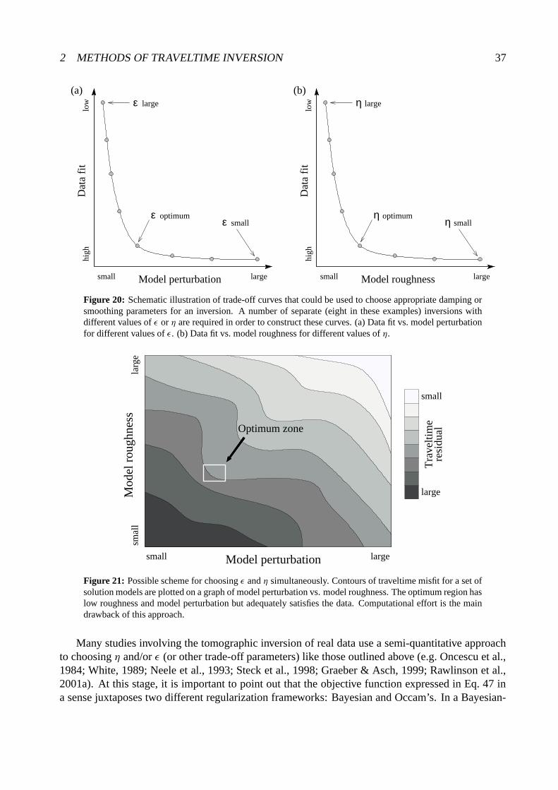
2 METHODS OF TRAVELTIME INVERSION 37
Model perturbation
ηη
η(b)
smalloptimum
large
small large
low
high
Dat
a fi
t
Model roughness
(a)
small
Dat
a fi
thi
ghlo
w
largesmall
ε
εε
large
optimum
Figure 20: Schematic illustration of trade-off curves that could be used to choose appropriate damping orsmoothing parameters for an inversion. A number of separate (eight in these examples) inversions withdifferent values of ε or η are required in order to construct these curves. (a) Data fit vs. model perturbationfor different values of ε. (b) Data fit vs. model roughness for different values of η.
Tra
velti
me
resi
dual
large
small
larg
esm
all
Model perturbationsmall large
Mod
el r
ough
ness
Optimum zone
Figure 21: Possible scheme for choosing ε and η simultaneously. Contours of traveltime misfit for a set ofsolution models are plotted on a graph of model perturbation vs. model roughness. The optimum region haslow roughness and model perturbation but adequately satisfies the data. Computational effort is the maindrawback of this approach.
Many studies involving the tomographic inversion of real data use a semi-quantitative approachto choosing η and/or ε (or other trade-off parameters) like those outlined above (e.g. Oncescu et al.,1984; White, 1989; Neele et al., 1993; Steck et al., 1998; Graeber & Asch, 1999; Rawlinson et al.,2001a). At this stage, it is important to point out that the objective function expressed in Eq. 47 ina sense juxtaposes two different regularization frameworks: Bayesian and Occam’s. In a Bayesian-
2 METHODS OF TRAVELTIME INVERSION 38
style inversion, knowledge of a priori information is of paramount importance. To properly honorthis approach, smoothing would be ignored (i.e. set η=0), the data covariance matrix would reflectthe known statistical properties of the data and the initial model estimate would be based on apriori model information. In addition, we would set ε = 1 since the a priori model covariancematrix would reflect the uncertainties associated with the a priori information. Minimization of theobjective function then results in a solution that assimilates the information contained in the datawith the a priori information, resulting in an a posteriori model distribution. The posterior modeluncertainties should then be less than the prior uncertainties, which is the desired outcome (howmuch less depends on how good the data are). The principal difficulty with this approach is thatmeaningful a priori information concerning model and data errors is difficult to obtain in practice.Nevertheless, this Bayesian approach has been adopted by a number of authors (e.g. Aki et al., 1977;Lutter & Nowack, 1990). Scales & Snieder (1997) discuss the merits and difficulties of adopting aBayesian framework for inversion.
The other regularization framework is suggested by Occam’s principle of seeking a solution withthe least structure necessary to fit the data (Constable et al., 1987). In this case ε = 0 since we don’twant the initial model, whose accuracy is poorly known, to unduly influence the solution model. Thistype of scheme is also popular (e.g. Sambridge, 1990; Zelt & Barton, 1998; Day et al., 2001). Often,however, a mixture of both frameworks is used, in which case one seeks a physically reasonablemodel that contains no unnecessary structure, is not highly perturbed from the initial model andsatisfies the data. This explains to some extent why the choice of ε and η is often subjective.
Gradient-based inversion methods make use of the derivatives of S(m) at a specified point inmodel space. A basic assumption that is shared by all practical gradient methods is that S(m) issufficiently smooth to allow a local quadratic approximation about some current model:
S(m + δm) ≈ S(m)+ γγγ δm + 12δm
T Hδm (48)
where δm is a perturbation to the current model and γγγ = ∂S/∂m and H = ∂2S/∂m2 are the gradientvector and Hessian matrix respectively. Evaluating these partial derivatives for Eq. 47 gives:
γγγ = GT C−1d [g(m)− dobs] + εC−1
m (m − m0)+ ηDT Dm (49)
H = GT C−1d G + ∇mGT C−1
d [g(m)− dobs] + εC−1m + ηDT D (50)
where G = ∂g/∂m is the Frechet matrix of partial derivatives calculated during the solution of theforward problem. As mentioned earlier, for the case of constant slowness blocks, G = [li j ] whereli j is the ray segment length of the i th ray in the j th block. Usually, the second derivative term inH is neglected since it is time consuming to evaluate, and its effect is small if g(m)− dobs is small,or if the forward problem is quasi-linear (∇mG ≈ 0). Both γγγ and H do not lie in model space, butin the dual of model space (Tarantola, 1987). If γγγ is the steepest ascent vector in model space thenγγγ = Cm γγγ and H, the curvature operator in model space, is H = CmH.
Since g is generally non-linear, the minimization of Eq. 47 requires an iterative approach:
mn+1 = mn + δmn (51)
where m0 is the initial model. The objective function is minimized for the current ray path estimateat each step to produce mn+1, after which new ray paths are computed for the next iteration. Theiterations cease either when the observed traveltimes are satisfied or when the change in S(m) with

2 METHODS OF TRAVELTIME INVERSION 39
iteration gets sufficiently small. A useful measure of data fit is provided by the normalized χ 2 misfitfunction defined by:
χ2 = 1
N
N∑
i=1
(
d im − d i
obs
σ id
)2
(52)
where {d im} = g(m), {d i
obs} is the set of observed data and {σ id} are the traveltime uncertainties
(or weights). An inversion solution fits the data to the level of the noise when χ 2 = 1. Once thisvalue is achieved, there is little point in continuing with the iterative inversion process. However,Eq. 52 measures the data fit in an average sense, and it is still possible to have χ 2 < 1 while oneor more model traveltime residuals are larger than their respective error estimates. If the data misfitdoes not fall below χ2 = 1, then statistical hypothesis testing (e.g. Kreyszig, 1993) can be usedto stop the iterative process. For example, if the data misfit has a normal distribution, we can testwhether the data variance at iteration n is significantly different from the variance at iteration n + 1(usually referred to as an F -test). The F -test has been used by numerous authors (e.g. Thurber,1983; Eberhart-Phillips, 1986; Steck et al., 1998; Graeber & Asch, 1999).
The following gradient-based inversion methods can be used to determine δmn in Eq. 51.
2.3.2.1 Gauss-Newton method and damped-least squares The Gauss-Newton method locatesthe updated point mn+1 by finding the minimum of the tangent paraboloid to S(m) at mn . At theminimum of S, the gradient will vanish, so m is required such that:
F(m) = GT C−1d (g(m)− dobs)+ εC−1
m (m − m0)+ ηDT Dm = 0 (53)
where F(m) = γγγ . If we are at some point mn , then a more accurate estimate mn+1 can be obtainedusing a Taylor series expansion of Eq. 53 and ignoring second order terms:
Fi (m1n+1, . . . ,m M
n+1) = Fi(m1n, . . . ,m M
n )+M∑
j=1
(m jn+1 − m j
n)∂Fi
∂m j
∣
∣
∣
∣
mn
= 0 (54)
which may be rewritten as:
mn+1 = mn −[
∂F∂m
]−1
n[Fn] = mn −
[
∂2S
∂m2
]−1
n
[
∂S
∂m
]
n(55)
where (∂S/∂m)n is the gradient vector and (∂2S/∂m2)n is the Hessian matrix. Substituting Eq. 49and Eq. 50 into Eq. 55 gives the Gauss-Newton solution:
δmn = −[GTn C−1
d Gn + ∇mGTn C−1
d (g(mn)− dobs)+ εC−1m + ηDT D]−1
×[GTn C−1
d [g(mn)− dobs] + εC−1m (mn − m0)+ ηDT Dmn] (56)
As mentioned earlier, the second derivative term in the Hessian matrix is usually ignored, whichgives the quasi-Newton solution:
δmn = −[GTn C−1
d Gn + εC−1m + ηDT D]−1[GT
n C−1d [g(mn)− dobs]
+εC−1m (mn − m0)+ ηDT Dmn] (57)

2 METHODS OF TRAVELTIME INVERSION 40
Straightforward implementation of this method requires an M × M matrix equation to be solved. Ifthe number of model parameters is large, the solution will be computationally expensive, and if datacoverage is poor, the problem may well be ill-conditioned.
If instead we assume that the relationship d = g(m) is linearizable then (c.f. Eq. 38):
dobs ≈ g(m0)+ G(m − m0) (58)
or δd = Gδm with δd = dobs − g(m0) and δm = m − m0 (i.e. Eq. 38 with G = ∂g/∂m). If Eq. 58is exactly linear, then the Newton and quasi-Newton solutions are the same because the secondderivative terms in the Hessian matrix are zero. Because a one-step solution is possible in the linearcase, the objective function is sometimes written:
S(m) = 1
2
[
(Gδm − δd)T C−1d (Gδm − δd)+ εδmT C−1
m δm + ηδmT DT Dδm]
(59)
where last term on the RHS smooths the perturbations to the prior model. The functional in this caseis:
F(m) = GT C−1d (Gδm − δd)+ εC−1
m δm + ηDT Dδm = 0 (60)
and the solution can be written as:
δm = [GT C−1d G + εC−1
m + ηDT D]−1GT C−1d δd (61)
When no smoothing is used (η = 0) and the matrices Cd and Cm represent the known a priori errorstatistics, then Eq. 61 becomes:
δm = [GT C−1d G + C−1
m ]−1GT C−1d δd (62)
which is the maximum likelihood solution to the inverse problem or the stochastic inverse (Aki et al.,1977). The expressions for δm in Eq. 57, Eq. 61 or Eq. 62 are often referred to as Damped LeastSquares (DLS) solutions to the inverse problem (particularly when η = 0).
It is interesting to note the differences between the solution given by Eq. 57 and Eq. 61. First,the smoothing term in Eq. 61 smoothes the perturbations to the model, not the model itself. Second,if Eq. 61 is applied iteratively, then the damping regularization is not necessarily the same as thatimposed by the iterative implementation of Eq. 57. In the latter, the term m0 usually represents theinitial or starting model and the effect of the regularization is to favor a solution near the initial model(how “near” will depend on the value of ε). If, however, m0 = mprior , where mprior is the solutionat the previous iteration, then the damping in Eq. 57 will be the same as that for Eq. 61, in whichthe misfit of the current model compared to the previous model is regulated. In damping, the use ofm0 is often referred to as “jumping” while using mprior is often referred to as “creeping” (Shaw &Orcutt, 1985). Similarly, smoothing the perturbation to the model is “creeping” while smoothing themodel is “jumping”. The DLS-type solution scheme is the technique most commonly used to solvethe inverse step in seismic tomography. Many other variants to those discussed above have also beenused - Spakman (1993) describes and compares several of them.
Studies that have used a DLS-type solution to the inverse problem in teleseismic tomographyinclude those by Aki et al. (1977), Zhao et al. (1994), Weiland et al. (1995), Wiggins et al. (1996) andSteck et al. (1998). Authors who have used DLS solutions to invert wide-angle traveltimes includeKanasewich & Chiu (1985), Chiu et al. (1986), Farra & Madariaga (1988), White (1989), Lutter &
2 METHODS OF TRAVELTIME INVERSION 41
Nowack (1990), Lutter et al. (1990), Zelt & Smith (1992), Lutter et al. (1994), Kosloff et al. (1996),Wang & Braile (1996), McCaughey & Singh (1997) and Zelt & Barton (1998). Similarly, DLS isalso popular in local earthquake tomography (Aki & Lee, 1976; Thurber, 1983; Eberhart-Phillips,1986; Zhao et al., 1992; Graeber & Asch, 1999).
The most computationally expensive part of the DLS solution is to solve a matrix equation ofdimension M . If the number of parameters is not large, then the solution may be found using meth-ods like LU decomposition (Press et al., 1992) or Cholesky decomposition (Tarantola, 1987). Aparticularly useful solution technique for small to mid-size problems is Singular Value Decomposi-tion (Press et al., 1992) or SVD. It is capable of robustly dealing with matrices that are singular ornearly singular, which is often the case in tomographic problems. In addition, SVD can be used todiagnose problems with the system of equations, such as the presence of equations that do not helpconstrain the solution. Another attractive feature of SVD is that covariance and resolution estimatesassociated with the solution model may be obtained at virtually no extra cost (e.g. White, 1989).
For models defined by large numbers of parameters, direct solution methods are cumbersomeand iterative techniques are more practical. One such method is the conjugate gradient method ofHestenes & Stiefel (1952), which is able to take advantage of the sparse nature of linear systemscommonly associated with seismic tomography problems (Scales, 1987). Conjugate gradients andLSQR, a variant of the conjugate gradient algorithm, are probably the most commonly used methodsfor solving linear systems of the form of Eq. 61 with a large number (e.g. 1000’s - 100,000’s) ofunknowns (Nolet, 1985; Scales, 1987; VanDecar & Snieder, 1994).
The DLS-type solution to the inverse problem need not be formulated as a set of normal equa-tions, such as Eq. 57 or Eq. 62. For example, Eq. 59 may be minimized by finding the least squaressolution of the system:
C−1/2d G√εC−1/2
m√ηD
δm =
C−1/2d δd
00
(63)
which is equivalent to solving Eq. 61. SVD or iterative solvers like LSQR can be used to solveEq. 63 since they can equally well be applied to non-square systems and will solve the equations inthe least-squares sense.
2.3.2.2 Steepest descent The method of steepest descent is probably the simplest gradient-basedmethod for iterative minimization of an objective function. It is based on the idea that the objectivefunction S may be minimized by successive searches along local directions of steepest descent. Ifγγγ n is the direction of steepest ascent in model space at a point mn, the model correction is given by:
δmn = −µnγγγ n (64)
where the scalar µn is a positive real number whose value locates the minimum in the directionspecified by γγγ n. The parameter µn can be found by line minimization as follows. By assumingthat g(m) is locally linear, so that g(mn+1) = g(mn)+ Gn(mn+1 − mn), then S(m) is quadratic so∂S(m)/∂µn = 0 will give the value of µn . Substituting Eq. 64 into Eq. 48 gives:
S(mn − µnγγγ n) = S(mn)− µn γγγTn γγγ n + 1
2µ2nγγγ
Tn Hnγγγ n (65)
The partial derivative of Eq. 65 is:
∂S(mn − µnγγγ n)
∂µn= −γγγ T
n γγγ n + µnγγγTn Hnγγγ n = 0 (66)
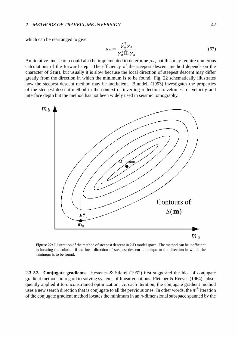
2 METHODS OF TRAVELTIME INVERSION 42
which can be rearranged to give:
µn = γγγTn γγγ n
γγγ Tn Hnγγγ n
(67)
An iterative line search could also be implemented to determine µn , but this may require numerouscalculations of the forward step. The efficiency of the steepest descent method depends on thecharacter of S(m), but usually it is slow because the local direction of steepest descent may differgreatly from the direction in which the minimum is to be found. Fig. 22 schematically illustrateshow the steepest descent method may be inefficient. Blundell (1993) investigates the propertiesof the steepest descent method in the context of inverting reflection traveltimes for velocity andinterface depth but the method has not been widely used in seismic tomography.
γ0
Minimum
Contours ofS )m
m 0
m b
m a
(
Figure 22: Illustration of the method of steepest descent in 2-D model space. The method can be inefficientin locating the solution if the local direction of steepest descent is oblique to the direction in which theminimum is to be found.
2.3.2.3 Conjugate gradients Hestenes & Stiefel (1952) first suggested the idea of conjugategradient methods in regard to solving systems of linear equations. Fletcher & Reeves (1964) subse-quently applied it to unconstrained optimization. At each iteration, the conjugate gradient methoduses a new search direction that is conjugate to all the previous ones. In other words, the n th iterationof the conjugate gradient method locates the minimum in an n-dimensional subspace spanned by the
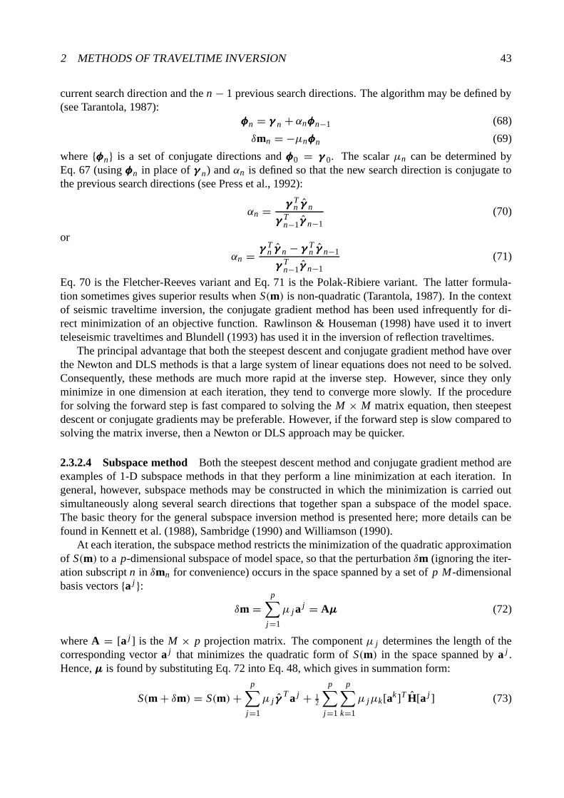
2 METHODS OF TRAVELTIME INVERSION 43
current search direction and the n − 1 previous search directions. The algorithm may be defined by(see Tarantola, 1987):
φφφn = γγγ n + αnφφφn−1 (68)
δmn = −µnφφφn (69)
where {φφφn} is a set of conjugate directions and φφφ0 = γγγ 0. The scalar µn can be determined byEq. 67 (using φφφn in place of γγγ n) and αn is defined so that the new search direction is conjugate tothe previous search directions (see Press et al., 1992):
αn = γγγ Tn γγγ n
γγγ Tn−1γγγ n−1
(70)
or
αn = γγγ Tn γγγ n − γγγ T
n γγγ n−1
γγγ Tn−1γγγ n−1
(71)
Eq. 70 is the Fletcher-Reeves variant and Eq. 71 is the Polak-Ribiere variant. The latter formula-tion sometimes gives superior results when S(m) is non-quadratic (Tarantola, 1987). In the contextof seismic traveltime inversion, the conjugate gradient method has been used infrequently for di-rect minimization of an objective function. Rawlinson & Houseman (1998) have used it to invertteleseismic traveltimes and Blundell (1993) has used it in the inversion of reflection traveltimes.
The principal advantage that both the steepest descent and conjugate gradient method have overthe Newton and DLS methods is that a large system of linear equations does not need to be solved.Consequently, these methods are much more rapid at the inverse step. However, since they onlyminimize in one dimension at each iteration, they tend to converge more slowly. If the procedurefor solving the forward step is fast compared to solving the M × M matrix equation, then steepestdescent or conjugate gradients may be preferable. However, if the forward step is slow compared tosolving the matrix inverse, then a Newton or DLS approach may be quicker.
2.3.2.4 Subspace method Both the steepest descent method and conjugate gradient method areexamples of 1-D subspace methods in that they perform a line minimization at each iteration. Ingeneral, however, subspace methods may be constructed in which the minimization is carried outsimultaneously along several search directions that together span a subspace of the model space.The basic theory for the general subspace inversion method is presented here; more details can befound in Kennett et al. (1988), Sambridge (1990) and Williamson (1990).
At each iteration, the subspace method restricts the minimization of the quadratic approximationof S(m) to a p-dimensional subspace of model space, so that the perturbation δm (ignoring the iter-ation subscript n in δmn for convenience) occurs in the space spanned by a set of p M-dimensionalbasis vectors {a j }:
δm =p∑
j=1
µ j a j = Aµµµ (72)
where A = [a j ] is the M × p projection matrix. The component µ j determines the length of thecorresponding vector a j that minimizes the quadratic form of S(m) in the space spanned by a j .Hence, µµµ is found by substituting Eq. 72 into Eq. 48, which gives in summation form:
S(m + δm) = S(m)+p∑
j=1
µ j γγγT a j + 1
2
p∑
j=1
p∑
k=1
µ jµk[ak]T H[a j ] (73)
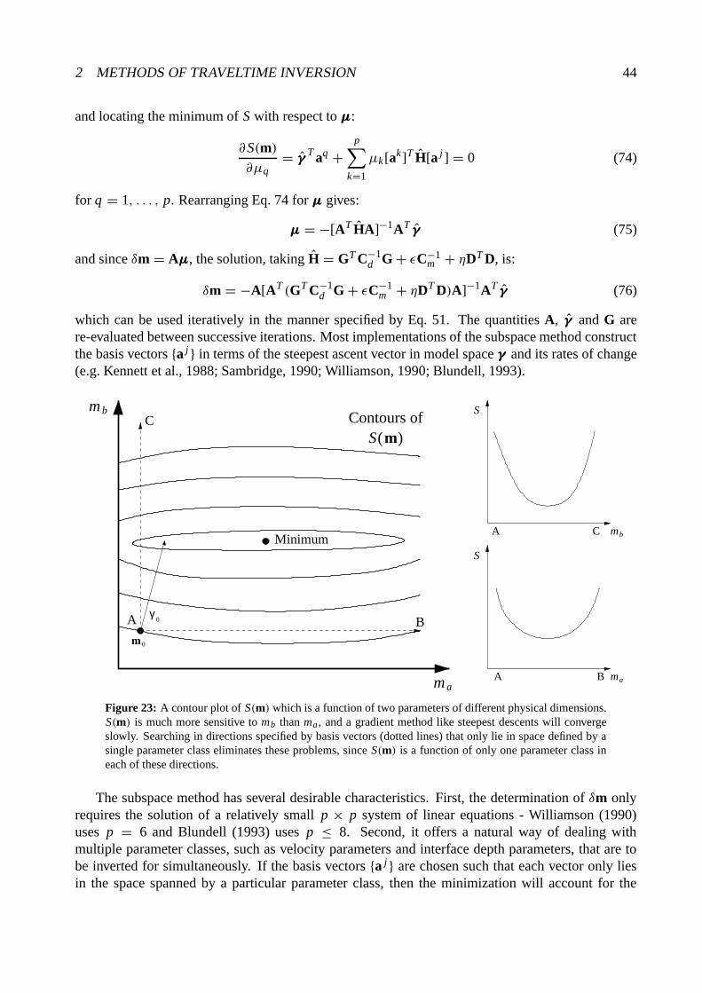
2 METHODS OF TRAVELTIME INVERSION 44
and locating the minimum of S with respect to µµµ:
∂S(m)∂µq
= γγγT aq +
p∑
k=1
µk[ak]T H[a j ] = 0 (74)
for q = 1, . . . , p. Rearranging Eq. 74 for µµµ gives:
µµµ = −[AT HA]−1AT γγγ (75)
and since δm = Aµµµ, the solution, taking H = GT C−1d G + εC−1
m + ηDT D, is:
δm = −A[AT (GT C−1d G + εC−1
m + ηDT D)A]−1AT γγγ (76)
which can be used iteratively in the manner specified by Eq. 51. The quantities A, γγγ and G arere-evaluated between successive iterations. Most implementations of the subspace method constructthe basis vectors {a j } in terms of the steepest ascent vector in model space γγγ and its rates of change(e.g. Kennett et al., 1988; Sambridge, 1990; Williamson, 1990; Blundell, 1993).
m 0
γ0
mb
ma
Minimum
S
S
A C
A Ba
Contours ofS )m
m b
m
(
A B
C
Figure 23: A contour plot of S(m) which is a function of two parameters of different physical dimensions.S(m) is much more sensitive to mb than ma , and a gradient method like steepest descents will convergeslowly. Searching in directions specified by basis vectors (dotted lines) that only lie in space defined by asingle parameter class eliminates these problems, since S(m) is a function of only one parameter class ineach of these directions.
The subspace method has several desirable characteristics. First, the determination of δm onlyrequires the solution of a relatively small p × p system of linear equations - Williamson (1990)uses p = 6 and Blundell (1993) uses p ≤ 8. Second, it offers a natural way of dealing withmultiple parameter classes, such as velocity parameters and interface depth parameters, that are tobe inverted for simultaneously. If the basis vectors {a j } are chosen such that each vector only liesin the space spanned by a particular parameter class, then the minimization will account for the

2 METHODS OF TRAVELTIME INVERSION 45
different sensitivities of S(m) with respect to the different parameter classes in a balanced way (seeFig. 23). Other gradient methods in which parameters of different physical dimensions are mixedcan exhibit slow convergence and a strong dependence on relative scaling of the different parametertypes (Kennett et al., 1988).
As an example of how one might choose a set of basis vectors, consider an inverse problem thathas three different parameter classes that are to be constrained by the data. Three separate searchdirections can simply be obtained by partitioning the gradient vector in model space γγγ = Cm γγγ onthe basis of parameter class:
γγγ = a1 + a2 + a3 =
γγγ 1
00
+
0γγγ 2
0
+
00γγγ 3
(77)
where a1, a2 and a3 represent ascent vectors that lie in the space of only one parameter type. A fur-ther nine basis vectors can be obtained by pre-multiplying a1, a2 and a3 by the model space HessianH = CmH and partitioning the three vectors that result in the same way as Eq. 77. Additional basisvectors can be produced by repeating the process of pre-multiplication of the latest set of vectorsby the partitioned model space Hessian. Once the required number of basis vectors is obtained,Gram-Schmidt orthogonalization should be applied to avoid interdependence:
aior th = ai −
i−1∑
j=1
ai · a j
a j · a ja j (78)
for i = 1, . . . , p. The basis vectors {aior th} are normalized and used in Eq. 76 via the projection
matrix A. If the subspace is large, then SVD may be more effective in finding the orthonormal set ofsubspace vectors due to the build-up of round-off error associated with the numerical implementationof Eq. 78 (Press et al., 1992). Choosing an appropriate number of basis vectors requires finding anacceptable balance between computational effort and rate of convergence.
Subspace methods have been applied to the inversion of reflection traveltimes for velocity andinterface structure (Williamson, 1990; Blundell, 1993), to the inversion of local earthquake andartificial source traveltimes for velocity, interface structure and hypocenter location (Sambridge,1990) and to the inversion of reflection amplitude data for interface structure (Wang & Houseman,1994) and velocity (Wang & Houseman, 1995). Rawlinson et al. (2001a,b) use it in the inversion ofrefraction and wide-angle reflection traveltimes for the determination of layered crustal structure.
2.3.2.5 Frechet matrix All gradient methods require the calculation of G = ∂g/∂m, which de-scribes the rate of change of traveltimes with respect to model parameters. For such discrete models,G defines the “Gateaux” derivative of g; the term “Frechet” derivative should really only be usedto describe the derivative of g for a continuous model (Shaw & Orcutt, 1985). However, since Gis widely referred to as the Frechet derivative/matrix even if the model is discrete, we will continueto do so here. The two basic parameter types that are normally encountered in traveltime inversion,especially of wide-angle data, are velocity (or slowness) and interface depth. First-order accurateexpressions for the derivatives can be derived quite simply for both cases. They are usually calcu-lated as part of the forward step of the tomographic problem. In local earthquake tomography, thesource location is also an unknown, so derivatives of traveltime with respect to these parameters arerequired.

2 METHODS OF TRAVELTIME INVERSION 46
The linearized relationship between traveltime residual and velocity perturbation was given byEq. 6:
δt = −∫
L(v0)
δv
v20
dl (79)
where δv is the velocity perturbation and v0 is the reference velocity field. If the velocity field isdefined by a grid of velocity nodes, then to first-order the Frechet derivatives are given by:
∂ t
∂vn= −
∫
L(v0)
v−20∂v
∂vndl (80)
where vn is the velocity of a particular node and ∂v/∂vn is the change of velocity along the raywith respect to a change in vn . This expression is usually straightforward to calculate if the velocityinterpolation function v = f (vnodes) has a simple form (e.g. cubic B-splines). Frechet derivativeshave been calculated using Eq. 80 (or its equivalent for slowness) by most authors who use gradientmethods and models parameterized by a grid of velocity nodes (e.g. White, 1989; Lutter et al., 1990;Sambridge, 1990).
First-order accurate analytic expressions can also be obtained for the Frechet derivatives whenthe model parameters describe interface depths. The basic approach is to partition the problem:
∂ t
∂zn= ∂ t
∂hint
∂hint
∂zint
∂zint
∂zn(81)
where zn is the depth coordinate of the interface node, hint is displacement normal to the interfaceat the point of intersection by the ray and zint is the depth coordinate of the intersection point. Thefirst two derivatives on the RHS of Eq. 81 can be worked out analytically to first-order accuracyby assuming a locally linear wavefront and interface (e.g. Bishop et al., 1985; Nowack & Lyslo,1989; White, 1989; Sambridge, 1990; Zelt & Smith, 1992; Blundell, 1993; Riahi & Juhlin, 1994).Consider Fig. 24 which shows a plane wave impinging on a planar interface that is perturbed by adistance 1h. Rays A and B show the path taken by the wave before and after the perturbation. It iseasy to see that the difference in traveltime 1t between rays A and B from position 1 to position 2is:
1t = a
v j− b
v j+1(82)
and since a = −w j · wn1h and b = −w j+1 · wn1h (all vectors are unit vectors), substitution intoEq. 82 gives:
1t =[
w j+1 · wn
v j+1− w j · wn
v j
]
1h (83)
and the approximation to the derivative is:
∂ t
∂hint≈ w j+1 · wn
v j+1− w j · wn
v j(84)
The second term in Eq. 81 can be derived from the fact that wn · wz = −1h/1z so the derivative is:
∂hint
∂zint≈ −wn · wz (85)

2 METHODS OF TRAVELTIME INVERSION 47
w
z∆a
b
vj+1 ∆h
AB
vj
w
w
wj
j+1
nz
1
2
Figure 24: Plane wave incident on a perturbed planar interface for first-order approximation of interfaceFrechet derivatives. w j is a unit vector parallel to rays A and B in layer j and w j+1 is a unit vector parallelto rays A and B in layer j + 1. wn is the unit normal vector to the interface at the intersection point andwz = [0, 0, 1].
Substitution of both partial derivatives into Eq. 81 gives:
∂ t
∂zn≈[
w j · wn
v j− w j+1 · wn
v j+1
]
[
wn · wz] ∂zint
∂zn(86)
Note that Eq. 86 will work for any ray direction provided w j always points towards the interface andw j+1 always points away from the interface, irrespective of whether the ray is upgoing or downgo-ing. For reflections, w j+1 · wn = −w j · wn and v j+1 = v j . The term ∂zint/∂zn depends on the formof the interface depth interpolation function z = f (znodes).
In 3-D space, four parameters describe the location of an earthquake hypocenter. The partialderivative of the traveltime t with respect to origin time to is simply:
∂ t
∂ to= −1 (87)

2 METHODS OF TRAVELTIME INVERSION 48
∆ l
zh ∆ z
z
θ
+
∆ z
zh
h
h
Figure 25: A change in depth 1zh of the hypocenter results in a change in the path length 1l of the ray.
because t = ta − to where ta is the arrival time. In Cartesian coordinates, the partial derivatives oftraveltime with respect to the three spatial coordinates are straightforward to derive. For example,consider a perturbation in depth 1zh of the hypocenter (see Fig. 25). The corresponding change inpath length 1l is given by:
1l = −1zh cos θh (88)
where θh is the angle between the ray and the z-axis at the hypocenter. Note that the change in pathlength is negative since the hypocenter is perturbed to a shallower depth. The change in traveltimeis given by:
1t = 1l
vh= −1zh cos θh
vh(89)
where vh is the velocity at the hypocenter. The first-order accurate expression for the partial deriva-tive is thus given by:
∂ t
∂zh= −cos θh
vh(90)
Similarly, the partial derivatives for the remaining two parameters are:
∂ t
∂xh= −cosφh
vh(91)
∂ t
∂yh= −cosψh
vh(92)
where φh and ψh subtends the horizontal projection of the ray path and the x and y axes respectivelyat the hypocenter. Most local earthquake tomography schemes use this kind of hypocenter partialderivative (e.g. Thurber, 1983; Eberhart-Phillips, 1986; Sambridge, 1990).
2 METHODS OF TRAVELTIME INVERSION 49
2.3.3 Global Optimization
The inversion methods described in Section 2.3.1 and Section 2.3.2 are local in that they exploitinformation in regions of model space near an initial model estimate and thus avoid an extensivesearch of model space. Consequently, they cannot guarantee convergence to a global minimum so-lution. Local methods are prone to entrapment in local minima, especially if the subsurface velocitystructure is complex and the starting model is not close to the true model. Fig. 26 illustrates theseproblems.
m a
m b (S m )
S ( m)Contours of
A
B
A Bm2 m1 m m3op
(a) (b)
Figure 26: (a) Contours of S(m) for a two parameter model. (b) Cross section through (a). Local methodsare likely to locate the global optimum solution mop if initial model m1 is used, but are more likely to findlocal minima if initial models m2 or m3 are used.
In many realistic applications of traveltime tomography, particularly at regional and global scales,the need for global optimization techniques is hard to justify, because the a priori model informa-tion is relatively accurate and lateral heterogeneities are not very large (e.g. Widiyantoro & van derHilst, 1997; Gorbatov et al., 2000). Therefore, the local minimum of the objective function in thevicinity of the initial model is also likely to be the global minimum of the objective function. How-ever, the crust and lithosphere are generally less well constrained by a priori information and arealso much more heterogeneous. This means that the initial model is likely to be more distant fromthe global minimum solution, and entrapment in a local minimum becomes more of a concern. Asecond motivation for using global methods is that they often produce an ensemble of solutions thatsatisfy the data to a similar level. This enables one to choose the model deemed most likely to rep-resent the geology of the region (Pullammanappallil & Louie, 1993), and estimate posterior modeluncertainties.
The computational burden of exploring large regions of model space is immense, especially forthe large number of unknowns typically encountered in traveltime tomography. Recent interest in theuse of global optimization techniques for solving geophysical inverse problems has been generatedto a large degree by rapid advancements in computing power. Further advancements will continue to

2 METHODS OF TRAVELTIME INVERSION 50
make these techniques more practical and hence popular. Several types of global optimization thathave been applied to seismic inversion use random processes to search model space and find bettermodels. These Monte Carlo (MC) methods include genetic algorithms and simulated annealing. Forrecent reviews on the use of MC techniques for geophysical inverse problems, see Sambridge &Mosegaard (2001) and Mosegaard & Sambridge (2002).
The earliest Monte Carlo approach, defined simply as a uniform random search of model space,is the simplest of these global methods. The misfit function is evaluated at a set of points in modelspace that are randomly chosen between pairs of upper and lower bounds (chosen a priori). The se-lection of new points has no dependence on previous points. Each model generated by this process istested for fitness and then accepted or rejected. The final set of accepted models can then be used forinterpretation. If model space is not very large, say M = 80, and each m i is discretized to assumeonly 10 possible values, the number of different models is 1080. Of course, the uniform randomsearch approach will not test every model, but it is likely to spend significant amounts of computa-tion time exploring unfavorable regions of model space. Computation requirements will thereforebecome prohibitive if large numbers of model parameters are involved (Sambridge & Drijkonin-gen, 1992). Consequently, a basic Monte Carlo approach is not suited to most seismic traveltimeinversion problems.
stepForward
Cross-over Mutation
Outputmodels
Inputmodels
Next iteration Stop GA
ReproductionSelection/
Figure 27: Flow chart for genetic algorithm solution of the inversion problem. Each step is carried out on apopulation of models and the process is terminated when the maximum fitness parameter of the populationexceeds a given threshold.
Genetic algorithms use an analogue to biological evolution to develop new models from an initialpool of randomly picked models. The process of producing a new set of models from a pre-existingset involves four basic steps, summarized in the flowchart of Fig. 27. The first step is to solve theforward problem (i.e. determine traveltimes) for the set of input models. The next step, selection andreproduction, assigns a measure of fitness to each model in the pool based on the magnitude of themisfit function at the corresponding point in model space. Then a rule for selecting which modelsare to be used to create the next generation is applied. Two common choices for the selectionoperator are linear normalization selection and parent selection (Boschetti et al., 1996). Linearnormalization selection ranks each model according to its fitness and then allows each model togenerate a number of offspring proportional to its rank position. Parent selection causes pairs ofmodels to be mated randomly so that each couple creates two offspring in the cross-over stage. Thecross-over step creates a pool of offspring, each of which is a “mix” of its two parents. Sambridge& Drijkoningen (1992) represent models by binary strings and perform the cross-over by simply

2 METHODS OF TRAVELTIME INVERSION 51
cutting and transposing two segments at a randomly chosen point along the two strings.Mutation involves randomly changing some parameter values (or bits if a binary string represen-
tation is used) in selected models. This ensures that some “freshness” remains in the model pool,although the mutation rate should be kept low (Boschetti et al., 1996, use a mutation rate of 1%) sothat “good” models are not corrupted. The basic principle behind genetic algorithms is that modelswith a high fitness index will pass their characteristics to subsequent generations, while those as-pects of the cycle that introduce random changes to the population permit new parts of the modelspace to be tested. For more detailed information on genetic algorithms, refer to Goldberg (1989)and Whitley (1994).
Simulated annealing is based on an analogy with physical annealing in thermodynamic systemsto guide variations to the model parameters. The process of annealing in metallurgy involves the slowcooling of a metal, which allows the atoms to order themselves into stable, structurally strong, lowenergy configurations. In the analogue process, some starting model is represented by a collection ofatoms (parameters) in equilibrium at a given temperature T . At each iteration, an atom is displaced(a parameter is varied) and the resultant change in the energy of the system 1E (change in theobjective function) is computed. If 1E ≤ 0 the displacement is accepted and the new model is usedas the starting point of the next iteration. If 1E > 0, then acceptance is probabilistic. Kirkpatricket al. (1983) use the probability P(1E) = exp(−1E/K BT ) where T is analogous to temperaturein controlling the probability of a randomly selected move and the constant K B is analogous toBoltzmann’s constant. By repeating this step many times, the model evolves with the variation ofparameters simulating the thermal motion of atoms held at a temperature T . The simulated annealingprocess consists of “melting” the system at a high T , then progressively lowering T until the systemreaches an equilibrium state (it “freezes”). At each T , the simulation is iterated until a steady stateis reached before moving to the next temperature level. More detailed explanations of this methodcan be found in Kirkpatrick et al. (1983) and Aarts & Korst (1989).
Global optimization using stochastic methods is a rapidly developing field of science. However,current applications to seismic traveltime inversion problems have been limited due to computationalexpense. Genetic algorithms have been used in the 1-D inversion of marine refraction waveforms(Sambridge & Drijkoningen, 1992; Drijkoningen & White, 1995) and the 2-D inversion of refrac-tion traveltimes (Boschetti et al., 1996). The latter paper inverts for 45 model parameters. While thisnumber of parameters is insufficient to adequately parameterize many seismic datasets, it is possi-ble to use such a coarse model as a starting point for subsequent refinement using local optimizationtechniques. The idea behind this two-stage inversion is that the globally optimized coarse model willbe near enough the global minimum to allow the local method to locate the global solution. Boschettiet al. (1996) use genetic algorithms in this context. Simulated annealing has been used by Pullam-manappallil & Louie (1993) in the inversion of reflection traveltimes for 2-D velocity structure andinterface geometry. Asad et al. (1999) use simulated annealing to produce a coarse 3-D modelfrom local earthquake traveltimes before refining it with the gradient method of Thurber (1983), ina scheme similar in principle to that of Boschetti et al. (1996). Global optimization techniques canfind global minimum solutions to highly non-linear inverse problems, but the computational expensewhen large numbers of parameters are involved currently limits their use in seismic data inversion.
2.4 Analysis of Solution Quality
The process of producing a solution to an inverse problem using the above methods is not completeuntil some estimate of solution robustness or quality is made. Simply producing a single solution
2 METHODS OF TRAVELTIME INVERSION 52
that minimizes an objective function (i.e. best satisfies the data and a priori constraints) withoutknowledge of resolution or non-uniqueness is inadequate. Two approaches are commonly used toassess solution robustness in traveltime tomography. The first approach assumes local linearity toestimate model covariance and resolution; the second tests resolution by reconstructing a syntheticmodel using the same source-receiver geometry as the real experiment.
2.4.1 Resolution and Covariance Matrices
To derive expressions for posterior model covariance and resolution, we will assume that the ob-jective function is of the form of Eq. 47 with η = 0. The reason this is done is because it is morestraightforward and common to consider covariance and resolution matrices in a Bayesian frame-work. In other words, the error statistics associated with the a priori model information and dataare well known, thus allowing the two sets of information to be objectively combined to producea more accurate posterior model distribution. In such circumstances, ε = 1 and Cm represents thetrue a priori model covariance. In the following derivation, however, we will retain ε as a variableto examine its effect on covariance and resolution if it is used as a tuning parameter in the inversion.For an objective function of the form Eq. 47 with η = 0, the maximum likelihood solution is givenby the m that satisfies Eq. 53 with η = 0, which may be written as:
εC−1m (m − m0) = −GT C−1
d (g(m)− dobs) (93)
Adding GT C−1d G(m − m0) to both sides gives:
m − mo = [GT C−1d G + εC−1
m ]−1GT C−1d [dobs − g(m)+ G(m − mo)] (94)
which is an implicit equation for m. Following Tarantola (1987), let mtrue represent the true model,which is unknown. The observed data are related to mtrue by:
dobs = g(mtrue)+ ζζζ (95)
where ζζζ represents observational and model representation errors. The resolution operator r definesthe relationship between the calculated solution m and the true solution:
m = r(mtrue) (96)
If r is linear, then m = r(m0)+ R(mtrue − m0), where R = ∂r/∂m and m0 = r(m0) so that:
m − m0 = R(mtrue − m0) (97)
If we assume that ζζζ = {0} in Eq. 95 and let m = mtrue on the RHS of Eq. 94, then Eq. 97 can bewritten in the form of Eq. 94 with the resolution matrix R given by:
R = [GT C−1d G + εC−1
m ]−1GT C−1d G (98)
The diagonal elements of R range between zero and one. If R = I, then, according to Eq. 97,m = mtrue and the solution model is perfectly resolved. If R 6= I, then the model parameter esti-mates represent weighted averages of the true model parameters.
The matrix Cm describes a priori model covariance, with the square root of the diagonal entriesindicating the uncertainty associated with the initial model parameter values. The constraints sup-plied by the data will result in changes to these uncertainties. The a posteriori covariance matrix CM
2 METHODS OF TRAVELTIME INVERSION 53
describes the error in the solution parameters and is related to the resolution matrix by (Tarantola,1987):
R = I − CMC−1m (99)
Substituting Eq. 98 for R and solving for CM gives:
CM = ε[GT C−1d G + εC−1
m ]−1 (100)
The diagonal elements of CM indicate the posterior uncertainty associated with each model param-eter. The Frechet matrix G in Equations 98 and 100 is calculated at the solution point. Off-diagonalelements of the posterior covariance matrix are more conveniently interpreted in terms of correla-tions (Tarantola, 1987):
ρi j = C i jM
(C i iM)
12 (C j j
M )12
(101)
where −1 ≤ ρi j ≤ 1 and i, j = 1, . . . ,M . A strong correlation between uncertainties means thatthe two parameters have not been independently resolved by the dataset.
If ε is treated as a damping factor in the inversion (i.e. its value is varied to tune the solution),then Cm no longer truly represents the a priori model covariance. In this case, the resolution andposterior covariance will have a dependence on the value chosen for ε. From the above definition ofR (Eq. 98), as ε → 0, then R → I and the solution approaches perfect resolution. As ε → ∞, thenR → 0 and the model is not resolved by the data at all. If we rearrange Eq. 100 as:
C−1M =
GT C−1d G
ε+ C−1
m (102)
we see that as ε → 0, the a priori covariance becomes increasingly irrelevant to the value of theposterior covariance, whereas when ε → ∞, CM → Cm . From a Bayesian viewpoint, havingε → 0 means that there is no a priori model information and the information contained in the datais totally responsible for the state of the posterior model information. In contrast, ε → ∞ meansthat there are no errors associated with the a prior model information, in which case the data areirrelevant. These two end member states are not possible in practice, and reflect the fact that theinclusion of a damping parameter is not consistent with a Bayesian paradigm. In short, the use ofε as a damping parameter to tune the solution makes the absolute values of resolution and posteriorcovariance rather meaningless. However, their relative values will still be useful indicators of theeffect the data have had in constraining the solution model. For example, it is reasonable to interpretparameters associated with diagonal elements of the resolution matrix that are large as meaning thatthe data have been more effective in constraining them than those parameters with smaller resolutionvalues.
The principal difficulties with R and CM are that (i) they are derived from linear theory andare less meaningful as the non-linearity of the problem increases (Snieder, 1998, has consideredperturbation theory as a means of extending these concepts to a non-linear regime), (ii) errors inmodel representation are not taken into account, and (iii) they require the inversion of an M × Mmatrix, GT C−1
d G+εC−1m , which may be impractical for large numbers of parameters. Nevertheless,
they have been used in many teleseismic traveltime inversions (e.g. Aki et al., 1977; Benz et al.,1992; Steck et al., 1998), wide-angle traveltime inversions (e.g. White, 1989; Hole, 1992; Zelt &Smith, 1992; Riahi & Lund, 1994; Wang & Braile, 1996) and local earthquake tomography studies
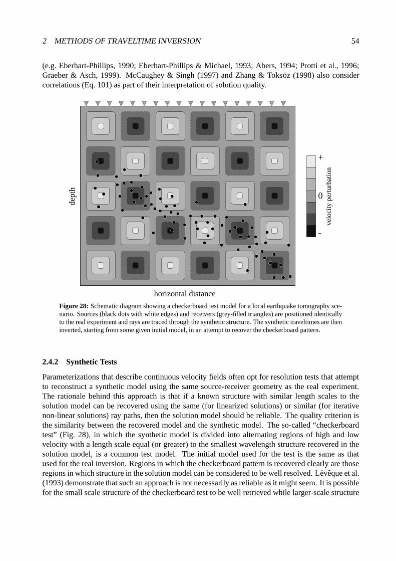
2 METHODS OF TRAVELTIME INVERSION 54
(e.g. Eberhart-Phillips, 1990; Eberhart-Phillips & Michael, 1993; Abers, 1994; Protti et al., 1996;Graeber & Asch, 1999). McCaughey & Singh (1997) and Zhang & Toksoz (1998) also considercorrelations (Eq. 101) as part of their interpretation of solution quality.
velo
city
per
turb
atio
n
0
-
+
dept
h
horizontal distance
Figure 28: Schematic diagram showing a checkerboard test model for a local earthquake tomography sce-nario. Sources (black dots with white edges) and receivers (grey-filled triangles) are positioned identicallyto the real experiment and rays are traced through the synthetic structure. The synthetic traveltimes are theninverted, starting from some given initial model, in an attempt to recover the checkerboard pattern.
2.4.2 Synthetic Tests
Parameterizations that describe continuous velocity fields often opt for resolution tests that attemptto reconstruct a synthetic model using the same source-receiver geometry as the real experiment.The rationale behind this approach is that if a known structure with similar length scales to thesolution model can be recovered using the same (for linearized solutions) or similar (for iterativenon-linear solutions) ray paths, then the solution model should be reliable. The quality criterion isthe similarity between the recovered model and the synthetic model. The so-called “checkerboardtest” (Fig. 28), in which the synthetic model is divided into alternating regions of high and lowvelocity with a length scale equal (or greater) to the smallest wavelength structure recovered in thesolution model, is a common test model. The initial model used for the test is the same as thatused for the real inversion. Regions in which the checkerboard pattern is recovered clearly are thoseregions in which structure in the solution model can be considered to be well resolved. Leveque et al.(1993) demonstrate that such an approach is not necessarily as reliable as it might seem. It is possiblefor the small scale structure of the checkerboard test to be well retrieved while larger-scale structure
3 APPLICATIONS TO OBSERVED DATA 55
is poorly retrieved. Furthermore, if the solution takes into account the non-linearity of the inverseproblem, then the ray-path coverage will have a dependence on the velocity distribution. Thus,while a checkerboard reconstruction can account for the non-linearity of the traveltime dependenceon the checkerboard structure, it cannot account for the non-linearity of the traveltime dependenceon the true structure. Thus, rather than iteratively invert for the checkerboard structure, it may bebetter to simply use the ray-path geometry from the model produced by the inversion of the realdata in a linear inversion. Alternatively, one could test a number of different synthetic models toinvestigate the effect of different structures (and hence ray geometries) on the resolution; this wouldbe advisable especially if the solution model is complex.
Teleseismic traveltime tomography studies that have used checkerboard resolution tests includethose by Glahn & Granet (1993), Achauer (1994) and Seber et al. (1996). Ritsema et al. (1998)used several different synthetic models rather than checkerboards and analyzed the accuracy of theirrecovery. This kind of analysis is not commonly used in wide-angle studies, although recently, Zelt(1998), Zelt et al. (1999, 2001) and Day et al. (2001) implemented checkerboard tests for analyzingthe resolution of velocity structure (Zelt et al., 1999, also use it for interface structure) derived fromwide-angle traveltime inversion. In local earthquake tomography, checkerboard tests have beenimplemented by Chiarabba et al. (1997) and Graeber & Asch (1999); Walck & Clayton (1987) andWalck (1988) used synthetic reconstructions with anomalies positioned in key localities (i.e. regionsof high geological interest).
3 Applications to Observed Data
In this section, we review some applications of traveltime inversion methods to real data. Our aim isto give an idea of how the methods described above can be put together to solve a 2-D or 3-D inverseproblem in practice. With this is mind, we tend to focus our attention on several selected case studies,rather than just briefly describe numerous examples. The choice of which methods to use is usuallyinfluenced by the class of data (reflection, wide-angle, local earthquake, teleseismic) that is available(see Section 1.3). For example, normal incidence reflection data, as its name suggests, predominantlycontains reflected phases, so interfaces must be included in the parameterization. Teleseismic data,on the other hand, do not contain reflected phases, so structure in this case is generally representedby a continuous velocity variation. Thus, the different data types often resolve different aspects ofstructure, a feature that will also be discussed in some detail below.
3.1 Reflection Tomography
A number of 2-D schemes for the tomographic interpretation of reflection data have been presentedover the years but not many of them have been extensively applied to real data (at least, there arenot many examples in the literature). Bishop et al. (1985) presented one of the first methods forthe simultaneous determination of velocity and depth in laterally varying media. In their method,the subsurface is represented by sub-horizontal layers separated by interfaces with a cubic splineparameterization. Within each layer, velocity is permitted to vary laterally and vertically by meansof a grid of constant velocity gradient boxes. Within each box, a ray path segment will have thegeometry of a circular arc, and therefore has an analytic expression. A shooting method of raytracing determines source-receiver ray paths and traveltimes, and a Gauss-Newton method is usedto iteratively minimize an objective function consisting of a data residual term and a model length
3 APPLICATIONS TO OBSERVED DATA 56
term (i.e. damping but no smoothing). The system of linear equations is solved using a Gauss-Seidel algorithm with successive over-relaxation. The method was applied to Common Depth Point(CDP) data from a pair of intersecting profiles in a region with permafrost. Significant shallowvelocity variations due to the presence of the permafrost were imaged and the depth estimates tothe interfaces at the intersection of the profiles agreed significantly better that those determined byconventional seismic processing. The maximum depth to which structure was imaged was ∼5.5 km.
It has been recognized by a number of authors that reflection traveltimes poorly resolve verticalvariations of velocity within a layer (Farra & Madariaga, 1988; Kosloff et al., 1996). In the methodof Farra & Madariaga (1988), a layered parameterization is adopted in which interfaces and lateralvelocity variations within layers are described by cubic B-splines. Velocity within a layer is verti-cally invariant. Source-receiver ray paths and traveltimes are found with a shooting method of raytracing that uses elements of paraxial ray theory to iteratively correct the ray take-off angle. The ob-jective function they minimize consists of a data residual term and a penalty function which restrictsthe model behavior in accordance with the available a priori model information. A DLS approach isapplied to iteratively minimize the objective function, and SVD is used to solve the system of linearequations at each step. They also make use of a layer-stripping approach. In this scheme, reflectiontraveltimes from the top interface are initially used to constrain the top layer only. Once these dataare satisfied, traveltimes for the second interface are also introduced and together they are used toconstrain the first two layers. The scheme continues in this manner through each successive layer.Farra & Madariaga (1988) applied their scheme to a synthetic model that included a layer pinchout,and showed that it can be reconstructed using a model with 1-D structure as a starting model. Cou-pled oscillations of interfaces and velocity variations were found to occur in regions where the datawere unable to resolve the trade-off between interface depth variation and lateral velocity variationwithin a layer. They then applied the scheme to data from the Paris Basin. The maximum offsetbetween source and receiver was 1.68 km, and structure was imaged to a depth of 2 km. A totalof 99 parameters (57 velocity, 42 interface) were used to describe the model. The initial modelwas described by four flat constant velocity layers. In the solution model, the interfaces remainednearly horizontal, but the layer velocities had significant lateral variations. The recovered interfacegeometries are consistent with the known structure of the region.
Imaging of 3-D structure by reflection tomography is not very common. Chiu et al. (1986)developed and applied a scheme to vibroseis data collected on Vancouver Island. Their methodassumes that subsurface structure can be adequately represented by constant velocity layers thatseparate interfaces described by nth-order polynomial surfaces. A ray bending scheme is used tosolve the forward problem, and an iterative damped least squares approach is used to solve the inverseproblem. As in the above methods the linear system of equations are solved with SVD. However, intheir application to crooked line vibroseis data collected as part of PROJECT LITHOPROBE, only110 traveltime picks were available to constrain the structure of a two-interface model, consistingof a decollement zone and an under-thrusting oceanic crust. They found that planar interfaces wereadequate to satisfy the data, making this a rather limited example of 3-D tomography.
In general, coincident reflection traveltime data alone do not seem to be sufficient to resolve bothinterface depth variations and arbitrary velocity variations within a layer, despite the relatively denseray coverage associated with most reflection experiments. Williamson (1990) confirms this limita-tion by using a multi-stage inversion scheme in which progressively shorter length scales are per-mitted in both velocity and interface geometry as the iterative process proceeds. Despite satisfyingthe data and finding that longer wavelength components may be adequately recovered, Williamson

3 APPLICATIONS TO OBSERVED DATA 57
(1990) also found that shorter wavelength velocity-depth trade-offs cannot be resolved without fur-ther information. This may take the form of a priori information to help constrain the problem,and/or simplifying assumptions made about the structure (e.g. constant velocity layers, layers inwhich velocity has no vertical variation). While this may be sufficient at shallow depths, a basicdrawback of reflection tomography is that the resolving power of the data decreases with depth dueto the geometry of the experiment. Thus, it is usually limited to near-surface applications.
3.2 Wide-Angle Tomography
Unlike coincident reflection tomography, inversion of wide-angle traveltimes for 2-D or 3-D crustalstructure has been applied to many datasets from around the world. For example, numerous studieshave been carried out in Canada (e,g, Hole et al., 1992; Kanasewich et al., 1994; Clowes et al., 1995;Zelt & White, 1995; Morozov et al., 1998; Zelt et al., 2001), the U.S. (e.g. Lutter & Nowack, 1990;Jarchow et al., 1994; Zhu & Ebel, 1994; Parsons et al., 1996; Wang & Braile, 1996; Lizarralde &Holbrook, 1997), Europe (e.g. Riahi & Lund, 1994; Staples et al., 1997; Darbyshire et al., 1998;Louden & Fan, 1998; Mjelde et al., 1998; Korenaga et al., 2000; Morgan et al., 2000) and in oceanicsettings (e.g. Hildebrand et al., 1989; Wiggins et al., 1996; Kodaira et al., 1998; Recq et al., 1998;Day et al., 2001; Grevemeyer et al., 2001). Experiments involving marine air-gun sources and landbased receivers or OBSs (Ocean Bottom Seismometers) are quite common since they can be cou-pled with coincident reflection studies. As discussed in Section 1.3, wide-angle data contain bothrefraction and wide-angle reflection phases. The traveltimes of rays that refract tend to constrain ve-locity variations better than wide-angle reflections, which in turn are better at constraining interfacedepth. Thus, with adequate data coverage, the simultaneous inversion of refraction and reflectiontraveltimes can result in a well constrained solution model that includes both variations in interfacedepth and layer velocity.
Wide-angle experiments are usually performed in 2-D (i.e. recorded by an in-line array of sourcesand receivers), although recent studies (Zelt & Barton, 1998; Zelt et al., 1999; Day et al., 2001;Rawlinson et al., 2001b; Zelt et al., 2001) indicate that 3-D wide-angle surveys are becoming morefrequent. In 2-D experiments, data coverage is often quite dense, and tomographic-style interpre-tation techniques are usually designed to allow both interface structure and layer velocities to beconstrained by the data. One of the most frequently used methods for the tomographic style inver-sion of 2-D wide-angle traveltimes was developed by Zelt & Smith (1992). In their method, themodel is parameterized in terms of a layered network of irregular blocks (see Section 2.1), whichallows velocity to vary both laterally and vertically within a layer. Layer pinchouts and isolatedbodies can also be included by reducing layer thickness to zero. The advantage of this approach tostructural representation is that velocity and interface node distribution can be adapted to suit theresolving power of the dataset. Refractions, reflections and head waves are traced through the modelby numerically solving the initial value problem formulated in terms of a pair of first order ordinarydifferential equations (Eq. 19 and Eq. 20). Linear interpolation between rays that bracket a given re-ceiver is used to estimate the corresponding traveltime and Frechet derivatives. The inverse problemis solved using an iterative DLS method (damping but no smoothing), with rays re-traced after eachiteration. LU decomposition is used to solve the system of linear equations.
A number of authors have adopted the approach of Zelt & Smith (1992) to invert wide-angledata, including Kanasewich et al. (1994), Riahi & Juhlin (1994), Staples et al. (1997), Ye et al.(1997), Darbyshire et al. (1998), Kodaira et al. (1998), Morozov et al. (1998) and Navin et al.(1998). Darbyshire et al. (1998) applied it to data from the ICEMELT refraction line to image crustal

3 APPLICATIONS TO OBSERVED DATA 58
Figure 29: Crustal model obtained from the ICEMELT refraction line in Iceland using the wide-angletraveltime inversion method of Zelt & Smith (1992). Solid lines on the Moho represent those parts of theinterface constrained by the data. [From Darbyshire et al. (1998). Copyright 1998 Royal AstronomicalSociety. Reproduced by permission of Blackwell Science Ltd.]
structure above the Iceland mantle plume. In their study, up to 60 land-based recorders were usedto record seismic energy from six explosive shots along a 310 km line traversing Iceland from northto south. A total of 181 traveltime picks were used to constrain the crustal model, which includedboth interfaces and velocity variations within a layer. The inversion solution produced a normalizedχ2 misfit value of 1.31. Fig. 29 shows the ICEMELT crustal model produced by the inversion ofrefraction and wide-angle reflection traveltimes. The upper crust is characterized by high verticalvelocity gradients (>0.2 s−1) and considerable lateral heterogeneity. By contrast, the lower crust isless complex and features much smaller vertical velocity gradients (<0.03 s−1). The crust thickensto nearly 40 km depth above the mantle plume, a feature interpreted to be caused by increased meltgeneration due to elevated mantle temperatures and active convection in the plume core. Two of themethods used by Darbyshire et al. (1998) to analyze the robustness of their solution model are raycoverage and estimates of resolution from linear theory. Fig. 30a shows all the ray paths used toconstrain the ICEMELT model, and Fig. 30b shows a plot of the diagonal elements of the resolutionmatrix; values ≥ 0.5 are considered well resolved. Several regions in the upper and lower crust arepoorly resolved while the mid crust is generally well resolved.
Darbyshire et al. (1998) did not use the inversion routine of Zelt & Smith (1992) in a completelyautomated fashion. Manual intervention (i.e. the user empirically tunes one or more parameter valuesinstead of the inversion routine) was used to refine some of the upper crustal structure. In 2-Dwide-angle modeling, it is sometimes necessary to intervene during the inversion process to preventunrealistic model perturbations caused, for example, by insufficient data constraints or extreme non-linearity. In some studies (e.g. Iwasaki et al., 1990; Gurbuz & Evans, 1991; Grad et al., 1997; Iwasakiet al., 1998; Recq et al., 1998), the inversion is performed completely manually in a process called“forward modeling” (i.e. one tries to satisfy the data by adjusting model parameter values using trial

3 APPLICATIONS TO OBSERVED DATA 59
(a)
(b)
Figure 30: (a) All ray paths used to constrain the model in Fig. 29 and (b) diagonal elements of the reso-lution matrix obtained from linear theory. Regions that are considered well constrained have a value ≥0.5.[From Darbyshire et al. (1998). Copyright 1998 Royal Astronomical Society. Reproduced by permissionof Blackwell Science Ltd.]
and error). The advantage of this approach is that the user has complete control over the state of themodel, and that hypothetical structures may be tested against the data. On the other hand, if thereare a large number of model parameters, repeated forward modeling becomes very time consuming.
Wide-angle seismic studies that attempt to constrain structure in 3-D usually do not consider bothinterface structure and layer velocity variations. For example, Hole (1992), Hammer et al. (1994),Toomey et al. (1994), Zelt & Barton (1998), Day et al. (2001) and Zelt et al. (2001) inverted firstarrivals for continuously varying velocity, and Hole et al. (1992) and Riahi & Juhlin (1994) invertedrefraction and reflection traveltimes respectively for interface structure. Studies that have attemptedto invert for both parameter types include Zelt et al. (1996), who use a layer stripping approach,and Zelt (1999), who use floating reflectors coupled with sharp velocity gradients to simulate dis-continuities. Most of the above 3-D wide-angle studies use methods to solve the forward problemof traveltime and ray path determination based on the finite difference approach of Vidale (1990).
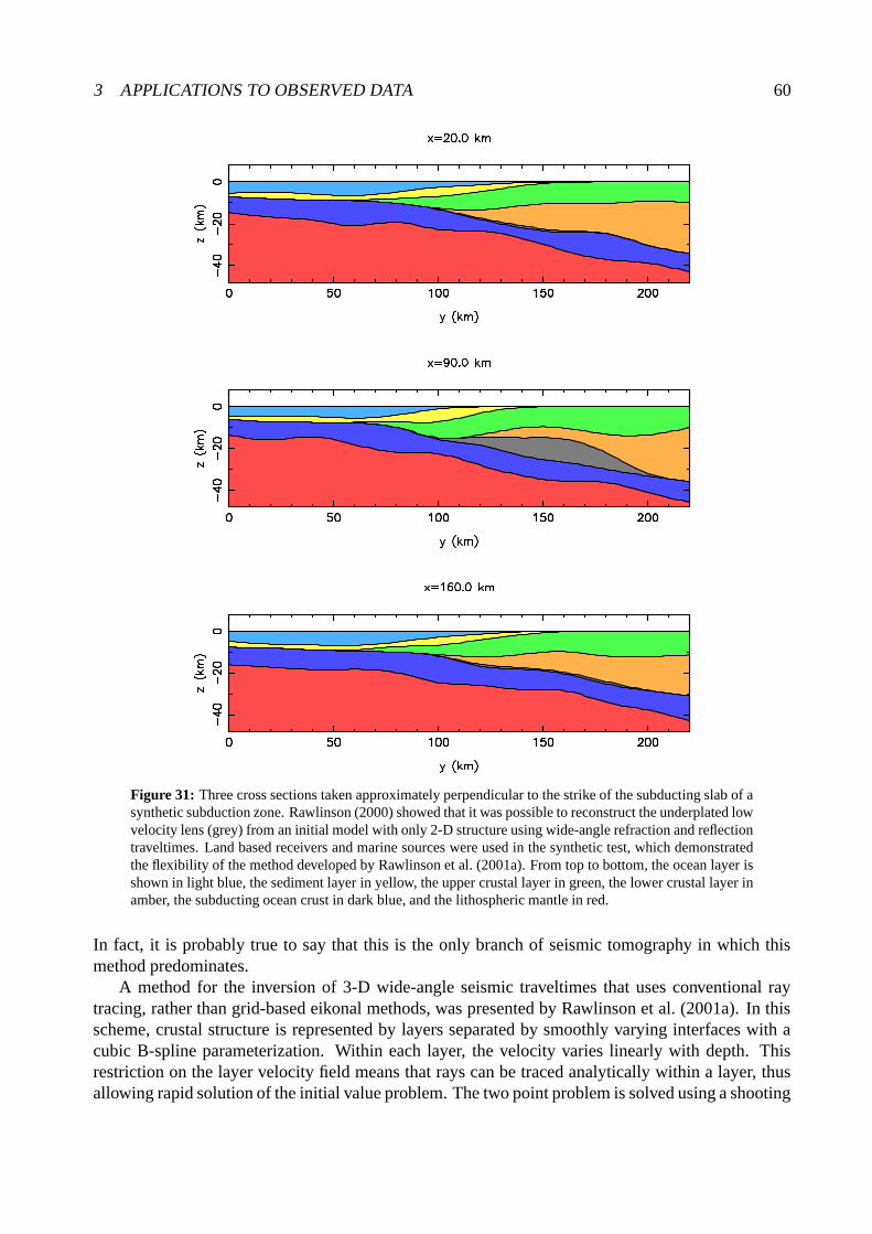
3 APPLICATIONS TO OBSERVED DATA 60
Figure 31: Three cross sections taken approximately perpendicular to the strike of the subducting slab of asynthetic subduction zone. Rawlinson (2000) showed that it was possible to reconstruct the underplated lowvelocity lens (grey) from an initial model with only 2-D structure using wide-angle refraction and reflectiontraveltimes. Land based receivers and marine sources were used in the synthetic test, which demonstratedthe flexibility of the method developed by Rawlinson et al. (2001a). From top to bottom, the ocean layer isshown in light blue, the sediment layer in yellow, the upper crustal layer in green, the lower crustal layer inamber, the subducting ocean crust in dark blue, and the lithospheric mantle in red.
In fact, it is probably true to say that this is the only branch of seismic tomography in which thismethod predominates.
A method for the inversion of 3-D wide-angle seismic traveltimes that uses conventional raytracing, rather than grid-based eikonal methods, was presented by Rawlinson et al. (2001a). In thisscheme, crustal structure is represented by layers separated by smoothly varying interfaces with acubic B-spline parameterization. Within each layer, the velocity varies linearly with depth. Thisrestriction on the layer velocity field means that rays can be traced analytically within a layer, thusallowing rapid solution of the initial value problem. The two point problem is solved using a shooting
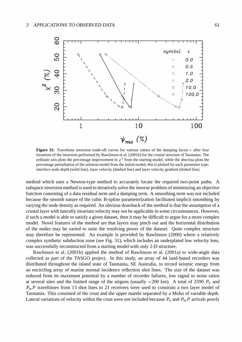
3 APPLICATIONS TO OBSERVED DATA 61
Figure 32: Traveltime inversion trade-off curves for various values of the damping factor ε after fouriterations of the inversion performed by Rawlinson et al. (2001b) for the crustal structure of Tasmania. Theordinate axis plots the percentage improvement in χ 2 from the starting model, while the abscissa plots thepercentage perturbation of the solution model from the initial model; this is plotted for each parameter type:interface node depth (solid line), layer velocity (dashed line) and layer velocity gradient (dotted line).
method which uses a Newton-type method to accurately locate the required two-point paths. Asubspace inversion method is used to iteratively solve the inverse problem of minimizing an objectivefunction consisting of a data residual term and a damping term. A smoothing term was not includedbecause the smooth nature of the cubic B-spline parameterization facilitated implicit smoothing byvarying the node density as required. An obvious drawback of the method is that the assumption of acrustal layer with laterally invariant velocity may not be applicable in some circumstances. However,if such a model is able to satisfy a given dataset, then it may be difficult to argue for a more complexmodel. Novel features of the method are that layers may pinch out and the horizontal distributionof the nodes may be varied to suite the resolving power of the dataset. Quite complex structuremay therefore be represented. An example is provided by Rawlinson (2000) where a relativelycomplex synthetic subduction zone (see Fig. 31), which includes an underplated low velocity lens,was successfully reconstructed from a starting model with only 2-D structure.
Rawlinson et al. (2001b) applied the method of Rawlinson et al. (2001a) to wide-angle datacollected as part of the TASGO project. In this study, an array of 44 land-based recorders wasdistributed throughout the island state of Tasmania, SE Australia, to record seismic energy froman encircling array of marine normal incidence reflection shot lines. The size of the dataset wasreduced from its maximum potential by a number of recorder failures, low signal to noise ratiosat several sites and the limited range of the airguns (usually <200 km). A total of 2590 Pn andPm P traveltimes from 13 shot lines to 21 receivers were used to constrain a two layer model ofTasmania. This consisted of the crust and the upper mantle separated by a Moho of variable depth.Lateral variations of velocity within the crust were not included because Pn and Pm P arrivals poorly
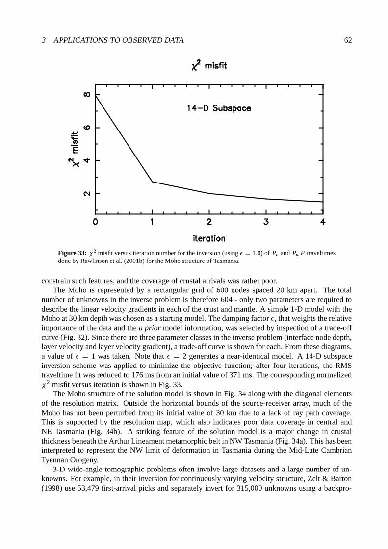
3 APPLICATIONS TO OBSERVED DATA 62
Figure 33: χ2 misfit versus iteration number for the inversion (using ε = 1.0) of Pn and Pm P traveltimesdone by Rawlinson et al. (2001b) for the Moho structure of Tasmania.
constrain such features, and the coverage of crustal arrivals was rather poor.The Moho is represented by a rectangular grid of 600 nodes spaced 20 km apart. The total
number of unknowns in the inverse problem is therefore 604 - only two parameters are required todescribe the linear velocity gradients in each of the crust and mantle. A simple 1-D model with theMoho at 30 km depth was chosen as a starting model. The damping factor ε, that weights the relativeimportance of the data and the a prior model information, was selected by inspection of a trade-offcurve (Fig. 32). Since there are three parameter classes in the inverse problem (interface node depth,layer velocity and layer velocity gradient), a trade-off curve is shown for each. From these diagrams,a value of ε = 1 was taken. Note that ε = 2 generates a near-identical model. A 14-D subspaceinversion scheme was applied to minimize the objective function; after four iterations, the RMStraveltime fit was reduced to 176 ms from an initial value of 371 ms. The corresponding normalizedχ2 misfit versus iteration is shown in Fig. 33.
The Moho structure of the solution model is shown in Fig. 34 along with the diagonal elementsof the resolution matrix. Outside the horizontal bounds of the source-receiver array, much of theMoho has not been perturbed from its initial value of 30 km due to a lack of ray path coverage.This is supported by the resolution map, which also indicates poor data coverage in central andNE Tasmania (Fig. 34b). A striking feature of the solution model is a major change in crustalthickness beneath the Arthur Lineament metamorphic belt in NW Tasmania (Fig. 34a). This has beeninterpreted to represent the NW limit of deformation in Tasmania during the Mid-Late CambrianTyennan Orogeny.
3-D wide-angle tomographic problems often involve large datasets and a large number of un-knowns. For example, in their inversion for continuously varying velocity structure, Zelt & Barton(1998) use 53,479 first-arrival picks and separately invert for 315,000 unknowns using a backpro-

3 APPLICATIONS TO OBSERVED DATA 63
TFS
TFS
a b
AL
AL
Figure 34: (a) Moho depth and (b) diagonal elements of the resolution matrix of the solution model forTasmania produced from the TASGO wide-angle dataset. In both diagrams, stars indicate recorders andsmall triangles indicate shot points from which data were picked. Contiguous triangles form shot linesexcept where data gaps occur (e.g. lines 4 and 15). Thick dashed lines denote tectonic element boundaries:Arthur Lineament (AL) and Tamar Fracture System (TFS). [From Rawlinson et al. (2001b). Copyright2001 American Geophysical Union. Reproduced by permission of American Geophysical Union]
jection method and 35,000 unknowns using a regularized least squares method. Studies of a similarmagnitude were recently carried out by Day et al. (2001) and Zelt et al. (2001).
In summary, wide-angle tomography has proven to be a useful tool for revealing informationabout crustal structure. Its strength is its ability to resolve the trade-off between interface depthand lateral velocity variation within a layer given sufficient data coverage. This is in contrast tocoincident reflection tomography. The main weaknesses of wide-angle tomography are the difficultyof picking reflection phases, which are always later arrivals, and the presence of extreme lateralvariations in crustal structure, which can cause significant ray-path perturbations, and hence violatethe local linearity assumption upon which iterative inversion methods are based.
3.3 Local Earthquake Tomography
Local earthquake tomography (LET) is a common tool for imaging subsurface structure in seismi-cally active areas. Studies have been carried out in many different regions including California (Aki& Lee, 1976; Thurber, 1983; Eberhart-Phillips, 1986; Walck & Clayton, 1987; Walck, 1988; Zhao& Kanamori, 1992; Eberhart-Phillips & Michael, 1993; Scott et al., 1994), Taiwan (Kao & Rau,1999), Japan (Nakanishi, 1985; Zhao et al., 1992), South America (Bosch, 1997; Graeber & Asch,1999) and the Mediterranean (Chiarabba et al., 1997; Luca et al., 1997; Papazachos & Nolet, 1997;Haslinger et al., 1999). Apart from the source-receiver geometry, one of the distinguishing featuresof LET compared to the other types of tomography discussed here, is the need to relocate earthquake
3 APPLICATIONS TO OBSERVED DATA 64
hypocenters (spatial location and origin time) as part of the image reconstruction. This is becauseaccurate hypocenter location requires an accurate knowledge of the velocity structure in the regionoccupied by the earthquakes and the recorders whose data are used in the location process. Adequatedata are therefore required to resolve the trade-off between variations in structure and variations inhypocenter locations.
One of the original LET studies was carried out by Aki & Lee (1976). In their method, 3-D crustal structure is represented by constant slowness blocks. The initial model is completelyhomogeneous, and the inversion is linear, so rays consist of straight line paths between sourcesand receivers. Slowness perturbations for each block and hypocenter corrections are simultaneouslyinverted for using a DLS approach (damping but no smoothing). The method was applied to datacollected at 60 stations in Bear Valley, California, from 32 local earthquakes. The x × y × z blocksize was set at 3 × 4 × 5 km3, with a total of 264 blocks used to span a volume of 24 × 44 × 15 km3
which included all receivers and sources. 1218 first-arrival times were inverted for all unknowns.Estimates of covariance and resolution from linear theory were used to analyze the robustness of thevelocity solution and relocated hypocenters. A feature of the solution model is a narrow low velocityband oriented along the San Andreas fault zone in the upper 5 km.
The conceptual basis of LET has not really altered since the study of Aki & Lee (1976). However,some refinements have been made. For example, Thurber (1983) used approximate 3-D ray tracing(which allows iterative improvement of the solution model) and a continuously varying velocity fieldvia linear interpolation of a uniform grid of velocity nodes. Eberhart-Phillips (1990) introduced apseudo bending scheme to find more accurate two-point paths starting from rays calculated usingthe approximate ray tracing method of Thurber (1983). These refinements are common to most im-plementations of LET in recent times and are encapsulated in the commonly used computer packageSIMULPS12 (Evans et al., 1994).
A relatively recent application of LET was carried out by Graeber & Asch (1999) to image thesubduction zone structure beneath the southern central Andes. In this study, local earthquakes wererecorded by a network of 31 recorders deployed in northern Chile between the Coastal Cordillera andthe Western Cordillera. A total of 16,488 P-arrivals from 764 events were inverted for P-velocitystructure and hypocenter location using the SIMULPS12 algorithm. The initial model required bythe inversion scheme was based upon a model produced by a separate inversion of the data for 1-D structure and hypocenter location only. The optimum damping factor for the DLS solution wasobtained by visual inspection of the data variance vs. solution variance trade-off curve approximatedby performing several single-iteration inversions with a range of damping values. Station delay termswere also included in the inversion as unknowns to help offset the effects of near surface structure.The solution model was obtained after 12 iterations of the DLS method, which reduced the datavariance by 63% with respect to the optimum 1-D model. Fig. 35 shows a series of vertical slicesthrough the resulting P-wave velocity model, which is described by a total of 2496 nodes. Relocatedhypocenters are also shown in this figure. Only those parts of the velocity model that are relativelywell resolved according to the diagonal elements of the resolution matrix are shown in Fig. 35. Thesolution model clearly suggests the presence of a subduction zone involving the easterly subductionof oceanic crust beneath continental crust, with the geometry of the subducted plate also indicatedby the relocated hypocenters.
Apart from calculating the resolution matrix to investigate solution robustness, Graeber & Asch(1999) also performed several synthetic resolution tests, including a checkerboard test. The resultsof this test at two cross-sections are shown in Fig. 36. As expected, the reconstruction below the

3 APPLICATIONS TO OBSERVED DATA 65
6.5
8
8.5
0
50
100
150
DE
PT
H [k
m]
70˚W 69˚W 68˚W 67˚W
W E
22.25˚S
4.5 5.0 5.5 6.0 6.5 7.0 7.5 8.0 8.5 9.0
Vp [km/s]
6
6.5
6.5 6.5
7
7
7
7.5
88
0
50
100
150
DE
PT
H [k
m]
70˚W 69˚W 68˚W 67˚W
W E
22.75˚S
4.5 5.0 5.5 6.0 6.5 7.0 7.5 8.0 8.5 9.0
Vp [km/s]
6
6
6.5
6.57
7
7.5
8
9
0
50
100
150
DE
PT
H [k
m]
70˚W 69˚W 68˚W 67˚W
W E
23.25˚S
4.5 5.0 5.5 6.0 6.5 7.0 7.5 8.0 8.5 9.0
Vp [km/s]
Figure 35: Cross-sections through a 3-D velocity model of the southern central Andes produced by in-version of local earthquake arrival times. Absolute velocities shown are a sum of initial velocities andcalculated perturbations from an iterative non-linear inversion technique. Stations, recent volcanos andhypocenters adjacent to the sections are denoted by squares, triangles and open circles respectively. Velocitygrid nodes are denoted by crosses. [From Graeber & Asch (1999). Copyright 1999 American GeophysicalUnion. Reproduced by permission of American Geophysical Union]
hypocenters is generally poor, but in the region between the hypocenters and receivers the recon-struction is generally good.
In addition to using first-arrival P-wave data, it is also quite common in LET to utilize S-wavedata. A particularly useful property to map is the P-to-S velocity ratio (Vp/Vs). For example,regions with high levels of hydration are likely to have elevated Vp/Vs since the shear modulus willbe reduced compared to the bulk modulus. One way of determining Vp/Vs is to separately invert forP and S velocity structure and then compare the results (e.g. Eberhart-Phillips, 1990). One problemwith this is that the S-wave dataset is often smaller and of poorer quality than the P-wave dataset,
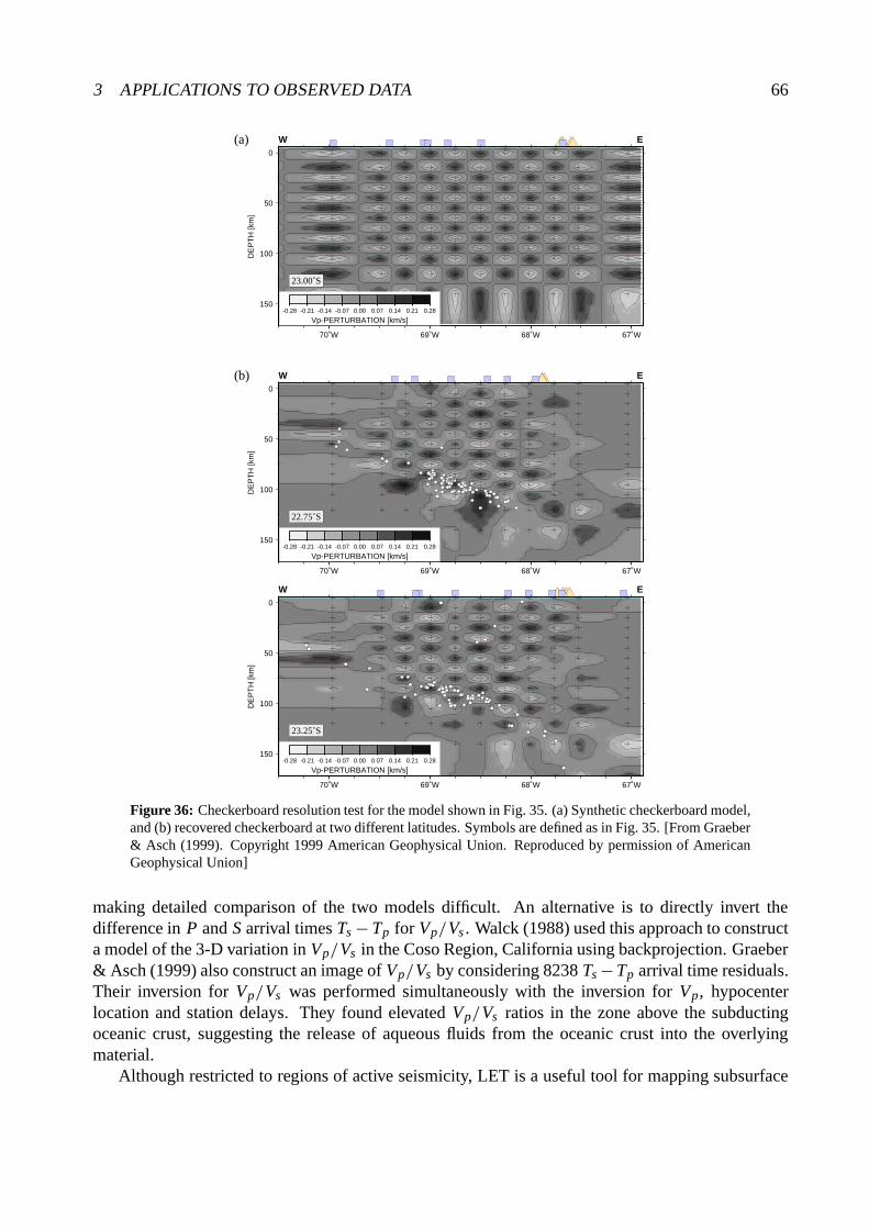
3 APPLICATIONS TO OBSERVED DATA 66
0
50
100
150
DE
PT
H [k
m]
70˚W 69˚W 68˚W 67˚W
W E
23.00˚S
-0.28 -0.21 -0.14 -0.07 0.00 0.07 0.14 0.21 0.28
Vp-PERTURBATION [km/s]
0
50
100
150
DE
PT
H [k
m]
70˚W 69˚W 68˚W 67˚W
W E
22.75˚S
-0.28 -0.21 -0.14 -0.07 0.00 0.07 0.14 0.21 0.28
Vp-PERTURBATION [km/s]
0
50
100
150
DE
PT
H [k
m]
70˚W 69˚W 68˚W 67˚W
W E
23.25˚S
-0.28 -0.21 -0.14 -0.07 0.00 0.07 0.14 0.21 0.28
Vp-PERTURBATION [km/s]
(a)
(b)
Figure 36: Checkerboard resolution test for the model shown in Fig. 35. (a) Synthetic checkerboard model,and (b) recovered checkerboard at two different latitudes. Symbols are defined as in Fig. 35. [From Graeber& Asch (1999). Copyright 1999 American Geophysical Union. Reproduced by permission of AmericanGeophysical Union]
making detailed comparison of the two models difficult. An alternative is to directly invert thedifference in P and S arrival times Ts − Tp for Vp/Vs . Walck (1988) used this approach to constructa model of the 3-D variation in Vp/Vs in the Coso Region, California using backprojection. Graeber& Asch (1999) also construct an image of Vp/Vs by considering 8238 Ts − Tp arrival time residuals.Their inversion for Vp/Vs was performed simultaneously with the inversion for Vp, hypocenterlocation and station delays. They found elevated Vp/Vs ratios in the zone above the subductingoceanic crust, suggesting the release of aqueous fluids from the oceanic crust into the overlyingmaterial.
Although restricted to regions of active seismicity, LET is a useful tool for mapping subsurface

3 APPLICATIONS TO OBSERVED DATA 67
structure at a variety of scales. Shallow earthquakes can be used to image the upper few kilometersof the crust (e.g. Walck, 1988; Chiarabba et al., 1997) while deep earthquakes from regions like sub-duction zones can be used to image lithospheric scale structure (e.g. Graeber & Asch, 1999). Whilerelocation of earthquake hypocenters is a necessary part of the reconstruction of the velocity fieldfrom the data, their distribution provides valuable additional information on subsurface structure.Inclusion of S-wave data in the form of inversion of Ts − Tp for Vp/Vs is not commonly consideredin the other forms of tomography described in this paper, further distinguishing LET as a methodworth considering provided local earthquake sources are available.
3.4 Teleseismic Tomography
Like wide-angle tomography and local earthquake tomography, teleseismic tomography has beenused extensively to map the structure of the crust and lithosphere. Studies are often carried outon a variety of scales ranging from 10s of km (e.g. Rawlinson & Houseman, 1998; Steck et al.,1998) to 100s of km (e.g. Humphreys & Clayton, 1990; Dorbath & Paul, 1996). In the latter type ofstudy, mantle beneath the lithosphere is also imaged. Usually, the horizontal extent of the receiverarray and the source distribution determines the depth to which features may be resolved. Mostteleseismic studies are carried out in 3-D (e.g. Aki et al., 1977; Oncescu et al., 1984; Humphreys &Clayton, 1990; Benz et al., 1992; Glahn & Granet, 1993; Achauer, 1994; Seber et al., 1996; Saltzer& Humphreys, 1997; Ritsema et al., 1998; Steck et al., 1998; Graeber et al., 2002), with relativelyfew 2-D studies (e.g. Evans, 1982; McQueen & Lambeck, 1996) probably because of the difficultyin lining up an array of recorders on roughly the same great circle as a set of teleseismic earthquakeswith good angular coverage.
The data utilized by teleseismic tomography studies are the relative traveltime residuals of identi-fiable phases (usually the direct P-phase). These are obtained by calculating the difference betweenpredicted and observed traveltimes and subtracting the mean for each source-receiver set. Predictedtraveltimes are usually obtained by ray tracing through a 1-D reference model of the Earth, suchas IASP91 (Kennett & Engdahl, 1991). Removing the mean from each set of traveltime residualsmeans that they are relatively insensitive to errors in hypocenter location. However, they also be-come insensitive to vertical variations in structure. One consequence of this is that the horizontallyaveraged velocity structure of the solution model will simply reflect the horizontally averaged veloc-ity structure of the initial model. Interpretation of the resulting models must therefore be done withcare (see Leveque & Masson, 1999, for more details).
One of the first papers to describe a method of seismic tomography was that of Aki et al. (1977),who developed a scheme in the context of application to teleseismic data. In their method, thelithosphere is represented by layers composed of constant velocity blocks. Incoming wavefrontsfrom teleseismic events are assumed to be locally planar beneath the model region and the initialmodel has constant velocity layers. Thus, the task of ray tracing from the incident wavefront to thereceiver array is straightforward. Linear inversion is performed using either a stochastic inverse ora generalized inverse approach. The stochastic solution is essentially a DLS solution with ε = 1,while the generalized inverse solution has ε = 0, but identifies a minimum length solution usingSVD. The method was applied to data collected by the Norwegian Seismic Array (Norsar) to imagelithospheric structure in southeastern Norway. A total of 1496 traveltime residuals from 93 eventsrecorded at 22 sites (each consisting of six seismometers) were inverted for the slowness perturbationof 405 constant velocity blocks contained in a five-layer model of the lithosphere (9 × 9 blocks perlayer). The model region has a horizontal coverage of 180 × 180 km and extends to a depth of 126
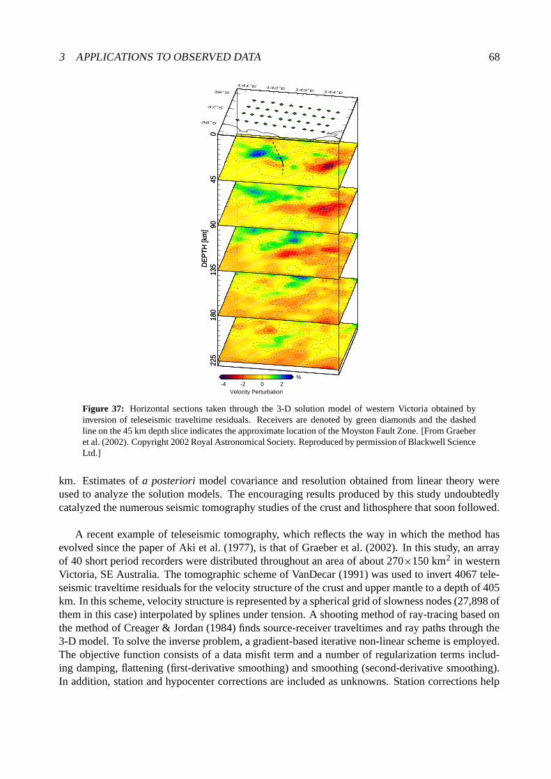
3 APPLICATIONS TO OBSERVED DATA 68
045
9013
518
022
5D
EP
TH [k
m]
045
9013
518
022
5D
EP
TH [k
m]
-4 -2 0 2Velocity Perturbation
%
141˚E 142˚E 143˚E 144˚E
38˚S
37˚S
36˚S
Figure 37: Horizontal sections taken through the 3-D solution model of western Victoria obtained byinversion of teleseismic traveltime residuals. Receivers are denoted by green diamonds and the dashedline on the 45 km depth slice indicates the approximate location of the Moyston Fault Zone. [From Graeberet al. (2002). Copyright 2002 Royal Astronomical Society. Reproduced by permission of Blackwell ScienceLtd.]
km. Estimates of a posteriori model covariance and resolution obtained from linear theory wereused to analyze the solution models. The encouraging results produced by this study undoubtedlycatalyzed the numerous seismic tomography studies of the crust and lithosphere that soon followed.
A recent example of teleseismic tomography, which reflects the way in which the method hasevolved since the paper of Aki et al. (1977), is that of Graeber et al. (2002). In this study, an arrayof 40 short period recorders were distributed throughout an area of about 270×150 km2 in westernVictoria, SE Australia. The tomographic scheme of VanDecar (1991) was used to invert 4067 tele-seismic traveltime residuals for the velocity structure of the crust and upper mantle to a depth of 405km. In this scheme, velocity structure is represented by a spherical grid of slowness nodes (27,898 ofthem in this case) interpolated by splines under tension. A shooting method of ray-tracing based onthe method of Creager & Jordan (1984) finds source-receiver traveltimes and ray paths through the3-D model. To solve the inverse problem, a gradient-based iterative non-linear scheme is employed.The objective function consists of a data misfit term and a number of regularization terms includ-ing damping, flattening (first-derivative smoothing) and smoothing (second-derivative smoothing).In addition, station and hypocenter corrections are included as unknowns. Station corrections help

3 APPLICATIONS TO OBSERVED DATA 69
045
9013
518
022
527
031
5D
EP
TH
[km
]0
4590
135
180
225
270
315
DE
PT
H [k
m]
-2 0 2Velocity Perturbation
%
141˚E 142˚E 143˚E 144˚E
38˚S
37˚S
36˚S
045
9013
518
022
527
031
5D
EP
TH
[km
]0
4590
135
180
225
270
315
DE
PT
H [k
m]
-2 0 2Velocity Perturbation
%
141˚E 142˚E 143˚E 144˚E
38˚S
37˚S
36˚S
(b)(a)
Figure 38: Synthetic checkerboard resolution test for the model shown in Fig. 37. (a) Original checker-board model, and (b) reconstructed checkerboard. [From Graeber et al. (2002). Copyright 2002 RoyalAstronomical Society. Reproduced by permission of Blackwell Science Ltd.]
reduce the mapping of near surface effects into deeper structure. Hypocenter adjustments are usu-ally kept small because they are poorly constrained. The minimization of the objective function isachieved by assuming local linearization which allows the objective function to be written as a matrixequation (cf. Eq. 63). This matrix equation is then solved using a conjugate gradient method. Thelinear inversion and 3-D ray-tracing are performed iteratively to account for the non-linear nature ofthe inverse problem.
The solution model produced by Graeber et al. (2002) using this scheme is shown in Fig. 37 as aseries of horizontal slices. One of the prominent features of the model is a relatively slow anomaly inthe east which decreases in amplitude with depth. Graeber et al. (2002) interpret this feature, whichlies beneath the Newer Volcanic Province, as a thermal anomaly related to Pliocene and Pleistocenehotspot-fueled volcanism. Synthetic tests were used to examine the robustness of the inversionsolution. Fig. 38 shows the results of a checkerboard resolution test. In this version, alternatingfast and slow anomalies are separated by zones of zero anomaly to permit smearing effects to bedetected more easily (Fig. 38a). The reconstruction (Fig. 38b) recovers the checkerboard patternmore successfully nearer the surface. The amplitudes of the recovered checkerboard anomalies aregenerally less than the synthetic model, which is a typical feature of this type of test. The degradedstructure of the recovered checkerboard is due partly to the source coverage - in this study, few

3 APPLICATIONS TO OBSERVED DATA 70
earthquakes from the south and west were detected.
S N
misfit reduction: 63% roughness: 1.25 6.0 7.5 9.0
km/s
0. 100. 200. 300.
distance (km)
80.
40.
dept
h (k
m)
1 23 4 5 6 7 8 9 10 11 12 13 14 15 16 17 18 19 20 21 22 23 24 25 26
S N(a)
(c)
(b)
Figure 39: Three models derived from the Musgrave Line teleseismic dataset using different methods. (a)Crustal structure obtained by Lambeck & Burgess (1992) using forward modeling, (b) contours of velocityfor the model obtained by inversion for slowness perturbation by McQueen & Lambeck (1996), and (c)crustal structure obtained by Rawlinson & Houseman (1998) using inversion for interface geometry. Notethe differences in scale between (a), (b) and (c). [Modified from Rawlinson & Houseman (1998). Copyright1998 Royal Astronomical Society. Reproduced by permission of Blackwell Science Ltd.]
In most teleseismic tomography studies, traveltime residuals are matched by adjusting velocity(or slowness) parameters that describe a continuous velocity field; interfaces are rarely included.There are several reasons for this. First, teleseismic data do not contain obvious signs of an inter-face, such as the “reflectors” seen in normal-incidence seismic sections, or the later arriving, largeamplitude reflection curves evident in refraction studies. Interfaces may cause mode conversions

3 APPLICATIONS TO OBSERVED DATA 71
in teleseismic arrivals, but these are not easy to detect, particularly if the analysis relies on singlecomponent data. Second, methods that invert for both interface structure and continuous velocityvariation must be able to address the trade-off between velocity and interface position. In teleseis-mic tomography, only transmitted rays are available, so the prospect of producing a well resolvedcombination of velocity and interface parameters is low. Finally the number and approximate depthsof interfaces needs to be known a priori as there is little information in the data on this aspect. Tosome extent, this problem also occurs when a continuous velocity field is assumed, in that it is notpossible to derive an initial model from the data itself. In such circumstances, the starting modelmay be obtained from other sources, such as wide-angle studies, or even global 1-D velocity modelssuch as IASP91 (see Graeber et al., 2002). Surface wave inversion and teleseismic receiver functionresults may also be useful in locating approximate interface positions. Since the Earth is character-ized by both continuous and discontinuous changes in structure, it is reasonable to investigate theother end member model type (i.e. consisting only of variable interfaces) when inverting teleseismictraveltime residuals for subsurface structure. This has been done by Davis (1991), Kohler (1997)and Rawlinson & Houseman (1998).
In the 2-D method of Rawlinson & Houseman (1998), structure is represented by sub-horizontalconstant velocity layers. Interfaces are described by nodes interpolated by cubic splines. The depthsof the nodes are the unknowns in the inversion. Rays are traced from a planar incident wavefront tothe receiver array by means of a shooting method. A conjugate gradient method is used to minimizean objective function that consists only of a data residual term. The method is iterative, with ray-tracing applied after each application of the conjugate gradient method to account for the non-linearnature of the inverse problem. Synthetic tests showed that multiple interfaces may be reconstructedsimultaneously in the presence of noise, and with relatively inaccurate initial models. For example,if the initial interfaces have an inaccurate average depth, their shape can still be recovered, but theaverage depth of the interface will not change. The method was applied to the Musgrave Line datasetcollected in central Australia that traversed portions of the Musgrave Block and the Amadeus Basin.A three-interface crustal model was used to represent structure, and the data consisted of traveltimesfrom only five incoming wavefronts. The initial model was based on a 1-D refraction interpretationof wide-angle data collected nearby.
The Musgrave Line dataset was previously interpreted by Lambeck & Burgess (1992) and Mc-Queen & Lambeck (1996) using different methods. Lambeck & Burgess (1992) used forward model-ing to satisfy the data with structure represented in terms of constant velocity layers with piece-wiselinear boundaries. McQueen & Lambeck (1996) used a SIRT backprojection method to invert thetraveltime residuals for perturbations in slowness on a rectangular grid of constant slowness cells.Lateral structure was permitted to a depth of over 90 km. Both methods used a 2.5 D approach(i.e. models are defined in 3-D space but are restricted to 2-D structure), allowing additional out-of-plane sources to be considered.
Fig. 39 compares all three models for the Musgrave Line that have been derived using differentassumptions about structure and different approaches to satisfy the data. In terms of defining laterallyslow and fast regions, all three models have a reasonable level of agreement. It is interesting tonote that the two end member inversion models both satisfy the data to approximately the samelevel (63% misfit reduction for Fig. 39b and 62% misfit reduction for Fig. 39c), suggesting thatinverting for interface structure and inverting for velocity variation are equally valid as far as thedata are concerned. One advantage a tomographic inversion approach has over forward modeling isthe ability to test the robustness of the solution. Fig. 40 shows two synthetic tests used to assess the
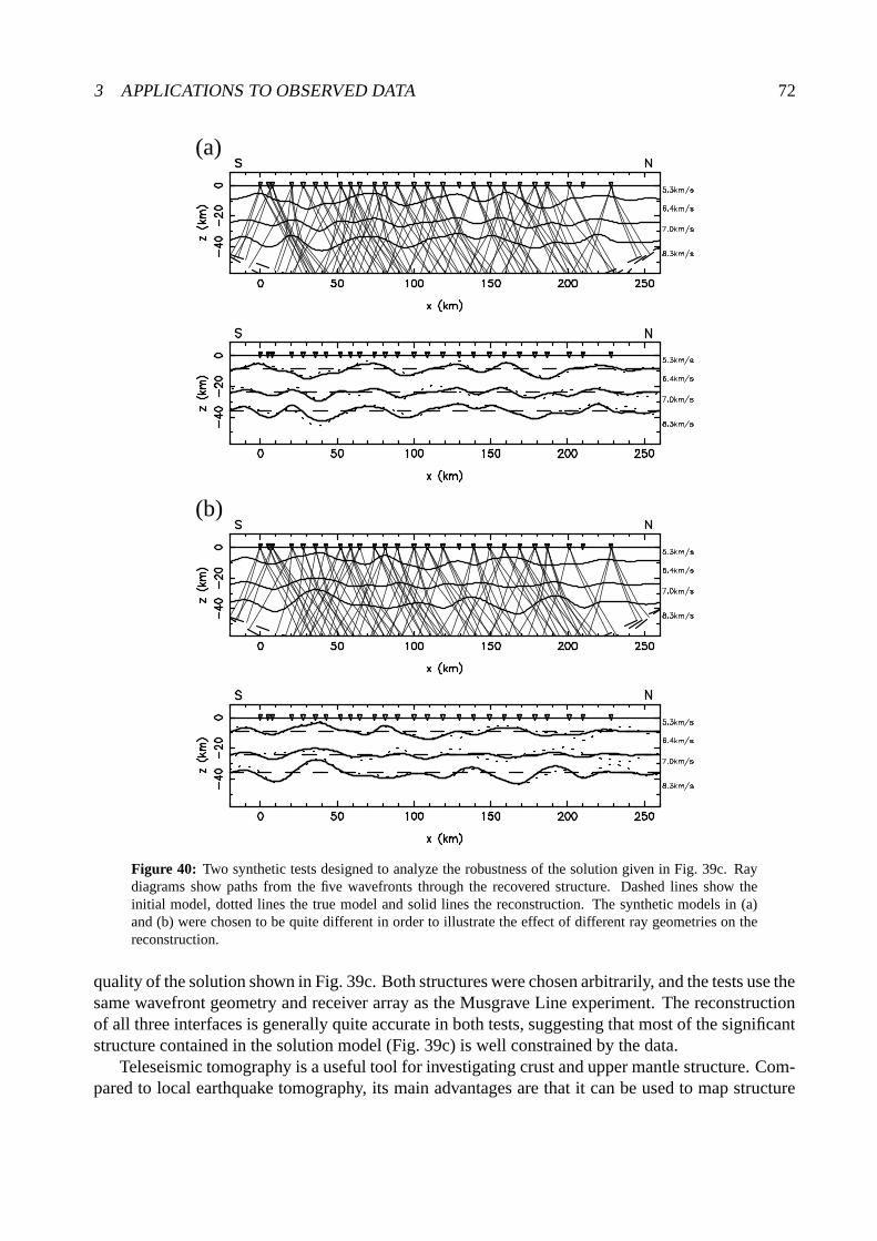
3 APPLICATIONS TO OBSERVED DATA 72
(b)
(a)
Figure 40: Two synthetic tests designed to analyze the robustness of the solution given in Fig. 39c. Raydiagrams show paths from the five wavefronts through the recovered structure. Dashed lines show theinitial model, dotted lines the true model and solid lines the reconstruction. The synthetic models in (a)and (b) were chosen to be quite different in order to illustrate the effect of different ray geometries on thereconstruction.
quality of the solution shown in Fig. 39c. Both structures were chosen arbitrarily, and the tests use thesame wavefront geometry and receiver array as the Musgrave Line experiment. The reconstructionof all three interfaces is generally quite accurate in both tests, suggesting that most of the significantstructure contained in the solution model (Fig. 39c) is well constrained by the data.
Teleseismic tomography is a useful tool for investigating crust and upper mantle structure. Com-pared to local earthquake tomography, its main advantages are that it can be used to map structure

4 FUTURE DEVELOPMENTS 73
at greater depths, and that it is not restricted to regions of active seismicity. However, the fact thatrelative traveltime residuals must be used means that only relative perturbations in lateral structurecan be resolved. In addition, the assumption that the model region is completely responsible forthe teleseismic traveltime residuals will not always be valid. Also, the near-vertical incidence angleof ray-paths and the sometimes poor azimuthal source coverage may lead to significant smearingeffects that in turn can lead to incorrect interpretations of results (see Keller et al., 2000). On theother hand, the interface structure shown in Fig. 39c demonstrates one advantage of the near-verticaltransmission of rays: highly complex lateral structure may be resolved. Wide-angle tomography (forexample) would have great difficulty imaging such structural complexity.
4 Future Developments
Traveltime tomography still remains the most popular approach for imaging subsurface structureon crustal and lithospheric scales. A wide array of schemes and algorithms can be found to tacklethese problems, and there is little doubt that traveltime tomography will continue to play a role inthe imaging of earth structure well into the future. Our aim here is to discuss, and to some degreespeculate on, the possible directions in which seismic traveltime tomography methods may develop,and whether it will continue to be the predominant interpretation technique for large datasets.
A current limitation of many traveltime tomography techniques is that they only consider first-arrivals and ignore the potentially vast amount of information contained in later arriving phases.Exceptions include coincident reflection tomography and wide-angle tomography. In the case ofreflection tomography, the number of phases picked usually corresponds to the number of interfacescontained in the model. Wide-angle tomography often includes later arriving reflection phases ina similar fashion. One of the principal difficulties in including traveltime information from later-arriving phases is that they are often obscured by the wavetrain of earlier arriving phases. This canmake identification difficult or impossible. Another difficulty is that even if coherent later arrivalscan be picked, they need to be related to model structure in order to be useful. For first-arrivalspicked from a seismogram, this is not required because we just need to search for the transmissionpaths through the structures that correspond to first arrivals. Of course, this task is not necessarilystraight forward, but the point is that we don’t need to know anything about the ray path a priori. Forwide-angle reflection phases, for example, we do need to know which interface they reflect from. Ifa layered parameterization is used, with the number of interfaces defined by the number of reflectionphases identified, then the problem of association may not arise. If the interfaces are defined a priori,then it may not be easy to relate later arrivals with structure. One approach is to constrain the initialmodel using only first-arrivals plus any other phases that can be confidently identified, and then usethe updated model to predict the traveltimes of other phases that weren’t picked but may be evidentin the data. A direct comparison with the observed data may allow additional phases to be pickedwith more confidence (Zelt, 1999). Multiples and phase conversions may also be identified in thismanner.
As well as the problems of detection and association of later arrivals described above, yet anotherdifficulty is that current methods of traveltime and ray path determination used in tomography areonly capable of finding a small subset of all possible arrivals. Obvious examples are the grid-basedmethods (Section 2.2.2) and SPR (Section 2.2.3), both of which are limited to first-arrivals. Bothmethods can be made to find reflection arrivals but not later arrivals associated with caustics. Tradi-tional ray tracing methods can find multiple arrivals - for example, by shooting an extremely dense

4 FUTURE DEVELOPMENTS 74
spread of rays, or by bending using a large variety of initial paths. However, in even moderatelycomplex media, these approaches would be very computationally expensive. Recently, significanteffort has been made in developing and implementing schemes for computing multivalued traveltimemaps. One approach, often referred to as wavefront construction, involves the discrete propagationof a wavefront through a medium by using local ray tracing from each wavefront surface. Raysare traced for a given time step, with the end points of the rays describing the geometry of the newwavefront. New rays are introduced by interpolation if diverging rays cause parts of the wavefrontto be poorly sampled. Multiple arrivals can be found using this scheme, including caustics. Thisbasic idea for locating multiple arrivals has been developed by a number of authors (e.g. Vinje et al.,1993; Ettrich & Gajewski, 1996; Lucio et al., 1996; Lambare et al., 1996; Vinje et al., 1996, 1999).Other schemes for finding multi-valued traveltime fields include Big Ray tracing (Benamou, 1996;Abgrall, 1999), which is a two-step procedure involving relatively coarse ray tracing followed by so-lution of the eikonal equation in spatial domains defined by adjacent ray paths, and Dynamic SurfaceExtension (Steinhoff et al., 2000), which shares similarities with wavefront construction.
The use of these schemes within a tomographic inversion may allow the traveltimes of more laterarrivals to be utilized, thus resulting in a potentially better constrained and more detailed solution.With the advent of modern high fidelity broad band digital seismometers, much more information onthe later arriving wavefield is being recorded, and new methodology such as wavefront constructionis required to better exploit this type of data.
Another area in which traveltime tomography may see more development is in the combining ofdifferent datasets in a simultaneous inversion. Usually, tomographic studies constrain structure us-ing just one type of data (reflection, wide-angle, local earthquake, teleseismic), but this need not bethe case provided more than one overlapping dataset is available. For example, wide-angle or LETarrays are likely to detect teleseismic arrivals during their deployment, which could be exploited to-gether with the principal dataset. Studies that combine different datasets have been carried out in thepast. Thurber (1983) and Ankeny et al. (1986) included refraction traveltimes from several explosivesources in a LET study, Parsons & Zoback (1997) simultaneously inverted local earthquake, explo-sive source and airgun traveltimes for the crustal structure of the San Francisco Peninsula, and Satoet al. (1996) simultaneously inverted local earthquake and teleseismic traveltime data to image struc-ture beneath the northeastern Japan arc. Methods that combine coincident reflection and wide-angledata in a simultaneous inversion have been developed by Wang & Braile (1996) and McCaughey &Singh (1997).
An often important component of subsurface velocity structure (especially in regions exhibitingsignificant deformation) that is frequently ignored in traveltime tomography studies is anisotropy.If the effects of anisotropy are severe enough, reconstructions that assume isotropy may produceerroneous results (Watanabe et al., 1996). The principal reason for ignoring anisotropy is that thedata can usually be satisfied adequately with an isotropic model. Introducing anisotropy effectivelyincreases the number of unknowns considerably for the same spatial resolution, meaning that theinverse problem is likely to become under-determined for most realistic datasets. As a consequence,traveltime tomography studies that have considered anisotropy usually make several assumptionsabout structure to reduce the number of unknowns. For example, Hearn (1996) inverted Pn trav-eltimes for lateral variations in both velocity and anisotropy in the uppermost mantle. The Mohosurface along which the ray paths propagate is assumed to be planar, and is parameterized in termsof cells. Each cell is associated with three unknowns: slowness and two coefficients of azimuthalanisotropy. Using multiple traveltime datasets and later arriving phases as suggested above may

4 FUTURE DEVELOPMENTS 75
make anisotropy tomography a more realistic proposition as data coverage will be greatly improved.The traveltimes of seismic phases constitute just one of the components of the recorded wave-
form. Combining traveltimes with amplitude information or using the shape of the waveform itselfis likely to yield much more information than traveltimes alone. Wang & Pratt (1997) combinedtraveltime and amplitude data in reflection tomography. They showed that using both datasets inan inversion for velocity or interface structure results in more accurate solutions compared to in-versions that invert only one data type. Neele et al. (1993) combined amplitude and traveltimesfrom a teleseismic dataset in a joint inversion for upper mantle structure. Pratt et al. (1996) demon-strated via 2-D synthetic tests that wavefield inversion of wide-angle seismic data produces velocitymodels of significantly greater resolution than traveltime inversion. Combining traveltime data withnon-seismic data is also likely to be further developed in the future. Using both gravity data andtraveltime data from wide-angle surveys to constrain crustal models has been done in the past. Forexample, Vogt et al. (1998) used a forward modeling approach to reconcile the two data types andproduce a structural model for the Hatton Basin and continental margin. Lees & VanDecar (1991)simultaneously inverted local earthquake traveltimes and Bouger gravity anomalies for crustal struc-ture in Western Washington.
Like most other areas of science, increases in computing power will also influence the way inwhich traveltime tomography will be approached in the future. Indeed, many of the potential futuredevelopments described above are reliant to some extent on the availability of greater computingpower. Computationally intensive methods for solving the inverse step of the problem like geneticalgorithms or simulated annealing (Section 2.3.3) will become more feasible for larger scale prob-lems. Currently, they are limited to perhaps several hundred unknowns at most. Also, the resultsfrom other studies could be used to improve model accuracy. For example, a teleseismic model couldbe embedded within a lower resolution global model to help prevent the mapping of aspherical man-tle structure into the local region of interest. This has been done in the context of regional-scaletraveltime inversion by Widiyantoro & van der Hilst (1997); in this study, global and regional travel-times were inverted simultaneously for a regional model on a 1◦ × 1◦ grid embedded within a globalmodel with a 5◦ × 5◦ cell size. However, the non-linearity of the problem was not accounted for inthe inversion, probably due in part to the significant computational expense involved.
In conclusion, there are still many new ways in which seismic traveltime information can be ex-ploited in tomographic-style problems. Most current methods use only a small subset of the recordedinformation, such as first arrivals. The new generation of methods are likely to be able to representcontinuous and discontinuous structure, use a wide variety of data geometries (e.g. coincident reflec-tion, wide-angle etc.), incorporate traveltimes from later phases, account for anisotropy, use otheraspects of the waveform such as amplitudes, and perhaps be able to use other data types such asgravity. The optimum method would use all the information contained in the recorded waveformto constrain structure, but practical implementation of such an approach is a long way off. Seismictraveltimes have played an important role in helping us to understand the structure and compositionof the crust and lithosphere via tomographic inversion, and will continue to do so well into the future.
ACKNOWLEDGMENTSWe thank Fiona Darbyshire for kindly supplying Fig. 29 and Fig. 30, and Frank Graeber for
kindly supplying Fig. 35, Fig. 36, Fig. 37 and Fig. 38. Greg Houseman is thanked for useful dis-cussions on an early version of this work, and an anonymous referee is thanked for constructivecomments on the original manuscript.

REFERENCES 76
References
Aarts, E. & Korst, J., 1989. Simulated Annealing and Boltzmann machines, John Wiley & Sons,Chichester.
Abers, G. A., 1994. Three-dimensional inversion of regional P and S arrival times in the EastAleutians and sources of subduction zone gravity highs, J. Geophys. Res., 99, 4395–4412.
Abgrall, R., 1999. Big ray-tracing and eikonal solver on unstructured grids: Application to thecomputation of a multivalued traveltime field in the Marmousi model, Geophysics, 64, 230–239.
Achauer, U., 1994. New ideas on the Kenya rift based on the inversion of the combined dataset ofthe 1985 and 1989/90 seismic tomography experiments, Tectonophysics, 236, 305–329.
Afnimar & Koketsu, K., 2000. Finite difference traveltime calculation for head waves travellingalong an irregular interface, Geophys. J. Int., 143, 729–734.
Aki, K. & Lee, W. H. K., 1976. Determination of the three-dimensional velocity anomalies under aseismic array using first P arrival times from local earthquakes 1. A homogeneous intial model,J. Geophys. Res., 81, 4381–4399.
Aki, K. & Richards, P. G., 1980. Quantitative seismology: theory and methods, W. H. Freeman, SanFrancisco.
Aki, K., Christoffersson, A., & Husebye, E. S., 1977. Determination of the three-dimensional seis-mic structure of the lithosphere, J. Geophys. Res., 82, 277–296.
Alkhalifah, T. & Fomel, S., 2001. Implementing the fast marching eikonal solver: Spherical versusCartesian coordinates, Geophysical Prospecting, 49, 165–178.
Ankeny, L. A., Braile, L. W., & Olsen, K. H., 1986. Upper crustal structure beneath the JemezMountains volcanic field, New Mexico, determined by three-dimensional simultaneous inversionof seismic refraction and earthquake data, J. Geophys. Res., 91, 6188–6198.
Asad, A. M., Pullammanappallil, S. K., Anooshehpoor, A., & Louie, J. N., 1999. Inversion of travel-time data for earthquake locations and three-dimensional velocity structure in the Eureka Valleyarea, eastern California, Bull. Seism. Soc. Am., 89, 796–810.
Bartels, R. H., Beatty, J. C., & Barsky, B. A., 1987. An introduction to splines for use in computergraphics and geometric modelling, Morgan Kaufmann, Los Altos.
Benamou, J. D., 1996. Big ray tracing: Multivalued travel time field computation using viscositysolutions of the Eikonal equation, J. Comp. Phys., 128, 463–474.
Benz, H. M. & Smith, R. B., 1984. Simultaneous inversion for lateral velocity variations andhypocenters in the Yellowstone region using earthquake and refraction data, J. Geophys. Res.,89, 1208–1220.
Benz, H. M., Zandt, G., & Oppenheimer, D. H., 1992. Lithospheric structure of northern Californiafrom teleseismic images of the upper mantle, J. Geophys. Res., 97, 4791–4807.
REFERENCES 77
Bijwaard, H. & Spakman, W., 2000. Non-linear global P-wave tomography by iterated linearizedinversion, Geophys. J. Int., 141, 71–82.
Bijwaard, H., Spakman, W., & Engdahl, E. R., 1998. Closing the gap between regional and globaltravel time tomography, J. Geophys. Res., 103, 30,055–30,078.
Bishop, T. P., Bube, K. P., Cutler, R. T., Langan, R. T., Love, P. L., Resnick, J. R., Shuey, R. T.,Spindler, D. A., & Wyld, H. W., 1985. Tomographic determination of velocity and depth inlaterally varying media, Geophysics, 50, 903–923.
Blundell, C. A., 1993. Resolution analysis of seismic P-wave velocity estimates using reflectiontomographic inversion, Ph.D. thesis, Monash University.
Bosch, M., 1997. P wave velocity tomography of the Venezuelan region from local arrival times, J.Geophys. Res., 102, 5455–5472.
Boschetti, F., Dentith, M. K., & List, R. D., 1996. Inversion of seismic refraction data using geneticalgorithms, Geophysics, 61, 1715–1727.
Cao, S. & Greenhalgh, S., 1994. Finite-difference solution of the eikonal equation using an efficient,first-arrival, wavefront tracking scheme, Geophysics, 59, 632–643.
Cara, M. & Leveque, J. J., 1987. Waveform inversion using secondary observables, Geophys. Res.Lett., 14, 1046–1049.
Carroll, S. & Beresford, G., 1996. Combining reflection tomography with layer replacement forvelocity analysis of near-surface reefs, Geophysics, 61, 561–569.
Cassell, B. R., 1982. A method for calculating synthetic seismograms in laterally varying media,Geophys. J. Royal Astr. Soc., 69, 339–354.
Cerveny, V., 1987. Ray tracing algorithms in three-dimensional laterally varying layered struc-tures, in Seismic tomography: With applications in global seismology and exploration geophysics,edited by G. Nolet, pp. 99–133, D. Reidel, Dordrecht.
Cerveny, V., 2001. Seismic Ray Theory, Cambridge University Press, Cambridge.
Cerveny, V. & Psencik, I., 1983. Gaussian beams and paraxial ray approximation in three-dimensional elastic inhomogeneous media, J. Geophys., 53, 1–15.
Cerveny, V., Klimes, L., & Psencik, I., 1984. Paraxial ray approximations in the computation ofseismic wavefields in inhomogeneous media, Geophys. J. Royal Astr. Soc., 79, 89–104.
Chapman, C. H. & Drummond, R., 1982. Body-wave seismograms in inhomogeneous media usingMaslov asymptotic theory, Bull. Seism. Soc. Am., 72, S277–S317.
Cheng, N. & House, L., 1996. Minimum traveltime calculations in 3-D graph theory, Geophysics,61, 1895–1898.
Chiarabba, C., Amoto, A., & Meghraoui, M., 1997. Tomographic images of the El Asnam faultzone, J. Geophys. Res., 102, 24,485–24,498.

REFERENCES 78
Chiu, S. K. L., Kanasewich, E. R., & Phadke, S., 1986. Three-dimensional determination of structureand velocity by seismic tomography, Geophysics, 51, 1559–1571.
Claerbout, J. F. & Muir, F., 1973. Robust modelling with erratic data, Geophysics, 38, 826–844.
Clowes, R. M., Zelt, C. A., Amor, J. R., & Ellis, R. M., 1995. Lithospheric structure in the southernCanadian Cordillera from a network of seismic refraction lines, Can. J. Earth Sci., 32, 1485–1513.
Constable, S. C., Parker, R. L., & Constable, C. G., 1987. Occam’s inversion: A practical algorithmfor generating smooth models from electromagnetic sounding data, Geophysics, 52, 289–300.
Creager, K. C. & Jordan, T. H., 1984. Slab penetration into the lower mantle, J. Geophys. Res., 89,3031–3049.
Darbyshire, F. A., Bjarnason, I. J., White, R. S., & Florenz, O. G., 1998. Crustal structure above theIceland mantle plume, imaged by the ICEMELT refraction profile, Geophys. J. Int., 135, 1131–1149.
Davis, P. M., 1991. Continental rift structures and dynamics with reference to teleseismic studies ofthe Rio Grande and East African rifts, Tectonophysics, 197, 309–325.
Day, A. J., Peirce, C., & Sinha, M. C., 2001. Three-dimensional crustal structure and magmachamber geometry at the intermediate-spreading, back-arc Valu Fa Ridge, Lau Basin - results ofa wide-angle seismic tomographic inversion, Geophys. J. Int., 146, 31–52.
Debayle, E. & Kennett, B. L. N., 2000. The australian continental upper mantle: Structure anddeformation inferred from surface waves, J. Geophys. Res., 105, 25,423–25,450.
Dijkstra, E. W., 1959. A note on two problems in connection with graphs, Numer. Math., 1, 269–271.
Dorbath, C. & Paul, A., 1996. Tomography of the Andean crust and mantle at 20◦S: First results ofthe Lithoscope experiment, Phys. Earth Planet. Inter., 97, 133–144.
Drijkoningen, G. G. & White, R. S., 1995. Seismic velocity structure of oceanic crust by inversionusing genetic algorithms, Geophys. J. Int., 123, 653–664.
Dueker, K., Humphreys, E., & Biasi, G., 1993. Teleseismic imaging of the western United Statesupper mantle structure using the simultaneous iterative reconstruction technique, in Seismic to-mography: theory and practice, edited by H. M. Iyer & K. Hirahara, pp. 265–298, Chapman &Hall, London.
Eberhart-Phillips, D., 1986. Three-dimensional velocity structure in northern California coast rangesfrom inversion of local earthquake arrival times, Bull. Seism. Soc. Am., 76, 1025–1052.
Eberhart-Phillips, D., 1990. Three-dimensional P and S velocity structure in the Coalinga Region,California, J. Geophys. Res., 95, 15,343–15,363.
Eberhart-Phillips, D. & Michael, A. J., 1993. Three-dimensional velocity structure, seismicity, andfault structure in the Parkfield Region, central California, J. Geophys. Res., 98, 15,737–15,758.
REFERENCES 79
Eberhart-Phillips, D. & Reyners, M., 1997. Continental subduction and three-dimensional crustalstructure: The northern South Island, New Zealand, J. Geophys. Res., 102, 11,848–11,861.
Ettrich, N. & Gajewski, D., 1996. Wave front construction in smooth media for prestack depthmigration, Pageoph, 148, 481–502.
Evans, J., Eberhart-Phillips, D., & Thurber, C., 1994. User’s manual for SI MU L P S12 for imagingvP and vP/vS: A derivative of the “Thurber” tomographic inversion SI MU L3 for local earth-quakes and explosions, Open file report 431, U.S. Geological Survey.
Evans, J. R., 1982. Compressional wave velocity structure of the upper 350 km under the EasternSnake River Plain near Rexburg, Idaho, J. Geophys. Res., 87, 2654–2670.
Faria, E. L. & Stoffa, P. L., 1994. Traveltime computation in transversely isotropic media, Geo-physics, 59, 272–281.
Farra, V. & Madariaga, R., 1988. Non-linear reflection tomography, Geophys. J., 95, 135–147.
Fischer, R. & Lees, J. M., 1993. Shortest path ray tracing with sparse graphs, Geophysics, 58,987–996.
Fletcher, R. & Reeves, C. M., 1964. Function minimization by conjugate gradients, Comput. J., 7,149–154.
Frederiksen, A. W., Bostock, M. G., VanDecar, J. C., & Cassidy, J. F., 1998. Seismic structure ofthe upper mantle beneath the northern Canadian Cordillera from teleseismic travel-time inversion,Tectonophysics, 294, 43–55.
Gjøystdal, H., Reinhardsen, J. E., & Ursin, B., 1984. Traveltime and wavefront curvature calcula-tions in three-dimensional inhomogeneous layered media with curved interfaces, Geophysics, 49,1466–1494.
Glahn, A. & Granet, M., 1993. Southern Rhine Graben: Small-wavelength tomographic study andimplications for the dynamic evolution of the graben, Geophys. J. Int., 113, 399–418.
Goldberg, D. E., 1989. Genetic Algorithms in Search, Optimization, and Machine Learning,Addison-Wesley, Reading.
Gorbatov, A., Widiyantoro, S., Fukao, Y., & Gordeev, E., 2000. Signature of remnant slabs in theNorth Pacific from P-wave tomography, Geophys. J. Int., 142, 27–36.
Gorbatov, A., Fukao, Y., Widiyantoro, S., & Gordeev, E., 2001. Seismic evidence for a mantle plumeoceanwards of the Kamchatka-Aleutian trench junction, Geophys. J. Int., 146, 282–288.
Grad, M., Shiobara, H., Janik, T., Guterch, A., & Shimamura, H., 1997. Crustal model of theBransfield Rift, West Antarctica, from detailed OBS refraction experiments, Geophys. J. Int.,130, 506–518.
Graeber, F. M. & Asch, G., 1999. Three-dimensional models of P wave velocity and P-to-S velocityratio in the southern central Andes by simultaneous inversion of local earthquake data, J. Geophys.Res., 104, 20,237–20,256.

REFERENCES 80
Graeber, F. M., Houseman, G. A., & Greenhalgh, S. A., 2002. Regional teleseismic tomography ofthe western Lachlan Orogen and the Newer Volcanic Province, southeast Australia, Geophys. J.Int., 149, 249–266.
Granet, M. & Trampert, J., 1989. Large-scale P-velocity structures in the Euro-Mediterranean area,Geophys. J. Int., 99, 583–594.
Grevemeyer, I., Fleuh, E. R., Reichert, C., Biala, J., Klaschen, D., & Kopp, C., 2001. Crustalarchitecture and deep structure of the Ninetyeast Ridge hotspot trail from active-source oceanbottom seismology, Geophys. J. Int., 144, 414–431.
Gubbins, D., 1992. Seismology and plate tectonics, Cambridge University Press, Cambridge.
Guiziou, J. L., Mallet, J. L., & Madariaga, R., 1996. 3-D seismic reflection tomography on top ofthe GOCAD depth modeler, Geophysics, 61, 1499–1510.
Gurbuz, C. & Evans, J. R., 1991. A seismic refraction study of the western Tuz Golu basin, centralTurkey, Geophys. J. Int., 106, 239–251.
Hammer, P. T. C., Dorman, L. M., Hildebrand, J. A., & Cornuelle, B. D., 1994. Jasper Seamountstructure: Seafloor seismic refraction tomography, J. Geophys. Res., 99, 6731–6752.
Hasegawa, A., Umino, N., & Takagi, A., 1978. Double-planed deep seismic zone and upper-mantlestructure in the northeastern Japan arc, Geophys. J. Royal Astr. Soc., 54, 281–296.
Haslinger, F., Kissling, E., Ansorge, J., Hatzfeld, D., Papadimitriou, E., Karakostas, V., Makropou-los, K., Kahle, H. G., & Peter, Y., 1999. 3D crustal structure from local earthquake tomographyaround the Gulf of Arta (Ionian region, NW Greece), Tectonophysics, 304, 201–218.
Hearn, T. M., 1996. Anisotropic Pn tomography in the western United States, J. Geophys. Res.,101, 8403–8414.
Hestenes, M. & Stiefel, E., 1952. Methods of conjugate gradients for solving linear systems, Nat.Bur. Stand. J. Res., 49, 409–436.
Hildebrand, J. A., Dorman, L. M., Hammer, P. T. C., Schreiner, A. E., & Cornuelle, B. D., 1989.Seismic tomography of Jasper Seamount, Geophys. Res. Lett., 16, 1355–1358.
Hole, J. A., 1992. Nonlinear high-resolution three-dimensional travel-time tomography, J. Geophys.Res., 97, 6553–6562.
Hole, J. A. & Zelt, B. C., 1995. 3-D finite-difference reflection travel times, Geophys. J. Int., 121,427–434.
Hole, J. A., Clowes, R. M., & Ellis, R. M., 1992. Interface inversion using broadside seismicrefraction data and three-dimensional traveltime calculations, J. Geophys. Res., 97, 3417–3429.
Humphreys, E. & Clayton, R. W., 1988. Adaption of back projection tomography to seismic traveltime problems, J. Geophys. Res., 93, 1073–1085.

REFERENCES 81
Humphreys, E. D. & Clayton, R. W., 1990. Tomographic image of the Southern California Mantle,J. Geophys. Res., 95, 19,725–19,746.
Inoue, H., Fukao, Y., Tanabe, K., & Ogata, Y., 1990. Whole mantle P-wave travel time tomography,Phys. Earth Planet. Inter., 59, 294–328.
Iwasaki, T., Hirata, N., Kanazawa, T., Melles, J., Suyehiro, K., Urabe, T., Moller, L., Makris, J., &Shimamura, H., 1990. Crustal and upper mantle structure in the Ryukyu Island Arc deduced fromdeep seismic sounding, Geophys. J. Int., 102, 631–651.
Iwasaki, T., Ozel, O., Moriya, T., Sakai, S., Suzuki, S., Aoki, G., Maeda, T., & Iidaka, T., 1998.Lateral structural variations across a collision zone in central Hokkaido, Japan, as revealed bywide-angle seismic experiments, Geophys. J. Int., 132, 435–457.
Iyer, H. & Hirahara, K., 1993. Seismic Tomography: Theory and Practice, Chapman & Hall, Lon-don.
Jarchow, C. M., Catchings, R. D., & Lutter, W. J., 1994. Large-explosive source, wide-recordingaperture, seismic profiling on the Columbia Plateau, Washington, Geophysics, 59, 259–271.
Julian, B. R. & Gubbins, D., 1977. Three-dimensional seismic ray tracing, J. Geophys., 43, 95–113.
Kanasewich, E., Burianyk, M. J. A., Ellis, R. M., Clowes, R. M., White, D. J., Lote, T., Forsyth,D. A., Luetgert, J. A., & Spence, G. D., 1994. Crustal velocity structure of the Omineca Belt,southwestern Canadian Cordillera, J. Geophys. Res., 99, 2653–2670.
Kanasewich, E. R. & Chiu, S. K. L., 1985. Least-squares inversion of spatial seismic refraction data,Bull. Seism. Soc. Am., 75, 865–880.
Kao, H. & Rau, R. J., 1999. Detailed structures of the subducted Philippine Sea plate beneathnortheast Taiwan: A new type of double seismic zone, J. Geophys. Res., 104, 1015–1033.
Kawakatsu, H., 1985. Double seismic zone in Tonga, Nature, 316, 53–55.
Keller, W. R., Anderson, D. L., & Clayton, R. W., 2000. Resolution of tomographic models of themantle beneath Iceland, Geophys. Res. Lett., 27, 3993–3996.
Kennett, B. L. N., 1998. Seismic wave propagation and seismic tomography, Research School ofEarth Sciences, Institute of Advanced Studies, The Australian National University, Canberra.
Kennett, B. L. N., 2002. The Seismic Wavefield, Volume 2: Interpretation of Seismograms on Re-gional and Global Scales, Cambridge University Press, Cambridge.
Kennett, B. L. N. & Engdahl, E. R., 1991. Traveltimes for global earthquake location and phaseidentification, Geophys. J. Int., 105, 429–465.
Kennett, B. L. N., Sambridge, M. S., & Williamson, P. R., 1988. Subspace methods for large scaleinverse problems involving multiple parameter classes, Geophys. J., 94, 237–247.
Kim, S., 2001. An O(N ) level set method for eikonal equations, SIAM J. Sci. Comput., 22, 2178–2193.

REFERENCES 82
Kirkpatrick, S., Gelatt, Jr, C. D., & Vecchi, M. P., 1983. Optimization by simulated annealing,Science, 220, 671–680.
Klimes, L. & Kvasnicka, M., 1994. 3-D network ray tracing, Geophys. J. Int., 116, 726–738.
Kodaira, S., Mjelde, R., Gunnarsson, K., Shiobara, H., & Shimamura, H., 1998. Structure of the JanMayen microcontinent amd implications for its evolution, Geophys. J. Int., 132, 383–400.
Kohler, M. D., 1997. Three-dimensional velocity structure and resolution of the core-mantle bound-ary region from whole-mantle inversions of body waves, Phys. Earth Planet. Inter., 101, 85–104.
Kohler, M. D. & Davis, P. M., 1997. Crustal thickness variations in southern California from LosAngeles Region Seismic Experiment passive phase teleseismic travel times, Bull. Seism. Soc. Am.,87, 1330–1344.
Korenaga, J., Holbrook, W. S., Kent, G. M., Kelemen, R. S., Detrick, R. S., Larsen, H. C., Hopper,J. R., & Dahl-Jensen, T., 2000. Crustal structure of the southeast Greenland margin from jointrefraction and reflection tomography, J. Geophys. Res., 105, 21,591–21,614.
Kosloff, D., Sherwood, J., Koren, Z., Machet, E., & Falkovitz, Y., 1996. Velocity and interface depthdetermination by tomography of depth migrated gathers, Geophysics, 61, 1511–1523.
Kreyszig, E., 1993. Advanced engineering mathematics, John Wiley & Sons, Inc., New York.
Lambare, G., Lucio, P. S., & Hanyga, A., 1996. Two-dimensional multivalued traveltime and ampli-tude maps by uniform sampling of a ray field, Geophys. J. Int., 125, 584–598.
Lambeck, K. & Burgess, G., 1992. Deep crustal structure of the Musgrave Block, central Australia:results from teleseismic traveltime anomalies, Australian Journal of Earth Sciences, 39, 1–19.
Lambeck, K., Burgess, G., & Shaw, R. D., 1988. Teleseismic travel-time anomalies and deep crustalstructure in central Australia, Geophys. J., 94, 105–124.
Langan, R. T., Lerche, I., & Cutler, R. T., 1985. Tracing of rays through heterogeneous media: Anaccurate and efficient procedure, Geophysics, 50, 1456–1465.
Lee, W. H. K. & Pereyra, V., 1993. Mathematical introduction to seismic tomography, in Seismictomography: theory and practice, edited by H. M. Iyer & K. Hirahara, pp. 9–22, Chapman &Hall, London.
Lees, J. M. & VanDecar, J. C., 1991. Seismic tomography constrained by Bouguer gravity anomalies:Applications in western Washington, Pageoph, 135, 31–52.
Leveque, J. J. & Masson, F., 1999. From ACH tomographic models to absolute velocity models,Geophys. J. Int., 137, 621–629.
Leveque, J. J., Rivern, L., & Wittlinger, G., 1993. On the use of the checker-board test to assess theresolution of tomographic inversions, Geophys. J. Int., 115, 313–318.
Lizarralde, D. & Holbrook, W. S., 1997. U.S. mid-Atlantic margin structure and early thermalevolution, J. Geophys. Res., 102, 22,855–22,875.

REFERENCES 83
Louden, K. E. & Fan, J., 1998. Crustal structures of Grenville, Makkovik, and southern Nainprovinces along the Lithoprobe ECSOOT Transect: Regional seismic refraction and gravity mod-els and their tectonic implications, Can. J. Earth Sci., 35, 583–601.
Luca, G. D., Filippi, L., Caccamo, D., Neri, G., & Scarpa, R., 1997. Crustal structure and seismicityof southern Tyrrhenian basin, Phys. Earth Planet. Inter., 103, 117–133.
Lucio, P. S., Lambare, G., & Hanyga, A., 1996. 3D multivalued travel time and amplitude maps,Pageoph, 148, 449–479.
Lutter, W. J. & Nowack, R. L., 1990. Inversion for crustal structure using reflections from thePASSCAL Ouachita experiment, J. Geophys. Res., 95, 4633–4646.
Lutter, W. J., Nowack, R. L., & Braile, L., 1990. Seismic imaging of upper crustal structure usingtravel times from the PASSCAL Ouachita experiment, J. Geophys. Res., 95, 4621–4631.
Lutter, W. J., Catchings, R. D., & Jarchow, C. M., 1994. An image of the Columbia Plateau frominversion of high-resolution seismic data, Geophysics, 59, 1278–1289.
McCaughey, M. & Singh, S. C., 1997. Simultaneous velocity and interface tomography of normal-incidence and wide-aperture seismic traveltime data, Geophys. J. Int., 131, 87–99.
McMechan, G. A., 1983. Seismic tomography in boreholes, Geophys. J. Royal Astr. Soc., 74, 601–612.
McQueen, H. W. S. & Lambeck, K., 1996. Determination of crustal structure in central Australia byinversion of traveltime residuals, Geophys. J. Int., 126, 645–662.
Menke, W., 1989. Geophysical data analysis: Discrete inverse theory, Academic Press, New York.
Mjelde, R., Digranes, P., Shimamura, H., Shiobara, H., Kodaira, S., Brekke, H., Egebjerg, T.,Sørenes, N., & Thorbjørnsen, S., 1998. Crustal structure of the northern part of the Vøring Basin,mid-Norway margin, from wide-angle seismic and gravity data, Tectonophysics, 293, 175–205.
Morgan, R. P. L., Barton, P. J., Warner, M., Morgan, J., Price, C., & Jones, K., 2000. Lithosphericstructure north of Scotland - I. P-wave modelling, deep reflection profiles and gravity, Geophys.J. Int., 142, 716–736.
Morozov, I. B., Smithson, S. B., Hollister, L. S., & Diebold, J. B., 1998. Wide-angle seismic imagingacross accreted terranes, southeastern Alaska and western British Columbia, Tectonophysics, 299,281–296.
Mosegaard, K. & Sambridge, M., 2002. Monte Carlo analysis of inverse problems, Inverse Problems,18, R29–R54.
Moser, T. J., 1991. Shortest path calculation of seismic rays, Geophysics, 56, 59–67.
Nakanishi, I., 1985. Three-dimensional structure beneath the Hokkaido-Tohoku region as derivedfrom a tomographic inversion of P-arrival times, J. Phys. Earth, 33, 241–256.

REFERENCES 84
Nakanishi, I. & Yamaguchi, K., 1986. A numerical experiment on nonlinear image reconstructionfrom first-arrival times for two-dimensional island arc structure, J. Phys. Earth, 34, 195–201.
Navin, D. A., Peirce, C., & Sinha, M. C., 1998. The RAMESSES experiment -II. Evidence foraccumulated melt beneath a slow spreading ridge from wide-angle refraction and multichannelreflection seismic profiles, Geophys. J. Int., 135, 746–772.
Neele, F., VanDecar, J., & Snieder, R., 1993. The use of P wave amplitude data in a joint inversionwith travel times for upper mantle velocity structure, J. Geophys. Res., 98, 12,033–12,054.
Nielsen, L., Thybo, H., & Solodilov, L., 1999. Seismic tomographic inversion of Russian PNE dataalong profile Kraton, Geophys. Res. Lett., 26, 3413–3416.
Nolet, G., 1985. Solving or resolving inadequate and noisy tomographic systems, J. Comp. Phys.,61, 463–482.
Nolet, G., 1987. Waveform tomography, in Seismic tomography: With applications in global seis-mology and exploration geophysics, edited by G. Nolet, pp. 301–322, D. Reidel, Dordrecht.
Nolet, G., 1987. Seismic tomography: With applications in global seismology and explorationgeophysics, D. Reidel, Dordrecht.
Nolet, G., 1990. Partitioned waveform inversion and two-dimensional structure under the networkof autonomously recording seismographs, J. Geophys. Res., 95, 8499–8512.
Nowack, R. L. & Lyslo, J. A., 1989. Frechet derivatives for curved interfaces in the ray approxima-tion, Geophys. J., 97, 497–509.
Oncescu, M. C., Burlacu, V., Anghel, M., & Smalbergher, V., 1984. Three-dimensional P-wavevelocity image under the Carpathian Arc, Tectonophysics, 106, 305–319.
Papazachos, C. & Nolet, G., 1997. P and S deep velocity structure of the Hellenic area obtained byrobust nonlinear inversion of travel times, J. Geophys. Res., 102, 8349–8367.
Parker, R. L., 1994. Geophysical inverse theory, Princeton University Press, Princeton.
Parsons, T. & Zoback, M. L., 1997. Three-dimensional upper crustal velocity structure beneath SanFrancisco Peninsula, California, J. Geophys. Res., 102, 5473–5490.
Parsons, T., McCarthy, J., Kohler, W. M., Ammon, C. J., Benz, H. M., Hole, J. A., & Criley, E. E.,1996. Crustal structure of the Colorada Plateau, Arizona: Application of new long-offset seismicdata analysis techniques, J. Geophys. Res., 101, 11,173–11,194.
Pereyra, V., Lee, W. H. K., & Keller, H. B., 1980. Solving two-point seismic-ray tracing problemsin a heterogeneous medium, Bull. Seism. Soc. Am., 70, 79–99.
Podvin, P. & Lecomte, I., 1991. Finite difference computation of traveltimes in very contrastedvelocity models: a massively parallel approach and its associated tools, Geophys. J. Int., 105,271–284.

REFERENCES 85
Popovici, A. M. & Sethian, J. A., 2002. 3-D imaging using higher order fast marching traveltimes,Geophysics, 67, 604–609.
Pratt, R. G., Song, Z. M., Williamson, P., & Warner, M., 1996. Two-dimensional velocity modelsfrom wide-angle seismic data by wavefield inversion, Geophys. J. Int., 124, 323–340.
Press, W. H., Tuekolsky, S. A., Vetterling, W. T., & Flannery, B. P., 1992. Numerical Recipes inFORTRAN, Cambridge University Press, Cambridge.
Priestley, K., Cipar, J., Egorkin, A., & Pavlenkova, N., 1994. Upper-mantle velocity structure be-neath the Siberian platform, Geophys. J. Int., 118, 369–378.
Prothero, W. A., Taylor, W. J., & Eickemeyer, J. A., 1988. A fast, two-point, three-dimensionalraytracing algorithm using a simple step search method, Bull. Seism. Soc. Am., 78, 1190–1198.
Protti, M., Schwartz, S. Y., & Zandt, G., 1996. Simultaneous inversion for earthquake location andvelocity structure beneath central Costa Rica, Bull. Seism. Soc. Am., 86, 19–31.
Pullammanappallil, S. K. & Louie, J. N., 1993. Inversion of seismic reflection traveltimes using anonlinear optimization scheme, Geophysics, 58, 1607–1620.
Qin, F., Luo, Y., Olsen, K. B., Cai, W., & Schuster, G. T., 1992. Finite-difference solution of theeikonal equation along expanding wavefronts, Geophysics, 57, 478–487.
Rawlinson, N., 2000. Inversion of Seismic Data for Layered Crustal Structure, Ph.D. thesis, MonashUniversity.
Rawlinson, N. & Houseman, G. A., 1998. Inversion for interface structure using teleseismic travel-time residuals, Geophys. J. Int., 133, 756–772.
Rawlinson, N., Houseman, G. A., & Collins, C. D. N., 2001a. Inversion of seismic refraction andwide-angle reflection traveltimes for 3-D layered crustal structure, Geophys. J. Int., 145, 381–401.
Rawlinson, N., Houseman, G. A., Collins, C. D. N., & Drummond, B. J., 2001b. New evidence ofTasmania’s tectonic history from a novel seismic experiment, Geophys. Res. Lett., 28, 3337–3340.
Recq, M., Goslin, J., Charvis, P., & Operto, S., 1998. Small-scale crustal variability within anintraplate structure: The Crozet Bank (southern Indian Ocean), Geophys. J. Int., 134, 145–156.
Riahi, M. A. & Juhlin, C., 1994. 3-D interpretation of reflected arrival times by finite-differencetechniques, Geophysics, 59, 844–849.
Riahi, M. A. & Lund, C. E., 1994. Two-dimensional modelling and interpretation of seismic wide-angle data from the western Gulf of Bothnia, Tectonophysics, 239, 149–164.
Riahi, M. A., Lund, C. E., & Pederson, L. B., 1997. Three-dimensional image of the Moho undula-tions beneath the Gulf of Bothnia using wide-angle seismic data, Geophys. J. Int., 129, 461–471.
Ritsema, J., Nyblade, A. A., Owens, T. J., Langston, C. A., & VanDecar, J. C., 1998. Upper mantleseismic velocity structure beneath Tanzania, east Africa: Implications for the stability of cratoniclithosphere, J. Geophys. Res., 103, 21,201–21,213.
REFERENCES 86
Ryberg, T., Wenzel, F., Mechie, J., Egorkin, A., Fuchs, K., & Solodilov, L., 1996. Two-dimensionalvelocity structure beneath northern Eurasia derived from the super long-range seismic profileQuartz, Bull. Seism. Soc. Am., 86, 857–867.
Saltzer, R. L. & Humphreys, E. D., 1997. Upper mantle P wave velocity structure of the easternSnake River Plain and its relationship to geodynamic models of the region, J. Geophys. Res., 102,11,829–11,841.
Sambridge, M. & Mosegaard, K., 2001. Monte Carlo methods in geophysical inverse problems, Rev.of Geophys., submitted.
Sambridge, M. S., 1990. Non-linear arrival time inversion: Constraining velocity anomalies byseeking smooth models in 3-D, Geophys. J. Int., 102, 653–677.
Sambridge, M. S. & Drijkoningen, G., 1992. Genetic algorithms in seismic waveform inversion,Geophys. J. Int., 109, 323–342.
Sambridge, M. S. & Kennett, B. L. N., 1990. Boundary value ray tracing in a heterogeneous medium:A simple and versatile algorithm, Geophys. J. Int., 101, 157–168.
Sato, T., Kosuga, M., & Tanaka, K., 1996. Tomographic inversion for P wave velocity structurebeneath the northeastern Japan arc using local and teleseismic data, J. Geophys. Res., 101, 17,597–17,615.
Scales, J. A., 1987. Tomographic inversion via the conjugate gradient method, Geophysics, 52,179–185.
Scales, J. A. & Snieder, R., 1997. To Bayes or not to Bayes, Geophysics, 62, 1045–1046.
Scott, J. S., Masters, T. G., & Vernon, F. L., 1994. 3-D velocity structure of the San Jacinto faultzone near Anza, California-I. P waves, Geophys. J. Int., 119, 611–626.
Seber, D., Barazangi, M., Tadili, B. A., Ramdani, M., Ibenbrahim, A., & Sari, D. B., 1996. Three-dimensional upper mantle structure beneath the intraplate Atlas and interplate Rif mountains ofMorocco, J. Geophys. Res., 101, 3125–3138.
Sethian, J. A., 1999. Level Set Methods and Fast marching Methods, Cambridge University Press,Cambridge.
Sethian, J. A. & Popovici, A. M., 1999. 3-D traveltime computation using the fast marching method,Geophysics, 64, 516–523.
Shalev, E., 1993. Cubic B-slines: Strategies of translating a simple structure to B-spline parameter-ization, Bull. Seism. Soc. Am., 83, 1617–1627.
Shaw, P. R. & Orcutt, A., 1985. Waveform inversion of seismic refraction data and applications toyoung Pacific crust, Geophys. J. Royal Astr. Soc., 82, 375–414.
Smith, W. H. F. & Wessel, P., 1990. Gridding with continuous curvature splines in tension, Geo-physics, 55, 293–305.

REFERENCES 87
Snieder, R., 1998. The role of nonlinearity in inverse problems, Inverse Problems, 14, 387–404.
Snieder, R. & Sambridge, M., 1993. The ambiguity in ray perturbation theory, J. Geophys. Res., 98,22,021–22,034.
Spakman, W., 1991. Delay-time tomography of the upper mantle below Europe, the Mediterraneanand Asia Minor, Geophys. J. Int., 107, 309–332.
Spakman, W., 1993. Iterative strategies for nonlinear travel-time tomography using global earth-quake data, in Seismic tomography: theory and practice, edited by H. M. Iyer & K. Hirahara, pp.190–226, Chapman & Hall, London.
Staples, R. K., White, R. S., Brandsdottir, Menke, W., Maguire, P. K. H., & McBride, J. H., 1997.Faroe-Iceland Ridge experiment 1. Crustal structure of northeastern Iceland, J. Geophys. Res.,102, 7849–7866.
Steck, L. K., Thurber, C. H., Fehler, M., Lutter, W. J., Roberts, P. M., Baldridge, W. S., Stafford,D. G., & Sessions, R., 1998. Crust and upper mantle P wave velocity structure beneath Vallescaldera, New Mexico: Results from the Jemez teleseismic tomography experiment, J. Geophys.Res., 103, 24,301–24,320.
Steinhoff, J., Fan, M., & Wang, L., 2000. A new Eulerian method for the computation of propagatingshort acoustic and electromagnetic pulses, J. Comp. Phys., 157, 683–706.
Tarantola, A., 1987. Inverse problem theory, Elsevier, Amsterdam.
Telford, W. M., Geldart, L. P., Sheriff, R. E., & Keys, D. A., 1976. Applied Geophysics, CambridgeUniversity Press, Cambridge.
Telford, W. M., Geldart, L. P., & Sheriff, R. E., 1990. Applied Geophysics, Cambridge UniversityPress, Cambridge.
Thomson, C. J. & Gubbins, D., 1982. Three-dimensional lithospheric modelling at NORSAR: lin-earity of the method and amplitude variations from the anomalies, Geophys. J. Royal Astr. Soc.,71, 1–36.
Thurber, C. H., 1983. Earthquake locations and three-dimensional crustal structure in the CoyoteLake area, central California, J. Geophys. Res., 88, 8226–8236.
Thurber, C. H., 1993. Local earthquake tomography: Velocities and Vp/Vs - theory, in Seismictomography: theory and practice, edited by H. M. Iyer & K. Hirahara, pp. 563–583, Chapman &Hall, London.
Thurber, C. H. & Ellsworth, W. L., 1980. Rapid solution of ray tracing problems in heterogeneousmedia, Bull. Seism. Soc. Am., 70, 1137–1148.
Toomey, D. R., Solomon, S. C., & Purdy, G. M., 1994. Tomographic imaging of the shallow crustalstructure of the East Pacific Rise at 9◦30′N, J. Geophys. Res., 99, 24,135–24,157.
Um, J. & Thurber, C., 1987. A fast algorithm for two-point seismic ray tracing, Bull. Seism. Soc.Am., 77, 972–986.
REFERENCES 88
van der Hilst, R. D., Widiyantoro, S., & Engdahl, E. R., 1997. Evidence for deep mantle circulationfrom global tomography, Nature, 386, 578–584.
van Trier, J. & Symes, W. W., 1991. Upwind finite-difference calculation of traveltimes, Geophysics,56, 812–821.
VanDecar, J. C., 1991. Upper-mantle structure of the Cascadia subduction zone from non-linearteleseismic travel-time inversion, Ph.D. thesis, University of Washington.
VanDecar, J. C. & Snieder, R., 1994. Obtaining smooth solutions to large, linear, inverse problems,Geophysics, 59, 818–829.
VanDecar, J. C., James, D. E., & Assumpcao, M., 1995. Seismic evidence for a fossil mantle plumebeneath South America and implications for plate driving forces, Nature, 378, 25–31.
Vidale, J. E., 1988. Finite-difference calculations of traveltimes, Bull. Seism. Soc. Am., 78, 2062–2076.
Vidale, J. E., 1990. Finite-difference calculations of traveltimes in three dimensions, Geophysics,55, 521–526.
Vinje, V., Iversen, E., & Gjøystdal, H., 1993. Traveltime and amplitude estimation using wavefrontconstruction, Geophysics, 58, 1157–1166.
Vinje, V., Iversen, E., Astebøl, K., & Gjøystdal, H., 1996. Estimation of multivalued arrivals in 3Dmodels using wavefront construction - Part I, Geophysical Prospecting, 44, 819–842.
Vinje, V., Astebøl, K., Iversen, E., & Gjøystdal, H., 1999. 3-D ray modelling by wavefront construc-tion in open models, Geophysical Prospecting, 64, 1912–1919.
Vogt, U., Makris, J., O’Reilly, B., Hausser, F., Readman, P. W., Jacob, A. W. B., & Shannon, P. M.,1998. The Hatton Basin and continental margin: Crustal structure from wide-angle seismic andgravity data, J. Geophys. Res., 103, 12,545–12,566.
Walck, M. C., 1988. Three-dimensional Vp/Vs variations for the Coso region, California, J. Geo-phys. Res., 93, 2047–2052.
Walck, M. C. & Clayton, R. W., 1987. P wave velocity variations in the Coso region, California,derived from local earthquake travel times, J. Geophys. Res., 92, 393–405.
Wang, B. & Braile, L. W., 1996. Simultaneous inversion of reflection and refraction seismic dataand application to field data from the northern Rio Grande rift, Geophys. J. Int., 125, 443–458.
Wang, W. & Houseman, G. A., 1994. Inversion of reflection seismic amplitude data for interfacegeometry, Geophys. J. Int., 117, 92–110.
Wang, Y. & Houseman, G. A., 1995. Tomographic inversion of reflection seismic amplitude data forvelocity variation, Geophys. J. Int., 123, 355–372.
Wang, Y. & Pratt, R. G., 1997. Sensitivities of seismic traveltimes and amplitudes in reflectiontomography, Geophys. J. Int., 131, 618–642.

REFERENCES 89
Watanabe, T., Hirai, t., & Sassa, K., 1996. Seismic traveltime tomography in anisotropic heteroge-neous media, J. Appl. Geophys., 35, 133–143.
Weiland, C. M., Steck, L. K., Dawson, P. B., & Korneev, V. A., 1995. Nonlinear teleseismic to-mography at Long Valley caldera, using three-dimensional minimum travel time ray tracing, J.Geophys. Res., 100, 20,379–20,390.
White, D. J., 1989. Two-dimensional seismic refraction tomography, Geophys. J., 97, 223–245.
Whitley, D. L., 1994. A genetic algorithm tutorial, Stats. and Comput., 4, 65–85.
Widiyantoro, S. & van der Hilst, R., 1997. Mantle structure beneath Indonesia inferred from high-resolution tomographic imaging, Geophys. J. Int., 130, 167–182.
Wiggins, S. M., Dorman, L. M., Cornuelle, B. D., & Hildebrand, J. A., 1996. Hess deep rift valleystructure from seismic tomography, J. Geophys. Res., 101, 22,335–22,353.
Williamson, P. R., 1990. Tomographic inversion in reflection seismology, Geophys. J. Int., 100,255–274.
Ye, S., Flueh, E. R., Klaeschen, D., & von Huene, R., 1997. Crustal structure along the EDGEtransect beneath the Kodiak shelf off Alaska derived from OBH seismic refraction data, Geophys.J. Int., 130, 283–302.
Yilmaz, O., 1987. Seismic data processing, Society of Exploration Geophysicists, Tulsa.
Zelt, B. C., Ellis, R. M., Clowes, R. M., & Hole, J. A., 1996. Inversion of three-dimensional wide-angle seimic data from the southwestern Canadia Cordillera, J. Geophys. Res., 286, 209–221.
Zelt, B. C., Ellis, R. M., Zelt, C. A., Hyndman, R. D., Lowe, C., Spence, G. D., & Fisher,M. A., 2001. Three-dimensional crustal velocity structure beneath the Strait of Georgia, BritishColumbia, Geophys. J. Int., 144, 695–712.
Zelt, C. A., 1998. Lateral velocity resolution from three-dimensional seismic refraction data, Geo-phys. J. Int., 135, 1101–1112.
Zelt, C. A., 1999. Modelling strategies and model assessment for wide-angle seismic traveltimedata, Geophys. J. Int., 139, 183–204.
Zelt, C. A. & Barton, P. J., 1998. Three-dimensional seismic refraction tomography: A comparisonof two methods applied to data from the Faeroe Basin, J. Geophys. Res., 103, 7187–7210.
Zelt, C. A. & Smith, R. B., 1992. Seismic traveltime inversion for 2-D crustal velocity structure,Geophys. J. Int., 108, 16–34.
Zelt, C. A. & White, D. J., 1995. Crustal structure and tectonics of the southeastern CanadianCordillera, J. Geophys. Res., 100, 24,255–24,273.
Zelt, C. A., Hojka, A. M., Flueh, E. R., & McIntosh, K. D., 1999. 3D simultaneous seismic refractionand reflection tomography of wide-angle data from the central Chilean margin, Geophys. Res.Lett., 26, 2577–2580.
REFERENCES 90
Zhang, J. & Toksoz, M. N., 1998. Nonlinear refraction traveltime tomography, Geophysics, 63,1726–1737.
Zhao, D. & Kanamori, H., 1992. P-wave image of the crust and uppermost mantle in southernCalifornia, Geophys. Res. Lett., 23, 2329–2332.
Zhao, D., Hasegawa, A., & Horiuchi, S., 1992. Tomographic imaging of P and S wave velocitystructure beneath Northeastern Japan, J. Geophys. Res., 97, 19,909–19,928.
Zhao, D., Hasegawa, A., & Kanamori, H., 1994. Deep structure of Japan subduction zone as derivedfrom local, regional, and teleseismic events, J. Geophys. Res., 99, 22,313–22,329.
Zhao, D., Kanamori, H., & Humphreys, E., 1996. Simultaneous inversion of local and teleseismicdata for the crust and mantle structure of southern California, Phys. Earth Planet. Inter., 93, 191–214.
Zhao, Z., Kubota, R., Fumio, S., & Iizuka, S., 1997. Crustal structure in the southern Kanto-Tokairegion derived from tomographic method for seismic explosion survey, J. Geophys. Res., 45, 433–453.
Zhu, H. & Ebel, J. E., 1994. Tomographic inversion for the seismic velocity structure beneathnorthern New England using seismic refraction data, J. Geophys. Res., 99, 15,331–15,357.
Zielhuis, A. & van der Hilst, R. D., 1996. Upper-mantle shear velocity beneath eastern Australiafrom inversion of waveforms from SKIPPY portable arrays, Geophys. J. Int., 127, 1–16.