Seismic imaging and multiple removal via model order … imaging and multiple removal via model...

Seismic imaging and multiple removalvia model order reduction

Alexander V. Mamonov1,Liliana Borcea2, Vladimir Druskin3, and Mikhail Zaslavsky3

1University of Houston,2University of Michigan Ann Arbor,

3Schlumberger-Doll Research Center

Support: NSF DMS-1619821, ONR N00014-17-1-2057

A.V. Mamonov ROMs for imaging and multiple removal 1 / 26

Motivation: seismic oil and gas exploration

Problems addressed:1 Imaging: qualitative

estimation of reflectorson top of known velocitymodel

2 Multiple removal: frommeasured data produce anew data set with onlyprimary reflection events

Common framework:data-driven ReducedOrder Models (ROM)


Forward model: acoustic wave equation

Acoustic wave equation in the time domain

utt = Au in Ω, t ∈ [0,T ]

with initial conditions

u|t=0 = B, ut |t=0 = 0,

sources are columns of B ∈ RN×m

The spatial operator A ∈ RN×N is a (symmetrized) fine griddiscretization of

A = c2∆

with appropriate boundary conditionsWavefields for all sources are columns of

u(t) = cos(t√−A)B ∈ RN×m


Data model and problem formulations

For simplicity assume that sources and receivers are collocated,receiver matrix is also BThe data model is

D(t) = BT u(t) = BT cos(t√−A)B,

an m ×m matrix function of time

Problem formulations:1 Imaging: given D(t) estimate “reflectors”, i.e. discontinuities of c2 Multiple removal: given D(t) obtain “Born” data set F(t) with

multiple reflection events removedIn both cases we are provided with a kinematic model, a smoothnon-reflective velocity c0


Reduced order modelsData is always discretely sampled, say uniformly at tk = kτThe choice of τ is very important, optimally τ around Nyquist rateDiscrete data samples are

Dk = D(kτ) = BT cos(

kτ√−A)

B = BT Tk (P)B,

where Tk is Chebyshev polynomial and the propagator (Green’sfunction over small time τ ) is

P = cos(τ√−A)∈ RN×N

A reduced order model (ROM) P ∈ Rmn×mn, B ∈ Rmn×m shouldfit the data

Dk = BT Tk (P)B = BT Tk (P)B, k = 0,1, . . . ,2n − 1


Projection ROMs

Projection ROMs are of the form

P = VT PV, B = VT B,

where V is an orthonormal basis for some subspaceWhat subspace to project on to fit the data?Consider a matrix of wavefield snapshots

U = [u0,u1, . . . ,un−1] ∈ RN×mn, uk = u(kτ) = Tk (P)B

We must project on Krylov subspace

Kn(P,B) = colspan[B,PB, . . . ,Pn−1B] = colspan U

Reasoning: the data only knows about what P does towavefield snapshots uk


ROM from measured data

Wavefields in the whole domain U are unknown, thus V isunknownHow to obtain ROM from just the data Dk?Data does not give us U, but it gives us inner products!Multiplicative property of Chebyshev polynomials

Ti(x)Tj(x) =12

(Ti+j(x) + T|i−j|(x))

Since uk = Tk (P)B and Dk = BT Tk (P)B we get

(UT U)i,j = uTi uj =

12

(Di+j + Di−j),

(UT PU)i,j = uTi Puj =

14

(Dj+i+1 + Dj−i+1 + Dj+i−1 + Dj−i−1)


ROM from measured data

Suppose U is orthogonalized by a block QR (Gram-Schmidt)procedure

U = VLT , equivalently V = UL−T ,

where L is a block Cholesky factor of the Gramian UT U knownfrom the data

UT U = LLT

The projection is given by

P = VT PV = L−1(

UT PU)

L−T ,

where UT PU is also known from the dataCholesky factorization is essential, (block) lower triangularstructure is the linear algebraic equivalent of causality


Problem 1: Imaging

ROM is a projection, we can use backprojection

If span(U) is suffiently rich, then columns of VVT should be goodapproximations of δ-functions, hence

P ≈ VVT PVVT = VPVT

As before, U and V are unknown

We have an approximate kinematic model, i.e. the travel times

Equivalent to knowing a smooth velocity c0

For known c0 we can compute everything, including

U0, V0, P0


ROM backprojection

Take backprojection P ≈ VPVT and make another approximation:replace unknown V with V0

P ≈ V0PVT0

For the kinematic model we know V0 exactly

P0 ≈ V0P0VT0

Approximate perturbation of the propagator

P− P0 ≈ V0(P− P0)VT0

is essentially the perturbation of the Green’s function

δG(x , y) = G(x , y , τ)−G0(x , y , τ)

But δG(x , y) depends on two variables x , y ∈ Ω,how do we get a single image?


Backprojection imaging functional

Take the imaging functional I to be

I(x) ≈ δG(x , x) = G(x , x , τ)−G0(x , x , τ), x ∈ Ω

In matrix form it means taking the diagonal

I = diag(

V0(P− P0)VT0

)≈ diag(P− P0)

Note that

I = diag(

[V0VT ] P [VVT0 ]− [V0VT

0 ] P0 [V0VT0 ])

Thus, approximation quality depends only on how well columns ofVVT

0 and V0VT0 approximate δ-functions


Simple example: layered modelTrue c ROM backprojection image I

RTM imageA simple layered model, p = 32sources/receivers (black ×)Constant velocity kinematicmodel c0 = 1500 m/sMultiple reflections from wavesbouncing between layers andreflective top surfaceEach multiple creates an RTMartifact below actual layersA.V. Mamonov ROMs for imaging and multiple removal 12 / 26

Snapshot orthogonalizationSnapshots U Orthogonalized snapshots V

t = 10τ

t = 15τ

t = 20τ


Snapshot orthogonalizationSnapshots U Orthogonalized snapshots V

t = 25τ

t = 30τ

t = 35τ


Approximation of δ-functionsColumns of V0VT

0 Columns of VVT0

y = 345 m

y = 510 m

y = 675 m


Approximation of δ-functionsColumns of V0VT

0 Columns of VVT0

y = 840 m

y = 1020 m

y = 1185 m


High contrast example: hydraulic fracturesTrue c RTM image

Important application: hydraulic fracturing

Three fractures 10 cm wide each

Very high contrasts: c = 4500 m/s in the surrounding rock,c = 1500 m/s in the fluid inside fractures


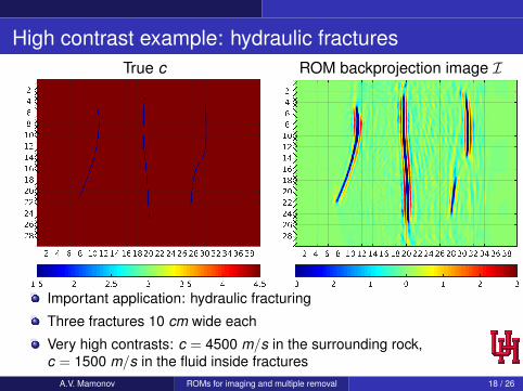
High contrast example: hydraulic fracturesTrue c ROM backprojection image I

Important application: hydraulic fracturing

Three fractures 10 cm wide each

Very high contrasts: c = 4500 m/s in the surrounding rock,c = 1500 m/s in the fluid inside fractures


Large scale example: Marmousi model


Problem 2: multiple removal

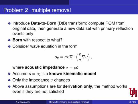
Introduce Data-to-Born (DtB) transform: compute ROM fromoriginal data, then generate a new data set with primary reflectionevents onlyBorn with respect to what?Consider wave equation in the form

utt = σc∇ ·(cσ∇u),

where acoustic impedance σ = ρcAssume c = c0 is a known kinematic modelOnly the impedance σ changesAbove assumptions are for derivation only, the method workseven if they are not satisfied


Born approximationCan show that

P ≈ I − τ2

2LqLT

q ,

whereLq = −c∇ · +

12

c∇q·, LTq = c∇+

12

c∇q,

are affine in q = log σConsider Born approximation (linearization) with respect to qaround known c = c0Perform second Cholesky factorization on ROM

2τ2 (I− P) = LqLT

q

Cholesky factors Lq, LTq are approximately affine in q, thus the

perturbationLq − L0

is approximately linear in qA.V. Mamonov ROMs for imaging and multiple removal 21 / 26

Data-to-Born transform

1 Compute P from D and P0 from D0 corresponding to q ≡ 0 (σ ≡ 1)2 Perform second Cholesky factorization, find Lq and L0

3 Form the perturbation

Lε = L0 + ε(Lq − L0), affine in εq

4 Propagate the perturbation

Dεk = BT Tk

(I− τ2

2LεLT

ε

)B

5 Differentiate to obtain DtB transformed data

Fk = D0k +

dDεk

dε

∣∣∣∣ε=0

, k = 0,1, . . . ,2n − 1


Example: DtB seismogram comparisonImpedance σ = ρc Velocity c

Original data Dk − D0k DtB transformed data Fk − D0

k


Example: DtB+RTM imaging

Impedance σ = ρc Velocity c

RTM image from original data RTM image from DtB data


Conclusions and future work

ROMs for imaging and multiple removal (DtB)Time domain formulation is essential, linear algebraic analoguesof causality: Gram-Schmidt, CholeskyImplicit orthogonalization of wavefield snapshots: removal ofmultiples in backprojection imaging and DtB transformExisting linearized imaging (RTM) and inversion (LS-RTM)methods can be applied to DtB transformed data

Future work:Data completion for partial data (including monostatic, akabackscattering measurements)Elasticity: promising preliminary resultsStability and noise effects (SVD truncation of the Gramian, etc.)Frequency domain analogue (data-driven PML)


References

1 Nonlinear seismic imaging via reduced order modelbackprojection, A.V. Mamonov, V. Druskin, M. Zaslavsky, SEGTechnical Program Expanded Abstracts 2015: pp. 4375–4379.

2 Direct, nonlinear inversion algorithm for hyperbolic problems viaprojection-based model reduction, V. Druskin, A. Mamonov, A.E.Thaler and M. Zaslavsky, SIAM Journal on Imaging Sciences9(2):684–747, 2016.

3 A nonlinear method for imaging with acoustic waves via reducedorder model backprojection, V. Druskin, A.V. Mamonov,M. Zaslavsky, 2017, arXiv:1704.06974 [math.NA]

4 Untangling the nonlinearity in inverse scattering with data-drivenreduced order models, L. Borcea, V. Druskin, A.V. Mamonov,M. Zaslavsky, 2017, arXiv:1704.08375 [math.NA]


Seismic imaging and multiple removal via model order … imaging and multiple removal via model...

Documents

Transcript of Seismic imaging and multiple removal via model order … imaging and multiple removal via model...