USE OF INTERPOLATION METHODS FOR SPATIAL CHARACTERIZATION OF

SEDIMENT CHEMICAL CONTAMINATION

A White Paper Prepared for:

Sediment Management Unit

Toxics Cleanup Program Washington Department of Ecology

Lacey, WA

Prepared by:

Maureen Goff

Science Applications International Corporation Bothell, WA

J u n e 3 0 , 2 0 0 3

SMS White Paper

TABLE OF CONTENTS

Page

1.0 INTRODUCTION................................................................................................................ 1

2.0 PROBLEM IDENTIFICATION ........................................................................................ 1

3.0 PROPOSED CLARIFICATION........................................................................................ 2

4.0 COMPARISON OF INVERSE-DISTANCE WEIGHTING AND THIESSEN POLYGONS IN ECOLOGY CASE STUDY AND RATIONALE FOR CLARIFICATION............................................................................................................... 2

4.1 Technical Advantages Of Spatial Interpolation Methods over Thiessen Polygons ....... 2

4.2 Case Study Description .................................................................................................. 4

4.3 Case Study Findings and Conclusions ........................................................................... 6

5.0 SUMMARY .......................................................................................................................... 9

LIST OF FIGURES

Figure 1: Influence of Point Distribution on Thiessen Polygons Figure 2: Examples of Multiple Grid Analyses Figure 3: Delineation of Concentration and Area by Thiessen Polygons (left) and by IDW. Figure 4: Comparison Graph of Absolute Difference (Error) of TP and IDW Acenaphthene

Estimations Figure 5: Comparison Graph of TP-Estimated Acenaphthene Values to Actual Values Figure 6: Comparison Graph of IDW-Estimated Acenaphthene Values to Actual Values

LIST OF TABLES

Table 1: SQS Exceedance Frequency for Chemical Selection Table 2: Comparison of IDW and TP Statistics and Volumes based on Point Distributions

LIST OF APPENDICES

Appendix A: IDW Algorithm Appendix B: Variography of Case Study datasets for Acenapthene, Mercury, HPAH Appendix C: Data Splitting and Estimation Error Comparison Process Appendix D: Table of Estimation Error Reports (Ex: Acenaphthene)

June 30, 2003 i

SMS White Paper

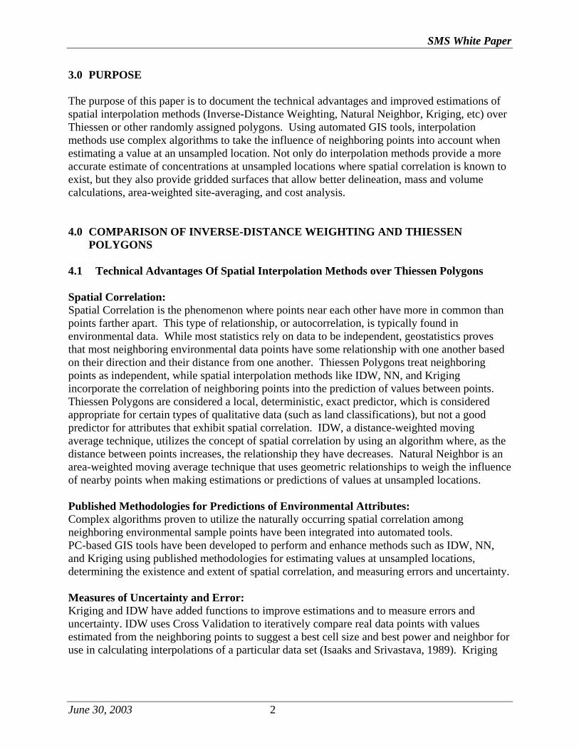
1.0 INTRODUCTION Washington State’s Sediment Management Standards (SMS) Chapter 173-204 WAC, include sediment source control and cleanup requirements to characterize the distribution of sediment chemical contamination and biological effects at any area of interest. The SMS rule also includes provisions in WAC 173-204-130(1) and (4) that mandate a goal of the use of latest scientific knowledge through the identification, review and approval of alternate technical methods deemed appropriate by the Washington State Department of Ecology (Ecology). Thiessen polygons have been a commonly used method for characterizing the distribution of sediment chemical contamination and biological effects, by assigning values to areas between sample points. Ecology now considers the alternate use of spatial interpolation methods as the latest, best science to replace the use of Thiessen or other randomly assigned polygons for characterization of the distribution of sediment chemical contamination and biological effects, area-weighted averaging, and mass and volume calculations. 2.0 PROBLEM IDENTIFICATION Thiessen polygons (TP) are often used to characterize sediments by assigning chemical concentrations or other values to areas where no actual data exists. TP’s are created by drawing straight lines equidistantly between neighboring stations and whole polygons are then assigned the sediment chemistry concentration value of the station falling within each polygon. The area of a Thiessen polygon is solely determined by the number and configuration of station points, and assigned chemistry values change abruptly at the polygon boundary (Figure 1).

Figure 1: Influence of Point Distribution on Thiessen Polygons Thiessen or other randomly assigned polygons assume neighboring sample point concentration values are independent of each other, while geostatistics prove that most environmental data is not spatially independent. Easily accessible GIS tools are now available for more advanced and robust interpolation methods that respect and utilize the spatial relationship between neighboring environmental data points.

June 30, 2003 1

SMS White Paper

3.0 PURPOSE The purpose of this paper is to document the technical advantages and improved estimations of spatial interpolation methods (Inverse-Distance Weighting, Natural Neighbor, Kriging, etc) over Thiessen or other randomly assigned polygons. Using automated GIS tools, interpolation methods use complex algorithms to take the influence of neighboring points into account when estimating a value at an unsampled location. Not only do interpolation methods provide a more accurate estimate of concentrations at unsampled locations where spatial correlation is known to exist, but they also provide gridded surfaces that allow better delineation, mass and volume calculations, area-weighted site-averaging, and cost analysis. 4.0 COMPARISON OF INVERSE-DISTANCE WEIGHTING AND THIESSEN

POLYGONS 4.1 Technical Advantages Of Spatial Interpolation Methods over Thiessen Polygons Spatial Correlation: Spatial Correlation is the phenomenon where points near each other have more in common than points farther apart. This type of relationship, or autocorrelation, is typically found in environmental data. While most statistics rely on data to be independent, geostatistics proves that most neighboring environmental data points have some relationship with one another based on their direction and their distance from one another. Thiessen Polygons treat neighboring points as independent, while spatial interpolation methods like IDW, NN, and Kriging incorporate the correlation of neighboring points into the prediction of values between points. Thiessen Polygons are considered a local, deterministic, exact predictor, which is considered appropriate for certain types of qualitative data (such as land classifications), but not a good predictor for attributes that exhibit spatial correlation. IDW, a distance-weighted moving average technique, utilizes the concept of spatial correlation by using an algorithm where, as the distance between points increases, the relationship they have decreases. Natural Neighbor is an area-weighted moving average technique that uses geometric relationships to weigh the influence of nearby points when making estimations or predictions of values at unsampled locations. Published Methodologies for Predictions of Environmental Attributes: Complex algorithms proven to utilize the naturally occurring spatial correlation among neighboring environmental sample points have been integrated into automated tools. PC-based GIS tools have been developed to perform and enhance methods such as IDW, NN, and Kriging using published methodologies for estimating values at unsampled locations, determining the existence and extent of spatial correlation, and measuring errors and uncertainty. Measures of Uncertainty and Error: Kriging and IDW have added functions to improve estimations and to measure errors and uncertainty. IDW uses Cross Validation to iteratively compare real data points with values estimated from the neighboring points to suggest a best cell size and best power and neighbor for use in calculating interpolations of a particular data set (Isaaks and Srivastava, 1989). Kriging

June 30, 2003 2

SMS White Paper

tools include variography as a first step in the interpolation to improve estimation by identifying the direction and extent of spatial correlation in a dataset. Accessibility of GIS Tools: Free Arcview Extensions developed by Region 5 EPA FIELDS Team are available for statistically-based sample design, database design and querying. FIELDS tools operating as Arcview extensions requiring Spatial Analyst include Natural Neighbor and IDW interpolations, Cross Validation for IDW, Estimation Error, Mass and Volume Calculator, and a Remediation Scenario Tool for sediment site characterization. Free stand-alone tools developed by EPA FIELDS are also available for geostatistical analysis (to determine the existence and extent of spatial correlation), Kriging, Inverse-Distance Weighting, Natural Neighbor, 3D visualization, and mass and volume calculations. Interpolated grids provide more advanced analysis opportunities and functionality: GIS grids created from interpolations provide added analysis opportunities and functionality, such as area-weighted averaging, mass and volume calculations, the ability to calculate changes over time and identify trends or multiple conditions geographically, and visualization tools like 3D and cross-sectional viewers. Area-weighted average calculations are simplified by the fact that all cells are a uniform size and have been assigned concentration values. A uniform cell size means that each cell will be given the same weight and a straight mean can be used for the area-weighted average. Therefore, grid statistics immediately report an area-weighted average with no further manual calculations. Thiessen Polygons require that each polygon be given a different weight in the averaging, by calculating the percent that each polygon contributes to the total area, multiplying that by the concentration, and then taking an average. Mass and volume calculations are performed by assigning a depth or third dimension to cells with a known area and estimated chemical concentration values. Multiple 2-dimensional grids can be used for more complex analysis such as identifying cells where multiple conditions exist, or to find changes over time in any spatially correlated data (chemistry, bathymetry, sediment thickness) on a cell-by-cell basis (Figure 2). These types of analyses cannot be done with Thiessen Polygons unless all sampling events utilize all of the same point coordinates for data collection. Figure 2: Examples of Multiple Grid Analyses

June 30, 2003 3

SMS White Paper

4.2 Case Study Description Purpose: A case study was performed to provide a quantitative measure of the increased accuracy over Thiessen Polygons with which IDW characterizes sediment chemical contaminant concentrations at unsampled locations and to demonstrate the increased functionality of working with grids versus polygons. Study Area Selection: The study area was selected based on a series of SEDQUAL queries, the Washington Department of Ecology’s sediment database and analysis tool. Selection criteria for the study area included suitable distribution and number of points for interpolation and the frequency of exceeding the Washington State Sediment Management Standards’ (SMS) Sediment Quality Standards (SQS). The study area selected was found to have a total of 68 stations, 56 stations with SQS exceedances and 35 chemicals with SQS exceedances. The points in the study area were found to have spatial correlation and distribution suitable for interpolation. Defining the Study Area Boundary: The study area had a physical barrier to the east only. Bathymetric contours were used to identify a site boundary where depth dropped off significantly enough to assume that spatial correlation might also diminish. North and South boundaries were drawn arbitrarily to include the SEDQUAL Station Locations included in the query results. Selection of Chemicals for Study Area Characterization: The Chemicals selected for characterization were chosen by ranking the SQS exceedance frequency of all chemicals found to be above their respective standards within the study area (Table 1). SEDQUAL queries reported 35 chemicals in exceedance of their SQS within the study area and three chemicals among the top ten were selected by total number of exceedances in the data:

CHEM_CD Exceedance Frequency MERCURY 77

ACENAPTHEN 34 HPAH 23

Table 1: SQS Exceedance Frequency for Chemical Selection Data: Data for the study area analysis was queried and downloaded from SEDQUAL. Because interpolations require the use of all available data (including values for non-detects if available), the data was downloaded to include all chemistry data. Data was reformatted to be compatible with FIELDS querying and modeling tools. Reformatting included changing field names and adding detection flag and detection limit fields. Data was queried using the FIELDS Query Tool for Mercury, Acenapthene, and HPAH, assigning a value of one-half the detection limit for all samples reported as non-detect. Queries were also set to select the maximum result for each

June 30, 2003 4

SMS White Paper

chemical per location if multiple values were present at a single station. FIELDS Query results were then saved as shapefiles. Existence and Extent of Spatial Correlation in the Dataset: Spatial correlation was determined through the use of FIELDS variography tools included with the Kriging interpolation function. Datasets for chemical concentrations and locations of Acenaphthene, Mercury, and HPAH were used for the geostatistical analysis. Due to the high variablility of the concentrations, all three datasets were log-normalized before performing omindirectional variography. Results for variography, found in Appendix B, were used to determine whether interpolation was suitable for these datasets, but was not used in setting the parameters of the interpolations. Interpolation Method Selection: The best interpolation method for the 3 datasets (Mercury, Acenapthene, and HPAH) was selected by running a series of both NN and of IDW interpolations using the complete datasets with all stations and running estimation error analysis. The Estimation Error FIELDS tool was used to compare the concentration value of the actual points used for interpolation with the estimated or predicted value at same coordinates. The absolute error was averaged for each chemical for both methods and compared to determine which method best represented the datasets. IDW was found to have lower estimation error with these particular datasets and was chosen as the interpolation method for the case study. Data Splitting: In order to compare the accuracy with which IDW and Thiessen Polygons (TP) estimate concentration values at unsampled locations, data was subset into two hypothetical sampling events, providing an initial sampling event dataset with which to characterize the site using the two prediction methods, and a secondary sampling event dataset with which to “groundtruth” these estimations. To randomly split the original dataset of 68 points, a sample design was created using the FIELDS Random Sample Design Tool, creating 40 points randomly distributed throughout the study area. Using Arcview Geoprocessing Tools, points from the dataset that fell closest to the randomly generated points were selected and used as “Sample Event 1 Dataset”. The remaining 28 points were used as a hypothetical, groundtruthing dataset, “Sample Event 2 Dataset”. A graphic depiction of the process is presented in Appendix C. Inverse-Distance Weighting: IDW interpolations were made from the three “Sample Event 1” datasets (Mercury, Acenapthene, and HPAH) for use in comparison to Thiessen Polygons. The interpolation parameters (Power and Neighbors), discussed in the algorithm presented in Appendix A, were selected by a combination of the Cross-Validation procedure, visual assessments of the grids, and Estimation Error Analysis. Cross-Validation runs through a process of removing points from the dataset, estimating a value for that location based on the remaining neighboring data, replacing the point and then comparing the value of that point to the value estimated for that location on the grid, resulting in all possible combinations of Power and Neighbors and the Root Mean Square Error (RMSE) associated with each combination. The lowest RMSE is the recommended combination of Power and Neighbors. A caveat presented in the FIELDS Cross-Validation Literature states: “Although empirically derived, the techniques used (for Cross-

June 30, 2003 5

SMS White Paper

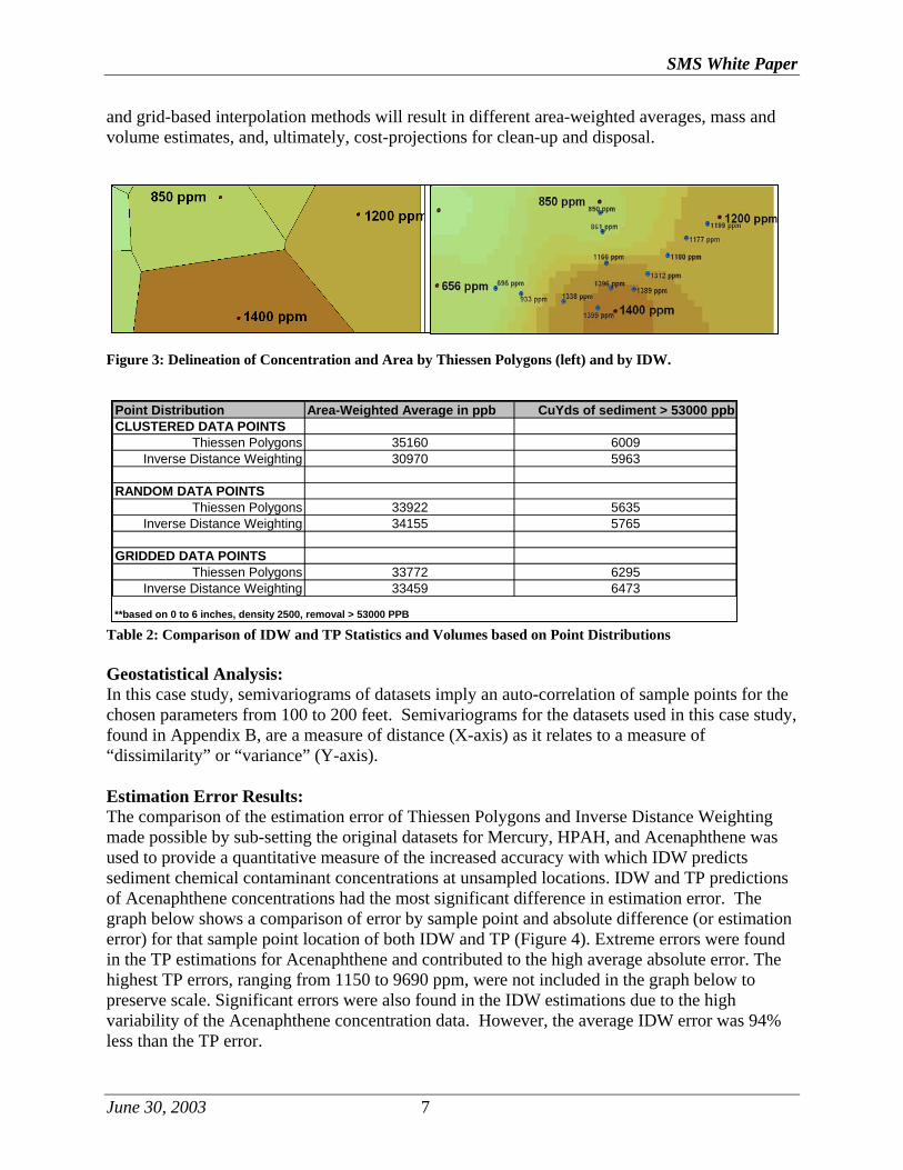
Validation) are influenced by several factors and may not always yield the best parameters for a given data set.” Therefore, the combination of Power and Neighbors with the lowest RMSE was used as a starting point for fine tuning the interpolations to reduce estimation error (using the FIELDS Estimation Error Tool) and reducing obvious flaws in the gridded surfaces detected by visual assessment of examining data points placed over the gridded surface. The Power and Neighbors chosen for the IDW interpolations were Power 3 and Neighbors 5 based on Cross-Validation, Estimation Error and visual assessments. Thiessen Polygons: Thiessen Polygons were created from the “Sample Event 1” datasets of Mercury, Acenaphthene, and HPAH concentrations using an ArcView extension. The Thiessen Polygon extension creates polygons by placing straight lines equidistantly between neighboring stations and assigning polygons the sediment chemistry concentration value of the station falling within. To make use of the Estimation Error Tool for comparing point values to estimated values, the Thiessen Polygon shapefile was converted to a grid using the same cell size and analysis extents as grids created using IDW. Estimation Error Analysis: Normally, Estimation Error Analysis is done using the point dataset with which an interpolation or grid is created. The Estimation Error Tool in FIELDS compares point values with estimated grid cell values that share the same geographic location. In this case study, the goal was to compare the accuracy with which the two methods, IDW and TP, predict values at unsampled locations. For this reason, Estimation Error Analysis was done by comparing the IDW and TP grid cells of estimated, or predicted values (created with “Sample Event 1”) to the actual values of “Sample Event 2”, (the “groundtruthing” dataset). Using the FIELDS Estimation Error Tool, the actual values of “Sample Event 2” pulled from the original dataset and reserved for this groundtruthing exercise were compared to the predicted grid cell values created by IDW and by Thiessen Polygons. An illustration of the process can be found in Step 3, Appendix C. Estimation Error Analysis reports the “Difference” and “Absolute Value Difference” of the sample point concentration value and the grid cell value in the same location. The absolute value differences of the TP grid and the IDW grid were averaged for Mercury, Acenaphthene, and HPAH. The Average Absolute Value Differences of TP and IDW were then compared for each chemical. An example of the Estimation Error Report, averaging, and comparison can be found in Appendix D. The results of the Estimation Error Analysis are discussed in the Case-Study Findings below. 4.3 Case Study Findings and Conclusions Site Characterization: Visual comparisons illustrate that Thiessen Polygons and grid-based interpolations such as IDW delineate areas and concentrations differently (Figure 3). In this particular case study, a comparison of area-weighted averages and volume calculations does not indicate that one method consistently estimates higher or lower concentration values or area. There appears to be no consistent difference or relationship in the methods by these comparisons. Thiessen polygons

June 30, 2003 6

SMS White Paper

and grid-based interpolation methods will result in different area-weighted averages, mass and volume estimates, and, ultimately, cost-projections for clean-up and disposal.

Figure 3: Delineation of Concentration and Area by Thiessen Polygons (left) and by IDW.

Point Distribution Area-Weighted Average in ppb CuYds of sediment > 53000 ppbCLUSTERED DATA POINTS

Thiessen Polygons 35160 6009Inverse Distance Weighting 30970 5963

RANDOM DATA POINTSThiessen Polygons 33922 5635

Inverse Distance Weighting 34155 5765

GRIDDED DATA POINTSThiessen Polygons 33772 6295

Inverse Distance Weighting 33459 6473

**based on 0 to 6 inches, density 2500, removal > 53000 PPB

Table 2: Comparison of IDW and TP Statistics and Volumes based on Point Distributions Geostatistical Analysis: In this case study, semivariograms of datasets imply an auto-correlation of sample points for the chosen parameters from 100 to 200 feet. Semivariograms for the datasets used in this case study, found in Appendix B, are a measure of distance (X-axis) as it relates to a measure of “dissimilarity” or “variance” (Y-axis). Estimation Error Results: The comparison of the estimation error of Thiessen Polygons and Inverse Distance Weighting made possible by sub-setting the original datasets for Mercury, HPAH, and Acenaphthene was used to provide a quantitative measure of the increased accuracy with which IDW predicts sediment chemical contaminant concentrations at unsampled locations. IDW and TP predictions of Acenaphthene concentrations had the most significant difference in estimation error. The graph below shows a comparison of error by sample point and absolute difference (or estimation error) for that sample point location of both IDW and TP (Figure 4). Extreme errors were found in the TP estimations for Acenaphthene and contributed to the high average absolute error. The highest TP errors, ranging from 1150 to 9690 ppm, were not included in the graph below to preserve scale. Significant errors were also found in the IDW estimations due to the high variability of the Acenaphthene concentration data. However, the average IDW error was 94% less than the TP error.

June 30, 2003 7

SMS White Paper

Figure 4: Comparison Graph of Absolute Difference (Error) of TP and IDW Acenaphthene Estimations Graphs comparing the predicted values generated by TP (Figure 5) and by IDW (Figure 6) to the actual values in the groundtruthing secondary sample event dataset confirm that IDW is a more accurate predictor. Complete Estimation Error Tables for Acenaphthene can be found in Appendix D.

Figure 5: Comparison Graph of TP-Estimated Acenaphthene Values to Actual Values

June 30, 2003 8

SMS White Paper

Figure 6: Comparison Graph of IDW-Estimated Acenaphthene Values to Actual Values Of the three chemical datasets chosen for this case study, all were more accurately predicted by IDW with 10 – 94% less error. Summary of Difference in Estimation Error: Mercury IDW error was 10% lower than TP Hpah IDW error was 20% lower than TP Acenaphthene IDW error was 94% lower than TP 5.0 SUMMARY For the datasets and parameters used in this case study, IDW interpolation methods proved to be a more accurate means of estimating values at unsampled sediment locations and would, therefore, give superior estimates on area, mass, volume, site-wide averages and cost. Automated GIS tools using published methodologies and algorithms to estimate values at unsampled locations provide increased accuracy, measurable error and uncertainty, and tools to reduce error by recommending interpolation parameters to fit unique datasets by the distance and direction of spatial correlation. Ecology considers the best available science for characterizing sediment chemical contamination to be interpolation methods that not only respect the spatial correlation of environmental data, but also utilize the tools that provide the greatest accuracy and provide the technical advantages of working with newly developed automated tools developed for sediment characterization.

June 30, 2003 9

SMS White Paper

References Burrough, Peter A. and McDonnell, Rachael A, Principles of Geographic Information Systems.1998. 98, 115-117. Isaaks, E.H., and Srivastava, R.M., An Introduction to Applied Geostatistics, Oxford University Press, New York, 1989. Watson, D.F. and Philip, G.M., A Refinement of Inverse Distance Weighted Interpolation, Geo-Processing, 2 .1985. 315-327. W.Tobler, 1979, "Smooth pycnophylactic interpolation for geographical regions", Journal of American Statistical Association, 74, 367:519-536 EPA QA/G-5S, December 2002, Guidance on Choosing a Sampling Design for Environmental Data Collection, p.28.

June 30, 2003 10

SMS White Paper

Appendices Appendix A IDW Algorithm Appendix B Variography of Case Study datasets for Acenaphthene, Mercury, HPAH Appendix C Data Splitting and Estimation Error Comparison Process Appendix D Table of Estimation Error Reports (Ex: Acenaphthene)

SMS White Paper

Appendix A: IDW Algorithm

G x y w f x yi i i

i

n

( , ) ( , )==∑

1

w d di ip

jp

j= − −∑/

where: G (x,y) is the IDW estimation at (x,y); f(xi,yi) is the observed value at (xi,yi); n is the number of nearest neighbors used for interpolation; wi is the weight associated with f(xi,yi); di is the distance from (x,y) to (xi,yi); and p is power, a real number. The weights are inversely related to distance and are scaled such that the sum of all the weights will add to one.

A-1

SMS White Paper

Appendix B: Variography of Case Study datasets for Acenapthene, Mercury, HPAH Semivariograms are a measure of distance (X-axis) as it relates to a measure of “dissimilarity” or “variance” (Y-axis). As the curve levels out, the dissimilarity is assumed to no longer be influenced by the distance between points and implies that spatial correlation no longer exists.

Acenaphthene - -LN transformation -Omnidirectional Mercury- -LN transformation -Omnidirectional HPAH- -LN transformation -Omnidirectional

B-1

SMS White Paper

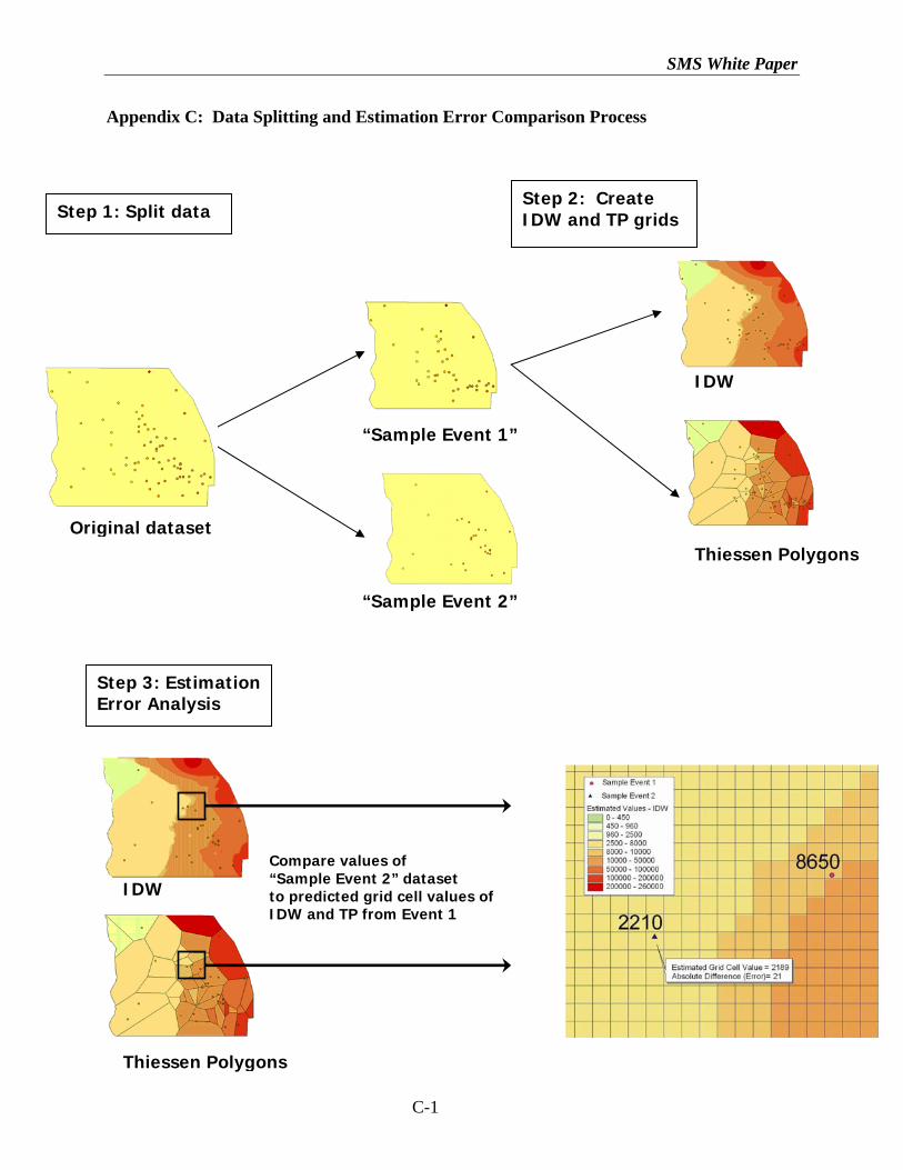
Appendix C: Data Splitting and Estimation Error Comparison Process

Step 2: Create IDW and TP grids

Step 1: Split data

Original dataset

“Sample Event 1”

IDW

Thiessen Polygons

“Sample Event 2”

Step 3: Estimation Error Analysis

Compare values of “Sample Event 2” dataset to predicted grid cell values of IDW and TP from Event 1

IDW

Thiessen Polygons

C-1

SMS White Paper

D-1

Appendix D: Table of Estimation Error Reports (Ex: Acenaphthene) Estimated Value Error of Thiessen Polygons from Sample Event 1 comparison to Actual Values of Sample Event 2 SE2 Station ID Actual Value Predicted Value Difference Absolute Difference WSF-1 490 310 -180 180 WSF-6 530 290 -240 240 P53VG6 1000 1300 300 300 VG-6 240 370 130 130 P53C4 190 2100 1910 1910 S11 100 1300 1200 1200 T1 50 97 47 47 S2 100 370 270 270 WSF-5 290 290 0 0 S0090 601.85 140 -461.85 461.85 T2 150 1300 1150 1150 P53VG4 34.53039 41.60959 7.0792 7.0792 SS-06 1000 700 -300 300 P53VG5 10000 310 -9690 9690 VG-5 490 310 -180 180 P53VG3 130 2100 1970 1970 S9 50 1300 1250 1250 P53VG6 59.96503 42 -17.96503 17.96503 P53VG2 560 140 -420 420 P53VG4 83 97 14 14 P53C2 1000 370 -630 630 VG-8 22 290 268 268 Average Absolute Error 937.9951923 Estimated Value Error of IDW from Sample Event 1 comparison to Actual Values of Sample Event 2 SE2 Station ID Actual Value Predicted Value Difference Absolute Difference WSF-1 490 490.25803 0.25803 0.25803 WSF-6 530 208.49883 -321.50117 321.50117 P53VG6 1000 999.64008 -0.35992 0.35992 VG-6 240 240.23918 0.23918 0.23918 P53C4 190 190.04152 0.04152 0.04152 S11 100 100.00552 0.00552 0.00552 T1 50 50.01418 0.01418 0.01418 S2 100 100.48309 0.48309 0.48309 WSF-5 290 265.46365 -24.53635 24.53635 S0090 601.85 601.84949 -0.00051 0.00051 T2 150 150.38959 0.38959 0.38959 P53VG4 34.53039 34.53066 0.00027 0.00027 SS-06 1000 999.99982 -0.00018 0.00018 P53VG5 10000 9999.66309 -0.33691 0.33691 VG-5 490 490.1265 0.1265 0.1265 P53VG3 130 130.11105 0.11105 0.11105 S9 50 590.60797 540.60797 540.60797 P53VG6 59.96503 77.53046 17.56543 17.56543 P53VG2 560 559.99994 -0.00006 0.00006 P53VG4 83 83.01068 0.01068 0.01068 P53C2 1000 999.94153 -0.05847 0.05847 VG-8 22 362.69498 340.69498 340.69498 Average Absolute Error 56.69734364 -93.95547609 Percent Difference in Average Absolute Error