Section 4.2

Binomial Distributions

Section 4.2 Objectives

• Determine if a probability experiment is a binomial experiment

• Find binomial probabilities using the binomial probability formula

• Graph a binomial distribution• Find the mean, variance, and standard deviation of a

binomial probability distribution

Binomial Experiments

1. The experiment is repeated for a fixed number of trials, where each trial is independent of other trials.

2. There are only two possible outcomes of interest for each trial. The outcomes can be classified as a success (S) or as a failure (F).

3. The probability of a success P(S) is the same for each trial.

4. The random variable x counts the number of successful trials.

Notation for Binomial Experiments

Symbol Description

n The number of times a trial is repeated

p = P(S) The probability of success in a single trial

q = P(F) The probability of failure in a single trial (q = 1 – p)

x The random variable represents a count of the number of successes in n trials: x = 0, 1, 2, 3, … , n.

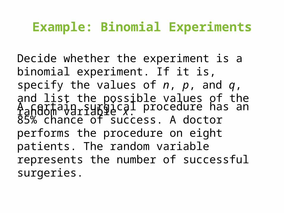
Example: Binomial Experiments

Decide whether the experiment is a binomial experiment. If it is, specify the values of n, p, and q, and list the possible values of the random variable x.

A certain surgical procedure has an 85% chance of success. A doctor performs the procedure on eight patients. The random variable represents the number of successful surgeries.

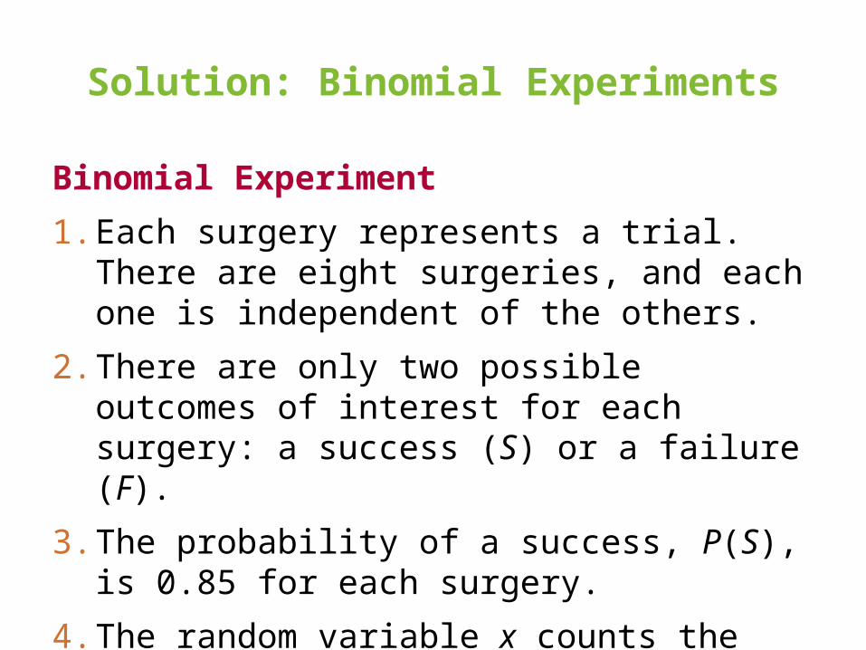
Solution: Binomial Experiments

Binomial Experiment

1. Each surgery represents a trial. There are eight surgeries, and each one is independent of the others.

2. There are only two possible outcomes of interest for each surgery: a success (S) or a failure (F).

3. The probability of a success, P(S), is 0.85 for each surgery.

4. The random variable x counts the number of successful surgeries.

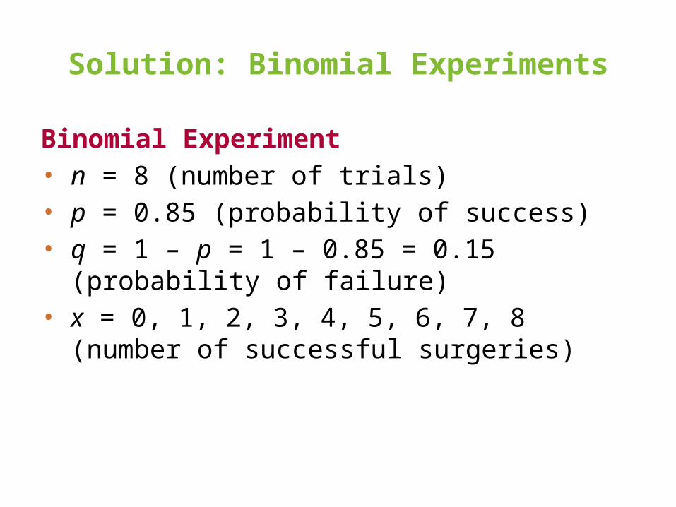
Solution: Binomial Experiments

Binomial Experiment• n = 8 (number of trials)• p = 0.85 (probability of success)• q = 1 – p = 1 – 0.85 = 0.15 (probability of failure)• x = 0, 1, 2, 3, 4, 5, 6, 7, 8 (number of successful

surgeries)

Example: Binomial Experiments

Decide whether the experiment is a binomial experiment. If it is, specify the values of n, p, and q, and list the possible values of the random variable x.

A jar contains five red marbles, nine blue marbles, and six green marbles. You randomly select three marbles from the jar, without replacement. The random variable represents the number of red marbles.

Solution: Binomial Experiments

Not a Binomial Experiment

• The probability of selecting a red marble on the first trial is 5/20.

• Because the marble is not replaced, the probability of success (red) for subsequent trials is no longer 5/20.

• The trials are not independent and the probability of a success is not the same for each trial.

Binomial Probability Formula

Binomial Probability Formula• The probability of exactly x successes in n trials is

!( )

( )! !x n x x n x

n x

nP x C p q p q

n x x

• n = number of trials• p = probability of success• q = 1 – p probability of failure• x = number of successes in n trials

Example: Finding Binomial Probabilities

Microfracture knee surgery has a 75% chance of success on patients with degenerative knees. The surgery is performed on three patients. Find the probability of the surgery being successful on exactly two patients.

Solution: Finding Binomial ProbabilitiesMethod 1: Draw a tree diagram and use the Multiplication Rule

P(2 successful surgeries) 3

9

64

0.422

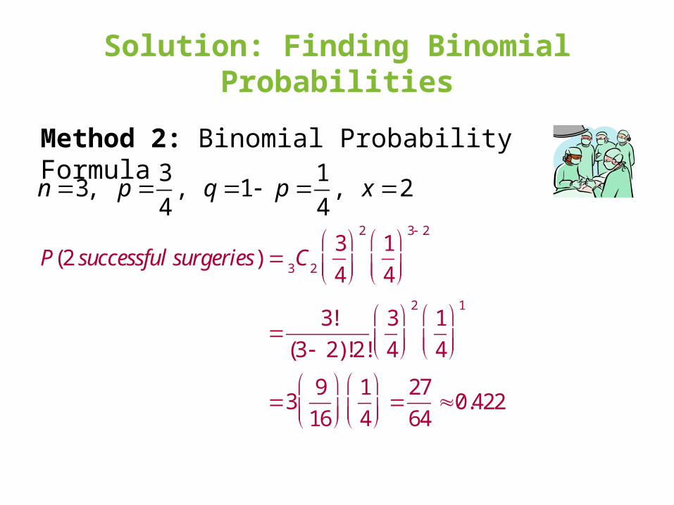
Solution: Finding Binomial Probabilities

Method 2: Binomial Probability Formula

P(2 successful surgeries) 3C

2

3

4

21

4

3 2

3!

(3 2)!2!

3

4

21

4

1

39

16

1

4

27

640.422

3 13, , 1 , 2

4 4n p q p x

Binomial Probability Distribution

Binomial Probability Distribution• List the possible values of x with the corresponding

probability of each.• Example: Binomial probability distribution for

Microfracture knee surgery: n = 3, p =

Use the binomial probability formula to find probabilities.

x 0 1 2 3

P(x) 0.016 0.141 0.422 0.422

3

4

Example: Constructing a Binomial Distribution

In a survey, U.S. adults were asked to give reasons why they liked texting on their cellular phones. Seven adults who participated in the survey are randomly selected and asked whether they like texting because it is quicker thancalling. Create a binomial probability distribution for the number of adults who respond yes.

Solution: Constructing a Binomial Distribution

• 56% of adults like texting because it is quicker than calling.

• n = 7, p = 0.56, q = 0.44, x = 0, 1, 2, 3, 4, 5, 6, 7

P(0) = 7C0(0.56)0(0.44)7 = 1(0.56)0(0.44)7 ≈ 0.0032

P(1) = 7C1(0.56)1(0.44)6 = 7(0.56)1(0.44)6 ≈ 0.0284

P(2) = 7C2(0.56)2(0.44)5 = 21(0.56)2(0.44)5 ≈ 0.1086

P(3) = 7C3(0.56)3(0.44)4 = 35(0.56)3(0.44)4 ≈ 0.2304

P(4) = 7C4(0.56)4(0.44)3 = 35(0.56)4(0.44)3 ≈ 0.2932

P(5) = 7C5(0.56)5(0.44)2 = 21(0.56)5(0.44)2 ≈ 0.2239

P(6) = 7C6(0.56)6(0.44)1 = 7(0.56)6(0.44)1 ≈ 0.0950

P(7) = 7C7(0.56)7(0.44)0 = 1(0.56)7(0.44)0 ≈ 0.0173

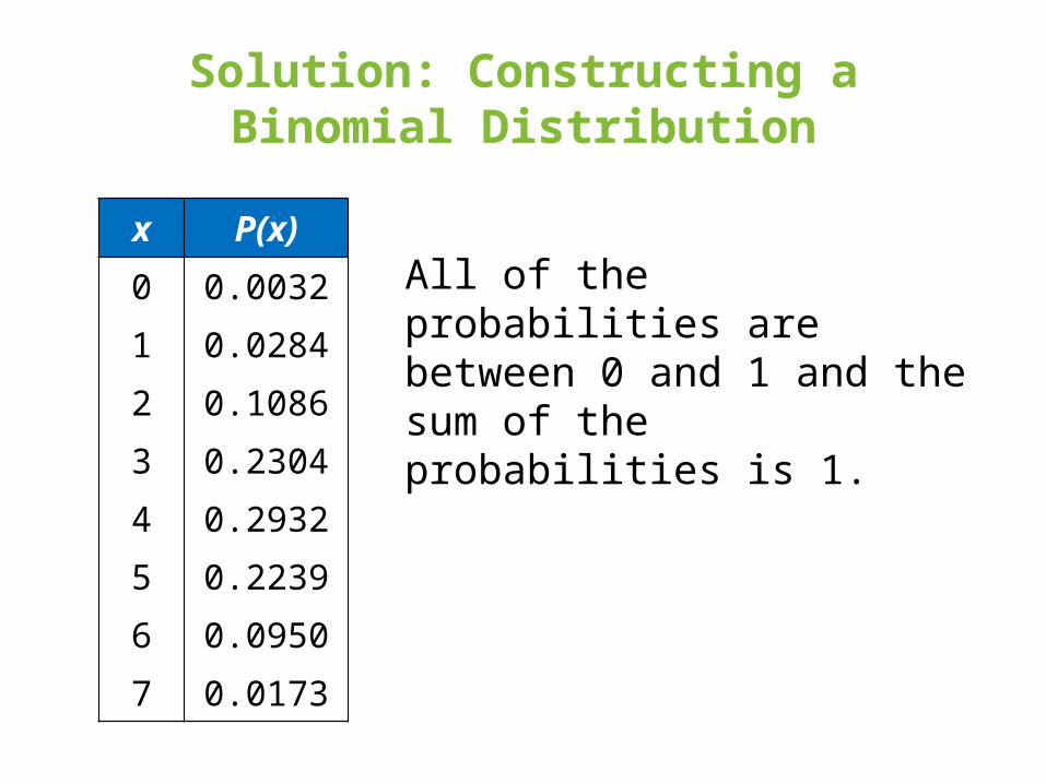
Solution: Constructing a Binomial Distribution

x P(x)

0 0.0032

1 0.0284

2 0.1086

3 0.2304

4 0.2932

5 0.2239

6 0.0950

7 0.0173

All of the probabilities are between 0 and 1 and the sum of the probabilities is 1.

Example: Finding Binomial Probabilities

A survey indicates that 41% of women in the U.S. consider reading their favorite leisure-time activity. You randomly select four U.S. women and ask them if reading is their favorite leisure-time activity. Find the probability that at least two of them respond yes.

Solution: • n = 4, p = 0.41, q = 0.59• At least two means two or more.• Find the sum of P(2), P(3), and P(4).

Solution: Finding Binomial Probabilities

P(2) = 4C2(0.41)2(0.59)2 = 6(0.41)2(0.59)2 ≈ 0.351094

P(3) = 4C3(0.41)3(0.59)1 = 4(0.41)3(0.59)1 ≈ 0.162654

P(4) = 4C4(0.41)4(0.59)0 = 1(0.41)4(0.59)0 ≈ 0.028258

(any_value)0 = 1

P(x ≥ 2) = P(2) + P(3) + P(4) ≈ 0.351094 + 0.162654 + 0.028258 ≈ 0.542

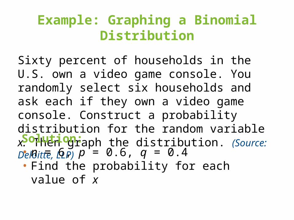
Example: Graphing a Binomial Distribution

Sixty percent of households in the U.S. own a video game console. You randomly select six households and ask each if they own a video game console. Construct a probability distribution for the random variable x. Then graph the distribution. (Source: Deloitte, LLP)

Solution: • n = 6, p = 0.6, q = 0.4• Find the probability for each value of x

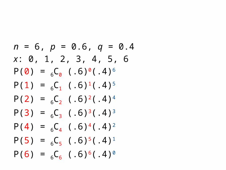
n = 6, p = 0.6, q = 0.4

x: 0, 1, 2, 3, 4, 5, 6

P(0) = 6C0 (.6)0(.4)6

P(1) = 6C1 (.6)1(.4)5

P(2) = 6C2 (.6)2(.4)4

P(3) = 6C3 (.6)3(.4)3

P(4) = 6C4 (.6)4(.4)2

P(5) = 6C5 (.6)5(.4)1

P(6) = 6C6 (.6)6(.4)0

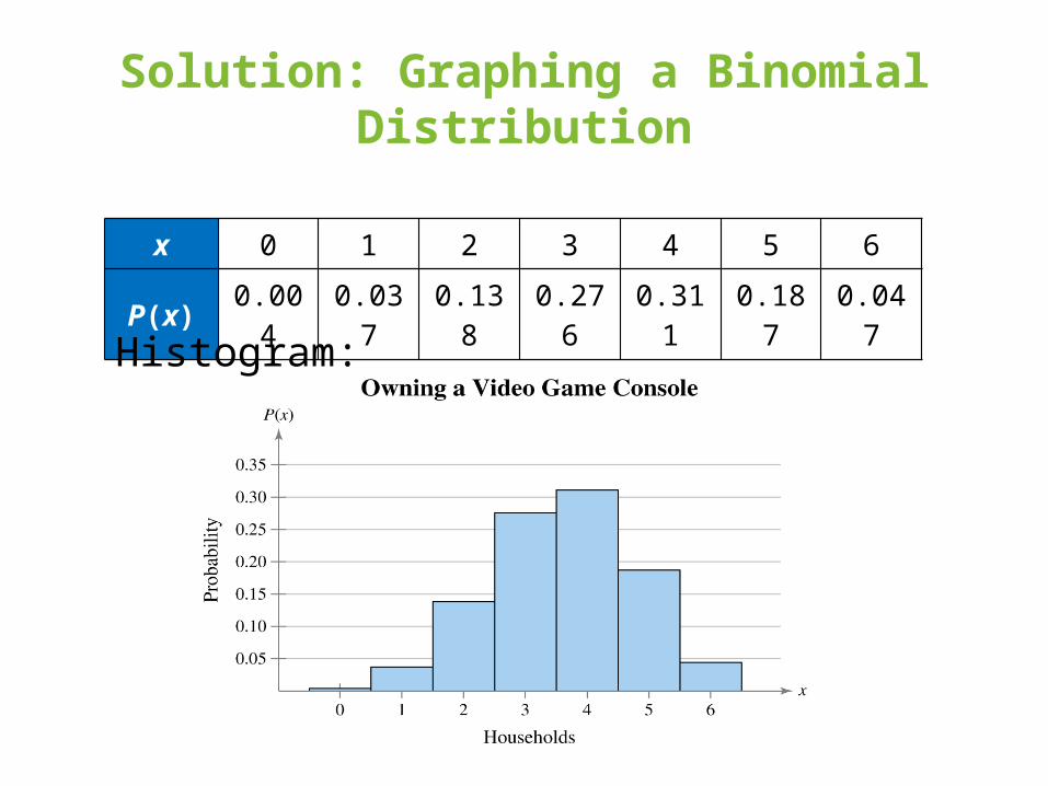
Solution: Graphing a Binomial Distribution

x 0 1 2 3 4 5 6

P(x) 0.004 0.037 0.138 0.276 0.311 0.187 0.047

Histogram:

Mean, Variance, and Standard Deviation

• Mean: μ = np

• Variance: σ2 = npq

• Standard Deviation: npq

Example: Finding the Mean, Variance, and Standard Deviation

In Pittsburgh, Pennsylvania, about 56% of the days in a year are cloudy. Find the mean, variance, and standard deviation for the number of cloudy days during the month of June. Interpret the results and determine any unusual values. (Source: National Climatic Data Center)

Solution: n = 30, p = 0.56, q = 0.44

Mean: μ = np = 30∙0.56 = 16.8Variance: σ2 = npq = 30∙0.56∙0.44 ≈ 7.4Standard Deviation: 30 0.56 0.44 2.7npq

Solution: Finding the Mean, Variance, and Standard Deviation

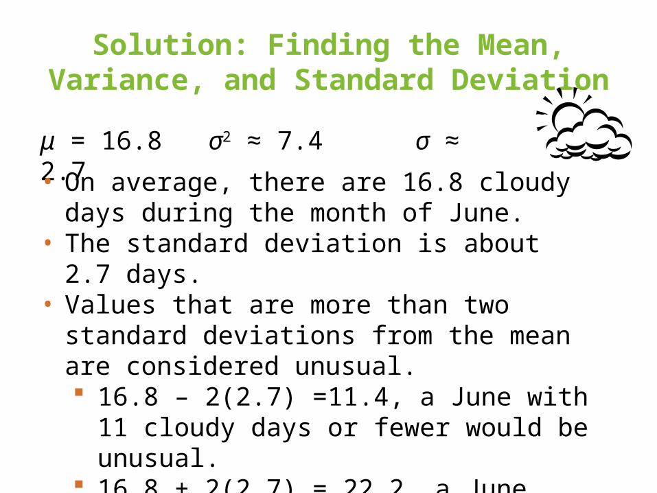
μ = 16.8 σ2 ≈ 7.4 σ ≈ 2.7

• On average, there are 16.8 cloudy days during the month of June.

• The standard deviation is about 2.7 days. • Values that are more than two standard deviations

from the mean are considered unusual. 16.8 – 2(2.7) =11.4, a June with 11 cloudy days

or fewer would be unusual. 16.8 + 2(2.7) = 22.2, a June with 23 cloudy days

or more would also be unusual.

Section 4.2 Summary

• Determined if a probability experiment is a binomial experiment

• Found binomial probabilities using the binomial probability formula

• Graphed a binomial distribution• Found the mean, variance, and standard deviation of

a binomial probability distribution