Section 4.2 Binomial Distributions Larson/Farber 4th ed 1.
28
Section 4.2 Binomial Distributions Larson/Farber 4th ed 1
-
Upload
warren-obrien -
Category
Documents
-
view
225 -
download
2
Transcript of Section 4.2 Binomial Distributions Larson/Farber 4th ed 1.
Section 4.2
Binomial Distributions
Larson/Farber 4th ed 1
Section 4.2 Objectives
• Determine if a probability experiment is a binomial experiment
• Find binomial probabilities using the binomial probability formula
• Find binomial probabilities using a binomial table
• Graph a binomial distribution
• Find the mean, variance, and standard deviation of a binomial probability distribution
Larson/Farber 4th ed 2
Binomial Experiments
1. The experiment is repeated for a fixed number of trials, where each trial is independent of other trials.
2. There are only two possible outcomes of interest for each trial. The outcomes can be classified as a success (S) or as a failure (F).
3. The probability of a success P(S) is the same for each trial.
4. The random variable x counts the number of successful trials.
Larson/Farber 4th ed 3
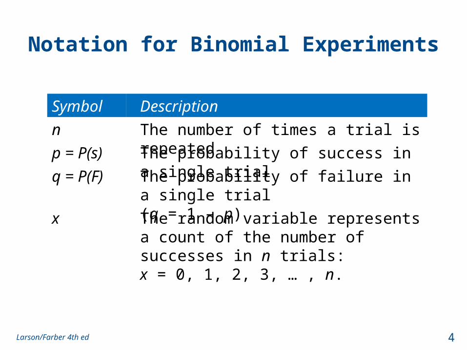
Notation for Binomial Experiments
Symbol Description
n The number of times a trial is repeated
p = P(s) The probability of success in a single trial
q = P(F) The probability of failure in a single trial (q = 1 – p)
x The random variable represents a count of the number of successes in n trials: x = 0, 1, 2, 3, … , n.
Larson/Farber 4th ed 4
Example: Binomial Experiments
Decide whether the experiment is a binomial experiment. If it is, specify the values of n, p, and q, and list the possible values of the random variable x.
Larson/Farber 4th ed 5
1. A certain surgical procedure has an 85% chance of success. A doctor performs the procedure on eight patients. The random variable represents the number of successful surgeries.
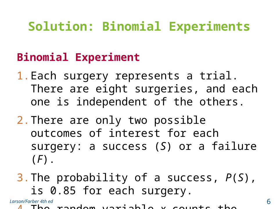
Solution: Binomial Experiments
Binomial Experiment
1. Each surgery represents a trial. There are eight surgeries, and each one is independent of the others.
2. There are only two possible outcomes of interest for each surgery: a success (S) or a failure (F).
3. The probability of a success, P(S), is 0.85 for each surgery.
4. The random variable x counts the number of successful surgeries.
Larson/Farber 4th ed 6
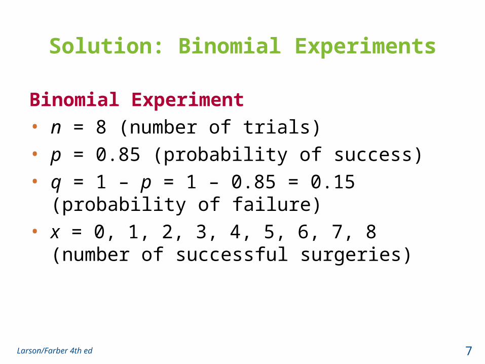
Solution: Binomial Experiments
Binomial Experiment
• n = 8 (number of trials)
• p = 0.85 (probability of success)
• q = 1 – p = 1 – 0.85 = 0.15 (probability of failure)
• x = 0, 1, 2, 3, 4, 5, 6, 7, 8 (number of successful surgeries)
Larson/Farber 4th ed 7
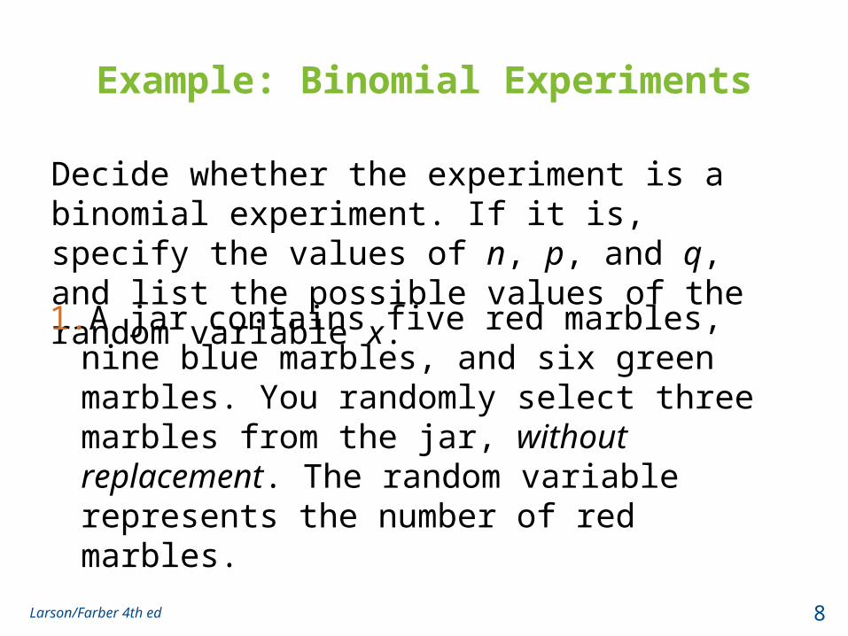
Example: Binomial Experiments
Decide whether the experiment is a binomial experiment. If it is, specify the values of n, p, and q, and list the possible values of the random variable x.
Larson/Farber 4th ed 8
1. A jar contains five red marbles, nine blue marbles, and six green marbles. You randomly select three marbles from the jar, without replacement. The random variable represents the number of red marbles.
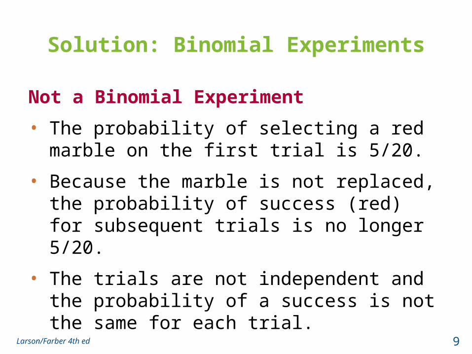
Solution: Binomial Experiments
Not a Binomial Experiment
• The probability of selecting a red marble on the first trial is 5/20.
• Because the marble is not replaced, the probability of success (red) for subsequent trials is no longer 5/20.
• The trials are not independent and the probability of a success is not the same for each trial.
Larson/Farber 4th ed 9
Binomial Probability Formula
10Larson/Farber 4th ed
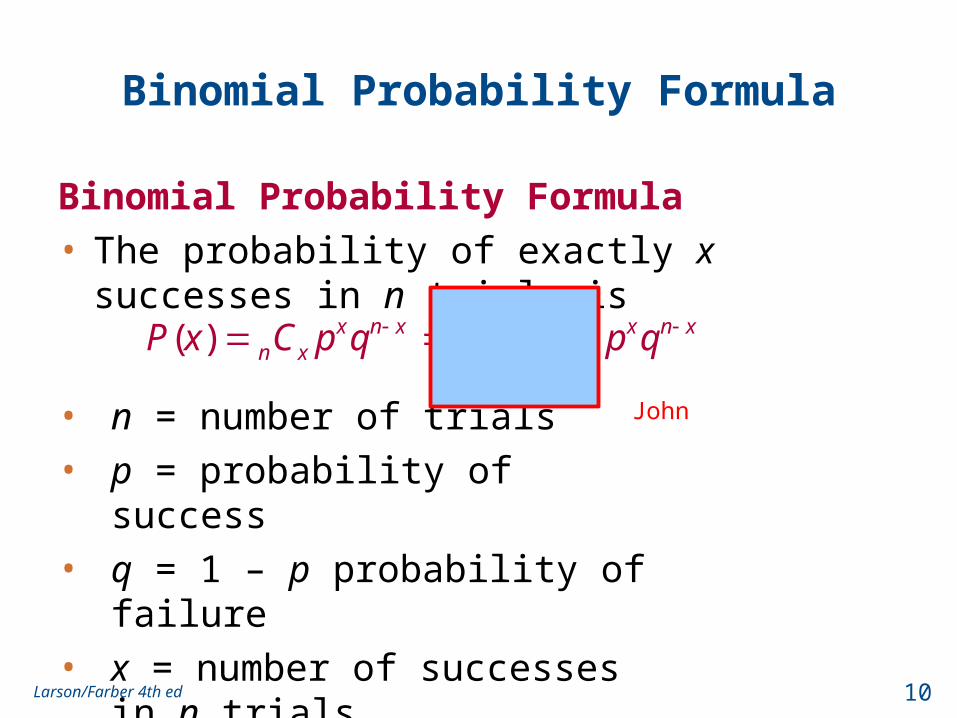
Binomial Probability Formula
• The probability of exactly x successes in n trials is
!( )
( )! !x n x x n x
n x
nP x C p q p q
n x x
• n = number of trials
• p = probability of success
• q = 1 – p probability of failure
• x = number of successes in n trials
John
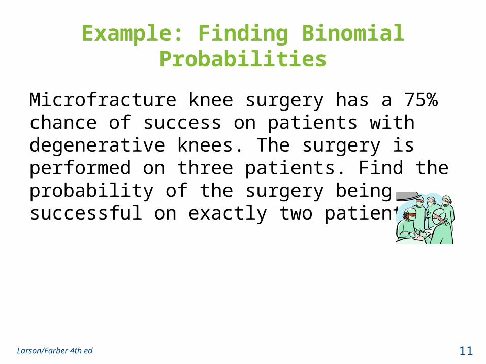
Example: Finding Binomial Probabilities
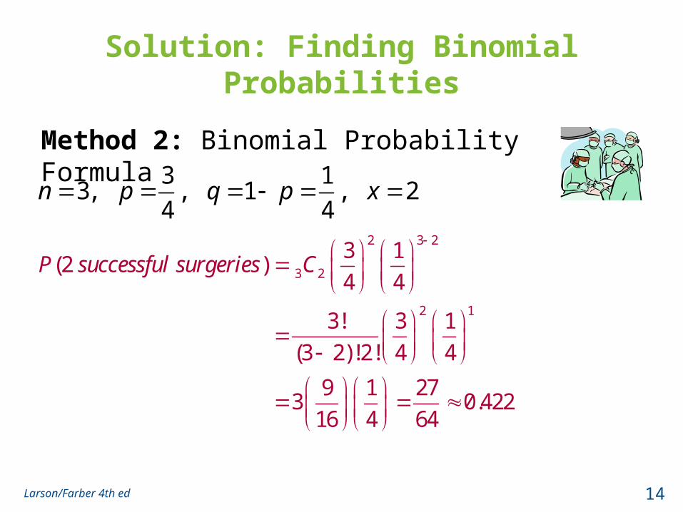
Microfracture knee surgery has a 75% chance of success on patients with degenerative knees. The surgery is performed on three patients. Find the probability of the surgery being successful on exactly two patients.
Larson/Farber 4th ed 11
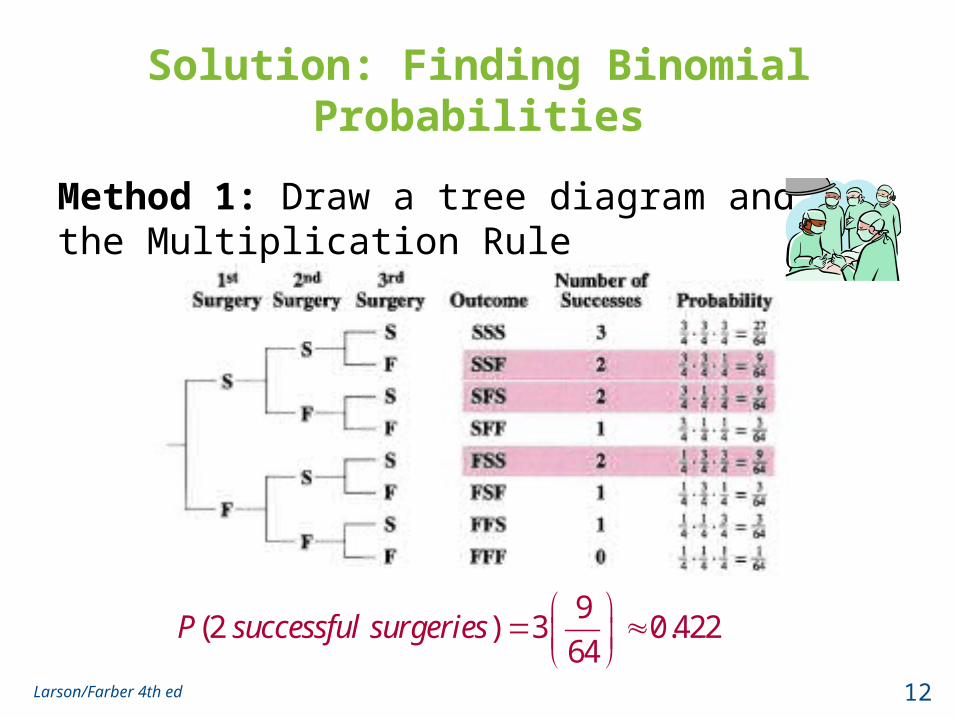
Solution: Finding Binomial Probabilities
Method 1: Draw a tree diagram and use the Multiplication Rule
Larson/Farber 4th ed 12
9(2 ) 3 0.422
64P successful surgeries
Are you here? Are you listening?
Ten percent of adults say oatmeal cookies are their favorite cookie. You select 2 people to ask. What is the probability that exactly 1 of them will say that oatmeal cookies are their favorite?
Solution: Finding Binomial Probabilities
Method 2: Binomial Probability Formula
Larson/Farber 4th ed 14
2 3 2
3 2
2 1
3 1(2 )
4 4
3! 3 1
(3 2)!2! 4 4
9 1 273 0.422
16 4 64
P successful surgeries C
3 13, , 1 , 2
4 4n p q p x
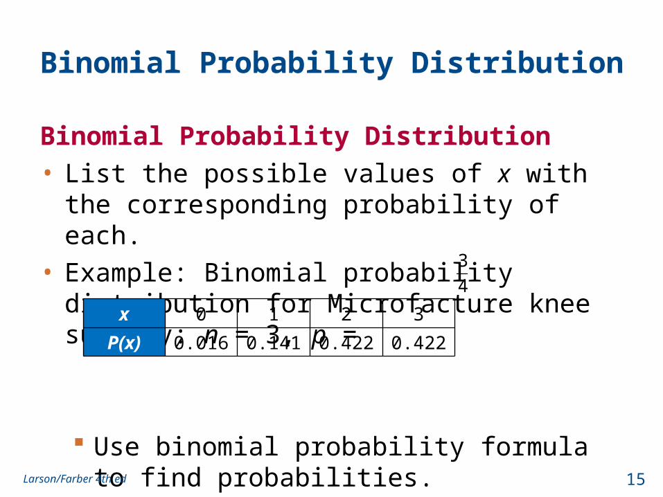
Binomial Probability Distribution
Binomial Probability Distribution
• List the possible values of x with the corresponding probability of each.
• Example: Binomial probability distribution for Microfacture knee surgery: n = 3, p =
Use binomial probability formula to find probabilities.
Larson/Farber 4th ed 15
x 0 1 2 3
P(x) 0.016 0.141 0.422 0.422
3
4

Example: Constructing a Binomial Distribution
In a survey, workers in the U.S. were asked to name their expected sources of retirement income. Seven workers who participated in the survey are randomly selected and asked whether they expect to rely on Social
Larson/Farber 4th ed 16
Security for retirement income. Create a binomial probability distribution for the number of workers who respond yes.
Solution: Constructing a Binomial Distribution
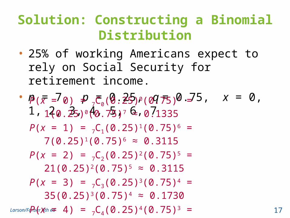
• 25% of working Americans expect to rely on Social Security for retirement income.
• n = 7, p = 0.25, q = 0.75, x = 0, 1, 2, 3, 4, 5, 6, 7
Larson/Farber 4th ed 17
P(x = 0) = 7C0(0.25)0(0.75)7 = 1(0.25)0(0.75)7 ≈ 0.1335
P(x = 1) = 7C1(0.25)1(0.75)6 = 7(0.25)1(0.75)6 ≈ 0.3115
P(x = 2) = 7C2(0.25)2(0.75)5 = 21(0.25)2(0.75)5 ≈ 0.3115
P(x = 3) = 7C3(0.25)3(0.75)4 = 35(0.25)3(0.75)4 ≈ 0.1730
P(x = 4) = 7C4(0.25)4(0.75)3 = 35(0.25)4(0.75)3 ≈ 0.0577
P(x = 5) = 7C5(0.25)5(0.75)2 = 21(0.25)5(0.75)2 ≈ 0.0115
P(x = 6) = 7C6(0.25)6(0.75)1 = 7(0.25)6(0.75)1 ≈ 0.0013
P(x = 7) = 7C7(0.25)7(0.75)0 = 1(0.25)7(0.75)0 ≈ 0.0001
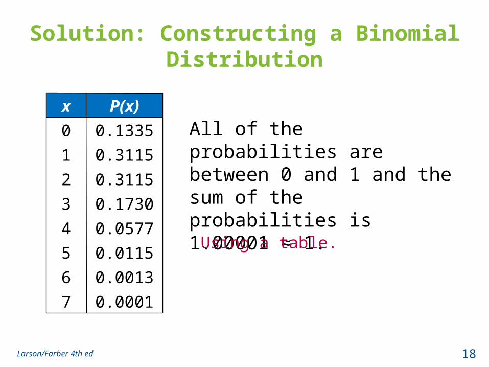
Solution: Constructing a Binomial Distribution
Larson/Farber 4th ed 18
x P(x)
0 0.1335
1 0.3115
2 0.3115
3 0.1730
4 0.0577
5 0.0115
6 0.0013
7 0.0001
All of the probabilities are between 0 and 1 and the sum of the probabilities is 1.00001 ≈ 1.
Using a table.
Example: Finding Binomial Probabilities
A survey indicates that 40% of women in the U.S. consider reading their favorite leisure-time activity. You randomly select four U.S. women and ask them if reading is their favorite leisure-time activity. Find the probability that at least two of them respond yes.
Larson/Farber 4th ed 19
Solution: • n = 4, p = 0.40, q = 0.60• At least two means two or more.• Find the sum of P(2), P(3), and P(4).
Solution: Finding Binomial Probabilities
Larson/Farber 4th ed 20
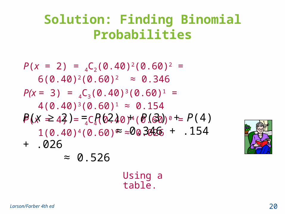
P(x = 2) = 4C2(0.40)2(0.60)2 = 6(0.40)2(0.60)2 ≈ 0.346
P(x = 3) = 4C3(0.40)3(0.60)1 = 4(0.40)3(0.60)1 ≈ 0.154
P(x = 4) = 4C4(0.40)4(0.60)0 = 1(0.40)4(0.60)0 ≈ 0.026
P(x ≥ 2) = P(2) + P(3) + P(4) ≈ 0.346 + .154 + .026 ≈ 0.526
Using a table.
Example: Finding Binomial Probabilities Using a Table
About thirty percent of working adults spend less than 15 minutes each way commuting to their jobs. You randomly select six working adults. What is the probability that exactly three of them spend less than 15 minutes each way commuting to work? Use a table to find the probability. (Source: U.S. Census Bureau)
Larson/Farber 4th ed 21
Solution:• Binomial with n = 6, p = 0.30, x = 3
Solution: Finding Binomial Probabilities Using a Table
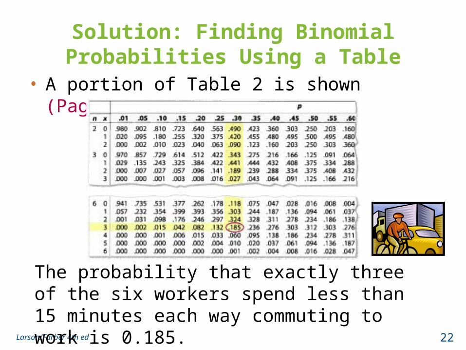
• A portion of Table 2 is shown (Page A8 - A10)
Larson/Farber 4th ed 22
The probability that exactly three of the six workers spend less than 15 minutes each way commuting to work is 0.185.
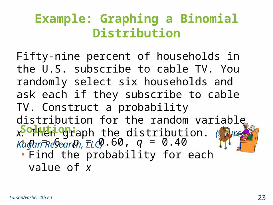
Example: Graphing a Binomial Distribution
Fifty-nine percent of households in the U.S. subscribe to cable TV. You randomly select six households and ask each if they subscribe to cable TV. Construct a probability distribution for the random variable x. Then graph the distribution. (Source: Kagan Research, LLC)
Larson/Farber 4th ed 23
Solution: • n = 6, p = 0.60, q = 0.40• Find the probability for each value of x
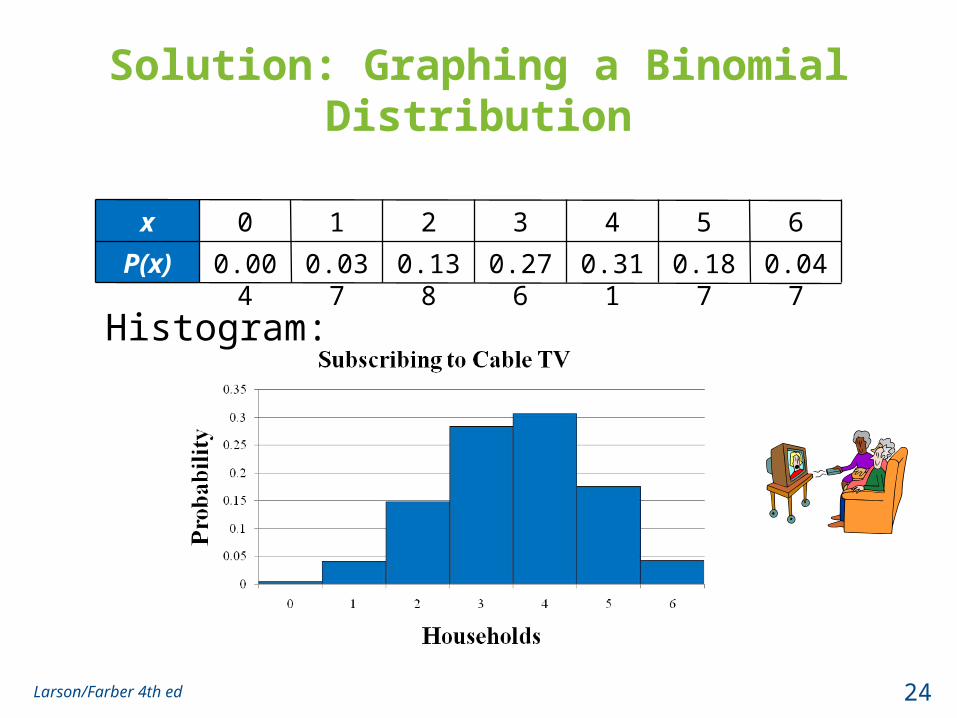
Solution: Graphing a Binomial Distribution
Larson/Farber 4th ed 24
x 0 1 2 3 4 5 6
P(x) 0.004 0.037 0.138 0.276 0.311 0.187 0.047
Histogram:
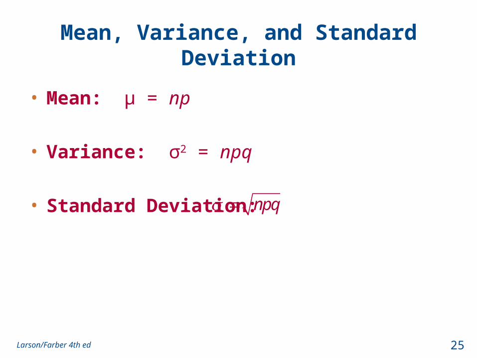
Mean, Variance, and Standard Deviation
• Mean: μ = np
• Variance: σ2 = npq
• Standard Deviation:
Larson/Farber 4th ed 25
npq
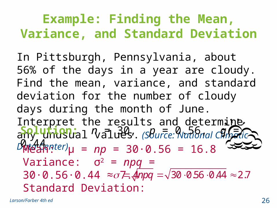
Example: Finding the Mean, Variance, and Standard Deviation
In Pittsburgh, Pennsylvania, about 56% of the days in a year are cloudy. Find the mean, variance, and standard deviation for the number of cloudy days during the month of June. Interpret the results and determine any unusual values. (Source: National Climatic Data Center)
Larson/Farber 4th ed 26
Solution: n = 30, p = 0.56, q = 0.44
Mean: μ = np = 30∙0.56 = 16.8Variance: σ2 = npq = 30∙0.56∙0.44 ≈ 7.4Standard Deviation: 30 0.56 0.44 2.7npq
Solution: Finding the Mean, Variance, and Standard Deviation
Larson/Farber 4th ed 27
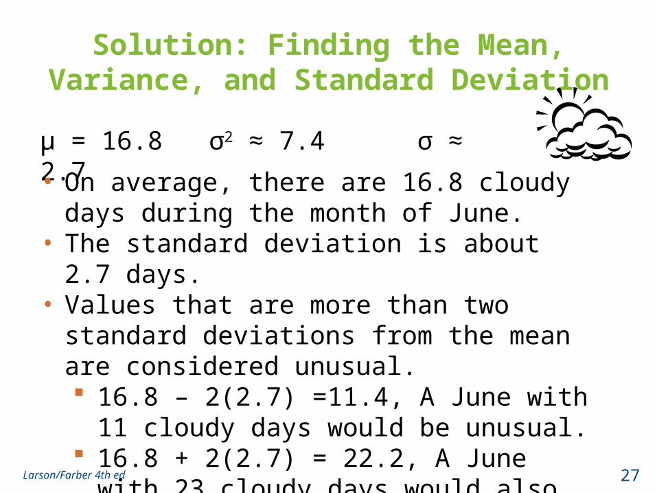
μ = 16.8 σ2 ≈ 7.4 σ ≈ 2.7
• On average, there are 16.8 cloudy days during the month of June.
• The standard deviation is about 2.7 days. • Values that are more than two standard deviations
from the mean are considered unusual. 16.8 – 2(2.7) =11.4, A June with 11 cloudy days
would be unusual. 16.8 + 2(2.7) = 22.2, A June with 23 cloudy
days would also be unusual.
Section 4.2 Summary
• Determined if a probability experiment is a binomial experiment
• Found binomial probabilities using the binomial probability formula
• Found binomial probabilities using technology and a binomial table
• Graphed a binomial distribution
• Found the mean, variance, and standard deviation of a binomial probability distribution
Larson/Farber 4th ed 28