Section 3.7 Suppose the number of occurrences in a “unit” interval follows a Poisson...

Section 3.7

Suppose the number of occurrences in a “unit” interval follows a Poisson distribution with mean .

Recall that for w > 0,P(interval length to obtain the first occurrence w) =1 – P(interval length to obtain the first occurrence > w) =1 – P(no occurrences in interval of length w) = .

Consider a random variableW = interval length to obtain the first occurrence

with distribution function G(w) = P(W w) = 1 – e–H(w) for w > 0 , where

H(w) =

(phone calls) (one hour)

(10 phone calls per hour)

1 – e–w

0

w

(t) dt .

If the function (t) is a constant, say , then H(w) = , so that the p.d.f. of W is

g(w) =

which is the p.d.f. for an distribution.

A non-constant function (t) implies that the mean of the Poisson process changes over an interval. For instance, the number of occurrences in a “unit” interval may steadily increase (or decrease).

We observe that in general, H /(w) = , so that the p.d.f. of W is

g(w) =

When W represents length of life (for an item or living organism), (w) is called the failure rate or force of mortality, and we find that

(w) =

If H(w) = for > 0 and > 0, we say W has a Weibull distribution.

exponential( ) 1—

w

e–w if w > 0 ,

(phone calls per hour) (increase as time goes on)

(w)

H /(w)e–H(w) = (w)e–H(w) if w > 0 .

g(w)—— =e–H(w)

g(w)———— .1 – G(w)

w—

1.

H(w) = in order to demonstrate that W has a Weibull

distribution.

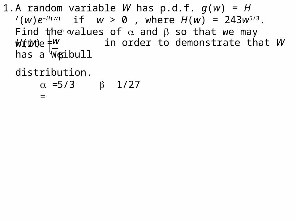
A random variable W has p.d.f. g(w) = H /(w)e–H(w) if w > 0 , where H(w) = 243w5/3. Find the values of and so that we may write

w—

= =5/3 1/27

2.

(a) Find the distribution function for W.

Suppose the random variable W represents length of life and has p.d.f. g(w) = H /(w)e–H(w) if w > 0 , with an exponential force of mortality

(w) = for a > 0 and b > 0. g(w)———— = aebw

1 – G(w)

0

w

(t) dt =H(w) =

0

w

aebt dt =aebw – a——— b

The distribution function for W is G(w) =

if w 0

if 0 < w

0

1 – expa – aebw

——— b

(b) Find the p.d.f. for W (known as Gompertz law).

if w > 0 .The p.d.f. for W is g(w) = aebw expa – aebw

——— b

Let X be a random variable with c.d.f. F(x). In general, for any value v, P(X = v) = P(X v) P(X < v) = P(X v) Lim P(X x) =

x v

F(v) Lim F(v) .x v

Example. Let X be a random variable with c.d.f. F(x) =

0 if x < 5

1/4 if 5 x < 6

(x 5) / 4 if 6 x < 9

1 if 9 x

5

1/4

0

1/2

3/4

1

6 7 8 9

Suppose v is a value less than 5, say 4.8.P(X = v) = P(X = 4.8) =F(4.8) Lim F(x) =

x 4.80 0 = 0


0 if x < 5

1/4 if 5 x < 6

(x 5) / 4 if 6 x < 9

1 if 9 x

5

1/4

0

1/2

3/4

1

6 7 8 9

Suppose v is 5.P(X = v) = P(X = 5) =F(5) Lim F(x) =

x 51/4 0 = 1/4

Suppose v is a value greater than 5 but less than 6, say 5.8.P(X = v) = P(X = 5.8) =F(5.8) Lim F(x) =

x 5.81/4 1/4 = 0


0 if x < 5

1/4 if 5 x < 6

(x 5) / 4 if 6 x < 9

1 if 9 x

5

1/4

0

1/2

3/4

1

6 7 8 9

Suppose v is a value such that 6 v < 9, say 7.5.P(X = v) = P(X = 7.5) =F(7.5) Lim F(x) =

x 7.5

5 / 8 (7.5 5) / 4 = 0

Suppose v is a value greater than or equal to 9, say 9.8.P(X = v) = P(X = 9.8) =F(9.8) Lim F(x) =

x 9.81 1 = 0


0 if x < 5

1/4 if 5 x < 6

(x 5) / 4 if 6 x < 9

1 if 9 x

5

1/4

0

1/2

3/4

1

6 7 8 9

Consequently, we see thatif v 5, then P(X = v) = 0 but P(X = 5) =1 / 4

We also see that P(6 < X 9) = P(X 9) P(X 6) =F(9) F(6) = 1 1 / 4 = 3 / 4

We see then that the space of X is {5} {x | 6 < x < 9}

We see then that the space of X is {5} {x | 6 < x < 9}

What kind of random variable X could have this space?A dart is thrown at a circular board of radius 9 inches. If the dart lands in the area between 3 and 9 inches from the center, a score of 6 is assigned; if the dart lands within 3 inches of the center, then a score of 9 x is assigned where x is the distance from the center.

Blue Area Score = 9 x where x = inches from the center.

Yellow Area Score = 6

The random variable X is not a discrete type random variable and is not a continuous type random variable; X is called a random variable of the mixed type.

Let F(x) be the distribution function for a random variable X, then (1) F(x) must be an function, (2) as x –, F(x) , and (3) as x +, F(x) .

If there exists a discrete set of points at which F(x) is discontinuous with F /(x) = 0 at all other points, then X must be a type random variable whose space is the set of points of discontinuity. (The probability of observing a given value in the space of X is equal to the “length of the jump in F(x)” at the given value.)

increasing 01

discrete

If F(x) is continuous everywhere, then X is a type random variable whose space is the set of points where F /(x) > 0 (i.e., the set of points where F(x) is strictly increasing).

continuous

If there exists a discrete set of points at which F(x) is discontinuous and also one or more intervals where F /(x) > 0, then X is called a random variable of the mixed type. Such a random variable is neither of the discrete type or the continuous type and has no p.m.f. or p.d.f. The space of X consists of the union of the set of points of discontinuity and the intervals where F /(x) > 0.

3.

(a)

For each distribution function, (1) sketch a graph, and (2) either find the corresponding p.m.f. or p.d.f., or state why no p.m.f. or p.d.f. can be found.

1X1 has distribution function F1(x) = 1 – ——— if – < x < .

(1 + ex)

0

1/2

1

X1 is a continuous type random variable with p.d.f. f1(x) = F1(x) =

ex

——— if – < x < .(1 + ex)2

(b) X2 has distribution function F2(x) =

0 if x < – 3

(x3 + 27) / 35 if – 3 x < 2

1 if 2 x

0– 3

1

2

X2 is a continuous type random variable with p.d.f. f2(x) = F2(x) =

3x2

— if – 3 x < 2 .35

(c) X3 has distribution function F3(x) =

0 if x < – 2

1/6 if – 2 x < 0

1/3 if 0 x < 2

2/3 if 2 x < 4

11/12 if 4 x < 6

1 if 6 x

0– 2

1

2

1/61/3

2/3

4

11/12

6

X3 is a discrete type random variable. The space of X is The p.m.f. of X is f3(x) ={– 2, 0, 2, 4, 6}.

1/6 if x = – 21/6 if x = 01/3 if x = 21/4 if x = 41/12 if x = 6

(d) X4 has distribution function F4(x) =

0 if x < – 2

(x + 2) / 12 if – 2 x < 0

(2 + 3x ) / 12 if 0 x < 4

11 / 12 if 4 x < 5

1 if 5 x

0– 2

1

2

1/6

2/3

4

11/12

5

X4 has a distribution of the mixed type. X4 has no p.m.f. or p.d.f. The space of X4 is {x | – 2 < x < 4} {4,5}.

(e) X5 has distribution function F5(x) =

0 if x < – 2

(x + 2) / 12 if – 2 x < 0

(5 + 3x ) / 12 if 0 x < 4

11 / 12 if 4 x < 5

1 if 5 x

0– 2

1

2

1/6

5/12

4

11/12

5

X5 has a distribution of the mixed type. X5 has no p.m.f. or p.d.f. The space of X5 is {x | – 2 < x < 0} {0} {x | 0 < x < 4}

{5}.

4.

(a)

An urn contains one chip labeled with *, two chips each labeled with **, and three chips each labeled with ***. The random variables Y1 and Y2 have respective U(–1,0) and U(0,1) distributions. One chip is randomly selected and the following random variable is observed:

Find the distribution function of X.

Y1 if the chip selected is labeled with **

Y2 if the chip selected is labeled with ***

2 if the chip selected is labeled with *

X =

The space of X is {x | – 1 < x < 0} {x | 0 < x < 1} {2}P(X x) = F(x)

=0 if x < – 1

In order for – 1 < X < 0 , the selected chip must be labeled with **, so that X = Y1 . For – 1 x 0 ,

P(X x) = P({selected chip is labeled **} {Y1 x}) =

P(selected chip is labeled **) P(Y1 x) = (1/3) (1 + x)


=0 if x < – 1

P(X x) = F(x) =

1 + x——— if – 1 x < 0 3

In order for 0 < X < 1 , the selected chip must be labeled with ***, so that X = Y2 . For 0 x 1 ,

P(X x) = P({X < 0} {0 X x}) =

P(X < 0) + P(0 X x) = 1/3 + P(0 X x) =1/3 + P({selected chip is labeled ***} {Y2 x}) =1/3 + P(selected chip is labeled ***) P(Y2 x) =

1/3 + (1/2) x


=0 if x < – 1

P(X x) = F(x) =

1 + x——— if – 1 x < 0 3

2 + 3x——— if 0 x < 1 6

P(X x) = F(x) =

F(x) =

0 if x < – 1

1 + x——— if – 1 x < 0 3 2 + 3x——— if 0 x < 1 6

5/6 if 1 x < 21 if 2 x

(b) Graph the distribution function of X.

F(x) =

0 if x < – 1

1 + x——— if – 1 x < 0 3 2 + 3x——— if 0 x < 1 6

5/6 if 1 x < 21 if 2 x

0– 1 1 2

1/3

5/6

1

When X is a random variable of the mixed type, the expected value of a function u(X) is calculated by applying the following rules:

(1)

(2)

(3)

Multiply each value u(x) corresponding to the discrete list of values for x at which F(x) is discontinuous by its probability (i.e., by the “length of the jump in F(x)” at x).

Integrate u(x)F /(x) over each interval where F /(x) > 0.

Sum the results obtained from (1) and (2).

(c) Find E(X).

F(x) =

0 if x < – 1

1 + x——— if – 1 x < 0 3 2 + 3x——— if 0 x < 1 6

5/6 if 1 x < 21 if 2 x

E(X) =

0

– 1

1x — dx + 3

1

0

1x — dx + 2

1(2) — = 6

1 1 1 5– — + — + — = — 6 4 3 12

5.

(a)

A rectangular box has a height of 6 inches. On one side of the box, the rectangular strip 1 inch off the bottom is painted red. The 1 inch rectangular strip above the red strip is painted blue. The 1 inch rectangular strip above the blue strip is painted orange. The remaining portion is painted white. A dart is to be randomly thrown at the side of the box (we assume it hits the box) and D is defined to be the distance in inches from the dart to the top of the box. The random variable X is defined as follows:

30 if the dart lands within the red rectangle20 if the dart lands within the blue rectangle10 if the dart lands within the orange rectangle D if the dart lands within the white rectangle

X =

Find the distribution function of X.

The space of X is {x | 0 < x < 3} {10} {20} {30}


0 if x < 0

In order for 0 X < 3 , the dart must land in the white rectangle, so that X = D. For 0 x < 3 ,

P(X x) = P({dart lands in the white rectangle} {D x}) =

P({D 3} {D x}) =

P({D x}) =

x/6

F(x) =


0 if x < 0

In order for X = 10, the dart must land in the orange rectangle, and

P(X = 10) =

We see then that P(X x) = for 3 x < 10, and P(X 10) =

1/6 .

x / 6 if 0 x < 3

1/2 2/3 .

1 / 2 if 3 x < 10

2 / 3 if 10 x < 20F(x) =


F(x) =

0 if x < 0

In order for X = 20, the dart must land in the blue rectangle, and

P(X = 20) =


1/6 .

x / 6 if 0 x < 3

2/3 5/6 .

1 / 2 if 3 x < 10

2 / 3 if 10 x < 20

5 / 6 if 20 x < 30

In order for X = 30, the dart must land in the red rectangle, and

P(X = 30) =


1/6 .

5/6 1 .

1 if 30 x

F(x) =

0 if x < 0

x / 6 if 0 x < 3

1 / 2 if 3 x < 10

2 / 3 if 10 x < 20

5 / 6 if 20 x < 30

1 if 30 x

0 3

1/6

10

1/2

2/3

20

5/6

30

1

(b) Graph the distribution function of X.

F(x) =

0 if x < 0

x / 6 if 0 x < 3

1 / 2 if 3 x < 10

2 / 3 if 10 x < 20

5 / 6 if 20 x < 30

1 if 30 x

(c) Find E(X).

E(X) =

3

0

1x — dx + 6

1(10) — + 6

1(20) — + 6

1(30) — = 6

43— 4

6.

(a)

For each random variable, graph the distribution function, and find the expected value.

The random variable W = "the length of time in hours a brand W light bulb will burn" has distribution function

F(w) = 0 if w < 0

1 – e–w/300 if 0 w

0

1F(w)

Note that W is a continuous type random variable with p.d.f.

f(w) = F (w) =e–w/300

—— if 0 < w < 300 (an exponential(300) p.d.f.). E(W) = 300

(b) The random variable X = "the length of time in hours a brand X light bulb will burn" has distribution function

G(x) = 0 if x < 0

1 – (9/10)e–x/300 if 0 x

0

1

G(x)

1/10

X has a distribution of the mixed type. X has no p.m.f. or p.d.f.

E(X) = 1(0) — + 10

0

9e–x/300

x ——— dx = 3000

0

9 e–x/300

— x —— dx =10 300

9— (300) =10

270

(c) The random variable Y = "the length of time in hours a brand Y light bulb will burn" has distribution function

H(y) =

0 if y < 0

1 – (9/10)e–y/300 if 0 y < 120

1 if 120 y

0

1H(y)

1/10

1 – 0.9e–2/5

120

Y has a distribution of the mixed type. Y has no p.m.f. or p.d.f.

E(Y) = 1(0) — + 10

120

0

3e–y/300

y ——— dy + 1000

(120) (0.9e–2/5) =

– 3(900 + 3y) e–y/300

———————— + 10

y = 0

120

108 e–2/5 =

– 3(900 + 360) e–2/5 2700———————— + —— + 108 e–2/5 = 10 10

270 – 270 e–2/5

Section 3.7 Suppose the number of occurrences in a “unit” interval follows a Poisson...

Documents

Transcript of Section 3.7 Suppose the number of occurrences in a “unit” interval follows a Poisson...