The Poisson Distribution - USM · The Poisson Distribution. logo1...
162
logo1 Motivation Derivation Definition Examples Expected Value/Variance The Poisson Process The Poisson Distribution Bernd Schr ¨ oder Bernd Schr¨ oder Louisiana Tech University, College of Engineering and Science The Poisson Distribution
Transcript of The Poisson Distribution - USM · The Poisson Distribution. logo1...

logo1
Motivation Derivation Definition Examples Expected Value/Variance The Poisson Process
The Poisson Distribution
Bernd Schroder
Bernd Schroder Louisiana Tech University, College of Engineering and Science
The Poisson Distribution

logo1
Motivation Derivation Definition Examples Expected Value/Variance The Poisson Process
Introduction
Some counting processes occur over time or they rely onanother continuous parameter.
1. The number of times a given web page is hit in a certainperiod of time is a random variable.
2. The number of calls to customer support of a company in acertain period of time is a random variable.
3. The number of radioactive particles registered in a Geigercounter over a certain period of time is a random variable.
But what’s the sample space and how do we assignprobabilities? We’ll actually sidestep the sample space issue(it’s complicated) and we’ll focus on the probabilities. Forvisualization, we assume the process occurs over time.
Bernd Schroder Louisiana Tech University, College of Engineering and Science
The Poisson Distribution

logo1
Motivation Derivation Definition Examples Expected Value/Variance The Poisson Process
IntroductionSome counting processes occur over time or they rely onanother continuous parameter.
1. The number of times a given web page is hit in a certainperiod of time is a random variable.
2. The number of calls to customer support of a company in acertain period of time is a random variable.
3. The number of radioactive particles registered in a Geigercounter over a certain period of time is a random variable.
But what’s the sample space and how do we assignprobabilities? We’ll actually sidestep the sample space issue(it’s complicated) and we’ll focus on the probabilities. Forvisualization, we assume the process occurs over time.
Bernd Schroder Louisiana Tech University, College of Engineering and Science
The Poisson Distribution

logo1
Motivation Derivation Definition Examples Expected Value/Variance The Poisson Process
IntroductionSome counting processes occur over time or they rely onanother continuous parameter.
1. The number of times a given web page is hit in a certainperiod of time is a random variable.
2. The number of calls to customer support of a company in acertain period of time is a random variable.
3. The number of radioactive particles registered in a Geigercounter over a certain period of time is a random variable.
But what’s the sample space and how do we assignprobabilities?
We’ll actually sidestep the sample space issue(it’s complicated) and we’ll focus on the probabilities. Forvisualization, we assume the process occurs over time.
Bernd Schroder Louisiana Tech University, College of Engineering and Science
The Poisson Distribution
logo1
Motivation Derivation Definition Examples Expected Value/Variance The Poisson Process
IntroductionSome counting processes occur over time or they rely onanother continuous parameter.
1. The number of times a given web page is hit in a certainperiod of time is a random variable.
2. The number of calls to customer support of a company in acertain period of time is a random variable.
3. The number of radioactive particles registered in a Geigercounter over a certain period of time is a random variable.
But what’s the sample space and how do we assignprobabilities? We’ll actually sidestep the sample space issue
(it’s complicated) and we’ll focus on the probabilities. Forvisualization, we assume the process occurs over time.
Bernd Schroder Louisiana Tech University, College of Engineering and Science
The Poisson Distribution

logo1
Motivation Derivation Definition Examples Expected Value/Variance The Poisson Process
IntroductionSome counting processes occur over time or they rely onanother continuous parameter.
1. The number of times a given web page is hit in a certainperiod of time is a random variable.
2. The number of calls to customer support of a company in acertain period of time is a random variable.
3. The number of radioactive particles registered in a Geigercounter over a certain period of time is a random variable.
But what’s the sample space and how do we assignprobabilities? We’ll actually sidestep the sample space issue(it’s complicated)
and we’ll focus on the probabilities. Forvisualization, we assume the process occurs over time.
Bernd Schroder Louisiana Tech University, College of Engineering and Science
The Poisson Distribution

logo1
Motivation Derivation Definition Examples Expected Value/Variance The Poisson Process
IntroductionSome counting processes occur over time or they rely onanother continuous parameter.
1. The number of times a given web page is hit in a certainperiod of time is a random variable.
2. The number of calls to customer support of a company in acertain period of time is a random variable.
3. The number of radioactive particles registered in a Geigercounter over a certain period of time is a random variable.
But what’s the sample space and how do we assignprobabilities? We’ll actually sidestep the sample space issue(it’s complicated) and we’ll focus on the probabilities.
Forvisualization, we assume the process occurs over time.
Bernd Schroder Louisiana Tech University, College of Engineering and Science
The Poisson Distribution

logo1
Motivation Derivation Definition Examples Expected Value/Variance The Poisson Process
IntroductionSome counting processes occur over time or they rely onanother continuous parameter.
1. The number of times a given web page is hit in a certainperiod of time is a random variable.
2. The number of calls to customer support of a company in acertain period of time is a random variable.
3. The number of radioactive particles registered in a Geigercounter over a certain period of time is a random variable.
But what’s the sample space and how do we assignprobabilities? We’ll actually sidestep the sample space issue(it’s complicated) and we’ll focus on the probabilities. Forvisualization, we assume the process occurs over time.
Bernd Schroder Louisiana Tech University, College of Engineering and Science
The Poisson Distribution

logo1
Motivation Derivation Definition Examples Expected Value/Variance The Poisson Process
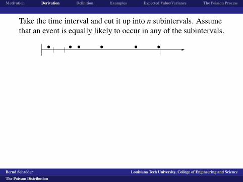
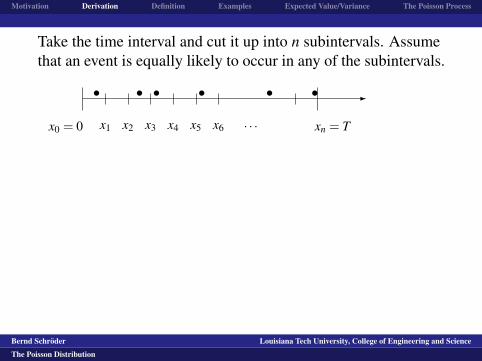
Take the time interval and cut it up into n subintervals.
Assumethat an event is equally likely to occur in any of the subintervals.
-s s s s s sx0 = 0 xn = Tx1 x2 x3 x4 x5 x6 · · · xn−1
That means there is a λ > 0 so that the probability that an event
occurs in a given time interval is p =λ
n. We keep this λ
independent of the number of subintervals. That way, if wedouble the number of intervals, for each interval the probabilityof an event occurring is divided by 2.
These assumptions are realistic for hits on web pages, forcustomer support calls received, for radioactive particlesregistered.
Bernd Schroder Louisiana Tech University, College of Engineering and Science
The Poisson Distribution

logo1
Motivation Derivation Definition Examples Expected Value/Variance The Poisson Process
Take the time interval and cut it up into n subintervals. Assumethat an event is equally likely to occur in any of the subintervals.
-
s s s s s sx0 = 0 xn = Tx1 x2 x3 x4 x5 x6 · · · xn−1
That means there is a λ > 0 so that the probability that an event
occurs in a given time interval is p =λ
n. We keep this λ
independent of the number of subintervals. That way, if wedouble the number of intervals, for each interval the probabilityof an event occurring is divided by 2.
These assumptions are realistic for hits on web pages, forcustomer support calls received, for radioactive particlesregistered.
Bernd Schroder Louisiana Tech University, College of Engineering and Science
The Poisson Distribution

logo1
Motivation Derivation Definition Examples Expected Value/Variance The Poisson Process
Take the time interval and cut it up into n subintervals. Assumethat an event is equally likely to occur in any of the subintervals.
-s
s s s s sx0 = 0 xn = Tx1 x2 x3 x4 x5 x6 · · · xn−1
That means there is a λ > 0 so that the probability that an event
occurs in a given time interval is p =λ
n. We keep this λ
independent of the number of subintervals. That way, if wedouble the number of intervals, for each interval the probabilityof an event occurring is divided by 2.
These assumptions are realistic for hits on web pages, forcustomer support calls received, for radioactive particlesregistered.
Bernd Schroder Louisiana Tech University, College of Engineering and Science
The Poisson Distribution

logo1
Motivation Derivation Definition Examples Expected Value/Variance The Poisson Process
Take the time interval and cut it up into n subintervals. Assumethat an event is equally likely to occur in any of the subintervals.
-s s
s s s sx0 = 0 xn = Tx1 x2 x3 x4 x5 x6 · · · xn−1
That means there is a λ > 0 so that the probability that an event
occurs in a given time interval is p =λ
n. We keep this λ
independent of the number of subintervals. That way, if wedouble the number of intervals, for each interval the probabilityof an event occurring is divided by 2.
These assumptions are realistic for hits on web pages, forcustomer support calls received, for radioactive particlesregistered.
Bernd Schroder Louisiana Tech University, College of Engineering and Science
The Poisson Distribution

logo1
Motivation Derivation Definition Examples Expected Value/Variance The Poisson Process
Take the time interval and cut it up into n subintervals. Assumethat an event is equally likely to occur in any of the subintervals.
-s s s
s s sx0 = 0 xn = Tx1 x2 x3 x4 x5 x6 · · · xn−1
That means there is a λ > 0 so that the probability that an event
occurs in a given time interval is p =λ
n. We keep this λ
independent of the number of subintervals. That way, if wedouble the number of intervals, for each interval the probabilityof an event occurring is divided by 2.
These assumptions are realistic for hits on web pages, forcustomer support calls received, for radioactive particlesregistered.
Bernd Schroder Louisiana Tech University, College of Engineering and Science
The Poisson Distribution

logo1
Motivation Derivation Definition Examples Expected Value/Variance The Poisson Process
Take the time interval and cut it up into n subintervals. Assumethat an event is equally likely to occur in any of the subintervals.
-s s s s
s sx0 = 0 xn = Tx1 x2 x3 x4 x5 x6 · · · xn−1
That means there is a λ > 0 so that the probability that an event
occurs in a given time interval is p =λ
n. We keep this λ
independent of the number of subintervals. That way, if wedouble the number of intervals, for each interval the probabilityof an event occurring is divided by 2.
These assumptions are realistic for hits on web pages, forcustomer support calls received, for radioactive particlesregistered.
Bernd Schroder Louisiana Tech University, College of Engineering and Science
The Poisson Distribution

logo1
Motivation Derivation Definition Examples Expected Value/Variance The Poisson Process
Take the time interval and cut it up into n subintervals. Assumethat an event is equally likely to occur in any of the subintervals.
-s s s s s
sx0 = 0 xn = Tx1 x2 x3 x4 x5 x6 · · · xn−1
That means there is a λ > 0 so that the probability that an event
occurs in a given time interval is p =λ
n. We keep this λ
independent of the number of subintervals. That way, if wedouble the number of intervals, for each interval the probabilityof an event occurring is divided by 2.
These assumptions are realistic for hits on web pages, forcustomer support calls received, for radioactive particlesregistered.
Bernd Schroder Louisiana Tech University, College of Engineering and Science
The Poisson Distribution

logo1
Motivation Derivation Definition Examples Expected Value/Variance The Poisson Process
Take the time interval and cut it up into n subintervals. Assumethat an event is equally likely to occur in any of the subintervals.
-s s s s s s
x0 = 0 xn = Tx1 x2 x3 x4 x5 x6 · · · xn−1
That means there is a λ > 0 so that the probability that an event
occurs in a given time interval is p =λ
n. We keep this λ
independent of the number of subintervals. That way, if wedouble the number of intervals, for each interval the probabilityof an event occurring is divided by 2.
These assumptions are realistic for hits on web pages, forcustomer support calls received, for radioactive particlesregistered.
Bernd Schroder Louisiana Tech University, College of Engineering and Science
The Poisson Distribution

logo1
Motivation Derivation Definition Examples Expected Value/Variance The Poisson Process
Take the time interval and cut it up into n subintervals. Assumethat an event is equally likely to occur in any of the subintervals.
-s s s s s sx0 = 0
xn = Tx1 x2 x3 x4 x5 x6 · · · xn−1
That means there is a λ > 0 so that the probability that an event
occurs in a given time interval is p =λ
n. We keep this λ
independent of the number of subintervals. That way, if wedouble the number of intervals, for each interval the probabilityof an event occurring is divided by 2.
These assumptions are realistic for hits on web pages, forcustomer support calls received, for radioactive particlesregistered.
Bernd Schroder Louisiana Tech University, College of Engineering and Science
The Poisson Distribution

logo1
Motivation Derivation Definition Examples Expected Value/Variance The Poisson Process
Take the time interval and cut it up into n subintervals. Assumethat an event is equally likely to occur in any of the subintervals.
-s s s s s sx0 = 0 xn = T
x1 x2 x3 x4 x5 x6 · · · xn−1
That means there is a λ > 0 so that the probability that an event
occurs in a given time interval is p =λ
n. We keep this λ
independent of the number of subintervals. That way, if wedouble the number of intervals, for each interval the probabilityof an event occurring is divided by 2.
These assumptions are realistic for hits on web pages, forcustomer support calls received, for radioactive particlesregistered.
Bernd Schroder Louisiana Tech University, College of Engineering and Science
The Poisson Distribution

logo1
Motivation Derivation Definition Examples Expected Value/Variance The Poisson Process
Take the time interval and cut it up into n subintervals. Assumethat an event is equally likely to occur in any of the subintervals.
-s s s s s sx0 = 0 xn = Tx1
x2 x3 x4 x5 x6 · · · xn−1
That means there is a λ > 0 so that the probability that an event
occurs in a given time interval is p =λ
n. We keep this λ
independent of the number of subintervals. That way, if wedouble the number of intervals, for each interval the probabilityof an event occurring is divided by 2.
These assumptions are realistic for hits on web pages, forcustomer support calls received, for radioactive particlesregistered.
Bernd Schroder Louisiana Tech University, College of Engineering and Science
The Poisson Distribution

logo1
Motivation Derivation Definition Examples Expected Value/Variance The Poisson Process
Take the time interval and cut it up into n subintervals. Assumethat an event is equally likely to occur in any of the subintervals.
-s s s s s sx0 = 0 xn = Tx1 x2
x3 x4 x5 x6 · · · xn−1
That means there is a λ > 0 so that the probability that an event
occurs in a given time interval is p =λ
n. We keep this λ
independent of the number of subintervals. That way, if wedouble the number of intervals, for each interval the probabilityof an event occurring is divided by 2.
These assumptions are realistic for hits on web pages, forcustomer support calls received, for radioactive particlesregistered.
Bernd Schroder Louisiana Tech University, College of Engineering and Science
The Poisson Distribution

logo1
Motivation Derivation Definition Examples Expected Value/Variance The Poisson Process
Take the time interval and cut it up into n subintervals. Assumethat an event is equally likely to occur in any of the subintervals.
-s s s s s sx0 = 0 xn = Tx1 x2 x3
x4 x5 x6 · · · xn−1
That means there is a λ > 0 so that the probability that an event
occurs in a given time interval is p =λ
n. We keep this λ
independent of the number of subintervals. That way, if wedouble the number of intervals, for each interval the probabilityof an event occurring is divided by 2.
These assumptions are realistic for hits on web pages, forcustomer support calls received, for radioactive particlesregistered.
Bernd Schroder Louisiana Tech University, College of Engineering and Science
The Poisson Distribution

logo1
Motivation Derivation Definition Examples Expected Value/Variance The Poisson Process
Take the time interval and cut it up into n subintervals. Assumethat an event is equally likely to occur in any of the subintervals.
-s s s s s sx0 = 0 xn = Tx1 x2 x3 x4
x5 x6 · · · xn−1
That means there is a λ > 0 so that the probability that an event
occurs in a given time interval is p =λ
n. We keep this λ
independent of the number of subintervals. That way, if wedouble the number of intervals, for each interval the probabilityof an event occurring is divided by 2.
These assumptions are realistic for hits on web pages, forcustomer support calls received, for radioactive particlesregistered.
Bernd Schroder Louisiana Tech University, College of Engineering and Science
The Poisson Distribution

logo1
Motivation Derivation Definition Examples Expected Value/Variance The Poisson Process
Take the time interval and cut it up into n subintervals. Assumethat an event is equally likely to occur in any of the subintervals.
-s s s s s sx0 = 0 xn = Tx1 x2 x3 x4 x5
x6 · · · xn−1
That means there is a λ > 0 so that the probability that an event
occurs in a given time interval is p =λ
n. We keep this λ
independent of the number of subintervals. That way, if wedouble the number of intervals, for each interval the probabilityof an event occurring is divided by 2.
These assumptions are realistic for hits on web pages, forcustomer support calls received, for radioactive particlesregistered.
Bernd Schroder Louisiana Tech University, College of Engineering and Science
The Poisson Distribution

logo1
Motivation Derivation Definition Examples Expected Value/Variance The Poisson Process
Take the time interval and cut it up into n subintervals. Assumethat an event is equally likely to occur in any of the subintervals.
-s s s s s sx0 = 0 xn = Tx1 x2 x3 x4 x5 x6
· · · xn−1
That means there is a λ > 0 so that the probability that an event
occurs in a given time interval is p =λ
n. We keep this λ
independent of the number of subintervals. That way, if wedouble the number of intervals, for each interval the probabilityof an event occurring is divided by 2.
These assumptions are realistic for hits on web pages, forcustomer support calls received, for radioactive particlesregistered.
Bernd Schroder Louisiana Tech University, College of Engineering and Science
The Poisson Distribution
logo1
Motivation Derivation Definition Examples Expected Value/Variance The Poisson Process
Take the time interval and cut it up into n subintervals. Assumethat an event is equally likely to occur in any of the subintervals.
-s s s s s sx0 = 0 xn = Tx1 x2 x3 x4 x5 x6 · · ·
xn−1
That means there is a λ > 0 so that the probability that an event
occurs in a given time interval is p =λ
n. We keep this λ
independent of the number of subintervals. That way, if wedouble the number of intervals, for each interval the probabilityof an event occurring is divided by 2.
These assumptions are realistic for hits on web pages, forcustomer support calls received, for radioactive particlesregistered.
Bernd Schroder Louisiana Tech University, College of Engineering and Science
The Poisson Distribution

logo1
Motivation Derivation Definition Examples Expected Value/Variance The Poisson Process
Take the time interval and cut it up into n subintervals. Assumethat an event is equally likely to occur in any of the subintervals.
-s s s s s sx0 = 0 xn = Tx1 x2 x3 x4 x5 x6 · · · xn−1
That means there is a λ > 0 so that the probability that an event
occurs in a given time interval is p =λ
n. We keep this λ
independent of the number of subintervals. That way, if wedouble the number of intervals, for each interval the probabilityof an event occurring is divided by 2.
These assumptions are realistic for hits on web pages, forcustomer support calls received, for radioactive particlesregistered.
Bernd Schroder Louisiana Tech University, College of Engineering and Science
The Poisson Distribution

logo1
Motivation Derivation Definition Examples Expected Value/Variance The Poisson Process
Take the time interval and cut it up into n subintervals. Assumethat an event is equally likely to occur in any of the subintervals.
-s s s s s sx0 = 0 xn = Tx1 x2 x3 x4 x5 x6 · · · xn−1
That means there is a λ > 0 so that the probability that an event
occurs in a given time interval is p =λ
n.
We keep this λ
independent of the number of subintervals. That way, if wedouble the number of intervals, for each interval the probabilityof an event occurring is divided by 2.
These assumptions are realistic for hits on web pages, forcustomer support calls received, for radioactive particlesregistered.
Bernd Schroder Louisiana Tech University, College of Engineering and Science
The Poisson Distribution

logo1
Motivation Derivation Definition Examples Expected Value/Variance The Poisson Process
Take the time interval and cut it up into n subintervals. Assumethat an event is equally likely to occur in any of the subintervals.
-s s s s s sx0 = 0 xn = Tx1 x2 x3 x4 x5 x6 · · · xn−1
That means there is a λ > 0 so that the probability that an event
occurs in a given time interval is p =λ
n. We keep this λ
independent of the number of subintervals.
That way, if wedouble the number of intervals, for each interval the probabilityof an event occurring is divided by 2.
These assumptions are realistic for hits on web pages, forcustomer support calls received, for radioactive particlesregistered.
Bernd Schroder Louisiana Tech University, College of Engineering and Science
The Poisson Distribution

logo1
Motivation Derivation Definition Examples Expected Value/Variance The Poisson Process
Take the time interval and cut it up into n subintervals. Assumethat an event is equally likely to occur in any of the subintervals.
-s s s s s sx0 = 0 xn = Tx1 x2 x3 x4 x5 x6 · · · xn−1
That means there is a λ > 0 so that the probability that an event
occurs in a given time interval is p =λ
n. We keep this λ
independent of the number of subintervals. That way, if wedouble the number of intervals, for each interval the probabilityof an event occurring is divided by 2.
These assumptions are realistic for hits on web pages, forcustomer support calls received, for radioactive particlesregistered.
Bernd Schroder Louisiana Tech University, College of Engineering and Science
The Poisson Distribution

logo1
Motivation Derivation Definition Examples Expected Value/Variance The Poisson Process
Take the time interval and cut it up into n subintervals. Assumethat an event is equally likely to occur in any of the subintervals.
-s s s s s sx0 = 0 xn = Tx1 x2 x3 x4 x5 x6 · · · xn−1
That means there is a λ > 0 so that the probability that an event
occurs in a given time interval is p =λ
n. We keep this λ
independent of the number of subintervals. That way, if wedouble the number of intervals, for each interval the probabilityof an event occurring is divided by 2.
These assumptions are realistic
for hits on web pages, forcustomer support calls received, for radioactive particlesregistered.
Bernd Schroder Louisiana Tech University, College of Engineering and Science
The Poisson Distribution

logo1
Motivation Derivation Definition Examples Expected Value/Variance The Poisson Process
Take the time interval and cut it up into n subintervals. Assumethat an event is equally likely to occur in any of the subintervals.
-s s s s s sx0 = 0 xn = Tx1 x2 x3 x4 x5 x6 · · · xn−1
That means there is a λ > 0 so that the probability that an event
occurs in a given time interval is p =λ
n. We keep this λ
independent of the number of subintervals. That way, if wedouble the number of intervals, for each interval the probabilityof an event occurring is divided by 2.
These assumptions are realistic for hits on web pages
, forcustomer support calls received, for radioactive particlesregistered.
Bernd Schroder Louisiana Tech University, College of Engineering and Science
The Poisson Distribution

logo1
Motivation Derivation Definition Examples Expected Value/Variance The Poisson Process
Take the time interval and cut it up into n subintervals. Assumethat an event is equally likely to occur in any of the subintervals.
-s s s s s sx0 = 0 xn = Tx1 x2 x3 x4 x5 x6 · · · xn−1
That means there is a λ > 0 so that the probability that an event
occurs in a given time interval is p =λ
n. We keep this λ
independent of the number of subintervals. That way, if wedouble the number of intervals, for each interval the probabilityof an event occurring is divided by 2.
These assumptions are realistic for hits on web pages, forcustomer support calls received
, for radioactive particlesregistered.
Bernd Schroder Louisiana Tech University, College of Engineering and Science
The Poisson Distribution

logo1
Motivation Derivation Definition Examples Expected Value/Variance The Poisson Process
Take the time interval and cut it up into n subintervals. Assumethat an event is equally likely to occur in any of the subintervals.
-s s s s s sx0 = 0 xn = Tx1 x2 x3 x4 x5 x6 · · · xn−1
That means there is a λ > 0 so that the probability that an event
occurs in a given time interval is p =λ
n. We keep this λ
independent of the number of subintervals. That way, if wedouble the number of intervals, for each interval the probabilityof an event occurring is divided by 2.
These assumptions are realistic for hits on web pages, forcustomer support calls received, for radioactive particlesregistered.
Bernd Schroder Louisiana Tech University, College of Engineering and Science
The Poisson Distribution

logo1
Motivation Derivation Definition Examples Expected Value/Variance The Poisson Process
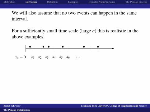
We will also assume that no two events can happen in the sameinterval.
For a sufficiently small time scale (large n) this is realistic in theabove examples.
-s s s s ssx0 = 0 x1 x2 x3 x4 x5 x6 · · · xn−1 xn = T
Plus, we could argue that within time intervals of a certainlength only one event can be registered.
Bernd Schroder Louisiana Tech University, College of Engineering and Science
The Poisson Distribution

logo1
Motivation Derivation Definition Examples Expected Value/Variance The Poisson Process
We will also assume that no two events can happen in the sameinterval.
For a sufficiently small time scale (large n) this is realistic in theabove examples.
-s s s s ss
x0 = 0 x1 x2 x3 x4 x5 x6 · · · xn−1 xn = T
Plus, we could argue that within time intervals of a certainlength only one event can be registered.
Bernd Schroder Louisiana Tech University, College of Engineering and Science
The Poisson Distribution

logo1
Motivation Derivation Definition Examples Expected Value/Variance The Poisson Process
We will also assume that no two events can happen in the sameinterval.
For a sufficiently small time scale (large n) this is realistic in theabove examples.
-s s s s ssx0 = 0
x1 x2 x3 x4 x5 x6 · · · xn−1 xn = T
Plus, we could argue that within time intervals of a certainlength only one event can be registered.
Bernd Schroder Louisiana Tech University, College of Engineering and Science
The Poisson Distribution

logo1
Motivation Derivation Definition Examples Expected Value/Variance The Poisson Process
We will also assume that no two events can happen in the sameinterval.
For a sufficiently small time scale (large n) this is realistic in theabove examples.
-s s s s ssx0 = 0 x1
x2 x3 x4 x5 x6 · · · xn−1 xn = T
Plus, we could argue that within time intervals of a certainlength only one event can be registered.
Bernd Schroder Louisiana Tech University, College of Engineering and Science
The Poisson Distribution

logo1
Motivation Derivation Definition Examples Expected Value/Variance The Poisson Process
We will also assume that no two events can happen in the sameinterval.
For a sufficiently small time scale (large n) this is realistic in theabove examples.
-s s s s ssx0 = 0 x1 x2
x3 x4 x5 x6 · · · xn−1 xn = T
Plus, we could argue that within time intervals of a certainlength only one event can be registered.
Bernd Schroder Louisiana Tech University, College of Engineering and Science
The Poisson Distribution

logo1
Motivation Derivation Definition Examples Expected Value/Variance The Poisson Process
We will also assume that no two events can happen in the sameinterval.
For a sufficiently small time scale (large n) this is realistic in theabove examples.
-s s s s ssx0 = 0 x1 x2 x3
x4 x5 x6 · · · xn−1 xn = T
Plus, we could argue that within time intervals of a certainlength only one event can be registered.
Bernd Schroder Louisiana Tech University, College of Engineering and Science
The Poisson Distribution

logo1
Motivation Derivation Definition Examples Expected Value/Variance The Poisson Process
We will also assume that no two events can happen in the sameinterval.
For a sufficiently small time scale (large n) this is realistic in theabove examples.
-s s s s ssx0 = 0 x1 x2 x3 x4
x5 x6 · · · xn−1 xn = T
Plus, we could argue that within time intervals of a certainlength only one event can be registered.
Bernd Schroder Louisiana Tech University, College of Engineering and Science
The Poisson Distribution

logo1
Motivation Derivation Definition Examples Expected Value/Variance The Poisson Process
We will also assume that no two events can happen in the sameinterval.
For a sufficiently small time scale (large n) this is realistic in theabove examples.
-s s s s ssx0 = 0 x1 x2 x3 x4 x5
x6 · · · xn−1 xn = T
Plus, we could argue that within time intervals of a certainlength only one event can be registered.
Bernd Schroder Louisiana Tech University, College of Engineering and Science
The Poisson Distribution

logo1
Motivation Derivation Definition Examples Expected Value/Variance The Poisson Process
We will also assume that no two events can happen in the sameinterval.
For a sufficiently small time scale (large n) this is realistic in theabove examples.
-s s s s ssx0 = 0 x1 x2 x3 x4 x5 x6
· · · xn−1 xn = T
Plus, we could argue that within time intervals of a certainlength only one event can be registered.
Bernd Schroder Louisiana Tech University, College of Engineering and Science
The Poisson Distribution
logo1
Motivation Derivation Definition Examples Expected Value/Variance The Poisson Process
We will also assume that no two events can happen in the sameinterval.
For a sufficiently small time scale (large n) this is realistic in theabove examples.
-s s s s ssx0 = 0 x1 x2 x3 x4 x5 x6 · · ·
xn−1 xn = T
Plus, we could argue that within time intervals of a certainlength only one event can be registered.
Bernd Schroder Louisiana Tech University, College of Engineering and Science
The Poisson Distribution

logo1
Motivation Derivation Definition Examples Expected Value/Variance The Poisson Process
We will also assume that no two events can happen in the sameinterval.
For a sufficiently small time scale (large n) this is realistic in theabove examples.
-s s s s ssx0 = 0 x1 x2 x3 x4 x5 x6 · · · xn−1
xn = T
Plus, we could argue that within time intervals of a certainlength only one event can be registered.
Bernd Schroder Louisiana Tech University, College of Engineering and Science
The Poisson Distribution

logo1
Motivation Derivation Definition Examples Expected Value/Variance The Poisson Process
We will also assume that no two events can happen in the sameinterval.
For a sufficiently small time scale (large n) this is realistic in theabove examples.
-s s s s ssx0 = 0 x1 x2 x3 x4 x5 x6 · · · xn−1 xn = T
Plus, we could argue that within time intervals of a certainlength only one event can be registered.
Bernd Schroder Louisiana Tech University, College of Engineering and Science
The Poisson Distribution

logo1
Motivation Derivation Definition Examples Expected Value/Variance The Poisson Process
We will also assume that no two events can happen in the sameinterval.
For a sufficiently small time scale (large n) this is realistic in theabove examples.
-s s s s ssx0 = 0 x1 x2 x3 x4 x5 x6 · · · xn−1 xn = T
Plus, we could argue that within time intervals of a certainlength only one event can be registered.
Bernd Schroder Louisiana Tech University, College of Engineering and Science
The Poisson Distribution

logo1
Motivation Derivation Definition Examples Expected Value/Variance The Poisson Process
Under the assumptions that
the interval we investigate has nsubintervals so that the probability an event occurs in a
subinterval is p =λ
nand that at most one event occurs in each
subinterval, the probability that x events occur overall is givenby the binomial distribution.
b(x;n,p) =(
nx
)px(1−p)n−x =
n!(n− x)!x!
λ x
nx
(1− λ
n
)n−x
=n!
(n− x)!nxλ x
x!
((1− λ
n
)n) n−xn
n→∞−→ 1 · λx
x!· e−λ
(We let n→ ∞ because cutting up the original time interval wasjust a way to get the model.)
Bernd Schroder Louisiana Tech University, College of Engineering and Science
The Poisson Distribution
logo1
Motivation Derivation Definition Examples Expected Value/Variance The Poisson Process
Under the assumptions that the interval we investigate has nsubintervals
so that the probability an event occurs in a
subinterval is p =λ
nand that at most one event occurs in each
subinterval, the probability that x events occur overall is givenby the binomial distribution.
b(x;n,p) =(
nx
)px(1−p)n−x =
n!(n− x)!x!
λ x
nx
(1− λ
n
)n−x
=n!
(n− x)!nxλ x
x!
((1− λ
n
)n) n−xn
n→∞−→ 1 · λx
x!· e−λ
(We let n→ ∞ because cutting up the original time interval wasjust a way to get the model.)
Bernd Schroder Louisiana Tech University, College of Engineering and Science
The Poisson Distribution

logo1
Motivation Derivation Definition Examples Expected Value/Variance The Poisson Process
Under the assumptions that the interval we investigate has nsubintervals so that the probability an event occurs in a
subinterval is p =λ
n
and that at most one event occurs in eachsubinterval, the probability that x events occur overall is givenby the binomial distribution.
b(x;n,p) =(
nx
)px(1−p)n−x =
n!(n− x)!x!
λ x
nx
(1− λ
n
)n−x
=n!
(n− x)!nxλ x
x!
((1− λ
n
)n) n−xn
n→∞−→ 1 · λx
x!· e−λ
(We let n→ ∞ because cutting up the original time interval wasjust a way to get the model.)
Bernd Schroder Louisiana Tech University, College of Engineering and Science
The Poisson Distribution

logo1
Motivation Derivation Definition Examples Expected Value/Variance The Poisson Process
Under the assumptions that the interval we investigate has nsubintervals so that the probability an event occurs in a
subinterval is p =λ
nand that at most one event occurs in each
subinterval,
the probability that x events occur overall is givenby the binomial distribution.
b(x;n,p) =(
nx
)px(1−p)n−x =
n!(n− x)!x!
λ x
nx
(1− λ
n
)n−x
=n!
(n− x)!nxλ x
x!
((1− λ
n
)n) n−xn
n→∞−→ 1 · λx
x!· e−λ
(We let n→ ∞ because cutting up the original time interval wasjust a way to get the model.)
Bernd Schroder Louisiana Tech University, College of Engineering and Science
The Poisson Distribution

logo1
Motivation Derivation Definition Examples Expected Value/Variance The Poisson Process
Under the assumptions that the interval we investigate has nsubintervals so that the probability an event occurs in a
subinterval is p =λ
nand that at most one event occurs in each
subinterval, the probability that x events occur overall is givenby the binomial distribution.
b(x;n,p) =(
nx
)px(1−p)n−x =
n!(n− x)!x!
λ x
nx
(1− λ
n
)n−x
=n!
(n− x)!nxλ x
x!
((1− λ
n
)n) n−xn
n→∞−→ 1 · λx
x!· e−λ
(We let n→ ∞ because cutting up the original time interval wasjust a way to get the model.)
Bernd Schroder Louisiana Tech University, College of Engineering and Science
The Poisson Distribution

logo1
Motivation Derivation Definition Examples Expected Value/Variance The Poisson Process
Under the assumptions that the interval we investigate has nsubintervals so that the probability an event occurs in a
subinterval is p =λ
nand that at most one event occurs in each
subinterval, the probability that x events occur overall is givenby the binomial distribution.
b(x;n,p)
=(
nx
)px(1−p)n−x =
n!(n− x)!x!
λ x
nx
(1− λ
n
)n−x
=n!
(n− x)!nxλ x
x!
((1− λ
n
)n) n−xn
n→∞−→ 1 · λx
x!· e−λ
(We let n→ ∞ because cutting up the original time interval wasjust a way to get the model.)
Bernd Schroder Louisiana Tech University, College of Engineering and Science
The Poisson Distribution

logo1
Motivation Derivation Definition Examples Expected Value/Variance The Poisson Process
Under the assumptions that the interval we investigate has nsubintervals so that the probability an event occurs in a
subinterval is p =λ
nand that at most one event occurs in each
subinterval, the probability that x events occur overall is givenby the binomial distribution.
b(x;n,p) =(
nx
)px(1−p)n−x
=n!
(n− x)!x!λ x
nx
(1− λ
n
)n−x
=n!
(n− x)!nxλ x
x!
((1− λ
n
)n) n−xn
n→∞−→ 1 · λx
x!· e−λ
(We let n→ ∞ because cutting up the original time interval wasjust a way to get the model.)
Bernd Schroder Louisiana Tech University, College of Engineering and Science
The Poisson Distribution

logo1
Motivation Derivation Definition Examples Expected Value/Variance The Poisson Process
Under the assumptions that the interval we investigate has nsubintervals so that the probability an event occurs in a
subinterval is p =λ
nand that at most one event occurs in each
subinterval, the probability that x events occur overall is givenby the binomial distribution.
b(x;n,p) =(
nx
)px(1−p)n−x =
n!(n− x)!x!
λ x
nx
(1− λ
n
)n−x
=n!
(n− x)!nxλ x
x!
((1− λ
n
)n) n−xn
n→∞−→ 1 · λx
x!· e−λ
(We let n→ ∞ because cutting up the original time interval wasjust a way to get the model.)
Bernd Schroder Louisiana Tech University, College of Engineering and Science
The Poisson Distribution

logo1
Motivation Derivation Definition Examples Expected Value/Variance The Poisson Process
Under the assumptions that the interval we investigate has nsubintervals so that the probability an event occurs in a
subinterval is p =λ
nand that at most one event occurs in each
subinterval, the probability that x events occur overall is givenby the binomial distribution.
b(x;n,p) =(
nx
)px(1−p)n−x =
n!(n− x)!x!
λ x
nx
(1− λ
n
)n−x
=n!
(n− x)!nxλ x
x!
((1− λ
n
)n) n−xn
n→∞−→ 1
· λx
x!· e−λ
(We let n→ ∞ because cutting up the original time interval wasjust a way to get the model.)
Bernd Schroder Louisiana Tech University, College of Engineering and Science
The Poisson Distribution

logo1
Motivation Derivation Definition Examples Expected Value/Variance The Poisson Process
Under the assumptions that the interval we investigate has nsubintervals so that the probability an event occurs in a
subinterval is p =λ
nand that at most one event occurs in each
subinterval, the probability that x events occur overall is givenby the binomial distribution.
b(x;n,p) =(
nx
)px(1−p)n−x =
n!(n− x)!x!
λ x
nx
(1− λ
n
)n−x
=n!
(n− x)!nxλ x
x!
((1− λ
n
)n) n−xn
n→∞−→ 1 · λx
x!
· e−λ
(We let n→ ∞ because cutting up the original time interval wasjust a way to get the model.)
Bernd Schroder Louisiana Tech University, College of Engineering and Science
The Poisson Distribution

logo1
Motivation Derivation Definition Examples Expected Value/Variance The Poisson Process
Under the assumptions that the interval we investigate has nsubintervals so that the probability an event occurs in a
subinterval is p =λ
nand that at most one event occurs in each
subinterval, the probability that x events occur overall is givenby the binomial distribution.
b(x;n,p) =(
nx
)px(1−p)n−x =
n!(n− x)!x!
λ x
nx
(1− λ
n
)n−x
=n!
(n− x)!nxλ x
x!
((1− λ
n
)n) n−xn
n→∞−→ 1 · λx
x!· e−λ
(We let n→ ∞ because cutting up the original time interval wasjust a way to get the model.)
Bernd Schroder Louisiana Tech University, College of Engineering and Science
The Poisson Distribution

logo1
Motivation Derivation Definition Examples Expected Value/Variance The Poisson Process
Under the assumptions that the interval we investigate has nsubintervals so that the probability an event occurs in a
subinterval is p =λ
nand that at most one event occurs in each
subinterval, the probability that x events occur overall is givenby the binomial distribution.
b(x;n,p) =(
nx
)px(1−p)n−x =
n!(n− x)!x!
λ x
nx
(1− λ
n
)n−x
=n!
(n− x)!nxλ x
x!
((1− λ
n
)n) n−xn
n→∞−→ 1 · λx
x!· e−λ
(We let n→ ∞ because cutting up the original time interval wasjust a way to get the model.)
Bernd Schroder Louisiana Tech University, College of Engineering and Science
The Poisson Distribution

logo1
Motivation Derivation Definition Examples Expected Value/Variance The Poisson Process
Definition.
A random variable is said to have a Poissondistribution with parameter λ > 0 if and only if its probability
mass function is p(x;λ ) =e−λ λ x
x!
This really is a probability mass function, because of the series
representation of the exponential function: eλ =∞
∑x=0
λ x
x!.
Bernd Schroder Louisiana Tech University, College of Engineering and Science
The Poisson Distribution

logo1
Motivation Derivation Definition Examples Expected Value/Variance The Poisson Process
Definition. A random variable is said to have a Poissondistribution with parameter λ > 0
if and only if its probability
mass function is p(x;λ ) =e−λ λ x
x!
This really is a probability mass function, because of the series
representation of the exponential function: eλ =∞
∑x=0
λ x
x!.
Bernd Schroder Louisiana Tech University, College of Engineering and Science
The Poisson Distribution

logo1
Motivation Derivation Definition Examples Expected Value/Variance The Poisson Process
Definition. A random variable is said to have a Poissondistribution with parameter λ > 0 if and only if its probability
mass function is p(x;λ ) =e−λ λ x
x!
This really is a probability mass function, because of the series
representation of the exponential function
: eλ =∞
∑x=0
λ x
x!.
Bernd Schroder Louisiana Tech University, College of Engineering and Science
The Poisson Distribution

logo1
Motivation Derivation Definition Examples Expected Value/Variance The Poisson Process
Definition. A random variable is said to have a Poissondistribution with parameter λ > 0 if and only if its probability
mass function is p(x;λ ) =e−λ λ x
x!
This really is a probability mass function, because of the series
representation of the exponential function: eλ =∞
∑x=0
λ x
x!.
Bernd Schroder Louisiana Tech University, College of Engineering and Science
The Poisson Distribution

logo1
Motivation Derivation Definition Examples Expected Value/Variance The Poisson Process
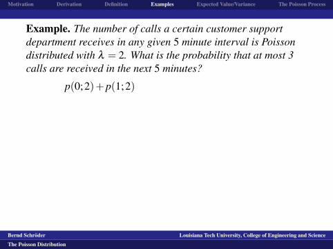
Example.
The number of calls a certain customer supportdepartment receives in any given 5 minute interval is Poissondistributed with λ = 2. What is the probability that at most 3calls are received in the next 5 minutes?
p(0;2)+p(1;2)+p(2;2)+p(3;2) = 0.857
(Used a Poisson distribution table to look up p(x≤ 3;2), whichis just a value of the cumulative distribution function.)
Bernd Schroder Louisiana Tech University, College of Engineering and Science
The Poisson Distribution

logo1
Motivation Derivation Definition Examples Expected Value/Variance The Poisson Process
Example. The number of calls a certain customer supportdepartment receives in any given 5 minute interval is Poissondistributed with λ = 2.
What is the probability that at most 3calls are received in the next 5 minutes?
p(0;2)+p(1;2)+p(2;2)+p(3;2) = 0.857
(Used a Poisson distribution table to look up p(x≤ 3;2), whichis just a value of the cumulative distribution function.)
Bernd Schroder Louisiana Tech University, College of Engineering and Science
The Poisson Distribution

logo1
Motivation Derivation Definition Examples Expected Value/Variance The Poisson Process
Example. The number of calls a certain customer supportdepartment receives in any given 5 minute interval is Poissondistributed with λ = 2. What is the probability that at most 3calls are received in the next 5 minutes?
p(0;2)
+p(1;2)+p(2;2)+p(3;2) = 0.857
(Used a Poisson distribution table to look up p(x≤ 3;2), whichis just a value of the cumulative distribution function.)
Bernd Schroder Louisiana Tech University, College of Engineering and Science
The Poisson Distribution
logo1
Motivation Derivation Definition Examples Expected Value/Variance The Poisson Process
Example. The number of calls a certain customer supportdepartment receives in any given 5 minute interval is Poissondistributed with λ = 2. What is the probability that at most 3calls are received in the next 5 minutes?
p(0;2)+p(1;2)
+p(2;2)+p(3;2) = 0.857
(Used a Poisson distribution table to look up p(x≤ 3;2), whichis just a value of the cumulative distribution function.)
Bernd Schroder Louisiana Tech University, College of Engineering and Science
The Poisson Distribution

logo1
Motivation Derivation Definition Examples Expected Value/Variance The Poisson Process
Example. The number of calls a certain customer supportdepartment receives in any given 5 minute interval is Poissondistributed with λ = 2. What is the probability that at most 3calls are received in the next 5 minutes?
p(0;2)+p(1;2)+p(2;2)
+p(3;2) = 0.857
(Used a Poisson distribution table to look up p(x≤ 3;2), whichis just a value of the cumulative distribution function.)
Bernd Schroder Louisiana Tech University, College of Engineering and Science
The Poisson Distribution

logo1
Motivation Derivation Definition Examples Expected Value/Variance The Poisson Process
Example. The number of calls a certain customer supportdepartment receives in any given 5 minute interval is Poissondistributed with λ = 2. What is the probability that at most 3calls are received in the next 5 minutes?
p(0;2)+p(1;2)+p(2;2)+p(3;2)
= 0.857
(Used a Poisson distribution table to look up p(x≤ 3;2), whichis just a value of the cumulative distribution function.)
Bernd Schroder Louisiana Tech University, College of Engineering and Science
The Poisson Distribution

logo1
Motivation Derivation Definition Examples Expected Value/Variance The Poisson Process
Example. The number of calls a certain customer supportdepartment receives in any given 5 minute interval is Poissondistributed with λ = 2. What is the probability that at most 3calls are received in the next 5 minutes?
p(0;2)+p(1;2)+p(2;2)+p(3;2) = 0.857
(Used a Poisson distribution table to look up p(x≤ 3;2), whichis just a value of the cumulative distribution function.)
Bernd Schroder Louisiana Tech University, College of Engineering and Science
The Poisson Distribution

logo1
Motivation Derivation Definition Examples Expected Value/Variance The Poisson Process
Example. The number of calls a certain customer supportdepartment receives in any given 5 minute interval is Poissondistributed with λ = 2. What is the probability that at most 3calls are received in the next 5 minutes?
p(0;2)+p(1;2)+p(2;2)+p(3;2) = 0.857
(Used a Poisson distribution table to look up p(x≤ 3;2), whichis just a value of the cumulative distribution function.)
Bernd Schroder Louisiana Tech University, College of Engineering and Science
The Poisson Distribution

logo1
Motivation Derivation Definition Examples Expected Value/Variance The Poisson Process
For large values of n, the Poisson distribution can be used toapproximate binomial probabilities.
Example. Suppose the probability of a missing page in anindividual book a certain manufacturer makes is 0.1. What isthe probability that a batch of 200 books has at most 10 bookswith a page missing?Using a Poisson distribution, we have thatλ = np = 200 ·0.1 = 20.Now from a Poisson distribution table, p(x≤ 10;20)≈ 0.011.
With a CAS we obtain B(10;200,0.1)≈ 0.008.
Bernd Schroder Louisiana Tech University, College of Engineering and Science
The Poisson Distribution

logo1
Motivation Derivation Definition Examples Expected Value/Variance The Poisson Process
For large values of n, the Poisson distribution can be used toapproximate binomial probabilities.
Example.
Suppose the probability of a missing page in anindividual book a certain manufacturer makes is 0.1. What isthe probability that a batch of 200 books has at most 10 bookswith a page missing?Using a Poisson distribution, we have thatλ = np = 200 ·0.1 = 20.Now from a Poisson distribution table, p(x≤ 10;20)≈ 0.011.
With a CAS we obtain B(10;200,0.1)≈ 0.008.
Bernd Schroder Louisiana Tech University, College of Engineering and Science
The Poisson Distribution
logo1
Motivation Derivation Definition Examples Expected Value/Variance The Poisson Process
For large values of n, the Poisson distribution can be used toapproximate binomial probabilities.
Example. Suppose the probability of a missing page in anindividual book a certain manufacturer makes is 0.1.
What isthe probability that a batch of 200 books has at most 10 bookswith a page missing?Using a Poisson distribution, we have thatλ = np = 200 ·0.1 = 20.Now from a Poisson distribution table, p(x≤ 10;20)≈ 0.011.
With a CAS we obtain B(10;200,0.1)≈ 0.008.
Bernd Schroder Louisiana Tech University, College of Engineering and Science
The Poisson Distribution

logo1
Motivation Derivation Definition Examples Expected Value/Variance The Poisson Process
For large values of n, the Poisson distribution can be used toapproximate binomial probabilities.
Example. Suppose the probability of a missing page in anindividual book a certain manufacturer makes is 0.1. What isthe probability that a batch of 200 books has at most 10 bookswith a page missing?
Using a Poisson distribution, we have thatλ = np = 200 ·0.1 = 20.Now from a Poisson distribution table, p(x≤ 10;20)≈ 0.011.
With a CAS we obtain B(10;200,0.1)≈ 0.008.
Bernd Schroder Louisiana Tech University, College of Engineering and Science
The Poisson Distribution

logo1
Motivation Derivation Definition Examples Expected Value/Variance The Poisson Process
For large values of n, the Poisson distribution can be used toapproximate binomial probabilities.
Example. Suppose the probability of a missing page in anindividual book a certain manufacturer makes is 0.1. What isthe probability that a batch of 200 books has at most 10 bookswith a page missing?Using a Poisson distribution, we have that
λ = np = 200 ·0.1 = 20.Now from a Poisson distribution table, p(x≤ 10;20)≈ 0.011.
With a CAS we obtain B(10;200,0.1)≈ 0.008.
Bernd Schroder Louisiana Tech University, College of Engineering and Science
The Poisson Distribution
logo1
Motivation Derivation Definition Examples Expected Value/Variance The Poisson Process
For large values of n, the Poisson distribution can be used toapproximate binomial probabilities.
Example. Suppose the probability of a missing page in anindividual book a certain manufacturer makes is 0.1. What isthe probability that a batch of 200 books has at most 10 bookswith a page missing?Using a Poisson distribution, we have thatλ
= np = 200 ·0.1 = 20.Now from a Poisson distribution table, p(x≤ 10;20)≈ 0.011.
With a CAS we obtain B(10;200,0.1)≈ 0.008.
Bernd Schroder Louisiana Tech University, College of Engineering and Science
The Poisson Distribution

logo1
Motivation Derivation Definition Examples Expected Value/Variance The Poisson Process
For large values of n, the Poisson distribution can be used toapproximate binomial probabilities.
Example. Suppose the probability of a missing page in anindividual book a certain manufacturer makes is 0.1. What isthe probability that a batch of 200 books has at most 10 bookswith a page missing?Using a Poisson distribution, we have thatλ = np
= 200 ·0.1 = 20.Now from a Poisson distribution table, p(x≤ 10;20)≈ 0.011.
With a CAS we obtain B(10;200,0.1)≈ 0.008.
Bernd Schroder Louisiana Tech University, College of Engineering and Science
The Poisson Distribution
logo1
Motivation Derivation Definition Examples Expected Value/Variance The Poisson Process
For large values of n, the Poisson distribution can be used toapproximate binomial probabilities.
Example. Suppose the probability of a missing page in anindividual book a certain manufacturer makes is 0.1. What isthe probability that a batch of 200 books has at most 10 bookswith a page missing?Using a Poisson distribution, we have thatλ = np = 200 ·0.1
= 20.Now from a Poisson distribution table, p(x≤ 10;20)≈ 0.011.
With a CAS we obtain B(10;200,0.1)≈ 0.008.
Bernd Schroder Louisiana Tech University, College of Engineering and Science
The Poisson Distribution

logo1
Motivation Derivation Definition Examples Expected Value/Variance The Poisson Process
For large values of n, the Poisson distribution can be used toapproximate binomial probabilities.
Example. Suppose the probability of a missing page in anindividual book a certain manufacturer makes is 0.1. What isthe probability that a batch of 200 books has at most 10 bookswith a page missing?Using a Poisson distribution, we have thatλ = np = 200 ·0.1 = 20.
Now from a Poisson distribution table, p(x≤ 10;20)≈ 0.011.
With a CAS we obtain B(10;200,0.1)≈ 0.008.
Bernd Schroder Louisiana Tech University, College of Engineering and Science
The Poisson Distribution

logo1
Motivation Derivation Definition Examples Expected Value/Variance The Poisson Process
For large values of n, the Poisson distribution can be used toapproximate binomial probabilities.
Example. Suppose the probability of a missing page in anindividual book a certain manufacturer makes is 0.1. What isthe probability that a batch of 200 books has at most 10 bookswith a page missing?Using a Poisson distribution, we have thatλ = np = 200 ·0.1 = 20.Now from a Poisson distribution table, p(x≤ 10;20)≈ 0.011.
With a CAS we obtain B(10;200,0.1)≈ 0.008.
Bernd Schroder Louisiana Tech University, College of Engineering and Science
The Poisson Distribution

logo1
Motivation Derivation Definition Examples Expected Value/Variance The Poisson Process
For large values of n, the Poisson distribution can be used toapproximate binomial probabilities.
Example. Suppose the probability of a missing page in anindividual book a certain manufacturer makes is 0.1. What isthe probability that a batch of 200 books has at most 10 bookswith a page missing?Using a Poisson distribution, we have thatλ = np = 200 ·0.1 = 20.Now from a Poisson distribution table, p(x≤ 10;20)≈ 0.011.
With a CAS we obtain B(10;200,0.1)≈ 0.008.
Bernd Schroder Louisiana Tech University, College of Engineering and Science
The Poisson Distribution

logo1
Motivation Derivation Definition Examples Expected Value/Variance The Poisson Process
Theorem.
Let X be a Poisson distributed random variable.Then E(X) = λ and V(X) = λ .
Proof.
E(X) =∞
∑x=0
xe−λ λ x
x!=
∞
∑x=1
e−λ λ x
(x−1)!
= λe−λ∞
∑x=1
λ x−1
(x−1)!= λe−λ
∞
∑j=0
λ j
j!
= λe−λ eλ = λ
Bernd Schroder Louisiana Tech University, College of Engineering and Science
The Poisson Distribution

logo1
Motivation Derivation Definition Examples Expected Value/Variance The Poisson Process
Theorem. Let X be a Poisson distributed random variable.
Then E(X) = λ and V(X) = λ .
Proof.
E(X) =∞
∑x=0
xe−λ λ x
x!=
∞
∑x=1
e−λ λ x
(x−1)!
= λe−λ∞
∑x=1
λ x−1
(x−1)!= λe−λ
∞
∑j=0
λ j
j!
= λe−λ eλ = λ
Bernd Schroder Louisiana Tech University, College of Engineering and Science
The Poisson Distribution

logo1
Motivation Derivation Definition Examples Expected Value/Variance The Poisson Process
Theorem. Let X be a Poisson distributed random variable.Then E(X) = λ and V(X) = λ .
Proof.
E(X)
=∞
∑x=0
xe−λ λ x
x!=
∞
∑x=1
e−λ λ x
(x−1)!
= λe−λ∞
∑x=1
λ x−1
(x−1)!= λe−λ
∞
∑j=0
λ j
j!
= λe−λ eλ = λ
Bernd Schroder Louisiana Tech University, College of Engineering and Science
The Poisson Distribution

logo1
Motivation Derivation Definition Examples Expected Value/Variance The Poisson Process
Theorem. Let X be a Poisson distributed random variable.Then E(X) = λ and V(X) = λ .
Proof.
E(X) =∞
∑x=0
xe−λ λ x
x!
=∞
∑x=1
e−λ λ x
(x−1)!
= λe−λ∞
∑x=1
λ x−1
(x−1)!= λe−λ
∞
∑j=0
λ j
j!
= λe−λ eλ = λ
Bernd Schroder Louisiana Tech University, College of Engineering and Science
The Poisson Distribution

logo1
Motivation Derivation Definition Examples Expected Value/Variance The Poisson Process
Theorem. Let X be a Poisson distributed random variable.Then E(X) = λ and V(X) = λ .
Proof.
E(X) =∞
∑x=0
xe−λ λ x
x!=
∞
∑x=1
e−λ λ x
(x−1)!
= λe−λ∞
∑x=1
λ x−1
(x−1)!= λe−λ
∞
∑j=0
λ j
j!
= λe−λ eλ = λ
Bernd Schroder Louisiana Tech University, College of Engineering and Science
The Poisson Distribution

logo1
Motivation Derivation Definition Examples Expected Value/Variance The Poisson Process
Theorem. Let X be a Poisson distributed random variable.Then E(X) = λ and V(X) = λ .
Proof.
E(X) =∞
∑x=0
xe−λ λ x
x!=
∞
∑x=1
e−λ λ x
(x−1)!
= λe−λ∞
∑x=1
λ x−1
(x−1)!
= λe−λ∞
∑j=0
λ j
j!
= λe−λ eλ = λ
Bernd Schroder Louisiana Tech University, College of Engineering and Science
The Poisson Distribution

logo1
Motivation Derivation Definition Examples Expected Value/Variance The Poisson Process
Theorem. Let X be a Poisson distributed random variable.Then E(X) = λ and V(X) = λ .
Proof.
E(X) =∞
∑x=0
xe−λ λ x
x!=
∞
∑x=1
e−λ λ x
(x−1)!
= λe−λ∞
∑x=1
λ x−1
(x−1)!= λe−λ
∞
∑j=0
λ j
j!
= λe−λ eλ = λ
Bernd Schroder Louisiana Tech University, College of Engineering and Science
The Poisson Distribution

logo1
Motivation Derivation Definition Examples Expected Value/Variance The Poisson Process
Theorem. Let X be a Poisson distributed random variable.Then E(X) = λ and V(X) = λ .
Proof.
E(X) =∞
∑x=0
xe−λ λ x
x!=
∞
∑x=1
e−λ λ x
(x−1)!
= λe−λ∞
∑x=1
λ x−1
(x−1)!= λe−λ
∞
∑j=0
λ j
j!
= λe−λ eλ
= λ
Bernd Schroder Louisiana Tech University, College of Engineering and Science
The Poisson Distribution

logo1
Motivation Derivation Definition Examples Expected Value/Variance The Poisson Process
Theorem. Let X be a Poisson distributed random variable.Then E(X) = λ and V(X) = λ .
Proof.
E(X) =∞
∑x=0
xe−λ λ x
x!=
∞
∑x=1
e−λ λ x
(x−1)!
= λe−λ∞
∑x=1
λ x−1
(x−1)!= λe−λ
∞
∑j=0
λ j
j!
= λe−λ eλ = λ
Bernd Schroder Louisiana Tech University, College of Engineering and Science
The Poisson Distribution

logo1
Motivation Derivation Definition Examples Expected Value/Variance The Poisson Process
E(
X2)
=∞
∑x=0
x2 e−λ λ x
x!=
∞
∑x=0
x(x−1)e−λ λ x
x!+
∞
∑x=0
xe−λ λ x
x!
=∞
∑x=2
x(x−1)e−λ λ x
x!+λ = e−λ
λ2
∞
∑x=2
λ x−2
(x−2)!+λ
= e−λλ
2∞
∑k=0
λ k
k!+λ = e−λ
λ2eλ +λ
= λ2 +λ
V(X) = E(
X2)−E (X)2 = λ
2 +λ −λ2 = λ
Bernd Schroder Louisiana Tech University, College of Engineering and Science
The Poisson Distribution

logo1
Motivation Derivation Definition Examples Expected Value/Variance The Poisson Process
E(
X2)
=∞
∑x=0
x2 e−λ λ x
x!
=∞
∑x=0
x(x−1)e−λ λ x
x!+
∞
∑x=0
xe−λ λ x
x!
=∞
∑x=2
x(x−1)e−λ λ x
x!+λ = e−λ
λ2
∞
∑x=2
λ x−2
(x−2)!+λ
= e−λλ
2∞
∑k=0
λ k
k!+λ = e−λ
λ2eλ +λ
= λ2 +λ
V(X) = E(
X2)−E (X)2 = λ
2 +λ −λ2 = λ
Bernd Schroder Louisiana Tech University, College of Engineering and Science
The Poisson Distribution

logo1
Motivation Derivation Definition Examples Expected Value/Variance The Poisson Process
E(
X2)
=∞
∑x=0
x2 e−λ λ x
x!=
∞
∑x=0
x(x−1)e−λ λ x
x!+
∞
∑x=0
xe−λ λ x
x!
=∞
∑x=2
x(x−1)e−λ λ x
x!+λ = e−λ
λ2
∞
∑x=2
λ x−2
(x−2)!+λ
= e−λλ
2∞
∑k=0
λ k
k!+λ = e−λ
λ2eλ +λ
= λ2 +λ
V(X) = E(
X2)−E (X)2 = λ
2 +λ −λ2 = λ
Bernd Schroder Louisiana Tech University, College of Engineering and Science
The Poisson Distribution

logo1
Motivation Derivation Definition Examples Expected Value/Variance The Poisson Process
E(
X2)
=∞
∑x=0
x2 e−λ λ x
x!=
∞
∑x=0
x(x−1)e−λ λ x
x!+
∞
∑x=0
xe−λ λ x
x!
=∞
∑x=2
x(x−1)e−λ λ x
x!+λ
= e−λλ
2∞
∑x=2
λ x−2
(x−2)!+λ
= e−λλ
2∞
∑k=0
λ k
k!+λ = e−λ
λ2eλ +λ
= λ2 +λ
V(X) = E(
X2)−E (X)2 = λ
2 +λ −λ2 = λ
Bernd Schroder Louisiana Tech University, College of Engineering and Science
The Poisson Distribution

logo1
Motivation Derivation Definition Examples Expected Value/Variance The Poisson Process
E(
X2)
=∞
∑x=0
x2 e−λ λ x
x!=
∞
∑x=0
x(x−1)e−λ λ x
x!+
∞
∑x=0
xe−λ λ x
x!
=∞
∑x=2
x(x−1)e−λ λ x
x!+λ = e−λ
λ2
∞
∑x=2
λ x−2
(x−2)!+λ
= e−λλ
2∞
∑k=0
λ k
k!+λ = e−λ
λ2eλ +λ
= λ2 +λ
V(X) = E(
X2)−E (X)2 = λ
2 +λ −λ2 = λ
Bernd Schroder Louisiana Tech University, College of Engineering and Science
The Poisson Distribution
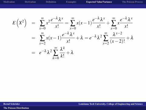
logo1
Motivation Derivation Definition Examples Expected Value/Variance The Poisson Process
E(
X2)
=∞
∑x=0
x2 e−λ λ x
x!=
∞
∑x=0
x(x−1)e−λ λ x
x!+
∞
∑x=0
xe−λ λ x
x!
=∞
∑x=2
x(x−1)e−λ λ x
x!+λ = e−λ
λ2
∞
∑x=2
λ x−2
(x−2)!+λ
= e−λλ
2∞
∑k=0
λ k
k!+λ
= e−λλ
2eλ +λ
= λ2 +λ
V(X) = E(
X2)−E (X)2 = λ
2 +λ −λ2 = λ
Bernd Schroder Louisiana Tech University, College of Engineering and Science
The Poisson Distribution

logo1
Motivation Derivation Definition Examples Expected Value/Variance The Poisson Process
E(
X2)
=∞
∑x=0
x2 e−λ λ x
x!=
∞
∑x=0
x(x−1)e−λ λ x
x!+
∞
∑x=0
xe−λ λ x
x!
=∞
∑x=2
x(x−1)e−λ λ x
x!+λ = e−λ
λ2
∞
∑x=2
λ x−2
(x−2)!+λ
= e−λλ
2∞
∑k=0
λ k
k!+λ = e−λ
λ2eλ +λ
= λ2 +λ
V(X) = E(
X2)−E (X)2 = λ
2 +λ −λ2 = λ
Bernd Schroder Louisiana Tech University, College of Engineering and Science
The Poisson Distribution

logo1
Motivation Derivation Definition Examples Expected Value/Variance The Poisson Process
E(
X2)
=∞
∑x=0
x2 e−λ λ x
x!=
∞
∑x=0
x(x−1)e−λ λ x
x!+
∞
∑x=0
xe−λ λ x
x!
=∞
∑x=2
x(x−1)e−λ λ x
x!+λ = e−λ
λ2
∞
∑x=2
λ x−2
(x−2)!+λ
= e−λλ
2∞
∑k=0
λ k
k!+λ = e−λ
λ2eλ +λ
= λ2 +λ
V(X)
= E(
X2)−E (X)2 = λ
2 +λ −λ2 = λ
Bernd Schroder Louisiana Tech University, College of Engineering and Science
The Poisson Distribution

logo1
Motivation Derivation Definition Examples Expected Value/Variance The Poisson Process
E(
X2)
=∞
∑x=0
x2 e−λ λ x
x!=
∞
∑x=0
x(x−1)e−λ λ x
x!+
∞
∑x=0
xe−λ λ x
x!
=∞
∑x=2
x(x−1)e−λ λ x
x!+λ = e−λ
λ2
∞
∑x=2
λ x−2
(x−2)!+λ
= e−λλ
2∞
∑k=0
λ k
k!+λ = e−λ
λ2eλ +λ
= λ2 +λ
V(X) = E(
X2)−E (X)2
= λ2 +λ −λ
2 = λ
Bernd Schroder Louisiana Tech University, College of Engineering and Science
The Poisson Distribution

logo1
Motivation Derivation Definition Examples Expected Value/Variance The Poisson Process
E(
X2)
=∞
∑x=0
x2 e−λ λ x
x!=
∞
∑x=0
x(x−1)e−λ λ x
x!+
∞
∑x=0
xe−λ λ x
x!
=∞
∑x=2
x(x−1)e−λ λ x
x!+λ = e−λ
λ2
∞
∑x=2
λ x−2
(x−2)!+λ
= e−λλ
2∞
∑k=0
λ k
k!+λ = e−λ
λ2eλ +λ
= λ2 +λ
V(X) = E(
X2)−E (X)2 = λ
2 +λ −λ2
= λ
Bernd Schroder Louisiana Tech University, College of Engineering and Science
The Poisson Distribution

logo1
Motivation Derivation Definition Examples Expected Value/Variance The Poisson Process
E(
X2)
=∞
∑x=0
x2 e−λ λ x
x!=
∞
∑x=0
x(x−1)e−λ λ x
x!+
∞
∑x=0
xe−λ λ x
x!
=∞
∑x=2
x(x−1)e−λ λ x
x!+λ = e−λ
λ2
∞
∑x=2
λ x−2
(x−2)!+λ
= e−λλ
2∞
∑k=0
λ k
k!+λ = e−λ
λ2eλ +λ
= λ2 +λ
V(X) = E(
X2)−E (X)2 = λ
2 +λ −λ2 = λ
Bernd Schroder Louisiana Tech University, College of Engineering and Science
The Poisson Distribution

logo1
Motivation Derivation Definition Examples Expected Value/Variance The Poisson Process
E(
X2)
=∞
∑x=0
x2 e−λ λ x
x!=
∞
∑x=0
x(x−1)e−λ λ x
x!+
∞
∑x=0
xe−λ λ x
x!
=∞
∑x=2
x(x−1)e−λ λ x
x!+λ = e−λ
λ2
∞
∑x=2
λ x−2
(x−2)!+λ
= e−λλ
2∞
∑k=0
λ k
k!+λ = e−λ
λ2eλ +λ
= λ2 +λ
V(X) = E(
X2)−E (X)2 = λ
2 +λ −λ2 = λ
Bernd Schroder Louisiana Tech University, College of Engineering and Science
The Poisson Distribution

logo1
Motivation Derivation Definition Examples Expected Value/Variance The Poisson Process
Extending to Arbitrary Intervals
A Poisson process is a stochastic process with the followingproperties.
1. There is an α > 0 so that for a short interval ∆t theprobability of one event is α∆t +o(∆t).
2. The probability of more than one event is o(∆t).3. The number of events in an interval ∆t is independent of
the number received in other intervals.In a Poisson process with parameter α , the probability of kevents in an interval of length t is Poisson distributed withparameter λ = αt.
Pk(t) = e−αt (αt)k
k!.
Bernd Schroder Louisiana Tech University, College of Engineering and Science
The Poisson Distribution

logo1
Motivation Derivation Definition Examples Expected Value/Variance The Poisson Process
Extending to Arbitrary IntervalsA Poisson process is a stochastic process with the followingproperties.
1. There is an α > 0 so that for a short interval ∆t theprobability of one event is α∆t +o(∆t).
2. The probability of more than one event is o(∆t).
3. The number of events in an interval ∆t is independent ofthe number received in other intervals.
In a Poisson process with parameter α , the probability of kevents in an interval of length t is Poisson distributed withparameter λ = αt.
Pk(t) = e−αt (αt)k
k!.
Bernd Schroder Louisiana Tech University, College of Engineering and Science
The Poisson Distribution

logo1
Motivation Derivation Definition Examples Expected Value/Variance The Poisson Process
Extending to Arbitrary IntervalsA Poisson process is a stochastic process with the followingproperties.
1. There is an α > 0 so that for a short interval ∆t theprobability of one event is α∆t +o(∆t).
2. The probability of more than one event is o(∆t).3. The number of events in an interval ∆t is independent of
the number received in other intervals.
In a Poisson process with parameter α , the probability of kevents in an interval of length t is Poisson distributed withparameter λ = αt.
Pk(t) = e−αt (αt)k
k!.
Bernd Schroder Louisiana Tech University, College of Engineering and Science
The Poisson Distribution

logo1
Motivation Derivation Definition Examples Expected Value/Variance The Poisson Process
Extending to Arbitrary IntervalsA Poisson process is a stochastic process with the followingproperties.
1. There is an α > 0 so that for a short interval ∆t theprobability of one event is α∆t +o(∆t).
2. The probability of more than one event is o(∆t).3. The number of events in an interval ∆t is independent of
the number received in other intervals.In a Poisson process with parameter α , the probability of kevents in an interval of length t is Poisson distributed withparameter λ = αt.
Pk(t) = e−αt (αt)k
k!.
Bernd Schroder Louisiana Tech University, College of Engineering and Science
The Poisson Distribution

logo1
Motivation Derivation Definition Examples Expected Value/Variance The Poisson Process
Extending to Arbitrary IntervalsA Poisson process is a stochastic process with the followingproperties.
1. There is an α > 0 so that for a short interval ∆t theprobability of one event is α∆t +o(∆t).
2. The probability of more than one event is o(∆t).3. The number of events in an interval ∆t is independent of
the number received in other intervals.In a Poisson process with parameter α , the probability of kevents in an interval of length t is Poisson distributed withparameter λ = αt.
Pk(t) = e−αt (αt)k
k!.
Bernd Schroder Louisiana Tech University, College of Engineering and Science
The Poisson Distribution

logo1
Motivation Derivation Definition Examples Expected Value/Variance The Poisson Process
Example.
Particles are registered by a Geiger counter at anaverage rate of 2 particles per second. Find the probability that4 or more particles are registered in a given second.
The probability of registering a particle in a time interval isproportional to the length ∆t of the interval, so it’s α∆t. Forreally short time intervals, the probability of registering twoparticles is zero (particles will arrive at different times, countermust “reset”). The number of particles received in a timeinterval does not depend on the past. So this is a Poissonprocess with α = 2 and interval length t = 1.
P(X ≥ 4) = 1−P0(1)−P1(1)−P2(1)−P3(1)
= 1− e−2 20
0!− e−2 21
1!− e−2 22
2!− e−2 23
3!≈ 0.1429
Bernd Schroder Louisiana Tech University, College of Engineering and Science
The Poisson Distribution

logo1
Motivation Derivation Definition Examples Expected Value/Variance The Poisson Process
Example. Particles are registered by a Geiger counter at anaverage rate of 2 particles per second.
Find the probability that4 or more particles are registered in a given second.
The probability of registering a particle in a time interval isproportional to the length ∆t of the interval, so it’s α∆t. Forreally short time intervals, the probability of registering twoparticles is zero (particles will arrive at different times, countermust “reset”). The number of particles received in a timeinterval does not depend on the past. So this is a Poissonprocess with α = 2 and interval length t = 1.
P(X ≥ 4) = 1−P0(1)−P1(1)−P2(1)−P3(1)
= 1− e−2 20
0!− e−2 21
1!− e−2 22
2!− e−2 23
3!≈ 0.1429
Bernd Schroder Louisiana Tech University, College of Engineering and Science
The Poisson Distribution

logo1
Motivation Derivation Definition Examples Expected Value/Variance The Poisson Process
Example. Particles are registered by a Geiger counter at anaverage rate of 2 particles per second. Find the probability that4 or more particles are registered in a given second.
The probability of registering a particle in a time interval isproportional to the length ∆t of the interval
, so it’s α∆t. Forreally short time intervals, the probability of registering twoparticles is zero (particles will arrive at different times, countermust “reset”). The number of particles received in a timeinterval does not depend on the past. So this is a Poissonprocess with α = 2 and interval length t = 1.
P(X ≥ 4) = 1−P0(1)−P1(1)−P2(1)−P3(1)
= 1− e−2 20
0!− e−2 21
1!− e−2 22
2!− e−2 23
3!≈ 0.1429
Bernd Schroder Louisiana Tech University, College of Engineering and Science
The Poisson Distribution
logo1
Motivation Derivation Definition Examples Expected Value/Variance The Poisson Process
Example. Particles are registered by a Geiger counter at anaverage rate of 2 particles per second. Find the probability that4 or more particles are registered in a given second.
The probability of registering a particle in a time interval isproportional to the length ∆t of the interval, so it’s α∆t.
Forreally short time intervals, the probability of registering twoparticles is zero (particles will arrive at different times, countermust “reset”). The number of particles received in a timeinterval does not depend on the past. So this is a Poissonprocess with α = 2 and interval length t = 1.
P(X ≥ 4) = 1−P0(1)−P1(1)−P2(1)−P3(1)
= 1− e−2 20
0!− e−2 21
1!− e−2 22
2!− e−2 23
3!≈ 0.1429
Bernd Schroder Louisiana Tech University, College of Engineering and Science
The Poisson Distribution

logo1
Motivation Derivation Definition Examples Expected Value/Variance The Poisson Process
Example. Particles are registered by a Geiger counter at anaverage rate of 2 particles per second. Find the probability that4 or more particles are registered in a given second.
The probability of registering a particle in a time interval isproportional to the length ∆t of the interval, so it’s α∆t. Forreally short time intervals, the probability of registering twoparticles is zero
(particles will arrive at different times, countermust “reset”). The number of particles received in a timeinterval does not depend on the past. So this is a Poissonprocess with α = 2 and interval length t = 1.
P(X ≥ 4) = 1−P0(1)−P1(1)−P2(1)−P3(1)
= 1− e−2 20
0!− e−2 21
1!− e−2 22
2!− e−2 23
3!≈ 0.1429
Bernd Schroder Louisiana Tech University, College of Engineering and Science
The Poisson Distribution

logo1
Motivation Derivation Definition Examples Expected Value/Variance The Poisson Process
Example. Particles are registered by a Geiger counter at anaverage rate of 2 particles per second. Find the probability that4 or more particles are registered in a given second.
The probability of registering a particle in a time interval isproportional to the length ∆t of the interval, so it’s α∆t. Forreally short time intervals, the probability of registering twoparticles is zero (particles will arrive at different times
, countermust “reset”). The number of particles received in a timeinterval does not depend on the past. So this is a Poissonprocess with α = 2 and interval length t = 1.
P(X ≥ 4) = 1−P0(1)−P1(1)−P2(1)−P3(1)
= 1− e−2 20
0!− e−2 21
1!− e−2 22
2!− e−2 23
3!≈ 0.1429
Bernd Schroder Louisiana Tech University, College of Engineering and Science
The Poisson Distribution

logo1
Motivation Derivation Definition Examples Expected Value/Variance The Poisson Process
Example. Particles are registered by a Geiger counter at anaverage rate of 2 particles per second. Find the probability that4 or more particles are registered in a given second.
The probability of registering a particle in a time interval isproportional to the length ∆t of the interval, so it’s α∆t. Forreally short time intervals, the probability of registering twoparticles is zero (particles will arrive at different times, countermust “reset”).
The number of particles received in a timeinterval does not depend on the past. So this is a Poissonprocess with α = 2 and interval length t = 1.
P(X ≥ 4) = 1−P0(1)−P1(1)−P2(1)−P3(1)
= 1− e−2 20
0!− e−2 21
1!− e−2 22
2!− e−2 23
3!≈ 0.1429
Bernd Schroder Louisiana Tech University, College of Engineering and Science
The Poisson Distribution

logo1
Motivation Derivation Definition Examples Expected Value/Variance The Poisson Process
Example. Particles are registered by a Geiger counter at anaverage rate of 2 particles per second. Find the probability that4 or more particles are registered in a given second.
The probability of registering a particle in a time interval isproportional to the length ∆t of the interval, so it’s α∆t. Forreally short time intervals, the probability of registering twoparticles is zero (particles will arrive at different times, countermust “reset”). The number of particles received in a timeinterval does not depend on the past.
So this is a Poissonprocess with α = 2 and interval length t = 1.
P(X ≥ 4) = 1−P0(1)−P1(1)−P2(1)−P3(1)
= 1− e−2 20
0!− e−2 21
1!− e−2 22
2!− e−2 23
3!≈ 0.1429
Bernd Schroder Louisiana Tech University, College of Engineering and Science
The Poisson Distribution

logo1
Motivation Derivation Definition Examples Expected Value/Variance The Poisson Process
Example. Particles are registered by a Geiger counter at anaverage rate of 2 particles per second. Find the probability that4 or more particles are registered in a given second.
The probability of registering a particle in a time interval isproportional to the length ∆t of the interval, so it’s α∆t. Forreally short time intervals, the probability of registering twoparticles is zero (particles will arrive at different times, countermust “reset”). The number of particles received in a timeinterval does not depend on the past. So this is a Poissonprocess with α = 2 and interval length t = 1.
P(X ≥ 4) = 1−P0(1)−P1(1)−P2(1)−P3(1)
= 1− e−2 20
0!− e−2 21
1!− e−2 22
2!− e−2 23
3!≈ 0.1429
Bernd Schroder Louisiana Tech University, College of Engineering and Science
The Poisson Distribution

logo1
Motivation Derivation Definition Examples Expected Value/Variance The Poisson Process
Example. Particles are registered by a Geiger counter at anaverage rate of 2 particles per second. Find the probability that4 or more particles are registered in a given second.
The probability of registering a particle in a time interval isproportional to the length ∆t of the interval, so it’s α∆t. Forreally short time intervals, the probability of registering twoparticles is zero (particles will arrive at different times, countermust “reset”). The number of particles received in a timeinterval does not depend on the past. So this is a Poissonprocess with α = 2 and interval length t = 1.
P(X ≥ 4)
= 1−P0(1)−P1(1)−P2(1)−P3(1)
= 1− e−2 20
0!− e−2 21
1!− e−2 22
2!− e−2 23
3!≈ 0.1429
Bernd Schroder Louisiana Tech University, College of Engineering and Science
The Poisson Distribution

logo1
Motivation Derivation Definition Examples Expected Value/Variance The Poisson Process
Example. Particles are registered by a Geiger counter at anaverage rate of 2 particles per second. Find the probability that4 or more particles are registered in a given second.
The probability of registering a particle in a time interval isproportional to the length ∆t of the interval, so it’s α∆t. Forreally short time intervals, the probability of registering twoparticles is zero (particles will arrive at different times, countermust “reset”). The number of particles received in a timeinterval does not depend on the past. So this is a Poissonprocess with α = 2 and interval length t = 1.
P(X ≥ 4) = 1−P0(1)−P1(1)−P2(1)−P3(1)
= 1− e−2 20
0!− e−2 21
1!− e−2 22
2!− e−2 23
3!≈ 0.1429
Bernd Schroder Louisiana Tech University, College of Engineering and Science
The Poisson Distribution

logo1
Motivation Derivation Definition Examples Expected Value/Variance The Poisson Process
Example. Particles are registered by a Geiger counter at anaverage rate of 2 particles per second. Find the probability that4 or more particles are registered in a given second.
The probability of registering a particle in a time interval isproportional to the length ∆t of the interval, so it’s α∆t. Forreally short time intervals, the probability of registering twoparticles is zero (particles will arrive at different times, countermust “reset”). The number of particles received in a timeinterval does not depend on the past. So this is a Poissonprocess with α = 2 and interval length t = 1.
P(X ≥ 4) = 1−P0(1)−P1(1)−P2(1)−P3(1)
= 1− e−2 20
0!− e−2 21
1!− e−2 22
2!− e−2 23
3!
≈ 0.1429
Bernd Schroder Louisiana Tech University, College of Engineering and Science
The Poisson Distribution

logo1
Motivation Derivation Definition Examples Expected Value/Variance The Poisson Process
Example. Particles are registered by a Geiger counter at anaverage rate of 2 particles per second. Find the probability that4 or more particles are registered in a given second.
The probability of registering a particle in a time interval isproportional to the length ∆t of the interval, so it’s α∆t. Forreally short time intervals, the probability of registering twoparticles is zero (particles will arrive at different times, countermust “reset”). The number of particles received in a timeinterval does not depend on the past. So this is a Poissonprocess with α = 2 and interval length t = 1.
P(X ≥ 4) = 1−P0(1)−P1(1)−P2(1)−P3(1)
= 1− e−2 20
0!− e−2 21
1!− e−2 22
2!− e−2 23
3!≈ 0.1429
Bernd Schroder Louisiana Tech University, College of Engineering and Science
The Poisson Distribution

logo1
Motivation Derivation Definition Examples Expected Value/Variance The Poisson Process
Example.
Driving along a road, trees are seen to be kudzuinfested at an average rate of 3 trees per quarter mile. Find theprobability of encountering a kudzu free half mile stretch.
The probability of seeing an infested tree over a stretch of roadis proportional to the length ∆s of the stretch of road, so it’sα∆s. For really short lengths ∆s, the probability of two infestedtrees is 0. (How many trees are 1 in apart?) The number ofinfested trees on any given quarter mile is assumed to beindependent of the number on previous stretches of road. Sothis is a Poisson process with α = 12, if we use miles as theunit, and the length is s = 1/2.
P(X = 0) = P0
(12
)= e−12· 12
(12 · 1
2
)0
0!= e−6 ≈ 0.002479.
Bernd Schroder Louisiana Tech University, College of Engineering and Science
The Poisson Distribution

logo1
Motivation Derivation Definition Examples Expected Value/Variance The Poisson Process
Example. Driving along a road, trees are seen to be kudzuinfested at an average rate of 3 trees per quarter mile.
Find theprobability of encountering a kudzu free half mile stretch.
The probability of seeing an infested tree over a stretch of roadis proportional to the length ∆s of the stretch of road, so it’sα∆s. For really short lengths ∆s, the probability of two infestedtrees is 0. (How many trees are 1 in apart?) The number ofinfested trees on any given quarter mile is assumed to beindependent of the number on previous stretches of road. Sothis is a Poisson process with α = 12, if we use miles as theunit, and the length is s = 1/2.
P(X = 0) = P0
(12
)= e−12· 12
(12 · 1
2
)0
0!= e−6 ≈ 0.002479.
Bernd Schroder Louisiana Tech University, College of Engineering and Science
The Poisson Distribution

logo1
Motivation Derivation Definition Examples Expected Value/Variance The Poisson Process
Example. Driving along a road, trees are seen to be kudzuinfested at an average rate of 3 trees per quarter mile. Find theprobability of encountering a kudzu free half mile stretch.
The probability of seeing an infested tree over a stretch of roadis proportional to the length ∆s of the stretch of road
, so it’sα∆s. For really short lengths ∆s, the probability of two infestedtrees is 0. (How many trees are 1 in apart?) The number ofinfested trees on any given quarter mile is assumed to beindependent of the number on previous stretches of road. Sothis is a Poisson process with α = 12, if we use miles as theunit, and the length is s = 1/2.
P(X = 0) = P0
(12
)= e−12· 12
(12 · 1
2
)0
0!= e−6 ≈ 0.002479.
Bernd Schroder Louisiana Tech University, College of Engineering and Science
The Poisson Distribution

logo1
Motivation Derivation Definition Examples Expected Value/Variance The Poisson Process
Example. Driving along a road, trees are seen to be kudzuinfested at an average rate of 3 trees per quarter mile. Find theprobability of encountering a kudzu free half mile stretch.
The probability of seeing an infested tree over a stretch of roadis proportional to the length ∆s of the stretch of road, so it’sα∆s.
For really short lengths ∆s, the probability of two infestedtrees is 0. (How many trees are 1 in apart?) The number ofinfested trees on any given quarter mile is assumed to beindependent of the number on previous stretches of road. Sothis is a Poisson process with α = 12, if we use miles as theunit, and the length is s = 1/2.
P(X = 0) = P0
(12
)= e−12· 12
(12 · 1
2
)0
0!= e−6 ≈ 0.002479.
Bernd Schroder Louisiana Tech University, College of Engineering and Science
The Poisson Distribution

logo1
Motivation Derivation Definition Examples Expected Value/Variance The Poisson Process
Example. Driving along a road, trees are seen to be kudzuinfested at an average rate of 3 trees per quarter mile. Find theprobability of encountering a kudzu free half mile stretch.
The probability of seeing an infested tree over a stretch of roadis proportional to the length ∆s of the stretch of road, so it’sα∆s. For really short lengths ∆s, the probability of two infestedtrees is 0.
(How many trees are 1 in apart?) The number ofinfested trees on any given quarter mile is assumed to beindependent of the number on previous stretches of road. Sothis is a Poisson process with α = 12, if we use miles as theunit, and the length is s = 1/2.
P(X = 0) = P0
(12
)= e−12· 12
(12 · 1
2
)0
0!= e−6 ≈ 0.002479.
Bernd Schroder Louisiana Tech University, College of Engineering and Science
The Poisson Distribution

logo1
Motivation Derivation Definition Examples Expected Value/Variance The Poisson Process
Example. Driving along a road, trees are seen to be kudzuinfested at an average rate of 3 trees per quarter mile. Find theprobability of encountering a kudzu free half mile stretch.
The probability of seeing an infested tree over a stretch of roadis proportional to the length ∆s of the stretch of road, so it’sα∆s. For really short lengths ∆s, the probability of two infestedtrees is 0. (How many trees are 1 in apart?)
The number ofinfested trees on any given quarter mile is assumed to beindependent of the number on previous stretches of road. Sothis is a Poisson process with α = 12, if we use miles as theunit, and the length is s = 1/2.
P(X = 0) = P0
(12
)= e−12· 12
(12 · 1
2
)0
0!= e−6 ≈ 0.002479.
Bernd Schroder Louisiana Tech University, College of Engineering and Science
The Poisson Distribution

logo1
Motivation Derivation Definition Examples Expected Value/Variance The Poisson Process
Example. Driving along a road, trees are seen to be kudzuinfested at an average rate of 3 trees per quarter mile. Find theprobability of encountering a kudzu free half mile stretch.
The probability of seeing an infested tree over a stretch of roadis proportional to the length ∆s of the stretch of road, so it’sα∆s. For really short lengths ∆s, the probability of two infestedtrees is 0. (How many trees are 1 in apart?) The number ofinfested trees on any given quarter mile is assumed to beindependent of the number on previous stretches of road.
Sothis is a Poisson process with α = 12, if we use miles as theunit, and the length is s = 1/2.
P(X = 0) = P0
(12
)= e−12· 12
(12 · 1
2
)0
0!= e−6 ≈ 0.002479.
Bernd Schroder Louisiana Tech University, College of Engineering and Science
The Poisson Distribution

logo1
Motivation Derivation Definition Examples Expected Value/Variance The Poisson Process
Example. Driving along a road, trees are seen to be kudzuinfested at an average rate of 3 trees per quarter mile. Find theprobability of encountering a kudzu free half mile stretch.
The probability of seeing an infested tree over a stretch of roadis proportional to the length ∆s of the stretch of road, so it’sα∆s. For really short lengths ∆s, the probability of two infestedtrees is 0. (How many trees are 1 in apart?) The number ofinfested trees on any given quarter mile is assumed to beindependent of the number on previous stretches of road. Sothis is a Poisson process with α = 12, if we use miles as theunit
, and the length is s = 1/2.
P(X = 0) = P0
(12
)= e−12· 12
(12 · 1
2
)0
0!= e−6 ≈ 0.002479.
Bernd Schroder Louisiana Tech University, College of Engineering and Science
The Poisson Distribution

logo1
Motivation Derivation Definition Examples Expected Value/Variance The Poisson Process
Example. Driving along a road, trees are seen to be kudzuinfested at an average rate of 3 trees per quarter mile. Find theprobability of encountering a kudzu free half mile stretch.
The probability of seeing an infested tree over a stretch of roadis proportional to the length ∆s of the stretch of road, so it’sα∆s. For really short lengths ∆s, the probability of two infestedtrees is 0. (How many trees are 1 in apart?) The number ofinfested trees on any given quarter mile is assumed to beindependent of the number on previous stretches of road. Sothis is a Poisson process with α = 12, if we use miles as theunit, and the length is s = 1/2.
P(X = 0) = P0
(12
)= e−12· 12
(12 · 1
2
)0
0!= e−6 ≈ 0.002479.
Bernd Schroder Louisiana Tech University, College of Engineering and Science
The Poisson Distribution

logo1
Motivation Derivation Definition Examples Expected Value/Variance The Poisson Process
Example. Driving along a road, trees are seen to be kudzuinfested at an average rate of 3 trees per quarter mile. Find theprobability of encountering a kudzu free half mile stretch.
The probability of seeing an infested tree over a stretch of roadis proportional to the length ∆s of the stretch of road, so it’sα∆s. For really short lengths ∆s, the probability of two infestedtrees is 0. (How many trees are 1 in apart?) The number ofinfested trees on any given quarter mile is assumed to beindependent of the number on previous stretches of road. Sothis is a Poisson process with α = 12, if we use miles as theunit, and the length is s = 1/2.
P(X = 0)
= P0
(12
)= e−12· 12
(12 · 1
2
)0
0!= e−6 ≈ 0.002479.
Bernd Schroder Louisiana Tech University, College of Engineering and Science
The Poisson Distribution

logo1
Motivation Derivation Definition Examples Expected Value/Variance The Poisson Process
Example. Driving along a road, trees are seen to be kudzuinfested at an average rate of 3 trees per quarter mile. Find theprobability of encountering a kudzu free half mile stretch.
The probability of seeing an infested tree over a stretch of roadis proportional to the length ∆s of the stretch of road, so it’sα∆s. For really short lengths ∆s, the probability of two infestedtrees is 0. (How many trees are 1 in apart?) The number ofinfested trees on any given quarter mile is assumed to beindependent of the number on previous stretches of road. Sothis is a Poisson process with α = 12, if we use miles as theunit, and the length is s = 1/2.
P(X = 0) = P0
(12
)
= e−12· 12
(12 · 1
2
)0
0!= e−6 ≈ 0.002479.
Bernd Schroder Louisiana Tech University, College of Engineering and Science
The Poisson Distribution

logo1
Motivation Derivation Definition Examples Expected Value/Variance The Poisson Process
Example. Driving along a road, trees are seen to be kudzuinfested at an average rate of 3 trees per quarter mile. Find theprobability of encountering a kudzu free half mile stretch.
The probability of seeing an infested tree over a stretch of roadis proportional to the length ∆s of the stretch of road, so it’sα∆s. For really short lengths ∆s, the probability of two infestedtrees is 0. (How many trees are 1 in apart?) The number ofinfested trees on any given quarter mile is assumed to beindependent of the number on previous stretches of road. Sothis is a Poisson process with α = 12, if we use miles as theunit, and the length is s = 1/2.
P(X = 0) = P0
(12
)= e−12· 12
(12 · 1
2
)0
0!
= e−6 ≈ 0.002479.
Bernd Schroder Louisiana Tech University, College of Engineering and Science
The Poisson Distribution

logo1
Motivation Derivation Definition Examples Expected Value/Variance The Poisson Process
Example. Driving along a road, trees are seen to be kudzuinfested at an average rate of 3 trees per quarter mile. Find theprobability of encountering a kudzu free half mile stretch.
The probability of seeing an infested tree over a stretch of roadis proportional to the length ∆s of the stretch of road, so it’sα∆s. For really short lengths ∆s, the probability of two infestedtrees is 0. (How many trees are 1 in apart?) The number ofinfested trees on any given quarter mile is assumed to beindependent of the number on previous stretches of road. Sothis is a Poisson process with α = 12, if we use miles as theunit, and the length is s = 1/2.
P(X = 0) = P0
(12
)= e−12· 12
(12 · 1
2
)0
0!= e−6
≈ 0.002479.
Bernd Schroder Louisiana Tech University, College of Engineering and Science
The Poisson Distribution

logo1
Motivation Derivation Definition Examples Expected Value/Variance The Poisson Process
Example. Driving along a road, trees are seen to be kudzuinfested at an average rate of 3 trees per quarter mile. Find theprobability of encountering a kudzu free half mile stretch.
The probability of seeing an infested tree over a stretch of roadis proportional to the length ∆s of the stretch of road, so it’sα∆s. For really short lengths ∆s, the probability of two infestedtrees is 0. (How many trees are 1 in apart?) The number ofinfested trees on any given quarter mile is assumed to beindependent of the number on previous stretches of road. Sothis is a Poisson process with α = 12, if we use miles as theunit, and the length is s = 1/2.
P(X = 0) = P0
(12
)= e−12· 12
(12 · 1
2
)0
0!= e−6 ≈ 0.002479.
Bernd Schroder Louisiana Tech University, College of Engineering and Science
The Poisson Distribution