RNA Secondary Structures

Ivo L. Hofacker1 and Peter F. Stadler2,∗

1Institute for Theoretical Chemistry, University of Vienna,Wahringerstrasse 17, A-1090 Vienna, Austria2Bioinformatics Group, Department of Computer Science, and In-terdisciplinary Center for Bioinformatics, University of Leipzig,Hartelstrasse 16-18, D-04107 Leipzig, Germany.

Phone: ++49 341 97 16691, Fax: ++49 341 97 16709,

email: studla@bioinf.uni-leipzig.de

1

2

1. Secondary Structure Graphs

1.1. Introduction. The tendency of complementary strands of DNA to form doublehelices is well known since the work of Watson & Crick. Single stranded nucleic acidsequences will in general contain many complementary regions that have the potentialto form double helices when the molecule folds back onto itself. The resulting pat-tern of double helical stretches interspersed with loops is what is called the secondary

structure of an RNA or DNA. Secondary structure elements may in turn be arrangedin space to form 3-dimensional tertiary structure, leading to additional noncovalentinteractions, an example is shown in Fig. 1. Energetically, however, these tertiaryinteractions are weaker than secondary structure. As a consequence RNA foldingcan be regarded as a hierarchical process in which secondary structure forms beforetertiary structure [130, 129]. Since formation of tertiary structure usually does notinduce changes in secondary structure, the two processes can be described indepen-dently. Functional RNA molecules (tRNAs, ribosomal RNAs, etc., as opposed to purecoding sequences), usually have characteristic spatial structures — and therefore alsocharacteristic secondary structures — that are prerequisites for their function. As aconsequence, secondary structures are highly conserved in evolution for many classesof RNA molecules.

Both the experimental determination of full spatial RNA structures and computa-tional predictions of RNA 3D-structures are very hard tasks, arguable even harderthan the corresponding problems for proteins [62, 82]. Computational approachesto RNA tertiary structure thus have been successful only for selected cases, see nextchapter. RNA secondary structures, on the other hand, not only have a definite phys-ical meaning as folding intermediates and are useful tools in the interpretation RNAmolecules, but they give rise to efficient efficient computational techniques. Secondarystructure prediction and comparison, the focal topics of this chapter, have thereforebecome a routine tool in the analysis of RNA function.

RNA secondary structures consists of two distinct classes of residues: those thatare incorporated in double helical regions (so called stems), and those that are not

GCGGAUUU

AGCUC

AGDDG

G G AG A G C

GCCAGAC

UG A A

YAU

CUGGAGGU

CC U G U G

T P CG

AUCCACAG

AAUUCGC

A C C A

Anticodon

D-LoopT-Loop

Acceptor StemGCGGAUU

U

A

GCUCA

GD

DGG

GA G

AGCGCCAGAC

UG A A

YAU

CUGGA G

GUC

CUGUGTPC

GA U C

C A C A G A A U U C G C A C C A

Figure 1. Secondary and tertiary structure of yeast phenylalanine tRNA. Left: The clover-leaf shaped secondary structure consisting of four helices. The dotted blue lines mark evo-lutionary conserved tertiary contacts. Middle: Co-axial stacking results in two extendedhelices that form the L-shaped tertiary structure. Right: Tertiary structure taken fromPDB entry 4TRA. The color code (from red to blue) indicates the position along the chain.

3

ACACGACC

UC

AU

AU

AA

UCUUGGGAAUAUG

GC

CC

A U A A G U U U C U A C C C G G CA

AC

CG

UAAAUUGCCGGA

CU

AU

GC

AG

GGAAGUGA A

CAC

GA

CCUCAUAUA

AUCUUGGGAA

UA

U GGC C C AU

AAGUUUCUACC C G G C A AC

C GUA

AAUUGCCGG

A

CUAUGCAGG

GA

AGUGA

ACACGACCUCAUAUAAUCUUGGGAAUAUGGCCCAUAAGUUUCUACCCGGCAACCGUAAAUUGCCGGACUAUGCAGGGAAGUGA

0 10 20 30 40 50 60 70 80 RF00167

A C A C G A C C U C A U A U A A U C U U G G G A A U A U G G C C C A U A A G U U U C U A C C C G G C A A C C G U A A A U U G C C G G A C U A U G C A G G G A A G U G A

A C A C G A C C U C A U A U A A U C U U G G G A A U A U G G C C C A U A A G U U U C U A C C C G G C A A C C G U A A A U U G C C G G A C U A U G C A G G G A A G U G AAC

AC

GA

CC

UC

AU

AU

AA

UC

UU

GG

GA

AU

AU

GG

CC

CA

UA

AG

UU

UC

UA

CC

CG

GC

AA

CC

GU

AA

AU

UG

CC

GG

AC

UA

UG

CA

GG

GA

AG

UG

A

AC

AC

GA

CC

UC

AU

AU

AA

UC

UU

GG

GA

AU

AU

GG

CC

CA

UA

AG

UU

UC

UA

CC

CG

GC

AA

CC

GU

AA

AU

UG

CC

GG

AC

UA

UG

CA

GG

GA

AG

UG

A

ACACGACCUCAUAUAAUCUUGGGAAUAUGGCCCAUAAGUUUCUACCCGGCAACCGUAAAUUGCCGGACUAUGCAGGGAAGUGA.(((..(((((((......((((.......))))...........(((((((.......)))))))..)))).)))...))).

Figure 2. Representations of secondary structures. From left to right: Circle plot, con-ventional secondary structure graph, mountain plot, dot plot. Remove the backbone edgesfrom the first two representations leaves the matching Ω. Below, the structure is shown in“bracket notation”, where each base pair corresponds to a pair of matching parentheses.The structure shown is the purine riboswitch (Rfam RF00167)

part of helices. For RNA, the double helical regions consist almost exclusively ofWatson-Crick C·G and A·U pairs as well as the slightly weaker G·U wobble pairs. Allother combinations of pairing nucleotides, called non-canonical pairs, are neglected insecondary structure prediction, although they do occur, especially in tertiary structuremotifs.

1.2. Secondary Structure Graphs. A secondary structure is primarily a list ofbase pairs Ω. To ensure that the structure is feasible, a valid secondary structureshould fulfill the following constraints:

(1) A base cannot participate in more than one base pair, i.e., Ω is a matching onthe set of sequence positions.

(2) Bases that are paired with each other must be separated by at least 3 (un-paired) bases.

(3) No two base pairs (i, j) and (k, l) ∈ Ω “cross” in the sense that i < k < j < l.Matchings that contain no crossing edges are known as loop matchings orcircular matchings.

The first condition excludes tertiary structure motifs such as base triplets and G-quartets, the second takes into account that the RNA backbone cannot bend toosharply.

Base pairs that violate condition (3) are said to form a pseudoknot. While pseu-doknots do occur in RNA structures, our definition (somewhat arbitrarily) classifiesthem as tertiary structure motifs. This is done in part because most dynamic pro-gramming algorithms cannot deal with pseudoknots. However, including pseudoknotsentails other complications, since most hypothetical structures that violate condition3 would also be sterically impossible. Furthermore, little is known about the ener-getics of pseudoknots, except for some data on H-type pseudoknots [41], the simplestand most common type of pseudoknot (see Fig. 3). Pseudoknots should therefore beregarded as a first step toward prediction of RNA tertiary structure.

4

C

G

G

C

C

U

G

C G

G

G

A

AG

G

C

G

C

C

AC

A

C

A

A

CL1

S1

S2

L2

L3

G5’

3’

Figure 3. Example of an H-type pseudo-knot from beet western yellow virus. The crystalstructure (right) shows that the two helices S1 and S2 are co-axially stacked to form a single3-D helix.

Secondary structures can be represented by “secondary structure graphs”, first twopanels in Fig. 2. In this representation one creates a graph whose nodes representnucleotides. There are two kinds of edges, one kind representing the adjacency ofnucleotides along the RNA sequence and the other king representing base pairings.Condition (3) above assures that this graph is planar, and more precisely an outer-

planar graph, in which all nodes can be arranged along a single face of the planarembedding made up by the edges forming the RNA sequence. We can therefore drawthe secondary structure by placing the backbone on a circle and drawing a chord forevery base pair such that no two chords intersect.

1.3. Mountain Plots and Dot Plots. A representation that works well for largestructures and is well suited for comparing structures is the so-called mountain repre-sentation. In the mountain representation a single secondary structure is representedin a two-dimensional graph, in which the x-coordinate is the position k of a nu-cleotide in the sequence and the y-coordinate the number m(k) of base pairs thatenclose nucleotide k, third panel in Fig. 2.

Another possible representation is the dot plot, where each base pair (i, j) is rep-resented by a dot or box in row i and column j of a rectangular grid, representingthe contact matrix of the structure. Dot plots are well suited to represent structureensembles by superimposing structural possibilities. In particular they are used torepresent thermodynamic ensembles by plotting for each pair a box with area propor-tional to the equilibrium probability of the pair pij. Similarly, mfold uses colors toindicate the best possible energy for structures containing a particular pair, right-mostpanel in Fig. 2.

1.4. Trees and Forests. Secondary structures can also be stored compactly instrings consisting of dots and matching brackets: For any pair between positionsi and j (i < j) we place an open bracket “(” at position i and a closed bracket “)” atj, while unpaired positions in the molecule are represented by a dot (“.”), see bottomof Fig. 2. Since base pairs may not cross, the representation is unambiguous.

An ordered forest F is a sequence of rooted ordered trees T1, T2, . . .Tm such thatwithin each tree Ti the left-to-right order of siblings (children of the same parent)

5

AAGCGGA

AC

GAA A

CG

U U G CU U

UUGCG

CCCU

R

S

B

S

M

S

H H

S

Eh

m

h h

.((.((.(((...)))(((....)))))))AAGCGGAACGAAACGUUGCUUUUGCGCCCU

p

p

p

p

u

u

CG

G

A

U

p p

U

C

C

C

p p

p pC

G

A

A

U

C

G

U

C

G

G C

Gu u u u uu uA A A U U U U

u

A

Figure 4. A variety of tree and forest representations of RNA secondary structures havebeen described in the literature. From left to right: conventional drawing, sequence anno-tated trees as used e.g. in RNAforester [51], “full tree” [32], Shapiro-style tree [119], andbranching structure. For comparison, we also show the “bracket notation”

is given. In order to represent RNA secondary structures as ordered forests, we willneed to associate a label from a suitable alphabet A with each node.

This representation of secondary structures in terms of matched parentheses suggeststo interpret the structure as a tree [119, 118]. In the full tree representation [32] eachbase pair corresponds to an interior node and each unpaired base is represented by aleaf, Fig. 4. A virtual root vertex is added mostly for graphical reasons.

Leaves may be labeled with the corresponding unpaired base, while interior nodesare labeled with the corresponding base pair. In an extended representation, twoleaves, one labeled with the 5’ and one labeled with the 3’ nucleotide of the base pair,are attached as the left-most and right-most children to each interior vertex. In thisrepresentation the sequence of the molecule can be read of the leaves of the Bielefeldtree in pre-order .

Various coarse-grained representations have been considered. Homeomorphically ir-reducible trees represent entire helices as interior nodes while leaves correspond toruns of unpaired bases. Optionally, the length of such a structural element can beused as a weight. Shapiro-Zhang trees [119, 118] explicitly represent the different looptypes (hairpin loop, interior loops, bulges, multiloops) as well as stacked regions withspecial labels. Fig. 4 summarizes a few examples.

1.5. Notes. Since RNA secondary structures are planar graphs, they can always bedrawn on paper without intersections. Nevertheless, finding visually pleasing layoutis difficult especially for large structures. Layout algorithms for RNA typically makeuse of the tree-like structure of secondary structure, see e.g. [18, 46, 98, 117]. Theproblem becomes more complicated when pseudoknots are allowed [48].

6

G

A U

CAG

closing pair

mismatch

U U

A U

mismatches

closing pair

closing pair

AG C

G

A U

G C

G

CA

Ccoaxial stack

5’ 3’5’ dangle

3’ dangle

G5’

5’

3’

3’G

U

C

Hairpin Loop

Interior Loop Multi Loop

Stacked Pair

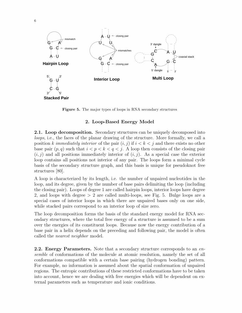
Figure 5. The major types of loops in RNA secondary structures

2. Loop-Based Energy Model

2.1. Loop decomposition. Secondary structures can be uniquely decomposed intoloops, i.e., the faces of the planar drawing of the structure. More formally, we call aposition k immediately interior of the pair (i, j) if i < k < j and there exists no otherbase pair (p, q) such that i < p < k < q < j. A loop then consists of the closing pair(i, j) and all positions immediately interior of (i, j). As a special case the exteriorloop contains all positions not interior of any pair. The loops form a minimal cyclebasis of the secondary structure graph, and this basis is unique for pseudoknot freestructures [80].

A loop is characterized by its length, i.e. the number of unpaired nucleotides in theloop, and its degree, given by the number of base pairs delimiting the loop (includingthe closing pair). Loops of degree 1 are called hairpin loops, interior loops have degree2, and loops with degree > 2 are called multi-loops, see Fig. 5. Bulge loops are aspecial cases of interior loops in which there are unpaired bases only on one side,while stacked pairs correspond to an interior loop of size zero.

The loop decomposition forms the basis of the standard energy model for RNA sec-ondary structures, where the total free energy of a structure is assumed to be a sumover the energies of its constituent loops. Because now the energy contribution of abase pair in a helix depends on the preceding and following pair, the model is oftencalled the nearest neighbor model.

2.2. Energy Parameters. Note that a secondary structure corresponds to an en-

semble of conformations of the molecule at atomic resolution, namely the set of allconformations compatible with a certain base pairing (hydrogen bonding) pattern.For example, no information is assumed about the spatial conformation of unpairedregions. The entropic contributions of these restricted conformations have to be takeninto account, hence we are dealing with free energies which will be dependent on ex-ternal parameters such as temperature and ionic conditions.

7

Table 1. Free energies for stacked pairs in kcal/mol.Note that both base pairs have to be read in 5’-3’ direction.

CG GC GU UG AU UACG −2.4 −3.3 −2.1 −1.4 −2.1 −2.1GC −3.3 −3.4 −2.5 −1.5 −2.2 −2.4GU −2.1 −2.5 1.3 −0.5 −1.4 −1.3UG −1.4 −1.5 −0.5 0.3 −0.6 −1.0AU −2.1 −2.2 −1.4 −0.6 −1.1 −0.9UA −2.1 −2.4 −1.3 −1.0 −0.9 −1.3

G

A

5’

5’

3’

3’U

C

−2.4kcal/mol

Qualitatively, the major energy contributions are base stacking, hydrogen bonds,and loop entropies. While hydrogen bond and stacking energies in vacuo can becomputed using quantum chemistry, the secondary structure model considers freeenergy differences between folded and unfolded states in an aqueous solution withrather high salt concentrations. As a consequence one has to rely on empirical energyparameters.

Energy parameters are typically derived by following the unfolding of RNA oligomersusing A collection of energy parameters is maintained by the group of David Turner[145, 90, 91]. These standard parameters are measured in a buffer of 1M NaCl at37C. As example we list the free energies for stacked pairs in table 1. Stacked pairsconfer most of the stabilizing energy to a secondary structure, a single additional basepair can stabilize a structure by up to −3.4 kcal/mol. For comparison, the thermalenergy1 at room temperature is about RT = 0.6kcal/mol, i.e., the stabilizing energycontribution of a single base pair is typically of the same order of magnitude as thethermal energy.

In general, loop energies depend on the loop type and its size. Except for smallloops (which are tabulated exhaustively [91]), sequence dependence is conferred onlythrough the base pairs closing the loop and the unpaired bases directly adjacent tothe pair. Thus, the loop energy takes the form

Eloop = Emismatch + Esize + Especial (1)

where Emismatch is the contribution from unpaired bases inside the closing pair andthe base pairs immediately interior to the closing pair. The last term is used e.g.to assign bonus energies to unusually stable tetra loops, such as hairpin loops withthe sequence motif GNRA. Polymer theory predicts that for large loops Esize shouldgrow logarithmically. For multi-loops, however, energies that are linear in loop sizeand loop degree have to be used in order to allow efficient dynamic programmingalgorithms for structure prediction. While the model allows only Watson-Crick (AU,UA, CG and GC) and wobble pairs (GU, UG), non-standard base pairs in helices aretreated as special types of interior loops in the most recent parameter sets.

The energy model above contains inaccuracies, on the one hand because it assumesthat loop energies are strictly additive, on the other hand because energy parameterscarry experimental errors (typically about 0.1 kcal/mol). Most seriously, the sequence

1RNA energy parameters are still published in kcal/mol to facilitate comparison with previousparameter sets. 1kcal/mol ≈ 4.2 kJ/mol in SI units.

8

dependence of loop energies has to be kept relatively simple, in order to deduce theparameters from a limited number of experiments.

2.3. Notes. Adjacent helices in multi-loops may stack co-axially to form a singleextended helix. tRNA structures are prominent examples of this. In the four armedmultiloop the acceptor stem co-axially stacks on the T stem, the anticodon stemstem stacks on the D-arm. This results in two extended helices which then form theL-shaped tertiary structure characteristic for tRNAs, see Fig. 1. Strictly speaking,co-axial stacking goes beyond the secondary structure model, since one has to knowwhich helices in the loop will stack in order to include the energetic effect; the listof base pairs is no longer sufficient information to compute the energy. Co-axialstacking is also cumbersome to include in structure prediction algorithms. It has,however, been shown to improve prediction quality [135]. Useful energy parametersfor structures with pseudoknots have so far only been collected for simple H-typepseudoknots [41].

3. The RNA Folding Problem

3.1. Counting structures and maximizing base pairs. In order to understandthe basic ideas behind the dynamic programming algorithms for RNA folding, it isinstructive to first consider the underlying combinatorial problem: Given an RNA

sequence x of length n, enumerate all secondary structures on x. Let xi denote thei-th position of x. We will simply write “(i, j) pairs” to mean that the nucleotides xi

and xj can form a Watson Crick or a wobble pair, i.e., xixj is one of GC, CG, AU,UA, GU, or UG. A subsequence (substring) will be denoted by x[i..j]. For notationalconvenience we interpret x[j + 1..j] as the empty sequence and associate a singleempty structure with it.

The basic idea is that a structure on n nucleotides can be formed in only two distinctways from shorter structures: Either the first nucleotide is unpaired, in which caseit is followed by an arbitrary structure on the shorter sequence x[i + 1..j], or thefirst nucleotide is paired with some partner base, say k. In the latter case the rulethat base pairs must not cross implies that we have independent secondary structureson the sub-intervals x[i + 1..k − 1] and x[k + 1..j]. Graphically, we can write thisdecomposition of the set of structures like this:

i jj i i+1 j i i+1 k−1 k k+1|=

It is now easy to compute the number Nij of secondary structures on the subsequencex[i..j] from positions i to j [140, 139]:

Nij = Ni+1,j +∑

k, (i,k) pairs

Ni+1,k−1Nk+1,j (2)

with Nii = 1. The independence of the structures on x[i + 1..k − 1] and x[k +1..j] implies that we can simply multiply their numbers. This simple combinatorial

9

structure of secondary structures was realized by M. Waterman in the late 1970s[140, 139].

Historically, the first attempts at secondary structure prediction tried to maximize thenumber of base pairs in the structure. The solution to this problem by the Nussinovalgorithm [101] is very similar to the combinatorial recursion above. Denote by Eij

the maximal number of base pairs in a secondary structure on x[i..j]. Using thedecomposition of the structure set, we see that Eij is the optimal choice among eachof the alternatives. In this context, independence of two substructures in the pairedcases implies that we have to optimize these substructures independently. If we like,we can associate each base pair with a weight (negative energy) βij which dependson xi and xj; we arrive immediately at the recursion

Eij = max

Ei+1,j , max

k, (i,k) pairsEi+1,k−1 + Ek+1,j + βik

(3)

Replacing the weights by binding energies (which are negative for stabilizing inter-actions) we simply have to replace max by min in the above recursions. In practice,this simplified energy model does not lead to reasonable predictions in most cases.We use it here for didactic purposes and relegate as more detailed description of thecomplete RNA folding problem to subsection 3.3.

The energy contributions of individual base pairs are in the same order of magni-tude as the thermal energy at room temperature. Thus RNA molecules exist in adistribution of structures rather than in a single ground-state structure. Thermody-namics dictates that, in equilibrium, the probability of a particular structure Ψ isproportional to its Boltzmann factor exp(−E(Ψ)/RT ). Here E(Ψ) is the energy ofthe sequence in conformation (secondary structure) Ψ, R is the molar gas constant(Boltzmann’s constant in molar units), and T the absolute ambient temperature inKelvin. This ensemble of structures is determined by its partition function

Z =∑

Ψ

exp(−E(Ψ)/RT ) , (4)

or, equivalently, by the free energy ∆G = −RT ln Z. The partition function Z canbe computed in analogy to equ. (3). Using Zij as the partition function over allstructures on sub-sequence x[i..j] we obtain [93]

Zij = Zi+1,j +∑

k, (i,k) pairs

Zi+1,k−1Zk+1,j exp(−βik/RT ) . (5)

Note that we can transform the recursion for Eij in equ.(3) into the equation for Zij

simply by exchanging maximum operations with sums, sums with multiplications,and energies by their corresponding Boltzmann factors.

The partition function allows to compute the equilibrium probability of a structureΨ as p(Ψ) = exp(−E(Ψ)/RT )/Z. The formalism is also used to efficiently computethe equilibrium probability of a base pair pij =

∑(i,j)∈Ψ p(Ψ). To this end one needs

to compute the partition function Zij of structures outside the subsequence x[i..j]using a recursion similar to the one above for Z. We can now compute the partition

10

Table 2. Comparison of backtracing recursions for different algorithms.

∅→ S.while S 6= ∅ do

π ← S;if π is complete then output π[i, j] = I ∈ Υπ.π′ = πJ (i + 1)if E(π′) = Eopt then π′ → S;next;for all k ∈ [i, j] do

π′ = πJ (i, k)if E(π′) ≤ Eopt

then π′ → S; next;

∅→ S.while S 6= ∅ do

π ← S;if π is complete then output πfor all [i, j] = I ∈ Υπ do

π′ = πJ (i + 1)if E(π′) ≤ Eopt + ∆Ethen π′ → S;for all k ∈ [i, j] do

π′ = πJ (i, k)if E(π′) ≤ Eopt + ∆Ethen π′ → S;

∅→ S.while S 6= ∅ do

π ← S;if π is complete then output πfor all [i, j] = I ∈ Υπ do

π′ = πJ (i + 1)π′ → S with probabilityZ(π′)/Z(π)for all k ∈ [i, j] do

π′ = πJ (i, k)π′ → S

with prob. Z(π′)/Z(π)

Algorithm B1. [101, 149]Backtracing a single structure

Algorithm B2. [144]Backtracing multiple struc-tures

Algorithm B3. [21]Stochastic backtracing

function over all structures containing the pair (i, j) and thus its probability

pij = ZijZi+1,j−1 exp(−βij/RT )/Z . (6)

Further variants of this scheme can be employed to compute e.g. the number of stateswith a given energy, to explicitly list all possible structures, or to determine structuresthat optimize other properties. In section 5.5 we will briefly mention how such variantscan be constructed in a systematic way within the framework of Algebraic Dynamic

Programming [37].

3.2. Backtracing. Recursion (3) computes only the optimal energy, not an optimalstructure which realizes this energy. This is typical for most dynamic programmingalgorithms: one first compute the value of the optimum, then uses backtracing (some-times called backtracking) to generate one (or more) structures in a step-wise fashionbased on the information collected in the forward recursions. This section closelyfollows an exposition of the topic in [27]. The basic object is a partial structure πconsisting of a collection Ωπ of base pairs and a collection Υπ of sequence intervalsin which the structure is not (yet) known. Positions that are known to be unpairedcan easily be inferred from this information. The completely unknown structure onthe sequence interval [1, n] is therefore ∅ = (∅, [1, n]) while a structure is complete

if it is of the form π = (Ω, ∅).

Suppose I = [i, j] ∈ Υ are positions for which the partial structure π = (Ω, Υ)is still unknown. If we know that i is unpaired then π′ = (Ω′, Υ′) with Ω′ = ΩΥ′ = Υ \ I ∪ [i + 1, j]. If (i, k), i < k ≤ j, is a base pair then Ω′ = Ω ∪ (i, k)and Υ′ = Υ \ I ∪ [i + 1, k− 1], [k + 1, j]. Here we use the convention that emptyintervals are ignored. Furthermore, base pairs can only be inserted within a singleinterval of the list Υ. We write π′ = πJ(i) and π′ = πJ(i, k) for these two cases.

11

The energy of a partial structure π is defined as

E(π) =∑

(k,l)∈Ω

βkl +∑

I∈Υ

Eopt(I) , (7)

where Eopt(I) = Eij is the optimal energy for the substructure on the interval I = [i, j]

The standard backtracing for the minimal energy folding starts with the unknownstructure. Instead of a recursive version we describe here a variant where incompletestructures are kept on a stack S. We write π ← S to mean that π is popped fromthe stack and π → S to mean that π is pushed onto the stack.

If we want all optimal energy structures instead of a single representative we simplytest all alternatives, i.e., we omit the next in the algorithm above. It is now almosttrivial to modify the backtracing to produce all structures within an energy bandEopt ≤ E ≤ Emax above the ground state.

Stochastic backtracing procedures for dynamic programming algorithm such as pair-wise sequence alignment are well known [97]. Replacing Zij by Nij in Algorithm B3we recover recursions for producing a uniform ensemble of structures similar to theprocedure for producing random structures without sequence constraint used in [126].

Note that the probabilities of π J (i + 1) and π J (i, k) for all k add to 1 so that ineach iteration we take exactly one step. Hence we simply fill one structure which weoutput as soon as it is complete.

3.3. Energy minimization in the loop-based energy model. Using the loopbased energy model is essential in order to achieve reasonable prediction accura-cies. As we shall see, the more complicated energy model results in somewhat morecomplicated recursions and requires additional tables. However, memory and CPUrequirements are still O(n3) and O(n2). The main difference to the simple model dis-cussed in the previous sections is that we now have to distinguish between differenttypes of loops. Thus we have to further decompose the set of substructures enclosedby the base pair (i, k) according to the loop types: hairpin loop, interior loop, andmulti(branched) loops, see Fig. 6. The hairpin and interior loop cases are simple sincethey reduce again to the same decomposition step.

The multiloop case is more complicated, however, since the multiloop energy dependsexplicitly on the number of substructures (“components”) that emanate from the loop.We therefore need to decompose the structures within the multiloop in such a waythat we can at least implicitly keep track of the number of components. To this endwe represent a substructure within a multiloop as a concatenation of two components:An arbitrary 5’ part that contains at least one component and a 3’ part that startswith a base pair and contains only a single component. These two types of multiloopsubstructures are now decomposed further into parts that we already know: unpairedintervals, structures enclosed by a base pair, and (shorter) multiloop substructures,see Fig. 6. It is not too hard to check that this decomposition really accounts for allpossible structures and that each secondary structure has a unique decomposition.

Given the recursive decomposition of the structures, we can now rather easily derivethe associated energy minimization algorithm. We will use the abbreviations H(i, j)

12

M1 M1

M1

i u u+1|

MC

= |

= | |

FC

i j i+1 j i

hairpin Cinterior

i j i i k l j

k k+1 j

=

C

F F

i j

M

=i ij j−1

| Ci j

M

ui+1 u+1i j−1 j

j i

M

j−1 j|C

i u u+1

j

j

j

Figure 6. Decomposition of RNA secondary structure. Dotted lines indicate unpairedsubstructures, while full length denote arbitrary structures; base pairs are indicated as arcs.Multiloop contributions with an arbitrary number of components are shown as irregular“mountains”. See text for further details.

for the energy of a hairpin loop closed by the pair (i, j), similarly I(i, j; k, l) shalldenote the energy of an interior loop determined by the two base pairs (i, j) and(k, l). We will also tabulate the following quantities:

Fij free energy of the optimal substructure on the subsequence x[i..j].Cij free energy of the optimal substructure on the subsequence x[i..j] subject to

the constraint that i and j form a base pair.Mij free energy of the optimal substructure on the subsequence x[i..j] subject to

the constraint that that x[i..j] is part of a multiloop and has at least onecomponent.

M1ij free energy of the optimal substructure on the subsequence x[i..j] subject to

the constraint that that x[i..j] is part of a multiloop and has exactly onecomponent, which has the closing pair i, h for some h satisfying i < h ≤ j.

The recursions for computing the minimum free energy of an RNA molecule in theloop based energy model were first formulated by Zuker & Stiegler [149]. They canbe summarized as follows:

Fij =min

Fi+1,j, min

i<k≤j

(Cik + Fk+1,j

)

Cij =min

H(i, j), min

i<k<l<j

(Ckl + I(i, j; k, l)

), min

i<u<j

(Mi+1,u + M1

u+1,j−1 + a)

Mij =min

mini<u<j

((u− i + 1)c + Cu+1,j + b

), min

i<u<j

(Mi,u + Cu+1,j + b

), Mi,j−1 + c

M1ij =min

M1

i,j−1 + c, Cij + b

,(8)

where we assume linear multiloop energies of the form EML = a + b · degree + c · size.In contrast to most implementations the version shown here decomposes structures

13

in such a way that each substructure occurs exactly once. While this is not strictlynecessary for energy minimization, it allows us to use essentially the same recursionsfor all variants of the problem, including the computation of the partition functionor the backtracing of all or a sample of suboptimal structures.

3.4. RNA Hybridization. Intermolecular base pairing between two RNA moleculescan be treated in the same way as intramolecular interactions. The most straightfor-ward approach is to concatenate the two molecules. One can then apply the foldingalgorithms for single molecules. There is only a single necessary modification to thefolding algorithms: the energy contribution of the loop that contains the cut point isdifferent. Implementations of this approach are RNAcofold [58] and pairfold [5].

¿From a physics point of view, however, additional effects need to be taken intoaccount: the interaction of two distinct molecules is concentration dependent. Fur-thermore, there is an additional (entropic) contribution for the initiation of an in-termolecular interaction. The extension of the folding algorithms of course computeboth inter- and intra-molecular contributions. It is therefore necessary to correct forthe initialization energy Ei:

ZAA = (ZAA − Z2

A) exp(−Ei/RT ) ,

ZBB = (ZBB − Z2

B) exp(−Ei/RT ) , and

ZAB = (ZAB − ZAZB) exp(−Ei/RT ) .

(9)

where Z is the partition function as calculated from the folding algorithm for the con-catenated sequences, ZA and ZB are the partition functions of the isolated moleculesA and B. Standard statistical thermodynamics can then be used to compute theconcentration dependencies of the complex formation, see e.g. [20] for a discussion inthe context of RNA hybridization.

Various simplified approaches have been discussed in recent years. In particular,the most common approximation is to neglect the secondary structures of the twointeracting molecules. This amounts to a model in which the concatenated structurecan only have base pairs and interior loops and the cut point is located in the singlehairpin loop. It does, however, result in a much faster algorithm with time complexityO(n ·m) instead of O((n + m)3) for two sequences of length n and m. Algorithmsfor this case have been described in [20] and [105]; the Vienna RNA Package alsoprovides an implementation. The RNAhybrid program was in particular used to detectmicroRNA/target interactions.

3.5. Pseudoknotted Structures. Many functionally important RNA structurescontain pseudoknots, including rRNAs [12], RNase P RNAs [10, 49], and tmRNA[151]. Recently, algorithms have been described that are able to deal with certainclasses of pseudoknotted structures. As we shall see below, these are however plaguedby considerable computational costs. In addition, a common problem of all theseapproaches is the still very limited information about the energetics of pseudoknots[41, 66].

14

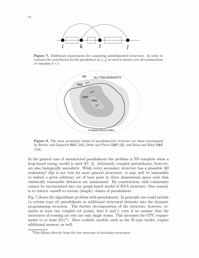
i k l j

Figure 7. Additional requirements for computing pseudoknotted structures. In order toevaluate the contribution for the pseudoknot on [i, j] we need to iterate over all combinationsof cutpoints k < l.

PLANAR STRUCTURES

N 6

R&G

N 4

N 5

D&P

ALL PSEUDOKNOTS

R&E

NP

Figure 8. The most prominent classes of pseudoknotted structure are those investigatedby Reeder and Giegerich R&G [104], Dirks and Pierce D&P [22], and Rivas and Eddy R&E

[110].

In the general case of unrestricted pseudoknots the problem is NP-complete when aloop-based energy model is used [87, 3]. Arbitrarily complex pseudoknots, however,are also biologically unrealistic. While every secondary structure has a plausible 3Drealization2 this is not true for more general structures: it may well be impossibleto embed a given arbitrary set of base pairs in three dimensional space such thatchemically reasonable distances are maintained. By construction, such constraintscannot be incorporated into our graph-based model of RNA structure. One remedyis to restrict oneself to certain (simple) classes of pseudoknots.

Fig. 7 shows the algorithmic problem with pseudoknots. In principle one could include(a certain type of) pseudoknots as additional structural elements into the dynamicprogramming recursion. The further decomposition of the structure, however, re-quires at least two coupled cut points, here k and l, even if we assume that thestructures of crossing arc sets are only single stems. This increases the CPU require-ments to at least O(n4). More realistic models, such as the H-type model, requireadditional memory as well.

2This follows directly from the tree structure of secondary-structures.

15

Algorithms for a number of different classes of pseudoknots have been published inrecent years, see e.g. [110, 3, 87, 104, 22]. Fig. 8 summarizes the relationships betweenthe algorithmic complexities of predicting secondary structures from some of thesestructure classes [16].

3.6. Notes. The basic counting recursion can be readily modified to enumerate otherquantities of interest such as the structures with particular properties and distribu-tions of structural elements, see e.g. [55]. The combinatorics of RNA secondarystructures and related mathematical objects such as ordered trees, Motzkin paths,and non-crossing partitions is still an active area of research, see e.g. [13, 19, 81] andthe references therein.

The recursions for the loop-based energy model as displayed above, in fact, give riseto O(n4) CPU requirements due to the interior loop contribution. However, very longinterior loops are extremely unlikely (and unstable), so that the length of interior canbe bounded by a constant, e.g. M = 30. The interior loop contribution thus remainsquadratic. Under certain plausible assumptions on the interior loop energies, a cubictime algorithm can be designed [86] that takes interior loops of all sizes into account.

A restriction of the folding algorithm to local structure is described in [52]. Herethe maximum span |j − i + 1| of a base pair (i, j) is bounded by a constant L. Theresulting “scanning” algorithms are linear in time and space and hence can be usedto screen entire genomes for locally stable structures.

Circular RNA molecules are rare, but their secondary structures are of consider-able interest because structural features are important e.g. in viroids [123, 108]. Astraightforward way of dealing with circular RNA molecules is to compute Cij andMij also for the subsequences of the form x[j..n]x[1..i] [150]. The disadvantage ofthis approach is, however, that it doubles the memory requirements. An alternativeis described in [60].

A secondary structure Ω is saturated if none of its stems can be elongated, i.e.,if any single base pair that is inserted into Ω does not stabilize the structure bystacking to any other base pairs. The recursions Fig. 6 can be modified to produceonly saturated structure [26]. Similarly, we may call Ω locally base pair optimal if Ωcannot be expanded by any additional base pair. In [15] an dynamic programmingalgorithm is described that computes such locally optimal structures in quartic timewith cubic memory requirements.

Prediction of pseudoknotted structures based on maximum matching can be doneusing algorithms for Maximum Weighted Matching [125]. While this approach re-quires only O(n3) time, it cannot take the loop based energy model into account.“Iterated loop matching”, i.e., the repeated (greedy) application of the Nussinov al-gorithm, is another approximate way of computing pseudoknotted structures [113].Finally, heuristics such as genetic algorithms can be used to compute pseudoknottedstructures [78].

16

4. Conserved Structures, Consensus Structures, and RNA Gene Finding

4.1. The Phylogenetic Method. Most functional RNA molecules have charac-teristic secondary structures that are highly conserved in evolution. Well knownexamples include rRNAs, tRNAs, RNAse P and MRP RNAs, the RNA componentof signal recognition particles, tmRNA, group I and group II introns, and small nu-cleolar RNAs. It is therefore of considerable practical interest to efficiently computethe consensus structure of a collection of such RNA molecules.

Given a sufficiently large database of aligned RNA sequences, one can directly infer aconsensus secondary structure from the data. The basic idea is that substitutions inthe sequence will respect the common structural constraints: Therefore, substitutionsin helical regions have to be correlated, since in general only 6 (GC, CG, AU, UA,UG, and GU) out of the 16 combinations of two bases can be incorporated in thehelix. Two columns in the alignment thus will co-vary if they form a base pair.

For concreteness, assume that we are given a multiple sequence alignment A of Nsequences. By Ai we denote the i-th column of the alignment, while aα

i is the entryin the α-th row of the i-th column. The length of A, i.e., the number of columns,is n. Furthermore, let fi(X) be the frequency of base X at aligned position i and letfij(XY) be the frequency of finding simultaneously X at position i and Y at j.

The most common way of quantifying sequence covariation for the purpose of RNAsecondary determination is the mutual information score [14, 45, 44]

MIij =∑

X,Y

fij(XY) logfij(XY)

fi(X)fj(Y)(10)

Usually, the mutual information score makes no use of RNA base-pairing rules. Forlarge datasets this is desirable, since it allows to identify non-canonical base pairs andtertiary interaction. For the small datasets considered in the following subsections,however, neglecting base pairing rules does more harm (by increasing noise) thangood. In particular, mutual information does not account at all for consistent non-compensatory mutations, i.e., if we have, say, only GC and GU pairs at positions iand j then Mij = 0. Thus sites with two different types of base pairs are treated justlike a pair of conserved positions.

A straightforward measure of covariation takes the form

Cij =∑

XY,X′Y′

fij(XY)DXY,X′Y′fij(X′Y′). (11)

where a suitable choice for the 16×16 matrix D has entries DXY,X′Y′ = dH(XY, X′Y′) ifboth XY ∈ B and X′Y′ ∈ B and DXY,X′Y′ = 0 otherwise. Here B = GC, CG, AU, UA, GU, UG

and dH(XY, X′Y′) is the Hamming distance of XY and X′Y′. The idea here is that con-sistent mutations such as GC → GU should count less (here half) of a compensatorymutation such as GC→ AU. Note that equ.(11) is a scalar product, Cij = 〈fijDfij〉,and hence can be evaluated efficiently. If desired, D could be replaced by a differentkernel that e.g. could incorporate measured substitution rates [35].

17

The purely phylogenetic approach suffers from two limitations: (1) It requires a verylarge set of sequences in order to obtain a reliable estimate of covariance or mutualinformation for each pair of sequences. With the exception of rRNAs and tRNAs,such large datasets are usually not (yet) available. (2) It is sensitive to alignmenterrors, and hence not applicable to very diverse sets of sequences. A possibly rem-edy is provided by approaches towards solving the folding and alignment problemssimultaneously or iteratively. These are discussed in the following section.

4.2. Conserved Structures. The amount of data that is required for inferringstructures can be reduced dramatically by taking thermodynamics of folding intoaccount. Indeed, [47] suggested to resolve ambiguities in the phylogenetic analysisbased on thermodynamic considerations.

The converse approach, however, namely to use the information which base pairsare thermodynamically plausible, appears to be more efficient. Most of the align-ment based methods therefore start from thermodynamics-based folding and use theanalysis of sequence covariations or mutual information for post-processing, see e.g.,[77, 84, 85, 54, 59, 71]. We describe here the alidot algorithm [54, 59].

For each of the aligned sequences secondary structures are computed separately. Theresulting lists of base pairs from either minimum free energy calculations or from apartition function calculation are then superimposed by using the multiple sequencealignment to determine which pairs in different sequences are equivalent. For eachpair we now have both thermodynamic and sequence covariation information, whichis used to hierarchically rank order base pairs depending on their support across theentire data set. A greedy procedure then extracts contiguous stems from the rankordered list and combines them to a partial secondary structure which contains onlythose sequence/structure elements that are significantly conserved throughout thealigned input sequences.

Sequence andPairing Probability

Extract valid secondary structure

UGUGGUCGAUAU 0.90

0.650.450.100.770.34

sec. structure

Extract several Layers of valid

* inconsistent mutations* mean probability

Credibility Ranking

* compensatory mutations

depending on

[[[.......]]]..........

....(((((......)))))...

...................

[[[.(((((.]]]..)))))...

. . .. . .. . .. . .

. . .

. . .. . .. . .

.

..

.. .. ..

... . .

. . .. . .

. . .

. . ... .. ... . .. . ..

..

...

...

. .

.... .

....

.

..

.. . .

......

.. . . ..

...

......

.

. . ... .. ... . ... .. ..

Multiple Sequence Alignments

Dot Plots

RNA Sequences

Combined Pair Table

Conserved sub−structures

McCaskill’s Algorithm

ClustalW

Figure 9. Flow chart of the alidot algorithm.

18

An alternative to the ranking/greedy approach of alidot is to compute a score orweight wij for each possible base pair. The program ConStruct [85] uses a simplescoring function that exclusively combines the base pairing probabilities of the indi-vidual sequences. Covariance or mutual information score as well as contributionsthat consider the potential to extend the pair to a longer helix [141] could easily beincluded. A secondary structure can then be computed using the Nussinov algorithmwith weights wij for the base pairs. The downside of this approach is that it returnsa global secondary structure rather than a collection of well-supported local features.

Comparative approaches are based on the fact that RNA secondary structure is quitefragile against randomly placed point mutations. Our earlier computational stud-ies suggest, that even with 85% sequence identity we should expect no significantstructural similarity [33, 116]. While this result may seem surprising, there has beenconvincing experimental evidence, see e.g. [115]. Methods such as alidot thus candiscriminate very well between conserved and non-conserved RNAs. Both alidot andConStruct require interactive work and are therefore best suited for small genomesas found in RNA viruses [142, 131, 56].

4.3. Consensus Structures. Sometimes it is known a priori that the aligned se-quences should fold into a common secondary structure. This is the case e.g. forrRNAs, tRNAs, and many other small non-coding RNA molecules. In this case itmakes sense to ask, what is the most stable structure that can be formed simulta-neously by all (or almost all) input sequences. This problem is solved in a ratherstraightforward way by RNAalifold [53]. It treats the entire alignment like a singlesequence and solves the secondary structure problem for this “generalized sequence”.To this end, of course, an extension of the standard energy model to alignments isrequired. RNAalifold simply averages the energy contribution over all sequences. Inthe simple case of base pair dependent energies this means

βA

ij =1

N

∑

α

βxαi ,xα

j(12)

For the realistic energy model, energies for the different loop types are averagedindividually.

Both the mutual information score and the covariance score assign a bonus to compen-satory mutation. Neither score deals with inconsistent sequences, i.e., with sequencesthat cannot form a base pair between positions i, j. The simplest ansatz for thispurpose is to simply count the number of sequences qij that cannot form a canonicalbase pair between columns i and j. Here, combinations of a nucleotide and a gap arecounted as inconsistent while gap-gap combinations (i.e. deletions of an entire basepair) are ignored.

In a multiple alignment of a larger number of sequences we have to expect occasionalsequencing errors and of course there will be alignment errors. Thus we cannotsimply mark a pair of positions as non-pairing if a single sequence is inconsistent.Furthermore, there is the possibility of a non-standard base pair [44]. Thus we definea threshold value for the combined score Bij = Cij − φ1qij and declare a pair ofpositions i, j as non-pairing if Bij is too small.

19

Figure 10 shows the consensus structure of the mir-105 microRNA family as an ex-ample. Such consensus structures are needed for the derivation of pattern descriptionsthat can be used to search for structurally similar RNAs in genomic DNA, as brieflydescribed in the following section.

4.4. RNA Gene Finding. It is, of course, possible to identify genomic sequencesthat are homologous to known RNA genes, using either BLASTN or, as in the case oftRNAs, more specialized methods. For most functional noncoding RNA (ncRNA)molecules the secondary structure is much more conserved than their sequence. Thiscan be used to identify putative noncoding RNA sequences using programs such asRNAmot [34], tRNAscan [83], or HyPa [40]. Nevertheless, all these approaches arerestricted to searching for new members of the few well-established families such astRNAs, snoRNAs, microRNAs, and certain spliceosomal RNAs.

A different approach is taken in the program QRNA [111]. This method for compara-tive analysis of two aligned homologous sequences can detect novel structural RNAgenes by deciding whether the substitution pattern fits better with (a) synonymoussubstitutions, which are expected in protein-coding regions, (b) the compensatory

AUCUUCUGAGUGUGCAUCGUGGUCAAAUGCUCAGACUCCUGUGGUGGCUGCUCAUGCACCACGGAUGUUUGAGCAUGUGCUAUGGUGUCUACUUUUGCAAC_

0 10 20 30 40 50 60 70 80 90 100

AUC

UUCU

GA G

UG

UGCAUCGUGGUC

AAA

UGCUCAGAC

UC

CUGUGGUGGC

UG

C U CAU

GCACCACGG

AU

GUUUGAGCAU

GU

GCUAUGGUGU

CUAC U U

UUGC

AA

C_

CG

GCUA

UG

UG

CGGC

UA

UA

GC

CGAU

Figure 10. Consensus secondary structure of the 11 sequences from mammalian microRNAmir-105. Sequence are taken from the microRNA Registry (version 6.0) and from blast

searches in vertebrate genomes.L.h.s: Mountain plot: A base pair (i, j) is represented by a slab ranging from i to j. The 5’and 3’ sides of stems thus appear as up-hill and down-hill slopes, respectively, while plateausindicate unpaired regions. Colors indicate sequence variation by encoding the number ofdifferent types of base pairs (GC, CG, AU, UA,GU, UG) that occur in the two paired columnsof the alignment. Pairs with conserved sequence are shown in red; ocher, green, cyan, blue,violet indicate two to 6 types of base pairs. Pairs with one or two inconsistent mutations areshown in (two degrees of) pale colors.R.h.s.: In the conventional secondary structure graph paired positions are color coded as inthe mountain plot. Consistent mutations are indicated by circles around the varying position,compensatory mutations thus are marked by circles around both pairing partners.

20

mutations consistent with some base paired secondary structure, or (c) uncorrelatedmutations.

The alidot approach has never been used for large scale gene finding since it hasturned out to be non-trivial to assign statistical significance values to its results.Most recently, however, a conceptually related technique has been developed that isefficient and sensitive enough to allow genome-wide screens for RNAs.

The program RNAz [136] combines a comparative approach (scoring conservation ofsecondary structure) with the observation [76, 138, 8] that ncRNAs are thermody-namically more stable than expected by chance. This excess stability is convenientlymeasured in terms of the z-score

z =E − E

σ(13)

where E and σ are mean and standard deviation of the distribution of shuffled se-quences. Instead of dealing with individual sequences, RNAz uses multiple sequencealignments of potential RNAs from different species as input. The computation of thez by direct sampling is extremely time-consuming. In RNAz it is therefore replacedby a support vector machine that has been trained to solve the regression problemsof estimating E and σ from properties of the input sequences.

Structural conservation is also quantified in thermodynamical terms: The structureconservation index S is defined as the ratio of the average energy of the consensusstructure (as computed by RNAalifold) and the average of the unconstrained foldingenergies of the individual sequences. An alignment of identical sequences thus hasS = 1. On the other hand, completely unrelated sequences will not be able toform a consensus structure since there are always some sequences that contradictany particular pairing, thus S = 0. Sequences that form a well-conserved consensussequence in the presence of sequence covariations, finally, will have the same energycontributions in the consensus and in the individual folds. In addition, however, theconsensus energy contains the bonus contributions for sequence covariations, so thatwe obtain S > 1.

RNAz uses a support vector machine (SVM) [17] to determine from the z-score andthe structure conservation index whether a given multiple sequence alignment is astructurally conserved RNA. Surveys of animal genomes [137, 96] reveal a very largenumber of previously unknown candidates for both independent ncRNAs and struc-tured cis-acting elements in mRNAs.

4.5. Notes. Including covariation information is also a good way to improve theaccuracy of structure predictions including pseudoknots. One approach is to forgoa loop-based energy model and use base pair scores instead, in which case the re-sulting Maximum Weighted Matching problem can be solved efficiently [125]. Goodaccuracies can be achieved by using a combination of covariance and thermodynamiccriteria for scoring potential base pairs [141]. The ILM program of Ruan et al. [113],uses the Nussinov algorithm iteratively in order to build pseudoknotted structures.

21

0.0

0.2

0.4

0.6

0.8

1.0

1.2

0.0

0.2

0.4

0.6

0.8

1.0

1.2

0.0

0.2

0.4

0.6

0.8

1.0

1.2

-8 -6 -4 -2 0 20

0.2

0.4

0.6

0.8

1

1.2

-8 -6 -4 -2 0 2 -8 -6 -4 -2 0 2

5S rRNA tRNA SRP RNA

RNAseP RNA U2 snRNA U5 snRNA

U3 snoRNA U70 snoRNAHammerheadribozyme III

Group IIcatalytic intron tmRNA microRNA mir-10

z-score

Str

uctu

re c

onse

rvat

ion

inde

x

Figure 11. Scatter plot of structure conservation index S (x-axis) and energy z-score (y-axis) for different families of structured non-coding RNAs. In each panel, the properties ofthe true sequences (dark) are compared with controls obtained by shuffling the sequence.Data are taken from [136].

22

u a

C

g c

a a a

C

L’c g

Cg c

g cL’a a u

L Ca

AGCC

GUCA

GG

AA U

CC G

CA A

AGC

GAG

GGC

F

C

C

c gL C L

Fa

C

M N

g c

c g

g g

c g

Figure 12. Parse tree and secondary structure drawing for a small example structure, usingthe grammar from equ.(15). Productions of the form L→ ∅ are left out for simplicity.

5. Grammars for RNA Structures

5.1. Context Free Grammars and RNA Secondary Structures. The recur-sions for RNA folding in Fig. 6 suggest a close connection with certain grammars.More precisely, we may interpret Fig. 6 as the production rules of an “RNA language”.The tree representations in Fig. 4, on the other hand are suggestive of a connectionbetween RNA structures and parse trees of a grammar that generates RNA sequence.As we shall see in this section, these connections can be made precise and open thedoor to the application of learning techniques in RNA bioinformatics.

Recall that a formal language L is a set of strings over a given alphabetA. A grammar

G for the language L consists of

• a set T of terminals which are the letters of the alphabetA possibly augmentedby the null-character ε.• a set N of non-terminals which represent the syntactic categories of L• a set P of production or derivation rules which are used to derive the strings

in L. Each production consists of a non-terminal “head” that is producedand a string of zero or more non-terminal and terminals (the “body” of theproduction)• a single non-terminal S ∈ N that is designated as the start symbol.

The “dot-parenthesis” grammar for RNA, in the simplest case, can be written asG0 = (T, N, P, s) with T = (, ), ., ∅, N = S, s = S, and

P =S → S., S → (S)S, S → ∅

, (14)

where ∅ denotes the empty string. The grammar above is context-free since allproductions are of the form V → w, where V is a non-terminal and w is a stringconsisting of terminals and/or non-terminals. The grammar generates strings of dotsand balanced parenthesis, the parse trees of this grammar correspond to the sec-ondary structures. More elaborate grammars can be designed that explicitly encodedifferent types of loops or other substructures. In particular, the decompositions ofthe structure sets in section 3.3 can be recast in terms of a grammar:

23

F → uF |CF |∅

C → pL′p | pLCLp | pMNp

M → LC | MC | Mu

N → Nu | C

L′ → uuuL

L→ uL | ∅

(15)

This grammar generates RNA sequences, while again the parse trees correspond tosecondary structures. The terminal u denotes an unpaired base, while p and p isa shorthand for one of the six pairing combinations of bases. The start symbol Frepresents any structure, L stands for an unpaired sequence within a loop, M and NThe production for L′ enforces the minimum length of a hairpin loop.

Chomsky normal forms have only productions of the form V → XY and V → awith V, X, Y ∈ N and a ∈ T . One can show that every context-free grammar canbe converted to normal form, i.e., there is a CFG in normal form that produces thesame language L.

Given a context-free grammar G = (T, N, P, s) we obtain a stochastic context-free

grammar (SCFG) by assigning probabilities P(α) to all productions α ∈ P such that∑α∈P P(α) = 1 is satisfied.

The probabilities associated with the individual productions take on the role of theenergy parameters in the previous sections. While the energy parameters must bemeasured directly, the values of P(α) can be inferred from training sets of knownsequence/structure pairs in a generic machine learning setting. Thus they can, at leastin principle, readily combine different sources of information that can be expressedprobabilistically, such as an evolutionary model (derived from a comparative analysisof RNA sequences) and a biophysically motivated model of structure plausibility. Inthe following three subsection we briefly outline the basic techniques: finding themost likely parse-tree, computing the probability of a given word, and the estimationof production probabilities from a given dataset. None of these algorithms is RNAspecific; they rather apply to any SCFG in Chomsky normal form.

5.2. CYK Algorithm. The analog of the minimum free energy folding problem inthe SCFG setting can be phrased in the following way: Given a string x ∈ L, findthe most likely parse tree for x in a grammar G.

Under the assumption that G is in Chomsky normal form, there is an efficient (polynomial-time) solution to this question the Cocke-Younger-Kasami (CYK) algorithm [146]:

Let w(i, j, V ) denote the likelihood of the most likely parse tree on the substring x[i..j]rooted at the nonterminal V . Clearly, we have w(i, i, V ) = log P(V → xi) for all i andV . For all larger substrings, j > i, we try all productions of the form V → XY andselect the one that maximizes the likelihood. This immediately leads to the recursion

w(i, j, V ) = maxX

maxY

maxi≤k<j

(log P(V → XY ) + w(i, k, X) + w(k + 1, j, Y )

)(16)

24

with the initialization w(i, i, V ) = log P(V → xi). The same type of backtracingapproach as in the Nussinov algorithm can be used to explicitly recover the parsetree, which corresponds to the secondary structure of the RNA molecule.

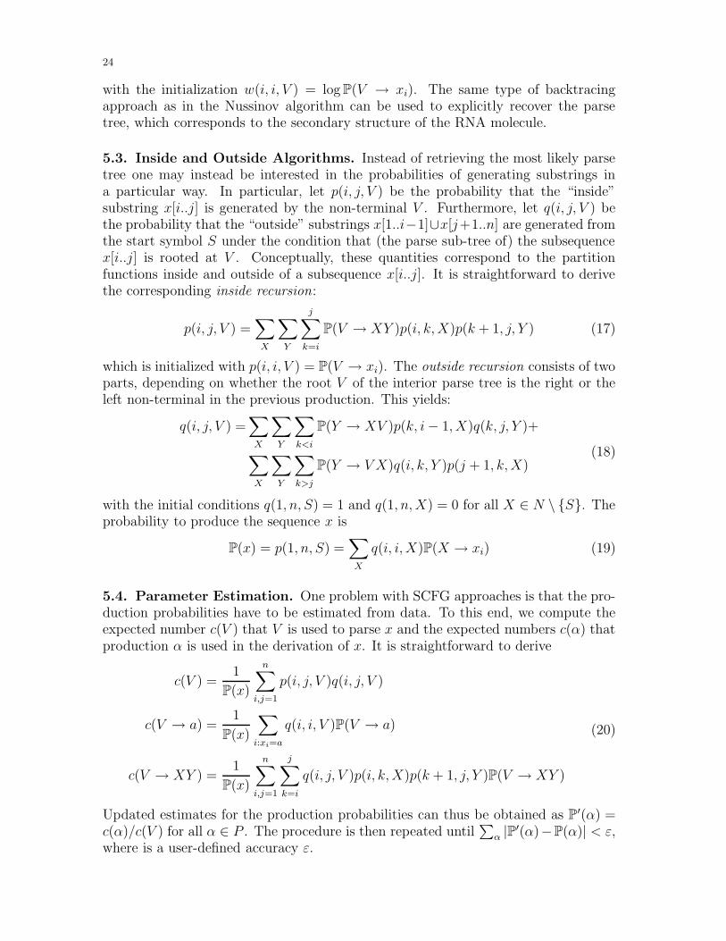
5.3. Inside and Outside Algorithms. Instead of retrieving the most likely parsetree one may instead be interested in the probabilities of generating substrings ina particular way. In particular, let p(i, j, V ) be the probability that the “inside”substring x[i..j] is generated by the non-terminal V . Furthermore, let q(i, j, V ) bethe probability that the “outside” substrings x[1..i−1]∪x[j+1..n] are generated fromthe start symbol S under the condition that (the parse sub-tree of) the subsequencex[i..j] is rooted at V . Conceptually, these quantities correspond to the partitionfunctions inside and outside of a subsequence x[i..j]. It is straightforward to derivethe corresponding inside recursion:

p(i, j, V ) =∑

X

∑

Y

j∑

k=i

P(V → XY )p(i, k, X)p(k + 1, j, Y ) (17)

which is initialized with p(i, i, V ) = P(V → xi). The outside recursion consists of twoparts, depending on whether the root V of the interior parse tree is the right or theleft non-terminal in the previous production. This yields:

q(i, j, V ) =∑

X

∑

Y

∑

k<i

P(Y → XV )p(k, i− 1, X)q(k, j, Y )+

∑

X

∑

Y

∑

k>j

P(Y → V X)q(i, k, Y )p(j + 1, k, X)(18)

with the initial conditions q(1, n, S) = 1 and q(1, n, X) = 0 for all X ∈ N \ S. Theprobability to produce the sequence x is

P(x) = p(1, n, S) =∑

X

q(i, i, X)P(X → xi) (19)

5.4. Parameter Estimation. One problem with SCFG approaches is that the pro-duction probabilities have to be estimated from data. To this end, we compute theexpected number c(V ) that V is used to parse x and the expected numbers c(α) thatproduction α is used in the derivation of x. It is straightforward to derive

c(V ) =1

P(x)

n∑

i,j=1

p(i, j, V )q(i, j, V )

c(V → a) =1

P(x)

∑

i:xi=a

q(i, i, V )P(V → a)

c(V → XY ) =1

P(x)

n∑

i,j=1

j∑

k=i

q(i, j, V )p(i, k, X)p(k + 1, j, Y )P(V → XY )

(20)

Updated estimates for the production probabilities can thus be obtained as P′(α) =

c(α)/c(V ) for all α ∈ P . The procedure is then repeated until∑

α |P′(α)−P(α)| < ε,

where is a user-defined accuracy ε.

25

5.5. Algebraic Dynamic Programming. Algebraic Dynamic Programming (ADP)[37] was introduced to facilitate and systematize the development of dynamic pro-gramming algorithms. Conceptually, a DP algorithm consists of three components: asearch space of candidate solutions (in our case RNA secondary structures), a scoringscheme (free energies, partition functions, etc.), and an objective function (minimize[energy], sum up [Boltzmann factors]). The idea behind ADP is to separate thesethree aspects. For a comprehensive discussion of ADP in the context of bioinfor-matics we refer to [37]. We can give here only a very brief, qualitative sketch of thetopic.

The search space is defined by a yield grammar, i.e., a tree grammar that generatesa string language by mapping its terminal symbols at the leaves of the tree intosequences of symbols. A tree grammar is similar to a context-free grammar, withterminal and non-terminal symbols, and productions where the right hand sides aretrees (formulas) from some underlying term algebra. Intuitively, first the search spaceis “constructed” by enumerating all candidate solutions. This is a parsing problemfor which standard solutions, so-called tabulating yield parsers, exist. Scoring andchoice are described in terms of an evaluation algebra which is independent of thedetails of the search space.

The main advantage is that complex variants of folding problems can be implementedvery easily: It suffices to modify the grammar to restrict the dynamic programmingrecursions to all canonical secondary structures, i.e., those that have no isolated basepairs. Conversely, the evaluation algebra can changed easily. Once the energy model isimplemented, one can change the choice function from minimizing energies to addingup Boltzmann factors or listing all structures within an energy range.

The restrictions of the search space can be quite dramatic: One can, for examplerestrict oneself to saturated secondary structures, which consist solely of maximallyextended stacking regions, i.e. no adjacent single stranded nucleotides exist that couldform a base pair and stack on top of a helix [26]. A particularly interesting applicationof the ADP framework is RNAshapes [36] which can be used to systematically generate(sub)optimal RNA structures belonging to distinct course-grained structural classes.For example, one can search for the most stable clover-leaf shaped secondary structurethat can be formed by the input sequence.

5.6. Notes. Due to space restrictions we only gave a brief sketch of the SCFG ap-proach to RNA secondary structures. A variety of implementations of SCFG-basedalgorithms are available for different purposes: pfold [75, 74] as an SCFG-approachto “folding an alignment” similar in spirit to the thermodynamics-based RNAalifold.

A general approach to computing suboptimal parse trees, similar in spirit to the back-tracing of RNA secondary structures with suboptimal energies, is described in [70].A systematic comparison of several alternative grammar models for RNA secondarystructures showed that the actual performance of SCFGs can depend considerably onthe details of the grammar being used [23].

A practical problem for the application of SCFGs is that one needs a grammar thatis both unambiguous and in Chomsky normal form. The decomposition of Fig. 6,

26

for example, does not satisfy this requirement, because the last case in the secondline, for example, requires non-terminals for the closing base pair as well as for thetwo enclosed multiloop components. Without discussing the details here, this createsproblems in particular with the multiloop decomposition.

Sean Eddy’s Infernal [25] creates a covariance model from local alignments andcan be used to search a sequence database for sequences that are likely to be pro-duced from this SCFG. Rsearch [73] aligns an RNA query to target sequences, usingSCFG algorithms to score both secondary structure and primary sequence alignmentsimultaneously.

So-called pair SCFGs can be used to solve the combined folding and alignment prob-lem in analogy to Sankoff’s algorithm described in the next section, see e.g. [64]. TheQRNA program [112] uses a pair SCFG to compute the probability that the substitutionpattern in a pairwise alignment is derived from RNA secondary structure conserva-tion. It has been used successfully to predict ncRNA candidates in E. coli and S.

cerevisiae [109, 94]. Most recently, Pedersen et al. [103, 102] devised an SCFG-basedalgorithm for detecting conserved secondary structure motifs specifically within cod-ing sequences. An SCFG-like approach to pseudoknotted structures can be found in[11].

6. Comparison of Secondary Structures

Many classes of functional RNA molecules, including tRNAs, rRNAs, and many other“classical” ncRNAs, are characterized by highly conserved secondary structures butlittle detectable sequence similarity. Reliable multiple alignments can therefore beconstructed only when the shared structural features are taken into account. Sincemultiple alignments are used as input for many subsequent methods of data analysis,structure based alignments are an indispensable necessity in RNA bioinformatics.This problem is far from being solved in a satisfactory way, both because the availableapproaches are computationally expensive, and because little is known about theevolution of RNA at the structural level, and hence on the appropriate edit costparameters.

6.1. String-Based Alignments. The problem of comparing two structures Ψ1 andΨ2 of the same RNA molecule is trivial: Since a secondary structures is simply a setof base pairs one may use for example the size of symmetric difference between thetwo sets |Ψ14Ψ2| as a distance measure that is obviously a metric. In other words,we simply count the number of base pairs that occur in one of the structures but notin both,

The question immediately becomes non-trivial, however, if we do not assume that thetwo structures have the same underlying sequence length, i.e., if we do not know a

priori which sequence positions in the two molecules correspond to each other.

As we have seen, RNA secondary structures can be faithfully represented as stringsover the alphabet (, ), .. Clearly, we can use this string representation to computea metric on secondary structures by means of standard sequence alignment methods,e.g. using the Needleman-Wunsch algorithm [99].

27

This approach can be generalized to a comparison of base pair probability matrices[7]. From the pairing probabilities of base i we construct a vector containing the prob-abilities of being paired upstream p<(i) =

∑j>i Pij, downstream p>(i) =

∑j<i Pji,

or unpaired p(i) = 1− p<(i)− p>(i). The resulting profiles can be aligned by meansof a standard string/profile alignment algorithm in O(n2) time using

ρ =√

p>Ap>

B +√

p<Ap<

B +√

pApB (21)

as the match score (or 1 − ρ as an edit cost). While this approach of “string-like

alignments” is fast, it often produces misaligned pairs:

Sequence alignment Structure alignmentCAGUCUCAGGUGGUUGGGCU- CAGUCUCAGGUGGUUG-GGCU.((((.(((....)))))))- .((((.(((....)))-))))UAG-CUGAGGUG-UCGUGCUA -UAGC-UGAGGUGUCGUGCUA(((-((((....-))).)))) -((((-(((....))).))))

Figure 13. Sequence vs. structure alignment. Compared to the structural alignment(right), the sequence alignment (from ClustalW) mis-aligns 5 of the 7 base pairs.

6.2. Tree Editing. The string-based alignments above essentially use only the in-formation whether a nucleotide is paired or unpaired, but neglect the connectivityinformation who pairs with whom. This limitation can be overcome by methodsbased on the tree representation of secondary structures. Of particular interest aretree editing and the related tree alignment, since they are still fast enough to beapplicable to genome wide surveys. We present these approaches in detail here sincethere does not appear be a good textbook exposition of this topic.

The three most natural operations (“moves”) that can be used to convert orderedtrees (and, more generally, ordered forests) into each other are depicted in Fig. 14:

(1) Substitution (x→ y) consists of replacing a single vertex label x by anothervertex label y.

(2) Insertion (∅ → z) consists of adding a vertex z as a child of x, therebymaking z the parent of a consecutive subsequence of children of x. A node zcan also be inserted at the “top level”, thereby becoming the root of a tree.

(3) Deletion (z → ∅) consists of removing a vertex z, its children thereby be-come to children of the parent x of z. Removing the root of a tree producesa forest in which the children of z become roots of trees.

Naturally, we associate a cost with each edit operation, which we will denote byγ(x → y), γ(∅ → z), and γ(z → ∅) for substitutions, insertions, and deletions,respectively. We assume that γ is a metric on the extended alphabet A ∪ ∅.By using an appropriate alphabet of vertex labels, one can easily include sequenceinformation in the cost function.

A sequence of moves that transforms a forest F1 into a forest F2 is known as an edit

script. Its cost is the sum of the costs of edit operations in the script.

A mapping from F1 to F2 is a binary relation M ∈ V (F1)×V (F2) between the vertexsets of the two forests such that for pairs (x, y), (x′, y′) ∈M holds

28

deletex y x x

z

relabel y x

relabel x y insert z

z

Figure 14. Elementary operations in tree editing

(1) x = x′ if and only if y = y′. (one-to-one condition)(2) x is an ancestor of x′ if and only if y is an ancestor of y′. (ancestor condition)(3) x is to the left of x′ if and only of y is to the left of y′. (sibling condition)

By definition, for each x ∈ F1 there is a unique “partner” in y ∈ F2 such that (x, y) ∈M or there is no partner at all. In the latter case we write x ∈M ′

1. Analogously, wewrite y ∈ M ′

2 if y ∈ F2 does not have a partner in F1. With each mapping we canassociate the cost

γ(M) =∑

(x,y)∈M

γ(x→ y) +∑

y∈M ′2

γ(∅→ y) +∑

x∈M ′1

γ(x→ ∅) (22)

Clearly, each edit operation gives rise to a corresponding mapping between the initialand the final tree. In the case of a substitution, all vertices have partners, in the caseof insertion and deletion there is exactly one vertex without partner.

Mappings are relations, and hence they can be composed in a natural way: Considerthree forests F1, F2, and F3 and mappings M1 from F1 to F2 and M2 from F2 to F3.Then

M1 M2 =(x, z)

∣∣ ∃y ∈ V (F2) such that (x, y) ∈M1 and (y, z) ∈M2

(23)

is a mapping from F1 to F3. It is easy convince oneself that the cost function defined in(22) is subadditive under composition, γ(M1M2) ≤ γ(M1)+γ(M2). Using this resultand the fact that every mapping can be obtained as a composition of edit operationsone can show that the minimum cost mapping is equivalent to the minimum cost editscript [128].

For a given forest F we note by F − x the forest obtained by deleting x and F \T (x)is the forest obtained from F by deleting with x all descendants of x. Note thatT (x)− x is the forest consisting of all trees whose roots are the children of x.

Now consider two forests F1 and F2 and let vi be the root of the right-most tree inFi, i = 1, 2 and an optimal mapping M . Apart from the trivial cases, in which one ofthe two forests is empty, we have to distinguish three cases: (i) v2 has no partner inthe optimal mapping. In this case v2 is inserted and the optimal mapping consists ofan optimal mapping from F1 to F2− v2 composed with the insertion of v2. (ii) v1 hasno partner. This corresponds to the deletion of v1. (iii) both v1 and v2 have partners.In this case (v1, v2) ∈M .

To see this, one can argue as follows: Suppose (v1, h) ∈M , h 6= v2 and (k, v2) ∈M . By the

one-to-one condition, k 6= v1. By the sibling condition, if v1 is to the right of k then h must

29

be to the right of v2. If v1 is a proper ancestor of k then h must be a proper ancestor of v2

by the ancestor condition. Both cases are impossible, however, since both v1 and v2 are by

construction rightmost roots.

For each of the three cases it is now straightforward to recursively compute the optimalcost of M . We arrive directly at the dynamic programming recursion

D(F1, F2) = min

D(F1 − v1, F2) + γ(v1 → ∅)

D(F1, F2 − v2) + γ(∅→ v2)

D(T (v1)− v1, T (v2)− v2) + D(F1 \ T (v1), F2 \ T (v2)) + γ(v1 → v2)

(24)which allows us to compute the tree edit distance D(F1, F2) from smaller sub-problems.The initialization is the distance between D(∅, ∅) = 0 of two empty forests. Inthe cases where one of the two forests is empty, equ.(24) reduces to D(∅, F2) =D(∅, F2 − v2) + γ(∅→ v2), and D(F1, ∅) = D(F1 − v1, ∅) + γ(v1 → ∅).

One can show that the time complexity of this algorithm is bounded by O(|F1|2|F2|

2).Various more efficient implementations exist, see in particular [147, 72]. A detailedperformance analysis of the algorithm by Zhang & Shasha [147] is given in [24].

A common feature of all tree representations discussed above is that each subtree T (x)rooted at a vertex x corresponds to an interval Ix of the underlying RNA sequence.We can thus regard every pair (v1, v2) as a prescription to match up the intervals Iv1

with Jv2 between the two input sequences. In particular, if v1 and v2 are leaves inthe forests F1 and F2, then they correspond to individual bases. Interior nodes serveas delimiters of intervals in Giegerich’s encoding, while they correspond to base pairsin the encoding used in the Vienna RNA Package. In either case, one can derive all(mis)matches directly from M . The sibling and ancestor properties of M guaranteethat (mis)matches preserve the order in which they appear on the RNA sequence.All other nucleotides, i.e., those that correspond to vertices v1 ∈ M ′

1 and v2 ∈ M ′2

are deleted or inserted, respectively, in the appropriate positions. Every mapping Mtherefore implies a (canonical) pairwise alignment A(M) of the underlying sequences.

6.3. Tree Alignments. An alternative way of defining the difference of two forestsare tree alignments [69]. Consider a forest G with vertex labels taken from (A ∪−)× (A∪ −). Then we obtain restrictions π1(G) and π2(G) by considering onlythe first or the second coordinate of the labels, respectively, and by then deleting allnodes that are labeled with the gap character −, see Fig. 15. We say that G is analignment of the two forests F1 and F2 if F1 = π1(G) and F2 = π2(G). Naturally, wescore the alignment G by adding up the costs of the label pairs:

γ(G) =∑

(v1 ,v2)∈G

γ(v1 → v2) (25)

where a pair (v1,−) corresponds to the edit operation (v1 → ∅). On the other hand,an alignment G defines a mapping MG from F1 to F2 by setting (v1, v2) ∈ MG iff(v1, v2) ∈ G and neither v1 nor v2 is a gap character. One easily verifies that the threedefining properties of mapping are satisfied. Furthermore, it follows that γ(MG) =γ(G) as pair of the form (v1,−) and (−, v2) corresponds to deletion and insertion

30

(b,b) (c,−) (−,c) (d,d)a

fdelete e insert f

π1 2π(e,−)

(a,a)

(−,f)

e

b c d b c d b c d

a

a

Figure 15. Alignment of two forests F1 and F2 and a mapping from F1 to F2 that cannotbe derived from an alignment.

operations, respectively. Note that, in the special case of two a totally disconnectedforests, the problem reduces to ordinary sequence alignment with additive gap costs.

However, as the example in Fig. 15 shows, not all mappings derive from alignments. Itfollows, therefore, that the minimum cost alignment is more costly than the minimumcost edit script, in general.

In order to compute the optimal alignment, let us first investigate the decompositionof an alignment at a particular (mis)match (v1, v2) or in/del (−, v2) or (v1,−). Wewill need a bit of notation, see Fig. 16. Let F be an ordered forest. By i : F wedenote the subforest consisting of the first i trees, while F : j denotes the subforeststarting with the j +1-th tree. By F ↓ we denote forest consisting of the children-treesof the root v = rF of the first tree in F . F→ = F : 1 is the forest of the right siblingstrees of F .

Now consider an alignment A of two forests F1 and F2. Let a = rA be the root of itsfirst tree. We have either:

(1) a = (v1, v2). Then v1 = rF1 and vr = rF2; A↓ is an alignment of F ↓1 and F ↓

2 ;A→ is an alignment of F→

1 and F→2 .

(2) a = (−, v2). Then v2 = rF2; for some k, A↓ is an alignment of k : F1 and F ↓2

and A→ is an alignment of F1 : k with F→2 .

(3) a = (v1,−). Then v1 = rF1; for some k, A↓ is an alignment of F ↓1 and k : F2

and A→ is an alignment of F→1 with F2 : k.

See Fig. 16 for a graphical representation.

Let S(F1, F2) be the optimal score of an alignment of the forests F1 and F2. For easiercomparison with the tree-editing algorithm in the previous section we formulate theproblem here as a minimization problem. One can, however, just as well maximizeappropriate similarity scores. The three cases discussed above and in Fig. 16 implythe following dynamic programming recursion:

S(F1, F2) = min

S(F ↓1 , F ↓

2 ) + S(F→1 , F→

2 ) + γ(v1 → v2)

mink S(k : F1, F↓2 ) + S(F1 : k, F→

2 ) + γ(∅→ rF2)

mink S(F ↓1 , k : F2) + S(F→

1 , F2 : k) + γ(rF1 → ∅)

(26)

31

A→

F→2

F↓2

F↓1

A↓

k : F2 F2 : kF→1F→

1

F↓1

A↓ A→

Figure 16. Decomposition of tree alignments. L.h.s.: In the match case the subtrees F↓1

and F↓2

are aligned to form A↓ and correspondingly, the sibling subforests F→1

and F→2

must

be aligned to yield A→. R.h.s.: in the deletion case the subforest F↓1− v1 must be aligned

with a part k : F2 of the second forest. F→1

then must be aligned with remainder of F2 : k

of the top-level trees of F2. The insertion case is analogous to the deletion case, with theroles of F1 and F2 exchanged.

In the special cases where one of the forests is empty this reduces to S(∅, F2) =

S(∅, F ↓2 ) + S(∅, F→

2 ) + γ(∅ → rF2) for the insertion case, and S(F1, ∅) = S(F ↓1 , ∅) +

S(F→1 , ∅)+γ(rF1 → ∅) for the deletion case. The initial condition is again S(∅, ∅) = 0.

In order to estimate the resource requirements for this algorithm, we observe thatwe have to consider only those sub-forests of F1 and F2 that consist of trees rootedat an uninterrupted interval of sibling nodes. These forests have been termed closed

sub-forests in [51]. If di is the maximum of the number of trees and the numbers ofchildren of the nodes in Fi, we see that there are at most O(d2

i ) closed subforests ateach node and hence at most O(|F1| |F2|d

21d

22) entries S(F1, F2) need to be computed,

each of which requires O(d1 +d2) operations, i.e., tree alignments can be computed inpolynomial time. A compact, memory-efficient encoding of the subforests is describedin detail in [51], where a careful analysis shows that pairwise tree alignments can becomputed in O(|F1|d1 |F2|d2) space and O(|F1| |F2| d1 d2(d1 + d2)) time.

6.4. The Sankoff Algorithm and Its Variants. David Sankoff described an al-gorithm that simultaneously allows the solution of the structure prediction and thesequence alignment problem [114]. The basic idea is to search for a maximal sec-ondary structure that is common to two RNA sequences. Given a score σij,kl for thealignment of the base pairs (i, j) and (k, l) from the two sequences (as well as gappenalties γ and scores αik for matches of unpaired positions) we compute the optimalalignment recursively from alignments of the subsequences x[i..j] and y[k..l]. Let Sij,kl

be the score of the optimal alignment of these fragments. We have

Sij;kl =maxSi+1,j;kl + γ, Sij;k+1,l + γ, Si+1,j;k+1,l + αik,

max(p,q) paired

Si+1,p−1;k+1,q−1 + σij,pq + Sp+1,j;q+1,l (27)

Backtracing is just as easy as in the RNA folding case. Only now π is a partialalignment of two structures and we insert aligned positions instead of positions inindividual structures. More precisely we have to insert individual columns or pairs ofcolumns of the form

πJ

(i.)

πJ

(

j.

)πJ

(i.

j.

)πJ

(i( j)p( , q)

)(28)

32

into a growing partial alignment π, just as we insert unpaired bases or base pairs inthe backtracing of the folding algorithm in section 3.2.

This algorithm is computationally very expensive, however. It requires O(n4) memoryand O(n6) CPU time. Currently available software packages such as foldalign

[39, 65] and dynalign [92] therefore implement only restricted versions. The simple,maximum matching style version is used in pmcomp [57] as an approach to comparingbase pairing probability matrices.

6.5. Multiple Alignments. Pairwise alignment methods, be they for sequences orstructures, can be readily generalized to alignments of many objects. Usually, it istoo costly to compute optimal multiple alignments exactly, and one therefore resortsto heuristics such as progressive multiple alignments. pmmulti [57], for example, pro-duces multiple structural alignments in the context of the Sankoff algorithm by callingpmcomp for pairwise alignments. For tree alignments, the RNAforester programs canbe used to compute both pairwise and progressive multiple alignments.

As we have seen above, the mappings produced by tree editing do not correspond totree alignments in general. These methods can therefore not be used for comparingmultiple structures. The edit scripts can, however, be interpreted in terms of asequence alignment. One may therefore still use these methods as the starting pointfor multiple sequence alignments. This is the central idea of the MARNA program [121]which uses pairwise structural alignments as input to the multiple alignment programT-Coffee [100].

6.6. Notes. Various variants, specializations, and generalizations of the tree-editingapproach have been described in recent years. Examples include efficient algorithmsfor similar trees [67] and with simplified edit cost models [120]. Tree-editing withrestricted mappings M satisfying stronger requirements on structural conservationare described in [148]. Let lca(a, b) denote the “last common ancestor” of a and b.For all (x′, x′′), (y′, y′′), (z′, z′′) ∈ M holds: lca(x′, y′) is a proper ancestor of z′ if andonly if lca(x′′, y′′) is a proper ancestor of z′′. Other variants of tree edit distancesare discussed e.g. in [132]. A tree-edit model for RNA that allows additional “node-fusion” and “edge-fusion” events is described in [4].

More general edit models with application to RNA structures are described in [68, 88],an alignment distance for pseudoknotted structures can be found in [9].

A very different approach to the pairwise comparison of RNA structures, with orwithout pseudoknots, converts the RNA alignment problem into an integer program-ming problem [79]. Recently, efficient algorithms based on Lagrangian relaxationhave been developed [6], that have helped to make the performance of this approachcomparable to other methods.

A partition function version of the Sankoff algorithm, which can be used to computethe probabilities of all possible (mis)matches in a structural alignment of two RNAbase pairing probability matrices is described in [61]. RNA structure comparison canalso be recast in the SCFG framework [63]. The corresponding pair-SCFG algorithmscorrespond to the Sankoff algorithm.

33

7. Kinetic Folding

7.1. Folding Energy Landscapes. The folding dynamics of a particular RNA mol-ecule can also be studied successfully within the framework of secondary structures.The folding process is determined by the energy landscape (or Potential Energy Sur-face, PES, in the terminology of theoretical chemistry). Instead of considering allpossible spatial conformations, it is meaningful to partition the conformation spaceinto sets of conformations that belong to a given secondary structure. Instead of asmooth surface defined on a space of real-valued coordinate vectors we are thereforedealing with a landscape on a complex graph [107]. The vertices of this graph arethe secondary structures that can be formed by the given RNA sequence, the edgesare determined by a rule specifying which structures can be interconverted, and theheight of the landscape at a structure x is its free energy E(x). Typically, one con-siders a “move set” that allows the insertion and deletion of single base pairs. Inaddition, a shift-move, which changes (i, j) to (i, k) or (h, j) is sometimes included[28]. Further coarse-grainings of this landscape can be achieved e.g. by consideringsecondary structures as composed of stacks instead of individual base pairs.

7.2. Kinetic Folding Algorithms. Several groups have designed kinetic foldingalgorithms for RNA secondary structures, mostly in an attempt to obtain more accu-rate predictions or in order to include pseudoknots, see e.g. [89, 95, 2, 43, 127]. Onlya few papers have attempted to reconstruct folding pathways [50, 42, 124]. These al-gorithms generally operate on a list of all possible helices and consequently use movesets that destroy or form entire helices in a single move. Such a move set can intro-duce large structural changes in a single move and furthermore, ad hoc assumptionshave to be made about the rates of helix formation and disruption. A more localmove set is, therefore, preferable if one hopes to observe realistic folding trajectories.

The process of kinetic folding itself can be modeled as homogeneous Markov chain.The probability px that a given RNA molecule will have the secondary structure x attime t is given by the master equation

dpx

dt=

∑

y∈X

rxypy(t) . (29)

where rxy is the rate constant for the transition from secondary structure y to sec-ondary structure x in the deterministic description [38]. The transition state modeldictates an expression of the form

ryx = r0e−

E6=yx−E(x)

RT for x 6= y and rxx = −∑

y 6=x

ryx (30)

where the transition state energies E 6=yx must be symmetric, E 6=

yx = E 6=xy, and r0 is a

scaling constant. In the simplest case one can use

E 6=yx = maxE(x), E(y) (31)

For short sequences or very restricted subsets of conformations equation (29) canbe solved exactly or integrated numerically [127]. Solving the master equation forlarger conformation spaces is out of the question. In such cases the dynamics can

34

mfe

2

3

4 5

67

8

910

11

12

13

14

0.0

2.0

4.0

6.0

10-1

100

101

102

103

time

0

0.2

0.4

0.6

0.8

1

popu

latio

n pr

obab

ility

mfe23456

Figure 17. L.h.s.: Barrier tree of short artificial sequence UAUGCUGCGGCCUAGGC. The leavesof the tree are the local minima of the energy landscape. R.h.s.: folding kinetics from theopen structure. Population density pα for the basin containing the local minimum α isshown for the six largest basins as a function of time.

be obtained by simulating the Markov chain directly by a rejection-less Monte Carloalgorithm [31] and sampling a large number of trajectories.

7.3. Approximate Folding Trajectories and Barrier Trees. An alternative ap-proach to the direct simulation of the master equation (29) starts with a more detailedanalysis of folding energy landscape. Let us start with a few definitions:

A conformation x is a global minimum if E(x) ≤ E(y) for all y ∈ X and a local

minimum if E(x) ≤ E(y) for all neighbors y of x. The energy E of the lowest saddlepoint separating two local minima x and y is

E[x, y] = minp∈Pxy

maxz∈p

E(z) (32)

where Pxy is the set of all paths p connecting x and y by a series of consecutivetransformations taken from the move set. If the energy function is non-degeneratethen there is a unique saddle point s = s(x, y) connecting x and y characterized by

E(s) = E[x, y]. To each saddle point s there is a unique collection of conformationsB(s) that can be reached from s by a path along which the energy never exceedsE(s). In other words, the conformations in B(s) are mutually connected by pathsthat never go higher than E(s). This property warrants to call B(s) the basin of

attraction below the saddle s.

Two situations can arise for any two saddle points s and s′ with energies E(s) < E(s′).Either the basin of s is a “sub-basin” of B(s′) or the two basins are disjoint. Thisproperty arranges the local minima and the saddle points in a unique hierarchicalstructure which is conveniently represented as a tree, termed barrier tree.

35

An efficient flooding algorithm [29] can be used to identify local minima and saddle-points starting e.g. from the complete list of suboptimal secondary structures pro-duced by the RNAsubopt program [144]. Consider a stack Σ which initially containsall secondary structure in the order of ascending energy. We pop the element z fromthe top of Σ and check which of its neighbors we have already seen before, i.e., whichof its neighbors have a lower energy. There are three cases:

(1) z has no neighbor with lower energy, then it is a local minimum, i.e., a newleaf of the barrier tree.

(2) z has only lower energy neighbors that all belong the same basin, say B(x).Then z itself also belongs to B(x).

(3) z has lower energy neighbors in two or more different basins. In this case z isthe saddle point separating these basins, i.e., an interior vertex of the barriertree. For the subsequent computation we now unify all basins connected byz into a new basin B(z) and remove its sub-basins from the list of “active”basins.

At the end, we are left with the barrier tree of the landscape. As a by-product wealso obtain the assignment of each secondary structure to its basin B(x). Instead ofsearching through the list of all previously encountered structures it is more efficientto generate all neighbors of z and to check whether they have already been seen beforeby means of a hash-table lookup. The procedure thus runs in O(LD) time, where Lis length of the list of structures and D is the maximal number of moves that can beapplied to a secondary structure. The program barriers implements this algorithm[29].

A description of the energy landscape or the dynamics of an RNA molecule based onall secondary structures is feasible only for very small sequences. We therefore needto coarse-grain the representation of the energy landscape. Let Π = α, β, . . . be apartition of the state space. The classes of such a partition are macro-states. As aconcrete example consider the partition of X defined by the gradient basins B(z) ofthe local energy minima. To each macrostate α we can assign the partition function

Zα =∑

x∈α

e−E(x)/RT (33)

and the corresponding free energy

G(α) = −RT ln Zα (34)

The transition rates between macrostates can be obtained at least approximatelyfrom the elementary rate constants using the assumption that the random process isequilibrated within each macro-state [143]. Then

rβα =∑

y∈β

∑

x∈α

ryxe−E(x)/RT

Zα

for α 6= β (35)

We can use the transition state model to define the free energies of the transitionstate G 6= by setting

rβα = r0e−

G6=βα

−G(α)

RT (36)

36

A short computation then yields

G 6=βα = −RT ln

∑

y∈β

∑

x∈α

e−E6=yx

RT (37)

as one would expect.

In practice one can compute rβα “on the fly” while executing the barriers programif two conditions are satisfied: (a) For each x we can efficiently determine to whichmacro-state it belongs and (b) the double sum in equ. 35 needs to be evaluated onlyfor pairs of neighboring conformations (x, y). Condition (a) is easily satisfied for eachof the gradient basins: in each step of the barriers algorithm all neighbors y of thenewly added structures x that have a smaller energy have already been processed.Condition (b) is satisfied by construction of the microscopic transition rates rxy, whichvanish unless x is a neighbor of y. In the case of short sequence, both the microscopicmodel and the macro-state model can be solved exactly. In many cases, see e.g.Fig. 17, the macro-state model provides a very good approximation of the dynamics.

7.4. RNA Switches. Some RNA molecules exhibit two meta-stable conformations,whose equilibrium can be shifted easily by external events, such as binding of anothermolecule. This can be used to regulate gene expression, when the two mutually exclu-sive alternatives correspond to an active and in-active conformation of the transcript.The best known example of such behavior are the riboswitches [133] found in the 5’-UTRs of bacterial mRNAs, where the conformational change is triggered by bindingof a small organic molecule.

Molecules that may be RNA switches can be recognized by inspection of the barriertree, but this is feasible only for rather short sequences. The paRNAss program[134] instead uses a sample of suboptimal structures, and computes for every pair ofstructures “morphological” distance (e.g. tree edit distance) and a simple estimate ofthe energy barrier. The structures are then clustered according to these two measures,RNA switches are expected to exhibit two well separated clusters.

Interestingly, for any two secondary structures there exist sequences that are com-

patible with both structures, i.e. that can form both structures in principle [106]. Ifboth structures are reasonably stable, it is not hard to design switching sequenceswith these two structures as stable conformations [30].

7.5. Notes. The analysis of landscapes becomes technically more complicated whenstructures, in particular adjacent structures, may have the same energy. In this casethere is no unique definition of gradient basins and a variety of concepts, all relatedto saddle points, have to distinguished, see [29] for further details.

The notion of barrier trees can be generalized to multi-valued landscapes, whicharise e.g. in the context of multi-objective optimization problems with conflictingconstraints [122].

A computationally simpler alternative to the macro-state approach for transition rateis to assume an Arrhenius law rβα ∼ exp(E 6=/RT ) and to approximate the transition

37

state energy E 6= by the energy of the saddle point between the local minima α and β[143]

A generalization of the “intersection theorem” characterizes sets of more than twosecondary structures that can be realized simultaneously by a common RNA sequence[30]. This observation can be used as a starting point for computational designs ofswitches with multiple states [1].

8. Concluding Remarks

Secondary structure drives the RNA folding process, arguably even more so than it isthe case for proteins. This renders the prediction of RNA secondary structure highlyrelevant for the prediction of RNA structure and analysis, in general. As this chaptershows, the field of RNA structure prediction is comparatively well developed. As amatter of fact, it is one of the fields in bioinformatics that benefit most comprehen-sively from algorithmic methods derived from computer science. The comparativelytechnical makeup of this chapter is a mirror of this phenomenon. Notably, very differ-ent questions, which in the protein world require different mathematical models, canbe described and analyzed in the RNA case at the level of secondary structures: thethermodynamics of folding as well as the the thermodynamics of RNA-RNA interac-tions are accessible via the same parameters and the same algorithms that can alsobe used to compute consensus structures in an evolutionary context or to investigatethe dynamics of the folding process itself.

With the increased importance of RNA in biology, in general — consider, for instance,the recent surge in work on RNAi (see also Chapter 46) and in the analysis of struc-tural aspects of mRNA in the context of gene regulation — RNA secondary structureprediction is rapdily becoming an obligatory tool in the arsenal of bioinformaticsanalysis methods.

References

[1] Abfalter, I., C. Flamm and P. F. Stadler. Design of Multi-Stable Nucleic Acid Sequences.1-7. Mewes, H.-W. and Heun, V. and Frishman, D. and Kramer, S. Proceedings of the GermanConference on Bioinformatics. GCB 2003 belleville Verlag Michael Farin 2003.

[2] Abrahams, J. P., M. van den Berg, E. van Batenburg and C. Pleij. 1990. Predictionof RNA Secondary Structure, Including Pseudoknotting, by Computer Simulation. Nucl. AcidsRes. 18:3035-3044.

[3] Akutsu, T. 2001. Dynamic Programming Algorithms for RNA Secondary structure predictionwith pseudoknots. Discr. Appl. Math. 104:45-62.

[4] Allali, J. and M.-F. Sagot. 2005. A New Distance for High Level RNA Secondary StructureComparison. IEEE/ACM Trans. Comp. Biol. Bioinf. 2:3-14.

[5] Andronescu, M., Z. Zhang and A. Condon. 2005. Secondary structure prediction ofinteracting RNA molecules.. J. Mol. Biol. 345:987-1001.

[6] Bauer, M. and G. Klau. Structural Alignment of Two RNA Sequences with LagrangianRelaxation. 113-125. Fleischer, R. Proceedings of the 15th International Symposium, ISAAC2004, Hong Kong Springer Verlag 2004.

[7] Bonhoeffer, S., J. S. McCaskill, P. F. Stadler and P. Schuster. 1993. RNA Multi-Structure Landscapes. A Study Based on Temperature Dependent Partition Functions. Eur.Biophys. J. 22:13-24.

38

[8] Bonnet, E., J. Wuyts, P. Rouze and Y. Van de Peer. 2004. Evidence that microRNAprecursors, unlike other non-coding RNAs, have lower folding free energies than random se-quences. Bioinformatics 20:2911-2917.

[9] Brinkmeier, M. 2005. Structural Alignments of Pseudo-knotted RNA-molecules in polyno-mial time. TU Ilmenau Technical Reports.

[10] Brown, J. W., J. M. Nolan, E. S. Haas, M. A. T. Rubio, F. Major and N. R. Pace.

1996. Comparative analysis of ribonuclease P RNA using gene sequences from natural microbialpopulations reveals tertiary structural elements. Proc. Natl. Acad. Sci. USA 93:3001-3006.

[11] Cai, L., R. L. Malmberg and Y. Wu. 2003. Stochastic modeling of RNA pseudoknottedstructures: a grammatical approach. Bioinformatics 19 Suppl 1:i66-73.

[12] Cannone, J. J., S. Subramanian, M. N. Schnare, J. R. Col-

lett, L. M. D’Souza, Y. Du, B. Feng, N. L. n, L. V. Mad-

abusi, K. M. Mller, N. Pande, Z. Shang, N. Yu and R. R. Gutell. 2002. TheComparative RNA Web (CRW) Site: an online database of comparative sequence andstructure information for ribosomal, intron, and other RNAs. BMC Bioinformatics 3:2.

[13] Chen, W. Y. C., E. Y. P. Deng and R. R. X. Du. 2005. Reduction of m-regularnoncrossing partitions. Eur. J. Comb. 26:237-243.

[14] Chiu, D. K. and T. Kolodziejczak. 1991. Inferring consensus structure from nucleic acidsequences. CABIOS 7:347-352.

[15] Clote, P. 2005. An efficient algorithm to compute the landscape of locally optimal RNAsecondary structures with respect to the Nussinov-Jacobson energy model. J. Comp. Biol.12:83-101.

[16] Condon, A., B. Davy, B. Rastegari, S. Zhao and F. Tarrant. 2004. Classifying RNApseudoknotted structures. Theor. Computer Sci. 320:35-50.

[17] Cristianini, N. and J. Shawe-Taylor. 2000. An Introduction to Support Vector Machines.Cambridge University Press Cambridge, UK

[18] De Rijk, P. and R. De Wachter. 1997. RnaViz, a program for the visualisation of RNAsecondary structure. Nucleic Acids Res. 25:4679-4684.

[19] Deutsch, E. and L. W. Shapiro. 2002. A bijection between ordered trees and 2-Motzkinpaths and its many consequences. Discrete Math. 256:655-670.

[20] Dimitrov, R. A. and M. Zuker. 2004. Prediction of Hybridization and Melting for Double-Stranded Nucleic Acids. Biophys. J. 87:215-226.

[21] Ding, Y., C. Chan and C. Lawrence. 2004. Sfold web server for statistical folding andrational design of nucleic acids. Nucleic Acids Research 32:W135-41.

[22] Dirks, R. and N. Pierce. 2003. A parition function algorithm for nucleic Acid secondarystruc ture including pseudoknots. J. Comput. Chem. 24:1664-1677.

[23] Dowell, R. D. and S. R. Eddy. 2004. Evaluation of several lightweight stochastic context-free grammars for RNA secondary structure prediction. BMC Bioinformatics 5:7 (1-14).

[24] Dulucq, S. and L. Tichit. 2003. RNA secondary structure comparison: exact analysis ofthe Zhang-Shasha tree-edit algorithm. Theor. Comp. Sci. 306:471-484.

[25] Eddy, S. 2002. A memory-efficient dynamic programming algorithm for optimal alignment ofa sequence to an RNA secondary structure. BMC Bioinformatics 3:18.

[26] Evers, D. J. and R. Giegerich. Reducing the conformation space in RNA structure predic-tion. 118-124. Hofestadt, Ralf and Wingender, Edgar Proceedings of the German Conferenceon Bioinformatics GCB’01, Braunschweig Bioinformation Systems e.V. 2001.

[27] Flamm, C., I. L. Hofacker and . P. F. Stadler. 2004. Computational Chemistry withRNA Secondary Structures. Kemija u industriji 53:315-322.

[28] Flamm, C., I. L. Hofacker and P. F. Stadler. 1999. RNA in silico: The ComputationalBiology of RNA Secondary Structures. Adv. Complex Syst. 2:65-90.

[29] Flamm, C., I. L. Hofacker, P. F. Stadler and M. T. Wolfinger. 2002. Barrier Trees ofDegenerate Landscapes. Z. Phys. Chem. 216:155-173.

[30] Flamm, C., I. L. Hofacker, S. Maurer-Stroh, P. F. Stadler and M. Zehl. 2001. Designof Multi-Stable RNA Molecules. RNA 7:254-265.

39

[31] Flamm, C., W. Fontana, I. Hofacker and P. Schuster. 2000. RNA folding kinetics atelementary step resolution. RNA 6:325–338.

[32] Fontana, W., D. A. M. Konings, P. F. Stadler and P. Schuster. 1993. Statistics ofRNA Secondary Structures. Biopolymers 33:1389-1404.

[33] Fontana, W., P. F. Stadler, E. G. Bornberg-Bauer, T. Griesmacher, I. L. Ho-

facker, M. Tacker, P. Tarazona, E. D. Weinberger and P. Schuster. 1993. RNAFolding Landscapes and Combinatory Landscapes. Phys. Rev. E 47:2083-2099.

[34] Gautheret, D., F. Major and R. Cedergren. 1990. Pattern searching/alignment withRNA primary and secondary structures: an effective descriptor for tRNA. Comput. Appl.Biosci. 6:325-331.

[35] Gibson, A., V. Gowri-Shankar, P. G. Higgs and M. Rattray. 2005. A comprehensiveanalysis of mammalian mitochondrial genome base composition and improved phylogeneticmethods.. Mol. Biol. Evol. 22:251-64.

[36] Giegerich, R., B. Voss and M. Rehmsmeier. 2004. Abstract shapes of RNA. NucleicAcids Res. 32:4843-4851.

[37] Giegerich, R. 2000. A systematic approach to dynamic programming in bioinformatics. Bioin-formatics 16:665-677.

[38] Gillespie, D. T. 1976. A General Method for Numerically Simulating the Stochastic TimeEvolution of Coupled Chemical Reactions. J. Comput. Phys. 22:403.

[39] Gorodkin, J., L. J. Heyer and G. D. Stormo. 1997. Finding the most significant commonsequence and structure motifs in a set of RNA sequences. Nucl. Acids Res. 25:3724–3732.

[40] Graf, S., D. Strothmann, S. Kurtz and G. Steger. 2001. HyPaLib: a database of RNAsand RNA structural elements defined by hybrid patterns. Nucl. Acids. Res. 29:196-198.

[41] Gultyaev, A. P., F. H. D. van Batenburg and C. W. A. Pleij. 1999. An approximationof loop free energy values of RNA H-pseudoknots. RNA 5:609-617.

[42] Gultyaev, A. P., van Batenburg and C. W. A. Pleij. 1995. The computer simulation ofRNA folding pathways using an genetic algorithm.. J. Mol. Biol. 250:37-51.

[43] Gultyaev, A. P. 1991. The computer simulation of RNA folding involving pseudoknot for-mation. Nucl. Acids Res. 19:2489-2493.

[44] Gutell, R. R., A. Power, G. Z. Hertz, E. J. Putz and G. D. Stormo. 1992. Identifyingconstraints on the higher-order structure of RNA: continued development and application ofcomparative sequence analysis methods. Nucl. Acids Res. 20:5785-5795.

[45] Gutell, R. R. and C. R. Woese. 1990. Higher order structural elements in ribosomal RNAs:Pseudo-knots and the use of noncanonical pairs. Proc. Natl. Acad. Sci. USA 87:663-667.

[46] Han, K., D. Kim and H. J. Kim. 1999. A vector-based method for drawing RNA secondarystructure. Bioinformatics 15:286-297.

[47] Han, K. and H.-J. Kim. 1993. Prediction of common folding structures of homologousRNAs. Nucl. Acids Res. 21:1251-1257.

[48] Han, K. and Y. Byun. 2003. PSEUDOVIEWER2: Visualization of RNA pseudoknots of anytype. Nucleic Acids Res. 31:3432-3440.

[49] Harris, J. K., E. S. Haas, D. Williams and D. N. Frank. 2001. New insight into RNaseP RNA structure from comparative analysis of the archaeal RNA. RNA 7:220-232.

[50] Higgs, P. G. 1995. Thermodynamic Properties of Transfer RNA: A Computational Study. J.Chem. Soc. Faraday Trans. 91:2531-2540.

[51] Hochsmann, M., T. Toller, R. Giegerich and S. Kurtz. Local Similarity in RNA Sec-ondary Structures. 159-168. Blauvelt, Pal Proc of the Computational Systems BioinformaticsConference, Stanford, CA, August 2003 (CSB 2003) IEEE Press 2003.

[52] Hofacker, I. L., B. Priwitzer and P. F. Stadler. 2004. Prediction of Locally Stable RNASecondary Structures for Genome-Wide Surveys. Bioinformatics 20:191-198.

[53] Hofacker, I. L., M. Fekete and P. F. Stadler. 2002. Secondary Structure Prediction forAligned RNA Sequences. J. Mol. Biol. 319:1059-1066.

[54] Hofacker, I. L., M. Fekete, C. Flamm, M. A. Huynen, S. Rauscher, P. E. Stolorz

and P. F. Stadler. 1998. Automatic Detection of Conserved RNA Structure Elements inComplete RNA Virus Genomes. Nucl. Acids Res. 26:3825–3836.

40

[55] Hofacker, I. L., P. Schuster and P. F. Stadler. 1998. Combinatorics of RNA SecondaryStructures. Discr. Appl. Math. 89:177-207.

[56] Hofacker, I. L., R. Stocsits and P. F. Stadler. 2004. Conserved RNA Secondary Struc-tures in Viral Genomes: A Survey. Bioinformatics 20:1495-1499.

[57] Hofacker, I. L., S. H. F. Bernhart and P. F. Stadler. 2004. Alignment of RNA BasePairing Probability Matrices. Bioinformatics 20:2222-2227.

[58] Hofacker, I. L., W. Fontana, P. F. Stadler, L. S. Bonhoeffer, M. Tacker

and P. Schuster. 1994. Fast Folding and Comparison of RNA Secondary Structures. Monatsh.Chem. 125:167-188.

[59] Hofacker, I. L. and P. F. Stadler. 1999. Automatic Detection of Conserved Base PairingPatterns in RNA Virus Genomes. Comp. & Chem. 23:401-414.

[60] Hofacker, I. L. and P. F. Stadler. 2006. Memory Efficient Folding Algorithms for CircularRNA Secondary Structures. Bioinformatics 22:.

[61] Hofacker, I. L. and S. P. F.. The Partition Function Variant of Sankoff’s Algorithm. 728-735. Bubak, Marian and van Albada, Geert Dick and Sloot, Peter M. A. and Dongarra, JackJ. Computational Science - ICCS 2004 Springer 2004.

[62] Holbrook, S. R. 2005. RNA Structure: The Long and the Short of it. Curr. Op. Struct. Biol.15:302-308.

[63] Holmes, I. and G. M. Rubin. 2002. Pairwise RNA structure comparison with stochasticcontext-free grammars. Pac. Symp. Biocomput. :163-174.

[64] Holmes, I. 2005. Accelerated probabilistic inference of RNA structure evolution. BMC Bioin-formatics 6:73 [epub].

[65] Hull Havgaard, J., R. Lyngsø, G. Stormo and J. Gorodkin. 2005. Pairwise localstructural alignment of RNA sequences with sequence similarity less than 40%. Bioinformatics21:1815-1824.

[66] Isambert, H. and E. D. Siggia. 2000. Modeling RNA folding paths with pseudoknots:Application to hepatitis delta virus ribozyme. Proc. Natl. Acad. Sci. USA 97:6515-6520.

[67] Jansson, J. and A. Lingas. 2003. A fast algorithm for optimal alignment between similarordered trees. Fund. Inf. 56:105-120.

[68] Jiang, T., G. Lin, B. Ma and K. Zhang. 2002. A general edit distance between beteenRNA structures. J. Comp. Biol. 9:371-388.

[69] Jiang, T., J. Wang and K. Zhang. 1995. Alignment of Trees — an alternative to tree edit.Theor. Comp. Sci. 143:137-148.

[70] Jimenez, V. M. and A. Marzal. Computation of the N best parse trees for weighted andstochastic context-free grammars. 183-192. Francesc J. Ferri and Jose Manuel Inesta Queredaand Adnan Amin and Pavel Pudil Advances in Pattern Recognition, Joint IAPR InternationalWorkshops SSPR 2000 and SPR 2000 Springer 2000.

[71] Juan, V. and C. Wilson. 1999. RNA Secondary Structure Prediction Based on Free Energyand Phylogenetic Analysis. J. Mol. Biol. 289:935-947.

[72] Klein, P. Computing the Edit distance between unrooted ordered trees. 91-102. GianfrancoBilardi and Giuseppe F. Italiano and Andrea Pietracaprina and Geppino Pucci Algorithms -ESA ’98, 6th Annual European Symposium, Venice, Italy, August 24-26, 1998, ProceedingsSpringer 1998.

[73] Klein, R. J. and S. R. Eddy. 2003. RSEARCH: Finding homologs of single structured RNAsequences. BMC Bioinformatics 4:1471-2105.

[74] Knudsen, B. and J. Hein. 2003. Pfold: RNA secondary structure prediction using stochasticcontext-free grammars. Nucl. Acids Res. 31:3423-3428.

[75] Knudsen, B. and J. J. Hein. 1999. Using stochastic context free grammars and molecularevolution to predict RNA secondary structure. Bioinformatics 15:446-454.

[76] Le, S.-Y., J.-H. Chen, K. Currey and J. Maizel. 1988. A Program for Predicting Sig-nificant RNA Secondary Structures. CABIOS 4:153-159.

[77] Le, S. Y. and M. Zuker. 1991. Predicting Common Foldings of Homologous RNAs. J.Biomol. Struct. Dyn. 8:1027-1044.

41

[78] Lee, D. and K. Han. 2002. Prediction of RNA Pseudoknots — Comparative Study of GeneticAlgorithms. Genome Informatics 13:414-415.

[79] Lenhof, H.-P., K. Reinert and M. Vingron. 1998. A polyhedral approach to RNA se-quence structure alignment. J. Comput. Biol. 5:517-530.

[80] Leydold, J. and P. F. Stadler. 1998. Minimal Cycle Basis of Outerplanar Graphs. Elec. J.Comb. 5:209-222 [R16: 14 p.].

[81] Liao, B. and T. Wang. 2002. An enumeration of RNA secondary structure. Math. Appl.15:109-112.

[82] Louise-May, S., P. Auffinger and E. Westhof. 1996. Calculations of Nucleic Acid Con-formations. Curr. Op. Struct. Biol. 6:289-298.

[83] Lowe, T. M. and S. Eddy. 1997. tRNAscan-SE: a program for improved detection of transferRNA genes in genomic sequence. Nucl. Acids Res. 25:955-964.

[84] Luck, R., G. Steger and D. Riesner. 1996. Thermodynamic Prediction of ConservedSecondary Structure: Application to the RRE element of HIV, the tRNA-like element ofCMV, and the mRNA of Prion Protein. J. Mol. Biol. 258:813-826.

[85] Luck, R., S. Graf and G. Steger. 1999. ConStruct: A tool for thermodynamic controlledprediction of conserved secondary structure. Nucl. Acids Res. 27:4208-4217.

[86] Lyngsø, R. B., M. Zuker and C. N. Pedersen. 1999. Fast evaluation of internal loops inRNA secondary structure prediction. Bioinformatics 15:440-445.

[87] Lyngsø, R. B. and C. N. S. Pedersen. 2000. RNA Pseudoknot Prediction in Energy-BasedModels. J. Comp. Biol. 7:409-427.

[88] Ma, B., L. Wang and K. Zhang. 2002. Computational similarity between RNA structures.Theor. Comp. Sci. 276:111-132.

[89] Martinez, H. M. 1984. An RNA folding rule. Nucl. Acid Res. 12:323-335.[90] Mathews, D. H., J. Sabina, M. Zuker and H. Turner. 1999. Expanded Sequence Depen-

dence of Thermodynamic Parameters Provides Robust Prediction of RNA Secondary Struc-ture. J. Mol. Biol. 288:911-940.

[91] Mathews, D. H., M. D. Disney, J. L. Childs, S. J. Schroeder, M. Zuker

and D. H. Turner. 2004. Incorporating chemical modification constraints into a dynamicprogramming algorithm for prediction ofRNA secondary structure. Proc. Natl. Acad. Sci. USA101:7287-7292.

[92] Mathews, D. H. and D. H. Turner. 2002. Dynalign: An Algorithm for Finding SecondaryStructures Common to Two RNA Sequences. J. Mol. Biol. 317:191–203.

[93] McCaskill, J. 1990. The equilibrium partition function and base pair binding probabilitiesfor RNA secondary structure. Biopolymers 29:1105-1119.

[94] McCutcheon, J. P. and S. R. Eddy. 2003. Computational identification of non-codingRNAs in Saccharomyces cerevisiae by comparative genomics. Nucl. Acids Res. 31:4119-4128.

[95] Mironov, A. A., L. P. Dyakonova and A. E. Kister. 1985. A Kinetic Approach to thePrediction of RNA Secondary Structures. Journal of Biomolecular Structure and Dynamics2:953.

[96] Missal, K., D. Rose and P. F. Stadler. 2005. Non-coding RNAs in Ciona intestinalis.Bioinformatics 21 S2:i77-i78.

[97] Muckstein, U., I. L. Hofacker and P. F. Stadler. 2002. Stochastic Pairwise Alignments.Bioinformatics S153-S160:18.

[98] Muller, G., C. Gaspin, A. Etienne and E. Westhof. 1993. Automatic display of RNAsecondary structures. Comput. Appl. Biosci. 9:551-561.

[99] Needleman, S. B. and C. D. Wunsch. 1970. A general method applicable to the searchfor similarities in the aminoacid sequences of two proteins. J. Mol. Biol. 48:443-452.

[100] Notredame, C., D. Higgins and J. Heringa. 2000. T-Coffee: A novel method for multiplesequence alignments. J. Mol. Biol. 302:205-217.

[101] Nussinov, R., G. Piecznik, J. R. Griggs and D. J. Kleitman. 1978. Algorithms forLoop Matching. SIAM J. Appl. Math. 35:68-82.

[102] Pedersen, J. S., I. M. Meyer, R. Forsberg and J. Hein. 2004. An evolutionary modelfor protein-coding regions with conserved RNA structure. Mol. Biol. Evol. 21:1913-1922.

42

[103] Pedersen, J. S., I. M. Meyer, R. Forsberg, P. Simmonds and J. Hein. 2004. Acomparative method for finding and folding RNA secondary structures within protein-codingregions. Nucl. Acids Res. 32:4925-4936.

[104] Reeder, J. and R. Giegerich. 2004. Design, implementation and evaluation of a practicalpseudoknot folding algorithm based on thermodynamics. BMC Bioinformatics 5:104.

[105] Rehmsmeier, M., P. Steffen, M. Hochsmann and R. Giegerich. 2004. Fast and effectiveprediction of microRNA/target duplexes. RNA 10:1507-1517.

[106] Reidys, C., P. F. Stadler and P. Schuster. 1997. Generic Properties of CombinatoryMaps: Neutral Networks of RNA Secondary Structures. Bull. Math. Biol. 59:339-397.

[107] Reidys, C. M. and P. F. Stadler. 2002. Combinatorial Landscapes. SIAM Review 44:3-54.[108] Repsilber, D., S. Wiese, M. Rachen, A. W. Schroder, D. Riesner and G. Ste-

ger. 1999. Formation of metastable RNA structures by sequential folding during transcrip-tion: time-resolved structural analysis of potato spindle tuber viroid (-)-stranded RNA bytemperature-gradient gel electrophoresis. RNA 5:574-584.

[109] Rivas, E., R. J. Klein, T. A. Jones and S. R. Eddy. 2001. Computational identificationof noncoding RNAs in E. coli by comparative genomics. Curr. Biol. 11:1369-1373.

[110] Rivas, E. and S. R. Eddy. 1999. A Dynamic Programming Algorithm for RNA StructurePrediction Including Pseudoknots. J. Mol. Biol. 285:2053-2068.

[111] Rivas, E. and S. R. Eddy. 2001. Noncoding RNA gene detection using comparative sequenceanalysis. BMC Bioinformatics 2:19 pages.

[112] Rivas, E. and S. R. Eddy. 2001. Noncoding RNA gene detection using comparative sequenceanalysis. BMC Bioinformatics 2:8.

[113] Ruan, J., G. D. Stormo and W. Zhang. 2004. An Iterated loop matching approach tothe prediction of RNA secondary structures with pseudoknots. Bioinformatics 20:58-66.

[114] Sankoff, D. 1985. Simultaneous solution of the RNA folding, alignment, and proto-sequenceproblems. SIAM J. Appl. Math. 45:810–825.

[115] Schultes, E. A. and D. P. Bartel. 2000. One Sequence, Two Ribozymes: Implications forthe emergence of New Ribozyme Folds. Science 289:448-452.

[116] Schuster, P., W. Fontana, P. F. Stadler and I. L. Hofacker. 1994. From Sequencesto Shapes and Back: A case study in RNA secondary structures. Proc. Roy. Soc. Lond. B255:279-284.

[117] Shapiro, B. A., J. Maizel, L. E. Lipkin, K. Currey and C. Whitney. 1984. Generatingnon-overlapping displays of nucleic acid secondary structure. Nucleic Acids Res. 12:75-88.

[118] Shapiro, B. A. and K. Zhang. 1990. Comparing Multiple RNA Secondary Structures UsingTree Comparisons. CABIOS 6:309-318.

[119] Shapiro, B. A. 1988. An algorithm for comparing multiple RNA secondary stuctures.CABIOS 4:387-393.

[120] Shasha, D. and K. Zhang. 1990. Fast algorithm for the unit cost editing distance betweentrees. J. Algorithms 11:581-621.

[121] Siebert, S. and R. Backofen. MARNA: A server for multiple alignment of RNAs. 135-140.Mewes, H.-W. and Heun, V. and Frishman, D. and Kramer, S. Proceedings of the GermanConference on Bioinformatics. GCB 2003 belleville Verlag Michael Farin 2003.

[122] Stadler, P. F. and C. Flamm. 2003. Barrier Trees on Poset-Valued Landscapes. GeneticProg. Evolv. Mach. 7-20:4.

[123] Steger, G., H. Hofmann, J. Fortsch, H. J. Gross, J. W. Randles, H. L. Sanger

and D. Riesner. 1984. Conformational transitions in viroids and virusoids: comparison ofresults from energy minimization algorithm and from experimental data. J. Biomol. Struct.Dyn. 2:543-571.

[124] Suvernev, A. and P. Frantsuzov. 1995. Statistical Description of Nucleic Acid SecondaryStructure Folding. J. Biomolec. Struct. Dyn. 13:135-144.

[125] Tabaska, J. E., R. B. Cary, H. N. Gabow and G. D. Stormo. 1998. An RNA foldingmethod capable of identifying pseudoknots and base triples. Bioinformatics 14:691-699.

43

[126] Tacker, M., P. F. Stadler, E. G. Bornberg-Bauer, I. L. Hofacker and P. Schuster.

1996. Algorithm Independent Properties of RNA Structure Prediction. Eur. Biophy. J. 25:115-130.

[127] Tacker, M., W. Fontana, P. F. Stadler and P. Schuster. 1994. Statistics of RNA MeltingKinetics. Eur. Biophys. J. 23:29-38.

[128] Tai, K. 1979. The Tree-to-Tree Correction Problem. J. ACM 26:422-433.[129] Thirumalai, D., N. Lee, S. A. Woodson and D. K. Klimov. 2001. Early Events in

RNA Folding. Annu. Rev. Phys.Chem. 52:751-762.[130] Thirumalai, D. 1998. Native Secondary Structure Formation in RNA may be a Slave to

Tertiary Folding. Proc.Natl. Acad. Sci. 95:11506-11508.[131] Thurner, C., C. Witwer, I. Hofacker and P. F. Stadler. 2004. Conserved RNA Sec-

ondary Structures in Flaviviridae Genomes. J. Gen. Virol. 85:1113-1124.[132] Valiente, G. An Efficient Bottom-Up Distance between Trees. 212–219. Werner, Bob Proc.

8th Int. Symposium on String Processing and Information Retrieval SPIRE’01 IEEE ComputerScience Press 2001.

[133] Vitreschak, A. G., D. A. Rodionov, A. A. Mironov and M. S. Gelfand. 2004. Ri-boswitches: the oldest mechanism for the regulation of gene expression?. Trends Gen. 20:44-50.

[134] Voss, B., C. Meyer and R. Giegerich. 2004. Evaluating the Predictability of Conforma-tional Switching in RNA. Bioinformatics 20:1573-1582.

[135] Walter, A., D. Turner, J. Kim, M. Lyttle, P. Muller, D. Mathews and M. Zuker.

1994. Co-axial stacking of helixes enhances binding of oligoribonucleotides and improves predi-cions of RNA folding. Proc. Natl. Acad. Sci. USA 91:9218-9222.

[136] Washietl, S., I. L. Hofacker and P. F. Stadler. 2005. Fast and reliable prediction ofnoncoding RNAs. Proc. Natl. Acad. Sci. USA 102:2454-2459.

[137] Washietl, S., I. L. Hofacker, M. Lukasser, A. Huttenhofer and P. F. Stadler.

2005. Mapping of conserved RNA Secondary Structures predicts Thousands of functional Non-Coding RNAs in the Human Genome. Nature Biotech. 23:1383-1390.

[138] Washietl, S. and I. L. Hofacker. 2004. Consensus Folding of Aligned Sequences as aNew Measure for the Detection of Functional RNAs by Comparative Genomics.. J. Mol. Biol.342:19-30.

[139] Waterman, M. S. and T. F. Smith. 1978. RNA secondary structure: A complete mathe-matical analysis. Mathematical Biosciences 42:257-266.

[140] Waterman, M. S. 1978. Secondary structure of single - stranded nucleic acids. Studies onfoundations and combinatorics, Advances in mathematics supplementary studies, AcademicPress N.Y. 1:167 - 212.

[141] Witwer, C., I. L. Hofacker and P. F. Stadler. 2004. Prediction of Consensus RNASecondary Structures Including Pseudoknots. IEEE/ACM Trans. Comp. Biol. Bioinf. 1:65-77.

[142] Witwer, C., S. Rauscher, I. L. Hofacker and P. F. Stadler. 2001. Conserved RNASecondary Structures in Picornaviridae Genomes. Nucl. Acids Res. 29:5079-5089.

[143] Wolfinger, M. T., W. A. Svrcek-Seiler, C. Flamm, I. L. Hofacker and P. F. Stadler.

2004. Exact Folding Dynamics of RNA Secondary Structures. J. Phys. A: Math. Gen. 37:4731-4741.

[144] Wuchty, S., W. Fontana, I. L. Hofacker and P. Schuster. 1999. Complete SuboptimalFolding of RNA and the Stability of Secondary Structures. Biopolymers 49:145-165.

[145] Xia, T., J. SanatLucia Jr., M. E. Burkard, R. Kierzek, S. J. Schroeder, X. Jiao, C. Cox

and D. H. Turner. 1998. Parameters for an expanded nearest-neighbor model for formationof RNA duplexes with Watson-Crick pairs. Biochemistry 37:14719–14735.

[146] Younger, D. H. 1967. Recognition and parsing of context-free languages in time n3. Infor-mation & Control 10:189-208.

[147] Zhang, K. and D. Shasha. 1989. Simple fast algorithms for the editing distance betweentrees and related problems. SIAM J. Computing 18:1245-1262.

[148] Zhang, K. 1995. Algorithms for the constrained editing problem between ordered labeledtrees and related problems. Pattern Recogn. 28:463-474.

44

[149] Zuker, M. and P. Stiegler. 1981. Optimal computer folding of larger RNA sequences usingthermodynamics and auxiliary information. Nucleic Acids Research 9:133-148.

[150] Zuker, M. 1989. On finding all suboptimal foldings of an RNA molecule. Science 244:48-52.[151] Zwieb, C., I. Wower and J. Wower. 1999. Comparative sequence analysis of tmRNA.

Nucl. Acids Res. 27:2063-2071.