SEA/SEA-BED INTERFACE(U) ELECTROMAGNETIC STANFORD

' AD-R149 523 PROP GTION'OF ELECTROMAGNETIC FIELDS ALONG THEiiSEA/SEA-BED INTERFACE(U) STANFORD UNIV CA SPACE

TELECOMMUNICATIONS AND RADIOSCIENCE LAB A S THN

UNCLASSIFIED FEB 84 E721-2 N88@i4-79-C-0848 F/G 17/2. ± LMhhhhhhhEhhhhhhhhhhhhIEhhhhhhhhhhhhEEhhhhhhhhhEmm

W= 1111 111111.

LL

I g 11112 .0

1.84L-I.5 1.4-L 1.6

MICROCOPY RESOLUTION TEST CHARTNAT[ GNAL BUJREAU OF STANDAFFD l1%' A

SPACE, TELECOMMUNICATIONS AND RADIOSCIENCE LABORATORY

D;PAIVM:V OCY ELLCTRICAL \Qr[\LNERINQG SL

(V) S\QZ\9K S\F? A4ONLfl

PROPAGATION OF ELECTROMAGNETICFIELDS ALONG THE SEA/SEA-BEDINTERFACE

by

A.S. Inan

Final Technical Report E721-2

February 1984 D IEILEC TE

Sponsored byThe Office of Naval Research TWO t 6w bswu dthrough IfOEIPuma isimmmdmlW UContract No. N00014-79-C-0848 &tbd s=m

85 01 11 0 T2

S - -, -.- .z- - . - ., w- , . S. .- C . o . . - , i .3 W.

Reproduction in whole or in part is permitted for anypurpose of the U.S. Government.

The views and conclusions contained in this documentare those of the authors and should not be inter-preted as necessarily representing the officialpolicies, either expressed or implied, of the Officeof Naval Research or the U.S. Government.

S7

°.

0

-L. - - *- * * - * ,.

% UNCLASSIFIEDSECURITY CLASSIFICATION OF THIS PAGE (Whei1n Does Entered)

READ INSTRUCTIONSREPORT DOCUMENTATION PAGE BEFORE COMPLETING FORM

1. REPORT NUMBER 12. GOVT ACCESSION NO. 3. RECIPIENT'S CATALOG NUMBER

Final Tech. Report No. E721-2 AI'/'"__ _

4. TITLE (aid Subttfle) 5. TYPE OF REPORT & PERIOD COVERED

Propagation of Electromagnetic Fields Along Finalthe Sea/Sea-Bed Interface 15 August 1979-15 April 1983

6. PERFORMING ORG. REPORT NUMBER

7. AUTHOR(s) S. CONTRACT OR GRANT NUMBER(&)

." N00014-79-C-0848A. S. Inan

S. PERFORMING ORGANIZATION NAME AND ADDRESS 10. PROGRAM ELEMENT. PROJECT. TASK

Space, Telecommunications and Radioscience Labora orlAREA & WORK UNIT NUMBERS

Stanford University Task Area

Stanford, CA 94305 NR 089-121

I. CONTROLLING OFFICE NAME AND ADDRESS 12. REPORT DATE

Office of Naval Research, Code 414 February 1984800 N. Quincy Street 13. NUMBER OF PAGES

Arlinton, Virginia 22217 70t4. MONITORING AGENCY NAME & ADDRESS(If dllferent from Controlllng Office) IS. SECURITY CLASS. (of this report)

Unclassified

1a. OECL ASSIFICATION/ DOWNGRADING

SCHEDULE

16. DISTRIBUTION STATEMENT (of thl Report)

Approval for public release, distribution unlimited

17. DISTRIBUTION STATEMENT (of the abstract entered In Block 20. It different froe Report)

I@. SUPPLEMENTARY NOTES

19. KEY WORDS (Continue an reverse. dds if necessar nd dentify by block number)

ULF & ELF Electromagnetic Waves in the SeaSea Floor CommunicationVMD, HED

* Sea Floor Cables

20. ABSTRACT (Continue on reverie eldo It neceseary ind Identify by block number)

The propagation of electromagnetic fields along the sea/sea-bed interface isconsidered for frequencies in the TLF/ELF range (frequencies less than 3 kHz)and for three different sources (a vertical magnetic dipole, a horizontalelectric dipole, and an infinite cable, all located on the interface). Theinterface is assumed to be a plane boundrry separating the two semi-infinite

*. conducting media representing the sea and the material comprising the sea bed;

this assumption enables use to be made of field expressions derived previously

D , iA 1473 EDITION OF I NOV ES IS OBSOLETE UNCLASSIFIED

* S/N 0102- LF. 014- 6601 SECURITY CLASSIFICATION OF THIS PAGE (When Deta Rated

. .

UNCLASSIFIEDSECURITY CLASSIFICATION OF THIS PAGE (Whu Oia 81te.40

for harmonically-varying current sources located at a plane boundary. Thefield components are calculated numerically and compared with those that wouldbe produced under the same conditions in sea water of infinite extent. It isfound that (1) the fields can propagate to longer distances along the sea floorbecause of the lower sea-bed conductivities, and (2) new field components areproduced as a result of the presence of the sea/sea-bed interface. Some ofthese new components are larger at longer distances than the other fieldcomponents; they are also more sensitive to the conductivity of the sea bed atlow frequencies. The results also indicate that there is an optimal frequencyat which the field components have a maximum amplitude at a certain distancefrom the source; "this phenomenon could have applications in short-rangecommunication and geophysical prospecting.

r

OJCLASS IFIED

SEUIYCASFCTO P TI"AEWe aaZfrd

Propagation of Electromagnetic FieldsAlong the Sea/Sea-Bed Interface

BY

A. S. INAN

Final Technical Report E721-2

F Accession ForNTTS C-RA&ID2"!2 TABUn ,-Ou ced

a' JL4tjfiation_February 1984

By-D irbutJon/

•IAvail bility CodesI Avail Lfd/or

- • Speclal

Sponsored byThe Office of Naval Research

throughContract No. N00014-79-C-0848

S~i".

* ..- a"

ABSTRACT

The propagation of electromagnetic fields along the sea/sea-bed interface is

considered for frequencies in the ULF/ELF range (frequencies less than 3 kHz) and

for three different sources (a vertical magnetic dipole, a horizontal electric dipole,

and an infinite cable, all located on the interface). The interface is assumed to be a

plane boundary separating the two semi-infinite conducting media representing the

sea and the material comprising the sea bed; this assumption enables use to be made

of field expressions derived previously for harmonically-varying current sources

located at a plane boundary. The field components are calculated numerically and

compared with those that would be produced under the same conditions in sea water

of infinite extent. It is found that (1) the fields can propagate to longer distances

along the sea floor because of the lower sea-bed conductivities, and (2) new field

components are produced as a result of the presence of the sea/sea-bed interface.

Some of these new components are larger at longer distances than the other field

components; they are also more sensitive to the conductivity of the sea bed at low

frequencies. The results also indicate that there is an optimal frequency at which

the field components have a maximum amplitude at a certain distance from the

source; this phenomenon could have applications in short-range communication and

geophysical prospecting.

M.i

ACKNOWLEDGEMENT

I wish to thank Professor Oswald G. Villard, Jr., Dr Antony C. Fraser-Smith,

and Dr David M. Bubenik for their advice, guidance, and encouragement throughout

the course of this research.

Support for the work was provided by the Office of Naval Research through

Contract No. N00014-79-C-0848.

II

6

! iv

-6,o'

TABLE OF CONTENTS

page

1. INTRODUCTION . 1

H1. VERTICAL MAGNETIC DIPOLE .. .. ..... ..... ...... ... 7

A. Derivation of the Field Components. .. .. .. .. .... ... ..... 7

B. Numerical Results. .. .. .. ... ... ... .... ... ... ... 10

C. Summary. .. .. ... ... ... .... ... ... ... ... ... 15

1ll. HORIZONTAL ELECTRIC DIPOLE .. .. .... ...... ..... ... 17

A. Derivation of the Field Components .. .. .. .. ... ... ... ... 17


C. Summary. .. .. ... ... ... .... ... ... ... ... ... 22

IV. INFINITE CABLE .. .. ... ...... ...... ..... ....... 29

4 ~~~A. Derivation of the Field Components .. .. .. .. ... ... ... ... 29


C. Summary. .. .. ... ... ... .... ... ... ... ... ... 42

V. CONCLUSIONS AND RECOMMENDATIONS .. .. ...... ..... .. 47

A. Conclusions .. .. .. ... ... .... ... ... ... ... .... 47

B. Applications. .. .. .. ... ... .... ... ... ... ... ... 49)

C. Recommendations. .. .. .. ... ... ... .... ... ... ... 51

REFERENCES .. .. ..... ...... ...... ..... ...... 55

4

r7

4

r.v

4

CHAPTER I. INTRODUCTION

Electromagnetic wave propagation in conducting media has been of practical

interest since the beginning of the century. Toward the end of the first World War,

limited experimental and theoretical work focused on the generation of electromag-

netic fields in, on, and above the sea by submerged cables carrying alternating cur-

rent [Drysdale, 1924; Butterworth, 1924]. This work was motivated by the use of

cable-generated electromagnetic fields for navigation [Wright, 1953]. These fields are

also of interest because of the possibility that they could be used for communicat-

ing with submarines [Moore, 1951, 1967]. Despite the absorption of electromag-

netic energy in sea water, electromagnetic signals with frequencies in the ULF/ELF

range (freqencies less than 3 kHz) are able to propagate to moderately great depths

in the ocean and, as a result, they can provide a means of communication with

deeply submerged submarines [Wait, 1972]. Another application of these signals is in

geophysical prospecting. A significant amount of research has used electromagnetic

techniques to study the structure of the Earth's crust [Burrows, 1963; Wait and

Spies, 1972a,b,c]. Propagation of ULF/ELF signals through the earth has also been

of considerable interest for mine communication; in the event of a mine disaster,

telephone wires and other normal links of communication could be interrupted, but

communication with the trapped miners could still be achieved through the Earth

[Wait and Spies, 19731.

The first extensive theoretical study of electromagnetic wave propagation be-

tween submerged stations in sea water was reported by Moore [1951], and most of

the subsequent theoretical work centered on a sea of infinite extent [Wait, 1952a;

4Kraichman, 19701 or on the propagation effects associated with the sea surface

above a very deep sea [Moore, 1951; Wait and Campbell, 1953; Hansen, 1963;

Banos, 1966; Fraser-Smith and Bubenik, 1976; Bannister and Dube, 1977]. Thesesea-surface studies indicated that if the horizontal distance between the sourceand observer is larger than several skin depths, the energy received may follow an

up-over-down mode above the surface [Moore and Blair, 1961]. This result led to

the conclusion that near the sea/sea-bed interface, the energy received may follow

an analogous down-under-up mode in a weakly conducting sea bed under certainI

conditions [Bubenik and Fraser-Smith, 1978].

2

Such a mode has been investigated in a somewhat different coDtext by a number

of researchers [Wheeler, 1960; Burrows. 1963; Mott and Biggs, 1963; Wait and Spies,

1972a.b c: King and Smith, 1981]. These studies suggested that a waveguide may

exist under both the sea and the continents and that i4 may become a usable

communication link if other above-ground communications are disrupted; it would

also have much lower noise levels. In an electrically shallow sea, the sea-surface

and sea-floor modes may exist simultaneously. Weaver [19671 analyzed the fields

of electric dipoles submerged in sea water, and Ramaswamy [19721 considered a

submerged horizontal magnetic dipole, both taking a sea that was one skin depth

deep. Ramaswamy also computed the field components when botb the source and

receiver are located at the sea/sea-bed interface as a function of sea water induction

number varying from 0 to 3 Numerical data describing the electromagnetic fields

produced by a vertical magnetic dipole submerged in a sea of finite depth [Bubenik

and Fraser-Smith, 1978; Fraser-Smith and Bubenik, 1979 reveal the effects of a

strongly conducting sea bed. Other electromagnetic methods for obtaining sea-

bed conductivities have been proposed [Brock-Nannestad, 1965; Bannister, 1968a,b;

Coggon and Morrison, 19701. Bannister [1968al observed that the conductivity of

the sea bed may be determined by measuring only the horizontal component of the

magnetic field produced at the sea/sea-bed interface by a long horizontal line source

located at the air/sea interface Coggon and Morrison [19701 considered a vertical

magnetic dipole submerged in sea water and analyzed the electromagnetic fields

over various ranges of sea-water induction numbers and sea-bed conductivities. A

recent active-source electromagnetic sounding experiment on the ocean floor [Young

and Cox, 1981] introduced new possibilities for studying the electrical conductivity

of the ocean crust.

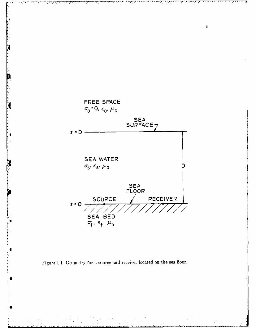
This work considers an electrically deep sea and calculates the electromagnetic

fields produced on the sea floor by three different sources co-located, along with the

receiver, on the sea floor, as illustrated in Fig. 1.1. The effects of the sea surface are

neglected because attenuation along the paths of propagation to and from the sea

surface is large. Both the sea and sea bed are assumed to be isotropic, homogeneous,

and time-invariant con ducting media separated by a plane interface. Computations

are restricted to frequencies in the ULF/ELF range, since it is only signals in these

. _ ....I. _ . - L . . . - : , _

3

bands that can propagate to significant distances through the conducting media

before becoming severely attenuated. The displacement current terms in both media

are neglected, and this assumption is well justified in these frequency ranges. It is

assumed that both media are nonmagnetic, with permeabilities equal to the free-

space permeability (p0 = 41r X 10- 7 H/m). The conductivity of the sea water is

o, = 4 S/rn and the conductivity of the sea bed varies.

The three sources considered are the vertical magnetic dipole (VMD), horizontal

electric dipole (HED), and infinite cable (IC). It is assumed that all the fields vary

with time as exp(it). The amplitudes of the field components for the VMD and

HED are obtained numerically through the techniques described by Bubenik [1977].

Three of the components are verified by computing the same components, using

expressions derived by Wait [1952, 1961]. The field comfy for the IC are

calculated from explicit expressions and numerical inter .c.Tn [Wait, 1953; Inan

et al., 1982]. Most of the data are presented in dimensionkess form by measuring all

distances in terms of the skin depth of the sea water b. defin. as

=(2/wpoa'.)"

where ,. is the angular frequency related to frequency f by the relation = 27rf.

The sea-bed conductivity is normalized to the sea-water conductivity by o =

al/a,, where a' is the normalized sea-bed conductivity. The skin depth in the sea

bed is related to the skin depth in sea water by 6f = 6,/v9, and the wavelengths

in both media are proportional to the skin depths because of the relation

X(,f) = 27r6(ef)

In conducting media, the field intensities variy with an exponential term e- d/i

(where d is the distance from the source) representing 55 dB/wavelength attenuation

[Hansen, 1963], and it is this attenuation that limits the range of the electromagnetic

signal. Figure 1.2 is a logarithmic plot of skin depth, wavelength, and exponential

attenuation in sea water as a function of frequency.

The numerical results obtained in this work should be useful in determining

an effective sea-bed conductivity in smooth regions of the sea floor. Stretches of

i . .. . ...- *---'- -- - - - - -

FREE SPACE(r -0 c 1

SEA

z D SURFACE7

SEA WATERO's. es. PLo D

SEA

SEA BED

Figure 1. 1. Geomnetry for a source and receiver located on the sea floor.

5

the abyssal plain in the western North Atlantic have been measured to be smooth

within 2 m over distances of 100 km [Pickard and Emery, 19821. It is also assumed

that the sea water shields the sea floor from atmospheric noise and, because the

region of interest is far from the shore, the possibility of atmospheric and power-line

noise propagating through the Earth's crust can be neglected. This is important

because atmospheric noise is especially strong in the ULF/ELF frequency range

[Liebermann, 1962; Soderberg, 1969]. The only other possible sources of noise are

thermal noise, motions of the sea water (assumed to be negligible), the internal

noise of the receiver, and, very speculatively, sources within the Earth's crust.

4i

6

105 102

10 o4 WAVELENGTH 10

zW 103 1

z 102 1- z

in 10 102 -IzC12 ATTENUATION

1 io- 310-2 10-1 1 10 102 103

FREQUENCY (HERTZ)

Figure 1.2. Skin depth, wavelength, and exponential attenuation in sea water witha conductivity of 4 S/rn (based on Figure A.3 by Kraichrnan [18761).

4

-. 7 -11 IL'- -

CHAPTER II. VERTICAL MAGNETIC DIPOLE

In this chapter we consider the electromagnetic fields produced by a small

current-carrying insulated wire loop located at the plane interface of two semi-

infinite dissipative media. As illustrated in Figure 2.1, the loop is taken to be at

the origin of a cylindrical coordinate system (p, 0, z), with its axis perpendicular to

the interface z=O (vertical magnetic dipole). The strength of the magnetic dipole is

IdA, where I is the amplitude of the loop current Icosw t and dA is the elementary

area of the loop.

A. Derivation of the Field Components

Following Wait [1052] to derive expressions for the field components, the mag-

netic vector potentials F, and F1 are first determined for the upper and lower

regions, respectively. They have only the following z-components:

F, - iwpoldAfI e-uz (

27r uf (2.1)

iwpoldA o° euz

fz - 2ir u + u 1 0(Xp)X dX (2.2)

where

22=iWjW, 72 = iW MO.;

Here, Jo(Xp) is the Bessel function of the first kind of zero order. The electric

and the magnetic fields are related to these potentials by

Ei = -Vx F,. (2.3)

Bi - -p 0 iFi + -.V '.Fi (2.4)

yielding

iwB i, = O2poz (2.5a)

7

(SEA WATER) *(PO, Z) SEA

z:O ~aE~/FLOORd

(SEA BED)

(a)

4Y

Z 0 PLANE ,* (p.zZO)

(b)

Figure 2. 1. Vertical magnetic dipole at the sea/sea-bed interface. (a) Side view, (b)

top view, showing azimuthal symmetry.

I

E =,- Op (2.5b)

iw2 - 2F (2.5c)

with Ei,- Bi,-" Ei, =0. The subscript i = a or f depending on whether the

fields are in the upper or lower region; therefore,

B,, = POI 0 u~ eU j(Xp)X2 dX (2.6a)2rff o us +tL,

E -i#poIdA e- (2.6b)E,, = 2f Jo u:-¥uJ(xP)x2 dx (.b

Bz poldA2_ 00 e-UOZ

-- fo u + ue J(XP)X3 dX. (2.6c)

When the observation point is on the z-axis (p = 0), there is only one nonzero

field component (the z-component of the magnetic field) along the z-axis,

B,- poIdA fo e0 C 3 d

2ff J U + Uf

which can also be expressed as

B,- I d A fo(u. - u 1 )e-uzX (2.7)2-y - -1) JO(.7

This expression can be rewritten in a dimensionless form by normalizing all dis-

tances by the skin depth of the sea water as

i A -- f)L f A' (2.8)i4ir( 1- o0 (l- l)

where

U1 + i2, U? = V\ 2 +i2o'

with z' - z/6,, X' = 6,X, and ao = o//.. Note that, when w=0, this magnetic

field component becomes

B.,, =poIdA47rz 3

€.

010

When the observation point is on the plane interface (z=0), the field com-

ponents in Eqs. (2.6) with the exponential term being unity can be expressed in a

dimensionless form as

- 6B., - poIdA f0 U1, J1 (X'P')X 2 dX' (2.9a)27r = u1 +U

=E, -idA 1 J (\').\ 2 V (2.9b)= =o u' + U,

-6

3 B od

'

B,Z = B.,,= PodA fo +u Jo(.\p')\'3 dX' (2.9c)

where p' = p/f. Following Wait[1952/, two of the the field components (E,, and

B,.,), have the following explicit expressions:

wiwpoIdA7r(- 2 .(- - )p4 [(3 + 3 -yfp + fp)e-',* - (3 + 3-1,p + yp2)e-"' (2.10)

and

B*,z "- podA [(9 + 9-yp + 4-y2p 2 + y p')e-,(*2127r(-12 - "y2)P 5 (2.11)

-(9 + 9gfp + 4 f p2 + -I'p')e- t "

S"The magnetic-field component B.,, and the electric-field component E.,O are zero

*at w=0, and the only nonzero field component B.,, at w=0 is

B6,, -poIdABz- 41rp3

B. Numerical Results

The three nonzero field components at the sea/sea-bed interface (z=0) are

numerically evaluated from the integral expressions in Eqs. (2.6), based on the

techniques described by Bubenik [19771. The dipole moment is set equal to unity

(1 Am 2) in these computations; the field amplitudes for any other dipole moment

can be obtained quite simply from the computed values by multiplying by the

appropriate dipole moment. Note that the electric field unit used in the data

presentation is the microvolt/meter and the magnetic field unit is the picotesla.

- --

I.I

The amplitudes of the field components are plotted in a dimensionless form for

sea-bed conductivities ranging from I to 0.001 (1, 0.3, 0.1, 0.03, 0.01, 0.003, and

0.001) times the conductivity of the sea water

Figure 2.2 shows the variations of the magnetic field components B and B2 ,

total magnetic field BT, and total electric field ET(= EO) as a function of the

receiver distance normalized by the skin depth of sea water. As indicated, the fields

are all presented in dimensionless form. The results are valid for all frequencies

in the range over which the assumptions made in the derivations are valid. The

actual field components can be obtained by substituting a numerical value for the

skin depth 6, at the frequency of interest. The observer distance ranges from 0.1

to 100 sea water skin depths. Note that both the vertical and horizontal axes are

logarithmic.

The ratios of the field components produced on the sea floor to the field com-

ponents produced in sea water of infinite extent (i.e., no sea floor) are plotted vs

normalized distance in Figure 2.3. The p-component of the magnetic field is zero

when there is no sea floor present and, as a result, no ratio curves are shown for

this component.

It is also possible to plot the field components in another dimensionless form

in which the horizontal axis shows the frequency variation for a certain receiver

distance. In Figure 2.4, the field components are parametric in terms of the actual

distance of the receiver, and the plots reveal the frequency variation of these

parametric components. Both axes are drawn with logarithmic scales. Again, the

actual field at any receiver distance can be derived from the curves that are shown

by substituting the value of the receiver distance.

The results of the numerical integration were verified by calculating two of the

field components EO and B,, using the explicit expressions in Eqs. (2.10) and (2.11).

Some of the low-frequency portions of the curves were also checked by comparing

their indicated field values with those obtained from the dc expressions for the field

components.

12

r 63IT -

0.3 0.001 0.001

;. lop

II

10-

10 -~' 0.001]

10-1 109 101 102 10-1 l0o 101 102

p/6. p/66

Figure 2.2. Variations in amplitudes of the electric and magnetic fields produced

on the sea floor by a vertical magnetic dipole as a function of distance. Note

that there are two components of the magnetic field, one parallel and the other

perpendicular to the sea/sea-bed interface, and only one component of the

electric field parallel to the interface. The dipole moment is unity.

S . . / '- i ,, " • " i, ,'. ' i

13

0.0010.

,lop

IB,.,IIIB,,o' = Il IBIrI/B0,.r(o' = 1)/

0.0010.001

102

=0.30.3

10-1 l o 10, 102 10-1 109 101 101

P/. p/6.

Figure 2.3. Variations in the electric and the magnetic fields produced on the sea* floor for an electrically conducting sea bed. The curves show the variation with

distance of the ratio of the electromagnetic fields on a sea floor to the fields inan infinitely deep sea water.

14

106 105

70 11

10 103 10

106 * 106

p'IB.,lAA

104 0.001

0.001 .0103 103

10-1 1 0 10t 101011 o,1

* Figure 2.4. Variations in the amplitudes of the electric and magnetic fields producedon the sea floor by a vertical magnetic dipole as a function of frequency. Thedipole moment is unity.

6

15

C. Summary

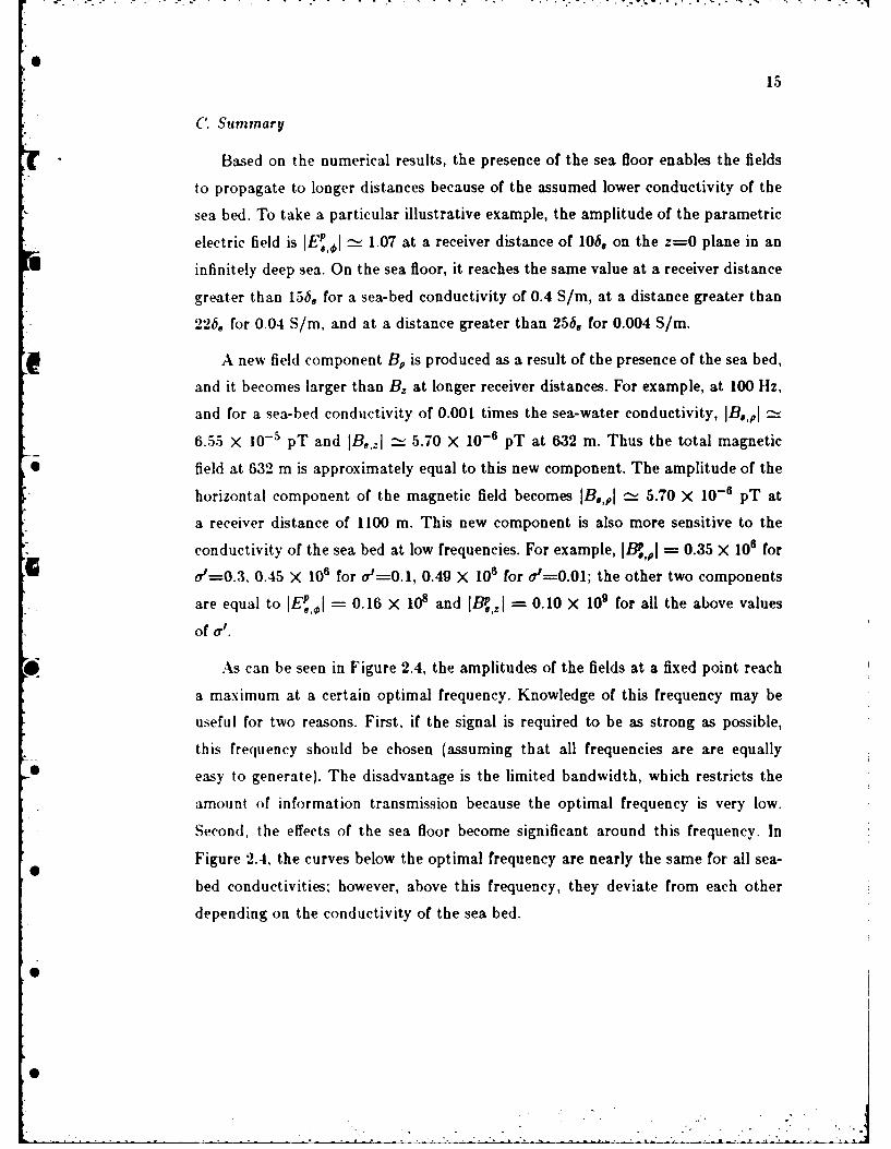
Based on the numerical results, the presence of the sea floor enables the fields

to propagate to longer distances because of the assumed lower conductivity of the

sea bed. To take a particular illustrative example, the amplitude of the parametric

electric field is JE,,I " 1.07 at a receiver distance of 106. on the z=0 plane in an

Uinfinitely deep sea. On the sea floor, it reaches the same value at a receiver distance

greater than 156, for a sea-bed conductivity of 0.4 S/m, at a distance greater than

226, for 0.04 S/m, and at a distance greater than 256. for 0.004 S/m.

A new field component Bp is produced as a result of the presence of the sea bed,

and it becomes larger than B, at longer receiver distances. For example, at 100 Hz,

and for a sea-bed conductivity of 0.001 times the sea-water conductivity, IB,pl :6.5.5 x 10-' pT and IB,,.I :-- 5.70 X 10-6 pT at 632 m. Thus the total magnetic

* field at 632 m is approximately equal to this new component. The amplitude of the

horizontal component of the magnetic field becomes IB.,l = 5.70 X 10-6 pT at

a receiver distance of 1100 m. This new component is also more sensitive to the

conductivity of the sea bed at low frequencies. For example, IB ,,,I = 0.35 X 106 for

u'=0.3, 0.45 X 10' for a'=0.1, 0.49 X 106 for o =0.01; the other two components

are equal to IE,,I = 0.16 X 108 and IB,ZI = 0.10 X 109 for all the above values

of eit.

*As can be seen in Figure 2.4, the amplitudes of the fields at a fixed point reach

a maximum at a certain optimal frequency. Knowledge of this frequency may be

useful for two reasons. First, if the signal is required to be as strong as possible,

this frequency should be chosen (assuming that all frequencies are are equally

easy to generate). The disadvantage is the limited bandwidth, which restricts the

amount of information transmission because the optimal frequency is very low.

Second, the effects of the sea floor become significant around this frequency. In

Figure 2.4, the curves below the optimal frequency are nearly the same for all sea-

bed conductivities; however, above this frequency, they deviate from each other

depending on the conductivity of the sea bed.

6

0"

"

CHAPTER I1. HORIZONTAL ELECTRIC DIPOLE

In this chapter we consider the electromagnetic fields produced by an elementary

current source located at the plane interface of two semi-infinite dissipative media.

As illustrated in Figure 3.1, the source is assumed to be located at the origin of

a cylindrical coordinate system (p, O, z), with the plane of separation of the two

media corresponding to z=O. The source is oriented along the z-axis (i.e., the 0=0

axis) parallel to the interface (horizontal electric dipole) and has an electric-dipole

strength of Idl, where I is the amplitude of the sinusoidal source current Icos(wt)

and dl is the elementary length of the source.


For convenience, the Hertz vector components are used instead of the field

components. Following Wait [1961], the rectangular components of the Hertz vector

in the upper medium are

, C . Jo(Xp)X dX (3.1a)

-.,.V = 0 (3.1b)

/H.z = cos 0 foa (u. - u,)e- ulz Jz(Xp)X 2 dX (3.1c)• A

whereIdl y

cos =X/p, p = X + y2

and the other terms are defined in Chapter II.

The electric and magnetic fields in the upper medium can be obtained using

the two vector expressions,

21-y~1. + VV.l (3.2Es = 'Ifn +('. I 3.2)

S 2!V X fl (3.3)

17

18

(SEA WATER) 0p:OZ) SE

(SEA BD)S(a

0'f ~ ~ - '- L(SEA~ BE) a

----- ---- IdL

(b)

Figure 3.1. Horizontal electric dipole located at the sea/sea-bed interface. (a) Sideview, (b) top view.

resulting in

=, + -(V.n) (3.4a)E,.p= -"'illp + Op

E.,= + 1(V.116) (3.4b)

S p O4

E.,z + O(V rI.) (3.4c)

= (iOH. e,4-)- (3.4d)

917o,.p i9T.,)B I 4 -W( '9 H6,p(3.4e)

B!,z " 17,, + -f Op ) (3.4f)

where 1,,p, h, , , and H/,, are the components in the upper medium in cylindrical

coordinates. The divergence of the Hertz vector is

v. C -- cos, -fo e J(Xp)X dX (3.5)

Based on Eqs. (3.4) the field components can be obtained in the following form:

= CeYco 00 USUCUzJ I (foo u 6ufe dx)]E..,P C."C 2Cos i[- f f JoX d + (A J, d

00cs -U tf Jl dX (3.6a)

E.,i+ JoX dX + 0 J dA

-- ef O +U J, A) (3.6b)

[ o fO U e -u

E,,z CO'IN Cos fo A- J(kd3.6c)

20

2 00 u6e-U*z 1 00 uee-ulzBP- _ sin -fJoXd J+ -+ JidXj2W 0.z us + uf P0u, + u/

-27 10 J, dX (3.6d)

0 0 00-uzI f use-uez1 d-C7ol JoX dX + -- Ji dXB 6 i o s 01 Y p P 0 u , + u f

( 100 ufeu uo J, dX)] (3.6e)

B,, J sin dX (3.6f)W i-- u-s + Uf J 2

where the argument of the Bessel functions J0 and J1 are the same as Eqs. (3.1).

The field components can also be written in a dimensionless form as follows:

E8,(p,¢z) a (3.7a)

SB ,(p,,,z) -62B.,{,,z ) (3.7b)

Note that the terms on the left-hand side are independent of receiver distance so

that, after the parametric fields are numerically determined, they can be useful for

all frequencies in the valid frequency range.

Equations (3.6) can be simplified by considering two observer locations. The

first is along the z-axis (p = 0) where the only nonzero field components are the

x-component of the electric field E,, and the y-component of the magnetic field

* B.,y given by

' f IA X dX + , XdX (3.8a)E.,Z- 2 a 0us + uf

__ 1 2 f 00 U 0 0 eUZB - 6 0 X dX + f X dX (3.Sb)'Y i~wu, + uf

which become

-Idi* E.,z = 2ir(o. + uf)z3 (3.9a)

-

21

B.,1 __ (3.9b)

The second observer is located at the interface separating the two media (z=O),

where the field components are the same as in Eqs. (3.6) but without e-U in all

the integrals. Wait [1961] derived an explicit expression for the z-component of the

magnetic field B,, in the following form:

poldl sin +-22ej Y

B,2 = 2 o 4 [(3 + 3-If + p2)e- tp - (3 + 3-y.p + 2p2)e-," (3.10)2r(y2 - 2)1(4 ~ fp

Three of these field components E.,,, B,,,, and B*, are zero, for the dc case, and

the other three simplify to

IdN cos ( 1E 7r " (a. + orf)p 3 (31a

Idi sin 4E,,O N si 0 -(3.116b)2,, "-r(o,. + orf)p3 3lb

B,,2 - poldl sin 4 (3.1lc)41rp 2 31)


The electric and magnetic field components at the sea-floor interface (z=0)

are numerically evaluated from the integral expressions for two azimuthal angles

-= 00 and 4- 900 , using the techniques described by Bubenik [1977]. The field

components at any arbitrary 4 can be obtained from these results by multiplying

them by either sin 4 or cos 4. The electric dipole moment is set equal to unity (1

Am), and the field components for any arbitrary dipole moment can be determined

by multiplying these results by the dipole moment; the units of the electric and

magnetic fields are in microvolts/meter and picoteslas. The results are plotted in

a dimensionless form for various sea-bed conductivities ranging from 1 to 0.001 (1,

0.3, 0.1, 0.03, 0.01, 0.003, 0.001) multiplied by the sea-water conductivity. The axes

are logarithmic.

The amplitudes of the nonzero field components E,,,, B.,,, and E.,, and the

total electric field E,,T are plotted vs distance in terms of the skin depth of sea

i ~ I

22

water for an azimuthai angle of 4, = 00, as illustrated in Figure 3.2. Figure 3.3

plots the variations of the amplitudes of the nonzero field components B,,,, E,,O,

and B,, and the total magnetic field B,,T when 4, = g0 . All the results can be

converted to the real field values for any frequency by substituting the numerical

value of the skin depth b. at that frequency and the conductivity a, of the sea

water. The receiver distance varies from 0.1 to 100 sea water skin depths.

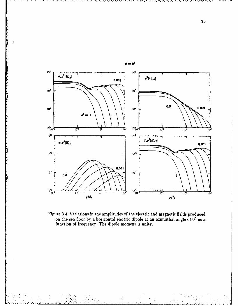
The numerical results for the field components in the alternate dimensionless

form can be obtained by holding the distance of the observer constant and varying

the frequency, as demonstrated in Figures 3.4 and 3.5, where the increase in the

horizontal axis shows the rise in frequency. The actual field values for any arbitrary

receiver distanoe p can be calculated from these curves by substituting the numerical

value of p in the parametric expressions.

-* The z-component of the magnetic field B,,, was also calculated from the explicit

expression in Eq. (3.10), and the results were used to verify those obtained by the

numerical integration of B.,,. The dc expressions for some of the field components

were also used to check the lower frequency portion of the curves.

C. Summary

The ranges of the electromagnetic signals tend to increase as a result of the

lower conductivity of the sea bed, as indicated by all the numerical results. For

example, when the sea-bed conductivity is 0.01 times the sea-water conductivity,

the increase is approximately a factor of 105 at distances of 10 to 20 skin depths.

The new field components produced by the existence of the sea floor are the p-

and O-components of the magnetic field B,,, and B,,o and the z-component of the

electric field E.,,. The new magnetic field components B.,,, and B,, become larger

than the z-component of the magnetic field B,, at longer distances, which results

in a greater total magnetic field. The new component of the electric field does not

have this property; however, because of its sensitivity to sea-bed conductivity even

at low frequencies, it may have useful applications in sea-bed prospecting.

Figures 3.4 and 3.5 show the variations of the fields with frequency. As can be

seen, all of the field components are sensitive to the conductivity of the sea bed

6

-00

623

.103! 1.

,o, .o,_ - i \\ ooo 1

II 0.001 0.001

o~=1 0.31

10-3 5

F .

10o3 -,j\\ o~,-

U -,

F10-1I 160 101 10" 10-1I 10o 101 0

I-- 10

i Figure 3.2. Variations in the amplitudes of the electric and magnetic fields produced

• on the sea floor by a horizontal electric dipole at an azimuthal angle of 0°D as a

I! function of distance. Note that there are two components of the electric field, one

parallel and the other perpendicular to the sea floor, and only one component

of the magnetic field, directed parallel to the floor. The dipole moment is unity.

0."~

24

=90P

1011

V 0.001A

E 0.001 -

0.3

io-3

10-3

10 - 1___0_____1__10;_____1_____ ____1__102

6~IB., 6~IBPAP-

4 Fgue .3 Vrit isInLheamliuds f heelctic ndmaneicfild podceonth sa lorbya oizntl lcticdioe t n zmuha age f 00aa fuctin o ditanc. Nte hatther ar tw coponets f te mgneifild oe aalelan teoterpepndcuartote eaflor ndony ncompnen ofthe lecricfiel, dreced pralel o th flor.The ipoe mmenis unity

25

106 =06

0.00Ip~l,,,I

0.0.3

04 0 0.001

0 103

lot 102E10

10 1 to

0.3a

Figure 3.4. Variations in the amplitudes of the electric and magnetic fields producedon the sea floor by a horizontal electric dipole at an azimuthal angle of 00 as afunction of frequency. The dipole moment is unity.

26

105 10

l104104

102 1010 71015 108

p'I~h~aIIB,TI

105 10

0.001

I10310 U10,I 1 601 102 r

Figure 3.5. Variations in the amplitudes of the electric and magnetic fields producedon the sea floor by a horizontal electric dipole at an azimuthal angle of 900 asa function of frequency. The dipole moment is taken to be unity.

0

27

at low frequencies except for the vertical component of the magnetic field. The

vertical component of the electric field is interesting because it is highly sensitive to

sea-bed conductivity at low frequencies and has an optimal frequency that is also

sensitive to the same conductivity, Unlike the magnetic field components B.,, and

B..O produced at the sea floor, this component is not large at long distances and,

as a result, it does not contribute to the total electric field.

F.

S

0

[ - -,. .1

.7 7 - - -Q W4 7

CHAPTER IV. INFINITE CABLE

In this chapter we consider the electromagnetic fields produced by a straight

current-carrying insulated cable of infinite length lying at the plane interface of

two conducting media-in our case the interface between the sea and the sea bed.

We use the term "infinite" in a relative sense: if the length of the cable is much

greater than all the other relevant linear dimensions, it is known as an "infinite"

* -cable. It is assumed to carry an equally distributed alternating current Icoswt at a

given instant of time, and this assumption is justified at sufficiently low frequencies

[Wait, 1952a; Sunde, 1968]. The cable is oriented along the x-axis, and the plane

interface of the two media is z=O. Figure 4.1 shows the geometry in the y, z plane;

everything is invariant in the x-direction and the direction of the current is taken

to be out of the page at t=O.


The Hertz vector components in the upper medium for an RED lying at z=0,

oriented along the x-axis, and located on the x-axis at z = I are the same as in Eq.

(3.1) with x replaced by x - I. For an infinite cable, the Hertz vector components

can. be derived by integrating the components of the Hertz vector for an -lED from

I = -o to I = oo, which results in

M coo e-U@z

• / =,' -C J ] J)(Xp) X dX dd (4.1a)

K ~il" =0 (.b

HeZ C a LI r f-ueu Jo(Xp)X dX dl 4 cwhere

and all the other quantities were defined in Chapter M. The partial derivative a/cx

,can be replaced by -a/W1 to yield

//17,z -- 0

29

0 .

30

(SEA WATER) I~:~) SEA

O~(Y 0),.L(SE BED) /

i~ Fiur Z.1 Iiiecbl oae a h e/sabditrceNoeheym tywith~~ repc to th N-axTsE

CAL

aI.6 1

(SABD

31

Because the divergence of the Hertz vector is also zero, the only nonzero vector

component is the x-component. By using the integral [Sunde, 1968]

f Jo( p) dl - co $(XY)

the expression for this component can be simplified to

00 e- U O

z

4/,= 2C" J( U-+Uf cos(Xy) dX (4.2)

The electric and magnetic field components can be derived from the Hertz vector

via Eqs. (3.2) and (3.3) as

E,z - w- ( 00 e Uf cos(Xy) dX (4.3a)

7. Jo us + u 1

B6 ' 0 o ue-U*z cos(Xy)dX (4.3b)B 7~ -- us + u r

pol PoI Xe- sin Xy)dX (4.3c)

where B8,, = E,,y 2 = 0.

As in Chapters II and m11, two receiver positions are considered which, to some

extent, will simplify the above expressions. When the receiver is located along the

line perpendicular to the interface and passes through the infinite cable (y=O),

B,z-=O and the other two field components become

-1 U~jOI00e-UoZ

-- us - dX (4.4a)7 Jo us + U 1

, r -Ou.+t -f dX(4.46)

These expressions can be further simplified by multiplying the numerator anddenominator of the integrands by u, - u; and following an approach similar to

" 6" ... .

32

that used by Wait and Spies [19711; then,

E,,X - (V-) - Ko(-y.z)- ufe- - °" dXj (4.5a)= ' -y2 49[2 10

B,,y -r-OI _ r) -z2hKo(z) -fo ufe-u'z dX (4.5b)

Note that Ko(- 8 z) is the modified Bessel function of the second kind of zero order

and with complex argument. In the dc case, the above two components can be

written

P zE 0, B,'- = 21rz

* When the receiver is located at the interface z=O, the field components can be

written in dimensionless form as

7ror, 6 200 up ZrE766e f* e- '*'EZ- E. - -,im i2 J e- + u- cos(X'y') dX' (4.6a)

v , /o use-"'B,- Pol B,,y- z.-ol * u + ' (4.6b)

f2 r6. f00 Xle-uez'(.cP. B.,z = lirm Vf2o sin(Vy') d' (4.6c)

* where

"us' \/XP + i2, U = V(/ + i2or'

and z' . z/6., y = y/6., V = X6., and a' = a /&,. Wait [1953, 1962] derived

explicit expressions for the horizontal electric field component E.,, and the vertical

magnetic field component B,,, as

E,,Z -2 W(7 - [, y K I( - y ) -- 7f yK(,7fy)] (4.7)

- [Cy:.K-- ,

0 . . - . .. . .. , i . .. . / . . :

33

Bo'Z -= po [2-. yKI(-y) + -y 2y 2Ko(-I.y)f3 -- 12)y3

-1 2(4.8)

-21f yKI(-fy) - Vy 2 Ko(yfly)]

where, again, K0 and K, are the modified Bessel functions of the second kind

of order zero and one with complex arguments. The horizontal component of the

magnetic field B,.y does not have an explicit expression. When w=O, both E,,, and

B,. become zero and the vertical magnetic field component simplifies to

4., = POI


This section presents the numerical data for the electric and magnetic field

components at the interface of the two conducting media. Two of these components,

E,2 and B,, have explicit expressions [Eqs. (4.7) and (4.8)] that can be expressed in

terms of Kelvin functions [Young and Kirk, 1964] and their derivatives. After some

(algebraic manipulations, their amplitudes can be written in dimensionless form as

EI E s,.- 2 [(c- Rc2 )2 +(di - Rd2)211/2 (4.9)

~ E.~j (1 R2)ck[(1 i

* and

V~, '2ir6 8 IB6,I=l (1 2--= Pol1 R2)o2 [(a6 (a1 - R2a2 ) - 2(d1 - Rd2))2)2

(4.10)

* +(a.(bi - R 2b2 ) + 2(cl - Rc2))2 1/2

where

a, =keroac, a2 - keroa f

b1 =kei0a, b2 = keioa f

c, =keroo, C2 - ker'10

d =keioao, d2 = kei'oaf

"- '•w - -.- - --- -

34

and

Or a6 V'2_V, cif=Ra, R 2 =&= Of/0,

where a6 and af are defined as the induction numbers in the sea water and sea

bed respectively [Coggon and Morrison, 1970]. The above expressions for E,,, and

B,., can be evaluated numerically by using tables of Kelvin functions and their

derivatives [Lowell, 1959].

The other nonzero component at the interface is the horizontal magnetic field

component B,,,, and it can be computed only by numerical integration. The ex-

pression for it [Eq. (4.6b)] can be divided into two parts,

BP, _ m U0 cos(X'y) dX'- li Vrf 0 U.eUZ cos(X') dX= U' + U os' -0 M.. U + Ufe

f

Two factors must be determined for numerical integration. The first is X' ". It is

assumed that the effective conductivity of the sea floor is smaller than that of seawater (a' < 1). The value for )', is chosen such that X 2 2 and, if this

constraint is satisfied, both u' and u , can be approximated as

f

for X > ,,a .. Based on this approximation, the second integral above can be

replaced by an explicit term yielding

,= V f u. cos(X'y) dU1+ + U(XV2-y/(4.11)

Similarly the integral expression for the vertical component of the magnetic field

[Eq. (4.6c)] can be written as

B )". X' cos(XMY9) (4.12),zV = 2Ju sin(X'y) dX' + (4.12)

The above integrands can be separated into their real and imaginary parts and thus

numerically integrated as real integrals. The data for the field components can then

be obtained by recombining these terms according to Eqs. (4.11) and (4.12).

• .*. • -, . ,, . . . . , .- -. ,..-- - - - - - -,,-- - - -.-- - - - - - -.--- r, J . . I

35

The second factor that must be determined is the method of integration. Both

integrands are well-behaved functions except for the cosine or sine term that may

oscillate rapidly at greater distances than the skin depth of the sea water [Hermance

and Peltier, 1970]. Two techniques of numerical integration, Weddle's rule [Computation

Laboratory of Harvard University, 1949] and Filon's method [Tranter, 1956], were

used. Provided the integration interval is made small enough, both techniques

produce sufficiently accurate results.

The computations can be verified in several ways. The first one is to compare

the results of the two integration techniques. The second is to compare the results

obtained for B,, through numerical integration using Eq. (4.12) to the results

obtained for the same component using Eq. (4.10) and tables of Kelvin functions.

The third is to check the lower and higher frequency regions by approximate

expressions for these regions.

The left hand panels in Figures 4.2, 4.3, 4.4, and the single panel in Figure

4.5 show the variations in the parametric amplitudes of the three nonzero field

components E, , B,,, and BP, and the total magnetic field BPT with the induction

number of sea water a,. Note that the parametric terms 7ro,62/I and ,/'27r6./poI

appearing on the left hand side depend on frequency f and not on receiver distance

y [see Eqs. (4.6)]. These curves can be used for any frequency in the valid frequency

range. The horizontal axis indicates the perpendicular distance of the receiver from

the axis of the cable along the sea floor in terms of skin depths of sea water. Each

curve corresponds to a different value of R (R = r"f,/a); R takes the values of

0.01, 0.03, 0.1, 0.3, and 1 except for the BP,y component which is zero when R=1

(no sea floor). Both axes are plotted on a logarithmic scale, and the units are in

volts/meter and teslas.

The right hand panels in Figures 4.2 and 4.4 show the variations of the amplitude

ratio of E,,, and B,, produced on the sea floor to those produced in a sea of infinite

depth as a function of distance. The horizontal magnetic field component B,,, is zero

in the absence of the sea floor. The second panel in Figure 4.3 plots the variation of

the ratio of the amplitude of B.,y to the amplitude of B,, as a function of distance.

36

-- - - ft --.

.. ......R 0.1 b

-~'b

4b

- /7

Figure 4.2. Variation with horizontal distance of (1) the amplitude of the electricfield produced on the sea floor by an infinite cable (left panel) and (2) of the ratiocurves illustrating the changes produced in the electric field by the presence ofan electrically conducting sea bed (right). Each curve corresponds to a differentsea-bed conductivity. The curves in the right hand panel show the ratio of theelectric field at the sea floor to the electric field in an infinitely deep sea.

37

.... a.. .. :

.. .. .. ... .

C6.0

corsodta dfet sa-e dutity.o

I °38

',b.

16,N,. id-i a, i 0 d

Fiur 4.4. 'Vrato wthoiotldsac.f()te mltd ftevri

• .~ . . . . .R - e . $

--- / /- //

S' ". .. ;

*"o"'A , -€,'"o o .. . s . . .

• cal component of the magnetic produced on the sea floor by an infinite cable" (left panel) and (2) of the ratio curves illustrating the changes in the vertical• component of the magnetic field produced by the presence of an electrically• conducting sea bed (right). Each curve corresponds to a different sea-bed con-,. ductivity. The curves in the right hand panel show the ratio of the verticalcomponent of the magnetic field produced on the sea floor to the same com-~ponent in an infinitely deep sea.

- I

,-- :. .. .-.-" .- .. . -..- 2

b

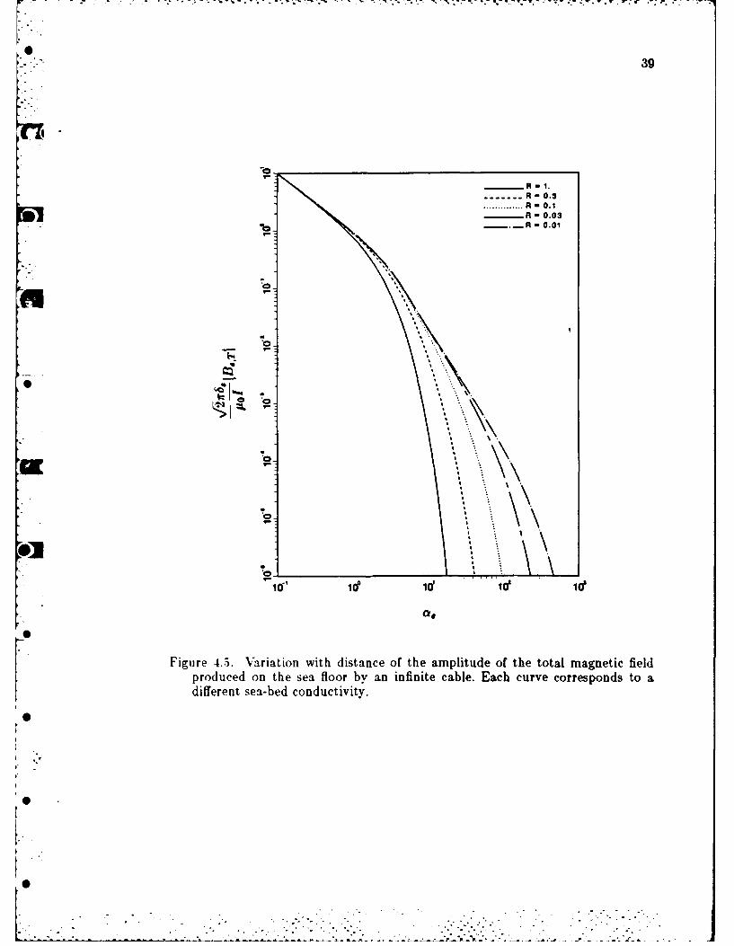
39

R

R" 1.

------- R-0.3............. R 0.1

R - 0.03-.. R -0.01

0*

0a

''S

00

0*N

Fiue-..Vrainwt itneo h mltd ftettlmgei ilprouce ontesaforb nifnt ,abeahcrecrepnst

diffren seabedcondctiity

0

0.

0 \\

40

- U-.. . . 0-.3

00.'

b - 0,3o~o

FA .2 '.

I=fnt c100e cAryn lnatraigcretwtb mltd f10 n

-a

a frequency of I Hz. Each curve corresponds to a different sea-bed conductivity.

"d .*C." "" " " " -

41

0.0

i " 0=1000 A

f -

2'b.

*00

0-

DISTANCE (METER) DISTANCE (METER)

Figure 4.7. Variation with horizontal distance of the amplitudes of the total electricand magnetic fields produced on the sea floor by an infinite cable carrying analternating current with an amplitude of 1000 A and a frequency of 1 Hz. Eachcurve corresponds to a different sea-bed conductivity.

42

In Figures 4.6 and 4.7, the real amplitudes of the field components E.,., B.,1,

B, and the total magnetic field B,, are plotted vs distance for an alternating cur-

rent source with an amplitude of 1000 A and a frequency of 1 Hz for the above sea-

floor conductivities. The units of electric and magnetic fields are millivolts/meter

and picotesla, and distance is in meters.

The above results can be plotted in another parametric form in which the

amplitude of the field components is written as

-EP.,.I = rIE,.I (4.13a)

l ,,lB

B'- , (4.13b)

Here, the terms on the left hand side are not functions of frequency but, instead, are

functions of receiver distance y. Figures 4.8 and 4.9 plot the variations of the field

components in Eqs. (4.13), and the horizontal axis shows the variation in frequency.

Note that each curve now corresponds to a different sea-floor conductivity; again,

there is no horizontal magnetic field component for R=1.

C. Summary

All three field components produced at the interface can propagate farther when

e a sea floor is present than can those produced in the absence of a sea floor because

of the assumed lower conductivity of the sea bed. The increase in range becomes

significant at greater distances. For example, when f=1 Hz, the amplitude of the

horizontal component of the electric field E, becomes 1 nV/m at a distance of

y = 3 km for a'=1 (infinitely deep sea), y = 18 km for 01=10 - 2, and y 90 km

for a,=10- 4.At 90 km, the source cable must be much longer for it to be an infinite

cable; for example, if it is ten times longer (900 km), a uniform current distribution

is still a good assumption at 1 Hz [Inan et al., 1983J.

The new magnetic field component B,,1 is parallel to the interface and perpen-

dicular to the axis of the source. It is negligible when compared to the vertical

component B,,. near the cable; however, it becomes comparable to and larger than

I

-~~...............................".......:i:-.:: .:-::i-:: - ::.i....."

43

.......... R .01

-r Id IdI I o

as Of

Figure ~ ~I 4..Vrain\nteapiue fth oa lcrcfedadhrzna

co poen oftemge i il rdcdo h e forb nifnt al

asa untin f reuec. ac crv crrspnd o dffret eabe cn

ducivty

44

5b

R - 0.03

+- .. a-

a 2

2A

t1 0 - d

lit-

Figure 4.9. Variations in the amplitudes of the vertical component of the magneticfield and the total magnetic field produced on the sea floor by an infinitecable as a function of frequency. Each curve corresponds to a different sea-bedconductivity.

4

45

Hz, and o' = 0.01, the amplitudes of the horizontal and vertical magnetic field

components would be IB,,yI -- 0.70 x 106 pT and IB,,ZI = 0.20 X 108 pT at 10 m,

0.57 x 106 and 0.19 x 107 pT at 100 m, and 0.68 X 105 and 0.30 X 105 pT at 1

km. The new component is also more sensitive to the conductivity of the sea bed

than are the other two field components at lower frequencies.

The horizontal components of the magnetic and electric fields are zero when

w=0. They also have optimal frequencies, as observed in Figure 4.8. For example,

at a distance of 1 km, the electric field component has an optimal frequency of

approximately 0.15 Hz in an infinitely deep sea [Inan et al., 1983).

0.

0"

0[

0

0

CHAPTER V. CONCLUSIONS AND RECOMMENDATIONS

A. Conclusions,

This investigation has concentrated on the electromagnetic fields produced

along the sea/sea-bed interface (considered to be a plane boundary between two

U semi-infinite conducting media) by several different harmonic sources: a vertical

magnetic dipole, a horizontal electric dipole, and an infinite cable. New expressions

and numerical results have been obtained for the electromagnetic fields produced by

these sources. The displacement current terms in both media have been neglected,

4 which is valid for frequencies of less than 100 kHz. The results have been expressed

in two dimensionless forms that make them useful for all frequencies and receiver

distances in the above frequency range. These new results can be summarized as

follows.

1) 'Vertical magnetic dipole: the three nonzero field components at the sea/sea-

bed interface are the horizontal magnetic field component in the p-direction, the

horizontal electric field component in the 0-direction, and the vertical magnetic

field component in the z-direction. The first is a new component (compared with

what would be produced by the same source in a sea of infinite extent under

otherwise identical conditions) that can be useful because it (1) becomes larger

than the vertical magnetic field component at greater receiver distances, (2) has

* an optimal frequency at which the amplitude of the field has a maximum, and (3)

is more sensitive to the conductivity of the sea bed than the other components

at, low frequencies. The horizontal electric dipole also has an optimal frequency.

Both horizontal components are zero in the dc case and become more sensitive to

6 the conductivity of the sea bed above the optimal frequency than does the vertical

component of the magnetic field, which is nonzero in the dc case.

2) Horizontal electric dipole: all six field components are nonzero on the sea

* ~floor interface. The two azimuthal angles considered are 0 = 00 and v0 = 000.

At o = 00, the three nonzero field components are the horizontal component of

the electric field along the axis of the source, the horizontal component of the

magnetic field perpendicular to the axis of the source, and the vertical component

*of the electric field perpendicular to the sea floor. Both the horizontal magnetic

47

48

field component and the vertical electric field component are the result of the

sea/sea-bed interface. The horizontal and especially the vertical component of

the electric field are sensitive to the conductivity of the sea bed even at very

low frequencies. Another interesting feature is that it has an optimal frequency

which, unlike other components, is also very sensitive to the conductivity of the sea

U bed. At 0 = 900, the three nonzero field components aie the horizontal magnetic

field component perpendicular to the axis of the source, the horizontal electric

field component parallel to the axis of the source, and the vertical magnetic field

component perpendicular to the sea floor. Only the horizontal component of the

magnetic field is produced as a result of the sea/sea-bed interface; it becomes

larger than the vertical component at greater receiver distances, is sensitive to the

conductivity of the sea bed at low frequencies, and is zero at w=0, The horizontal

component of the electric field at - 900 is also sensitive to the conductivity of

the sea bed at low frequencies.

3) Infinite cable: the three nonzero field components at the interface are the

horizontal electric field component aligned with the axis of the source, the horizontal

magnetic field component perpendicular to the axis of the source, and the vertical

magnetic field component perpendicular to the sea floor. The horizontal component

of the magnetic field becomes larger than the vertical component at large receiver

distances, has an optimal frequency, it is sensitive to the conductivity of the sea bed

at low frequencies, and is zero at w=0. The horizontal component of the electric

field is also zero at w=0 and has an optimal frequency. The vertical component of

the magnetic field is nonzero even when w-0.

* The electromagnetic signals produced along the sea floor can propagate farther

because of the assumed lower conductivity of the sea bed. Also, new field com-

ponents are produced as a result of the sea/sea-bed interface and, because they

are comparable to and even larger than the components existing in the infinitely

deep sea, they produce larger total fields. For example, for an infinite cable carrying

alternating current with an amplitude of 1000 A and a frequency of 1 Hz, for a sea-

bed conductivity of I S/m, the amplitude of the vertical component of the magnetic

field is approximately 0.47 pT at a receiver distance of 5 km. The amplitude of the

horizontal component of the magnetic field at 5 km is approximately 0.75 pT, which

49

increases the amplitude of the total magnetic field to roughly 0.88 pT. The new field

components are also sensitive to the conductivity of the sea bed; for example, in

the case an infinite cable, the parametric amplitude of the horizontal the magnetic

dipole is 0.37, 0.50, and 0.61 for o = 0.25, 0.09, and 0.01 at a sea-water induction

number of a. = 0.1, whereas the parametric amplitudes of the vertical magnetic

g dipole at the same sea-bed conductivities and sea-water induction number are 10.

Even this component becomes less sensitive to sea-bed conductivity, however, as

the conductivity is reduced. The optimal frequency may have some applications

for communicating at short ranges and for sea-bed prospecting. For example, for a

C vertical magnetic dipole, the optimal frequency occurs when the receiver distance is

3 to 4 times the skin depth of sea water and the maximum value of the amplitudes

of the horizontal magnetic and electric fields are sensitive to the conductivity of

the sea bed at low sea-bed conductivities.

B. Applications

An active experiment has been conducted on the sea floor in the vicinity of

the East Pacific Rise to investigate the conductivity of the sea bed by analyzing

the measured data [Young and Cox, 1081]. The numerical results that have been

obtained in Chapters H,,IHI, and IV could be applied to investigate the effective

condIuctivity of the sea bed (assumed to be homogeneous). Two methods can be

used. One is to keep the frequency of the source constant and to vary the observation

distance along the interface; however, most of the field components become sensitive

to the effective conductivity of the sea bed at distances greater than a skin depth of

sea water. The other is to hold the location of the observer constant at the interface

and to vary the frequency of the source; in this case the optimal frequency may

yield useful information.

Another application is the use of electromagnetic signals for undersea com-

* munication. The range of communication with submersibles in the deep parts of

the ocean is limited because of the high conductivity of the sea water. The sea

bed has an effective conductivity smaller than that of sea water and, as a result, it

may provide a new path for the signals along which there will be less attenuation

compared to a signal propagating directly through sea water; longer ranges can be

achieved before the signal becomes weak and cannot be detected because of external

and internal receiver noise. The sea bed is also a conducting medium and exponen-

tial attenuation is still significantly large at high frequencies; therefore, operating

frequencies must be low enough to reach long ranges. This limits the bandwidth,

and information cannot be transferred at a high data rate.

New field components at the sea/sea-bed interface will increase the ranges of

communication. For an infinite cable carrying an alternating current of 1000 A at

1 Hz, and assuming the minimum measurable magnetic field to be 0.1 pT, the field

on the sea floor can be detected over a range of approximately 4 km before its

amplitude drops below 0.1 pT. The amplitudes of the new horizontal component

and the vertical component of the magnetic field along the interface are 0.24 and

0.09 pT at a receiver distance of 8 km for an effective sea bed-conductivity of 0.4

S/rn, thus producing a total magnetic field of 0.26 pT. If the sea-bed conductivity

is 0.04 S/in, then the two field components are 0.27 and 0.03 pT at a receiver

distance of 20 kin, and the total magnetic field becomes 0.27 pT as a result of this

new component. These two components are about 0.39 X 103 and 0.22 X 102 pT at

20 km for a sea-bed conductivity of 0.004 S/in. These examples indicate that the

range of electromagnetic fields along the sea floor increases significantly before their

amplitudes drop below the minimum measurable field value.

Arrays of long cables located on the sea floor can achieve longer communication

ranges [mnan et al., 1982]. The phases of the currents in each cable can be adjusted

to produce a maximum field amplitude at the receiver, which makes communication

possible over a much larger area. The separation distance of the cables depends on

the amplitudes of the current, frequency, conductivity of the sea bed, sensitivity

of the receiver, and background noise. With a series array of cables, each carrying

an alternating current of amplitude 1000 A and frequency 1 Hz and separated

from each other by 30 skin depths, the magnetic field produced at a point midway

between the two cables would be approximately 4 X 102/6. or 1.6 pT in an infinitely

deep sea; on a sea bed with af =0.04 S/in this field would be 4.6 X I pT, which

indicates that the cables could be moved apart from a spacing of 306, to 1406, while

still yielding the same field at the center point. Large amounts of power will be lost

due to resistive beating in both cases, however, as the source current flows in both

the long cables and surrounding conducting media. The advantage of this system

is a less noisy environment in which the electromagnetic signals propagate, since

there is significant shielding of atmospheric noise by the large bulk of sea water

[Mott and Biggs, 19631.

C. Recommendations

Throughout this investigation, it has been assumed that the sea bed is a homo-

geneous medium; however, it actually contains layers of sediment with different

properties. This work could be extended to two or more layers. For example, in the

two-layer bed in Figure 5. 1, the first layer has a conductivity of 0pf and extends

from z=O to z=-h and the second has a conductivity Of aI2 and extends from

z=,-h to z=-oo. Both the source and receiver are located at the sea/sea-bed

interface. The conductivity of the upper layer is larger than that of the lower layer.

For receiver distances smaller than the depth of the first layer, the effects of the

low-conductivity layer should not be very significant. As receiver distances become

larger than the depth of the first layer, however, the signal that follows the down-

under-up mode will be much stronger than the signal that directly propagates from

the source to the receiver using the sea/sea-bed boundary, and the lower layer will

be important. This means that, depending on the location of the observer, the signal

at the receiver will carry information about the properties of different layers of the

sea bed.

The length of the straight current-carrying cable source was assumed to be

infinite. This is a good assumption for a receiver located in the vicinity of the cable

(i.e., the perpendicular distance to the receiver is much smaller than the length of

the cable) and not close to the ends of the cable. A uniform current distribution

along the cable was also assumed. Although this is not true in an infinite cable,

the fields produced at the receiver will be the result of the middle portion of the

cable because the contribution from the portions toward the ends (not necessarily

carrying the same current) will be negligible. As the receiver distance increases,

however, a longer portion of the cable must be considered and the uniform-current

assumption may no longer be valid. One extension of this work would be to calculate

the fields produced on the sea floor by a straight current-carrying insulated cable

of finite length.

52

SEA WATER o-s

SEAFLOOR

SOURCE RECEIVER

>iUPPER LAYER-OF THE SEA BED fi

LOWER LAYEROF THE SEA BED

Figure 5.1. Geometry for a sea bed containing two conducting layers..

I

I

q-

53

In practice, it may not be possible to locate the receiver precisely at the interface.

Another extension would be to place the receiver some distance above the sea/sea-

bed interface and then calculate the fields for this configuration. The integrals for

the field expressions will then require an additional exponential term e- u' because

of the attenuation of the signal as it propagates the vertical distance between the

source and receiver in the sea water. As a result of this attenuation, the signals at

some vertical distance away from the source will be smaller than on the sea floor.

REFERENCES

Bannister, P. R., "Determination of the electrical conductivity of the sea bed in shallow

waters," Geophysics, 88, 995-1003, 1988a.

Bannister, P. R., "Determination of the electrical conductivity of the sea bed in shallowwaters," Geophysics, 88, 995-1003, 1968b.

Bannister, P. R., and R. L. Dube, Numerical results for modified image theory quasi-sta. ic

range subsurface-to-subsurface and subsurface-to-air propagation equations, Tech. Rep.5775, 30 pp., Naval Underwater Systems Center, New London, Connecticut, 1977.

Banos, A., Dipole Radiation in the Presence of a Conducting Half Space, 245 pp., Pergamon

Press, New York, 1966.Brock-Nannestad, L., "Determination of the electrical conductivity of the seabed in shallow

waters with varying conductivity profile," Electron. Letters, 1, 274-278, 1985.

Bubenik, D. M., "A practical method for the numerical evaluation of Sommerfeld Integrals,"

IEEE Trans. Ant. Prop., AP-25, 904-906, 1977.Bubenik, D. M., and A. C. Fraser-Smith, "ULF/ELF electromagnetic fields generated in a

sea of finite depth by a submerged vertically-directed harmonic magnetic dipole," Radio

Sci., 18, 1011-1020, 1978.Burrows, C. R., "Radio communication within the earth's crust," IEEE Trans. Ant. Prop.,

AP-II, 311-317, 1963.

Butterworth, S., "The distribution of the magnetic field and return current round a sub-marine cable carrying alternating current.-Part 2," Phil. Trans. Roy. Soc. London, Ser.

A, 224, 141-184, 1924.Computation Laboratory of Harvard University, Tables of the Generalized Ezponential.

Integral Functions, 416 pp., Harvard Univ. Press, Cambridge, Mass., 1949.

Coggon, J. H., and H. F. Morrison, "Electromagnetic investigation of the sea floor," Geo-

physics, 85, 476-489, 1970.

Drysdale, C. V., "The distribution of the magnetic field and return current round asubmarine cable carrying alternating current.-Part 1," Phil. Trans. Roy. Soc. London,

-Ser. A, 224, 95-140, 1924.

Fraser-Smith, A. C., and D. M. Bubenik, "ULF/ELF electromagnetic fields generated at

the sea surface by submerged magnetic dipoles," Radio Sci., 11, 901-913, 1978.

Fraser-Smith, A. C., and D. M. Bubenik, "ULF/ELF electromagnetic fields generated above

4 a sea of finite depth by a submerged vertically-directed harmonic magnetic dipole," RadioSci., 14, 59-74, 1979.

Hansen, R. C., "Radiation and reception with buried and submerged antennas," IEEETrans. Ant. Prop., AP-il, 207-216, 1963.

Hermance, J. F., and W. R. Peltier, "Magnetotelluric fields of a line current," J. Geophy8.

Res., 75, 3351-3356, 1970.

55

6

'I

56

Inan, A. S., A. C. Fraser-Smith, and 0. G. Villard, Jr., ULF/ELF electromagnetic fields

produced in sea water by linear current sources, Tech. Rep. E721-1, 104 pp., Stanford

Electronics Laboratories, Stanford University, California, 1982.

lnan, A. S., A. C. Fraser-Smith, and 0. G. Villard, Jr., "ULF/ELF electromagnetic fields

produced in a conducting medium of infinite extent by linear current sources of infinitelength," Radio Sci., 18, 1383-1392, 1983.

King, R. W. P., and G. S. Smith, Antennas in Matter, Sect. 11.12, MIT Press, 1981.Kraichman, M. B., Handbook of Electromagnetic Propagation in Conducting Media, Second

F "Printing, U.S. Government Printing Office, Washington, D.C., 1976.Liebermann, L. N., "Other electromagnetic radiation," in The Sea, Ed. M. N. Hill, Volume

1, Physical Oceanography, Chap. 11, John Wiley and Sons, New York, 1962.Lowell, H. H., Tables of the bessel-kelvin functions ber, bei, ker, kei, and their derivatives for

the argument range 0(0.01)107.50, Tech. Rep. R-32, NASA, Lewis Res. Center, Cleveland,

Ohio, 1959.Moore, R. K., The theory of radio communication between submerged submarines, Ph. D.

Thesis, Cornell University, 1951.

Moore, R. K., and W. E. Blair, "Dipole radiation in a conducting half-space," J. Res. Nat.

Bur. Stand. Sect. D, 65D, 547-563, 1961.Moore, R. K., "Radio communication in the sea," IEEE Spectrum, 4, 42-51, 1967.

Mott, H., and A. W. Biggs, "Very-Low-Frequency Propagation below the bottom of the

sea," IEEE Trans. Ant. Prop., AP-11, 323-329, 1963.

Pickard, G. L., and W. J. Emery, Descriptive Physical Oceanography, An Introduction,

Fourth Enlarged Edition, 249 pp., Pergamon Press, New York, 1982.Ramaswamy, V., H. S. Dosso, and J. T. Weaver, "Horizontal magnetic dipole embedded in

a two-layer conducting medium," Can. J. Phys., 50, 607--16, 1972.Soderberg, E. F., "ELF noise in the sea at depths from 30 to 300 meters," J. Geophys.

Res., 74, 2378-2387, 1969.Sunde, E. D., Earth Conduction Effects in Transmission Systems, 370 pp., Dover Publica-

tions, New York, 1968.

Tranter, C. J., Integral Transforms in Mathematical Physics, pp. 87-72, Methuen, London,

1956.Wait, J. R., "Electromagnetic fields of current-carrying wires in a conducting medium,"

Can. J. Phys., 30, 512-523, 1952a.Wait, J. R., "Current-carrying wire loops in a simple inhomogeneous region," J. Appi.

Phys., 23, 497-498, 1952b.Wait, J. R., "The fields of a line source of current over a stratified conductor," Appl. Sci.

Res., Sec. B, 3, 279-292, 1953.Wait, J. R., and L. L. Campbell, "The fields of an oscillating magnetic dipole immersed in

a semi-infinite conducting medium," J. Geophys. Res., 58, 167-178, 1953.

• ""0- / =

57

Wait, J. R., "The electromagnetic fields of a horizontal dipole in the presence of a conduct-

ing half-space," Can. J. Phys., 39, 1017-1028, 1961.Wait. J. R., Electromagnetic Waves in Stratified Media, Chap. 2, Pergamon Press, New

York, 1962.Wait, J. R., and K. P. Spies, "Subsurface electromagnetic fields of a line source on a

conducting half-space,' Radio Sci., 6, 781-786, 1971.Wait, J. R., "Project Sanguine," Science, 178, 272-275, 1972.Wait, J. R., and K. P. Spies, "Electromagnetic propagation in an idealized earth crust

waveguide, Part I," Pure Appl. Geophye., 101, 174-187, 1972a.

Wait, J. R., and K. P. Spies, "Electromagnetic propagation in an idealized earth crust

waveguide, Part I!," Pure Appl. Geophys., 101 188-193, 1972b.Wait, J. R., and K. P. Spies, "Dipole excitation of ultra-low-frequency electromagnetic

waves in the earth crust waveguide," J. Geophye. Re.., 77, 7118-7120, 1972c.

Wait, J. R., and K. P. Spies, "Subsurface electromagnetic fields of a line source on a two-

layer earth," Radio Sci., 8, 805-810, 1973.Weaver, J. T., "The quasi-static field of an electric dipole embedded in a two-layer con-

ducting half-space," Can. J. Phy.., 45, 1981-2002, 1967.Wheeler, H. A., "Radio-wave propagation in the earth's crust," J. Res. Nat. Bur. Stand.

Sect. D, 65, 189-191, 1960.Wright, C., "Leader Gear," pp. 177-184 in Proc. Symposium on Underwater Electromag-

netic Phenomena, Ed. G. W. Wood, 216 pp., 1953.Young, A., and A. Kirk, Bessel Functions, Part IV; Kelvin Functions, in Royal Soc. Math.

Tables, 10, 97 pp., Cambridge Univ. Press, 1964.

Young, P. D., and C. S. Cox, "Electromagnetic active source sounding near the East Pacific

Rise," Geophy8. Res. Letters, 8, 1043-1046, 1981.

DISTRIBUTION LIST

No. of No. ofOrganization Copies Organization Copies

Director Naval Research LaboratoryDefense Advanced Research Information Technology Division

Projects Agency ATTN: J.R. DavisATTN: Project Management 2 4555 Overlook Avenue, SW

GSD, R. Alewine 1 Washington, D.C. 20375STO, D.D. Lewis I

1400 Wilson Blvd Naval Ocean Systems CenterArlington, VA 22209 ATTN: Library 1

K.L. Grauer 1Defense Technical C.F. Ramstedt 1

Information Center 12 Y. Richter 1Carneron Station 271 Catalina BoulevardAle\andria, VA 22314 San Diego, CA 95152

Office of Naval Research Naval Electronic SystemsATTN: Code 222 1 Command

Code 414 1 ATTN: PME-110-112 1Code 420 1 PME-I10-Xl 1Code 425 1 Department of the Navy

800 North Quincy Street Washington, D.C. 20360Arlington, VA 22217

Naval Underwater Systems CenterOffice of Naval Research New London LaboratoryResident Representative ATTN: P. Bannister 1University of California, A. Bruno 1

San Diego J. Orr 1La Jolla, CA 92093 E. Soderberg 1

New London, CT 06320Office of Naval Research

* Resident Representative Naval Surface Weapons CenterStanford University White Oak LaboratoryDurand Building, Room 165 ATTN: J.J. Holmes 1Stanford, CA 94305 P. Wessel 1

Silver Spring, MD 20910* Assistant Deputy Undersecretary

of Defense (C3) David W. Taylor Naval ShipATTN: T.P. Quinn Research & Development CenterPentagon ATTN: W. Andahazy 1Washington, D.C. 20301 P. Field 1

* Annapolis, MD 21402

- -- - -. . . . . . . . ..-

.~~ ...... .. 1 . . . . . .. . 1

DISTRIBUTION LIST (Continued)


Office of the Assistant Secretary Naval Air Development Centerof the Navy (R, E&S) ATTN: J. Shannon 1

ATTN: J. Hull I Warminster, PA 18974Washington, D.C. 20350

Naval Ocean Systems CenterNaval Ocean R & D Activity ATTN: R. Buntzen IATTN: D.L. Durham 1 C. Fuzak I

D.W. Handschumacher 1 P. Hansen IK. Smits 1 271 Catalina Boulevard

NSTL Station San Diego, CA 95152Bay St. Louis, MS 39522

DirectorNaval Oceanographic Office Defense Nuclear Agency

* ATTN: O.E. Avery 1 ATTN: RAAE 1T. Davis 1 DDST 1G.R. Lorentzen 1 RAEV 1

NSTL Station Washington, D.C. 20305Bay St. Louis, MS 39522

SRI InternationalNaval Air Systems Command ATTN: D.M. Bubenik 1ATTN: B.L. Dillon 1 J.B. Chown 1Washington, D.C. 20361 J.G. Depp 1

R.C. Honey 1l Naval Intelligence W.E. Jaye I

Support Center 333 Ravenswood AvenueATTN: G.D. Batts I Menlo Park, CA 94025

W. Reese 14301 Suitland Road R. & D. AssociatesWashington, D.C. 20390 ATTN: C. Greifinger 1

6P.O. Box 9695Naval Postgraduate School Marina del Rey, CA 90291Department of Physics

and Chemistry Pacific-Sierra Research Corp.C ATTN: 0. Heinz 1 ATTN: E.C. Field, Jr.1

Monterey, CA 93940 12340 Santa Monica BlvdLos Angeles, CA 90025

Naval Coastal Systems Center

ATTN: R.H. Clark TASCM.J. Wynn 1 ATTN: J. Czika, Jr.

Panama City, FL 32407 1700 N. Moore Street, Suite 1220

- Arlington, VA 222009

DISTRIBUTION LIST (Continued)


Naval Weapons Center University of CaliforniaATTN: R.J. Dinger Scripps Institute of OceanographyChina Lake, CA 93555 ATTN: C.S. Cox

La Jolla, CA 92093Johns Hopkins UniversityApplied Physics Laboratory Lockheed Palo Alto ResearchATTN: L.W. Hart 1 Laboratory

H. Ko I ATTN: J.B. Cladis 1Johns Hopkins Road W.L. Imhof 1Laurel, MD 20810 J.B. Reagan I

M. Walt 1La Jolla Institute 3251 Hanover Street, Bldg 255ATTN: K. Watson I Palo Alto, CA 94304La Jolla, CA 92407

ChiefE.G. & G. Air Force TechnicalATTN: L.E. Pitts Applications CenterP.O. Box 398 HQUSAFRiverdale, MD 20840 Patrick AFB, FL 32925

University of Texas, Austin CommanderGeornagnetics and Electrical Air Force Systems Command 2

Geoscience Laboratory Andrews AFB, MD 20331ATTN: F.X. Bostick, Jr.Austin, TX 78712 Commander

Air Force Geophysics LaboratoryCommander ATTN: Technical LibraryRome Air Development Hanscom AFB, MA 01731

Center/EEPSATTN: P.A. KosseyHanscom AFB, MA 01731

nii

FILMED

0 2-85

* DTIC

SEA/SEA-BED INTERFACE(U) ELECTROMAGNETIC STANFORD

Documents

Transcript of SEA/SEA-BED INTERFACE(U) ELECTROMAGNETIC STANFORD