Single- and multi-polarization electromagnetic models for ... · Single- and multi-polarization...
143
Single- and multi-polarization electromagnetic models for SAR sea oil slick observation Ferdinando Nunziata Universit` a degli Studi di Napoli Parthenope Dipartimento per le Tecnologie A thesis submitted for the degree of PhilosophiæDoctor (PhD) in Telecommunication Engineering December, 2008
Transcript of Single- and multi-polarization electromagnetic models for ... · Single- and multi-polarization...

Single- and multi-polarization
electromagnetic models for SAR
sea oil slick observation
Ferdinando Nunziata
Universita degli Studi di Napoli Parthenope
Dipartimento per le Tecnologie
A thesis submitted for the degree of
PhilosophiæDoctor (PhD) in Telecommunication Engineering
December, 2008

Universita degli Studi di Napoli “Parthenope”
Dipartimento per le Tecnologie
Single- and multi-polarization electromagnetic models
for SAR sea oil slick observation
Ferdinando Nunziata
A thesis submitted for the degree of
PhilosophiæDoctor (PhD)
in
Telecommunication Engineering
Promoter
Prof. Maurizio Migliaccio
Universita degli Studi di Napoli Parthenope, Napoli, Italy
Jury
Prof. Adriano Jose Camps Carmona (Chairman)
Universitat Politecnica de Catalunya, Barcelona, Spain
Prof. Maurizio Migliaccio
Universita degli Studi di Napoli Parthenope, Napoli, Italy
Prof. Lorenzo Bruzzone
Universita degli Studi di Trento, Trento, Italy
Napoli, 15 December 2008
ii

Abstract
Sea oil pollution is a matter of great concern since its important effects on both the
economy and on the human health. Microwave remote sensing and, in particular,
the Synthetic Aperture Radar (SAR), has been unanimously recognized as one of
the most important tools for sea oil pollution monitoring.
However, SAR sea oil slick observation is not an easy task since SAR images are
speckled and due to other natural phenomena which resemble oil slicks in SAR
images (oil look alike). As a matter of fact, tailored image processing techniques
together with statistical approaches are commonly employed in literature.
In this dissertation a new paradigm is stated: electromagnetically based approaches
can be successfully employed for SAR sea oil slick observation.
Accordingly, new single- and multi-polarization electromagnetic models have been
developed and validated for describing the sea surface scattering with and without
surface slicks. Following this theoretical rationale, single- and multi-polarization sea
oil slick observation techniques have been developed.
Experiments accomplished over real SAR data show the consistence of the proposed
approaches and demonstrate that multi-polarization techniques allow both observ-
ing oil slicks and distinguish them from one of the most important look alike, i.e.
biogenic slicks.

Sommario
L’inquinamento marino da idrocarburi e un importante problema ambientale che
ha effetti dannosi sia sull’economia che sulla salute dell’uomo. Il telerilevamento
ambientale a microonde, ed in particolare il radar ad apertura sintetica (SAR), e
sicuramente uno strumento essenziale per l’osservazione degli idrocarburi a mare.
Tuttavia, la presenza di altri fenomeni naturali che appaiono come l’olio nelle immag-
ini SAR (look alikes) e la presenza dello speckle, complicano notevolmente l’osser-
vazione degli idrocarburi a mare mediante il SAR.
A tal proposito, in letteratura, si utilizzano particolari tecniche di elaborazione delle
immagini e approcci statistici.
In questa tesi si propone una visone del problema completamente innovativa, basata
sull’impiego della modellistica elettromagnetica. In particolare, sono stati sviluppati
modelli elettromagnetici, sia a singola polarizzazione che multi-polarizzazione, per
descrivere la retrodiffusione dalla superficie marina con e senza idrocarburi.
Tali modelli teorici, una volta validati, sono stati utilizzati per implementare tec-
niche innovative per l’osservazione degli idrocarburi a mare.
Gli esperimeti, condotti su dati reali SAR, hanno confermato la consistenza del-
l’approccio elettromagnetico proposto ed inoltre hanno dimostrato che gli approcci
multi-polarizzazione consentono non solo l’osservazione degli idrocarburi a mare ma
permettono anche di distinguerli dai look alikes di natura biogenica.

To Whom It May Concern

Acknowledgements
Five years ago I moved my first steps in remote sensing. I still remember the BS
thesis, carried out in Laboratorio di Telerilevamento in V. Acton. Two years later I
was again involved in remote sensing for the MS thesis. After that I started working
for my PhD: again remote sensing!
The PhD has been a very important scientific and cultural journey which allowed
me to grow from being a young student to become a scientist. During my PhD I
attended a lot of international conferences, I co-authored several papers, I visited
some important international research centres. . .
For all that I am deeply indebted to a special man: Prof. Maurizio Migliaccio. He
was not only a Professor, he was a real educatore. He stimulates very much my
curiosity for electromagnetic staffs and he has been a foundamental guide for my
scientific growth.
I am also very indebted to Dr. Attilio Gambardella, he was a very important refer-
ence point for me. We tackled together most of the intriguing scientific challenges.
I am also grateful to all the Profs of the Engineering faculty for giving me the chance
to become a real engineer. I am very proud of “Engineering School G. Latmiral”.
Prof. Migliaccio, among the other things, gave me the chance to become and Eu-
ropean PhD. This was not only a formal fact since I spent several months abroad
in important research centres and universities. That is why I am very grateful to
Dr. V. Byfield and Dr. P. Cipollini for welcoming me at NOCS, UK. In particular I
won’t forget Paolo and his helpfulness.
I am very grateful to Prof. P. Sobieski for welcoming me at UCL, Belgium, where
I learned a lot of theoretical and engineering aspects concerning electromagnetic
modelling of sea surface scattering. I am also very indebted to Prof. C. Craeye
and to the friend of the remote sensing Lab for making my research period at UCL
enjoyable. Of course I won’t forget Natalı Caccioppoli for sharing his house with
me in Schuman, Brussels. I could never forget his skills in cooking staffs and in
particular his famous fagiolata.
I am very grateful to Prof. M. Kaivola for welcoming me at Technical University of
Helsinki, Finland. He was very kindly with me, he even gave me the bike for moving
around. I am also very indebted to Prof. A. T. Friberg and Dr. T. Setala for trying
to answer my “non-trivial” questions. I appreciate very much the useful discussionis
about 2D and 3D wave polarization, for which I thank them very much. Of course
I won’t never forget the Finnish sauna, it was a very nice experience.
During my university life I met a lot of nice friends (they are too much for being
mentioned!!!) among them there are some of the closest friends I still have: Paolo,
Giampaolo and Antonio. In particular, I shared with Paolo and Giampaolo very
nice times and, together, we went around the world.
Dealing with the few closest friend of mine, special mention is to be made to An-
tonio, Tonia, Vecchione and Giovanna. It must be noted that if now I am here to
write down this acknowledgments I have to thank Antonio for being with me when
I opened the door in Avaruuskatu!!! Beside this, I shared with him most of my life
experiences.
Special thanks are due to my parents: grandparents, uncles and cousins. In partic-
ular special mention should be made to uncle Michele for always encouraging me.
The deepest gratitude goes to my family: my mother Rosa, my father Domenico and
my sister Mariagrazia for their never-ending and persistent encouragement through-
out my life and for their never-ending patience. Of course I cannot forget my dogs:
Argo and Pluto.
Last but not the least, a very special mention goes to my dear Lucia, the most im-
portant gift which DiT gave me. She has gained my deepest and strongest emotional
sentiments.
Finally, I would like to acknowledge the thousands of individuals who have coded
for the LaTEXproject for free. It is due to their efforts that we can generate profes-
sionally typeset PDFs now.

iv

Contents
List of Figures ix
List of Tables xiii
1 Introduction 1
2 Polarization 3
2.1 Wave polarimetry . . . . . . . . . . . . . . . . . . . . . . . . . . . . . . . . . . . . 3
2.2 Space-time and space-frequency coherence theory . . . . . . . . . . . . . . . . . . 4
2.3 2D polarization . . . . . . . . . . . . . . . . . . . . . . . . . . . . . . . . . . . . . 6
2.3.1 Polarization matrix . . . . . . . . . . . . . . . . . . . . . . . . . . . . . . . 6
2.3.2 Stokes parameters . . . . . . . . . . . . . . . . . . . . . . . . . . . . . . . 8
2.3.3 Unpolarized field . . . . . . . . . . . . . . . . . . . . . . . . . . . . . . . . 9
2.3.4 Completely polarized field . . . . . . . . . . . . . . . . . . . . . . . . . . . 10
2.3.5 Degree of polarization . . . . . . . . . . . . . . . . . . . . . . . . . . . . . 11
2.3.6 Polarization entropy . . . . . . . . . . . . . . . . . . . . . . . . . . . . . . 15
2.4 3D polarization . . . . . . . . . . . . . . . . . . . . . . . . . . . . . . . . . . . . . 16
2.4.1 Polarization matrix . . . . . . . . . . . . . . . . . . . . . . . . . . . . . . . 17
2.4.2 Stokes parameters . . . . . . . . . . . . . . . . . . . . . . . . . . . . . . . 18
2.4.3 Degree of polarization . . . . . . . . . . . . . . . . . . . . . . . . . . . . . 19
2.5 Radar polarimetry . . . . . . . . . . . . . . . . . . . . . . . . . . . . . . . . . . . 23
2.5.1 Scattering matrix . . . . . . . . . . . . . . . . . . . . . . . . . . . . . . . . 24
2.5.2 Mueller matrix . . . . . . . . . . . . . . . . . . . . . . . . . . . . . . . . . 25
2.5.3 Kennaugh matrix . . . . . . . . . . . . . . . . . . . . . . . . . . . . . . . . 26
2.5.4 Coherence matrix . . . . . . . . . . . . . . . . . . . . . . . . . . . . . . . . 27
2.6 Conclusions . . . . . . . . . . . . . . . . . . . . . . . . . . . . . . . . . . . . . . . 29
v
CONTENTS
3 Rough surface scattering 31
3.1 Introduction . . . . . . . . . . . . . . . . . . . . . . . . . . . . . . . . . . . . . . . 31
3.2 Scattering coefficient . . . . . . . . . . . . . . . . . . . . . . . . . . . . . . . . . . 32
3.3 General theory . . . . . . . . . . . . . . . . . . . . . . . . . . . . . . . . . . . . . 33
3.3.1 Surface fields . . . . . . . . . . . . . . . . . . . . . . . . . . . . . . . . . . 36
3.3.2 Coherent scattering coefficient . . . . . . . . . . . . . . . . . . . . . . . . 37
3.3.3 Total scattering coefficient . . . . . . . . . . . . . . . . . . . . . . . . . . . 39
3.3.4 Incoherent scattering coefficient . . . . . . . . . . . . . . . . . . . . . . . . 41
3.3.5 Limiting cases . . . . . . . . . . . . . . . . . . . . . . . . . . . . . . . . . 41
3.3.6 Low frequency solution . . . . . . . . . . . . . . . . . . . . . . . . . . . . 42
3.3.7 High frequency solution . . . . . . . . . . . . . . . . . . . . . . . . . . . . 44
3.4 Sea surface scattering . . . . . . . . . . . . . . . . . . . . . . . . . . . . . . . . . 46
3.4.1 Two-scale BPM . . . . . . . . . . . . . . . . . . . . . . . . . . . . . . . . . 47
3.5 SAR sea surface waves imaging . . . . . . . . . . . . . . . . . . . . . . . . . . . . 51
3.5.1 SAR modulation transfer function . . . . . . . . . . . . . . . . . . . . . . 52
3.5.2 Experiments . . . . . . . . . . . . . . . . . . . . . . . . . . . . . . . . . . 54
3.6 Conclusions . . . . . . . . . . . . . . . . . . . . . . . . . . . . . . . . . . . . . . . 58
4 Single-polarization models for sea oil slick observation 61
4.1 Introduction . . . . . . . . . . . . . . . . . . . . . . . . . . . . . . . . . . . . . . . 61
4.2 A new speckle model for marine full resolution SAR images . . . . . . . . . . . . 62
4.2.1 State of art & innovative contribute . . . . . . . . . . . . . . . . . . . . . 63
4.2.2 GK model . . . . . . . . . . . . . . . . . . . . . . . . . . . . . . . . . . . . 63
4.2.3 Experiments and discussion . . . . . . . . . . . . . . . . . . . . . . . . . . 65
4.3 A physically based SAR ship detection filter . . . . . . . . . . . . . . . . . . . . . 73
4.3.1 State of art & innovative contribute . . . . . . . . . . . . . . . . . . . . . 74
4.3.2 Ship detection . . . . . . . . . . . . . . . . . . . . . . . . . . . . . . . . . 75
4.3.3 Experiments and discussion . . . . . . . . . . . . . . . . . . . . . . . . . . 77
4.4 A two-scale BPM contrast model . . . . . . . . . . . . . . . . . . . . . . . . . . . 78
4.4.1 State of art & innovative contribute . . . . . . . . . . . . . . . . . . . . . 79
4.4.2 Two-scale BPM contrast model . . . . . . . . . . . . . . . . . . . . . . . . 80
4.4.3 Experiments and discussion . . . . . . . . . . . . . . . . . . . . . . . . . . 83
4.5 Conclusions . . . . . . . . . . . . . . . . . . . . . . . . . . . . . . . . . . . . . . . 87
vi
CONTENTS
5 Multi-polarization model for sea oil slick observation 91
5.1 Introduction . . . . . . . . . . . . . . . . . . . . . . . . . . . . . . . . . . . . . . . 91
5.2 The polarimetric model . . . . . . . . . . . . . . . . . . . . . . . . . . . . . . . . 92
5.3 Fully polarimetric approaches . . . . . . . . . . . . . . . . . . . . . . . . . . . . . 94
5.3.1 Polarization Signature . . . . . . . . . . . . . . . . . . . . . . . . . . . . . 95
5.3.2 Pedestal height for oil slick observation . . . . . . . . . . . . . . . . . . . 95
5.3.3 Experiments . . . . . . . . . . . . . . . . . . . . . . . . . . . . . . . . . . 96
5.3.4 A Mueller based approach for oil slick observation . . . . . . . . . . . . . 98
5.3.5 The fully-polarimetric Mueller filter . . . . . . . . . . . . . . . . . . . . . 100
5.3.6 Experiments . . . . . . . . . . . . . . . . . . . . . . . . . . . . . . . . . . 101
5.4 Dual-polarimetric approach . . . . . . . . . . . . . . . . . . . . . . . . . . . . . . 104
5.5 Co-polarized phase difference . . . . . . . . . . . . . . . . . . . . . . . . . . . . . 104
5.5.1 CPD approach . . . . . . . . . . . . . . . . . . . . . . . . . . . . . . . . . 104
5.5.2 Experiments . . . . . . . . . . . . . . . . . . . . . . . . . . . . . . . . . . 106
5.6 Conclusions . . . . . . . . . . . . . . . . . . . . . . . . . . . . . . . . . . . . . . . 108
6 Conclusions 111
References 113
vii

CONTENTS
viii

List of Figures
2.1 Plane wave geometry. . . . . . . . . . . . . . . . . . . . . . . . . . . . . . . . . . 7
2.2 Rotation of the axis about the field propagation direction. . . . . . . . . . . . . . 8
2.3 Polarization ellipse. . . . . . . . . . . . . . . . . . . . . . . . . . . . . . . . . . . . 11
2.4 Poincare sphere. The polarization, according to the electromagnetic community
convention, is considered right-handed when to an observer looking in the di-
rection along with the light is propagating, the end point of the electric vector
would appear to describe the ellipse in the clockwise sense [1] . . . . . . . . . . . 15
2.5 3D polarization ellipse. . . . . . . . . . . . . . . . . . . . . . . . . . . . . . . . . . 18
2.6 Differences between the 2D and 3D formalisms. Adopted from [2] . . . . . . . . . 22
2.7 Bistatic scattering: FSA (a); BSA (b). . . . . . . . . . . . . . . . . . . . . . . . . 24
3.1 Geometry of the surface scattering problem. . . . . . . . . . . . . . . . . . . . . . 34
3.2 Specular point geometry. . . . . . . . . . . . . . . . . . . . . . . . . . . . . . . . . 45
3.3 Noisy SAR (500×500) image relevant to the first experiment. . . . . . . . . . . . 54
3.4 Plots of the 60m long ocean wave (up side) and of the simulated noise-free SAR
image transect (bottom side). Both plots are normalized to the maximum. . . . . 55
3.5 Noisy SAR (500×500) image relevant to the second experiment. . . . . . . . . . . 55
3.6 Plots of the 100m long ocean wave (up side) and of the simulated noise-free SAR
image transect (bottom side). Both plots are normalized to the maximum. . . . . 56
3.7 Noisy SAR (500×500) image relevant to the third experiment. . . . . . . . . . . . 56
3.8 Plots of the spectral analyzed sea surface displacement (up side) and of sea-free
SAR image transect (bottom side). . . . . . . . . . . . . . . . . . . . . . . . . . . 57
3.9 Noisy SAR (500×500) image relevant to the fourth experiment. . . . . . . . . . . 57
3.10 Plots of the spectral analyzed sea surface displacement (up side) and of sea-free
SAR image transect (bottom side). . . . . . . . . . . . . . . . . . . . . . . . . . . 58
ix

LIST OF FIGURES
4.1 Quick-look image of the area of interest relevant to the acquisition of 26 July
1992, 9:42 UTC (ERS-1, SLCI, orbit 5377, frame 2889, descending pass) off the
coast of Malta. . . . . . . . . . . . . . . . . . . . . . . . . . . . . . . . . . . . . . 67
4.2 Zooms of three part of SAR image of Fig.4.1. . . . . . . . . . . . . . . . . . . . . 67
4.3 Quick-look image of the area of interest relevant to the acquisition of 16 July
1992, 9:52 UTC (ERS-1, SLCI, orbit 5234, frame 2871, descending pass) and
sketch of the ROIs selected for parameters estimation. . . . . . . . . . . . . . . . 71
4.4 Quick-look image of the area of interest relevant to the acquisition of 2 June
2003, 21:02 UTC (ERS-2, SLCI, orbit 42439, frame 1107, ascending pass) and
sketch of the ROIs selected for parameters estimation. . . . . . . . . . . . . . . . 72
4.5 Sketch of the filtering procedure. . . . . . . . . . . . . . . . . . . . . . . . . . . . 76
4.6 NRCS sub-image relevant to the first experiment (a); RF image (b); output of
the pre-screening stage (c) and output of the detection stage. . . . . . . . . . . . 77
4.7 NRCS sub-image relevant to the second experiment (a); RF image (b); output
of the detection stage. . . . . . . . . . . . . . . . . . . . . . . . . . . . . . . . . . 78
4.8 Fully developed UCL sea spectrum evaluated at 5.5 m/s, effects of OLA damping
on the spectrum, effects of both OLA damping and reduced friction velocity on
the spectrum. . . . . . . . . . . . . . . . . . . . . . . . . . . . . . . . . . . . . . . 82
4.9 Comparison between the slick-free and slick-covered NRCS versus the incidence
angle: zero order term (a), first order term (b), total NRCS (c). Contrast referred
to the total (continuous line) and the first order (dashed line) NRCS (d). . . . . 84
4.10 C-Band SAR data, p.n. 41370, in which an OLA is present. The dotted lines
show the five transects taken for measuring the contrast (a). Comparison between
the predicted contrast, evaluated according the two-scale BPM (3 dB) and the
untilted SPM (13.1 dB), and the measured contrast (mean contrast 3.1 dB), both
at L- and C-band for incidence angles ranging between 29.3and 29.7. . . . . . . 86
5.1 VV power image relevant to the acquisition of 1 October 1994, 8:14 UTC p.n.
44327. . . . . . . . . . . . . . . . . . . . . . . . . . . . . . . . . . . . . . . . . . . 97
5.2 Slick-free (a) and slick-covered (b) co-polarized polarization signatures. . . . . . . 97
5.3 Pedestal image relevant to the SAR data shown in Fig.5.1. . . . . . . . . . . . . . 98
5.4 VV power image relevant to the acquisition of 1 October 1994, 5:33 UTC, p.n.
41370. . . . . . . . . . . . . . . . . . . . . . . . . . . . . . . . . . . . . . . . . . . 99
x

LIST OF FIGURES
5.5 Slick-free (a) and slick-covered (b) co-polarized polarization signatures. . . . . . . 99
5.6 Pedestal image relevant to the SAR data shown in Fig.5.4. . . . . . . . . . . . . . 99
5.7 VV power image relevant to the acquisition of 1 October 1994, p.n. 44327, in
which an oil slick is present (a). |C| to Bo ratio (b). Plots of the |C| (continuous
line) and Bo (dashed lines) terms, relevant to the transect shown in (a) . . . . . 101
5.8 VV power image relevant to the acquisition of 1 October 1994, p.n. 41370, in
which an OLA is present (a). |C| to Bo ratio (b). Plots of the |C| (continuous
line) and Bo (dashed lines) terms, relevant to the transect shown in (a) . . . . . 102
5.9 Filter outputs relevant to the first data set (p.n. 44327), in which an oil slick is
present (Fig. 5.7(a)), and to the second data set (p.n. 41370), in which an OLA
is present (Fig.5.8(a)). . . . . . . . . . . . . . . . . . . . . . . . . . . . . . . . . . 103
5.10 Plots of the theoretical CPD pdf for |ρ| = 0.1, 0.7, 0.9 and its phase ϕ = 0,
with l = 4 . . . . . . . . . . . . . . . . . . . . . . . . . . . . . . . . . . . . . . . . 106
5.11 C-Band SAR data relevant to the acquisition of 01-10-1994 at 08:14 UTC, p.n.
44327, in which an oil slick is present. . . . . . . . . . . . . . . . . . . . . . . . . 107
5.12 C-Band SAR data relevant to the acquisition of 01-10-1994 at 05:33 UTC, p.n.
41370, in which an OLA slick is present. . . . . . . . . . . . . . . . . . . . . . . . 109
xi

LIST OF FIGURES
xii

List of Tables
4.1 Measured GK parameters and c values relevant to ROIs of Figs.4.2(a-b). . . . . . 68
4.2 Measured GK parameters and c values relevant to ROIs of Fig.4.3. . . . . . . . . 71
4.3 Measured GK parameters and c values relevant to ROIs of Fig.4.4. . . . . . . . . 72
4.4 Environmental, radar and OLA parameters used for predicting the contrast. . . . 83
4.5 Slick-free and slick-covered electromagnetic and spectrum parameters. . . . . . . 85
5.1 Polarimetric sea surface scattering mechanism with and without surface slicks. . 94
xiii

LIST OF TABLES
xiv
1
Introduction
Sea oil pollution is a matter of great concern since it affects both the economy and the human
health. The main source of oil discharged into the sea is due to illegal events, e.g. oil tanker
cleaning operations. As a matter of fact, a non-cooperative system which ensures a continu-
ous monitoring is fundamental to assist law enforcements. In this context, microwave remote
sensing, due to its all-weather and day and night capabilities, is an important tool for sea oil
pollution monitoring. The key remote sensing tool, due to its fine spatial resolution and its
wide area coverage, is the Synthetic Aperture Radar (SAR).
However, gathering information about the geophysical parameters related to the scene ob-
served by a microwave sensor is not an easy task. To achieve this goal, the ability to perform
accurate measurements is not enough. In fact, to extract the desired information, the available
measurements need to be read in terms of the geophysical parameters which one is interested
in, i.e. a proper modelling is needed.
Within this framework, in this dissertation, a new paradigm is stated: electromagnetic ap-
proaches can be successfully employed for sea oil slick observation. In particular, single- and
multi-polarization electromagnetic models are developed to describe slick-free and slick-covered
sea surface scattering. Following this theoretical rationale a set of techniques, interesting form
an operational viewpoint, are developed for oil slick observation in single- and multi-polarization
SAR data.
Experiments, accomplished considering a wide SAR data set, allow both validating the
models predictions and demonstrating the effectiveness of the proposed approaches. These latter
are useful also from a physical viewpoint, since they allow understanding both the capabilities
and the limits related to SAR sea oil slick observation. Moreover, despite in literature multi-
1

1. INTRODUCTION
polarization approaches are considered unsatisfactory, in this dissertation it is demonstrated
that, once a proper electromagnetic model is available, multi-polarization SAR data are more
useful than single-polarization ones since they allow both observing oil slicks and distinguishing
them from one of the most frequent oil look-alike, i.e. biogenic slicks.
The dissertation is organized as follows. In Chapter 2 wave and radar polarimetry are reviewed.
The aspects concerning wave polarimetry, and in particular the polarization properties of a
3D electromagnetic field, have been critically reviewed during the research period spent at
Technical University of Helsinki, Espoo, Finland. In Chapter 3 rough surface scattering has
been briefly reviewed, mostly during the research period spent at Universite Catholique de
Louvain, Louvain-la-Neuve, Belgium. In Chapter 4, starting from the theoretical background
developed in chapter 3, new single-polarization models have been proposed for describing the
slick-free and slick-covered sea surface scattering. Following this theoretical rationale, new
approaches for detecting both dark areas and ships in SAR data have been developed and
successfully tested. In Chapter 5, starting from the theoretical rationale developed in Chapter
2, new multi-polarization electromagnetic models have been developed for describing slick-
free and slick-covered sea surface scattering. Following this theoretical rationale, operational
approaches have been proposed and successfully tested over multi-polarization SAR data in
which both oil and biogenic slicks were present. The proposed approaches are shown to be both
able to observe oil slicks and distinguishing them from biogenic look alike.
2

2
Polarization
2.1 Wave polarimetry
Given a point in space, the state of polarization of an electromagnetic field is given by the
temporal evolution of the electric field vector. A completely monochromatic field is fully polar-
ized, i.e. the electric field oscillates in a particular way. More specifically, the end point of the
electric vector traces out, in general, an ellipse confined to the polarization plane. The latter
is the one orthogonal to the field propagation direction, for a planar field, or lies in a generic
three-dimensional space, for non-planar fields.
However, a completely monochromatic field is an idealization, real electromagnetic fields, as
well as the other quantities involved in electromagnetic theory, present random fluctuations
and can be represented, for instance, by statistical ensemble of realizations. In particular, a
field can even be unpolarized, i.e. the end point of the electric vector moves in an irregular way,
for increasing time.
However, fully polarized and unpolarized fields are two extreme cases and real random fields will
in general have component of both. They are called partially polarized and their correlation
properties, such as the polarization, a phenomenon which brings into evidence second-order
field correlation properties, are studied by the optical coherence theory. In particular, a proper
description of the polarization properties of an electromagnetic field relies on the concept of the
coherence matrix which contains all the measurable information about its state of polarization
(including intensity).
Since a partially polarized field contains both fully polarized and unpolarized components, one
possible way to partially characterize its polarization properties is measuring the relative inten-
3
2. POLARIZATION
sity of the polarized component to the intensity of the total field (degree of polarization). This
means determining how close the field is to being fully polarized. Another approach consists of
determining how close the field is to being unpolarized (entropy).
Though these concepts are well-established and unanimously shared by all the optical com-
munity for the planar fields, i.e. two-dimensional (2D) fields, the corresponding description of
arbitrary three-dimensional (3D) fields, is still subject to debate.
2.2 Space-time and space-frequency coherence theory
The basic quantities which describe the 2nd order correlation properties of electromagnetic
fields at a pair of points (r1, t1) and (r2, t2) are the coherence (or covariance) matrices [1; 2; 3]:
C(e)(r1, r2, τ) = [〈e∗k(r1, t)el(r2, t+ τ)〉] , (2.1)
C(h)(r1, r2, τ) = [〈h∗k(r1, t)hl(r2, t+ τ)〉] , (2.2)
C(m)(r1, r2, τ) = [〈e∗k(r1, t)hl(r2, t+ τ)〉] , (2.3)
C(n)(r1, r2, τ) = [〈h∗k(r1, t)el(r2, t+ τ)〉] , (2.4)
where the subscripts (k, l) = (x, y, z) label the Cartesian components of the electric and mag-
netic, statistically stationary and zero mean, field vectors, e(·) and h(·), respectively. C(e)
and C(h) are called the electric and the magnetic coherence matrices, respectively and C(m)
and C(n) are called mixed coherence matrices [4]. Since the fields are supposed stationary
(at least in wide sense (WSS)), their statistical properties depend on time only through the
difference τ = t2 − t1. The angle brackets 〈·〉 denote ensemble averaging. However, since the
fields are supposed ergodic, taking the ensemble average equals averaging over time in a sin-
gle realization. Coherency matrices satisfy some symmetry properties and various non-negative
definiteness conditions [3]. Since electric and magnetic fields are related by Maxwell’s equations,
the coherency tensors are not independent of each other and they satisfy two wave equations
[4].
In many cases, such as in analysing the wave propagation in dispersive media or other
situations involving the interaction with matter, it is more convenient to use the space-frequency
rather than the space-time description of fluctuating fields. Let E(r, ω) and H(r, ω) be the
generalized Fourier transforms1 of the fluctuating electric and magnetic fields, the cross-spectral
1For statistically stationary fields the Fourier decomposition will not exist in the sense of ordinary function
theory and has to be interpreted in the sense of the theory of generalized functions.
4
2.2 Space-time and space-frequency coherence theory
density matrices are given by [3; 4]:
W(e)(r1, r2, ω)δ(ω − ω′) =
[〈E∗k(r1, ω)El(r2, ω
′)〉]
, (2.5)
W(h)(r1, r2, ω)δ(ω − ω′) =
[〈H∗k(r1, ω)Hl(r2, ω
′)〉]
, (2.6)
W(m)(r1, r2, ω)δ(ω − ω′) =
[〈E∗k(r1, ω)Hl(r2, ω
′)〉]
, (2.7)
W(n)(r1, r2, ω)δ(ω − ω′) =
[〈H∗k(r1, ω)El(r2, ω
′)〉]
, (2.8)
where the Dirac delta function, δ(·), is a consequence of the stationarity, indicating that different
frequency components of the field are uncorrelated.
The space-time and space-frequency coherence matrices are related, according to the generalized
Winer-Khintchine theorem, by:
W(e)(r1, r2, ω) =1
2π
∫ +∞
−∞C(e)(r1, r2, τ)ejωτdτ . (2.9)
Similar equations can be find for the other coherence matrices [4].
One of the most important and well-known phenomenon related to the second-order cor-
relation properties of electromagnetic field is the polarization. An analysis of the polarization
properties of electromagnetic fluctuating fields can be completely carried out by using the cor-
relation matrix both in space-time (2.1) and in space-frequency (2.5) domains.
The space-time local polarization matrix (or coherence matrix), Γ(r, r, τ), is obtained from
the mutual coherence matrix (2.1) by considering r = r1 = r2:
Γ(r, r, τ) = 〈e∗(r, t)eT (r, t+ τ)〉 . (2.10)
where e(·) = (ex, ey)T . For uniformly polarized fields (2.10) becomes Γ(τ).
The correspondent space-frequency quantity, the (spectral) polarization matrix, W(r, ω), can
be obtained by taking the Fourier transform (Generalized Winer Khintchine theorem) of (2.10).
In case of uniformly polarized fields it is given by:
W(ω) =1
2π
∫ +∞
−∞Γ(τ)ejωτdτ . (2.11)
It has been shown in [3] that one may introduce an ensemble of electric field realizations E(r, ω)
such that the cross-spectral density matrix (2.5) is their cross-correlation function:
W(r1, r2, ω) = 〈E∗(r1, ω)E(r2, ω)〉 . (2.12)
Accordingly, the polarization matrix, for uniformly polarized fields is given by:
W(ω) = 〈E∗(ω)E(ω)〉 . (2.13)
5

2. POLARIZATION
It must be noted that E(ω) is not the Fourier transform of e(t) [3]. The latter is indicated in
the text as E(ω).
Since the space-frequency formulation is more general than the space-time one and can be easily
generalized to 3D arbitrary fields, in the following the polarization properties of a fluctuating
electric field are analyzed in the space-frequency domain. Hereafter the spectral polarization
matrix is called polarization matrix.
2.3 2D polarization
In the previous section a general formalism, which allows describing field fluctuating both in
2D and in 3D space, has been introduced. This formalism is specialized, in this section, for
a generic 2D uniformly polarized planar field, to emphasize this a subscript 2 is added to the
polarization matrix.
The polarization properties of a generic planar field are analyzed both in terms of polarization
matrix and, equivalently, by using the Stokes parameters. The relationship between the corre-
lation properties of the field components and its state of polarization is analyzed. Hence, the
limiting cases of fully polarized and unpolarized field are described. Moreover, the degree of
polarization is defined in different, but equivalent, ways.
2.3.1 Polarization matrix
Let E(ω) = (Ex(ω), Ey(ω))T be a plane wave propagating along the z-direction of an xyz
orthogonal coordinate system. The polarization matrix (2.13) is explicitly given by:
W2 =(Wxx Wxy
Wyx Wyy
)=(〈E∗xEx〉 〈E∗xEy〉〈E∗yEx〉 〈E∗yEy〉
), (2.14)
where the random variables Ei, with i = (x, y), represent the components of the field at fre-
quency ω, fluctuating in a plane perpendicular to the propagation direction z.
The diagonal elements Wkk are the spectral densities or, loosely speaking, the intensities asso-
ciated to the field component Ek at frequency ω. The trace of the matrix:
tr(W) = Wxx +Wyy , (2.15)
is the total spectral density of the field. The off-diagonal elements Wxy and Wyx are complex
conjugates of each other:
Wxy = W ∗yx , (2.16)
6

2.3 2D polarization
Figure 2.1: Plane wave geometry.
thus, the polarization matrix is Hermitian and contains four real independent parameters.
Moreover, since it can be shown [4] that its determinant is non-negative:
det(W) = WxxWyy −WxyWyx ≥ 0 , (2.17)
the polarization matrix is non-negative definite.
The off-diagonal elements represent the correlation prevailing between the mutually orthogonal
components of the electric field in the plane z = zo, they can be normalized as follows:
µxy = |µxy|ejβxy =Wxy√
Wxx
√Wyy
. (2.18)
Considering (2.16) and (2.17):
0 ≤ |µxy| ≤ 1 . (2.19)
Since µxy can be considered to be a measure of the degree of correlation between the x- and
y-components of the electric field [4], it is called (spectral) correlation coefficient [4].
The polarization matrix has been defined with respect to an arbitrary (x, y) coordinate system
in a plane perpendicular to the direction of propagation of the field. In the following it is defined
7
2. POLARIZATION
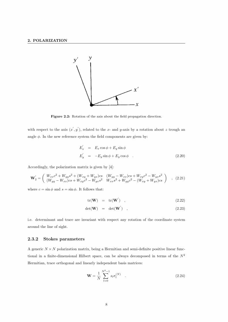
Figure 2.2: Rotation of the axis about the field propagation direction.
with respect to the axis (x′, y′), related to the x- and y-axis by a rotation about z trough an
angle φ. In the new reference system the field components are given by:
E′
x = Ex cosφ+ Ey sinφ
E′
y = −Ey sinφ+ Ey cosφ . (2.20)
Accordingly, the polarization matrix is given by [4]:
W′
2 =(Wxxc
2 +Wyys2 + (Wxy +Wyx)cs (Wyy −Wxx)cs+Wxyc
2 −Wyxs2
(Wyy −Wxx)cs+Wxyc2 −Wyxs
2 Wxxs2 +Wyyc
2 − (Wxy +Wyx)cs
), (2.21)
where c = sinφ and s = sinφ. It follows that:
tr(W) = tr(W′) , (2.22)
det(W) = det(W′) , (2.23)
i.e. determinant and trace are invariant with respect any rotation of the coordinate system
around the line of sight.
2.3.2 Stokes parameters
A generic N ×N polarization matrix, being a Hermitian and semi-definite positive linear func-
tional in a finite-dimensional Hilbert space, can be always decomposed in terms of the N2
Hermitian, trace orthogonal and linearly independent basis matrices:
W =1N
N2−1∑l=0
slσ(N)l . (2.24)
8

2.3 2D polarization
In case of a 2D planar field, N = 2, σ(2)o is the identity 2 × 2 matrix and σ
(2)l (l = 1, 2, 3) are
the Pauli spin matrices which are generators of the special unitary group SU(2) [5]:
σ(2)1 =
(1 00 −1
)σ
(2)2 =
(0 11 0
)σ
(2)3 =
(0 j−j 0
). (2.25)
The expansion coefficients sl (l = 0, 1, 2, 3) are given by:
sl = tr(Wσ(2)l ) l = 0, 1, 2, 3 . (2.26)
By using the relations (2.24,2.26) it is possible to write the elements of the polarization matrix
in terms of Stokes parameters and vice versa:
W2 =12
(so + s1 s2 + js3
s2 − js3 so − s1
), (2.27)
so = Wxx +Wyy ,
s1 = Wxx −Wyy ,
s3 = Wyx +Wxy ,
s4 = j(Wyx −Wxy) . (2.28)
The first Stokes parameter so is proportional to the intensity of the field. s1 describes the excess
in intensity of the x component with respect to the y one. s2 represents the excess of the +45
linearly polarized component over the −45 one. s3 is the excess of the right-hand circularly
polarized electric field over the left-hand one [2].
Relations (2.24-2.26) allow translating any property of the polarization matrix into a property
of the Stokes parameters. In particular, the condition (2.17) implies that the four Stokes
parameters satisfy the following inequality:
s2o ≥ s2
1 + s22 + s2
3 (2.29)
2.3.3 Unpolarized field
Let E(ω) = (Ex(ω), Ey(ω))T be a field for which:
µxy = 0 , (2.30)
independently of the particular choice of the x- and y-axis. This implies, according to (2.17-2.18)
that:
Wxy = Wyx = 0 . (2.31)
9

2. POLARIZATION
Thus, taking into account the transformation (2.21), independently of φ, i.e. independently of
the chaise of the x- and y-axis:
Wxx = Wyy . (2.32)
Hence, when (2.30) holds, considering Io = Wxx +Wyy, the polarization matrix can be written
as:
W2 =Io2
(1 00 1
). (2.33)
Thus, the polarization matrix is proportional to the unit matrix. This means that the field has
the same intensity for every direction which is orthogonal to the propagation direction of the
field. Such a field is called unpolarized or natural light, emphasizing that many natural sources
present such a behaviour [4].
2.3.4 Completely polarized field
Let E(ω) = (Ex(ω), Ey(ω))T be a field for which the x- and y-components are completely
correlated:
|µxy| = 1 . (2.34)
According to (2.18) this implies:
|Wxy| =√Wxx
√Wyy , (2.35)
considering (2.16) it follows that:
det(W2) = 0 . (2.36)
It can be shown [1; 4] that (2.34) and (2.36) are equivalent. Since the determinant is invariant
with respect to axis rotation (2.23) it follows that if (2.36) (or equivalently (2.34)) holds for a
particular pair of x- and y-directions, these equations hold for all of them. Accordingly, if the
field components are completely correlated along any pair of mutually orthogonal directions,
they are correlated for all such pairs of directions [4].
Eq (2.34), together with (2.16), implies that the polarization matrix can be written as:
W2 =(
Wxx
√Wxx
√Wyye
jα√Wxx
√Wyye
−jα Wyy
), (2.37)
where α is a real factor. A field characterized by the polarization matrix (2.37) is called
fully polarized. This terminology arises from the fact that a deterministic monochromatic
wave, which is necessarily fully polarized in the conventional sense [1], may be regarded as a
deterministic analogue of a wave of this kind [4].
10

2.3 2D polarization
Since the x- and y-components of a fully polarized field are completely correlated and its
polarization matrix is characterized by a determinant equal to zero, it follows that, conversely,
when the elements of the polarization matrix W2 factor such that W2 = E∗ET (no averaging
sign), then the determinant automatically vanishes, thus the field is fully polarized.
A fully polarized field is in general elliptically polarized, i.e. the end point of the electric field
describes a ellipse (Fig.2.3) which can reduce to a circle (circular polarization) or to a straight
line (linear polarization).
Figure 2.3: Polarization ellipse.
2.3.5 Degree of polarization
It can be shown [1; 4; 6] that the polarization matrix W2 can be uniquely decomposed into a
sum of two matrices, one corresponding to an unpolarized field and the other to a fully polarized
one [6]:
W2 = WU2 + WP
2 , (2.38)
where:
WU2 = A
(1 00 1
), WP
2 =(
B DD∗ C
), (2.39)
with A,B,C ≥ 0 and BC − DD∗ = 0. The matrix WU2 , since equal to (2.33), represents an
unpolarized field, while the matrix WP2 is of the form (2.37) and represents a fully polarized
field.
11

2. POLARIZATION
The degree of polarization, P2, can be defined as the ratio between the intensity of the polarized
part and the total intensity of the field [2; 4]:
P2 =tr(WP
2 )tr(W2)
=
√1− 4det(W2)
tr2(W2). (2.40)
After some algebra this equation can be written in a slightly different (but fully equivalent)
form [2]:
P 22 = 2
[tr(W2
2)tr2(W2)
− 12
]. (2.41)
Since trace and determinant are invariant with respect unitary transformations, P2 is indepen-
dent on the transverse reference frame. Moreover, it can be shown that [4]:
0 ≤ P2 ≤ 1 . (2.42)
When P2 = 0, it follows from (2.40) that:
(Wxx −Wyy)2 + 4WxyWyx = 0 , (2.43)
which, taking into account (2.16), can be satisfied only if:
Wxx = Wyy , (2.44)
Wxy = W ∗yx ,
which are exactly the requirements for a field to be unpolarized.
When P2 = 1 the determinant of the polarization matrix vanishes and the field is fully polarized.
Hence, when P2 equals the limiting values 0 and 1, the limiting cases of unpolarized and fully
polarized field are attained. In general, a field characterized by 0 < P2 < 1 is called partially
polarized.
It is interesting to note that (2.14) and (2.38) imply that any partially polarized electric
field can be decomposed as a superposition of an unpolarized and a fully polarized field:
E = EU + EP , (2.45)
which are mutually uncorrelated. However the two fields are not necessarily independent, since
their high-order mutual correlations may be non-zero.
The polarization matrix, being hermitian and semi-definite positive, can be decomposed as
follows [7]:
W2 = UW2
′U† = λ1u1u
†1 + λ2u2u
†2 , (2.46)
12

2.3 2D polarization
with
W′
2 = U†W2U =(λ1 00 λ2
). (2.47)
λ1 ≥ λ2 ≥ 0 are the two eigenvalues and u1, u2 are the two eigenvectors of the polarization
matrix. U is a unitary 2× 2 transformation matrix.
Since determinant and trace are invariant with respect to unitary transformations:
tr(W′
2) = tr(W2) = λ1 + λ2 , (2.48)
det(W′
2) = det(W2) = λ1λ2 .
It follows that P2 is given by:
P2 =|λ1 − λ2|λ1 + λ2
. (2.49)
From (2.48-2.49) one can readily find that:
λ1 =I
2(1 + P2), λ2 =
I
2(1− P2) , (2.50)
where I = tr(W2) is the total intensity of the field. It follows that (2.46) can be rewritten,
considering I = 1 [8]:
W2 =1 + P2
2u1u
†1 +
1− P2
2u2u
†2 , (2.51)
where † means complex conjugate transpose. Since u1u†1 and u2u
†2 are two rank-1 orthogonal
matrices it follows that W2 can be decomposed into the sum of two mutually orthogonal fully
polarized fields. However, (2.51) can be arranged as follows:
W2 = P1u1u†1 +
1− P2
2(u1u
†1 + u2u
†2) (2.52)
= P1u1u†1 +
1− P2
2I ,
where I is the identity matrix, which has two equal eigenvalues. Hence, (2.52) is of the form
(2.38), i.e. it allows decomposing W2 in the sum of an unpolarized and a fully polarized field. It
follows, conversely, that matrices with respectively two equal eigenvalues and only one non-zero
eigenvalue necessarily are of the form of (2.38).
Although (2.51) and (2.52) allow decomposing W2 in two completely different ways (wave
dichotomy) it must be pointed out that, actually, only the decomposition (2.52) is unique. In
fact, according to (2.51), an unpolarized field can be decomposed in infinite pairs of mutually
orthogonal fully polarized fields.
13

2. POLARIZATION
The degree of polarization can be also expressed in terms of the Stokes parameters. It can
be found at once from (2.27) that:
det(W) =14
(s2o − s2
1 − s22 − s2
3) , (2.53)
tr(W) = so .
It follows that:
P2 =
√s2
1 + s22 + s2
3
so. (2.54)
An unpolarized field (P2 = 0) is characterized by:
s1 + s2 + s3 = 0 , (2.55)
whereas for a fully polarized field (P2 = 1):
s2o = s2
1 + s22 + s2
3 . (2.56)
Eq. (2.56) implies that a fully polarized field can be geometrically represented as a point
(s1/so, s2/so, s3/so) on the surface of a unit radius sphere called Poincare sphere. It can be
noted that the north pole of the unit sphere corresponds to left-circular polarization, the south
pole corresponds to right-circular polarization. The points on the equator represent linearly
polarized fields. A general point on the sphere corresponds to elliptically polarized field and
antinodal points represent orthogonal states of polarization.
The unpolarized field (2.55) has its representation at the origin (0, 0, 0). A partially polarized
field (0 < P < 1) corresponds to a point within the sphere. It follows that P2 has also a direct
geometric interpretation since the set of states whose degree of polarization is P2 is the sphere
of radius P2 [5].
The degree of polarization can also be defined taking into account the correlation coefficient
µxy (2.18). Unlike P2, µxy depends on the choice of the x- and y- directions. However, one can
find an upper bound for |µxy| in terms of P2. It can be shown [1; 2] that:
P2 ≥ |µxy| . (2.57)
Hence P2 is generally greater or equal to µxy in any orthogonal (x, y) coordinate system, (2.57)
is saturated only and only if Wxx = Wyy. Thus one may find the degree of polarization of a
field by measuring the correlation coefficient (2.18) in a rotated frame in which Wxx = Wyy. It
can be shown that such a rotated frame always exists [1].
14
2.3 2D polarization
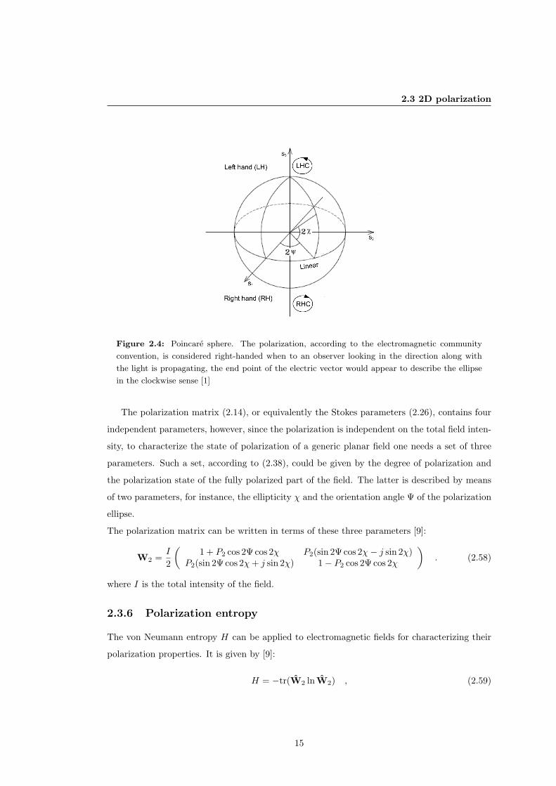
Figure 2.4: Poincare sphere. The polarization, according to the electromagnetic community
convention, is considered right-handed when to an observer looking in the direction along with
the light is propagating, the end point of the electric vector would appear to describe the ellipse
in the clockwise sense [1]
The polarization matrix (2.14), or equivalently the Stokes parameters (2.26), contains four
independent parameters, however, since the polarization is independent on the total field inten-
sity, to characterize the state of polarization of a generic planar field one needs a set of three
parameters. Such a set, according to (2.38), could be given by the degree of polarization and
the polarization state of the fully polarized part of the field. The latter is described by means
of two parameters, for instance, the ellipticity χ and the orientation angle Ψ of the polarization
ellipse.
The polarization matrix can be written in terms of these three parameters [9]:
W2 =I
2
(1 + P2 cos 2Ψ cos 2χ P2(sin 2Ψ cos 2χ− j sin 2χ)
P2(sin 2Ψ cos 2χ+ j sin 2χ) 1− P2 cos 2Ψ cos 2χ
). (2.58)
where I is the total intensity of the field.
2.3.6 Polarization entropy
The von Neumann entropy H can be applied to electromagnetic fields for characterizing their
polarization properties. It is given by [9]:
H = −tr(W2 ln W2) , (2.59)
15

2. POLARIZATION
where W2 is the density matrix [5; 9], given by:
W2 =W2
tr(W2). (2.60)
The polarimetric entropy can be regarded as a measure of the difference in the amount of
information between a fully polarized and an unpolarized state (both characterized by the
same intensity). Hence, it measures how far the field is from being completely random, i.e. in
a state which lacks all correlations between orthogonal field components [10]. Entropy can be
also expressed, in an entirely equivalent way, in terms of the eigenvalues of the density matrix:
H = −1∑k=0
λk ln λk , (2.61)
where λi = λi/tr(W2).
The entropy can be also related to the degree of polarization [9]:
H = −12
(1 + P2) ln[
12
(1 + P2)]
+12
(1− P2) ln[
12
(1− P2)]
. (2.62)
It can be noted that H is a monotonic function of P2, the maximum (H = ln 2) is achieved for
P2 = 0 and corresponds to an unpolarized field (completely random field), the minimum (H = 0)
is achieved for P = 1 and corresponds to a fully polarized field (completely deterministic field).
2.4 3D polarization
The formalism described in the previous section is applicable to fields characterized by a planar
wave front only. However, an arbitrary field fluctuates in a three dimensional space, i.e. it is
non-planar but three-dimensionally structured. This is a typical situation encountered dealing
with near fields, which are characterized by evanescent waves. Moreover, a 3D field could be
also thought of as a superposition of plane waves all travelling in different directions, without
any preferred direction, as in a cavity, for example.
A more general formalism is to be employed to describe the polarization properties of such
fields. Though the polarization matrix can readily be defined for the 3D case, it is not trivial to
define a 3D degree of polarization. In fact, unlike the 2D case, the 3D polarization matrix, in
general, cannot be decomposed into a sum of matrices describing fully polarized and unpolarized
fields. Hence, different approaches have been followed in literature to define the 3D degree of
polarization, which are generally not shared by all the optical community.
16

2.4 3D polarization
2.4.1 Polarization matrix
Let E(ω) = (Ex(ω), Ey(ω), Ez(ω))T be an arbitrary 3D field, the 3 × 3 polarization matrix is
given by1:
W3 = 〈E∗kEl〉, (k, l) = (x, y, z) , (2.63)
which can be written explicitly:
W3 =
〈E∗xEx〉 〈E∗xEy〉 〈E∗xEz〉〈E∗yEx〉 〈E∗yEy〉 〈E∗yEz〉〈E∗zEx〉 〈E∗zEy〉 〈E∗zEz〉
. (2.64)
The polarization matrix W3 has mathematically and physically analogous properties as the 2D
matrix. Since the trace is real (and gives the total spectral field intensity) and the off-diagonal
elements are complex conjugate, the matrix is Hermitian and contains nine independent real
parameters. Moreover, since det(W3) ≥ 0 it is also semidefinite positive.
As in the 2D formalism a correlation coefficient, which measures the degree of correlation
between any two of the three electric field components, can be defined [2]:
µkl = |µkl|ejβkl =Wkl√
Wkk
√Wll
(2.65)
with µlk = µ∗kl and 0 ≤ |µkl| ≤ 1.
Following a guideline similar to the 2D case, when:
|µkl| = 0, k 6= l, k, l = (x, y, z) , (2.66)
Wxx = Wyy = Wzz, thus considering I = tr(W3) = Wxx +Wyy +Wzz, the polarization matrix
can be written as:
WU3 =
I
3
1 0 00 1 00 0 1
. (2.67)
A field characterized by the polarization matrix (2.67) is called unpolarized. An upperscript U
has been added to emphasize this. It must be noted that (2.67) has three equal eigenvalues.
When the fields components are characterized by:
|µkl| = 1, ∀k, l, k, l = (x, y, z) , (2.68)
or, equivalently, when the polarization matrix can be factorized [11]:
WP3 = E∗E , (2.69)
1As the 2D case the frequency dependence is omitted and a subscript 3 is added to identify arbitrary 3D
fields
17

2. POLARIZATION
where E = (Ex, Ey, Ez) is a deterministic field, the field is fully polarized, as witnessed by the
upperscript P [11]. It must be noted that (2.69) has only one non-zero eigenvalue.
For a fully polarized 3D field the end point of the electric field vector is confined to an ellipse.
However, the plane of the polarization ellipse lies in a 3D space (Fig.2.5).
Figure 2.5: 3D polarization ellipse.
2.4.2 Stokes parameters
The 3D polarization matrix can be expanded in the form (2.24) with N = 3:
W3 =13
8∑l=0
Λlσ(3)l , (2.70)
where σ(3)o is the unitary ×3 matrix and σ3
l with l = 1 . . . 8 are the Gell-Mann matrices or the
eight generators of the SU(3) symmetry group:
σ(3)o =
1 0 00 1 00 0 1
, σ(3)1 =
0 1 01 0 00 0 0
, σ(3)2 =
0 −j 0j 0 00 0 0
,
σ(3)3 =
1 0 00 −1 00 0 0
, σ(3)4 =
0 0 10 0 01 0 0
, σ(3)5 =
0 0 −j0 0 0j 0 0
, (2.71)
σ(3)6 =
0 0 00 0 10 1 0
, σ(3)7 =
0 0 00 0 −j0 j 0
, σ(3)8 =
1√3
1 0 00 1 00 0 −2
.
18

2.4 3D polarization
The expansion coefficients are given by:
Λl =
tr(W3) l = 032 tr(W3σ
3l ) l ≥ 1 , (2.72)
and they can be regarded as 3D (spectral) Stokes parameters. They are explicitly given by [2]:
Λo = Wxx +Wyy +Wzz
Λ1 =32
(Wxy +Wyx)
Λ2 = j32
(Wxy −Wyx)
Λ3 =32
(Wxx +Wyy)
Λ4 =32
(Wxz +Wzx)
Λ5 = j32
(Wxz +Wzx)
Λ6 =32
(Wyz +Wzy)
Λ7 = j32
(Wyz +Wzy)
Λ8 =√
32
(Wxx +Wyy − 2Wzz)
(2.73)
The choice of the Gell-Mann matrices as basis leads the 3D Stokes parameters having a physical
meaning analogous to those of the 2D ones [2]. In fact, Λo is proportional to the field intensity,
Λ1 and Λ2 represent the 3D counterpart of s1 and s2 in the 2D case, as well as the pairs (Λ4,Λ5)
and (Λ6,Λ7) but referred to the xz and yz planes, respectively. Λ3 is analogous to s1 and Λ8
is related to the excess of the x- and y-spectral intensities over the z-one [2]. Following the
2D guideline an eight-dimensional Poincare sphere could be drawn which, however, would not
provide much geometrical intuition on the subject.
The polarization matrix can be written in terms of Stokes parameters:
W3 =13
Λo + Λ3 + 1√3Λ8 Λ1 − jΛ2 Λ4 − jΛ5
Λ1 + jΛ2 Λo − Λ3 + 1√3Λ8 Λ6 − jΛ7
Λ4 + jΛ5 Λ6 + jΛ7 Λo − 2√3Λ8
. (2.74)
2.4.3 Degree of polarization
The concept of the 2D degree of polarization lies in the fact that the 2D polarization matrix
can be uniquely decomposed into a fully polarized and an unpolarized part. Unlike the 2D case,
the 3D polarization matrix cannot be decomposed in its fully polarized and unpolarized part.
19

2. POLARIZATION
Hence, completely different definitions for the 3D degree of polarization, P3, can be found in
literature [5]. In the following two approaches are described which lead to physically different
degree of polarization.
According to the first approach [2; 12], the 3D degree of polarization is expressed in a form
analogous to (2.54):
P 23 =
13
∑8l=1 Λ2
l
Λ20
, (2.75)
which, by means of simple algebra, can be written in a fully equivalent form:
P 23 =
32
[tr(W2
3)tr2(W3)
− 13
]. (2.76)
It must be explicitly pointed out that, unlike the 2D case, (2.75) and equivalently (2.76) cannot
be physically read as the ratio between the polarized part and the total field intensity.
The physical consistence of the proposed degree of polarization can be recognized by considering
that, depending on traces, P 23 is independent on the orientation of the orthogonal coordinate
system. Moreover it can be shown that [2]:
0 ≤ P3 ≤ 1 . (2.77)
Since the degree of polarization is dependent on the correlations between the three orthogonal
field components and their intensities (2.76), it is useful to investigate the relationship between
P3 and µkl (2.65). In particular it can be shown that [2]:
P 23 ≥
|µxy|2WxxWyy + |µxz|2WxxWzz + |µyz|2WyyWzz
WxxWyy +WxxWzz +WyyWzz. (2.78)
The latter equation states that the square of the 3D degree of polarization is an upper bound of
the average squared correlation prevailing between the mutually orthogonal field components
weighted by the correspondent intensities [2]. This result is consistent with the intuitive physical
meaning of the degree of polarization. In the particular frame for which Wxx = Wyy = Wzz
the inequality (2.78) is saturated [2]:
P 23 =
|µxy|2 + |µxz|2 + |µyz|2
3, (2.79)
indicating that the square of the 3D degree of polarization is equal to the pure average of the
squared correlation prevailing between the three orthogonal electric field components in this
frame. It must be noted that, as well as for the 2D case, such a rotated frame always exists [2].
20

2.4 3D polarization
Since the polarization matrix is Hermitian and non negative, it can be diagonalized as (2.47)
by a suitable unitary matrix U:
W′
3 = U†W3U =
λ1 0 00 λ2 00 0 λ3
, (2.80)
where the eigenvalues λ1 ≥ λ2 ≥ λ3 ≥ 0 are real and non negative. Hence, by means of simple
algebra, (2.76) can be written as:
P3 =
√(λ1 − λ2)2 + (λ1 − λ3)2 + (λ2 − λ3)2
√2(λ1 + λ2 + λ3)
. (2.81)
It must be noted that, as well as in the 2D case (2.49), (2.81) is fully symmetric in the eigenvalues
of the polarization matrix.
It is useful to investigate what happens applying the 3D formalism for describing the polar-
ization state of a 2D field. Let E(ω) = (Ex(ω), Ey(ω)) be a generic planar field, since Ez(ω) = 0,
the polarization matrix (2.74) becomes:
W3 =13
3Λo/2 + Λ3 Λ1 − jΛ2 0Λ1 + jΛ2 3Λo/2− Λ3 0
0 0 0
.
The matrix in the upper-left corner is identical to (2.27) and is indicated as W′
2. Hence, P3,
for a field characterized by a polarization matrix W′
2, can be written as [2]:
P 23−2 = 1− 3det(W
′
2)tr2(W′
2). (2.82)
Since (2.82) is different from (2.40) the values for the degree of polarization of a 2D field
calculated in terms of the 2D and 3D formalisms are not, in general, equal [2]. Taking into
account (2.76) and (2.41) it can be shown that:
12≤ P3−2 ≤ 1 . (2.83)
This equation means that a planar field cannot be unpolarized in the 3D formalism. This result
can be explained considering that a planar field, in the 3D formalism, is restricted to oscillate
in a single plane, thus, the field must be at least partially polarized [2].
On the other hand, considering the intensity of the z component equal to zero, it can be shown
that (2.78) becomes [2]:
P 23 ≥
14
+34|µxy|2 . (2.84)
This is consistent with (2.83). In fact, for an unpolarized planar field (|µxy| = 0), P3 ≥ 1/2.
The equality holds when Wxx = Wyy. Moreover (2.84) witnesses that, for a planar field, P3 is
21

2. POLARIZATION
Figure 2.6: Differences between the 2D and 3D formalisms. Adopted from [2]
directly related to the correlation prevailing between the two nonzero electric field components
[2].
The differences between the 2D and 3D formalisms can be better appreciated by considering
Fig.(2.6) [2]. The upper row represents an unpolarized 2D field, i.e. Wxx = Wyy and |µxy| = 0,
which is passed through a polarizer. According to the 2D formalism P2 is equal to zero and
one, for the field before and after the polarizer, respectively. The bottom row represents an
unpolarized 3D field, i.e. Wxx = Wyy = Wzz and |µkl| = 0 for k 6= l, which is passed through
two devices each cutting off one of the orthogonal field components. After the first device,
which cuts off the x-component, the field becomes partially polarized (P3 = 1/2). The last
device cuts off the z-component and the field becomes fully polarized (P3 = 1). Hence, a fully
polarized 2D field is still fully polarized according to the 3D formalism, while an unpolarized
2D field, since in 3D formalism is constrained to lie in a single plane, must be at least partially
polarized.
In summary, the main difference between the 2D and 3D formalisms relies on the fact that
the latter is inherently referred to a 3D reference system, thus, the third direction is always
included albeit the corresponding intensity may be zero.
The second approach defines the 3D degree of polarization identifying the so-called “po-
larized part” of the random field [10; 13]. This procedure is based on the fact that the 3 × 3
polarization matrix can be diagonalized (2.80) and, thus, can be rewritten as:
W3 = (λ1 − λ2)UM(1)U† + (λ2 − λ3)UM(2)U† + λ3UM(3)U† , (2.85)
22

2.5 Radar polarimetry
where, M(1) and M(3) represent a fully polarized and an unpolarized 3D field, respectively,
M(2) represents an unpolarized 2D field:
M(1) =
1 0 00 0 00 0 0
, M(2) =
1 0 00 1 00 0 0
, M(3) =
1 0 00 1 00 0 1
. (2.86)
Eq. (2.85) states that a partially polarized 3D polarization matrix can be decomposed in three
matrices: 3D polarized, 2D unpolarized and 3D unpolarized. According to this approach the
degree of polarization is given by the ratio between the polarized part and the total intensity:
P =I(P )
I=
λ1 − λ2
λ1 + λ2 + λ3. (2.87)
It can be shown that 0 ≤ P ≤ 1 with P = 0 and P = 1 indicating unpolarized and fully
polarized field, respectively. It must be noted that for planar fields (λ3 = 0) P reduces to the
usual expression for the 2D degree of polarization (2.49), in fact, according to this approach the
degree of polarization is not dependent on the dimension of analysis. However, it must be noted
that, unlike the previous approach, according to (2.87) an unpolarized 2D field is unpolarized
also in 3D formalism. Moreover, it must be pointed out that (2.87) is asymmetrical in the
eigenvalues: if λ1 = λ2, then P = 0 regardless of the value of λ3.
2.5 Radar polarimetry
Up to now the description of the polarization properties of a generic partially polarized elec-
tromagnetic wave has been discussed both in the 2D and in the 3D formalisms.
The next step is to briefly describe the polarimetric interaction of waves with scattering targets.
Although this problem can be addressed both in the 2D and in the 3D formalism in this section,
since the main interest is in remote sensing applications (Chapter 5), the general polarimetric
scattering process is described as follows. A fully polarized monochromatic plane wave whose
Jones vector is given by Ei, characterized by a well-defined polarization state described accord-
ing to an orthogonal system right-hand (RH) with respect to the incident direction ı, is incident
upon a target. A receiving antenna, located at large distance from the target in a direction s,
receives the scattered plane wave Es, whose polarization state depends on the scatters’ charac-
teristics.
The scattered wave can be described either according to an orthogonal coordinate system RH
with respect to the propagation direction (Forward Scattering Alignment (FSA) convention)
or according to a RH coordinate system related to the antenna (Back-Scattering Alignment
23

2. POLARIZATION
Figure 2.7: Bistatic scattering: FSA (a); BSA (b).
(BSA) convention), see Fig.2.7. It must be noted that the BSA convention is frequently used
in backscattering configuration, since the same coordinate system is used for describing the
polarization of both the incident and the scattered waves [14; 15].
2.5.1 Scattering matrix
The scattering process, which can be regarded as a transformation of the incident wave into the
scattered one, can be described, for non-depolarizing targets, according to the Jones formalism
[1; 14; 15]:
Es = SEi , (2.88)
where Es(i) is the complex two-dimensional Jones vector of the scattered (incident) wave. S is
the 2× 2 complex scattering matrix. Equation (2.88) can be explicitly written as:(EsxEsy
)= G(r)
(Sxx SxySyx Syy
)(EixEiy
),
where (x, y) are the two wave orthogonal components defined in a plane orthogonal to the
propagation direction and G(·) is the spherical wave factor. Different definitions for G(·) can
be find in literature, however, defining it as follows [15]:
G(r) =e−jkr
kr, (2.89)
24
2.5 Radar polarimetry
the complex elements of S, called scattering amplitudes, are dimensionless [15].
It must be explicitly pointed out that, for a given frequency and scattering geometry, S depends
only on the scattering target. However, the mathematical expression of the scattering matrix of
course depends on the coordinate system adopted for describing the incident and the scattered
waves. For instance, though (2.88) is independent of the convention used (FSA or BSA),
the mathematical expression of S does depend. In particular, indicating with an overbar the
quantities referred to the BSA convention, a simple relationship between the scattering matrix
expressed in the BSA and FSA conventions, S and S, respectively, exists [14]:
S =(
1 00 −1
)S .
If the absolute phase, which cannot be measured in practice [14], is neglected, S consists of
seven independent parameters: four amplitudes and three relative phases.
Dealing with the practical case of backscattering in a reciprocal medium, the following rela-
tionships hold:
Syx = −Sxy , (2.90)
if the FSA convention is used and
Syx = Sxy , (2.91)
if the BSA convention is used. In this case the scattering matrix is sometimes called Sinclair
matrix.
It must be noted that, when (2.90) or (2.91) holds, the scattering matrix consists of five inde-
pendent parameters: three amplitudes and two relative phases.
2.5.2 Mueller matrix
The scattering matrix provides the relationship between the incident and the scattered Jones
vectors. A similar relationship between the incident and the scattered Stokes vectors (2.26) is
provided by the Mueller matrix [9; 15; 16]:
ss = (kr)−2Msi , (2.92)
where the Mueller matrix M is a real 4× 4 matrix never symmetric [15].
Although (2.92) is independent of the convention used, M, as well as S, does. As a matter of
fact, a simple relationship between M and M can be found [14; 15]:
M = U34M , (2.93)
25

2. POLARIZATION
where U34 = diag1, 1,−1,−1. This means that M can be obtained from M by changing the
signs of the third and fourth rows. This signs reversing can be explained as a change from a
RH coordinate system to a left-hand (LH) one [15].
It must be noted that for deterministic targets the scattering process can be equivalently
described by using (2.88) or (2.92), i.e. a one-to-one relationship exists between S and M [16].
For random targets, such as distributed targets (e.g. terrain, sea surface . . . ), which can be
considered composed by randomly distributed deterministic scattering centers, the two descrip-
tions are not still equivalent and (2.92) must be employed. In fact, since distributed targets
can be responsible for partially polarized scattered waves (see section 2.3.5), which cannot be
described by using the Jones vector, the Stokes formalism (2.92) in which M is replaced by the
ensemble average must be considered:
〈ss〉 = (kr)−2〈M〉si . (2.94)
It must be noted that, dealing with distributed or random targets, the one-to-one mapping
between the scattering and the average Mueller matrix is lost.
2.5.3 Kennaugh matrix
In radar application an interesting quantity is the received power given the polarization prop-
erties of the transmitting and receiving antennas. Such a power can be evaluated by using a
matrix operator called Kennaugh matrix.
Restricting the analysis to the usual monostatic configuration, indicating with sr and ss the
Stokes vectors describing the polarization properties of the radar antenna and of the scattered
field, respectively, and assuming that both a load and a polarization matching is provided, the
received power is given by [15]:
Pr =12F (λ, ϑ, ϕ)ssU4ss , (2.95)
where the function F (·) depends on the antenna gain, the electromagnetic wavelength and on
the intrinsic impedance of the free space. U4 = diag1, 1, 1,−1.
According to (2.95) the received power is simply proportional to the scalar product of sr and
ss, but with the last elements of ss reversed in sign. This result comes from the property that
polarization matching implies opposite rotation directions with respect to the antenna reference
system [14; 15]. It must be noted that this matching condition can be achieved only if both the
Stokes vectors of the antenna and of the incoming wave are referred to the antenna reference
26

2.5 Radar polarimetry
system, i.e. this is compatible with the BSA convention only [15].
By taking into account (2.92) and (2.95), the received power can be written as:
Pr =12
(kr)−2F (λ, ϑ, ϕ)sr(T )Kst , (2.96)
where (T ) stands for transpose and K is a 4 × 4 real and symmetric matrix called Kennaugh
matrix (or Stokes scattering matrix).
It can be shown that K is related to the Mueller matrix, expressed in BSA or FSA conventions,
according to the follows [14; 15]:
K = U4M = U3M , (2.97)
where U3 = diag1, 1,−1, 1. Dealing with a distributed target K must be replaced by the
ensemble average and (2.96) becomes:
Pr =12
(kr)−2F (λ, ϑ, ϕ)sr(T )〈K〉st , (2.98)
The equation (2.98) has an important theoretical and operational meaning. In detail, once
S has been measured for a given pair of polarizations (e.g. vertical and horizontal linear
polarization) the matrix K can be evaluated [14; 16] and, through (2.98), the response for any
pair of transmitted and received polarizations can be calculated. This technique is commonly
known as Polarization Synthesis [16].
It must be explicitly pointed out that, though related by a simple change of sign, M and K
correspond to completely different operators and, according to [15], must be explicitly distin-
guished by using different symbols.
The Mueller matrix, relating the incident and the scattered Stokes vectors, allows describing
the most general polarimetric scattering process.
The Kennaugh matrix allows evaluating the power received by a radar for any transmitting and
receiving polarizations.
2.5.4 Coherence matrix
In order to extend the concept of the scattering matrix to describe the behaviour of distributed
targets, the concept of the scattering vector and, accordingly, the coherence matrix are in-
troduced [17]. The main advantage of this approach is that it leads to a coherence matrix
which, since biunivocally related to the Mueller matrix, can describe the most general polari-
metric scattering mechanism. Moreover, unlike M, the coherence matrix, being Hermitian and
27

2. POLARIZATION
semidefinite positive, is decomponible in terms of elementary scattering mechanisms (Target
decomposition theorem) [17].
Following an approach similar to the one described in section 2.4.2, the scattering matrix
can be expanded in terms of the Pauli basis with expansion coefficients given by:
ki =12
tr(Sσ(2)i ) i = 0 . . . 3 . (2.99)
The complex 4× 1 vector k = [ko, k1, k2, k3]T is called scattering vector and the correspondent
coherence matrix is given by the outer product of k with its conjugate transpose (or adjoint
vector) [17]:
T = k · k† . (2.100)
For a distributed target, the coherence matrix must be defined taking into account the ensemble
average:
T = 〈k · k†〉 . (2.101)
Being Hermitian and semidefinite positive T can be diagonalized, as follows (see section 2.4.3)
[17]:
T = UΛU−1 = λ1(u1 ·u†1)+λ2(u2 ·u†2)+λ3(u3 ·u†3)+λ4(u4 ·u†4) = T1+T2+T3+T4 , (2.102)
where the matrices Ti, being related to the eigenvectors ui, are characterized by a rank equal
to one and describe deterministic scattering processes. As a matter of fact, (2.102) can be phys-
ically interpreted as the decomposition of T into four single deterministic scattering processes
whose contribute, in terms of power, is given by the appropriate eigenvalue.
One of the most important features arising directly from the eigenvalues of the coherence
matrix is the polarimetric entropy H, defined as follows [17]:
H =n∑i=1
−Pi logn Pi Pi =λi∑nl=1 λl
, (2.103)
where n = 3 for backscattering configurations and n = 4 for bistatic scattering. It must be
stressed that 0 < H < 1 is related to the degree of randomness of the scattering mechanism.
For H = 0, T is a rank one matrix with only one non-zero eigenvalue, this implies that a single
non-depolarizing scattering mechanism, characterized by a one-to-one relationship between M
and S, is in place. On the other hand, H = 1 implies that a completely random scattering
mechanism, characterized by equal and non-zero eigenvalues, which depolarizes completely the
incident wave, is in place [17]. However, most distributed natural scatters lie in between this
two extreme cases, having intermediate entropy values.
28

2.6 Conclusions
2.6 Conclusions
In this chapter the main aspects concerning wave and radar polarimetry have been discussed.
Dealing with wave polarimetry, the theory of partial polarization has been briefly described
both for the 2D case, i.e. fields characterized by a planar wave front, and for the 3D case, i.e.
fields characterized by an electric vector lying in a 3D space. The second order field correlations
and, more specifically, the polarization, have been described by using the concept of the spectral
polarization matrix which, both in 2D and in 3D, is characterized by two important properties:
it is Hermitian and semi-definite positive. Such a matrix has the same mathematical properties
of the density matrix used in quantum mechanics but different physical interpretations.
Dealing with 2D fields one needs three parameters to fully characterize the polarization
state of a partially polarized field. Since the 2D polarization matrix can be unambiguously
decomposed in terms of two matrices describing a fully polarized and an unpolarized field,
respectively, the polarization state can be determined by describing the polarization charac-
teristics of the fully polarized part and measuring the amount of polarized component in the
total field intensity (degree of polarization). It has been shown that dealing with 2D fields
several approaches can be followed to define the degree of polarization, which are completely
equivalent.
Dealing with 3D fields, the main important problem is that the 3D polarization matrix can-
not be decomposed in its fully polarized and unpolarized component, thus the well-established
2D formalism cannot be straightforwardly extended to arbitrary 3D fields. In particular, though
all the information about the polarization properties of a 3D field are contained in the 3D po-
larization matrix, a set of eight parameters for describing the polarization state of a generic 3D
field has not been identified yet. Several approaches for defining a 3D degree of polarization
have been followed in literature which lead to completely different results. In this chapter the
approaches proposed by [2] and by [11] have been discussed.
According to the first approach [2], the concept of the degree of polarization is strictly related
to the correlation prevailing between the mutually orthogonal field components. Following this
theoretical rationale a physically consistent degree of polarization, which is dependent on the
domain of observation, is defined. The latter property makes, for instance, a 2D unpolarized
field being partially polarized when described in terms of the 3D formalism. This result is not
surprising if one takes into account the inherent three-dimensional nature of the 3D degree
29

2. POLARIZATION
of polarization, which is defined with respect to three orthogonal directions, albeit the field
intensity in one of the three directions may be zero.
In the second approach [11], taking into account the Hermiticity and positive semi-definitess
properties of the 3D polarization matrix, the latter is decomposed in the eigenvalues space. In
[11] it is claimed that, following this decomposition, a fully polarized and an unpolarized compo-
nent can be straightforwardly identified to define the degree of polarization in a way analogous
to the 2D case. The proposed degree of polarization is independent of the domain of observa-
tion.
It must be pointed out that though the decomposition of the polarization matrix is straight-
forward from a mathematical viewpoint, the physical interpretation proposed in [11] is quite
unconventional, in particular, the definition of the unpolarized component does not meet the
conditions one normally expects for an unpolarized field in 3D. Accordingly, this definition
seems to be developed ad hoc to justify the proposed degree of polarization which, thus, is
quite unphysical and non-symmetric in the eigenvalues space.
In conclusions the 3D degree of polarization defined by [2] is surely more physical than the
one defined by [11] and seems to be useful for “partially” describing the polarization state of
a 3D partially polarized field. It must be pointed out that the complete description of the
polarization state of a generic 3D field is still a subject of research. From this point of view
useful insights towards further research are provided in [9].
In the last section the basic concepts of radar polarimetry have been reviewed. The po-
larimetric scattering process has been described according to both the Jones and the Mueller
formalism. Though, the two formalisms are equivalent in the case of deterministic targets,
this is not the case when dealing with distributed targets. In this latter case, the one-to-one
correspondence between the Mueller and the scattering matrix is lost and the Stokes formalism
must be employed.
The Kennaugh matrix, which allows evaluating the received power for any transmitting and
receiving antenna polarizations, has been described and its different physical meaning, with
respect to the Mueller matrix, has been remarked according to [15].
Finally the coherence matrix which, being biunivocally related to the Mueller matrix, is able to
describe the most general scattering mechanism has been introduced together with the target
decomposition theorem which allows decomposing the coherence matrix in terms of elementary
scattering mechanisms.
30
3
Rough surface scattering
3.1 Introduction
Microwave remote sensing deals with the possibility of gathering information about one or more
geophysical parameters related to the observed scene, by using active or passive sensors.
To achieve this goal the use of appropriate tailored sensors and the ability to make accurate
measurements is not enough. In fact, extract the desired information, the available measure-
ments need to be read in terms of the geophysical parameters which one is interested in, i.e. a
proper electromagnetic model is needed.
Dealing with radar applications, the basic quantity which relates the measurements to the prop-
erties of the observed scene is the normalized radar cross section (NRCS). The latter is related
to the electromagnetic field scattered by the illuminated surface. Thus, an electromagnetic
model able to describe the field scattered by a random rough surface is needed. This is the
subject of this chapter in which a general electromagnetic approach for modelling the scattering
from a random rough surface is provided.
The aim of this chapter is twofold. On one hand it sheds light on the critical aspects
which makes the problem of evaluating the field scattered from a general random rough surface
impossible to be analytically solved. Within such a framework the popular approximations are
presented to get useful analytical solutions.
On the other hand, the case of sea surface scattering, which lies at the basis of the comprehension
of the following experimental chapters, is detailed. Sea surface scattering models do not take
into account sea dynamics. These latter are particularly important when dealing with Synthetic
Aperture Radar (SAR) sea surface waves imaging, since in this case they are the geophysical
31

3. ROUGH SURFACE SCATTERING
quantities of interest. This subject is described in the last section of this chapter by discussing
a new SAR sea surface waves simulator.
3.2 Scattering coefficient
Let Eiq, Hi
q the electric and magnetic q-polarized field components of the incident plane wave,
with a harmonic time dependence exp(jωt), incident upon a surface z = ζ(x, y) from direction
ı:
Eiq = Eoe
−jkı·rq
Hiq =
1η
(ı×Eiq) , (3.1)
A p-polarized plane wave Esp, Hs
p is scattered, at large distance, into direction s.
The bistatic scattering coefficient (or bistatic NRCS), σo, is given by:
σopq(s, ı) =1Aσpq(s, ı) , (3.2)
where A is the area illuminated by the incident plane wave and σpq is the radar cross-section.
The latter is defined in such a way that, when multiplied by the incident Poynting vector
Πiq (ı) = (2η)−1|Ei
q|2 (where η the medium intrinsic impedance), one obtains the scattered
Poynting vector Πsp(s) = (2η)−1|Es
p|2 at large distance R, as if the power were uniformly
distributed in all directions:
σpq(s, ı) = 4πR2 Πp(s)Πq (ı)
. (3.3)
The area A is defined by the main lobe of the sensor antenna, but it depends also on the
incidence angle. Such dependence can be avoided by defining the scattering coefficient with
respect to the cross-section A′:
γpq(s, ı) =1A′σpq(s, ı) . (3.4)
The two scattering coefficients are simply related by:
σopq(s, ı) = γpq(s, ı) cos θi . (3.5)
In case of surface scattering both the incident and the scattered plane waves propagate in the
same medium. As a matter of fact, the ratio of the Poynting vectors in (3.3) is equal to the
ratio of the squared electric fields:
σopq(s, ı) =4πR2
A
|Esp(s)|2
|Eiq (ı)|2. (3.6)
32

3.3 General theory
A rough surface is random in nature and a statistical approach is to be followed. In partic-
ular, the surface equation is replaced by a two-dimensional random process which is assumed
to be stationary and ergodic and characterized by a zero mean :
〈ζ〉 = 0 , (3.7)
and by a standard deviation given by:
σ = 〈ζ2〉1/2 . (3.8)
Since the field scattered by a random rough surface is a random process itself, a mean scattered
field, 〈Es〉, also called coherent component, and a fluctuating scattered field or incoherent
component, Esn = Es − 〈Es〉, can be defined.
Accordingly, the scattering coefficients associated to the total field, to the coherent and the
incoherent field components, can be defined as follows:
• total scattering coefficient
σopq(s, ı) = 4πR2〈|Esp(s)|2〉A|Eiq (ı)|2
, (3.9)
• coherent scattering coefficient
σocpq(s, ı) = 4πR2|〈Esp(s)〉|2
A|Eiq (ı)|2, (3.10)
• incoherent scattering coefficient
σonpq (s, ı) = 4πR2〈|Esnp (s)|2〉A|Eiq (ı)|2
= σopq(s, ı)− σocpq(s, ı) . (3.11)
This set of relations is particularly important since they provide the link between the radar
measurements and the electromagnetic modelling of σo. This latter point is the subject of the
remaining part of the chapter. It must be pointed out that for monostatic configurations the
monostatic scattering coefficient is given, according to the BSA convention, by σopq(−ı, ı) [7].
3.3 General theory
The general problem of evaluating the field scattered by a random rough surface is a very
difficult one. In this section an attempt is made to present, in a synthetic way, a general view
of this electromagnetic problem [7].
33
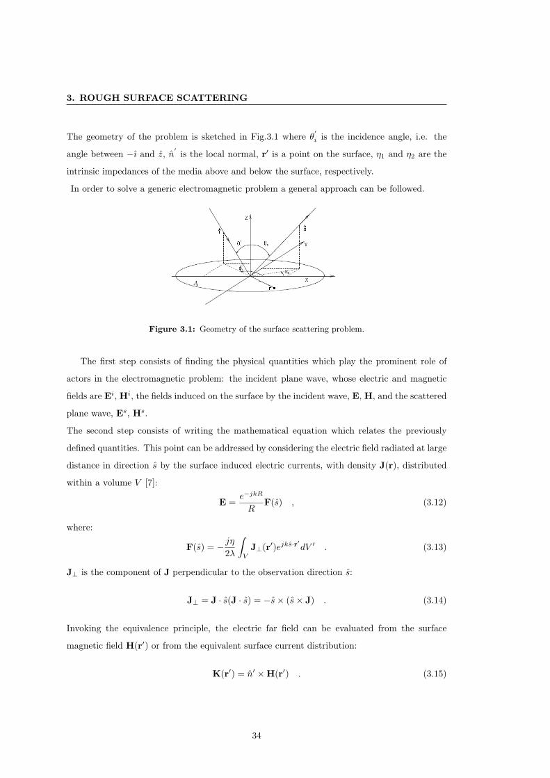
3. ROUGH SURFACE SCATTERING
The geometry of the problem is sketched in Fig.3.1 where θ′
i is the incidence angle, i.e. the
angle between −ı and z, n′
is the local normal, r′ is a point on the surface, η1 and η2 are the
intrinsic impedances of the media above and below the surface, respectively.
In order to solve a generic electromagnetic problem a general approach can be followed.
Figure 3.1: Geometry of the surface scattering problem.
The first step consists of finding the physical quantities which play the prominent role of
actors in the electromagnetic problem: the incident plane wave, whose electric and magnetic
fields are Ei, Hi, the fields induced on the surface by the incident wave, E, H, and the scattered
plane wave, Es, Hs.
The second step consists of writing the mathematical equation which relates the previously
defined quantities. This point can be addressed by considering the electric field radiated at large
distance in direction s by the surface induced electric currents, with density J(r), distributed
within a volume V [7]:
E =e−jkR
RF(s) , (3.12)
where:
F(s) = − jη2λ
∫V
J⊥(r′)ejks·r′dV ′ . (3.13)
J⊥ is the component of J perpendicular to the observation direction s:
J⊥ = J · s(J · s) = −s× (s× J) . (3.14)
Invoking the equivalence principle, the electric far field can be evaluated from the surface
magnetic field H(r′) or from the equivalent surface current distribution:
K(r′) = n′ ×H(r′) . (3.15)
34

3.3 General theory
Thus, replacing JdV ′ by KdA′ and taking into account that k = 2π/λ, the far field due to a
surface magnetic field is given by:
E(r) = jke−jkR
4πRs×
∫A′s× (n′ × ηH(r′))ejks·r
′dA′ . (3.16)
By using the duality property, a similar development can be made in case of magnetic currents
[7]. In this case the electric field at large distance due to a surface electric field E(r′) is given
by:
E(r) = −jk e−jkR
4πRs×
∫A′n′ ×E(r′)ejks·r
′dA′ . (3.17)
For a surface illuminated by a plane wave incident from direction ı with polarization defined
by the vector q (3.1), both the electric and the magnetic surface field are induced. As a matter
of fact, the electric field radiated at large distance in direction s is evaluated combining (3.16)
and (3.17):
Es(r) = −jk e−jkR
4πRs×
∫A′
[n′ ×E(r′)− s× (n′ × ηH(r′))] ejks·r′dA′ . (3.18)
The surface fields are related to the incident plane wave (3.1). Such dependence can be explicitly
taken into account by introducing the normalized surface fields eq and hq, defined as follows:
E(r′) = Eoeq(r′)e−jkı·r′
ηH(r′) = Eohq(r′)e−jkı·r′
. (3.19)
The dimensionless normalized fields depend on the form of the surface around the point r′, but
they do not depend explicitly by the displacement at that point [7].
Defining the field scattered into the direction s with polarization p:
Esp(r) = p ·Es(r) , (3.20)
equation (3.18) can be rewritten as:
Esp(r)Eo
= −jk e−jkR
4πR
∫A′Fpq(r′)ejkν·r′dA′ , (3.21)
where the vector ν is given by:
ν = k(s− ı) , (3.22)
the function Fpq(r′), which contains the surface normalized fields, is defined by:
Fpq(r′) = s [n′ × eq(r′)− s× (n′ × hq(r′))] · p , (3.23)
35
3. ROUGH SURFACE SCATTERING
and the elementary surface dA′ has the value:
dA′ =dx′dy′
n′ · z. (3.24)
Equation (3.21) can be written in a more compact, but equivalent, way:
Esp(r)Eo
= −jk e−jkR
4πRIpq , (3.25)
where the function Ipq is given by:
Ipq =∫ ∫
A
Fpq(r′)ejν·r′ dx′dy′
n′ · z. (3.26)
The area A is the horizontal projection of the illuminated surface A′.
It is important to point out that the expression (3.18) or, equivalently, (3.21) and (3.25) are
exact, since no approximation has been made to derive them.
The third step consists of evaluating the scattered field by using one of the previously devel-
oped equations. However, considering for instance (3.25), it can be noted that the evaluation
of the scattered field involves the surface fields (3.23) which are in turn to be evaluated. The
exact evaluation of the surface fields on an arbitrary random rough surface is certainly one of
the most difficult task in scattering evaluation.
3.3.1 Surface fields
Although the equations which provide the electric field radiated at large distance from the
surface as function of the surface fields are exact, the exact evaluation of the surface fields is
a very complicated task. Approximations are required both for the formulation of analytical
expressions and for numerical applications. A general approach is briefly presented in the
following [7].
The surface field, induced at a given point by a source placed at large distance, consists
of a direct contribution, from the incident field, and of an indirect contribution, from the field
scattered by the surrounding points. Accordingly, the field at a given point on the surface can
be evaluated by solving a couple of near field integral equations, as function of the field over
the whole surface. The integral equations for the medium above the surface are given by [18]:
n×E = 2n×Ei − 12πn×
∫A′jkη(n′ ×H)G− (n′ ×E)×∇′G−
(n′ ·E′)∇′GdA′
n×H = 2n×Hi − 12πn×
∫A′jk
η(n′ ×E)G− (n′ ×H)×∇′G−
(n′ ·H′)∇′GdA′ ,
(3.27)
36

3.3 General theory
where G is the Green function [7; 18]. Equations similar to (3.27) can be written for the medium
below the surface, without the terms related to the incident plane wave. The integral equations
for the medium below and above the surface, coupled by applying the boundary conditions of
continuity on the surface, can be solved by means of an iterative procedure in which the fields
inside the integrals should in turn be evaluated by similar integral equations.
Considering the Kirchhoff tangent plane field EK as first approximation, the surface electric
field is given by an equation which can be symbolically written as:
E(r) = EK(r′) +DEK(r′′) + . . . , (3.28)
where D is the integral operator. In practice, the equation (3.28) is truncated to the first order.
As a matter of fact, the surface field, according to the tangent plane approximation, depends
on the Fresnel reflection coefficients which, in turn, depend on the local incidence angle and,
therefore, on the local slopes. This means that, as far as the local slopes at any point on the
surface are known, i.e. the surface is deterministic, the surface fields can be evaluated following
this approach.
Dealing with the evaluation of the field scattered by a random rough surface, average values
are to be evaluated. This latter task can be accomplished only by making ad hoc assumptions.
In summary, the estimation of the field induced on the surface by the incident wave and the
random nature of the surface itself, make the equation (3.18) impossible to evaluate without
making simplifying assumptions. It must be pointed out that such assumptions, being valid in
a restricted range of conditions only, prevent to develop a general scattering theory and lie at
the basis of the several approaches proposed in literature [19; 20; 21].
Since the aim of this section is developing a general scattering theory, the evaluation of the
surface fields is postponed in order to derive a general expression for the bistatic scattering
coefficients. The latter are, then, specialized in the two simple limiting situations of low and
high frequency, by evaluating the correspondent surface fields.
3.3.2 Coherent scattering coefficient
Taking into account (3.25), the coherent scattering coefficient (3.10) can be written as [7]:
σocpq =k2
4πA|〈Ipq〉|2 , (3.29)
where:
〈Ipq〉 =∫ ∫
A
〈Fpq(r′)ejv·r′ 1n′ · z
〉dx′dy′ . (3.30)
37

3. ROUGH SURFACE SCATTERING
By factorizing the exponential factor as follows:
ejv·r′
= ejνzζ(x′,y′)ej(νxx
′+νyy′) , (3.31)
it can be noted that the first factor only is a random variable and need to be averaged. Moreover,
due to the stationarity, the averaged terms do not depend on the spatial coordinates and can
be singled out:
σocpq =k2
4π
∣∣∣∣〈Fpq(r′)n′ · zejνzζ〉
∣∣∣∣2 1A
∣∣∣∣∫ ∫A
ej(νxx′+νyy
′)dx′dy′∣∣∣∣2 . (3.32)
The ensemble average:
〈Fpq(r′)
n′ · zejνzζ〉 , (3.33)
involves the product of two factors. The first one does not depend explicitly on the displacement
ζ, the second one depends on the displacement. Expanding the surface in Taylor series around
a given point, one can note that the first factor depends on a set of form parameters, i.e. the
slopes, the curvatures and high order derivatives [22]. Thus, the evaluation of the average
implies that the joint probability density function (pdf) of these form parameters is available.
Moreover, if the set of form parameters, as well as the Fpq(·) function, is independent on the
displacement, the average (3.33) can be split into the product of averages:
〈Fpq(r′)
n′ · z〉〈ejνzζ〉 . (3.34)
Although this equation cannot be rigorously applied to most of the cases typically encountered,
the factorization (3.34), which is called “dishonest method”, is generally applied in all the
existing methods, since otherwise, the mathematical complexity of (3.32) would prevent any
further development. The only justification of (3.34) can be obtained a posteriori by showing
that it leads to a good approximation of the exact numerical solution [7].
The second factor in (3.34) is the characteristic function, χ(p), i.e. the Fourier transform of the
displacement pdf, evaluated for:
p = νz = k(cos θ′i − cos θs) . (3.35)
For large dimensions L ∼=√A of the illuminated area:
1A
∣∣∣∣∫ ∫A
ej(νxx′+νyy
′)dx′dy′∣∣∣∣2 = 4π2δ(νx)δ(νy) , (3.36)
38

3.3 General theory
where δ(·) is the Dirac delta function. Hence, the coherent scattering coefficient can be written
as:
σocpq =k2
4π
∣∣∣∣Fpq(r′)n′ · z
∣∣∣∣2 χ2(νz)δ(νx)δ(νy) . (3.37)
It must be noted that according to (3.37), the coherent scattering occurs essentially in the
specular directions. Moreover, to better analyze (3.37), the case of normal surface is considered.
Accordingly, χ2(·) becomes:
χ(νz) = 〈ejνzζ〉 = e−12σ
2ν2z . (3.38)
As a matter of fact, for a very rough surface (kσ 1), (3.38) vanishes. This implies that no
coherent scattering can occur for a very rough surface.
According to [19], the following property holds:∫ ∫ +∞
−∞ej(νxx+νyy)dxdy = 4π2δ(νx)δ(νy) , (3.39)
and, the coherent scattering coefficient (3.37), can be written as:
σocpq =k2
4π
∣∣∣∣Fpq(r′)n′ · z
∣∣∣∣2 χ2(νz)∫ ∫ +∞
−∞ej(νxx
′+νyy′)dx′dy′ . (3.40)
In summary, for very rough surfaces no coherent scattering occurs. For slightly rough
surfaces the coherent scattering occurs mainly into the specular direction.
3.3.3 Total scattering coefficient
Taking into account (3.25), the total scattering coefficient (3.9) can be written as:
σopq =k2
4πA〈IpqI∗pq〉 , (3.41)
where:
〈IpqI∗pq〉 =∫ ∫
A
∫ ∫A
〈Spqejv·(r1−r2)〉dx1dx2dy1dy2 , (3.42)
with
Spq = Fpq(r1)F ∗pq(r2)1
(n1 · z)(n2 · z), (3.43)
where r1 and r2 are two points on the surface, with unit normal n1 and n2, respectively. Due to
the stationarity of the random processes, the integral can be simplified by making the following
change of variables:
x = x1 − x2 y = y1 − y2
ξ =12
(x1 + x2) η =12
(y1 + y2) . (3.44)
39

3. ROUGH SURFACE SCATTERING
Performing the change of variables, the ξ and η integrals give the area A, thus (3.41) becomes:
σopq =k2
4π
∫ ∫A
〈Spqejνz(ζ1−ζ2)〉ej(νxx+νyy)dxdy . (3.45)
It must be pointed out, once again, that as far as the surface fields in Spq are known, (3.45) is
exact.
As a matter of fact, as well as for the previous case, the dishonest method is applied in order
to split the average product in (3.45):
〈Spqejνz(ζ1−ζ2)〉 = 〈Spq〉〈ejνz(ζ1−ζ2)〉 . (3.46)
The first factor is the most complicate to evaluate and approximation can be only obtained by
making appropriate assumptions which, generally, involve both the characteristic dimensions
of the surface and the electromagnetic wavelength. At this stage, in order to provide a general
approach to the scattering problem, an average function 〈Spq〉 is supposed to be available.
The second factor in (3.46) is the joint characteristic function of the displacement at two
points ζ1 and ζ2, i.e. the Fourier transform of the joint pdf of the displacement evaluated at
p = −q = νz:
χ2(p, q;x, y) = 〈ej(pζ1+qζ2)〉 . (3.47)
The dependence on the spatial separation ρ = (x, y) has been explicitly shown in (3.47). Hence,
the total scattering coefficient (3.45) becomes:
σopq =k2
4π〈Spq〉
∫ ∫ +∞
−∞χ2(νz,−νz;x, y)ej(νxx+νyy)dxdy , (3.48)
where the integration limits have been extended to infinity, assuming the dimensions of the area
A large with respect to the correlation length.
Analysing (3.48) it can be noted that the total bistatic scattering coefficient depends on the
Fourier transform of the characteristic function with respect to the spatial coordinates, evalu-
ated at Kx = νx and Ky = νy.
As a matter of fact, the main statistical surface descriptor for the evaluation of the total scat-
tering coefficient is the joint displacement pdf. In detail, a double two-dimensional Fourier
transform is needed, the first one, with respect to the displacement variables, is evaluated
for p = −q = νz, the second one, with respect to the spatial separation, is evaluated for
Kx = νx,Ky = νy. Thus, indicating with χ2(p, q;Kx,Ky) the double Fourier transform of the
joint displacement pdf, the total scattering coefficient is given by:
σopq =k2
4π〈Spq〉χ2(νz,−νz, νx, νy) . (3.49)
40

3.3 General theory
The last problem to address in order to provide an explicit formula for the total scattering
coefficient is finding a good approximation for the term 〈Spq〉. This task cannot be tackled in
a general way, since tailored approximations are to be made.
For instance, in the monostatic case and for a perfectly conducing surface, according to [20] the
following equality holds:
〈Spq〉 =4
cos2 θi, (3.50)
hence, (3.49) can be written as:
σopq =k2
π cos2 θiχ2(νz,−νz; νx, νy) . (3.51)
In summary, the basic statistical quantity required for the evaluation of the bistatic total
scattering coefficient for a random rough surface is the joint pdf of the displacement at two
points as a function of the spatial separation.
It must be pointed out that, since the joint characteristic function in (3.48) can itself be ex-
panded with respect to its statistical moments, whose Fourier transform are the spectra of
increasing order (spectrum, bi-spectrum, tri-spectrum . . . ), the scattering coefficient can be
evaluated following a different approach based on such expansion [23].
3.3.4 Incoherent scattering coefficient
According to (3.11) and taking into account (3.40) and (3.48) the incoherent scattering coeffi-
cient is given by:
σonpq =k2
4π
∫ ∫ +∞
−∞
[〈Spq〉χ2(νz,−νz;x, y)−
∣∣∣∣〈 Fpqn · z〉∣∣∣∣2 χ2(νz)
]ej(νxx+νyy)dxdy . (3.52)
3.3.5 Limiting cases
In the previous paragraphs the bistatic scattering coefficients have been derived for the total,
the coherent and the incoherent scattered field. However, it has been pointed out that the
most important problem is evaluating the source functions Fpq and Spq. This problem can be
in general tackled by solving coupled near field integral equations (3.27). In this paragraph,
approximate expressions for the surface fields and simple solutions for the scattering problem
are found in the two particular cases of a slightly rough and a very rough surface. These
approximations are also called low frequency and high frequency approximations, respectively
[7; 19].
41
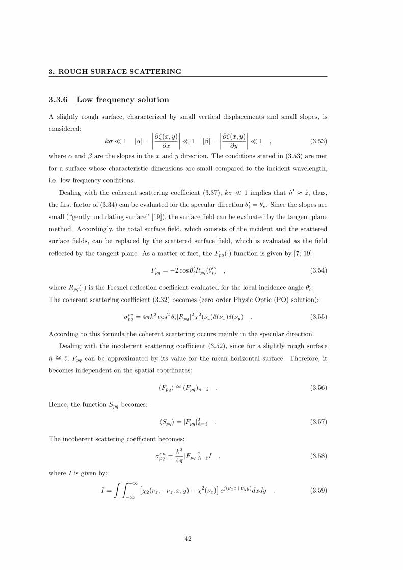
3. ROUGH SURFACE SCATTERING
3.3.6 Low frequency solution
A slightly rough surface, characterized by small vertical displacements and small slopes, is
considered:
kσ 1 |α| =∣∣∣∣∂ζ(x, y)
∂x
∣∣∣∣ 1 |β| =∣∣∣∣∂ζ(x, y)
∂y
∣∣∣∣ 1 , (3.53)
where α and β are the slopes in the x and y direction. The conditions stated in (3.53) are met
for a surface whose characteristic dimensions are small compared to the incident wavelength,
i.e. low frequency conditions.
Dealing with the coherent scattering coefficient (3.37), kσ 1 implies that n′ ≈ z, thus,
the first factor of (3.34) can be evaluated for the specular direction θ′i = θs. Since the slopes are
small (“gently undulating surface” [19]), the surface field can be evaluated by the tangent plane
method. Accordingly, the total surface field, which consists of the incident and the scattered
surface fields, can be replaced by the scattered surface field, which is evaluated as the field
reflected by the tangent plane. As a matter of fact, the Fpq(·) function is given by [7; 19]:
Fpq = −2 cos θ′iRpq(θ′i) , (3.54)
where Rpq(·) is the Fresnel reflection coefficient evaluated for the local incidence angle θ′i.
The coherent scattering coefficient (3.32) becomes (zero order Physic Optic (PO) solution):
σocpq = 4πk2 cos2 θi|Rpq|2χ2(νz)δ(νx)δ(νy) . (3.55)
According to this formula the coherent scattering occurs mainly in the specular direction.
Dealing with the incoherent scattering coefficient (3.52), since for a slightly rough surface
n ∼= z, Fpq can be approximated by its value for the mean horizontal surface. Therefore, it
becomes independent on the spatial coordinates:
〈Fpq〉 ∼= (Fpq)n=z . (3.56)
Hence, the function Spq becomes:
〈Spq〉 = |Fpq|2n=z . (3.57)
The incoherent scattering coefficient becomes:
σonpq =k2
4π|Fpq|2n=zI , (3.58)
where I is given by:
I =∫ ∫ +∞
−∞
[χ2(νz,−νz;x, y)− χ2(νz)
]ej(νxx+νyy)dxdy . (3.59)
42
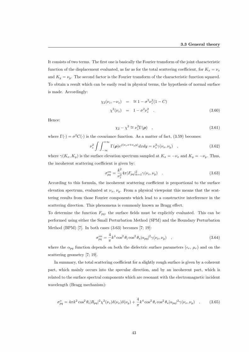
3.3 General theory
It consists of two terms. The first one is basically the Fourier transform of the joint characteristic
function of the displacement evaluated, as far as for the total scattering coefficient, for Kx = νx
and Ky = νy. The second factor is the Fourier transform of the characteristic function squared.
To obtain a result which can be easily read in physical terms, the hypothesis of normal surface
is made. Accordingly:
χ2(νz,−νz) = ∼= 1− σ2ν2z (1− C)
χ2(νz) = 1− σ2ν2z . (3.60)
Hence:
χ2 − χ2 ∼= ν2zΓ(ρ) , (3.61)
where Γ(·) = σ2C(·) is the covariance function. As a matter of fact, (3.59) becomes:
ν2z
∫ ∫ +∞
−∞Γ(ρ)ej(νxx+νyy)dxdy = ν2
zγ(νx, νy) , (3.62)
where γ(Kx,Ky) is the surface elevation spectrum sampled at Kx = −νx and Ky = −νy. Thus,
the incoherent scattering coefficient is given by:
σonpq =k2
ν2z
4π|Fpq|2n=zγ(νx, νy) . (3.63)
According to this formula, the incoherent scattering coefficient is proportional to the surface
elevation spectrum, evaluated at νx, νy. From a physical viewpoint this means that the scat-
tering results from those Fourier components which lead to a constructive interference in the
scattering direction. This phenomena is commonly known as Bragg effect.
To determine the function Fpq, the surface fields must be explicitly evaluated. This can be
performed using either the Small Perturbation Method (SPM) and the Boundary Perturbation
Method (BPM) [7]. In both cases (3.63) becomes [7; 19]:
σonpq =4πk4 cos2 θi cos2 θs|αpq|2γ(νx, νy) , (3.64)
where the αpq function depends on both the dielectric surface parameters (εr, µr) and on the
scattering geometry [7; 19].
In summary, the total scattering coefficient for a slightly rough surface is given by a coherent
part, which mainly occurs into the specular direction, and by an incoherent part, which is
related to the surface spectral components which are resonant with the electromagnetic incident
wavelength (Bragg mechanism):
σopq = 4πk2 cos2 θi|Rpq|2χ2(νz)δ(νx)δ(νy) +4πk4 cos2 θi cos2 θs|αpq|2γ(νx, νy) . (3.65)
43

3. ROUGH SURFACE SCATTERING
3.3.7 High frequency solution
A very rough surface, characterized by kσ 1 and by a large curvature radius, i.e. characterized
by characteristic dimensions large with respect to the incident wavelength (high frequency
conditions), is considered.
For kσ >> 1 the coherent part of the scattering coefficient is negligible, thus the total scattering
coefficient is equal to the incoherent one (3.52), which becomes:
σonpq =k2
4π
∫ ∫ +∞
−∞〈Spq〉χ2(νz,−νz;x, y)ej(νxx+νyy)dxdy . (3.66)
Since the correlation length is assumed to be small with respect to the dimensions L ∼=√A,
the average quantity 〈Spq〉 is a rapidly decreasing function while, for high frequency, χ2 =
〈ejνz(ζ1−ζ2)〉 is a rapidly oscillating function. As a matter of fact, the integral (3.66) can
be evaluated through an asymptotic expansion by using the stationary phase method [24].
Actually, this method can be applied directly to the integral (3.66) or to the expression of the
scattered electric field (3.21) [7; 25; 26], reported in the follows:
Esp(r)Eo
= −jk e−jkR
4πR
∫A′Fpq(r′)ejkν·r′dA′ . (3.67)
Following the latter approach, the exponential factor in (3.67) can be rewritten as:
ejν·r′
= ejΩq(x′,y′) , (3.68)
Ω = 2πL/λ increases to infinity for high frequency and q(·), given by:
q(x′, y′) =ν
k· r′
L, (3.69)
is a bounded function. The stationary points are given by:
∂ζ ′
∂x′= −νx
νz= αsp
∂ζ ′
∂y′= −νy
νz= βsp . (3.70)
It can be shown [25] that at each stationary phase point:
ν = |ν|nsp , (3.71)
which implies:
nsp =s− ı|s− ı|
. (3.72)
44

3.3 General theory
Figure 3.2: Specular point geometry.
This means that each stationary phase point is such that its local normal is bisecting the angle
between incidence and scattering directions, i.e. it is a specular reflection point [25], see Fig.3.2.
Hence, αsp and βsp in (3.70) are the slope at the specular pints.
Since the principal contribution to the integral for a given ν is given by the specular points,
the function Fpq/(n′ · z) must be evaluated at the specular points, where n′ = nsp. Therefore,
the function Spq in (3.66) has the value:
〈Spq〉 =∣∣∣∣ Fpqn · z
∣∣∣∣2sp
, (3.73)
hence, (3.66) becomes:
σonpq =k2
4π
∣∣∣∣ Fpqn · z
∣∣∣∣2sp
I , (3.74)
where the integral I is given by:∫ ∫ +∞
−∞χ2(νz,−νz; ρ)ej(νxx+νyy)dxdy . (3.75)
In case of a normal surface χ2(·) is given by (3.60). For very high frequency, χ2(·) is very small
except for small separation. Thus, the main contribute to the integral (3.75) arises around the
point x = y = 0. Thus, expanding ζ in Taylor series and limiting the expansion to the first
order terms:
νz(ζ1 − ζ2) ∼= νz(xζx + yζy) . (3.76)
This approximation is still applicable for surfaces that are not too different from a normal one.
Taking into account (3.76), the integral (3.75) becomes, after the change of variables u = νzx
45

3. ROUGH SURFACE SCATTERING
and w = νzy [7]:
I =1ν2z
∫ ∫ +∞
−∞〈ej(uζx+wζy)〉e−j(u
−νx−νz −w
−νy−νz )dudw . (3.77)
This integral, within a factor (2π)−2, is equal to the inverse Fourier transform of the slope
characteristic function, i.e. it gives the slope pdf, Tα,β(·), evaluated at the specular slopes.
Thus, the incoherent scattering coefficient becomes:
σonpq =π
(νz/k)2
∣∣∣∣ Fpqn · z
∣∣∣∣2sp
Tα,β(αsp, βsp) . (3.78)
The function Fpq can be evaluated, by taking into account the geometry around a specular point
(Fig.3.2) and by applying the high frequency hypothesis, using the tangent plane approximation,
which gives the geometric optic (GO) solution:
σonpq =π
cos4τsp|Rpq(θloc)|2Tα,β(αsp, βsp) . (3.79)
In summary, for very rough surface the total scattering coefficient is equal to the incoherent
one. This latter, depends on the Fresnel coefficient, Rpq, evaluated for the local incidence
angle, θloc, on a plane oriented in such a way that the incident and the scattering directions
describe a specular reflection and weighted for the probability, Tα,β(·), that a plane with such
an orientation exists.
It must be explicitly pointed out that such result will fail to predict the scattering coefficient
for large incidence angles for which shadowing effects can occur. Moreover, it does not take
into account multiple scattering effects.
3.4 Sea surface scattering
None of the simple methods previously described can be applied directly to the sea surface,
because many scales of roughness are superposed to give a complicate composite surface.
Although a variety of theoretical sea surface scattering models have been proposed, a good
compromise between accuracy, practical implementation and interpretation issues is achieved by
two-scale approaches [27; 28]. They are based on the assumption that the sea surface roughness
can be split into large-scale roughness (due to the long waves) and small-scale roughness (due
to the capillary and short-gravity waves), such that they satisfy the constraints posed by the
GO solution and the SPM one, respectively. These two processes are not independent since,
for instance, the non linear interaction between the capillary and gravity waves is the physical
46
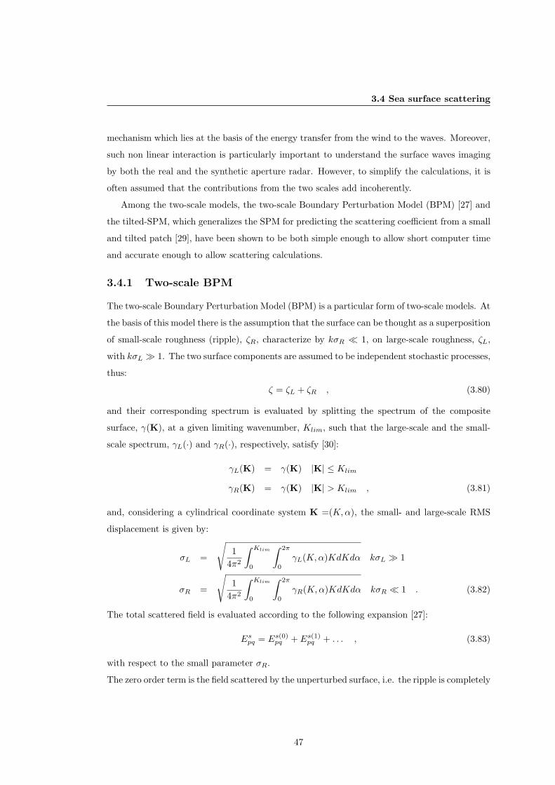
3.4 Sea surface scattering
mechanism which lies at the basis of the energy transfer from the wind to the waves. Moreover,
such non linear interaction is particularly important to understand the surface waves imaging
by both the real and the synthetic aperture radar. However, to simplify the calculations, it is
often assumed that the contributions from the two scales add incoherently.
Among the two-scale models, the two-scale Boundary Perturbation Model (BPM) [27] and
the tilted-SPM, which generalizes the SPM for predicting the scattering coefficient from a small
and tilted patch [29], have been shown to be both simple enough to allow short computer time
and accurate enough to allow scattering calculations.
3.4.1 Two-scale BPM
The two-scale Boundary Perturbation Model (BPM) is a particular form of two-scale models. At
the basis of this model there is the assumption that the surface can be thought as a superposition
of small-scale roughness (ripple), ζR, characterize by kσR 1, on large-scale roughness, ζL,
with kσL 1. The two surface components are assumed to be independent stochastic processes,
thus:
ζ = ζL + ζR , (3.80)
and their corresponding spectrum is evaluated by splitting the spectrum of the composite
surface, γ(K), at a given limiting wavenumber, Klim, such that the large-scale and the small-
scale spectrum, γL(·) and γR(·), respectively, satisfy [30]:
γL(K) = γ(K) |K| ≤ Klim
γR(K) = γ(K) |K| > Klim , (3.81)
and, considering a cylindrical coordinate system K =(K,α), the small- and large-scale RMS
displacement is given by:
σL =
√1
4π2
∫ Klim
0
∫ 2π
0
γL(K,α)KdKdα kσL 1
σR =
√1
4π2
∫ Klim
0
∫ 2π
0
γR(K,α)KdKdα kσR 1 . (3.82)
The total scattered field is evaluated according to the following expansion [27]:
Espq = Es(0)pq + Es(1)
pq + . . . , (3.83)
with respect to the small parameter σR.
The zero order term is the field scattered by the unperturbed surface, i.e. the ripple is completely
47

3. ROUGH SURFACE SCATTERING
removed. The first order term is the field due to the first order perturbations. The method is
efficient only if (3.83) can be truncated to the second term [27].
The assumption of independence between long and small roughness scales makes the bistatic
scattering coefficient given by the sum of two terms:
σopq = σopq0 + σopq1 . (3.84)
The zeroth-order term is given by the GO solution (3.79). However, the Fresnel reflection
coefficient must be replaced by an effective one, Reff,pq, which takes into account the decreasing
of the reflected power due to the ripple on the tangent plane. For large curvature radii Reff,pq
can be approximated a follows [7; 27; 30]:
Reff,pq = e−12σ
2Rν
2zRpq . (3.85)
Hence, the zeroth order scattering coefficient becomes:
σopq0 =π
cos4τsp|Reff,pq(θloc)|2Tα,β(αsp, βsp) , (3.86)
The first order scattering coefficient is evaluated averaging the small-scale result (3.64)
over the large-scale slopes [27; 31]. It is assumed that, locally, the large-scale component can be
approximated by the tangent plane. As a matter of fact, the large scale roughness is subdivided
into plane facets, which are large compared to the small-scale correlation length, but small with
respect to the large-scale curvature radius [7].
The far field scattered by the irregularities present on each facet, Es(1)pq , can be evaluated from
equivalent volume currents J(·), distributed in the space between the small ripple and the plane
facets:
Es(1)pq = − jη
2λe−jkR
R
∫Jpq(r;α, β)ejks·rdV , (3.87)
where Jpq(·) is the component along the unit vector p of the current induced by the q-polarized
incident field. α and β are the large scale slopes at the point r in which the facet is considered.
The integral is taken over the illuminated volume, which is related to the extent of the facet.
Since the small-scale process is characterized by kσR 1, the current Jpq(·) is roughly constant
along the height ζR. Moreover, the differential volume dV is given by ζRdxdy. The exponential
factor in (3.87) can be factorized as follows:
ejks·r = ejks(ζR+ζL)ejks·ρ ∼= ejksζLejks·ρ , (3.88)
48

3.4 Sea surface scattering
where the last result is obtained considering that kσR 1. Since the surface is illuminated by
a plane wave (3.1), the induced currents will be proportional to the factor e−jkı·r. The latter
can be extracted to define the following normalized function:
Hpq(r, α, β) = −j η
kEoe−jkı·rJpq(r;α, β) . (3.89)
Hence, (3.87) becomes:
Es(1)pq = k2Eo
e−jkR
4πR
∫ ∫Hpq(r;α, β)ζRejνzζLejν·ρdxdy . (3.90)
As a matter of fact, considering that the slopes are roughly constant on each facet and that,
for kσR 1, the function Hpq(r;α, β) does not vary much from point to point and can be
approximated by its average value Hpq(α, β), the total scattering coefficient (3.9) is given by:
σopq(α, β) =k4
4πA|Hpq(α, β)|2
∫ ∫ ∫ ∫〈ζR(x1, y1)ζR(x2, y2)ejνz(ζL1−ζL2)〉
ejν·(ρ1−ρ2)dx1dy1dx2dy2 .
(3.91)
By making the change of variables (3.44), the previous quadruple integral can be reduced
to a double one which, provided that the dimensions of the facet are large compared to the
small-scale correlation length, can be extended to infinity. Moreover, noting that the averaged
quantity is the small-scale covariance function Γ(x, y) and writing the large-scale displacement
in term of the facet slopes:
ζL1 − ζL2 = αx+ βy , (3.92)
equation (3.91) can be written as:
σopq(α, β) =k4
4π|Hpq(α, β)|2
∫ ∫ +∞
−∞ΓR(x, y)ej[(νx+ανz)x+(νy+βνz)y]dxdy . (3.93)
The latter integral is basically the small-scale elevation spectrum γ(Kx,Ky), evaluated at the
resonant wavenumber with components:
Kx = νx + ανz Ky = νy + βνz . (3.94)
The bistatic scattering coefficient of a single facet with given large slopes α, β can be written
as:
σopq(α, β) =k4
4π|Hpq(α, β)|2γR(νx + ανz, νy + βνz) , (3.95)
where the expression of the function Hpq, which depends on the medium properties and on the
large scale slopes, are provided in [27].
49

3. ROUGH SURFACE SCATTERING
As a matter of fact, the first order total scattering coefficient of the illuminated area is simply
the average of (3.95) over the large scale slope distribution:
σopq1 =∫ ∫
Tα,β(α, β)σopq(α, β)dαdβ . (3.96)
To read this result in more physical terms, it is convenient to rewrite (3.96) in a different,
but completely equivalent, way [27]:
σopq1 =k2
4π (νz/k)2
∫∫ ∣∣∣Hrt(K′
x,K′
y)∣∣∣2 γR(Kx,Ky)Tα,β(K
′
x,K′
y)dKxdKy , (3.97)
where
K′
x = −νx −Kx
νz, K
′
y = −νy −Ky
νz. (3.98)
The equation (3.97) represents the convolution between the small scale elevation spectrum and
the slope pdf. This means that the first order scattering coefficient can be seen as an average
over the whole wavenumber plane. As a matter of fact, the contribution of a given spectral
component is weighed by the probability that the large scale tilting makes this component to
have the right orientation and wavelength to lead the typical Bragg interference in the scattering
direction. It can be shown that if only ripples are present on the surface, Tα,β(·) reduces to a
product of Dirac delta functions and (3.97) degenerates to (3.64).
It must be explicitly stated that the first order two-scale BPM solution is exactly equal to the
tilted-SPM one [31].
One of the most important assumption to derive the first order scattering coefficient, both
according to the two-scale BPM and to the tilted-SPM approach, is that the powers scattered by
the elementary facets can be added together to evaluate the scattering coefficient. This implies
that the fields scattered by those facets are uncorrelated. The latter hypothesis is reasonable
only for facets with large dimensions compared to both the electromagnetic wavelength and
the small-scale correlation length. In other term (3.96) is valid only if the large-scale roughness
supporting the small-scale one is characterized everywhere by a large curvature radius [31].
Two-scale models are based on a decomposition of the sea surface spectrum into large and
small scales by using a limiting wavenumber Klim (3.81). The latter is to be chosen carefully in
order to meet the requirements which allows deriving the GO solution (3.86) and the first order
term (3.96), respectively [30]. In detail, the curvature radius should be much larger than the
electromagnetic wavelength everywhere, to derive the zero order term, and the surface vertical
displacements need to be small compared to the electromagnetic wavelength, to derive the first
order term. Though these constraints depend on the electromagnetic wavelength and on the sea
50

3.5 SAR sea surface waves imaging
surface roughness, which is related to a number of environmental conditions, several authors
consider a fixed value for δ = Klim/k for two-scale splitting. The range of values usually
recommended is 0.3 < δ < 0.5 [19].
In order to take explicitly into account the dependence of Klim to the environmental conditions,
Klim can be evaluated, imposing that the curvature radius is larger than the electromagnetic
wavelength and the small-scale roughness is small compared to the electromagnetic wavelength,
by solving the following expression [27; 30]:
4π2
k2
∫ Klim
0
K4S(K)dK = k2
∫ ∞Klim
S(K)dK . (3.99)
As a matter of fact, Klim is explicitly sea state dependent.
In summary, the two-scale BPM scattering model has been described. The model is ap-
plicable to those surfaces which mainly consist of a large-scale roughness, satisfying the high
frequency requirements, and a small-scale roughness, satisfying the low frequency requirements.
Since the sea surface can be thought as composed by a large-scale structure, provided by the
long waves, and by a small-scale structure, provided by the small-waves, this model works rather
well for sea surface scattering evaluation. However, it must be noted that the hypothesis of
independence between the large- and small- scale waves is not satisfied at all for the sea surface.
Generally the modulation of the small-scale roughness by the large-wave structure is taken into
account by considering a proper modulation transfer function. This point, together with the
SAR surface waves imaging, will be the subject of the next section.
3.5 SAR sea surface waves imaging
SAR imaging of a dynamic scene, such as sea surface, is considerably more complex than the
imaging of a stationary scene. In particular, though wave-like patterns are often discernible
on sea surface SAR images, obtained both from aircraft and space missions, the relationship
between such patterns and the actual sea surface wave fields is an intriguing and non-trivial
issue. From this point of view, a proper electromagnetic modelling of the scattering from a
time-variant random rough scattering surface, is very helpful both to shed light in physical
aspects governing the SAR surface waves imaging and for inversion procedures.
In this section a two-scale model, in which the sea dynamics and the interactions between
long and short waves are explicitly taken into account, is described. This model is particularly
useful to describe the SAR modulation transfer function (MTF), i.e. the function which de-
scribes the SAR sea surface waves imaging. Moreover, to better emphasize the main aspects
51
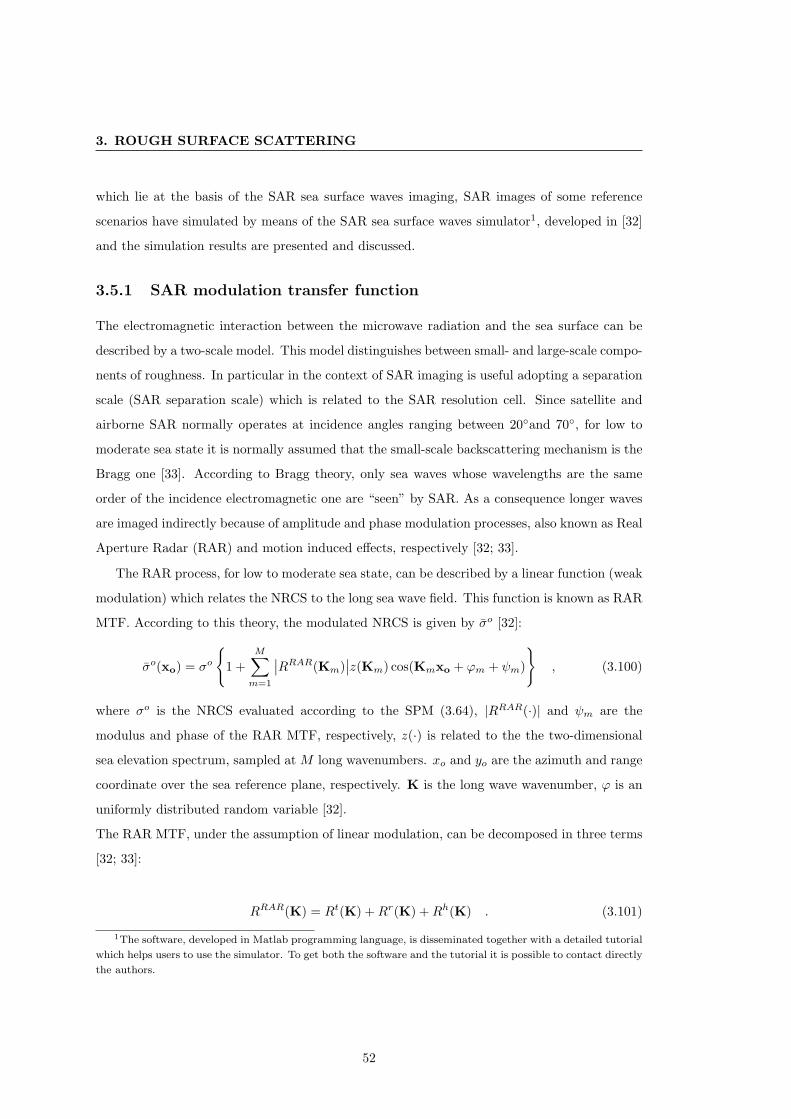
3. ROUGH SURFACE SCATTERING
which lie at the basis of the SAR sea surface waves imaging, SAR images of some reference
scenarios have simulated by means of the SAR sea surface waves simulator1, developed in [32]
and the simulation results are presented and discussed.
3.5.1 SAR modulation transfer function
The electromagnetic interaction between the microwave radiation and the sea surface can be
described by a two-scale model. This model distinguishes between small- and large-scale compo-
nents of roughness. In particular in the context of SAR imaging is useful adopting a separation
scale (SAR separation scale) which is related to the SAR resolution cell. Since satellite and
airborne SAR normally operates at incidence angles ranging between 20and 70, for low to
moderate sea state it is normally assumed that the small-scale backscattering mechanism is the
Bragg one [33]. According to Bragg theory, only sea waves whose wavelengths are the same
order of the incidence electromagnetic one are “seen” by SAR. As a consequence longer waves
are imaged indirectly because of amplitude and phase modulation processes, also known as Real
Aperture Radar (RAR) and motion induced effects, respectively [32; 33].
The RAR process, for low to moderate sea state, can be described by a linear function (weak
modulation) which relates the NRCS to the long sea wave field. This function is known as RAR
MTF. According to this theory, the modulated NRCS is given by σo [32]:
σo(xo) = σo
1 +
M∑m=1
∣∣RRAR(Km)∣∣z(Km) cos(Kmxo + ϕm + ψm)
, (3.100)
where σo is the NRCS evaluated according to the SPM (3.64), |RRAR(·)| and ψm are the
modulus and phase of the RAR MTF, respectively, z(·) is related to the the two-dimensional
sea elevation spectrum, sampled at M long wavenumbers. xo and yo are the azimuth and range
coordinate over the sea reference plane, respectively. K is the long wave wavenumber, ϕ is an
uniformly distributed random variable [32].
The RAR MTF, under the assumption of linear modulation, can be decomposed in three terms
[32; 33]:
RRAR(K) = Rt(K) +Rr(K) +Rh(K) . (3.101)
1The software, developed in Matlab programming language, is disseminated together with a detailed tutorial
which helps users to use the simulator. To get both the software and the tutorial it is possible to contact directly
the authors.
52

3.5 SAR sea surface waves imaging
The first term, Rt(·), is the tilt modulation term. It is due to a geometric tilting effect
modelling the variations of the Bragg resonant wavenumber because of the incidence angle
modulation along the long wave profile. Its contribute is stronger for HH polarization and for
range travelling waves.
The second term, Rr(·), is the range bunching modulation term. Physically, it is due to the
change of the effective backscattering area because of the slope variations along the long wave
profile. This variation of the backscattering area modulates the backscattered power per unit
area.
The third term, Rh(·), is the hydrodynamic modulation term. It is due to the interactions
between long and short waves, in particular it describes the non-uniform distribution of the
short waves over the longer ones.
The motion induced effects, are SAR inherent artifacts. They are caused by the fact that
SAR achieves a fine azimuthal resolution recording the phase history of the backscattered sig-
nals by the observed scene over a finite integration time. Thus the radial component of the
orbital motion associated with the long sea waves distort such phase history [32; 33].
In particular the radial component of the orbital velocity gives rise to the well-known velocity
bunching (VB) phenomena, i.e. scatter elements which are characterized by different orbital
velocities are non-uniformly displaced in the SAR image plane, thus apparent position of the
scattering elements are bunched and spread out [32].
The radial component of the orbital acceleration is responsible for the degradation of the az-
imuthal resolution [32]. Since both orbital acceleration and orbital velocity vary along the flight
direction they can produce a wave-like pattern onto SAR images. However for certain radar and
sea parameters the wave pattern can be severely distorted or completely smeared out [32; 33].
Actually, in addition to this acceleration induced mechanism, the azimuthal resolution is also
degraded by the sub-resolution scale variations of the orbital velocities which characterize the
different backscattering elements within the SAR resolution cell. This phenomenon can be
modelled by a scene coherence time, which is inversely proportional to the mean-square radial
velocity of the backscattering elements within a SAR resolution cell [32].
Once the main processes responsible for the wave-like formation onto SAR images have been
described, the relationship between the SAR image intensity I(x) and σo(·) can be expressed
53

3. ROUGH SURFACE SCATTERING
as follows [32]:
I(x) =∫σo(xo)ρa(xo)
δ(y − yo) exp
− π2
ρa(xo)
[x− xo −
R
Vur(xo)
]2
, (3.102)
where x = (x, y) are the azimuth and range coordinate over the SAR image plane, R and V
are slant range of the target and platform velocity, δ(·) is the Dirac delta function, ρ(·) is the
degraded azimuthal resolution and ur(·) is the radial component of the orbital velocity [32].
3.5.2 Experiments
In this paragraph some meaningful simulations, related both to single monochromatic wave and
to realistic sea wave spectrum, are shown. In all subsequent experiments reference is made to
ERS-1/2 SAR parameters [32] . The speckle noise is Weibull distributed [32].
In the first case a single 60m wavelength azimuth travelling long wave is simulated and the
noisy SAR intensity image is shown in Fig.3.3. To appreciate the results an azimuth transect
Figure 3.3: Noisy SAR (500×500) image relevant to the first experiment.
(see white dotted line in Fig.3.3) is made in the noise-free SAR image (not shown) and referred
to the corresponding long wave, see Fig.3.4, where the first 200 pixels are plotted in meters.
Since an azimuth travelling wave has been simulated, it can be noted that the SAR imaging
process is strongly non-linear in this case as clearly shown in Fig.3.4. In fact, analyzing the
plots of Fig.3.4 it is possible to recognize the non-linear effect of VB. It can be noted that, in
this case, Rt(·) is equal to zero [32; 33].
In the second case a single 100m wavelength range travelling wave is simulated and the noisy
SAR intensity image is shown in Fig.3.5. Similarly to the former case a range transect (see
54

3.5 SAR sea surface waves imaging
Figure 3.4: Plots of the 60m long ocean wave (up side) and of the simulated noise-free SAR
image transect (bottom side). Both plots are normalized to the maximum.
Figure 3.5: Noisy SAR (500×500) image relevant to the second experiment.
white dotted line in Fig.3.5) is made in the noise-free SAR image (not shown) and referred to
the corresponding long wave, see Fig.3.6. It can be noted that, in this case, the mapping is
linear. Physically, the linear imaging process is due to the fact that the VB vanishes and the
RAR MTF is maximum [33].
Finally, a more complex, i.e. realistic, sea wave field is considered. The input parameters
are shown in Table 2 and the fully-developed JONSWAP spectrum is approximated by means
of 60 wavenumbers.
In the first case a 100m peak wavelength sea spectrum made of all range travelling components
has been simulated and the relative SAR image is shown in Fig.3.7. To better understand the
SAR sea surface wave field imaging a simple one-dimensional spectral analysis can be made.
55

3. ROUGH SURFACE SCATTERING
Figure 3.6: Plots of the 100m long ocean wave (up side) and of the simulated noise-free SAR
image transect (bottom side). Both plots are normalized to the maximum.
Figure 3.7: Noisy SAR (500×500) image relevant to the third experiment.
As a matter of fact, a spectral analysis of a range transect (see dotted line in Fig.3.7), made
in the noise-free SAR image (not shown) and referred to the corresponding spectral analysis
of the sea surface displacement is shown in Fig.3.8. It can be noted that the imaging process
is essentially linear, the peak wavelength is the same both in the sea surface and in the SAR
spectrum.
In the second case a 125m peak wavelength sea spectrum, made of all azimuth travelling com-
ponents, has been simulated and the relative noisy SAR image is shown in Fig.3.9. Similarly
to the former case a spectral analysis of an azimuth transect (see white dotted line in Fig.3.9
56

3.5 SAR sea surface waves imaging
Figure 3.8: Plots of the spectral analyzed sea surface displacement (up side) and of sea-free SAR
image transect (bottom side).
Figure 3.9: Noisy SAR (500×500) image relevant to the fourth experiment.
is made in the noise-free SAR image (not shown) and referred to the corresponding sea surface
displacement spectral analysis, see Fig.3.10. The imaging mechanism is strongly non-linear. In
particular also this simple spectral analysis shows that in the SAR image spectrum the spectral
energy is shifted towards lower wavenumbers.
All this clearly shows that, when of interest, sea dynamics are a complex problem to be
incorporated in modelling. This is the case of SAR sea surface imaging [32]. Simulation results
57

3. ROUGH SURFACE SCATTERING
Figure 3.10: Plots of the spectral analyzed sea surface displacement (up side) and of sea-free
SAR image transect (bottom side).
emphasize that the SAR sea surface wave imaging is generally non linear. A linear mapping is
only possible for range and near-range travelling waves. Generally, the sea surface wave pattern
visible in SAR images is a distorted version of the real one [32]. Thus attention should be paid
in extraction the sea surface spectrum from SAR images.
3.6 Conclusions
The main aspects concerning the scattering from a random rough surface have been reviewed.
The electromagnetic background presented will be helpful to read in physical terms the next
experimental chapters.
Following a general electromagnetic approach, the scattering coefficient has been derived in a
general way, postponing the estimation of the surface fields which need restrictive hypothesis.
The scattering coefficient is found to be strictly dependent on the statistical description of the
scattering surface. Then, the scattering coefficient has been evaluated in two simple cases: very
rough surface and slightly rough surface, by properly evaluating the surface fields.
The sea surface scattering is also considered by means of the two-scale BPM, which is both
simple enough to allow short computer time and accurate enough for scattering evaluation.
Finally, the relevance of sea dynamics has been discussed by making benefit of a new SAR sea
58

3.6 Conclusions
surface waves simulator.
59

3. ROUGH SURFACE SCATTERING
60

4
Single-polarization models for sea
oil slick observation
4.1 Introduction
Sea oil pollution is a matter of great concern due to its important effects on both the economy
and on human health. Since its fine spatial resolution, day and night and practically all-weather
capabilities, the SAR is the key remote sensing tool for sea oil slick observation.
Physically, SAR oil slick observation is possible since an oil slick, damping the short gravity and
gravity-capillary waves responsible for the signal backscattered to the SAR antenna, generates
a low backscatter area, i.e. a dark area in SAR images.
However, SAR oil slick observation is not at all an easy task. In fact, due to the coherent
and narrow-band nature of the sensor, SAR images are affected by a multiplicative noise known
as speckle, which is commonly meant to hamper SAR images interpretability.
Further, other physical phenomena can also generate dark areas in SAR images. Dark areas not
related to oil spills are known as look-alike. Phenomena that give rise to look-alike include low-
wind areas, areas of wind-shadow near coasts, rain cells, currents, zones of up-welling, biogenic
films, internal waves and oceanic or atmospheric fronts [34].
Classical SAR oil slick detection can be framed into three phases: dark area detection,
features extraction, and oil slick/look-alike classification [34]. Dark area detection algorithms
are based on filtering techniques accomplished on multi-look data, i.e. SAR data in which
the speckle noise has been reduced at the expense of the spatial resolution. While dark area
detection algorithms yield the area location and the segmentation of suspected polluted areas,
61

4. SINGLE-POLARIZATION MODELS . . .
extraction of feature (e.g. geometric, radiometric and texture related) is necessary to perform
slick classification aimed at distinguishing oil slicks from look-alike. Then, the probability that
the dark area is an oil slick is evaluated.
As a matter of fact, image analysis techniques together with statistical approaches are generally
employed for SAR oil slick detection.
In this chapter, which represents the first innovative contribute to the thesis, a new paradigm
is stated: electromagnetic approaches can be usefully employed for SAR sea oil slick observa-
tion. The content of this chapter is based on paper published or submitted to international
journals and presented at international conferences [35; 36; 37; 38].
The remaining is organized as follows. In section 4.2 the speckle, which is commonly considered
as noise in SAR images and therefore to be reduced at the expense of the spatial resolution,
is firstly read in terms of the sea surface scattering mechanism and it is demonstrated to be a
source of information which can be successfully employed for SAR sea oil slick observation [35].
Following the theoretical rationale developed in section 4.2, a new SAR ship detection filter,
based on the peculiar scattering mechanism which characterizes ships, has been developed and
successfully tested in section 4.3 [36].
In section 4.4 a new electromagnetic model, based on the two-scale BPM described in sec-
tion 3.4.1, has been developed to predict the contrast, i.e. the ratio between the slick-free and
slick-covered NRCS, due to a biogenic slick [37; 38].
4.2 A new speckle model for marine full resolution SAR
images
A new physically-based speckle model for marine single-look Complex (SLC) SAR images is
here presented and investigated. The model allows using full resolution SAR images instead
of the multi-look ones in which, at the expense of a coarser spatial resolution, the speckle is
mitigated.
The proposed model is based on the generalized K (GK) pdf, which ensures a continuous
and physically consistent transition among different scattering scenarios. This speckle model
embodies Rayleigh scattering scenes, that is scenes dominated by Bragg scattering, Rice scat-
tering scenes, that is scenes with the presence of a dominant scatter, and K scattering scenes,
that is scene described by a two-scale scattering model and illuminated by an high-resolution
radar or scene in which a low backscattering area is present.
62

4.2 A new speckle model for marine full resolution SAR images
As a matter of fact, the GK parameters are read in terms of the sea surface scattering mech-
anism in order to emphasize their capabilities to detect low backscattering areas and small
dominant scatters, in marine full resolution SAR images.
The importance of this approach is twofold. From one hand it allows understanding the
effects of a low backscatter area and a small dominant scatter on the speckle distribution.
Moreover, the approach is also very interesting from an operational viewpoint dealing with oil
slick observation procedures. In fact, it allows detecting both small dark areas and ships and
this is useful since the closeness of a ship near a small dark area increases the probability that
this latter is due to an oil.
Further details can be found in [35].
4.2.1 State of art & innovative contribute
Due to the coherent and narrow-band nature of the SAR probe, SAR images are speckled.
Speckle is a multiplicative noise which makes SAR image analysis a non-trivial issue. Generally
multi-look techniques are employed in order to reduce speckle effects at the expense of the SAR
spatial resolution.
Such techniques are commonly adopted in classical SAR oil slick detection procedures in which
multi-look SAR images of 100m × 100m and gradient-like filters are employed [34; 39]. Un-
fortunately, these classical approaches hamper the possibility to detect small dark areas and
strong scatterers.
It must be explicitly noted that, since most of the oil discharged into the sea is actually due
to illegal event, e.g. oil tanker cleaning operations . . . [40], the detection of small dark areas in
SAR images is particularly important.
4.2.2 GK model
Dealing with marine scenes characterized by a Bragg scattering mechanism (3.64), a fully
developed speckle model can be assumed for the statistical fluctuations of the backscattered
signal. This is the case of sea surface when a weak large-scale modulation occurs or the area
illuminated by the radar is too large with respect to the large-scale structure [41]. In this case
the linearly polarized scattered field can be written as the sum of N elementary fields:
e(r, t) =N∑n=1
an(r, t)ejϕn(r,t) , (4.1)
63

4. SINGLE-POLARIZATION MODELS . . .
where r is the position vector, an(r, t) and ϕn(r, t) are the real form and the relative phase
factor (depending on the propagation path) governing the n-th elementary field. N , which
is the number of elementary field scattering contributions, in far-field scattering geometries is
defined by the size of the scattering region [42]. Mathematically (4.1) can be seen as a N -step
two-dimensional random walk in a complex plane where the an and ϕn represent the n-th
step length and the associated phase shift, respectively [43]. Assuming statistical independence
between the an and ϕn, if N is a given number asymptotically large, and if ϕn are
uniformly distributed, the central-limit theorem can be exploited and fully developed speckle
regime is achieved [42]. In this case the scattered field can be described by a zero-mean circular
complex Gaussian process. Hence, the field amplitude and intensity are Rayleigh and exponen-
tially distributed, respectively [42; 43].
The above mentioned assumptions of randomness and statistical independence for (4.1), al-
though likely in the case of a confused short-crested sea, may fail in presence of a large-scale
modulation due to a long-wave field [41]. Thus, under this conditions, large deviation from
Gaussian statistic is often found, particularly when an high resolution radar, such as SAR, is
considered [41]. In fact, when a SAR illuminates a sea area of linear dimensions comparable
to the longer wavelengths on the sea surface, the modulation of small-scale inhomogeneities by
the larger ones cannot be neglected and leads to the well-known bunching phenomena, which
characterizes sea surface [32]. This phenomena can be included in the random walk (4.1) taking
N as a random number fluctuating according to a negative binomial (NB) distribution, ruled
by a non-negative bunching parameter α. For N asymptotically large and under the hypothesis
of strong scattering a non-fully developed model based on the K-distribution is achieved [43].
The K pdf, relevant to the intensity of the scattered field (I ≡ |e|2), is given by [41]:
f(I) =2
Γ(α)ηα+1αα+ 1
2Iα−1
2 Kα−1
(2η
√αI
), (4.2)
where Γ(·) is the Eulerian gamma function, Kα−1(·) is the modified Bessel function of the
second kind of order α− 1 and η is the slope parameter, which corresponds to the square root
of the local mean intensity 〈I〉:
η =√〈I〉 . (4.3)
Equation (4.2) is a two-parameters function and shows a good agreement in fitting experimental
data in a wide range of non-Gaussian scattering configurations, including microwave sea echo
[35]. As α gets larger the NB distribution tends to a Poisson distribution and the shape of (4.2)
finally becomes an exponential pdf, i.e. a Rayleigh pdf for the field amplitude [43]. Hence, α is
64

4.2 A new speckle model for marine full resolution SAR images
referred as shape parameter and can be used as indicator of the departure from the Gaussian
statistics [35], a typical occurrence in marine scenes [41]. In case of low backscattering areas,
lower η and α values are expected because of their relationship with backscattered power first
and second order signal statistics, respectively [41].
In summary, the η parameter, under uniform large-scale conditions, is related to the intensity
of the local backscattering, due to the small-scale inhomogeneities and the shape parameter α
is an indicator of the departure from the Gaussian statistics [35].
According to [42; 43] it is possible to generalize this model considering a biased two-
dimensional random walk (i.e. a non-uniform phase distribution). In this case, for N large
a GK pdf is obtained. This is a three parameters pdf whose expression, for the field intensity,
is given by [43]:
f(I) =2α
Γ(α)ηα+1
(α
1 + (ν2 4α)
)α−12
Iα−1
2 Io
(ν
η
√I
)Kα−1
2η
[(1 +
ν2
4α
)αI
] 12
, (4.4)
where Io(·) is the first-kind zero-order modified Bessel function and deals with the presence of
a dominant scatterer. The ν parameter is expected to reveal the presence of a non-negligible
coherent component in the backscattered sea surface signal, due, for example, to a ship.
Unfortunately, the new physically consistent speckle model is not expected to unambiguously
distinguish between oil spills and look-alike. In fact, due to the underpinning physics at the
model basis, it is not expected a significant difference in η and α parameters values in case of
low backscattering areas relevant to oils or look-alike.
Before proceeding further it is important to note that proper estimation of the three GK pdf
parameters is an essential point to fully characterize the model [35]. Since here main concern is
on the analysis of the consistency of the physical approach, only a sub-optimal and computer
time effective parameter estimation procedure is considered. Accordingly, ν and η parameters
are estimated by means of the Rice factor, i.e. the coherent to incoherent received power ratio.
The α parameter is estimated by means of a numerical procedure, based on the χ2 test, which
minimize the L2 error norm between the measured pdf and the theoretical GK pdf, where the
α parameter is left free.
4.2.3 Experiments and discussion
The capability of the GK distribution parameters, as descriptors of marine low-backscatter
areas and dominant (although small) scatterers, is here demonstrated by means of experiments
accomplished over ERS 1/2 SLC, i.e. full resolution, SAR VV polarized C-band images. The
65

4. SINGLE-POLARIZATION MODELS . . .
SAR images were acquired by the Active Microwave Instrument (AMI) sensor mounted on
board of the ERS-1/2 satellites operated by the ESA. The nominal resolution is 10 meters in
range and 5 meters in azimuth. The proposed physical speckle characterization is compared
with the popular normalized variance approach [43] which is based on the estimation of the GK
of intensity given by:
c =〈I2〉〈I〉2
. (4.5)
It must be stressed that c is a function of both α and ν [35; 43].
The analysis is conducted evaluating the GK parameters and the c values relevant to the
different region of interest (ROIs) selected. ROIs are rectangular boxes whose size is compatible
with the χ2-test (800-900 pixels), referred to a single scattering scenario (e.g. oil, low wind,
rain cell, etc.) except for the ROIs relevant to ship and ship-wake due to the small size of these
features. Each ROI is referred to an adjacent area (not shown), which is a non-dark area without
dominant scatterers and identical in size. To further assist the parameters interpretation and
the model analysis the wind speed is evaluated by the SAR images [44]. The evaluation of the
wind speed by SAR data, although sub-optimal, allows overcoming the incorrect time/spatial
co-location between SAR data and operational wind data and retrieves the wind speed at a
finer spatial scale (1-2 Km). The retrieved wind speed is relevant to areas of linear dimensions
of about 1-2 Km, adjacent the ROIs. Wind speed is classified as low (< 3m/s), moderate (3
to 7 m/s) and high (7 to 10 m/s) [34].
The first data set is relevant to the acquisition of 26 July 1992, 9:42 UTC (ERS-1, SLCI,
orbit 5377, frame 2889, descending pass) off the coast of Malta. The SAR image regards a
sea surface area characterized by a low-to-moderate wind speed. Fig.4.1 is the quick-look of
the SLC SAR image. The ROIs, manually selected from the SLC SAR image, are shown in
Fig.4.2 which is composed by three sub-images excerpted by Fig.4.1. Visual analysis shows
that in Fig.4.2(a) several oil slicks are present; in Fig.4.2(b), near the coast of the isle of Malta,
a low wind area is present and in the top-middle of the image some ships and small oil slicks
are present. The ROIs relevant to low-wind areas are labeled as “LW”, oil slicks are labeled as
“Oil”, ships are labeled as “S” and reference sea areas are labeled as “Sea”. In Fig.4.2(c) a zoom
of the SAR image relevant to Oil4 area is shown. The same format is used in all subsequent
experiments.
In Table 4.1 the GK parameters and the normalized variance are listed for all ROIs and
corresponding reference areas. In all the cases the χ2-test of hypothesis with a 95% confidence
level was passed.
66

4.2 A new speckle model for marine full resolution SAR images
Figure 4.1: Quick-look image of the area of interest relevant to the acquisition of 26 July 1992,
9:42 UTC (ERS-1, SLCI, orbit 5377, frame 2889, descending pass) off the coast of Malta.
Figure 4.2: Zooms of three part of SAR image of Fig.4.1.
67

4. SINGLE-POLARIZATION MODELS . . .
ROI η η% α ∆α ν ν% Wind c c%
Oil 1 0.0009486 -52.9 9 -11 0.08 +14.2 Moderate 1.295 +26.22Ref. Sea 0.002014 20 0.07 1.026
Oil 2 0.0008612 -56.2 9 -22 0.02 -33.3 Moderate 1.160 +13.84Ref. Sea 0.001968 31 0.03 1.019
Oil 3 0.001568 -24.7 13 -∞ 0.02 -60 Moderate 1.144 +15.26Ref. Sea 0.002083 ∞ 0.05 0.984
Oil 4 0.001083 -48.1 4 -∞ 0.04 -20 Moderate 1.509 +44.82Ref. Sea 0.002085 ∞ 0.05 1.042
Oil 5 0.001122 -48.9 35 -∞ 0.03 -57.1 Moderate 1.101 +19.67Ref. Sea 0.002194 ∞ 0.07 0.920
Oil 6 0.0007162 -52.8 6 -34 0.03 -72.7 Low 1.270 +15.56Ref. Sea 0.001520 6 0.11 1.099
Oil 7 0.0006750 -55.6 3 -37 0.02 -81.8 Low 2.554 +132.39Ref. Sea 0.001520 40 0.11 1.099
LW 1 0.0002059 -81.2 41 -13 0.04 -42.8 Low 1.085 +4.73Ref. Sea 0.001093 54 0.07 1.036
LW 2 0.0009361 -29.7 1 -∞ 0.04 0.0 Low 1.819 +95.59Ref. Sea 0.001331 ∞ 0.04 0.930
S1 0.01387 +950 NA − 0.26 +766 Low 4.213 +317.13Ref. Sea 0.001320 ∞ 0.03 1.010
S2 0.01225 +828 NA − 0.45 +1400 Low 1.999 +78.32Ref. Sea 0.001320 ∞ 0.03 1.121
Table 4.1: Measured GK parameters and c values relevant to ROIs of Figs.4.2(a-b).
68

4.2 A new speckle model for marine full resolution SAR images
The analysis of the three GK parameters shows that η values in all the low backscattering
areas are always lower that the corresponding reference areas. Higher η values are experienced
for areas with a dominant scatterer. Results are in agreement with the theoretical expectations
of the previous section.
Dealing with α, it must be noted that the notation “∞” is used to emphasize that an
high value (> 60) is measured, it means that a Gaussian scattering regime is in place. α values
relevant to low backscattering areas are always lower than the reference ones describing a strong
departure from the Gaussian scattering regime. This is in total accordance to what stated in
[41]. A closer look to the case of Oil5 shows that now a lower α value is achieved respect to
other oil covered areas (see Table 4.1). This can be physically justified by a weaker oil damping
which may be related to oil age, oil type and to weathering effects [45]. Concerning S1 and S2,
the estimation procedure fails to estimate the α value because the measured pdf (not shown
to save space) shows some gaps and bins with very few number of samples [46]. The notation
“NA” is used to emphasize this.
Dealing with ν, it is not useful to detect low backscattering areas, since it is physically
related to the presence of a coherent component in the backscattered field. As expected, in S1
and S2, ν values are greater than usual ones. It must be noted however that surprisingly ν
is not as large as one would expect and, in order to explain such unexpected result a detailed
analysis was accomplished. Relevant pdfs (not shown) are indistinguishable from a K pdf, but
for some strong isolated outliers witnessing the presence of few strong dominating scatterers.
As matter of fact, a Rice pdf is not achieved. The comparison with the measured c values shows
that it is not possible to clearly distinguish between low backscattering areas and areas with
a dominant scatterer. This result can be justified both considering that c = c(α, ν) does not
sort the two physical information due to α and ν, and by the analysis of the theoretical c curve
shown in [43]. To better appreciate the results differential parameters η%, ∆α, ν% and c% have
been introduced. They are defined as follows:
x% =(xROI − xRef
xRef
)· 100 , (4.6)
where x can be η, ν or c; and
∆α = αROI − αRef . (4.7)
Dealing with η% all these experiments show that low backscattering areas are characterized
by a negative value around 50%. This is untrue for the Oil3 and LW2 ROIs, where η% value
is negative but higher. This can be physically explained by the sea-oil mixing occurring in the
69

4. SINGLE-POLARIZATION MODELS . . .
Oil3 area and in general by the heterogeneity of these two ROIs, see Fig.4.2. It is also important
to note that the S1 and S2 ROIs, characterized by the presence of a ship, exhibit a very high
positive η% value.
An high negative ∆α value, witnessing a change of the scattering regime, characterize the low
backscattering areas. In particular, when the scattering regime changes from the non-Gaussian
to the Gaussian case ∆α is equal to −∞, when scattering regime changes from different non-
Gaussian cases ∆α is finite and negative.
ν% values emphasize the presence of a non negligible coherent component. The c% values
confirm the limit of the normalized variance.
In view of an operational use of the approach, its sensitivity with respect to the choice
of the reference area has been made [35]. Results show that there is a limited variability for
both η and α when Sea ROIs are considered, while the Oil8 ROI is well detected even if the
reference area is changed. Dealing with ν, high values variability is experienced for Sea ROIs.
Although there is no clear and unique physical explanation, it does not affect the capability
to distinguish low backscattering areas, since not used, and ships, since the variability is well
below the dominant scatterer levels.
The second data set is related to the acquisition of 16 July 1992, 9:56 UTC (ERS-1, SLCI,
orbit 5234, frame 2871, descending pass) off the Tunisian coast. The SAR image regards a sea
surface area characterized by a moderate wind speed. Fig.4.3 shows the quick-look of the SAR
image and the selected ROIs are relevant to oil slicks, a low wind area, a ship with its wake
(labeled as SW) and a dark area due to a current (labeled as “C”). All results, which are in
total agreement to what formerly experienced, are shown in Table 4.2. The only cases that
need a further comment are relevant to the C and SW ROIs. These latter results show that
it is not possible to distinguish such features from the other low backscattering areas since the
GK parameters values are similar to other ones. However, it must be noted that ship wakes
may be difficult to be detected since it is generally expected that in the ROI only few values,
not heterogeneous enough with respect to the surrounding sea, refer to the wake and therefore
the estimated GK parameters may be not appreciably changed.
The third data set is related to the acquisition of 02 June 2003, 21:02 UTC (ERS-2, SLCI,
orbit 42439, frame 1107, ascending pass) relevant to a well-known oil spill accident widely
studied and documented [35]. Fig.4.4 shows the quick-look of the SAR image and the selected
ROIs which are all relevant to oil slicks. The oil slick of about 39 kmq offshore south of the
Swedish coast caused by the Fu Shan Hai bulk carrier accident which occurred north of the
70
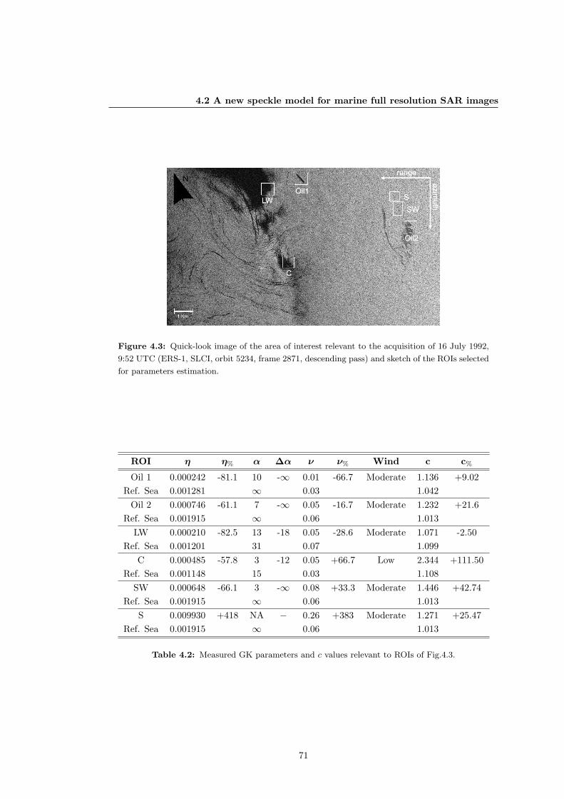
4.2 A new speckle model for marine full resolution SAR images
Figure 4.3: Quick-look image of the area of interest relevant to the acquisition of 16 July 1992,
9:52 UTC (ERS-1, SLCI, orbit 5234, frame 2871, descending pass) and sketch of the ROIs selected
for parameters estimation.
ROI η η% α ∆α ν ν% Wind c c%
Oil 1 0.000242 -81.1 10 -∞ 0.01 -66.7 Moderate 1.136 +9.02Ref. Sea 0.001281 ∞ 0.03 1.042
Oil 2 0.000746 -61.1 7 -∞ 0.05 -16.7 Moderate 1.232 +21.6Ref. Sea 0.001915 ∞ 0.06 1.013
LW 0.000210 -82.5 13 -18 0.05 -28.6 Moderate 1.071 -2.50Ref. Sea 0.001201 31 0.07 1.099
C 0.000485 -57.8 3 -12 0.05 +66.7 Low 2.344 +111.50Ref. Sea 0.001148 15 0.03 1.108
SW 0.000648 -66.1 3 -∞ 0.08 +33.3 Moderate 1.446 +42.74Ref. Sea 0.001915 ∞ 0.06 1.013
S 0.009930 +418 NA − 0.26 +383 Moderate 1.271 +25.47Ref. Sea 0.001915 ∞ 0.06 1.013
Table 4.2: Measured GK parameters and c values relevant to ROIs of Fig.4.3.
71
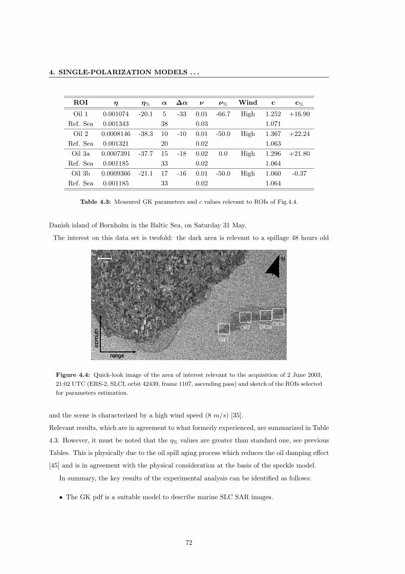
4. SINGLE-POLARIZATION MODELS . . .
ROI η η% α ∆α ν ν% Wind c c%
Oil 1 0.001074 -20.1 5 -33 0.01 -66.7 High 1.252 +16.90Ref. Sea 0.001343 38 0.03 1.071
Oil 2 0.0008146 -38.3 10 -10 0.01 -50.0 High 1.367 +22.24Ref. Sea 0.001321 20 0.02 1.063Oil 3a 0.0007391 -37.7 15 -18 0.02 0.0 High 1.296 +21.80
Ref. Sea 0.001185 33 0.02 1.064Oil 3b 0.0009366 -21.1 17 -16 0.01 -50.0 High 1.060 -0.37
Ref. Sea 0.001185 33 0.02 1.064
Table 4.3: Measured GK parameters and c values relevant to ROIs of Fig.4.4.
Danish island of Bornholm in the Baltic Sea, on Saturday 31 May.
The interest on this data set is twofold: the dark area is relevant to a spillage 48 hours old
Figure 4.4: Quick-look image of the area of interest relevant to the acquisition of 2 June 2003,
21:02 UTC (ERS-2, SLCI, orbit 42439, frame 1107, ascending pass) and sketch of the ROIs selected
for parameters estimation.
and the scene is characterized by a high wind speed (8 m/s) [35].
Relevant results, which are in agreement to what formerly experienced, are summarized in Table
4.3. However, it must be noted that the η% values are greater than standard one, see previous
Tables. This is physically due to the oil spill aging process which reduces the oil damping effect
[45] and is in agreement with the physical consideration at the basis of the speckle model.
In summary, the key results of the experimental analysis can be identified as follows:
• The GK pdf is a suitable model to describe marine SLC SAR images.
72

4.3 A physically based SAR ship detection filter
• The three GK parameters are suitable descriptors of dark areas and areas with a dominant
scatterer.
• The c parameter is not suitable for distinguishing among dark areas and areas with a
dominant scatterer.
• Dark areas are characterized by low and negative η% values and negative ∆α values.
• This approach, as far as the one based on the normalized variance, is not able to discrim-
inate among the physical causes generating dark areas.
• Dark areas due to oil slicks are characterized by η% value related to the aging process.
• Areas with a small dominant scatterer are characterized by a positive and very high η%
value, an α value which can not be estimated and a very high and positive ν% value.
In conclusion it is possible to state that the GK speckle model, since able to embody very
different marine scattering cases, allows taking advantage of full-resolution SAR images and
detecting even small dark areas and dominant scatterers. The experimental results demonstrate
the physically consistence of the model.
Dealing with SAR sea oil slick detection, the approach can be envisaged as an additional tool
to assist classical detection procedures. In fact, classical oil spill detection approaches are not
able to process such speckled SAR images and, therefore, deal with multi-look SAR images
where, at the expense of a poorer spatial resolution, the speckle is mitigated. Unfortunately,
this classical approach hampers the possibility to detect small dark areas and strong scatterers
which are very difficult to be identified by means of usual filtering techniques.
Unlike the classical procedures, the new proposed approach is able to detect simultaneously
small dark areas and small dominant scatterers (typically ships). This is very important because
it is highly probable that a dark area near a ship is due to an illegal discharge.
4.3 A physically based SAR ship detection filter
SAR ship detection is an important application in the context of environment and security
monitoring. It allows monitoring traffic, fisheries, and associating ships with oil discharge over
wide areas with high spatial resolution almost independently from weather conditions and both
day and night time.
Since full-resolution SAR images are heavily affected by the presence of speckle, ship detection
73

4. SINGLE-POLARIZATION MODELS . . .
algorithms generally employ speckle reduced SAR images at the expense of a degradation of
the spatial resolution.
A new physical approach is here proposed, which considers ships as dominant scatterers and
therefore responsible for a strong and coherent backscattered signal. Based on this rationale, a
new simple and very effective filtering technique, which is able to process full-resolution SAR
images, has been conceived and implemented. The filtering technique is both computationally
effective and able to detect with a good accuracy and low false alarm rate the ships.
Further details can be found in [36]
4.3.1 State of art & innovative contribute
Physically, backscatter from ships is determined by several scattering mechanisms including
direct reflection from areas perpendicular to the radar beam, corner reflections and multiple
reflections from the ship and sea surface which cause a bright spot over SAR images. Other
factors which come into play are: construction material and characteristics of the radar instru-
ment, such as incidence angle, frequency, polarization, resolution and speckle [47].
However, there are several processes and objects which may generate false alarms in SAR ship
detection procedures. False alarms are most prevalent in non-homogeneous areas of the imagery,
such as changes in ocean backscatter caused by variations in surface wind speed and direction
or the transition regions between different wind conditions. Moreover, many other processes
may generate false alarms: oceanographic phenomena (e.g. atmospheric fronts, internal waves,
current boundaries or breaking waves), outlying rocks, shoals, sea currents and coastal effects
[48].
Usually, ship detection systems are framed into four fundamental stages: land masking,
pre-processing, pre-screening, and discrimination [48]. Most ship detection systems include
a preliminary stage in which land areas are masked out of the image being processed. Pre-
processing is aimed at making the subsequent detection stages easier; a typical practice consists
in the speckle filtering which increases the contrast achieved but at the expense of a degradation
of the resolution. Algorithms searching within the whole image for potential ship pixels are
referred to as pre-screening algorithms. Finally, at last stage, which is referred to as the discrim-
ination one, the false alarms are identified and removed. Generally, pre-screening algorithms
locate potential ship signatures by finding local regions that are statistically different from the
background, via either comparison of local statistics or considering threshold values [48]. Since
the background backscatter changes substantially with SAR incidence angle, wind speed, and
74
4.3 A physically based SAR ship detection filter
sea state, various algorithms have been developed which automatically adapt to changing back-
ground backscatter during the search for targets. Many of these algorithms are referred to as
Constant False-Alarm Rate (CFAR) algorithms. An important issue in using these algorithms
is the choice of the threshold value (t) which is related to a prescribed false-alarm rate. Other
approaches use cross-correlation of sub-apertures or explore a wavelet-based technique [36].
A different approach is here proposed for single polarization SAR data.
From an electromagnetic point of view, a ship can be considered as a dominant scatterer
characterized by a strong and coherent backscattered signal. This important feature can be
taken into account by evaluating the sub-resolution electromagnetic field formation, i.e. the
speckle. Within such a framework the key parameter is the Rice Factor (RF) which is expected
to be sensitive to the presence of a dominant scatterer such as a ship [35].
Based on this rationale a new simple and very effective filtering technique, which is able to
process full-resolution SAR images is developed.
4.3.2 Ship detection
In general, ships, in single polarization SAR imagery, appear as individual pixels or groups
of pixels which are bright compared to their surroundings. From an electromagnetic point of
view, a ship can be considered as a dominant scatterer, characterized by a strong coherent
component of its backscattered signal. This behavior is theoretically and practically confirmed
by the physically based Generalized-K distribution model for full-resolution, i.e. speckled, SAR
images presented in [35].
Supported by this theoretical background, a new filtering technique to detect ships over
high resolution SAR images is proposed. The proposed filter concerns the pre-processing, pre-
screening and discrimination stages of the ship detection chain and can be described according
to the following rationale: the presence of a non-negligible coherent component in the backscat-
tered sea surface signal can be highlighted by evaluating the corresponding Rice Factor image of
the area under study [35]. The RF represents the coherent-to-incoherent received power ratio of
the backscattered signal [49]. Hence, the pre-processing stage consists in evaluating the RF of
the calibrated SAR image. In order to expedite time processing, the SAR image is partitioned
into 100 × 100 pixels wide tiles and, within each tile, a moving local window is applied. The
local window evaluates the coherent power over a 3×3 pixels region while the incoherent power
is evaluated over the entire tile (see Fig.4.5).
75

4. SINGLE-POLARIZATION MODELS . . .
These are then compared to determine the RF as:
RF =[mean(σolocalwindow)]2
2 [std(σotile)]2 . (4.8)
Figure 4.5: Sketch of the filtering procedure.
The dimension of the local window is set to minimize the unavoidable decrease of the native
image resolution and to allow a better detection of the small ships, and the dimension of the
tiles is set to get a stable reference background level.
The successive step, i.e. the pre-screening stage, involves a method of searching for “bright
anomalies” in the RF image. It consists in an adaptive threshold algorithm designed to search
for pixel values which are unusually high compared to those in the surrounding area. Pixel
values which lie above the threshold are considered high and therefore likely to correspond to a
dominant scatterer. Since it can be proved that the RF image follows a log-normal distribution,
a threshold which gives a constant false-alarm probability is set. Hence, t is evaluated, for each
tile, according to the relationship:
t = elnµRF+TσRF , (4.9)
where µRF and σRF are the tile’s mean and standard deviation, respectively, and T is the
parameter which determines the false alarm probability, PFA, which in the propose approach
has been empirically set 10−3 [50].
The pre-screening stage output consists in all the pixels that are characterized by a RF
which is higher with respect to local background. It was experienced that these pixels are
relevant to the ships as well as a specific type of false-alarm due to the transition between areas
characterized by a low NRCS values, e.g. low-wind areas, and areas characterized by higher
NRCS values but still relevant to sea surface. This feature is taken into account to perform
the discrimination stage in an unsupervised configuration, i.e. to remove the false-alarms. In
76
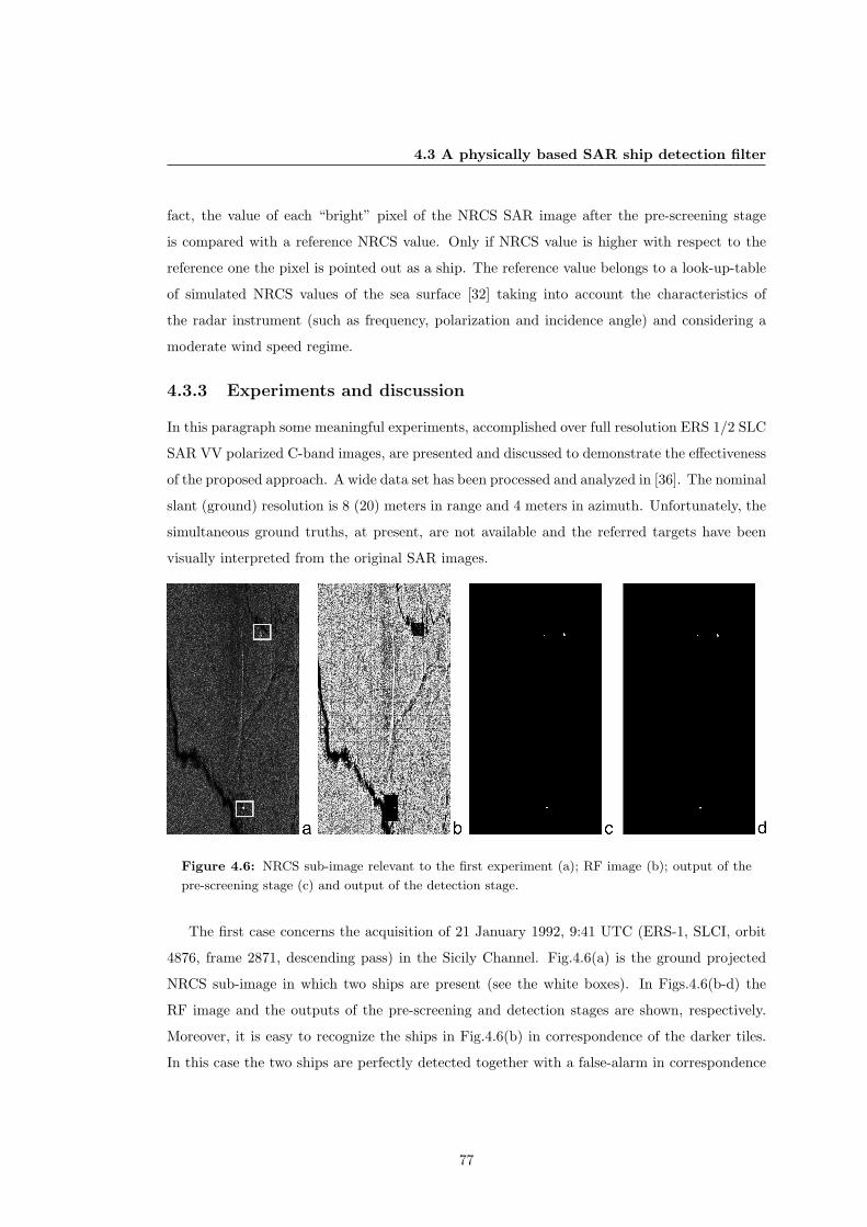
4.3 A physically based SAR ship detection filter
fact, the value of each “bright” pixel of the NRCS SAR image after the pre-screening stage
is compared with a reference NRCS value. Only if NRCS value is higher with respect to the
reference one the pixel is pointed out as a ship. The reference value belongs to a look-up-table
of simulated NRCS values of the sea surface [32] taking into account the characteristics of
the radar instrument (such as frequency, polarization and incidence angle) and considering a
moderate wind speed regime.
4.3.3 Experiments and discussion
In this paragraph some meaningful experiments, accomplished over full resolution ERS 1/2 SLC
SAR VV polarized C-band images, are presented and discussed to demonstrate the effectiveness
of the proposed approach. A wide data set has been processed and analyzed in [36]. The nominal
slant (ground) resolution is 8 (20) meters in range and 4 meters in azimuth. Unfortunately, the
simultaneous ground truths, at present, are not available and the referred targets have been
visually interpreted from the original SAR images.
Figure 4.6: NRCS sub-image relevant to the first experiment (a); RF image (b); output of the
pre-screening stage (c) and output of the detection stage.
The first case concerns the acquisition of 21 January 1992, 9:41 UTC (ERS-1, SLCI, orbit
4876, frame 2871, descending pass) in the Sicily Channel. Fig.4.6(a) is the ground projected
NRCS sub-image in which two ships are present (see the white boxes). In Figs.4.6(b-d) the
RF image and the outputs of the pre-screening and detection stages are shown, respectively.
Moreover, it is easy to recognize the ships in Fig.4.6(b) in correspondence of the darker tiles.
In this case the two ships are perfectly detected together with a false-alarm in correspondence
77

4. SINGLE-POLARIZATION MODELS . . .
of the arched feature in the middle of the image (see Fig.4.6(a)). No differences are experienced
between the pre-screening and the detection stages outputs.
Figure 4.7: NRCS sub-image relevant to the second experiment (a); RF image (b); output of
the detection stage.
The second case concerns the acquisition of 26 July 1992, 9:42 UTC (ERS-1, SLCI, orbit
5377, frame 2871, descending pass) off the Portuguese Sicilian coasts. The NRCS sub-image
is shown in Fig.4.7(a) and concerns a sea area in which there are bright patterns due to the
internal waves and two ships, highlighted by the white boxes. This case is interesting for the
presence of the bright internal waves which are typical features that generate false alarms.
In Figs.4.7(b-c) the RF image and the output of detection stage are shown, respectively. In
this the case, the two ships are perfectly detected and, very important aspect, no false-alarms
are detected. No differences are experienced between the pre-screening (not shown) and the
detection stages outputs.
In conclusion, a new filtering procedure to detect ships over full-resolution SAR images has
been proposed. It is physically based on the use of the Rice Factor parameter to highlight
the presence of a dominant scattered. A set of meaningful experimental results, concerning
very challenging cases such as presence of rain cells or internal waves, is shown [36]. The
filtering procedure has shown to be both computationally effective and able to operate over
fully-speckled SAR images. Moreover, the proposed technique is able to detect ships with good
accuracy and with low false alarms [36].
4.4 A two-scale BPM contrast model
In this section the sea surface scattering is analyzed, in the frame of the two-scale BPM, to
develop a new physically based model for predicting the contrast, i.e. the ratio between the
slick-free and slick-covered NRCS, due to a biogenic slick.
78

4.4 A two-scale BPM contrast model
Biogenic surface slicks, produced for instance by plankton and animals in the ocean and gen-
erally visible on the water surface only at low to moderate wind conditions, represent one of
the most intriguing problem in radar oil slick observation, since they visually resemble like oil
slicks in radar images [51]. As a matter of fact, a physically based and computer-time effective
contrast model is particularly important both for a better understanding of the biogenic slicks’
effects on the sea surface scattering mechanism and, therefore, to improve radar based oil slick
observation techniques. Dealing with the latter aspect, such a modelling can be very helpful
both for evaluating a physically based threshold in dark area detection algorithms (instead of
the commonly used empirical thresholds [34; 52; 53]) and for developing the theoretical back-
ground which can allow distinguishing oil slicks from look-alike. Further details can be found
in [37; 38].
4.4.1 State of art & innovative contribute
In literature, only few studies have been addressed for developing a physically consistent contrast
model [54; 55] and they generally estimate the slick-free NRCS by using the untilted SPM, since
at intermediate incidence angles sea surface backscattering can be described, to first order, by
Bragg scattering theory.
First attempts toward a contrast model based on a more appropriate sea surface scattering
modelling are provided in [56; 57]. In particular, in [56] an extended Marangoni damping
model together with a three scale sea surface scattering model are considered to analyze results
obtained by measuring X- and Ku-band contrast of different monomolecular slicks in tank
experiments. In [57], the effects of oil slicks over sea surface on both the surface height spectrum
and the correlation function are taken into account for evaluating the oil-covered bistatic RCS
according to the small-slope approximation method (SSA) [58] and the Geometric Optical
Approximation (GOA). Results are then compared with the ones obtained by using numerical
methods for the scattering evaluation. Only preliminary studies [59; 60] have been accomplished
to investigate the influence of a pollutant upon the sea surface scattering, by using a two-scale
model (the tilted SPM) and without comparison with real data.
In this study the slick-free NRCS is described by the two-scale BPM and the effects of the
biogenic slick over the full-range sea surface spectrum and the surface slope probability density
function (pdf) are considered by using the pure Marangoni damping [61] and a reduced friction
velocity.
79

4. SINGLE-POLARIZATION MODELS . . .
4.4.2 Two-scale BPM contrast model
The first step to develop a physically consistent contrast model is providing an electromagnetic
model which is able to well predict the slick-free NRCS. In this study, the two-scale BPM is
employed, which has been shown to be both simple enough to allow short computer time and
accurate enough to allow scattering calculation [27; 30]. Details about the two-scale BPM
are available in section 3.4.1. Basically the total NRCS consists of a zeroth order term (GO
solution) and a first order term (small-scale solution averaged over the large scale roughness)
(3.84):
σopq = σopq0 + σopq1 . (4.10)
The zeroth order term (3.86) is related to the slope pdf evaluated at specular slopes. The
Cox and Munk’s Graham-Charlier slope pdf is here employed [37; 38]. The latter mainly
depends on the up-wind and cross-wind slope variances, evaluated by integrating the full-range
sea surface spectrum up to the limiting wavenumber Kl which splits the sea spectrum into the
large-scale and a small-scale part [30]:
σ2sl,U =
14π2
∫ Kl
0
∫ 2π
0
W (K,α)K3 cos2(α)dKdα , (4.11)
σ2sl,C =
14π2
∫ Kl
0
∫ 2π
0
W (K,α)K3 sin2(α)dKdα , (4.12)
where W (·) is is the two-dimensional sea surface spectrum:
W (K) =1KS(K)D(K,α) , (4.13)
which consists of an isotropic S(·) and an anisotropic D(·) part [30]. The Universite Catholique
de Louvain (UCL) full-range sea surface spectrum is considered, which is completely specified
once the friction velocity u∗, the fetch x, the significant slope s, and the peak wavenumber Ko,
are provided [62].
By proper setting of such parameters both fully and non-fully developed sea state conditions
can be described. For fully developed conditions (x > 250Km), Ko and s can be related to the
wind speed evaluated at 19.5m (U19.5) above the sea level by using Pierson’s formula [63]:
Ko =(
0.877U19.5
)2
, (4.14)
s =0.0053U2
19.5Ko
2π. (4.15)
80

4.4 A two-scale BPM contrast model
Two-scale models are based on a decomposition of the sea surface spectrum into large and
small scales by using a limiting wavenumber Klim, see section 3.4.1.
In order to take into account the dependence of Klim to the environmental conditions, and in
particular to consider the effects of a biogenic slick, Klim is evaluated by solving the expression
(3.99), reported in the follows:
4π2
k2
∫ Klim
0
K4S(K)dK = k2
∫ ∞Klim
S(K)dK . (4.16)
As a matter of fact, Klim is explicitly sea state and slick dependent. In simple terms, the
Klim for the slick-covered case is expected to be smaller than the Klim for the slick-free case
to compensate the main spectral reduction of the right hand term.
The first order term (3.97) is related to the convolution between the small-scale part of the
sea surface spectrum and the slope pdf.
Once a proper model for the slick-free NRCS is provided, a model for describing the slick-
covered NRCS needs to be developed. In this study the presence of a surface slick is supposed
to reduce both the short wave part the sea surface spectrum intensity, giving rise to a damping
phenomenon [55; 61], and the wind input, by means of a reduced friction velocity [55].
The damping of short gravity-capillary sea surface waves by small surface slicks, can be modelled
by the pure Marangoni viscous damping coefficient [61]:
C(K, |E|, ϕ) =Υc(·)Υf (·)
=1 +X(cosϕ− sinϕ) +XY − Y sinϕ
1 + 2X(cosϕ− sinϕ) + 2X2, (4.17)
where, the subscript f (c) stands for a slick-free (covered) sea surface, Υ(·) is the viscous damping
coefficient, X and Y depend on |E| and ϕ which denote the absolute value and the phase of
the complex dilatational modulus of the surface film [37; 55; 61].
Due to the presence of a surface slick the sea surface roughness is reduced [55; 61]. As a matter
of fact, since the energy transfer from the wind to the waves, described by the friction velocity,
depends on the sea surface roughness, a lower friction velocity is to be expected, as shown in
field experiments [55], over the slick-covered sea surface. An empirical relationship between the
slick-covered u∗c and slick-free friction velocity is given by [55]:
u∗c = βu∗ , (4.18)
where the factor β < 1 depends both on the sea state conditions and on the damping properties
of the surface slick. According to the above described model the slick-covered sea surface
81
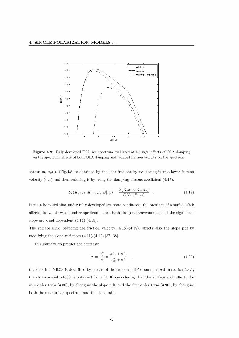
4. SINGLE-POLARIZATION MODELS . . .
Figure 4.8: Fully developed UCL sea spectrum evaluated at 5.5 m/s, effects of OLA damping
on the spectrum, effects of both OLA damping and reduced friction velocity on the spectrum.
spectrum, Sc(·), (Fig.4.8) is obtained by the slick-free one by evaluating it at a lower friction
velocity (u∗c) and then reducing it by using the damping viscous coefficient (4.17):
Sc(K,x, s,Ko, u∗c, |E|, ϕ) =S(K,x, s,Ko, u∗)C(K, |E|, ϕ)
. (4.19)
It must be noted that under fully developed sea state conditions, the presence of a surface slick
affects the whole wavenumber spectrum, since both the peak wavenumber and the significant
slope are wind dependent (4.14)-(4.15).
The surface slick, reducing the friction velocity (4.18)-(4.19), affects also the slope pdf by
modifying the slope variances (4.11)-(4.12) [37; 38].
In summary, to predict the contrast:
∆ =σofσoc
=σo0f + σo1fσo0c + σo1c
, (4.20)
the slick-free NRCS is described by means of the two-scale BPM summarized in section 3.4.1,
the slick-covered NRCS is obtained from (4.10) considering that the surface slick affects the
zero order term (3.86), by changing the slope pdf, and the first order term (3.96), by changing
both the sea surface spectrum and the slope pdf.
82

4.4 A two-scale BPM contrast model
Parameters Value
wind speed 5.7m/swind direction 16North
sea temperature 26.4Cradar frequency 1.25 GHz (L-band) 5.3 GHz (C-band)
radar polarization VV|E| 0.0255N/mϕ -175
β 0.7
Table 4.4: Environmental, radar and OLA parameters used for predicting the contrast.
4.4.3 Experiments and discussion
The effectiveness of the proposed approach is here discussed by showing and analyzing some
meaningful experiments.
First of all the proposed model is employed to predict the contrast due to an Oleyl Alcohol
(OLA) slick, which is commonly used to simulate biogenic slicks [55]. The environmental and
the rheological parameters used, shown in Table 4.4, are the ones relevant to the controlled
experiment described in [51; 55]
In order to better analyze the results, first each term of (4.10) is separately plotted for both
slick-free and slick-covered sea surface, versus the incidence angle.
In Fig.4.9(a) the zero order term (3.86) is shown. It must be noted that for near nadir looking
incidence angles the slick-covered NRCS is larger than the slick-free one. This is due to the fact
that the surface slick, reducing the ripples on the tangent plane, makes the effective Fresnel
coefficient (3.85) larger than the slick-free one, and thus increases the specular reflection. As
far as the incidence angle increases, the NRCS decreases sharply due to the low probability
of having a specular reflection for incidence angles far from nadir. Moreover, the slick-covered
NRCS is smaller than the slick-free one, since the surface slick affects the slope pdf, indirectly,
by means of the slope variances related to the long-wave part of the sea surface spectrum, see
(4.11)-(4.12). To quantitatively analyze such effects Kp, σ2sl,U and σ2
sl,C have been evaluated
for both the slick-free and the slick-covered case. Analysing the results, shown in Table 4.5,
it can be noted that the presence of the surface slick reduces both the peak wavenumber and
the slope variances. These results agree with the ones reported in [56]. However, due to the
limited fetch conditions which characterized wave tank experiments, the reduction of the peak
83

4. SINGLE-POLARIZATION MODELS . . .
Figure 4.9: Comparison between the slick-free and slick-covered NRCS versus the incidence
angle: zero order term (a), first order term (b), total NRCS (c). Contrast referred to the total
(continuous line) and the first order (dashed line) NRCS (d).
84

4.4 A two-scale BPM contrast model
slick-free slick-covered
Kp 0.0048 0.0021σ2sl,U 0.013 0.009σ2sl,C 0.010 0.006kσz 0.116 0.097Kl 42.735 40.515δ 0.385 0.365
Table 4.5: Slick-free and slick-covered electromagnetic and spectrum parameters.
wavenumber and the slope variances experienced in [56] is stronger than the one experienced
in open ocean campaigns [51] and in the experiments reported herein.
In Fig.4.9(b) the first order term (3.96) is shown. Note that to emphasize the variations
the vertical scale is different with respect to the zero order term. For incidence angles larger
than 20 the NRCS decreases with the incidence angle. Moreover, the slick-covered NRCS is
smaller than the slick-free one. This is due to the effects of the surface slick on both the slope
pdf and the small-scale sea surface spectrum, since the first order term can be considered as
a convolution between the latter ones (3.97). As a matter of fact, the surface slick, reducing
the large-scale slopes, makes the range of Bragg wavenumbers over which the averaging (3.96)
takes place smaller. Moreover, the surface slick, reducing the small-scale sea surface spectrum,
reduces the spectral power density of the Bragg waves and therefore leads to a reduction of the
mean backscattered power. To quantitatively analyze the effects of the slick on the small-scale
sea surface spectrum the normalized height variance, kσz, has been evaluated for both the
slick-free and the slick-covered case, see Table 4.5.
It can be noted that, due to the weak damping properties of the OLA slick, the slick-covered
kσz is slightly smaller than the slick-free one. A similar result has been obtained in wave tank
experiments in [56] where, however, the mean surface elevation was strongly reduced by the
surface slick, due to the different environmental conditions [56].
The total contrast (continuous line) and the first order one (dashed line) are shown in Fig.4.9(d).
It can be noted that the total contrast is not given by single terms contrast and the values
predicted by the model, in the typical radar incidence angles (20-60 degrees) range, are around
3dB. This result is in total agreement to what unanimously observed under low to moderate
wind conditions, e.g. [51; 55]. Moreover, for incidence angles larger than 26, the total contrast
is due to the first order term.
85

4. SINGLE-POLARIZATION MODELS . . .
Figure 4.10: C-Band SAR data, p.n. 41370, in which an OLA is present. The dotted lines
show the five transects taken for measuring the contrast (a). Comparison between the predicted
contrast, evaluated according the two-scale BPM (3 dB) and the untilted SPM (13.1 dB), and the
measured contrast (mean contrast 3.1 dB), both at L- and C-band for incidence angles ranging
between 29.3and 29.7.
A tailored analysis on the effects of a biogenic slick on the limit wavenumber (4.16) has
been accomplished [37]. Results, shown in Table 4.5, witnesses a shift of Klim towards lower
wavenumbers and a δ value within the recommended range 0.3-0.5 (section 3.4.1). This result,
confirms the theoretical predictions and, per se, demonstrates that in presence of biogenic slick
the Bragg scattering applies. This has important applicative consequences even beyond the
model presented in this study [37].
In order to further validate the new contrast model, independent experiments on the same
data set used in [51] have been accomplished. The predicted VV L- and C-band contrast,
evaluated by using both the two-scale BPM approach and the untilted SPM one, in which
only the pure Marangoni damping is taken into account, has been compared to the contrast
measured on real SAR data. In detail, five transects at different incidence angles, ranging
between 29.3and 29.7, have been taken along with the VV L- and C-band multi-look complex
(MLC) SIR-C/X-SAR images, acquired on 1 October 1994, 5:33 UTC (processing numbers
(pn) 41369 and 41370, respectively), in which OLA slicks are present. Such data have been
acquired during a controlled experiment in which both the environmental conditions and the
rheological parameters of the spilled OLA were known [51; 55], see Table 4.4. In Fig.4.10(a)
the VV C-band SAR data, in which the OLA is clearly visible, is shown. In Fig.4.10(b), the
two-scale BPM total contrast (solid line) and the first order BPM contrast (dotted dashed line)
86
4.5 Conclusions
are plotted versus the Bragg wavenumber, for reference purposes the untilted SPM contrast is
also shown (dotted line). Stars represent real data measurements. Analysing the results shown
in Fig.4.10(b), it must be noted that the total BPM contrast, for the incidence angles used in
this experiment, is only due to the first order term. This result is in perfect agreement to what
experienced in [56] in which a three-scale scattering model was used to explain results obtained
in wave tank experiments.
Moreover, Fig.4.10(b) clearly show a remarkable agreement of the two-scale BPM contrast with
real data and a very poor behaviour of the untilted SPM contrast. A discrepancy of about 8
dB is experienced at C-band! This clearly confirm the result of [51; 55] and suggest that an
enhancement of the contrast modelling is necessary.
In summary theoretical and real data experiments, based on direct and indirect measure-
ments, shown that:
• the classical untilted SPM associated to the pure Marangoni damping is not able to predict
the biogenic contrast;
• the two-scale BPM contrast model associated to the pure Marangoni damping is able to
reasonably predict the biogenic contrast.
Actually, the first result is not new, as clearly stated for instance in [55]. The novelty is that,
although it was clear that an enhancement of the contrast modelling was necessary, in [51; 54]
the enhancement was only meant in terms of enhancement of the Marangoni damping model,
while in this paper it has been shown that an appropriate sea scattering model is also a key
issue.
4.5 Conclusions
In this section, starting from the theoretical background developed in chapter 3, new single
polarization electromagnetic models have been developed and specialized to describe sea surface
scattering mechanism with and without surface slicks.
It has been shown that speckle, which is commonly meant to hamper SAR image inter-
pretability and, therefore, reduced by degrading the available spatial resolution, once properly
modelled by means of the GK pdf, is a source of information. In fact, the three GK parameters
allow emphasizing, in full resolution SAR data, the peculiarities of the sea surface scattering
which occurs when low backscatter areas or small dominant scatters are in place.
87

4. SINGLE-POLARIZATION MODELS . . .
This theoretical model has been shown to be very useful, from an operational viewpoint, in
SAR sea oil slick detection procedures. It must be explicitly noted that, unlike classical oil
slick detection procedures which, based on pure image processing techniques, do not allow un-
derstanding the underpinning physic at the problem basis, the electromagnetic approach, since
based on a tailored electromagnetic modelling of the sea surface scattering mechanism, allows
recognizing that, if single polarization SAR data are available, in general, it is not possible dis-
tinguishing among the different phenomena which generate low backscatter areas. This latter
point can be addressed only by means of ancillary information, e.g. wind speed.
Moreover, the proposed electromagnetic approach can be very helpful dealing with this latter
aspect. In fact, since it is able to detect simultaneously both small dominant scatters (e.g.
ships) and low backscatter areas, the proposed approach allows correlating the presence of a
ship to a low backscatter area. This makes the probability that the low backscatter area is due
to an oil slick very high.
Following a guideline similar to the one above described, an electromagnetic approach has
been proposed to detect ships in single-polarization SAR data.
Unlike classical SAR ship detection procedures which, based on image processing techniques,
operate taking into account the typical features which a ship makes in SAR images, the proposed
approach is based on the effects which a ship has on the sea surface scattering mechanism. In
particular, the ship is read in terms of the strong and coherent backscattering which it calls
for. Following this theoretical rationale a filter, which is able to operate on full resolution SAR
data, has been developed. The filter has been shown to be both computer time effective and
characterized by a low false alarm rate.
Finally, since one of the main open issues in SAR sea oil slick detection is classificating the
detected dark areas in terms of oil slicks and considering that one of the main important look
alike is due to biogenic slicks, a study on the sea surface scattering with and without biogenic
slicks has been accomplished.
The study, aimed at developing a model for predicting the contrast due to a biogenic slick, has
demonstrated the importance of a proper electromagnetic description of the slick-free sea surface
scattering. In fact, unlike classical approaches which, based on the SPM scattering model, are
not able to well predict the contrast measured in presence of a biogenic slick, the proposed
approach, based on a two-scale sea surface scattering model shows a remarkable agreement
with the measured contrast.
This study is also important from an operational viewpoint in dark area detection procedures
88

4.5 Conclusions
since it allows evaluating a physically consistent threshold, instead of the classical empirical
threshold commonly employed.
89

4. SINGLE-POLARIZATION MODELS . . .
90
5
Multi-polarization model for sea
oil slick observation
5.1 Introduction
Physically SAR sea oil slick observation is possible since an oil slick, damping the short waves
responsible for the signal backscattered to the receiving antenna, generates a low backscatter
area. Following this physical rationale, in the previous chapter, single-polarization electromag-
netic models have been developed and shown to be mainly useful for dark area detection in
SAR images.
However, it is well-known that, due to the presence of oil look-alike, SAR oil slick observation
cannot be accomplished by simply detecting dark areas in SAR images. Generally, ancillary
data (e.g. wind speed) or information about the observed scene gathered by other sensors (e.g.
optical sensors) are exploited [64].
In this chapter, which represents the main second innovative contribute to the thesis, start-
ing from the theoretical background presented in chapter 2, the vectorial nature of the scattered
field, i.e. its polarization properties, is taken into account to develop a polarimetric electromag-
netic model aimed at both observing oil slicks and distinguishing them from one of the most
important look alike, i.e. biogenic slicks. In fact, in this chapter it is demonstrated that, oil
and biogenic slicks not only generate different contrasts but even different polarimetric features
which can be distinguished once a proper electromagnetic multi-polarization model is available.
This fact represents a new scientific paradigm which opens a brand new view of the problem.
In fact, although in literature there is a general consensus that radar polarimetry is able to
91
5. MULTI-POLARIZATION MODEL. . .
provide additional information to environmental applications, the real benefit of SAR polari-
metric information, which can be extracted once a proper electromagnetic model is available,
was demonstrated only for land applications and first investigations on sea oil slick observation
were generally unsatisfactory [51]. Only recently it was shown that fully polarimetric data can
be usefully employed to assist classical oil slick observation procedures [65].
In this chapter a polarimetric scattering model able to describe the sea surface scattering
with and without surface slicks is firstly developed, under low to moderate wind conditions.
Such a model is then specialized for the practical cases in which fully-polarimetric or dual-
polarimetric SAR data are available. The content of this chapter is based on paper published
or submitted to international journals and presented at international conferences [66; 67; 68; 69].
The chapter is organized as follows. In section 5.2, the general polarimetric scattering
model is developed for predicting slick-free and slick-covered sea surface scattering, under low
to moderate wind conditions. In section 5.3, the usefulness of fully polarimetric SAR data is
investigated by considering two approaches. In the first one, the co-polarized signature, which
in [51] has been considered unsatisfactory for oil slick observation, is shown to have a different
sensitivity with respect to oil and biogenic slicks, which can be exploited both for observing
sea oil slicks and for distinguishing them from biogenic look alike. The second approach is
based on the Mueller matrix which is used to develop a filtering technique which is shown to
be operationally interesting since its true-false logical output clearly shows the presence of oil
slicks. In section 5.4, the usefulness of dual-polarimetric SAR data is investigated by using
an approach based on the phase difference between the complex HH and VV channels. The
approach is shown to be able to emphasize the presence of an oil slick and to de-emphasize
biogenic slicks.
5.2 The polarimetric model
The scattering matrix S relates the electromagnetic field scattered by the observed scene to the
incident one according to the Jones formalism, see section 2.5.1:
Es =e−jkr
rSEi . (5.1)
Once S has been measured, the Mueller matrix can be constructed. It relates the Stokes vector
scattered by the observed scene, ss, to the incident one, si, (2.92):
ss = (kr)−2〈M〉si . (5.2)
92

5.2 The polarimetric model
Since it is able to describe also partially polarized scattered fields (5.2) is the most general way
to deal with polarimetric surface scattering, see section 2.5.2. Moreover, the Mueller matrix
plays a fundamental role in electromagnetic modelling of polarimetric surface scattering since
it is the only means available for comparing measured data with theoretical models. In fact,
scattering models for distributed targets are inherently ensemble-average processes and their
outputs products are expression of the Mueller matrix. The wave scattered by the observed
scene is generally partially polarized and, thus, can be decomposed into its fully-polarized and
fully-unpolarized components, see section 2.3:
ss = ssP + ssU . (5.3)
To investigate the polarimetric sea surface scattering mechanism with and without surface
slicks, under low to moderate wind conditions, some reference scenarios must be distinguished.
In the case of slick-free sea surface, the small-scale scattering is well-modelled by the Bragg
scattering which is a single scattering mechanism. It is characterized by a low polarimetric
entropy [65] and, since the polarimetric entropy is a measure of the degree of randomness of the
scattering mechanism, by a low unpolarized backscattered energy and by an high correlation
between the HH and VV complex channels [66; 67].
In the case of slick-covered sea surface, due to their different damping properties two cases
must be considered.
In the case of oil-covered sea surface, due to the strong damping properties of oil slicks, a low
backscattered signal and a high polarimetric entropy, which suggests a non-Bragg scattering
mechanism, are expected and demonstrated [65; 66; 67]. The high polarimetric entropy wit-
nesses that a complex scattering mechanism is in place [17], which is characterized by a large
amount of unpolarized backscattered energy and by a low correlation between the HH and VV
complex channels [66; 67].
Completely different is the case of a biogenic-covered sea surface. In fact, due to the weak
damping properties of biogenic slicks [55], the scattering mechanism still calls for a Bragg one,
but characterized by a low backscattered signal. Hence, this case, in terms of polarimetric
scattering mechanism, is expected to be indistinguishable from the one relevant to the slick-free
sea surface.
As a matter of fact, in case of oil-covered sea surface, the polarimetric model predicts a scat-
tering behaviour completely different from the slick-free sea surface while, in case of biogenic-
covered sea surface, the polarimetric scattering behaviour is expected to be indistinguishable
93

5. MULTI-POLARIZATION MODEL. . .
slick-free & biogenic covered sea surface oil-covered sea surface
Bragg scattering non-Bragg scatteringlow polarimetric entropy high polarimetric entropylow unpolarized energy high unpolarized energyhigh HH-VV correlation low HH-VV correlation
Table 5.1: Polarimetric sea surface scattering mechanism with and without surface slicks.
from the slick-free one.
To better emphasize the model prediction the key scattering features which characterize the
slick-free (and biogenic-covered) and oil-covered sea surface cases are summarized in Table 5.1.
Following this theoretical rationale, in the next sections, a set of polarimetric approaches are
developed which are demonstrated to be useful for oil slick detection purposes. Though these
approaches are based on the general polarimetric model above developed and summarized in
Table 5.1, from an operational viewpoint, it is useful to sort them according to the kind of
polarimetric data they need. Accordingly, they are classified in fully polarimetric approaches,
i.e. the whole scattering matrix is needed, dual polarimetric approaches, i.e. two terms of the
scattering matrix are needed.
5.3 Fully polarimetric approaches
A fully polarimetric SAR measures the scattering matrix for each resolution cell. Provided S,
the Mueller matrix and the Kennaugh matrix can be constructed. In this section, the theoretical
model previously developed is specialized to observe sea oil slick in fully polarimetric SAR data.
In particular two approaches are presented and discussed by considering two reference cases,
well-detailed in literature [51], relevant to fully polarimetric MLC SAR data acquired, under
low to moderate wind conditions, during the mission SIR-C/X-SAR.
The first data is relevant to the acquisition of 1 October 1994, 8:14 UTC, processing number
(p.n.) 44327, in which an oil slick is present. The second data is relevant to the acquisition of 1
October 1994, 5:33 UTC, p.n. 41370, in which an OLA is present. OLA forms a monomolecular
surface film which well simulates a biogenic surface slick [51].
94

5.3 Fully polarimetric approaches
5.3.1 Polarization Signature
Polarization signature [14; 70], which consists of a plot of synthesized NRCS as a function of
the ellipticity and orientation angles of the co-polarized and cross-polarized transmitting and
receiving antenna, is an important tool in remote sensing applications. In fact, the shape of
the plots and the pedestal on which the polarization signature is set provide information about
the dominant scattering mechanism [71; 72] which can be usefully employed for classification
purposes.
Polarization signatures have been successfully employed to classify a wide range of terrain
types according to their different polarimetric scattering properties [72; 73]. Dealing with sea
applications, polarization signatures have been employed in [71] to investigate the effects of
long waves tilting in polarimetric sea surface scattering. First experimental investigations on
sea oil slick observation have been considered unsatisfactory [51].
In this section, a new physical approach in which, following the theoretical model previously
developed, the polarization signature is read in terms of sea surface scattering mechanism with
and without surface slicks is proposed. Accordingly, a filtering technique which is able to both
observe oil slicks and distinguish them from biogenic slicks in fully polarimetric SAR data, is
described and discussed by means of some meaningful experiments.
Further details can be found in [68; 69].
5.3.2 Pedestal height for oil slick observation
Polarization synthesis techniques, see section 2.5.3, allow evaluating the scattering coefficient
for any possible combination of transmitting and receiving antenna polarizations, by using the
Kennaugh matrix: [14; 70]:
σoχ,ψ =12
4πk2
sr(T )Kst , (5.4)
where the normalized Stokes vectors which describe the transmitting and receiving antenna
properties are expressed in terms of the correspondent ellipticity and orientation angle:
st(r) =
1
cos 2χt(r) cos 2ψt(r)cos 2χt(r) sin 2ψt(r)
sin 2χt(r)
(5.5)
The polarimetric information contained in (5.4) is generally displayed as a 3D plot, called
polarization signature, for identical (co-polarized signature) and orthogonal (cross-polarized
signature) transmitting and receiving antenna polarizations [70].
95

5. MULTI-POLARIZATION MODEL. . .
In this study, the co-polarized signature is read in terms of sea surface scattering with and
without surface slicks. Following the theoretical rationale developed in section 5.2 and consid-
ering that the pedestal height is related to the amount of unpolarized backscattered energy 5.3,
the pedestal is expected to be both able to detect sea oil slick and useful to distinguish them
from biogenic look-alike.
In detail, in case of slick-free sea surface, since a Bragg scattering mechanism is in place, a
co-polarized signature characterized by a maximum at vertical polarization, a saddle point at
horizontal polarization and two nulls at elliptical polarization, is expected [70]. Moreover, since
slick-free sea surface can be considered as a natural surface with low depolarizing capabilities,
a low unpolarized backscattered energy is expected.
In case of oil-covered sea surface, due to the strong damping properties of oil slicks, an high
unpolarized backscattered energy and, therefore, a pedestal height larger than the slick-free sea
surface one is expected.
In case of biogenic-covered sea surface, due to the weak damping properties of biogenic slicks,
the pedestal height is expected to be indistinguishable to the one relevant to the surrounding
slick-free sea surface, see Table 5.1.
In summary, the model predicts a pedestal height sensitive to the polarimetric scattering with
and without surface slicks. Moreover, due to their completely different damping properties, the
pedestal height should be able to both observe sea oil slicks and distinguish them from biogenic
slicks.
5.3.3 Experiments
In this paragraph some meaningful experiments, accomplished on the data set detailed in sec-
tion 5.1, are presented and discussed to demonstrate the capability of the co-polarized signature
both to observe oil slicks and to distinguish them from biogenic look-alike.
Fig.5.1 shows an excerpt of the C-band VV power SAR image in which an oil slick is
clearly visible. The normalized co-polarized signature has been evaluated for both the oil-free
(Fig.5.2(a)) and the oil-covered (Fig.5.2(b)) sea surface, by considering two region of interest
(ROI) of equal size. By comparing the two polarization signatures it can be noticed that, as
predicted in the previous section, the oil slick, increasing the amount of unpolarized backscat-
tered energy, makes the pedestal higher. It must be noted that the increase of the pedestal is
not related to the low SIR-C signal to noise ratio (SNR), which is -28dB, since the oil-covered
polarization signature has been computed considering the pixel values above the SIR-C noise
96

5.3 Fully polarimetric approaches
Figure 5.1: VV power image relevant to the acquisition of 1 October 1994, 8:14 UTC p.n. 44327.
Figure 5.2: Slick-free (a) and slick-covered (b) co-polarized polarization signatures.
floor. Since the pedestal height seems to be a good feature for observing oil slicks, a tailored
filtering technique for estimating the pedestal height by SAR polarimetric data has been devel-
oped. The estimated pedestal, relevant to the first data set, is shown in grey tones in Fig. 5.3. It
can be noticed that the filtering technique emphasizes the presence of the oil slick with respect
to the surrounding sea, if compared to the VV power image shown in Fig.5.1.
Fig.5.4 shows an excerpt of the C-band VV power SAR image in which the OLA slick is
clearly visible. The normalized co-polarized signature, evaluated for both the slick-free and the
slick-covered sea surface are shown in Figs.5.5(a)-(b).
The two co-polarized signatures are indistinguishable. This result confirms the proposed the-
oretical model which predicts, for a weaker damping, a scattering mechanism similar to the
97
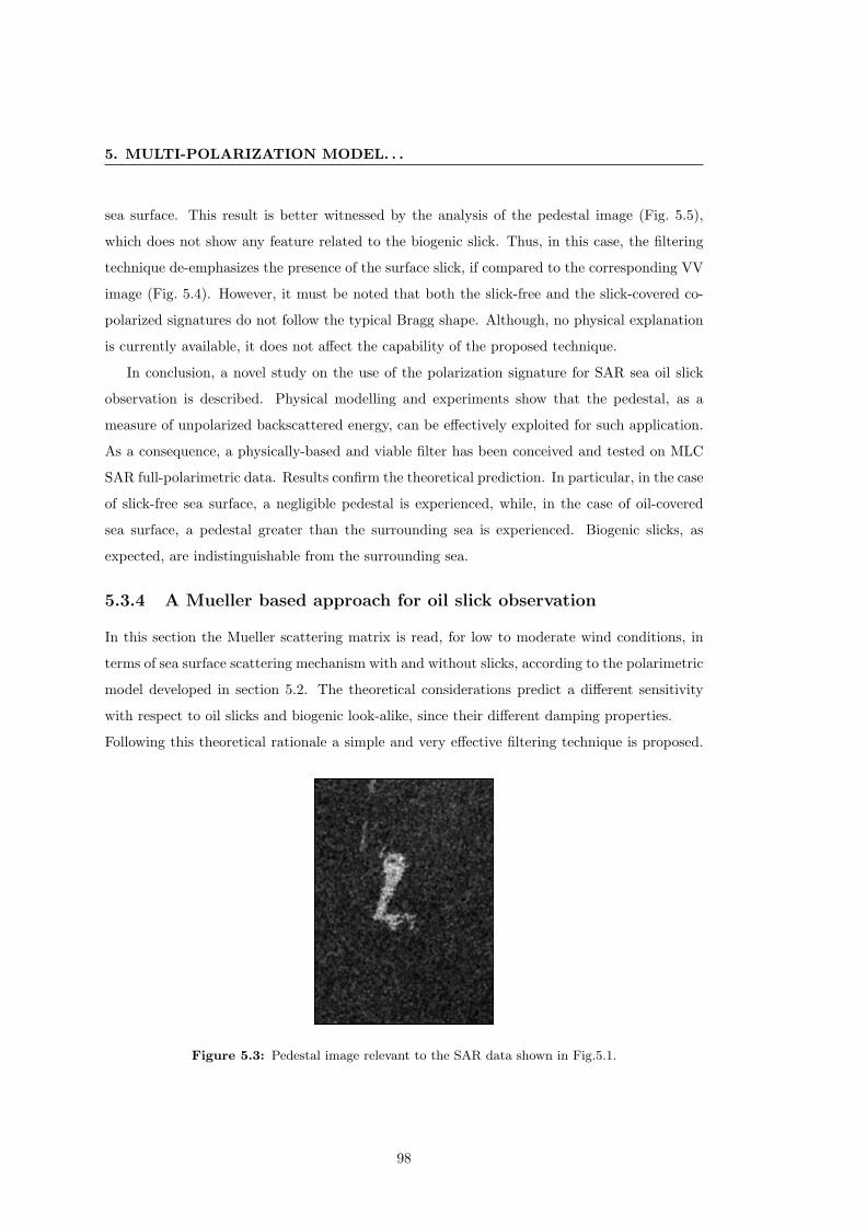
5. MULTI-POLARIZATION MODEL. . .
sea surface. This result is better witnessed by the analysis of the pedestal image (Fig. 5.5),
which does not show any feature related to the biogenic slick. Thus, in this case, the filtering
technique de-emphasizes the presence of the surface slick, if compared to the corresponding VV
image (Fig. 5.4). However, it must be noted that both the slick-free and the slick-covered co-
polarized signatures do not follow the typical Bragg shape. Although, no physical explanation
is currently available, it does not affect the capability of the proposed technique.
In conclusion, a novel study on the use of the polarization signature for SAR sea oil slick
observation is described. Physical modelling and experiments show that the pedestal, as a
measure of unpolarized backscattered energy, can be effectively exploited for such application.
As a consequence, a physically-based and viable filter has been conceived and tested on MLC
SAR full-polarimetric data. Results confirm the theoretical prediction. In particular, in the case
of slick-free sea surface, a negligible pedestal is experienced, while, in the case of oil-covered
sea surface, a pedestal greater than the surrounding sea is experienced. Biogenic slicks, as
expected, are indistinguishable from the surrounding sea.
5.3.4 A Mueller based approach for oil slick observation
In this section the Mueller scattering matrix is read, for low to moderate wind conditions, in
terms of sea surface scattering mechanism with and without slicks, according to the polarimetric
model developed in section 5.2. The theoretical considerations predict a different sensitivity
with respect to oil slicks and biogenic look-alike, since their different damping properties.
Following this theoretical rationale a simple and very effective filtering technique is proposed.
Figure 5.3: Pedestal image relevant to the SAR data shown in Fig.5.1.
98
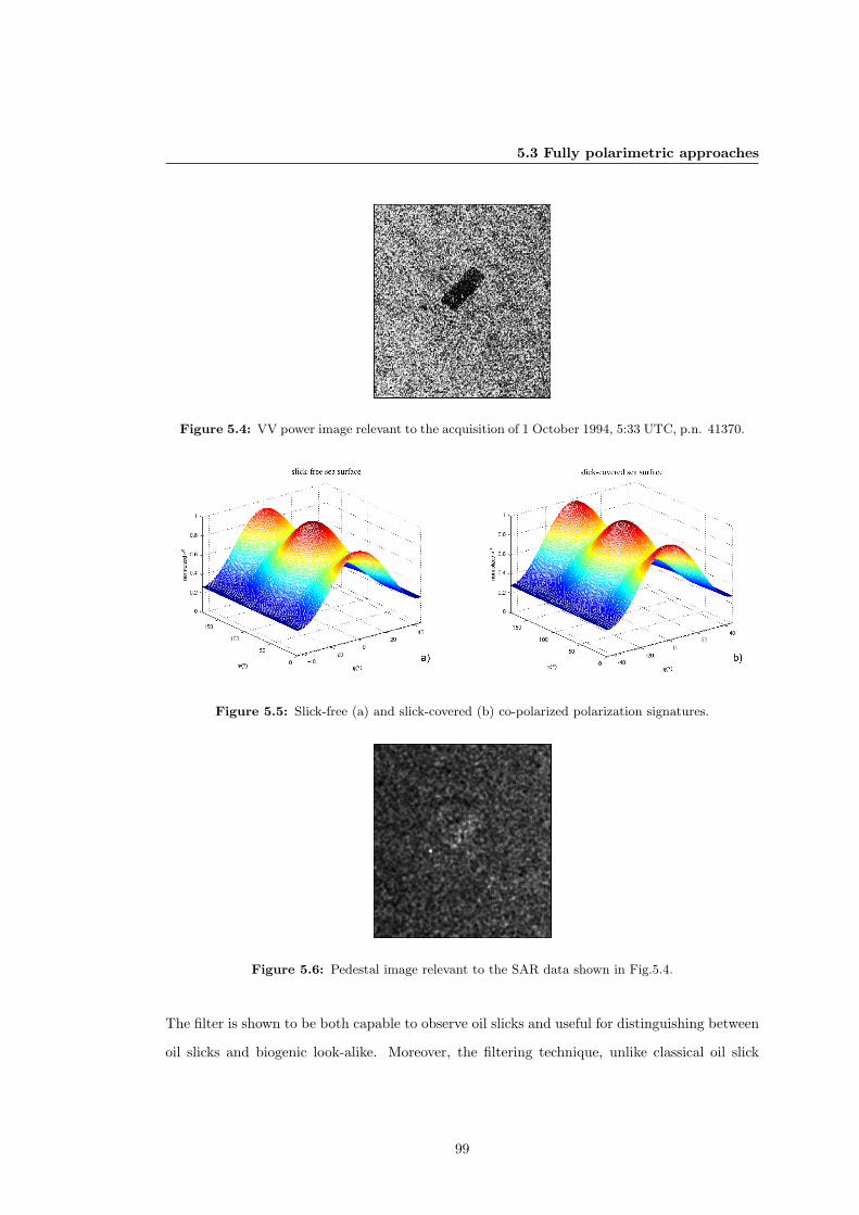
5.3 Fully polarimetric approaches
Figure 5.4: VV power image relevant to the acquisition of 1 October 1994, 5:33 UTC, p.n. 41370.
Figure 5.5: Slick-free (a) and slick-covered (b) co-polarized polarization signatures.
Figure 5.6: Pedestal image relevant to the SAR data shown in Fig.5.4.
The filter is shown to be both capable to observe oil slicks and useful for distinguishing between
oil slicks and biogenic look-alike. Moreover, the filtering technique, unlike classical oil slick
99

5. MULTI-POLARIZATION MODEL. . .
observation techniques, which are generally based on thresholding procedures [34], does not
need any threshold.
Further details can be found in [67].
5.3.5 The fully-polarimetric Mueller filter
Dealing with sea surface scattering, due to the low correlation between the co- and cross-
polarized channels [74], the Mueller matrix presents only eight non-zero elements [16], which
can be written in terms of the scattering amplitudes Sxy, with x, y = h, v:
M =
A+Bo B 0 0B A−Bo 0 00 0 C +Bo D0 0 −D C −Bo
, (5.6)
where [75]:
A =12〈|Shh|2 + |Svv|2〉 , (5.7)
B =12〈|Shh|2 − |Svv|2〉 , (5.8)
Bo = 〈|Shv|2〉 , (5.9)
C = 〈<(ShhS∗vv)〉 , (5.10)
D = 〈=(ShhS∗vv)〉 , (5.11)
Note that A, B, C and D are related to the co-polarized scattering amplitudes while Bo is
related to the cross-polarized one.
To read the Mueller matrix in terms of the slick-free and slick-covered sea surface scattering
mechanism, reference is made to C and Bo. In fact, C is related to the correlation between the
complex HH and VV channels while Bo is related to the cross-polarized backscattered energy.
As a matter of fact, following the theoretical rationale developed in section 5.2, in case of
slick-free sea surface a Bragg scattering mechanism characterized by a low polarimetric entropy
is in place. This means that an high correlation between the HH and VV channels and a low
cross-polarized backscattered energy are to be expected. Accordingly, the following relationship
holds:
|C| > Bo . (5.12)
In the case of oil-covered sea surface, the high entropy which characterizes the non-Bragg
scattering mechanism makes the HH and VV channels practically uncorrelated [66]. As a
100
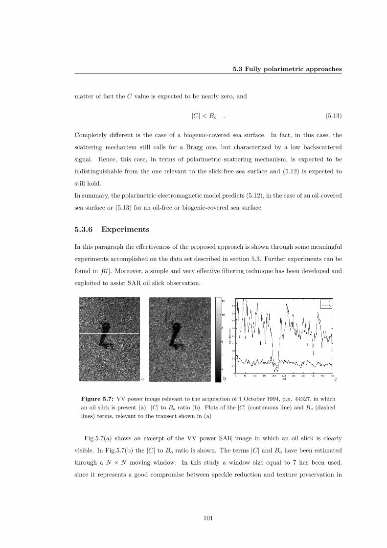
5.3 Fully polarimetric approaches
matter of fact the C value is expected to be nearly zero, and
|C| < Bo . (5.13)
Completely different is the case of a biogenic-covered sea surface. In fact, in this case, the
scattering mechanism still calls for a Bragg one, but characterized by a low backscattered
signal. Hence, this case, in terms of polarimetric scattering mechanism, is expected to be
indistinguishable from the one relevant to the slick-free sea surface and (5.12) is expected to
still hold.
In summary, the polarimetric electromagnetic model predicts (5.12), in the case of an oil-covered
sea surface or (5.13) for an oil-free or biogenic-covered sea surface.
5.3.6 Experiments
In this paragraph the effectiveness of the proposed approach is shown through some meaningful
experiments accomplished on the data set described in section 5.3. Further experiments can be
found in [67]. Moreover, a simple and very effective filtering technique has been developed and
exploited to assist SAR oil slick observation.
Figure 5.7: VV power image relevant to the acquisition of 1 October 1994, p.n. 44327, in which
an oil slick is present (a). |C| to Bo ratio (b). Plots of the |C| (continuous line) and Bo (dashed
lines) terms, relevant to the transect shown in (a)
Fig.5.7(a) shows an excerpt of the VV power SAR image in which an oil slick is clearly
visible. In Fig.5.7(b) the |C| to Bo ratio is shown. The terms |C| and Bo have been estimated
through a N × N moving window. In this study a window size equal to 7 has been used,
since it represents a good compromise between speckle reduction and texture preservation in
101

5. MULTI-POLARIZATION MODEL. . .
Figure 5.8: VV power image relevant to the acquisition of 1 October 1994, p.n. 41370, in which
an OLA is present (a). |C| to Bo ratio (b). Plots of the |C| (continuous line) and Bo (dashed
lines) terms, relevant to the transect shown in (a)
polarimetric SAR images [76]. The analysis of this image witnesses that (5.13) holds for oil-
covered sea surface while (5.12) for the surrounding oil-free sea surface. To further support this
result, |C| and Bo values, estimated along with the transect shown in Fig.5.7(a), are plotted
together in Fig.5.7(c). It can be noted that |C| and Bo are always well-separated except within
the oil-covered sea surface, where (5.13) holds. These results, together with the oil-covered and
oil-free polarimetric entropy (0.89 and 0.61, respectively), estimated according to [17], confirm
the theoretical model proposed in the previous section, which predicts a different scattering
mechanism in presence of an oil slick.
Fig.5.8(a) shows an excerpt of the VV power SAR image in which an OLA slick is clearly visible.
The analysis of the |C| to Bo ratio image (Fig.5.8(b)) witnesses that (5.12) holds both for the
slick-free and the slick-covered sea surface, as highlighted by the analysis of the |C| and Bo
values, which are always well-separated (Fig. 5.8(c)). This result and the estimated polarimetric
entropy values, which are 0.54 and 0.53 for the slick-covered and slick-free sea surface, confirm
the proposed theoretical model which predicts, for a weaker damping, a scattering mechanism
similar to the sea surface.
The theoretical rationale previously developed and the experiments shown suggest a simple
and very effective filtering technique, which can assist SAR oil slick observation.
The filter simply compares the terms |C| and Bo and assigns a logical value which is coded in
two colors: black if (5.13) holds and white if (5.12) holds.
In Fig.5.9(a-b) two meaningful results, obtained applying the filter to the first data set, in which
an oil slick is present (Fig.5.7(a)), and to the second data set, in which an OLA is present
102
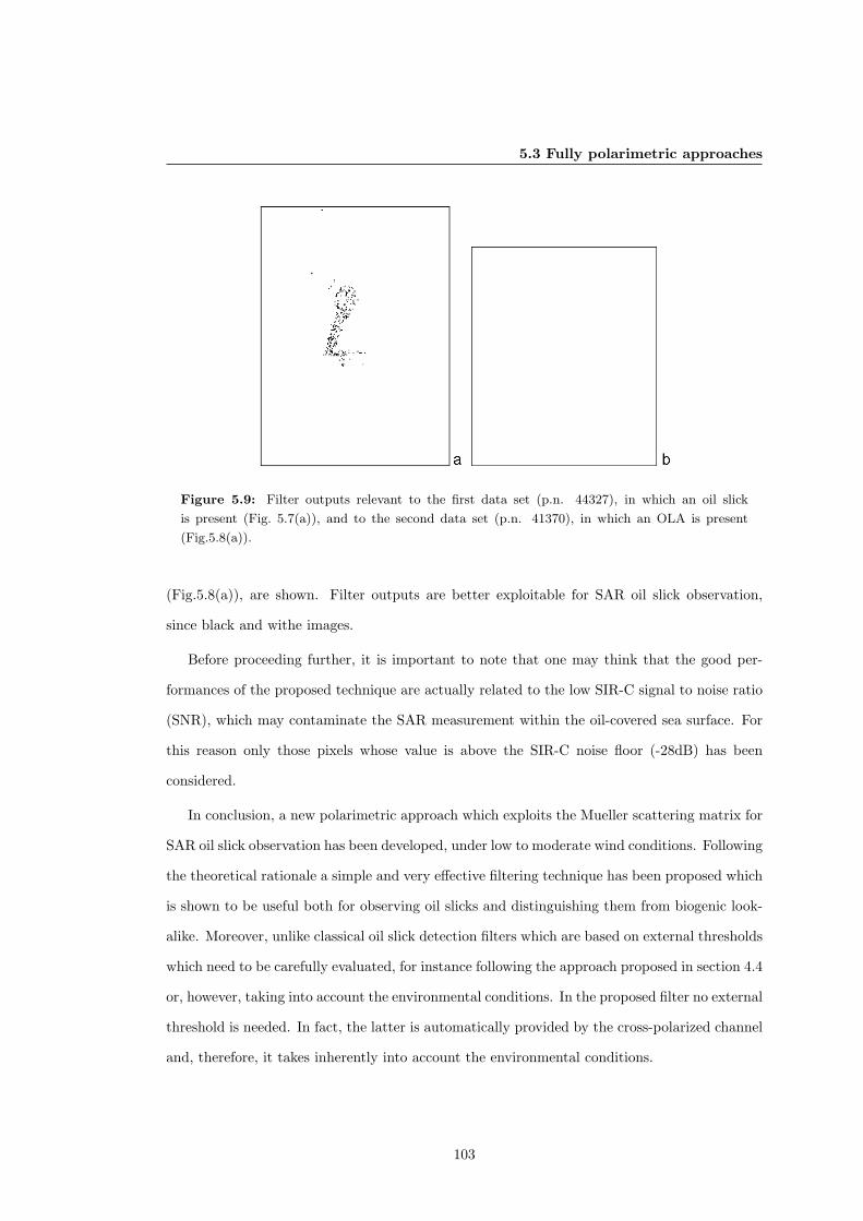
5.3 Fully polarimetric approaches
Figure 5.9: Filter outputs relevant to the first data set (p.n. 44327), in which an oil slick
is present (Fig. 5.7(a)), and to the second data set (p.n. 41370), in which an OLA is present
(Fig.5.8(a)).
(Fig.5.8(a)), are shown. Filter outputs are better exploitable for SAR oil slick observation,
since black and withe images.
Before proceeding further, it is important to note that one may think that the good per-
formances of the proposed technique are actually related to the low SIR-C signal to noise ratio
(SNR), which may contaminate the SAR measurement within the oil-covered sea surface. For
this reason only those pixels whose value is above the SIR-C noise floor (-28dB) has been
considered.
In conclusion, a new polarimetric approach which exploits the Mueller scattering matrix for
SAR oil slick observation has been developed, under low to moderate wind conditions. Following
the theoretical rationale a simple and very effective filtering technique has been proposed which
is shown to be useful both for observing oil slicks and distinguishing them from biogenic look-
alike. Moreover, unlike classical oil slick detection filters which are based on external thresholds
which need to be carefully evaluated, for instance following the approach proposed in section 4.4
or, however, taking into account the environmental conditions. In the proposed filter no external
threshold is needed. In fact, the latter is automatically provided by the cross-polarized channel
and, therefore, it takes inherently into account the environmental conditions.
103

5. MULTI-POLARIZATION MODEL. . .
5.4 Dual-polarimetric approach
Although a fully polarimetric SAR is to be desired, there may be hardware and budget consid-
erations that can suggest to design and implement a simpler polarimetric SAR configuration.
For instance, the SAR on board of RADARSAT-2 and ALOS PALSAR operate in fully, dual-
and single- polarization modes while the SARs on board of the ENVISAT and the COSMO
SKYMED operate only in single or in dual polarization modes. As the matter of fact, the use
of dual-polarized SAR sensors for oil slick observation is operationally important.
In this section the theoretical model developed in section 5.2 is specialized to observe oil slick in
dual-polarized SAR data. In particular an approach, based on the co-polarized phase difference
(CPD), i.e. the phase difference between the complex HH and VV channels, is presented and
discussed by considering the two reference cases detailed in section 5.3.
5.5 Co-polarized phase difference
Many studies about the capability of partially polarimetric SAR data for geophysical remote
sensing have been addressed, e.g. [77]. Among them, there are some theoretical and land
application studies which employ the CPD (see references cited in [66]). However, only few and
preliminary studies regard sea application of the CPD [71] and no-one oil slick observation.
In this section the CPD, is read in terms of the sea surface scattering mechanism with and
without surface slick, according to the model developed in section 5.2.
It is shown that, under low to moderate wind conditions, the broadening of the CPD pdf is
sensitive to the presence of a low backscattering area. Moreover, the theoretical considerations
predict a different sensitivity of oil and biogenic slicks, since their different damping effects.
Following this theoretical rationale a novel filtering technique, which is shown to be both able
to observe oil slicks and distinguish them from biogenic slicks in dual-polarized SAR data, is
implemented.
Further details can be found in [66]
5.5.1 CPD approach
The scattering matrix, considering for instance the horizontal and vertical linearly polarized
electric fields, can be expressed by:
S =(Svv SvhShv Shh
), (5.14)
104
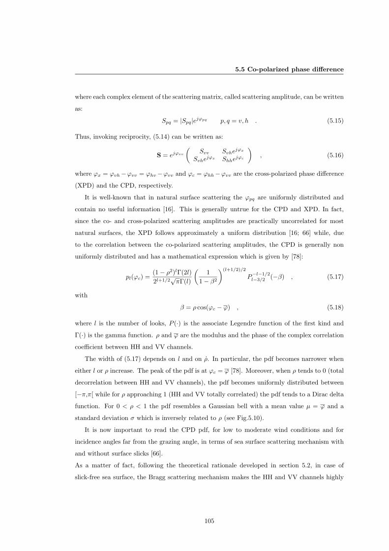
5.5 Co-polarized phase difference
where each complex element of the scattering matrix, called scattering amplitude, can be written
as:
Spq = |Spq|ejϕpq p, q = v, h . (5.15)
Thus, invoking reciprocity, (5.14) can be written as:
S = ejϕvv(
Svv Svhejϕx
Svhejϕx Shhe
jϕc
), (5.16)
where ϕx = ϕvh−ϕvv = ϕhv−ϕvv and ϕc = ϕhh−ϕvv are the cross-polarized phase difference
(XPD) and the CPD, respectively.
It is well-known that in natural surface scattering the ϕpq are uniformly distributed and
contain no useful information [16]. This is generally untrue for the CPD and XPD. In fact,
since the co- and cross-polarized scattering amplitudes are practically uncorrelated for most
natural surfaces, the XPD follows approximately a uniform distribution [16; 66] while, due
to the correlation between the co-polarized scattering amplitudes, the CPD is generally non
uniformly distributed and has a mathematical expression which is given by [78]:
pl(ϕc) =(1− ρ2)lΓ(2l)2l+1/2
√πΓ(l)
(1
1− β2
)(l+1/2)/2
P−l−1/2l−3/2 (−β) , (5.17)
with
β = ρ cos(ϕc − ϕ) , (5.18)
where l is the number of looks, P (·) is the associate Legendre function of the first kind and
Γ(·) is the gamma function. ρ and ϕ are the modulus and the phase of the complex correlation
coefficient between HH and VV channels.
The width of (5.17) depends on l and on ρ. In particular, the pdf becomes narrower when
either l or ρ increase. The peak of the pdf is at ϕc = ϕ [78]. Moreover, when ρ tends to 0 (total
decorrelation between HH and VV channels), the pdf becomes uniformly distributed between
[−π,π[ while for ρ approaching 1 (HH and VV totally correlated) the pdf tends to a Dirac delta
function. For 0 < ρ < 1 the pdf resembles a Gaussian bell with a mean value µ = ϕ and a
standard deviation σ which is inversely related to ρ (see Fig.5.10).
It is now important to read the CPD pdf, for low to moderate wind conditions and for
incidence angles far from the grazing angle, in terms of sea surface scattering mechanism with
and without surface slicks [66].
As a matter of fact, following the theoretical rationale developed in section 5.2, in case of
slick-free sea surface, the Bragg scattering mechanism makes the HH and VV channels highly
105

5. MULTI-POLARIZATION MODEL. . .
Figure 5.10: Plots of the theoretical CPD pdf for |ρ| = 0.1, 0.7, 0.9 and its phase ϕ = 0, with
l = 4
correlated and, therefore, a narrow CPD pdf is to be expected.
In case of oil-covered sea surface, the high entropy which characterizes the non-Bragg scattering
mechanism makes the HH and VV channels practically uncorrelated and, therefore, a broader
CPD pdf is to be expected.
In other words, oil slicks, which are generally characterized by strong damping properties, are
expected to be well-distinguishable from the surrounding sea since their different scattering
mechanisms.
Very much different is the case of a biogenic-covered sea surface. In fact, in this case, the
scattering mechanism still calls for a Bragg one, but characterized by a low backscattered
signal. Therefore, similar CPD pdfs for the slick-free and biogenic-covered sea surface are to
be expected.
5.5.2 Experiments
In this paragraph the effectiveness of the proposed approach is shown through some meaningful
experiments accomplished on the data set described in section 5.3. Further experiments can be
found in [66].
SAR data have been processed by means of a simple and effective filtering technique which,
applied over the CPD image, estimate µ and σ through a N ×N moving window. In this study
106
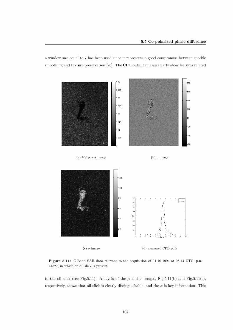
5.5 Co-polarized phase difference
a window size equal to 7 has been used since it represents a good compromise between speckle
smoothing and texture preservation [76]. The CPD output images clearly show features related
(a) VV power image (b) µ image
(c) σ image (d) measured CPD pdfs
Figure 5.11: C-Band SAR data relevant to the acquisition of 01-10-1994 at 08:14 UTC, p.n.
44327, in which an oil slick is present.
to the oil slick (see Fig.5.11). Analysis of the µ and σ images, Fig.5.11(b) and Fig.5.11(c),
respectively, shows that oil slick is clearly distinguishable, and the σ is key information. This
107

5. MULTI-POLARIZATION MODEL. . .
result confirms the theoretical model previously proposed, which predicts a different scattering
mechanism in presence of an oil slick and it is witnessed by the analysis of the measured oil slick
CPD pdf which is much broader than the surrounding sea surface (see Fig.5.11(d)). The mean
oil slick σ value is 44.0while the surrounding sea surface one is only 17.0. It can be noted
that, due to the very different σ values exhibited by the oil-covered and by its surrounding sea
surface, the CPD, for oil slicks, acts as an emphasis filter.
Before proceeding further, it is important to note that one may think that the capability to
detect oil slick by measuring the CPD σ values is actually related to the low SIR-C SNR (-
28dB). This is actually untrue since the oil-covered CPD pdf shown in Fig.5.11(d) has been
plotted considering the pixel values above the noise floor only. This behaviour confirms the
physical consistency of the proposed approach.
Fig.5.12(a) shows an excerpt of the VV power SAR image in which an OLA slick is clearly
visible. The σ image (Fig.5.12(b)) does not show any features related to the OLA, i.e. it is not
possible to discriminate the OLA. This result confirms the proposed theoretical model which
predicts, for a weaker damping, a scattering mechanism similar to the sea surface, as witnessed
by the measured CPD pdfs which are practically overlapped (see Fig.5.12(c)). In detail, the
mean σ value relevant to the OLA is 4.5while the surrounding sea surface one is 3.5. This
shows that the CPD, for OLA, acts as a de-emphasis filter.
In conclusion, under low to moderate wind conditions, the CPD approach is useful for oil
slick observation in dual-polarized SAR data. The key physical results can be identified as
follows:
• The CPD value is sensitive to the backscattering mechanism.
• Surface slicks characterized by different damping effects show different σ values.
• Oil slicks are characterized by σ values larger than the sea surface, thus, the CPD acts as
an emphasis filter.
• Biogenic slicks are characterized by σ values similar to the sea ones, thus, the CPD acts
as a de-emphasis filter.
5.6 Conclusions
In this chapter a new electromagnetic multi-polarization model, which exploits the extra-
information related to the polarization properties of the scattered field, is developed to describe
108
5.6 Conclusions
(a) VV power image (b) σ image
(c) measured CPD pdfs
Figure 5.12: C-Band SAR data relevant to the acquisition of 01-10-1994 at 05:33 UTC, p.n.
41370, in which an OLA slick is present.
the sea surface scattering mechanism with and without surface slicks.
The model predicts that surface slicks, depending on their damping properties, have different
polarimetric effects on the sea surface scattering mechanism. In particular, in case of oil-covered
sea surface, due to the strong damping properties of the oil slick, a non-Bragg scattering mech-
anism, characterized by polarimetric features completely different from the ones relevant to the
typical sea surface Bragg scattering mechanism, occur. As a matter of fact, according to the
developed model, oil slicks are well-distinguishable from the surrounding sea, in terms of polari-
metric sea surface scattering mechanism. On the other hand, biogenic slicks, which represent
one of the most important oil look alike, due to their weak damping properties, are still re-
109

5. MULTI-POLARIZATION MODEL. . .
sponsible for a Bragg scattering (although characterized by a lower backscattered signal) and,
therefore, are indistinguishable from the surrounding sea in terms of polarimetric scattering
mechanism.
Following this theoretical rationale, a set of operationally interesting polarimetric approaches
have been developed for oil slick observation in both fully- and partially-polarimetric SAR data.
All the approaches have been shown to be both able to observe sea oil slicks and distinguish
them from biogenic look alike. Their capabilities can be summarized as follows.
1. Co-polarized signature.
• It is the most popular polarimetric descriptor for land applications.
• It needs fully-polarimetric SAR data.
• An external threshold is needed to obtain a true-false logical output.
2. Mueller based filter.
• It needs fully-polarimetric SAR data.
• No external threshold is needed to obtain a true-false logical output.
3. CPD based filter.
• It needs dual-polarimetric SAR data (HH and VV complex channels).
• An external threshold is needed to obtain a true-false logical output.
It must be noted that a brand new set of experiments, based on ALOS PALSAR mea-
surements, showed that the multi-polarization approaches are even effective at L-band [79].
110

6
Conclusions
In this dissertation, new electromagnetic multi-polarization models for describing the sea sur-
face scattering mechanism with and without surface slicks have been developed and successfully
tested on real SAR data.
Following this theoretical rationale, a set of operationally interesting techniques have been de-
veloped for SAR sea oil slick observation.
The main innovative results obtained dealing with single-polarization techniques are sum-
marized in the follows.
1. GK approach for dark area detection.
• It operates on full-resolution SAR data.
• It is able to detect both dark areas and strong (even small) dominant scatters (e.g.
ships).
• Do not allow discriminating among the physical causes generating dark areas.
2. Ship detection.
• It operates on full-resolution SAR data.
• It is very effective.
• It is able to detect ships (even small) with a low false alarm rate.
3. Two-scale BPM contrast model.
111

6. CONCLUSIONS
• Unlike the classical untilted-SPM based model it is able to reasonably predict the
biogenic slick contrast both at L- and C-band.
• It is useful for evaluating the threshold in classical dark area detection algorithms.
• It demonstrates that, in case of biogenic-covered sea surface, the Bragg scattering
mechanism still holds.
The main innovative results obtained dealing with multi-polarization techniques are sum-
marized in the follows.
1. Co-polarized signature.
• It is the most popular polarimetric descriptor for land applications.
• It needs fully-polarimetric SAR data.
• An external threshold is needed to obtain a true-false logical output.
2. Mueller based filter.
• It needs fully-polarimetric SAR data.
• No external threshold is needed to obtain a true-false logical output.
3. CPD based filter.
• It needs dual-polarimetric SAR data (HH and VV complex channels).
• An external threshold is needed to obtain a true-false logical output.
112

References
[1] M. Born and E. Wolf, Principles of optics. Cambridge University Press, 6th ed., 1980.
[2] T. Setala, A. Shevchenko, M. Kaivola, and A. Friberg, “Degree of polarization for optical
near fields,” Physical Review E, vol. 66, pp. 1–7, 2002.
[3] J. Tervo, T. Setala, and A. Friberg, “Theory of partially polarized electromagnetic fields
in the space-frequency domain,” Journal of American Optical Society A, vol. 21, pp. 2205–
2215, 2004.
[4] L. Mandel and E. Wolf, Optical coherence and quantum optics. Cambridge University
Press, 1995.
[5] C. Brosseau and A. Dogariu, “Symmetry properties and polarization descriptors for an
arbitrary electromagnetic wavefield,” Progress in optics, vol. 49, no. 4, pp. 315–380, 2006.
[6] O. Korotkova and E. Wolf, “Changes in the state of polarization of a random electromag-
netic beam on propagation,” Optics Communications, vol. 246, pp. 35–43, 2005.
[7] A. Guissard, “Rough surface scattering,” tech. rep., Universite Catholique de Louvain,
Faculte des Sciences Appliquees, Laboratoire de Telecommunications et Teledetection,
2005.
[8] G. Agarwal, “Utility of 3x3 polarization matrices for partially polarized transverse electro-
magnetic fields,” Journal of Modern Optics, vol. 52, no. 5, pp. 651–654, 2005.
[9] J. Gil, “Polarimetric characterization of light and media,” The European Physical Journal
Applied Physics, vol. 40, pp. 1–47, 2007.
[10] J. Ellis and A. Dogariu, “On the degree of polarization of random electromagnetic field,”
Optics Communications, vol. 253, pp. 257–265, 2005.
113

REFERENCES
[11] J. Ellis, A. Dogariu, S. Ponomarenko, and E. Wolf, “Correlation matrix of a completely
polarized, statistically stationary electromagnetic field,” Optics Letters, vol. 29, no. 13,
pp. 1536–1538, 2004.
[12] K. Lindfors, A. Priimagi, T. Setala, A. Shevchenko, A. Friberg, and M. Kaivola, “Local
polarization of tightly focused unpolarized light,” Nature Photonics, vol. 1, pp. 228–231,
2007.
[13] J. Ellis, A. Dogariu, S. Ponomarenko, and E. Wolf, “Degree of polarization of statistically
stationary electromagnetic fields,” Optics Communications, vol. 248, pp. 333–337, 2004.
[14] A. Guissard, “Introduction to radar polarimetry,” tech. rep., Universite Catholique
de Louvain, Faculte des Sciences Appliquees, Laboratoire de Telecommunications et
Teledetection, 2005.
[15] A. Guissard, “Mueller and kennaugh matrices in radar polarimetry,” IEEE Transaction
on Geoscience and Remote Sensing, vol. 32, pp. 590–597, 1994.
[16] F. Ulaby, K. Sarabandi, and A. Nashashibi, “Statistical properties of the mueller matrix
of distributed targets,” IEE Proceedings-F, vol. 139, pp. 136–146, 1992.
[17] S. Cloude and E. Pottier, “A review of target decomposition theorems in radar polarime-
try,” IEEE Transaction on Geoscience and Remote Sensing, vol. 34, pp. 498–518, 1996.
[18] A. Poggio and E. Miller, Computer techniques for electromagnetics. Pergamon, 1973.
[19] F. Ulaby, R. Moore, and A. Fung, Microwave remote sensing - Active and passive, Vol.2.
Addison-Wesley Pu. Co., 1982.
[20] P. Beckmann and A. Spizzichino, The scattering of electromagnetic waves from rough sur-
faces. McMilian - New York, 1963.
[21] J. Ogilvy, Theory of wave scattering from random rough surfaces. Institute of Physics
Publishing, 1991.
[22] G. Brown, “A stochastic fourier transform approach to scattering from perfectly conducing
rough surfaces,” IEEE Transaction on Antennas and propagation, vol. 30, pp. 1135–1144,
1982.
114

REFERENCES
[23] A. Guissard, “Multispectra for ocean-like random rough surface scattering,” Journal of
Electromagnetic Waves and Applications, vol. 10, pp. 1413–1443, 1996.
[24] A. Erdelyi, Asymptotic expansions. Dover Pubblications, Inc., New York, 1956.
[25] R. Kodis, “A note on the theory of scattering from an irregular surface,” IEEE Transaction
on Antennas and propagation, vol. 14, pp. 77–82, 1965.
[26] D. Barrick, “Rough surface scattering based on the specula point theory,” IEEE Transac-
tion on Antennas and propagation, vol. 16, pp. 449–454, 1968.
[27] A. Guissard, P. Sobieski, and C. Baufays, “A unified approach to bistatic scattering for
active and passive remote sensing of rough ocean surface,” Trends in Geophysical Research,
vol. 1, pp. 43–68, 1992.
[28] T. Elfouhaily and C. Guerin, “A critical survey of approximate scattering wave theories
from random rough surfaces,” Waves Random Media, vol. 14, pp. 1–40, 2004.
[29] G. Valenzuela, “Theories for the interaction of electromagnetic and oceanic waves,” Bound-
ary Layer Meteorology, vol. 13, pp. 61–85, 1978.
[30] D. Lemaire, P. Sobieski, C. Craeye, and A. Guissard, “Two-scale models for rough sur-
face scattering: Comparison between the boundary perturbation method and the integral
equation method,” Radio Science, vol. 37, pp. 1001–1016, 2002.
[31] C. Craeye, A. Guissard, and P. Sobieski, “A note on corrections often used in two-scale
surface-scattering models,” Radio Science, vol. 35, pp. 1253–1256, 2000.
[32] F. Nunziata, A. Gambardella, and M. Migliaccio, “An educational sar sea surface waves
simulator,” International Journal of Remote Sensing, vol. 29, pp. 3051–3066, 2007.
[33] W. Alpers, D. Ross, and C. Rufenach, “On the detectability of ocean surface waves by real
and synthetic aperture radar,” Journal of Geophysical Research, vol. 86, pp. 6481–6489,
1981.
[34] C. Brekke and A. Solberg, “Oil spill detection by satellite remote sensing,” Remote Sensing
of Environment, vol. 95, pp. 1–13, 2005.
115

REFERENCES
[35] M. Migliaccio, G. Ferrara, A. Gambardella, F. Nunziata, and A. Sorrentino, “A physically
consistent speckle model for marine slc sar images,” IEEE Journal of Oceanic Engineering,
vol. 32, pp. 839–847, 2007.
[36] A. Gambardella, F. Nunziata, and M. Migliaccio, “A physical full-resolution sar ship de-
tection filter,” IEEE Geoscience and Remote Sensing Letters, vol. 5, pp. 760–763, 2008.
[37] F. Nunziata, P. Sobieski, and M. Migliaccio, “The two-scale bpm scattering model for
sea biogenic slicks contrast,” Submitted to: IEEE Transaction on Geoscience and Remote
Sensing, 2008.
[38] F. Nunziata, P. Sobieski, and M. Migliaccio, “A two-scale bpm contrast model,” IEEE
International Geoscience & Remote Sensing Symposium July 6-11, Boston, MA, 2008.
[39] F. Li, C. Croft, and D. Held, “Comparison of several techniques to obtain multiple-look sar
image,” IEEE Transaction on geoscience an Remote Sensing, vol. 21, pp. 370–375, 1983.
[40] P. Pavlakis, D. Tarchi, and A. J. Sieber, “On the monitoring of illicit vessel disharges,”
tech. rep., European Communities, 2001.
[41] E. Jakeman and P. Pusey, “A model for non-rayleigh sea echo,” IEEE Transaction on
Antennas and propagation, vol. 24, pp. 31–48, 1976.
[42] E. Jakeman and P. Tough, “Generalized k distribution: A statistical model for weak scat-
tering,” Journal of Optic Society American A, vol. 4, pp. 1764–1772, 1987.
[43] R. Barakat, “Weak-scatterer generalization of the k-density function with application to
laser scattering in atmospheric turbulence,” Journal of Optic Society American A, vol. 3,
pp. 401–409, 1986.
[44] C. Wackermann, C. Rufenach, R. Shuchman, J. Johannessen, and K. Davidson, “Wind
vector retrieval using ers-1 synthetic aperture radar imagery,” IEEE Transaction on Geo-
science and Remote Sensing, vol. 34, pp. 1343–1352, 1996.
[45] H. Espedal and T. Wahl, “Satellite sar oil spill detection using wind history information,”
International Journal of Remote Sensing, vol. 20, pp. 49–65, 1999.
[46] P. Corona, G. Ferrara, and M. Migliaccio, “Reverberating chambers as sources of stochas-
tic electromagnetic fields,” IEEE Transaction on Electromagnetic Compatibility, vol. 38,
pp. 348–356, 1996.
116
REFERENCES
[47] K. Eldhuset, “An automatic ship and ship wake detection system for spaceborne sar im-
ages in coastal regions,” IEEE Transaction on Geoscience and Remote Sensing, vol. 34,
pp. 1010–1019, 1996.
[48] D. Crisp, “The stateof-the-art in ship detection in synthetic aperture radar imagery,”
tech. rep., Defence Science and Technology Organisation Research Report, DSTO-RR-
0272, 2004.
[49] A. Sorrentino, G. Ferrara, and M. Migliaccio, “The reverberating chamber as a line-of-
sight wireless channel emulator,” IEEE Transaction on Antennas and Propagation, vol. 56,
pp. 1825–1830, 2008.
[50] G. Goldstein, “False-alarm regulation in log-normal and weibull clutter,” IEEE Transaction
on Aerospace and Electronic Systems, vol. 9, pp. 84–92, 1972.
[51] M. Gade, W. Alpers, H. Huhnerfuss, H. Masuko, and T. Kobayashi, “Imaging of biogenic
and anthropogenic ocean surface films by the multifrequency/multipolarization sir-c/x-
sar,” Journal of Geophysical Research, vol. 103, pp. 18851–18866, 1998.
[52] A. Solberg, G. Storvik, and E. Volden, “Automatic detection of oil spills in ers sar images,”
IEEE Transaction on Geoscience and Remote Sensing, vol. 37, pp. 1916–1924, 1999.
[53] A. Solberg, C. Brekke, and P. Husoy, “Oil spill detection in radarsat and envisat sar
images,” IEEE Transaction on Geoscience and Remote Sensing, vol. 45, pp. 746–755,
2007.
[54] M. Migliaccio, M. Tranfaglia, and S. Ermakov, “A physical approach for the observation
of oil spills in sar images,” IEEE Journal of Oceanic Engineering, vol. 30, pp. 496–507,
2005.
[55] M. Gade, W. Alpers, H. Huhnerfuss, V. Wismann, and A. Lange, “On the reduction
of the radar backscatter by oceanic surface films: scatterometer measurements and their
theoretical interpretation,” Remote Sensing Environment, vol. 66, pp. 52–70, 1998.
[56] M. Gade, W. Alpers, H. Huhnerfuss, and A. Lange, “Wind wave tank measurements of
wave damping and radar cross sections in the presence of monomolecular surface films,”
Remote Sensing Environment, vol. 103, pp. 3167–3178, 1998.
117
REFERENCES
[57] N. Pinel, N. Dechamps, and C. Bourlier, “Modeling of the bistatic electromagnetic scat-
tering from sea surfaces covered in oil for microwave applications,” IEEE Transaction on
Geoscience and Remote Sensing, vol. 46, pp. 385–392, 2008.
[58] A. Voronovich and V. Zavorotny, “Theoretical model for scattering of radar signals in ku-
and c-bands from a rough sea surface with breaking waves,” Waves Random Media, vol. 11,
pp. 247–269, 2001.
[59] M. Ayari, A. Coatanhay, and A. Khenchaf, “The influence of ripple damping on electro-
magnetic bistatic scattering by sea surface,” Proceedings on IEEE IGARSS 2005, vol. 2,
pp. 1345–1348, 2005.
[60] I. Fuks and V. Zavorotny, “Polarization dependence of radar contrast for sea surface oil
slicks,” Proceedings on IEEE RADAR07 Conference, pp. 503–508, 2007.
[61] P. Lombardini, B. Fiscella, P. Trivero, C. Cappa, and W. Garrett, “Modulation of the
spectra of short gravity waves by sea surface films: Slick detection and characterization
with a microwave probe,” Journal of Atmospheric and Oceanic Technology, vol. 6, pp. 882–
890, 1989.
[62] D. Lemaire, P. Sobieski, and A. Guissard, “Full-range sea surface spectrum in nonfully
developed state for scattering calculations,” IEEE Transaction on Geoscience and Remote
Sensing, vol. 37, pp. 1038–1051, 1999.
[63] W. Pierson and L. Moskowitz, “A proposed spectral form for fully developed wind seas
based on the similarity theory of kitaigorodskii,” Journal of Geophysical Research, vol. 69,
pp. 5181–5190, 1964.
[64] M. Fingas and C. Brown, “Review of oil spill remote sensing,” Spill Science and Technology
Bulletin, vol. 4, pp. 199–208, 1997.
[65] M. Migliaccio, A. Gambardella, and M. Tranfaglia, “Sar polarimetry to observe oil spills,”
IEEE Transaction on Geoscience and Remote Sensing, vol. 45, pp. 506–511, 2007.
[66] M. Migliaccio, F. Nunziata, and A. Gambardella, “On the co-polarized phase difference
for oil spill observation,” International Journal of Remote Sensing, in print.
118

REFERENCES
[67] F. Nunziata, A. Gambardella, and M. Migliaccio, “On the mueller scattering matrix for sar
sea oil slick observation,” IEEE Geoscience and Remote Sensing Letters, vol. 5, pp. 691–
695, 2008.
[68] M. Migliaccio, F. Nunziata, and A. Gambardella, “Pedestal height for sea oil spill obser-
vation,” Submitted to: Indian Journal of Radio & Space Physics.
[69] M. Migliaccio, F. Nunziata, and A. Gambardella, “Polarimetric signature for oil spill ob-
servation,” Proc. of US/EU-Baltic Int. Symposium, Tallin, Lithuania, May 27-29, 2008.
[70] J. van Zyl, H. Zebker, and C. Elachi, “Imaging radar polarization signatures: Theory and
observation,” Radio Science, vol. 22, pp. 529–543, 1987.
[71] D. Schuler, J. Lee, and K. Hoppel, “Polarimetric sar image signatures of the ocean and gulf
stream features,” IEEE Transaction on Geoscience and Remote Sensing, vol. 31, pp. 1210–
1221, 1993.
[72] H. M. Nairn, C. Duguay, B. Brisco, and T. Pultz, “The effect of soil and crop residue
characteristics on polarimetric radar response,” Remote Sensing of Environment, vol. 80,
pp. 308–318, 2001.
[73] D. Evans, T. Farr, J. van Zyl, and H. Zebker, “Radar polarimetry: analysis tools and
applications,” IEEE Transaction on Geoscience and Remote Sensing, vol. 26, pp. 774–789,
1988.
[74] S. Nghiem, S. Yueh, and F. Li, “Symmetry properties in polarimetric remote sensing,”
Radio Science, vol. 27, pp. 693–711, 1992.
[75] J. van Zyl, “Unsupervised classification of scattering behavior using radar polarimetry
data,” IEEE Transaction on Geoscience and Remote Sensing, vol. 27, pp. 36–45, 1989.
[76] J. Lee, M. Grunes, and G. D. Grandi, “Polarimetric sar speckle filtering and its impact on
classification,” IEEE Transaction on Geoscience and Remote Sensing, vol. 37, pp. 2363–
2373, 1999.
[77] J. Lee, M. Grunes, and E. Pottier, “Quantitative comparison of classification capability:
fully polarimetric versus dual and single-polarization sar,” IEEE Transaction on Geo-
science and Remote Sensing, vol. 39, pp. 2343–2351, 2001.
119

REFERENCES
[78] I. Joughin, D. Winebrenner, and D. Percival, “Probability density functions for multilook
polarimetric signatures,” IEEE Transaction on Geoscience and Remote Sensing, vol. 32,
pp. 562–574, 1994.
[79] M. Migliaccio, A. Gambardella, F. Nunziata, M. Shimada, and O. Isoguchi, “Sea oil slick
observation by means of fully-polarimetric alos palsar data,” submitted to: IEEE Transac-
tion on Geoscience and Remote Sensing.
120

Short form curriculum vitae
Ferdinando Nunziata was born in Avellino, on September, 9 1982. He received the
BS and MS degree in Telecommunication Engineering (summa cum laude) at the
Universita degli Studi di Napoli Parthenope in 2003 and 2005, respectively. Mr.
Nunziata received the 2003 Best Remote Sensing Thesis Award by the IEEE GRS
South Italy Chapter.
His main research interests deal with electromagnetic modeling, SAR polarimetry,
rough surface scattering, SAR sea oil slick observation.
He is an IEEE student member since 2003 and chairman of the IEEE Student
Branch of University of Naples Parthenope. He was reviewer for IEEE International
Geoscience and Remote Sensing Symposium (IGARSS) 2008 and he was chairman
in two sessions at IGARSS 2008, 6-11 July 2008, Boston, USA.
Research experience
August-September 2008. Scientific research and studies on 2D and 3D wave po-
larization at Department of Physic Engineering, Helsinki University of Tech-
nology, Espoo, Finland, supervised by Profs. M. Kaivola and A.T. Friberg and
Dr. T. Setala.
August-November 2007. Scientific research and studies on sea surface scatter-
ing models, at Laboratoire de Telecommunications et Teledetection, Universite
Catholique de Louvain, Louvain-la-Neuve, Belgium, supervised by Prof. P. So-
bieski.
October 2005 Scientific studies on Airborne and spaceborne optical sensors for oil
slick observation, at National Oceanographic Centre of Southampton (NOCS),
Southampton, UK, supervised by Dr. V. Byfield and Dr. P. Cipollini.
Peer reviewed papers

1. M. Migliaccio, F. Nunziata, F. Bruno and F. Casu, “KNAB Sampling Window
for InSAR Data Interpolation,” IEEE Geoscience and Remote Sensing Letters,
vol. 4, n. 3, pp. 397-400, 2007.
2. M. Migliaccio, G. Ferrara, A. Gambardella and F. Nunziata, “A New Stochastic
Model for Oil Spill Observation by Means of Single-Look SAR Data,” Scientific
Journal of Environmental Research, Engineering and Management, vol. 39, n.
1, pp. 24-29, 2007.
3. M. Migliaccio, G. Ferrara, A. Gambardella, F. Nunziata and A. Sorrentino,
“A Physically Consistent Speckle Model for Marine SLC SAR Images,” IEEE
Journal of Oceanic Engineering, vol. 32, n. 4, pp. 839-847, 2007.
4. F. Nunziata, A. Gambardella and M. Migliaccio, “An Educational SAR Sea
Surface Waves Simulator,” International Journal of Remote Sensing, vol. 29,
n. 11, pp. 3051-3066, 2007.
5. F. Nunziata, A. Gambardella and M. Migliaccio, “On the Mueller Scattering
Matrix for SAR Sea Oil Slick Observation,” IEEE Geoscience and Remote
Sensing Letters, vol. 5, n. 4, pp. 691-695, 2008.
6. A. Gambardella, F. Nunziata and M. Migliaccio, “A New Ship Detection Filter
for SAR Data,” IEEE Geoscience and Remote Sensing Letters, vol. 5, n. 4,
pp. 760-763, 2008.
7. M. Migliaccio, F. Nunziata and A. Gambardella, “On The Copolarised Phase
Difference for Oil Spill Observation,” International Journal of Remote Sensing,
in print.
Submitted papers
1. F. Nunziata, P. Sobieski and M. Migliaccio, “The Two-Scale BPM Scattering
Model for Sea Biogenic Slicks Contrast,” IEEE Transaction on Geoscience and
Remote Sensing.
2. M. Migliaccio, F. Nunziata and A. Gambardella, “Pedestal Height for Sea Oil
Spill Observation,” Indian Journal of Radio & Space Physics.
3. M. Migliaccio, A. Gambardella, F. Nunziata, M. Shimada and O. Isoguchi,
“The PALSAR Polarimetric Mode for Sea Oil Slick Observation,” IEEE Trans-
action on Geoscience and Remote Sensing.
Refereed conference papers
1. M. Migliaccio, A. Gambardella, F. Nunziata, M. Shimada and O. Isoguchi,
“Sea oil slick observation by means of fully polarimetric ALOS PalSAR data,”
Proceedings of PolINSAR2009 Workshop, ESA-ESRIN, Frascati, Italy, January
26-30, 2009.
2. A. Gambardella F. Nunziata and M. Migliaccio, “Fully Polarimetric slick-free
and slick-covered sea surface scattering,” Proceedings of PolINSAR2009 Work-
shop, ESA-ESRIN, Frascati, Italy, January 26-30, 2009.
3. F. Nunziata, A. Gambardella and M. Migliaccio, “Fully Polarimetric SAR data
for Oil Slick Observation,” Proceedings of PolINSAR2009 Workshop, ESA-
ESRIN, Frascati, Italy, January 26-30, 2009.
4. F. Nunziata, P. Sobieski and M. Migliaccio, “A Two-Scale BPM Contrast
Model,” Proceedings of IEEE IGARSS 2008, Boston, USA, July 6-11, 2008.
5. F. Nunziata, A. Gambardella and M. Migliaccio, “On the Use of Dual-Polarized
SAR Data for Oil Spill Observation,” Proceedings of IEEE IGARSS 2008,
Boston, USA, July 6-11, 2008.
6. M. Migliaccio, F. Nunziata and A. Gambardella, “Polarimetric signature for
oil spill observation,” Proceedings of US/EU-Baltic International Symposium,
Tallin, Estonia, May 27-29, 2008.
7. M. Migliaccio, A. Gambardella and F. Nunziata, “Ship Detection over Single-
Look Complex SAR Images,” Proceedings of US/EU-Baltic International Sym-
posium, Tallin, Estonia, May 27-29, 2008.
8. F. Nunziata, A. Gambardella and M. Migliaccio, “A New Polarimetric Filter for
SAR Oil Spill Observation,” Proceedings of IEEE GOLD 2008, ESA-ESRIN,
Frascati, Italy.
9. A. Gambardella, F. Nunziata and M. Migliaccio, “A Ship Detection Filter for
High Resolution SAR Data,” Proceedings of IEEE GOLD 2008, ESA-ESRIN,
Frascati, Italy.
10. L.M. Losco, F. Nunziata and M. Migliaccio, “A MATLAB training tool for
SAR sea oil spill detection”. Proceedings of IEEE GOLD 2008, ESA-ESRIN,
Frascati, Italy.
11. F. Nunziata, A. Gambardella and M. Migliaccio, “Oil Spill Detection by means
of Dual-polarized SAR Data”. Proceedings of SeaSAR 2008, ESA-ESRIN, Fras-
cati, Italy.
12. F. Nunziata, P. Sobieski and M. Migliaccio, “Analysis of the Sea Surface Scat-
tering with and without Surface Slicks”. Proceedings of SeaSAR 2008, ESA-
ESRIN, Frascati, Italy.
13. A. Gambardella, F. Nunziata and M. Migliaccio, On the Capability of the
Degree of Polarization for Oil Spill Observation. Proceedings of SeaSAR 2008,
ESA-ESRIN, Frascati, Italy.
14. M. Migliaccio, G. Ferrara, A. Gambardella, F. Nunziata and A. Sorrentino, “A
Physically Consistent Stochastic Model to Observe Oil Spills and Strong Scat-
terers on SLC SAR Images”. Proceedings of IEEE IGARSS 2007, Barcelona,
Spain, July 23-27, 2007.
15. F. Nunziata, A. Gambardella and M. Migliaccio, “A Simulator for SAR Sea
Surface Waves Imaging”. Proceedings of IEEE IGARSS 2007, Barcelona,
Spain, July 23-27, 2007.
16. A. Gambardella, F. Nunziata and M. Migliaccio, “Oil Spill Observation by
means of Co-polar Phase Difference”, Proceedings of PolINSAR2007 Workshop,
ESA-ESRIN, Frascati, Italy, January 22-26, 2007.
17. F. Nunziata, A. Gambardella and M. Migliaccio, “OSIS: An Ocean SAR Image
Simulator”. Proceedings of IEEE GOLD 2006, Bari, Italy.
18. A. Sorrentino, M. Migliaccio, G. Ferrara, A. Gambardella and F. Nunziata,
“A Stochastic Model for Detection and Observation of Dark Areas and Strong
Scatterers by means of SLC SAR Images”. Proceedings of IEEE GOLD 2006
Bari, Italy.
19. F. Nunziata, A. Gambardella and M. Migliaccio, “Dual-polarized SAR data for
Oil Spill Detection”. Proceedings of ENVISAT Symposium 2007, Montreux,
Switzerland, April 23-27, 2007.
20. A. Gambardella, F. Nunziata, A. Sorrentino, G. Ferrara and M. Migliaccio,
“Single-Look SAR Images and Detection of Sea Dark Areas”. Proceedings of
ENVISAT Symposium 2007, Montreux, Switzerland, April 23-27, 2007.
21. M. Migliaccio, A. Gambardella and F. Nunziata, “Oil Spill Observation by
SAR: State of Arts and Future Trends”. Proceedings of 9th International Ma-
rine Environmental Modelling Seminar - IMEMS2006, Rio de Janeiro, Brazil,
October 9-11, 2006.
22. F. Nunziata, A. Gambardella and M. Migliaccio, “SISM: Simulatore di Im-
magini SAR relative al Mare”. Proceedings of XVI Riunione Nazionale di
Elettromagnetismo, Genova, Italy, September 18-21, 2006.
23. F. Nunziata, A. Gambardella and M. Migliaccio, “La Differenza di Fase Co-
polare per lOsservazione degli Idrocarburi a Mare”. Proceedings of XVI Riu-
nione Nazionale di Elettromagnetismo, Genova, Italy, September 18-21, 2006.
24. M. Migliaccio, A. Gambardella, F. Nunziata and M. Tranfaglia, “Polarimetric
SAR and Oil Spill Observation”. Proceedings of US/EU-Baltic International
Symposium, Klapeida, Lithuania, May 23-25, 2006.
25. M. Migliaccio, G. Ferrara, A. Gambardella and F. Nunziata, “A New Stochas-
tic Model for Oil Spill Observation by means of Single-Look SAR Data”. Pro-
ceedings of US/EU-Baltic International Symposium, Klapeida, Lithuania, May
23-25, 2006.
26. F. Nunziata and M. Migliaccio, “Polarimetric SAR and Oil Spill Detection”.
Proceedings of IEEE GOLD 2004, Napoli, Italy.