Search and Stockpiling in Retail Gasoline...
17
David P. Byrne, Nicolas de Roos Department of Economics Working Paper Series May 2014 Research Paper Number 1181 ISSN: 0819 2642 ISBN: 978 0 7340 4531 7 Department of Economics The University of Melbourne Parkville VIC 3010 www.economics.unimelb.edu.au Search and Stockpiling in Retail Gasoline Markets
Transcript of Search and Stockpiling in Retail Gasoline...

David P. Byrne, Nicolas de Roos
Department of Economics
Working Paper Series
May 2014
Research Paper Number 1181
ISSN: 0819 2642
ISBN: 978 0 7340 4531 7
Department of Economics The University of Melbourne Parkville VIC 3010 www.economics.unimelb.edu.au
Search and Stockpiling in Retail Gasoline
Markets
Search and Stockpiling in Retail Gasoline Markets∗
David P. ByrneUniversity of Melbourne
Nicolas de RoosUniversity of Sydney
May 21, 2014
Abstract
This note presents some simple, direct tests for search and dynamic demand behavior inretail gasoline markets. We exploit a unique market-level dataset that allows us to directlymeasure search intensity with daily web traffic data from a gasoline price reporting website,and perfectly measure daily changes in price levels and dispersion. We find stark evidenceof both search and stockpiling behavior.
JEL Codes: D8, L8Keywords: search, dynamic demand, retail gasoline
∗Corresponding author: David P. Byrne, Department of Economics, University of Melbourne, The FBE BuildingLevel 4, 111 Barry Street, Carlton, 3010, Victoria, Australia. We are grateful to the Fuelwatch team at the WesternAustralian Government for their cooperation in this project, and the Melbourne School of Government for fund-ing. Seminar participants at The University of Melbourne have provided various helpful comments. Daniel Tiongprovided excellent research assistance. The views in this article solely represent those of the authors. All errors andomissions are our own.

1 Introduction
Searching for deals across an array of products at a point in time, or for a given product over
time, is a problem virtually all consumers solve in retail markets. Anticipating future sales is a
particularly important part of intertemporal search in markets for storable goods, where stock-
piling is possible. Identifying whether such cross-sectional or intertemporal search behavior
exists, and what form it takes, is important as it helps explain violations of the Law of One Price,
intertemporal price dispersion, and sources of market power.
While consumer search is pervasive, empirically identifying cross-sectional or intertempo-
ral search in the data is a non-trivial task. This is largely because search intensity and/or search
costs are difficult to directly measure. Given this constraint, many researchers have taken indi-
rect approaches to identification. On the cross-section, researchers have claimed that the ob-
served variability in retail prices across products or firms at a point in time are best explained by
the existence of unobserved search costs, and hence search behavior.1 When individual-level
(scanner) data on prices and quantities for a storable good are available, researchers have sim-
ilarly inferred from the temporary rise in quantity sold after a sale that stockpiling and hence
intertemporal search exists.2
In this note, we exploit a unique retail gasoline dataset that permits simple, direct tests of
both cross-sectional and intertemporal search behavior. Three key features of the data per-
mit such an analysis. First, we have a direct measure of daily search at the market level: the
number of daily hits from a comprehensive gasoline price reporting website.3 Second, the data
1For example, Sorensen (2000) finds pharmaceuticals that require more frequent purchases (and hence moresearch activity) have less disperse prices. Brown and Goolsbee (2002) show life-insurance markets become morecompetitive after the internet was introduced (which presumably lowered search costs in comparing prices).Chandra and Tappata (2011) find price dispersion among more geographically disparate gasoline stations (whichconsumers presumably face higher search costs in determining the lowest-priced station) exhibit larger price dis-persion. Another indirect test comes from Lewis (2011) who infers from “rockets and feathers pricing” (Peltzman2000) that search is more responsive to past price increases than decreases.
2See Hendel and Nevo (2006b) for a reduced-form analysis that makes this inference, and Erdem, Imai, andKeane (2003) and Hendel and Nevo (2006a) for structural analyses. Seiler (2013) is a particularly relevant studysince he explicitly introduces cross-sectional search costs into a dynamic demand model.
3We therefore follow a recent strategy of measuring search behavior and testing search models with web usagedata. See, for example, De Los Santos, Hortacsu, and Wildenbeest (2012).
1

contain the universe of station-level prices, which allows us to perfectly measure market-level
price dispersion. We can therefore directly test for a positive relationship between search in-
tensity and price dispersion, and hence cross-sectional search behavior. Third, the retail prices
in our data exhibit regular price jumps that consumers can potentially anticipate, permitting
savings through careful stockpiling. These price dynamics allow us to test whether search rises
in advance of price jumps.4
Our tests reveal both forms of search are statistically and economically significant and the
mechanisms we identify are likely to exist in gasoline markets more broadly. The results there-
fore have implications for academic research on industry models for retail gasoline. To date,
prominent models in the literature presume myopic consumers. We find a notable presence
of sophisticated consumers who appear to engage in both cross-sectional and intertemporal
search behavior. These results also relevant for competition authorities who use price trans-
parency policies to subsidize search costs, promote competition, and increase consumer wel-
fare in gasoline markets.
The note’s main contribution is to the aforementioned empirical literature on search in re-
tail markets. Our innovation lies in the simplicity and transparency of our tests compared to
previous studies; indeed, we cannot find a previous direct test that matches a market-level
search measure to perfect measures of market-level price dispersion. The importance of such
a matching cannot be understated given that the positive demand-side relationship between
search intensity and price dispersion underpins the entire consumer search theory literature.5
We also contribute to the empirical literature on retail gasoline demand. We are most closely
related Lewis and Marvel (2011) and Byrne, Leslie, and Ware (2014). The prior paper uses a sim-
ilar search measure to ours – the number of website hits for a U.S.-based gasoline price report-
ing website called GasBuddy – to test for asymmetric search responses to positive and negative
retail price changes. Their search measure is, however, at the national (U.S.) level, so they can
4We discuss potential supply-side simultaneity issues below in relating search behavior to daily changes in retailprice levels and dispersion, and argue is it likely of second-order importance in our empirical setting.
5See Baye, Morgan, and Scholten (2006) for an extensive overview of this literature.
2

only identify how aggregate search changes with aggregate price level changes, and they cannot
directly match their search measure to a corresponding measure of price dispersion. The latter
paper studies more disaggregate market-level data like us, however uses price reporting counts
for the select group of rare consumer-types who actively upload prices to GasBuddy’s websites
as a proxy for consumer shopping behavior. Further, this paper relies on reported prices and
not a random sample (or the universe) of prices to measure price dispersion, which represents
another source of bias. Our paper thus improves on these previous studies by using a valid
search measure (as in Lewis 2011) at the market-level (as in Byrne, Leslie, and Ware 2014), and
with unbiased measures of market-level price dispersion.6
2 Context and Data
The context for our study is the retail gasoline market from Perth in the state of Western
Australia, a city of approximately 1.7 million people. The retail gasoline market structure is
similar to many cities worldwide: three major, vertically-integrated retailers (BP, Caltex, Shell)
dominate the market. The remaining stations are largely run by independent retailers.
An important feature of the market is a unique state-wide price transparency policy called
Fuelwatch. Before 2pm each day, retailers must submit, via CSV file web uploads, their station-
level prices to the state government. These prices then become effective at 6am the next day
and must be kept fixed for 24 hours. Using these data, the government posts online information
on today’s stations-level prices, as well as tomorrow’s prices at 2:30pm.7 Figure 1 depicts how
the website (www.fuelwatch.wa.gov.au/) presents this information as a rank-ordering of prices
for a user-specified geographic region in the market.8
In collaboration with the state government, we were provided daily data on the number
of hits the website received during the November 1, 2012 - December 18, 2013 period. The
6A secondary contribution within this literature is we provide rare evidence of high-frequency consumer be-havior in these markets. This complements recent work by Levin, Lewis, and Wolak (2012) and Byrne, Leslie, andWare (2014)
7These data undergo an integrity check between the 2pm submission deadline and 2:30pm.8In addition, the website can tell you where the cheapest station is in the market, or provide travel planners to
determine where the lowest-price station is given your route. Historical and recent price series are also available.
3

site receives between 10,000-20,000 hits on a given day.9 These counts include multiple hits
from the same user, and users from all cities and towns in the state.10 Given that 94% of state
residents live in Perth, daily variations in web traffic will almost entirely correspond to daily
price fluctuations in Perth and not rural markets. We matched to these data the universe of
daily station-level price observations which are publicly available from the Fuelwatch website.
Using these data, we compute the daily mean and standard deviation of prices in the market.
Figure 2 plots time series for search and price levels (panel A) and search and price disper-
sion (panel B). A number of interesting patterns emerge. Panel A highlights a stable weekly
gasoline price cycle, where retail prices infrequently jump, followed by a period of price under-
cutting.11 Panel B shows market-wide price dispersion also drastically rises during price jumps.
This occurs because some firms successfully coordinate on the new price level following a price
jump, while others stay at the bottom the cycle and subsequently raise their price after the new
market-wide price level has been established.12
Together, Figures 1 and 2 illustrate how search incentives operate in practice. The day before
the price jump, the price level is at a trough, providing a strong incentive for forward looking
consumers to search.13 If a household fails to anticipate a price jump, it still has strong search
incentives on price jump days. Figure 1 provides an example. The market has jumped ‘To-
day’ to a new price level around 159.9 cents per liter (cpl), however the first two United-run
stations in the list with prices of 146.7 and 147.7 cpl have failed to jump. We further see that
9As a rough calibration exercise on the extent of web use, there are approximately 1.1 million working age adultsin Perth. If we assume consumers search for gas prices only when their tank is empty and they fill up once per week,then the Perth gas market has approximately 157,000 consumers each day.
10Only data on the daily aggregate number of hits are available. Unfortunately, data is not available for websitehits by user or market, nor is web data on which stations were searched for/viewed available.
11Previous researchers have empirically documented the price cycle in Perth specifically; see Wang (2009) andde Roos and Katayama (2013). It has existed dating back at least to 2000, with some disruptions due to the intro-duction of Fuelwatch, the entry of supermarket chains, and Hurricane Katrina. The cycle is stable for our entiresample period. Cycling gasoline markets have also been documented in markets across the U.S. Midwest (Lewis2011), Canada (Byrne, Leslie and Ware 2014), and in Norway (Foros and Steen 2013).
12See Lewis (2012) and Byrne, Leslie, and Ware (2014) for further discussion and empirics regarding analogousprice coordination in retail markets from the U.S. and Canada. A number of supply-side explanations for thesepatterns have been put forth in the literature. We refer the interested reader to Eckert (2013) for a review of thislarge body of research.
13Because price information is available with a lead time of one afternoon, intertemporal search incentives peakeither the day before the minimum price or the day of the minimum price.
4

‘Tomorrow’ these stations will jump their prices to 155.7 and 156.5 cpl, levels which will be
much more in-line with their competitors’ prices. All else being equal, these differences in the
cross-sectional variation in prices Today and Tomorrow imply consumers have a larger cross-
sectional search incentive today. Moreover, the differences in price levels today and tomorrow
implies that households also have intertemporal search incentives to purchase fuel from these
lower-priced stations today.
Table 1 presents descriptive statistics that reaffirm this evolution in search behavior in re-
sponse to daily changes in price levels and dispersion. Following Lewis (2011) and various other
studies, we use a threshold-based classification rule, and define a price jump day as any day
where there is more than a 1 cpl increase in average retail prices.14 We find all price jumps in
the sample occur Thursdays, and involve a daily price change of 9.44 cpl on average, which is
approximately 6.5% of the sample average for the daily average retail price. As alluded to in
the figures, we also see price dispersion is considerably higher with a standard deviation of 5.71
cpl on average on price jump days. Average search intensity the day before price jumps nearly
doubles at 18,000 website hits, compared to days just following a price jump.
Another notable result from Table 1 is that non-negligible standard deviations are associated
with the means for search intensity, price jumps, and price dispersion by cycle day. This is
important for our econometric analysis below, as we will exploit this within-cycle day variation
to identify empirical relationships between search, price levels, and price dispersion.
3 Econometric analysis
We formally test for consumer search behavior with the following empirical model:
ln(Searcht ) =α0 +3∑
τ=−3α1τdτ+α2σpt +
t−1∑k=t+1
α3k∆pt +Xtβ+εt (1)
where Searcht is the number of website hits on date t , dτ is a dummy variable that equals one
τ days before/after a price jump, σpt is the standard deviation of market prices on date t , and
14We have confirmed this definition of the price jump day by examination of the station-specific price data.
5
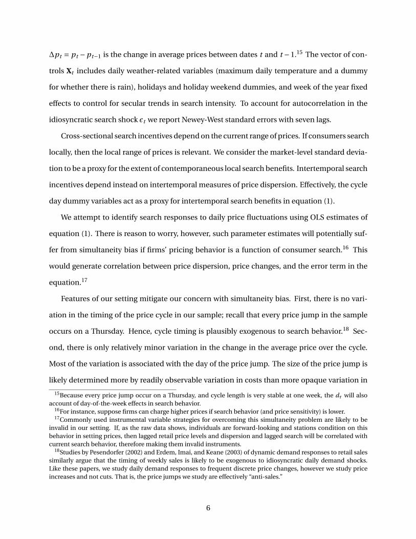
∆pt = pt −pt−1 is the change in average prices between dates t and t −1.15 The vector of con-
trols Xt includes daily weather-related variables (maximum daily temperature and a dummy
for whether there is rain), holidays and holiday weekend dummies, and week of the year fixed
effects to control for secular trends in search intensity. To account for autocorrelation in the
idiosyncratic search shock εt we report Newey-West standard errors with seven lags.
Cross-sectional search incentives depend on the current range of prices. If consumers search
locally, then the local range of prices is relevant. We consider the market-level standard devia-
tion to be a proxy for the extent of contemporaneous local search benefits. Intertemporal search
incentives depend instead on intertemporal measures of price dispersion. Effectively, the cycle
day dummy variables act as a proxy for intertemporal search benefits in equation (1).
We attempt to identify search responses to daily price fluctuations using OLS estimates of
equation (1). There is reason to worry, however, such parameter estimates will potentially suf-
fer from simultaneity bias if firms’ pricing behavior is a function of consumer search.16 This
would generate correlation between price dispersion, price changes, and the error term in the
equation.17
Features of our setting mitigate our concern with simultaneity bias. First, there is no vari-
ation in the timing of the price cycle in our sample; recall that every price jump in the sample
occurs on a Thursday. Hence, cycle timing is plausibly exogenous to search behavior.18 Sec-
ond, there is only relatively minor variation in the change in the average price over the cycle.
Most of the variation is associated with the day of the price jump. The size of the price jump is
likely determined more by readily observable variation in costs than more opaque variation in
15Because every price jump occur on a Thursday, and cycle length is very stable at one week, the dτ will alsoaccount of day-of-the-week effects in search behavior.
16For instance, suppose firms can charge higher prices if search behavior (and price sensitivity) is lower.17Commonly used instrumental variable strategies for overcoming this simultaneity problem are likely to be
invalid in our setting. If, as the raw data shows, individuals are forward-looking and stations condition on thisbehavior in setting prices, then lagged retail price levels and dispersion and lagged search will be correlated withcurrent search behavior, therefore making them invalid instruments.
18Studies by Pesendorfer (2002) and Erdem, Imai, and Keane (2003) of dynamic demand responses to retail salessimilarly argue that the timing of weekly sales is likely to be exogenous to idiosyncratic daily demand shocks.Like these papers, we study daily demand responses to frequent discrete price changes, however we study priceincreases and not cuts. That is, the price jumps we study are effectively “anti-sales.”
6
consumer search.19
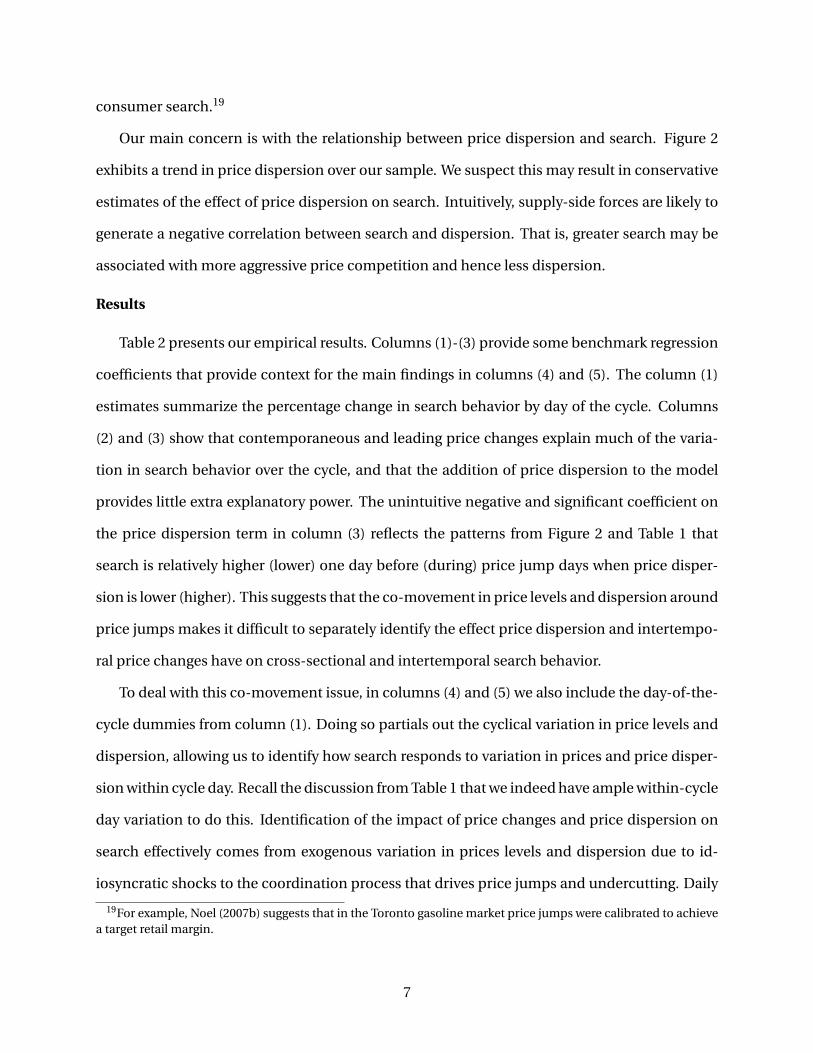
Our main concern is with the relationship between price dispersion and search. Figure 2
exhibits a trend in price dispersion over our sample. We suspect this may result in conservative
estimates of the effect of price dispersion on search. Intuitively, supply-side forces are likely to
generate a negative correlation between search and dispersion. That is, greater search may be
associated with more aggressive price competition and hence less dispersion.
Results
Table 2 presents our empirical results. Columns (1)-(3) provide some benchmark regression
coefficients that provide context for the main findings in columns (4) and (5). The column (1)
estimates summarize the percentage change in search behavior by day of the cycle. Columns
(2) and (3) show that contemporaneous and leading price changes explain much of the varia-
tion in search behavior over the cycle, and that the addition of price dispersion to the model
provides little extra explanatory power. The unintuitive negative and significant coefficient on
the price dispersion term in column (3) reflects the patterns from Figure 2 and Table 1 that
search is relatively higher (lower) one day before (during) price jump days when price disper-
sion is lower (higher). This suggests that the co-movement in price levels and dispersion around
price jumps makes it difficult to separately identify the effect price dispersion and intertempo-
ral price changes have on cross-sectional and intertemporal search behavior.
To deal with this co-movement issue, in columns (4) and (5) we also include the day-of-the-
cycle dummies from column (1). Doing so partials out the cyclical variation in price levels and
dispersion, allowing us to identify how search responds to variation in prices and price disper-
sion within cycle day. Recall the discussion from Table 1 that we indeed have ample within-cycle
day variation to do this. Identification of the impact of price changes and price dispersion on
search effectively comes from exogenous variation in prices levels and dispersion due to id-
iosyncratic shocks to the coordination process that drives price jumps and undercutting. Daily
19For example, Noel (2007b) suggests that in the Toronto gasoline market price jumps were calibrated to achievea target retail margin.
7

wholesale cost shocks, for example, might generate such residual variation in prices and search
within cycle day.
Columns (4) and (5) reveal statistically and economically significant relationships between
search and both price dispersion and price changes. Comparing the column (1) and (4) es-
timates, we see that adding price dispersion to the model has a particularly large impact on
the price jump day coefficient. This is consistent with our discussion of Figure 2: there are
heightened cross-sectional search incentives on price jump days when firms fail to perfectly
coordinate on price jumps, and price dispersion is particularly pronounced.
The column (5) estimates show the search – price dispersion relationship is robust to the
inclusion of price changes in the model. They further show that search rises with larger leading
and contemporaneous price changes. The leading price changes effect is evidence of intertem-
poral search behavior and stockpiling.20 The contemporaneous effects are consistent with pre-
dictions from Lewis (2011) that consumers have reference prices, and that (all else equal) in-
creases in price levels signal there are deals to be found in the market, which results in an
increase in search activity.21 The coefficients on the cycle day dummies also exhibit a trend
increase in search as we approach the cycle minimum, consistent with a stockpiling process in
which a growing body of consumers need to fill up as we approach the trough.
To get a sense of the magnitude of these estimates, a one standard deviation increase in
the price jump of 2 cpl leads to an anticipatory 2% increase in search behavior the day before
the price jump, and a 3.2% increase on the price jump day. Similarly, a one standard deviation
increase in price dispersion on a price jump day of 0.81 cpl leads to a similar 2.4% increase
in search intensity. That is, the effects of price dispersion and intertemporal price changes
on cross sectional and stockpiling effects yield similar contributions to within price jump day
increases in search intensity.22 By comparison, the weekly cycle in search intensity exhibits
20Local media coverage may also play a role. Price rises are highlighted on evening news broadcasts of ChannelSeven, one of the local commercial television stations. In addition, a subset of consumers who have signed up toan email notification service will be alerted to upcoming “price hikes”.
21Within only one year of data for one market, we cannot estimate search models by day of the cycle, given theneed to include week fixed effects in our specifications to control for secular trends in search levels.
22All of the results in this section, both in terms of signs and magnitudes, are robust to the following robustness
8

swings an order of magnitude greater.
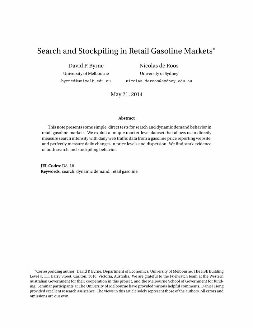
Figure 3 provides further evidence on the relative importance of cross-sectional and in-
tertemporal search. The government provided us with auxiliary data on the aggregate number
of monthly website hits by hour of the day for each for the 14 months in our sample. With these
data, we depict the median, 25th, and 75th percentiles of the distribution of the share of website
hits by hour of the day across the months in the figure. Recalling how the policy works, between
2:30pm and 6am in a given day, consumers can search on the website and receive information
on the distribution of prices today and tomorrow, so both cross sectional and intertemporal
search incentives potentially play a role. Between 6am and 2:30pm there is only information on
today’s prices, implying cross sectional search incentives will dominate.
The large rise in search intensity between 2pm and 3pm, which is exactly when tomorrow’s
prices are posted online, highlights the importance of dynamic incentives for search behavior.23
Between 2pm and 6pm each day, nearly 40% of a typical day’s search occurs. Cross-sectional
search incentives are also quantitatively relevant. Between 6am and 9am each day, during the
morning commute when only information on current prices is available, approximately 14% of
a day’s search occurs.
checks on the specification of equation (1): using Searcht in levels as the dependent variable, using the inter-quartile range as the price dispersion measure, and the inclusion of various other regressors (lagged retail pricechanges up to seven lags, the size of the previous price jump before date t , lags of the dependent variable up toseven lags).
23There are alternative explanations for the peak in search in the afternoon. First, afternoon search is moreefficient: information for two days is available at once, lowering search costs per data point. Second, consumersmay face different time pressures in the morning and afternoon. For example, consumers may be in a rush toget to work in the morning, and find searching for petrol prices an attractive alternative to work activities in theafternoon. We are unable to control for these possibilities.
9

ReferencesBAYE, M. R., J. MORGAN, AND P. SCHOLTEN (2006): “Information, Search, and Price Dispersion,” In Hendershott,
Terry (Eds.), Handbook on Economics and Information.
BROWN, J. R., AND A. GOOLSBEE (2002): “Does the Internet Make Markets More Competitive? Evidence from theLife Insurance Industry,” Journal of Political Economy, 110, 481–507.
BYRNE, D. P., G. W. LESLIE, AND R. WARE (2014): “How do Consumers Respond to Gasoline Price Cycles?,” TheEnergy Journal, forthcoming.
CHANDRA, A., AND M. TAPPATA (2011): “Consumer Search and Dynamic Price Dispersion: An Application to Gaso-line Markets,” Rand Journal of Economics, 42(4), 681–704.
DE LOS SANTOS, B., A. HORTACSU, AND M. R. WILDENBEEST (2012): “Testing Models of Consumer Search UsingData on Web Browsing and Purchasing Behavior,” American Economic Review, 102(6), 2955–2980.
DE ROOS, N., AND H. KATAYAMA (2013): “Gasoline price cycles under discrete time pricing,” Economic Record,89(3), 175–193.
ECKERT, A. (2013): “Empirical Studies of Gasoline Retailing: A Guide to the Literature,” Journal of Economic Sur-veys, 27(1), 140–166.
ERDEM, T., S. IMAI, AND M. P. KEANE (2003): “Brand and Quantity Choice Dynamics Under Price Uncertainty,”Quantitative Marketing and Economics, 1(1), 5–64.
FOROS, O., AND F. STEEN (2013): “Vertical Control and Price Cycles in Gasoline Retailing,” Scandinavian Journalof Economics, 115(3), 640–661.
HENDEL, I., AND A. NEVO (2006a): “Measuring the Implications of Sales and Consumer Inventory Behavior,”Econometrica, 74(6), 1637–1673.
(2006b): “Sales and Consumer Inventory Behavior,” Rand Journal of Economics, 37(3), 543–561.
LEVIN, L., M. S. LEWIS, AND F. A. WOLAK (2012): “High Frequency Evidence on the Demand for Gasoline,” mimeo,Ohio State University.
LEWIS, M. S. (2011): “Asymmetric Price Adjustment and Consumer Search: An Examination of the Retail GasolineMarket,” Journal of Economics and Management Strategy, 20(2), 409–449.
(2012): “Price Leadership and Coordination in Retail Gasoline Markets with Price Cycles,” InternationalJournal of Industrial Organization, 30(4), 342–351.
LEWIS, M. S., AND H. P. MARVEL (2011): “When Do Consumers Search?,” Journal of Industrial Economics, 59(3),457–483.
NOEL, M. D. (2007b): “Edgeworth Price Cycles: Evidence from the Toronto Retail Gasoline Market,” Journal ofIndustrial Economics, 55(1), 69–92.
PELTZMAN, S. (2000): “Prices Rise Faster than They Fall,” Journal of Political Economy, 108, 466–502.
PESENDORFER, M. (2002): “Retail Sales: A Study of Pricing Behavior in Supermarkets,” The Journal of Business,75(1), 33–66.
SEILER, S. (2013): “The Impact of Search Costs on Consumer Behavior: A Dynamic Approach,” Quantitative Mar-keting and Economics, 11(2), 155–203.
10

SORENSEN, A. (2000): “Equilibrium Price Dispersion in Retail Markets for Prescription Drugs,” Journal of PoliticalEconomy, 108(4), 833–850.
WANG, Z. (2009): “(Mixed) Strategies in Oligopoly Pricing: Evidence from Gasoline Price Cycles before and undera Timing Regulation,” Journal of Political Economy, 117(6), 987–1030.
11

Figures and Tables
Figure 1: Fuelwatch Online Price Reports(January 19, 2014)
Home About FuelWatch My FuelWatch Price Search FuelWatch News Fuel Information For Industry
Items per page 20
FuelWatch Quick Search - ResultsProduct: ULP Brands: Any BrandMetro Region: Any Metro Country Region: NoneSuburbs: PERTH (including surrounding suburbs) Date: Today and tomorrow
Refine Search New Search
Best prices available from 6:00am for today and tomorrow
Today Tomorrow Product Brand NameMouse over Name for details
Address Suburb/Town Map
146.7 155.7 ULP United United Mt Lawley 791 Beaufort Street MT LAWLEY
147.7 156.5 ULP United United Northbridge 31 Fitzgerald Street NORTHBRIDGE
153.4 153.4 ULP Gull Gull East Perth Cnr Pier St & Brisbane Sts EAST PERTH
158.9 156.9 ULP Gull Gull First Avenue MtLawley
81 Guildford Rd MT LAWLEY
159.9 157.9 ULP BP BP Connect East Perth Cnr East Parade & BrownStreet
EAST PERTH
159.9 157.9 ULP Caltex Caltex StarMart East Perth 157 Lord St EAST PERTH
159.9 157.9 ULP CaltexWoolworths
Caltex WoolworthsHighgate
Cnr Beaufort St & Bulwer St HIGHGATE
159.9 155.9 ULP Caltex Caltex StarShop Mt Lawley 810 Beaufort Street MT LAWLEY
159.9 158.9 ULP Coles Express Coles Express Highgate 1-5 Guildford Rd MT LAWLEY
159.9 158.9 ULP Coles Express Coles Express Perth 480 William St PERTH
159.9 157.9 ULP Caltex Caltex Wellington Street 141 Wellington Street PERTH
159.9 158.9 ULP Coles Express Coles Express West Perth Cnr Wellington & Thomas Sts WEST PERTH
12 Prices found
The Department of Commerce does not endorse commercial products or services. In order to viewparts of this site it is necessary to enable cookies on your browser. No personal information iseither captured or stored by FuelWatch.This page is copyright © 2011 Department of Commerce .
Home Contact Us Links FAQ Help RSS Sitemap
12

Figure 2: Search, Price Levels, and Price Dispersion
Panel A: Search and Price Levels
5000
1000
015
000
2000
025
000
Dai
ly F
uelw
atch
Web
site
Hits
130
135
140
145
150
155
Aver
age
Ret
ail G
asol
ine
Pric
e (c
pl)
01feb2013 01mar2013 01apr2013 01may2013Date
Retail Price Website Visits
Panel B: Search and Price Dispersion
5000
10000
15000
20000
25000
Daily
Fuelw
atc
h W
ebsite H
its
02
46
8A
vera
ge R
eta
il G
asolin
e P
rice (
cpl)
01feb2013 01mar2013 01apr2013 01may2013Date
Retail Price Website Visits
13

Figure 3: Search Intensity by Hour of the Day(January 19, 2014)
0.0
2.0
4.0
6.0
8.1
De
nsity
12am 2a
m4a
m6a
m8a
m10
am12
pm 2pm
4pm
6pm
8pm
10pm
Hour of the Day
14
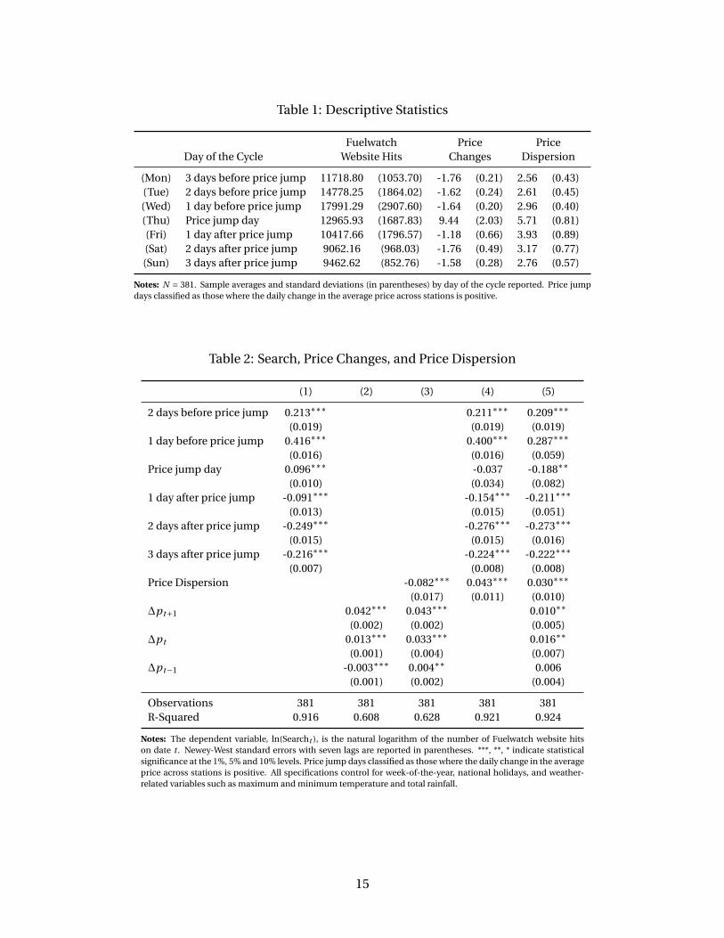
Table 1: Descriptive Statistics
Fuelwatch Price PriceDay of the Cycle Website Hits Changes Dispersion
(Mon) 3 days before price jump 11718.80 (1053.70) -1.76 (0.21) 2.56 (0.43)(Tue) 2 days before price jump 14778.25 (1864.02) -1.62 (0.24) 2.61 (0.45)(Wed) 1 day before price jump 17991.29 (2907.60) -1.64 (0.20) 2.96 (0.40)(Thu) Price jump day 12965.93 (1687.83) 9.44 (2.03) 5.71 (0.81)(Fri) 1 day after price jump 10417.66 (1796.57) -1.18 (0.66) 3.93 (0.89)(Sat) 2 days after price jump 9062.16 (968.03) -1.76 (0.49) 3.17 (0.77)(Sun) 3 days after price jump 9462.62 (852.76) -1.58 (0.28) 2.76 (0.57)
Notes: N = 381. Sample averages and standard deviations (in parentheses) by day of the cycle reported. Price jumpdays classified as those where the daily change in the average price across stations is positive.
Table 2: Search, Price Changes, and Price Dispersion
(1) (2) (3) (4) (5)
2 days before price jump 0.213∗∗∗ 0.211∗∗∗ 0.209∗∗∗(0.019) (0.019) (0.019)
1 day before price jump 0.416∗∗∗ 0.400∗∗∗ 0.287∗∗∗(0.016) (0.016) (0.059)
Price jump day 0.096∗∗∗ -0.037 -0.188∗∗(0.010) (0.034) (0.082)
1 day after price jump -0.091∗∗∗ -0.154∗∗∗ -0.211∗∗∗(0.013) (0.015) (0.051)
2 days after price jump -0.249∗∗∗ -0.276∗∗∗ -0.273∗∗∗(0.015) (0.015) (0.016)
3 days after price jump -0.216∗∗∗ -0.224∗∗∗ -0.222∗∗∗(0.007) (0.008) (0.008)
Price Dispersion -0.082∗∗∗ 0.043∗∗∗ 0.030∗∗∗(0.017) (0.011) (0.010)
∆pt+1 0.042∗∗∗ 0.043∗∗∗ 0.010∗∗(0.002) (0.002) (0.005)
∆pt 0.013∗∗∗ 0.033∗∗∗ 0.016∗∗(0.001) (0.004) (0.007)
∆pt−1 -0.003∗∗∗ 0.004∗∗ 0.006(0.001) (0.002) (0.004)
Observations 381 381 381 381 381R-Squared 0.916 0.608 0.628 0.921 0.924
Notes: The dependent variable, ln(Searcht ), is the natural logarithm of the number of Fuelwatch website hitson date t . Newey-West standard errors with seven lags are reported in parentheses. ***, **, * indicate statisticalsignificance at the 1%, 5% and 10% levels. Price jump days classified as those where the daily change in the averageprice across stations is positive. All specifications control for week-of-the-year, national holidays, and weather-related variables such as maximum and minimum temperature and total rainfall.
15