SE313: Computer Graphics and Visual Programming - …€¦ · Web viewMake sure you understand...

Material for week 6 starts at page 17

SE313: Computer Graphics and Visual Programming

Computer Graphics Notes – Gazihan Alankus, Spring 2012

Computer Graphics

3D computer graphics: geometric modeling of objects in the computer and rendering them

Geometrical model on the computer -> Image on the screen

Define the model in Cartesian coordinates (x, y, z)

You could do the calculations yourself, but graphics packages like OpenGL does this for us.

1


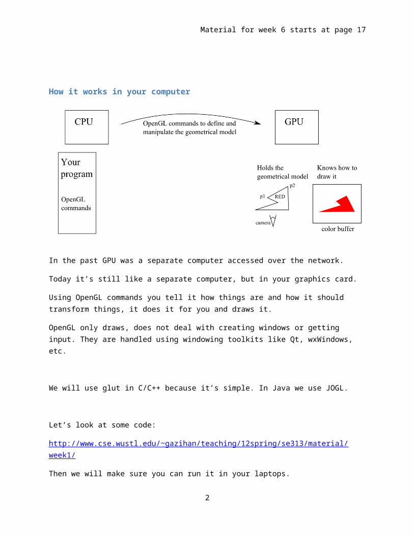
How it works in your computer

In the past GPU was a separate computer accessed over the network.

Today it’s still like a separate computer, but in your graphics card.

Using OpenGL commands you tell it how things are and how it should transform things, it does it for you and draws it.

OpenGL only draws, does not deal with creating windows or getting input. They are handled using windowing toolkits like Qt, wxWindows, etc.

We will use glut in C/C++ because it’s simple. In Java we use JOGL.

Let’s look at some code:

http://www.cse.wustl.edu/~gazihan/teaching/12spring/se313/material/week1/

Then we will make sure you can run it in your laptops.

Note: We learned about glut and OpenGL primitives using slides from week 3. We also learned about different coordinate frames (modeling, world, etc.) Here is an incomplete summary:

2

http://www.cse.wustl.edu/~gazihan/teaching/12spring/se313/material/week1/


Different coordinate frames“Here is the center of the world” –Nasreddin Hoca

You can take your reference point to be anywhere you want, as long as you are consistent. We’ll see that different things have different reference frames.

Modeling coordinatesAn artist creates a model and gives it to you. It inherently has a coordinate frame.

Let’s say the artist creates a house and a tree in two different files. Both files have an origin and coordinate frames. These coordinates of the house and the tree are called modeling coordinates.

World coordinatesThe art assets by themselves are not very useful and we want to create a scene out of them. Therefore, we want to bring them in to a new coordinate frame. This is called world coordinates or scene

3


coordinates.

Above is an empty world with a coordinate frame.

Now we want to place our house and the tree in the world. If we just put the geometric models in the world, here is what it would look like:

4


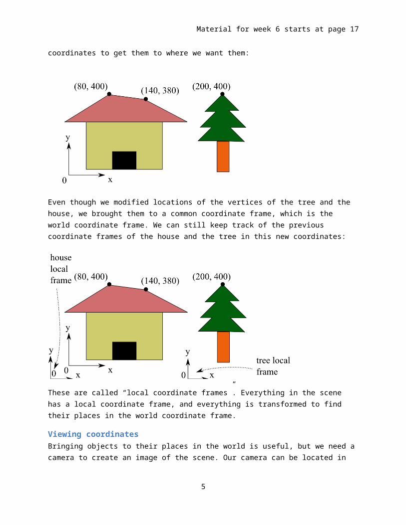
This is not what we want. We want the house to be lower and the tree on the right. We add and subtract to the house’s and the tree’s coordinates to get them to where we want them:

Even though we modified locations of the vertices of the tree and the house, we brought them to a common coordinate frame, which is the world coordinate frame. We can still keep track of the previous coordinate frames of the house and the tree in this new coordinates:

These are called “local coordinate frames”. Everything in the scene has a local coordinate frame, and everything is transformed to find their places in the world coordinate frame.

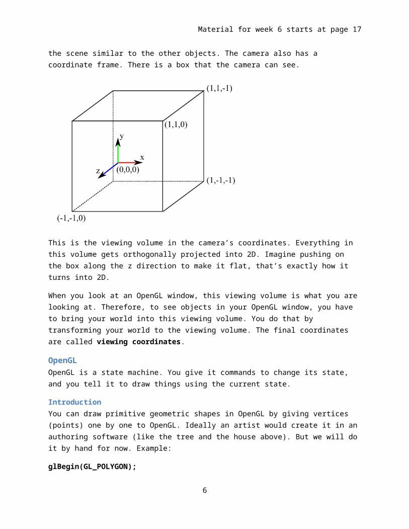
Viewing coordinatesBringing objects to their places in the world is useful, but we need a camera to create an image of the scene. Our camera can be located in the scene similar to the other objects. The camera also has a coordinate frame. There is a box that the camera can see.

5


This is the viewing volume in the camera’s coordinates. Everything in this volume gets orthogonally projected into 2D. Imagine pushing on the box along the z direction to make it flat, that’s exactly how it turns into 2D.

When you look at an OpenGL window, this viewing volume is what you are looking at. Therefore, to see objects in your OpenGL window, you have to bring your world into this viewing volume. You do that by transforming your world to the viewing volume. The final coordinates are called viewing coordinates.

OpenGLOpenGL is a state machine. You give it commands to change its state, and you tell it to draw things using the current state.

IntroductionYou can draw primitive geometric shapes in OpenGL by giving vertices (points) one by one to OpenGL. Ideally an artist would create it in an authoring software (like the tree and the house above). But we will do it by hand for now. Example:

glBegin(GL_POLYGON);

glVertex2f(-0.5, -0.5);

glVertex2f(-0.5, 0.5);

glVertex2f(0.5, 0.5);

glVertex2f(0.5, -0.5);

glEnd();

6


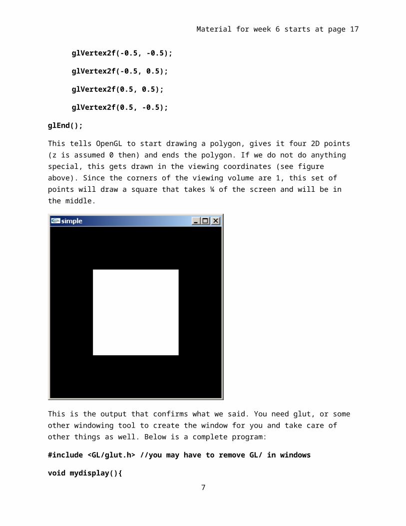
This tells OpenGL to start drawing a polygon, gives it four 2D points (z is assumed 0 then) and ends the polygon. If we do not do anything special, this gets drawn in the viewing coordinates (see figure above). Since the corners of the viewing volume are 1, this set of points will draw a square that takes ¼ of the screen and will be in the middle.

This is the output that confirms what we said. You need glut, or some other windowing tool to create the window for you and take care of other things as well. Below is a complete program:

#include <GL/glut.h> //you may have to remove GL/ in windows

void mydisplay(){

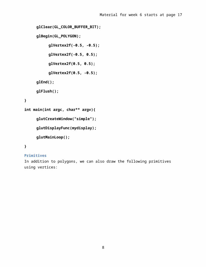
glClear(GL_COLOR_BUFFER_BIT);

glBegin(GL_POLYGON);

glVertex2f(-0.5, -0.5);

glVertex2f(-0.5, 0.5);

glVertex2f(0.5, 0.5);

glVertex2f(0.5, -0.5);

glEnd();

glFlush();

7


}

int main(int argc, char** argv){

glutCreateWindow("simple");

glutDisplayFunc(mydisplay);

glutMainLoop();

}

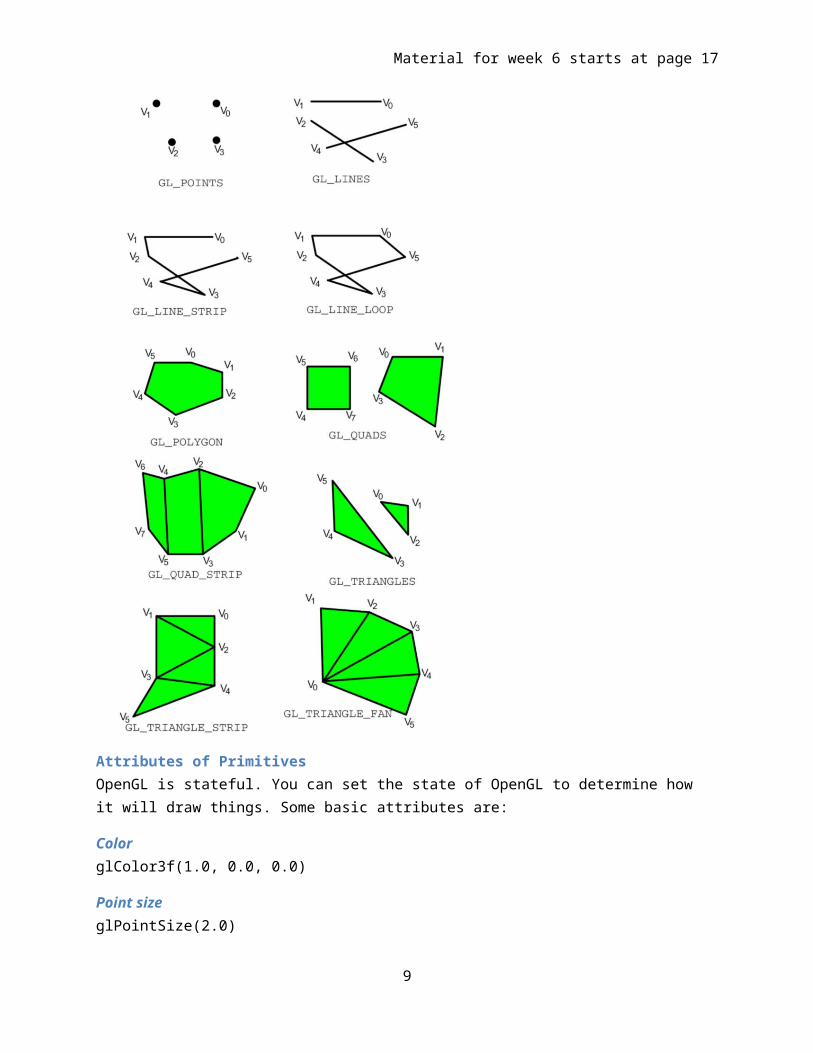
PrimitivesIn addition to polygons, we can also draw the following primitives using vertices:

8


Attributes of PrimitivesOpenGL is stateful. You can set the state of OpenGL to determine how it will draw things. Some basic attributes are:

ColorglColor3f(1.0, 0.0, 0.0)

Point sizeglPointSize(2.0)

9


Line widthglLineWidth(2.0)

Line patternglEnable(GL_LINE_STIPPLE)

glLineStipple(1, 0x1C47)

glDisable(GL_LINE_STIPPLE)

Color blendingglEnable(GL_BLEND);

glDisable(GL_BLEND);

Polygon modesglPolygonMode()

Play with them to see how they change things. Google them and read man pages.

GlutGlut opens the window for you and runs some functions that you give to it. These are called “callback functions” because glut calls them back when it needs to.

glutDisplayFunc(renderScene);

glutReshapeFunc(changeSize);

glutIdleFunc(renderScene);

glutKeyboardFunc(processNormalKeys);

glutSpecialFunc(processSpecialKeys);

You create the functions that we gave as arguments (renderScene, changeSize, etc.). Glut calls them when necessary. Glut takes care of keyboard input, too.

There is a great tutorial here

Some important conventions to keep in mind about Glut: Never call the callback functions (renderScene etc.) yourself. Always let Glut call them. Only set the callback functions in the main function. For example, do not call

glutDisplayFunc(someOtherRenderScene); to change what’s being rendered. Instead, use variables to keep state, and let the renderScene function act differently with respect to those variables.

Animation with glutHere is why we observe animation:

10

http://www.lighthouse3d.com/tutorials/glut-tutorial/


Glut calls your renderScene function many times a secondo This is because you set up a timer with glutTimerFunc(10, updateScene, 0); and in it,

force glut to repaint the screen using glutPostRedisplay() Your renderScene function acts differently in time

o This is because you change the program state using variables

You need to have some variables that define the current state of the animation, make the renderScene function use those variables to draw the scene, and change those variables in updateScene so that renderScene draws something different the next time it is called.

When you animate and see flickering on screen, it may be because you did not open your window in double-buffered mode: glutInitDisplayMode(GLUT_DEPTH | GLUT_DOUBLE | GLUT_RGBA);

With double buffering, the frame you see is not the one that OpenGL is currently drawing. This way, we never see incomplete frames.

Drawing in three dimensionsUp till now we drew OpenGL primitives in two dimensions and we used calls like glVertex2d(0.5, 1.0); to specify points using their x and y coordinates. In three dimensions, we also have the z coordinate, and specify vertices this way: glVertex3d(0.5, 1.0, 0.2);

In fact, when you specify a two dimensional vertex, it is equivalent to specifying one with the z coordinate equal to zero. Therefore, the following are equivalent:

glVertex2d(0.5, 1.0);

glVertex3d(0.5, 1.0, 0.0);

We can use any 3D point to specify the vertices for our OpenGL primitives. By locating the camera in an arbitrary location in the space (we will learn later) we can take a virtual picture of the scene.

Orthographic vs. Perspective ProjectionTaking virtual pictures is achieved using projection of 3D points to a 2D plane, as we talked about in class before. There are two methods: orthogonal projection and perspective projection.

11


[Images are borrowed from http://db-in.com]

By default the projection is orthographic. In orthographic projection when things move away they do not get smaller. In perspective projection, they become smaller like it is in the real world. Both have their uses.

In orthographic projection, we simply move and scale the world to fit them in our viewing half cube, and project it to 2D.

12

http://db-in.com/


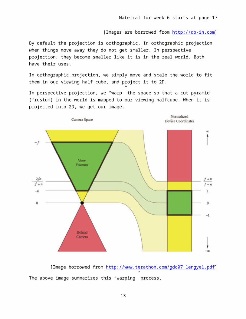
In perspective projection, we “warp” the space so that a cut pyramid (frustum) in the world is mapped to our viewing halfcube. When it is projected into 2D, we get our image.

[Image borrowed from http://www.terathon.com/gdc07_lengyel.pdf]

The above image summarizes this “warping” process.

We can set the parameters of the orthographic projection using glOrtho(left, right, bottom, top, near, far), or if we don’t care about the z axis, gluOrtho2D(left, right, bottom, top). This is equivalent to calling glOrtho with -1 and 1 for near and far values. OpenGL uses left, right, bottom, top, near, far in world coordinates to define a rectangular volume to be visible. The camera is directed towards the negative z axis.

We can set a perspective projection using glFrustum(left, right, bottom, top, near, far) or gluPerspective(fovy angle, aspect ratio, neardistance, fardistance). In both of them, the eye is located at the origin, there is a near plane and a small rectangle on it that maps to the screen, and a far plane with a larger rectangle. These three are on a pyramid. The following image helps explain this better:

13

http://www.terathon.com/gdc07_lengyel.pdf


gluPerspective is easier to use and should be preferred.

gluPerspective(fovy angle, aspect ratio, neardistance, fardistance).

Fovy angle is the angle between the top and the bottom of the pyramid. Aspect ratio is the width/height of the rectangle. Neardistance is the distance of the near plane to the eye, where we start seeing things. Far distance is the distance to the far plane that we don’t see beyond. After this, we are still looking towards the –z axis.

Therefore, if we start with an identity matrix in our projection matrix, and call

gluPerspective(90, 1.0, 0.1, 100.0)

14


Then what we have at the z=-1 plane stays the same, while everything else scales:

However, it is better to set a fov angle that matches the approximate distance of your eye to the screen and the size of the screen. 40 can be a good approximation.

Setting up projectionProjection is implemented something called “the perspective matrix”. We will learn about the different types of matrices in OpenGL later.

You usually set the projection matrix once and don’t touch it afterwards:

void init() {

glMatrixMode(GL_PROJECTION);

glLoadIdentity();

gluPerspective(40, 1.0, 0.1, 100.0);

}

or

void init() {

glMatrixMode(GL_PROJECTION);

glLoadIdentity();

gluOrtho2D(-100.0, 100.0, -100.0, 100.0);

15


}

We will see how to move and orient the camera later.

16


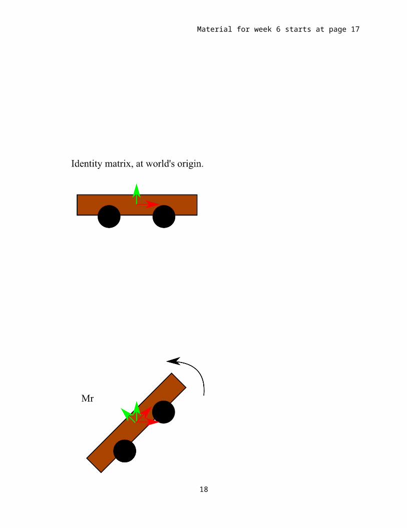
Combining TransformationsNote that matrix multiplication is not commutative. That is, M1.M2 is usually not equal to M2.M1. This is true if any of the matrices do any rotation. Let’s say Mr is a rotation matrix and Mt is a translation matrix. Mr.Mt and Mt.Mr transform the cart differently. Let’s first investigate what it means to combine transformations this way.

If we transform our cart with Mr.Mt, we can think of it two ways:

(1) we first rotate the cart (Mr), and then translate it in the rotated coordinate frame (Mr.Mt) (going inwards),

(2) we first translate the cart (Mt), and rotate the whole world around it (Mr.Mt) (going outwards).

While you are writing OpenGL code, you usually think of it as the first one. However, when dealing with the camera, you may want to think of it as the second way because the viewing matrix always goes first. Let’s assume that Mr rotates 45 degrees counter-clockwise, and Mt moves along the positive X axis and let’s see (1) and (2) in examples. First let’s see what these transformations do by themselves:

17


18


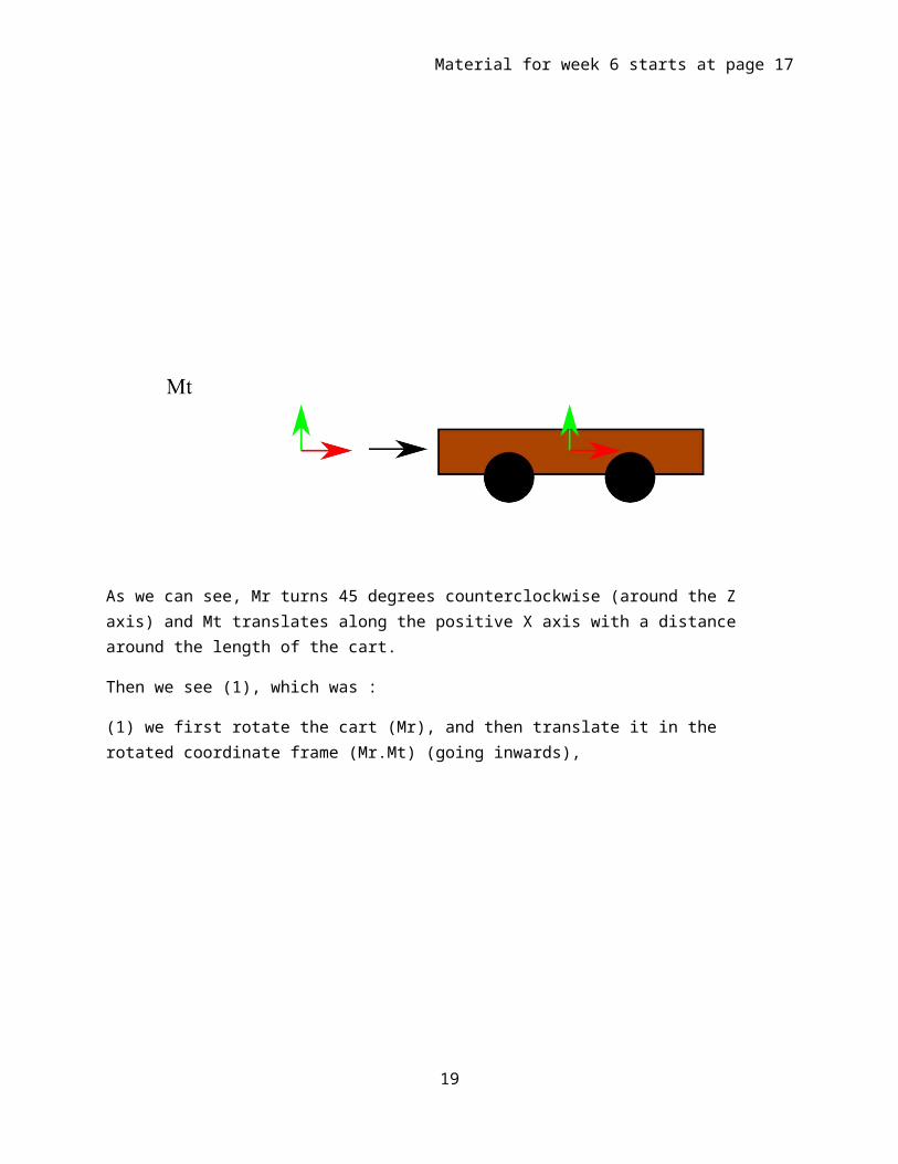
As we can see, Mr turns 45 degrees counterclockwise (around the Z axis) and Mt translates along the positive X axis with a distance around the length of the cart.

Then we see (1), which was :

(1) we first rotate the cart (Mr), and then translate it in the rotated coordinate frame (Mr.Mt) (going inwards),

19


20


As you can see, since Mt was multiplied on the right, it is an “inner” transformation. Therefore the cart is transformed in the local coordinates. Since Mt is supposed to move the cart along the X axis, it moves it in the local X axis, which is 45 degrees turned with the cart.

Now let’s see the second case (2), which was:

(2) we first translate the cart (Mt), and rotate the whole world around it (Mr.Mt) (going outwards).

21


22


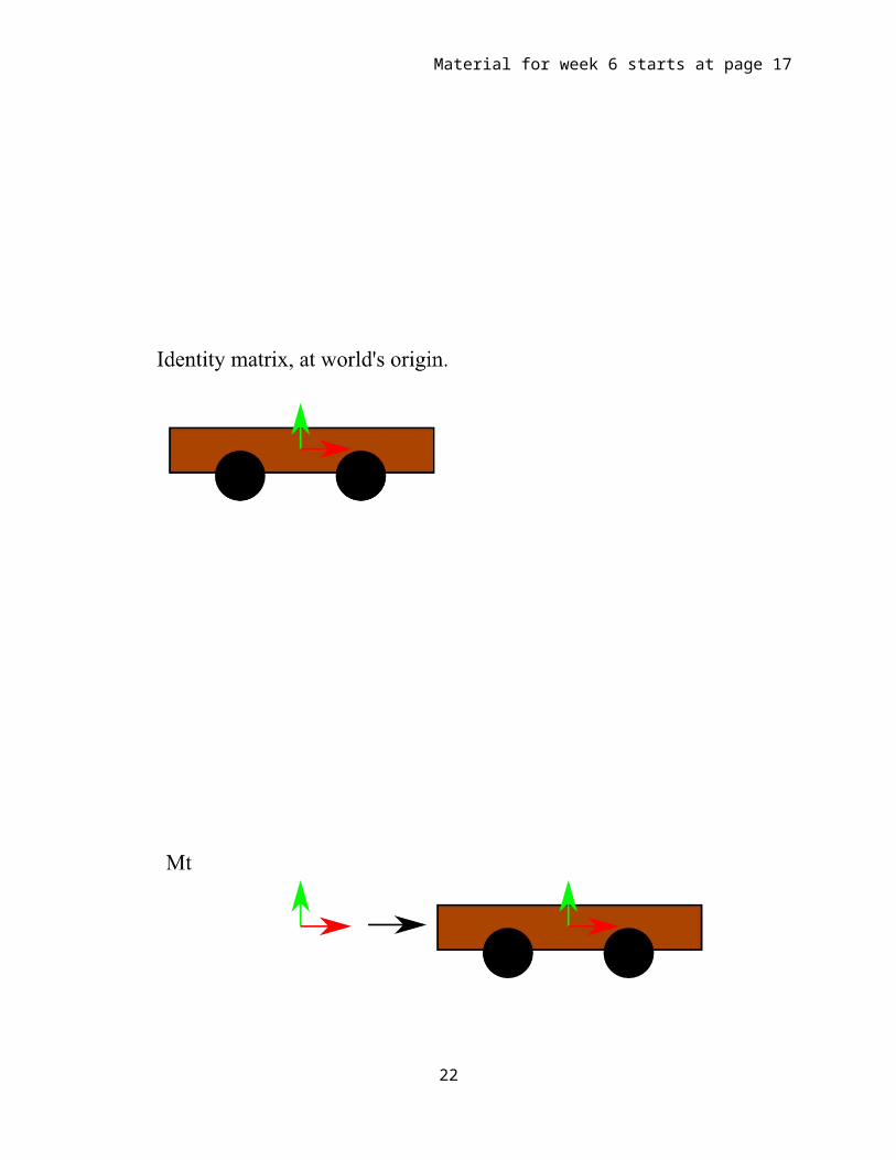
As you can see, since Mr was multiplied on the left, it is an “outer” transformation. Therefore the cart is transformed in the word coordinates, around the world’s origin. Since Mr is supposed to rotate the cart 45 degrees counterclockwise, it rotated the whole world, including the translation of the cart.

This was Mr.Mt. Let’s see what Mt.Mr does. First going from world to local like (1):

23


24


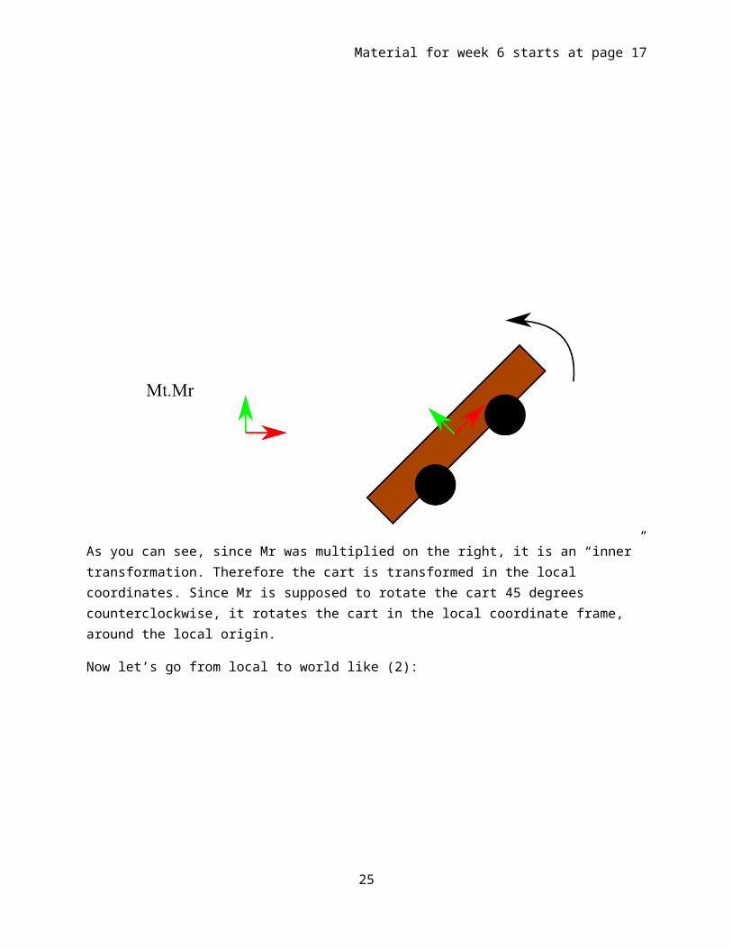
As you can see, since Mr was multiplied on the right, it is an “inner” transformation. Therefore the cart is transformed in the local coordinates. Since Mr is supposed to rotate the cart 45 degrees counterclockwise, it rotates the cart in the local coordinate frame, around the local origin.

Now let’s go from local to world like (2):

25


26


As you can see, since Mt was multiplied on the left, it is an “outer” transformation. Therefore the cart is transformed in the word coordinates, along the world’s x axis. Since Mt is supposed to move the cart along the X axis, it moves it in the world X axis, which is not turned.

Note how Mr.Mt and Mt.Mr are different.

Hopefully, this makes clear the ordering of matrices and what we mean by “local coordinates” and “world coordinates”.

Now that we know how to combine transformations, we can think about how we can set up the camera matrix such that the camera rotates around the object like the earlier figures with the iPhone picture.

Note that in that transformation, the world is first moved away from the camera’s origin, and then rotated in a local coordinate frame. Therefore our camera matrix becomes Mv=Mt.Mr.

Our program can keep track of two variables: cameraDistance and cameraAngle. Then in the locateCamera() function, it can use them as:

void locateCamera() {

glMatrixMode(GL_MODELVIEW);

glLoadIdentity();

27


glTranslatef(0.f, 0.f, -cameraDistance);

glRotatef(cameraAngle, 0.f, 0.f, 0.f); //correct this

//as an exercise please :)

}

This way we load the camera matrix before multiplying it with the model matrices.

Intuitive Understanding of TransformationsPreviously we have seen how transformations work and how they are combined. Here we will see more concrete and easy-to-visualize examples. This will help us have a more intuitive understanding of transformations, how they work and what it means to combine them in different ways. Since transformations were abstract entities, it may have been difficult to understand. Now we will use concrete physical entities that represent transformations and will use them to understand transformations better.

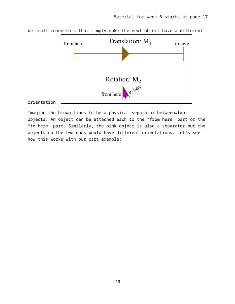
Let us imagine transformations to be physical connectors between objects in the space. You can imagine translations to be straight connectors with both ends having the same orientation and rotations to be small connectors that simply make the next object have a different orientation.

Imagine the brown lines to be a physical separator between two objects. An object can be attached each to the “from here” part or the “to here” part. Similarly, the pink object is also a separator but the objects on the two ends would have different orientations. Let’s see how this works with our cart example:

28


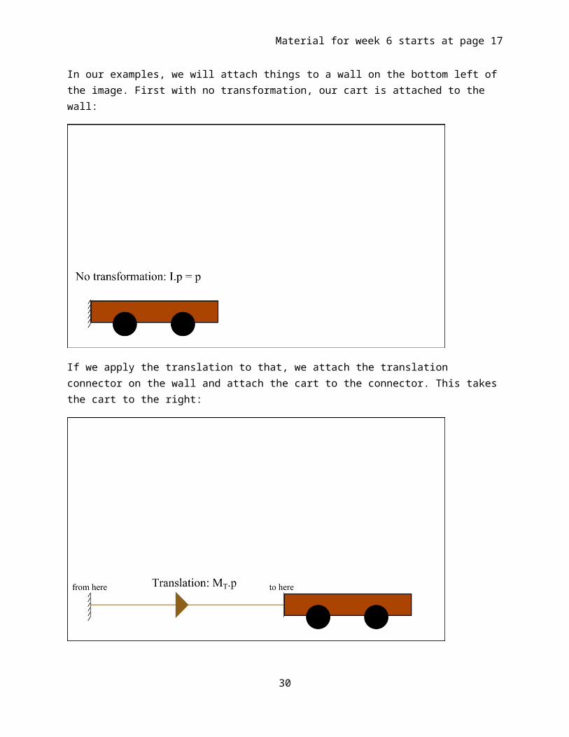
In our examples, we will attach things to a wall on the bottom left of the image. First with no transformation, our cart is attached to the wall:

If we apply the translation to that, we attach the translation connector on the wall and attach the cart to the connector. This takes the cart to the right:

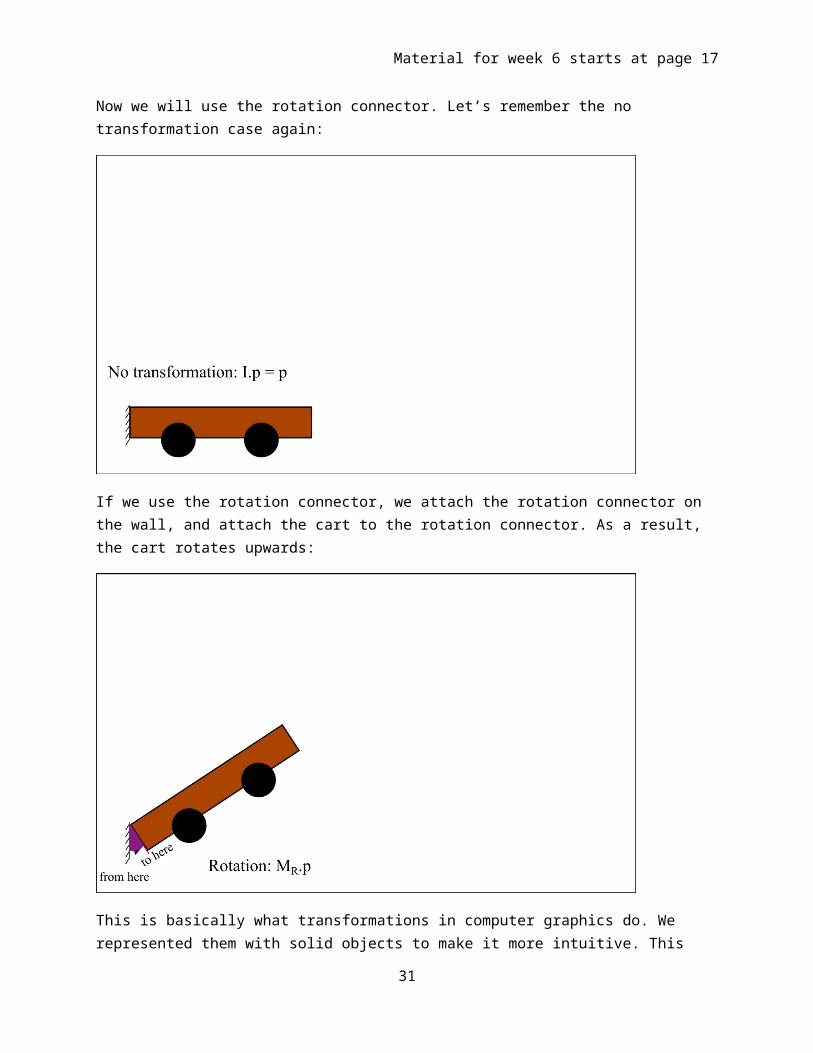
Now we will use the rotation connector. Let’s remember the no transformation case again:

29


If we use the rotation connector, we attach the rotation connector on the wall, and attach the cart to the rotation connector. As a result, the cart rotates upwards:

This is basically what transformations in computer graphics do. We represented them with solid objects to make it more intuitive. This representation especially makes combining transformations more intuitive. Let’s see a basic example:

We start with the empty wall, which is no transformation:

30


Then we add a rotation to it:

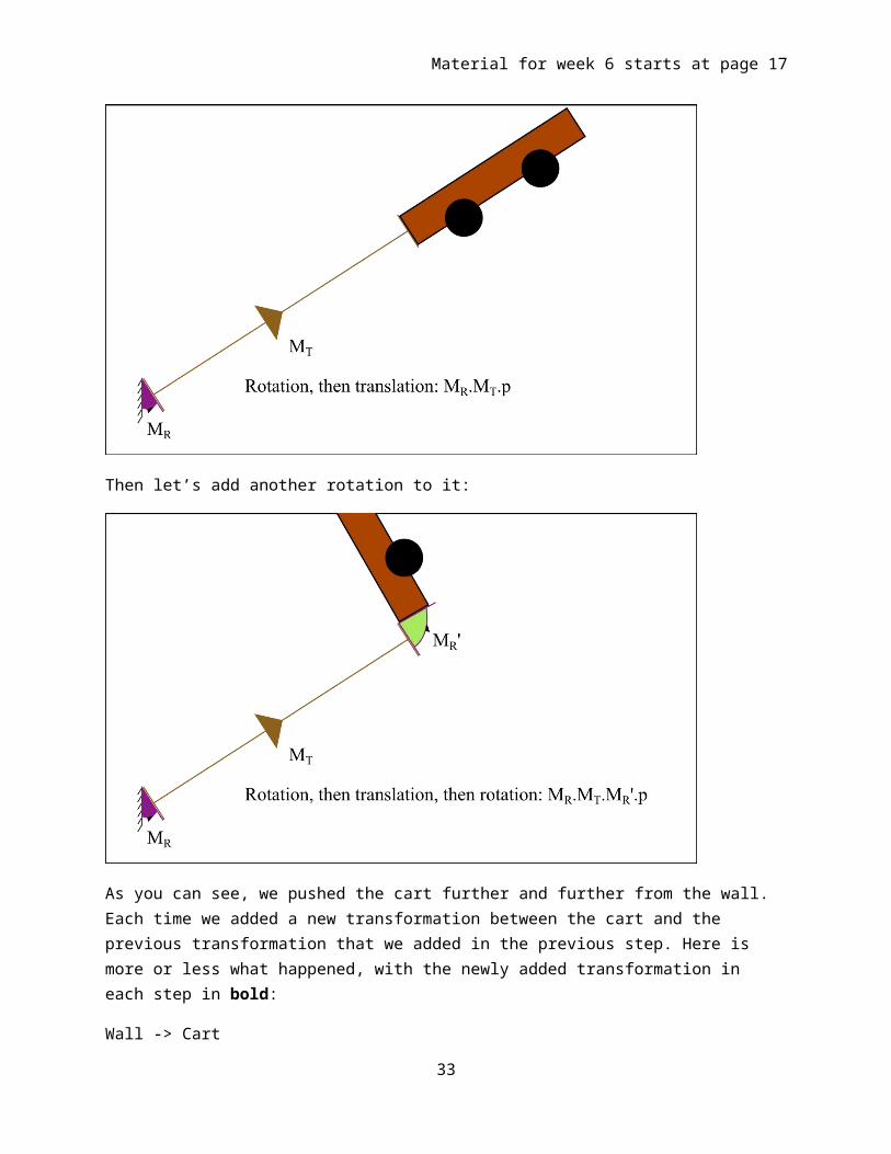
Then we add a translation to it:

31


Then let’s add another rotation to it:

As you can see, we pushed the cart further and further from the wall. Each time we added a new transformation between the cart and the previous transformation that we added in the previous step. Here is more or less what happened, with the newly added transformation in each step in bold:

Wall -> Cart

Wall -> MR -> Cart

32


Wall -> MR -> MT -> Cart

Wall -> MR -> MT -> MR’ -> Cart

As you can see, we always added the transformation right before the cart and after the previously added one. If you follow the transformation matrices in the pictures, here is how it evolved:

p

MR.p

MR.MT.p

MR.MT.MR’.p

As you can see, similarly the newly added matrix was always before p (a point of the cart) and the previously added transformation.

This is what we meant when we said “inner” transformations. As we keep adding transformations like that, those transformations are applied to the end of the transformed chain, which is an “inner” attachment place, not the “world” wall that we had down below on the left.

You can think of this in terms of world coordinates and local coordinates. The wall on bottom left is the world, or the origin of the world coordinates. As we attach transformations, what we attach after those transformations are attached to a “local” wall, that is the end of the transformation piece. That is local coordinates.

By adding transformations at the end and right before the card, we applied transformations in the “cart’s local coordinates” or “local transformations”. Because that was where the cart was, and instead we attached a transformation there.

We could also attach transformations in the “world coordinates” or apply “world transformations”. Since the world is the wall, this would mean that we attach newly added transformations between the wall and whatever is attached to the wall. Let’s see the same example by adding world transformations each time.

Again, we start with our cart on the wall:

33


Then, let’s add the green rotation between the cart and the wall:

Note that even though the transformation that we used was different, this step was exactly the same as our previous example. This is because when there was no transformation, the cart’s local coordinates were equal to the world coordinates. This made world and local transformations be the same thing. If you do not understand this now, come back here later after you saw everything.

Anyway, let’s add a translation in the world coordinates:

34


Since we wanted to transform the cart in world coordinates, we inserted our translation next to the wall (between wall and green rotation). If we wanted to transform the cart in local coordinates, we would insert our translation next to the cart (between cart and green rotation). Understand that the two move the cart differently (local would move the cart upwards, make sure you understand why).

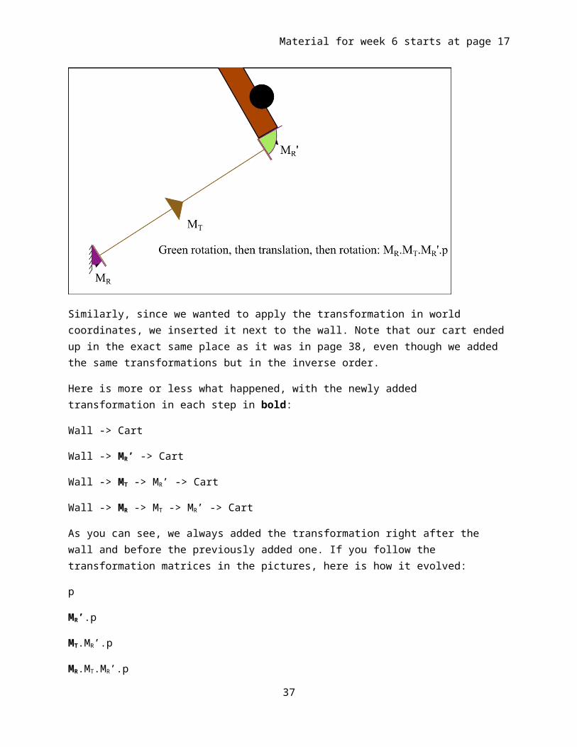
OK, let’s apply one more transformation in world coordinates. This time, let’s add our purple rotation in world coordinates:

35


Similarly, since we wanted to apply the transformation in world coordinates, we inserted it next to the wall. Note that our cart ended up in the exact same place as it was in page 38, even though we added the same transformations but in the inverse order.

Here is more or less what happened, with the newly added transformation in each step in bold:

Wall -> Cart

Wall -> MR’ -> Cart

Wall -> MT -> MR’ -> Cart

Wall -> MR -> MT -> MR’ -> Cart

As you can see, we always added the transformation right after the wall and before the previously added one. If you follow the transformation matrices in the pictures, here is how it evolved:

p

MR’.p

MT.MR’.p

MR.MT.MR’.p

As you can see, similarly the newly added matrix was always before everything else. This is what we meant when we said “outer” transformations. As we keep adding transformations like that, the newly added transformations transformed everything that came after them, because we inserted them before the wall, where everything was attached to.

This is what we meant by “outer” transformations. By transforming everything that exists in the scene, it basically transformed that subspace from “outside”.

You can think of this in terms of world coordinates and local coordinates. The wall on bottom left is the world, or the origin of the world coordinates. The transformations that we attached to the world are world transformations that transform everything else, because where we add the transformation is where the world is.

Note however that even though the matrix multiplications were the same in the two examples, when we talked about them, we listed the transformations in the reverse order:

1. “Rotation, then translation, then green rotation” 2. ”Green rotation, then translation, then rotation”

Because in the first one we assumed that we were talking about the “outside to inside” or “world-to-local” order. In the second one, we assumed that we were talking about the “inside to outside” or “local-to-world” order.

36


Exercise: Using the same MR, MT and MR’, similarly draw these operations in the asked order:

In local-to-world order:o MR, then MT, then MR’o MT, MR’, then MR

In outside to inside order:o MR’, MT, MR

o MT, MR’, then MR

Make sure you understand both directions of thinking about combining transformations. Make sure you understand that the mathematics is the same in each direction, but we are simply trying to make sense of the order of operations in two different ways.

OpenGL and Combining TransformationsIn OpenGL, you give successive commands that postmultiply the current matrix. That is, if the current matrix is M, and we call glRotate(), the current value of the matrix becomes M.MR. As you recall, this is the outer-to-inner or world-to-local ordering. As you keep postmultiplying, you go more and more inside your model. Therefore, as you are writing OpenGL code, you always think of the ordering as world-to-local. The earlier matrix operations transform everything else that come after in code.

The matrix stackNote that in OpenGL the only matrix operations you can do with the current matrix are:

1. glGet*: read the current matrix2. glLoad*: set the current matrix to be a specific matrix3. glMult, glRotate, glTranslate, etc: postmultiply the current matrix with a new matrix

(Mcurrent=Mcurrent.Mnew)

Sometimes, you want to remember the value of the current matrix before you change it to something else (we will see why we would want that soon below). While you could do glGet and save it to somewhere and then do glLoad later, glGet is a very inefficient OpenGL command as it stalls the GPU’s pipeline to read the current value of the matrix. Instead, we can tell the GPU to remember the current matrix for later use. We do this by pushing the matrix to the matrix stack with glPushMatrix() and popping it out later with glPopMatrix(). This way the matrix does not have to leave the GPU, which does not cause inefficiency. Let’s see how this works:

37

Currentmatrix

push change pop


When we want to remember the value of the current matrix later, we push it to the matrix stack. After that, we can change the current matrix freely, postmultiply it, etc. Later, when we want to go back to that old value, we pop it from the top of the stack. Note that you can pop only once for every push. For every push there should be one pop, so that your program functions correctly.

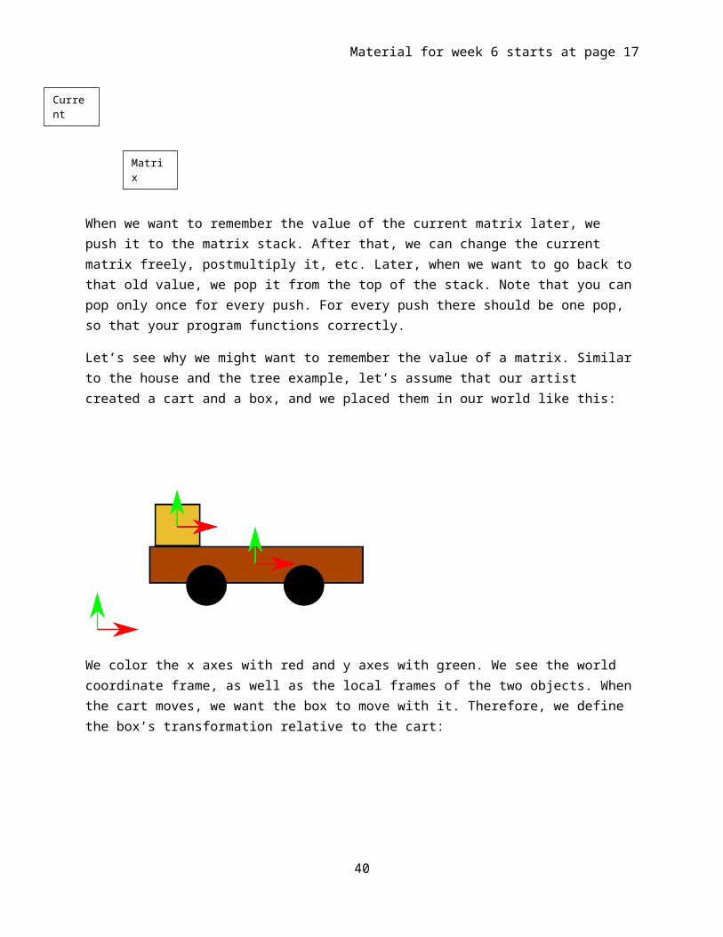
Let’s see why we might want to remember the value of a matrix. Similar to the house and the tree example, let’s assume that our artist created a cart and a box, and we placed them in our world like this:

We color the x axes with red and y axes with green. We see the world coordinate frame, as well as the local frames of the two objects. When the cart moves, we want the box to move with it. Therefore, we define the box’s transformation relative to the cart:

38

Matrixstack


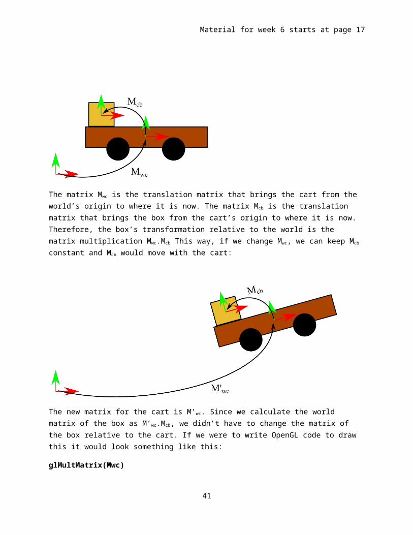
The matrix Mwc is the translation matrix that brings the cart from the world’s origin to where it is now. The matrix Mcb is the translation matrix that brings the box from the cart’s origin to where it is now. Therefore, the box’s transformation relative to the world is the matrix multiplication Mwc.Mcb This way, if we change Mwc, we can keep Mcb constant and Mcb would move with the cart:

The new matrix for the cart is M’wc. Since we calculate the world matrix of the box as M’wc.Mcb, we didn’t have to change the matrix of the box relative to the cart. If we were to write OpenGL code to draw this it would look something like this:

glMultMatrix(Mwc)

drawTheCart()

glMultMatrix(Mcb)

drawTheBox()

Note that instead of glMultMatrix() we usually use a series of glTranslate() and glRotate() calls in actual programs.

As you can see, we are multiplying the current matrix as we go along. If we assume that initially the current matrix was identity, here is the current value of the matrix as we go along:

glMultMatrix(Mwc) //current value of the matrix became Mwc

drawTheCart() //the cart is drawn as Mwc.p

glMultMatrix(Mcb) //current value of the matrix became Mwc.Mcb

drawTheBox() //the box is drawn as Mwc.Mcb.p

This is great. What if we also had a seat on the cart?

39


Everything else is the same, and the seat’s matrix is M’wc.Mcs, that is, the cart’s matrix relative to the world, multiplied by the seat’s matrix relative to the cart. Let’s see how we could implement that in OpenGL:





glMultMatrix(Mcs) //current value of the matrix became Mwc.Mcb.Mcs

drawTheSeat() //the seat is drawn as Mwc.Mcb.Mcs.p

//but it should be Mwc.Mcs.p :(

As you can see, we have a problem. Since the current matrix is M’wc.Mcb, if we multiply it by Mcs, we get M’wc.Mcb.Mcs. However, as we said above, we need it to be M’wc.Mcs for the seat. If only we could “undo” the glMultMatrix(Mcb) step, everything would be fine. Then, the current matrix would go back to being M’wc, and glMultMatrix(Mcs) would make it M’wc.Mcs like we needed. This “undo” mechanism that we need is exactly why we need the matrix stack. Here is how we would fix this code:



glPushMatrix() //I know I’ll need this matrix later



40


glPopMatrix() //current value of the matrix became Mwc again :)

glMultMatrix(Mcs) //current value of the matrix became Mwc.Mcs :)

drawTheSeat() //the seat is drawn as Mwc.Mcs.p :)

As you see, we used glPushMatrix() to store the current matrix on top of the matrix stack, and later retrieved it back using glPopMatrix().

If we draw the relationship between our cart, box and the seat conceptually,

This tree (or more accurately Directed Acyclic Graph) structure is called a scene graph. Scene graphs indicate the parent/child relationships of objects in the scene. They are rendered using a depth-first traversal, with a glPushMatrix() every time we go down a level and a glPopMatrix() every time we go up. This way we can have scene graphs with arbitrary structures. When you are drawing more than one object in a scene, try to think of it like a scene graph, even if you do not represent your data like a graph.

41

SE313: Computer Graphics and Visual Programming - …€¦ · Web viewMake sure you understand...

Documents

Transcript of SE313: Computer Graphics and Visual Programming - …€¦ · Web viewMake sure you understand...