Unbiased Estimation with Square Root Convergence for SDE Models
description
Stochastic Differential Equations
with Applications
December 4, 2012

2

Contents
1 Stochastic Differential Equations 7
1.1 Introduction . . . . . . . . . . . . . . . . . . . . . . . . . . . . . . . . . . . . . . . . . . 7
1.1.1 Meaning of Stochastic Differential Equations . . . . . . . . . . . . . . . . . . . 8
1.2 Some applications of SDEs . . . . . . . . . . . . . . . . . . . . . . . . . . . . . . . . . 10
1.2.1 Asset prices . . . . . . . . . . . . . . . . . . . . . . . . . . . . . . . . . . . . . . 10
1.2.2 Population modelling . . . . . . . . . . . . . . . . . . . . . . . . . . . . . . . . 10
1.2.3 Multi-species models . . . . . . . . . . . . . . . . . . . . . . . . . . . . . . . . . 11
2 Continuous Random Variables 13
2.1 The probability density function . . . . . . . . . . . . . . . . . . . . . . . . . . . . . . 13
2.1.1 Change of independent deviates . . . . . . . . . . . . . . . . . . . . . . . . . . . 13
2.1.2 Moments of a distribution . . . . . . . . . . . . . . . . . . . . . . . . . . . . . . 13
2.2 Ubiquitous probability density functions in continuous finance . . . . . . . . . . . . . . 14
2.2.1 Normal distribution . . . . . . . . . . . . . . . . . . . . . . . . . . . . . . . . . 14
2.2.2 Log-normal distribution . . . . . . . . . . . . . . . . . . . . . . . . . . . . . . . 14
2.2.3 Gamma distribution . . . . . . . . . . . . . . . . . . . . . . . . . . . . . . . . . 14
2.3 Limit Theorems . . . . . . . . . . . . . . . . . . . . . . . . . . . . . . . . . . . . . . . . 15
2.3.1 The central limit results . . . . . . . . . . . . . . . . . . . . . . . . . . . . . . . 17
2.4 The Wiener process . . . . . . . . . . . . . . . . . . . . . . . . . . . . . . . . . . . . . 17
2.4.1 Covariance . . . . . . . . . . . . . . . . . . . . . . . . . . . . . . . . . . . . . . 18
2.4.2 Derivative of a Wiener process . . . . . . . . . . . . . . . . . . . . . . . . . . . 18
2.4.3 Definitions . . . . . . . . . . . . . . . . . . . . . . . . . . . . . . . . . . . . . . 18
3 Review of Integration 21
3
4 CONTENTS
3.1 Bounded Variation . . . . . . . . . . . . . . . . . . . . . . . . . . . . . . . . . . . . . . 21
3.2 Riemann integration . . . . . . . . . . . . . . . . . . . . . . . . . . . . . . . . . . . . . 23
3.3 Riemann-Stieltjes integration . . . . . . . . . . . . . . . . . . . . . . . . . . . . . . . . 24
3.4 Stochastic integration of deterministic functions . . . . . . . . . . . . . . . . . . . . . . 25
4 The Ito and Stratonovich Integrals 27
4.1 A simple stochastic differential equation . . . . . . . . . . . . . . . . . . . . . . . . . . 27
4.1.1 Motivation for Ito integral . . . . . . . . . . . . . . . . . . . . . . . . . . . . . . 28
4.2 Stochastic integrals . . . . . . . . . . . . . . . . . . . . . . . . . . . . . . . . . . . . . . 29
4.3 The Ito integral . . . . . . . . . . . . . . . . . . . . . . . . . . . . . . . . . . . . . . . . 31
4.3.1 Application . . . . . . . . . . . . . . . . . . . . . . . . . . . . . . . . . . . . . . 33
4.4 The Stratonovich integral . . . . . . . . . . . . . . . . . . . . . . . . . . . . . . . . . . 33
4.4.1 Relationship between the Ito and Stratonovich integrals . . . . . . . . . . . . . 35
4.4.2 Stratonovich integration conforms to the classical rules of integration . . . . . . 37
4.5 Stratonovich representation on an SDE . . . . . . . . . . . . . . . . . . . . . . . . . . . 38
5 Differentiation of functions of stochastic variables 41
5.1 Ito’s Lemma . . . . . . . . . . . . . . . . . . . . . . . . . . . . . . . . . . . . . . . . . . 41
5.1.1 Ito’s lemma in multi-dimensions . . . . . . . . . . . . . . . . . . . . . . . . . . 44
5.1.2 Ito’s lemma for products . . . . . . . . . . . . . . . . . . . . . . . . . . . . . . . 45
5.2 Further examples of SDEs . . . . . . . . . . . . . . . . . . . . . . . . . . . . . . . . . . 45
5.2.1 Multi-dimensional Ornstein Uhlenbeck equation . . . . . . . . . . . . . . . . . . 45
5.2.2 Logistic equation . . . . . . . . . . . . . . . . . . . . . . . . . . . . . . . . . . . 46
5.2.3 Square-root process . . . . . . . . . . . . . . . . . . . . . . . . . . . . . . . . . 47
5.2.4 Constant Elasticity of Variance Model . . . . . . . . . . . . . . . . . . . . . . . 48
5.2.5 SABR Model . . . . . . . . . . . . . . . . . . . . . . . . . . . . . . . . . . . . . 48
5.3 Heston’s Model . . . . . . . . . . . . . . . . . . . . . . . . . . . . . . . . . . . . . . . . 49
5.4 Girsanov’s lemma . . . . . . . . . . . . . . . . . . . . . . . . . . . . . . . . . . . . . . . 49
5.4.1 Change of measure for a Wiener process . . . . . . . . . . . . . . . . . . . . . . 51
5.4.2 Girsanov theorem . . . . . . . . . . . . . . . . . . . . . . . . . . . . . . . . . . 52
6 The Chapman Kolmogorov Equation 55
CONTENTS 5
6.1 Introduction . . . . . . . . . . . . . . . . . . . . . . . . . . . . . . . . . . . . . . . . . . 55
6.1.1 Markov process . . . . . . . . . . . . . . . . . . . . . . . . . . . . . . . . . . . . 56
6.2 Chapman-Kolmogorov equation . . . . . . . . . . . . . . . . . . . . . . . . . . . . . . . 57
6.2.1 Path continuity . . . . . . . . . . . . . . . . . . . . . . . . . . . . . . . . . . . . 57
6.2.2 Drift and diffusion . . . . . . . . . . . . . . . . . . . . . . . . . . . . . . . . . . 59
6.2.3 Drift and diffusion of an SDE . . . . . . . . . . . . . . . . . . . . . . . . . . . . 60
6.3 Formal derivation of the Forward Kolmogorov Equation . . . . . . . . . . . . . . . . . 61
6.3.1 Intuitive derivation of the Forward Kolmogorov Equation . . . . . . . . . . . . 66
6.3.2 The Backward Kolmogorov equation . . . . . . . . . . . . . . . . . . . . . . . . 67
6.4 Alternative view of the forward Kolmogorov equation . . . . . . . . . . . . . . . . . . 69
6.4.1 Jumps . . . . . . . . . . . . . . . . . . . . . . . . . . . . . . . . . . . . . . . . . 70
6.4.2 Determining the probability flux from an SDE - One dimension . . . . . . . . . 71
7 Numerical Integration of SDE 75
7.1 Issues of convergence . . . . . . . . . . . . . . . . . . . . . . . . . . . . . . . . . . . . . 75
7.1.1 Strong convergence . . . . . . . . . . . . . . . . . . . . . . . . . . . . . . . . . . 75
7.1.2 Weak convergence . . . . . . . . . . . . . . . . . . . . . . . . . . . . . . . . . . 76
7.2 Deterministic Taylor Expansions . . . . . . . . . . . . . . . . . . . . . . . . . . . . . . 77
7.3 Stochastic Ito-Taylor Expansion . . . . . . . . . . . . . . . . . . . . . . . . . . . . . . . 78
7.4 Stochastic Stratonovich-Taylor Expansion . . . . . . . . . . . . . . . . . . . . . . . . . 80
7.5 Euler-Maruyama algorithm . . . . . . . . . . . . . . . . . . . . . . . . . . . . . . . . . 81
7.6 Milstein scheme . . . . . . . . . . . . . . . . . . . . . . . . . . . . . . . . . . . . . . . . 82
7.6.1 Higher order schemes . . . . . . . . . . . . . . . . . . . . . . . . . . . . . . . . 83
8 Exercises on SDE 85

6 CONTENTS
Chapter 1
Stochastic Differential Equations
1.1 Introduction
Classical mathematical modelling is largely concerned with the derivation and use of ordinary and
partial differential equations in the modelling of natural phenomena, and in the mathematical and
numerical methods required to develop useful solutions to these equations. Traditionally these differ-
ential equations are deterministic by which we mean that their solutions are completely determined
in the value sense by knowledge of boundary and initial conditions - identical initial and boundary
conditions generate identical solutions. On the other hand, a Stochastic Differential Equation (SDE)
is a differential equation with a solution which is influenced by boundary and initial conditions, but
not predetermined by them. Each time the equation is solved under identical initial and bound-
ary conditions, the solution takes different numerical values although, of course, a definite pattern
emerges as the solution procedure is repeated many times.
Stochastic modelling can be viewed in two quite different ways. The optimist believes that the
universe is still deterministic. Stochastic features are introduced into the mathematical model simply
to take account of imperfections (approximations) in the current specification of the model, but there
exists a version of the model which provides a perfect explanation of observation without redress
to a stochastic model. The pessimist, on the other hand, believes that the universe is intrinsically
stochastic and that no deterministic model exists. From a pragmatic point of view, both will construct
the same model - its just that each will take a different view as to origin of the stochastic behaviour.
Stochastic differential equations (SDEs) now find applications in many disciplines including inter
alia engineering, economics and finance, environmetrics, physics, population dynamics, biology and
medicine. One particularly important application of SDEs occurs in the modelling of problems
associated with water catchment and the percolation of fluid through porous/fractured structures.
In order to acquire an understanding of the physical meaning of a stochastic differential equation
(SDE), it is beneficial to consider a problem for which the underlying mechanism is deterministic and
fully understood. In this case the SDE arises when the underlying deterministic mechanism is not
7
8 CHAPTER 1. STOCHASTIC DIFFERENTIAL EQUATIONS
fully observed and so must be replaced by a stochastic process which describes the behaviour of the
system over a larger time scale. In effect, although the true mechanism is deterministic, when this
mechanism cannot be fully observed it manifests itself as a stochastic process.
1.1.1 Meaning of Stochastic Differential Equations
A useful example to explore the mapping between an SDE and reality is consider the origin of the
term “noise”, now commonly used as a generic term to describe a zero-mean random signal, but in
the early days of radio noise referred to an unwanted signal contaminating the transmitted signal due
to atmospheric effects, but in particular, imperfections in the transmitting and receiving equipment
itself. This unwanted signal manifest itself as a persistent background hiss, hence the origin of the
term. The mechanism generating noise within early transmitting and receiving equipment was well
understood and largely arose from the fact that the charge flowing through valves is carried in units
of the electronic charge e (1.6× 10⁻¹⁹ coulombs per electron) and is therefore intrinsically discrete.
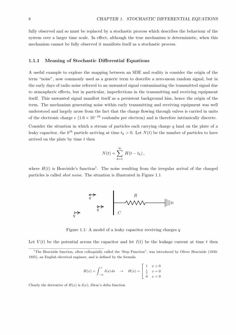
Consider the situation in which a stream of particles each carrying charge q land on the plate of a
leaky capacitor, the kth particle arriving at time tk > 0. Let N(t) be the number of particles to have
arrived on the plate by time t then
N(t) =
∞∑k=1
H(t− tk) ,
where H(t) is Heaviside’s function1. The noise resulting from the irregular arrival of the charged
particles is called shot noise. The situation is illustrated in Figure 1.1
R
C
q
q
q
Figure 1.1: A model of a leaky capacitor receiving charges q
Let V (t) be the potential across the capacitor and let I(t) be the leakage current at time t then
1The Heaviside function, often colloquially called the ‘Step Function”, was introduced by Oliver Heaviside (1850-
1925), an English electrical engineer, and is defined by the formula
H(x) =
∫ x
−∞δ(s) ds → H(x) =
1 x > 012
x = 0
0 x < 0
Clearly the derivative of H(x) is δ(x), Dirac’s delta function
1.1. INTRODUCTION 9
conservation of charge requires that
CV = q N(t)−∫ t
0I(s) ds
where V (t) = RI(t) by Ohms law. Consequently, I(t) satisfies the integral equation
CRI(t) = q N(t)−∫ t
0I(s) ds . (1.1)
We can solve this equation by the method of Laplace transforms, but we avoid this temptation.
Another approach
Consider now the nature of N(t) when the times tk are unknown other than that electrons behave
independently of each other and that the interval between the arrivals of electrons of the plate is
Poisson distributed with parameter λ. With this understanding of the underlying mechanism in
place, N(t) is a Poisson deviate with parameter λt. At time t+∆t equation (1.1) becomes
CRI(t+∆t) = q N(t+∆t)−∫ t+∆t
0I(s) ds .
After subtracting equation (1.1) from the previous equation the result is that
CR [I(t+∆t)− I(t)] = q [N(t+∆t)−N(t)]−∫ t+∆t
tI(s) ds . (1.2)
Now suppose that ∆t is sufficiently small that I(t) does not change its value significantly in the
interval [t, t+∆t] then ∆I = I(t+∆t)− I(t) and∫ t+∆t
tI(s) ds ≈ I(t)∆t .
On the other hand suppose that ∆t is sufficiently large that many electrons arrive on the plate
during the interval (t, t+∆t). So although [N(t+∆t)−N(t)] is actually a Poisson random variable
with parameter λ∆t, the central limit theorem may be invoked and [N(t + ∆t) − N(t)] may be
approximated by a Gaussian deviate with mean value λ∆t and variance λ∆t. Thus
N(t+∆t)−N(t) ≈ λ∆t+ λ∆W , (1.3)
where ∆W is a Gaussian random variable with zero mean value and variance ∆t. The sequence of
values for ∆W as time is traversed in units of ∆t define the independent increments in a Gaussian
processW (t) formed by summing the increments ∆W . ClearlyW (t) has mean value zero and variance
t. The conclusion of this analysis is that
CR∆I = q (λ∆t+√λ∆W )− I(t)∆t (1.4)
with initial condition I(0) = 0. Replacing ∆I, ∆t and ∆W by their respective differential forms
leads to the Stochastic Differential Equation (SDE)
dI =(qλ− I)
CRdt+
q√λ
CRdW . (1.5)
In this representation, dW is the increment of a Wiener process. Both I and W are functions which
are continuous everywhere but differentiable nowhere. Equation (1.5) is an example of an Ornstein-
Uhlenbeck process.
10 CHAPTER 1. STOCHASTIC DIFFERENTIAL EQUATIONS
1.2 Some applications of SDEs
1.2.1 Asset prices
The most relevant application of SDEs for our purposes occurs in the pricing of risky assets and
contracts written on these assets. One such model is Heston’s model of stochastic volatility which
posits that S, the price of a risky asset, evolves according to the equations
dS
S= µdt+
√V (
√1− ρ2 dW1 + ρ dW2)
dV = κ (γ − V ) dt+ σ√V dW2
(1.6)
in which ρ, κ and γ take prescribed values and V (t) is the instantaneous level of volatility of the
stock, and dW1 and dW2 are differentials of uncorrelated Wiener processes. In the course of these
lectures we shall meet other financial models.
1.2.2 Population modelling
Stochastic differential equations are often used in the modelling of population dynamics. For example,
the Malthusian model of population growth (unrestricted resources) is
dN
dt= aN , N(0) = N0 , (1.7)
where a is a constant and N(t) is the size of the population at time t. The effect of changing
environmental conditions is achieved by replacing a dt by a Gaussian random variable with non-zero
mean a dt and variance b2 dt to get the stochastic differential equation
dN = aN dt+ bN dW , N(0) = N0 , (1.8)
in which a and b (conventionally positive) are constants. This is the equation of a Geometric Random
Walk and is identical to the risk-neutral asset model proposed by Black and Scholes for the evolution
of the price of a risky asset. To take account of limited resources the Malthusian model of population
growth is modified by replacing a in equation (1.8) by the term α(M − N) to get the well-known
Verhulst or Logistic equation
dN
dt= αN(M −N) , N(0) = N0 (1.9)
where α and M are constants with M representing the carrying capacity of the environment. The
effect of changing environmental conditions is to make M a stochastic parameter so that the logistic
model becomes
dN = aN(M −N) dt+ bN dW (1.10)
in which a and b ≥ 0 are constants.
1.2. SOME APPLICATIONS OF SDES 11
The Malthusian and Logistic models are special cases of the general stochastic differential equation
dN = f(N) dt+ g(N) dW (1.11)
where f and g are continuously differentiable in [0,∞) with f(0) = g(0) = 0. In this case, N = 0 is a
solution of the SDE. However, the stochastic equation (1.11) is sensible only provided the boundary
at N = ∞ is unattainable (a natural boundary). This condition requires that there exist K > 0 such
that f(N) < 0 for all N > K. For example, K =M in the logistic model.
1.2.3 Multi-species models
The classical multi-species model is the prey-predator model. Let R(t) and F (t) denote respectively
the populations of rabbits and foxes is a given environment, then the Lotka-Volterra two-species
model posits thatdR
dt= R(α− β F )
dF
dt= F (δ R− γ) ,
where α is the net birth rate of rabbits in the absence of foxes, γ is the natural death rate of foxes
and β and δ are parameters of the model controlling the interaction between rabbits and foxes. The
stochastic equations arising from allowing α and γ to become random variables are
dR = R(α− β F ) dt+ σr RdW1 .
dF = F (δ R− γ) dt+ σf F dW2 .
The generic solution to these equations is a cyclical process in which rabbits dominate initially,
thereby increasing the supply of food for foxes causing the fox population to increase and rabbit
population to decline. The increasing shortage of food then causes the fox population to decline and
allows the rabbit population to recover, and so on.
There is a multi-species variant of the two-species classical Lotka-Volterra multi-species model with
differential equationsdxkdt
= (ak + bkjxj)xk , k n.s. , (1.12)
where the choice and algebraic signs of the ak’s and the bjk’s distinguishes prey from predator. The
simplest generalisation of the Lotka-Volterra model to stochastic a environment assumes the original
ak is stochastic to get
dxk = (ak + bkjxj)xk dt+ ck xk dWk , k not summed. (1.13)
The generalised Lokta-Volterra models also have cyclical solutions. Is there an analogy with business
cycles in Economics in which the variables xk now denote measurable economic variables?
12 CHAPTER 1. STOCHASTIC DIFFERENTIAL EQUATIONS
Chapter 2
Continuous Random Variables
2.1 The probability density function
Function f(x) is a probability density function (PDF) with respect to a subset S ⊆ Rn provided
(a) f(x) ≥ 0 ∀ x ∈ S , (ii)
∫Sf(x) dx = 1 . (2.1)
In particular, if E ⊆ S is an event then the probability of E is
p(E) =
∫Ef(x) dx .
2.1.1 Change of independent deviates
Suppose that y = g(x) is an invertible mapping which associates X ∈ SX with Y ∈ SY where SY is
the image of the original sample space SX under the mapping g. The probability density function
fY (y) of Y may be computed from the probability density function fX(x) of X by the rule
fY (y) = fX(x)∣∣∣ ∂(x1, · · · , xn)∂(y1, · · · , yn)
∣∣∣ . (2.2)
2.1.2 Moments of a distribution
Let X be a continuous random variable with sample space S and PDF f(x) then the mean value of
the function g(X) is defined to be
g =
∫Sg(x)f(x) dx .
Important properties of the distribution itself are defined from this definition by assigning various
scalar, vector of tensorial forms to g. The momentMpq···w of the distribution is defined by the formula
Mp q···w = E [XpXq · · ·Xw ] =
∫S(xpxq · · ·xw) f(x) dx . (2.3)
13
14 CHAPTER 2. CONTINUOUS RANDOM VARIABLES
2.2 Ubiquitous probability density functions in continuous finance
Although any function satisfying conditions (2.1) qualifies as a probability density function, there
are several well-known probability density functions that occur frequently in continuous finance and
with which one must be familiar. These are now described briefly.
2.2.1 Normal distribution
A continuous random variable X is Gaussian distributed with mean µ and variance σ2 if X has
probability density function
f(x) =1√2πσ
exp[− (x− µ)2
2σ2
].
Basic properties
• If X ∼ N(µ, σ2) then Y = (X − µ)/σ ∼ N(0, 1) . This result follows immediately by change of
independent variable from X to Y .
• Suppose that Xk ∼ N(µk, σ2k) for k = 1, . . . , n are n independent Gaussian deviates then
mathematical induction may be used to establish the result
X = X1 +X2 + . . .+Xn ∼ N( n∑k=1
µk ,n∑k=1
σ2k
).
2.2.2 Log-normal distribution
The log-normal distribution with parameters µ and σ is defined by the probability density function
f(x ; µ, σ) =1√2π σ
1
xexp
[− (log x− µ)2
2σ2
]x ∈ (0,∞) (2.4)
Basic properties
• If X is log-normally distributed with parameters (µ, σ) then Y = logX ∼ N(µ, σ2). This result
follows immediately by change of independent variable from X to Y .
• If X is log-normally distributed with parameters (µ, σ) independent Gaussian deviates then
E [X] = eµ+σ2/2 and V [X] = e2µ+σ
2(eσ
2 − 1) and the median of X is eµ.
2.2.3 Gamma distribution
The Gamma distribution with shape parameter α and scale parameter λ is defined by the probability
density function
f(x) =1
λΓ(α)
(xλ
)α−1e−x/λ ,
2.3. LIMIT THEOREMS 15
where λ and α are positive parameters.
Basic properties
• If X is Gamma distributed with parameters (α, λ) then E [X] = αλ and V [X] = αλ2.
• Suppose that X1, · · · , Xn are n independent Gamma deviates such that Xk has shape parameter
αk and scale parameter λ, the same for all values of k, then mathematical induction may be
used to establish the result that X = X1 + X2 + . . . + Xn is Gamma distributed with shape
parameter α1 + α2 + · · ·+ αn and scale parameter λ.
2.3 Limit Theorems
“Limit Theorems” are arguably the most important theoretical results in probability. The results
come in two flavours:
(i) Laws of Large Numbers where the aim is to establish convergence results relating sample
and population properties. For example, how many times must one toss a coin to be 99% sure
that the relative frequency of heads is within 5% of the true bias of the coin.
(ii) Central Limit Theorems where the aim is to establish properties of the distribution of the
sample properties.
Subsequent statements will assume that X1, X2, . . . , Xn is a sample of n independent and identically
distributed (i.i.d.) random variables. The sum of the random variables in the sample will be denoted
by Sn = X1 + · · ·+Xn. There are three different ways in which a random sequence Yn can converge
to, say T , as n→ ∞.
Definition
(a) We say that Yn → Y strongly as n→ ∞ if
Prob ( |Yn − Y | → 0 as n→ ∞ ) = 1 .
(b) We say that Yn → Y as n→ ∞ in the mean square sense if
∥Yn − Y ∥ =√
E [ (Yn − Y )2 ] → 0 as n→ ∞ .
(c) We say that Yn → Y weakly as n→ ∞ if given ε > 0,
Prob ( |Yn − Y | ≥ ε ) → 0 as n→ ∞ .
Weak convergence (sometimes called stochastic convergence) is the weakest convergence condi-
tion. Strong convergence and mean square convergence both imply weak convergence.
16 CHAPTER 2. CONTINUOUS RANDOM VARIABLES
Before considering specific limit theorems, we establish Chebyshev’s inequality.
Chebyshev’s inequality
Let g(x) be a non-negative function of a continuous random variable X then
Prob ( g(X) > K ) <E [ g(X) ]
K.
Justification Let X have pdf f(x) then
E [ g(X) ] =
∫g(x) f(x) dx ≥ K
∫g(x)≥K
f(x) dx = K Prob ( g(X) > K ) .
Chebyshev’s inequality follows immediately from this result.
Corollary
Let X be a random variable drawn from a distribution with finite mean µ and finite variance σ2 then
it follows directly from Chebyshev’s inequality that
Prob ( |X − µ | > ϵ) ≤ σ2
ϵ2.
Justification Take g(x) = (X − µ)2/σ2 and K = ε2/σ2. Clearly E [ g(X) ] = 1 and Chebyshev’s
inequality now gives
Prob ( (X − µ)2/σ2 > ε2/σ2 ) <σ2
ε2→ Prob ( |X − µ | > ε ) <
σ2
ε2.
The weak law of large numbers
Let X1, X2, . . . , Xn be a sample of n i.i.d random variables drawn from a distribution with finite
mean µ and finite variance σ2, then for any positive ϵ
Prob
( ∣∣∣∣Snn − µ
∣∣∣∣ > ϵ
)→ 0 as n→ ∞ .
Justification To establish this result, apply Chebyshev’s inequality with X = Sn/n. In this case
E(X) = µ and σ2X = σ2/n. It follows directly from Chebyshev’s inequality that
p(|X − µ| > ϵ) ≤ σ2
nϵ2→ 0 as n→ ∞ .
The strong law of large numbers
Let X1, X2, . . . , Xn be a sample of n i.i.d random variables drawn from a distribution with finite
mean µ and finite variance σ2, then
Snn
→ µ as n→ ∞ w.p. 1 .
[In fact, the finite variance condition is not necessary for the strong law of large numbers to be true.]
2.4. THE WIENER PROCESS 17
2.3.1 The central limit results
Let X1, X2, . . . Xn be a sample of n i.i.d. random variables from a distribution with finite mean µ
and finite variance σ2, then the random variable
Yn =Sn − nµ
σ√n
has mean value zero and unit variance. In particular, the unit variance property means that Yn does
not degenerate as n → ∞ by contrast with Sn/n. The law of the iterated logarithm controls the
growth of Yn as n→ ∞.
Central limit theorem
Under the conditions on X stated previously, the derived deviate Yn satisfies
limn→∞
Prob (Yn ≤ y ) =1√2π
∫ y
−∞e−t
2/2 dt .
The crucial point to note here is that the result is independent of distribution provided each deviate
Xk is i.i.d. with finite mean and variance. For example, The strong law of large numbers would
apply to samples drawn from the distribution with density f(x) = 2(1+x)−3 with x ∈ R but not the
central limit theorem.
2.4 The Wiener process
In 1827 the Scottish botanist Robert Brown (1773-1858) first described the erratic behaviour of
particles suspended in fluid, an effect which subsequently came to be called “Brownian Motion”. In
1905 Einstein explained Brownian motion mathematically1 and this led to attempts by Langevin and
others to formulate the dynamics of this motion in terms of stochastic differential equations. Norbert
Wiener (1894-1964) introduced a mathematical model of Brownian motion based on a canonical
process which is now called the Wiener process.
The Wiener process, denoted W (t) t ≥ 0, is a continuous stochastic process which takes the initial
value W (0) = 0 with probability one and is such that the increment [W (t) −W (s)] from W (s) to
W (t) (t > s) is an independent Gaussian process with mean value zero and variance (t− s). If Wt is
a Wiener process, then
∆Wt =Wt+∆t −Wt
is a Gaussian process satisfying
E [∆Wt ] = 0 , V [∆Wt ] = ∆t . (2.5)
1The canonical equation is called the diffusion equation, written
∂θ
∂t=
∂2θ
∂x2
in one dimension. It is classified as a parabolic partial differential equation and typically describes the evolution of
temperature in heated material.
18 CHAPTER 2. CONTINUOUS RANDOM VARIABLES
It is often convenient to write ∆Wt =√∆t ϵt for the increment experienced by the Wiener process
W (t) in traversing the interval [t, t+∆t] where ϵt ∼ N(0, 1). Similarly, the infinitesimal increment dW
inW (t) during the increment dt is often written dW =√dt ϵt. Suppose that t = t0 < · · · < tn = t+T
is a dissection of [t, t+ T ] then
W (t+ T )−W (t) =
n∑k=1
[W (tk)−W (tk−1) ] =
n∑k=1
√(tk − tk−1) ϵk , ϵk ∼ N(0, 1) . (2.6)
Note that this incremental form allows the mean and variance properties of the Wiener process to
be established directly from the properties of the Gaussian distribution.
2.4.1 Covariance
Let t and s be times with t > s then
E [W (t)W (s) ] = E [W (s)(W (t)−W (s)) +W 2(s) ] = E [W 2(s) ] = s . (2.7)
In the derivation of result (2.7) it has been recognised that W (s) and the Wiener increment W (t)−W (s) are independent Gaussian deviates. In general, E [W (t)W (s) ] = min(t, s).
2.4.2 Derivative of a Wiener process
The formal derivative of the Wiener process W (t) is the limiting value of the ratio
lim∆t→0
W (t+∆t)−W (t)
∆t. (2.8)
However W (t+∆t)−W (t) =√∆t ϵt and so
W (t+∆t)−W (t)
∆t=
ϵt√∆t
.
Thus the limit (2.8) does not exist as ∆t→ 0+ and so W (t) has no derivative in the classical sense.
Intuitively this means that a particle with position x(t) =W (t) has no well defined velocity although
its position is a continuous function of time.
2.4.3 Definitions
1. A martingale is a gambling term for a fair2 game in which the current information set It pro-
vides no advantage in predicting future winnings. A random variable Xt with finite expectation
is a martingale with respect to the probability measure P if
E P [Xt+s | It ] = Xt , s > 0 . (2.9)
2Of course, martingale gambling strategies are an anathema to casinos; this is the primary reason for a house limit
which, of course, precludes martingale strategies.
2.4. THE WIENER PROCESS 19
Thus the future expectation of X is its current value, or put another way, the future offers no
opportunity for arbitrage.
2. A random variable Xt with finite expectation is said to be a sub-martingale with respect to
the probability Q if
EQ [Xt+s | It ] ≥ Xt , s > 0 . (2.10)
3. Let t0 < t1 · · · < t · · · be an increasing sequence of times with corresponding information sets
I0, I1, · · · , It, · · ·. These information sets are said to form a filtration if
I0 ⊆ I1 ⊆ · · · ⊆ It ⊆ · · · (2.11)
For example, Wt =W (t) is a martingale with respect to the information set I0. Why? Because
E [Wt | I0 ] = 0 =W (0) ,
but W 2t is a sub-martingale since E [W 2
t | I0 ] = t > 0.

20 CHAPTER 2. CONTINUOUS RANDOM VARIABLES
Chapter 3
Review of Integration
Before advancing to the discussion of stochastic differential equations, we need to review what is
meant by integration. Consider briefly the one-dimensional SDE
dxt = a(t, xt) dt+ b(t, xt) dWt , x(t0) = x0 , (3.1)
where dWt is the differential of the Wiener process W (t), and a(t, x) and b(t, x) are deterministic
functions of x and t. The motivation behind this choice of direction lies in the observation that the
formal solution to equation (3.1) may be written
xt = x0 +
∫ t
t0
a(s, xs) ds+
∫ t
t0
b(s, xs) dWs . (3.2)
Although this solution contains two integrals, to have any worth we need to know exactly what is
meant by each integral appearing in this solution.
At a casual glance, the first integral on the right hand side of solution (3.2) appears to be a Riemann
integral while the second integral appears to be a Riemann-Stieltjes integral. However, a complication
arises from the fact that xs is a stochastic process and so a(s, xs) and b(s, xs) behave stochastically
in the integrals although a and b are themselves deterministic functions of t and x.
In fact, the first integral on the right hand side of equation (3.2) can always be interpreted as a
Riemann integral. However, the interpretation of the second integral is problematic. Often it is an
Ito integral, but may be interpreted as a Riemann-Stieltjes integral under some circumstances.
3.1 Bounded Variation
Let Dn denote the dissection a = x0 < x1 < · · · < xn = b of the finite interval [a, b]. The p-variation
of a function f over the domain [a, b] is defined to be
Vp(f) = limn→∞
n∑k=1
| f(xk)− f(xk−1) |p , p > 0 , (3.3)
21
22 CHAPTER 3. REVIEW OF INTEGRATION
where the limit is taken over all possible dissections of [a, b]. The function f is said to be of bounded
p-variation if Vp(f) < M < ∞. In particular, if p = 1, then f is said to be a function of bounded
variation over [a, b]. Clearly if f is of bounded variation over [a, b] then f is necessarily bounded in
[a, b]. However the converse is not true; not all functions which are bounded in [a, b] have bounded
variation.
Suppose that f has a finite number of maxima and minima within [a, b], say a < ξ1 < · · · < ξm < b.
Consider the dissection formed from the endpoints of the interval and the m ordered maxima and
minima of f . In the interval [ξk−1, ξk], the function f either increases or decreases. In either event,
the variation of f over [ξk−1, ξk] is | f(ξk)− f(ξk−1) | and so the variation of f over [a, b] is
m∑k=0
| f(ξk+1)− f(ξk) | <∞ .
Let Dn be any dissection of [a, b] and suppose that xk−1 ≤ ξj ≤ xk, then the triangle inequality
| f(xk)− f(xk−1) | = | [ f(xk)− f(ξj) ] + [ f(ξj)− f(xk−1) ] |
≤ | f(xk)− f(ξj) |+ | f(ξj)− f(xk−1) |
ensures that
V (f) = limn→∞
n∑k=1
| f(xk)− f(xk−1) | ≤m∑k=0
| f(ξk+1)− f(ξk) | <∞ . (3.4)
Thus f is a function of bounded variation. Therefore to find functions which are bounded but are
not of bounded variation, it is necessary to consider functions which have at least a countable family
of maxima and minima. Consider, for example,
f(x) =
sin(π/x) x > 0
0 x = 0
and let Dn be the dissection with nodes x0 = 0, xk = 2/(2n− 2k + 1) when 1 ≤ k ≤ n− 1 and with
xn = 1. Clearly f(x0) = f(xn) = 0 while f(xk) = sin((n − k)π + π/2) = (−1)n−k. The variation of
f over Dn is therefore
Vn(f) =
n∑k=1
| f(xk)− f(xk−1) |
= | f(x0)− f(x1) |+ · · · | f(xk)− f(xk−1) |+ · · · | f(xn)− f(xn−1) |
= 1 + 2 · · · (n− 2) times · · ·+ 2 + 1
= 2(n− 1)
Thus f bounded in [0, 1] but is not a function of bounded variation in [0, 1].
3.2. RIEMANN INTEGRATION 23
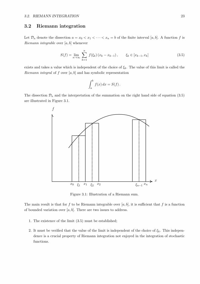
3.2 Riemann integration
Let Dn denote the dissection a = x0 < x1 < · · · < xn = b of the finite interval [a, b]. A function f is
Riemann integrable over [a, b] whenever
S(f) = limn→∞
n∑k=1
f(ξk) (xk − xk−1) , ξk ∈ [xk−1, xk] (3.5)
exists and takes a value which is independent of the choice of ξk. The value of this limit is called the
Riemann integral of f over [a, b] and has symbolic representation∫ b
af(x) dx = S(f) .
The dissection Dn and the interpretation of the summation on the right hand side of equation (3.5)
are illustrated in Figure 3.1.
x0 x1 x2 xnξ1 ξ2 ξn−1
x
f
Figure 3.1: Illustration of a Riemann sum.
The main result is that for f to be Riemann integrable over [a, b], it is sufficient that f is a function
of bounded variation over [a, b]. There are two issues to address.
1. The existence of the limit (3.5) must be established;
2. It must be verified that the value of the limit is independent of the choice of ξk. This indepen-
dence is a crucial property of Riemann integration not enjoyed in the integration of stochastic
functions.
24 CHAPTER 3. REVIEW OF INTEGRATION
Independence of limit
Let η(L)k and η
(U)k be respectively the values of x ∈ [xk−1, xk] at which f attains its minimum and
maximum values. Thus f(η(L)k ) ≤ f(ξk) ≤ f(η
(U)k ). Let S(L)(f) and S(U)(f) be the values of the limit
(3.5) in which ξk takes the respective values η(L)k and η
(U)k then
S(L)n (f) =
n∑k=1
f(η(L)k )(xk − xk−1) ≤
n∑k=1
f(ξk)(xk − xk−1) ≤n∑k=1
f(η(U)k )(xk − xk−1) = S(U)
n (f) .
Assuming the existence of limit (3.5) for all choices of ξ, it therefore follow that
S(L)(f) ≤ S(f) ≤ S(U)(f) (3.6)
where S(f) is the value of the limit (3.5) in which the sequence of ξ values are arbitrary. In particular,
|S(U)n (f)− S(L)
n (f) | =∣∣∣ n∑k=1
f(η(U)k )(xk − xk−1)−
n∑k=1
f(η(L)k )(xk − xk−1)
∣∣∣=
∣∣∣ n∑k=1
(f(η
(U)k )− f(η
(L)k )
)(xk − xk−1)
∣∣∣≤
n∑k=1
| f(η(U)k )− f(η
(L)k )| (xk − xk−1)
Suppose now that ∆n is the length of the largest sub-interval of Dn then it follows that
|S(U)n (f)− S(L)
n (f) | ≤ ∆n
n∑k=1
| f(η(U)k )− f(η
(L)k )| ≤ ∆n V (f) . (3.7)
Since f is a function of bounded variation over [a, b] then V (f) < M < ∞. On taking the limit of
equation (3.7) as n→ ∞ and using the fact that ∆n → 0, it is seen that S(U)(f) = S(L)(f).
3.3 Riemann-Stieltjes integration
Riemann-Stieltjes integration is similar to Riemann integration except that summation is now per-
formed with respect to g, a function of x, rather than x itself. For example, if F is the cumulative
distribution function of the random variable X, then one definition for the expected value of X is
the Riemann-Stieltjes integral
E [X ] =
∫ b
ax dF (3.8)
in which x is integrated with respect to F .
Let Dn denote the dissection a = x0 < x1 < · · · < xn = b of the finite interval [a, b]. The Riemann-
Stieltjes integral of f with respect to g over [a, b] is defined to be the value of the limit
limn→∞
n∑k=1
f(ξk) [ g(xk)− g(xk−1) ] , ξk ∈ [xk−1, xk] (3.9)
3.4. STOCHASTIC INTEGRATION OF DETERMINISTIC FUNCTIONS 25
when this limit exists and takes a value which is independent of the choice of ξk and the limiting
properties of the dissectionDn. Young has shown that the conditions for the existence of the Riemann-
Stieltjes integral are met provided the points of discontinuity of f and g in [a, b] are disjoint, and
that f is of p-variation and g is of q variation where p > 0, q > 0 and p−1 + q−1 > 1.
Note that neither f nor g need be continuous functions, and of course, when g is a differentiable
function of x then the Riemann-Stieltjes of f with respect to g may be replaced by the Riemann
integral of fg′ provided fg′ is a function of bounded variation on [a, b]. So in writing down the
prototypical Riemann-Stieltjes integral ∫f dg
it is usually assumed that g is not a differentiable function of x.
3.4 Stochastic integration of deterministic functions
The discussion of stochastic differential equations will involve the treatment of integrals of type∫ b
af(t) dWt (3.10)
in which f is a deterministic function of t. To determine what conditions must be imposed on f
to guarantee the existence of this Riemann-Stieltjes integral, it is necessary to determine the value
of p for which Wt is of bounded p-variation. Consider the interval [t, t + h] and the properties of
|W (t+ h)−W (t)|p.
Let X = Wt+h −Wt ∼ N(0, h) and let Y = |Wt+h −Wt|p = |X|p. The sample space of Y is [0,∞)
and fY (y), the probability density function of Y , satisfies
fY (y) = 2 fXdx
dy=
2y1/p−1
p√2π h
e−x2/2h =
√2
π h
y1/p−1
pe−y
2/p/2h ,
where x = y1/p. If p = 2, then
fY (y) =
√1
2π hy−1/2 e−y/2h
making Y a gamma deviate with scale parameter λ = 2h and shape parameter α = 1. Otherwise,
E [Y ] = µ =
∫ ∞
0
√2
π h
y1/p
pe−y
2/p/2h =1
p
√2
π h
∫ ∞
0y1/p e−y
2/p/2h =(2h)p/2√
πΓ( p+ 1
2
),
and the variance of Y is
V [Y ] =
∫ ∞
0
√2
π h
y1/p+1
pe−y
2/p/2h − µ2
=1
p
√2
π h
∫ ∞
0y1/p+1 e−y
2/p/2h − µ2
=(2h)p√π
Γ(p+
1
2
)− µ2 =
(2h)p√π
[Γ(p+
1
2
)− 1√
πΓ2
( p+ 1
2
) ].
26 CHAPTER 3. REVIEW OF INTEGRATION
The process of forming the p-variation of the Wiener process Wt requires the summation of objects
such as |Wt+h−Wt|p in which the values of h are simply the lengths of the intervals of the dissection,
i.e. over the interval [0, T ] the p-variation of Wt requires the investigation of the properties of
V (p)n (W ) =
n∑k=1
|W (tk+1)−W (tk)|p , tk+1 − tk = hk h1 + h2 + · · ·+ hn = T
and for Wt to be of p-variation on [0, T ], the limit of V(p)n (W ) must be finite for all dissections as
n→ ∞. Consider however the uniform dissection in which h1 = · · · = hn = T/n. In this case
E[V (p)n (W )] =
n∑k=1
E[|W (tk+1)−W (tk)|p] =(2T )p/2√
πΓ( p+ 1
2
)n1−p/2 ,
If p < 2, the expected value E[V (p)n (W )] is unbounded and so Wt cannot be of p-variation when
p < 2. When p = 2 it is clear that E[V (p)n (W )] = T . For general dissection Dn the distribution of
V(2)n (W ) is unclear but when h1 = · · · = hn = T/n the function V
(2)n (W ) is chi-squared distributed
being the sum of the squares of n independent and identically distributed Gaussian random deviates.
The expected value of each term in the sum required to form the p-variation of Wt always exceeds
a constant multiple of 1/np/2 and therefore the sum of these expected values diverges for all p ≤ 2
and converges for p > 2. The variance of the p-variation behaves like a sum of terms with behaviour
1/np, and always converges. Thus the Wiener process is of bounded p-variation for p > 2.
Consequently, the properties of the Riemann-Stieltjes integral (3.8) guarantee that the stochastic
integral (3.10) is defined as a Riemann-Stieltjes integral for all functions f with bounded q-variation
where q < 2. Clearly functions of bounded variation (q = 1) satisfy this condition, and therefore if f
is Riemann integrable over [a, b], then the the stochastic integral (3.10) exists and can be treated as
a Riemann-Stieltjes integral.
Chapter 4
The Ito and Stratonovich Integrals
4.1 A simple stochastic differential equation
To motivate the Ito and Stratonovich integrals, consider the generic one dimensional SDE
dxt = a(t, xt) dt+ b(t, xt) dWt (4.1)
where dWt is the increment of the Wiener process, and a(t, x) and b(t, x) are deterministic functions of
x and t. Of course, a and b behave randomly in the solution of the SDE by virtue of their dependence
on x. The meanings of a(t, x) and b(t, x) become clear from the following argument.
Since E [ dWt ] = 0, it follows directly from equation (4.1) that E [ dx ] = a(t, x) dt. For this reason,
a(t, x) is often called the drift component of the stochastic differential equation. One usually regards
the equation dx/dt = a(t, x) as the genitor differential equation from which the SDE (4.1) is born.
This was precisely the procedure used to obtain SDEs from ODEs in the introductory chapter.
Furthermore,
V (dx) = E [ (dx− a(t, x) dt)2 ] = E [ b(t, x) dW 2t ] = b(t, x) E [ dW 2
t ] = b2(t, x) dt . (4.2)
Thus b2(t, x) dt is the variance of the stochastic process dx and therefore b2(t, x) is the rate at which
the variance of the stochastic process grows in time. The function b2(t, x) is often called the diffusion
of the SDE and b(t, x), being dimensionally a standard deviation, is usually called the volatility of
the SDE. In effect, an ODE is an SDE with no volatility.
Note, however, that the definition of the terms a(t, x) and b(t, x) should not be confused with the
idea that the solution to an SDE simply behaves like the underlying ODE dx/dt = a(t, x) with
superimposed noise of volatility b(x, t) per unit time. In fact, b(x, t) contributes to both drift and
variance. Therefore, one cannot estimate the parameters of an SDE by treating the drift (determin-
istic behaviour of the solution) and volatility (local variation of solution) as separate processes.
27
28 CHAPTER 4. THE ITO AND STRATONOVICH INTEGRALS
4.1.1 Motivation for Ito integral
It has been noted previously that the solution to equation (4.1) has formal expression
x(t) = x(s) +
∫ t
sa(r, xr) dr +
∫ t
sb(r, xr) dWr , t ≥ s , (4.3)
where the task is now to state how each integral on the right hand side of equation (4.3) is to be
computed. Consider the computation of the integrals in (4.3) over the interval [t, t + h] where h
is small. Assuming that xt is a continuous random function of t and that a(t, x) and b(t, x) are
continuous functions of (t, x), then a(r, xr) and b(r, xr) in (4.3) may be approximated by a(t, xt) and
b(t, xt) respectively to give
x(t+ h) ≈ x(t) + a(t, xt)
∫ t+h
tdr + b(t, xt)
∫ t+h
tdWr ,
= x(t) + a(t, xt)h+ b(t, xt) [W (t+ h)−W (t) ] .
(4.4)
Note, in particular, that E [ b(t, xt) (W (t+ h)−W (t) ] = 0 and therefore the stochastic contribution
to the solution (4.4) is a martingale1, that is, it is non-anticipative. This solution intuitively agrees
with ones conceptual picture of the future, namely that ones best estimate of the future is the current
state plus a drift which, of course, is deterministic.
This simple approximation procedure (which will subsequently be identified as the Euler-Maruyama
approximation) is consistent with the view that the first integral on the right hand side of (4.3) is a
standard Riemann integral. On the other hand, the second integral on the right hand side of (4.3)
is a stochastic integral with the martingale property, that is, it is a non-anticipative random variable
with expected value zero - the value when h = 0. Let s = t0 < t1 < · · · < tn = t be a dissection of
[s, t]. The extension of the approximation procedure used in the derivation of (4.4) to the interval
[s, t] suggests the definition
∫ t
sb(r, xr) dWr = lim
n→∞
n−1∑k=0
b(tk, x(tk)) [W (tk+1)−W (tk) ] . (4.5)
This definition automatically endows the stochastic integral with the martingale property - the reason
is that b(tk, xk) depends on the behaviour of the Wiener process in (s, tk) alone and so the value of
b(tk, xk) is independent of W (tk+1)−W (tk).
In fact, the computation of the stochastic integral in equation (4.5) is based on the mean square
1A martingale refers originally to a betting strategy popular in 18th century France in which the expected winnings
of the strategy is the original stake. The simplest example of a martingale is the double or quit strategy in which a
bet is doubled until a win is achieved. In this strategy the total loss after n unsuccessful bets is (2n − 1)S where S is
the original stake. The bet at the (n + 1)-th play is 2n S so that the first win necessarily recovers all previous losses
leaving a profit of S. Since a gambler with unlimited wealth eventually wins, devotees of the martingale betting strategy
regarded it as a sure-fire winner. In reality, however, the exponential growth in the size of bets means that gamblers
rapidly become bankrupt or are prevented from executing the strategy by the imposition of a maximum bet.
4.2. STOCHASTIC INTEGRALS 29
limiting process. More precisely, the Ito Integral of b(t, xt) over [a, b] is defined by
limn→∞
E[ n∑k=1
b(tk−1 , xk−1) (Wk −Wk−1 )−∫ b
ab(t, xt) dWt
]2= 0 , (4.6)
where xk = x(tk) and Wk = W (tk). The limiting process in (4.6) defines the Ito integral of b(t, xt)
(assuming that xt is known), and the computation of integrals defined in this way is called Ito
Integration. Most importantly, the Ito integral is a martingale, and stochastic differential equations
of the type (4.1) are more correctly called Ito stochastic differential equations.
In particular, the rules for Ito integration can be different from the rules for Riemann/Riemann-
Stieltjes integration. For example,∫ t
sdWr =W (t)−W (s) , but
∫ t
sWr dWr =
W 2(t)−W 2(s)
2.
To appreciate why the latter result is false, simply note that
E[ ∫ t
sWr dWr
]= 0 = E
[W 2(t)−W 2(s)
2
]=t− s
2> 0 .
Clearly the Riemann-Stieltjes integral is a sub-martingale, but what has gone wrong with the
Riemann-Stieltjes integral in the previous illustration is the crucial question. Suppose one considers∫ t
sWr dWr
within the framework of Riemann-Stieltjes integration with f(t) = W (t) and g(t) = W (t). The
key observation is that W (t) is of p-variation with p > 2 and therefore p−1 + q−1 < 1 in this
case. Although this observation is not helpful in evaluating this integral (if indeed it has a value),
the fact that inequality p−1 + q−1 > 1 fails indicates that the integral cannot be interpreted as a
Riemann-Stieltjes integral. Clearly the rules of Ito-Calculus are quite different from those of Liebnitz’s
Calculus.
4.2 Stochastic integrals
The findings of the previous section suggest that special consideration must be given to the compu-
tation of the generic integral ∫ b
af(t,Wt) dWt . (4.7)
While superficially taking the form of a Riemann-Stieltjes, both components of the integrand have
p-variation and q-variation such that p > 2 and q > 2 and therefore p−1 + q−1 < 1. Nevertheless,
expression (4.7) may be assigned a meaning in the usual way. Let Dn denote the dissection a = t0 <
t1 < · · · < tn = b of the finite interval [a, b]. Formally,∫ b
af(t,Wt) dWt = lim
n→∞
n∑k=1
f(ξk,W (ξk))(W (tk)−W (tk−1)
), ξk ∈ [tk−1, tk] (4.8)
30 CHAPTER 4. THE ITO AND STRATONOVICH INTEGRALS
whenever this limit exist. Of course, if ξk ∈ (tk−1, tk) there in general the integral cannot be a
martingale because f(ξk,W (ξk)) encapsulates the behaviour of Wt in the interval [tk−1, ξk], and
therefore the random variable f(ξk,W (ξk)) is not in general independent of W (tk)−W (tk−1). Thus
E [ f(ξk,W (ξk)) (W (tk)−W (tk−1) ) ] = 0 . tk−1 < ξk <= tk .
Pursuing this idea to its ultimate conclusion indicates that the previous integral is a martingale if and
only if ξk = tk−1, because in this case f(ξk,W (ξk)) and W (tk) −W (tk−1) are independent random
variables thereby making the expectation of the integral zero.
To provide an explicit example of this idea, consider the case f(t,Wt) = Wt, that is, compute the
stochastic integral
I =
∫ b
aWt dWt . (4.9)
Let Wk =W (tk), let ξk = tk−1 + λ (tk − tk−1) where λ ∈ [0, 1] then W (ξk) =Wk−1+λ and∫ b
aWt dWt = lim
n→∞
n∑k=1
W (ξk)(W (tk)−W (tk−1)
)= lim
n→∞
n∑k=1
Wk−1+λ(Wk −Wk−1) , (4.10)
It is straightforward algebra to show that
n∑k=1
Wk−1+λ(Wk −Wk−1) =
n∑k=1
1
2
[W 2k −W 2
k−1 − (Wk −Wk−1+λ)2 + (Wk−1+λ −Wk−1)
2]
from which it follows that
n∑k=1
Wk+λ(Wk −Wk−1) =1
2
[W 2k −W 2
k−1 − (Wk −Wk−1+λ)2 + (Wk−1+λ −Wk−1)
2]
=1
2
[W 2n −W 2
0
]+
1
2
n∑k=1
[(Wk−1+λ −Wk−1)
2 − (Wk −Wk−1+λ)2].
Now observe that
E [ (Wk −Wk−1+λ)2] = (1− λ)(tk − tk−1) , E [ (Wk−1+λ −Wk−1)
2] = λ(tk − tk−1)
and also that E[ (Wk −Wk−1+λ)(Wk−1+λ −Wk−1) ] although property will not be needed in what
follows. Evidently
E[ n∑k=1
Wk+λ(Wk −Wk−1)]=b− a
2+
1
2
n∑k=1
(2λ− 1)(tk − tk−1) = λ(b− a) , (4.11)
from which it follows immediately that the integral is a martingale provided λ = 0. The choice λ = 0
(left hand endpoint of dissection intervals) defines the Ito integral. In particular, the value of the
limit defining the integral would appear to depend of the choice of ξk within the dissection Dn.
The choice λ = 1/2 (midpoint of dissection intervals) is called the Stratonovich integral and leads to
a sub-martingale interpretation of the limit (4.8).
4.3. THE ITO INTEGRAL 31
4.3 The Ito integral
The Ito Integral of f(t,Wt) over [a, b] is defined by∫ b
af(t,Wt) dWt = lim
n→∞
n∑k=1
f(tk−1 ,Wk−1) (Wk −Wk−1 ) , (4.12)
where Wk = W (tk) and convergence of the limiting process is measured in the mean square sense,
i.e. in the sense that
limn→∞
E[ n∑k=1
f(tk−1 ,Wk−1) (Wk −Wk−1 )−∫ b
af(t,Wt) dWt
]2= 0 . (4.13)
The direct computation of Ito integrals from the definition (4.13) is now illustrated with reference to
the Ito integral (4.9). Recall that
Sn =
n∑k=1
Wk−1 (Wk −Wk−1 ) =1
2(W 2(b)−W 2(a))− 1
2
n∑k=1
(Wk −Wk−1)2 . (4.14)
It is convenient to note thatWk−Wk−1 =√tk − tk−1 εk where ε1, · · · , εn are n uncorrelated standard
normal deviates. When expressed in this format
Sn =
n∑k=1
Wk−1 (Wk −Wk−1 ) =1
2(W 2(b)−W 2(a))− 1
2
n∑k=1
(tk − tk−1) ε2k ,
which may in turn be rearranged to give
Sn −1
2[W 2(b)−W 2(a)− (b− a)] =
1
2
n∑k=1
(tk − tk−1) (ε2k − 1) . (4.15)
To finalise the calculation of the Ito Integral and establish the mean square convergence of the right
hand side of (4.15) we note that
limn→∞
E[Sn −
1
2[W 2(b)−W 2(a)− (b− a)]
]2=
1
4limn→∞
E[ ( n∑
k=1
(tk − tk−1) (ε2k − 1)
)2 ]=
1
4limn→∞
E[ n∑j,k=1
(tj − tj−1)(tk − tk−1) (ε2k − 1)(ε2j − 1)
]=
1
4limn→∞
n∑k=1
(tk − tk−1)2 E [ (ε2k − 1)2 ]
(4.16)
where the last line reflects the fact that , (ε2k − 1) and (ε2j − 1) are independent zero-mean random
deviates for j = k. Clearly
E [ (ε2k − 1)2 ] = E [ ε4k ]− 2E [ ε2k ] + 1 = 3− 2 + 1 = 2 .
32 CHAPTER 4. THE ITO AND STRATONOVICH INTEGRALS
In conclusion,
limn→∞
E[Sn −
1
2[W 2(b)−W 2(a)− (b− a)]
]2=
1
2limn→∞
n∑k=1
(tk − tk−1)2 = 0 . (4.17)
The mean square convergence of the Ito integral is now established and so∫ b
aWs dWs =
1
2
[W 2(b)−W 2(a)− (b− a)
]. (4.18)
As has already been indicated, the Ito’s definition of a stochastic integral does not obey the rules of
classical Calculus - the term (b−a)/2 would be absent in classical Calculus. The important advantage
enjoyed by the Ito stochastic integral is that it is a martingale.
The correlation formula for Ito integration
Another useful property of Ito integration is the correlation formula which states that if f(t,Wt)
and g(t,Wt) are two stochastic functions then
E[ ∫ b
af(t,Wt) dWt
∫ b
ag(s,Ws) dWs
]=
∫ b
aE [ f(t,Wt) g(t,Wt) ] dt ,
and in the special case f = g, this result reduces to
E[ ∫ b
af(t,Wt) dWt
∫ b
af(s,Ws) dWs
]=
∫ b
aE [ f2(t,Wt) ] dt .
This is a useful result in practice as we shall see later.
Proof The justification of the correlation formula begins by considering the partial sums
S(f)n =
n∑k=1
f(tk−1 ,Wk−1) (Wk −Wk−1 ) , S(g)n =
n∑k=1
g(tk−1 ,Wk−1) (Wk −Wk−1 ) , (4.19)
from which the Ito integral is defined. It follows that
E[ ∫ b
af(t,Wt) dW
∫ b
ag(s,Ws) dWs
]= lim
n→∞
n∑j,k=1
E [ f(tk−1 ,Wk−1) g(tj−1 ,Wj−1)(Wk −Wk−1 ) (Wj −Wj−1 ) ]
(4.20)
The products f(tk−1 ,Wk−1)g(tj−1 ,Wj−1) and (Wk−Wk−1)(Wj−Wj−1) are uncorrelated when j = k,
and so the contributions to the double sum in equation (4.20) arise solely from the case k = j to get
E[ ∫ b
af(t,Wt) dWt
∫ b
ag(t,Wt) dWt
]= lim
n→∞
n∑k=1
E[f(tk−1 ,Wk−1) g(tk−1 ,Wk−1)(Wk−Wk−1 )
2].
4.4. THE STRATONOVICH INTEGRAL 33
From the fact that f(tk−1 ,Wk−1)g(tj−1 ,Wk−1) is uncorrelated with (Wk −Wk−1)2, it follows that
E[f(tk−1 ,Wk−1) g(tk−1 ,Wk−1)(Wk −Wk−1 )
2]= E [ f(tk−1 g(tk−1 ,Wk−1) ] E [ (Wk −Wk−1 )
2 ]
After replacing E [ (Wk −Wk−1 )2 ] by (tk − tk−1), it is clear that
E[ ∫ b
af(t,Wt) dWt
∫ b
ag(t,Wt) dWt
]= lim
n→∞
n∑k=1
E [ f(tk−1 ,Wk−1) g(tk−1 ,Wk−1) ](tk − tk−1) .
The right hand side of the previous equation is by definition the limiting process corresponding to
the Riemann integral of E [ f(tk−1 ,Wk−1) g(tk−1 ,Wk−1)(tk − tk−1) ] over the interval [a, b], which in
turn establishes the stated result that
E[ ∫ b
af(t,Wt) dWt
∫ b
ag(t,Wt) dWt
]=
∫ b
aE [ f(t ,Wt) g(t ,Wt) ] dt . (4.21)
4.3.1 Application
A frequently occurring application of the correlation formula arises when the Wiener process W (t)
is absent from f , i.e. the task is to assign meaning to the integral
ξ =
∫ b
af(t) dWt . (4.22)
in which f(t) is a function of bounded variation. The integral, although clearly interpretable as
an integral of Riemann-Stieltjes type, is nevertheless a random variable with E[ ξ ] = 0 because
E[ dWt ] = 0. Furthermore, by recognising that the value of the integral is the limit of a weighted
sum of independent Gaussian random variables, it is clear that ξ is simply a Gaussian deviate with
zero mean value. To complete the specification of ξ it therefore remains to compute the variance
of the integral in equation (4.22). The correlation formula is useful in this respect and indicates
immediately that
V[ ξ ] =∫ b
af2(t) dt (4.23)
thereby completing the specification of ξ.
4.4 The Stratonovich integral
The fact that Ito integration does not conform to the traditional rules of Riemann and Riemann-
Stieltjes integration makes Ito integration an awkward procedure. One way to circumvent this awk-
wardness is to introduce the Stratonovich integral which can be demonstrated to obey the traditional
rules of integration under quite relaxed condition but, of course, the martingale property of the Ito
integral must be sacrificed in the process. The Stratonovich integral is a sub-martingale. The overall
strategy is that Ito integrals and Stratonovich integrals are related, but that the latter frequently
conforms to the rules of traditional integration in a way to be made precise at a later time.
34 CHAPTER 4. THE ITO AND STRATONOVICH INTEGRALS
Given a suitably differentiable function f(t,Wt), the Stratonovich integral of f with respect to the
Wiener process W (t) (denoted by “”) is defined by∫ b
af(t,Wt) dWt = lim
n→∞
n∑k=1
f(ξk,W (ξk)) (Wk −Wk−1 ) , ξk =tk−1 + tk
2, (4.24)
in which the function f is sampled at the midpoints of the intervals of a dissection, and where the
limiting procedure (as with the Ito integral) is to be interpreted in the mean square sense, i.e. the
value of the integral requires that
limn→∞
E[ n∑k=1
f(ξk ,W (ξk) ) (Wk −Wk−1 )−∫ b
af(t,Wt) dWt
]2= 0 . (4.25)
To appreciate how Stratonovich integration might differ from Ito integration, it is useful to compute∫ b
aWt dWt .
The calculation mimics the procedure used for the Ito integral and begins with the Riemann-Stieltjes
partial sum
Sn =
n∑k=1
Wk−1/2 (Wk −Wk−1 ) (4.26)
where the notation Wk−1+λ = W (tk−1 + λ(tk − tk−1) ) has been used for convenience. This sum in
now manipulated into the equivalent algebraic form
1
2
[ n∑k=1
(W 2k −W 2
k−1) +
n∑k=1
(Wk−1/2 −Wk−1)2 −
n∑k=1
(Wk −Wk−1/2)2],
where we note that (Wk−1/2−Wk−1) and (Wk−Wk−1/2) are uncorrelated Gaussian deviates with mean
zero and variance (tk − tk−1)/2. Consequently we may write (Wk−1/2 −Wk−1) =√
(tk − tk−1)/2 εk
and (Wk−Wk−1/2) =√
(tk − tk−1)/2 ηk in which εk and ηk are uncorrelated standard normal deviates
for each value of k. Thus the partial sum underlying the definition of the Stratonovich integral is
Sn =1
2
[W 2(b)−W 2(a) +
1
2
n∑k=1
(tk − tk−1) (ε2k − η2k)
]. (4.27)
The argument used to establish the mean square convergence of the Ito integral may be repeated
again, and in this instance the argument will require the consideration of
limn→∞
E[Sn −
W 2(b)−W 2(a)
2
]2= lim
n→∞E[ 1
4
n∑k=1
(tk − tk−1) (ε2k − η2k)
]2= lim
n→∞E[ 1
4
n∑k=1
(tk − tk−1)(tj − tj−1) (ε2k − η2k)(ε
2j − η2j )
]= lim
n→∞
1
4
n∑k=1
(tk − tk−1)2 E [ (ε2k − η2k)
2 ] ,
4.4. THE STRATONOVICH INTEGRAL 35
where the last line of the previous calculation has recognised the fact that εk and ηk are uncorrelated
deviates for distinct values of k. Furthermore, the independence of εk and ηk for each value of k
indicates that
E [ (ε2k − η2k)2 ] = E [ ε4k ]− 2E [ ε2kη
2k ] + E [ η4k ] = 3− 2× 1× 1 + 3 = 4 .
In conclusion,
limn→∞
E[Sn −
(W 2(b)−W 2(a))
2
]2= lim
n→∞
n∑k=1
(tk − tk−1)2 = 0 , (4.28)
thereby establishing the result
I =
∫ b
aWt dWt =
W 2(b)−W 2(a)
2. (4.29)
This example suggests several properties of the Stratonovich integral:-
1. Unlike the Ito integral, the Stratonovich integral is in general anticipatory - in the previous
example E [ I ] = (b− a)/2 > 0 and so I is a sub-martingale;
2. On the basis of this example it would seem that the Stratonovich integral conforms to the
traditional rules of Integral Calculus;
3. There is a suggestion that the Stratonovich integral differs from the Ito integral through a
“mean value” which in this example is interpretable as a drift.
4.4.1 Relationship between the Ito and Stratonovich integrals
The connection between the Ito and Stratonovich integrals suggested by the illustrative example,
namely that the value of the Stratonovich integral is the sum of the values of the Ito integral and
a deterministic drift term, is correct for the class of functions f(t,Wt) satisfying the reasonable
conditions ∫ b
aE [ f(t,Wt) ]
2 dt <∞ ,
∫ b
aE[ ∂f(t,Wt)
∂Wt
]2dt <∞ . (4.30)
The primary result is that the Ito integral of f(t,Wt) and the Stratonovich integral of f(t,Wt) are
connected by the identity∫ b
af(t,Wt) dWt =
∫ b
af(t,Wt) dWt +
1
2
∫ b
a
∂f(t ,Wt)
∂Wtdt . (4.31)
Of course, the first of conditions (4.30) is also necessary for the convergence of the Ito and Stratonovich
integrals, and so it is only the second condition which is new. Its role is to ensure the existence of
the second integral on the right hand side of (4.31). The derivation of identity (4.31) is based on
the idea that f(t,Wt) can be expanded locally as a Taylor series. The strategy of the proof focusses
36 CHAPTER 4. THE ITO AND STRATONOVICH INTEGRALS
on the construction of an identity connecting the partial sums from which the Stratonovich and Ito
integrals take their values. Thus∫ b
af(t,Wt) dWt = lim
n→∞SStratonovichn ,
∫ b
af(t,Wt) dWt = lim
n→∞SIton ,
where
SStratonovichn =
n∑k=1
f(tk−1/2,Wk−1/2) (Wk −Wk−1 ) , SIton =
n∑k=1
f(tk−1,Wk−1) (Wk −Wk−1 ) .
The difference SStratonovichn −SIto
n is first constructed, and the expression then simplified by replacing
f(tk−1/2,Wk−1/2) by a two-dimensional Taylor series about t = tk−1 and W = Wk−1. The steps in
this calculation are as follows.
SStratonovichn − SIto
n =
n∑k=1
[f(tk−1/2,Wk−1/2)− f(tk−1,Wk−1)
](Wk −Wk−1)
=
n∑k=1
[f(tk−1,Wk−1) + (tk−1/2 − tk−1)
∂f(tk−1Wk−1)
∂t
+ (Wk−1/2 −Wk−1)∂f(tk−1Wk−1)
∂W+ · · · − f(tk−1,Wk−1)
](Wk −Wk−1)
=n∑k=1
(tk−1/2 − tk−1)∂ f(tk−1Wk−1)
∂t(Wk −Wk−1)
+
n∑k=1
(Wk−1/2 −Wk−1)∂f(tk−1Wk−1)
∂W(Wk −Wk−1 ) + · · ·
The first summation on the right hand side of this computation is O(tk− tk−1)3/2, and therefore this
takes the value zero as n→ ∞ being of order O(tk − tk−1)3 in the limiting process of mean squared
convergence. This simplification of the previous equation yields
SStratonovichn − SIto
n =
n∑k=1
(Wk−1/2 −Wk−1)∂f(tk−1Wk−1)
∂W(Wk −Wk−1 ) + · · ·
which is now restructured using the identity (Wk −Wk−1 ) = (Wk −Wk−1/2 ) + (Wk−1/2 −Wk−1 )
to give
SStratonovichn = SIto
n +1
2
n∑k=1
∂f(tk−1,Wk−1)
∂W(tk − tk−1)
+
n∑k=1
∂f(tk−1Wk−1)
∂W
[(Wk−1/2 −Wk−1)(Wk −Wk−1)−
tk − tk−1
2
].
(4.32)
Taking account of the fact that E [ (Wk−1/2 −Wk−1) (Wk −Wk−1) − (tk − tk−1)/2 ] = 0, the second
of conditions (4.30) now guarantees mean square convergence, and the identity∫ b
af(t,Wt) o dWt =
∫ b
af(t,Wt) dWt +
1
2
∫ b
a
∂f(t ,Wt)
∂Wdt (4.33)
connecting the Ito and Stratonovich integrals for a large range of functions is recovered. Of course,
the second integral is to be interpreted as a Riemann integral.
4.4. THE STRATONOVICH INTEGRAL 37
4.4.2 Stratonovich integration conforms to the classical rules of integration
The efficacy of the Stratonovich approach to Ito integration is based on the fact that the value of a
large class of Stratonovich integrals may be computed using the rules of standard integral calculus.
To be specific, suppose g(t,Wt) is a deterministic function of t and Wt then the main result is that∫ b
a
∂g(t,Wt)
∂Wt dWt = g(b,W (b) )− g(a,W (a) )−
∫ b
a
∂g
∂tdt . (4.34)
In particular, if g = g(Wt) (g does not make explicit reference to t) then identity (4.34) becomes∫ b
a
∂g(t,Wt)
∂Wt dWt = g(b,W (b) )− g(a,W (a) ) . (4.35)
Thus the Stratonovich integral of a function of a Wiener process conforms to the rules of standard
integral calculus. Identity (4.34) is now justified.
Proof
Let Dn denote the dissection a = t0 < t1 < · · · < tn = b of the finite interval [a, b]. The Taylor series
expansion of g(t,Wt) about t = tk−1/2 gives
g(tk ,Wk) = g(tk−1/2 ,Wk−1/2) +∂g(tk−1/2 ,Wk−1/2)
∂t(tk − tk−1/2)
+∂g(tk−1/2 ,Wk−1/2)
∂Wt(Wk −Wk−1/2) + · · ·
+1
2
∂2g(tk−1/2 ,Wk−1/2)
∂W 2t
(Wk −Wk−1/2)2 + · · ·
g(tk−1 ,Wk−1) = g(tk−1/2 ,Wk−1/2) +∂g(tk−1/2 ,Wk−1/2)
∂t(tk−1 − tk−1/2)
+∂g(tk−1/2 ,Wk−1/2)
∂Wt(Wk−1 −Wk−1/2) + · · ·
+1
2
∂2g(tk−1/2 ,Wk−1/2)
∂W 2t
(Wk−1 −Wk−1/2)2 + · · ·
(4.36)
Equations (4.36) provide the building blocks for the derivation of identity (4.34). The equations are
first subtracted and then summed from k = 1 to k = n to obtain
n∑k=1
g(tk ,Wk)− g(tk−1 ,Wk−1) =n∑k=1
∂g(tk−1/2 ,Wk−1/2)
∂t(tk − tk−1)
+n∑k=1
∂g(tk−1/2 ,Wk−1/2)
∂Wt(Wk −Wk−1) + · · ·
+1
2
n∑k=1
∂2g(tk−1/2 ,Wk−1/2)
∂W 2t
[(Wk −Wk−1/2)
2 − (Wk−1 −Wk−1/2)2]+ · · ·
The left hand side of this equation is g(b,W (b) )− g(a,W (a) ). Now take the limit of the right hand
38 CHAPTER 4. THE ITO AND STRATONOVICH INTEGRALS
side of this equation to get
limn→∞
n∑k=1
∂g(tk−1/2 ,Wk−1/2)
∂t(tk − tk−1) =
∫ b
a
∂g(t,Wt)
∂tdt
limn→∞
n∑k=1
∂g(tk−1/2 ,Wk−1/2)
∂Wt(Wk −Wk−1) =
∫ b
a
∂g(t,Wt)
∂Wt dWt
(4.37)
while the mean square limit of the third summation may be demonstrated to be zero. It therefore
follows directly that∫ b
a
∂g(t,Wt)
∂Wto dWt = g(b,W (b) )− g(a,W (a) )−
∫ b
a
∂g
∂tdt . (4.38)
Example Evaluate the Ito integral ∫ b
aWt dWt .
Solution The application of identity (4.33) with f(t,Wt) =Wt gives∫ b
aWt o dWt =
∫ b
aWt dWt +
1
2
∫ b
adt =
∫ b
aWt dWt +
b− a
2.
The application of identity (4.38) with g(t,Wt) =W 2t /2 now gives∫ b
aWt o dWt =
1
2
[W 2(b)−W 2(a)
].
Combining both results together gives the familiar result∫ b
aWt dWt =
1
2
[W 2(b)−W 2(a)− (b− a)
].
4.5 Stratonovich representation on an SDE
The discussion of stochastic integration began by observing that the generic one-dimensional SDE
dxt = a(t, xt) dt+ b(t, xt) dWt (4.39)
had formal solution
xb = xa +
∫ b
aa(s, xs) ds+
∫ b
ab(s, xs) dWs , b ≥ a , (4.40)
in which the second integral must be interpreted as an Ito stochastic integral. Because every Ito
integral has an equivalent Stratonovich representation, then the Ito SDE (4.39) will have an equivalent
Stratonovich representation which may be obtained by replacing the Ito integral in the formal solution
by a Stratonovich integral and auxiliary terms. The objective of this section is to find the Stratonovich
SDE corresponding to (4.39).

4.5. STRATONOVICH REPRESENTATION ON AN SDE 39
Let f(t, xt) be a function of (t, x) where xt is the solution of the SDE (4.39). The key idea is to
expand f(t, x) by a Taylor series about (tk−1, xk−1). By definition,∫ b
af(t, xt) dWt = lim
n→∞
n∑k=1
f(tk−1/2, xk−1/2) (Wk −Wk−1 )
= limn→∞
n∑k=1
[f(tk−1 , xk−1) +
∂ f(tk−1 , xk−1)
∂t( tk−1/2 − tk−1 )
+∂ f(tk−1 , xk−1)
∂x(xk−1/2 − xk−1) + · · ·
](Wk −Wk−1 )
= limn→∞
n∑k=1
[f(tk−1 , xk−1) (Wk −Wk−1 )
+∂f(tk−1 , xk−1)
∂t( tk−1/2 − tk−1 ) (Wk −Wk−1 )
+∂ f(tk−1 , xk−1)
∂x(xk−1/2 − xk−1) (Wk −Wk−1 ) + · · · .
Taking account of the fact that the limit of the second sum has value zero the previous analysis gives∫ b
af(t, xt) dWt =
∫ b
af(t ,Xt) dWt+ lim
n→∞
n∑k=1
∂ f(tk−1, xk−1)
∂x(xk−1/2−xk−1)(Wk−Wk−1) . (4.41)
Now
xk−1/2 − xk−1 = a(tk−1, xk−1) (tk−1/2 − tk−1) + b(tk−1, xk−1) (Wk−1/2 −Wk−1) + · · ·
and therefore the summation in expression (4.41) becomes
limn→∞
n∑k=1
∂f(tk−1 , xk−1)
∂ x
[a(tk−1, xk−1) (tk−1/2 − tk−1)
+ b(tk−1, xk−1) (Wk−1/2 −Wk−1) + · · ·](Wk −Wk−1 )
= limn→∞
n∑k=1
∂f(tk−1 , xk−1)
∂xb(tk−1, xk−1) (Wk−1/2 −Wk−1) (Wk −Wk−1 )
=1
2
∫ b
a
∂f(t , xt)
∂xtb(t, xt) dt .
Omitting the analytical details associated with the mean square limit, the final conclusion is∫ b
af(t, xt) o dWt =
∫ b
af(t , xt) dWt +
1
2
∫ b
a
∂f(t , xt)
∂xtb(t, xt) dt . (4.42)
We apply this identity immediately with f(t, x) = b(t, x) to obtain∫ b
ab(t, xt) o dWt =
∫ b
ab(t , xt) dWt +
1
2
∫ b
ab(t, xt)
∂b(t , xt)
∂xtdt
which may in turn be used to remove the Ito integral in equation (4.40) and replace it with a
Stratonovich integral to get
xb = xa +
∫ b
a
[a(t, xt)−
b(t, xt)
2
∂b(t , xt)
∂xtb(t, xt)
]dt+
∫ b
ab(t, xt) dWt . (4.43)
40 CHAPTER 4. THE ITO AND STRATONOVICH INTEGRALS
Solution (4.43) or, equivalently, the stochastic differential equation
dxt =[a(t, xt)−
b(t, xt)
2
∂b(t , xt)
∂xt
]dt+ b(t, xt) dWt , (4.44)
is called the Stratonovich stochastic differential equation.
Chapter 5
Differentiation of functions of
stochastic variables
Previous discussion has focussed on the interpretation of integrals of stochastic functions. The dif-
ferentiability of stochastic functions is now examined. It has been noted previously that the Wiener
process has no derivative in the sense of traditional Calculus, and therefore differentiation for stochas-
tic functions involves relationships between differentials rather than derivatives. The primary result
is commonly called Ito’s Lemma.
5.1 Ito’s Lemma
Ito’s lemma provides the basic rule by which the differential of composite functions of deterministic
and random variables may be computed, i.e. Ito’s lemma is the stochastic equivalent of the chain
rule1 in traditional Calculus. Let F (x, t) be a suitably differentiable function then Taylor’s theorem
states that
F (t+ dt, x+ dx) = F (t, x) + Fx(t, x) dx+ Ft(t, x) dt
+1
2
[Fxx (dx)
2 + 2Ftx (dt)(dx) + Ftt (dt)2]+ o(dt) .
(5.1)
The differential dx is now assigned to a stochastic process, say the process defined by the simple
stochastic differential equation
dx = a(t, x) dt+ b(t, x) dWt . (5.2)
1The chain rule is the rule for differentiating functions of a function.
41
42 CHAPTER 5. DIFFERENTIATION OF FUNCTIONS OF STOCHASTIC VARIABLES
Substituting expression (5.2) into (5.1) gives
F (t+ dt, x+ dx)− F (t, x) =∂F
∂tdt+
∂F
∂x
[a(t, x) dt+ b(t, x) dWt
]+
1
2
∂2F
∂x2
[a2(t, x)(dt)2 + 2a(t, x)b(t, x) dt dWt + b2(t, x) (dWt)
2]
+∂2F
∂t∂x(dt)
[a(t, x) dt+
1
2b(t, x) dWt
]+∂2F
∂t2(dt)2 + o(dt) .
The differential dF = F (t+ dt, x+ dx)− F (t, x) is expressed to first order in the differentials dt and
dWt, bearing in mind that (dWt)2 = dt + o(dt) and (dt) (dWt) = O(dt3/2). After ignoring terms of
higher order than dt (which would vanish in the limit as dt→ 0), the final result of this operation is
Ito’s Lemma in two dimensions, namely
dF =[ ∂F (t, x)
∂t+∂F (t, x)
∂xa(t, x) +
b2(t, x)
2
∂2F (t, x)
∂x2
]dt+
∂F
∂xb(t, x) dWt . (5.3)
Ito’s lemma is now used to solve some simple stochastic differential equations.
Example Solve the stochastic differential equation
dx = a dt+ b dWt
in which a and b are constants and dWt is the differential of the Wiener process.
Solution The equation dx = a dt+ b dWt may be integrated immediately to give
x(t)− x(s) =
∫ t
sdx =
∫ t
sa dt+
∫ t
sb dW = a(t− s) + b(Wt −Ws) .
The initial value problem therefore has solution x(t) = x(s) + a(t− s) + b (Wt −Ws).
Example Use Ito’s lemma to solve the first order SDE
dS = µS dt+ σS dWt
where µ and σ are constant and dW is the differential of the Wiener process. This SDE describes
Geometric Brownian motion and was used by Black and Scholes to model stock prices.
Solution The formal solution to this SDE obtained by direct integration has no particular value.
While it might seem beneficial to divide both sides of the original SDE by S to obtain
dS
S= µdt+ σ dWt ,
thereby reducing the problem to that of the previous problem, the benefit of this procedure is illusory
since d(logS) = dS/S in a stochastic environment. In fact, if dS = a(t, S) dt+ b(t, S) dW then Ito’s
lemma gives
d(logS) =[ a(t, S)
S− b2(t, S)
2S2
]dt+
b(t, S)
SdWt
5.1. ITO’S LEMMA 43
When a(t, S) = µS and b(t, S) = σ S, it follows from the previous equation that
d(logS) = (µ− σ2/2) dt+ σ dWt .
This is the SDE encountered in the previous example. It can be integrated to give the solution
S(t) = S(s) exp[(µ− σ2/2)(t− s) + σ(Wt −Ws)
].
Another approach Another way to solve this SDE is to recognise that if F (t, S) is any function
of t and S then Ito’s lemma states that
dF =[ ∂F∂t
+ µS∂F
∂S+σ2 S2
2
∂2F
∂S2
]dt+ σS
∂F
∂SdWt
A simple class of solutions arises when the coefficients of the dt and dW are simultaneously functions
of time t only. This idea suggest that we consider a function F such that S ∂F/∂S = c with c
constant. This occurs when F (t, S) = c logS + ψ(t). With this choice,
∂F
∂t+ µS
∂F
∂S+σ2 S2
2
∂2F
∂S2=dψ
dt+ c
[µ− σ2
2
]and the resulting expression for F is
F (t, S(t) )− F (s, S(s) ) = ψ(t)− ψ(s) + c[µ− σ2
2
](t− s) + cσ(Wt −Ws) .
Example Use Ito’s lemma to solve the first order SDE
dx = ax dt+ b dWt
in which a and b are constants and dWt is the differential of the Wiener process.
Solution The linearity of the drift specification means that the equation can be integrated by
multiplying with the classical integrating factor of a linear ODE. Let F (t, x) = x e−at then Ito’s
lemma gives
dF = dx e−at − ax e−at dt = e−at(ax dt+ b dWt − ax dt ) = b e−at dWt .
Integration now gives
d(xe−at ) = be−at dWt → x(t) = x(0) eat +
∫ t
0ea(t−s) dWs . (5.4)
The solution in this case is a Riemann-Stieltjes integral. Evidently the value of this integral is a
Gaussian deviate with mean value zero and variance∫ t
0e2a(t−s) ds =
e2at − 1
2a.
44 CHAPTER 5. DIFFERENTIATION OF FUNCTIONS OF STOCHASTIC VARIABLES
5.1.1 Ito’s lemma in multi-dimensions
Ito’s lemma in many dimensions is established in a similar way to the one-dimensional case. Suppose
that x1, · · · , xN are solutions of the N stochastic differential equations
dxi = ai(t, x1 · · ·xN ) dt+M∑p=1
σip(t, x1 · · ·xN ) dWp , (5.5)
where σip is an N ×M array and dW1, · · · , dWM are increments in the M (≤ N) Wiener processes
W1, · · · ,WM . Suppose further that these Wiener processes have correlation structure characterised
by the M ×M array Q in which Qij dt = E [dWidWj ]. Clearly Q is a positive definite array, but not
necessarily a diagonal array.
Let F (t, x1 · · ·xN ) be a suitably differentiable function then Taylor’s theorem states that
F (t+ dt, x1 + dx1 · · ·xN + dxN ) = F (t, x1 · · ·xN ) +∂F
∂tdt+
N∑j=1
∂F
∂xjdxj
+1
2
[ ∂2F∂t2
(dt)2 + 2
N∑j=1
∂2F
∂xj∂t(dxj) dt+
N∑j,k=1
∂2F
∂xj∂xk(dxj)(dxk)
]+ o(dt) .
(5.6)
The differentials dx1, · · · , dxN are now assigned to the stochastic process in (5.5) to get
F (t+ dt, x1 + dx1 · · ·xN + dxN )− F (t, x1 · · ·xN ) =∂F
∂tdt+
N∑j=1
∂F
∂xj
[aj dt+
M∑p=1
σjp dWp
]+
1
2
∂2F
∂t2(dt)2 +
N∑j=1
∂2F
∂xj∂t
[aj dt+
M∑p=1
σjp dWp
]dt
+1
2
N∑j,k=1
∂2F
∂xj∂xk
[aj dt+
M∑p=1
σjp dWp
][ak dt+
M∑q=1
σkq dWq
]+ o(dt) .
(5.7)
Equation (5.7) is now simplified by eliminating all terms of order (dt)3/2 and above to obtain in the
first instance.
dF =∂F
∂tdt+
N∑j=1
∂F
∂xj
[aj dt+
M∑p=1
σjp dWp
]+
1
2
N∑j,k=1
∂2F
∂xk∂xk
M∑p=1
M∑q=1
σjpσkq dWp dWq + o(dt) .
(5.8)
Recall that Qij dt = E [dWidWj ], which in this context asserts that dWpdWq = Qpq dt+ o(dt). Thus
the multi-dimensional form of Ito’s lemma becomes
dF =[ ∂F∂t
+
N∑j=1
∂F
∂xjaj +
1
2
N∑j,k=1
∂2F
∂xj∂xkgjk
]dt+
N∑j=1
M∑p=1
∂F
∂xjσjp dWp , (5.9)
where g is the N ×N array with (j, k)th entry
gjk =M∑p=1
M∑q=1
σjpσkq Qpq . (5.10)
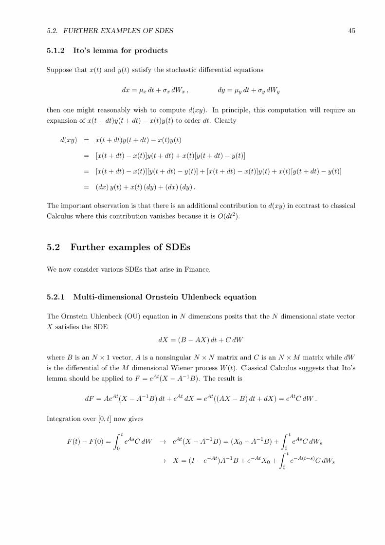
5.2. FURTHER EXAMPLES OF SDES 45
5.1.2 Ito’s lemma for products
Suppose that x(t) and y(t) satisfy the stochastic differential equations
dx = µx dt+ σx dWx , dy = µy dt+ σy dWy
then one might reasonably wish to compute d(xy). In principle, this computation will require an
expansion of x(t+ dt)y(t+ dt)− x(t)y(t) to order dt. Clearly
d(xy) = x(t+ dt)y(t+ dt)− x(t)y(t)
= [x(t+ dt)− x(t)]y(t+ dt) + x(t)[y(t+ dt)− y(t)]
= [x(t+ dt)− x(t)][y(t+ dt)− y(t)] + [x(t+ dt)− x(t)]y(t) + x(t)[y(t+ dt)− y(t)]
= (dx) y(t) + x(t) (dy) + (dx) (dy) .
The important observation is that there is an additional contribution to d(xy) in contrast to classical
Calculus where this contribution vanishes because it is O(dt2).
5.2 Further examples of SDEs
We now consider various SDEs that arise in Finance.
5.2.1 Multi-dimensional Ornstein Uhlenbeck equation
The Ornstein Uhlenbeck (OU) equation in N dimensions posits that the N dimensional state vector
X satisfies the SDE
dX = (B −AX) dt+ C dW
where B is an N × 1 vector, A is a nonsingular N ×N matrix and C is an N ×M matrix while dW
is the differential of the M dimensional Wiener process W (t). Classical Calculus suggests that Ito’s
lemma should be applied to F = eAt(X −A−1B). The result is
dF = AeAt(X −A−1B) dt+ eAt dX = eAt((AX −B) dt+ dX) = eAtC dW .
Integration over [0, t] now gives
F (t)− F (0) =
∫ t
0eAsC dW → eAt(X −A−1B) = (X0 −A−1B) +
∫ t
0eAsC dWs
→ X = (I − e−At)A−1B + e−AtX0 +
∫ t
0e−A(t−s)C dWs
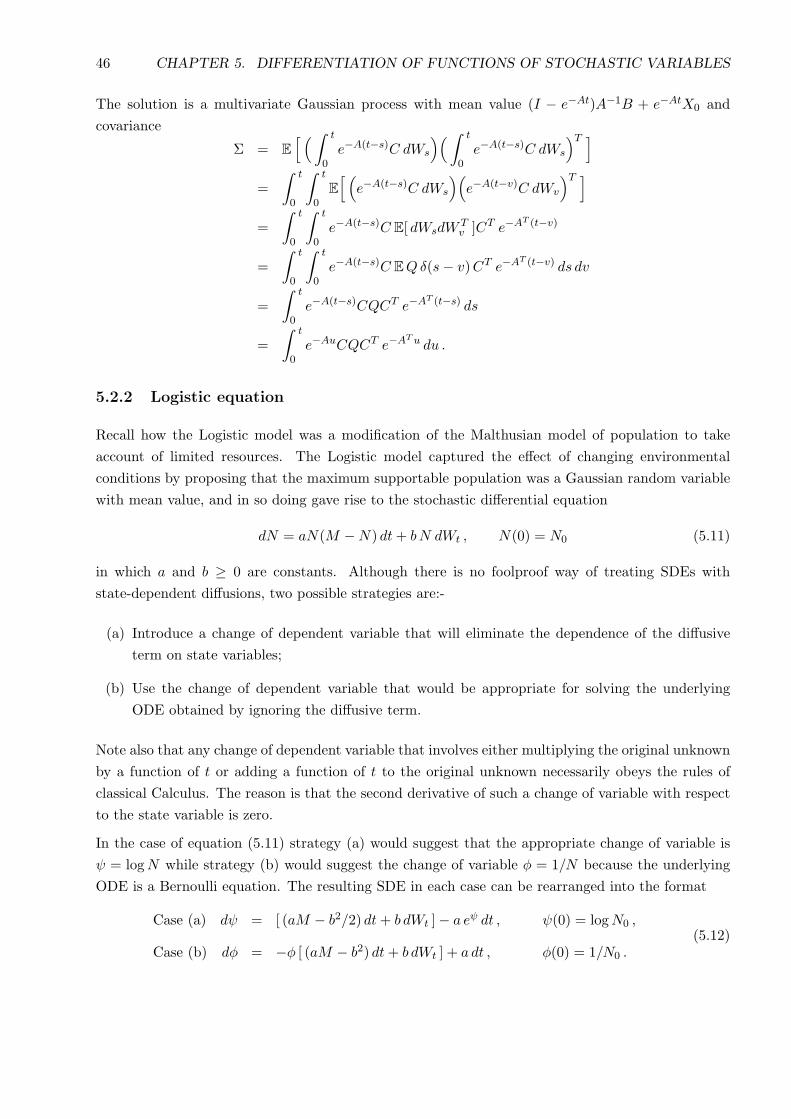
46 CHAPTER 5. DIFFERENTIATION OF FUNCTIONS OF STOCHASTIC VARIABLES
The solution is a multivariate Gaussian process with mean value (I − e−At)A−1B + e−AtX0 and
covariance
Σ = E[ ( ∫ t
0e−A(t−s)C dWs
)(∫ t
0e−A(t−s)C dWs
)T ]=
∫ t
0
∫ t
0E[ (e−A(t−s)C dWs
)(e−A(t−v)C dWv
)T ]=
∫ t
0
∫ t
0e−A(t−s)C E[ dWsdW
Tv ]CT e−A
T (t−v)
=
∫ t
0
∫ t
0e−A(t−s)C EQδ(s− v)CT e−A
T (t−v) ds dv
=
∫ t
0e−A(t−s)CQCT e−A
T (t−s) ds
=
∫ t
0e−AuCQCT e−A
Tu du .
5.2.2 Logistic equation
Recall how the Logistic model was a modification of the Malthusian model of population to take
account of limited resources. The Logistic model captured the effect of changing environmental
conditions by proposing that the maximum supportable population was a Gaussian random variable
with mean value, and in so doing gave rise to the stochastic differential equation
dN = aN(M −N) dt+ bN dWt , N(0) = N0 (5.11)
in which a and b ≥ 0 are constants. Although there is no foolproof way of treating SDEs with
state-dependent diffusions, two possible strategies are:-
(a) Introduce a change of dependent variable that will eliminate the dependence of the diffusive
term on state variables;
(b) Use the change of dependent variable that would be appropriate for solving the underlying
ODE obtained by ignoring the diffusive term.
Note also that any change of dependent variable that involves either multiplying the original unknown
by a function of t or adding a function of t to the original unknown necessarily obeys the rules of
classical Calculus. The reason is that the second derivative of such a change of variable with respect
to the state variable is zero.
In the case of equation (5.11) strategy (a) would suggest that the appropriate change of variable is
ψ = logN while strategy (b) would suggest the change of variable ϕ = 1/N because the underlying
ODE is a Bernoulli equation. The resulting SDE in each case can be rearranged into the format
Case (a) dψ = [ (aM − b2/2) dt+ b dWt ]− a eψ dt , ψ(0) = logN0 ,
Case (b) dϕ = −ϕ [ (aM − b2) dt+ b dWt ] + a dt , ϕ(0) = 1/N0 .(5.12)
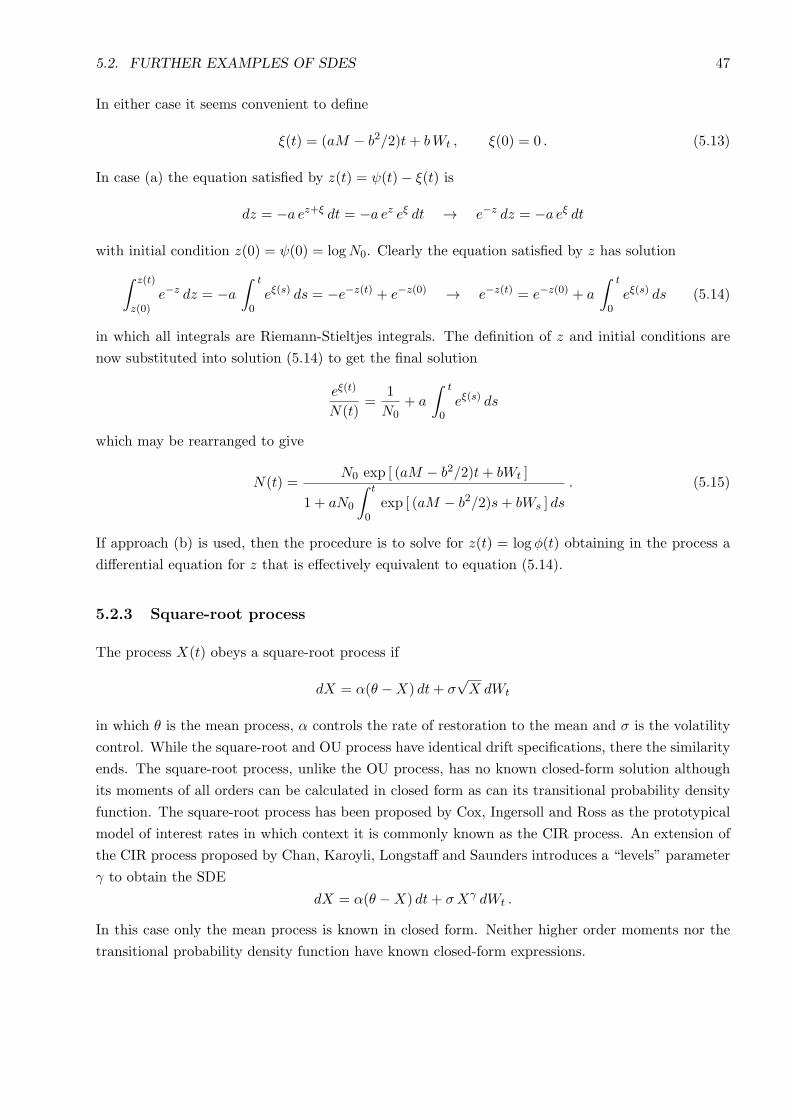
5.2. FURTHER EXAMPLES OF SDES 47
In either case it seems convenient to define
ξ(t) = (aM − b2/2)t+ bWt , ξ(0) = 0 . (5.13)
In case (a) the equation satisfied by z(t) = ψ(t)− ξ(t) is
dz = −a ez+ξ dt = −a ez eξ dt → e−z dz = −a eξ dt
with initial condition z(0) = ψ(0) = logN0. Clearly the equation satisfied by z has solution∫ z(t)
z(0)e−z dz = −a
∫ t
0eξ(s) ds = −e−z(t) + e−z(0) → e−z(t) = e−z(0) + a
∫ t
0eξ(s) ds (5.14)
in which all integrals are Riemann-Stieltjes integrals. The definition of z and initial conditions are
now substituted into solution (5.14) to get the final solution
eξ(t)
N(t)=
1
N0+ a
∫ t
0eξ(s) ds
which may be rearranged to give
N(t) =N0 exp [ (aM − b2/2)t+ bWt ]
1 + aN0
∫ t
0exp [ (aM − b2/2)s+ bWs ] ds
. (5.15)
If approach (b) is used, then the procedure is to solve for z(t) = log ϕ(t) obtaining in the process a
differential equation for z that is effectively equivalent to equation (5.14).
5.2.3 Square-root process
The process X(t) obeys a square-root process if
dX = α(θ −X) dt+ σ√X dWt
in which θ is the mean process, α controls the rate of restoration to the mean and σ is the volatility
control. While the square-root and OU process have identical drift specifications, there the similarity
ends. The square-root process, unlike the OU process, has no known closed-form solution although
its moments of all orders can be calculated in closed form as can its transitional probability density
function. The square-root process has been proposed by Cox, Ingersoll and Ross as the prototypical
model of interest rates in which context it is commonly known as the CIR process. An extension of
the CIR process proposed by Chan, Karoyli, Longstaff and Saunders introduces a “levels” parameter
γ to obtain the SDE
dX = α(θ −X) dt+ σXγ dWt .
In this case only the mean process is known in closed form. Neither higher order moments nor the
transitional probability density function have known closed-form expressions.
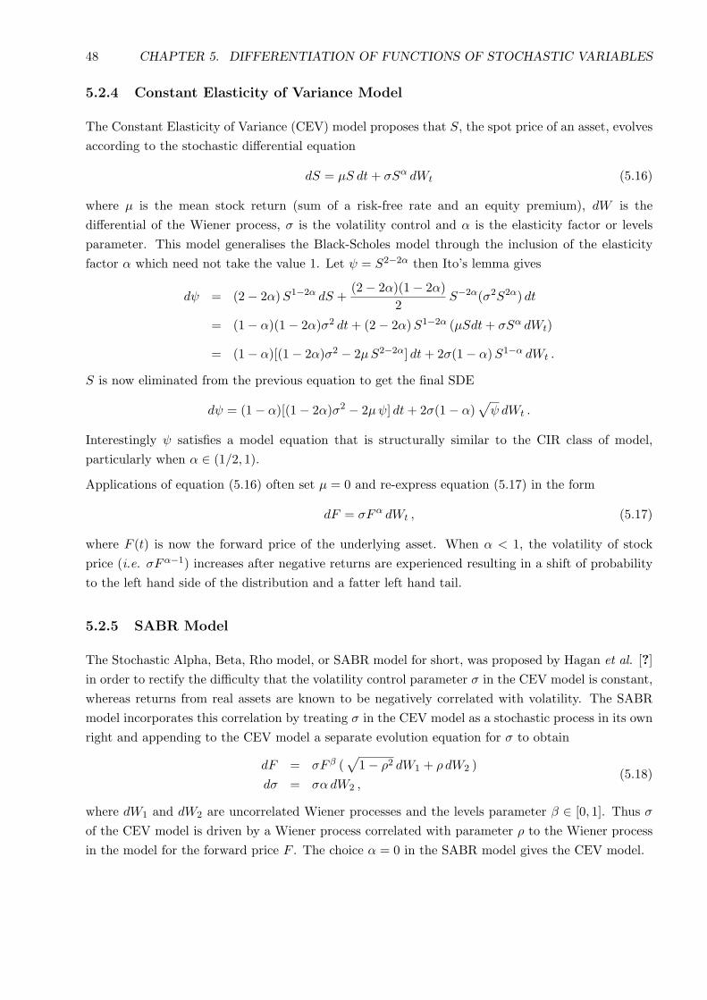
48 CHAPTER 5. DIFFERENTIATION OF FUNCTIONS OF STOCHASTIC VARIABLES
5.2.4 Constant Elasticity of Variance Model
The Constant Elasticity of Variance (CEV) model proposes that S, the spot price of an asset, evolves
according to the stochastic differential equation
dS = µS dt+ σSα dWt (5.16)
where µ is the mean stock return (sum of a risk-free rate and an equity premium), dW is the
differential of the Wiener process, σ is the volatility control and α is the elasticity factor or levels
parameter. This model generalises the Black-Scholes model through the inclusion of the elasticity
factor α which need not take the value 1. Let ψ = S2−2α then Ito’s lemma gives
dψ = (2− 2α)S1−2α dS +(2− 2α)(1− 2α)
2S−2α(σ2S2α) dt
= (1− α)(1− 2α)σ2 dt+ (2− 2α)S1−2α (µSdt+ σSα dWt)
= (1− α)[(1− 2α)σ2 − 2µS2−2α] dt+ 2σ(1− α)S1−α dWt .
S is now eliminated from the previous equation to get the final SDE
dψ = (1− α)[(1− 2α)σ2 − 2µψ] dt+ 2σ(1− α)√ψ dWt .
Interestingly ψ satisfies a model equation that is structurally similar to the CIR class of model,
particularly when α ∈ (1/2, 1).
Applications of equation (5.16) often set µ = 0 and re-express equation (5.17) in the form
dF = σFα dWt , (5.17)
where F (t) is now the forward price of the underlying asset. When α < 1, the volatility of stock
price (i.e. σFα−1) increases after negative returns are experienced resulting in a shift of probability
to the left hand side of the distribution and a fatter left hand tail.
5.2.5 SABR Model
The Stochastic Alpha, Beta, Rho model, or SABR model for short, was proposed by Hagan et al. [?]
in order to rectify the difficulty that the volatility control parameter σ in the CEV model is constant,
whereas returns from real assets are known to be negatively correlated with volatility. The SABR
model incorporates this correlation by treating σ in the CEV model as a stochastic process in its own
right and appending to the CEV model a separate evolution equation for σ to obtain
dF = σF β (√
1− ρ2 dW1 + ρ dW2 )
dσ = σα dW2 ,(5.18)
where dW1 and dW2 are uncorrelated Wiener processes and the levels parameter β ∈ [0, 1]. Thus σ
of the CEV model is driven by a Wiener process correlated with parameter ρ to the Wiener process
in the model for the forward price F . The choice α = 0 in the SABR model gives the CEV model.
5.3. HESTON’S MODEL 49
The volatility in the SABR model follows a geometric walk with zero drift and solution
σ(t) = σ0 exp(− α2t
2+ αW2(t)
),
where σ0 is the initial value of σ. Despite the closed-form expression for σ(t) the SABR model has no
closed-form solutions except in the cases β = 0 (solve for F ) and β = 1 (solve for logF ). In overview,
the values of the parameters ρ and β control the curvature of the volatility smile whereas the value
of α, the volatility of volatility, controls the skewness of the lognormal distribution of volatility.
5.3 Heston’s Model
The SABR model is a recent example of a stochastic volatility options pricing model of which there
exists many. The most renowned and widely used of these is Heston’s model. The model was proposed
in 1993 and when reformulated in terms of y = logS posits that
dy = (r + β h) dt+√h (ρ dWt +
√1− ρ2 dZt) ,
dh = κ(γ − h) dt+ σ√h dWt ,
(5.19)
where h is volatility and dWt and dZt are increments in the independent Wiener processes Wt and
Zt, the parameter β = λ(1−ρ2)−1/2 contains the equity premium, r is the risk-free force of interest
and ρ ∈ [−1, 1] is the correlation between innovations in asset returns and volatility.
However, Heston’s model is an example of a bivariate affine process. While the transitional probability
density function cannot be computed in closed form, it is possible to determine the characteristic
function of Heston’s model in closed form. This calculation requires the solution of partial differential
equations and will be the focus of our attention in a later chapter.
5.4 Girsanov’s lemma
Girsanov’s lemma is concerned with changes of measure and the Radon-Nikodym2 derivative. A
simple way to appreciate what is meant by a change in measure is to consider the evolution of asset
prices as described by a binomial with transitions of fixed duration. Suppose the spot price of an
asset is S, and that at the next transition the price of the asset is either Su (> S) with probability
q or Sd (< S) with probability (1 − q), and take Q to be the measure under which the expected
one-step-ahead asset price is S, i.e. the process is a Q-Martingale. Clearly the value of q satisfies
Suq + Sd(1− q) = S → q =S − SdSu − Sd
leading to upward and downward movements of the asset price with respective probabilities
q =S − SdSu − Sd
, 1− q =Su − S
Su − Sd.
2The Radon-Nikodym derivative is essentially a Jacobian.
50 CHAPTER 5. DIFFERENTIATION OF FUNCTIONS OF STOCHASTIC VARIABLES
Let P be another measure in which the asset price at each transition moves upwards with probability
p and downwards with probability (1−p) and consider a pathway (or filtration) through the binomial
tree consisting of N transitions in which the asset price moved upwards n times and downwards N−ntimes attaining the sequence of states S1, S2, · · · , SN . The likelihoods associated with this path under
the P and Q measures are respectively
L(P )(S1, · · · , SN ) = pn(1− p)N−n , L(Q)(S1, · · · , SN ) = qn(1− q)N−n .
The likelihood ratio of the Q measure to the P measure is therefore
LN (S1, · · · , SN ) =qn(1− q)N−n
pn(1− p)N−n =(qp
)n(1− q
1− p
)N−n.
Clearly the value of LN is a function of the path (or filtration - say FN ) - straightforward in this case
because it is only the number of upward and downward movements that matter and not when these
movements occur. The quantity LN is called the “Radon-Nikodym” derivative of Q with respect to
P and is commonly written
LN =dQdP
∣∣∣∣FN
.
Moreover
LN+1
LN=
q
pSN+1 > SN ,
1− q
1− pSN+1 < SN .
The expectation of LN+1 under the P measure conditional on the filtration FN gives
EP[LN+1 | FN ] = p(LN × q
p
)+ (1− p)
(LN × 1− q
1− p
)= LN .
Thus LN , or in general the Radon-Nikodym derivative, is a martingale with respect to the P measure.
But L0 = 1 and so iteration of the identity EP[LN+1 | FN ] = LN indicates that EP[LN ] = 1. In this
illustration we associate the P measures with risk in our (risk-averse) world and for this reason
it is usually called the “Physical” measure. By contrast, the measure Q is commonly called the
“Risk-Neutral” measure.
Now consider EP[ψ LN | FN ]. The value is
ψU
(qpLN
)p+ ψD
(1− q
1− pLN
)(1− p) = (ψU q + ψD (1− q))LN = EQ[ψ | FN ]
and so the Radon-Nikodym derivative enjoys the key property that it allows expectations with respect
to the Q measure to be expressed as expectations with respect to the P via the formula
EQ [ Ψ ] = EP [ ΨLN ]
where Ψ, for example, is the payoff from a call option.
5.4. GIRSANOV’S LEMMA 51
5.4.1 Change of measure for a Wiener process
The illustrative example involving the binomial tree expressed changes in measure in terms of re-
weighting the probability of upward and downward movement, and in so doing the probabilities
associated with pathways through the tree. The same procedure can be extended to continuous
processes, and in particular the Wiener process. The natural measure P on the Wiener process is
associated with the probability density function
p(x) =1√2π
exp[− x2
2
].
Suppose, for example, that the Wiener process W (t) attains the values (x1, . . . , xn) at the respective
times (t1, . . . , tn) in which D = t0, · · · , tn is a dissection of the finite interval [0, T ]. Because
increments of W (t) are independent, then the likelihood L(n)(P ) associated with this path is
L(P )(x1, · · · , xn) =n∏i=1
1√2π∆ti
exp
(−(∆xi)
2
2∆ti
),
where ∆xi = xi − xi−1 and ∆ti = ti − ti−1. The limit of this expression may be interpreted as the
measure P for the continuous process W (t). The question is now to determine how W (t) changes
under a different measure, say Q, and of course what restrictions (if any) must be imposed on Q.
Equivalent measure
Equivalence in the case of the binomial tree is the condition p > 0 ⇐⇒ q > 0. In effect, the
measures P and Q must both refer to binomial trees and not a binomial tree in one measure and a
cascading process in the other measure. Equivalence between the measures P and Q in the binomial
tree is a particular instance of the following definition of equivalence.
Two measures P and Q are equivalent (i.e. one can be distorted into the other) if and only if the
measures agree on which events have zero probability, i.e.
P(X) > 0 ⇐⇒ Q(X) > 0 .
Given two equivalent measures P and Q, the “Radon-Nikodym” derivative of Q with respect to P is
defined by the likelihood ratio
dQdP
= limn→∞
L(Q)(x1, · · · , xn)L(P )(x1, · · · , xn)
.
Alternatively one may write
Q(X) =
∫XdQ(x) =
∫XϕdP(x)
where ϕ = dQ/dP is the Radon-Nikodym derivative of Q with respect to P. Clearly ϕ simply states
what distortion should be applied to the measure P to get the measure Q. Given and function Ψ,
then
EQ [Ψ ] = EP [Ψϕ ] .
52 CHAPTER 5. DIFFERENTIATION OF FUNCTIONS OF STOCHASTIC VARIABLES
5.4.2 Girsanov theorem
Let W (t) be a P-Wiener process under the natural filtration Ft, namely that for which the probabil-
ities of paths are determined directly from the N(0, 1) probability density function, and define Z(t)
to be a process adapted from W (t) for which Novikov’s condition
E[exp
(12
∫ T
0Z2(s) ds
) ]<∞
is satisfied for some finite time horizon T . Let Q to be a measure related to P with Radon-Nikodym
derivative
ϕ(t) =dQdP
= exp(−
∫ t
0Z(s) dW (s)− 1
2
∫ t
0Z2(s) ds
).
Under the probability measure Q, the process
W (ϕ)(t) =W (t) +
∫ t
0Z(s) ds
is a standard Wiener process.
Justification
From the definition of Q it is clear that P and Q are equivalent measures. One strategy is use the
moment generating function to demonstrate that W (ϕ)(t) is a natural Wiener process under the Qmeasure, namely that EQ [W (ϕ)(t) ] = 0 and that VQ [W (ϕ)(t) ] = t. We begin by recalling that the
moment generating function of the Gaussian distribution N(µ, σ2) is
M(θ) = EP[ e θX ] =1√2π σ
∫ReθXe−(X−µ)2/2σ2
dX = e θµ+θ2σ2/2 .
The formal proof of Girsanov’s theorem starts with the Radon-Nikodym identity
EQ [Ψ ] = EP[ dQdP
Ψ]
when particularized by replacing Ψ with e θW(ϕ)(t) to get
EQ [ e θW(ϕ)(t) ] = EP
[ dQdP
e θW(ϕ)(t)
]= EP
[exp
(−
∫ t
0Z(s) dW (s)− 1
2
∫ t
0Z2(s) ds
)exp
(θW (t) + θ
∫ t
0Z(s) ds
) ]= exp
(θ
∫ t
0Z(s) ds− 1
2
∫ t
0Z2(s) ds
)EP
[exp
(θW (t)−
∫ t
0Z(s) dW (s)
) ]
The focus is now on the computation of EP[exp
(θW (t)−
∫ t0 Z(s) dW (s)
) ]. For convenience let
ξ(t) = θW (t)−∫ t
0Z(s) dW (s)
5.4. GIRSANOV’S LEMMA 53
then EP[ ξ(t) ] = 0 and
VP[ ξ(t) ] = EP[ θ2W 2(t) ]− 2θEP[W (t)
∫ t
0Z(s) dW (s)
]+ EP
[ ( ∫ t
0Z(s) dW (s)
)2 ]= θ2 t− 2θ
∫ t
0Z(s)EP [W (t) dW (s) ] +
∫ t
0Z2(s) ds
Clearly the Novikov condition simply guarantees that e ξ(t) has finite mean and variance. Moreover,
it is obvious that EP [W (t) dW (s) ] = ds and therefore
EP[ ξ(t) ] = 0 ,
VP[ ξ(t) ] = θ2 t− 2θ
∫ t
0Z(s) ds+
∫ t
0Z2(s) ds .
It now follows from the moment generating function of N(µ, σ2) with µ = 0 and θ = 1 that
EP[ e ξ(t) ] = exp(θ22t− θ
∫ t
0Z(s) ds+
1
2
∫ t
0Z2(s) ds
).
Consequently
EQ [ e θW(ϕ)(t) ] = exp
(θ
∫ t
0Z(s) ds− 1
2
∫ t
0Z2(s) ds
)EP
[exp
(θW (t)−
∫ t
0Z(s) dW (s)
)= exp
(θ
∫ t
0Z(s) ds− 1
2
∫ t
0Z2(s) ds
)exp
(θ22t− θ
∫ t
0Z(s) ds+
1
2
∫ t
0Z2(s) ds
)= exp
(θ22t).
which is just the moment generating function of a standard Wiener process, thereby establish the
claim of the Girsanov’s theorem.

54 CHAPTER 5. DIFFERENTIATION OF FUNCTIONS OF STOCHASTIC VARIABLES
Chapter 6
The Chapman Kolmogorov Equation
6.1 Introduction
Let the state of a system at time t after initialisation be described by the n-dimensional random
variable x(t) with sample space Ω. Let x1,x2, · · · be the measured state of the system at times
t1 > t2 > · · · ≥ 0, then x(t) is a stochastic process provided the joint probability density function
f(x1, t1;x2, t2; · · · ) (6.1)
exists for all possible sequences of measurements xk and times tk. When the joint probability density
function (6.1) exists, it can be used to construct the conditional probability density function
f(x1, t1;x2, t2; · · · |y1, τ1;y2, τ2; · · · ) (6.2)
which describes the likelihood of measuring x1,x2, · · · at times t1 > t2 > · · · ≥ 0, given that the
system attained the states y1,y2, · · · at times τ1 > τ2 > · · · ≥ 0 where, of necessity, t1 > t2 > · · · >τ1 > τ2 > · · · ≥ 0. Kolmogorov’s axioms of probability yield
f(x1, t1;x2, t2; · · · |y1, τ1;y2, τ2; · · · ) =f(x1, t1;x2, t2; · · · ;y1, τ1;y2, τ2; · · · )
f(y1, τ1;y2, τ2; · · · ), (6.3)
i.e. the conditional density is the usual ratio of the joint density of x and y (numerator) and the
marginal density of y (denominator). In the same notation there is a hierarchy of identities which
must be satisfied by the conditional probability density functions of any stochastic process. The first
identity is
f(x1, t1 ) =
∫Ωf(x1, t1;x, t ) dx =
∫Ωf(x1, t1 |x, t) f(x, t ) dx (6.4)
which apportions the probability with which the state x1 at future time t1 is accessed at a previous
time t from each x ∈ Ω. The second group of conditions take the generic form
f(x1, t1 |x2, t2; · · · ) =
∫Ωf(x1, t1;x, t; x2, t2; · · · ) dx
=
∫Ωf(x1, t1 |x, t; x2, t2; · · · ) f(x, t |x2, t2; · · · ) dx
(6.5)
55
56 CHAPTER 6. THE CHAPMAN KOLMOGOROV EQUATION
in which it is taken for granted that t1 > t > t2 > · · · ≥ 0. Similarly, a third group of conditions can
be constructed from identities (6.4) and (6.5) by regarding the pair (x1, t1) as a token and replacing
it with an arbitrary sequence of pairs involving the attainment of states at times after t.
Of course, equations (6.1-6.5) are also valid when Ω is a discrete sample space in which case the
joint probability density functions are sums of delta functions and integrals over Ω are replaced by
summations over Ω.
As might be anticipated the structure presented in equations (6.1-6.5) is too general for making
useful progress, and so it is desirable to introduce further simplifying assumptions. Two obvious
simplifications are possible.
(a) Assume that (xk, tk) are independent random variables. The joint probability density function
is therefore the product of the individual probabilities f(xk, tk), i.e.
f(x1, t1;x2, t2; · · · |y1, τ1;y2, τ2; · · · ) = f(x1, t1;x2, t2; · · · ) =∏
f(xk, tk) .
In effect, there is no conditioning whatsoever in the resulting stochastic process and conse-
quently historical states contain no useful information.
(b) Assume that the current state perfectly captures all historical information. This is the simplest
paradigm to incorporate historical information within a stochastic process. Processes with this
property are called Markov processes.
Assumption (a) is too strong. It is taken “as read” that in practice it is observations of historical
states of a system in combination with time that conditions the distribution of future states, and not
just time itself as would be the case if assumption (a) is adopted.
6.1.1 Markov process
A stochastic process possesses the Markov property if the historical information in the process is
perfectly captured by the most recent observation of the process. In effect,
f(x1, t1;x2, t2; · · · |y1, τ1;y2, τ2; · · · ) = f(x1, t1;x2, t2; · · · |y1, τ1) (6.6)
where it is again assumed that t1 > t2 > · · · > τ1 > τ2 > · · · ≥ 0. Suppose that the sequence of states
under discussion are (xk, tk) where k = 1, · · · ,m then it follows directly from equation (6.3) that
f(x1, t1;x2, t2; · · · ;xm, tm ) = f(x1, t1; |x2, t2; · · · xm, tm ) f(x2, t2; · · · ; xm, tm ) (6.7)
and from equation (6.6) that
f(x1, t1 |x2, t2; · · · xm, tm ) = f(x1, t1 |x2, t2 ) . (6.8)
Consequently, for a Markov process, results (6.7) and (6.8) may be combined to give
f(x1, t1;x2, t2; · · · ;xm, tm ) = f(x1, t1 |x2, t2 ) f(x2, t2; · · · ; xm, tm ) . (6.9)
6.2. CHAPMAN-KOLMOGOROV EQUATION 57
Equation (6.9) forms the basis of an induction procedure from which it is follows directly that
f(x1, t1;x2, t2; · · · ;xm, tm ) = f(xm, tm )k=m−1∏k=1
f(xk, tk |xk+1, tk+1 ) . (6.10)
6.2 Chapman-Kolmogorov equation
Henceforth the stochastic process will be assumed to possess the Markov property. Identity (6.4)
remains unchanged. However, the identities characterised by equation (6.5) are now simplified since
the Markov property requires that
f(x1, t1 |x, t; x2, t2; · · · ) = f(x1, t1 |x, t ) ,
f(x, t |x2, t2; · · · ) = f(x, t |x2, t2 ) .
Consequently, the general condition (6.5) simplifies to
f(x1, t1 |x2, t2; · · · ) =∫Ωf(x1, t1 |x, t ) f(x, t |x2, t2 ) dx = f(x1, t1 |x2, t2 ) (6.11)
for Markov stochastic processes. This identity is called the Chapman-Kolmogorov equation. Further-
more, the distinction between the second and third groups of identities vanishes for Markov stochastic
processes.
Summary The probability density function f(x1, t1 ) and the conditional proba-
bility density function f(x1, t1 |x, t ) (often called the transitional probability density
function) for a Markov stochastic process satisfy the identities
f(x1, t1 ) =
∫Ωf(x1, t1 |x, t) f(x, t ) dx ,
f(x1, t1 |x2, t2 ) =
∫Ωf(x1, t1 |x, t ) f(x, t |x2, t2 ) dx .
In these identities time is regarded as a parameter which can be either discrete or
continuous.
When time is a continuous parameter the integral form of the Chapman-Kolmogorov property can
be expressed as a partial differential equation under relatively weak conditions. The continuity of the
process path with respect to time now becomes an issue to be addressed. The requirement of path
continuity imposes restrictions on the form of the transitional density function f(x1, t1 |x2, t2 ).
6.2.1 Path continuity
Suppose that a stochastic process starts at (y, t) and passes through (x, t+h). For a Markov process,
the distribution of possible states x is perfectly captured by the transitional probability density
58 CHAPTER 6. THE CHAPMAN KOLMOGOROV EQUATION
function f(x, t+ h |y, t ) where h ≥ 0. Given ε > 0, the probability that a path is more distant than
ε from y is just ∫|x−y|>ε
f(x, t+ h |y, t) dx . (6.12)
A process is said to be path-continuous if for any ε > 0∫|x−y|>ε
f(x, t+ h |y, t) dx = o(h) (6.13)
with probability one, and uniformly with respect to t, h and the state y. In effect, the probability
that a finite fraction of paths extend more than ε from y shrinks to zero faster than h. The concept
of path-continuity is often captured by the definition
Path-Continuity Given any x,y ∈ Ω satisfying |x− y| > ε and t > 0, assume
that the limit
limh→0+
f(x, t+ h |y, t)h
= ϕ(x |y, t )
exists and is uniform with respect to x, y and t.
Path-continuity is characterised by the property ϕ(x |y, t ) = 0 when x = y.
Example
Investigate the path continuity of the one dimensional Markov processes defined by the transitional
density functions
(a) f(x, t+ h | y, t) = 1√2π h
e−(x−y)2/2h2 , (b) f(x, t+ h | y, t) = h
π
1
h2 + (x− y)2.
Solution
It is demonstrated easily that both expressions are non-negative and integrate to unity with respect
to x for any t, h and y. Each expression therefore defines a valid transitional density function. Note,
in particular, that both densities satisfy automatically the consistency condition
limh→0+
f(x, t+ h |y, t) = δ(x− y) .
Density (a) Consider∫|x−y|>ε
f(x, t+ h | y, t) dx =
∫ ∞
y+ε
1√2π h
e−(x−y)2/2h2 dx+
∫ y−ε
−∞
1√2π h
e−(x−y)2/2h2 dx
=2√2π h
∫ ∞
εe−x
2/2h2 dx
=1√π
∫ ∞
ε2/2h2y−1/2 e−y dy
6.2. CHAPMAN-KOLMOGOROV EQUATION 59
Since y ≥ ε2/2h2 in this integral then y−1/2 ≤√2 (h/ε). Thus
1
h
∫|x−y|>ε
f(x, t+ h | y, t) dx <√
2
π
1
ε
∫ ∞
ε2/2h2e−y dy =
√2
π
1
ε
[1− e−ε
2/2h2]→ 0
as h → 0+, and therefore the stochastic process defined by the transitional probability density
function (a) is path-continuous.
Density (b) Consider∫|x−y|>ε
f(x, t+ h | y, t) dx =
∫ ∞
y+ε
h
π
dx
h2 + (x− y)2+
∫ y−ε
−∞
h
π
dx
h2 + (x− y)2
=2h
π
∫ ∞
ε
dx
h2 + x2
=2
π
[tan−1 x
h
]∞ε
=2
π
[ π2− tan−1 ε
h
].
For fixed ε > 0, define h = ε tan θ so that the limiting process h → 0+ may be replaced by the
limiting process θ → 0+. Thus
1
h
∫|x−y|>ε
f(x, t+ h | y, t) dx =2θ
πε tan θ→ 2
πε= 0
as h → 0+, and therefore the stochastic process defined by the transitional probability density
function (b) is not path-continuous.
Remarks
The transitional density function (a) describes a Brownian stochastic process. Consequently, a Brow-
nian path is continuous although it has no well-defined velocity. The transitional density function (b)
describes a Cauchy stochastic process which, by comparison with the Brownian stochastic process,
is seen to be discontinuous.
6.2.2 Drift and diffusion
Suppose that for a particular stochastic process the change of state in moving from y to x, i.e.
(x − y), occurs during the time interval [t, t + h] with probability f(x, t + h |y, t ). The drift and
diffusion of this process characterise respectively the expected rate of change in state, calculated over
all paths terminating within distance ε of y, and the rate of generation of the covariance of these
changes. The drift and diffusion are defined as follows.
60 CHAPTER 6. THE CHAPMAN KOLMOGOROV EQUATION
Drift The drift of a (Markov) process at y is defined to be the instantaneous rate of
change of state for all processes close to y and is the value of the limit
limε→0+
[limh→0+
1
h
∫|x−y|<ε
(x− y ) f(x, t+ h |y, t) dx]= a(y, t) , (6.14)
which is assumed to exist, and which requires that the inner limit converges uniformly with
respect to y, t and ε.
Diffusion The instantaneous covariance of a (Markov) process at y is defined to be the
instantaneous rate of change of covariance for all processes close to y and is the value of
the limit
limε→0+
[limh→0+
1
h
∫|x−y|<ε
(x− y )⊕ (x− y ) f(x, t+ h |y, t) dx]= g(y, t) , (6.15)
which is assumed to exist, and which requires that the inner limit converges uniformly with
respect to y, t and ε.
Finally, all third and higher order moments computed over states x,y ∈ Ω satisfying |x − y| > ε
necessarily vanish as ε→ 0+ because the integral defining the k-th moment is O(εk−2) for k ≥ 2.
6.2.3 Drift and diffusion of an SDE
Suppose that the time course of the process x(t) = x1(t), · · · , xN (t) follows the stochastic differentialequation
dxj = µj(x, t) dt+
M∑α=1
σjα(x, t) dWα (6.16)
where 1 ≤ j ≤ N and dW1, · · · , dWM are increments in the correlatedM Wiener processesW1, · · · ,WM
such that EP [ dWj dWk ] = Qjk dt. The issue is now to use the general definition of drift and diffusion
to determine the drift and diffusion specifications in the case of the SDE 6.16.
The expected drift at x during [t, t+ h] is
aj = limh→0+
1
hE [ dxj ] = lim
h→0+
1
hE[µj(x, t)h+
M∑α=1
σjα(x, t) dWα
]= lim
h→0+
1
hE [µj(x, t)h ] = µj(x, t) .
(6.17)
6.3. FORMAL DERIVATION OF THE FORWARD KOLMOGOROV EQUATION 61
The expected covariance at x during [t, t+ h] is
gjk = limh→0+
1
hE [ (dxj − µj h)((dxj − µj h) ]
= limh→0+
1
h
M∑α,β=1
E [σjα dWα σkβ dWβ ]
= limh→0+
M∑α,β=1
σjα σkβh
E [ dWα dWβ ] =M∑
α,β=1
σjαQαβ σkβ .
(6.18)
Evidently gjk is a symmetric array. Furthermore, since Q is positive definite then Q = FTF and
ΣQΣT = ΣFT FΣT = (F ΣT)T (FΣT) and therefore G = [gjk] is also positive definite, as required.
6.3 Formal derivation of the Forward Kolmogorov Equation
The construction of the differential equation representation of the Chapman-Kolmogorov condition
follows closely the discussion of path-continuity, but admits the possibility of discontinuous paths by
extending the analysis to include Markov processes for which
∫|x−y|>ε
f(x, t+ h |y, t) dx = O(h) (6.19)
as h → 0+. The Cauchy stochastic process gives an example of a qualifying transitional probability
density function. Suppose that ε > 0 is given together with a Markov process with transitional
probability density function f(x1, t1 |x2, t2 ).
Let ψ(x) be an arbitrary twice continuously differentiable function of state, then the rate of change
of the expected value of ψ is defined by
∂
∂t
∫Ωψ(x) f(x, t |y, T ) dx = lim
h→0+
1
h
[ ∫Ωψ(x) [ f(x, t+ h |y, T )− f(x, t |y, T ) ] dx
]= lim
h→0+
1
h
[ ∫Ωψ(x)
( ∫Ωf(x, t+ h | z, t) f(z, t |y, T ) dz
)dx
−∫Ωψ(z) f(z, t |y, T ) dz
]= lim
h→0+
1
h
[ ∫Ω
∫Ωψ(x)f(z, t |y, T ) f(x, t+ h | z, t) dx dz
−∫Ωψ(z) f(z, t |y, T ) dz
](6.20)
where the Chapman-Kolmogorov property has been used on the first integral on the right hand side
of equation (6.20). The sample space Ω is now divided into the regions |x − z| < ε and |x − z| > ε
62 CHAPTER 6. THE CHAPMAN KOLMOGOROV EQUATION
where ε is sufficiently small that ψ(x) may be represented by the Taylor series expansion
ψ(x) = ψ(z) +N∑k=1
(xk − zk)∂ψ(z)
∂ zk+
1
2
N∑j,k=1
(xj − zj ) (xk − zk)∂2ψ(z)
∂ zj ∂ zk
+
N∑j,k=1
(xj − zj)(xk − zk)Rjk(x, z)
(6.21)
within the region |x − z| < ε and in which Rjk(x, z) → 0 as |x − z| → 0. The right hand side of
equation (6.21) is now manipulated through a number of steps after first replacing ψ(x) by its Taylor
series and rearranging expression
limh→0+
1
h
[ ∫Ω
∫Ωψ(x)f(z, t |y, T ) f(x, t+ h | z, t) dx dz−
∫Ωψ(z) f(z, t |y, T ) dz
](6.22)
by means of the decomposition
limε→0+
[limh→0+
1
h
∫Ω
∫|x−z|<ε
ψ(x) f(z, t |y, T ) f(x, t+ h | z, t) dx dz
+ limh→0+
1
h
∫Ω
∫|x−z|>ε
ψ(x) f(z, t |y, T ) f(x, t+ h | z, t) dx dz
− limh→0+
1
h
∫Ωψ(z) f(z, t |y, T ) dz
].
(6.23)
Substituting the Taylor series for ψ(x) into expression (6.23) gives
limε→0+
limh→0+
1
h
[ ∫Ω
∫|x−z|<ε
ψ(z) f(z, t |y, T ) f(x, t+ h | z, t) dx dz
+
∫Ω
∫|x−z|<ε
(xk − zk)∂ψ(z)
∂ zkf(z, t |y, T ) f(x, t+ h | z, t) dx dz
+1
2
N∑j,k=1
∫Ω
∫|x−z|<ε
(xj − zj)(xk − zk)∂2ψ(z)
∂ zj ∂ zkf(z, t |y, T ) f(x, t+ h | z, t) dx dz
+
N∑j,k=1
∫Ω
∫|x−z|<ε
(xj − zj)(xk − zk)Rjk(x, z) f(z, t |y, T ) f(x, t+ h | z, t) dx dz
+
∫Ω
∫|x−z|>ε
ψ(x) f(z, t |y, T ) f(x, t+ h | z, t) dx dz−∫Ωψ(z) f(z, t |y, T ) dz
].
(6.24)
The definition of instantaneous drift in formula (6.14) is now used to deduce that
limε→0+
limh→0+
1
h
N∑k=1
∫Ω
∫|x−z|<ε
(xk − zk)∂ψ(z)
∂ zkf(z, t |y, T ) f(x, t+ h | z, t) dx dz
=
N∑k=1
∫Ωak(z, t)
∂ψ(z)
∂ zkf(z, t |y, T ) dz .
(6.25)
Similarly, the definition of instantaneous covariance in formula (6.15) is used to deduce that
limε→0+
limh→0+
1
2h
N∑j,k=1
∫Ω
∫|x−z|<ε
(xj − zj)(xk − zk)∂2ψ(z)
∂ zj ∂ zkf(z, t |y, T ) f(x, t+ h | z, t) dx dz
=1
2
N∑j,k=1
∫Ωgjk(z, t)
∂2ψ(z)
∂ zj ∂ zkf(z, t |y, T ) dz . (6.26)
6.3. FORMAL DERIVATION OF THE FORWARD KOLMOGOROV EQUATION 63
Moreover, since Rjk(x, z) → 0 as |x − z| → 0 then it is obvious that the contribution from the
remainder of the Taylor series becomes arbitrarily small as ε→ 0+ and therefore
limε→0+
limh→0+
1
h
N∑j,k=1
∫Ω
∫|x−z|<ε
(xj − zj)(xk − zk)Rjk(x, z) f(z, t |y, T ) f(x, t+ h | z, t) dx dz = 0 .
This result, together with (6.25) and (6.26) enable expression (6.24) to be further simplified to
limε→0+
limh→0+
1
h
[ ∫Ω
∫|x−z|<ε
ψ(z) f(z, t |y, T ) f(x, t+ h | z, t) dx dz
+
∫Ω
∫|x−z|>ε
ψ(x) f(z, t |y, T ) f(x, t+ h | z, t) dx dz−∫Ωϕ(z) f(z, t |y, T ) dz
]+
N∑k=1
∫Ωak(z, t)
∂ψ(z)
∂ zkf(z, t |y, T ) dz+ 1
2
N∑j,k=1
∫Ωgjk(z, t)
∂2ψ(z)
∂ zj ∂ zkf(z, t |y, T ) dz .
(6.27)
However, f(x, t+ h | z, t) is itself a probability density function and therefore satisfies∫Ωf(x, t+ h | z, t) dx = 1 .
Consequently, the first integral in expression (6.27) can be manipulated into the form∫Ω
∫|x−z|<ε
ψ(z) f(z, t |y, T ) f(x, t+ h | z, t) dx dz
=
∫Ωψ(z) f(z, t |y, T )
( ∫Ωf(x, t+ h | z, t) dx−
∫|x−z|>ε
f(x, t+ h | z, t) dx)dz
=
∫Ωψ(z) f(z, t |y, T ) dz−
∫Ω
∫|x−z|>ε
ψ(z) f(z, t |y, T ) f(x, t+ h | z, t) dx dz .
(6.28)
The first integral appearing in expression (6.27) is now replaced by equation (6.28). After some
obvious cancellation, the expression becomes
limε→0+
limh→0+
1
h
[ ∫Ω
∫|x−z|>ε
ψ(x) f(z, t |y, T ) f(x, t+ h | z, t) dx dz
−∫Ω
∫|x−z|>ε
ψ(z) f(z, t |y, T ) f(x, t+ h | z, t) dx dz]
+
N∑k=1
∫Ωak(z, t)
∂ψ(z)
∂ zkf(z, t |y, T ) dz+ 1
2
N∑j,k=1
∫Ωgjk(z, t)
∂2ψ(z)
∂ zj ∂ zkf(z, t |y, T ) dz .
(6.29)
The path-continuity condition (6.12) is now used to treat the limits in expression (6.29). Clearly
limε→0+
limh→0+
1
h
[ ∫Ω
∫|x−z|>ε
ψ(x) f(z, t |y, T ) f(x, t+ h | z, t) dx dz
−∫Ω
∫|x−z|>ε
ψ(z) f(z, t |y, T ) f(x, t+ h | z, t) dx dz]
=
∫Ω
∫Ωψ(x) f(z, t |y, T )ϕ(x, z) dx dz−
∫Ω
∫Ωψ(z) f(z, t |y, T )ϕ(x, z) dx dz
]=
∫Ω
∫Ωψ(z)
[f(x, t |y, T )ϕ(z,x)− f(z, t |y, T )ϕ(x, z)
]dx dz ,
(6.30)
64 CHAPTER 6. THE CHAPMAN KOLMOGOROV EQUATION
and consequently expression (6.24) is finally simplified to∫Ω
∫Ωψ(z)
[f(x, t |y, T )ϕ(z,x)− f(z, t |y, T )ϕ(x, z)
]dx dz
+
N∑k=1
∫Ωak(z, t)
∂ψ(z)
∂ zkf(z, t |y, T ) dz+ 1
2
N∑j,k=1
∫Ωgjk(z, t)
∂2ψ(z)
∂ zj ∂ zkf(z, t |y, T ) dz .
(6.31)
Expression (6.31) is now incorporated into equation (6.20) to obtain the final form
∫Ωψ(z)
∂ f(z, t |y, T )∂t
dz =
∫Ω
∫Ωψ(z)
[f(x, t |y, T )ϕ(z,x)− f(z, t |y, T )ϕ(x, z)
]dx dz
+N∑k=1
∫Ωak(z, t)
∂ψ(z)
∂ zkf(z, t |y, T ) dz+ 1
2
N∑j,k=1
∫Ωgjk(z, t)
∂2ψ(z)
∂ zj ∂ zkf(z, t |y, T ) dz .
(6.32)
Let the k-th component of a(z, t) be denoted by ak(z, t), then Gauss’s theorem gives
∫Ω
N∑k=1
ak(z, t)∂ψ(z)
∂ zkf(z, t |y, T ) dz
=
∫Ω
N∑k=1
∂
∂zk
(ak ψ(z) f(z, t |y, T )
)dV −
∫Ωψ(z)
∂
∂zk
(ak f(z, t |y, T )
)dV
=
∫∂Ω
N∑k=1
nkak ψ(z) f(z, t |y, T ) dV −∫Ωψ(z)
∂
∂zk
(ak f(z, t |y, T )
)dV .
(6.33)
Similarly, let g(z, t) denote the symmetric N×N array with (j, k)th component gjk(z, t), then Gauss’s
theorem gives
∫Ω
N∑j,k=1
gjk(z, t)∂2ψ(z)
∂ zj ∂ zkf(z, t |y, T ) dz
=
∫Ω
N∑j,k=1
∂
∂zj
( ∂ψ∂zk
gjk(z, t) f(z, t |y, T ))dV −
∫Ω
N∑j,k=1
∂ψ
∂zk
∂
∂xj
(gjk(z, t) f(z, t |y, T )
)dV
=
∫∂Ω
N∑j,k=1
nj∂ψ
∂zkgjk(z, t) f(z, t |y, T ) dA−
∫Ω
N∑j,k=1
∂
∂zk
(ψ(z, t)
∂
∂xj
(gjk(z, t) f(z, t |y, T )
))dV
+
∫Ω
N∑j,k=1
ψ(z)∂2
∂zj∂zk
(gjk(z, t) f(z, t |y, T )
)dV
=
∫∂Ω
N∑j,k=1
nj
[ ∂ψ∂zk
gjk(z, t) f(z, t |y, T )− ψ(z, t)∂
∂xk
(gjk(z, t) f(z, t |y, T )
)]dA
+
∫Ω
N∑j,k=1
ψ(z)∂2
∂zj∂zk
(gjk(z, t) f(z, t |y, T )
)dV .
(6.34)
6.3. FORMAL DERIVATION OF THE FORWARD KOLMOGOROV EQUATION 65
Identities (6.33) and (6.34) are now introduced into equation (6.31) to obtain on re-arrangement∫Ωψ(z)
[ ∂ f(z, t |y, T )∂t
dz+∂
∂zk
( N∑k=1
ak f(z, t |y, T ))− 1
2
N∑j,k=1
∂2
∂zj∂zk
(gjk f(z, t |y, T )
)−
∫Ω
(f(x, t |y, T )ϕ(z,x)− f(z, t |y, T )ϕ(x, z)
)dx
]dz
=
∫∂Ωψ(z)nk
[f(z, t |y, T ) ak −
1
2
∂
∂zj
(gjk f(z, t |y, T )
)]dA
+1
2
∫∂Ω
f(z, t |y, T ) ∂ψ∂zj
gjk nk dA .
(6.35)
However, equation (6.35) is an identity in the sense that it is valid for all choices of ϕ(z). The dis-
cussion of the surface contributions in equation (6.35) is generally problem dependent. For example,
a well known class of problem requires the stochastic process to be restored to the interior of Ω when
it strikes ∂Ω. Cash-flow problems fall into this category. Such problems need special treatment and
involve point sources of probability.
In the absence of restoration and assuming that the stochastic process is constrained to the region
Ω, the transitional density function and its normal derivative are both zero on ∂Ω, that is,
∂ f(x, t |y, T )∂ x
= f(x, t |y, T ) = 0 , x ∈ ∂Ω .
The surface terms in (6.35) make no contribution and therefore∫Ωϕ(z)
[ ∂ f(z, t |y, T )∂t
+
N∑k=1
∂
∂zk
(ak f(z, t |y, T )
)− 1
2
N∑j,k=1
∂2
∂zj∂zk
(gjk f(z, t |y, T )
) ]dz
=
∫Ωψ(z)
[ ∫Ω
(f(x, t |y, T )ϕ(z,x)− f(z, t |y, T )ϕ(x, z)
)dx
]dz
(6.36)
for all twice continuously differentiable functions f(z). Thus f(z, t |y, T ) satisfies the partial differ-
ential equation
∂ f(z, t |y, T )∂t
=N∑k=1
∂
∂zk
(12
N∑j=1
∂ [ gjk(z, t) f(z, t |y, T ) ]∂ zj
− ak(z, t) f(z, t |y, T ))
+
∫Ω
(f(x, t |y, T )ϕ(z,x)− f(z, t |y, T )ϕ(x, z)
)dx .
(6.37)
Equation (6.37) is the differential form of the Chapman-Kolmogorov condition for a Markov process
which is continuous in space and time. The equation is solved with the initial condition
f(z, T |y, T ) = δ(z− y)
and the boundary conditions
∂ f(x, t |y, T )∂ x
= f(x, t |y, T ) = 0 , x ∈ ∂Ω .
Remarks
66 CHAPTER 6. THE CHAPMAN KOLMOGOROV EQUATION
(a) The Chapman-Kolmogorov equation is written for the transitional density function of a Markov
process and does not overtly arise from a stochastic differential equation. However, for the SDE
dxj = µj(x, t) dt+M∑α=1
σjα(x, t) dWα
it has been shown that
ak(x, t) = µk(x, t) , gjk(x, t) =
M∑α,β=1
σjα(x, t)Qαβ σkβ(x, t) , (6.38)
and therefore in the absence of discontinuous paths, commonly called jump processes, the
Chapman-Kolmogorov equations for the prototypical SDE takes the form
∂ f(z, t |y, T )∂t
=N∑k=1
∂
∂zk
(12
N∑j=1
∂ [ gjk(z, t) f(z, t |y, T ) ]∂ zj
− ak(z, t) f(z, t |y, T )). (6.39)
(b) Equation (6.39) is often called the “Forward Kolmogorov” equation or the ”Fokker-Planck”
equation because of its independent discovery by Andrey Kolmogorov (1931) and Max. Planck
with his doctoral student Adriaan Fokker in (1913). The term ”forward” refers to the fact that
the equation is written for time and the “forward” variable y. There is, of course, a “Backward
Kolmogorov” equation written for the variable x.
6.3.1 Intuitive derivation of the Forward Kolmogorov Equation
Let ψ(x) be an arbitrary twice continuously differentiable function of state, then the forward Kol-
mogorov equation is constructed by asserting that
d
dt
∫Ωψ(x)f(t, x) dx =
∫ΩE[dψ(x)
dt
]f(t, x) dx . (6.40)
Put simply, the rate of change of the expectation of ψ is equal to the expectation of the rate of change
of ψ. Clearly the left hand side of equation (6.40) has value∫Ωψ(x)
∂f(t, x)
∂tdx .
Let ϕ(x | y, t) denote the rate of the jump process from y at time t to x at time t+. Ito’s Lemma
applied to ψ(x) gives
E[dψ] =N∑k=1
∂ψ
∂xkµk dt+
1
2
N∑j,k=1
∂2ψ
∂xj∂xkgjk dt
+dt[ ∫
ψ(x)(∫
ϕ(x | y, t)f(t, y) dy − f(t, x)
∫ϕ(y |x, t) dy
)dx
]
6.3. FORMAL DERIVATION OF THE FORWARD KOLMOGOROV EQUATION 67
from which it follows immediately that
E[dψdt
]=
N∑k=1
∂ψ
∂xkµk +
1
2
N∑j,k=1
∂2ψ
∂xj∂xkgjk
+
∫ψ(x)
(∫ϕ(x | y, t)f(t, y) dy − f(t, x)
∫ϕ(y |x, t) dy
)dx .
The divergence theorem is now applied to the right hand side of equation (6.40) to obtain
∫ΩE[dψ(x)
dt
]f(t, x) dx =
∫Ω
N∑k=1
( ∂ψ∂xk
µk +1
2
N∑j,k=1
∂2ψ
∂xj∂xkgjk
)f dx
+
∫ψ(x)
(∫ϕ(x | y, t)f(t, y) dy − f(t, x)
∫ϕ(y |x, t) dy
)dx
= −∫Ω
N∑k=1
ψ∂(µkf)
∂xkdx+
∫∂Ω
N∑k=1
ψ µkfnk dS
+1
2
∫Ω
N∑j,k=1
∂ψ
∂xj(gjkf)nk dS − 1
2
∫Ω
∂ψ
∂xj
∂(gjkf)
∂xkdx
+
∫ψ(x)
(∫ϕ(x | y, t)f(t, y) dy − f(t, x)
∫ϕ(y |x, t) dy
)dx
= −∫∂Ω
N∑k=1
ψ(µkf − 1
2
∂(gkjf)
∂xj
)nk dS +
1
2
∫Ω
N∑j,k=1
∂ψ
∂xj(gjkf)nk dS
+
∫Ωψ(12
∂2(gjkf)
∂xj∂xk− ∂(µkf)
∂xk
)dx
+
∫ψ(x)
(∫ϕ(x | y, t)f(t, y) dy − f(t, x)
∫ϕ(y |x, t) dy
)dx .
The surface contributions to the previous equation are now set to zero. Thus equation (6.40) leads
to the identity
∫Ωψ(x)
∂f(t, x)
∂tdx =
∫Ωψ
∂
∂xk
(12
∂(gjkf)
∂xj− µkf
)dx
+
∫ψ(x)
(∫ϕ(x | y, t)f(t, y) dy − f(t, x)
∫ϕ(y |x, t) dy
)dx .
(6.41)
which must hold for all suitably differentiable choices of the function ψ(x). In conclusion,
∂f(t, x)
∂t=
∂
∂xk
(12
∂(gjkf)
∂xj− µkf
)+
(∫ϕ(x | y, t)f(t, y) dy − f(t, x)
∫ϕ(y |x, t) dy
). (6.42)
Of course,∫ϕ(y |x, t) dy is simply the rate at which the jump mechanism removes density from x.
Typically this will be the unconditional rate of the jump process.
68 CHAPTER 6. THE CHAPMAN KOLMOGOROV EQUATION
6.3.2 The Backward Kolmogorov equation
The construction of the backward Kolmogorov equation is a straightforward application of Ito’s
lemma. It follows immediately from Ito’s lemma that f(z, t |y, T ) satisfies
df =∂f
∂tdt+
N∑j=1
∂f
∂yjdyj +
1
2
N∑j,k=1
∂2f
∂yj∂ykdyj dyk
in the absence of jumps, and where y now denote backward variables which one may regard as spot
values or initial conditions. When probability density is conserved then E[ df ] = 0 and therefore
0 =∂f
∂tdt+
N∑j=1
∂f
∂yjE[ dyj ] +
1
2
N∑j,k=1
∂2f
∂yj∂ykE[ dyj dyk ]
=∂f
∂tdt+
N∑j=1
∂f
∂yjµj(y) dt+
1
2
N∑j,k=1
∂2f
∂yj∂ykgjk dt
from which it follows immediately that
∂f
∂t+
N∑j=1
µj(y)∂f
∂yj+
1
2
N∑j,k=1
gjk(y)∂2f
∂yj∂yk= 0 . (6.43)
Example
Use the Backward Kolmogorov Equation to construct the characteristic function of Heston’s model
of stochastic volatility, namely
dS = S(r dt+√V dW1)
dV = κ(θ − V ) dt+ σ√V dW2 ,
(6.44)
where S and V are respectively the spot values of asset price and diffusion, dW1 and dW2 are
increments in the correlated Wiener processes W1 and W2 such that E[dW1dW2] = ρ dt, and the
parameters r (risk-free rate of interest), κ (coefficient of mean reversion), θ (mean level of the rate
of diffusion) and σ (volatility of volatility) take constant values.
Solution
Start by setting Y = logS and applying Ito’s lemma to the first of equations (6.44) gives
dY =1
S(Sr dt+ S
√V dW1) +
1
2
(− 1
S2
)S2V dt → dY = (r − V/2) dt+
√V dW1 .
Let the transitional density of the Heston process be f = f(Y, V, t | y, v, t = T ) in which (Y, V ) are
spot values at time t ≤ T and (y, v) is the terminal state at time T . Thus (Y, V ) are the backward
variables and (y, v) are the forward variables. The Backward Kolmogorov Equation asserts that
∂f
∂t+ (r − V/2)
∂f
∂Y+ κ(θ − V )
∂f
∂V+
1
2
(V∂2f
∂Y 2+ 2ρσV
∂2f
∂Y ∂V+ σ2V
∂2f
∂V 2
)= 0 .
6.4. ALTERNATIVE VIEW OF THE FORWARD KOLMOGOROV EQUATION 69
The characteristic function of the transitional density is the Fourier Transform of this density with
respect to the forward variables, that is,
ϕ(Y,R, t) =
∫R2
f(Y, V, t | y, v, t = T ) ei(ωy y+ωv v) dy dv .
Taking the Fourier transform of the Backward Kolmogorov Equation with respect to the forward
state therefore gives
∂ϕ
∂t+ (r − V/2)
∂ϕ
∂Y+ κ(θ − V )
∂ϕ
∂V+
1
2
(V∂2ϕ
∂Y 2+ 2ρσV
∂2ϕ
∂Y ∂V+ σ2V
∂2ϕ
∂V 2
)= 0 . (6.45)
The terminal condition for the Backward Kolmogorov Equation is clearly f(Y, V, T | y, v, t = T ) =
δ(y − Y )δ(v − V ) which in turn means that the terminal condition for the characteristic function is
ϕ(Y,R, T ) = ei(ωy Y+ωv V ). The key idea is that equation (6.45) has a solution in the form
ϕ(Y,R, t) = exp [β0(T − t) + β1(T − t)Y + β2(T − t)V ] (6.46)
where β0(0) = 0, β1(0) = iωy and β2(0) = iωv. To appreciate why this claim is true, let τ = T − t
and note that
∂ϕ
∂t= −
(dβ0dτ
+ Ydβ1dτ
+ Vdβ2dτ
)ϕ ,
∂ϕ
∂Y= β1ϕ ,
∂ϕ
∂V= β2ϕ ,
∂2ϕ
∂Y 2= β21ϕ ,
∂2ϕ
∂Y ∂V= β1β2ϕ ,
∂2ϕ
∂V 2= β22ϕ .
Each expression is now substituted into equation (6.45) to get
−(dβ0dτ
+ Ydβ1dτ
+ Vdβ2dτ
)+ (r − V/2)β1 + κ(θ − V )β2 +
1
2
(V β21 + 2ρσV β1β2 + σ2V β22
)= 0 .
Ordinary differential equations satisfied by β0, β1 and β2 are obtained by equating to zero the constant
term and the coefficients of Y and V . Thus
dβ0dτ
= rβ1 + κθβ2 ,
dβ1dτ
= 0 ,
dβ2dτ
= −β12
− κβ2 +1
2(β21 + 2ρσβ1β2 + σ2β22)
(6.47)
with initial conditions β0(0) = 0, β1(0) = iωy and β2(0) = iωv.
6.4 Alternative view of the forward Kolmogorov equation
The derivation of the forward Kolmogorov equation in Section 6.3 was largely of a technical nature
and as such the derivation provided relatively little insight into either the meaning of a stochastic
differential equation or the structure of the forward Kolmogorov equation. In this section the forward
Kolmogorov equation is derived via a two-stage physical argument.
70 CHAPTER 6. THE CHAPMAN KOLMOGOROV EQUATION
Suppose that X is an N -dimensional random variable with sample space S and let V be an arbitrary
but fixed N -dimensional volume of the sample with outer boundary ∂V and unit outward normal
direction n. The mass of probability density within V is∫Vf(t,x) dV .
The dependence of a probability density function on time necessarily means that probability must
“flow” through the sample space S, i.e. there is the notion of a probability flux vector, say
p, which transports probability around the sample space in order to maintain the proposed time
dependence of the probability density function. Conservation of probability requires that the time
rate of change of the probability mass within the volume V must equate to the negative of the total
flux of probability crossing the boundary ∂V of the volume V in the outward direction, i.e.
d
dt
∫Vf(t,x) dV = −
∫∂V
N∑k=1
pknk dA . (6.48)
The divergence theorem is applied to the surface integral on the right hand side of equation (6.48)
and the time derivative is taken inside the left hand side of equation (6.48) to obtain∫V
∂f(t,x)
∂tdV = −
∫∂V
n∑k=1
∂pk∂xk
dV .
However, V is an arbitrary volume within the sample space and therefore
∂f(t,x)
∂t= −
N∑k=1
∂pk∂xk
. (6.49)
Equation (6.49) is called a “conservation law” because it embodies the fact that probability is not
destroyed but rather is redistributed in time.
6.4.1 Jumps
Jump processes, whenever present, act to redistribute probability density by a mechanism different
from diffusion and therefore contribute to the right hand side of equation (6.49). Recall that
limh→0+
f(x, t+ h |y, t)h
= ϕ(x |y, t ) ,
then we may think of ϕ(x |y, t ) as the rate of jump transitions from state y at time t to state x at
t+. Evidently the rate of supply of probability density to state x from all other states is simply∫Sf(t,y )ϕ(x,y) dy
whereas the loss of probability density at state x due to transitions to other states is simply∫Sf(t,x )ϕ(y,x) dy = f(t,x )
∫Sϕ(y,x) dy
6.4. ALTERNATIVE VIEW OF THE FORWARD KOLMOGOROV EQUATION 71
and consequently the net supply of probability to state x from all other states is∫S(f(t,y )ϕ(x,y)− f(t,x )ϕ(y,x) ) dy . (6.50)
Thus the final form of the forward Kolmogorov equation taking account of jump processes is
∂f(t,x)
∂t= −
n∑k=1
∂pk∂xk
+
∫S(f(t,y)ϕ(x,y)− f(t,x)ϕ(y,x) ) dy , (6.51)
where ϕ(x,y) is the rate of transition from state y to state x. The fact that jump mechanisms simply
redistribute probability density is captured by the identity∫R
(∫S
(f(t,y)ϕ(x,y)− f(t,x)ϕ(y,x)
)dy
)dx = 0 .
It is important to recognise that the analysis so far has used no information from the stochastic differ-
ential equation. Clearly the role of the stochastic differential equation is to provide the constitutive
equation for the probability flux.
Special case
An important special case occurs when the intensity of the jump process, say λ(t), is a function of t
alone and is independent of the state x. In this case ϕ(x,y) = λ(t)ψ(x,y) leading to the result that
∂f(t,x)
∂t= −
n∑k=1
∂pk∂xk
+ λ(t)(∫
Sf(t,y)ψ(x,y) dy − f(t,x)
), (6.52)
where we have made the usual assumption that∫Sψ(y,x) dy = 1 .
6.4.2 Determining the probability flux from an SDE - One dimension
The probability flux vector is constructed by investigating how probability density at time t is dis-
tributed around the sample space by the mechanism of diffusion. Consider now the stochastic differ-
ential equation
dx = µ(t, x) dt+√g(t, x) dW .
This equation asserts that during the interval [t, t + h], “point-density” f(t, x)∆x contained within
an interval of length ∆x centred on x is redistributed according to a Gaussian distribution with
mean value x+ µ(t, x)h+ o(h) and variance g(t, x)h+ o(h) ]. Thus the probability density function
describing the redistribution of probability density f(t, x)∆x is
ϕ(z : h, x) =
exp[− (z − x− µ(t, x)h− o(h))2
2g(t, x)h+ o(h)
]√
2πg(t, x)h+ o(h)(6.53)
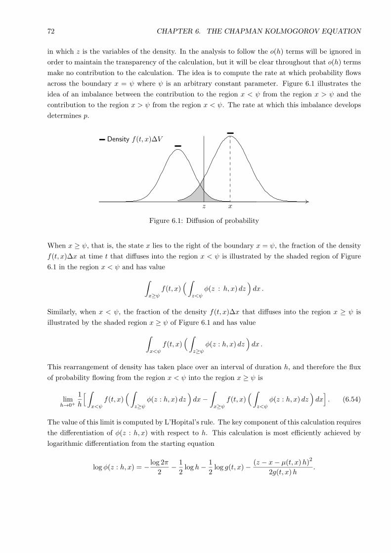
72 CHAPTER 6. THE CHAPMAN KOLMOGOROV EQUATION
in which z is the variables of the density. In the analysis to follow the o(h) terms will be ignored in
order to maintain the transparency of the calculation, but it will be clear throughout that o(h) terms
make no contribution to the calculation. The idea is to compute the rate at which probability flows
across the boundary x = ψ where ψ is an arbitrary constant parameter. Figure 6.1 illustrates the
idea of an imbalance between the contribution to the region x < ψ from the region x > ψ and the
contribution to the region x > ψ from the region x < ψ. The rate at which this imbalance develops
determines p.
z x
Density f(t, x)∆V
Figure 6.1: Diffusion of probability
When x ≥ ψ, that is, the state x lies to the right of the boundary x = ψ, the fraction of the density
f(t, x)∆x at time t that diffuses into the region x < ψ is illustrated by the shaded region of Figure
6.1 in the region x < ψ and has value∫x≥ψ
f(t, x)(∫
z<ψϕ(z : h, x) dz
)dx .
Similarly, when x < ψ, the fraction of the density f(t, x)∆x that diffuses into the region x ≥ ψ is
illustrated by the shaded region x ≥ ψ of Figure 6.1 and has value∫x<ψ
f(t, x)(∫
z≥ψϕ(z : h, x) dz
)dx .
This rearrangement of density has taken place over an interval of duration h, and therefore the flux
of probability flowing from the region x < ψ into the region x ≥ ψ is
limh→0+
1
h
[ ∫x<ψ
f(t, x)(∫
z≥ψϕ(z : h, x) dz
)dx−
∫x≥ψ
f(t, x)(∫
z<ψϕ(z : h, x) dz
)dx
]. (6.54)
The value of this limit is computed by L’Hopital’s rule. The key component of this calculation requires
the differentiation of ϕ(z : h, x) with respect to h. This calculation is most efficiently achieved by
logarithmic differentiation from the starting equation
log ϕ(z : h, x) = − log 2π
2− 1
2log h− 1
2log g(t, x)− (z − x− µ(t, x)h)2
2g(t, x)h.
6.4. ALTERNATIVE VIEW OF THE FORWARD KOLMOGOROV EQUATION 73
Differentiation with respect to h and with respect to zj gives
1
ϕ
∂ϕ
∂h= − 1
2h+µ(t, x)(zk − xk − µk h)
g(t, x)h+
(z − x− µ(t, x)h)2
2g(t, x)h2.
1
ϕ
∂ϕ
∂z= −(z − x− µ(t, x)h)
g(t, x)h.
(6.55)
Evidently the previous results can be combine to show that ϕ(z : h, x) satisfies the identity
∂ϕ
∂h= − 1
2hϕ− µ(t, x)
∂ϕ
∂z− 1
2h(z − x− µ(t, x)h)
∂ϕ
∂z
= − 1
2h
∂[(z − x+ µ(t, x)h)ϕ]
∂z.
(6.56)
In view of identity (6.59), L’Hopital’s rule applied to equation (6.54) gives
p = limh→0+
[ 1
2h
∫x<ψ
f(t, x)[−
∫z≥ψ
∂[(z − x+ µ(t, x)h)ϕ]
∂zdz
]dx
+1
2h
∫x≥ψ
f(t, x)[ ∫
z<ψ
∂[(z − x+ µ(t, x)h)ϕ]
∂zdz
]dx
],
= limh→0+
1
2h
[−
∫x<ψ
f(t, x)(− (ψ − x+ µ(t, x)h)ϕ
)dx
+
∫x≥ψ
f(t, x)((ψ − x+ µ(t, x)h)ϕ
)dx
].
(6.57)
Further simplification gives
p = limh→0+
1
2h
∫Rf(t, x) (ψ − x+ µ(t, x)h)ϕ(ψ;x, h) dx . (6.58)
One way to make further progress is to compute the integral of p with respect to ψ over the [a, b ] such
that a < ψ < b, that is, the point ψ is guaranteed to lie within the interval [a, b ]. The computation
of this integral will require the evaluation of
I =
∫ b
a
(ψ − x+ µ(t, x)h
2h√g(t, x)h
)exp
(− (ψ − x− µ(t, x)h)2
2g(t, x)h
)dψ .
Under the change of variable y = (ψ − x− µ(t, x))/√g(t, x)h, the integral for I becomes
I =
∫ (b−x−µ(t,x)h)/√g(t,x)h
(a−x−µ(t,x)h)/√g(t,x)h
(µ(t, x) +
y√g(t, x)h
2h
)e−y
2/2 dy ,
and therefore
I = µ(t, x)[Φ(b− x− µ(t, x)h√
g(t, x)h
)− Φ
(a− x− µ(t, x)h√g(t, x)h
)]+
√g(t, x)h
2h
∫ b−x−µ(t,x)h)/√g(t,x)h
a−x−µ(t,x)h)/√g(t,x)h
ye−y2/2 dy
= µ(t, x)[Φ(b− x− µ(t, x)h√
g(t, x)h
)+Φ
(a− x− µ(t, x)h√g(t, x)h
)]+
√g(t, x)h
2h
[exp
(− (b− x− µ(t, x)h)2
2g(t, x)h
)− exp
(− (a− x− µ(t, x)h)2
2g(t, x)h
) ].
74 CHAPTER 6. THE CHAPMAN KOLMOGOROV EQUATION
The conclusion of this calculation is that∫ b
ap(t, ψ) dψ = lim
h→0+
∫Rf(x)µ(t, x)
[Φ(b− x− µ(t, x)h√
g(t, x)h
)− Φ
(a− x− µ(t, x)h√g(t, x)h
)]dx
− limh→0+
∫Rf(x)
√g(t, x)h
2h
[exp
(− (b− x− µ(t, x)h)2
2g(t, x)h
)− exp
(− (a− x− µ(t, x)h)2
2g(t, x)h
) ]dx .
Now consider the value of the limit under each integral. First, it is clear that
limh→0+
[Φ(b− x− µ(t, x)h√
g(t, x)h
)− Φ
(a− x− µ(t, x)h√g(t, x)h
)]=
[0 x ∈ (−∞, a) ∪ (b,∞)
1 x ∈ [a, b ]
Second,
limh→0+
1√g(t, x)h
exp(− (b− x− µ(t, x)h)2
2g(t, x)h
)= δ(x− b) ,
limh→0+
1√g(t, x)h
exp(− (a− x− µ(t, x)h)2
2g(t, x)h
)= δ(x− a) .
These limiting values now give that∫ b
ap(t, ψ) dψ =
∫ b
af(t, x)µ(t, x) dx−
∫Rf(t, x)
[g(t, x)δ(x− b)− g(t, x)δ(x− a)
]dx
=
∫ b
af(t, x)µ(t, x) dx− [f(t, b)g(t, b)− f(t, a)g(t, a) ] .
(6.59)
Equation (6.59) is now divided by (b − a) and limits taken such that (b − a) → 0+ while retaining
the point ψ within the interval [a.b ]. The result of this calculation is that
p(t, ψ) = µ(t, ψ)f(t, ψ)− ∂ [ g(t, ψ)f(t, ψ) ]
∂ψ. (6.60)
Chapter 7
Numerical Integration of SDE
The dearth of closed form solutions to stochastic differential equations means that numerical proce-
dures enjoy a prominent role in the development of the subject.
7.1 Issues of convergence
The definition of convergence for a stochastic process is more subtle than the equivalent definition
in a deterministic environment, primarily because stochastic processes, by their very nature, cannot
be constrained to lie within ε of the limiting value for all n > N . Several types of convergence are
possible in a stochastic environment.
The first measure is based on the observation that although individual paths of a stochastic process
behave randomly, the expected value of the process, normally estimated numerically as the average
value over a large number of realisations of the process under identical conditions, behaves determin-
istically. This observation can be used to measure convergence in the usual way. The central limit
theorem indicates that if the variance of the process is finite, then convergence to the expected state
will follow a square-root N law where N is the number of repetitions.
7.1.1 Strong convergence
Suppose that X(t) is the actual solution of an SDE and Xn(t) is the solution based on an iterative
scheme with step size ∆t, we say that Xn exhibits strong convergence to X of order α if
E [ |Xn −X | ] < C (∆t)α (7.1)
Given a numerical procedure to integrate an SDE, we may identify the order of strong convergence
by the following numerical procedure.
1. Choose ∆t and integrate the SDE over an interval of fixed length, say T , many times.
75
76 CHAPTER 7. NUMERICAL INTEGRATION OF SDE
2. Compute the left hand side of inequality (7.1) and repeat this process for different values of ∆t.
3. Regress the logarithm of the left hand side of (7.1) against log(∆t).
If strong convergence of order α is present, the gradient of this regression line will be significant and
its value will be α, the order of strong convergence.
Although it might appear superficially that strong convergence is about expected values and not
about individual solutions, the Markov inequality
Prob ( |X| ≥ A) ≤ E [ |X| ]A
(7.2)
indicates that the presence of strong convergence of order α offers information about individual
solutions. Take A = (∆t)β then clearly
Prob ( |Xn −X | ≥ (∆t)β) ≤ E [ |Xn −X | ](∆t)β
≤ C (∆t)α−β (7.3)
or equivalently
Prob ( |Xn −X | < (∆t)β ) > 1− C (∆t)α−β . (7.4)
For example, take β = α−ε where ε > 0, then the implication of the Markov inequality in combination
with strong convergence is that the solution of the numerical scheme converges to that of the SDE
with probability one as ∆t→ 0 - hence the term strong convergence.
7.1.2 Weak convergence
Strong convergence imposes restrictions on the rate of decay of the mean-of-the-error to zero as
∆t → 0. By contrast, weak convergence involves the error-of-the-mean. Suppose that X(t) is the
actual solution of an SDE and Xn(t) is the solution based on an iterative scheme with step size ∆t,
Xn is said to converge weakly to X with order α if
|E [ f(Xn) ]− E [ f(X) ] | < C (∆t)α (7.5)
where the condition is required to be satisfied for all function f belonging to a prescribed class C of
functions. The identify function f(x) = x is one obvious choice of f . Another choice for C is the class
of functions satisfying prescribed properties of smoothness and polynomial growth.
Clearly the numerical experiment that was described in the section concerning strong convergence
can be repeated, except that the objective of the calculation is now to find the difference in expected
values for each ∆t and not the expected value of differences.
Theorem Let X(t) be an n-dimensional random variable which evolves in accordance with the
stochastic differential equation
dx = a(t,x) dt+B(t,x) dW , x(t0) = X0 (7.6)
7.2. DETERMINISTIC TAYLOR EXPANSIONS 77
where B(t,x) is an n × m array and dW is an m-dimensional vector of Wiener increments, not
necessarily uncorrelated. If a(t,x) and B(t,x) satisfy the conditions
||ϕ(t,x)− ϕ(t,y)|| ≤ c||x− y|| , ||ϕ(t,x)|| ≤ c(1 + ||x||)
for constant c, then the initial value problem (7.6) has a solution in the vicinity of t = t0, and this
solution is unique.
7.2 Deterministic Taylor Expansions
The Taylor series expansion of a function of a deterministic variable is well known. Since the existence
of the Taylor series is a property of the function and not the variable in which the function is
expanded, then the Taylor series of a function of a stochastic variable is possible. As a preamble to
the computation of these stochastic expansions, the procedure is first described in the context of an
expansion in a deterministic function.
Suppose xi(t) satisfies the differential equation dxi/dt = ai(t,x) and let f : R → R be a continuously
differentiable function of t and x then the chain rule gives
df
dt=∂f
∂t+
n∑k=1
∂f
∂xk
dxkdt
=∂f
∂t+
n∑k=1
ak∂f
∂xk−→ df
dt= Lf (7.7)
where the linear operator L is defined in the obvious way. By construction,
f(t,xt) = f(t0,x0) +
∫ t
t0
Lf(s,xs) ds ,
xt = x0 +
∫ t
t0
a(s,xs) ds .
(7.8)
Now apply result (7.8) to a(t,xt) to obtain
a(s,xs) = a(t0,x0) +
∫ s
t0
La(u,xu) du , (7.9)
and this result, when incorporated into (7.8) gives
xt = x0 +
∫ t
t0
(a(t0,x0) +
∫ s
t0
La(u,xu) du
)ds
= x0 + a(t0,x0)
∫ t
t0
ds+
∫ t
t0
∫ s
t0
La(u,xu) du ds .
(7.10)
The process is now repeated with f in equation (7.8) replaced with La(u, xu). The outcome of this
operation is
xt = x0 + a(t0,x0)
∫ t
t0
ds+
∫ t
t0
∫ s
t0
La(u,xu) du ds
= x0 + a(t0,x0)
∫ t
t0
ds+
∫ t
t0
∫ s
t0
(La(t0,x0) +
∫ u
t0
L2a(w,xw) dw
)du ds
= x0 + a(t0,x0)
∫ t
t0
ds+ La(t0,x0)
∫ t
t0
∫ s
t0
du ds+
∫ u
t0
∫ t
t0
∫ s
t0
L2a(w,xw) dw du ds
(7.11)
78 CHAPTER 7. NUMERICAL INTEGRATION OF SDE
The procedure may be repeated provided the requisite derivatives exist. By recognising that∫ t
t0
∫ u
t0
· · ·∫ s
t0
dw · · · du =(t− t0)
k
k!
it follows directly from (7.11) that
xt = x0 + a(t0,x0) t+ La(t0,x0)(t− t0)
2
2+R3 , R3 =
∫ u
t0
∫ t
t0
∫ s
t0
L2a(w,xw) dw du ds . (7.12)
7.3 Stochastic Ito-Taylor Expansion
The idea developed in the previous section for deterministic Taylor expansions will now be applied to
the calculation of stochastic Taylor expansions. Suppose that x(t) satisfies the initial value problem
dxk = ak(t,x) dt+ bk α(t,x) dWαt , x(0) = x0 . (7.13)
The first task is to differentiate f(t,x) with respect to t using Ito’s Lemma. The general Ito result is
derived from the Taylor expansion
df =∂f
∂tdt+
n∑k=1
∂f
∂xkdxk +
1
2
[ ∂2f∂t2
(dt)2 + 2
n∑k=1
∂2f
∂t∂xkdt dxk +
n∑j,k=1
∂2f
∂xj∂xkdxk dxj
]+ · · · .
The idea is to expand this expression to order dt, ignoring all terms of order higher than dt since
these will vanish in the limiting process. The first step in the derivation of Ito’s lemma is to replace
dxk from the stochastic differential equation (7.13) in the previous equation. All terms which are
overtly o(dt) are now discarded to obtain the reduced equation
df =∂f
∂tdt+
n∑k=1
∂f
∂xk
[ak(t,x) dt+ bk α(t,x) dW
αt
]+
1
2
[ n∑j,k=1
∂2f
∂xj∂xkbk α(t,x) dW
αt bj β(t,x) dW
βt
]+ · · ·
For simplicity, now suppose that dWα are uncorrelated Wiener increments so that
df =[ ∂f∂t
+
n∑k=1
∂f
∂xkak(t,x) +
1
2
n∑j,k=1
∂2f
∂xj∂xkb k α(t,x) bj α(t,x)
]dt+
n∑k=1
∂f
∂xkb k α(t,x) dW
αt
which in turn leads to the integral form
f(t, xt) = f(t0, x0) +
∫ t
t0
L0 f(s,xs) ds+
∫ t
t0
Lα f(s,xs) dWαs (7.14)
in which the linear operators L0 and Lα are defined by the formulae
L0 f =∂f
∂t+
n∑k=1
∂f
∂xkak(t,x) +
1
2
n∑j,k=1
∂2f
∂xj∂xkb k α(t,x) bj α(t,x) ,
Lα f =
n∑k=1
∂f
∂xkb k α(t,x) .
(7.15)
7.3. STOCHASTIC ITO-TAYLOR EXPANSION 79
In terms of these operators, it now follows that
f(t,xt) = f(t0,x0) +
∫ t
t0
L0 f(s,xs) ds+
∫ t
t0
Lα f(s,xs) dWαs (7.16)
xk(t) = xk(0) +
∫ t
t0
ak(s,xs) ds+
∫ t
t0
b k α(s,xs) dWαs . (7.17)
By analogy with the treatment of the deterministic case, the Ito formula (7.16) is now applied to
ak(t,x) and b k α(t,x) to obtain
ak(t,xt) = ak(t0,x0) +
∫ t
t0
L0 ak(s,xs) ds+
∫ t
t0
Lα ak(s,xs) dWαs
b k α(t,xt) = b k α(t0,x0) +
∫ t
t0
L0 b k α(s,xs) ds+
∫ t
t0
Lβ b k α(s,xs) dWβs
(7.18)
Formulae (7.18) are now applied to the right hand side of equation (7.17) to obtain initially
xk(t) = xk(0) +
∫ t
t0
(ak(t0,x0) +
∫ s
t0
L0 ak(u,xu) du+
∫ s
t0
Lα ak(u,xu) dWαu
)ds
+
∫ t
t0
(b k α(t0,x0) +
∫ s
t0
L0 b k α(u,xu) du+
∫ s
t0
Lβ b k α(u,xu) dWβu
)dWα
s
which simplifies to the stochastic Taylor expansion
xk(t) = xk(0) + ak(t0,x0)
∫ t
t0
ds+ b k α(t0,x0)
∫ t
t0
dWαs +R
(2)k (7.19)
where R(2)k denotes the remainder term
R(2)k =
∫ t
t0
∫ s
t0
L0 ak(u,xu) du ds+
∫ t
t0
∫ s
t0
Lα ak(u,xu) dWαu ds
+
∫ t
t0
∫ s
t0
L0 b k α(u,xu) du dWαs +
∫ t
t0
∫ s
t0
Lβ b k α(u,xu) dWβu dW
αs .
(7.20)
Each term in the remainder R2 may now be expanded by applying the Ito expansion procedure (7.16)
in the appropriate way. Clearly,∫ t
t0
∫ s
t0
L0 ak(u,xu) du ds = L0 ak(t0,x0)
∫ t
t0
∫ s
t0
du ds
+
∫ t
t0
∫ s
t0
∫ u
t0
L0L0 ak(w,xw) dw du ds+
∫ t
t0
∫ s
t0
∫ u
t0
Lγ L0 ak(w,xw) dWγw du ds
∫ t
t0
∫ s
t0
Lα ak(u,xu) dWαu ds = Lα ak(t0,x0)
∫ t
t0
∫ s
t0
dWαu ds
+
∫ t
t0
∫ s
t0
∫ u
t0
L0 Lα ak(w,xw) dw dWαu ds+
∫ t
t0
∫ s
t0
∫ u
t0
Lγ Lα ak(w,xw) dWγw dW
αu ds
∫ t
t0
∫ s
t0
L0 b k α(u,xu) du dWαs = L0 b k α(t0,x0)
∫ t
t0
∫ s
t0
du dWαs
80 CHAPTER 7. NUMERICAL INTEGRATION OF SDE
+
∫ t
t0
∫ s
t0
∫ u
t0
L0L0 b k α(w,xw) dw du dWαs +
∫ t
t0
∫ s
t0
∫ u
t0
Lγ L0b k α(w, xw) dWγw du dW
αs
∫ t
t0
∫ s
t0
Lβ b k α(u,xu) dWβu dW
αs = Lβ b k α(t0,x0)
∫ t
t0
∫ s
t0
dW βu dW
αs
+
∫ t
t0
∫ s
t0
∫ u
t0
L0 Lβ b k α(w, xw) dw dWβu dW
αs +
∫ t
t0
∫ s
t0
∫ u
t0
Lγ Lβ b k α(w, xw) dWγw dW
βu dW
αs .
The general principle is apparent in this expansion. One must evaluate stochastic integrals involving
combinations of deterministic (du) and stochastic (dW ) differentials. For our purposes, it is enough
to observe that
xk(t) = xk(0) + ak(t0,x0)
∫ t
t0
ds+ b k α(t0,x0)
∫ t
t0
dWαs + L0 ak(t0,x0)
∫ t
t0
∫ s
t0
du ds
+ Lα ak(t0,x0)
∫ t
t0
∫ s
t0
dWαu ds+ L0 b k α(t0,x0)
∫ t
t0
∫ s
t0
du dWαs
+ Lβ b k α(t0,x0)
∫ t
t0
∫ s
t0
dW βu dW
αs +R
(3)k .
(7.21)
This solution can be expressed more compactly in terms of the multiple Ito integrals
Iijk··· =
∫ ∫· · ·
∫dW i dW j · · · dW k
where dW k = ds if k = 0 and dW k = dWαs if k = α > 0. Using this representation, the solution
(7.21) takes the short hand form
xk(t) = xk(0) + ak(t0,x0) I0 + b k α(t0,x0) Iα + L0 ak(t0,x0) I00 + Lα ak(t0,x0) Iα 0
+ L0 b k α(t0,x0) I0α + Lβ b k α(t0,x0) Iβ α +R(3)k .
(7.22)
7.4 Stochastic Stratonovich-Taylor Expansion
The analysis developed in the previous section for the Ito stochastic differential equation
dxk = ak(t,x) dt+∑α
bk α(t,x) dWαt , x(0) = x0 . (7.23)
can be repeated for the Stratonovich representation of equation (7.23), namely,
dxk = ak(t,x) dt+∑α
bk α(t,x) dWαt , x(0) = x0 . (7.24)
in which
ai = ai −1
2
∑k,α
b k α∂b i α∂xk
.
The first task is to differentiate f(t,x) with respect to t using the Stratonovich form of Ito’s Lemma.
It can be demonstrated for uncorrelated Wiener increments dWα that
f(t, xt) = f(t0, x0) +
∫ t
t0
L0 f(s,xs) ds+
∫ t
t0
Lα f(s,xs) dWαs (7.25)
7.5. EULER-MARUYAMA ALGORITHM 81
in which the linear operators L0 and Lα are defined by the formulae
L0 f =∂f
∂t+
∑k
∂f
∂xkak(t,x) , Lα f =
∑k
∂f
∂xkb k α(t,x) . (7.26)
In terms of these operators, it now follows that
f(t,xt) = f(t0,x0) +
∫ t
t0
L0 f(s,xs) ds+
∫ t
t0
Lα f(s,xs) dWαs (7.27)
xk(t) = xk(0) +
∫ t
t0
ak(s,xs) ds+
∫ t
t0
b k α(s,xs) dWαs . (7.28)
The analysis of the previous section is now repeated to yield
xk(t) = xk(0) + ak(t0,x0)
∫ t
t0
ds+ b k α(t0,x0)
∫ t
t0
dWαs + L0 ak(t0,x0)
∫ t
t0
∫ s
t0
du ds
+ Lα ak(t0,x0)
∫ t
t0
∫ s
t0
dWαu ds+ L0 b k α(t0,x0)
∫ t
t0
∫ s
t0
du dWαs
+ Lβ b k α(t0,x0)
∫ t
t0
∫ s
t0
dW βu dWα
s +R(3)k .
(7.29)
This solution can be expressed more compactly in terms of the multiple Stratonovich integrals
Jijk··· =
∫ ∫· · ·
∫ dW i dW j · · · dW k
where dW k = ds if k = 0 and dW k = dWαs if k = α > 0. Using this representation, the solution
(7.29) takes the short hand form
xk(t) = xk(0) + ak(t0,x0) J0 +∑α
b k α(t0,x0) Jα + L0 ak(t0,x0) J00
+∑α
Lα ak(t0,x0) Jα 0L0 b k α(t0,x0) J0α +
∑α,β
Lβ b k α(t0,x0) Jβ α +R(3)k .
(7.30)
7.5 Euler-Maruyama algorithm
The Euler-Maruyama algorithm is the simplest numerical scheme for the solution of SDE’s, being
the stochastic equivalent of the deterministic Euler scheme. The algorithm is
xk(t) = xk(0) + ak(t0,x0) I0 +∑α
b k α(t0,x0) Iα . (7.31)
It follows directly from the definitions of Iijk··· that
I0 = (t− t0) , Iα =Wα(t)−Wα(t0)
and consequently
xk(t) = xk(0) + ak(t0,x0) (t− t0) +∑α
b k α(t0,x0) (Wα(t)−Wα(t0)) . (7.32)
82 CHAPTER 7. NUMERICAL INTEGRATION OF SDE
In practice, the interval [a, b] is divided into n subintervals of length h where h = (b − a)/n. The
Euler-Maruyama scheme now becomes
xj+1k = xjk + ak(tj ,xj)h+
∑α
b k α(tj ,xj)∆Wαj , ∆Wα
j ∼ N(0,√h) (7.33)
where xjk denotes the value of the k-th component of x at time tj = t0 + jh. It may be shown that
the Euler-Maruyama has strong order of convergence γ = 1/2 and weak order of convergence γ = 1.
7.6 Milstein scheme
The principal determinant of the accuracy of the Euler-Maruyama is the stochastic term which is in
practice√h accurate. Therefore, to improve the quality of the Euler-Maruyama scheme, one should
first seek to improve the accuracy of the stochastic term. Equation (7.22) indicates that the accuracy
of the Euler-Maruyama scheme can be improved by including the term∑α,β
Lβ b k α(t0,x0) Iβ α
in the Euler-Maruyama algorithm (7.33). This now requires the computation of
Iβ α =
∫ t
t0
∫ s
t0
dW βu dW
αs =
∫ t
t0
(W β(s)−W β(t0)) dWαs .
When α = β, it has been seen in previous analysis that
Iαα =
∫ t
t0
(Wα(s)−Wα(t0)) dWαs
=1
2
[(Wα(t))2 − (Wα(t0))
2 − (t− t0)]−Wα(t0) (W
α(t)−Wα(t0))
=1
2
[ (Wα(t)−Wα(t0)
)2− (t− t0)
].
When α = β, however, Iαβ is not just a combination of (Wα(s)−Wα(t0)) and (W β(s)−W β(t0)). The
value must be approximated even in this apparently straightforward case. Therefore, the numerical
solution of systems of SDEs in which the evolution of the solution is characterised by more than one
independent stochastic process is likely to be numerically intensive by any procedure other than the
Euler-Maruyama algorithm. However, one exception to this working rule occurs whenever symmetry
is present in the respect that
Lβ b k α(t0,x0) = Lα b k β(t0,x0) .
In this case,
Lβ b k α(t0,x0) Iβ α =1
2Lβ b k α(t0,x0) ( Iβ α + Iαβ )
which can now be computed from the identity
Iβ α + Iαβ = (W β(t)−W β(t0) )(Wα(t)−Wα(t0) ) .
7.6. MILSTEIN SCHEME 83
For systems of SDEs governed by a single Wiener process, it is relatively easy to develop higher order
schemes. For the system
dxk = ak(t,x) dt+ bk(t,x) dWt , x(0) = x0 (7.34)
the Euler-Maruyama algorithm is
xj+1k = xjk + ak(tj ,xj)h+ bk(tj ,xj)∆Wj , ∆Wj ∼ N(0,
√h) (7.35)
and the Milstein improvement to this algorithm is
xj+1k = xjk+ak(tj ,xj)h+ bk(tj ,xj)∆Wj +
1
2L1 bk(tj ,xj) [ (∆Wj)
2−h] , ∆Wj ∼ N(0,√h) . (7.36)
The operator L1 is defined by the rule L1 f =∑
k∂f∂xk
bk(t,x) and this in turn yields the Milstein
scheme
xj+1k = xjk + ak(tj ,xj)h+ bk(tj ,xj)∆Wj +
1
2
∑n
bn∂bk(tj ,xj)
∂xn[ (∆Wj)
2 − h] , (7.37)
where ∆Wj ∼ N(0,√h). For example, in one dimension, the SDE dx = a dt+ b dWt gives rise to the
Milstein scheme
xj+1 = xj + a(tj , xj)h+ b(tj , x
j)∆Wj +b
2
db(tj , xj)
dx[ (∆Wj)
2 − h] , ∆Wj ∼ N(0,√h) . (7.38)
7.6.1 Higher order schemes
For general systems of SDEs its already clear that higher order schemes are difficult unless the
equations possess a high degree of symmetry. Whenever the SDEs are dependent on a single stochastic
process, some progress may be possible. To improve upon the Milstein scheme, it is necessary to
incorporate all terms which behave like h3/2 into the numerical scheme. Expression (7.22) overtly
contains two such terms in
Lα ak(t0,x0) Iα 0 + L0 b k α(t0,x0) I0α
but there is one further term hidden in R(3)k , namely
Lγ Lβ b k α(t0, x0)
∫ t
t0
∫ s
t0
∫ u
t0
dW γw dW
βu dW
αs = Lγ Lβ b k α(t0, x0) Iγ β α .
Restricting ourselves immediately to the situation of a single Wiener process, the additional terms
to be added to Milstein’s scheme to improve the accuracy to a strong Taylor scheme of order 3/2 are
L1 ak(t0,x0) I10 + L0 bk(t0,x0) I01 + L1 L1 bk(t0, x0) I111 (7.39)
in which the operators L0 and L1 are defined by
L0 f =∂f
∂t+
∑k
∂f
∂xkak(t,x) +
1
2
∑j,k
∂2f
∂xj∂xkbk(t,x) bj(t,x) , L1 f =
∑k
∂f
∂xkbk(t,x) . (7.40)
84 CHAPTER 7. NUMERICAL INTEGRATION OF SDE
The values of I01, I10 and I111 have been computed previously in the exercises of Chapter 4 for the
interval [a, b]. The relevant results with respect to the interval [t0, t] are
I10 + I01 = (t− t0)(Wt −W0) ,
I111 =(Wt −W0)
6
[(Wt −W0)
2 − 3(t− t0)].
(7.41)
Formulae (7.41) determine the coefficients of the new terms to be added to Milstein’s algorithm to
generate a strong Taylor approximation of order 3/2. Of course, the Riemann integral I10 must still
be determined. This calculation is included as a problem in Chapter 4, but its outcome is that I10
is a Gaussian process with a mean value of zero, variance (t− t0)3/3 and has correlation (t− t0)
2/2
with (Wt −W0). Thus ∆Zj = I10 may be simulated as a Gaussian deviate with mean zero, variance
h3/3 and such that it has correlation h2/2 with ∆Wj . The extra terms are
∑m
bm ak ,m∆Zj +[ ∂bk∂t
+∑m
am∂bk∂xm
+1
2
∑m,r
bm br∂2bk
∂xm∂xr
](h∆Wj −∆Zj)
+1
6
∑r,m
br∂
∂xr
(bm
∂bk∂xm
)(∆Wj)[ (∆Wj)
2 − 3h ](7.42)
where all derivatives are understood to be evaluated at time tj and state xj . Consider, for example,
the simplest scenario of a single equation. In this case, the extra terms (7.42) become
b a′∆Zj +[bt + a b′ +
1
2b2 b′′ ] (h∆Wj −∆Zj) +
1
6b ( b b′)′ (∆Wj)[ (∆Wj)
2 − 3h ]
= b a′∆Zj +[bt + a b′ +
1
2b2 b′′ ] (h∆Wj −∆Zj) +
b
2[ (b′)2 + b′′ ] [
(∆Wj)2
3− h ]∆Wj .
(7.43)
Chapter 8
Exercises on SDE
Exercises on Chapter 2
Q 1. LetW1(t) andW2(t) be two Wiener processes with correlated increments ∆W1 and ∆W2 such
that E [∆W1∆W2] = ρ∆t. Prove that E [W1(t)W2(t)] = ρ t. What is the value of E [W1(t)W2(s)]?
Q 2. Let W (t) be a Wiener process and let λ be a positive constant. Show that λ−1W (λ2t) and
tW (1/t) are each Wiener processes.
Q 3. Suppose that (ε1 , ε2) is a pair of uncorrelated N (0, 1) deviates.
(a) By recognising that ξx = σx ε1 has mean value zero and variance σ2x, construct a second deviate
ξy with mean value zero such that the Gaussian deviate X = [ ξx , ξy ]T has mean value zero
and correlation tensor
Ω =
σ2x ρ σxσy
ρ σxσy σ2y
where σx > 0, σy > 0 and | ρ | < 1.
(b) Another possible way to approach this problem is to recognise that every correlation tensor is
similar to a diagonal matrix with positive entries. Let
α =σ2x − σ2y
2, β =
1
2
√(σ2x + σ2y)
2 − 4(1− ρ2)σ2xσ2y =
√α2 − ρ2σ2xσ
2y .
Show that
Q =1√2β
√β + α −
√β − α√
β − α√β + α
is an orthogonal matrix which diagonalises Ω, and hence show how this idea may be used to
find X = [ ξx , ξy ]T with the correlation tensor Ω.
85
86 CHAPTER 8. EXERCISES ON SDE
(c) Suppose that (ε1, . . . , εn) is a vector of n uncorrelated Gaussian deviates drawn from the dis-
tribution N (0, 1). Use the previous idea to construct an n-dimensional random column vector
X with correlation structure Ω where Ω is a positive definite n× n array.
Q 4. Let X be normally distributed with mean zero and unit standard deviation, then Y = X2 is
said to be χ2 distributed with one degree of freedom.
(a) Show that Y is Gamma distribution with λ = ρ = 1/2.
(b) What is now the distribution of Z = aX2 if a > 0 and X ∼ N(0, σ2).
(b) If X1, · · · , Xn are n independent Gaussian distributed random variables with mean zero and
unit standard deviation, what is the distribution of Y = XTX where X is the n dimensional
column vector whose k-th entry is Xk.
Exercises on Chapter 3
Q 5. Calculate the bounded variation (when it exists) for the functions
(a) f(x) = |x| x ∈ [−1, 2] (b) g(x) = log x x ∈ (0, 1]
(c) h(x) = 2x3 + 3x2 − 12x+ 5 x ∈ [−3, 2] (d) k(x) = 2 sin 2x x ∈ [π/12, 5π/4]
(e) n(x) = H(x)−H(x− 1) x ∈ R (f) m(x) = (sin 3x)/x x ∈ [−π/3, π/3] .
Q 6. Use the definition of the Riemann integral to demonstrate that
(a)
∫ 1
0x dx =
1
2, (b)
∫ 1
0x2 dx =
1
3.
You will find useful the formulae∑n
k=1 k = n(n+ 1)/2 and∑n
k=1 k2 = n(n+ 1)(2n+ 1)/6.
Q 7. The functions f , g and h are defined on [0, 1] by the formulae
(a) f(x) =
x sin(π/x) x > 0
0 x = 0
(b) g(x) =
x2 sin(π/x) x > 0
0 x = 0
(c) h(x) =
(x/ log x) sin(π/x) x > 0
0 x = 0, 1
Determine which functions have bounded variation on the interval [0, 1].
87
Exercises on Chapter 4
Q 8. Prove that ∫ b
a(dWt)
2G(t) =
∫ b
aG(t) dt
Q 9. Prove that ∫ b
aWn dWt =
1
n+ 1
[W (b)n+1 −W (a)n+1
]− n
2
∫ b
aWn−1 dt .
Q 10. The connection between the Stratonovich and Ito integrals relied on the claim that
limn→∞
E[ n∑k=1
∂f(tk−1Wk−1)
∂W
((Wk−1/2 −Wk−1)(Wk −Wk−1)−
tk − tk−1
2
) ]2= 0
provided E [ |∂f(t,W )/∂W |2 ] is integrable over the interval [a, b]. Verify this unsubstantiated claim.
Q 11. Compute the value of
Φ =
∫ b
aWt dWt
where the definition of the integral is based on the choice ξk = (1− λ)tk−1 + λtk and λ ∈ [0, 1].
Q 12. Solve the stochastic differential equation
dxt = a(t) dt+ b(t) dWt , x0 = X0
where X0 is constant. Show that the solution xt is a Gaussian deviate and find its mean and variance.
Q 13. The stochastic integrals I01 and I10 defined by
I10 =
∫ b
a
∫ s
0dWu ds , I01 =
∫ b
a
∫ s
0du dWs .
occur frequently in the numerical solution of stochastic differential equations. Show that
I10 + I01 = (b− a)(Wb −Wa) .
Q 14. The stochastic integrals I111 defined by
I111 =
∫ t
a
∫ s
a
∫ u
adWw dWu dWs
occurs frequently in the numerical solution of stochastic differential equations. Show that
I111 =(Wb −Wa)
6
[(Wb −Wa)
2 − 3(b− a)].
Q 15. Show that the value of the Riemann integral
I10 =
∫ b
a
∫ s
0dWu ds
may be simulated as a Gaussian deviate with mean value zero, variance (b− a)3/3 and such that its
correlation with (Wb −Wa) is (b− a)2/2.
88 CHAPTER 8. EXERCISES ON SDE
Exercises on Chapter 5
Q 16. Solve the degenerate Ornstein-Uhlenbeck stochastic initial value problem
dx = −αx+ σ dW , x(0) = x0
in which α and σ are positive constants and x0 is a random variable. Deduce that
E [X ] = E [x0 ] e−α t , V [X ] = V [x0 ] e
−2αt +σ2
2α[ 1− e−2αt) ] .
Q 17. It is given that the instantaneous rate of interest satisfies the equation
dr = µ(t, r) dt+√g(t, r) dW . (8.1)
Let B(t, R) be the value of a zero-coupon bond at time t paying one dollar at maturity T . Show that
B(t, R) is the solution of the partial differential equation
∂B
∂t+ µ(t, r)
∂B
∂r+g(t, r)
2
∂2B
∂r2= rB (8.2)
with terminal boundary condition B(T, r) = 1.
Q 18. It is given that the solution of the initial value problem
dx = −αx+ σ x dW , x(0) = x0
in which α and σ are positive constants is
x(t) = x(0) exp[− (α+ σ2/2)t+ σW (t)
]Show that
E [X ] = x0 e−α t , V [X ] = e−2α t(eσ
2 t − 1)x20 .
Q 19. Benjamin Gompertz (1840) proposed a well-known law of mortality that had the important
property that financial products based on male and female mortality could be priced from a single
mortality table with an age decrement in the case of females. Cell populations are also well-know to
obey Gompertzian kinetics in which N(t), the population of cells at time t, evolves according to the
ordinary differential equationdN
dt= αN log
(MN
),
where M and α are constants in which M represents the maximum resource-limited population of
cells. Write down the stochastic form of this equation and deduce that ψ = logN satisfies an OU
process. Further deduce that mean reversion takes place about a cell population that is smaller than
M , and find this population.
89
Q 20. A two-factor model of the instantaneous rate of interest, r(t), proposes that r(t) = r1(t)+r2(t)
where r1(t) and r2(t) satisfy the square-root processes
dr1 = α1(θ1 − r1) dt+ σ1√r1 dW1 ,
dr2 = α2(θ2 − r2) dt+ σ2√r2 dW2 ,
(8.3)
in which dW1 and dW2 are independent increments in the Wiener processes W1 and W2. Let
B(t, R1, R2) be the value of a zero-coupon bond at time t paying one dollar at maturity T .
Construct the partial differential equation satisfied by B(t, R1, R2) and write down the terminal
boundary condition for this equation.
Q 21. Solve the stochastic differential equation
dxt = a(t) dt+ b(t) dWt , x0 = X0
where X0 is constant. Show that the solution xt is a Gaussian deviate and find its mean and variance.
Q 22. Solve the stochastic differential equation
dxt = − xt dt
1 + t+dWt
1 + t, x0 = 0 .
Q 23. Solve the stochastic differential equation
dxt = −xt dt2
+√1− x2t dWt , x0 = a ∈ [−1, 1] .
Q 24. Solve the stochastic differential equation
dxt = dt+ 2√xt dWt , x(0) = x0 .
Q 25. Solve the stochastic differential equation
dx = [ a(t) + b(t)x ] dt+ [ c(t) + d(t)x ] dWt
by making the change of variable y(t) = x(t)ϕ(t) where ϕ(t) is to be chosen appropriately.
Q 26. In an Ornstein-Uhlenbeck process, x(t), the state of a system at time t, satisfies the stochastic
differential equation
dx = −α(x−X) dt+ σ dWt
where α and σ are positive constants and X is the equilibrium state of the system in the absence of
system noise. Solve this SDE. Use the solution to explain why x(t) is a Gaussian process, and deduce
its mean and variance.
90 CHAPTER 8. EXERCISES ON SDE
Q 27. Let x = (x1, . . . , xn) be the solution of the system of Ito stochastic differential equations
dxk = ak dt+ bk α dWα
where the repeated Greek index indicates summation from α = 1 to α = m. Show that x =
(x1, . . . , xn) is the solution of the Stratonovich system
dxk =[ak −
1
2bj αbk α,j
]dt+ bk α dWα .
Let ϕ = ϕ(t,x) be a suitably differentiable function of t and x. Show that ϕ is the solution of the
stochastic differential equation
dϕ =[ ∂ϕ∂t
+ ak∂ϕ
∂xk
]dt+
∂ϕ
∂xkbk α dWα
where ak = ak − bk α,j bj α/2.
Q 28. The displacement x(t) of the harmonic oscillator of angular frequency ω satisfies x = −ω2x.
Let z = x+ iωx. Show that the equation for the oscillator may be rewritten
dz
dt= iωz .
The frequency of the oscillator is randomized by the addition of white noise of standard deviation
σ to give random frequency ω + σξ(t) where ξ ∼ N(0, 1). Determine now the stochastic differential
equation satisfied by z.
Solve this SDE under the assumption that it should be interpreted as a Stratonovich equation, and
use the solution to construct expressions for
(a) E [ z(t) ] (b) E [ z(t) z(s) ] (c) E [ z(t) z(s) ] .
Exercises on Chapter 6
Q 29. It has been established in a previous example that the price B(t, R) of a zero-coupon bond
at time t and spot rate R paying one dollar at maturity T satisfies the Bond Equation
∂B
∂t+ µ(t, r)
∂B
∂r+g(t, r)
2
∂2B
∂r2= rB
with terminal condition B(T, r) = 1 when the instantaneous rate of interest evolves in accordance
with the stochastic differential equation dr = µ(t, r) dt+√g(t, r) dW .
The popular square-root process proposed by Cox, Ingersol and Ross, commonly called the CIR
process, corresponds to the choices µ(t, r) = α(θ − r) and g(t, r) = σ2r. It is given that the anzatz
B(t, r) = exp[β0(T − r) + β1(T − t)r] is a solution of the Bond Equation in this case provided the
coefficient functions β0(T−t) and β1(T−t) satisfy a pair of ordinary differential equations. Determine
these equations with their boundary conditions.
91
Solve these ordinary differential equations and deduce the value of B(t, R) where R is the spot rate
of interest.
Q 30. In a previous exercise it has been shown that the price B(t, R1, R2) of a zero-coupon bond
at time t paying one dollar at maturity T satisfies the partial differential equation
∂B
∂t+ α1(θ1 − r1)
∂B
∂r1+ α2(θ2 − r2)
∂B
∂r2+σ21r12
∂2B
∂r21+σ22r22
∂2B
∂r22= (r1 + r2)B ,
when the instantaneous rate of interest, r(t), is driven by a two-factor model in which r(t) = r1(t) +
r2(t) in which r1(t) and r2(t) evolve stochastically in accordance with the equations
dr1 = α1(θ1 − r1) dt+ σ1√r1 dW1 ,
dr2 = α2(θ2 − r2) dt+ σ2√r2 dW2 ,
(8.4)
where dW1 and dW2 are independent increments in the Wiener processes W1 and W2.
Given that the required solution has generic solution B(t, r1, r2) = exp[β0(T − r) + β1(T − t)r1 +
β2(T − t)r2], construct the ordinary differential equations satisfied by the coefficient functions β0, β1
and β2. What are the appropriate initial conditions for these equations?
Q 31. The position x(t) of a particle executing a uniform random walk is the solution of the
stochastic differential equation
dxt = µdt+ σ dWt , x(0) = X ,
where µ and σ are constants. Find the density of x at time t > 0.
Q 32. The position x(t) of a particle executing a uniform random walk is the solution of the
stochastic differential equation
dxt = µ(t) dt+ σ(t) dWt , x(0) = X ,
where µ and σ are now prescribed functions of time. Find the density of x at time t > 0.
Q 33. The state x(t) of a particle satisfies the stochastic differential equation
dxt = a dt+ b dWt , x(0) = X ,
where a is a constant vector of dimension n, b is a constant n ×m matrix and dW is a vector of
Wiener increments with m×m covariance matrix Q. Find the density of x at time t > 0.
Q 34. The state x(t) of a system evolves in accordance with the stochastic differential equation
dxt = µx dt+ σ x dWt , x(0) = X ,
where µ and σ are constants. Find the density of x at time t > 0.
92 CHAPTER 8. EXERCISES ON SDE
Q 35. The state x(t) of a system evolves in accordance with the Ornstein-Uhlenbeck process
dx = −α (x− β) dt+ σ dWt , x(0) = X ,
where α, β and σ are constants. Find the density of x at time t > 0.
Q 36. If the state of a system satisfies the stochastic differential equation
dx = a(x, t) dt+ b(x, t) dW , x(0) = X ,
write down the initial value problem satisfied by f(x, t), the probability density function of x at time
t > 0. Determine the initial value problem satisfied by the cumulative density function of x.
Q 37. Cox, Ingersoll and Ross proposed that the instantaneous interest rate r(t) should follow the
stochastic differential equation
dr = α(θ − r)dt+ σ√r dW , r(0) = r0 ,
where dW is the increment of a Wiener process and α, θ and σ are constant parameters. Show that
this equation has associated transitional probability density function
f(t, r) = c(vu
)q/2e−(
√u−
√v)2 e−2
√uv Iq(2
√uv) ,
where Iq(x) is the modified Bessel function of the first kind of order q and the functions c, u, v and
the parameter q are defined by
c =2α
σ2(1− e−α(t−t0)), u = cr0 e
−α(t−t0) , v = cr , q =2αθ
σ2− 1 .
Exercises on Chapter 7
Q 38. Consider the problem of numerically integrating the stochastic differential equation
dx = a(t, x) dt+ b(t, x) dW , x(0) = X0 .
Develop an iterative scheme to integrate this equation over the interval [0, T ] using the Euler-
Maruyama algorithm.
It is well-know that the Euler-Maruyama algorithm has strong order of convergence one half and
weak order of convergence one. Explain what programming strategy one would use to demonstrate
these claims.
Q 39. Compute the stationary densities for the stochastic differential equations
(a) dX = (β − αX) dt+ σ√X dW
93
(b) dX = −α tanX dt+ σ dW
(c) dX = [(θ1 − θ2) cosh(X/2)− (θ1 + θ2) sinh(X/2)] cosh(X/2) dt+ 2 cosh(X/2) dW
(d) dX =α
Xdt+ dW
(e) dX =( αX
−X)dt+ dW