Numerical modeling and Computational simulation of the SDE using C++ ... · Numerical modeling and...
23
D.Pandey et. al. / Indian Journal of Computer Science and Engineering Vol 1 No 3 161-183 Numerical modeling and Computational simulation of the SDE using C++ & FOTRAN 90 : Application in Fisheries management S.Kapoor, Department of Mathematics, Indian Institute of Technology, Roorkee, Roorkee (INDIA) D.Pandey Department of Mathematics, Pt . L.M.S. Govt P.G.College Rishikesh Rishikesh (INDIA) V.Dabral Department of Mathematics, Roorkee Institute of Technology, Roorkee, Roorkee (INDIA) Abstract: In the present paper an attempt is made for the solution of SDE (Stochastic differential equation ) using different numerical simulation . Here the four different technique has been adopt for the two test problem for the verification process . Main emphasis is given on the RKM (Runge kutta Method) in which the solution has minimum number of absolute error .i.e more accurate then other. some of the solution has been given in the literature which adopt directly. The RKM (Runge kutta Method) code for the generalized IVP problem in C++ and FORAN 90 is also presented given for the sake of convince to understand the simulation process. The comparative study is also shows the accuracy of the RKM (Runge kutta Method) simulation process. The application of the specific problem is also found in the field of Fisheries Management Keyword: SDE, RKM, simulation, IVP, Error Introduction Stochastic differential equations (SDEs) have become standard models for financial quantities such as asset prices, interest rates, and their derivatives. Unlike deterministic models such as ordinary differential equations, which have a unique solution for each appropriate initial condition, SDEs have solutions that are continuous-time stochastic processes. Methods for the computational solution of stochastic differential equations are based on similar techniques for ordinary differential equations, but generalized to provide support for stochastic dynamics. We will begin with a quick survey of the most fundamental concepts from stochastic calculus that are needed to proceed with our description of numerical methods. For full details, the reader may consult [16, 20]. A set of random variables Xt indexed by real numbers ݐ0is called a continuous-time stochastic process. Each instance, or realization of the stochastic process is a choice from the random variable Xt for each t, and is therefore a function of t. Any (deterministic) function f(t) can be trivially considered as a stochastic process, with variance V (f(t)) = 0. An archetypal example that is ubiquitous in models from physics, chemistry, and finance is the Wiener process Wt, a continuous-time stochastic process with the following three properties: Property 1. For each t, the random variable Wt is normally distributed with mean 0 and variance t. Property 2. For each t1 < t2, the normal random variable Wt2 _Wt1 is independent of the random variable Wt1 , and in fact independent of all Wt; Property 3. The Wiener process Wt can be represented by continuous paths. The Wiener process, named after Norbert Wiener, is a mathematical construct that formalizes random behavior characterized by the botanist Robert Brown in 1827, commonly called Brownian motion. It can be rigorously defined as the scaling limit of random walks as the step size and time interval between steps both go to zero. Brownian motion is crucial in the modeling of stochastic processes since it represents the integral of idealized noise that is independent of frequency, called white noise. Often, the Wiener process is called upon to represent random, external influences on an otherwise deterministic system, or more generally, dynamics that for a variety of reasons cannot be deterministically modeled. SDE (Stochastic Differential Equations) have many applications in areas like Biology, Ecology, Physics, Population Dynamics, Finance and Economics. Methods of numerical solution usually extend corresponding methods applying in the numerical solution of ordinary differential equations (ODE) and they are combined with simulation of the stochastic term. Some of the methods are explicit and some are implicit. Methods are also distinguished with respect to whether they are ‘strongly’ or ‘weakly’ convergent. For an introduction to the subject we refer to the books by Kloeden and Platen (1999), Gard (1988). Some survey papers also exist (Kloeden and Platen (1989)). ISSN : 0976-5166 161
Transcript of Numerical modeling and Computational simulation of the SDE using C++ ... · Numerical modeling and...

D.Pandey et. al. / Indian Journal of Computer Science and Engineering Vol 1 No 3 161-183
Numerical modeling and Computational simulation of the SDE using C++ & FOTRAN 90 : Application in Fisheries management
S.Kapoor,
Department of Mathematics, Indian Institute of Technology, Roorkee,
Roorkee (INDIA)
D.Pandey
Department of Mathematics, Pt . L.M.S. Govt P.G.College Rishikesh
Rishikesh (INDIA)
V.Dabral
Department of Mathematics, Roorkee Institute of Technology, Roorkee,
Roorkee (INDIA) Abstract:
In the present paper an attempt is made for the solution of SDE (Stochastic differential equation ) using different numerical simulation . Here the four different technique has been adopt for the two test problem for the verification process . Main emphasis is given on the RKM (Runge kutta Method) in which the solution has minimum number of absolute error .i.e more accurate then other. some of the solution has been given in the literature which adopt directly. The RKM (Runge kutta Method) code for the generalized IVP problem in C++ and FORAN 90 is also presented given for the sake of convince to understand the simulation process. The comparative study is also shows the accuracy of the RKM (Runge kutta Method) simulation process. The application of the specific problem is also found in the field of Fisheries Management
Keyword: SDE, RKM, simulation, IVP, Error
Introduction
Stochastic differential equations (SDEs) have become standard models for financial quantities such as asset prices, interest rates, and their derivatives. Unlike deterministic models such as ordinary differential equations, which have a unique solution for each appropriate initial condition, SDEs have solutions that are continuous-time stochastic processes. Methods for the computational solution of stochastic differential equations are based on similar techniques for ordinary differential equations, but generalized to provide support for stochastic dynamics. We will begin with a quick survey of the most fundamental concepts from stochastic calculus that are needed to proceed with our description of numerical methods. For full details, the reader may consult [16, 20]. A set of random variables Xt indexed by real numbers 0is called a continuous-time stochastic process. Each instance, or realization of the stochastic process is a choice from the random variable Xt for each t, and is therefore a function of t. Any (deterministic) function f(t) can be trivially considered as a stochastic process, with variance V (f(t)) = 0. An archetypal example that is ubiquitous in models from physics, chemistry, and finance is the Wiener process Wt, a continuous-time stochastic process with the following three properties: Property 1. For each t, the random variable Wt is normally distributed with mean 0 and variance t. Property 2. For each t1 < t2, the normal random variable Wt2 _Wt1 is independent of the random variable Wt1 , and in fact independent of all Wt; Property 3. The Wiener process Wt can be represented by continuous paths. The Wiener process, named after Norbert Wiener, is a mathematical construct that formalizes random behavior characterized by the botanist Robert Brown in 1827, commonly called Brownian motion. It can be rigorously defined as the scaling limit of random walks as the step size and time interval between steps both go to zero. Brownian motion is crucial in the modeling of stochastic processes since it represents the integral of idealized noise that is independent of frequency, called white noise. Often, the Wiener process is called upon to represent random, external influences on an otherwise deterministic system, or more generally, dynamics that for a variety of reasons cannot be deterministically modeled. SDE (Stochastic Differential Equations) have many applications in areas like Biology, Ecology, Physics, Population Dynamics, Finance and Economics. Methods of numerical solution usually extend corresponding methods applying in the numerical solution of ordinary differential equations (ODE) and they are combined with simulation of the stochastic term. Some of the methods are explicit and some are implicit. Methods are also distinguished with respect to whether they are ‘strongly’ or ‘weakly’ convergent. For an introduction to the subject we refer to the books by Kloeden and Platen (1999), Gard (1988). Some survey papers also exist (Kloeden and Platen (1989)).
ISSN : 0976-5166 161
D.Pandey et. al. / Indian Journal of Computer Science and Engineering Vol 1 No 3 161-183
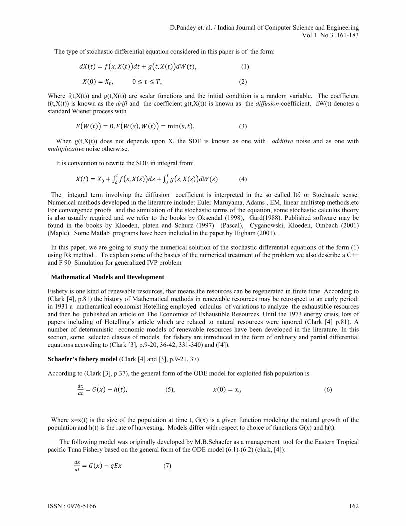
The type of stochastic differential equation considered in this paper is of the form:
, , , (1)
0 , 0 , (2)
Where f(t,X(t)) and g(t,X(t)) are scalar functions and the initial condition is a random variable. The coefficient f(t,X(t)) is known as the drift and the coefficient g(t,X(t)) is known as the diffusion coefficient. dW(t) denotes a standard Wiener process with
0, , min , . (3)
When g(t,X(t)) does not depends upon X, the SDE is known as one with additive noise and as one with multiplicative noise otherwise.
It is convention to rewrite the SDE in integral from:
, , (4)
The integral term involving the diffusion coefficient is interpreted in the so called It or Stochastic sense. Numerical methods developed in the literature include: Euler-Maruyama, Adams , EM, linear multistep methods.etc For convergence proofs and the simulation of the stochastic terms of the equation, some stochastic calculus theory is also usually required and we refer to the books by Oksendal (1998), Gard(1988). Published software may be found in the books by Kloeden, platen and Schurz (1997) (Pascal), Cyganowski, Kloeden, Ombach (2001) (Maple). Some Matlab programs have been included in the paper by Higham (2001).
In this paper, we are going to study the numerical solution of the stochastic differential equations of the form (1) using Rk method . To explain some of the basics of the numerical treatment of the problem we also describe a C++ and F 90 Simulation for generalized IVP problem
Mathematical Models and Development
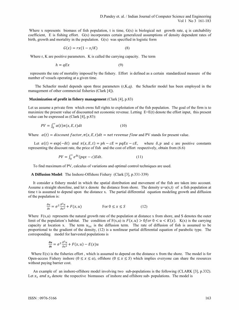
Fishery is one kind of renewable resources, that means the resources can be regenerated in finite time. According to (Clark [4], p.81) the history of Mathematical methods in renewable resources may be retrospect to an early period: in 1931 a mathematical economist Hotelling employed calculus of variations to analyze the exhaustible resources and then he published an article on The Economics of Exhaustible Resources. Until the 1973 energy crisis, lots of papers including of Hotelling’s article which are related to natural resources were ignored (Clark [4] p.81). A number of deterministic economic models of renewable resources have been developed in the literature. In this section, some selected classes of models for fishery are introduced in the form of ordinary and partial differential equations according to (Clark [3], p.9-20, 36-42, 331-340) and ([4]).
Schaefer’s fishery model (Clark [4] and [3], p.9-21, 37)
According to (Clark [3], p.37), the general form of the ODE model for exploited fish population is
, (5), 0 (6)
Where x=x(t) is the size of the population at time t, G(x) is a given function modeling the natural growth of the population and h(t) is the rate of harvesting. Models differ with respect to choice of functions G(x) and h(t).
The following model was originally developed by M.B.Schaefer as a management tool for the Eastern Tropical pacific Tuna Fishery based on the general form of the ODE model (6.1)-(6.2) (clark, [4]):
(7)
ISSN : 0976-5166 162
D.Pandey et. al. / Indian Journal of Computer Science and Engineering Vol 1 No 3 161-183
Where x represents biomass of fish population, t is time, G(x) is biological net growth rate, q is catchability coefficient, E is fishing effort. G(x) incorporates certain generalized assumptions of density dependent rates of birth, growth and mortality in the population. G(x) was specified in logistic form
1 / (8)
Where r, K are positive parameters. K is called the carrying capacity. The term
(9)
represents the rate of mortality imposed by the fishery. Effort is defined as a certain standardized measure of the number of vessels operating at a given time.
The Schaefer model depends upon three parameters (r,K,q). the Schaefer model has been employed in the management of other commercial fisheries (Clark [4]).
Maximization of profit in fishery management (Clark [4], p.83)
Let us assume a private firm which owns full rights to exploitation of the fish population. The goal of the firm is to maximize the present value of discounted net economic revenue. Letting E=E(t) denote the effort input, this present value can be expressed as (Clark [4], p.83):
, ,∞
(10)
Where , , , and PV stands for present value.
Let exp , , , where , and c are positive constants representing the discount rate, the price of fish and the cost of effort respectively, obtain from (6.6)
.∞
(11)
To find maximum of PV, calculus of variations and optimal control techniques are used.
A Diffusion Model: The Inshore-Offshore Fishery (Clark [3], p.331-339)
It consider a fishery model in which the spatial distribution and movement of the fish are taken into account. Assume a straight shoreline, and let x denote the distance from shore. The density u=u(x,t) of a fish population at time t is assumed to depend upon the distance x. The partial differential equation modeling growth and diffusion of the population is:
, For 0 (12)
Where F(x,u) represents the natural growth rate of the population at distance x from shore, and S denotes the outer limit of the population’s habitat. The condition of F(x,u) is , 0 0 . K(x) is the carrying capacity at location x. The term is the diffusion term. The rate of diffusion of fish is assumed to be proportional to the gradient of the density, (12) is a nonlinear partial differential equation of parabolic type. The corresponding model for harvested populations is
,
Where E(x) is the fisheries effort , which is assumed to depend on the distance x from the shore. The model is for Open-access Fishery inshore (0 ), offshore (0 ) which implies everyone can share the resources without paying barrier cost.
An example of an inshore-offshore model involving two sub-populations is the following (CLARK [3], p.332). Let denote the respective biomasses of inshore and offshore sub- populations. The model is
ISSN : 0976-5166 163
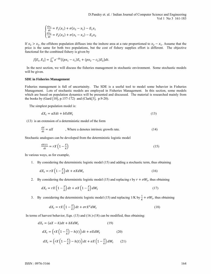
D.Pandey et. al. / Indian Journal of Computer Science and Engineering Vol 1 No 3 161-183
If , the offshore population diffuses into the inshore area at a rate proportioned to . Assume that the price is the same for both two populations, but the cost of fishery supplies effort is different. The objective functional for the combined fishery is given by
, .∞
In the next section, we will discuss the fisheries management in stochastic environment. Some stochastic models will be given.
SDE in Fisheries Management
Fisheries management is full of uncertainity. The SDE is a useful tool to model some behavior in Fisheries Management. Lots of stochastic models are employed in Fisheries Management. In this section, some models which are based on population dynamics will be presented and discussed. The material is researched mainly from the books by (Gard [10], p.157-172) and (Clark[3], p.9-20).
The simplest population model is:
(13)
(13) is an extension of a deterministic model of the form
, Where a denotes intrinsic growth rate. (14)
Stochastic analogues can be developed from the deterministic logistic model
1 (15)
In various ways, as for example,
1. By considering the deterministic logistic model (15) and adding a stochastic term, thus obtaining
1 (16)
2. By considering the deterministic logistic model (15) and replacing r by , thus obtaining
1 1 (17)
3. By considering the deterministic logistic model (15) and replacing 1/K by , thus obtaining
1 (18)
In terms of harvest behavior, Eqn. (13) and (16.)-(18) can be modified, thus obtaining:
(19)
1 (20)
1 1 (21)
ISSN : 0976-5166 164
D.Pandey et. al. / Indian Journal of Computer Science and Engineering Vol 1 No 3 161-183
1 (22)
Numerical results:
In the present study we looking at the numerical solution of the present model. The basic of the paper to simulate the above problem in RKM (Runge kutta Method) scheme using some programming technique. C++ and Fotran-90 being used for it . The two test problem has been introduce for the solution. The analytical result are also presented for the test problems. And comparison being made here in Table-1 to 10. we will provide numerical results which are absolute values of the error at the end point T=1 for different step sizes (∆=1/N). In table 1 to 10, we will also provide ten series of numerical results for ∆=0.0001 (N=1000). In all tables, EM denotes the EM method, Milstein denotes the Milstein mthod, Adams denotes the Adams method with fourth order and RKM (Runge kutta Method)denotes fourth order accurate difference method.
Test problem 1
1 1 (23)
Where 1, 2, 0,1 0.
The exact solution is:
.
The test problem is from (burrage and burrage [2]).
Test problem 2
(24)
Where 0.2246, 4.9028 004, 0.1, 0,1 200000.
The exact solution is:
.
The analytical solution can be derived from (17). the part of coefficients are from (McDonald, Sandal and Steinshamn[21]). Eqn (24) can be employed in fisheries management to model fish population changes in terms of constant harvest.
The numerical results for both cases are showns in tables given below.
Numrical simulation and Grid Generation:
The RKM (Runge kutta Method) has been adopted for the computational solution.. It is vary difficult to give the phenomena of computer programming for all the differential equation our main motivation to simulate over problem using RKM (Runge kutta Method)scheme so a generalized simulation process in C++ and FOTRAN 90 to the simulation algorithm corresponding to the linear differential equation (IVP) taking as counter example is shown here .There are two different kind of scheme can be used for the simplicity on is Implicit and other is semi implicit scheme . The simulation process is given below
FOTRAN
SUBROUTINE DOPRI5(N,FCN,X,Y,XEND, & RTOL,ATOL,ITOL, & SOLOUT,IOUT, & WORK,LWORK,IWORK,LIWORK,RPAR,IPAR,IDID)
C ---------------------------------------------------------- C NUMERICAL SOLUTION OF A SYSTEM OF FIRST 0RDER C ORDINARY DIFFERENTIAL EQUATIONS Y'=F(X,Y). C THIS IS AN EXPLICIT RUNGE-KUTTA METHOD OF ORDER (4)5
ISSN : 0976-5166 165
D.Pandey et. al. / Indian Journal of Computer Science and Engineering Vol 1 No 3 161-183
C DUE TO DORMAND & PRINCE (WITH STEPSIZE CONTROL AND C DENSE OUTPUT). C C C INPUT PARAMETERS C ---------------- C N DIMENSION OF THE SYSTEM C C FCN NAME (EXTERNAL) OF SUBROUTINE COMPUTING THE C VALUE OF F(X,Y): C SUBROUTINE FCN(N,X,Y,F,RPAR,IPAR) C DOUBLE PRECISION X,Y(N),F(N) C F(1)=... ETC. C C X INITIAL X-VALUE C C Y(N) INITIAL VALUES FOR Y C C XEND FINAL X-VALUE (XEND-X MAY BE POSITIVE OR NEGATIVE) C C RTOL,ATOL RELATIVE AND ABSOLUTE ERROR TOLERANCES. THEY C CAN BE BOTH SCALARS OR ELSE BOTH VECTORS OF LENGTH N. C C ITOL SWITCH FOR RTOL AND ATOL: C ITOL=0: BOTH RTOL AND ATOL ARE SCALARS. C THE CODE KEEPS, ROUGHLY, THE LOCAL ERROR OF C Y(I) BELOW RTOL*ABS(Y(I))+ATOL C ITOL=1: BOTH RTOL AND ATOL ARE VECTORS. C THE CODE KEEPS THE LOCAL ERROR OF Y(I) BELOW C RTOL(I)*ABS(Y(I))+ATOL(I). C C SOLOUT NAME (EXTERNAL) OF SUBROUTINE PROVIDING THE C NUMERICAL SOLUTION DURING INTEGRATION. C IF IOUT.GE.1, IT IS CALLED AFTER EVERY SUCCESSFUL STEP. C SUPPLY A DUMMY SUBROUTINE IF IOUT=0. C IT MUST HAVE THE FORM C SUBROUTINE SOLOUT (NR,XOLD,X,Y,N,CON,ICOMP,ND, C RPAR,IPAR,IRTRN) C DIMENSION Y(N),CON(5*ND),ICOMP(ND) C .... C SOLOUT FURNISHES THE SOLUTION "Y" AT THE NR-TH C GRID-POINT "X" (THEREBY THE INITIAL VALUE IS C THE FIRST GRID-POINT). C "XOLD" IS THE PRECEEDING GRID-POINT. C "IRTRN" SERVES TO INTERRUPT THE INTEGRATION. IF IRTRN C IS SET <0, DOPRI5 WILL RETURN TO THE CALLING PROGRAM. C IF THE NUMERICAL SOLUTION IS ALTERED IN SOLOUT, C SET IRTRN = 2 C C ----- CONTINUOUS OUTPUT: ----- C DURING CALLS TO "SOLOUT", A CONTINUOUS SOLUTION
C FOR THE INTERVAL [XOLD,X] IS AVAILABLE THROUGH C THE FUNCTION C >>> CONTD5(I,S,CON,ICOMP,ND) <<< C WHICH PROVIDES AN APPROXIMATION TO THE I-TH C COMPONENT OF THE SOLUTION AT THE POINT S. THE VALUE C S SHOULD LIE IN THE INTERVAL [XOLD,X]. C C IOUT SWITCH FOR CALLING THE SUBROUTINE SOLOUT: C IOUT=0: SUBROUTINE IS NEVER CALLED C IOUT=1: SUBROUTINE IS USED FOR OUTPUT. C IOUT=2: DENSE OUTPUT IS PERFORMED IN SOLOUT C (IN THIS CASE WORK(5) MUST BE SPECIFIED) C C WORK ARRAY OF WORKING SPACE OF LENGTH "LWORK". C WORK(1),...,WORK(20) SERVE AS PARAMETERS FOR THE CODE. C FOR STANDARD USE, SET THEM TO ZERO BEFORE CALLING. C "LWORK" MUST BE AT LEAST 8*N+5*NRDENS+21 C WHERE NRDENS = IWORK(5) C C LWORK DECLARED LENGHT OF ARRAY "WORK". C C IWORK INTEGER WORKING SPACE OF LENGHT "LIWORK". C IWORK(1),...,IWORK(20) SERVE AS PARAMETERS FOR THE CODE. C FOR STANDARD USE, SET THEM TO ZERO BEFORE CALLING. C "LIWORK" MUST BE AT LEAST NRDENS+21 . C C LIWORK DECLARED LENGHT OF ARRAY "IWORK". C C RPAR, IPAR REAL AND INTEGER PARAMETERS (OR PARAMETER ARRAYS) WHICH C CAN BE USED FOR COMMUNICATION BETWEEN YOUR CALLING C PROGRAM AND THE FCN, JAC, MAS, SOLOUT SUBROUTINES. C C----------------------------------------------------------------------- C C SOPHISTICATED SETTING OF PARAMETERS C ----------------------------------- C SEVERAL PARAMETERS (WORK(1),...,IWORK(1),...) ALLOW C TO ADAPT THE CODE TO THE PROBLEM AND TO THE NEEDS OF C THE USER. FOR ZERO INPUT, THE CODE CHOOSES DEFAULT VALUES. C C WORK(1) UROUND, THE ROUNDING UNIT, DEFAULT 2.3D-16. C C WORK(2) THE SAFETY FACTOR IN STEP SIZE PREDICTION, C DEFAULT 0.9D0. C C WORK(3), WORK(4) PARAMETERS FOR STEP SIZE SELECTION C THE NEW STEP SIZE IS CHOSEN SUBJECT TO THE RESTRICTION
ISSN : 0976-5166 166
D.Pandey et. al. / Indian Journal of Computer Science and Engineering Vol 1 No 3 161-183
C WORK(3) <= HNEW/HOLD <= WORK(4) C DEFAULT VALUES: WORK(3)=0.2D0, WORK(4)=10.D0 C C WORK(5) IS THE "BETA" FOR STABILIZED STEP SIZE CONTROL C (SEE SECTION IV.2). LARGER VALUES OF BETA ( <= 0.1 ) C MAKE THE STEP SIZE CONTROL MORE STABLE. DOPRI5 NEEDS C A LARGER BETA THAN HIGHAM & HALL. NEGATIVE WORK(5) C PROVOKE BETA=0. C DEFAULT 0.04D0. C C WORK(6) MAXIMAL STEP SIZE, DEFAULT XEND-X. C C WORK(7) INITIAL STEP SIZE, FOR WORK(7)=0.D0 AN INITIAL GUESS C IS COMPUTED WITH HELP OF THE FUNCTION HINIT C C IWORK(1) THIS IS THE MAXIMAL NUMBER OF ALLOWED STEPS. C THE DEFAULT VALUE (FOR IWORK(1)=0) IS 100000. C C IWORK(2) SWITCH FOR THE CHOICE OF THE COEFFICIENTS C IF IWORK(2).EQ.1 METHOD DOPRI5 OF DORMAND AND PRINCE C (TABLE 5.2 OF SECTION II.5). C AT THE MOMENT THIS IS THE ONLY POSSIBLE CHOICE. C THE DEFAULT VALUE (FOR IWORK(2)=0) IS IWORK(2)=1. C C IWORK(3) SWITCH FOR PRINTING ERROR MESSAGES C IF IWORK(3).LT.0 NO MESSAGES ARE BEING PRINTED C IF IWORK(3).GT.0 MESSAGES ARE PRINTED WITH C WRITE (IWORK(3),*) ... C DEFAULT VALUE (FOR IWORK(3)=0) IS IWORK(3)=6 C C IWORK(4) TEST FOR STIFFNESS IS ACTIVATED AFTER STEP NUMBER C J*IWORK(4) (J INTEGER), PROVIDED IWORK(4).GT.0. C FOR NEGATIVE IWORK(4) THE STIFFNESS TEST IS C NEVER ACTIVATED; DEFAULT VALUE IS IWORK(4)=1000 C C IWORK(5) = NRDENS = NUMBER OF COMPONENTS, FOR WHICH DENSE OUTPUT C IS REQUIRED; DEFAULT VALUE IS IWORK(5)=0; C FOR 0 < NRDENS < N THE COMPONENTS (FOR WHICH DENSE C OUTPUT IS REQUIRED) HAVE TO BE SPECIFIED IN C IWORK(21),...,IWORK(NRDENS+20); C FOR NRDENS=N THIS IS DONE BY THE CODE. C C---------------------------------------------------------------------- C C OUTPUT PARAMETERS C -----------------
C X X-VALUE FOR WHICH THE SOLUTION HAS BEEN COMPUTED C (AFTER SUCCESSFUL RETURN X=XEND). C C Y(N) NUMERICAL SOLUTION AT X C C H PREDICTED STEP SIZE OF THE LAST ACCEPTED STEP C C IDID REPORTS ON SUCCESSFULNESS UPON RETURN: C IDID= 1 COMPUTATION SUCCESSFUL, C IDID= 2 COMPUT. SUCCESSFUL (INTERRUPTED BY SOLOUT) C IDID=-1 INPUT IS NOT CONSISTENT, C IDID=-2 LARGER NMAX IS NEEDED, C IDID=-3 STEP SIZE BECOMES TOO SMALL. C IDID=-4 PROBLEM IS PROBABLY STIFF (INTERRUPTED). C C IWORK(17) NFCN NUMBER OF FUNCTION EVALUATIONS C IWORK(18) NSTEP NUMBER OF COMPUTED STEPS C IWORK(19) NACCPT NUMBER OF ACCEPTED STEPS C IWORK(20) NREJCT NUMBER OF REJECTED STEPS (DUE TO ERROR TEST), C (STEP REJECTIONS IN THE FIRST STEP ARE NOT COUNTED) C----------------------------------------------------------------------- C *** *** *** *** *** *** *** *** *** *** *** *** *** C DECLARATIONS C *** *** *** *** *** *** *** *** *** *** *** *** *** IMPLICIT DOUBLE PRECISION (A-H,O-Z) DIMENSION Y(N),ATOL(*),RTOL(*),WORK(LWORK),IWORK(LIWORK) DIMENSION RPAR(*),IPAR(*) LOGICAL ARRET EXTERNAL FCN,SOLOUT C *** *** *** *** *** *** *** C SETTING THE PARAMETERS C *** *** *** *** *** *** *** NFCN=0 NSTEP=0 NACCPT=0 NREJCT=0 ARRET=.FALSE. C -------- IPRINT FOR MONITORING THE PRINTING IF(IWORK(3).EQ.0)THEN IPRINT=6 ELSE IPRINT=IWORK(3) END IF C -------- NMAX , THE MAXIMAL NUMBER OF STEPS ----- IF(IWORK(1).EQ.0)THEN NMAX=100000 ELSE NMAX=IWORK(1) IF(NMAX.LE.0)THEN IF (IPRINT.GT.0) WRITE(IPRINT,*) & ' WRONG INPUT IWORK(1)=',IWORK(1) ARRET=.TRUE. END IF END IF C -------- METH COEFFICIENTS OF THE METHOD IF(IWORK(2).EQ.0)THEN METH=1 ELSE METH=IWORK(2) IF(METH.LE.0.OR.METH.GE.4)THEN IF (IPRINT.GT.0) WRITE(IPRINT,*)
ISSN : 0976-5166 167

D.Pandey et. al. / Indian Journal of Computer Science and Engineering Vol 1 No 3 161-183
& ' CURIOUS INPUT IWORK(2)=',IWORK(2) ARRET=.TRUE. END IF END IF C -------- NSTIFF PARAMETER FOR STIFFNESS DETECTION NSTIFF=IWORK(4) IF (NSTIFF.EQ.0) NSTIFF=1000 IF (NSTIFF.LT.0) NSTIFF=NMAX+10 C -------- NRDENS NUMBER OF DENSE OUTPUT COMPONENTS NRDENS=IWORK(5) IF(NRDENS.LT.0.OR.NRDENS.GT.N)THEN IF (IPRINT.GT.0) WRITE(IPRINT,*) & ' CURIOUS INPUT IWORK(5)=',IWORK(5) ARRET=.TRUE. ELSE IF(NRDENS.GT.0.AND.IOUT.LT.2)THEN IF (IPRINT.GT.0) WRITE(IPRINT,*) & ' WARNING: PUT IOUT=2 FOR DENSE OUTPUT ' END IF IF (NRDENS.EQ.N) THEN DO 16 I=1,NRDENS 16 IWORK(20+I)=I END IF END IF C -------- UROUND SMALLEST NUMBER SATISFYING 1.D0+UROUND>1.D0 IF(WORK(1).EQ.0.D0)THEN UROUND=2.3D-16 ELSE UROUND=WORK(1) IF(UROUND.LE.1.D-35.OR.UROUND.GE.1.D0)THEN IF (IPRINT.GT.0) WRITE(IPRINT,*) & ' WHICH MACHINE DO YOU HAVE? YOUR UROUND WAS:',WORK(1) ARRET=.TRUE. END IF END IF C ------- SAFETY FACTOR ------------- IF(WORK(2).EQ.0.D0)THEN SAFE=0.9D0 ELSE SAFE=WORK(2) IF(SAFE.GE.1.D0.OR.SAFE.LE.1.D-4)THEN IF (IPRINT.GT.0) WRITE(IPRINT,*) & ' CURIOUS INPUT FOR SAFETY FACTOR WORK(2)=',WORK(2) ARRET=.TRUE. END IF END IF C ------- FAC1,FAC2 PARAMETERS FOR STEP SIZE SELECTION IF(WORK(3).EQ.0.D0)THEN FAC1=0.2D0 ELSE FAC1=WORK(3) END IF IF(WORK(4).EQ.0.D0)THEN FAC2=10.D0 ELSE FAC2=WORK(4) END IF C --------- BETA FOR STEP CONTROL STABILIZATION ----------- IF(WORK(5).EQ.0.D0)THEN BETA=0.04D0 ELSE IF(WORK(5).LT.0.D0)THEN BETA=0.D0
ELSE BETA=WORK(5) IF(BETA.GT.0.2D0)THEN IF (IPRINT.GT.0) WRITE(IPRINT,*) & ' CURIOUS INPUT FOR BETA: WORK(5)=',WORK(5) ARRET=.TRUE. END IF END IF END IF C -------- MAXIMAL STEP SIZE IF(WORK(6).EQ.0.D0)THEN HMAX=XEND-X ELSE HMAX=WORK(6) END IF C -------- INITIAL STEP SIZE H=WORK(7) C ------- PREPARE THE ENTRY-POINTS FOR THE ARRAYS IN WORK ----- IEY1=21 IEK1=IEY1+N IEK2=IEK1+N IEK3=IEK2+N IEK4=IEK3+N IEK5=IEK4+N IEK6=IEK5+N IEYS=IEK6+N IECO=IEYS+N C ------ TOTAL STORAGE REQUIREMENT ----------- ISTORE=IEYS+5*NRDENS-1 IF(ISTORE.GT.LWORK)THEN IF (IPRINT.GT.0) WRITE(IPRINT,*) & ' INSUFFICIENT STORAGE FOR WORK, MIN. LWORK=',ISTORE ARRET=.TRUE. END IF ICOMP=21 ISTORE=ICOMP+NRDENS-1 IF(ISTORE.GT.LIWORK)THEN IF (IPRINT.GT.0) WRITE(IPRINT,*) & ' INSUFFICIENT STORAGE FOR IWORK, MIN. LIWORK=',ISTORE ARRET=.TRUE. END IF C ------ WHEN A FAIL HAS OCCURED, WE RETURN WITH IDID=-1 IF (ARRET) THEN IDID=-1 RETURN END IF C -------- CALL TO CORE INTEGRATOR ------------ CALL DOPCOR(N,FCN,X,Y,XEND,HMAX,H,RTOL,ATOL,ITOL,IPRINT, & SOLOUT,IOUT,IDID,NMAX,UROUND,METH,NSTIFF,SAFE,BETA,FAC1,FAC2, & WORK(IEY1),WORK(IEK1),WORK(IEK2),WORK(IEK3),WORK(IEK4), & WORK(IEK5),WORK(IEK6),WORK(IEYS),WORK(IECO),IWORK(ICOMP), & NRDENS,RPAR,IPAR,NFCN,NSTEP,NACCPT,NREJCT) WORK(7)=H IWORK(17)=NFCN IWORK(18)=NSTEP IWORK(19)=NACCPT IWORK(20)=NREJCT
ISSN : 0976-5166 168

D.Pandey et. al. / Indian Journal of Computer Science and Engineering Vol 1 No 3 161-183
C ----------- RETURN ----------- RETURN END C C C C ----- ... AND HERE IS THE CORE INTEGRATOR ---------- C SUBROUTINE DOPCOR(N,FCN,X,Y,XEND,HMAX,H,RTOL,ATOL,ITOL,IPRINT, & SOLOUT,IOUT,IDID,NMAX,UROUND,METH,NSTIFF,SAFE,BETA,FAC1,FAC2, & Y1,K1,K2,K3,K4,K5,K6,YSTI,CONT,ICOMP,NRD,RPAR,IPAR, & NFCN,NSTEP,NACCPT,NREJCT) C ---------------------------------------------------------- C CORE INTEGRATOR FOR DOPRI5 C PARAMETERS SAME AS IN DOPRI5 WITH WORKSPACE ADDED C ---------------------------------------------------------- C DECLARATIONS C ---------------------------------------------------------- IMPLICIT DOUBLE PRECISION (A-H,O-Z) DOUBLE PRECISION K1(N),K2(N),K3(N),K4(N),K5(N),K6(N) DIMENSION Y(N),Y1(N),YSTI(N),ATOL(*),RTOL(*),RPAR(*),IPAR(*) DIMENSION CONT(5*NRD),ICOMP(NRD) LOGICAL REJECT,LAST EXTERNAL FCN COMMON /CONDO5/XOLD,HOUT C *** *** *** *** *** *** *** C INITIALISATIONS C *** *** *** *** *** *** *** IF (METH.EQ.1) CALL CDOPRI(C2,C3,C4,C5,E1,E3,E4,E5,E6,E7, & A21,A31,A32,A41,A42,A43,A51,A52,A53,A54, & A61,A62,A63,A64,A65,A71,A73,A74,A75,A76, & D1,D3,D4,D5,D6,D7) FACOLD=1.D-4 EXPO1=0.2D0-BETA*0.75D0 FACC1=1.D0/FAC1 FACC2=1.D0/FAC2 POSNEG=SIGN(1.D0,XEND-X) C --- INITIAL PREPARATIONS ATOLI=ATOL(1) RTOLI=RTOL(1) LAST=.FALSE. HLAMB=0.D0 IASTI=0 CALL FCN(N,X,Y,K1,RPAR,IPAR) HMAX=ABS(HMAX) IORD=5 IF (H.EQ.0.D0) H=HINIT(N,FCN,X,Y,XEND,POSNEG,K1,K2,K3,IORD, & HMAX,ATOL,RTOL,ITOL,RPAR,IPAR) NFCN=NFCN+2 REJECT=.FALSE. XOLD=X IF (IOUT.NE.0) THEN IRTRN=1 HOUT=H CALL SOLOUT(NACCPT+1,XOLD,X,Y,N,CONT,ICOMP,NRD, & RPAR,IPAR,IRTRN) IF (IRTRN.LT.0) GOTO 79 ELSE IRTRN=0
END IF C --- BASIC INTEGRATION STEP 1 CONTINUE IF (NSTEP.GT.NMAX) GOTO 78 IF (0.1D0*ABS(H).LE.ABS(X)*UROUND)GOTO 77 IF ((X+1.01D0*H-XEND)*POSNEG.GT.0.D0) THEN H=XEND-X LAST=.TRUE. END IF NSTEP=NSTEP+1 C --- THE FIRST 6 STAGES IF (IRTRN.GE.2) THEN CALL FCN(N,X,Y,K1,RPAR,IPAR) END IF DO 22 I=1,N 22 Y1(I)=Y(I)+H*A21*K1(I) CALL FCN(N,X+C2*H,Y1,K2,RPAR,IPAR) DO 23 I=1,N 23 Y1(I)=Y(I)+H*(A31*K1(I)+A32*K2(I)) CALL FCN(N,X+C3*H,Y1,K3,RPAR,IPAR) DO 24 I=1,N 24 Y1(I)=Y(I)+H*(A41*K1(I)+A42*K2(I)+A43*K3(I)) CALL FCN(N,X+C4*H,Y1,K4,RPAR,IPAR) DO 25 I=1,N 25 Y1(I)=Y(I)+H*(A51*K1(I)+A52*K2(I)+A53*K3(I)+A54*K4(I)) CALL FCN(N,X+C5*H,Y1,K5,RPAR,IPAR) DO 26 I=1,N 26 YSTI(I)=Y(I)+H*(A61*K1(I)+A62*K2(I)+A63*K3(I)+A64*K4(I)+A65*K5(I)) XPH=X+H CALL FCN(N,XPH,YSTI,K6,RPAR,IPAR) DO 27 I=1,N 27 Y1(I)=Y(I)+H*(A71*K1(I)+A73*K3(I)+A74*K4(I)+A75*K5(I)+A76*K6(I)) CALL FCN(N,XPH,Y1,K2,RPAR,IPAR) IF (IOUT.GE.2) THEN DO 40 J=1,NRD I=ICOMP(J) CONT(4*NRD+J)=H*(D1*K1(I)+D3*K3(I)+D4*K4(I)+D5*K5(I) & +D6*K6(I)+D7*K2(I)) 40 CONTINUE END IF DO 28 I=1,N 28 K4(I)=(E1*K1(I)+E3*K3(I)+E4*K4(I)+E5*K5(I)+E6*K6(I)+E7*K2(I))*H NFCN=NFCN+6 C --- ERROR ESTIMATION ERR=0.D0 IF (ITOL.EQ.0) THEN DO 41 I=1,N SK=ATOLI+RTOLI*MAX(ABS(Y(I)),ABS(Y1(I))) 41 ERR=ERR+(K4(I)/SK)**2 ELSE DO 42 I=1,N SK=ATOL(I)+RTOL(I)*MAX(ABS(Y(I)),ABS(Y1(I))) 42 ERR=ERR+(K4(I)/SK)**2 END IF ERR=SQRT(ERR/N) C --- COMPUTATION OF HNEW FAC11=ERR**EXPO1 C --- LUND-STABILIZATION FAC=FAC11/FACOLD**BETA C --- WE REQUIRE FAC1 <= HNEW/H <= FAC2 FAC=MAX(FACC2,MIN(FACC1,FAC/SAFE))
ISSN : 0976-5166 169
D.Pandey et. al. / Indian Journal of Computer Science and Engineering Vol 1 No 3 161-183
HNEW=H/FAC IF(ERR.LE.1.D0)THEN C --- STEP IS ACCEPTED FACOLD=MAX(ERR,1.0D-4) NACCPT=NACCPT+1 C ------- STIFFNESS DETECTION IF (MOD(NACCPT,NSTIFF).EQ.0.OR.IASTI.GT.0) THEN STNUM=0.D0 STDEN=0.D0 DO 64 I=1,N STNUM=STNUM+(K2(I)-K6(I))**2 STDEN=STDEN+(Y1(I)-YSTI(I))**2 64 CONTINUE IF (STDEN.GT.0.D0) HLAMB=H*SQRT(STNUM/STDEN) IF (HLAMB.GT.3.25D0) THEN NONSTI=0 IASTI=IASTI+1 IF (IASTI.EQ.15) THEN IF (IPRINT.GT.0) WRITE (IPRINT,*) & ' THE PROBLEM SEEMS TO BECOME STIFF AT X = ',X IF (IPRINT.LE.0) GOTO 76 END IF ELSE NONSTI=NONSTI+1 IF (NONSTI.EQ.6) IASTI=0 END IF END IF IF (IOUT.GE.2) THEN DO 43 J=1,NRD I=ICOMP(J) YD0=Y(I) YDIFF=Y1(I)-YD0 BSPL=H*K1(I)-YDIFF CONT(J)=Y(I) CONT(NRD+J)=YDIFF CONT(2*NRD+J)=BSPL CONT(3*NRD+J)=-H*K2(I)+YDIFF-BSPL 43 CONTINUE END IF DO 44 I=1,N K1(I)=K2(I) 44 Y(I)=Y1(I) XOLD=X X=XPH IF (IOUT.NE.0) THEN HOUT=H CALL SOLOUT(NACCPT+1,XOLD,X,Y,N,CONT,ICOMP,NRD, & RPAR,IPAR,IRTRN) IF (IRTRN.LT.0) GOTO 79 END IF C ------- NORMAL EXIT IF (LAST) THEN H=HNEW IDID=1 RETURN END IF IF(ABS(HNEW).GT.HMAX)HNEW=POSNEG*HMAX IF(REJECT)HNEW=POSNEG*MIN(ABS(HNEW),ABS(H)) REJECT=.FALSE. ELSE C --- STEP IS REJECTED HNEW=H/MIN(FACC1,FAC11/SAFE) REJECT=.TRUE. IF(NACCPT.GE.1)NREJCT=NREJCT+1 LAST=.FALSE. END IF
H=HNEW GOTO 1 C --- FAIL EXIT 76 CONTINUE IDID=-4 RETURN 77 CONTINUE IF (IPRINT.GT.0) WRITE(IPRINT,979)X IF (IPRINT.GT.0) WRITE(IPRINT,*)' STEP SIZE T0O SMALL, H=',H IDID=-3 RETURN 78 CONTINUE IF (IPRINT.GT.0) WRITE(IPRINT,979)X IF (IPRINT.GT.0) WRITE(IPRINT,*) & ' MORE THAN NMAX =',NMAX,'STEPS ARE NEEDED' IDID=-2 RETURN 79 CONTINUE IF (IPRINT.GT.0) WRITE(IPRINT,979)X 979 FORMAT(' EXIT OF DOPRI5 AT X=',E18.4) IDID=2 RETURN END C FUNCTION HINIT(N,FCN,X,Y,XEND,POSNEG,F0,F1,Y1,IORD, & HMAX,ATOL,RTOL,ITOL,RPAR,IPAR) C ---------------------------------------------------------- C ---- COMPUTATION OF AN INITIAL STEP SIZE GUESS C ---------------------------------------------------------- IMPLICIT DOUBLE PRECISION (A-H,O-Z) DIMENSION Y(N),Y1(N),F0(N),F1(N),ATOL(*),RTOL(*) DIMENSION RPAR(*),IPAR(*) C ---- COMPUTE A FIRST GUESS FOR EXPLICIT EULER AS C ---- H = 0.01 * NORM (Y0) / NORM (F0) C ---- THE INCREMENT FOR EXPLICIT EULER IS SMALL C ---- COMPARED TO THE SOLUTION DNF=0.0D0 DNY=0.0D0 ATOLI=ATOL(1) RTOLI=RTOL(1) IF (ITOL.EQ.0) THEN DO 10 I=1,N SK=ATOLI+RTOLI*ABS(Y(I)) DNF=DNF+(F0(I)/SK)**2 10 DNY=DNY+(Y(I)/SK)**2 ELSE DO 11 I=1,N SK=ATOL(I)+RTOL(I)*ABS(Y(I)) DNF=DNF+(F0(I)/SK)**2 11 DNY=DNY+(Y(I)/SK)**2 END IF IF (DNF.LE.1.D-10.OR.DNY.LE.1.D-10) THEN H=1.0D-6 ELSE H=SQRT(DNY/DNF)*0.01D0 END IF H=MIN(H,HMAX) H=SIGN(H,POSNEG) C ---- PERFORM AN EXPLICIT EULER STEP DO 12 I=1,N 12 Y1(I)=Y(I)+H*F0(I) CALL FCN(N,X+H,Y1,F1,RPAR,IPAR) C ---- ESTIMATE THE SECOND DERIVATIVE OF THE SOLUTION DER2=0.0D0 IF (ITOL.EQ.0) THEN DO 15 I=1,N
ISSN : 0976-5166 170

D.Pandey et. al. / Indian Journal of Computer Science and Engineering Vol 1 No 3 161-183
SK=ATOLI+RTOLI*ABS(Y(I)) 15 DER2=DER2+((F1(I)-F0(I))/SK)**2 ELSE DO 16 I=1,N SK=ATOL(I)+RTOL(I)*ABS(Y(I)) 16 DER2=DER2+((F1(I)-F0(I))/SK)**2 END IF DER2=SQRT(DER2)/H C ---- STEP SIZE IS COMPUTED SUCH THAT C ---- H**IORD * MAX ( NORM (F0), NORM (DER2)) = 0.01 DER12=MAX(ABS(DER2),SQRT(DNF)) IF (DER12.LE.1.D-15) THEN H1=MAX(1.0D-6,ABS(H)*1.0D-3) ELSE H1=(0.01D0/DER12)**(1.D0/IORD) END IF H=MIN(100*ABS(H),H1,HMAX) HINIT=SIGN(H,POSNEG) RETURN END C FUNCTION CONTD5(II,X,CON,ICOMP,ND) C ---------------------------------------------------------- C THIS FUNCTION CAN BE USED FOR CONTINUOUS OUTPUT IN CONNECTION C WITH THE OUTPUT-SUBROUTINE FOR DOPRI5. IT PROVIDES AN C APPROXIMATION TO THE II-TH COMPONENT OF THE SOLUTION AT X. C ---------------------------------------------------------- IMPLICIT DOUBLE PRECISION (A-H,O-Z) DIMENSION CON(5*ND),ICOMP(ND) COMMON /CONDO5/XOLD,H C ----- COMPUTE PLACE OF II-TH COMPONENT I=0 DO 5 J=1,ND IF (ICOMP(J).EQ.II) I=J 5 CONTINUE IF (I.EQ.0) THEN WRITE (6,*) ' NO DENSE OUTPUT AVAILABLE FOR COMP.',II RETURN END IF THETA=(X-XOLD)/H THETA1=1.D0-THETA CONTD5=CON(I)+THETA*(CON(ND+I)+THETA1*(CON(2*ND+I)+THETA* & (CON(3*ND+I)+THETA1*CON(4*ND+I)))) RETURN END C SUBROUTINE CDOPRI(C2,C3,C4,C5,E1,E3,E4,E5,E6,E7, & A21,A31,A32,A41,A42,A43,A51,A52,A53,A54, & A61,A62,A63,A64,A65,A71,A73,A74,A75,A76, & D1,D3,D4,D5,D6,D7) C ---------------------------------------------------------- C RUNGE-KUTTA COEFFICIENTS OF DORMAND AND PRINCE (1980) C ---------------------------------------------------------- IMPLICIT DOUBLE PRECISION (A-H,O-Z) C2=0.2D0 C3=0.3D0 C4=0.8D0 C5=8.D0/9.D0 A21=0.2D0 A31=3.D0/40.D0 A32=9.D0/40.D0 A41=44.D0/45.D0 A42=-56.D0/15.D0
A43=32.D0/9.D0 A51=19372.D0/6561.D0 A52=-25360.D0/2187.D0 A53=64448.D0/6561.D0 A54=-212.D0/729.D0 A61=9017.D0/3168.D0 A62=-355.D0/33.D0 A63=46732.D0/5247.D0 A64=49.D0/176.D0 A65=-5103.D0/18656.D0 A71=35.D0/384.D0 A73=500.D0/1113.D0 A74=125.D0/192.D0 A75=-2187.D0/6784.D0 A76=11.D0/84.D0 E1=71.D0/57600.D0 E3=-71.D0/16695.D0 E4=71.D0/1920.D0 E5=-17253.D0/339200.D0 E6=22.D0/525.D0 E7=-1.D0/40.D0 C ---- DENSE OUTPUT OF SHAMPINE (1986) D1=-12715105075.D0/11282082432.D0 D3=87487479700.D0/32700410799.D0 D4=-10690763975.D0/1880347072.D0 D5=701980252875.D0/199316789632.D0 D6=-1453857185.D0/822651844.D0 D7=69997945.D0/29380423.D0 RETURN END
/*************************************************************************/
A C++ Program to estimate the Differential value of a given
function at given point from given data using Runge-Kutta Methods.
******************************************************
//--------------------------- Header Files ----------------------------//
****************************************************** # include <iostream.h>
# include <stdlib.h>
# include <string.h>
# include <stdio.h>
# include <conio.h>
# include <math.h>
/*****************************************************
//------------------------ Global Variables ---------------------------//
/*****************************************************
ISSN : 0976-5166 171
D.Pandey et. al. / Indian Journal of Computer Science and Engineering Vol 1 No 3 161-183
const int max_size=13;
int n=0;
int top=-1;
long double h=0;
long double x=0;
long double x0=0;
long double y0=0;
long double two_stage_result=0;
long double three_stage_result=0;
long double xx[max_size]={0};
long double yy2[max_size]={0};
long double yy3[max_size]={0};
char Fx[100]={NULL};
char Stack[30][30]={NULL};
char Postfix_expression[30][30]={NULL};
/***************************************************** //------------------------ Funcion Prototypes -------------------------//
/*****************************************************
void push(const char *);
void convert_ie_to_pe(const char *);
const char* pop( );
const long double evaluate_pe(const long double,const long double);
void show_screen( );
void clear_screen( );
void get_input( );
void apply_runge_kutta_method( );
void show_result( );
/*****************************************************
//------------------------------ main( ) ------------------------------//
/*****************************************************
int main( ) {
clrscr( );
textmode(C4350);
show_screen( );
get_input( );
apply_runge_kutta_method( );
show_result( );
getch( );
return 0;
}
/*****************************************************
//------------------------ Funcion Definitions ------------------------//
***************************************************
//-------------------------- show_screen( ) ---------------------------//
********************/
void show_screen( )
{
cprintf("\n******************************************");
cprintf("***************************- ");
cprintf("*--------------------------- ");
textbackground(1);
cprintf(" Numerical Integration ");
textbackground(8);
cprintf(" --------------------------*");
cprintf("*-*************************- -*");
cprintf("*********************************-*");
for(int count=0;count<42;count++)
cprintf("*-* *-*");
gotoxy(1,46);
cprintf("**********************************-*");
cprintf("*------------------------------------------------------------------------------*");
cprintf("*****************************************");
gotoxy(1,2);
}
ISSN : 0976-5166 172

D.Pandey et. al. / Indian Journal of Computer Science and Engineering Vol 1 No 3 161-183
******************************************************
//------------------------- clear_screen( ) ---------------------------//
********************/
void clear_screen( )
{
for(int count=0;count<37;count++)
{
gotoxy(5,8+count);
cout<<" ";
}
gotoxy(1,2);
}
********************/
//-------------------------- push(const char*) ------------------------//
/***************************************************** void push(const char* Operand)
{
if(top==(max_size-1))
{
cout<<"Error : Stack is full."<<endl;
cout<<"\n Press any key to exit.";
getch( );
exit(0);
}
else
{
top++;
strcpy(Stack[top],Operand);
}
}
/*****************************************************
//------------------------------ pop( ) -------------------------------//
/*****************************************************
const char* pop( )
{
char Operand[40]={NULL};
if(top==-1)
{
cout<<"Error : Stack is empty."<<endl;
cout<<"\n Press any key to exit.";
getch( );
exit(0);
}
else
{
strcpy(Operand,Stack[top]);
strset(Stack[top],NULL);
top--;
}
return Operand;
}
/*****************************************************
//-------------------- convert_ie_to_pe(const char*) ------------------
/*****************************************************
void convert_ie_to_pe(const char* Expression)
{
char Infix_expression[100]={NULL};
char Symbol_scanned[30]={NULL};
push("(");
strcpy(Infix_expression,Expression);
strcat(Infix_expression,"+0)");
int flag=0;
int count_1=0;
int count_2=0;
ISSN : 0976-5166 173

D.Pandey et. al. / Indian Journal of Computer Science and Engineering Vol 1 No 3 161-183
int equation_length=strlen(Infix_expression);
if(Infix_expression[0]=='(')
flag=1;
do
{
strset(Symbol_scanned,NULL);
if(flag==0)
{
int count_3=0;
do
{
Symbol_scanned[count_3]=Infix_expression[count_1];
count_1++;
count_3++;
}
while(count_1<=equation_length &&
Infix_expression[count_1]!='(' &&
Infix_expression[count_1]!='+' &&
Infix_expression[count_1]!='-' &&
Infix_expression[count_1]!='*' &&
Infix_expression[count_1]!='/' &&
Infix_expression[count_1]!='^' &&
Infix_expression[count_1]!=')');
flag=1;
}
else if(flag==1)
{
Symbol_scanned[0]=Infix_expression[count_1];
count_1++;
if(Infix_expression[count_1]!='(' &&
Infix_expression[count_1]!='^' &&
Infix_expression[count_1]!='*' &&
Infix_expression[count_1]!='/' &&
Infix_expression[count_1]!='+' &&
Infix_expression[count_1]!='-' &&
Infix_expression[count_1]!=')')
flag=0;
if(Infix_expression[count_1-1]=='(' &&
(Infix_expression[count_1]=='-' ||
Infix_expression[count_1]=='+'))
flag=0;
}
if(strcmp(Symbol_scanned,"(")==0)
push("(");
else if(strcmp(Symbol_scanned,")")==0)
{
while(strcmp(Stack[top],"(")!=0)
{
strcpy(Postfix_expression[count_2],pop( ));
count_2++;
}
pop( );
}
else if(strcmp(Symbol_scanned,"^")==0 ||
ISSN : 0976-5166 174

D.Pandey et. al. / Indian Journal of Computer Science and Engineering Vol 1 No 3 161-183
strcmp(Symbol_scanned,"+")==0 ||
strcmp(Symbol_scanned,"-")==0 ||
strcmp(Symbol_scanned,"*")==0 ||
strcmp(Symbol_scanned,"/")==0)
{
if(strcmp(Symbol_scanned,"^")==0)
{ }
else if(strcmp(Symbol_scanned,"*")==0 ||
strcmp(Symbol_scanned,"/")==0)
{
while(strcmp(Stack[top],"^")==0 ||
strcmp(Stack[top],"*")==0 ||
strcmp(Stack[top],"/")==0)
{
strcpy(Postfix_expression[count_2],pop( ));
count_2++;
}
}
else if(strcmp(Symbol_scanned,"+")==0 ||
strcmp(Symbol_scanned,"-")==0)
{
while(strcmp(Stack[top],"(")!=0)
{
strcpy(Postfix_expression[count_2],pop( ));
count_2++;
} }
push(Symbol_scanned);
}
else
{
strcat(Postfix_expression[count_2],Symbol_scanned);
count_2++;
} }
while(strcmp(Stack[top],NULL)!=0);
strcat(Postfix_expression[count_2],"=");
count_2++;
}
/*****************************************************
//---------- evaluate_pe(const long double,const long double) -----/
/*****************************************************
const long double evaluate_pe(const long double x,const long double y)
{
long double function_value=0;
int count_1=-1;
char Symbol_scanned[30]={NULL};
do
{
count_1++;
strcpy(Symbol_scanned,Postfix_expression[count_1]);
if(strcmp(Symbol_scanned,"^")==0 ||
strcmp(Symbol_scanned,"*")==0 ||
strcmp(Symbol_scanned,"/")==0 ||
strcmp(Symbol_scanned,"+")==0 ||
strcmp(Symbol_scanned,"-")==0)
{
char Result[30]={NULL};
char Operand[2][30]={NULL};
strcpy(Operand[0],pop( ));
strcpy(Operand[1],pop( ));
long double operand[2]={0};
ISSN : 0976-5166 175

D.Pandey et. al. / Indian Journal of Computer Science and Engineering Vol 1 No 3 161-183
long double result=0;
char *endptr;
for(int count_2=0;count_2<2;count_2++)
{
int flag=0;
if(Operand[count_2][0]=='-')
{
int length=strlen(Operand[count_2]);
for(int count_3=0;count_3<(length-1);count_3++)
Operand[count_2][count_3]=Operand[count_2][(count_3+1)];
Operand[count_2][count_3]=NULL;
flag=1;
}
if(strcmp(Operand[count_2],"x")==0)
operand[count_2]=x;
else if(strcmp(Operand[count_2],"y")==0)
operand[count_2]=y;
else if(strcmp(Operand[count_2],"e")==0)
operand[count_2]=2.718282;
else if(strcmp(Operand[count_2],"sinx")==0)
operand[count_2]=sinl(x);
else if(strcmp(Operand[count_2],"cosx")==0)
operand[count_2]=cosl(x);
else if(strcmp(Operand[count_2],"tanx")==0)
operand[count_2]=tanl(x);
else if(strcmp(Operand[count_2],"lnx")==0)
operand[count_2]=logl(x);
else if(strcmp(Operand[count_2],"logx")==0)
operand[count_2]=log10l(x);
else if(strcmp(Operand[count_2],"siny")==0)
operand[count_2]=sinl(y);
else if(strcmp(Operand[count_2],"cosy")==0)
operand[count_2]=cosl(y);
else if(strcmp(Operand[count_2],"tany")==0)
operand[count_2]=tanl(y);
else if(strcmp(Operand[count_2],"lny")==0)
operand[count_2]=logl(y);
else if(strcmp(Operand[count_2],"logy")==0)
operand[count_2]=log10l(y);
else
operand[count_2]=strtod(Operand[count_2],&endptr);
if(flag)
operand[count_2]*=-1;
}
switch(Symbol_scanned[0])
{
case '^' : result=powl(operand[1],operand[0]);
break;
case '*' : result=operand[1]*operand[0];
break;
case '/' : result=operand[1]/operand[0];
break;
case '+' : result=operand[1]+operand[0];
break;
case '-' : result=operand[1]-operand[0];
break;
}
gcvt(result,25,Result);
ISSN : 0976-5166 176

D.Pandey et. al. / Indian Journal of Computer Science and Engineering Vol 1 No 3 161-183
push(Result);
}
else if(strcmp(Symbol_scanned,"=")!=0)
push(Symbol_scanned);
}
while(strcmp(Symbol_scanned,"=")!=0);
char Function_value[30]={NULL};
char *endptr;
strcpy(Function_value,pop( ));
function_value=strtod(Function_value,&endptr);
return function_value;
}
*****************************************************
//----------------------------- get_input( ) --------------------------//
******************************************************
void get_input( )
{
clear_screen( );
gotoxy(6,10);
cout<<"Input :";
gotoxy(6,11);
cout<<"ÍÍÍÍÍÍÍ";
gotoxy(6,37);
cout<<"Note : Write the function with proper Braces ( ) e.g; 2x+3 as (2*x)+3";
gotoxy(6,40);
cout<<"Available Operators : ^ (raised to power) , * , / , + , -";
gotoxy(6,42);
cout<<"Available Operands : x , e , sinx , cosx , tanx , lnx , logx ,";
gotoxy(6,44);
cout<<" any number and all above functions with y.";
gotoxy(6,14);
cout<<"Enter the Function : f(x,y) = ";
cin>>Fx;
convert_ie_to_pe(Fx);
gotoxy(6,17);
cout<<"Enter the value of xn = ";
cin>>x;
gotoxy(6,19);
cout<<"Enter the value of x0 = ";
cin>>x0;
gotoxy(6,21);
cout<<"Enter the value of y0 = ";
cin>>y0;
gotoxy(6,23);
cout<<"Enter the value of h = ";
cin>>h;
}
/***************************************************** //-------------------- apply_ruunge_kutta_method( ) -------------------
******************************************************
void apply_runge_kutta_method( )
{
xx[0]=x0;
yy2[0]=y0;
yy3[0]=y0;
do
{
xx[(n+1)]=(xx[n]+h);
n++;
}
while(xx[n]<x);
long double k1=0;
long double k2=0;
long double ynp1=0;
long double xn=x0;
ISSN : 0976-5166 177
D.Pandey et. al. / Indian Journal of Computer Science and Engineering Vol 1 No 3 161-183
long double yn=y0;
for(int count_1=0;count_1<n;count_1++)
{
k1=0;
k2=0;
ynp1=0;
k1=evaluate_pe(xn,yn);
k2=evaluate_pe((xn+h),(yn+(h*k1)));
ynp1=(yn+((h*(k1+k2))/2));
yn=ynp1;
xn+=h;
yy2[(count_1+1)]=ynp1;
}
two_stage_result=ynp1;
long double k3=0;
long double k4=0;
xn=x0;
yn=y0;
for(int count_2=0;count_2<n;count_2++)
{
k1=0;
k2=0;
k3=0;
k4=0;
ynp1=0;
k1=evaluate_pe(xn,yn);
k2=evaluate_pe((xn+(h/2)),(yn+((h*k1)/2)));
k3=evaluate_pe((xn+(h/2)),(yn+((h*k2)/2)));
k4=evaluate_pe((xn+h),(yn+(h*k3)));
ynp1=(yn+((h*(k1+(2*k2)+(2*k3)+k4))/6));
yn=ynp1;
xn+=h;
yy3[(count_2+1)]=ynp1;
}
three_stage_result=ynp1;
clear_screen( );
gotoxy(6,9);
cout<<"Solution :";
gotoxy(6,10);
cout<<"ÍÍÍÍÍÍÍÍÍÍ";
gotoxy(18,12);
cout<<"ÚÄÄÄÄÄÄÄÄÄÄÄÄÄÄÄÂÄÄ¿";
gotoxy(18,13);
cout<<"³ x ³ 2-stage y ³ 3-stage y ³";
gotoxy(18,14);
cout<<"ÃÄÄÄÄÄÄÄÄÄÄÄÄÄÄÄÅÄÄÄÄÄ´";
gotoxy(18,15);
cout<<"³ ³ ³ ³";
for(int count_3=0;count_3<=n;count_3++)
{
gotoxy(18,(wherey( )+1));
cout<<"³ ³ ³ ³";
gotoxy(18,(wherey( )+1));
cout<<"³ ³ ³ ³";
}
gotoxy(18,(wherey( )+1));
cout<<"ÀÄÄÄÄÄÄÄÄÄÄÄÄÄÄÄÁÄÄÄÄÄ
gotoxy(25,16);
for(int count_4=0;count_4<=n;count_4++)
{
gotoxy(20,wherey( ));
cout<<xx[count_4];
gotoxy(36,wherey( ));
cout<<yy2[count_4];
gotoxy(52,wherey( ));
cout<<yy3[count_4];
gotoxy(25,(wherey( )+2));
ISSN : 0976-5166 178

D.Pandey et. al. / Indian Journal of Computer Science and Engineering Vol 1 No 3 161-183
}
gotoxy(25,43);
cout<<"Press any key to continue...";
getch( );
}
/*************************************************************************/
//---------------------------- show_result( ) -------------------------//
/************************************************************************/
void show_result( )
{
clear_screen( );
gotoxy(6,9);
cout<<"Runge-Kutta Methods :";
gotoxy(6,10);
cout<<"ÍÍÍÍÍÍÍÍÍÍÍÍÍÍÍÍÍÍÍÍÍ";
gotoxy(6,12);
cout<<"2-Stage Method : y(n+1) = yn + (h/2)(k1+k2)";
gotoxy(40,14);
cout<<"where : k1 = f(xn,yn)";
gotoxy(40,15);
cout<<" k2 = f(xn+h,yn+hk1)";
gotoxy(6,18);
cout<<"3-Stage Method: y(n+1) = yn + (h/6)(k1+2k2+2k3+k4)";
gotoxy(40,20);
cout<<"where : k1 = f(xn,yn)";
gotoxy(40,21);
cout<<" k2 = f(xn+(h/2),yn+(h/2)k1)";
gotoxy(40,22);
cout<<" k3 = f(xn+(h/2),yn(h/2)k2)";
gotoxy(40,23);
cout<<" k4 = f(xn+h,yn+hk3)";
gotoxy(6,25);
cout<<"Estimated Value :";
gotoxy(6,26);
cout<<"ÍÍÍÍÍÍÍÍÍÍÍÍÍÍÍÍÍ";
gotoxy(8,28);
cout<<"Estimated Differential Value (using 2-Stage Method) = "<<two_stage_result;
gotoxy(8,30);
cout<<"Estimated Differential Value (using 3-Stage Method) = "<<three_stage_result;
gotoxy(1,2);
}
******************************************************
//----------------------------- THE END -------------------------------//
/****************
MATLAB
function [wi, ti] = rk4 ( RHS, t0, x0, tf, N ) %RK4 approximate the solution of the initial value problem % % x'(t) = RHS( t, x ), x(t0) = x0 % % using the classical fourth-order Runge-Kutta method - this % routine will work for a system of first-order equations as % well as for a single equation % % calling sequences: % [wi, ti] = rk4 ( RHS, t0, x0, tf, N ) % rk4 ( RHS, t0, x0, tf, N ) % % inputs: % RHS string containing name of m-file defining the % right-hand side of the differential equation; the % m-file must take two inputs - first, the value of % the independent variable; second, the value of the % dependent variable % t0 initial value of the independent variable % x0 initial value of the dependent variable(s) % if solving a system of equations, this should be a % row vector containing all initial values % tf final value of the independent variable % N number of uniformly sized time steps to be taken to % advance the solution from t = t0 to t = tf % % output: % wi vector / matrix containing values of the approximate % solution to the differential equation % ti vector containing the values of the independent % variable at which an approximate solution has been % obtained % neqn = length ( x0 ); ti = linspace ( t0, tf, N+1 ); wi = [ zeros( neqn, N+1 ) ];
ISSN : 0976-5166 179

D.Pandey et. al. / Indian Journal of Computer Science and Engineering Vol 1 No 3 161-183
wi(1:neqn, 1) = x0'; h = ( tf - t0 ) / N; for i = 1:N k1 = h * feval ( RHS, t0, x0 ); k2 = h * feval ( RHS, t0 + h/2, x0 + k1/2 ); k3 = h * feval ( RHS, t0 + h/2, x0 + k2/2 );
k4 = h * feval ( RHS, t0 + h, x0 + k3 ); x0 = x0 + ( k1 + 2*k2 + 2*k3 + k4 ) / 6; t0 = t0 + h; wi(1:neqn,i+1) = x0'; end;
Results of computation process
steps True value EM Milstein Adams RKM N=100 N=500 N=1000 N=2000 N=5000 N=10000 N=20000
9.5675 8.6583 10.0209 2.4827 2.0101 2.3081 2.9541
0.7260 0.0888 0.1474 0.0432 0.0185 0.0098 0.101
0.0488 0.0119 0.0135 0.0018 7.0979e-004 3.1517e-004 1.4628e-004
0.5895 0.1151 0.1650 0.0437 0.0185 0.0099 0.0102
0.2065 0.0207 0.0087 0.0044 5.0137e-004 2.9791e-004 1.3213e-004s
Table 1: Test Problem 1
steps True value EM Milstein Adams RKM N=100 N=500 N=1000 N=2000 N=5000 N=10000 N=20000
0.6401 0.5774 0.6666 -0.5304 -0.6650 -0.5807 -0.3942
0.0692 0.0505 0.0212 0.0068 0.0038 6.9244e-004 0.0015
0.0030 0.0012 4.8459e-004 3.5143e-004 1.5352e-004 7.7647e-005 6.3925e-005
0.0706 0.0508 0.0213 0.0068 0.0038 7.0242e-004 0.0015
0.0067 0.0037 3.6176e-004 1.9034e-004 1.3588e-004 4.7715e-005 534108e-005
Table 2: Test Problem 2
t 0.00100 0.10100 0.20100 0.30100 0.40100 0.50100 0.60100 0.70100 0.80100 0.90100
True Solution 0.056400 0.435042 -0.386871 0.192301 0.387541 0.451076 0.788344 0.859078 0.862022 0.728410
Numerical solution 0.056460 0.415514 -0.452388 0.077100 0.274242 0.314208 0.742095 0.810227 0.827293 0.637463
Error 0.000060 0.019528 0.065468 0.115201 0.113298 0.136868 0.046249 0.048859 0.034729 0.090947
Table 3: Numerical Results for Test problem 1-EM method
t 0.00100 0.10100 0.20100 0.30100 0.40100 0.50100 0.60100 0.70100 0.80100 0.90100
True Solution 0.056400 0.435042 -0.386871 0.192301 0.387541 0.451076 0.788344 0.859078 0.862022 0.728410
Numerical solution 0.056460 0.433431 -0.391438 0.188191 0.381777 0.445563 0.783381 0.854925 0.857197 0.719102
Error 0.000060 0.001611 0.004567 0.004110 0.005763 0.005513 0.004963 0.004152 0.004825 0.009308
Table 4: Numerical Results for Test problem 1- Milsetne method
t 0.00100 0.10100 0.20100 0.30100 0.40100 0.50100 0.60100 0.70100 0.80100 0.90100
True Solution 0.056400 0.435042 -0.386871 0.192301 0.387541 0.451076 0.788344 0.859078 0.862022 0.728410
Numerical solution 0.056460 0.414970 -0.451468 0.077443 0.274027 0.313985 0.742675 0.810882 0.828288 0.639080
Error 0.000060 0.020072 0.064597 0.114858 0.113513 0.137091 0.045669 0.048196 0.033734 0.089330
ISSN : 0976-5166 180
D.Pandey et. al. / Indian Journal of Computer Science and Engineering Vol 1 No 3 161-183
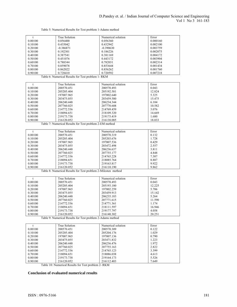
Table 5: Numerical Results for Test problem 1-Adams method
t 0.00100 0.10100 0.20100 0.30100 0.40100 0.50100 0.60100 0.70100 0.80100 0.90100
True Solution 0.056400 0.435042 -0.386871 0.192301 0.387541 0.451076 0.788344 0.859078 0.862022 0.728410
Numerical solution 0.056360 0.432942 -0.390630 0.186226 0.381169 0.443172 0.782031 0.853644 0.856262 0.720592
Error 0.000160 0.002100 0.003759 0.002075 0.004172 0.003904 0.002314 0.001434 0.001760 0.007218
Table 6: Numerical Results for Test problem 1- RKM
t 0.00100 0.10100 0.20100 0.30100 0.40100 0.50100 0.60100 0.70100 0.80100 0.90100
True Solution 200570.451 205205.404 197007.965 203475.055 206240.448 207760.025 214772.536 218094.651 219173.738 216120.052
Numerical solution 200570.493 205192.581 197002.640 203459.580 206234.344 207770.608 214769.459 218109.320 219175.419 216138.085
Error 0.043 12.824 5.325 15.475 6.104 10.582 3.076 14.669 1.680 18.033
Table 7: Numerical Results for Test problem 2-EM method
t 0.00100 0.10100 0.20100 0.30100 0.40100 0.50100 0.60100 0.70100 0.80100 0.90100
True Solution 200570.451 205205.404 197007.965 203475.055 206240.448 207760.025 214772.536 218094.651 219173.738 216120.052
Numerical solution 200570.319 205203.676 197007.536 203472.498 206236.637 207755.177 214765.228 218085.764 219163.817 216110.190
Error 0.132 1.728 0.429 2.557 3.811 4.848 7.307 8.887 9.922 9.862
Table 8: Numerical Results for Test problem 2-Milesten method
t 0.00100 0.10100 0.20100 0.30100 0.40100 0.50100 0.60100 0.70100 0.80100 0.90100
True Solution 200570.451 205205.404 197007.965 203475.055 206240.448 207760.025 214772.536 218094.651 219173.738 216120.052
Numerical solution 200570.493 205193.180 197002.259 203459.913 206235.183 207771.615 214771.361 218111.597 219177.797 216140.302
Error 0.043 12.225 5.706 15.142 5.264 11.590 1.174 16.946 4.058 20.251
Table 9: Numerical Results for Test problem 2-Adams method
t 0.00100 0.10100 0.20100 0.30100 0.40100 0.50100 0.60100 0.70100 0.80100 0.90100
True Solution 200570.451 205205.404 197007.965 203475.055 206240.448 207760.025 214772.536 218094.651 219173.738 216120.052
Numerical solution 200570.309 205204.176 197007.136 203471.832 206236.476 207755.163 214765.123 218086.038 219164.173 216112.403
Error 0.122 1.029 0.790 1.223 1.972 2.822 3.399 4.613 5.526 7.649
Table 10: Numerical Results for Test problem 2- RKM
Conclusion of evaluated numerical results
ISSN : 0976-5166 181

D.Pandey et. al. / Indian Journal of Computer Science and Engineering Vol 1 No 3 161-183
From the results presented in tables 1-10, we may notice that the Milstein and RKM (Runge kutta Method)methods out perform the other two in accuracy. For RKM (Runge kutta Method) method the errors decrease as N increases for all N values and all 2tests problems (with the exception of N=10000 and test problem 1). The same is more or less true for Milstein’s method. For the other two methods (EM and Adams) the error increase for N = 20000 for test problem 1-3. Looking at tables 1-10where absolute values of the errors at different t values are given we notice the following.For Test 1, Milstein and Adams2 methods are the best and of comparable accuracy.For Test problem 2, all 4 methods are of similar accuracy. We may notice though that the EM and Adams method have oscillating errors.
In most cases, the Adams method and EM does not provide a better performance than the RKM (Runge kutta Method) method, in other words, for SDE with multiplicative noise, the Adams method is the same as the FDM method. Meanwhile the construction of code is much more complicated than the RKM (Runge kutta Method). The results confirms that when the stochastic error becomes more dominant, the adams method loses its power (compare also(Denk and schaffler [7])).According to (Denk and schaffler [7]). The main reason for the low accuracy of Adams method in the multiplicative case is that the high order of the deterministic convergence is surpassed by the low order of stochastic convergence. The RKM (Runge kutta Method)can overcome this problem well. The higher order term employed in stochastic part can benefit the order of convergence. The numerical results can confirm that the performance of RKM (Runge kutta Method) is much better than the original one.Overall, it appears that the RKM (Runge kutta Method) performed consistently better than all other methods with respect to accuracy with Milstein method second best.
References:
[1] Boyce, W,E. and DiPrima, R.C. (1997), Elementary Differential Equations and Boundary Value Problems, Wiley. [2] Burrage, K. and Burrage, P.M. (1996), High Strong Order Explicit Runge-Kutta Methods for Stochastic Ordinary Differential Equations; Applied Numerical Mathematics, 22, 81-101. [3] Clark, C.W. (1990), Mathematical Bio-economics, Wiley. [4] Clark, C.W. (1979), Mathematical Models in the Economics of Renewable Resources, SIAM Review, 21, 81-99. [5] Cyganowski, S. (1996), A Maple Package for Stochastic Differential Equations, p. 223-223, in: Computational Techniques and Applications: CTA95, R.L. May, A.K. Easton (Eds), World Scientific. [6] Cyganowski, S., Kloeden, P.E., and Ombach J. (2001), From Elementary Probability to stochastic Differential Equations with Maple, Springer Verlag. [7] Denk, G., and Schaffler, S. (1997), Adams Methods for the Efficient Solution of Stochastic Differential Equations with Additive Noise, Computing, 59, 153-161. [8]Dwyer, G. P., Jr. and Williams, K.B., (2003), Portable Random Number Generators, J. of Economics Dynamics and Control, 27, 645-650. [9] Fisz, M. (1963), Probability Theory and Mathematical Statistics, John Wiley & Sons, Inc. [10] Gard, T.C. (1988), Introduction to Stochastic Differential Equations, Marcel Dekker Inc. [11] Gray, R.M. (1988), Probability, Random Processes and Ergodic Properties, Springer-Verlag. [12] Grewal .B.S. Numerical Methods in Engineering and Sciences with Programmes in FOTRAN 77, C and C++ (2009) Khanna Publishers. [13] Heath, M.T. (2001), Scientific Computing-An Introductory Survey, McGraw Hill. [14] Higham, D.J. (2001), An Algorithmic Introduction to Numerical Simulation of Stochastic Differential Equations, SIAM Review, 43, No.3, 525-546. [15] Higham, D.J. and Kloeden, P.E. (2001), Maple and Matlab for Stochastic Differential Equations in Finance, Mathematics Research Report No.3, Univ. of Strathclyde. [16] Hofmann, N. (1995), Stability of Weak Numerical Schemes for Stochastic Differential Equations, Mathematics and Computers in Simulation, 38, 63-68. [17] Kloeden, P.E. and Platen, E. (1989), Review: A Survey of Numerical Methods for Stochastic Differential Equations, Stochastic Hydrol. Hydraul., 3, 155-178. [18] Kloeden, P.E. Platen, E., and Schurz, H. (197), Numerical Solution of Stochastic Differential Equations Through Computer Experiments, Springer-Verlag. [19] Kloeden, P.E. and Platen, E. (1999), Numerical Solution of Stochastic Differential Equations, Springer-Verlag. [20] Lambert, J.D. (1973), Computational Methods in Ordinary Differential Equations, John Wiley & Sons. [21] Liske, H. and Platen, E. (1987), Simulation Studies On Time Discrete Diffusion Approximations, Mathematics and Computers in Simulation, 29, 253-260. [22] McDonald, A.D., Sandal, L.K., and Steinshamn, S.I. (2002), Implications of A Nested Stochastic/Deterministic Bio-economic Model for A Pelagic Fishery, Ecological Modeling, 149, 193-201. [23] Mikosch, T. (2001), Elementary Stochastic Calculus with Finance in View, World Scientific. [24] Milstein, G.N (1974), Approximate Integration of Stochastic Differential Equations, Theory Probab. Appl., 19, 557-562. [25] Oksendal, B. (1998), Stochastic Differential Equations: An Introduction with Application, Springer-Verlag.
ISSN : 0976-5166 182

D.Pandey et. al. / Indian Journal of Computer Science and Engineering Vol 1 No 3 161-183
[26] Platen, E. (1995), On Weak Implicit and Predictor-corrector Methods, Mathematics and Computers in Simulation, 38, 69-76. [27] Satio, Y., and Mitsui, T. (1996), Stability Analysis of Numerical Schemes for Stochastic Differential Equations, SIAM J. Numer. Anal., 3, No.6, 2254-2267. [28] S. Butterworth., Susan J. Johnston, Anbabela.,Aabranda ,(2010) Pretesting the Likely Efficacy of Suggested Management Approaches to Data-Poor Fisheries., Marine and Coastal Fisheries: Dynamics, Management, and Ecosystem Science 2:131–145 [29] Smith .G.D., Numerical solution of Partial differential equations: Finte Diffrence Methods., (1986) [30] Timothy Sauer (2008), Numerical Solution of Stochastic Differential Equations in Finance Conference proceding., Int conference in Management. : 21-41 [31] William H.Press., Saul A.Tukolsky., William T.vetterling., B.P.Flannery., (2005) Numerical Recipes in FORTRAN The art of Scientific Computing Second Edition. Cambridge University Press.
ISSN : 0976-5166 183