ScoutAutomatedPrintCode - pearsoncmg.com

http://www.facebook.com/share.php?u=http://www.informIT.com/title/9780136627159

http://twitter.com/?status=RT: download a free sample chapter http://www.informit.com/title/9780136627159

https://plusone.google.com/share?url=http://www.informit.com/title/9780136627159

http://www.linkedin.com/shareArticle?mini=true&url=http://www.informit.com/title/9780136627159

http://www.stumbleupon.com/submit?url=http://www.informit.com/title/9780136627159/Free-Sample-Chapter

Microsoft Office Specialist

MOS Study Guide for Microsoft Excel Exam MO-200

Joan Lambert

Exam MO-200

Editor-in-ChiefBrett Bartow

Executive EditorLoretta Yates

Development EditorSonglin Qiu

Sponsoring EditorCharvi Arora

Managing EditorSandra Schroeder

Senior Project EditorTracey Croom

Copy EditorDan Foster

IndexerCheryl Ann Lenser

ProofreaderAbigail Manheim

Technical EditorBoyd Nolan

Editorial AssistantCindy Teeters

Cover DesignerTwist Creative, Seattle

CompositorcodeMantra

MOS Study Guide for Microsoft Excel Exam MO-200

Published with the authorization of Microsoft Corporation by: Pearson Education, Inc.

Copyright © 2020 by Pearson Education, Inc.

All rights reserved. This publication is protected by copyright, and permission must be obtained from the publisher prior to any prohibited reproduction, storage in a retrieval system, or transmission in any form or by any means, electronic, mechanical, photocopying, recording, or likewise. For information regarding permissions, request forms, and the appropriate contacts within the Pearson Education Global Rights & Permissions Department, please visit www.pearson.com/permissions

No patent liability is assumed with respect to the use of the information contained herein. Although every precaution has been taken in the preparation of this book, the publisher and author assume no responsibility for errors or omissions. Nor is any liability assumed for damages resulting from the use of the information contained herein.

ISBN-13: 978-0-13-662715-9ISBN-10: 0-13-662715-3

Library of Congress Control Number: 2020931638

ScoutAutomatedPrintCode

TrademarksMicrosoft and the trademarks listed at https://www.microsoft.com on the “Trademarks” webpage are trademarks of the Microsoft group of companies. All other marks are property of their respective owners.

Warning and DisclaimerEvery effort has been made to make this book as complete and as accurate as possible, but no warranty or fitness is implied. The information provided is on an “as is” basis. The author, the publisher, and Microsoft Corporation shall have neither liability nor responsibility to any person or entity with respect to any loss or damages arising from the information contained in this book or from the use of the programs accompanying it.

Special SalesFor information about buying this title in bulk quantities, or for special sales opportunities (which may include electronic versions; custom cover designs; and content particular to your business, training goals, marketing focus, or branding interests), please contact our corporate sales department at [email protected] or (800) 382-3419.

For government sales inquiries, please contact [email protected].

For questions about sales outside the U.S., please contact [email protected].

http://www.pearson.com/permissions

https://www.microsoft.com

mailto:[email protected]



iii

ContentsIntroduction vi

1 Manage worksheets and workbooks 1

Objective 1.1: Import data into workbooks . . . . . . . . . . . . . . . . . . . . . . . . . . . . . . 2

Import data from delimited text files 2

Objective 1.2: Navigate within workbooks . . . . . . . . . . . . . . . . . . . . . . . . . . . . . . 9

Search for data within a workbook 9Navigate to named cells, ranges, or workbook elements 10Insert and remove hyperlinks 11

Objective 1.3: Format worksheets and workbooks . . . . . . . . . . . . . . . . . . . . . . .18

Modify page setup 18Adjust row height and column width 19Customize headers and footers 21

Objective 1.4: Customize options and views . . . . . . . . . . . . . . . . . . . . . . . . . . . 26

Customize the Quick Access Toolbar 26Modify the display of content 29Display multiple parts of a worksheet 32Display formulas 33Modify basic workbook properties 33

Objective 1.5: Configure content for collaboration . . . . . . . . . . . . . . . . . . . . . 36

Inspect workbooks for issues 36Print workbook content 42Save workbooks in alternative file formats 47

iv

Contents

2 Manage data cells and ranges 53

Objective 2.1: Manipulate data in worksheets . . . . . . . . . . . . . . . . . . . . . . . . . . 54

Create data 54Reuse data 57Modify worksheet structure 62

Objective 2.2: Format cells and ranges . . . . . . . . . . . . . . . . . . . . . . . . . . . . . . . . 65

Merge and unmerge cells 65Modify cell alignment, orientation, and indentation 66Wrap text within cells 68Apply cell formats and styles 69Apply number formats 70Reapply existing formatting 73

Objective 2.3: Define and reference named ranges . . . . . . . . . . . . . . . . . . . . . 76

Objective 2.4: Summarize data visually . . . . . . . . . . . . . . . . . . . . . . . . . . . . . . . . 80

Format cells based on their content 80Insert sparklines 83

3 Manage tables and table data 87

Objective 3.1: Create and format tables . . . . . . . . . . . . . . . . . . . . . . . . . . . . . . . 88

Create an Excel table from a cell range 88Apply styles to tables 91Convert a table to a cell range 92

Objective 3.2: Modify tables . . . . . . . . . . . . . . . . . . . . . . . . . . . . . . . . . . . . . . . . . . 95

Add or remove table rows and columns 95Configure table style options 97

Objective 3.3: Filter and sort table data . . . . . . . . . . . . . . . . . . . . . . . . . . . . . . .101

Filter tables 101Sort tables 103

v

Contents

4 Perform operations by using formulas and functions 107

Objective 4.1: Insert references in formulas . . . . . . . . . . . . . . . . . . . . . . . . . . . 108

Insert relative, absolute, and mixed references 108Reference named cell ranges and tables in formulas 110

Objective 4.2: Calculate and transform data by using functions . . . . . . . . .112

Perform calculations by using the SUM(), AVERAGE(), MAX(), and MIN() functions 112Count cells by using the COUNT(), COUNTA(), and COUNTBLANK() functions 116Perform conditional operations by using the IF() function 118

Objective 4.3: Format and modify text by using functions . . . . . . . . . . . . . .121

Select text by using the LEFT(), MID(), and RIGHT() functions 121Format text by using the UPPER(), LOWER(), and PROPER() functions 123Count characters by using the LEN() and LENB() functions 125Combine text by using the CONCAT() and TEXTJOIN() functions 125

5 Manage charts 129

Objective 5.1: Create charts . . . . . . . . . . . . . . . . . . . . . . . . . . . . . . . . . . . . . . . . . . 130

Objective 5.2: Modify charts . . . . . . . . . . . . . . . . . . . . . . . . . . . . . . . . . . . . . . . . . 137

Modify chart content 137Modify chart elements 140

Objective 5.3: Format charts . . . . . . . . . . . . . . . . . . . . . . . . . . . . . . . . . . . . . . . . . 143

Apply layouts and styles 143Provide alternative text for accessibility 144

Index 147

vi

IntroductionThe Microsoft Office Specialist (MOS) certification program has been designed to validate your knowledge of and ability to use programs in the Microsoft Office suite of programs. This book has been designed to guide you in studying the types of tasks you are likely to be required to demonstrate in Exam MO-200: Microsoft Excel 2019.

See Also For information about the tasks you are likely to be required to demonstrate in Exam MO-201: Microsoft Excel 2019 Expert, see MOS 2019 Study Guide for Microsoft Excel Expert by Paul McFedries (Microsoft Press, 2020).

Who this book is forMOS 2019 Study Guide for Microsoft Excel is designed for experienced computer users seeking Microsoft Office Specialist certification in Excel 2019 or the equivalent version of Excel for Office 365.

MOS exams for individual programs are practical rather than theoretical. You must demonstrate that you can complete certain tasks or projects rather than simply answer questions about program features. The successful MOS certification candidate will have at least six months of experience using all aspects of the application on a regular basis—for example, using Excel at work or school to create and manage work-books and worksheets, modify and format cell content, summarize and organize data, present data in tables and charts, perform data operations by using functions and for-mulas, and insert and format objects on worksheets.

As a certification candidate, you probably have a lot of experience with the program for which you want to become certified. Many of the procedures described in this book will be familiar to you; others might not be. Read through each study section and ensure that you are familiar with the procedures, concepts, and tools discussed. In some cases, images depict the tools you will use to perform procedures related to the skill set. Study the images and ensure that you are familiar with the options available for each tool.

vii

Introduction

How this book is organizedThe exam coverage is divided into chapters representing broad skill sets that correlate to the functional groups covered by the exam. Each chapter is divided into sections addressing groups of related skills that correlate to the exam objectives. Each section includes review information, generic procedures, and practice tasks you can complete on your own while studying. We provide practice files you can use to work through the practice tasks, and results files you can use to check your work. You can practice the generic procedures in this book by using the practice files supplied or by using your own files.

Throughout this book, you will find Exam Strategy tips that present information about the scope of study that is necessary to ensure that you achieve mastery of a skill set and are successful in your certification effort.

IMPORTANT The Excel 2019 program is not available from this website. You should purchase and install that program before using this book.

You will save the completed versions of practice files that you modify while working through the practice tasks in this book. If you later want to repeat the practice tasks, you can download the original practice files again.

viii

Introduction

The following table lists the practice files provided for this book.

Folder and objective group Practice files Result files

MOSExcel2019\Objective1Manage worksheets and workbooks

Excel_1-1.xlsx Excel_1-2.xlsxExcel_1-3.xlsxExcel_1-4.xlsxExcel_1-5.xlsx

Excel_1-1_Results subfolder: ■ Excel_1-1_results.xlsx ■ MyBlank_results.xlsx ■ MyCalc_results.xlsx

Excel_1-2_results.xlsxExcel_1-3_results.xlsxExcel_1-4_results.xlsxExcel_1-5_Results subfolder:

■ Excel_1-5a_results.xlsx ■ MOS-Compatible.xls ■ MOS-Template.xltm

MOSExcel2019\Objective2Manage data cells and ranges

Excel_2-1.xlsx Excel_2-2.xlsxExcel_2-3.xlsx

Excel_2-1_results.xlsxExcel_2-2_results.xlsxExcel_2-3_results.xlsx

MOSExcel2019\Objective3Manage tables and table data

Excel_3-1.xlsxExcel_3-2.xlsxExcel_3-3.xlsx


MOSExcel2019\Objective4Perform operations by using formulas and functions

Excel_4-1a.xlsxExcel_4-1b.xlsxExcel_4-1c.xlsxExcel_4-2.xlsxExcel_4-3.xlsx

Excel_4-1a_results.xlsxExcel_4-1b_results.xlsxExcel_4-1c_results.xlsxExcel_4-2_results.xlsxExcel_4-3_results.xlsx

MOSExcel2019\Objective5Manage charts

Excel_5-1.xlsxExcel_5-2.xlsxExcel_5-3a.xlsxExcel_5-3b.jpgExcel_5-3c.txt


ix

Introduction

Adapt procedure stepsThis book contains many images of user interface elements that you’ll work with while performing tasks in Excel on a Windows computer. Depending on your screen resolution or app window width, the Excel ribbon on your screen might look different from that shown in this book. (If you turn on Touch mode, the ribbon displays signifi-cantly fewer commands than in Mouse mode.) As a result, procedural instructions that involve the ribbon might require a little adaptation.

Simple procedural instructions use this format:

■ On the Insert tab, in the Illustrations group, click the Chart button.

If the command is in a list, our instructions use this format:

■ On the Home tab, in the Editing group, click the Find arrow and then, in the Find list, click Go To.

If differences between your display settings and ours cause a button to appear differ-ently on your screen than it does in this book, you can easily adapt the steps to locate the command. First click the specified tab, and then locate the specified group. If a group has been collapsed into a group list or under a group button, click the list or button to display the group’s commands. If you can’t immediately identify the button you want, point to likely candidates to display their names in ScreenTips.

The instructions in this book assume that you’re interacting with on-screen elements on your computer by clicking (with a mouse, touchpad, or other hardware device). If you’re using a different method—for example, if your computer has a touchscreen interface and you’re tapping the screen (with your finger or a stylus)—substitute the applicable tapping action when you interact with a user interface element.

Instructions in this book refer to user interface elements that you click or tap on the screen as buttons, and to physical buttons that you press on a keyboard as keys, to conform to the standard terminology used in documentation for these products.

x

Introduction

Ebook editionIf you’re reading the ebook edition of this book, you can do the following:

■ Search the full text

■ Print

■ Copy and paste

You can purchase and download the ebook edition from the Microsoft Press Store at:

MicrosoftPressStore.com/MOSExcel200/detail

Stay in touchLet’s keep the conversation going! We’re on Twitter at:

https://twitter.com/MicrosoftPress

http://MicrosoftPressStore.com/MOSExcel200/detail

https://twitter.com/MicrosoftPress

xi

About the authorJOAN LAMBERT has worked closely with Microsoft technologies since 1986, and in the training and certification industry since 1997, guiding the translation of technical information and requirements into useful, relevant, and measurable resources for people who are seeking certification of their computer skills or who simply want to get things done efficiently.

Joan is the author or coauthor of more than four dozen books about Windows and Office (for Windows, Mac, and iPad), six generations of Microsoft Office Specialist certification study

guides, video-based training courses for SharePoint and OneNote, QuickStudy guides for Windows 10 and Office 2016, and GO! series books for Outlook.

Joan is a Microsoft Certified Professional, Microsoft Office Specialist Master (for all versions of Office since Office 2003), Microsoft Certified Technology Specialist (for Windows and Windows Server), Microsoft Certified Technology Associate (for Windows), Microsoft Dynamics Specialist, and Microsoft Certified Trainer. She is also certified in Adobe InDesign and Intuit QuickBooks.

A native of the Pacific Northwest and enthusiastic world traveler, Joan is now blissfully based in America’s Finest City with her simply divine daughter Trinity, Thai host daughter Thopad, and their faithful canine, feline, and aquatic companions.

This page intentionally left blank

53

Objective group 2

The skills tested in this section of the Microsoft Office Specialist exam for Microsoft Excel 2019 relate to managing cells and cell content in worksheets. Specifically, the following objectives are associated with this set of skills:

2.1 Manipulate data in worksheets2.2 Format cells and ranges2.3 Define and reference named ranges2.4 Summarize data visually

Excel stores data in individual cells of the worksheets within a workbook. You can process or reference the data in each cell in many ways, either individually or in logical groups. A set of contiguous data cells is a data range. A data range can be as small as a short list of dates or as large as a multicolumn table that includes thousands of rows of data.

You might populate a worksheet from scratch or by creating, reusing, or cal-culating data from other sources. You can perform various operations on data when pasting it into a worksheet, either to maintain the original state of the data or to change it. When creating data from scratch, you can quickly enter large amounts of data that follows a pattern by filling a numeric or alphanu-meric data series. You can fill any of the default series that come with Excel or create a custom data series.

This chapter guides you in studying ways of working with the content and appearance of cells and the organization of data.

Manage data cells and ranges

2

54

Objective group 2 Manage data cells and ranges

IMPORTANT If you apply an Excel table format to a data range, it then becomes a table, which has additional functionality beyond that of a data range. Tables are discussed in Objective group 3, “Manage tables and table data.” The functionality in this chapter pertains explicitly to data ranges that are not formatted as Excel tables.

Objective 2.1: Manipulate data in worksheetsThe most basic method of inserting data in cells is by entering it manually, which is a prerequisite skill for this exam. This section discusses methods of creating and reusing data to fill a worksheet.

Create dataWhen you create the structure of a data range, or a series of formulas, you can auto-mate the process of completing data patterns (such as January, February, March) or copying calculations from one row or column to those adjacent. Automation saves time and can help prevent human errors.

You can quickly fill adjacent cells with data that continues a formula or a series of numbers, days, or dates, either manually from the Fill menu, or automatically by dragging the fill handle. When copying or filling data by using the Fill menu com-mands, you can set specific options in the Series dialog box for the pattern of the data sequence you want to create.

The Fill menu and Series dialog box

55

Objective 2.1: Manipulate data in worksheets

You can use the fill functionality to copy text data, numeric data, or cell formatting (such as text color, background color, and alignment) to adjacent cells.

When creating a series based on one or more selected cells (called filling a series), you can select from the following series types:

■ Linear Excel calculates the series values by adding the value you enter in the Step Value box to each cell in the series.

■ Growth Excel calculates the series values by multiplying each cell in the series by the step value.

■ Date Excel calculates the series values by incrementing each cell in the series of dates, designated by the Date Unit you select, by the step value.

■ Auto Fill This option creates a series that produces the same results as drag-ging the fill handle.

When you use the Auto Fill feature, either from the Fill menu or by dragging the fill handle, the Auto Fill Options button appears in the lower-right corner of the fill range. Clicking the button displays a menu of fill options. The fill options vary based on the type of content being filled.

Fill handle

Auto Fill Options button

Auto Fill Options menu

The Auto Fill Options menu when filling a date series

Tip The Auto Fill Options button does not appear when you copy data to adjacent cells.

You can use the Auto Fill feature to create sequences of numbers, days, and dates; to apply formatting from one cell to adjacent cells; or, if you use Excel for more sophis-ticated purposes, to create sequences of data generated by formulas, or custom sequences based on information you specify. You can also use the fill functionality to copy text or numeric data within the column or row.

2

56


To fill a simple numeric, day, or date series

1. Do either of the following:

● In the upper-left cell of the range you want to fill, enter the first number, day, or date of the series you want to create.

● To create a series in which numbers or dates increment by more than one, enter the first two or more values of the series in the first cells of the range you want to fill.

Tip Enter as many numbers or dates as are necessary to establish the series.

2. If creating a numeric series that has a specific number format (such as currency, percentage, or fraction), apply the number format you want from the Number group on the Home tab.

3. Select the cell or cells that define the series.


● Drag the fill handle down or to the right to create an increasing series.

● Drag the fill handle up or to the left to create a decreasing series.

Tip When using the fill handle, you can drag in only one direction at a time; to fill a range of multiple columns and rows, first drag in one direction, then release the mouse button and drag the new fill handle in the other direction. The default fill series value is indicated in a tooltip as you drag.

5. If the series doesn’t automatically fill correctly, click the Auto Fill Options button and then, on the Auto Fill Options menu, click Fill Series.

To fill a specific day or date series

1. Fill the series. Immediately after you release the mouse button, click the Auto Fill Options button that appears in the lower-right corner of the cell range.

2. On the Auto Fill Options menu, click Fill Days, Fill Weekdays, Fill Months, or Fill Years.

57


To set advanced options for a numeric, day, or date series

1. Enter the number or date beginning the series, and then select the cell range you want to fill.

2. On the Home tab, in the Editing group, in the Fill list, click Series.

3. In the Series dialog box, select the options you want, and then click OK.

To exclude formatting when filling or copying data

1. Drag the fill handle to fill the series or copy the data, and then click the Auto Fill Options button.

2. On the Auto Fill Options menu, click Fill Without Formatting.

Reuse dataIf the content you want to work with in Excel already exists elsewhere—such as in another worksheet or workbook or in a document—you can cut or copy the data from the source location to the Microsoft Office Clipboard and then paste it into the work-sheet. If the content exists but not in the format that you need it, you might be able to reform the content to fit your needs by using the CONCATENATE function or the Flash Fill feature.

Paste data by using special paste optionsYou can insert cut or copied cell contents into empty cells or directly into an existing table or data range. Cutting, copying, and pasting content (including columns and rows) in a worksheet are basic tasks that, as a certification candidate, you should have extensive experience with. If you need a refresher on these subjects, see the “Pre-requisites” section of the Exam Overview. This section contains information about Excel-specific pasting operations that you may be required to demonstrate to pass Exam MO-200 and become certified as a Microsoft Office Specialist for Excel 2019.

When pasting data, you have several options for inserting values, formulas, format-ting, or links to the original source data into the new location. Paste options are avail-able from the Paste menu, from the shortcut menu, and from the Paste Options menu that becomes temporarily available when you paste content.

Excel also offers some advanced pasting techniques you can use to modify data while pasting it into a worksheet. Using the Paste Special feature, you can perform mathematical operations when you paste data over existing data, you can transpose

2

58


columns to rows and rows to columns, and you can be selective about what you want to paste from the source cells.

The available paste options vary based on the type and formatting of the content you’re pasting

Paste specific aspects of copied content, or modify content while pasting it

You have the option to paste only values without formatting, formatting without values, formulas, comments, and other specific aspects of copied content. You can also link to data rather than inserting it, so that if the source data changes, the copied data will also change.

59


Paste options that are commonly used in business, and that you should be comfort-able with when taking Exam MO-200, include the following:

■ Pasting values When you reuse a value that is the result of a formula, it is often necessary to paste only the value—the result of the formula—rather than the actual cell content.

■ Pasting formats This is somewhat like using the Format Painter and can be useful when you want to build a structure on a worksheet that already exists elsewhere.

■ Transposing cells Transposing content switches it from columns to rows or from rows to columns. This can be very useful when reusing content from one worksheet in another.

Original data Transposed data

Excel maintains cell formatting when transposing data

Exam Strategy Be familiar with all the Paste and Paste Special options.

2

60


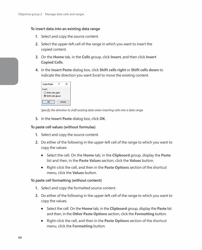
To insert data into an existing data range

1. Select and copy the source content.

2. Select the upper-left cell of the range in which you want to insert the copied content.

3. On the Home tab, in the Cells group, click Insert, and then click Insert Copied Cells.

4. In the Insert Paste dialog box, click Shift cells right or Shift cells down to indicate the direction you want Excel to move the existing content.

Specify the direction to shift existing data when inserting cells into a data range

5. In the Insert Paste dialog box, click OK.

To paste cell values (without formulas)


2. Do either of the following in the upper-left cell of the range to which you want to copy the values:

● Select the cell. On the Home tab, in the Clipboard group, display the Paste list and then, in the Paste Values section, click the Values button.

● Right-click the cell, and then in the Paste Options section of the shortcut menu, click the Values button.

To paste cell formatting (without content)

1. Select and copy the formatted source content.

2. Do either of the following in the upper-left cell of the range to which you want to copy the values:

● Select the cell. On the Home tab, in the Clipboard group, display the Paste list and then, in the Other Paste Options section, click the Formatting button.

● Right-click the cell, and then in the Paste Options section of the shortcut menu, click the Formatting button.

61


To transpose rows and columns


2. Do either of the following in the upper-left cell of the range to which you want to copy the transposed values:

● Select the cell. On the Home tab, in the Clipboard group, display the Paste list and then, in the Paste section, click the Transpose button.

● Right-click the cell, and then in the Paste Options section of the shortcut menu, click the Transpose button.

Tip Transposing data retains its formatting.

Fill data based on an adjacent columnThe Flash Fill feature looks for correlation between data that you enter in a column and the adjacent data. If it identifies a pattern of data entry based on the adjacent column, it fills the rest of the column to match the pattern. A common example of using Flash Fill is to divide full names in one column into separate columns of first and last names so you can reference them individually (for example, when creating form letters).

Flash Fill automatically fills cells with content from adjacent columns

2

62


To fill cells by using Flash Fill

1. In columns adjacent to the source content column, enter content in one or more cells to establish the pattern of content reuse.

2. Select the next cell below the cells that establish the pattern. (Do not select a range of cells.)


● On the Home tab, in the Editing group, click Fill, and then click Flash Fill. ● Press Ctrl+E.

Tip If the Flash Fill operation doesn’t work as intended, click the Flash Fill Options button that appears in the lower-right corner of the first filled cell and then, on the menu, click Undo Flash Fill. Enter content in additional cells to further establish the pattern, and then try again.

Modify worksheet structureInsert and delete multiple columns or rowsTo insert rows or columns

1. Select the number of rows you want to insert, starting with the row above which you want the inserted rows to appear, or select the number of columns you want to insert, starting with the column to the left of which you want the inserted columns to appear.


● On the Home tab, in the Cells group, click the Insert button.

● Right-click the selection, and then click Insert.

To delete selected rows or columns

➜ On the Home tab, in the Cells group, click the Delete button.

➜ Right-click the selection, and then click Delete.

63


Insert and delete cellsTo insert cells in an existing data range

1. Select the number of cells you want to insert, in the location in which you want to insert them.

2. On the Home tab, in the Cells group, click Insert and then Insert Cells.

3. In the Insert dialog box, select Shift cells right or Shift cells down to indicate the direction in which you want to move the existing data to make room for the new cells. Then click OK. 2


64

Objective 2.1 practice tasksThe practice file for these tasks is in the MOSExcel2019\Objective2 practice file folder. The folder also contains a result file that you can use to check your work.

➤ Open the Excel_2-1 workbook, and complete the following tasks by using the data in cells B4:G9 of the Ad Buy Constraints worksheet:

❑ Paste only the values and formatting into the range beginning at B18.

❑ Paste only the formulas into the range beginning at B25.

❑ Paste only the formatting (but not the content) into the range beginning at B32.

❑ Delete rows to move the headings to row 1.

❑ Delete columns to move the Magazine column to column A.

❑ Cut the data from the Mag3 row (B4:F4) and insert it into the Mag2 row (B3:F3).

❑ Move the Cost Per Ad data to the left of the Total Cost cells.

❑ Insert two blank cells in positions B8:B9, shifting any existing data down.

❑ Transpose the names in the Magazine column (cells A1:A6) to the first row of a new worksheet.

➤ On the Price List worksheet, do the following:

❑ Using the fill handle, fill cells A2:A21 with Item 1, Item 2, Item 3, and so on through Item 20.

❑ Fill cells B2:B21 with 10, 20, 30, and so on through 200.

❑ Fill cells C2:C21 with $3.00, $2.95, $2.90, and so on through $2.05.

❑ Copy the background and font formatting from cell A1 to cells A2:A21. Then delete the content of cell A1 (but not the cell).

➤ Save the Excel_2-1 workbook and open the Excel_2-1_results workbook. Compare the two workbooks to check your work. Then close the open workbooks.

65

Objective 2.2: Format cells and ranges


Merge and unmerge cellsWorksheets that involve data at multiple hierarchical levels often use horizontal and vertical merged cells to clearly delineate relationships. Excel provides the following three merge options:

■ Merge & Center This option merges the cells across the selected rows and columns and centers the data from the first selected cell in the merged cell.

■ Merge Across This option creates a separate merged cell for each row in the selection area and maintains default alignment for the data type of the first cell of each row of the merged cells.

■ Merge Cells This option merges the cells across the selected rows and columns and maintains default alignment for the data type of the first cell of the merged cells.

In the case of Merge & Center and Merge Cells, data in selected cells other than the first is deleted. In the case of Merge Across, data in selected cells other than the first cell of each row is deleted.

Merged columns Merged rows

Merging columns or rows retains the content of the first cell

To merge selected cells

➜ On the Home tab, in the Alignment group, click the Merge & Center button to center and bottom-align the entry from the first cell.

➜ On the Home tab, in the Alignment group, display the Merge & Center list, and then click Merge Across to create a separate merged cell on each selected row, maintaining the horizontal alignment of the data type in the first cell of each row.

➜ On the Home tab, in the Alignment group, display the Merge & Center list, and then click Merge Cells to merge the entire selection, maintaining the horizontal alignment of the data type in the first cell.

2

66


To unmerge selected cells

➜ On the Home tab, in the Alignment group, click the Merge & Center button to deselect it.

Modify cell alignment, orientation, and indentationStructural formatting can be applied to a cell, a row, a column, or the entire worksheet. However, some kinds of formatting can detract from the readability of a worksheet if they are applied haphazardly.

Two-letter indent Wrapped text Rotated text

Structural cell formatting

Tip By default, row height is dynamic and increases to fit the text in its cells. If you manually change the height of a row and then change the size or amount of content in that row, you might have to set or reset the row height. For information about adjusting row height, see “Objective 1.3: Format worksheets and workbooks.”

The formatting you might typically apply to a row or column includes the following:

■ Alignment You can specify a horizontal alignment (Left, Center, Right, Fill, Justify, Center Across Selection, and Distributed) and vertical alignment (Top, Center, Bottom, Justify, or Distributed) of a cell’s contents. The defaults are Left and Top, but in many cases another alignment will be more appropriate.

■ Orientation By default, entries are horizontal and read from left to right. You can rotate entries for special effect or to allow you to display more information on the screen or a printed page. This capability is particularly useful when you have long column headings above columns of short entries.

67


■ Indentation You can specify an indent distance from the left or right side when you choose those horizontal alignments, or from both sides when you choose a distributed horizontal alignment. A common reason for indenting cells is to create a list of subitems without using a second column.

Tip You can change the text alignment, text control, text direction, and text orientation set-tings on the Alignment tab of the Format Cells dialog box. There are many ways to open the Format Cells dialog box to a specific tab. You may use any method you want.

To open the Format Cells dialog box to the most recently used tab

➜ On the Home tab, click the Font dialog box launcher.

➜ Press Ctrl+1.

To align entries within selected cells

➜ On the Home tab, in the Alignment group, click the Align Left, Center, or Align Right button to specify horizontal alignment, or click the Top Align, Middle Align, or Bottom Align button to specify vertical alignment.

➜ On the Home tab, click the Alignment dialog box launcher. On the Alignment tab of the Format Cells dialog box, in the Horizontal and Vertical lists, click the cell alignment you want.

Configure text alignment, indents, orientation, and wrapping options at one time from the Format Cells dialog box

2

68


Exam Strategy Many more text alignment options are available from the Format Cells dialog box than from the Format group of the Home tab. Ensure that you are familiar with these options.

To change the orientation of the text in selected cells

1. On the Home tab, in the Alignment group, click the Orientation button to display the Alignment tab of the Format Cells dialog box.

2. In the Orientation area, do either of the following:

● Drag the red diamond to the angle you want.

● In the Degrees list, click the angle you want.

The Text preview changes to display the effect of your selection.

3. In the Format Cells dialog box, click OK.

To indent the content of selected cells

1. On the Home tab, click the Alignment dialog box launcher.

2. On the Alignment tab of the Format Cells dialog box, in the Text alignment section, do the following:

a. In the Horizontal list, select Left (Indent), Right (Indent), or Distributed (Indent).

b. In the Indent box, enter or select the number of characters by which you want to indent the text. Then click OK.

3. In the Format Cells dialog box, click OK.

Wrap text within cellsBy default, Excel does not wrap text in a cell. Instead, it allows the entry to overflow into the surrounding cells (to the right from a left-aligned cell, to the left from a right-aligned cell, and to both sides from a center-aligned cell) if those cells are empty, or it hides the part that won’t fit if the surrounding cells contain content. To make the entire entry visible, you can allow the cell entry to wrap to multiple lines.

Tip Wrapping text increases the height of the cell. Increasing the height of one cell increases the height of the entire row.

69


To wrap long entries in selected cells

➜ On the Home tab, in the Alignment group, click the Wrap Text button.

Apply cell formats and stylesBy default, the font used for text in a new Excel worksheet is 11-point Calibri, but you can use the same techniques you would use in any Office 2019 program to change the font and the following font attributes:

■ Size

■ Style

■ Color

■ Underline

As a certification candidate, you should be very familiar with methods of applying character formatting from the Font group on the Home tab, from the Mini Toolbar, and from the Font, Border, and Fill tabs of the Format Cells dialog box.

Cell Styles are preconfigured sets of cell formats, some tied to the workbook theme colors and some with implied meanings. You can standardize formatting throughout workbooks by applying cell styles to content.

Some cell styles connote specific meanings

2

70


Exam Strategy Exam MO-200 requires that you demonstrate the ability to apply built-in cell styles. Creating custom cell styles is part of the objective domain for Exam MO-201, Microsoft Excel Expert.

To apply cell formatting from the Format Cells dialog box to selected cells

1. On the Home tab, click the Font dialog box launcher.

2. In the Format Cells dialog box, on the Font, Border, and Fill tabs, select the formatting you want to apply to the cell and its content. Then click OK.

To apply a cell style to a selected cell

1. On the Home tab, in the Styles group, click the Cell Styles button.

2. In the Cell Styles gallery, click the style you want.

Apply number formatsBy default, all the cells in a new worksheet are assigned the General number format. When setting up or populating a worksheet, you assign to cells the number format that is most appropriate for the type of information they contain. The format deter-mines not only how the information looks, but also how Excel can work with it.

Exam Strategy Knowing which number formats are appropriate for different types of data is important for efficient worksheet construction. Take the time to explore the formats so that you understand the available options.

You can assign a number format to a cell before or after you enter a number in it. You can also just start typing and have Excel intuit the format from what you type. (For example, if you enter 9/15, Excel makes the educated guess that you’re entering a date and applies the default date format d-mmm, resulting in 15-Sep.) When you allow Excel to assign a number format, or you choose a format from the Number Format list in the Number group on the Home tab, Excel uses the default settings for that format. You can change the currency symbol and the number of decimal places shown directly from the Number group. You can change many other settings (such as changing the format of calendar dates from 15-Sep to September 15, 2019) from the Format Cells dialog box.

71


Exam Strategy Exam MO-200 requires you to demonstrate that you can apply built-in number formats. Creating custom number formats is part of the objective domain for Exam MO-201, Microsoft Excel Expert.

Select a data format that will provide clear information to workbook readers

When you apply the Percentage number format to a cell, the cell displays the per-centage equivalent of the number. For example, the number 1 is shown as 100%, the number 5 as 500%, or the number 0.25 as 25%.

Tip On the Home tab, in the Number group, the button that applies the Percentage style has the ScreenTip Percent Style.

To apply a default number format to selected cells

➜ On the Home tab, in the Number group, display the Number Format list, and then click a format.

Tip If you want a number to be treated as text, apply the Text number format.

2

72


To display the percentage equivalent of a number

1. Select the cell or cells you want to format.


● On the Home tab, in the Number group, click the Percent Style button.

● Press Ctrl+Shift+%.

To display a number as currency


2. On the Home tab, in the Number group, do one of the following:

● To format the number in the default currency, click the Accounting Number Format button (labeled with the default currency symbol).

● To format the number in dollars, pounds, euros, yen, or Swiss francs, click the Accounting Number Format arrow, and then click the currency you want.

● To format the number in a currency other than those listed, click the Accounting Number Format arrow, and then click More Accounting Formats to display the Accounting options.

You can choose from hundreds of currencies

73


3. In the Format Cells dialog box, do the following, and then click OK:

a. In the Symbol list, select the currency symbol you want to display.

b. In the Decimal places box, enter or select the number of decimal places you want to display.

To display more or fewer decimal places for numbers


2. On the Home tab, in the Number group, do either of the following:

● To display more decimal places, click the Increase Decimal button.

● To display fewer (or no) decimal places, click the Decrease Decimal button.

To apply a number format with settings other than the default


2. On the Home tab, click the Number dialog box launcher.

3. On the Number tab of the Format Cells dialog box, select the type of number in the Category list.

4. Configure the settings that are specific to the number category, and then click OK.

Exam Strategy Exam MO-200 requires that you demonstrate the ability to apply built-in num-ber formats. Creating and managing custom number formats is part of the objective domain for Exam MO-201, Microsoft Excel Expert.

Reapply existing formattingIf you apply a series of formats to one or more cells—for example, if you format cell content as 14-point, bold, centered, red text—and then want to apply the same combination of formatting to other cells, you can copy the formatting. You can use the fill functionality to copy formatting to adjacent content, or use the Format Painter to copy formatting anywhere. When using the Format Painter, you first copy existing formatting from one or more cells, and then paste the formatting to other cells. You can use the Format Painter to paste copied formatting only once or to remain active until you turn it off.

2

74


To copy existing formatting to other cells

1. Select the cell that has the formatting you want to copy.

2. On the Mini Toolbar or in the Clipboard group on the Home tab, click the Format Painter button once if you want to apply the copied formatting only once, or twice if you want to apply the copied formatting multiple times.

3. With the paintbrush-shaped cursor, click or select the cell or cells to which you want to apply the copied formatting.

4. If you clicked the Format Painter button twice, click or select additional cells you want to format. Then click the Format Painter button again, or press the Esc key, to turn off the Format Painter.

To fill formatting to adjacent cells

1. Select the cell that has the formatting you want to copy.

2. Drag the fill handle up, down, to the left, or to the right to encompass the cells you want to format.

3. On the Auto Fill Options menu, click Fill Formatting Only.


75


➤ Open the Excel_2-2 workbook, display the Employees worksheet, and do the following:

❑ Merge cells A13:C14 so that the hyperlink is centered in a double-height cell across the three columns.

➤ On the Expense Statement worksheet, do the following:

❑ Select the entire worksheet and turn on text wrapping.

❑ Turn off text wrapping in only rows 4, 5, and 9.

❑ Right-align the entries in column A.

❑ Bottom-align the headings in row 9.

❑ Apply the Angle Counterclockwise orientation to the headings in row 9.

❑ Format cell K10 to display its contents as currency with a US dollar symbol and no decimal places. Then apply the same formatting to cells K11:K23.

❑ Apply the 20% - Accent2 cell style to cells A9:K9.

➤ Save the Excel_2-2 workbook and open the Excel_2-2_results workbook. Compare the two workbooks to check your work. Then close the open workbooks.

76


Objective 2.3: Define and reference named rangesAs specified at the beginning of this chapter, a set of contiguous data cells is a data range. Data ranges are expressed in the format upper-left cell:lower-right cell—for example, A1:J10 defines the 100 cells within the area bound by cells A1 in the upper-left corner, J1 in the upper-right corner, J10 in the lower-right corner, and A10 in the lower-left corner. You can reference a data range (A1:J10) in a formula, or you can give the range a meaningful name (such as StudentGrades or PriceList) and then refer-ence the range name. Using named ranges can greatly simplify formulaic processes because you don’t have to find or remember the cell references, and if you add data to a named range, the new data is automatically included in any formulas that refer-ence the range.

Excel tables are assigned names automatically when you create them. Within each workbook, the first table you create is Table1, then Table2, and so on. You can refer-ence any table by its default name or change the numeric table names to something more meaningful so you can more easily reference them.

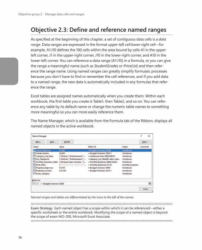
The Name Manager, which is available from the Formula tab of the Ribbon, displays all named objects in the active workbook.

Named ranges and tables are differentiated by the icons to the left of the names

Exam Strategy Each named object has a scope within which it can be referenced—either a specific worksheet or the entire workbook. Modifying the scope of a named object is beyond the scope of exam MO-200, Microsoft Excel Associate.

77

Objective 2.3: Define and reference named ranges

You can create and modify range names and table names (or the data defined by those names) from the Name Manager. However, if you’re simply naming a range or renaming a table, there’s an easier way:

■ You can name data ranges from the Name box at the left end of the Formula Bar.

■ You can rename tables from the Table Name box in the Properties group of the Design tool tab for tables.

Name box

Table Name box

The Name box displays the range name when an entire named range is selected

When you compose a formula from the Formula Bar, named objects appear in a drop-down list as you enter the first characters of the name. You can select the object you want to reference from the list to avoid spelling errors.

To name the selected cell range

➜ In the Name box at the left end of the Formula Bar, replace the cell reference with the name, and then press Enter.

2

78


To simultaneously name the selected cell range and define its scope

1. Do one of the following:

● Right-click the selection, and then click Define Name.

● On the Formulas tab, in the Defined Names group, click Define Name.

● On the Formulas tab, in the Defined Names group, click Name Manager, and then in the Name Manager dialog box, click New… .

2. In the New Name dialog box, enter the range name, select the scope, and then click OK.

To rename a table

➜ Select or click any cell in the table. On the Design tool tab, in the Properties group, in the Table Name box, click the table name to select it, enter the name you want to assign to the table, and then press Enter.

Or

1. On the Formulas tab, in the Defined Names group, click Name Manager.

2. In the Name Manager window, click the table, and then click Edit.

3. In the Edit Name dialog box, select and replace the table name, and then click OK.

To reference a named range or table in a formula

1. In the formula, begin typing the range name or table name.

2. In the list that appears, select the named object you want to reference in the formula.

Objective 2.3: Define and reference named ranges

79


➤ Open the Excel_2-3 workbook, display the Monthly worksheet, and do the following:

❑ Rename Table1 as MonthlySales.

➤ Display the Quarterly worksheet, and do the following:

❑ Select cells B2:E5 and name the range QuarterlySales.

❑ In cell H2, use the MAX() function and the range name to display the maximum value of the QuarterlySales range.

➤ Save the Excel_2-3 workbook. Open the Excel_2-3_results workbook. Compare the two workbooks to check your work. Then close the open workbooks.

80


Objective 2.4: Summarize data visually

Format cells based on their contentYou can make worksheet data easier to interpret by using conditional formatting to format cells based on their values. If a value meets a specific condition, Excel applies the formatting; if it doesn’t, the formatting is not applied.

Color scales and other conditional formatting can make it easy to quickly identify data trends

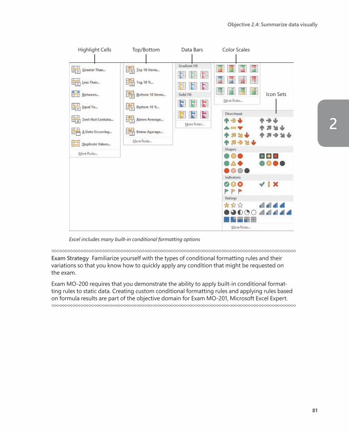
You set up conditional formatting by specifying the condition, which is called a formatting rule. You can select from the following types of rules:

■ Highlight cells Apply formatting to cells that contain data within a specified numeric range, contain specific text, or contain duplicate values.

■ Top/bottom Apply formatting to cells that contain the highest or lowest values in a range.

■ Data bars Fill a portion of each cell corresponding to the relationship of the cell’s data to the rest of the data in the selected range.

■ Color scales Fill each cell with a color point from a two-color or three-color gradient that corresponds to the relationship of the cell’s data to the rest of the data in the selected range.

■ Icon sets Insert an icon from a selected set that corresponds to the relationship of the cell’s data to the rest of the data in the selected range.

81


Highlight Cells Top/Bottom Data Bars Color Scales

Icon Sets

Excel includes many built-in conditional formatting options

Exam Strategy Familiarize yourself with the types of conditional formatting rules and their variations so that you know how to quickly apply any condition that might be requested on the exam.

Exam MO-200 requires that you demonstrate the ability to apply built-in conditional format-ting rules to static data. Creating custom conditional formatting rules and applying rules based on formula results are part of the objective domain for Exam MO-201, Microsoft Excel Expert.

2

82


To quickly apply the default value of a conditional formatting rule

1. Select the data range you want to format.

2. Click the Quick Analysis button that appears in the lower-right corner of the selection (or press Ctrl+Q) and then click Data Bars, Color Scale, Icon Set, Greater Than, or Top 10% to apply the default rule and formatting.

The Quick Analysis menu provides easy access to default conditional formatting

To format font color and cell fill in the selected data range based on a specified condition

1. On the Home tab, in the Styles group, click the Conditional Formatting button.

2. In the Conditional Formatting list, point to Highlight Cell Rules or Top/Bottom Rules, and then click the type of condition you want to specify.

3. In the dialog box, specify the parameters of the condition, click the formatting combination you want, and then click OK.

To apply formatting based on the relationship of values in the selected data range

➜ In the Conditional Formatting list, point to Data Bars, Color Scales, or Icon Sets, and then click the formatting option you want.

83


To remove conditional formatting from selected cells

➜ In the Conditional Formatting list, point to Clear Rules, and then click Clear Rules from Selected Cells or Clear Rules from Entire Sheet.

➜ Open the Conditional Formatting Rules Manager dialog box, click the rule, click Delete Rule, and then click OK.

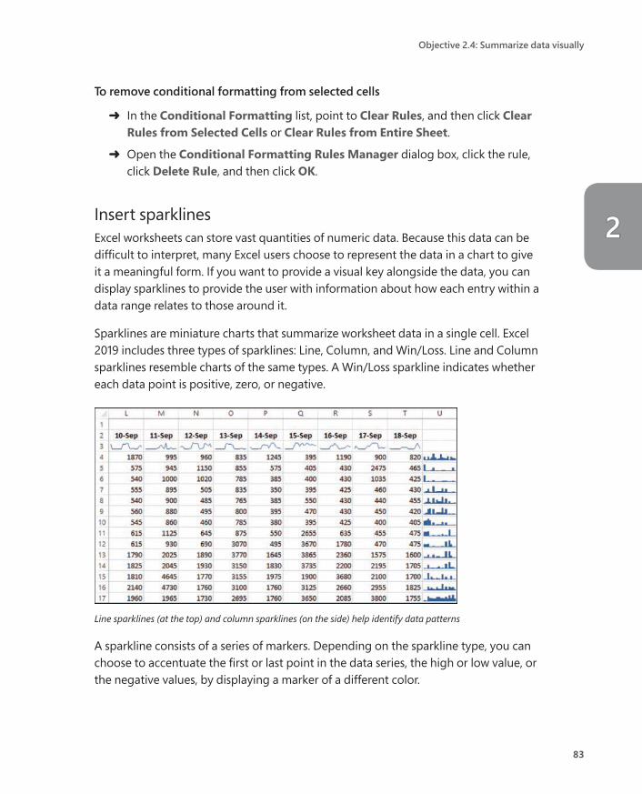
Insert sparklinesExcel worksheets can store vast quantities of numeric data. Because this data can be difficult to interpret, many Excel users choose to represent the data in a chart to give it a meaningful form. If you want to provide a visual key alongside the data, you can display sparklines to provide the user with information about how each entry within a data range relates to those around it.

Sparklines are miniature charts that summarize worksheet data in a single cell. Excel 2019 includes three types of sparklines: Line, Column, and Win/Loss. Line and Column sparklines resemble charts of the same types. A Win/Loss sparkline indicates whether each data point is positive, zero, or negative.

Line sparklines (at the top) and column sparklines (on the side) help identify data patterns

A sparkline consists of a series of markers. Depending on the sparkline type, you can choose to accentuate the first or last point in the data series, the high or low value, or the negative values, by displaying a marker of a different color.

2

84


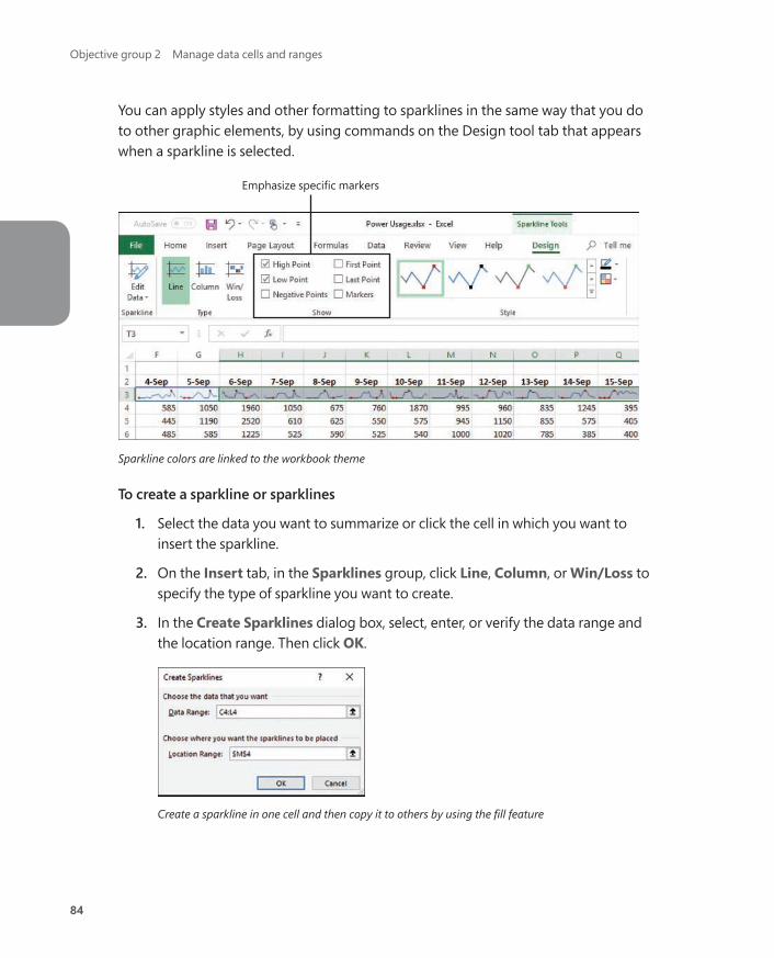
You can apply styles and other formatting to sparklines in the same way that you do to other graphic elements, by using commands on the Design tool tab that appears when a sparkline is selected.

Emphasize specific markers

Sparkline colors are linked to the workbook theme

To create a sparkline or sparklines

1. Select the data you want to summarize or click the cell in which you want to insert the sparkline.

2. On the Insert tab, in the Sparklines group, click Line, Column, or Win/Loss to specify the type of sparkline you want to create.

3. In the Create Sparklines dialog box, select, enter, or verify the data range and the location range. Then click OK.

Create a sparkline in one cell and then copy it to others by using the fill feature

85


To enhance a selected sparkline

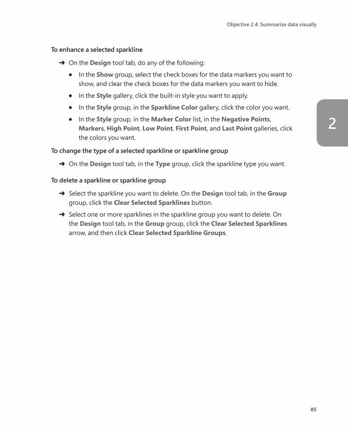
➜ On the Design tool tab, do any of the following:

● In the Show group, select the check boxes for the data markers you want to show, and clear the check boxes for the data markers you want to hide.

● In the Style gallery, click the built-in style you want to apply.

● In the Style group, in the Sparkline Color gallery, click the color you want.

● In the Style group, in the Marker Color list, in the Negative Points, Markers, High Point, Low Point, First Point, and Last Point galleries, click the colors you want.

To change the type of a selected sparkline or sparkline group

➜ On the Design tool tab, in the Type group, click the sparkline type you want.

To delete a sparkline or sparkline group

➜ Select the sparkline you want to delete. On the Design tool tab, in the Group group, click the Clear Selected Sparklines button.

➜ Select one or more sparklines in the sparkline group you want to delete. On the Design tool tab, in the Group group, click the Clear Selected Sparklines arrow, and then click Clear Selected Sparkline Groups.

2


86


➤ Open the Excel_2-4 workbook. On the Order Details worksheet, use conditional formatting to do the following to all the values in the Extended Price column:

❑ Apply the 3 Arrows (Colored) icon set. (Keep the default settings.)

❑ Add Blue data bars to the column. (Keep the default settings.)

❑ Fill all cells in the column that contain values greater than $100 with Yellow.

➤ On the JanFeb worksheet, do the following:

❑ Insert a row below the times. In that row, summarize the data for each hour by using a Column sparkline.

❑ Apply the Colorful #4 sparkline style.

❑ Accentuate the First Point and Last Point data markers.

➤ On the MarApr worksheet, do the following:

❑ In column P, summarize the data for each day of March by using a Line sparkline.

❑ Apply the Orange, Sparkline Style Accent 6, Darker 25% style.

❑ Display all the data markers without placing emphasis on any specific type of data marker.


87

Objective group 3

The skills tested in this section of the Microsoft Office Specialist exam for Microsoft Excel 2019 relate to creating tables. Specifically, the following objectives are associated with this set of skills:

3.1 Create and format tables3.2 Modify tables3.3 Filter and sort table data

An Excel table is a named object that has functionality beyond that of a simple data range. Some table functionality, such as the ability to sort and filter on columns, is also available for data ranges. Useful table functionality that is not available for data ranges includes the automatic application of formatting, the automatic copying of formulas, and the ability to perform the following actions:

■ Quickly insert column totals or other mathematical results.

■ Search for the named table object.

■ Expose the named table object in a web view.

■ Reference the table or any table field by name in a formula.

This chapter guides you in studying methods of creating and modifying tables, applying functional table formatting, and filtering and sorting data that is stored in a table.

Manage tables and table data

3

88

Objective group 3 Manage tables and table data

Objective 3.1: Create and format tables

Create an Excel table from a cell rangeThe simplest way to create a table is by converting an existing data range. If you don’t already have a data range, you can create a blank table and then add data to populate the table.

When you create a table from an existing data range, you choose the table format you want, and then Excel evaluates the data range to identify the cells that are included in the table and any functional table elements such as table header rows.

Excel evaluates the data range that contains the active cell

Each built-in table format you choose has specific functional elements built in to it, such as a header or banded (alternating) row formatting. You can choose the options you want to show on the table style thumbnails or modify the table options after you create the table.

Header formatting Banded row formatting

Choose from 60 preconfigured formatting combinations based on theme colors

89


Excel assigns a name to each table you create, based on its order of creation in the workbook (Table1, Table2, and so on). You can change the table name to one that makes it more easily identifiable (such as Sales_2019, Students, or Products).

IMPORTANT Names must begin with a letter or an underscore character. A name cannot begin with a number.

See Also For more information about naming and renaming tables, see “Objective 2.3: Define and reference named ranges.”

To convert a data range to a table of the default style

1. Click anywhere in the data range.

2. On the Insert tab, in the Tables group, click Table. Excel selects the surrounding data and displays the Create Table dialog box.

Collapse dialog box

You can enter or select the table content

3. Verify that the cell range in the Where is the data for your table box is the cell range you want to convert to a table. If it isn’t, do either of the following:

● Correct the cell range in the dialog box by changing the letters and numbers.

● Click the Collapse Dialog Box button to the right of the cell range, drag to select the cell range you want, and then click the Expand Dialog Box button to return to the full dialog box.

4. If you want to use the top row of the cell range as the table header row, verify that the My table has headers check box is selected.

5. In the Create Table dialog box, click OK.

3

90


To convert a data range to a table and select the table style

1. Click anywhere in the data range.

2. On the Home tab, in the Styles group, click Format as Table, and then click the table style you want.

3. In the Format As Table dialog box, do the following, and then click OK:

a. Verify that the cell range in the Where is the data for your table box is the cell range you want to convert to a table. If it isn’t, do either of the following:

● Correct the cell range in the dialog box by changing the letters and numbers.

● Click the Collapse Dialog Box button to the right of the cell range, drag to select the cell range you want, and then click the Expand Dialog Box button to return to the full dialog box.

b. If you want to use the top row of the cell range as the table header row, verify that the My table has headers check box is selected.

To create an empty table

1. Select the cells in which you want to create the table.

Tip If you select only one cell, Excel creates a two-cell table with one cell designated for the header and one for the content.

2. On the Home tab, in the Styles group, click Format as Table, and then click the table style you want.

3. In the Format As Table dialog box, click OK.

To select a table

➜ In the worksheet, do either of the following:

● Point to the upper-left corner of the table. When the pointer changes to a diagonal arrow, click once to select the table.

● Drag to select all cells of the table.

➜ Click the Name box located at the left end of the formula bar to display a list of named objects, and then click the table.

91


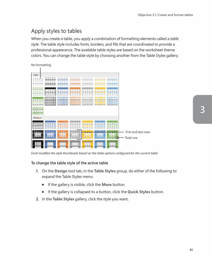
Apply styles to tablesWhen you create a table, you apply a combination of formatting elements called a table style. The table style includes fonts, borders, and fills that are coordinated to provide a professional appearance. The available table styles are based on the worksheet theme colors. You can change the table style by choosing another from the Table Styles gallery.

First and last rows

No formatting

Total row

Excel modifies the style thumbnails based on the table options configured for the current table

To change the table style of the active table

1. On the Design tool tab, in the Table Styles group, do either of the following to expand the Table Styles menu:

● If the gallery is visible, click the More button.

● If the gallery is collapsed to a button, click the Quick Styles button.

2. In the Table Styles gallery, click the style you want.

3

92


To clear formatting from the active table

➜ From the Design tool tab, expand the Table Styles menu, and then do either of the following:

● In the upper-left corner of the Light section of the gallery, click the None thumbnail.

● At the bottom of the menu, click Clear.

➜ Select the table. On the Home tab, in the Editing group, click Clear, and then click Clear Formats.

Convert a table to a cell rangeIf you want to remove the table functionality from a table—for example, so you can work with functionality that is available only for data ranges and not for tables—you can easily convert a table to text. Simply converting the table doesn’t remove any table formatting from the table; you can retain the formatting or clear it.

See Also For information about applying and clearing table formatting, see “Objective 3.2: Modify tables.” For information about functionality that is specific to data ranges, see “Objective 2, Manage data cells and ranges.”

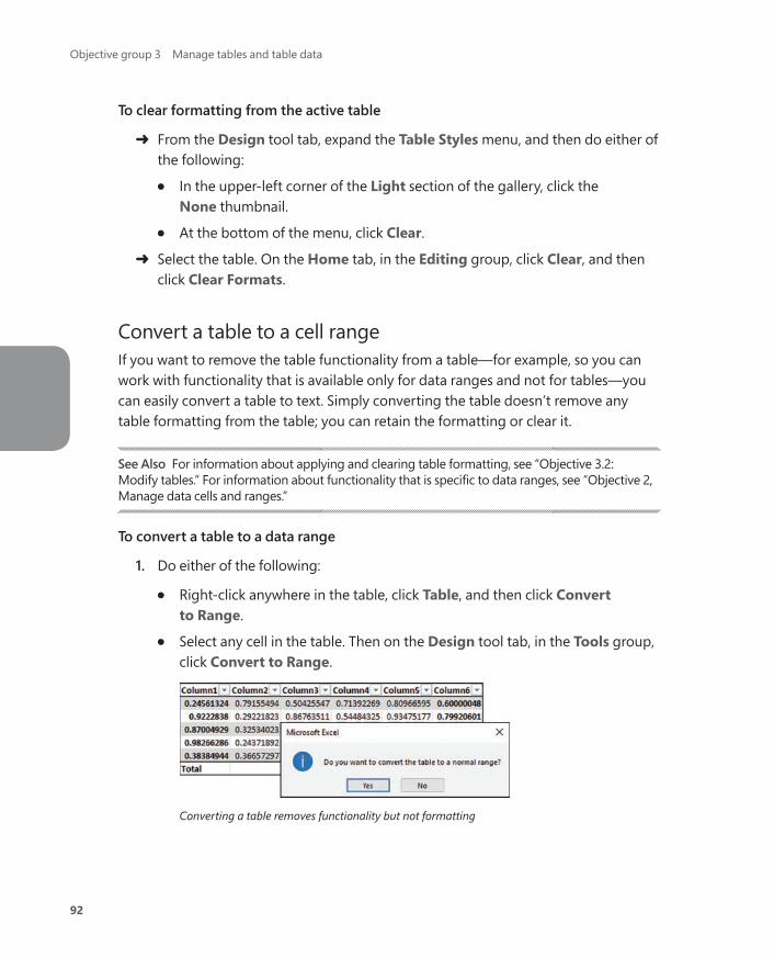
To convert a table to a data range


● Right-click anywhere in the table, click Table, and then click Convert to Range.

● Select any cell in the table. Then on the Design tool tab, in the Tools group, click Convert to Range.

Converting a table removes functionality but not formatting

93


2. In the Microsoft Excel dialog box prompting you to confirm that you want to convert the table to a range, click Yes.

To remove table formatting from a data range

1. Select the data range.

2. On the Home tab, in the Editing group, click Clear and then Clear Formats.

3


94


➤ Open the Excel_3-1 workbook. On the 2019 Sales worksheet, do the following:

❑ Convert the data range B2:M23 to a table that includes a header row and uses Table Style Medium 16.

➤ On the 2020 Sales worksheet, do the following:

❑ Change the table style to Table Style Medium 19.

➤ On the Bonuses worksheet, do the following:

❑ Convert the table to a data range.

❑ Remove the table formatting from the data range.


95

Objective 3.2: Modify tables


Add or remove table rows and columnsInserting, deleting, or moving rows or columns in a table automatically updates the table formatting to gracefully include the new content. For example, adding a column to the right end of a table extends the formatting to that column, and inserting a row in the middle of a table that has banded rows updates the banding. You can modify the table element selections at any time.

To insert table rows and columns

➜ To add a column to the right end of a table, click in the cell to the right of the last header cell, enter a header for the new column, and then press Enter.

➜ To insert a single column within a table, do either of the following:

● Click a cell to the left of which you want to insert a column. On the Home tab, in the Cells group, click the Insert arrow, and then click Insert Table Columns to the Left.

● Select a table column to the left of which you want to insert a column (or select at least two contiguous cells in the column), and then in the Cells group, click the Insert button.

➜ To insert multiple columns within a table, select the number of columns that you want to insert, and then in the Cells group, click the Insert button.

➜ To insert a row at the bottom of the table, click in any cell in the row below the last table row, enter the text for that table cell, and then press Tab.

➜ To insert a row within the table, do either of the following:

● Click a cell above which you want to insert a row. On the Home tab, in the Cells group, click the Insert arrow, and then click Insert Table Rows Above.

● Select a table row above which you want to insert a column (or select at least two contiguous cells in the row), and then in the Cells group, click the Insert button.

➜ To insert multiple rows in a table, select the number of rows that you want to insert, and then in the Cells group, click the Insert button.

3

96


To move rows within a table

1. Select the table row(s) you want to move. (Do not select worksheet cells outside of the table.)

2. Point to the left edge of the selection until the cursor changes to a four-headed arrow.

3. Drag the selection to the new location (indicated by a thick green insertion bar).

Or

1. Select the worksheet row(s) that contain the table rows you want to move.

2. Point to the top or bottom edge of the selection until the cursor changes to a four-headed arrow.

3. Hold down the Shift key and drag the row to the new location (indicated by a thick gray insertion bar). Then release the Shift key.

Or

1. Select the worksheet row(s) that contain the table rows you want to move, and then cut the selection to the Clipboard.

2. Select the worksheet row above which you want to move the cut row or rows.


● On the Home tab, in the Cells group, click the Insert arrow, and then click Insert Cut Cells.

● Right-click the selected column, and then click Insert Cut Cells.

To move columns within a table

1. Select the table column(s) you want to move. (Do not select worksheet cells outside of the table.)

2. Point to the top of the selection until the cursor changes to a four-headed arrow.

3. Drag the selection to the new location (indicated by a thick green insertion bar).

Or

1. Select the worksheet column(s) that contain the table columns you want to move.

97


2. Point to the left or right edge of the selection until the cursor changes to a four-headed arrow.

3. Hold down the Shift key and drag the column(s) to the new location (indicated by a thick gray insertion bar). Then release the Shift key.

Or

1. Select the worksheet column(s) that contain the table columns you want to move, and then cut the selection to the Clipboard.

2. Select the worksheet column to the left of which you want to move the cut col-umn or columns.


● On the Home tab, in the Cells group, click the Insert arrow, and then click Insert Cut Cells.

● Right-click the selected column, and then click Insert Cut Cells.

To delete table rows and columns

➜ Select one or more (contiguous) cells in each row or column you want to delete. On the Home tab, in the Cells group, click the Delete arrow, and then click Delete Table Rows or Delete Table Columns.

➜ Right-click a cell in the row or column you want to delete, click Delete, and then click Table Columns or Table Rows.

Configure table style optionsThe table style governs the appearance of standard cells, special elements, and functional table elements, including the following:

■ Header row These cells across the top of the table are formatted to contrast with the table content, require an entry, and look like column titles, but are also used to reference fields in formulas.

■ Total row These cells across the bottom of the table are formatted to con-trast with the table content. They do not require an entry, but clicking in any cell displays a list of functions for processing the numeric contents of the table column. These include Average, Count, Count Numbers, Max, Min, Sum, StdDev, and Var, and a link to the Insert Function dialog box from which any function can be inserted in the cell.

3

98


Table element formatting is designed to make table entries or fields easier to differentiate, and include an emphasized first column, emphasized last column, banded rows, and banded columns.

Configure formatting and functional options in the Table Style Options group

To enable row-specific table functionality

➜ On the Design tool tab, in the Table Style Options group, do any of the following:

● To designate that the first row contains labels that identify the content below them, select the Header Row check box.

● To add a calculation row at the bottom of a table, select the Total Row check box.

● To hide or display filter buttons (arrow buttons) in the table header, clear or select the Filter Button check box.

Tip Excel automatically adds filter buttons when you format a data range as a table. The filter buttons are adjacent to the right margin of each table header cell. If table columns are sized to fit the column headers and you turn on filter buttons, the filter buttons might overlap the table header text until you resize the column.

99


To apply contrasting formatting to specific table elements

➜ On the Design tool tab, in the Table Style Options group, do any of the following:

● To alternate row cell fill colors, select the Banded Rows check box.

● To alternate column cell fill colors, select the Banded Columns check box.

● To emphasize the content of the first table column (for example, if the column contains labels), select the First Column check box.

● To emphasize the content of the last table column (for example, if the column contains total values), select the Last Column check box.

Exam Strategy Whenever you are instructed to apply consistent formatting to a table, do so using the table formatting commands, not the standard cell formatting commands, so the formatting will persist when the table expands.

To configure the function of a Total row

1. Click any cell of the Total row to display an arrow.

2. Click the arrow to display the functions that can be performed in the cell.

Modify a Total row to perform other mathematical functions

3. In the list, click the function you want to perform in the cell.

4. To perform the same function in all cells of the row, copy the cell formatting to the rest of the row.

3


100


➤ Open the Excel_3-2 workbook, and on the Sales worksheet, do the following:

❑ Configure the table style options to format alternating rows with different fill colors.

❑ Configure the table style options to emphasize the first column of the table.

❑ Move the July column so that it is between the June and August columns.

❑ Move the Linda, Max, and Nancy rows at one time so that they are between the Kay and Olivia rows.

❑ Insert a table row for a salesperson named Raina between the Quentin and Steve rows.

❑ Insert a column named Dec between the Nov and Year columns.

❑ Add a total row to the table.

❑ Change the total row name from Total to Average.

❑ Modify the cells in the Average row to calculate the average sales for each month and for the year.

❑ Delete the Year column from the table.


101

Objective 3.3: Filter and sort table data

Objective 3.3: Filter and sort table dataYou can easily sort and filter content in an Excel table. Sorting sets the order of the content, and filtering displays only rows containing entries that match the criteria you choose.

Filtered rows Sorted Sort and filter options Filtered

In a large data table, locate meaningful data by sorting and filtering the table content

Filter tablesYou can filter a table by the content of one or more columns. You can filter to include or exclude rows that contain an exact match of a column entry, that contain specific text, or that have a specific font color. Filters can include wildcards such as ? (a question mark) to represent any single character or * (an asterisk) to represent a series of characters.

3

102


To filter a table to match a specific column entry

1. Click the filter button in the header of the column by which you want to filter the table.

2. At the top of the list of column entries, clear the (Select All) check box, and then select the check boxes of the items you want to display. Then click OK.

Tip You can enlarge the menu to display more options by dragging the handle in the lower-right corner of the menu.

To specify text filters

1. Click the filter button in the header of the column by which you want to filter the table, click Text Filters, and then click Equals, Does Not Equal, Begins With, Ends With, Contains, or Does Not Contain.

2. In the Custom AutoFilter dialog box, enter one or more filter criteria, and then click OK.

Custom filters can use two different criteria

To specify number filters

1. Click the filter button in the header of the column by which you want to filter the table, click Number Filters, and then click Equals, Does Not Equal, Greater Than, Greater Than Or Equal To, Less Than, Less Than Or Equal To, or Between.

2. In the Custom AutoFilter dialog box, enter one or more filter criteria, and then click OK.

103


To remove a filter

➜ In the table header, click the filter button, and then click Clear Filter From “Column”.

To remove all filters from the active table

➜ On the Home tab, in the Editing group, click Sort & Filter, and then click the active Filter command or click Clear.

➜ Press Ctrl+Shift+L.

Sort tablesYou can sort or filter on one column at a time by using the commands on the menu that appears when you click the filter button at the top of the column, or you can configure a multilevel sort from the Sort dialog box.

A multilevel sort provides a method of displaying different views of large amounts of data

By default, Excel assumes that the first row in the worksheet contains column headings and does not include it in the sort. It also assumes that you want to sort by the values in the table cells. You can sort values numerically or alphabetically in ascending or descending order. Standard sort orders are from A to Z for text, from smallest to largest for numbers, and from oldest to newest for dates. You can optionally sort by other features of the data range, including cell color, font color, and cell icon. These options are particularly useful in conjunction with conditional formatting.

3

104


You can also specify whether entries starting with uppercase and lowercase letters should be sorted separately and the orientation of the sort (whether you want to sort columns or rows).

Tip You can sort a table by the content of hidden columns within that table.

To sort a table by the values in one column

➜ At the right end of the column header, click the filter button, and then click the sort order you want.

To sort the active table by multiple columns


● On the Home tab, in the Editing group, click the Sort & Filter button, and click Custom Sort.

● Click any cell in the range to be sorted, and then on the Data tab, in the Sort & Filter group, click the Sort button.

2. In the Sort dialog box, click the first column you want in the Sort by list. Then click the criteria by which you want to sort in the Sort on list. Finally, click the order you want in the Order list.

Tip The options in the Sort dialog box change if you select a Color or Icon option in the Sort On list.

3. Click Add Level, and repeat step 2 for the second column. Repeat this step for additional columns.

4. Click OK.

To change the sort order

➜ In the Sort dialog box, set the order for each of the sorting criteria.

➜ In the table header, click the active sort button to reverse the sort order.


105


➤ Open the Excel_3-3 workbook, and on the Bonuses worksheet, do the following:

❑ Filter the table to display only the bonuses that were more than $2,500.00.

➤ On the Products worksheet, do the following:

❑ Sort the data by category (from A to Z) and, within each category, by unit price (from lowest to highest).

❑ Sort the data in descending order by category (from Z to A) and, within each category, by product name (from A to Z).


This page intentionally left blank

107

Objective group 4

The skills tested in this section of the Microsoft Office Specialist exam for Microsoft Excel 2019 relate to the application of functions and formulas. Specifically, the following objectives are associated with this set of skills:

4.1 Insert references in formulas4.2 Calculate and transform data by using functions4.3 Format and modify text by using functions

Simple formulas and more complex functions provide the means to interpret raw data stored in a workbook in meaningful ways. They also provide a useful structure for processing information. You can increase the consistency and reliability of information by using formulas to calculate, evaluate, and express data.

You can calculate the data on a worksheet based on data in other areas of the workbook and in other workbooks. Excel maintains referential relationships when you move data or modify the data storage structure.

This chapter guides you in studying ways of referencing cells and ranges of cells both absolutely and relatively in formulas, and using formulas to sum and average cell values and count cells. It also guides you in processing data that meets specific conditions, and in manipulating text by using formulas.

Perform operations by using formulas and functions

4

108

Objective group 4 Perform operations by using formulas and functions

Objective 4.1: Insert references in formulas

Insert relative, absolute, and mixed referencesFormulas in an Excel worksheet usually involve functions performed on the values contained in one or more other cells on the worksheet (or on another worksheet). A reference that you make in a formula to the contents of a worksheet cell is either a relative reference, an absolute reference, or a mixed reference. It is important to understand the difference and know which to use when creating a formula.

A relative reference to a cell takes the form A1. When you copy or fill a formula from the original cell to other cells, a relative reference changes to maintain the relationship between the cell containing the formula and the referenced cell. For example, copying a formula that refers to cell A1 one row down changes the A1 reference to A2; copying the formula one column to the right changes the A1 reference to B1.

An absolute reference takes the form $A$1. The dollar sign indicates an absolute reference to the column or row designator that follows it. When you copy or fill a formula from the original cell to other cells, an absolute reference does not change—regardless of the relationship to the referenced cell, the reference stays the same.

The customer discount is calculated by using an absolute reference to the discount percentage

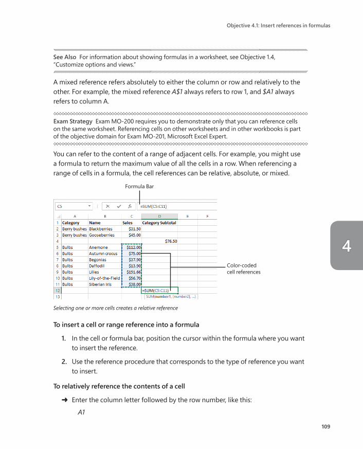
109


See Also For information about showing formulas in a worksheet, see Objective 1.4, “Customize options and views.”

A mixed reference refers absolutely to either the column or row and relatively to the other. For example, the mixed reference A$1 always refers to row 1, and $A1 always refers to column A.

Exam Strategy Exam MO-200 requires you to demonstrate only that you can reference cells on the same worksheet. Referencing cells on other worksheets and in other workbooks is part of the objective domain for Exam MO-201, Microsoft Excel Expert.

You can refer to the content of a range of adjacent cells. For example, you might use a formula to return the maximum value of all the cells in a row. When referencing a range of cells in a formula, the cell references can be relative, absolute, or mixed.

Color-codedcell references

Formula Bar

Selecting one or more cells creates a relative reference

To insert a cell or range reference into a formula

1. In the cell or formula bar, position the cursor within the formula where you want to insert the reference.

2. Use the reference procedure that corresponds to the type of reference you want to insert.

To relatively reference the contents of a cell

➜ Enter the column letter followed by the row number, like this:

A1

4

110


To relatively reference the contents of a range of cells

➜ Enter the upper-left cell of the range and the lower-right cell of the range, separated by a colon, like this:

A1:B3

➜ Drag to select the cell range and insert a relative reference to it.

To absolutely reference the contents of a cell

➜ Precede the column letter and row number by dollar signs, like this:

$A$1

➜ Enter the relative reference, click in or select the reference, and then press F4.

To absolutely reference the contents of a range of cells

➜ Enter the upper-left cell of the range and the lower-right cell of the range, separated by a colon, and precede each column letter and row number by dollar signs, like this:

$A$1:$B$3

➜ Enter the relative range reference, select the range, and then press F4.

Reference named cell ranges and tables in formulasCoverage of Objective 2.3 includes information about naming and renaming cell ranges and tables. A primary reason for naming objects is so that you can easily reference them in formulas. When you compose a formula from the formula bar, named objects appear in a drop-down list as you enter the first characters of the name. You can select the object you want to reference from the list to avoid spelling errors.

Excel makes it easy to reference named objects and ranges

To reference a named range or table in a formula

1. In the formula, begin typing the range name or table name.

2. In the list that appears, select the named object you want to reference in the formula.


111

Objective 4.1 practice tasksThe practice file for these tasks is in the MOSExcel2019\Objective4 practice file folder. The folder also contains result files that you can use to check your work.

➤ Open the Excel_4-1 workbook, display the Multiplication Table worksheet, and do the following:

❑ Create a formula in cell B2 and copy the formula to the other cells in the range B2:K11 to complete the multiplication table of the numbers 1 through 10. Use mixed referencing to ensure that the formula works when copied.

➤ On the Sales By Category worksheet, do the following:

❑ In cell C7, calculate the Carnivorous sales total, using an absolute cell range reference. Then copy the formula to D7 so it returns the same result.

❑ In cells D17, D24, and D28, calculate the sales total for each category by using a relative cell range reference.

❑ In cell D29, use the simplest method to create a formula that returns the total sales for the four categories.


112


Objective 4.2: Calculate and transform data by using functionsFormulas in Excel can be made up of values that you enter, values that you reference (cell references, named ranges, named objects), mathematical operators, and the functions that ultimately structure and control the formula. A function can be thought of as a service provided by Excel to do a specific task. That task might be to perform a mathematical operation, to make a decision based on specific factors, or to perform an action on some text. A function is always indicated by the function name followed by a set of parentheses (for example, the SUM() function).

For most functions, arguments (variables) inside the parentheses either tell the function what to do or identify values for the function to work with. An argument can be a value that you enter, a cell reference, a range reference, a named range, a named object, or even another function. The number and type of arguments vary depending on which function you’re using. Many functions allow optional arguments; these are indicated in function descriptions by square brackets. For example, =SUM(number1,[number2], [number3]) indicates that the SUM() function requires one number but accepts additional numbers. It is important to understand the syntax of common functions and to be able to correctly enter the function arguments. Fortunately, you don’t have to memorize anything; the Formula AutoComplete feature leads you through the process of selecting the correct function name and entering the required arguments in the correct syntax.

Perform calculations by using the SUM(), AVERAGE(), MIN(), and MAX() functionsThe following table describes the purpose of each of the functions that you can use to calculate data from a range of cells, and the types of arguments the functions accept.

Function Purpose Arguments

SUM() Returns the total of the cell values number1,number2,…,number255

AVERAGE() Returns the average of the cell values number1,number2,…,number255

MIN() Returns the minimum value within the set

number1,number2,…,number255

MAX() Returns the maximum value within the set

number1,number2,…,number255

113

Objective 4.2: Calculate and transform data by using functions

Each of these functions takes up to 255 numeric arguments, which can be a number entered directly in the formula, a text representation of a number (a number inside of quotation marks), a cell reference, a range reference, or a named reference. The function ignores any cells that contain text that can’t be translated to a number, that are empty, or that contain an error.

You can enter arguments directly in the formula structure, through a dialog box interface, by clicking to select cells, or by dragging to select ranges.

Arguments for the AVERAGE() function

Probably the most common formula used in Excel, and certainly the simplest to understand, is the SUM() function. The SUM() function returns the total value of a set of numbers. Rather than individually adding the values of all the cells you want to total, you can use the SUM function to perform this task.

Tip The results of the AVERAGE, COUNT, and SUM functions appear by default on the status bar when you select multiple cells (contiguous or separate) that contain numeric values. You can optionally display the Numerical Count, Minimum, and Maximum values.

To sum values

➜ In the cell or formula bar, enter the following formula, including up to 255 numbers, which can be in the form of cell references, a data range, or specific numbers:

=SUM(number1,[number2],[number3]…)

4

114


➜ On the Formulas tab, in the Function Library group, click the AutoSum arrow (not the button), and then click Sum. Select or enter the numeric arguments you want to sum, and then press Enter.

➜ In the Function Library group, click the AutoSum button (not the arrow) and press Enter to accept the logical range of values selected by Excel (the range immediately above or to the left of the active cell).

➜ Click the AutoSum button. Click or drag to select the input values you want (press and hold Ctrl to select multiple cells and ranges). Then press Enter.

Or

1. On the Formulas tab, in the Function Library group, click Math & Trig, and then click SUM to open the Function Arguments dialog box displaying prompts for the SUM() function.

2. In the Number1 box, enter or select the first number.

3. In the Number2 box and each subsequent box, enter or select the additional numbers up to a total of 255 arguments.

4. In the Function Arguments dialog box, click OK.

To average values in a data range

➜ In the cell or formula bar, enter the following formula, including up to 255 cell references or data ranges:

=AVERAGE(number1,[number2],[number3]…)

➜ In the Function Library group, click the AutoSum arrow, and then click Average. Select or enter the cells you want to average, and then press Enter.

Or

1. In the Function Library group, click More Functions, click Statistical, and then click AVERAGE to open the Function Arguments dialog box displaying prompts for the AVERAGE() function.

2. In the Number1 box, enter or select the first data range.

3. In the Number2 box and each subsequent box, enter or select additional data ranges up to a total of 255 arguments.


115


To return the lowest value in a data range


=MIN(number1,[number2],[number3]…)

➜ In the Function Library group, click the AutoSum arrow, and then click Min. Select or enter the cells you want to evaluate, and then press Enter.

Or

1. In the Function Library group, click More Functions, click Statistical, and then click MIN to open the Function Arguments dialog box displaying prompts for the MIN() function.




To return the highest value in a data range


=MAX(number1,[number2],[number3]…)

➜ In the Function Library group, click the AutoSum arrow, and then click Max. Select or enter the cells you want to evaluate, and then press Enter.

Or

1. In the Function Library group, click More Functions, click Statistical, and then click MAX to open the Function Arguments dialog box displaying prompts for the MAX() function.




4

116


Count cells by using the COUNT(), COUNTA(), and COUNTBLANK() functionsThe following table describes the purpose of each of the functions that you can use to count data from a range of cells, and the types of arguments the functions accept.

Function Purpose Arguments

COUNT() Returns the number of cells that contain numeric values

value1,value2,…,value255

COUNTA() Returns the number of cells that contain any content (are not empty)

value1,value2,…,value255

COUNTBLANK() Returns the number of empty cells range

Each of these functions takes up to 255 numeric arguments, either numbers or values, as follows:

■ An argument specified as a number can be a number that is entered directly in the formula, a text representation of a number (a number inside of quotation marks), a cell reference, a range reference, or a named reference. The function ignores any cells that contain text that can’t be translated to a number, that are empty, or that contain an error.

■ An argument specified as a value can be any type of value. For example, the COUNT() function will evaluate the specified cells and return the count of only those that contain values it identifies as numbers, whereas the COUNTA() function will evaluate the cells and return the count of those that contain any content (are not blank).

Arguments for the COUNTA() function

117


To count cells containing numeric values


=COUNT(value1,[value2],[value3]…)

➜ In the Function Library group, click the AutoSum arrow, and then click Count Numbers. Select or enter the cells you want to count, and then press Enter.

Or

1. In the Function Library group, click More Functions, click Statistical, and then click COUNT.

2. In the Function Arguments box, do the following, and then click OK.

● In the Value1 box, enter or select the first data range.

● In the Value2 box and each subsequent box, enter or select additional data ranges up to a total of 255 arguments.

To count non-empty cells


=COUNTA(value1,[value2],[value3]…)

Or

1. In the Function Library group, click More Functions, click Statistical, and then click COUNTA.

2. In the Function Arguments box, do the following, and then click OK.

● In the Value1 box, enter or select the first data range.

● In the Value2 box and each subsequent box, enter or select additional data ranges up to a total of 255 arguments.

To count empty cells


=COUNTBLANK(range)

4

118


Or

1. In the Function Library group, click More Functions, click Statistical, and then click COUNTBLANK.

2. In the Function Arguments box, enter or select the data range in the Range box, and then click OK.

Perform conditional operations by using the IF() functionYou can use a formula to display specific results when certain conditions are met. To do so, you create a formula that uses conditional logic—specifically, the IF() function or one of its variations.

Exam Strategy Exam MO-200 requires that you be able to demonstrate the use of the IF() function. Variants such as the SUMIF(), SUMIFS(), COUNTIF(),COUNTIFS(), AVERAGEIF(), and AVERAGEIFS() functions are part of the objective domain for Microsoft Office Specialist Exam MO-201, Microsoft Excel Expert.

A formula that uses conditional logic evaluates a specific condition and then returns one of two results based on whether the logical test evaluates as TRUE or FALSE.

The correct syntax for the IF() function is IF(logical_test,value_if_true,value_if_false). For example, the following formula evaluates a student’s grade in cell D4 and returns Pass if the grade is 70 or above and Fail if the grade is less than 70:

=IF(D4<70,”Fail”,”Pass”)

When using the IF() function, the logical test must be one that can have only a true or false result.

Tip The IF() function in Excel is equivalent to an IF…THEN…ELSE function in a computer program.

The logical test and the results can include text strings or calculations. Enclose text strings within the formula in quotation marks.

Exam Strategy You can nest multiple functions so that Excel evaluates multiple conditions before returning a result. You can add logical tests to a conditional formula by using the AND(), OR(), and NOT() functions. Nested functions and custom conditional formats are part of the objective domain for Microsoft Office Specialist Exam MO-201, Microsoft Excel Expert.

119


To return a value based on a conditional test

➜ In the cell or formula bar, enter the following formula, where logical_test is the condition that must be met, value_if_true is the value the formula returns if the condition is met, and value_if_false is the value the formula returns if the condition is not met:

= IF(logical_test,value_if_true,value_if_false)

Or

1. On the Formulas tab, in the Function Library group, click Logical, and then click IF to open the Function Arguments dialog box displaying prompts for the IF() function.

2. In the Logical_test box, enter a pass/fail condition.

3. In the Value_if_true box, enter the value the formula will return if the condition is met. To return a text string, enclose it in quotes.

4. In the Value_if_false box, enter the value the formula will return if the condition is not met.


4


120


➤ Open the Excel_4-2 workbook. On the Sales By Region worksheet, do the following:

❑ In cell A18, create a formula that returns the number of non-empty cells in the cell range named Season.

❑ In cell D5, create a formula that returns the average Sales value for the Fall season.

❑ In cell D9, create a formula that returns the maximum Sales value for the Spring season.

❑ In cell D13, create a formula that returns the minimum Sales value for the Summer season.

❑ In cell G2, create a formula that returns the average value in the cell range named Sales.

❑ In cell F5, use the IF function to display the text “Excellent sales season!” if D5 is higher than G2, and otherwise leaves the cell blank.


121

Objective 4.3: Format and modify text by using functions


Select text by using the LEFT(), MID(), and RIGHT() functionsYou can use the formulas shown in the following table to return portions of cell content based on position.

Function Description

LEFT() Returns the leftmost character or characters of a text string

MID() Returns a specific number of characters from a text string, starting at the position you specify

RIGHT() Returns the rightmost character or characters of a text string

The LEFT(), MID(), and RIGHT() functions count each character in the specified text string. The LEFT() and RIGHT() functions take the following arguments:

■ text (required) The text string to be evaluated by the formula.

■ num_chars (optional) The number of characters to be returned. If num_chars is not specified, the function returns one character.

The syntax for the LEFT() and RIGHT() functions is:

LEFT(text,num_chars)

RIGHT(text,num_chars)

For example, the formula =LEFT(Students[@[Last Name]],1) returns the first letter of the student’s last name.

The MID() function takes the following arguments:

■ text (required) The text string to be evaluated by the formula.

■ start_num (required) The position from the left of the first character you want to extract. If start_num is greater than the number of characters in the text string, the function returns an empty string.

■ num_chars (required) The number of characters to be returned. If num_chars is not specified, the function returns one character.

4

122


The syntax for the MID() function is:

MID(text,start_num,num_chars)

The MID() function returns a specific number of characters from a text string

To return one or more characters from the left end of a text string

➜ In the cell or formula bar, enter the following formula, where text is the source text and num_chars is the number of characters you want to return:

=LEFT(text,num_chars)

Or

1. On the Formulas tab, in the Function Library group, click Text, and then click LEFT to open the Function Arguments dialog box displaying prompts for the LEFT() function.

2. In the Text box, enter or select the source text.

3. In the Num_chars box, enter the number of characters you want to return.


To return one or more characters from within a text string

➜ In the cell or formula bar, enter the following formula, where text is the source text, start_num is the character from which you want to begin returning characters, and num_chars is the number of characters you want to return:

=MID(text,start_num,num_chars)

Or

1. On the Formulas tab, in the Function Library group, click Text, and then click MID to open the Function Arguments dialog box displaying prompts for the MID() function.


123


3. In the Start_num box, enter the character from which you want to begin returning characters.



To return one or more characters from the right end of a text string

➜ In the cell or formula bar, enter the following formula, where text is the source text and num_chars is the number of characters you want to return:

=RIGHT(text,num_chars)

Or

1. On the Formulas tab, in the Function Library group, click Text, and then click RIGHT to open the Function Arguments dialog box displaying prompts for the RIGHT() function.




Format text by using the UPPER(), LOWER(), and PROPER() functionsYou can use the formulas shown in the following table to return case-modified text. This is useful when you want to make data from a variety of sources consistent.


UPPER() Converts text to uppercase

LOWER() Converts text to lowercase

PROPER() Capitalizes the first letter of each word in a text string

The UPPER(), LOWER(), and PROPER() functions each take only one argument: the text string to be processed. The syntax of the functions is:

UPPER(text)

LOWER(text)

PROPER(text)

4

124


To convert a text string to uppercase

➜ In the cell or formula bar, enter the following formula, where text is the source text:

=UPPER(text)

Or

1. On the Formulas tab, in the Function Library group, click Text, and then click UPPER.

2. In the Function Arguments dialog box, enter or select the source text that you want to convert to uppercase, and then click OK.

To convert a text string to lowercase


=LOWER(text)

Or

1. On the Formulas tab, in the Function Library group, click Text, and then click LOWER.

2. In the Function Arguments dialog box, enter or select the source text that you want to convert to lowercase, and then click OK.

To capitalize each word of a text string


=PROPER(text)

Or

1. On the Formulas tab, in the Function Library group, click Text, and then click PROPER.

2. In the Function Arguments dialog box, enter or select the source text that you want to convert to lowercase, and then click OK.

125


Count characters by using the LEN() and LENB() functionsThe LEN() function returns the number of characters within a specific cell (including spaces). This may be useful if you’re developing text content in an Excel workbook; similar functionality is provided by the Word Count utility in Microsoft Word.

The LENB() function provides the same results for double-byte character set (DBCS) languages such Chinese, Japanese, and Korean.

The LEN() and LENB() functions each take only one argument: the text string to be processed. The syntax of the functions is:

LEN(text)

LENB(text)

Combine text by using the CONCAT() and TEXTJOIN() functionsYou can use the formulas shown in the following table to join the contents of multiple cells.


CONCAT() Concatenates up to 253 text components into one string

TEXTJOIN() Concatenates up to 252 text components separated by a specified delimiter

IMPORTANT The CONCATENATE() function that was available in earlier versions of Excel has been replaced by the CONCAT() function. CONCATENATE() is available in Excel 2019 for backward compatibility but might not be available in future versions of Excel.

The CONCAT() and TEXTJOIN() functions can be very useful when working with text data. Using these functions, you can merge existing content from cells in addition to content that you enter in the formula.

The syntax for the CONCAT() function is:

CONCAT(text1,[text2],...)

4

126


The [text] arguments can be cell references, table column references, or text enclosed in double quotes.

For example, this formula returns a result such as Smith, John: Grade 5.

= CONCAT(Table1[@[Last Name]],”, “,Table1[@[First Name]],”: Grade “, Table1[@Grade])

Tip You can use the ampersand (&) operator to perform the same process as the CONCAT() function. For example, =A1&B1 returns the same value as =CONCAT(A1,B1).

The TEXTJOIN() function is similar to CONCAT(), but also inserts a delimiter between the text strings you’re concatenating, and has the option to exclude empty arguments from the concatenated results. The syntax for the TEXTJOIN() function is:

TEXTJOIN(delimiter,ignore_empty,text1,[text2],…)

The delimiter is required; it can be a space or any character string enclosed in double quotes. You can have only one delimiter per formula.

The ignore_empty argument must be either TRUE or FALSE and specifies whether to return any empty results.

For example, this formula returns the name Joan Elizabeth Lambert:

TEXTJOIN(“ “,TRUE,”Joan”,”Elizabeth”,”Lambert”)

To join multiple text strings in one cell

➜ In the cell or formula bar, enter the following formula, including up to 253 text strings, which can be in the form of cell references or specific text enclosed in quotation marks:

=CONCAT(text1,[text2],[text3]…)

Or

1. On the Formulas tab, in the Function Library group, click Text, and then click CONCAT.

2. In the Function Arguments dialog box, in the Text1 box and each subsequent box, enter or select a cell reference or enter specific text. Then click OK.

127


To join and delimit multiple text strings in one cell

➜ In the cell or formula bar, enter the following formula, including up to 255 text strings, which can be in the form of cell references or specific text enclosed in quotation marks:

=TEXTJOIN(delimiter,ignore_empty,text1,[text2],[text3]…)

Or

1. On the Formulas tab, in the Function Library group, click Text, and then click TEXTJOIN to open the Function Arguments dialog box displaying prompts for the TEXTJOIN() function.

2. In the Delimiter box, enter or select the character or characters you want the formula to insert between the text strings.

3. In the Ignore_empty box, enter TRUE if you want to omit empty arguments from the results or FALSE to return empty results between delimiters.

4. In the Text1 box and each subsequent box, enter or select a cell reference or enter specific text.


4

147

IndexSYMBOLS& (ampersand) operator, 126

Aabsolute references, 108–110Accessibility Checker, 38–39accessibility issues

alternative text in charts, 144–145inspecting workbooks for, 38–39

activatingfooter area, 24header area, 23

adding commands to Quick Access Toolbar, 28alignment of text, changing, 66–68alternative file formats, saving workbooks, 47–50alternative text

in charts, 144–145for hyperlinks, creating, 16

ampersand (&) operator, 126AND() function, 118area charts, 130Auto Fill, 55–57AVERAGE() function, 112–115AVERAGEIF() function, 118AVERAGEIFS() function, 118axes (of charts)

switching, 139–140types of, 140

Bbackward compatibility

maintaining, 42saving workbooks, 47

bar charts, 130box & whisker charts, 130

Ccalculations with functions, 112–115category axis, 140

cells. See also rangescounting, 116–118filling based on adjacent columns, 61–62formatting

based on content, 80–83copying to other cells, 73–74with number formats, 70–73with styles, 69–70

with hyperlinks, selecting, 12hyperlinks to, creating, 15inserting, 63merging, 65–66pasting contents, special paste options,

57–61styles, 69–70text

alignment/orientation/indentation, 66–68wrapping, 68–69

unmerging, 66changing. See editingcharacters, counting, 125chart sheets, moving charts to, 135chart titles, 140charts

creating, 132–135editing

content, 137–140elements, 140–141

formattingwith alternative text, 144–145with layouts and styles, 143–144

moving to chart sheets, 135switching axes, 139–140types of, 130–132

clearingprint area, 44table formatting, 92

closing header/footer area, 24color scales, 80column charts, 130columns

deleting, 19, 62filling cells based on, 61–62freezing, 30–31

148

columns

inserting, 19, 62repeating when printing, 45–46in tables

deleting, 97inserting, 95–97moving, 96–97

transposing, 61width, changing, 19–21

combination charts, 132combining text, 125–127commands on Quick Access Toolbar

adding, 28removing, 28reordering, 28separating, 28

Compatibility Checker, 40–42compatibility issues, inspecting workbooks for,

40–42CONCAT() function, 125–127CONCATENATE() function, 125conditional formatting, 80–83conditional operations, 118–119converting

ranges to tables, 88–90tables to ranges, 92–93

copying formatting to other cells, 73–74COUNT() function, 116–118COUNTA() function, 116–118COUNTBLANK() function, 116–118COUNTIF() function, 118COUNTIFS() function, 118counting

cells, 116–118characters, 125

currency number format, applying, 72–73custom headers/footers, creating, 22–23custom page size, setting, 18customizing Quick Access Toolbar, 26–29

Ddata bars, 80data calculation with functions, 112–115data labels, 140data ranges. See rangesdecimal number format, applying, 73default number format, applying, 71deleting

rows/columns, 19, 62

in tables, 97sparklines, 85

delimited text filesimporting data from, 2–7saving workbooks, 48

delimiters, 2displaying. See viewingDocument Inspector, 36–38

Eediting

chartscontent, 137–140elements, 140–141

column width, 19–21headers/footers, 24hyperlinks, 16page setup options, 18–19print area, 43–44row height, 19–21splits in window, 32text alignment/orientation/indentation,

66–68workbook properties, 33–34

Ffile formats, saving workbooks, 47–50files, creating hyperlinks to, 13, 14–15filling

cells based on adjacent columns, 61–62series, 54–57

filter buttons in tables, 98filtering tables, 101–103Flash Fill, 61–62folders, creating hyperlinks to, 13footers, 21–24

activating area, 24closing area, 24configuring options, 24creating custom, 22–23editing, 24inserting standard, 22

Format Painter, 73–74formatting

cellsbased on content, 80–83copying to other cells, 73–74

149

margins, changing

with number formats, 70–73with styles, 69–70

chartswith alternative text, 144–145with layouts and styles, 143–144

filling series without, 57pasting, 60with Quick Analysis tool, 132ranges, removing, 93searching for, 10tables with styles, 91–92, 97–99text, 123–124text alignment, 66–68

formatting rules, 80formulas

referencesto named objects, 110types of, 108–110

viewing, 33freezing rows/columns, 30–31functions, 112

calculating data, 112–115combining text, 125–127conditional operations, 118–119counting cells, 116–118counting characters, 125formatting text, 123–124selecting text, 121–123

funnel charts, 130

GGet Data, 3Go To dialog box, 10–11Go To Special dialog box, 10–11

Hheaders, 21–24

activating area, 23closing area, 24configuring options, 24creating custom, 22–23editing, 24inserting standard, 22

height of rows, changing, 19–21hidden properties, inspecting workbooks for,

36–38hiding chart elements, 141

highlight cells rule, 80histogram charts, 130hyperlinks

creating, 11–16editing, 16removing, 16selecting cells with, 12

Iicon sets, 80IF() function, 118–119ignoring

images by screen readers, 145print area, 44

images, ignoring by screen readers, 145importing data into workbooks, 2–7indentation of text, changing, 68Insert Hyperlink dialog box, 12inserting

cells, 63data into ranges, 60headers/footers, standard, 22references into formulas, 108–110rows/columns, 19, 62

in tables, 95–97sparklines, 83–85

inspecting workbooksaccessibility issues, 38–39compatibility issues, 40–42hidden properties/personal information,

36–38

Llayouts for charts, 143–144LEFT() function, 121–123legends (on charts), 140LEN() function, 125LENB() function, 125line charts, 131links. See hyperlinksLOWER() function, 123–124

Mmacro-enabled workbooks, 47map charts, 131margins, changing, 18–19

150

MAX() function

MAX() function, 112–115merging cells, 65–66MID() function, 121–123MIN() function, 112–115mixed references, 108–110modifying. See editingmoving

charts to chart sheets, 135Quick Access Toolbar, 29table columns, 96–97table rows, 96

NName Manager, 76named cells, navigating to, 10–11named objects

hyperlinks to, creating, 15referencing, 78, 110

named ranges, 76–78naming tables, 76, 89navigating within workbooks, 10–11NOT() function, 118number filters for tables, 102number formats, 70–73

OOR() function, 118orientation of text, changing, 68

Ppage orientation, changing, 19page setup options, editing, 18–19Paste Special, 57–61pasting

cell contents, special paste options, 57–61formatting, 60

PDF format, 48percentage number format, applying, 72personal information, inspecting workbooks

for, 36–38pie charts, 131Power Query Editor, 4–5pre-addressed email messages, creating, 16print area

clearing, 44editing, 43–44

ignoring, 44printing

scaling content, 46workbooks, 42–43worksheet elements, 44–46worksheets, 42–44

PROPER() function, 123–124properties of workbooks, editing, 33–34

QQuick Access Toolbar

customizing, 26–29moving, 29resetting, 29

Quick Analysis tool, 132

Rradar charts, 131ranges, 53

convertingto tables, 88–90tables to, 92–93

defining as print area, 43–44formatting, removing, 93inserting data, 60named ranges, 76–78navigating to, 10–11referencing in formulas, 110removing from print area, 44series, filling, 54–57

references, types of, 108–110referencing named objects, 78, 110relative references, 108–110removing

commands from Quick Access Toolbar, 28conditional formatting, 83hyperlinks, 16range formatting, 93ranges from print area, 44splits in window, 32table filters, 103

renaming tables, 78reordering commands on Quick Access

Toolbar, 28repeating rows/columns when printing, 45–46resetting Quick Access Toolbar, 29RIGHT() function, 121–123

151

viewing

rowsdeleting, 19, 62freezing, 30–31height, changing, 19–21inserting, 19, 62repeating when printing, 45–46in tables

deleting, 97inserting, 95–97moving, 96

transposing, 61

Ssaving workbooks, alternative file formats,

47–50scaling print content, 46scatter charts, 131screen readers, ignoring images, 145searching in workbooks, 9–10selecting

cells with hyperlinks, 12tables, 90text, 121–123

separating commands on Quick Access Toolbar, 28

series, filling, 54–57series axis, 140sorting tables, 103–104sparklines

deleting, 85inserting, 83–85

special paste options, 57–61splitting worksheets in window, 32standard page size, setting, 18stock charts, 131styles

cells, 69–70charts, 143–144tables, 91–92

configuring options, 97–99SUM() function, 112–115SUMIF() function, 118SUMIFS() function, 118sunburst charts, 131surface charts, 131switching

chart axes, 139–140views, 29–30

Ttables

converting to ranges, 92–93creating from ranges, 88–90filter buttons, 98filtering, 101–103naming, 76, 89referencing in formulas, 110renaming, 78rows/columns

deleting, 97inserting, 95–97moving, 96–97

selecting, 90sorting, 103–104styles, 91–92

configuring options, 97–99templates, saving workbooks, 48text

alignment of, changing, 66–68combining, 125–127counting characters, 125formatting, 123–124indentation of, changing, 68orientation of, changing, 68searching for, 9selecting, 121–123wrapping, 68–69

text filters for tables, 102Text Import Wizard, 3TEXTJOIN() function, 125–127top/bottom rule, 80transposing rows/columns, 61treemap charts, 131

Uunfreezing rows/columns, 31unmerging cells, 66UPPER() function, 123–124

Vvalue axis, 140values (of cells), pasting, 60viewing

chart elements, 141formulas, 33

152

views

viewsin separate windows, 32switching, 29–30

Wwaterfall charts, 131webpages

hyperlinks to, creating, 12saving workbooks, 47

width of columns, changing, 19–21workbook elements, navigating to, 10–11workbooks

dataimporting, 2–7searching, 9–10

hyperlinks to, creating, 13–14inspecting

for accessibility issues, 38–39for compatibility issues, 40–42for hidden properties/personal

information, 36–38navigating within, 10–11printing, 42–43

properties, editing, 33–34Quick Access Toolbar, creating specific, 29saving, alternative file formats, 47–50views in separate windows, 32

worksheet elements, printing, 44–46worksheets

hyperlinks to, creating, 15page footer area

activating, 24closing, 24

page header areaactivating, 23closing, 24

printing, 42–44scaling, 46splitting in window, 32views, switching, 29–30

wrapping text, 68–69

XX Y charts, 131XML formats, 47XPS format, 48

ScoutAutomatedPrintCode - pearsoncmg.com

Documents

Transcript of ScoutAutomatedPrintCode - pearsoncmg.com