ScientiVc Computing mit Python

Andreas PritschetInstitut für Experimentelle und Angewandte Physik

Universität RegensburgJanuary 27, 2013

Contents

1 Introduction 21.1 Literature . . . . . . . . . . . . . . 21.2 What is Python? . . . . . . . . . . 31.3 Some initial remarks . . . . . . . 3

2 Basics 52.1 First steps . . . . . . . . . . . . . 52.2 The interactive Shell . . . . . . . . 62.3 Operators . . . . . . . . . . . . . 72.4 Variables & Data types . . . . . . 7

2.4.1 Numeric data types . . . . 72.4.2 Sequences . . . . . . . . . 82.4.3 Strings . . . . . . . . . . . 102.4.4 Special Operations on

Sequences . . . . . . . . . 112.4.5 Type conversion . . . . . . 12

2.5 Control Structures . . . . . . . . . 132.5.1 Conditional statements . 142.5.2 Loops . . . . . . . . . . . 152.5.3 pass & del . . . . . . . . . 18

2.6 Input & Output . . . . . . . . . . 192.7 Functions . . . . . . . . . . . . . . 232.8 Modules – Importing . . . . . . . 26

3 Advanced – Part 1 283.1 List Comprehensions . . . . . . . 283.2 Object Orientation . . . . . . . . 293.3 Modules – Writing & Documen-

tation . . . . . . . . . . . . . . . . 343.4 Exception Handling . . . . . . . . 36

4 Advanced – Part 2 414.1 Threading . . . . . . . . . . . . . 41

4.1.1 Threads . . . . . . . . . . 414.1.2 Events & Locks . . . . . . 44

4.2 Queue . . . . . . . . . . . . . . . 494.3 Graphical User Interfaces with Tk 51

4.3.1 Geometry Manager – pack 534.3.2 Geometry Manager – grid 534.3.3 Widgets – Input . . . . . 544.3.4 Events . . . . . . . . . . . 57

5 Modules for science 615.1 NumPy . . . . . . . . . . . . . . . 62

5.1.1 Arrays . . . . . . . . . . . 625.1.2 Masked Arrays . . . . . . 675.1.3 Matrices . . . . . . . . . . 715.1.4 Polynomials . . . . . . . . 73

5.2 SciPy . . . . . . . . . . . . . . . . 755.2.1 Derivation . . . . . . . . . 775.2.2 Fourier Transforms . . . . 805.2.3 Integral . . . . . . . . . . 84

5.3 MatPlotLib . . . . . . . . . . . . . 885.3.1 Plotting in 1D . . . . . . . 885.3.2 Plotting in 2D . . . . . . . 91

5.4 Mayavi . . . . . . . . . . . . . . . 955.4.1 Mesh types . . . . . . . . 965.4.2 Plotting in 3D . . . . . . . 98

6 Exercises 1066.1 The Basics . . . . . . . . . . . . . 1066.2 Advanced I . . . . . . . . . . . . . 1066.3 Advanced II . . . . . . . . . . . . 1076.4 Numerical Computations . . . . . 107

1 INTRODUCTION

XKCD.com

1 Introduction1.1 Literature• Python Scripting for Computational Science Langtangen, Hans Petter; Springer Verlag

• OXcial Python Documentation

• Tutorial on Threads Programming with Python MatloU, Norman und Hsu, Francis

• Documentation of MatPlotLib

• Documentation of NumPy/SciPy

• OXcial Mayavi Documentation

• SciPy Conference 2008 presentation of Mayavi Prabhu Ramachandran and Gaël Varoquaux

• An Introduction to Tkinter Lundh, Fredrik

• How to Think Like a Computer Scientist (Python) JeUrey Elkner, Allen B. Downey and ChrisMeyers

• Style Guide for Python Code Guido van Rossum und Barry Warsaw

• The History of Python Blog of Guido v. Rossum and Greg Stein

This is a small selection of resources. There is much more available on the Net and in form ofbooks.

2

1 INTRODUCTION

1.2 What is Python?Python is ...

• ... a modern open-source scripting language. Source codes are not compiled before execution;it is interpreted in "real time".

• Traditionally scripting languages are used for smaller tasks, e.g. executing a series of shellcommands (shell script on Linux, batch script on Windows), but thanks to code optimizationthe Python interpreter is quite powerful.

• Contrary to traditional scripting languages Python is object-orientated and shows modernexception handling features.

• ... is a so-called "glue language" as it can call external programs and incorporate e.g. Cprograms and libraries.

Pro

• The Python language is designed to match the syntax of spoken languages. Thus writingPython code gets as simple as telling another person to do something. This gets even easieras there is an enormous supply of well-documented modules.

• Because it is open-source it is available for almost all operating systems, but portability ofscripts will be limited when using operating system speciVc commands.

Contra

• Python scripts can be fast, but a well written and compiled program will always be faster.

• As Python has a more human-compatible syntax the focus of the language is not on micro-processor programming and stuU like that. If you want to do that using Python, it might geta bit tricky.

1.3 Some initial remarksWhat do you need to work in the Linux CIP-Pool?

• First of all you need a Linux-Account. If you do not have one, contact Wolfgang Pulinaor Michael Hartung.

• You might proVt from previous programming experience.

• You should not be afraid of using the Linux shell.

What to do to get a certiVcate

• To get a certiVcate you are asked to do a project within of two weeks.

• It does not have to be long, but it should show a certain level of complexity, e.g.: If yourscript asks for user input, perform tests whether the input is valid or use Python’s exceptionhandling capabilities.

• You should not forget documentating your project.

• Afterwards mail it and your name to andreas.hasenkopf@physik.uni-regensburg.de

3

1 INTRODUCTION

Installation

• Installing Python and its modules is as simple as possible. You can use binary installers orjust copy&paste script Vles.

• Please note, that we are working on Debian Linux, which does not come with the most recentsoftware!

– Python: 2.5.2

– NumPy: 1.1.0

– SciPy: 0.6.0

– Matplotlib: 0.98.1

• For writing script Vles you simply need a text editor. Classical command line editors arevi(m) and nano. More comfortable, graphical editors are kate, idle, blueVsh and even more.

4

2 BASICS

2 Basics2.1 First steps

Listing 1: Hello World (hw1.py)# ! / u s r / b i n / env python

import math

print " He l lo , World ! "print " s i n ( 1 ) = " , math . s i n ( 1 )

• Python shows similarities in the choice of key words and other language elements. But inPython as many syntax elements as possible are omitted.

– Expressions are not followed by a ";". They are Vnished by the end of line.

– Code blocks are not encapsulated in "{...}". Code blocks consist of consecutive expres-sions with the same or a higher indentation level. But be careful: a tab is wider than asimple space, but they both count as one indentation.

• Comments begin with "#"

• Like C or C++ Python has a limited set of instructions which is extended by additional mod-ules. In order to import a module one uses the import statement. Notice how an elementfrom this module is referenced!

• Executing Python scripts

– ./hw1.py: this is the typical way a Linux user would start a script (regardless of itslangauge). In order for this to work the line starting with #! is required (On Windowssystems this line is treated as a comment) and the Vle has to be executable.

– python hw1.py: Calling the Python interpreter directly to run the script

– Some editors oUer a button to run scripts!

Listing 2: Output (hw1.out)Hel lo , World !s i n ( 1 ) = 0 . 8 4 1 4 7 0 9 8 4 8 0 8

• In order to enable computers/programs to display meaningful texts they need a so calledcharacter encoding. The biggest problem is, that diUerent operating systems use diUerentencodings and diUerent languages (e.g. English, Cyrillic, Chinese, ...).

• Independent on the encoding of the operating system Python interprets its scripts usingASCII, the quasi-standard understood by every computer in the world. But not every char-acter is known in ASCII (see Listing 5).

• Therefore Python can read source codes using other encodings, too. Another very goodchoice is UTF8, which is also quite universal. To change the encoding one adds an extra lineas shown in Listing 4.

5

2 BASICS

• For more information on character encodings see Python Lib. Reference and Python Tutorial.

Listing 3: Example (coding1.py)# ! / u s r / b i n / env python

print " Ha l l o F l öhe "

Listing 4: Example (coding2.py)# ! / u s r / b i n / env python# −∗− c o d i n g : u t f 8 −∗−

print " Ha l l o F l öhe "

Listing 5: Output of coding1.pyF i l e " cod ing1 . py " , l i n e 3

Syn t a xE r r o r : Non−ASCII c h a r a c t e r ’ \ xc3 ’ in f i l e cod ing1 . py on l i n e 3 , butno encod ing d e c l a r e d ; s ee h t tp : / /www. python . org / peps / pep−0263 . html

for d e t a i l s

Listing 6: Output of coding2.pyHa l l o F l öhe

2.2 The interactive Shell• The shell is started by calling "python" plainly or by "python -i a_script.py", which executesthe script before starting the shell.

• The shell is an ideal place for experiments (code is executed immediately after input) andoUers full documentation on modules, functions, etc.

• After statements requiring a following indented block (e.g. if) the shell prompts for anotherline until an empty line is entered.

Listing 7: Interactive Shell (pshell.out)Python 2 . 5 . 2 ( r 2 5 2 : 6 0 9 1 1 , Oct 5 2008 , 1 9 : 2 9 : 1 7 )[GCC 4 . 3 . 2 ] on l i n u x 2Type " he lp " , " c opy r i gh t " , " c r e d i t s " or " l i c e n s e " for more i n f o rma t i on

.>>> a = 3 ∗ 5 + 4>>> a19>>> print a19>>>

• All return values are printed to the shell, if not stated otherwise.

• To get the full documentation (identical to documentation on python.org) one needs thesestatements

6

2 BASICS

help() Shows documentation on an object.

dir() Lists the contents of a module.

Listing 8: Interactive Shell (dirbsp.out)>>> import math>>> d i r ( math )[ ’ __doc__ ’ , ’ __name__ ’ , ’ __package__ ’ , ’ acos ’ , ’ acosh ’ , ’ a s i n ’ , ’ a s i nh ’ ,

’ a tan ’ , ’ a tan2 ’ , ’ atanh ’ , ’ c e i l ’ , ’ c opys i gn ’ , ’ cos ’ , ’ cosh ’ , ’ d eg r e e s ’, ’ e ’ , ’ exp ’ , ’ f a b s ’ , ’ f a c t o r i a l ’ , ’ f l o o r ’ , ’ fmod ’ , ’ f r e x p ’ , ’ fsum ’ , ’hypot ’ , ’ i s i n f ’ , ’ i s nan ’ , ’ l d exp ’ , ’ l o g ’ , ’ l o g 10 ’ , ’ l og1p ’ , ’modf ’ , ’p i ’ , ’ pow ’ , ’ r a d i a n s ’ , ’ s i n ’ , ’ s i nh ’ , ’ s q r t ’ , ’ tan ’ , ’ tanh ’ , ’ t r unc ’ ]

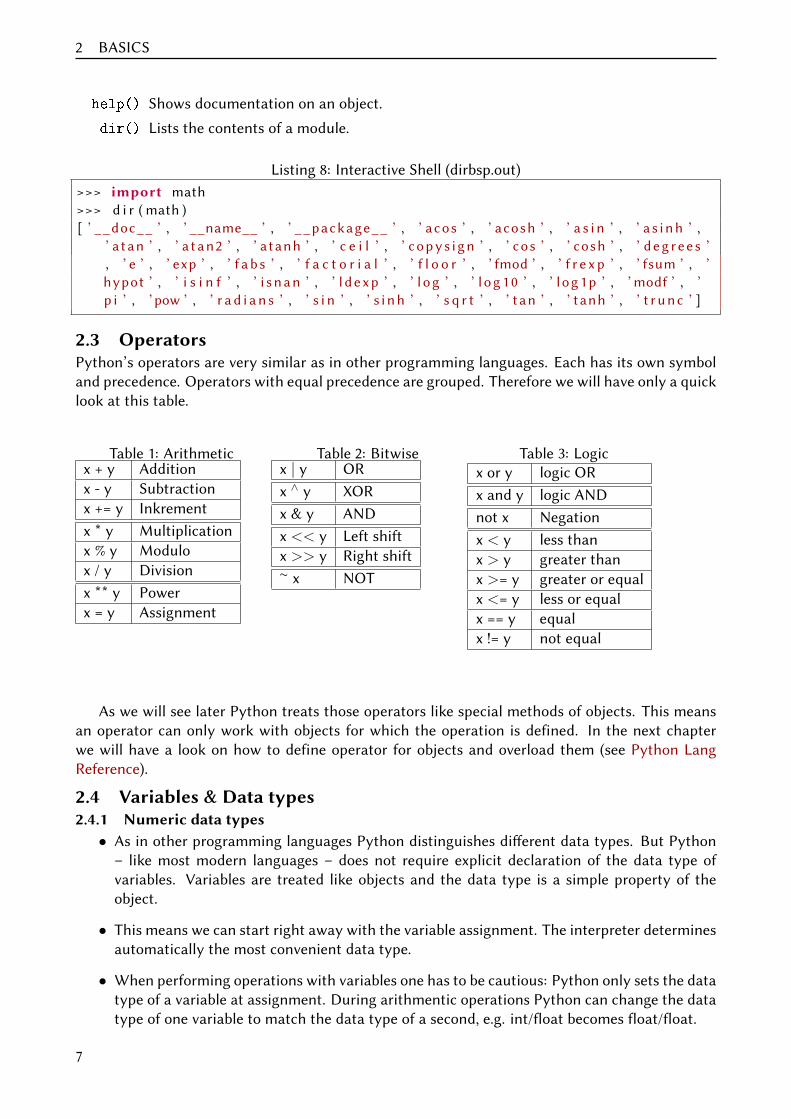
2.3 OperatorsPython’s operators are very similar as in other programming languages. Each has its own symboland precedence. Operators with equal precedence are grouped. Therefore we will have only a quicklook at this table.

Table 1: Arithmeticx + y Additionx - y Subtractionx += y Inkrementx * y Multiplicationx % y Modulox / y Divisionx ** y Powerx = y Assignment

Table 2: Bitwisex | y ORx ∧ y XORx & y ANDx << y Left shiftx >> y Right shift∼ x NOT

Table 3: Logicx or y logic ORx and y logic ANDnot x Negationx < y less thanx > y greater thanx >= y greater or equalx <= y less or equalx == y equalx != y not equal

As we will see later Python treats those operators like special methods of objects. This meansan operator can only work with objects for which the operation is deVned. In the next chapterwe will have a look on how to deVne operator for objects and overload them (see Python LangReference).

2.4 Variables & Data types2.4.1 Numeric data types• As in other programming languages Python distinguishes diUerent data types. But Python– like most modern languages – does not require explicit declaration of the data type ofvariables. Variables are treated like objects and the data type is a simple property of theobject.

• This means we can start right away with the variable assignment. The interpreter determinesautomatically the most convenient data type.

• When performing operations with variables one has to be cautious: Python only sets the datatype of a variable at assignment. During arithmentic operations Python can change the datatype of one variable to match the data type of a second, e.g. int/Woat becomes Woat/Woat.

7

2 BASICS

• Integers: Python internally distinguishes two diUerent kinds of integers: Integers and LongIntegers (only on 64bit systems). The user/programmer does not notice the diUerence.

• Floating point numbers: Python uses 64 bits to save Woats in an exponent-mantissa schemacovering the range: ≈ [±4.9 ∗ 10−324,±1.8 ∗ 10+308]

• Complex numbers: Complex numbers can be written using both mathematical notations,whereby j is the complex unit. In general complex numbers are objects like Woats, but withtwo special attributes: imag and real.

Listing 9: Example: Numerals>>> a = 23>>> b = 2>>> # Two e x p r e s s i o n s i n one l i n e ! !. . . a+b , a∗∗b # a d d i t i o n , power( 2 5 , 5 2 9 )>>> a / b , a / f l o a t ( b ) # d i v i o n by i n t and f l o a t( 1 1 , 1 1 . 5 )>>> z = 2 3 . 1 + 4 j # complex>>> z # z i s an o b j e c t !( 2 3 . 1 0 0 0 0 0 0 0 0 0 0 0 0 0 1+ 4 j )>>> z . r e a l # r e a l p a r t2 3 . 1 0 0 0 0 0 0 0 0 0 0 0 0 0 1>>> z . imag # imag i na r y p a r t4 . 0

2.4.2 Sequences• Sequence is the general term for higher dimensional data structures. They are also knownby the name array.

• Sequences may be of arbitrary complexity and may contain any Python object. Most impor-tant, those objects to not need to be of the same data type!

• List

– Numerical index, Vrst index is "0" (zero)

– Comma separated list of values in square brackets: A = [ 2,5,4,77,43 ]

– Lists are more than simple data containers. Theay are objects with quite a lot methods(siehe help(list)).

– Single elements or sublists of lists can be changed.

• Tuple

– Identical to a list, but it can not be changed after assignment!

– Parenthesis instead of square brackets.

• Dictionary:

– In other contexts known as associative array.

8

2 BASICS

– Comma separated list of key:value pairs in curly brackets: D = { "foo": 12, "bar":

34 }

– The index – or key – may be of the type string, but also integers and Woats are allowed!

– Behaves mostly like a "list with some extra features".

• Strings

– Strings are tuples for "characters", they can not be edited in-place like lists.

– One can perform all operations allowed for tuples on strings, too.

• As we will see in chapter 5 the list of multidimensional data structures will extend for specialkinds of sequences designed for use in numerical mathematics: Array & Matrix.

Listing 10: Example: Operations (bsp3.out)>>> # D e f i n i n g s e q u e n c e s. . . A = ( 1 , 4 . , ’ Ha l l o ’ , 1 + 2 j ) # Tup l e>>> B = [−2 , −3+1 j , ( 1+1 j , 2−3 j ) ] # L i s t>>> C = { " foo " : ’ Ha l l o ’ , " bar " : ’ Welt ’ , 2 3 : ’ Echo ’ } # D i c t i o n a r y>>> A( 1 , 4 . 0 , ’ Ha l l o ’ , ( 1+2 j ) )>>> B[−2 , (−3+1 j ) , ( ( 1 + 1 j ) , (2−3 j ) ) ]>>> # one can r e f e r e n c e s i n g l e e l emen t s. . . # u s i n g c u r l y b r a c k e t s [ ]. . . B [ 2 ] # e l emen t a t p o s i t i o n 2( ( 1 + 1 j ) , (2−3 j ) )>>> # B [ 2 ] i s t h e t h i r d e l emen t and a t u p l e. . . # To r e f e r e n c e e l emen t s o f t h e t u p l e u se e x t r a [ ]. . . B [ 2 ] [ 0 ] . imag , B [ 2 ] [ 0 ] . r e a l( 1 . 0 , 1 . 0 )>>> # one can change l i s t e l emen t s. . . B [ 1 ] = " He l l o ">>> print B[−2 , ’ He l l o ’ , ( 1+1 j , 2−3 j ) ]>>> print B [ 0 : 2 ] # a s l i c e o f B[−2 , ’ He l l o ’ ]

Operations on sequences in Python have in most cases the same behavior as in other languages,but in the other cases the Python syntax is more like the syntax of spoken languages.

Operation Returnsx in s True, if sequence s contains the element x

False, if sequence s does not contain the element xx not in s False, if sequence s contains the element xs + t Joined sequence containing the elements of s and ts * n, n * s Joins n-times the sequence s and returns its[i] i. Element with index/key i of ss[i:j] Sequence/Slice containing elements of s from position i till js[i:j:k] Slice of s as above, but only each kth element between i and jlen(s) Length of smin(s) Smallest element of smax(s) Largest element of s

9

2 BASICS

2.4.3 Strings• Strings are deVned using quotes. In Python one distinguished between two types of strings:string containing line breaks and string wich don’t.

• The latter are deVned using a single (’) or double (") quote at the beginning and end of thestring. In Python those quote characters are equivalent.

• In order to insert a line break in the string the quoting characters are tripled, e.g. """HelloWorld"""

• As strings are quite wide spread and important there also many modules assisting in thehandling and manipulation of strings, z.B.: strings, stringprep, re, ... (see Python LibRef)

• Python oUers string formatting like the printf statement in C/C++. Therefore the modulooperator "%" is used.

Listing 11: Example: Strings (str_bsp.out)>>> a , b = ’ Ha l l o ’ , " Welt ">>> a + ’ ’ + b # J o i n i n g s t r i n g s’ Ha l l o Welt ’>>> # S u b s t r i n g s. . . print a [ 3 ] , a [ 1 : ] , a [ 2 : 4 ]l a l l o l l>>> ( a + ’ ’ + b ) . upper ( ) # c o n v e r t t o upper c a s e’HALLO WELT ’>>> a , b = 1 . 2 3 , 15395>>> c = " Ha l l o # no l i n e break a l l owed

F i l e " < s td in > " , l i n e 1c = " Ha l l o

^Syn t a xE r r o r : EOL while s cann ing s t r i n g l i t e r a l>>> c = " " " Ha l l o # now l i n e b r e a k s may. . . Welt " " " # o c c u r w i t h i n t h e s t r i n g>>> print c’ Ha l l o \ nWelt ’

• In many languages string formatting can only be done in a function like printf known fromC/C++. Python allows this operation at any time.

• Usually one uses a variable’s data type as the convertion type. As we will see in an example,the behavior might get unpredictable.

• The rules and mechanisms for string formatting are identical to C/C++. A formatting rulefollows this scheme:

– "%" – indicates the beginning of the rule

– Mapping key – string which is a key in a dictionary (optional)

– Conversion Wag – additional formatting, e.g. signum, leading zeros (optional)

10

2 BASICS

– Field width – minimal width for the string (optional)

– decimal digits – number of decimal digits to be displayed (optional)

– Conversion type – Target format

Wags types"0" leading zeros ’d’, ’i’ Signed integer"+" leading signum ’e’, ’E’ Exponential Woat"-" left hand side alignment ’f’, ’F’ Decimal Woat

’s’, ’r’ String (calls __str__() or__repr__())

’%’ The character "%"

The formatting rule "%05.2f" % 23.1 would convert the Woating point number into the string"23.10". For full documentation see Python Documentation.

Listing 12: Example: (str_format.out)>>> # S t r i n g f o rm a t t i n g u s i n g d i c t i o n a r y key s. . . d = { " foo " : 1 3 . 2 4 , " bar " : 3 4 , " b l a " : −1e−4 }>>> print " E in Wert %( foo ) 5 . 3 f und noch zwei : %( bar ) 06d und %( b l a ) + 6 . 3 g "

% dEin Wert 1 3 . 2 4 0 und noch zwei : 000034 und −0.0001>>> # S t r i n g f o rm a t t i n g o f an i n t e g e r. . . # d e c ima l d i g i t s a r e c oun t ed bu t no t d i s p l a y e d !. . . print " E in Wert i s t %5 .3 d " % 23E in Wert i s t 023>>> # S t r i n g f o rm a t t i n g w i t h v a l u e s i n a t u p l e. . . print " % .2 f $ f o r a p i e c e o f %s i s way too much ! " % ( 1 2 . 4 , " cheese " )1 2 . 4 0 $ for a p i e c e o f cheese i s way too much !>>> # S t r i n g s can be f o rma t t e d e v e r ywhe r e a t any t ime. . . e i n_we r t = " I ch b in der Wert %08 .3 f " % −23.735>>> print e in_we r tI ch b in der Wert −023 .735

2.4.4 Special Operations on SequencesUsing sequence types you get a variety of methods for handling those objects. For now we willhave only a quick review of some interesting methods of strings and dictionaries.

• Strings

– Testing the string returning a boolean resultendswith isalnum isalphaisdigit islower isspace

isdecimal startswith

– Manipulating the stringcapitalize decode encodeexpandtabs format lower

lstrip partition replaceswapcase translate upper

zVll

– Splitting a string into a tuple: (split)

11

2 BASICS

– Joining a sequence to a string: (join)

• Dictionaries

– Testing whether a key exists.

– Retrieving elements from the dictionary safely.

del d[key] key in d key not in dclear copy get(key)

has_key(key) items() iteritems()iterkeys() itervalues() keys()pop(key) popitem() setdefault(key)update() values()

Listing 13: Example (bsp4.out)>>> l = [ ’ Ha l l o ’ , ’ auch ’ , ’ Welt ’ ]>>> ’ ’ . j o i n ( l )’ Ha l l o auch Welt ’>>> d = { ’ h a l l o ’ : ’ Ha l l o ’ ,. . . ’ we l t ’ : ’ Welt ’ ,. . . ’ h e l l o ’ : ’ He l l o ’ ,. . . ’ wor ld ’ : ’World ’. . . }>>> d . ge t ( ’ h a l l o ’ )’ Ha l l o ’>>> d . ge t ( ’ h o l l a ’ )>>> d [ ’ h o l l a ’ ]T raceback ( most r e c e n t c a l l l a s t ) :

F i l e " < s td in > " , l i n e 1 , in <module >KeyEr ro r : ’ h o l l a ’>>> d . pop ( ’ we l t ’ )’ Welt ’>>> print d{ ’ h a l l o ’ : ’ Ha l l o ’ , ’ h e l l o ’ : ’ He l l o ’ , ’ wor ld ’ : ’World ’ }

2.4.5 Type conversion• As we have seen Python determines the data type of a value during assignment.

• Python does not change the data type of an object on its own.

Listing 14: Example (cast1bsp.out)>>> a , b = 2 , 5>>> print a / b0>>> print 3 / 70>>> print 3 / 7 .0 . 4 2 8 5 7 1 4 2 8 5 7 1>>> print 3 / complex ( 7 )( 0 . 4 2 8 5 7 1 4 2 8 5 7 1 + 0 j )

12

2 BASICS

• In order to convert the data type of a value we have some simple functions:

int() float()

long() complex()

str() repr()

⇒ If a conversion is not possible, there will be an error message ("ValueError").

• Everything is an object, therefor e.g. an integer number is an object of the class "int" with avalue and a series of methods.

• Names of objects (variables, functions, classes, ...) and key words in Python have to complywith this lexical deVnition:

i d e n t i f i e r : : = ( l e t t e r | " _ " ) ( l e t t e r | d i g i t | " _ " ) ∗l e t t e r : : = l owe r c a s e | uppe rcasel owe r ca s e : : = " a " . . . " z "uppe rcase : : = "A" . . . "Z "d i g i t : : = " 0 " . . . " 9 "

• Keyworlds

and del from notas elif global orassert else if passbreak except import printclass exec in raisecontinue Vnally is returndef for lambda trywhile with yield

2.5 Control Structures• Like you may know from other programming languages, loops and if statements are quiteimportant. you can use them as you are used from other languages, but they have someadditional features.

• To deVne a code block, e.g. after an if statement, indentation is used. Lines with the samelevel of indentation are considered to be part of one block.

• As you can see in Listing 15 code blocks may occur within other code blocks. The identiVesthe last line of a code block, if the next line has a lower level of indentation.

⇒ Attentiont! For indentation one can use spaces, tabs or any other withespace characters.Tabs are usually displayed being 4 or 8 spaces wide, but regarding indentation in Python onetab has the same indentation level as one space! Especially during copy & paste you shouldcontrol the indentation levels!

13

2 BASICS

Listing 15: Example (if3bsp.py)# ! / u s r / b i n / env python

i f True : # t r i v i a l , da True immer wahr i s tprint " Ha l l o Welt "s = ( " Ha l l o " , " Welt " , " He l l o " , " World " )i f l e n ( s ) ==1 : # d i e s e Bed ingung i s t immr unwahr

print se l se :

for c in s : # I t e r a t i o n uebe r a l l e E l emen t e von sprint c

Listing 16: Output: if3bsp.pyHa l l o WeltHa l l oWeltHe l l oWorld

2.5.1 Conditional statements• The if-Statement evaluates an expression and executes a following code block if the expres-sion evaluates to be true.

• The key word if is followed by the expression and a colon ":"

• The expression may be any comparing relation or object.

– Relations are evaluated whether they are true or false.

– Objects are evaluated whether their return value is not equal None or 0 (Zero).

⇒ An expression consisting only of an integer is evaluated as True, if its value is not equal0.

• If the expression is true, the block following the if statements is executed, otherwise not.

• If it is not and an elif statement follows the block, the expression following elif is evaluated.

• If no expression was evaluated true by all if and elif statements and an else statement ispresent, the block following this statement is executed.

Listing 17: if1bsp.py# ! / u s r / b i n / env python

a = 102b = 23

i f a == b :print ’ g l e i c h ’

e l i f a < b :print ’ k l e i n e r ’

e l se :print ’ g r o e s s e r ’

14

2 BASICS

Listing 18: if2bsp.py# ! / u s r / b i n / env python

va l u e = 1i f va l u e :

print ’ Das i s t wahr ’e l se :

print ’ Das i s t unwahr ’

2.5.2 Loops• while - Loop

– This statement is used like in any other language.

– The key word is followed by an expression for evaluation and a colon ":".

– The loop is repeated until the expression becomes False.

Listing 19: whilebsp_en.py# ! / u s r / b i n / eny python

name_ l i s t = [ ’ Andi ’ , ’ Andreas ’ , ’ J o s e f ’ , ’ Mart in ’ , ]

l a enge = l en ( name_ l i s t )i = 0

# i n C/C++ t h i s e q u a l s a f o r l oopwhile i < l a enge :

print name_ l i s t [ i ]i += 1

# t h i s l oop doe s no t end e v e rwhile True :

pass

• for - Loop

– This statement behaves diUerent compared to other languages. In Python the for state-ment is only used for iterations on sequences!

– The syntax is comparable to the syntax of a spoken language: for (each) fruit in (the)fruit-basket. In this example, fruit-basket is a sequence and fruit is a variable name,which has not been assigned yet or can be overwritten.

– The code block following a for loop is n times executed, whereby n is the length of thesequence in the for statement.

– During each cycle of the loop one element of th sequence is assigned to the variable.The variable can be altered (deleted, overwritten, etc.) from within the loop, but thesequence can not be altered directly.

– The for loop is Vnished when all elements of he sequence have been assigned. Afterardsthe variable holds the last value assigned to it and is still known outside the loop.

15

2 BASICS

• If one needs an iteration from one integer to another, the function range() can be of greatassistance. This function generates a tuple of integers.

• Terminating loops

break exits the current cycle and aborts the loop.

continue exists the current cycle, but continues the loop.

Listing 20: loopbsp.py# ! / u s r / b i n / env python

s = ’ Ha l l o Welt ’t = [ ’ Ha l l o ’ , ’ Welt ’ , ’ He l l o ’ , ’World ’ , ’ Echo ’ ]

out = [ ]

# For each l e t t e r i n t h e s t r i n gfor c in s :

i f c == ’ e ’ :break

out . append ( c )

print ’ ’ . j o i n ( out )

# s i s 10 c h a r a c t e r s l o n g# f o r each number from 0 t o 9for c in range ( l e n ( s ) ) :

print ’ %03d %c ’ % ( c , s [ c ] )

# For each s t r i n g i n t h e t u p l efor word in t :

print word [ : : − 1 ]word=word [ : : − 1 ]

# Man i pu l a t i n g t h e v a r i a b l e word has no# i n f l u e n c e on t h e e l emen t s o f t h e s e qu en c e !print t

Listing 21: AusgabeHa l l o W000 H001 a002 l003 l004 o005006 W007 e008 l009 t

16

2 BASICS

o l l aHtleWo l l eHdlroWohcE[ ’ Ha l l o ’ , ’ Welt ’ , ’ He l l o ’ , ’World ’ , ’ Echo ’ ]

• One of the most intriguing new designs is the for/while ... else construct; it is an else state-ment following a for statement.

• The else block is executed, if

– Iteration over the sequence has Vnished (for loop)

– Expression turns false (while loop)

• The else block is omitted, if the loop has been terminated using break.

Listing 22: else in loops(elselpbsp.out)>>> for n in range ( 2 , 1 0 ) :. . . for x in range ( 2 , n ) :. . . i f n % x == 0 :. . . print n , ’ e qua l s ’ , x , ’ ∗ ’ , n / x. . . break. . . e l se :. . . # l oop f e l l t h r ough w i t h ou t f i n d i n g a f a c t o r. . . print n , ’ i s a pr ime number ’. . .2 i s a prime number3 i s a prime number4 equa l s 2 ∗ 25 i s a prime number6 equa l s 2 ∗ 37 i s a prime number8 equa l s 2 ∗ 49 equa l s 3 ∗ 3

Listing 23: else in loops(elselp2bsp.out)>>> for i in range ( 3 ) :. . . p = raw_input ( ’ Password : ’ ). . . i f p == ’ geheim ’ :. . . print " Co r r e c t ". . . break. . . e l se :. . . print "Max l o g i n s reached ". . .Password : h a l l oPassword : t e s tPassword : l e e rMax l o g i n s reached

17

2 BASICS

>>> for i in range ( 3 ) :. . . p = raw_input ( ’ Password : ’ ). . . i f p == ’ geheim ’ :. . . print " Co r r e c t ". . . break. . . e l se :. . . print "Max l o g i n s reached ". . .Password : h a l l oPassword : geheimCor r e c t

2.5.3 pass & del• pass Statement

– pass is doing nothing, literaly.

– This statement serves one single purpose: providing an indented line of code, if anindentation is expected, e.g. after a while statement.

⇒ Python does not accept control statements (e.g. if, while) without a subsequent codeblock.

Listing 24: Example: pass (passbsp.out)>>> def i n i t l o g (∗ a rg s ) :. . . pass # Remember t o imp lement t h i s !. . .

>>> while True :. . . pass # Busy−wa i t f o r keyboa rd i n t e r r u p t ( C t r l +C). . .

• del Statement

– Deletes an object and frees the space of memory used by that object.

⇒ Do not call del on a non-existing object: NameError

⇒ Especially when working with huge data sets and/or Threading you should keep countof your objects.

– When deleting a sequence, Vrst the single elements are deleted from left to right.

Listing 25: Example: del (delbsp.out)>>> a = 128>>> a128>>> del a>>> aTraceback ( most r e c e n t c a l l l a s t ) :

F i l e " < s td in > " , l i n e 1 , in <module >NameError : name ’ a ’ i s not de f i n ed>>> a = range ( 0 , 1 5 )>>> a

18

2 BASICS

[ 0 , 1 , 2 , 3 , 4 , 5 , 6 , 7 , 8 , 9 , 1 0 , 1 1 , 1 2 , 1 3 , 14 ]>>> del a [ 3 : 6 ]>>> a[ 0 , 1 , 2 , 6 , 7 , 8 , 9 , 1 0 , 1 1 , 1 2 , 1 3 , 14 ]

2.6 Input & Output• Output using print

– This statement accepts every type of object as input as it is calling the __str__()methodof the object.

– In the simplest cases, print is called with a string or sequence of strings.

– The print statement accepts its argument(s) with or without surrounding parentheses.

• Input using raw_input

– Default method for querying input in the command line.

– The Python script waits until end of line (EOL).

– raw_input accepts one optional string argument: prompting string.

– This function returns the input as a string.

• Input using input

– Identical to raw_input with one diUerence.

– The input is not returned, it is passed to the eval statement, which interprets its argu-ment as Python source code and executes it.

⇒ Do not use unless you are exactly knowing what you are doing.

Listing 26: Example (inout1bsp.py)# ! / u s r / b i n / env python

print ( ’ Beenden mit \ ’ q u i t \ ’ ’ )

while True :wert = raw_input ( ’ E in Wort : ’ )print ’Du has t ge sag t : "% s " ’ % wert

# p r i n t ( ’Du h a s t g e s a g t : "% s " ’ % we r t )

i f wert == ’ qu i t ’ :break

Listing 27: example (inout1bsp.out)>>> x , a = 2 . 3 , " Ha l l o ">>> y = inpu t ( ’ E ingabe : ’ )E ingabe : x + 23>>> print y , a , " Welt " , 892 5 . 3 Ha l l o Welt 89

19

2 BASICS

>>> print a , " Welt " + 89Ha l l oTraceback ( most r e c e n t c a l l l a s t ) :

F i l e " < s td in > " , l i n e 1 , in <module >TypeEr ro r : cannot conca t ena t e ’ s t r ’ and ’ i n t ’ o b j e c t s>>> print a , " Welt " + s t r ( 8 9 )Ha l l o Welt89

• Files are accessed using open(), e.g. file_obj = open(filename, mode). open returns anobject representing the Vle. Using this Vle handler we can perform operations on the Vle.

Modesr readw writea append

• Content of the Vle is read per line by these two methods. Each method returns the line as astring. The last characters are whitespace characters indicating the end of the line, usually(depending on the OS) it is "\n" or "\r\n".

– Read the next one line file_obj.readline()

– Read all lines as a list of strings file_obj.readlines()

• Depending on the chosen mode when calling open the method write() appends text at theend of the existing Vle or appends to a blank Vle, e.g. file_obj.write(a_string).

• Changes to the Vle are only saved, when the close method of the Vle handler is called, e.g.file_obj.close()

Listing 28: Example (inout2bsp.py)# ! / u s r / b i n / env python

f i l e = open ( ’ loremipsum . t x t ’ , ’ r ’ )l i n e = ’ ’i = 0while l e n ( l i n e ) > 0 :

i += 1l i n e = f i l e . r e a d l i n e ( )print ’%3 i %s ’ % ( i , l i n e [ :−1] )

f i l e . c l o s e ( )

f i l e = open ( ’ loremipsum . t x t ’ , ’ r ’ )l i n e s = f i l e . r e a d l i n e s ( )f i l e . c l o s e ( )

l i n e s [ 1 2 ] = l i n e s [ 1 2 ] [ : − 1 ] + ’ " Ha l l o " ’

f i l e = open ( ’ loremipsum . t x t ’ , ’w ’ )f i l e . w r i t e ( ’ \ n ’ . j o i n ( l i n e s ) )f i l e . c l o s e ( )

20

2 BASICS

Listing 29: Example (inoutbsp.py)# ! / u s r / b i n / env python

from date t ime import date

f i l e = open ( ’hw1 . out ’ , ’ r ’ )i n h a l t = f i l e . r e a d l i n e s ( )f i l e . c l o s e ( )

print i n h a l t

datum = s t r ( date . today ( ) )f i l e = open ( datum + ’ . t x t ’ , ’w ’ )f i l e . w r i t e ( ’ \ n ’ . j o i n ( i n h a l t ) + datum )f i l e . c l o s e ( )

• In the beginning the Vle hw1.out contains one line "Hello World!"

• The Vle is opened two times: once for reading and once for writing. As the writing modewould overwrite the content it is saved in the variable inhalt and written to the Vle togetherwith another string afterwards.

• Notice: The method write does not append newline characters at the end of the string likereadline.

Listing 30: Output on Screen[ ’ He l lo , World ! \ n ’ ]

Listing 31: Content of Vle (2008-12-30.txt)Hel lo , World !2008−12−30

• For interacting with other processes we have two modules at hand: os and subprocess.

• The module os oUers a series of simple functions like os.popen().

• os.popen()

– Calls external programs using a "pipe" known from most Unix shells. One can passarguments to a program and retrieve its return value.

– popen() accepts two arguments like open(). The Vrst is the program/process that shallbe executed as a string; this string has to comply with the syntax of the shell of runningOS.

– The second argument is the mode: w, r or a.

– As popen is connect via a pipe its return value is the return value of the executed com-mand. And that is a string.

• subprocess

21

2 BASICS

– subprocess.Popen() is a more sophisticated alternative to os.popen() accepting a vari-ety of parameters. See Python Lib. Ref.

– subprocess oUers a series of convenience functions which are themselves calling Popen()with often needed combinations of parameters:

∗ call(*popenargs, **kwargs) – popenargs is a sequence containing command nameand arguments. This function waits until the command has Vnished and returns astatus code.∗ check_call(*popenargs, **kwargs) – identical to call; additionaly the process is checkedfor potential errors. If an error has occured, Python’s exception handling system istriggered.∗ check_output(*popenargs, **kwargs) – Similar to check_call, but output of the com-mand is returned.

⇒ Detecting errors and exception handling get much easier.

Listing 32: (popen1bsp.py)# ! / u s r / b i n / env python

import os

# ps − r e p o r t s a s n ap s ho t o f t h e c u r r e n t p r o c e s s e s# g r ep − p r i n t l i n e s ma t ch ing a p a t t e r ncmd1 = ’ ps −e | grep x f c e ∗ ’v a l u e = os . popen ( cmd1 )va l u e = ’ ’ . j o i n ( v a l u e )

f i l e = open ( ’ popen1 . out ’ , ’w ’ )f i l e . w r i t e ( v a l u e )f i l e . c l o s e ( )

Listing 33: (popen1.out)4810 ? 0 0 : 0 0 : 0 3 x f ce4−s e s s i o n4814 ? 0 0 : 0 0 : 0 2 x f ce−mcs−manage4818 ? 0 0 : 0 0 : 1 1 x f ce4−pane l4832 ? 0 0 : 0 0 : 0 8 x f ce4−ba t t e r y−p4833 ? 0 0 : 0 3 : 1 2 x f ce4−sys t emloa4834 ? 0 0 : 0 0 : 3 4 x f ce4−weather−p

• ps and grep are Unix command line tools.

• ps prints a table of all running processes on the screen.

• grep prints lines matching a pattern (e.g. "xfce" followed by any arbitrary sequence of othercharacters)

• The pipe (|) transfers the output of the Vrst command as input to the second.

22

2 BASICS

Listing 34: (popen2bsp.py)# ! / u s r / b i n / env python

import subp ro c e s s as sp

# c a t − c o n c a t e n a t e f i l e s and p r i n t on t h e s t a n d a r d ou t pu t

cmd1 = sp . Popen ( [ ’ c a t ’ , ’ / va r / l o g / Xorg . 0 . l o g ’ ] , s t dou t = sp . PIPE )cmd2 = sp . Popen ( [ ’ grep ’ , ’Mouse ’ ] , s t d i n = cmd1 . s tdout , s t dou t = sp .

PIPE )

# communica te r e t u r n s t u p l e ( s t d o u t d a t a , s t d e r r d a t a )va l u e = cmd2 . communicate ( ) [ 0 ] . s p l i t ( ’ \ n ’ )

f i l e = open ( ’ popen2 . out ’ , ’w ’ )f i l e . w r i t e ( ’ \ n ’ . j o i n ( v a l u e [ : 5 ] ) )f i l e . c l o s e ( )

Listing 35: (popen2.out)( ∗ ∗ ) |−−> Input Dev ice " Conf igured Mouse "( ∗ ∗ ) Conf igured Mouse : Dev i ce : " / dev / i npu t / mice "( ∗ ∗ ) Conf igured Mouse : P r o t o c o l : " ImPS / 2 "( ∗ ∗ ) Conf igured Mouse : a lways r e p o r t s co r e e v en t s( ∗ ∗ ) Conf igured Mouse : Emulate3Buttons , Emulate3Timeout : 50

• cat is a Unix command line tool concatenating and printing the content of Vles to the screen.

• grep is used as in the previous example.

• Popen() can be used just like os.popen(). One just needs to Vnd the correct arguments.

⇒ Command name and arguments are passed to Popen() in form of a sequence.

⇒ Using the options stdin, stdout, stderr the sources for input and output (including error codes)are set.

⇒ Like in the previous example we could have used one Popen call and a pipe within it, but thisway one can inspect or manipulate the data in the pipe.

• While popen returned the output immediately, Popen returns an object from which the out-put of the command has to be retrieved by calling this object’s communicate method.

2.7 Functions• Functions are the key elements for breaking the linearity of the code and are very importantfor object orientation, too.

• Declaration

– The key word def is followed by a name and a pair of parentheses.

– In the parentheses the arguments for the function are specifed

23

2 BASICS

∗ Name of the passed value in the function.∗ Mandatory parameter "def test(var):"∗ Optional parameter with or without default value "def test(var=None):"∗ Arbitrary amount of arguments with or without own name "def test(*args):"or "def test(**kwargs):"∗ In function calls the syntax of assignments is allowed, but one has to use the correctvariable names. When working with the **kwargs case one can assign any variablewithin the function.

• Like in other languages Python functions do have their own name space. A function cannot access and alter a variable that was assigned outside the function – unless one uses theglobal statement.

• The return statement passes a single object or multiple coma separated objects from thefunction to the line where the function was called.

• In calls to functions explicit assignment of argument variables is possible (e.g. f(a=3,c=1)).

Listing 36: fktbsp.py# ! / u s r / b i n / env python

def f ( a , b =10 , c=None ) :i f c :

return a , be l se :

return " Ha l l o Welt "

def g (∗ arg ) :for a in range ( l e n ( arg ) ) :

print " %02 i \ t " % a , a rg [ a ]

def h ( x ) :a = xprint a

a = 2print f ( 3 ) , f ( a =3 , c =1 ) , g ( " Ha l l o " , 3+4 j , 2 3 . 4 )h ( 4 2 )print a

• A special kind of function deVnition is performed using the lambda statement. In short wordsa lambda function deVnition is an abbreviation for functions in a mathematical context.

• The lambda statement oUers the ability to deVne a mathematical function in one line with asless code as possible.

• lambda functions are classicaly used when a function object is expected.

• Listing 37 shows two identical functions, but with diUerent deVnitions. Here one sees thepower of the lambda statement. Except from the diUerent deVnitions both kinds of functionsare equivalent.

24

2 BASICS

Listing 37: Example (lambdabsp.py)# ! / u s r / b i n / env python

import math

def f ( x , y ) :return math . s i n ( x ) ∗ y∗∗2

g = lambda x , y : math . s i n ( x ) ∗ y∗∗2

Listing 38: Example: lambdabsp as module>>> import lambdabsp as l>>> import math as m>>> for x in range ( 1 0 ) :. . . print l . g (m. p i ∗x / 1 0 . , 1 ) , l . f (m. p i ∗x / 1 0 . , 1 ). . .0 . 0 0 . 00 . 3 0 9 0 1 6 9 9 4 3 7 5 0 . 3 0 9 0 1 6 9 9 4 3 7 50 . 5 8 7 7 8 5 2 5 2 2 9 2 0 . 5 8 7 7 8 5 2 5 2 2 9 20 . 8 0 9 0 1 6 9 9 4 3 7 5 0 . 8 0 9 0 1 6 9 9 4 3 7 50 . 9 5 1 0 5 6 5 1 6 2 9 5 0 . 9 5 1 0 5 6 5 1 6 2 9 51 . 0 1 . 00 . 9 5 1 0 5 6 5 1 6 2 9 5 0 . 9 5 1 0 5 6 5 1 6 2 9 50 . 8 0 9 0 1 6 9 9 4 3 7 5 0 . 8 0 9 0 1 6 9 9 4 3 7 50 . 5 8 7 7 8 5 2 5 2 2 9 2 0 . 5 8 7 7 8 5 2 5 2 2 9 20 . 3 0 9 0 1 6 9 9 4 3 7 5 0 . 3 0 9 0 1 6 9 9 4 3 7 5

• When we are talking about object orientation in Python we have to know that everything inPython is an object. This includes classes, functions and the data types we have encounteredso far.

Listing 39: Example: String objects>>> ’ Ha l l o ’ # a s imp l e s t r i n g . . .’ Ha l l o ’>>> # . . . bu t n o n e t h e l e s s i t s an o b j e c t !. . . ’ Ha l l o ’ . upper< b u i l t−in method upper o f s t r o b j e c t a t 0 x7 f 6816e1a660 >>>> ’ Ha l l o ’ . upper ( )’HALLO ’>>> # When work ing w i t h f u n c t i o n o b j e c t s. . . # one can s e e a d i s t i n c t i v e d i f f e r e n c e. . . # i n b e h a v i o r !

• Function objects

– Functions can be treated like any other object when using only its name. This includese.g. assigning a function to a new name!

– Functions are called and executed, e.g. as seen in Listing 37, when using parentheses.

25

2 BASICS

Listing 40: Example: Function objects (fkt2bsp.py)

# ! / u s r / b i n / env python

def a r b e i t e ( was ) :for i in range ( 3 ) :

print " I ch " + s t r ( was ) + " . . . "return 0

r0 = a r b e i t e ( " putze " )r 1 = a r b e i t e

print r 0print r 1

r1 ( " koche " )

Listing 41: Output: fkt2bsp.py

I ch putze . . .I ch putze . . .I ch putze . . .0< f u n c t i o n a r b e i t e a t 0 x7 fd07d35c410 >I ch koche . . .I ch koche . . .I ch koche . . .

2.8 Modules – Importing• Python initially knows only a limited set of objects. To increase this set one has to importmodules with the import statement.

• Modules are simple Python scripts (as we will see later) which are also treated as objects! Toimport a script just omit the Vle extension.

– The usual approach is to import the whole module by import module. Any objectwithin the module is available by module.object.

– Instead of importing whole objects single objects from modules can be imported byfrom module import object.

– Finally, one can "rename" an imported module, e.g. if one desires an abbreviation byimport module as m.

• In order to successfully import a module Python has to Vnd it. Therefore the Python inter-preter looks in these directories for modules:

– The current directory.

– In directories deVned in a global variable PYTHONPATH.

– In the directory where Python is installed. On Linux system this might be e.g. /usr/local/lib/python

26

2 BASICS

Listing 42: Example (modulebsp.py)# ! / u s r / b i n / env python

# s imp l e v a r i a b l e i n t h e moduleda t e _ c r e a t e d = ’ 2009−02−12 ’

# an a c t u a l f u n c t i o n we can c a l ldef a_func ( ) :

return " Echo "

Listing 43: Example (modulebsp.out)>>> # The c l a s s i c a l v a r i a n t. . . import modulebsp>>> modulebsp . a_ func ( )>>> # Impo r t i n g one o b j e c t from th e module. . . from modulebsp import a_func>>> a_func ( )’ Echo ’>>> # Impo r t s u s i n g a l i a s e s>>> import modulebsp as m>>> m. a_func ( )’ Echo ’>>> from modulebsp import a_func as a>>> a ( )’ Echo ’

There are many modules avaiable within a default installation of Python. But only a few mod-ules are very powerful and needed almost always.

• sys provides system-speciVc parameters and functions.

sys.argv Tuple of command line arguments.

sys.exit Exits Pyton with "return code".

sys.path List of strings, where Python modules are looked for.

sys.platform String representing the current OS.

• os is similar to sys but focusses on operating system interfaces.

– Working with processes.

– Manipulating Vle objects.

– Working on the Vle system.

os.name Identical to sys.platform.

os.popen As seen previously.

os.execl Like popen, but Python is terminated.

os.spawnl Like popen, but Python does not wait for the process to Vnish.

uvm.

• (c)math – These two modules are the default modules for math in Python. For more pow-erful math – especially for math with arrays – we will trun to numpy and scipy.

27

3 ADVANCED – PART 1

3 Advanced – Part 13.1 List Comprehensions• As we have seen earlier sequences – especially lists – are an essential data structre, e.g. foriterations. Therefore a powerful notation for deVning lists with a complex pattern is availablecalled "List Comprehensions".

• List Comprehensions are deVned like a set in mathematics. This set

Math : {x|x < 10} for xεN

equals a list comprehension in Python

>>> [ x for x in range ( 1 0 ) ][ 0 , 1 , 2 , 3 , 4 , 5 , 6 , 7 , 8 , 9 ]

• A list comprehension are square brackets containing an expressing and a for statement. Thisfor may be limited by a following if statement.

• There is no limit in the amount of for/if pairs.

>>> [ x for x in range ( 1 0 ) i f x%2][ 1 , 3 , 5 , 7 , 9 ]>>> [ x+y for x in range ( 5 ) for y in range ( 5 ) ][ 0 , 1 , 2 , 3 , 4 , 1 , 2 , 3 , 4 , 5 , 2 , 3 , 4 , 5 , 6 , 3 , 4 , 5 , 6 , 7 , 4 , 5 , 6 ,

7 , 8 ]

• List comprehensions can be pyramided. The expression of a list comprehension may containa list comprehension generating a higher-dimensional list comprehension.

>>> [ [ 1 for x in range ( 3 ) ] for y in range ( 5 ) ][ [ 1 , 1 , 1 ] , [ 1 , 1 , 1 ] , [ 1 , 1 , 1 ] , [ 1 , 1 , 1 ] , [ 1 , 1 , 1 ] ]>>> [ [ x+y for x in range ( 7 ) ] for y in range ( 7 ) i f not y%2][ [ 0 , 1 , 2 , 3 , 4 , 5 , 6 ] , [ 2 , 3 , 4 , 5 , 6 , 7 , 8 ] , [ 4 , 5 , 6 , 7 , 8 , 9 ,

1 0 ] , [ 6 , 7 , 8 , 9 , 1 0 , 1 1 , 1 2 ] ]

• As of version 2.4 an identical construct is available, but using parantheses: "Generator Ex-pression". See: From List Comprehensions to Generator Expressions.

List Comprehensions – Examples

Listing 44: Examples (listbsp.py)# ! / u s r / b i n / env python

f r e s h f r u i t = [ ’ banana ’ , ’ l o g anbe r r y ’ , ’ p a s s i on f r u i t ’ ]f r e s h f r u i t _ s t r i p p e d = [ weapon . s t r i p ( ) for weapon in f r e s h f r u i t ]print f r e s h f r u i t _ s t r i p p e dvec1 = [ 2 , 4 , 6 ]vec2 = [ 4 , 3 , −9]print [3∗ x for x in vec1 ]print [3∗ x for x in vec1 i f x > 3 ]print [ [ x , x ∗∗2] for x in vec1 ]

28

3 ADVANCED – PART 1

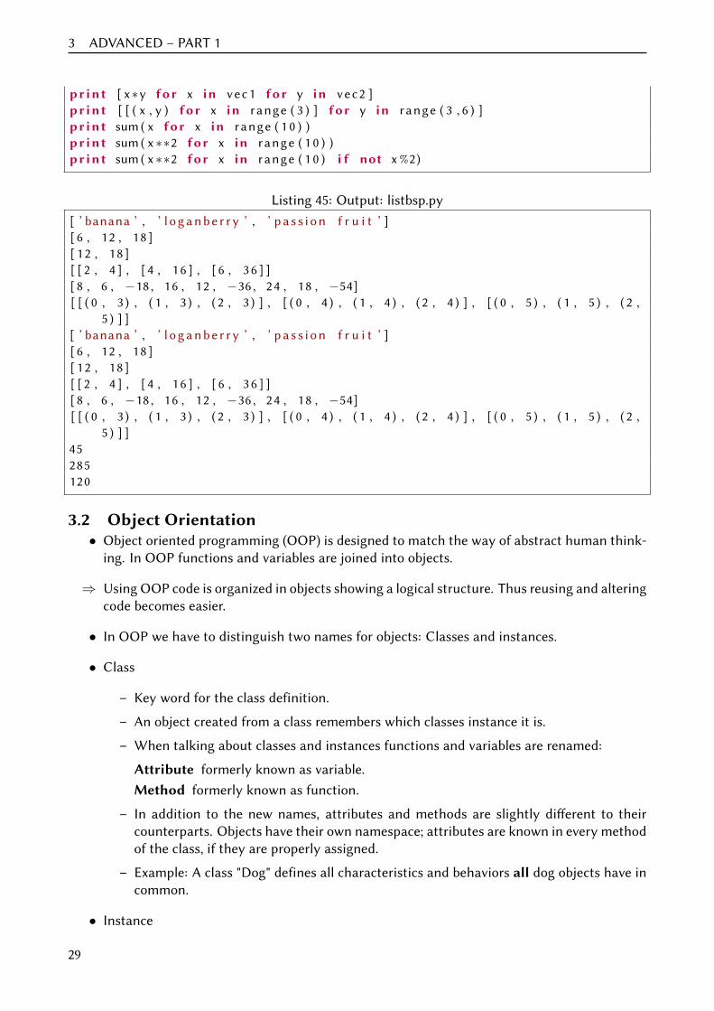
print [ x∗y for x in vec1 for y in vec2 ]print [ [ ( x , y ) for x in range ( 3 ) ] for y in range ( 3 , 6 ) ]print sum ( x for x in range ( 1 0 ) )print sum ( x ∗∗2 for x in range ( 1 0 ) )print sum ( x ∗∗2 for x in range ( 1 0 ) i f not x%2)

Listing 45: Output: listbsp.py[ ’ banana ’ , ’ l o g anbe r r y ’ , ’ p a s s i on f r u i t ’ ][ 6 , 1 2 , 18 ][ 1 2 , 18 ][ [ 2 , 4 ] , [ 4 , 1 6 ] , [ 6 , 3 6 ] ][ 8 , 6 , −18 , 16 , 1 2 , −36 , 2 4 , 1 8 , −54][ [ ( 0 , 3 ) , ( 1 , 3 ) , ( 2 , 3 ) ] , [ ( 0 , 4 ) , ( 1 , 4 ) , ( 2 , 4 ) ] , [ ( 0 , 5 ) , ( 1 , 5 ) , ( 2 ,

5 ) ] ][ ’ banana ’ , ’ l o g anbe r r y ’ , ’ p a s s i on f r u i t ’ ][ 6 , 1 2 , 18 ][ 1 2 , 18 ][ [ 2 , 4 ] , [ 4 , 1 6 ] , [ 6 , 3 6 ] ][ 8 , 6 , −18 , 16 , 1 2 , −36 , 2 4 , 1 8 , −54][ [ ( 0 , 3 ) , ( 1 , 3 ) , ( 2 , 3 ) ] , [ ( 0 , 4 ) , ( 1 , 4 ) , ( 2 , 4 ) ] , [ ( 0 , 5 ) , ( 1 , 5 ) , ( 2 ,

5 ) ] ]45285120

3.2 Object Orientation• Object oriented programming (OOP) is designed to match the way of abstract human think-ing. In OOP functions and variables are joined into objects.

⇒ Using OOP code is organized in objects showing a logical structure. Thus reusing and alteringcode becomes easier.

• In OOP we have to distinguish two names for objects: Classes and instances.

• Class

– Key word for the class deVnition.

– An object created from a class remembers which classes instance it is.

– When talking about classes and instances functions and variables are renamed:

Attribute formerly known as variable.Method formerly known as function.

– In addition to the new names, attributes and methods are slightly diUerent to theircounterparts. Objects have their own namespace; attributes are known in every methodof the class, if they are properly assigned.

– Example: A class "Dog" deVnes all characteristics and behaviors all dog objects have incommon.

• Instance

29

3 ADVANCED – PART 1

– An instance is the actual object created at run-time.

– Instances have

– The "Lassie" object is an instance of the Dog class.

Figure 1: Class and Instance

Listing 46: Example (Vrstclass.py)# ! / u s r / b i n / env python

c l a s s F i r s t C l a s s ( o b j e c t ) :a = " Foo "b = " Bar "

# No t i c e t h e key word " s e l f " !# Th i s i s most impo r t a n t f o r d e f i n i n g methods !def echo ( s e l f , x=None ) :

i f x :print x

e l se :print s e l f . a , s e l f . b

i f __name__== ’ __main__ ’ :c = F i r s t C l a s s ( )c . echo ( )

F i r s t C l a s s . a = 23c . echo ( )

Listing 47: Output: Vrstclass.py)Foo Bar23 Bar

• DeVning a class is similar to deVning a function. It expects an indented block.

• Methods in the class deVnition are simple functions, but in order to access the attributes ofthe class, the Vrst argument to a method has to be the object itself (usually called self). If itis missing, Python will issue an error stating that an unexpected number of arguments hasbeen passed to the method!

30

3 ADVANCED – PART 1

• The object self is just a reference on the instance. Using self you assure you are referencingthe instance itself.

• Notice: When calling a method of an instance the Vrst argument (self) is automaticallypassed to the method!

• If one writes e.g. FirstClass.a instead of self.a one is referencing the class with its valuesas given in the deVnition. Assigning FirstClass.a would change a in every instance!

• Properties of classes and instances

– Every method and attribute of a class or instance is also treated as an object.

– Instantiation of an object.

∗ Creating an instance is as simple as calling a function. In fact you can think of itas calling the objects __init__ method and passing arguments to that method.∗ The return value of calling a class is always an instance.

– Inheritance

∗ Each class can have a list of base classes from which it inherits methods and at-tributes.∗ Each inherited properties can be overwritten or expanded. In the latter case onerequires the function super() and the base classes to inherit from the object object.

⇒ When overwritting a method/attribute of a base class the overwritten property canbe referenced using super.

– Special methods and attributes

∗ Special names for methods (and attributes) have a greater meaning than just theirvalue or the code within them. Special attributes are set by the interpreter and arevery useful for condition tests.∗ For convenience all and only special names begin and end with two underscores!E.g. __init__().∗ Using special methods and attributes one can alter the principles of behavior ofobjects and overload operators like "+" or "*". As the most important and commonlyused can be considered these:

__init__() "Constructor"; this method is called upon creation of a new instance.__str__() This method is called when an object is passed to the print statement.__del__() "Destructor"; this method is called when the object is passed to the del statement.__add__() This method is called, when the object is added with something, e.g. inst1+inst2.

__bases__ Tuple of base classes.__name__ Name/type of class.

__class__ Class/type of instance.∗ For a full list of special names see Documentation.

Listing 48: Example (secondclass.py)# ! / u s r / b i n / env python

c l a s s F i r s t C l a s s ( o b j e c t ) :

31

3 ADVANCED – PART 1

a = " Foo "b = " Bar "

def echo ( s e l f , x=None ) :i f x :

print xe l se :

print s e l f . a , s e l f . b

c l a s s SecondClass ( F i r s t C l a s s ) :c = " He l l o World "

def _ _ i n i t _ _ ( s e l f , x=None ) :i f x :

s e l f . c = xprint s e l f . c

def _ _ s t r _ _ ( s e l f ) :return " I am SecondClass ! "

def echo ( s e l f , x=None ) :# c a l l i n g method echo ( ) o f t h e ba s e c l a s ssuper ( SecondClass , s e l f ) . echo ( )i f not x :

x = s e l f . cprint x

# __name__ i s a s p e c i a l a t t r i b u t e o f o b j e c t s# ( remember a l s o s c r i p t f i l e s a r e c o n s i d e r e d as o b j e c t s ! )i f __name__== ’ __main__ ’ :

# __name__ o f t h e i n i t i a l l y s t a r t e d s c r i p t i s " __main__ " .# t h e f o l l o w i n g l i n e s a r e on l y e x e c u t e d when t h i s f i l e i s# e x e c u t e d from th e command l i n e .s = SecondClass ( " Deutsch " )s . echo ( )

s . a , s . b = " Ha l l o " , " Welt "e = s . echoe ( )

print SecondClass , sSecondClass . echo ( s )

Notice: When calling a method of a class, one has to pass an instance object as Vrst argument tothe method!

Listing 49: Output: secondclass.pyDeutschFoo BarDeutschHa l l o WeltDeutsch

32

3 ADVANCED – PART 1

< c l a s s ’ __main__ . SecondClass ’ > I ’m SecondClass !Ha l l o WeltDeutsch

Listing 50: Example (thirdclass.py)# ! / u s r / b i n / env python

from s e c ond c l a s s import ∗

c l a s s Th i r dC l a s s ( SecondClass , F i r s t C l a s s ) :v a l u e1 = " Bla "v a l u e 2 = " Bla "

def _ _ i n i t _ _ ( s e l f , v1=None , v2=None ) :i f v1 : s e l f . v a l u e1 = v1i f v2 : s e l f . v a l u e 2 = v2

def echo ( s e l f ) :print s e l f . va lue1 , s e l f . v a l u e 2print "Which echo method i s t h i s ? "super ( Th i rdC la s s , s e l f ) . echo ( )

def s e t ( s e l f ,∗∗ arg ) :s e l f . v a l u e 1 = arg . ge t ( ’ v a l u e 1 ’ , s e l f . v a l u e 1 )s e l f . v a l u e 2 = arg . ge t ( ’ v a l u e 2 ’ , s e l f . v a l u e 2 )s e l f . echo ( )

i f __name__== ’ __main__ ’ :t = Th i r dC l a s s ( " Ha l l o " , " Welt " )t . echo ( )t . s e t ( v a l u e 1 = " Python " )

Notice

• ThirdClass has two base classes. Each of them has a method echo, but the interpreter isalways calling the Vrst method with that name that is found. Base classes are searchedrecursively from left to right (a base class of the Vrst base class is searched before the secondbase class, and so forth).

• Attributes of the form self.value1 used in methods are properties of the instance and are thuspreserved. Variables of the form v1 are only known within the method until the method hasVnished.

Listing 51: Output: thirdclass.pyHa l l o WeltWhich echo method i s t h i s ?Foo BarHe l l o WorldPython WeltWhich echo method i s t h i s ?Foo Bar

33

3 ADVANCED – PART 1

He l l o World

3.3 Modules – Writing & Documentation• As we have seen every Python script can be imported as a module. If you share your mod-ules/scripts with others you should give them some documentation.

• Python oUers us two methods of documenting our scripts:

– Comments are quite useful for explaining what a couple of lines are actually doing orwhy the problem has been solved in a certain way.

– For documenting whole modules (automatic generated documentation Vles, etc.) in aneasy way one can use "Docstrings".

• Docstrings are single-line or multiline strings. They are placed as the Vrst element in theindented block of classes, methods and functions.

• These Docstrings are used to generate the contents of the help statement. As we have seenthe help display shows the structure of the object upon which is was called and the Doc-strings within that structure.

Listing 52: Beispielmodul (module2bsp.py)# ! / u s r / b i n / env python

def func1 ( a , b ) :" " " Ha l l o Welt

D i e s e Funk t i o n g i b t Ha l l o Welt aus " " "pass

def func2 ( a= ’ Ha l l o ’ , b= ’ He l l o ’ ) :" " " Ha l l o Welt v . 2

E i n e neue V e r s i o n von Ha l l o Welt " " "

c l a s s h a l l o :" " " E i n e d o k umen t i e r t e K l a s s e

D i e s e Doku i s t t o t a l s i n n f r e i !E h r l i c h ! " " "def echo1 ( s e l f ) :

" " " Ke ine Funk t i o n " " "pass

def echo2 ( s e l f , t e s t ) :" " " D i e s e Fun k t i o n macht n i x " " "pass

t e s t 1 = ’ Te s t ’

34

3 ADVANCED – PART 1

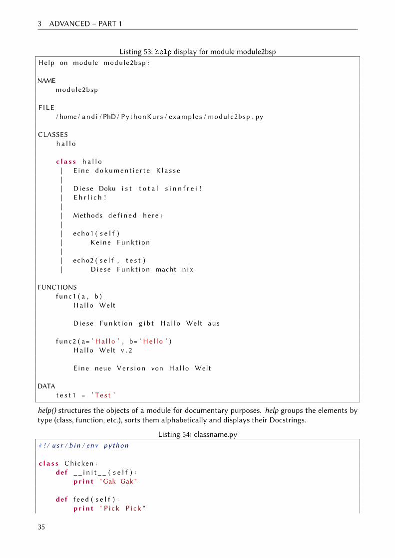
Listing 53: help display for module module2bspHelp on module module2bsp :

NAMEmodule2bsp

FILE/ home / and i /PhD/ PythonKurs / examples / module2bsp . py

CLASSESh a l l o

c l a s s h a l l o| E ine dokument i e r t e K l a s s e|| D iese Doku i s t t o t a l s i n n f r e i !| E h r l i c h !|| Methods de f i n ed here :|| echo1 ( s e l f )| Ke ine Funkt ion|| echo2 ( s e l f , t e s t )| D iese Funkt ion macht n i x

FUNCTIONSfunc1 ( a , b )

Ha l l o Welt

D iese Funkt ion g i b t Ha l l o Welt aus

func2 ( a= ’ Ha l l o ’ , b= ’ He l l o ’ )Ha l l o Welt v . 2

E ine neue Ve r s i on von Ha l l o Welt

DATAt e s t 1 = ’ Te s t ’

help() structures the objects of a module for documentary purposes. help groups the elements bytype (class, function, etc.), sorts them alphabetically and displays their Docstrings.

Listing 54: classname.py# ! / u s r / b i n / env python

c l a s s Chicken :def _ _ i n i t _ _ ( s e l f ) :

print "Gak Gak "

def f e ed ( s e l f ) :print " P i ck P i ck "

35

3 ADVANCED – PART 1

def l ay_egg ( s e l f ) :print " Egg "

print __name__c = Chicken ( )

Listing 55: classname2.py# ! / u s r / b i n / env python

c l a s s Chicken :def _ _ i n i t _ _ ( s e l f ) :

print "Gak Gak "

def f e ed ( s e l f ) :print " P i ck P i ck "

def l ay_egg ( s e l f ) :print " Egg "

i f __name__== ’ __main__ ’ :print __name__c = Chicken ( )

Listing 56: Output (classname.out)>>> import c lassname as nc lassnameGak Gak>>> print __name____main__

>>> import c las sname2 as m>>> m. Chicken ( )Gak Gak< c las sname2 . Chicken i n s t a n c e a t 0 x7 f254580ebd8 >

Notice: The code of scripts is executed upon import!

• The special attribute __name__ contains the name of the module.

• In the script passed to the interpreter for execution the value of __name__ is "__main__"⇔Its not an imported module, but themain script being run.

⇒ As we see in this example by testing __name__ we can deVne diUerent behaviors for scriptVles, e.g. opening a GUI, if its the main script, or not, if otherwise.

3.4 Exception Handling• Python – like other modern languages – oUers a comfortable and easy way of handling errors.

• Instead of writing code in order to prevent errors, one "catches" errors. This is known as"Exception Handling".

36

3 ADVANCED – PART 1

• Every error that can and will occur is an object, too!

⇒ Errors have properties, e.g. the attribute message.

• For the diUerent types of errors – e.g. wrong indentation, referencing unassined variable, etc.– the interpreter emits diUerent Exceptions.

Listing 57: Example>>> a = raw_input ( ’ I n t e g e r : ’ )I n t e g e r : 23>>> a+12Traceback ( most r e c e n t c a l l l a s t ) :

F i l e " < s td in > " , l i n e 1 , in <module >TypeEr ro r : cannot conca t ena t e ’ s t r ’ and ’ i n t ’ o b j e c t s

• The most common Exceptions are SyntaxError, TypeError and ValueError. For a full list anddescription see: Library Documentation.

• As all exception objects inherit from a BaseException class, we can even deVne our own ex-ceptions.

• Especially when writing modules it is quite handy to emit exceptions: e.g. raise KeyError,

'An error message' (see listing 60).

• To perform exception handling we need at least two statements: try and except.

Listing 58: Example>>> a = raw_input ( ’ I n t e g e r : ’ )I n t e g e r : 23>>> t ry :. . . a +12. . . except :. . . print " Geht n i c h t ! ". . .Geht n i c h t !

• The try statement introduces a block of code in which errors and exceptions can be handled.Execution will be stopped in the line where the error occured.

• The try block has to be followed by an except statement with a subsequent code block.

– The except statement can stand alone or with up to two arguments.

– The Vrst optional argument is an exception class, e.g. ValueError, or a sequence thereof.If this argument is given, the except block will only handle this particular exception.

– The second argument is a free variable name. The value of the message attribute willbe assigned to it.

⇒ A except statement without arguments will handle any exception.

⇒ After a try statement multiple except statements handling diUerent exceptions may occur.

37

3 ADVANCED – PART 1

⇒ If no except statement handles an exception ("unhandled exception") the script is terminatedas if the exception occured outside of a try block.

⇒ If an exception occurs within an except block it is also unhandled.

Listing 59: Example (exceptionbsp.py)# 1 / u s r / b i n / env python

while True :t ry :

t h e_ i npu t = raw_input ( ’ E ine Zahl : ’ )x = i n t ( t h e_ i npu t )break

except Va lueE r ro r , e r ro r_msg :print ’ Es t r a t e i n Problem auf : ’ , e r ro r_msg

except Keyboa rd In t e r rup t , e r ro r_msg :print ’ T schuess ’ , e r ro r_msgbreak

except EOFError , e r ro r_msg :print ’ Danke ’ , e r ro r_msgbreak

except :print ’ Es i s t e i n unvo rhe rge sehene r F eh l e r a u f g e t r e t e n ’print ’ B i t t e k on t a k t i e r e n S i e Ih r en Admin . . . ’break

• raise statement

– Instead of writing a piece of code containing a speciVc error, we can simple emit anexception using raise.

Listing 60: Example(raisebsp.out)>>> t ry :. . . ra i s e NameError , ’ Hi There ’. . . except NameError , e :. . . print ’An e x c ep t i o n f l ew by ’ , e. . . ra i s e. . .An e x c ep t i o n f l ew by Hi ThereTraceback ( most r e c e n t c a l l l a s t ) :

F i l e " < s td in > " , l i n e 2 , in <module >NameError : Hi There

– The raise statement expects an exception class and an optional string describing theerror.

– Even in older tutorials one often Vnds the variant "except Exception as e:". But upto version 2.5 this causes a SyntaxError!

– "Re-raise" – Calling raise within an except block will raise the exception handled by thisblock.

38

3 ADVANCED – PART 1

• else statement

– The else statement and a subsequent block are written after all except blocks.

– The else block is only executed, if the try block has been Vnished successfully.

⇒ Reduces code in the try block and hence the sources of exceptions in the try block.

Listing 61: Example (elseintry.py)# ! / u s r / b i n / env python

import sys

for arg in sys . a rgv [ 1 : ] :t ry :

f = open ( arg , ’ r ’ )except IOE r ro r :

print ’ cannot open ’ , a rge l se :

print arg , ’ has ’ , l e n ( f . r e a d l i n e s ( ) ) , ’ l i n e s ’f . c l o s e ( )

• We have already seen that exception handling allows us to perform actions on successfuland erroneous execution of the try block. Additionally we have the option to perform actionsindependent of the successful execution.

• Vnally statement

– The code block subsequent to the Vnally statement will be always executed.

– Even if an unhandled exception occurs, the Vnally block is executed, but the script willbe terminated thereafter.

– The Vnally block is executed, even if the try block has been ended using break, continueor return.

– Notice: return, break and continue can only occur within the try block, if the try blockis within a function, method or loop, respectively (see listing 59).

Listing 62: Example (Vnallybsp.py)# ! / u s r / b i n / env python

def d i v i d e 1 ( x , y ) :t ry :

r e s u l t = x / yexcept Ze r oD i v i s i o n E r r o r :

print " D i v i s i o n durch Nu l l . . . "e l se :

print " r e s u l t i s " , r e s u l tf i n a l l y :

print " e x e cu t i n g f i n a l l y c l a u s e "

def d i v i d e 2 ( x , y ) :

39

3 ADVANCED – PART 1

t ry :r e s u l t = x / y

except Ze r oD i v i s i o n E r r o r :print " D i v i s i o n durch Nu l l . . . "

except TypeEr ro r :print " Ungue l t i g e r Datentyp "print 1 / 0

e l se :print " r e s u l t i s " , r e s u l t

f i n a l l y :print " e x e cu t i n g f i n a l l y c l a u s e "

Listing 63: Example

>>> from f i n a l l y b s p import ∗>>> d i v i d e 1 ( 2 , 1 )r e s u l t i s 2e x e cu t i n g f i n a l l y c l a u s e>>> d i v i d e 1 ( 2 , 0 )D i v i s i o n durch Nu l l . . .e x e cu t i n g f i n a l l y c l a u s e>>> d i v i d e 1 ( ’ b ’ , ’ a ’ )e x e cu t i n g f i n a l l y c l a u s eTraceback ( most r e c e n t c a l l l a s t ) :

F i l e " < s td in > " , l i n e 1 , in <module >F i l e " f i n a l l y b s p . py " , l i n e 5 , in d i v i d e 1

r e s u l t = x / yTypeEr ro r : unsupported operand type ( s ) for / : ’ s t r ’ and ’ s t r ’>>> d i v i d e 2 ( 2 , 0 )D i v i s i o n durch Nu l l . . .e x e cu t i n g f i n a l l y c l a u s e>>> d i v i d e 2 ( 2 , ’ a ’ )Ungue l t i g e r Datentype x e cu t i n g f i n a l l y c l a u s eTraceback ( most r e c e n t c a l l l a s t ) :

F i l e " < s td in > " , l i n e 1 , in <module >F i l e " f i n a l l y b s p . py " , l i n e 20 , in d i v i d e 2

print 1 / 0Z e r oD i v i s i o n E r r o r : i n t e g e r d i v i s i o n or modulo by ze ro

• Module as deVned in listing 62 contains two functions for division.

• The function divide1 does not handle TypeErrors, e.g. string instead of a number.

• The function divide2 does handle TypeErrors, but contains a division by zero in this exceptblock: "1/0".

⇒ A ZeroDivisionError is emitted by divide2 each time a TypeError has initially occured.

⇒ The script will be terminated with an unhandled ZeroDivisionError.

40

4 ADVANCED – PART 2

4 Advanced – Part 24.1 Threading4.1.1 Threads• What is a thread?

– A thread is part of a program, that is executed independent from the rest.

⇒ The main program is a thread, too.

– Thread do not have to wait for other operations.

– On multi-core system threads can be executed simultaneously on diUerent cores.

– Threads are objects, too.

• Why threading?

– Only a threaded program can exhaust full capabilities of a modern computer system.

– Threads can run parallel and do not have to wait for each other.

– But there are limits to the parallelization caused by the hardware.

• threading module

– The class Thread provides everything needed for the thread.

⇒ To write a threaded program we need an object with base class Thread.

– The most important method of a thread is run; it is the "entry point" of the thread.

– For secure communication between threads: see Queue module.

Listing 64: Example (simplethread.py)# ! / u s r / b i n / env python

import cmathfrom t h r e ad i ng import Thread

c l a s s MyThread ( Thread ) :" Th i s i s our th read f o r do ing something . "

def run ( s e l f ) :" Th i s method i s c a l l e d when the th read i s s t a r t e d . "s e l f . d o _ s ome th i n g _pa r a l l e l ( )

def do_ s ome th i n g _pa r a l l e l ( s e l f ) :" Another method . We w i l l c a l l t h i s one l a t e r f o r pe r fo rming the

p a r a l l e l s t u f f . "while True :

( cmath . s i n ( 3 ) +cmath . cos ( 5 ) ) ∗cmath . tan ( 1 . 3 4 )

# i n s t a n t i a t i n g t h e o b j e c t .t = MyThread ( )# s t a r t i n g t h e t h r e a d .t . s t a r t ( )

41

4 ADVANCED – PART 2

# NOTICE : s t a r t ( ) has been c a l l e d , bu t i n t h e end run ( ) i s e x e c u t e d !

# What happens w i t h t h e t h r e a d when t h e main program has f i n i s h e d now?

Listing 65: Example (threadbsp.py)# ! / u s r / b i n / env python# −∗− c o d i n g : u t f −8 −∗−# t h r e a d b s p . py

import t h r e ad i ngimport time , da te t imeimport random

c l a s s MyThread ( t h r e ad i ng . Thread ) :"A more complex example o f how a thread can look l i k e . And now i t i s

a l s o doing something more "

def _ _ i n i t _ _ ( s e l f ) :" _ _ i n i t _ _ i s the s imp l e s t way o f pa s s i ng data to an o b j e c t "

# NOTICE : I f you w r i t e your own _ _ i n i t _ _# method , do no t f o r g e t t o c a l l t h e _ _ i n i t _ _# method o f t h e ba s e c l a s s !t h r e ad i ng . Thread . _ _ i n i t _ _ ( s e l f )

def run ( s e l f ) :" In t h i s method happens the ’ magic ’ "

s l e e p t ime = 1e−3 ∗ random . r and i n t ( 0 , 5000 )t ime . s l e e p ( s l e e p t ime )print date t ime . da te t ime . now ( ) . s t r f t i m e ( "%H:%M:%S .% f " ) , s t r ( s e l f )

# When work ing w i t h m u l t i p l e t h r e a d s s a v i n g them i n a l i s t i s q u i t ec om f o r t a b l e

j o b s = [ ]

for i in range ( 5 ) :j ob = MyThread ( )# Us ing t h e l i s t ’ s append method a new e l emen t i s appendedj o b s . append ( j ob )# Now we can s t a r t t h e t h r e a d .j ob . s t a r t ( )print date t ime . da te t ime . now ( ) . s t r f t i m e ( "%H:%M:%S .% f " ) , j ob

for j ob in j o b s :# As we have s e en i n s im p l e t h r e a d . py , t h e main# program was w a i t i n g f o r t h e t h r e a d . But t o be# on t h e s a v e s i d e we shou l d e x p l i c i t l y wa i t . . .j ob . j o i n ( )

Notice:

42

4 ADVANCED – PART 2

• The method __init__ of the base class has always to be called!

• When working with a large set of threads assigning them to list elements can be an elegantsolution.

• Even if the main program in listing 64 was waiting for threads to Vnish, this is no generalrule.

Listing 66: Output: threadbsp.py1 0 : 4 9 : 2 0 . 2 6 9 6 5 8 <MyThread ( Thread −1 , s t a r t e d 140087031699 2 00 ) >1 0 : 4 9 : 2 0 . 2 6 9 8 5 0 <MyThread ( Thread −2 , . . . ) >1 0 : 4 9 : 2 0 . 2 7 0 0 1 1 <MyThread ( Thread −3 , . . . ) >1 0 : 4 9 : 2 0 . 2 7 0 1 9 1 <MyThread ( Thread −4 , . . . ) >1 0 : 4 9 : 2 0 . 2 7 0 3 4 8 <MyThread ( Thread −5 , . . . ) >1 0 : 4 9 : 2 1 . 3 2 9 5 2 7 <MyThread ( Thread −5 , . . . ) >1 0 : 4 9 : 2 1 . 8 1 7 3 3 7 <MyThread ( Thread −1 , . . . ) >1 0 : 4 9 : 2 3 . 0 9 8 7 4 2 <MyThread ( Thread −2 , . . . ) >1 0 : 4 9 : 2 4 . 6 3 4 4 3 7 <MyThread ( Thread −3 , . . . ) >1 0 : 4 9 : 2 4 . 8 2 5 8 7 9 <MyThread ( Thread −4 , . . . ) >

• Remember:

– Use base class Thread.

– Don’t forget to call Thread.__init__() when overwritting __init__.

– Method run() is executed by the thread.

– Method start() starts the thread. If not called, the object is just a normal object.

– In order to wait for a thread call its join() method.

• The example of listing 65 could have been written shorter using another class from threading:Timer

Listing 67: Example (timerbsp.py)# ! / u s r / b i n / env python

import t h r e ad i ngimport random

def h a l l o ( i d ) :print " Ha l l o Welt . %s " % id

for i in range ( 1 0 ) :t = t h r e ad i ng . Timer ( random . r and i n t ( 0 , 1 0 ) , h a l l o , [ i , ] )t . s t a r t ( )

⇒ The Timer object runs a function after a given amount of time has passed. Passing of argu-ments to the function is also allowed.

• Python distinguishes between two types of threads:

43

4 ADVANCED – PART 2

– Daemon threads

– Non-daemon threads (default).

• There is no diUerence between those types except for: The entire Python program exitswhen no alive non-daemon threads are left.

4.1.2 Events & Locks

Listing 68: Example (threadbsp2.py)# ! / u s r / b i n / env python# −∗− c o d i n g : u t f −8 −∗−# t h r e a d b s p . py

import t h r e ad i ngimport t imeimport random

c l a s s MyThread ( t h r e ad i ng . Thread ) :

def run ( s e l f ) :s t ope r , i = random . r and i n t ( 1 0 0 , 1 0 0 0 ) , 0while True :

i += 1print s e l f . name , ’ says : ’ , ii f i > s t o p e r :

break

for i in range ( 1000 ) :MyThread ( ) . s t a r t ( )

• Notice Thread without a deVned __init__method as the initial method is inherited from thebase class.

• Each thread is writing to the display. As in many other cases the diUerent output strings aremixed up.

⇒ To avoid gibberish we need Events & Locks.

Listing 69: Output: threadbsp2.pyThread−207 says : 692Thread−207 says : 693Thread−207 says : 694

Thread−216 519 says : 602 Thread−212 says : says :5Thread −20194 Thread−217 says : says : says : 596

Thread −21322 Thread−212says : says : Thread−217Thread−210Thread−202 says : 60

44

4 ADVANCED – PART 2

says : 603says :

Thread−213 7 says :Thread −215757 Thread −21761

says : says : 5208

Thread −214440Thread−20195 Thread−216 409 Thread−206

Thread−199 says : says : 31 Thread−202Thread−212 says : Thread −215758604 says :

Thread−207 says : Thread−199 32 says :Thread−210 says : says : Thread −215759 says : 410 521695

The module threading oUers additionally to Thread objects a series of other objects for control-ling the behavior of threads. In the following we will have a closer look on Events and Locks.

• Event object

– Events manage one internal boolean attribute ("Flag"). Assignment and query of thisattribute are performed using methods of the event object.

– The initial value of this attribute after instantiation is False.

– Event objects have 4 important methods

set() Set the Wag to True.clear() Set the Wag to False.isSet() Return the Wag’s value.wait() The thread calling this method is waiting until the Wag becomes True. If the Wag is

already True when wait() is called, the call has no eUect.

– Events are designed to be global objects: any thread can set/clear them, all waitingthreads proceed when the Wag is True.

• Lock object

– Locks are like needle eyes. If multiple threads want to perform the same action at atime, locks ensure that maximal one thread can do so.

– Locks are designed to have two deVned states: locked and unlocked

– Like events the state of locks is switched using methods: acquire() & release()

– acquire()

∗ If unlocked, the state is changed to locked and the thread may proceed.∗ If locked, the thread has to wait until unlocked. Then one thread may proceedlike in the previous case.

– release()

∗ This method is only to be called when locked.∗ The state is set to unlocked.

45

4 ADVANCED – PART 2

– If multiple threads are waiting, acquire() and release() ensure that only one thread mayproceed.

• Both, lock and event objects themselves are referenced as usual. But one has to make surethat all threads see the same lock or event instance.

Listing 70: Example (threadbsp3.py)# ! / u s r / b i n / env python# −∗− c o d i n g : u t f −8 −∗−# t h r e a d b s p . py

import t h r e ad i ngimport t imeimport random

a l o ck = th r e ad i ng . Lock ( )

c l a s s MyThread ( t h r e ad i ng . Thread ) :

def run ( s e l f ) :s t ope r , i = random . r and i n t ( 1 0 0 , 1 0 0 0 ) , 0while True :

i += 1a l o ck . a c qu i r e ( )print s e l f . name , ’ says : ’ , ia l o c k . r e l e a s e ( )i f i > s t o p e r :

break

for i in range ( 1000 ) :MyThread ( ) . s t a r t ( )

• This example shows the code of listing 69 expanded by a lock object.

• In this case the lock object is an instance of the main thread; as such it is referenced fromwithin threads using the instance’s name; in this example alock.

• In most cases one would assign the lock instance to an attribute of a thread object. In thiscase referencing will become a bit more tricky as we will see in listing 75.

• Using the acquire and release method we have created a "needle eye": Only one thread at atime can write to the display.

Listing 71: Example (eventbsp.py)# ! / u s r / b i n / env python

import t h r e ad i ng as thimport random as r rimport t ime as t t

46

4 ADVANCED – PART 2

aevent = th . Event ( )

c l a s s EventWarter ( th . Thread ) :

def run ( s e l f ) :a even t . wa i t ( )t t . s l e e p ( r r . r a nd i n t ( 0 , 2100 ) ∗ 1e−3 )print s e l f

c l a s s Even tAu s l o s e r ( th . Thread ) :

def run ( s e l f ) :while True :

v a l u e = raw_input ( ’ En te r : ’ )i f va l u e == ’ even t ’ :

aeven t . s e t ( )break

for i in range ( 5 ) :EventWarter ( ) . s t a r t ( )

E v en tAu s l o s e r ( ) . s t a r t ( )

while th . a c t i v eCoun t ( ) > 1 :t t . s l e e p ( 2 e−1)

Listing 72: Output: eventbsp.pyEnte r : h a l l oEn te r : wor ldEn te r : e ven t< EventWarter ( Thread −5 , s t a r t e d 140069407471360 ) ><EventWarter ( Thread −3 , s t a r t e d 1400 694 2 4 2 5 6 768 ) ><EventWarter ( Thread −1 , s t a r t e d 14006944104 2 176 ) ><EventWarter ( Thread −4 , s t a r t e d 140069415864064 ) ><EventWarter ( Thread −2 , s t a r t e d 14 0069 43 2 6 4947 2 ) >

• The EventAusloser instance prompts for a string. If it is equal "event", the event is set and theloop aborted.

• Threads of type EventWarter wait for the event before they continue.

• Notice: If there were more threads interacting with I/O devices at the same time lock objectswould be required.

• Notice: The main program counts as a thread and threads are no longer active when codeexecution has Vnished.

Listing 73: Example (event2bsp.py)# ! / u s r / b i n / env python

47

4 ADVANCED – PART 2

import t h r e ad i ng as thimport t imeimport random

c l a s s Daemon ( th . Thread ) :mylock = th . Lock ( )

def run ( s e l f ) :while True :

# t h e e v e n t i s r e f e r e n c e d# u s i n g t h e c l a s s name !MyEvent . e ven t . wa i t ( )Daemon . mylock . a c qu i r e ( )print " Pong by " , s e l f . nameDaemon . mylock . r e l e a s e ( )

c l a s s MyEvent ( th . Thread ) :e ven t = th . Event ( )

def _ _ i n i t _ _ ( s e l f , l o op s ) :# a rgumen t s a r e pa s s e d t o t h e t h r e a d ;# t hu s we need an _ _ i n i t _ _ method .s e l f . l o op s = l oop s# do no t f o r g e t t o c a l l _ _ i n i t _ _ !th . Thread . _ _ i n i t _ _ ( s e l f )

def run ( s e l f ) :for l in range ( s e l f . l o op s ) :

t ime . s l e e p ( 1 e−3∗random . r and i n t ( 5 0 0 , 1 5 0 0 ) )print " P ing no . %d? " % lMyEvent . e ven t . s e t ( )MyEvent . e ven t . c l e a r ( )

for i in range ( 5 ) :t = Daemon ( )t . daemon = Truet . s t a r t ( )

m = MyEvent ( 3 )m. s t a r t ( )

Listing 74: Output: event2bsp.pyPing # 0?Pong by Thread−5Pong by Thread−1Pong by Thread−2Pong by Thread−3Pong by Thread−4Ping # 1?Pong by Thread−4Pong by Thread−5

48

4 ADVANCED – PART 2

Pong by Thread−1Pong by Thread−2Pong by Thread−3Ping # 2?

• The MyThread instance dominates the behavior of the script: it sets and clears an event.

• In response to those changes of the event threads of the type Daemon are printing a stringand their name to the command line.

⇒ As this output device is not "threadsafe" we need to use locks to prevent gibberish on thescreen.

⇒ Without the call of clear() the Daemon instances would not wait for the event, but work asfast as they could.

• Notice: As soon as theMyEvent thread has Vnished the main program will Vnish and termi-nate any active daemon thread: No response to "Ping no. 2?"

4.2 Queue• Queues oUer an elegant and threadsafe way of exchanging data between threads.

• Instead of starting a thread for each value one wants to process, one can start a couple ofthreads retrieving a value to process from the queue. This procedure is also more memory-friendly.

• The queue module provide three types of queues:

– Queue – a classical FIFO (First In First Out) queue. New elements are appended (put)at the end and retrieved (get) elements are taken from the beginning.

– LifoQueue – a classical LIFO (Last In First Out) Queue.

– Priority Queue (new in version 2.6)

• Queues can handle any type of data – including (function, class, etc.) instances.

• Values are passed to and from the queue using two methods of the queue instance:

put Appends an element to the queue.

get Retrieves an element of the queue.

• During instantiation of a queue one can deVne a maximum size of the queue.

• Depending on the queue conVguration these methods can raise exceptions, e.g. if the queueis empty or already full.

⇒ Queue speciVc exceptions: Empty and Full.

49

4 ADVANCED – PART 2

Listing 75: Example (queuebsp.py)

# ! / u s r / b i n / env python

from Queue import Queue , Emptyfrom t h r e ad i ng import Thread , Lock , a c t i v eCoun t

c l a s s Worker ( Thread ) :l o c k = Lock ( )

def run ( s e l f ) :while True :

t ry :i tem = q . ge t ( t imeout =5 )

except :break

Worker . l o c k . a c qu i r e ( )print " Es s ag t " , s e l f . name , ’ : ’ , i temWorker . l o c k . r e l e a s e ( )q . task_done ( ) # s i n c e v2 . 5 t h i s method# a c know l e g e s t h e s u c c e s s f u l t r e a tm e n t# o f t h e queue e l emen t .

q = Queue ( )for i in range ( 3 ) :

t = Worker ( )t . daemon = Truet . s t a r t ( )

for i in [ ’ Ha l l o ’ , ’ He l l o ’ , ’ S e r vus ’ , ’ Hi ’ , ’ Ahoi ’ ] :q . put ( i )

while ac t i v eCoun t ( ) >1 and not q . empty ( ) :pass

# s i n c e v2 . 5 t h i s method o r d e r s t h e c u r r e n t t h r e a d# t o wa i t f o r a l l queue e l emen t s t o be p r o c e s s e d .q . j o i n ( )

Listing 76: Output: queuebsp.py

Es s ag t Thread−1 : Ha l l oEs s ag t Thread−1 : He l l oEs s ag t Thread−1 : Se rvusEs s ag t Thread−1 : HiEs s ag t Thread−2 : Ahoi

Notice: If we had not used the methods task_done() and join() of the queue instance, there is aslight chance of the main program terminating before all queue elements are processed! Becausethe threads processing the data are daemon threads.

50

4 ADVANCED – PART 2

Listing 77: Beispiel (hw3.py)# ! / u s r / b i n / env python

import Tk i n t e r as T

r oo t = T . Tk ( )

l = T . Labe l ( root , t e x t = ’ Ha l l o Welt ! ’ )l . g r i d ( row = 0 , column = 0 )

q = T . Button ( root , t e x t = ’ Quit ’ , command= roo t . d e s t r oy )

q . g r i d ( row = 1 , column = 1 )

r o o t . mainloop ( )Figure 2: Screenshot

4.3 Graphical User Interfaces with Tk• Programs with graphical interfaces are nicer to look at and more Wexible and easier to usethan command line tools.

• Using Python we can choose from a variety of user interfaces:

– (n)curses / urwid (only available on Unix/Linux)

– Tk(inter) is a basic framework for writing GUIs on all platforms. It is part of the defaultinstallation on Windows systems. Some people consider Tk as "quick and dirty".

– GTK+ is a highly usable, feature rich toolkit. Its focus is on object orientation. It is oneof the major frameowrks used on Unix/Linux; on Windows libraries have to be installedseparately.

– Qt is another very powerful and popular toolkit for developing GUIs and command linetools, too. Like GTK+, libraries have to be installed separately on Windows systems.

– wxWidgets is an abstracted toolkit translating for generating GUIs using diUerent frame-works (e.g. Windows, GTK+, iPhone SDK, etc.).

• In this lecture we will focus on Tk.

• All neccessary objects for writing a GUI with Tk are provided by the module Tkinter.

• At Vrst one has to instantiate a Tk object. This object automatically creates a window (calledToplevel) which will contain any other elements to be displayed.

• This Tk instance has an important method called mainloop(). Before this method is callednothing will be displayed.

• In Tk and other GUI toolkits the elements of a window and the window itself are called"widgets".

• There is one important group of widgets with the ability to contain other widgets: containerwidgets, e.g. Frame, Toplevel

51

4 ADVANCED – PART 2

• To place widgets in those container widgets Tk provides two "geometry managers" – or inother words widgets have two methods for placing them into a container.

• Most widgets, especially container widgets, have a destroy method which makes the widgetdisappear. It is commonly used to destroy windows (Toplevel widgets).

• In Tk a variety of widgets is provided, but for the beginning we will have only a look on a fewreal important ones:

– Labels are simple widgets displaying text.

– Buttons are widgets a user can click on. If a Button is clicked, a callback function isexecuted (command argument in the widget instantiation).

• For further and more detailed information have a look into the documentation.

• In Tk we have two geometry managers:

– pack tries to place a widget on a side of the free space of the window.

– grid places the widgets on a table with cartesian coordinates.

• pack Geometry Manager

– Starting from an empty window with no extent the window is extended in a directioncontrary to the speciVed side in such a way that the widget can be placed on the speci-Ved side of the newly created free space.

– The pack method takes three arguments:

side side of free space on which the widget shall be placed (values: top, left, right,bottom).

Vll When more widgets are placed in a container they can hav diUerent extents result-ing in gaps (free space) in the container. Using this argument the widget can bestretched to Vll these gaps (values: x, y, both).

expand SpeciVes whether the widget is resized when the container is resized (values: 0, 1).anchor Further information on where to place a widget. It is a combination of the 4 direc-

tions (n, s, w, e).

• grid Geometry Manager

– Widget are placed into cells of a table by specifying the row and column of the cell.

– Empty rows and column are ignored (not displayed).

– Widget that are smaller than the speciVed space are centered. This can be overriddenusing the sticky option. sticky

– the grid method understands the following options:

row coordinate of the cell (count beginning at 0).column coordinate of the cell (count beginning at 0).sticky This options expects a string being a combination of the 4 directions (n, s, w, e), e.g.

’nw’.columnspan A widget can request multiple cells. This is the number of columns to use.

rowspan A widget can request multiple cells. This is the number of rows to use.

52

4 ADVANCED – PART 2

Listing 78: Example (tkpackbsp.py)# ! / u s r / b i n / env python

import Tk i n t e r as tk

def wind ( v ) :r o o t = tk . Tk ( )f rame1 = tk . Frame ( root , bg= ’ b lue ’ )f rame1 . pack ( s i d e = ’ top ’ , f i l l = ’ x ’ )l a b e l = tk . Labe l ( frame1 , t e x t = ’ Ha l l o

Welt ’ , r e l i e f = ’ g roove ’ )l a b e l . pack ( s i d e = ’ top ’ )f rame2 = tk . Frame ( root , bg= ’ ye l l ow ’ )f rame2 . pack ( s i d e = ’ l e f t ’ , f i l l = ’ both ’ ,

expand=v )l a b e l = tk . Labe l ( frame2 , t e x t = ’ Ha l l o

Welt ’ , r e l i e f = ’ g roove ’ )l a b e l . pack ( s i d e = ’ l e f t ’ )f rame3 = tk . Frame ( root , bg= ’ orange ’ )f rame3 . pack ( s i d e = ’ top ’ , f i l l = ’ both ’ )l a b e l = tk . Labe l ( frame3 , t e x t = ’ Ha l l o

Welt ’ , r e l i e f = ’ g roove ’ )l a b e l . pack ( s i d e = ’ top ’ )l a b e l = tk . Labe l ( frame3 , t e x t = ’ Ha l l o

Welt ’ , r e l i e f = ’ r i d g e ’ )l a b e l . pack ( s i d e = ’ l e f t ’ )r o o t . mainloop ( )

wind ( 0 )wind ( 1 )

(a) expand=0

(b) expand=1

Figure 3: Two windows afterresize. The frame with yel-low background color has beenpacked with diUerent expandvalues.

4.3.1 Geometry Manager – packIn order of the appearance in the source code:

• Blue frame: Placed at the top and set to Vll free space in x-direction.

• Yellow frame: Placed on the left side, Vlls in both directions. This frame behaves in thetwo windows diUerent!

• Orange frame: Placed on the top side of free space. As there is no free space above the blueframe it is placed below it. This frame also Vlls free space in both directions.

4.3.2 Geometry Manager – grid• Sticky value of the orange label is diUerent in the three examples.

• The widget is aligned towards the speciVed direction and/or stretched, if opposing directionsare speciVed.

Listing 79: Example: (tkgridbsp.py)

53

4 ADVANCED – PART 2

(a) sticky=’nw’ (b) sticky=’ns’ (c) sticky=’nswe’

Figure 4: grid example. Orange label has diUerent sticky values.

# ! / u s r / b i n / env python

import Tk i n t e r as tk

def wind ( s t i c k ) :r o o t = tk . Tk ( )for i in range ( 5 ) :

for j in range ( 6 ) :l a b e l = tk . Labe l ( root , t e x t = ’ (%d , %d ) ’ % ( i , j ) , r e l i e f = ’

r i d g e ’ )l a b e l . g r i d ( row= j , column= i )

l a b e l = tk . Labe l ( root , t e x t = ’ Mul t i ! ’ , bg= ’ ye l l ow ’ )l a b e l . g r i d ( row =2 , column =2 , columnspan =2 , rowspan =2 )l a b e l = tk . Labe l ( root , t e x t = ’ Ha l loWel t ’ , bg= ’ orange ’ )l a b e l . g r i d ( row =4 , column =1 , columnspan =2 , rowspan =2 , s t i c k y = s t i c k )r o o t . mainloop ( )

wind ( ’nw ’ )wind ( ’ ns ’ )wind ( ’ nswe ’ )

4.3.3 Widgets – Input• Text input

– By default one would use the Entry widget. It provides Veld of one line for user input.

– When a user is required to input more text one can use the Text widget which pro-vides multiple lines. If required or desired this widget can be made scrollable using theScrollbar widget.

– Notice: Working (programming) with Scrollbars in Tk is not intuitive, but it worksexactly as explained in the tutorial.

– Important methods of widgets for text input:

∗ get(): Read a string, that is currently displayed, from the widget.∗ insert(): Insert a string into the displayed string. Needs the position where toinsert.∗ delete(): Deletes displayed (sub-) string. Needs position where to delete.

• Widgets derived from the Button widget

54

4 ADVANCED – PART 2

– Radiobuttons can be grouped, e.g. like in multiple choice tests.

∗ Radiobuttons are grouped by assigning an IntVar instance to the variable option.∗ The value of the value option of the active Radiobutton is passed to the IntVarinstance.

– Checkbuttons can be turned on or oU. The current state of the button is saved in anIntVar instance, too.

– . . .

• Some other interesting widgets might be the Menu andMenubar widgets for creating menus.Quite helpful you can consider the Message widget, which is actually displaying "Popups".

Figure 5: A window containing several input widgets. Source: see listing 80.

Listing 80: Example (tkinput.py)# ! / u s r / b i n / env python

import Tk i n t e r as tkimport math

c l a s s Window :def _ _ i n i t _ _ ( s e l f ) :

s e l f . r o o t = tk . Tk ( )s e l f . r o o t . m in s i z e ( 1 5 0 , 1 0 0 )

s e l f . f rame = tk . Frame ( s e l f . r o o t )s e l f . f rame . pack ( s i d e = " top " , f i l l = " both " , expand =1 )

s e l f . e = tk . Ent ry ( s e l f . f rame )s e l f . e . pack ( s i d e = " top " , f i l l = " x " )

s e l f . c ho i c e = tk . I n tVa r ( )tk . Rad iobut ton ( s e l f . frame , t e x t = " s i n " , v a r i a b l e = s e l f . cho i ce , v a l u e

=1 ) . pack ( s i d e = " top " , anchor = "w" )tk . Rad iobut ton ( s e l f . frame , t e x t = " cos " , v a r i a b l e = s e l f . cho i ce , v a l u e

=2 ) . pack ( s i d e = " top " , anchor= "w" )

55

4 ADVANCED – PART 2

tk . Rad iobut ton ( s e l f . frame , t e x t = " tan " , v a r i a b l e = s e l f . cho i ce , v a l u e=3 ) . pack ( s i d e = " top " , anchor = "w" )

s e l f . op t i on = tk . I n tVa r ( )tk . Checkbutton ( s e l f . frame , t e x t = " R e s u l t i n mu l t i p l e s o f p i " ,

v a r i a b l e = s e l f . op t i on ) . pack ( s i d e = ’ top ’ , anchor = "w" )

tk . Button ( s e l f . frame , t e x t = " Ca l c u l a t e " , command= s e l f . c a l c ) . pack (s i d e = " top " , f i l l = " x " )

s e l f . e r g e bn i s = tk . Labe l ( s e l f . f rame )s e l f . e r g e bn i s . pack ( s i d e = " top " , f i l l = " x " )

tk . Button ( s e l f . frame , t e x t = " Quit " , command= s e l f . r o o t . q u i t ) . pack (s i d e = " top " , f i l l = " both " , expand =1 )

s e l f . r o o t . mainloop ( )

def c a l c ( s e l f ) :t ry :

wert = f l o a t ( s e l f . e . ge t ( ) )f unk t i on = s e l f . c ho i c e . ge t ( )

except :pass

e l se :i f f unk t i on ==1 :

wert = math . s i n ( wert )e l i f f unk t i on ==2 :

wert = math . cos ( wert )e l i f f unk t i on ==3 :

wert = math . tan ( wert )

i f s e l f . op t i on . ge t ( ) :wert = s t r ( wert / math . p i ) + ’ p i ’

s e l f . e r g e bn i s . c o n f i g u r e ( t e x t = s t r ( wert ) )

w = Window ( )

• In listing 80 the Tk application has been embedded in a separate class. We can consider thisas a step forward, but when things get a bit more complicated one has to be careful.

⇒ When writing code one should ensure that is elegant. In this context it means, one shouldseparate code for the GUI from code doing something else, e.g. calculations, etc.

• Good programming style is considered to be

– Write an object-oriented program designed for the command line.

– Afterwards write a GUI (so-called frontend).

• As we see in the listing IntVar objects do not behave like simple integers. The IntVar classprovides two methods for setting (set()) and getting (get()) the value inside of it.

56

4 ADVANCED – PART 2

4.3.4 Events• Events in Tk are bit diUerent than in threading. Events are not set by the script, but by theuser interacting with the program. So, we have a set of deVned events available:

– Pressing a button on the keyboard.

– Pressing a button on the mouse.

– Moving the mouse into a widget or out of it.

• In the threading module we were waiting for events, now we are binding widgets and eventsto a function or method using the bind method of a widget: widget.bind(event, callback).

• In the call of the bind method the event is described as a string with a given syntax:

– Each event is identiVed by a string of the type: <modifier-type-detail>.

type The important part specifying the type of the event, e.g. (mouse) button click.

detail Detailed optional information, e.g. which mouse button.

modiVer Optional addition, e.g. "double" click.

• Some commonly used events:

– <Button-n> – Mouse click, n = 1 left, n = 2 middle, n = 3 right

– <Bn-Motion> – Mouse movement while button pressed.

– <Double-Button-n> – Mouse double click; also modiVer Triple possible.

– <Enter>/<Leave> – Mouse enters/leaves widget.

– <Key> – The well-known "any key" key has been pressed.

– <Shift-Up> – Key combination "Shift" and "Arrow Up"; detail may be any other direc-tion, too.

– <Configure> – Window has been resized.

– Full list of events see Events.

• Event objects in Tk have attributes specifying where the event happend:

– widget – widget instance, in which the event happend.

– x,y – Relative position of mouse at that moment.

– x_root,y_root – Absolute position of mouse on screen at that time.

– width,height – Size of the widget. If it is a resize event, this is the new size.

– type – Integer representing the type of the event.

• For more details see Intro. to Tkinter.

Listing 81: Example (inputtkbsp.py)# ! / u s r / b i n / env pythonimport Tk i n t e r as tkimport math as mm

c l a s s window :

57

4 ADVANCED – PART 2

def _ _ i n i t _ _ ( s e l f ) :s e l f . f = tk . Tk ( className= " Ca l c u l a t o r " )l = tk . Labe l ( s e l f . f , t e x t = ’ Berechnung : ’ , r e l i e f = ’ r i d g e ’ )l . g r i d ( row = 0 , column = 0 , s t i c k y = ’we ’ )s e l f . e= tk . Ent ry ( s e l f . f , width = 10 )s e l f . e . g r i d ( row = 1 , column = 0 , s t i c k y = ’we ’ )b1 = tk . Button ( s e l f . f , t e x t = ’ s i n ( x ) ’ , command = s e l f . s i n )b1 . g r i d ( row = 2 , column = 0 , s t i c k y = ’we ’ )b2 = tk . Labe l ( s e l f . f , t e x t = ’ cos ( x ) ’ , r e l i e f = ’ r a i s e d ’ )# NOTICE : I n t h e b ind c a l l t h e c a l l b a c k method# s e l f . c o s has no p a r e n t h e s e s ! ! !b2 . b ind ( ’ <Button−1> ’ , s e l f . cos )b2 . g r i d ( row = 3 , column = 0 , s t i c k y = ’we ’ )s e l f . e r g e bn i s = tk . Labe l ( s e l f . f , r e l i e f = ’ r i d g e ’ )s e l f . e r g e bn i s . g r i d ( row =4 , column =0 , s t i c k y = ’we ’ )

s e l f . f . mainloop ( )

def s i n ( s e l f ) :s e l f . out (mm. s i n ( f l o a t ( s e l f . e . ge t ( ) ) ) )

def cos ( s e l f , e ven t ) :s e l f . out (mm. cos ( f l o a t ( s e l f . e . ge t ( ) ) ) )print even t . widget , e ven t . x , e ven t . y

def out ( s e l f , w) :s e l f . e r g e bn i s . c o n f i g u r e ( t e x t = s t r (w) )

w = window ( )

• Notice: The callback methods for button "b1" and label "b2" are written without parantheses.

• We do not want the methods to be executed when the button is instantiated or the eventbound to the label.

⇒ Therefore the arguments are function/method objects.

• To callback functions/methods an event instance is passed automatically.

• The programmer has no inWuence on how the Tk mainloop is calling callback methods.

⇒ No other data can be passed to the callback method.

⇒ If more data is needed, it has to be retrieved from attributes or by calling other methods.

• A Button object does not need to be bound to a button event, it has a shortcut: the optioncommand binds the button to a callback. The buttons callback function receives no argumentsunless its a method of an object. In that case it only receives an instance reference (self).

• The callback bound to an Event receives one more argument than in the previous case: anEvent object.

58

4 ADVANCED – PART 2

Figure 6: Screenshot (inputtkbsp.py)

Figure 7: Screenshot (tkevent.py)

• Labels are bound to the entering (<Enter>) and leaving (<Leave>) of the mouse.

• Notice: In the method deVnition the instance self is written before the event instance.

• The widget attribute of the event is an actual reference to the widget. This way we couldmanipulate that widget.

Listing 82: (tkevent.py)# ! / u s r / b i n / env python

import Tk i n t e r as tk

c l a s s Window :

def echo1 ( s e l f , e ven t ) :s e l f . l a b e l 2 . c o n f i g ( t e x t = "Mouse en t e r ed the widget \ n%s " % event .

widget )

def echo2 ( s e l f , e ven t ) :s e l f . l a b e l 2 . c o n f i g ( t e x t = "Mouse l e f t the widget \ n%s " % event .

widget )

def _ _ i n i t _ _ ( s e l f ) :s e l f . r o o t = tk . Tk ( )

s e l f . f rame = tk . Frame ( s e l f . r o o t )s e l f . f rame . pack ( s i d e = " top " , f i l l = " both " )

s e l f . l a b e l 0 = tk . Labe l ( s e l f . frame , t e x t = " He l l o World " , r e l i e f = "r i d g e " )

s e l f . l a b e l 0 . pack ( s i d e = " top " , f i l l = " both " , expand =1 )

59

4 ADVANCED – PART 2

s e l f . l a b e l 1 = tk . Labe l ( s e l f . frame , t e x t = " Ha l l o Welt " , r e l i e f = "groove " )

s e l f . l a b e l 1 . pack ( s i d e = " top " , f i l l = " both " , expand =1 )

s e l f . l a b e l 2 = tk . Labe l ( s e l f . frame , t e x t = " " )s e l f . l a b e l 2 . pack ( s i d e = " bottom " , expand =0 )

s e l f . l a b e l 0 . b ind ( ’ < Enter > ’ , s e l f . echo1 )s e l f . l a b e l 0 . b ind ( ’ <Leave > ’ , s e l f . echo2 )s e l f . l a b e l 1 . b ind ( ’ < Enter > ’ , s e l f . echo1 )s e l f . l a b e l 1 . b ind ( ’ <Leave > ’ , s e l f . echo2 )s e l f . r o o t . mainloop ( )

Window ( )

60

5 MODULES FOR SCIENCE

5 Modules for science• In Python is a series of "high-performance" modules for scientiVc purposes available. Thesemodules are Python code wrapped around compiled C++ or Fortran programs.

• NumPy is the most important module for numerical calculations.

– Provides additional data types and performant mathematical operations.

– The list of Velds of mathematics covered by NumPy is long, but some interesting Veldsmight be:

∗ Functions adapted for handling the new data types.∗ Financial math∗ Linear algebra∗ Fouriertransformation∗ and more

– This module also provides tools for implementing or wrapping of Fortran, C & C++code.

• SciPy is an "extension" module for NumPy.

– Imports NumPy on its own as it needs support for arrays.

– For better performance allmost all functions are written in Fortran.

– Math capabilites expanded by:

∗ Integration & Derivation∗ Optimization∗ Rare mathematical functions and physical constants.

• Matplotlib or Pylab does the visualization.

– 2D plotting library for publication quality Vgures.

– Rich set of examples and screenshots.

– The plotting commands are fully customizable (e.g. line width, color and style, etc.)

– This module is not limited to plotting. Displayed Vgures can be turned to interactiveinterfaces with dragable objects (e.g. for background removal of a spectrum).

– The module matplotlib.pyplot containing the most important elements for plotting hasa shortcut: pylab

– pylab imports NumPy automatically as it needs support for arrays, too.

• A very good source for examples and ideas: Cookbook for NumPy & SciPy.

• Due to our limited time we can have just a quick look on some of the most important basicsof the scientiVc modules:

numpy New data types.

numpy How NumPy’s mathematical functions aUect these new data types.

scipy Integrals and Derivatives in (NumPy and) SciPy.

61

5 MODULES FOR SCIENCE

scipy Special functions of SciPy. A quick look on where to Vnd them.

pylab Simple 2D plots with legends and labelling of axes.

• These topics we will not talk about:

– "Most of the stuU".

– Programming in C and Fortran.

– Wrapping C and Fortran programs.

– Complex capabilites of the matplotlib module.

Figure 8: Some examples.

5.1 NumPy5.1.1 Arrays• A new data type intruduced by NumPy is the Array. It is very similar to Python’s lists, but itis behaving diUerently sometimes, e.g. under summation.

• Creating an array is straight forward. We can create on from a sequence of values or use oneof NumPy’s easy to use functions:

– array(sequence,dtype,...) – Transforms a sequence into an array.

62

5 MODULES FOR SCIENCE

– ones(shape,dtype) – shape is a sequence deVning the dimension and size of the array,which will be Vlled with ones. Passing dtype to the function one can set the data typeof the array elements.

– zeros(...) – As ones, but all values are zero.

– empty(...) – As ones, but values are read from "debris" in the system memory.

– arange(start,stop,stepsize,dtype) – As range, but stepsize does not have to be an integer.

– linspace(start,stop,steps,...). As arange, but steps deVnes the length of the array.

– logspace(...) As linspace, but using a logarithmic scale.

Listing 83: Example (num0bsp.out)>>> import numpy as n>>> # Umwandlung L i s t e i n Ar ray. . . a = n . a r r ay ( [ 1 , 2 , 5 , 6 , 7 , 9 , 2 3 , 4 2 ] )>>> # Da ten typ von a ?. . . a . dtypedtype ( ’ i n t 6 4 ’ )b = n . ones ( ( 3 , 3 ) )>>> ba r r ay ( [ [ 1 . , 1 . , 1 . ] ,

[ 1 . , 1 . , 1 . ] ,[ 1 . , 1 . , 1 . ] ] )

>>> # t h e upper l i m i t 3 w i l l NEVER be p a r t o f t h e a r r a y. . . # t h e d i f f e r e n c e be tween n e i g h b o r i n g e l emen t s i s t h e s t e p s i z e 0 . 2 5. . . n . a range ( 1 , 3 , . 2 5 )a r r ay ( [ 1 . , 1 . 2 5 , 1 . 5 , 1 . 7 5 , 2 . , 2 . 2 5 , 2 . 5 , 2 . 7 5 ] )>>> # empty ( ) doe s no t a s s i g n v a l u e s t o t h e e l emen t s .. . . # Whatever i s i n t h e memory i s used as v a l u e .. . . n . empty ( ( 2 , 2 ) )a r r ay ( [ [ 6 . 9 3 8 1 8 2 5 5 e−310 , 9 . 9 8 2 4 5 8 0 4 e−317] ,

[ 8 . 7 6 4 9 4 1 9 5 e−317 , 8 . 7 6 4 9 3 0 0 9 e−317 ] ] )>>> # t h e upper l i m i t I S p a r t o f t h e a r r a y .. . . # No t i c e t h e l o g ( ) f u n c t i o n s i n t h e l o g s p a c e c a l l .. . . n . l o g spa c e ( n . l o g ( 1 ) , n . l o g ( 3 ) , 5 , base =n . exp ( 1 ) )a r r ay ( [ 1 . , 1 . 3 1 6 0 7 4 0 1 , 1 . 7 3 2 0 5 0 8 1 , 2 . 2 7 9 5 0 7 0 6 , 3 . ] )

• As we have seen earlier Python determines data types automatically. But in the case ofarrays, we can override this mechanism and choose a data type for array elements:

– Default numerical data types, e.g. int, float.

– C-style data types, e.g. int64, uint64.

• When we think about vectors in linear algebra these vectors behave diUerently than Python’ssequences. Arrays in NumPy are very similar to those vectors:

– Addition of Python lists returns one concatenated list.

– Multiplication of a Python list is only deVned with an integer resulting in multipleconcatenations.

63

5 MODULES FOR SCIENCE

– Arrays can be added and multiplied with any scalar (int, Woat, ...) or another array ofthe same size.

⇒ Any mathematical operation on an array is performed on each element.

– Except for mathematics arrays behave like lists.

Listing 84: Example (num1bsp.out)>>> import numpy as n>>> # 1−dim . A r r ay s. . . a , b = n . a r r ay ( ( 1 , 2 , 3 ) , ’ complex ’ ) , n . l i n s p a c e ( 0 , 2 , 3 )>>> a , b( a r r ay ( [ 1 . + 0 . j , 2 . + 0 . j , 3 . + 0 . j ] ) , a r r ay ( [ 0 . , 1 . , 2 . ] ) )>>> # No t i c e t h e d i f f e r e n c e i n add ing a r r a y s and l i s t s !. . . a . r e a l +b , [ 1 , 3 , 5 ] + [ 0 , 1 , 2 ]( a r r ay ( [ 1 . , 3 . , 5 . ] ) , [ 1 , 3 , 5 , 0 , 1 , 2 ] )>>> # Adding a s c a l a r. . . a +3.5−2 ja r r ay ( [ 4 . 5 −2 . j , 5 . 5 −2 . j , 6 . 5 −2 . j ] )>>> # S c a l a r p r o du c t>>> n . i nn e r ( a , b )( 8+0 j )>>> # D e f i n i n g 2−d imen s i o n a l a r r a y s. . . d = n . a r r ay ( [ [ 2 , 3 , 4 ] , [ 3 , 4 , 5 ] , [ 7 , 8 , 9 ] ] , dtype= ’ f l o a t ’ )>>> # Ca s t i n g t h e da t a t yp e o f a r r a y e l emen t s>>> a=a . a s type ( ’ f l o a t ’ )>>> # E x c e p t f o r math , a r r a y s behave j u s t l i k e l i s t s , . e . g e l emen t

a s s i g nmen t .>>> a [ 1 ]= n . p i>>> aa r r ay ( [ 1 . 0 0 0 0 0 0 0 0 + 0 . j , 3 . 1 4 1 5 9 2 6 5 + 0 . j , 3 . 0 0 0 0 0 0 0 0 + 0 . j ] )

Listing 85: Examples (num2bsp.out)>>> # l e t ’ s go t o t h e t h i r d d imen s i on. . . c = n . random . random ( ( 2 , 2 , 2 ) )>>> ca r r ay ( [ [ [ 0 . 3 2 3 4 1 3 5 9 , 0 . 8 8 4 9 7 7 3 1 ] ,

[ 0 . 1 5 2 3 6 9 7 2 , 0 . 9 4 5 2 0 9 2 9 ] ] ,

[ [ 0 . 2 2 3 0 2 6 5 1 , 0 . 8 2 8 3 6 4 1 8 ] ,[ 0 . 8 6 7 7 7 1 2 2 , 0 . 3 2 6 6 4 0 2 6 ] ] ] )

>>> # we can i n c r e a s e t h e s i z e i n one d imen s i on by r e p e a t i n g e l emen t s. . . t =c . r e p e a t ( 2 , 2 )>>> ta r r ay ( [ [ [ 0 . 3 2 3 4 1 3 5 9 , 0 . 3 2 3 4 1 3 5 9 , 0 . 8 8 4 9 7 7 3 1 , 0 . 8 8 4 9 7 7 3 1 ] ,

[ 0 . 1 5 2 3 6 9 7 2 , 0 . 1 5 2 3 6 9 7 2 , 0 . 9 4 5 2 0 9 2 9 , 0 . 9 4 5 2 0 9 2 9 ] ] ,

[ [ 0 . 2 2 3 0 2 6 5 1 , 0 . 2 2 3 0 2 6 5 1 , 0 . 8 2 8 3 6 4 1 8 , 0 . 8 2 8 3 6 4 1 8 ] ,[ 0 . 8 6 7 7 7 1 2 2 , 0 . 8 6 7 7 7 1 2 2 , 0 . 3 2 6 6 4 0 2 6 , 0 . 3 2 6 6 4 0 2 6 ] ] ] )

>>> # Ano the r e x c e p t i o n : S l i c e s o f a r r a y s can be d e f i n e s u s i n g t h i s :. . . t [ : , : : − 1 , 2 ]

64

5 MODULES FOR SCIENCE

a r r ay ( [ [ 0 . 9 4 5 2 0 9 2 9 , 0 . 8 8 4 9 7 7 3 1 ] ,[ 0 . 3 2 6 6 4 0 2 6 , 0 . 8 2 8 3 6 4 1 8 ] ] )

>>> # D e f i n i n g p i e c e w i s e f u n c t i o n s i s a common t a s k .. . . n . p i e c ew i s e ( t , [ t > . 5 , t < = 0 . 5 ] , [ True , F a l s e ] )a r r ay ( [ [ [ 0 . , 0 . , 1 . , 1 . ] ,

[ 0 . , 0 . , 1 . , 1 . ] ] ,

[ [ 0 . , 0 . , 1 . , 1 . ] ,[ 1 . , 1 . , 0 . , 0 . ] ] ] )

>>> # Th i s won ’ t work : c : ( 2 , 2 , 2 ) , d : ( 2 , 2 , 4 ). . . c+ tT raceback ( most r e c e n t c a l l l a s t ) :

F i l e " < s td in > " , l i n e 1 , in <module >Va l u eE r r o r : shape mismatch : o b j e c t s cannot be b r oadca s t to a s i n g l e shape

Notice:

• Referencing subarrays of arrays can be done as known from other sequences. Additionallyone can use just one pair of square brackets and separate the indeces by comma.

• The numpy module oUers a series of mathematical functions and operators (e.g. sin() orinner(). Furthermode functions for manipulating arrays (e.g. repeat() or select()) are provided,too.

⇒ see NumPy Doc: Functions by Category.

• Some operators and functions (e.g. outer()) expecting at least two arrays as arguments canwork with arrays of diUerent size, but the vast majority will produce a "ValueError: shapemismatch".

Listing 86: Examples (num3bsp.out)>>> import numpy as n>>> import numpy . random as nr>>> a = n . ones ( [ 4 , 4 ] , dtype=n . f l o a t 9 6 )>>> a # j u s t a 2D a r r a ya r r ay ( [ [ 1 . 0 , 1 . 0 , 1 . 0 , 1 . 0 ] ,

[ 1 . 0 , 1 . 0 , 1 . 0 , 1 . 0 ] ,[ 1 . 0 , 1 . 0 , 1 . 0 , 1 . 0 ] ,[ 1 . 0 , 1 . 0 , 1 . 0 , 1 . 0 ] ] , dtype= f l o a t 9 6 )

>>> # b and c a r e q u i t e s i m i l a r e x c e p t f o r t h e . copy ( ). . . b , c = a [1 : −1 , 1 : −1 ] , a [ 1 : −1 , 1 : −1 ] . copy ( )>>> ba r r ay ( [ [ 1 . 0 , 1 . 0 ] ,

[ 1 . 0 , 1 . 0 ] ] , dtype= f l o a t 9 6 )>>> # Each e l emen t o f b and c i s changed .. . . b [ : ] , c [ : ] = . 5 ∗ n . pi , n . p i>>> b , c( a r r ay ( [ [ 1 . 5 7 0 7 9 6 3 , 1 . 5 7 0 7 9 6 3 ] ,

[ 1 . 5 7 0 7 9 6 3 , 1 . 5 7 0 7 9 6 3 ] ] , dtype= f l o a t 9 6 ) , a r r ay ( [ [ 3 . 1 4 1 5 9 2 7 ,3 . 1 4 1 5 9 2 7 ] ,

[ 3 . 1 4 1 5 9 2 7 , 3 . 1 4 1 5 9 2 7 ] ] , dtype= f l o a t 9 6 ) )>>> a # No t i c e t h e d i f f e r e n c e i n a !

65

5 MODULES FOR SCIENCE

a r r ay ( [ [ 1 . 0 , 1 . 0 , 1 . 0 , 1 . 0 ] ,[ 1 . 0 , 1 . 5 7 0 7 9 6 3 , 1 . 5 7 0 7 9 6 3 , 1 . 0 ] ,[ 1 . 0 , 1 . 5 7 0 7 9 6 3 , 1 . 5 7 0 7 9 6 3 , 1 . 0 ] ,[ 1 . 0 , 1 . 0 , 1 . 0 , 1 . 0 ] ] , dtype= f l o a t 9 6 )

>>> a = [ [ 1 for x in range ( 3 ) ] for y in range ( 3 ) ]>>> a # a good o l d f r i e n d , a l i s t c omprehen s i on[ [ 1 , 1 , 1 ] , [ 1 , 1 , 1 ] , [ 1 , 1 , 1 ] ]>>> b = a [ 1 ] [ 1 ]>>> b1>>> b = 3>>> a # No t i c e t h e d i f f e r e n c e i n b e h a v i o r t o a r r a y s ![ [ 1 , 1 , 1 ] , [ 1 , 1 , 1 ] , [ 1 , 1 , 1 ] ]>>> c=nr . rand ( 2 , 2 )>>> c . f l a t t e n ( )a r r ay ( [ 0 . 0 0 1 0 2 9 7 5 , 0 . 2 7 2 2 3 2 5 , 0 . 2 7 7 2 2 8 4 8 , 0 . 7 1 1 7 8 1 2 6 ] )>>> # Some q u i t e impo r t a n t methods o f a r r a y s. . . c . max ( ) , c . argmax ( )( 0 . 7 1 1 7 8 1 2 6 1 9 4 3 5 1 7 3 2 , 3 )>>> n . r o t 9 0 ( c )a r r ay ( [ [ 0 . 2 7 2 2 3 2 5 , 0 . 7 1 1 7 8 1 2 6 ] ,

[ 0 . 0 0 1 0 2 9 7 5 , 0 . 2 7 7 2 2 8 4 8 ] ] )

Notice:

• Referencing all elements of an array can be done with b[:], not just with b[:,:,...].

• Subarrays behave diUerently than subsets of sequences. Subarrays are considered to be"links" or pointers to the actual array. Changing a value in a subarray aUects the valuein the original array, too!

⇒ To get an independent subarray from an array one has to use the method copy().

• Remember: Listing 86 shows the most dangerous trap in numpy after using the wrong datatype:

– The assignment b=a does not create a new array b, it only provides a link to parts of theoriginal array a.

– This behavior is similar for the other data types introduced with NumPy. As we haveseen in listing 86 assigning subsets of normal lists to a new variable is truely an assign-ment.

– To create a new array use copy(). Thus the new array is independent from the originalone.

• Among the functions, methods and operators provided by NumPy we have seen so far youmight be intereted in some of these in order to solve problems:

– Watten() and ravel() transform an N dimensional array into a one dimensional one.

– reshape() is more general than Watten(), the result does not have to be 1 dimensional.But the size or number of elements within the array can not be altered.

– append(): You know that one from lists.

66

5 MODULES FOR SCIENCE

– concatenate() joins a sequence of arrays and returns one big array. Arrays must havethe same number of dimensions.

– rot90(), Wipud(), Wiplr(): Returns a rotated od Wipped copy of the array.

– argmin(), argmax(), min(), max(): Finding extrema in an array is a commonly performedtask. These methods return the value of the position of the extremum.

• In the previous example we have encountered a submodule for generating random numbers.But numpy.random oUers more, e.g.:beta(), poisson(), binomial(), rand(), randint(), randn()

5.1.2 Masked Arrays• A very useful modiVcation of the array type is themasked array from the submodule numpy.ma.

• Masked arrays contain additionaly to their data a mask of the same shape.

• NumPy and modules depending on it ignore data in masked elements. Useful for

– Handling polar data in cartesian array.

– Masking bogus data in experimental measurements.

– Blanking singularities.

• How to mask?

– By explicitly creating a masked array from a data and mask array with the functionmasked_array.

– By explicitly assigning single array elements the special value numpy.ma.masked.

– By using one of the other predeVned functions.

• DeVnition similar to normal array except for an additional argument.

• The mask array speciVes where the data shall be not accessible.

1 means element in masked.

0 means element is not masked.

Listing 87: Example (maskedarrays.py)# ! / u s r / b i n / env python# −∗− c o d i n g : u t f 8 −∗−

import numpyimport numpy .maimport py lab

x = numpy . arange ( 0 , 1 0 , . 1 )y = numpy . o n e s _ l i k e ( x )z = y . copy ( )z [ 4 0 : 6 0 ] = numpy . nany [ 4 0 : 6 0 ] = 2

67

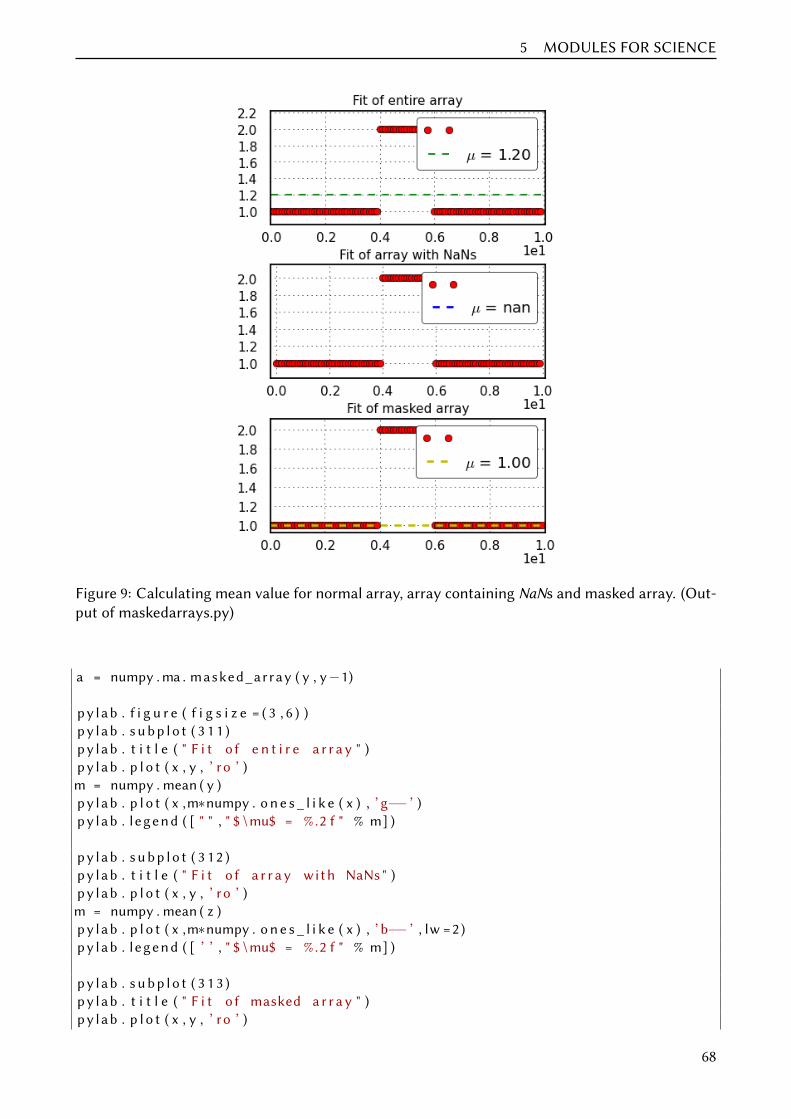
5 MODULES FOR SCIENCE

Figure 9: Calculating mean value for normal array, array containing NaNs and masked array. (Out-put of maskedarrays.py)

a = numpy .ma . masked_array ( y , y−1)

py lab . f i g u r e ( f i g s i z e = ( 3 , 6 ) )py lab . s ubp l o t ( 3 1 1 )py lab . t i t l e ( " F i t o f e n t i r e a r r ay " )py lab . p l o t ( x , y , ’ ro ’ )m = numpy . mean ( y )py lab . p l o t ( x ,m∗numpy . o n e s _ l i k e ( x ) , ’ g−− ’ )py lab . l egend ( [ " " , " $ \mu$ = %.2 f " % m] )

py lab . s ubp l o t ( 3 1 2 )py lab . t i t l e ( " F i t o f a r r ay with NaNs " )py lab . p l o t ( x , y , ’ ro ’ )m = numpy . mean ( z )py lab . p l o t ( x ,m∗numpy . o n e s _ l i k e ( x ) , ’ b−− ’ , lw =2 )py lab . l egend ( [ ’ ’ , " $ \mu$ = %.2 f " % m] )

py lab . s ubp l o t ( 3 1 3 )py lab . t i t l e ( " F i t o f masked a r r ay " )py lab . p l o t ( x , y , ’ ro ’ )

68

5 MODULES FOR SCIENCE

m = numpy . mean ( a )py lab . p l o t ( x ,m∗numpy . o n e s _ l i k e ( x ) , ’ y−− ’ , lw =2 )py lab . l egend ( [ ’ ’ , " $ \mu$ = %.2 f " % m] )

py lab . show ( )

Listing 88: Example (maskedarrays.out)>>> import numpy , numpy .ma>>> a = numpy . a r r ay ( ( 1 , 4 , 2 , 4 , 2 , 4 , 3 5 , 2 , 9 9 ) )>>> aa r r ay ( [ 1 , 4 , 2 , 4 , 2 , 4 , 3 5 , 2 , 9 9 ] )>>> a . mean ( )1 7 . 0>>> a [−3]=numpy .ma . masked>>> a [−1]=numpy .ma . masked>>> aa r r ay ( [ 1 , 4 , 2 , 4 , 2 , 4 , 0 , 2 , 0 ] )>>> # Masking an o r d i n a r y a r r a y doe s no t work. . . a . mean ( )2 . 1 1 1 1 1 1 1 1 1 1 1 1 1 1 1 2>>> a = numpy .ma . a r r ay ( ( 1 , 4 , 2 , 4 , 2 , 4 , 3 5 , 2 , 9 9 ) )>>> amasked_array ( data = [ 1 4 2 4 2 4 35 2 9 9 ] ,

mask = Fa l s e ,f i l l _ v a l u e = 999999 )

>>> a [−1]=numpy .ma . masked>>> a [−3]=numpy .ma . masked>>> amasked_array ( data = [1 4 2 4 2 4 −− 2 −−],

mask = [ F a l s e F a l s e F a l s e F a l s e F a l s e F a l s e True F a l s eTrue ] ,

f i l l _ v a l u e = 999999 )>>> a . mean ( )2 . 7 1 4 2 8 5 7 1 4 2 8 5 7 1 4 4>>> a . compressed ( )a r r ay ( [ 1 , 4 , 2 , 4 , 2 , 4 , 2 ] )>>> a . compressed ( ) . mean ( )2 . 7 1 4 2 8 5 7 1 4 2 8 5 7 1 4 4

• Arrays from module numpy cannot be masked. One needs arrays from the module numpy.mato support masking!

• numpy.ma also contains a function array(), but which creates a masked array, where the maskis set to False (or 0) everywhere.

• By assigning numpy.ma.masked to an array element, the element gets masked.

– In the data represented by two dashes “- -”.

– In the mask indicated by the value True.

69

5 MODULES FOR SCIENCE

• The method compressed() of masked arrays returns an ordinary array with the unmaskeddata.

• A quick overview of further functions for the creation of masked arrays

Vx_invalid() Return input with invalid data masked and replaced by a Vll value.

masked_greater() Mask an array where greater than a given value (also masked_less andmasked_greater_equal).

masked_where Mask an array where a condition is met.

• For full list see Constructing masked arrays.

• One can mask an entire array by setting the mask attribute to True.

• There are two kinds of masks.

hard mask a masked element is truely not accessible.

soft mask default, when assigning a new value to a masked element it becomes unmasked. Toapply a soft mask one has to

∗ call the soften_mask method of the array or∗ apply the keyword argument hard_mask=False during array creation.

Listing 89: Example (maskedimage.py)# ! / u s r / b i n / env python

import Imageimport numpyimport numpy .maimport s c i p y . op t im i z eimport py labimport ma t p l o t l i b . cm

y = numpy . l oad ( " data . npy " )data = numpy . s q r t ( ( y [ 0 , : , : ] − y [ 2 , : , : ] ) ∗∗2 + ( y [ 1 , : , : ] − y [ 3 , : , : ] ) ∗∗2 )data2 = data / data . max ( ) ∗ 255

im = Image . f romar ray ( data2 . a s type ( " u i n t 8 " ) , " L " )im . save ( " mask_2D_preedi t . png " )

# Now you shou l d have e d i t e d t h e image w i t h GIMP and# s a v ed your mask as ’ ma sk_2D_po s t e d i t . png ’ .

maskim = Image . open ( " mask_2D_posted i t . png " )mask = numpy . a r r ay ( maskim . ge tda t a ( ) ) . r e shape ( ( 1 0 2 4 , 1 0 2 4 ) )da ta2 = numpy .ma . masked_array ( data , mask )

# Now you go t a masked a r r a y w i t h ou t any d i s t u r b i n g# e l emen t s f o r f u r t h e r t r e a tm e n t .

py lab . f i g u r e ( f i g s i z e = ( 1 2 , 6 ) )

70

5 MODULES FOR SCIENCE

py lab . s ubp l o t ( 1 2 1 )py lab . imshow ( data , cmap=ma t p l o t l i b . cm . s p e c t r a l )py lab . c o l o r b a r ( o r i e n t a t i o n = " h o r i z o n t a l " )

py lab . s ubp l o t ( 1 2 2 )py lab . imshow ( data2 , cmap=ma t p l o t l i b . cm . s p e c t r a l )py lab . c o l o r b a r ( o r i e n t a t i o n = " h o r i z o n t a l " )

py lab . show ( )

Figure 10: Unmasked and masked array.

• Numpy oUers the functions save and load to save/load arrays to/from Vles.

• The contents of the Vle data.npy in this example contains experimental data.

• For more complex masks one can export arrays as images.

– The Python Imaging Ligrary oUers everything for the handling of image Vles.

– The image data has to be in the range [0, 1] or [0, 255].

– External manipulation of the mask image.

• The manipulated “binary” mask image is transformed back to an array. Don’t forget to adjustthe shape of the array.

5.1.3 Matrices• The data type matrix has inherited lots of its properties from arrays.

• As we have seen, arrays are equivalent to vectors in mathematics, but matrices are reallymatrices in a mathematical sense.

⇒ From this analogy to mathematical structures we can derive properties for the data type ofmatrices and point out the diUerences to arrays:

– Matrices are always two-dimensional.

71

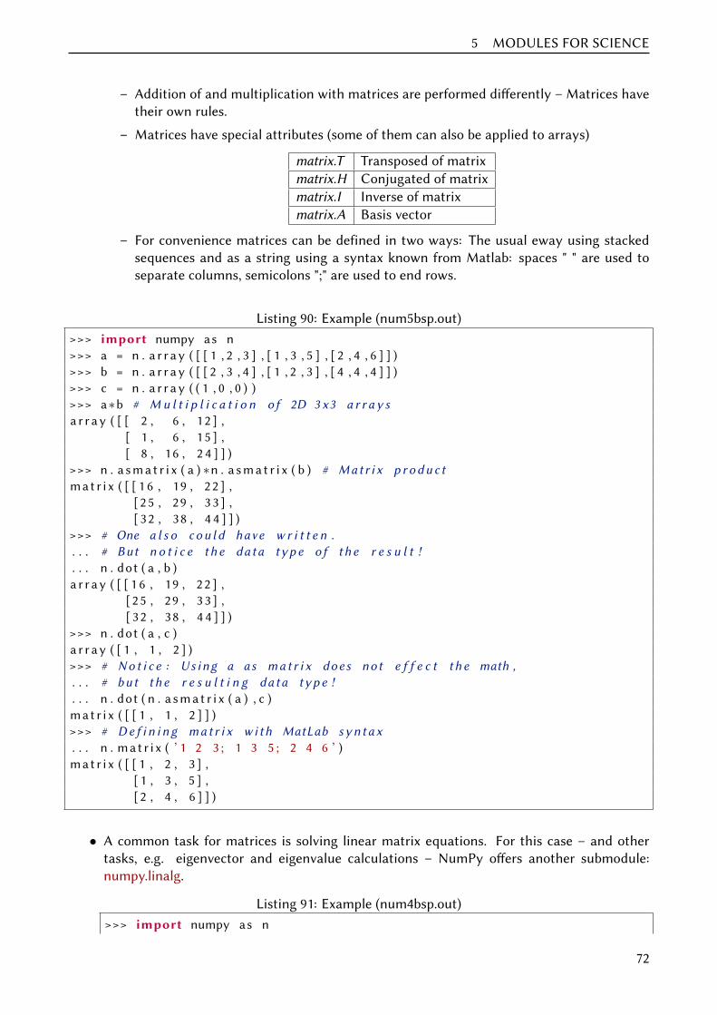
5 MODULES FOR SCIENCE

– Addition of and multiplication with matrices are performed diUerently – Matrices havetheir own rules.

– Matrices have special attributes (some of them can also be applied to arrays)

matrix.T Transposed of matrixmatrix.H Conjugated of matrixmatrix.I Inverse of matrixmatrix.A Basis vector

– For convenience matrices can be deVned in two ways: The usual eway using stackedsequences and as a string using a syntax known from Matlab: spaces " " are used toseparate columns, semicolons ";" are used to end rows.

Listing 90: Example (num5bsp.out)>>> import numpy as n>>> a = n . a r r ay ( [ [ 1 , 2 , 3 ] , [ 1 , 3 , 5 ] , [ 2 , 4 , 6 ] ] )>>> b = n . a r r ay ( [ [ 2 , 3 , 4 ] , [ 1 , 2 , 3 ] , [ 4 , 4 , 4 ] ] )>>> c = n . a r r ay ( ( 1 , 0 , 0 ) )>>> a∗b # M u l t i p l i c a t i o n o f 2D 3 x3 a r r a y sa r r ay ( [ [ 2 , 6 , 1 2 ] ,

[ 1 , 6 , 1 5 ] ,[ 8 , 1 6 , 2 4 ] ] )

>>> n . a sma t r i x ( a ) ∗n . a sma t r i x ( b ) # Ma t r i x p r o du c tmat r i x ( [ [ 1 6 , 1 9 , 2 2 ] ,

[ 2 5 , 2 9 , 3 3 ] ,[ 3 2 , 3 8 , 4 4 ] ] )

>>> # One a l s o c ou l d have w r i t t e n .. . . # But n o t i c e t h e da t a t yp e o f t h e r e s u l t !. . . n . dot ( a , b )a r r ay ( [ [ 1 6 , 1 9 , 2 2 ] ,

[ 2 5 , 2 9 , 3 3 ] ,[ 3 2 , 3 8 , 4 4 ] ] )

>>> n . dot ( a , c )a r r ay ( [ 1 , 1 , 2 ] )>>> # No t i c e : Us ing a as ma t r i x doe s no t e f f e c t t h e math ,. . . # bu t t h e r e s u l t i n g da t a t yp e !. . . n . dot ( n . a sma t r i x ( a ) , c )mat r i x ( [ [ 1 , 1 , 2 ] ] )>>> # D e f i n i n g ma t r i x w i t h MatLab s y n t a x. . . n . ma t r i x ( ’ 1 2 3 ; 1 3 5 ; 2 4 6 ’ )mat r i x ( [ [ 1 , 2 , 3 ] ,

[ 1 , 3 , 5 ] ,[ 2 , 4 , 6 ] ] )

• A common task for matrices is solving linear matrix equations. For this case – and othertasks, e.g. eigenvector and eigenvalue calculations – NumPy oUers another submodule:numpy.linalg.

Listing 91: Example (num4bsp.out)>>> import numpy as n

72

5 MODULES FOR SCIENCE

>>> import numpy . l i n a l g as l

>>> # a t r i v i a l example on s o l v i n g. . . # l i n e a r ma t r i x e q u a t i o n s. . . >>> a = n . mat r i x ( [ [ 1 , 2 ] , [ − 4 , 5 ] ] )>>> v = n . a r r ay ( [ 4 , − 7 ] )>>> a , v( mat r i x ( [ [ 1 , 2 ] ,

[−4 , 5 ] ] ) , a r r ay ( [ 4 , −7]) )>>> # How c o n f e n i e n t , t h e f u n c t i o n t o. . . # s o l v e t h e e q u a t i o n i s c a l l e d. . . x = l . s o l v e ( a , v )>>> # a n a l y t i c a l r e s u l t : [ 3 4 / 1 3 , 9 / 1 3 ] .. . . # And c h e c k i n g whe the r t h e r e s u l t i s c o r r e c t. . . x , n . dot ( a , x ) , va r r ay ( [ 2 . 6 1 5 3 8 4 6 2 , 0 . 6 9 2 3 0 7 6 9 ] ) , ( ma t r i x ( [ [ 4 . , −7 . ] ] ) , a r r ay ( [ 4 ,−7]) )

• Caution: As the name NumPy suggests, all data and calculations based on this module arepurely numerical.

⇒ Even if an equation is known to have no solution, the numerical function solve() will return aresult. Therefore one has to check results for their plausibility.

Listing 92: Example (num6bsp.out)

>>> import numpy as n>>> import numpy . l i n a l g as l

>>> a = n . mat r i x ( [ [ 1 , 2 , 3 ] , [ 4 , 5 , 6 ] , [ 7 , 8 , 9 ] ] )>>> b = n . a r r ay ( [ 4 , − 5 , 1 3 ] )>>> c= l . s o l v e ( a , b )>>> print c , ’ \ nThese v e c t o r s a re NOT equa l : \ n ’ , n . dot ( a , c ) , ’ ! = ’ , b[ 6 . 0 7 8 3 7 5 5 2 e +16 −1 .21567510 e +17 6 . 0 7 8 3 7 5 5 2 e +16]These v e c t o r s a r e NOT equa l :[ [ 1 6 . 1 6 . 1 6 . ] ] ! = [ 4 −5 13 ]

5.1.4 Polynomials• Polynomials are known in Numpy as the poly1d data type.

• With this data type a minimum of symbolic math is available to NumPy. The symbolicmath capabilites are restricted to the most commonly used operations like integration andderivation. See NumPy Reference Manual on Polynomials.

• Polynomials can be thought of as arrays containing the coeXcients of the polynomial. As apolynomial is considered a function in mathematics they have to behave so in NumPy, too.

• DeVning a polynomial is done straight forward using poly1d( with a sequence of coeXcients.Alternatively, one can use a confenience function poly() which accepts a sequence of roots ofthe polynomial.

73

5 MODULES FOR SCIENCE

• As already mentioned, symbolic math is limited to basic arithmetics, integration and deriva-tion. For each of these operations a special function is provided.

• Finally, a well known Vtting mechanism is also provided: polyVt(x,y,deg) Vts a Taylor seriesin the range x to the data (or function) y.

Listing 93: Example (polybsp.py)# ! / u s r / b i n / env python

import py lab as p# py l ab a u t om a t i c a l l y impo r t s numpy t o t h e s c r i p t

# c o o r d i n a t e r angex = p . arange ( −2 . 5 , 2 . 5 , . 0 1 )X = p . arange (−1 .5∗p . pi , 1 . 5 ∗ p . pi , . 0 1 )

y0 = p . po ly1d ( [ 4 , 0 , 1 ] )y1 = p . po l yde r ( y0 , 1 )y2 = p . po l yde r ( y0 , 2 ) # e qua l t o p o l y d e r ( y1 , 1 )

# N o t i c e : p o l y f i t r e t u r s a l i s t o f c o e f f i c i e n t s ,# bu t no po l ynom ia l !f 1 = p . po ly1d ( p . p o l y f i t ( X , p . s i n ( X ) ∗∗ 2 , 5 ) )f 2 = p . po ly1d ( p . p o l y f i t ( X , p . s i n ( X ) ∗∗ 2 , 8 ) )

# About p l o t t i n g we w i l l t a l k l a t e r ;− )p . s ubp l o t ( 2 1 1 )# D e r i v a t i v e s o f p o l y n om i a l sp0 = p . p l o t ( x , y0 ( x ) , ’ r ’ , x , y1 ( x ) , ’ g ’ , x , y2 ( x ) , ’ b ’ )p . l egend ( p0 , [ " $y$ " , " $dy / dx$ " , " $d ^2y / dx ^2 $ " ] , 0 )p . g r i d ( )

p . s u bp l o t ( 2 1 2 )# Tay l o r s e r i e sp1 = p . p l o t ( X , p . s i n ( X ) ∗∗2 , ’ r ’ , X , f 1 ( X ) , ’ g ’ , X , f 2 ( X ) , ’ b ’ )p . l egend ( p1 , ( ’ $ s i n ^2 ( x ) $ ’ , ’O$x^5$ ’ , ’O$x^8$ ’ ) , 0 )p . g r i d ( )

p . show ( )

Additionally we will now take a look on an actually reasonable example where we are usingpolynomials and a function from the numpy module: select()

Listing 94: (polywurfbsp.py)# ! / u s r / b i n / env python

import py lab as p

t = p . arange ( 0 , 6 , . 0 1 )# i n i t i a l v e l o c i t y andd h e i g h tv0 = 15

74

5 MODULES FOR SCIENCE

Figure 11: Output: polybsp.py

h0 = 60

a = p . po ly1d ( [ − 9 . 8 1 , ] )v = p . p o l y i n t ( a , 1 , v0 )h = p . p o l y i n t ( v , 1 , h0 )

p . p l o t ( t , a ( t ) , lw =2 )p . p l o t ( t , p . s e l e c t ( [ h ( t ) >0 ,h ( t ) < 0 ] , [ v ( t ) , 0 ] ) , lw =2 )p . p l o t ( t , p . s e l e c t ( [ h ( t ) >0 ,h ( t ) < 0 ] , [ h ( t ) , 0 ] ) , lw =2 )p . l egend ( [ ’ A c c e l e r a t i o n ’ , ’ V e l o c i t y ’ , ’ Height ’ ] )p . g r i d ( )p . show ( )

Notice how the values of height and velocity are set to zero and remain zero as the object hitsthe ground.

5.2 SciPy• NumPy oUers a lot of functionality. But there are some things missing, e.g. we had no toolsfor numerical integration.

75

5 MODULES FOR SCIENCE

Figure 12: Output: trajectory parabola (polywurfbsp.py)

• This "gap" is another module (based on Fortran) Vlling: SciPy. SciPy extends the set of toolsoUered by NumPy or replaced parts from it, e.g. bot modules have submodules for Fouriertransformations.

• For now we will take only a view on some selected features of SciPy. To discover SciPy inmore detail see SciPy Reference Manual.

• Physical and mathematical constants (since version 0.7.0!)

– Provided by submodule scipy.constants.

– The submodule returns the value or unit of a constant when calling the correspondingfunction value() or unit(). Both functions expect a string with the constant’s name. Seea full list of constant names.

– The most common and important constants can be called using a shortcut of the formscipy.constants.constant, e.g. scipy.constants.g or scipy.constants.zero_Celsius.

– Alternatively one can use the module physcon, which is the predecessor of the SciPysubmodule.

• Fourier transformation

– Provided by scipy.Utpack which is a more feature-rich alternative to numpy.Utpack. Itcan be used for these purposes:

∗ Fast Fourier Transforms

76

5 MODULES FOR SCIENCE

∗ DiUerential and pseudo-diUerential operators∗ Convolutions

• Special functions – or from special Velds of science – which are not very common are "out-sourced" to an extra submodule.

– The submodule scipy.special covers among others these Velds:

∗ Airy Functions∗ Elliptic Functions and Integrals∗ Bessel Functions (Integrals & Derivatives)∗ Gamma and Related Functions∗ etc.

• For computating integrals SciPy provides a separate submodule called scipy.integrate.

5.2.1 Derivation• The module scipy.Utpack provides tools for derivations, Fourier transformations and convo-lutions.

• In most cases diU() is a good choice.

• This function calculates derivatives of data sets. Unlike derivatives of polynomials the diU()operator works only on arrays containing data.

• The diU() operator takes up to three arguments

– The sample which is to derive.

– The order of derivations (default: 1).

– The periodicity of the sample (default: 2π).

Listing 95: Example (scipyderivbsp.py)# ! / u s r / b i n / env python

import py lab as pimport s c i p y . f f t p a c k as s f

x = p . arange (−3∗p . pi , 3∗p . pi , . 0 0 1 )y = lambda x : p . s i n ( x )

yy1 = s f . d i f f ( y ( x ) , o rde r =1 , p e r i od =2∗p . p i )yy2 = s f . d i f f ( y ( x ) , o rde r =1 , p e r i od =4∗p . p i )yy3 = s f . d i f f ( y ( x ) , o rde r =1 , p e r i od =6∗p . p i )

p l = p . p l o t ( x , y ( x ) , x , yy1 , x , yy2 , x , yy3 )p . l egend ( pl , [ " $y = \ s i n ( x ) $ " , " $dy / dx ( 2 \ p i ) $ " , " $dy / dx ( 4 \ p i ) $ " , " $dy / dx ( 6 \

p i ) $ " ] , 0 )p . g r i d ( )p . x l a b e l ( ’ x ’ )p . y l a b e l ( ’ y ’ )p . show ( )

77

5 MODULES FOR SCIENCE

Figure 13: Output of scipyderivbsp.py. Derivatives of the sine function for diUerent periodicities.

• In listing 95 the calculated derivatives can be quite faulty like the solutions of linear matrixequations. Except here we can tune the diU() operator.

⇒ To get a good result one should choose the sample size to be a multiple of the periodicity (inthe mathematical sense) of the function or data set.

⇒ The periodicity argument for the diU() operator should be the length of the sample.

• In the example of listing 95 the periodicity of the sine function equals 2π and we had chosena x-range of 6π. For the diU() operator the correct periodicity is 6π.

Listing 96: Example (scipyderiv2bsp.py)# ! / u s r / b i n / env python

import py lab as pimport s c i p y . f f t p a c k as s f

x = p . arange (−3∗p . pi , 3∗p . pi , . 0 0 1 )y = p . exp (−x ∗∗2 )yy = s f . d i f f ( y , o rde r =1 , p e r i od =6∗p . p i )Y = s f . d i f f ( y , o rde r =−1 , p e r i od =6∗p . p i )p l = p . p l o t ( x , y , x , yy , x , Y )p . l egend ( pl , [ " $y=e^{−x ^ 2 } $ " , " $dy / dx$ " , " $ \ i n t \ , y \ , dx$ " ] , 0 )p . g r i d ( )p . show ( )

• If we want to diUerentiate a function with diU(), the function does not have to be periodic ina mathematical sense as you can see in listing 96.

78

5 MODULES FOR SCIENCE

Figure 14: Gaussian curve with derivative and integral (as calculated by diff).

• The sample that shall be diUerentiated has to be periodic. In listing 96 the Gaussian curve iscentered on the sample. Thus contatenating the sample periodicaly results in a sample thatlooks periodic. And thus a non-periodic function can be diUerentiated.

• Notice: In examples with functions that are equal or near to zero at the sample boundariesthere are no oscillations in the derivative. In the other cases those oscillations can be smalleUects on the margin or dominate the whole sample.

⇒ Concatenating has to result in a continuous sample.

• In order to diUerentiate a non-periodic and/or discontinuous function the sample has to beexpanded such that the original sample is part of a periodic and continuous bigger sample.

Listing 97: Example (scipyderiv3bsp.py)# ! / u s r / b i n / env python

import py lab as pimport s c i p y . f f t p a c k as s f

x = p . arange (−2∗p . pi , 2 ∗ p . pi , . 0 1 )y = p . cos ( x )z = p . a r c t an ( x )

X = p . arange (−2∗p . pi , 6 ∗ p . pi , . 0 1 )Z = p . conca t ena t e ( ( z , z [ : : − 1 ] ) )Z −= Z [ 0 ]

yy = s f . d i f f ( y , p e r i od =4∗p . p i )z z = s f . d i f f ( z , p e r i od =4∗p . p i )

79

5 MODULES FOR SCIENCE

Figure 15: Derivatives of (top) a periodic function and (bottom) a non-periodic function that is not contin-uous either. See listing 97

ZZ = s f . d i f f ( Z , p e r i od =8∗p . p i )

p . f i g u r e ( )p . s u bp l o t ( 2 1 1 )p l 1 = p . p l o t ( x , y , x , yy )p . l egend ( p l1 , [ " $y = \ cos ( x ) $ " , " $dy / dx$ " ] , 0 )p . g r i d ( )

p . s u bp l o t ( 2 1 2 )p l 2 = p . p l o t ( x , z , x , z z )p . l egend ( p l2 , [ " $z = \mathrm { a r c t an } ( x ) $ " , " $dz / dx$ " ] , 0 )p . g r i d ( )

p . f i g u r e ( )p l 3 = p . p l o t ( X / p . p i , Z , X / p . p i , ZZ )p . l egend ( p l3 , [ " $z = \mathrm { a r c t an } ( x ) $ i n $ [−2\ pi , 2 \ p i ] $ " , " $dz / dx$ " ] , 0 )p . x l a b e l ( " $x / \ p i $ " )p . g r i d ( )p . show ( )

5.2.2 Fourier Transforms• Fourier analysis is a method for expressing a function as a sum of periodic components andfor recovering the signal from those components.

• When both are replaced with discretized counterparts, it is called the discrete Fourier trans-form (DFT).

• DFT is a important tool because of a very fast algorithm for computing it, called the FastFourier Transform (FFT)

80

5 MODULES FOR SCIENCE

Figure 16: Derivative a non-periodic discontinuous function in the range [−2π, 2π]. See listing 97

• Supplied by scipy.Utpack.

• The DFT y of an array x of length N is given by

yk =2N−1∑n=0

xne−2πikn/N

• There are functions optimized to calculate the FFT on one-, two- and n-dimensional arrays,e.g. Ut, Ut2, Utn.

• Furthermore there are functions to calculate the inverse FFTs starting with an “i”, e.g. iUt.

• The real part of the DFT represent the cosine spectrum, the imaginary part represents thesine spectrum.

• The frequency spectrum of a signal will not be entirely available in the FFT algorithm. Thiscan lead to inaccuracies in the Fourier Transform.

Listing 98: Example (Utbsp.py)# ! / u s r / b i n / env python

import numpyimport s c i p y . f f t p a c kimport py lab

t = numpy . l i n s p a c e ( 0 , 2 ∗ numpy . pi , 5 1 2 )x = −numpy . cos ( 3∗2∗numpy . p i ∗ t )y = s c i p y . f f t p a c k . f f t ( x )Y = s c i p y . f f t p a c k . f f t s h i f t ( y )nu = s c i p y . f f t p a c k . f f t f r e q ( x . s i z e , t [1]− t [ 0 ] )NU = s c i p y . f f t p a c k . f f t s h i f t ( nu )

py lab . f i g u r e ( f i g s i z e = ( 8 , 4 ) , dp i =150 )

81

5 MODULES FOR SCIENCE

Figure 17: x = − cos(6πt) with frequency ν = 3 and its DFT.

py lab . s ubp l o t ( 1 2 1 )py lab . p l o t ( t , x , ’ r− ’ )py lab . s ubp l o t ( 1 2 2 )py lab . p l o t ( nu , y . r e a l , ’ ro ’ , nu , y . imag , ’ go ’ )py lab . l egend ( [ ’ Rea l p a r t ’ , ’ Imag . p a r t ’ ] )py lab . show ( )

• The result y = fft(x) of the FFT functions is packed in this way

– y[0] contains zero-frequency term.

– y[1 : n/2 + 1] contains positive-frequency terms.

– y[n/2 + 1 :] contains negative-frequency terms.

• For plotting this packing order does not matter. To rearrange the values one can use thefunction Utshift, which shifts the zero-frequency term to the center.

• The function Utfreq returns an array containing the Fourier space coordinates.

• The output of fftfreq can also be rearranged using fftshift.

• Which frequencies are available in the DFT?

• Frequencies in the DFT are like oscillation modes of a string.

• On a domain of width L the fundamental frequency and its harmonics are given by

ω±1 =2π/L

ω±i =i · ω±1, i ∈ [2, L/2]

or

ν±1 =1/L

ν±i =i · ν±1, i ∈ [2, L/2]

depending on your liking of angular frequency.

82

5 MODULES FOR SCIENCE

• When signal consits only of harmonics errors in the DFT become neglectible.

• As we have seen previously the FFT algorithm prevers to use frequency instead of angularfrequency.

Figure 18: Fundamental and Harmonics ωi, i ∈[1, 3].

Figure 19: Signal and DFT of it.

Listing 99: Example (Ut2bsp.py)# ! / u s r / b i n / env python

import numpyimport s c i p y . f f t p a c kimport py lab

# d e f i n i t i o n o f domaint = numpy . l i n s p a c e ( 0 , 2 ∗ numpy . pi , 5 1 2 )# fundamen ta l f r e q u e n c yomega0 = 2∗numpy . p i / ( t [−1]− t [ 0 ] )print omega0

# P l o t t i n g fundamen ta l f r e q . and ha rmon i c spy lab . f i g u r e ( )for i in numpy . arange ( 1 . , 4 . ) :

py lab . p l o t ( t , numpy . s i n ( i ∗omega0∗ t ) )

y = −3∗numpy . cos ( 2∗ omega0∗ t ) + 2 . 5∗numpy . s i n ( omega0∗ t ) + . 5∗numpy . s i n ( 6∗omega0∗ t ) +2∗numpy . cos ( 8∗ omega0∗ t )

# No rma l i z a t i o n by d i v i s i o n# F a c t o r 2 due t o l a t e r l i m i t a t i o n t o p o s i t i v e f r e q u e n c i e sz = s c i p y . f f t p a c k . f f t ( y ) / t . s i z e ∗2

83

5 MODULES FOR SCIENCE

# Angu la r f r e q u e n c y !omega = s c i p y . f f t p a c k . f f t f r e q ( t . s i z e , t [1]− t [ 0 ] ) ∗2∗numpy . p i

z , omega = s c i p y . f f t p a c k . f f t s h i f t ( z ) , s c i p y . f f t p a c k . f f t s h i f t ( omega )

py lab . f i g u r e ( )py lab . s ubp l o t ( 2 1 1 )py lab . p l o t ( t , y )py lab . s ubp l o t ( 2 1 2 )py lab . p l o t ( omega [ t . s i z e / 2 : ] , z . r e a l [ t . s i z e / 2 : ] , ’ ro ’ , omega [ t . s i z e / 2 : ] , z .

imag [ t . s i z e / 2 : ] , ’ go ’ )

py lab . show ( )

• The FFT algorithm uses the number of array elements for calculations. Division renormalizesto mathematical terms.

– Division by L, if you are interested in positive and negative frequencies.

– Division by L/2, if you are interested in only one of both.

• When working with angular frequencies the output of fftfreq needs to be multiplied with2π.

5.2.3 Integral• As we can see in listing 96 (see Vgure ??)

the diU() operator is capable of integrating, but the result looks some way odd. The integralproduced by this operator is treated as a periodic function itself, which needs to be continu-ous, too.

• To avoid faulty integrations due to the requirement of periodic functions a submodule scipy.integrateis provided with multiple integration algorithms.

• This modules contains two distinguishable types of integrators and means for solving diUer-ential equations.

– One type is integrating over an actual function object. Therefore these integrators needlimits for the integratrion.

– Example: The function quad() is a good example for a function integrating over a func-tion. As function can accept more than one argument, functions like quad() allow pass-ing of multiple arguments to the function to be integrated.

– The other type is integrating over a sample. These functions can be considered to befaster, but less precise. Some of them even have "weird" requirements.

– Example: The function romb() is a function which has a special requirement: It can onyintegrate samples which are 2k+1 (k ∈ N) elements in the direction of integration long.Additionaly, integrators of this type need an information on the spacing of the "x-axis"and, if the sample has more than one dimension, in which direction it shall integrate.

• Notice: All algorithms in scipy.integrate are deVnite integrals in a mathematical sense, whereasthe scipy.Utpack.diU() operator is an indeVnite integral!

84

5 MODULES FOR SCIENCE

Listing 100: Example (scipy1absp.py)# ! / u s r / b i n / env python

import s c i p y . c on s t an t s as scimport s c i p y . i n t e g r a t e as s iimport py lab as p

def f a l l _ v ( t , v0 =0 ) :return v0 + s i . quad ( lambda T : −s c . v a l u e ( ’ s t anda rd a c c e l e r a t i o n o f

g r a v i t y ’ ) , 0 , t ) [ 0 ]

def f a l l _ h ( t , v0 =0 , s0 =0 ) :return s0 + s i . quad ( f a l l _ v , 0 , t , a r g s = ( v0 ) ) [ 0 ]

# Wur fpa rabe lhe i gh t = 100v0 = 20t = p . arange ( 0 , 6 , . 0 1 )y = p . z e r o s ( l e n ( t ) , dtype= f l o a t )v = p . z e r o s ( l e n ( t ) , dtype= f l o a t )

for i in range ( l e n ( t ) ) :v [ i ] = f a l l _ v ( t [ i ] , 2 0 )y [ i ] = f a l l _ h ( t [ i ] , v0 , h e i gh t )

p . p l o t ( t , p . s e l e c t ( [ y >0 , y <= 0 ] , [ v , 0 ] ) , t , p . s e l e c t ( [ y >0 , y < = 0 ] , [ y , 0 ] ) )p . x l a b e l ( ’ Time [ s ] ’ )p . y l a b e l ( ’ Height [m] / Speed [m/ s ] ’ )p . g r i d ( )p . show ( )

• Integrals are always deVnite except for NumPy polynomials and when using the scipy.Utpack.diU()operator.

• If we do want to get an indeVnite integral, we have to calculate each point of the antideriva-tive.

• Notice: quad() does not produce warpings like diU().

Listing 101: Example (scipyVnalbsp.py)# ! / u s r / b i n / env python

import py lab as pimport s c i p y . f f t p a c k as fimport s c i p y . i n t e g r a t e as i

x = p . arange (−2∗p . pi , 2 ∗ p . pi , . 0 1 )y = lambda x : p . exp (−x ∗∗2 )z = p . cos ( x )

85

5 MODULES FOR SCIENCE

Figure 20: Trajectory parabola (scipy1absp.py)

yy1 = p . z e r o s ( l e n ( x ) )yy2 = f . d i f f ( y ( x ) ,−1 ,4∗p . p i )for j in range ( l e n ( x ) ) :

yy1 [ j ] = i . quad ( y , x [ 0 ] , x [ j ] ) [ 0 ]

z z = f . d i f f ( z ,−1 ,4∗p . p i )

p . s u bp l o t ( 2 1 1 )p l 1 = p . p l o t ( x , y ( x ) , x , yy1 , x , yy2 , lw =2 )p . g r i d ( )

p . s u bp l o t ( 2 1 2 )p l 2 = p . p l o t ( x , z , x , zz , lw =2 )p . g r i d ( )

p . f i g l e g e n d ( p l 1 + p l2 , [ " $y=e^{−x ^ 2 } $ " , " $ \ i n t \ , y \ , dx$ ( quad ) " , " $ \ i n t \ , y \ , dx$( d i f f ) " , " $z = \ cos ( x ) $ " , " $ \ i n t \ , z \ , dx$ " ] , 4 )

p . show ( )

Notice: Using quad() the result looks quite diUerent for non-periodic functions. For "real"periodic functions diU() does work Vne, too.

• Iterative methods like quad() claim to be very precise. Therefore they not only return theresult, but also an estimated accuracy (see listings 100 and 102).

• Non-iterative methods "simply" integrate over the data points of the sample. As they are do-ing no iterations they are much faster – especially when integrating very complex functions.But these methods are more vulnerable for deviations from the correct result.

Listing 102: Example (scipy2cbsp.py)# ! / u s r / b i n / env python

86

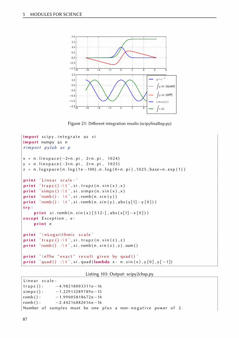
5 MODULES FOR SCIENCE

Figure 21: DiUerent integration results (scipyVnalbsp.py)

import s c i p y . i n t e g r a t e as s iimport numpy as n# impo r t py l ab as p

x = n . l i n s p a c e (−2∗n . pi , 2∗n . pi , 1 0 2 4 )y = n . l i n s p a c e (−2∗n . pi , 2∗n . pi , 1 0 2 5 )z = n . l o g spa c e ( n . l o g ( 1 e−100) , n . l o g ( 4∗ n . p i ) , 1 0 2 5 , base =n . exp ( 1 ) )

print ’ L i n e a r s c a l e : ’print ’ t r a p z ( ) : \ t ’ , s i . t r a p z ( n . s i n ( x ) , x )print ’ s imps ( ) : \ t ’ , s i . s imps ( n . s i n ( x ) , x )print ’ romb ( ) : \ t ’ , s i . romb ( n . s i n ( y ) )print ’ romb ( ) : \ t ’ , s i . romb ( n . s i n ( y ) , abs ( y[1]−y [ 0 ] ) )t ry :

print s i . romb ( n . s i n ( x ) [ 5 1 2 : ] , abs ( x [1]− x [ 0 ] ) )except Except ion , e :

print e

print ’ \ nLoga r i thmic s c a l e ’print ’ t r a p z ( ) : \ t ’ , s i . t r a p z ( n . s i n ( z ) , z )print ’ romb ( ) : \ t ’ , s i . romb ( n . s i n ( z ) , z ) . sum ( )

print ’ \ nThe " e x a c t " r e s u l t g i v en by quad ( ) ’print ’ quad ( ) : \ t ’ , s i . quad ( lambda x : n . s i n ( x ) , y [ 0 ] , y [−1])

Listing 103: Output: scipy2cbsp.pyL i n e a r s c a l e :t r a p z ( ) : −4 .98218003311 e−16simps ( ) : −1 . 22913289789 e−15romb ( ) : −1 .99005818672 e−14romb ( ) : −2 .44216882016 e−16Number o f samples must be one p l u s a non−nega t i v e power o f 2 .

87

5 MODULES FOR SCIENCE

Loga r i thm i c s c a l et r a p z ( ) : 0 . 7 8 1 0 8 2 0 5 7 6 5 9romb ( ) : 5 8 4 . 3 4 2 8 7 3 4 2 2

The " e x a c t " r e s u l t g i v en by quad ( )quad ( ) : ( 0 . 0 , 8 . 8 4 1 1 0 8 3 2 4 3 2 0 0 7 3 e−14)

5.3 MatPlotLib5.3.1 Plotting in 1D• matplotlib is the 2D plotting module for Python.

• The most important tools for creating plots are bundled in the pylab module.

⇒ Unless you are planning something really exotic, pylab will be suXcient.

Listing 104: Minimalistic Plot (pylabmin.py)# ! / u s r / b i n / env python

import py lab as p

x = p . arange (−4∗p . pi , 4 ∗ p . pi , . 1 )y = p . s i n ( x ) / x

p . p l o t ( x , y )p . show ( ) # or p . s a v e f i g ( " py labmin . png " )

• The plot command is the classical choice for xy plots. It can display multiple graphs in oneplot window. It can plot:

– a single array with y-values or

– pairs of arrays containing x- and y-values.

– additional plotting style deVnitions.

• More complex tools (e.g. event management for draggable and resizable object, changingscaling of the axes, etc.) are contained in the submodules ofMatPlotLib.

• Notice: We need the show() or saveVg() function to actually get a plot!

Listing 105: Example (pylab1bsp.py)# ! / u s r / b i n / env python

import py lab as p l

# i f f i g u r e ( ) i s om i t t e d py l ab a u t om a t i c a l l y# s t a r t s a new f i g u r e . I n py l ab f i g u r e s a r e# t h e e q u i v a l e n t t o windows .p l . f i g u r e ( )p l . s u bp l o t ( 1 , 2 , 1 )

88

5 MODULES FOR SCIENCE

Figure 22: Example on a minimalistic plot().

# B e i s p i e l : Histogramm + P l o tx = p l . randn ( 1 0 0 0 0 )n , b , p = p l . h i s t ( x , 3 0 , normed=True )y = p l . normpdf ( b , 0 , 1 )p l . p l o t ( b , y , ’ r−− ’ , lw =2 )

p l . s u bp l o t ( 1 , 2 , 2 )a = p l . a range (−1∗ p l . p i , 1 ∗ p l . p i , . 0 1 )p = p l . p l o t ( a , p l . cos ( 1∗ a ) ∗ p l . s i n ( 1 6∗ a ) )p l . l egend ( p , [ " $ \ cos ( x ) ∗ \ s i n ( 1 6 x ) $ " ] , 1 )p l . show ( )

• The subplot command arranges multiple plots in one Vgure. The Vrst two arguments deVnethe size (x,y) and the third argument speciVes the position of the current subplot.

• The hist plotting tool generated a histrogram from the data x using 30 bars/bins. The returnvalues are n (values), b (bins) and p (patch objects).

• normpdf evaluated the normed probability density function at b. Further arguments are µand σ.

• The legend command draws a legend. Therefore one needs to save the Line2D objects re-turned from the plot command.

• The plot command allows to customize the plotted lines. A formatting string following thedata in the arguments alters the appearance of the line:

89

5 MODULES FOR SCIENCE

Figure 23: Output (pylab1bsp.py)

’-’ solid line style ’b’ blue’–’ dashed line style ’g’ green’-.’ dash-dot line style ’r’ red’:’ dotted line style ’c’ cyan’o’ circle marker ’m’ magenta’v’ triangle down marker ’y’ yellow’s’ square marker ’k’ black’D’ diamond marker ’w’ white’d’ thin diamond markerFor a complete list of options see Reference Manual. If the desired color is not pre-deVned,you can deVne your own color using RGB-codes.

Listing 106: Example (pylabformatbsp.out)>>> import py lab as p>>> x = p . arange ( 0 , 2 ∗ p . pi , . 1 )>>> y = p . s i n ( x )>>> z = p . cos ( x )>>> p . p l o t ( x , y , ’om ’ , x , z , ’ b− . ’ )[ < ma t p l o t l i b . l i n e s . Line2D o b j e c t a t 0 x2262350 > , < ma t p l o t l i b . l i n e s .

Line2D o b j e c t a t 0 x202 f8d0 >]>>> p . x l a b e l ( ’X ’ )< ma t p l o t l i b . t e x t . Tex t o b j e c t a t 0 x225dcd0 >>>> p . y l a b e l ( ’Y ’ )< ma t p l o t l i b . t e x t . Tex t o b j e c t a t 0 x2260650 >>>> p . t i t l e ( ’ S inus und Cos inus ’ )< ma t p l o t l i b . t e x t . Tex t o b j e c t a t 0 x2260d10 >>>> p . g r i d ( )>>> p . show ( )

• Notice: Many pylab commands instantiate objects, which we use e.g. for writing legends.But they oUer much more possibilities!

• Among color and style of lines other properties – e.g. line width, opacity, . . . – can bechanged, too. Refer to plot manual.

90

5 MODULES FOR SCIENCE

Figure 24: Plot generated by listing 106.

5.3.2 Plotting in 2D

(a) Wireframe plot with older version (b) Contour and pseudo-color plot (see listing108)

Figure 25: DiUerent 3D plotting types.

• Until version 0.89 pylab had support for 3D representations of plots, e.g. wireframe plot.

• These features have been moved from pylab to a submodule: mplot3d

• But anything in 2D can be displayed using pylab: Contour plots and pseudo-color plots.

• For pylab’s 2D plots we need a somewhat more complex coordinate system than simple 1Darrays: 2D arrays we will call (mesh)grids.

91

5 MODULES FOR SCIENCE

Listing 107: Meshgrids for 2D plots>>> from numpy import meshgr id>>> X , Y = meshgr id ( [ 1 , 2 , 3 ] , [ 4 , 5 , 6 , 7 ] )>>> Xa r r ay ( [ [ 1 , 2 , 3 ] ,

[ 1 , 2 , 3 ] ,[ 1 , 2 , 3 ] ,[ 1 , 2 , 3 ] ] )

>>> Ya r r ay ( [ [ 4 , 4 , 4 ] ,

[ 5 , 5 , 5 ] ,[ 6 , 6 , 6 ] ,[ 7 , 7 , 7 ] ] )

• Meshgrids for 2D plots are nested structures, but there is an easy way of deVning them byusing the function meshgrid().

⇒ The meshgrid function takes the 1D coordinate axes – as we see in the example meshgridaccepts simple sequences, too – and transforms them into two 2D arrays.

• Most 2D plotting tools expect like the simple plot command information on the coordinatesystem – two meshgrids – and the data to plot.

• As colors do not carry Vxed values in diUerent plots a solution to this problem is also provided.

– To all pseudo-color plots a color bar can be added.

– In contour plots labels for contour lines can be added.

Listing 108: Example (pylab2bsp.py)# ! / u s r / b i n / env python

import py lab as p

x = p . arange (−2∗p . pi , 2∗p . pi , . 0 1 )X , Y = p . meshgr id ( x , x )Z = p . cos ( X ) ∗ p . s i n ( Y ) / Y

p . s ubp l o t ( 2 1 1 )p1 = p . contour ( x , x , Z )p . c l a b e l ( p1 )

p . s ubp l o t ( 2 1 2 )p . pco lormesh ( x , x , Z )p . c o l o r b a r ( )# No t i c e t h e i n c o n s i s t e n c y :# c l a b e l t a k e s an argument and# c o l o r b a r doe s no t !p . s a v e f i g ( ’ py l ab2 . png ’ )

92

5 MODULES FOR SCIENCE

• The Vgure() opens a new window in the interactive mode or allows to save a plot in a separateVle.

– Pylab automatically instantiates a Vgure, if no done by the programmer.

– Figures are counted beginning at 1.

⇒ In advanced programming of interactive Vgures, one can alter a speciVc Vgure!

– Possible arguments

num The number of the Vgure.Vgsize Size of the Vgure in inch as a sequence, e.g. (3,5).

dpi Resolution.facecolor Background color.edgecolor Border color.

• The subplot() command arranges multiple graphs in one Figure.

– subplot expects exactly 3 integer arguments.

1. Number of rows.2. Number of column.3. Current position.

⇒ Positions are counting beginning at 1 from left to right.

– If all three arguments are smaller than 10, the separation by coma is not required. E.g.(2,3,4) is equivalent to (234).

• plot() is a normal line plot.

– plot needs at least arrays with y-values. In thise case array indices are used for x-axisvalues.

– Alternatively pairs of arrays with x- and y-values can be speciVed.

– After a pair of arrays a plot formatting string can be given.

⇒ Arguments of plot follow this scheme: "x,y,format,x,y,format,. . . ".

• hist() plots a histrogram of a given array.

– Returns a tuple of the form (n,bins,patches); n are the histogram values, bins the numberof values and patches are equivalents to Line2D.

– Arguments

x Array.bins Number of "bins" or sequence of coordinates.

range Limits the range of x for evaluation and plotting.normed If True, result will be normed.weight Array with weighting factors.

∗ and much more.

• Remember to set the usetex option, if you want to use LATEX to render your text.

93

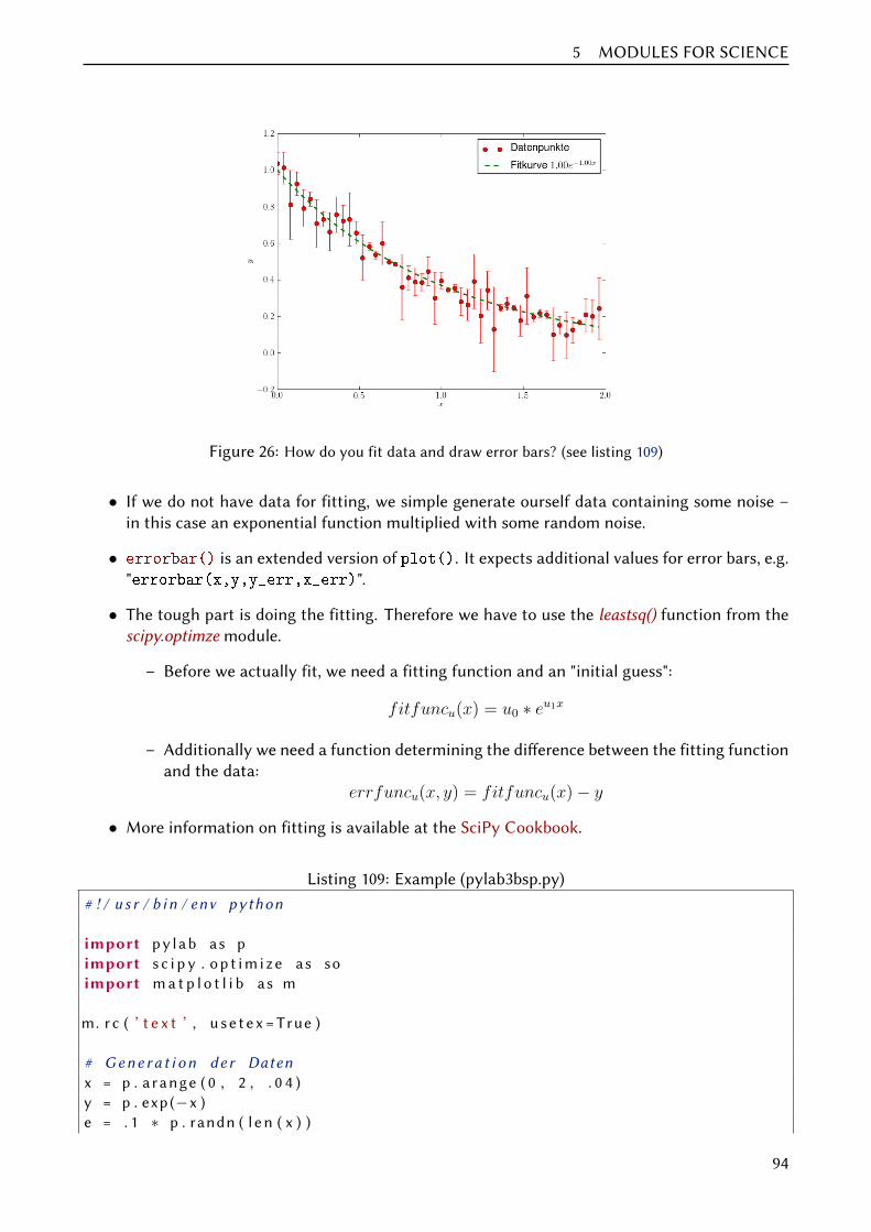
5 MODULES FOR SCIENCE

Figure 26: How do you Vt data and draw error bars? (see listing 109)

• If we do not have data for Vtting, we simple generate ourself data containing some noise –in this case an exponential function multiplied with some random noise.

• errorbar() is an extended version of plot(). It expects additional values for error bars, e.g."errorbar(x,y,y_err,x_err)".

• The tough part is doing the Vtting. Therefore we have to use the leastsq() function from thescipy.optimze module.

– Before we actually Vt, we need a Vtting function and an "initial guess":

fitfuncu(x) = u0 ∗ eu1x

– Additionally we need a function determining the diUerence between the Vtting functionand the data:

errfuncu(x, y) = fitfuncu(x)− y

• More information on Vtting is available at the SciPy Cookbook.

Listing 109: Example (pylab3bsp.py)# ! / u s r / b i n / env python

import py lab as pimport s c i p y . op t im i z e as soimport ma t p l o t l i b as m

m. r c ( ’ t e x t ’ , u s e t e x =True )

# Gen e r a t i o n de r Datenx = p . arange ( 0 , 2 , . 0 4 )y = p . exp (−x )e = . 1 ∗ p . randn ( l en ( x ) )

94

5 MODULES FOR SCIENCE

z = y + . 6 ∗ y . max ( ) ∗ e

# P l o t Daten mi t F e h l e r b a l k e nl 1 =p . e r r o r b a r ( x , z , abs ( e ) , None , fmt= ’ ro ’ )

# Funk t i on , mi t d e r g e f i t t e t w i rdf i t f u n c = lambda u , x : u [ 0 ] ∗ p . exp ( u [ 1 ] ∗ x )# Abweichung zw i s c h en Daten und F i t f u n k t i o ne r r f u n c = lambda u , x , y : f i t f u n c ( u , x ) − y# I n i t i a l w e r t e f u e r Pa r ame t e ru = [−1 , 10 ]# Lea s t−s qua r e f i t t i n gp1 , s u c c e s s = so . l e a s t s q ( e r r f unc , u , a r g s = ( x , y ) )

# P l o t d e r F i t f u n k t i o ny = p1 [ 0 ] ∗ p . exp ( p1 [ 1 ] ∗ x )l 2 =p . p l o t ( x , y , ’ g−− ’ , lw =2 )p . x l a b e l ( r ’ $x$ ’ )p . y l a b e l ( r ’ $y$ ’ )p . l egend ( ( l 1 [ 0 ] , l 2 ) , ( ’ Datenpunkte ’ , \

’ F i t k u r v e $ %5 .2 f e ^ { %5 .2 f x } $ ’ % ( p1 [ 0 ] , p1 [ 1 ] ) ) )p . show ( )

Notice:

• We start oU with a rather bad guess (-1,10).

• The leastsq() function tries to minimize the function that is passed to it and returns a se-quence of numbers that do minimize it.

• The leastsq() function also needs the data and the x-values for the fitfunc. These argumentsare passed through to errfunc and fitfunc.

• The arguments of errorbar() containing the information on how large to draw the error barscan be sequences or scalar numbers!

5.4 Mayavi• Matplotlib has never been designed to be a 3D plotting library.

• For true 3D visualization one has to use Mayavi (Docs) – a powerful 3D visualization toolwritten in Python.

• It can be used as simple as pylab to render plots and take a look at the output in an interac-tive window.

• In order to use all features of Mayavi one has to use its pipelines so that the application canwork on your data instead of just displaying it.

• Mayavi displays data (even less than 3D) in a 3D space

0D Points in space.

1D Space curves.

2D Surfaces.

3D Volumes and vector Velds.

95

5 MODULES FOR SCIENCE

Figure 27: 3D contour plot of 2p hydrogen orbitals and cylindrical distribution of magnetic mo-ments and magnetic Veld caused by these.

Figure 28: Examples

5.4.1 Mesh types• As we have seen Matplotlib uses so called dense or Weshed out mesh grids or coordinatematrices.

Listing 110: Example (mgrid.out)>>> import numpy>>> x = numpy . arange ( 5 )>>> xa r r ay ( [ 0 , 1 , 2 , 3 , 4 ] )>>> X , Y = numpy . meshgr id ( x , x )>>> X # f l e s h e d ou t meshg r i da r r ay ( [ [ 0 , 1 , 2 , 3 , 4 ] ,

[ 0 , 1 , 2 , 3 , 4 ] ,[ 0 , 1 , 2 , 3 , 4 ] ,[ 0 , 1 , 2 , 3 , 4 ] ,[ 0 , 1 , 2 , 3 , 4 ] ] )

>>> # A l t e r n a t i v e method o f c r e a t i o n. . . y , x = numpy . mgrid [ 0 : 5 , 0 : 5 ]>>> xa r r ay ( [ [ 0 , 1 , 2 , 3 , 4 ] ,

[ 0 , 1 , 2 , 3 , 4 ] ,[ 0 , 1 , 2 , 3 , 4 ] ,[ 0 , 1 , 2 , 3 , 4 ] ,

96

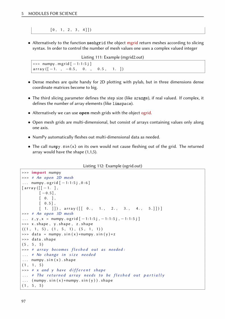
5 MODULES FOR SCIENCE

[ 0 , 1 , 2 , 3 , 4 ] ] )

• Alternatively to the function meshgrid the object mgrid return meshes according to slicingsyntax. In order to control the number of mesh values one uses a complex valued integer

Listing 111: Example (mgrid2.out)>>> numpy . mgrid [ −1 : 1 : 5 j ]a r r ay ( [ −1 . , −0 .5 , 0 . , 0 . 5 , 1 . ] )

• Dense meshes are quite handy for 2D plotting with pylab, but in three dimensions densecoordinate matrices become to big.

• The third slicing parameter deVnes the step size (like arange), if real valued. If complex, itdeVnes the number of array elements (like linspace).

• Alternatively we can use open mesh grids with the object ogrid.

• Open mesh grids are multi-dimensional, but consist of arrays containing values only alongone axis.

• NumPy automatically Weshes out multi-dimensional data as needed.

• The call numpy.sin(x) on its own would not cause Weshing out of the grid. The returnedarray would have the shape (1,1,5).

Listing 112: Example (ogrid.out)>>> import numpy>>> # An open 2D mesh. . . numpy . o g r i d [ −1 : 1 : 5 j , 0 : 6 ][ a r r ay ( [ [ −1 . ] ,

[ −0 . 5 ] ,[ 0 . ] ,[ 0 . 5 ] ,[ 1 . ] ] ) , a r r ay ( [ [ 0 . , 1 . , 2 . , 3 . , 4 . , 5 . ] ] ) ]

>>> # An open 3D mesh. . . z , y , x = numpy . o g r i d [ −1 : 1 : 5 j , − 1 : 1 : 5 j , − 1 : 1 : 5 j ]>>> x . shape , y . shape , z . shape( ( 1 , 1 , 5 ) , ( 1 , 5 , 1 ) , ( 5 , 1 , 1 ) )>>> data = numpy . s i n ( x ) ∗numpy . s i n ( y ) ∗ z>>> data . shape( 5 , 5 , 5 )>>> # a r r a y becomes f l e s h e d ou t as needed :. . . # No change i n s i z e needed. . . numpy . s i n ( x ) . shape( 1 , 1 , 5 )>>> # x and y have d i f f e r e n t shape. . . # The r e t u r n e d a r r a y need s t o be f l e s h e d ou t p a r t i a l l y. . . ( numpy . s i n ( x ) ∗numpy . s i n ( y ) ) . shape( 1 , 5 , 5 )

97

5 MODULES FOR SCIENCE

5.4.2 Plotting in 3D• Like Matplotlib (matplotlib.pyplot aka pylab) Mayavi provides a submodule mlab that isvery similar to pylab in usage.

• Depending on the version of Mayavi it is a stand-alone module or submodule in enthought.

• Syntax of the plotting commands plot3d and points3d is similar to pylab functions: Threecoordinate arrays and a scalar data array of the same shape.

• Figure completely conVgurable in display!

Figure 29: Output of meshes.py: Dots in 3D space and curve in 3D connecting the dots.

Listing 113: Example (meshes.py)# ! / u s r / b i n / env python

import numpyt ry :

from mayavi import mlabexcept :

from enthought . mayavi import mlab

t = numpy . l i n s p a c e ( 0 , 4 ∗ numpy . pi , 1 2 8 )x = lambda t : numpy . cos ( 3∗2∗numpy . p i ∗ t )y = lambda t : numpy . s i n ( 2∗numpy . p i ∗ t )z = lambda t : . 5 ∗ t ∗∗2

mlab . f i g u r e ( )mlab . po i n t s 3d ( x ( t ) , y ( t ) , z ( t ) , t , s c a l e _ f a c t o r = . 5 )

mlab . f i g u r e ( )mlab . p l o t 3d ( x ( t ) , y ( t ) , z ( t ) , t )mlab . show ( )

• Some Mayavi’s plot functions can be called only with the scalar/vector data.

• Elements (e.g. cut planes) can be added to the Vgure/scene by using the interactive pipelineeditor.

• Mayavi does not treat masked arrays correctly. Elements set to NaN are treated as masked inthe plots.

98

5 MODULES FOR SCIENCE

Figure 30: “Masked” mesh of 2p electron wave function.

Listing 114: Example (MayaHydro.py)# ! / u s r / b i n / env python

import numpy , s c i p y . s p e c i a lfrom mayavi import mlab

r = lambda x , y , z : numpy . s q r t ( x ∗∗2+y∗∗2+ z ∗∗2 )t h e t a = lambda x , y , z : numpy . a r c c o s ( z / r ( x , y , z ) )ph i = lambda x , y , z : numpy . a r c c o s ( x / r ( x , y , z ) ) ∗numpy . s i gn ( y )

a0 = 1 .R = lambda r , n , l : ( 2∗ r / n / a0 ) ∗∗ l ∗ numpy . exp (− r / n / a0 ) ∗ s c i p y . s p e c i a l .

g en l a gu e r r e ( n−l −1 ,2∗ l +1 ) ( 2∗ r / n / a0 )WF = lambda r , the ta , phi , n , l ,m: R ( r , n , l ) ∗ s c i p y . s p e c i a l . sph_harm (m, l , phi ,

t h e t a )

z , y , x = numpy . o g r i d [ − 2 4 : 2 4 : 6 4 j , − 2 4 : 2 4 : 6 4 j , − 2 4 : 2 4 : 6 4 j ]

# Why don ’ t I u s e a masked a r r a y ?mask = numpy . s e l e c t ( [ t h e t a ( x , y , z ) >numpy . p i / 3 . ] , [ numpy . s e l e c t ( [ abs ( ph i ( x , y

, z ) ) <numpy . p i / 3 . ] , [ numpy . nan ] , d e f a u l t =1 ) ] , d e f a u l t =1 )

for n in range ( 2 , 3 ) :for l in range ( 1 , n ) :

for m in range (− l , l + 1 , 1 ) :mlab . contour3d ( abs (WF( r ( x , y , z ) , t h e t a ( x , y , z ) , ph i ( x , y , z ) , n , l ,m)

) ∗∗2∗mask , con tou r s =6 , t r a n s p a r e n t =True )

mlab . c o l o r b a r ( )mlab . show ( )

• As we have seen previously Mayavi allows plotting without the explicit use of pipelines.

99

5 MODULES FOR SCIENCE

• For more elaborate functions of Mayavi one cannot avoid them.

• Pipeline Layout

Engine Represents the application; hidden in pipeline view.

Scene DiUerent Vgures.

Source The submodule mlab.pipeline can operate on diUerent data source objects, e.g. scalar_Veldand vector_Veld.

Filter Tools for transforming the data; mostly added to pipeline by functions, if needed.

Manager The module manager is automatically added to pipeline; controls color coding and leg-end.

Module Plot elements that are added to the scene, e.g. coordinate axes, cut planes, contour plot,...

Figure 31: Volumetric plot of sin(r)/r · cos(6φ) · e−z2

Listing 115: Example (pipebsp.py)# ! / u s r / b i n / env python

import numpyfrom mayavi import mlab

x , y , z = numpy . mgrid [−2∗numpy . p i : 2 ∗ numpy . p i : 6 4 j ,−2∗numpy . p i : 2 ∗ numpy . p i : 6 4 j, − 2 : 2 : 6 4 j ]

r = lambda x , y : numpy . s q r t ( x ∗∗2+y ∗∗2 )ph i = lambda x , y : numpy . a r c c o s ( x / r ( x , y ) ) ∗numpy . s i gn ( y )v = numpy . s i n ( r ( x , y ) ) / r ( x , y ) ∗numpy . cos ( 6∗ phi ( x , y ) ) ∗numpy . exp (−z ∗∗2 )

mlab . p i p e l i n e . volume ( mlab . p i p e l i n e . s c a l a r _ f i e l d ( v ) )mlab . show ( )

• One can create multiple scenes, where each scene can contain multiple sources (as seen inListing 114 and 113).

• Themodule manager is inserted after Vlters in the pipeline and can contain multiple modules.

• Let’s examine the pipeline of Listing 113.

100

5 MODULES FOR SCIENCE

Figure 32: Screenshot

• The script contains two scenes each with a data source.

• Scene 1

– The points3d function creates a data source

– and adds the glyph module to display the points.

• Scene 2

– The plot3d function creates a source made of points connected by lines.

– It applies the Stripper Vlter, which transforms this succession of lines in a “strip”.

– Another Stripper Vlter creates tubes with a given radius from the strip.

– The Surface module is applied to display the surface of the tubes.

Figure 33: Magnetic Veld caused by magnetic moments.

101

5 MODULES FOR SCIENCE

• Vector plots can be done in two ways.

– With the function quiver3d. Vector components are given as separate arguments.

– Manual pipeline construction

∗ vector_Veld data source.∗ The module vectors makes a voluminous vector plot.∗ The module vector_cut_plane produces an interactive cut plane in which the vec-tors are drawn.

• In most cases one can add elements to the pipe generated by a plot function.

• In more complicated cases, e.g. interactivly adding a vector cut plane to a quiver3d pipeline,this does not work.

• One has to set up the pipeline manually in the script.

• In the treatment of large data sets parallization is useful. For this task threading (see Chapter4.1)

and multiprocessing are very useful.

• The following example Listing 116 is not written in the most elegant way. In an elegantsolution all values required in the worker function would be passed as arguments to thefunction.

Listing 116: Example (vectorfull.py)# ! / u s r / b i n / env python

import t imeimport sysimport os . pathimport numpyimport mayavi . mlabimport Queueimport s c i p y . f f t p a c k as f f t p a c kimport mu l t i p r o c e s s i n g

use_saved = True

def worker ( mys l i ce , q , A ) :i f mys l i c e [ 1 ] >= A . shape [ 1 ] :

mys l i c e [ 1 ] = A . shape [1]−1

for a in range ( mys l i c e [ 0 ] , mys l i c e [ 1 ] ) :for b in range (A . shape [ 2 ] ) :

for c in range (A . shape [ 3 ] ) :# ra i s t h e p o s i t i o n where t h e f i e l d s s h a l l be# c a l c u l a t e d .ra = numpy . a r r ay ( [ x [ a , b , c ] , y [ a , b , c ] , z [ a , b , c ] ] )

# C a l c u l a t i o n o f t h e v e c t o r p o t e n t i a l and magne t i c

102

5 MODULES FOR SCIENCE

# f i e l d .a_sum = numpy . a r r ay ( ( 0 , 0 , 0 ) , dtype= ’ f l o a t ’ )for d in range (m. shape [ 1 ] ) :

for e in range (m. shape [ 2 ] ) :for f in range (m. shape [ 3 ] ) :

rm = numpy . a r r ay ( ( x [ d , e , f ] , y [ d , e , f ] , z [ d , e , f ] ))

M = m[ : , d , e , f ]R = ra − rmcube = be t r ag ( R ) ∗∗3i f cube . a l l ( ) ! = 0 :

a_sum += kreuzp rodukt (M, R ) / cubee l se :

a_sum += numpy . z e r o s ( 3 )A [ : , a , b , c ] = a_suma_sum = numpy . z e r o s _ l i k e ( a_sum )

q . put ( ( mys l i ce , A ) )print " F i n i s h ed ! "return None

def p a r t i a l (A , x =0 ) :" C a l c u l a t e p a r t i a l d e r i v a t i v e o f a 3D py lab a r r ay a long one a x i s . "

A_prime = numpy . z e r o s _ l i k e (A )l = l i s t (A . shape )i f l e n ( l ) > x : del l [ x ]

for i in range ( l [ 0 ] ) :for j in range ( l [ 1 ] ) :

i f x ==0 :s = A [ : , i , j ] . copy ( )A_prime [ : , i , j ] = f f t p a c k . d i f f ( s )

e l i f x ==1 :s = A[ i , : , j ] . copy ( )A_prime [ i , : , j ] = f f t p a c k . d i f f ( s )

e l i f x ==2 :s = A[ i , j , : ] . copy ( )A_prime [ i , j , : ] = f f t p a c k . d i f f ( s )

e l se :ra i s e Va lueE r ro r , "No v a l i d d i r e c t i o n : %s " % x

return A_prime

def be t r ag ( a ) :return numpy . s q r t ( abs ( numpy . dot ( a , a ) ) )

def kreuzp rodukt ( a , b ) :tmp = numpy . a r r ay ( [

a [ 1 ]∗ b [ 2 ] − a [ 2 ]∗ b [ 1 ] ,a [ 2 ]∗ b [ 0 ] − a [ 0 ]∗ b [ 2 ] ,a [ 0 ]∗ b [ 1 ] − a [ 1 ]∗ b [ 1 ]

103

5 MODULES FOR SCIENCE

] )

return tmp

d a t a _ f i l e = " v e c t o r _ f i e l d _A _ _ sw i t c h _mu l t i p r o c . npy "

# Queue f o r s p l i t t i n g t h e A compon t en t s f o r p a s s i n g t o Th r ead s# Shape o f queue e l emen t s : [ beg in , end ]t ry :

max_threads = mu l t i p r o c e s s i n g . cpu_count ( )except Except ion , e :

print emax_threads = 2

print "No o f P r o c e s s e s : " , max_threads# The c o o r d i n a t e g r i dx , y , z = numpy . mgrid [ −6 : 6 : 1 7 j , − 6 : 6 : 1 7 j , − 6 : 6 : 9 j ]

# The d i s t r i b u t i o n o f magne t i c momentsm = numpy . a r r ay ( [

numpy . z e r o s _ l i k e ( x ) ,numpy . z e r o s _ l i k e ( y ) ,numpy . s e l e c t ( [ x ∗∗2+y ∗∗2 <9 ] , [ numpy . s e l e c t ( [ abs ( z ) <2 , abs ( z ) >=2 ] , [ numpy .

s i gn ( x ) , 0 ] ) ] )] )

i f use_saved and os . path . i s f i l e ( d a t a _ f i l e ) :A = numpy . l oad ( d a t a _ f i l e )

e l se :# The magne t i c v e c t o r p o t e n t i a lA = numpy . z e r o s _ l i k e (m)a = A . shape [ 1 ] / max_threads +1q = mu l t i p r o c e s s i n g . Queue ( )for i in range ( max_threads ) :

mys l i c e = [ i ∗a , i ∗a+a ]print mys l i c ew = mu l t i p r o c e s s i n g . P r o c e s s ( t a r g e t =worker , a r g s = ( mys l i ce , q , A ) )w . s t a r t ( )

t ime . s l e e p ( 6 0 )q I tems = 0while mu l t i p r o c e s s i n g . a c t i v e _ c h i l d r e n ( ) :

t ime . s l e e p ( 5 )print q . q s i z e ( )t ry :

mys l i ce , A2 = q . ge t ( True , t imeout =10 )except Except ion , e :

print " Caught e x c ep t i o n : " , ei f qItems >=max_threads : break

qItems += 1i f mys l i c e [1 ] > A . shape [ 1 ] : mys l i c e [ 1 ] = A . shape [1]−1print mys l i c e

104

5 MODULES FOR SCIENCE

A [ : , mys l i c e [ 0 ] : mys l i c e [ 1 ] , : , : ] = A2 [ : , mys l i c e [ 0 ] : mys l i c e [ 1 ] , : , : ] .copy ( )

numpy . save ( d a t a _ f i l e , A )

B = [p a r t i a l (A [ 1 ] , 2 ) − p a r t i a l (A [ 2 ] , 1 ) ,p a r t i a l (A [ 2 ] , 0 ) − p a r t i a l (A [ 0 ] , 2 ) ,p a r t i a l (A [ 0 ] , 1 ) − p a r t i a l (A [ 1 ] , 0 )

]

mayavi . mlab . f i g u r e ( s i z e = ( 1 2 8 0 , 8 0 0 ) )# Us ing p l o t f u n c t i o n smayavi . mlab . qu i v e r 3d ( x , y , z ,m[ 0 ] ,m[ 1 ] ,m[ 2 ] , name= " Magnet ic Moments " )# mayavi . mlab . q u i v e r 3 d ( x , y , z , A [ 0 ] , A [ 1 ] , A [ 2 ] , name =" V e c t o r P o t e n t i a l " )# mayavi . mlab . q u i v e r 3 d ( X , Y , Z , B [ 0 ] , B [ 1 ] , B [ 2 ] , name =" Magne t i c F i e l d " )# C r e a t i n g t h e p l o t u s i n g t h e p i p e l i n es r c = mayavi . mlab . p i p e l i n e . v e c t o r _ f i e l d ( x , y , z , B [ 0 ] , B [ 1 ] , B [ 2 ] , name= "

Magnet ic F i e l d " )magnitude = mayavi . mlab . p i p e l i n e . e x t r a c t _ v e c t o r _no rm ( s r c )f i e l d _ l i n e s = mayavi . mlab . p i p e l i n e . s t r e am l i n e ( magnitude , s eed type = " l i n e " ,

i n t e g r a t i o n _ d i r e c t i o n = " both " )# mayavi . mlab . p i p e l i n e . v e c t o r s ( s r c , ma s k_po i n t s =1 , s c a l e _ f a c t o r = 2 . )# mayavi . mlab . p i p e l i n e . v e c t o r _ c u t _ p l a n e ( s r c , ma s k_po i n t s =1 , s c a l e _ f a c t o r

= 2 . )

mayavi . mlab . o u t l i n e ( )mayavi . mlab . c o l o r b a r ( )mayavi . mlab . show ( )# mayavi . mlab . s a v e f i g ( " b l a . png " )

105

6 EXERCISES

6 Exercises6.1 The Basics

1. Interactive Shell. Start oU with getting comfortable with the Python shell. Look at thecontents of some modules, e.g. dir(math), or at the documentation on an object, e.g.help(int) or help(list).

2. Write a program that identiVes every number between two limits that is divisible by 7.

3. Write a program to convert Celsius⇔ Fahrenheit. Try diUerent method for passing data tothe script:

• Prompting input on the shell.

• Accepting arguments passed during script calling.

• Reading data from a Vle.

4. Calculate and print the Fibonacci series: F0 = 1, F1 = 1, Fn = Fn−1 + Fn−2

5. Write a program which determines whether a given year is a leap year or not.

• A year is a leap year, if it divisible by 4 unless

• it is divisible by 100. In this case it is not a leap year, unless

• it is divisible by 400.

6. DeVne yourself a list containing several elements (diUerent value!). Find an elegant way ofdeleting a speciVc element from the list. Tip: index().

6.2 Advanced I1. List Comprehensions

(a) Many programming language know the concept of stacks. Python has its own equiv-alent (Queue), but write your own version of a stack. It should emit exceptions, if it’sempty or full.

(b) In yesterday’s exercise 5 we determined whether a year was a leap year. Try to accom-plish the same task using list comprehensions.

(c) When working with large data, e.g. larger than 10000 elements, one should considera less memory consuming alternative: Generator Expressions. Try to solve the lastexercise using generator expressions.

2. Hamster – Write a script containing a hamster and a board object. The hamster shall movein a pattern and avoid obstacles on the board. Finally the board should have means to displaythe hamster’s motion.

3. Polynom – DeVne a class for polynomials. One shall be able to deVne, derive, integrate anddo math with polynomials. Do not use tools from the module numpy.

4. Rational numbers – Design a class for rational numbers allowing the four arithmetics. Thisclass shall also be able to return the reduced fraction or a Woat. Remember:

• A fraction can be fully reduced by dividing numerator and dominator by the greatestcommon divisor.

• Rational numbers are presentated as a fraction p/q, where p ∈ Z and q ∈ N\0.

106

6 EXERCISES

6.3 Advanced II1. Threading – Write a threaded script for retrieving (or generating), processing (e.g. apply a

function) and saving values. But do not forget:

• Instead of starting a thrad for each value, one can assign threads to tasks and passvalues to them using queues.

• Some operations, e.g. I/O, are not "thread-safe". Make sure nothing can go wrong.

• It can be annoying, if one tries to stop a threaded program, but it continues to run.Make sure the user can abort the program at any point.

2. Calculator – Write a calculator GUI using Tk. The user shall be able to choose a functionname (RadioButtons?) and enter a value, which shall be passed to the function, in a separatewindow (TopLevel?). The shall be closed, if the value is OK, and the result shall be displayedin the initial window.

3. Write a simple Tic-Tac-Toe game using Tk. But do not forget to save important data, e.g.which Veld has been hit by which player!

4. Write a script for managing a phone book. Write a GUI for managing entries and export/im-port to/from a Vle or database.

5. Racetrack – Write a threaded script for simulating a horse race. Horses shall be indepen-dently moved forward and the progress shall be displayed in a GUI, where also the winnershall be announced.

6.4 Numerical Computations1. Arrays – Getting used to

(a) Create a 3× 3-array with arbitrary values 6= 0 and resize it to a 9× 6 array.

(b) Assign am× n-slice (m,n 6= 0, 1,m 6= n) of the array to a variable.

(c) Set all elements of the slice equal 32π

(d) DeVne an array with length 100 for each property:

• Distance between elements is logarithmic.

• The array is empty.

(e) Resize your 9× 6 array to a 4× 13 array and to a 1-dim. array.

(f) We have seen select and piecewise. What is the diUerence between them andwhere?

2. Matrices

(a) Convert one of your 2-dim. arrays into a matrix.

(b) Create another matrix (same shape) using MatLab syntax.

(c) Perform addition and multiplication with those matrices. Convert matrices to arraysand repeat.

107

6 EXERCISES

(d) Solve the linear matrix equation:

v = A ∗

xyz

, v =

4−513

,

A =

1 0 −12 5 3−4 0 1

3. Polynomials

(a) Write a script for determining the roots and extrema – both x- and y- values – of apolynomial. Use e.g. this polynomial:

f(x) =1

3x5 − 2x2 − 6πx− 10

(b) Write a script for reading (x, y)-pairs from a Vle and Vtting with a polynomial p. De-termine the followin integral: ∫ π/3

0

p(x) dx

Highlight the integration limits using a patch.

Display your results graphically.

4. Add to your script from exercise 3b error bars.

5. Integral and DiUerential

(a) Write your own functions for integrating and deriving 1-dimensional arrays. Compareyour results with the results of the SciPy tools.

(b) Expand your previous script such it can derive 2-dimensional arrays:

Total :d

dxif(~x), i = 1, 2, . . .

Partial :

(∂

∂x1+

∂

∂x2+ . . .

)f(~x)

(c) [optional] Expand your script to interactively adjust the integration limits.

6. Fourier Transformation

(a) Write a script for expanding fourier series to Vt a given function/array.

(b) Expand the script to display a "Fourier spectrum"

Remember: A Fourier series looks like this:

f(t) =a02

+∞∑k=1

(ak · cos(kωt)

+ bk · sin(kωt))

an =2

T

∫ c+T

c

f(t) · cos(nωt) dt

bn =2

T

∫ c+T

c

f(t) · sin(nωt) dt

108