SCIENTIFIC COMMITTEE SEVENTH REGULAR SESSION [CPUE skipjack... · SCIENTIFIC COMMITTEE SEVENTH...
17
SCIENTIFIC COMMITTEE SEVENTH REGULAR SESSION 9-17 August 2011 Pohnpei, Federated States of Micronesia CPUE of skipjack for the Japanese offshore pole and line using GPS and catch data WCPFC-SC7-2011/SA-WP-09 (Rev.1) Suguru OKAMOTO 1 and Hidetada KIYOFUJI 1 1 National Research Institude of Far Seas Fisheries, Japan
Transcript of SCIENTIFIC COMMITTEE SEVENTH REGULAR SESSION [CPUE skipjack... · SCIENTIFIC COMMITTEE SEVENTH...

SCIENTIFIC COMMITTEE
SEVENTH REGULAR SESSION
9-17 August 2011
Pohnpei Federated States of Micronesia
CPUE of skipjack for the Japanese offshore pole and line using GPS and catch data
WCPFC-SC7-2011SA-WP-09 (Rev1)
Suguru OKAMOTO1 and Hidetada KIYOFUJI
1
1 National Research Institude of Far Seas Fisheries Japan
CPUE of skipjack for the Japanese offshore pole and line using GPS and catch data
Suguru OKAMOTO1 and Hidetada KIYOFUJI
1
1 National Research Institude of Far Seas Fisheries
Abstract
To create the new CPUE based on the fishing effort for searching skipjack fishing ground or
fish school GPS data loggers were deployed on 7 Japanese pole and line vessels(lt 200 GRT)
from July to September 2010 The position and speed of vessels were logged in every 1 second
Start and end time of fishing (angling) and skipjack catch (ton) of each fishing activities were
recorded on the field note by the fishing master The characteristic of vessel behavior of cruising
searching and fishing was investigated using these data Then the daily distances for searching
fishing ground were calculated and considered as a candidate of the fishing effort The classical
fishing effort (poleday derived from logbook data) was constant in each vessel while the new
fishing effort (distancepoleday in this study) varied several times from day to day The
variation and its pattern of the new CPUE were different from those of the classical CPUE It is
suggested from dataset in this study that the classical CPUE is more overestimated or
underestimated when daily catch is from 10 to 25 ton Therefore new CPUE would be effective
for the CPUE estimation particularly at its range of daily catch
Introduction
Skipjack tuna (Katsuwonus pelamis) lives in wide area within almost whole of the Pacific
Ocean (eg Matsumoto et al 1984) and skipjack catches is largest in the tropical region
(Williams and Terawasi 2010) According to the last skipjack stock assessment in 2010
although stock status of skipjack tuna has declined somewhat in recent years skipjack is not
overfished and its stock keeps still safe level even though total catch has been increasing On the
other hand recent skipjack catches near Japanese water north of 20degN has been decreasing
especially in 2009 it is lowest in 10 years Therefore it is pointed out that the skipjack migrating
seasonally to near the Japanese coastal waters may decrease (Uosaki et al 2010) Japanese
fishermen also have pointed out ldquothe decrease of skipjack school which they can find near
Japanese waterrdquo and they have been deeply concerned with the declining of skipjack stock
However its indication is not reflected in the latest stock assessment because the fishing effort
for finding skipjack school is not considered in CPUE used in the stock assessment Current
fishing efforts are the numbers of pole and day from logbook which donrsquot include the fishing
effort spent for searching fishing ground In this document we evaluated the new fishing effort
for searching fishing ground using GPS and catch data of Japanese pole and line vessels after
investigated vessel behavior and estimated CPUE which can reflect skipjack stock more from
its effort
Data and Methods
GPS data loggers were deployed on 7 Japanese pole and line vessels (lt 200 GRT) from July
to November 2010 (Table 1) During this period the vessels had been fishing in the east of Japan
(Fig 1) and the total of fishing day was 61 The position and speed of vessels were logged in
every 1-second Start and end time of fishing and skipjack catch (ton) of each activities were
recorded on the field note We checked the GPS data against the field note and identified the
fishing position To evaluate the new fishing effort the characteristic of vessel behavior at
fishing and searching fishing ground was investigated using these data To smooth short-term
fluctuations we calculated the 1-minute running mean and 5-minute running standard deviation
of vessel speed (RMspeed and RSDspeed respectively) and 1-minute running standard deviation of
bearing change per second (RSD∆bearing) The daily averaged speed and total distance for
searching fishing ground (DSFG) were also calculated The DSFG was considered as new fishing
effort which also meant to consider the density of skipjack school because DSFG should be short
when the frequency of finding the school was high Then the new CPUE (effort
distancepoleday) CPUEGPS was calculated and compared with the classical CPUE
CPUEclassical after normalized by mean and variance
Results and Discussion
To investigate the vessel behavior at fishing and searching fishing ground firstly the fishing
trip trajectories from the GPS data were mapped with catch data from the field note Figure 2
shows a trajectory of vessel ldquoCrdquo on August 4 On this day fishing and searching fishing ground
was started from 355 and finished at 1403 before went to the port for catch landing Fishing
mostly continued for more than 5 minutes when some catches (eg from 417 to 630 in Fig 2)
While fishing time were less than about 5 minutes when no catch only cast a bait (eg from
920 to 925 in Fig 2) and the vessel quickly shifted to searching next fishing ground When
the vessel found and arrived at fishing ground it rapidly slowed down (RMspeed lt about 10
kmhr) and kept low speed with casting bait for fishing (upper line in Figure 3) After fishing it
rapidly speeded up (RMspeed gt 20 kmhr) RSDspeed change rate of vessel speed increased to
more than 5 kmhr at the start and end of fishing (middle line in Figure 3) Using these
characteristics of vessel speed we will be able to extract ldquosearchingrdquo and ldquofishingrdquo
automatically RSD∆bearing change rate of vessel bearing also had signals to determine the vessel
behavior which it was high (ge about 10 ˚sec) during ldquofishingrdquo and low (lt about 10 ˚sec)
during ldquosearchingrdquo (lower line in Figure 3) And RSD∆bearing decreased exponentially with vessel
speed obviously (Figure 4)
Daily DSFG were calculated and considered as new fishing effort Temporal variability in the
fishing effort including DSFG EGPS (distancepoleday) was investigated Figure 5 shows the
time-series in EGPS of vessel ldquoDrdquo as an example The ratio between the maximum (443 on
September 5) and minimum (172 on August 20) values of EGPS was 26 and its coefficient of
variation was 26 while the classical fishing effort Eclassical (poleday) was constant Then
CPUEGPS was calculated using EGPS and compared with CPUEclasscail after normalized by mean
and variance (Figure 6) Trends in two CPUEs look similar however some differences were
observed in them variations For example on August 5 CPUEGPS was fourth-largest in all
CPUEGPS while CPUEclassical was second-largest in all CPUEclassical (Figure 6) CPUEGSP of all
vessels were also compared with CPUEclassical (Figure 7) There was a positive correlation
between two CPUEs (r2 = 090 p lt 00001) The relationship was strong especially when
CPUEclassical was less than 1 however its relationship was not shown when CPUEclassical was
from 1 to 3 Simply thinking this was because CPUEGPS should be more influenced by variation
in DSFG (denominator of CPUEGPS) when catch (numerator of CPUE) was higher (ie when
CPUEclassical was higher) It should be highly possible that CPUEclassical is more overestimated or
underestimated when catch is higher Focusing on this point we investigated the relationship
between DSFG and catch (Figure 8) Although there may be a bias of sample number DSFG
tended to be narrowly distributed with catch This would roughly make sense because DSFG
might decrease with catch which was positively correlated with fishing time (Figure 9) and a
certain amount of DSFG (gt about 70 km in Fig 8) is commonly needed for a certain amount of
catch (about gt 8 ton in Fig 8) To examine its relationship quantitatively the distributions of
DSFG were statistically processed at every 10 ton (Figure 10) The 95 upper prediction limits
linearly decreased with catch and the lower limit of that was smallest at a class from 10 to 20
ton and increased to the higher catch class Using the probability distribution of DSFG the
predicted distribution of CPUE was estimated roughly (Figure 11) When catch is more than 30
ton although CPUEGPS cannot be statistically predicted because of only one sample it is
assumed that the lower limit of CPUE would not greatly decrease (eg one-half) because DSFG
would not greatly increase (eg twice) at high catch On the contrary it is assumed that the
upper limit of CPUE would be higher at high catch because the lower DSFG could well occur
Especially when catch is from 10 to 25 it would be highly significant to estimate CPUEGPS
because the predicted CPUEGPS was distributed widely in Fig 11 However it is necessary that
GPS research are more conducted in peak season for fishing because samples at more than 5 ton
catch are particularly not enough to analyze statistically
In the next step we are planning to estimate the efforts for searching fishing ground from
past data We will use the data based on the onboard catch information exchange between
vessels and fuel consumption as a function of ldquosearchingrdquo and recalculate the past CPUE based
on the effort for searching fishing ground And we will be able to estimate the near real-time
spatial distribution of skipjack school density around the main fishing ground by extracting the
ldquofishingrdquo pattern of vessel behavior and its duration time using only GPS data
Acknowledgement
We thank the crews of the Japanese pole and line vessels and the National offshore Tuna
Fisheries Association of Japan for cooperating in the GPS research
References
Matsumoto W M Skillman R A and Dizon A E (1984) Synopsis of biological data on
skipjack tuna Katsuwonus pelamis NOAA Tech Rep NMFS Circ 451 1-92
Uosaki K Kiyofuji H Hashimoto K Okamoto S and Ogura M (2010) Recent status of
Japanese skipjack fishery in the vicinity of Japan WCPFC-SC6-2010 Nukualofa Tonga
SA-WP-07
Williams P and Terawasi P (2010) Overview of Tuna Fisheries in the western and central
Pacific Ocean including economic conditions-2009 WCPFC-SC6-2010 Nukualofa Tonga
GN-WP-01
Table 1 Period of GPS research and the number of fishing day in each vessel
Vessel ID Start day End day No of fishing day
(No of sample)
A 7152010 7282010 8
B 7292010 7302010 2
C 842010 852010 2
D 812010 982010 19
E 932010 982010 3
F 942010 10282010 11
G 1062010 1162010 16
Figure 1 Fishing trip trajectory of all pole and line vessels in this document
Figure 2 A fishing trip trajectory started from 355 and finished at 1403 on August 5 2010
Lines show the searching fishing ground Circles indicate that there were some catches (ton) and
triangles indicate no catch only bait casting
Position on Aug 5thー Searching fishing ground Some catches No catch (only bait casting)
S
E
355
417-630
(5t)
718-749
(4t)
930-935
(none)
1156-1157
(none)
1129-1139
(01t)1216-1221
(none)
1233-1240
(01t)
1403
920-925
(none)
Aug 5th
Figure 3 Time-series of the vessel behavior on August 5 2010 (Fig 2) Upper middle and
lower lines indicate the 1-minute running mean and 5-minute running standard deviation of
vessel speed (RMspeed and RSDspeed) and 1-minute running standard deviation of bearing change
per second (RSD∆bearing) respectively Shaded boxes and arrows indicate the time zones when
fishing was operated regardless of catch and when vessel was searching fishing ground
respectively
417-630(5t)
718-749(4t)
920-925(none) 1129-1139
(01t)
1156-1157(none)
1216-1221(none)
1233-1240(01t)
930-935(none)
searching searchingsearching searching searching
Figure 4 Relationship between the RMspeed and RSD∆bearing on August 5 2010 (Fig 2) with
frequencies of those two parameters
RMspeed (kmhr)
RS
D∆bearing(˚sec)
Fre
qu
en
cy o
f R
Msp
ee
d(
)
Frequency of RSD∆bearing ()
Figure 5 Comparison of temporal variability in the new fishing effort (distancepoleday) EGPS
and classical fishing effort (poleday) Eclassical using vessel ldquoDrdquo data EGPS is normalized by
mean and variance
Figure 6 Comparison of trends in the new CPUE considered distance as fishing effort and
classical CPUE using one vesselrsquos data These CPUEs are normalized by mean and variance
Figure 7 Comparison of normalized CPUEclassical and CPUEGPS (r2 = 090 n = 61 p lt 00001)
Linear line is the one-to-one line
Figure 8 Scatter plot showing the relationship between daily DSFG and catch
Figure 9 Linear regression describing the relationship between daily fishing time and catch (r2
= 075 n = 61 p lt 00001)
Figure 10 Box plot of daily DSFG versus catch at every 10 ton Boxes and vertical lines in the
boxes show the 25th and 75th percentiles and medians respectively Circles asterisks and
horizontal lines indicate means 1st and 99th percentiles and 95 prediction intervals
respectively The width of the boxes shows the number of sample for the box
Figure 11 Predicted distribution of CPUEGPS against catch and CPUEclassical estimated from the
probability distribution of DSFG in Fig 10 (shaded zone) Upward and downward triangles show
the catch and CPUEclassical versus CPUEGPS at the 95 upper and lower prediction limits of DSFG
respectively Curve lines are B-spline curves Circle indicates that sample is only one in the
catch class (gt 30 ton) and for that the curves connected to the circle are drawn by broken lines
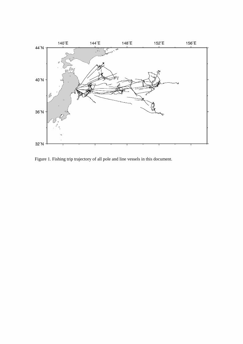
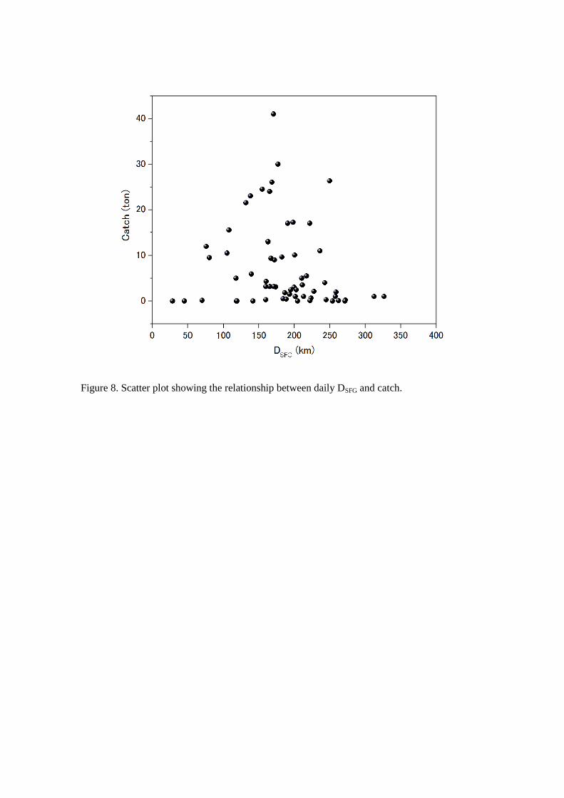
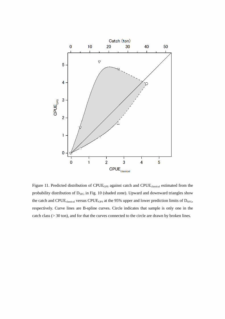