Observations and Numerical Simulation of Water Vapor Oscillation Events During

the International H2O Project (IHOP_2002)

Robin L. Tanamachi

School of Meteorology, University of Oklahoma, Norman, Oklahoma

Wayne F. Feltz

Cooperative Institute for Meteorological Satellite Studies, University of Wisconsin –

Madison, Madison, Wisconsin

Ming Xue

Center for Analysis and Prediction of Storms and School of Meteorology, University of

Oklahoma, Norman, Oklahoma

To be submitted to

Monthly Weather Review

14 March 2007

Corresponding author address:

Robin Tanamachi

University of Oklahoma

School of Meteorology

120 David L. Boren Blvd., Suite 5900

Norman, OK 73072-7307

rtanamachi@ou.edu

ABSTRACT

On the morning of 12 June 2002, a series of boundary layer water vapor

oscillation events occurred at the “Homestead” site of the International H2O Project

(IHOP_2002). Atmospheric water vapor magnitude within the boundary layer decreased

and increased within a matter of minutes. High temporal-resolution data of the water

vapor oscillations collected by an array of instruments deployed for this intensive

observation period are presented. The results of an Advanced Regional Prediction System

(ARPS) mesoscale numerical simulation of the weather conditions around the time period

in question are also discussed. The ARPS model reproduced the water vapor oscillations

with a remarkable accuracy. Both the observational data and ARPS numerical model

output indicate that the water vapor oscillations were due to interaction between a dry air

mass descending from the Rocky Mountains and a cold pool/internal undular bore

couplet propagating over the Homestead site from a mesoscale convective complex to the

north. The water vapor oscillations are believed to be a secondary indicator of such bores.

This type of water vapor oscillation was observed at other times during IHOP_2002, and

the oscillations are believed to be a relatively rare occurrence.

1. Introduction

During the intensive observation period from 13 May to 25 June 2002 of the

International H2O Project (IHOP_2002), a large array of in situ, mobile, and aircraft-

mounted water vapor sensing instruments from many institutions took collaborative water

vapor measurements over the central United States (Weckwerth et al. 2004, 2006). One

of the specified objectives of IHOP_2002 was “improved characterization of the four-

dimensional (4-D) distribution of water vapor and its application to improving the

understanding and prediction of convection.” Owing to the intensive nature of the

observation period, it was also possible to investigate the converse in some detail.

It has long been known that convective systems can generate “cold pools” that

can propagate like a density current across the surface (Bluestein 1993, p. 441; Houze

1993, p. 477). The passage of the gust front at the leading edge of this cold pool is often

characterized by a pressure jump and wind shift. Under stably stratified conditions, a bore

(Simpson 1987) may also develop and propagate ahead of the gust front. An observer

may experience alternating pressure rises and falls as the “ripples” of the bore pass by. At

an observation point above the surface, the properties of the air may alternate between

two states – with different temperatures, humidities, or wind speeds and directions –as

the bore passes. Bores generally contain regions of rising and sinking air motion, and can

potentially serve as convective triggers (Koch et al. 1991).

Herein, we describe the occurrence of four sharp, above-surface water vapor

oscillations that occurred during the IHOP_2002 intensive observation period (IOP), on

the morning of 12 June 2002. Several IHOP_2002 instruments at the “Homestead” site

near Balko, Oklahoma (in the Oklahoma panhandle) recorded detailed data during these

events. The boundary layer water vapor oscillations are best illustrated by the time-height

plot of water vapor profiles measured by the Atmospheric Emitted Radiance

Interferometer (AERI, Fig. 1, Feltz et al. 2003a and 2003b, Knuteson et al. 2004a and

2004b). High-resolution numerical simulations are performed for this event using the

non-hydrostatic ARPS (the Advanced Regional Prediction System) model (Xue et al.

2000, 2001, and 2003). The model reproduced two of the water vapor oscillations with

the near the right strengths, and reproduced the remaining two with somewhat weaker

strengths, all with remarkably accurate timings. It is suggested that these oscillations

were a secondary product of a nearby bore.

The synoptic environment around the time of the water vapor oscillation events is

described in Section 2. A description of data collected during this event is given in

Section 3. The ARPS numerical simulation of the event is described in Section 4.

Possible causes of the events are discussed in Section 5; a summary and conclusions are

then given in Section 6.

2. Synoptic environment of 12 June 2002

At 00 UTC, a weak upper level jet maximum (not shown) extended from eastern

Wyoming to western Nebraska. An area of relatively high velocities at 300 hPa stretching

southward into Colorado produced an upper-level region of decreasing (towards the east)

wind speeds across the Oklahoma panhandle. Atmospheric soundings from Dodge City,

Kansas and Amarillo, Texas at 00 UTC (Fig. 2) indicate that the atmospheric boundary

layer was well-mixed (with dry adiabatic temperature and constant water vapor profiles

in at least the lowest 200 mb) and neutrally stable at both sites. The westerly winds aloft

were stronger at Dodge City than at Amarillo, while the surface winds were

southwesterly at Dodge City and southerly at Amarillo.

Infrared satellite imagery (Fig. 3) shows that two mesoscale convective systems

(MCS1 and MCS2) moved from west to east across Kansas and into Missouri during the

early morning hours of 12 June. Both systems produced strong outflow boundaries that

passed over the Homestead site. Unfortunately for the purposes of this study, the S-Pol

radar, located just west of the Homestead site, was not operational from 0000 to 1300

UTC on 12 June. As a result, the exact time of the boundary passages over the

Homestead site is not known, and must be estimated from data from more distant radars.1

Animation of radar imagery taken by the Dodge City, Kansas operational WSR-88D in

the outflow boundary from MCS1 revealed multiple “ripples” behind the initial

boundary. This boundary weakened in intensity as it propagated south and west from

MCS1, but it is believed to have reached the Homestead site around 0800 UTC. At 0816

UTC, a second, southward-moving outflow boundary from MCS2 was apparent about 10

km south of Dodge City in WSR-88D imagery (Fig. 4). From an isochronal analysis of

the observed surface wind shift (from southerly to northerly winds) and pressure jump

line associated with the outflow boundary (Fig. 5), the speed of the outflow boundary as

it approached the Homestead site (between 1100 and 1400 UTC) was approximately 11

m s-1. This figure is within 10% of the theoretical speed of a density current with a 6 K

gradient of potential temperature and a depth of 250 m (quantities suggested by the AERI

potential temperature data, discussed in the next section) (Bluestein 1993, p. 353 – 356).

This outflow boundary passed over the Homestead site at approximately 1400 UTC.

3. Event description and data

Unless otherwise noted, all the instruments discussed in this section were located

at the IHOP_2002 “Homestead” site near Balko, Oklahoma.

a. Atmospheric Emitted Radiance Interferometer (AERI) data

According to Knuteson et al. (2004a), “the AERI instrument is a ground-based

Fourier transform spectrometer for the measurement of accurately calibrated

1 An area of reflectivity detected by the S-Pol radar east of that radar site at around 1400 UTC (not shown) appeared to be too strong to be the outflow boundary from earlier convection and is probably second trip echo from the eastern MCS, which by then was located east of Wichita, Kansas.

downwelling infrared thermal emission from the atmosphere.” The downwelling

longwave infrared (3.3 – 19 �m) radiances, combined with supplemental Rapid Update

Cycle (RUC) numerical weather prediction model-generated profiles, were used to infer

temperature and moisture profiles in the atmospheric column above the instrument. The

reader is referred to Feltz et al. (2003b) and Knuteson et al. (2004a, b) for a detailed

description of the AERI instrument design and performance.

During IHOP_2002, temperature and water vapor profiles were derived from

radiance data in near real time (Feltz et al. 2003a). The derived atmospheric water vapor

mixing ratio and potential temperature profiles from 12 June 2002 are shown in Fig. 1. A

stably stratified boundary layer extending up to approximately 1 km was overlaid by a

deep, nearly neutrally stratified layer. The time series of water vapor mixing ratio profiles

exhibit a striking sequence of water vapor oscillations above about 250 m AGL. This

layer underwent rapid drying or moistening four times (labeled A through D in Fig. 1)

with bottom to peak mixing ratio changes of ±8 to 10 g kg-1 within a period of about ten

hours, separated by intervals of relatively constant water vapor mixing ratio conditions

lasting from three to four hours. The water vapor fluctuations were accompanied by

fluctuations in potential temperature on the order of ±5 to 8 K, with warming associated

with drying and cooling associated with moistening.

Near the surface, opposing fluctuations occurred in the water vapor mixing ratio

and potential temperature, but with much smaller amplitudes (±2 to 5 g kg-1 and ±1 to 5

K). These fluctuations fall within the range of normal diurnal variation and were only

vaguely indicative of the larger fluctuations occurring hundreds of meters above the

surface. From these data, it can be inferred that two different air masses likely oscillated

back and forth above the Homestead site, producing the contrasting water vapor mixing

ratio and potential temperature profiles, but that this oscillation did not extend to the

surface, so that any surface variations were secondary.

b. Holographic Rotating Airborne Lidar Instrument Experiment (HARLIE) and

Frequency Modulated Continuous Wave (FMCW) Radar Profiler data

The HARLIE is a 1-micron wavelength, rotating, infrared lidar used to obtain

high-resolution (30 m) profiles of aerosol backscatter in the boundary layer (Schwemmer

1998). HARLIE data collected on 12 June 2002 (Fig. 6a) show a deep (up to 3 km AGL)

layer of relatively high aerosol concentration prior to Oscillation A, a rapid decrease in

aerosols near and after Oscillation A, a rapid increase near and after Oscillation B, and a

decrease after Oscillation C and the final increase near Oscillation D.

The University of Massachusetts (UMass) FMCW radar profiler (Frasier et al.

2002) was used to profile the atmospheric boundary layer over the Homestead site during

IHOP_2002. The UMass FMCW radar is an S-band (2.9 GHz), pulse-compressed, dual-

antenna system that furnishes very high resolution (~2.5 m) reflectivity and velocity

profiles of aerosol backscatter in the boundary layer directly above the radar.

The aerosol profiles collected by the UMass FMCW radar on 12 June 2002 (Fig.

6b) are in good agreement with those from the HARLIE; both exhibit the same structural

characteristics in time. The primary differences between the two fields likely result from

the different wavelengths and units being used. These measurements appear to

corroborate the idea that two different air masses “sloshed” back and forth over the

Homestead site.

c. Multiple Antenna Profiler (MAPR)

The MAPR is a 33 cm-wavelength, skyward-pointing Doppler radar designed to

rapidly measure velocity in the boundary layer (Cohn et al. 2001). The MAPR vertical

velocity profiles above the Homestead site on 12 June 2002 (Fig. 7a) show that vertical

velocity increased to 1 m s-1 for a period of between 30 and 60 minutes starting at 0930

UTC, just prior to the onset of Oscillation B, when the upper boundary layer rapidly

moistened.

d. Surface data

A National Center for Atmospheric Research (NCAR) Integrated Sounding

System (ISS) automated weather station at the Homestead site recorded thermodynamic

and wind measurements throughout the IHOP_2002 deployment. The measurements

from the morning of 12 June 2002 exhibit some sharp transitions around the time of some

of the water vapor oscillations, but not all (Fig. 8). Prior to the water vapor oscillations,

the sky conditions over the Homestead site were clear with warm, southerly winds.

Oscillation A was associated with a gradual decrease in surface pressure and temperature.

Oscillation B was associated with an increase in pressure from 908 to 911 hPa and a

relatively dramatic wind shift pattern at the surface: the wind direction switched from

southerly to northerly and then slowly returned to a southerly direction via a series of

smaller-scale oscillations (Fig. 8e). These changes may be indicative of the passage of an

outflow boundary from the western MCS discussed in Section 2.

4. ARPS Simulations

Despite the availability of high-frequency observations of boundary layer profiles

of moisture and temperature, a complete understanding of the processes responsible for

the water vapor oscillations is still difficult to infer from the observational data alone.

The observed characteristics were reproduced in a high-resolution numerical model

simulation, making a complete three dimensional simulated data set available for detailed

analysis. For this case study, two numerical simulations of the atmosphere over the

Homestead site were performed using the Advanced Regional Prediction System (ARPS)

model developed at the Center for Analysis and Prediction of Storms (CAPS) at the

University of Oklahoma (OU). (A detailed description of the model and its applications

can be found in Xue et al. [2000, 2001, 2003]). The ARPS model was selected because

real-time, high-resolution numerical predictions were performed as part of the forecasting

component of IHOP_2002 (Xue et al. 2002); the data sets gathered in real time as part of

IHOP_2002 enabled easy application of the model to this study. Subsequently, the ARPS

has been used to perform detailed data assimilation and simulation studies for several

IHOP_2002 cases (Xue and Martin 2006; Dawson and Xue 2006; Liu and Xue 2007) and

excellent agreement between the simulations and observations were obtained in these

studies. In fact, Liu and Xue (2007) studied the convective initiation processes of 12 June

2002, although the model was initialized at 1200 UTC and performed hourly data

assimilation cycles through 1800 UTC. Convective initiation along the dryline in the

Texas panhandle about two hours after 1800 UTC was well captured.

Two different domains were utilized in the ARPS simulations of this case. The

first was a 9 km grid covering most of the Central Plains and centered exactly on the

Homestead site (36.56 °N, 100.61 °W). The second domain was a one-way nested 3 km

grid centered at the same location. The grid sizes for were 163 × 183 × 53 and 273 × 195

× 53, respectively. The configurations of these two grids closely follow those of the

corresponding grids used in the CAPS realtime experiment (Xue et al. 2002). Both grids

used 53 vertical levels with the top of the model domain at 20 km above sea level. owing

to the use of terrain-following sigma coordinates, the vertical resolution ranged from 20

m at the surface to nearly 800 m at the top. The first scalar level, where all atmospheric

state variables except for vertical velocity are defined, was about 10 m above ground. The

full array of the ARPS physics packages were employed, including the three-ice Lin et al

(1983) microphysics scheme, a new version of Kain-Fritsch cumulus parameterization

scheme (on the 9 km grid only), long and short wave radiation parameterization including

cloud interactions, 1.5-order TKE-based three-dimensional subgrid-scale turbulence and

TKE-based PBL parameterizations, stability-dependent surface layer physics, and a two-

layer soil model. (More details can be found in Xue et al. [2000, 2001 and 2003]). Three

second-resolution topographical, surface soil, and land cover data supplied by CAPS for

IHOP_2002 were used in the ARPS simulation.

The operational Eta analysis of 0000 UTC 12 June on the 40 km grid served as

the background for the ARPS data analysis on the 9 km grid.

The ARPS Data Analysis System (ADAS, Brewster 1996) was used to create

high-resolution analysis using special observations, including those of regional mesoscale

networks, on the 9-km grid. The analysis was performed for 0600 UTC using the 6-hour

forecast from the 0000 UTC cycle valid at the same time as the analysis background.

The special data used include

• Surface observations from the Oklahoma, Southwest Kansas, and West

Texas Mesonets;

• The Atmospheric Radiation Measurement (ARM) program Surface

Meteorological Observation System (SMOS) data;

• Big Bend (Kansas) Ground Water Management District No. 5 soil and

surface observations; and

• Meteorological Data Collection and Reporting System (MDCRS)

observations.

A more detailed description of these data sets can be found in Dawson and Xue

(2006, see their Table 1). The configurations of ADAS were also similar to those of

Dawson and Xue (2006), except that radar data were not used here.

Both the 9 km and 3 km runs were initialized at 0600 UTC on 12 June 2002,

approximately one hour prior to Oscillation A. The 9 km forecast was first performed out

to 18 hours (0000 UTC on 13 June 2002), using the 6-hour ETA forecast from the 0000

UTC cycle as the boundary conditions. The 3 km was started from the initial condition

interpolated from the 9-km ADAS analysis and was forced at the lateral boundaries by

the 9-km ARPS forecasts. The 3-km forecast was also run to 0000 UTC 13 June 2002.

5. Results

From the plots of ARPS simulated surface potential temperature fields (Fig. 10), it

can be seen that a bow-shaped region of relatively low potential temperature (�)

propagates over the Homestead site. The bow of relatively low potential temperature

initially forms at around 0900 UTC along a wind shift line in southwest Kansas, which is

the leading edge of the outflow from the MCS to the north, and it trails slightly behind

the wind shift line by 5 to 10 km for the duration of its existence. It propagates to the

southeast (into the Oklahoma and Texas panhandles) at a velocity of approximately 9 m

s-1, close to what would be expected for a density current with a 5-degree potential

temperature gradient across the gust front (Bluestein 1993), as found in the potential

temperature fields. This simulated feature is consistent with the observations of a wind

shift line (Fig. 5) and surface potential temperature decrease (Fig. 1) at the Homestead

site.

A series of meridional cross sections (Fig. 11) through the longitude of the

Homestead site in the 9 km run (line A-B in Fig. 9) show a surface pool of low-� air,

approximately 750 m thick at its thickest point, propagating primarily from north to south

in the northern portion of the ARPS domain, against the prevailing southerly winds. In

this meridional cross-section, the profile of this propagating cold pool strongly resembles

that of a density current with a somewhat elevated head. Ahead of the density current, a

series of nonlinear oscillations in the �-contours can be seen, especially from 1100 UTC

on, which are most intense at about the 3 km level, well above the top of the density

current. These oscillations propagated in the same direction (primarily from north to

south) as the density current, at a faster speed than the leading edge of the density current

itself as revealed by the fact that at 1500 UTC (Fig. 11d), the ridge of oscillation or the

upward bulge of the isentropes is further ahead of the density current than at earlier times

(Fig. 11b). These characteristics fit the conceptual model of a density current -

atmospheric undular bore couplet as described by Simpson (1987). A bore is defined as a

nonlinear vertical oscillation in a fluid associated with a horizontal discontinuity in fluid

velocity. Internal bores (occurring in a stratified fluid) generally produce smooth, non-

turbulent waves that form and propagate at or slightly downstream of the location of the

discontinuity, and these are known as “undular” bores (Simpson 1987).

A series of zonal cross sections of the water vapor mixing ratio (variable qv in the

ARPS model) is shown in Fig. 13. In this view, a pronounced, eastward-propagating,

downslope surge of very dry air can be seen. This dry air “wedge” becomes uncoupled

from the surface around 1300 UTC owing to the intrusion from the north of cold outflow

air but it continues to propagate aloft eastward above the shallow layer of moist air past

the longitude of the Homestead site, while causing little change in the water vapor mixing

ratio at the surface. Potential temperature and water vapor mixing ratio isosurface

analyses (not shown) illuminated the spatial relationship between these two features. The

dry air “wedge” propagates just ahead of the leading edge of the low-� air and behind the

apparent bore. This motion results from the interaction of a dryline descending from the

Rockies with the bore oscillation to its south, which had a strong downward component

of motion at that location. The downward motion in the bore served to draw the wedge of

dry air downward very quickly, but subsequent upward motion decouples the dry air from

the surface just before it reaches the Homestead site.

The ARPS 3 km resolution simulated maximum in upward motion on the 3 km

grid is evident in the time series of ARPS vertical velocity profiles at the grid point

closest to the Homestead site (Fig. 8b), and matches very closely the time and height

AGL of the vertical velocity maximum observed by the MAPR (Fig. 8a). The duration of

the vertical velocity maximum is longer, and magnitude smaller (0.2 m s-1 versus 1.0 m s-

1 as observed by the MAPR) in the model. These differences probably arise from the 3

km resolution grid spacing of the model, which may not be sufficiently high for the

oscillations to be more quantitatively correct.

The ARPS simulated profiles of water vapor mixing ratio and potential

temperature over the Homestead Site (Fig. 14) bear a good resemblance to the profiles

recorded by the AERI (Fig. 1). Water vapor oscillations C and D are reproduced with

reasonable amplitude and timing. Oscillations A and B are also reproduced, but only

weakly. It is suggested that the 0600 UTC initialization time of the ARPS simulations (06

UTC) might have been too close to allow for sufficient “spin-up” of the model state prior

to Oscillation A (which occurred at around 0700 UTC) although the rapid cooling at the

low levels is captured well in the model (Fig. 14b and Fig. 1b). An additional ARPS

simulation was conducted that was identical to the present simulation except that it was

initialized at 0000 UTC instead. The resulting simulation in the 0600 – 1200 UTC time

period is very similar to the current simulation, however. Therefore the spin up problem

does not seem to be the main cause here.

While the Oscillations C and D are well reproduced, Oscillations A and B are

only marginally reproduced in the ARPS simulations, and the oscillation has the wrong

sign. The reasons for this discrepancy are unclear. It is suggested that observed

Oscillations A and B are related to the cold pool and gust front originating from the

earlier MCS1. Because MCS1 was located further away from the Homestead site, its cold

pool and gust front diminished in strength by the time they reached the Homestead site,

and more so in the model than in the observations.

6. Conclusions

Four water vapor oscillations (A-D) in the boundary layer but away from the

ground surface were observed on 12 June 2002 over the IHOP_2002 Homestead site in

the Oklahoma panhandle. Data collected by multiple instruments at the Homestead site

showed in great detail the timing and structure of the water vapor oscillations and

attendant fluctuations in potential temperature, atmospheric aerosols, and vertical

velocity. It was speculated that first two oscillations in the boundary layer water vapor

were associated with the passage of the outflow boundary from an overnight MCS in

south central Kansas, while the latter two oscillations were associated with the outflow

boundary from a later MCS in southwest Kansas.

The conditions of the water vapor oscillations were simulated using the ARPS

model at up to 3 km horizontal resolution. The simulation reproduced the latter two water

vapor oscillations clearly, but the first two oscillations only marginally and with incorrect

sign. However, the formation mechanisms of the latter two oscillations were clearly

elucidated by the model solution. A descending dryline from the Rockies interacted with

a southward-propagating atmospheric undular bore associated with the cold pool

originating from the later MCS in southwest Kansas (Fig. 15). This interaction caused the

dry air to decouple from the surface just west of the Homestead site as the cold pool air

undercut the dry air, while subsequent rising motion associated with the bore formed a

“wedge” of dry air aloft. As a result, when the dry air wedge passed over the Homestead

site, it registered in the AERI data above about 250 m but not below (also corroborated

by surface measurements). At the same time, relatively low-� air in the MCS outflow was

observed near the surface. This simulated wedge of dry air produced boundary layer

moisture profiles very similar to those seen in the AERI data.

To the best of the authors’ knowledge, the data collected in the water vapor

oscillations of 12 June 2002 are unique, and the phenomenon of such water vapor

oscillations is either unknown or underreported. The relative abundance of data from

IHOP_2002 made it possible to study the evolution of these oscillations in great detail.

[Several bore events were directly observed during IHOP_2002; see Koch et al. (2003).]

The ARPS mesoscale model reproduced the latter two oscillations with a remarkable

accuracy, lending confidence to our interpretation of the atmospheric processes around

the time of the water vapor oscillations. While these water vapor oscillations were not

directly associated with convective initiation, it has been documented that the vertical air

motions associated with atmospheric undular bores can serve as convective triggers

(Koch et al. 1991). Water vapor profiles from instruments such as the AERI could

potentially indicate the presence of nearby bores before they trigger convection. Profiling

efforts towards the detection of such phenomena can prove useful for the purpose of

improving convection forecasting.

7. Acknowledgments

This research started as a class project of the first author. A majority of the

Homestead data was supplied by the University Cooperation for Atmospheric Research

(UCAR) Joint Office for Science Support (JOSS). The authors are grateful to Henry J.

Neeman and the OU Supercomputing Center for Education and Research (OSCER) for

providing supercomputing resources. Daniel T. Dawson II provided guidance to the first

author regarding the use of the ARPS model and interpretation of the results. Howard B.

Bluestein and Steven E. Koch provided helpful discussion during the development of this

manuscript. NSF grants ATM-0129892 supported the CAPS realtime forecast during

IHOP_2002, and subsequent case studies together with ATM-0530814.

8. References

Bluestein, Howard B., 1993: Synoptic-Dynamic Meteorology in Mid-Latitudes. Volume

II: Observation and Theory of Weather Systems. New York: Oxford University

Press, 594 pp.

Brewster, K., 1996: Application of a Bratseth analysis scheme including Doppler radar

data. Preprints, 15th Conf. Wea. Anal. Forecasting, Norfolk, VA, Amer. Meteor.

Soc., 92-95.

Cohn, S. A., W. O. J. Brown, C. L. Martin, M. E. Susedik, G. Maclean, and D. B.

Parsons, 2001: Clear air boundary layer spaced antenna wind measurement with

the Multiple Antenna Profiler (MAPR)", Annales Geophysicae, 19, 845 – 854.

Dawson, D. T., II and M. Xue, 2006: Numerical forecasts of the 15-16 June 2002

Southern Plains severe MCS: Impact of mesoscale data and cloud analysis. Mon.

Wea. Rev., 134, 1607 – 1629.

Feltz, W. F., D. Posselt, J. Mecikalski, G. S. Wade, and T. J. Schmit, 2003a: Rapid

boundary layer water vapor transitions. Bull. Amer. Meteor. Soc., 84, 29 – 30.

Feltz, W. F., W. L. Smith, H. B. Howell, R. O. Knuteson, H. Woolf, and H. E.

Revercomb, 2003b: Near-continuous profiling of temperature, moisture, and

atmospheric stability using the Atmospheric Emitted Radiance Interferometer

(AERI). J. Appl. Meteor., 42, 584 – 597.

Frasier, S. J., T. Ince, and F. Lopez-Dekker, 2002: Performance of S-band FMCW radar

for boundary layer observation. Preprints, 15th Conf. on Boundary Layer and

Turbulence, Wageningen, The Netherlands, Amer. Meteor. Soc., 7.7.

Houze, R. A., 1993: Cloud Dynamics. Academic Press, 573 pp.

Knuteson, R. O., H. E. Revercomb, F. A. Best, N. C. Ciganovich, R. G. Dedecker, T. P.

Dirkx, S. C. Ellington, W. F. Feltz, R. K. Garcia, H. B. Howell, W. L. Smith, J. F.

Short, and D. C. Tobin, 2004a: Atmospheric Emitted Radiance Interferometer.

Part I: Instrument design. J. Atmos. Ocean. Tech., 21, 1763 – 1776.

Knuteson, R. O., H. E. Revercomb, F. A. Best, N. C. Ciganovich, R. G. Dedecker, T. P.

Dirkx, S. C. Ellington, W. F. Feltz, R. K. Garcia, H. B. Howell, W. L. Smith, J. F.

Short, and D. C. Tobin, 2004b: Atmospheric Emitted Radiance Interferometer.

Part II: Instrument performance. J. Atmos. Ocean. Tech., 21, 1777 – 1789.

Koch, S. E., P. B. Dorian, R. Ferrare, S. H. Melfi, W. C. Skillman, and D. Whiteman,

1991: Structure of an internal bore and dissipating gravity current as revealed by

Raman Lidar. Mon. Wea. Rev., 119, 857 – 887.

Koch, S. E., M. Pagowski, F. Fabry, W. Feltz, G. Schwemmer, B. Geerts, B. Demoz, B.

Gentry, D. Parsons, T. Weckwerth, and J. Wilson, 2003: Structure and dynamics

of a dual bore event during IHOP as revealed by remote sensing and numerical

simulation. Preprints, 6th Int. Symp. on Tropospheric Profiling: Needs and

Technologies, Leipzig, Germany.

Lin, Y.-L., R. D. Farley, and H. D. Orville, 1983: Bulk parameterization of the snow field

in a cloud model. J. Climate Appl. Meteor., 22, 1065 – 1092.

Liu, H. and M. Xue, 2007: Prediction of convective initiation and storm evolution on 12

June 2002 during IHOP. Part I: Control simulation and sensitivity experiments.

Mon. Wea. Rev., in review.

Schwemmer, G.K., 1998a: Holographic Airborne Rotating Lidar Instrument Experiment,

19th Int. Laser Radar Conf., Annapolis, Maryland, 6-10 July 1998, NASA/CP-

1998-207671/PT2, pp. 623 – 626.

Simpson, John E., 1987: Density currents in the Environment and the Laboratory (2nd

ed.). Cambridge University Press, 244 pp.

Weckwerth, T. M. and D. B. Parsons, 2006: A review of convection initiation and

motivation for IHOP_2002. Mon. Wea. Rev., 134, 5 – 22.

Weckwerth, T. M., D. B. Parsons, S. E. Koch, J. A. Moore, M. A. LeMone, B. B. Demoz,

C. Flamant, B. Geerts, J. Wang, and W. F. Feltz, 2004: An overview of the

International H2O Project (IHOP_2002) and some preliminary highlights. Bull.

Amer. Meteor. Soc., 85, 253 – 277.

Whiteman, D. N., B. Demoz, P. Di Girolamo, J. Comer, I. Veselovskii, K. Evans, Z.

Wang, M. Cadirola, K. Rush, G. Schwemmer, B. Gentry, S. H. Melfi, B.

Mielke, D. Venable, and T. Van Hove, 2006: Raman lidar measurements during

the International H2O Project. Part I: Instrumentation and analysis techniques. J.

Atmos. Ocean. Tech., 23, 157 – 169.

Xue, Ming; K. K. Droegemeier; and V. Wong, 2000: The Advanced Regional Prediction

System (ARPS) – A multi-scale nonhydrostatic atmospheric simulation and

prediction model. Part I: Model dynamics and verification. Meteorol. Atmos.

Phys., 75, 161-193.

Xue, Ming; K. K. Droegemeier; V. Wong; A. Shapiro; K. Brewster; F. Carr; D. Weber;

Y. Liu; and D. Wang, 2001: The Advanced Regional Prediction System (ARPS) –

A multi-scale nonhydrostatic atmospheric simulation and prediction model. Part

II: Model physics and applications. Meteorol. Atmos. Phys., 76, 145-165.

Xue, M., K. Brewster, D. Weber, K. W. Thomas, F. Kong, and E. Kemp, 2002: Realtime

storm-scale forecast support for IHOP 2002 at CAPS. Preprints, 15th Conf. Num.

Wea. Pred. and 19th Conf. Wea. Anal. Forecasting, San Antonio, TX, Amer.

Meteor. Soc., 124 – 126.

Xue, Ming; D. Wang; J. Gao; K. Brewster; and K. K. Droegemeier, 2002: The Advanced

Regional Prediction System (ARPS), storm-scale numerical weather prediction

and data assimilation. Meteorol. Atmos. Phys., 82, 139-170.

Xue, M. and W. J. Martin, 2006: A high-resolution modeling study of the 24 May 2002

case during IHOP. Part I: Numerical simulation and general evolution of the

dryline and convection. Mon. Wea. Rev., 134, 149 – 171.

9. Tables

Table 1. Summary of water vapor oscillations A – D depicted in Fig. 1. Oscillation Time (approx.) Relative changes

above 250 m AGL

Relative changes

near surface

A 0600 UTC Drying, warming,

decreased aerosols

Moistening, cooling,

little wind shift

B 1000 UTC Moistening,

cooling, increased

aerosols

Drying, warming,

wind shift from

southerly to

northerly

C 1300 UTC Drying, warming,

decreased aerosols

Moistening, cooling

wind shift from

northerly to

southerly

D 1600 UTC Moistening,

cooling, increased

aerosols

Drying, warming,

gradual wind shift

from southerly to

northwesterly

10. Figures

Fig. 1. Time-height plots of atmospheric water vapor mixing ratio (top, in g kg-1) and

potential temperature (bottom, in K) time series as a function of height over the

Homestead site on 12 June 2002, using data retrieved from AERI measurments.

The starting times of the four water vapor oscillations are labeled A through D.

Fig. 2. Atmospheric soundings from (a) Dodge City, KS and (b) Amarillo, TX at 00 UTC

on 12 June 2002. Source: UCAR JOSS IHOP_2002 catalog.

Fig. 3. GOES-8 infrared satellite imagery from 0802 UTC on 12 June 2002. The two

MCSs propagating to the east through Kansas are labeled MCS1 and MCS2.

IHOP_2002 locations of the Homestead site and S-Pol radar (not operational at

this time) are labeled; other white dots indicate locations of Atmospheric

Radiation Measurement (ARM) program observation stations. Image courtesy

Space Science and Engineering Center (SSEC), University of Wisconsin –

Madison.

Fig. 4. Radar reflectivity (in dBZ) image from the Dodge City, Kansas WSR-88D

(KDDC) radar at 0816 UTC on 12 June 2002. Note the outflow boundary south of

the KDDC radar site. The radar elevation angle was 0.4°; range rings are 50 km

apart. The Homestead site is denoted by the dot in the Oklahoma panhandle. Data

courtesy NCDC.

Fig. 5. Isochronal analysis from surface observations of the wind shift line, associated

with the outflow boundary from MCS2 (Fig. 3), as it moved south and east across

the Oklahoma panhandle from 08 UTC to 16 UTC on 12 June 2002.

Fig. 6. Time-height plots of HARLIE relative aerosol backscatter (top, in arbitrary units)

and UMass FMCW reflectivity (bottom, in dB) in the boundary layer of the

Homestead site on 12 June 2002.

Fig. 7. Time-height plots of vertical velocity (in m s-1) over the Homestead site (a) as

measured by the MAPR, and (b) as simulated by the ARPS (discussed later).

Note that the gray shading scales differ between the two panels.

Fig. 8. Homestead observed (solid curves) and ARPS simulated (dashed curves,

discussed later) surface (a) pressure, in mb; (b) temperature, in °C; (c) relative

humidity, in percent; (d) wind speed, in m s-1; (e) wind direction, in degrees

clockwise from north.

Fig. 9. The ARPS 9 km and 3 km resolution computational domains used in this study.

Axes labels are in km from the lower left corner of the 9 km grid. The lines

labeled A-B and C-D are the locations of cross-sections (discussed later).

Fig. 10. ARPS simulated surface potential temperature (K) fields on the 3 km grid at (a)

0900 UTC, (b) 1100 UTC, (c) 1300 UTC, and (d) 1500 UTC on 12 June 2002.

The tip of the white arrowhead denotes the location of the IHOP_2002 Homestead

site.

Fig. 11. Meridional cross-section (at the longitude of the Homestead site – line A-B in

Fig. 9) of 9 km resolution ARPS simulated potential temperature field (in degrees

K) at (a) 0900 UTC, (b) 1100 UTC, (c) 1300 UTC, and (d) 1500 UTC on 12 June

2002. The tip of the white arrowhead denotes the location of the IHOP_2002

Homestead site.

Fig. 12. Same as Fig. 11, but for the simulated water vapor mixing ratio field. Note the

“wedge” of dry air (moving out of the page) in panels (b) through (d).

Fig. 13. Zonal cross-section (at the latitude of the Homestead site – line C-D in Fig. 9) of

9 km resolution ARPS simulated water vapor mixing ratio (in g kg-1) field at (a)

0900 UTC, (b) 1100 UTC, (c) 1300 UTC, and (d) 1500 UTC on 12 June 2002.

The tip of the white arrowhead denotes the location of the IHOP_2002 Homestead

site.

Fig. 14. Time series of (top) water vapor mixing ratio (in g kg-1) and (bottom) potential

temperature, from ARPS simulation of the IHOP_2002 domain, at the grid point

closest to the Homestead site.

Fig. 15. A conceptual model of the interaction between the bore associated with the

outflow from MCS2 and the advancing dryline that produced the “wedge” of dry

air depicted in the ARPS model simulations. The southward-moving bore waves,

with their attendant regions of rising and sinking motion, generate “kinks” in the

advancing dryline and, in some locations, decouple the dryline from the surface.

One of the downward “kinks” in the dryline is shaped into the “wedge” (Fig. 13)

by continued interaction with the bore.

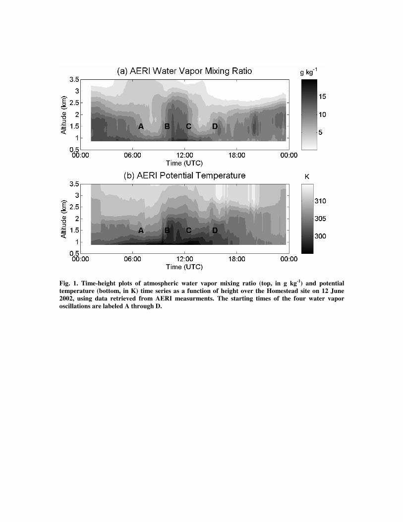
Fig. 1. Time-height plots of atmospheric water vapor mixing ratio (top, in g kg-1) and potential temperature (bottom, in K) time series as a function of height over the Homestead site on 12 June 2002, using data retrieved from AERI measurments. The starting times of the four water vapor oscillations are labeled A through D.

Fig. 2. Atmospheric soundings from (a) Dodge City, KS and (b) Amarillo, TX at 00 UTC on 12 June 2002. Source: UCAR JOSS IHOP_2002 catalog.

Fig. 3. GOES-8 infrared satellite imagery from 0802 UTC on 12 June 2002. The two MCSs propagating to the east through Kansas are labeled MCS1 and MCS2. IHOP_2002 locations of the Homestead site and S-Pol radar (not operational at this time) are labeled; other white dots indicate locations of Atmospheric Radiation Measurement (ARM) program observation stations. Image courtesy Space Science and Engineering Center (SSEC), University of Wisconsin – Madison.

Fig. 4. Radar reflectivity (in dBZ) image from the Dodge City, Kansas WSR-88D (KDDC) radar at 0816 UTC on 12 June 2002. Note the outflow boundary south of the KDDC radar site. The radar elevation angle was 0.4°; range rings are 50 km apart. The Homestead site is denoted by the dot in the Oklahoma panhandle. Data courtesy NCDC.

Fig. 5. Isochronal analysis from surface observations of the wind shift line, associated with the outflow boundary from MCS2 (Fig. 3), as it moved south and east across the Oklahoma panhandle from 08 UTC to 16 UTC on 12 June 2002.

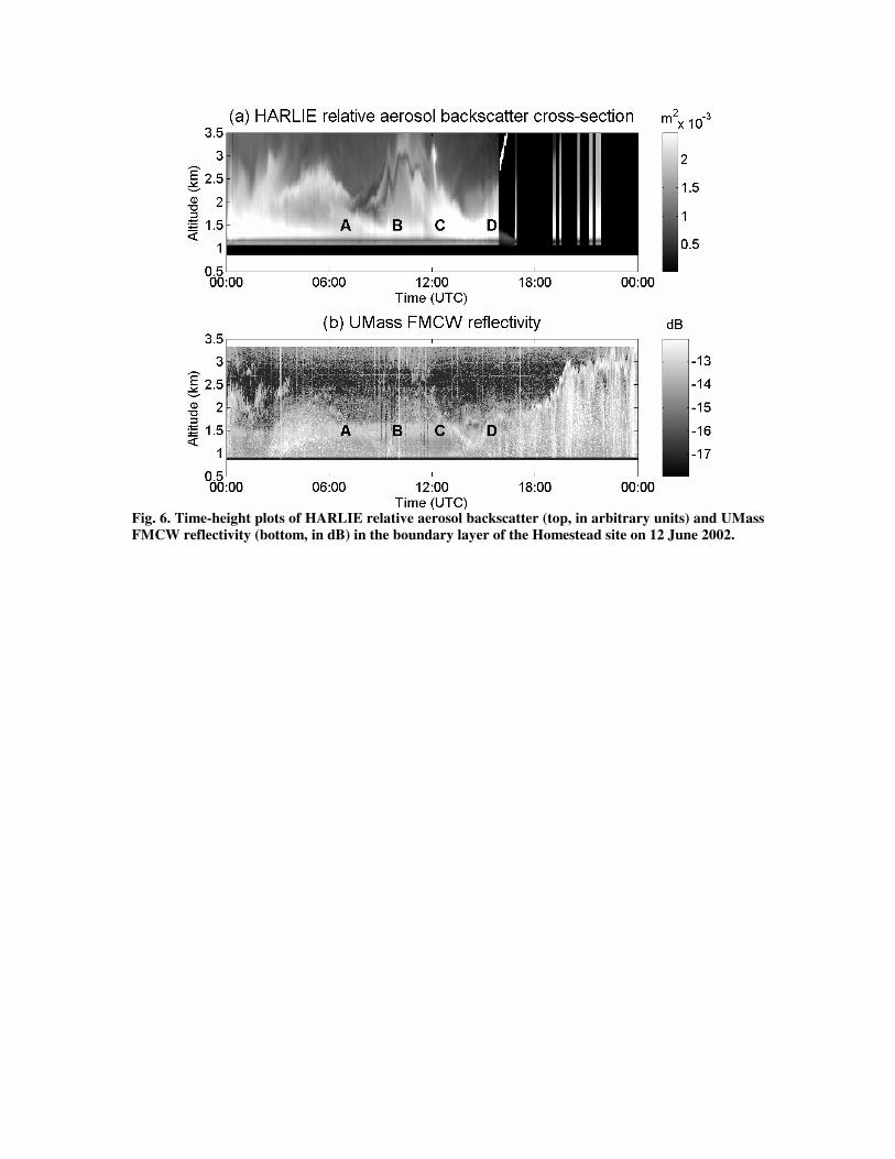
Fig. 6. Time-height plots of HARLIE relative aerosol backscatter (top, in arbitrary units) and UMass FMCW reflectivity (bottom, in dB) in the boundary layer of the Homestead site on 12 June 2002.

Fig. 7. Time-height plots of vertical velocity (in m s-1) over the Homestead site (a) as measured by the MAPR, and (b) as simulated by the ARPS (discussed later). Note that the gray shading scales differ between the two panels.

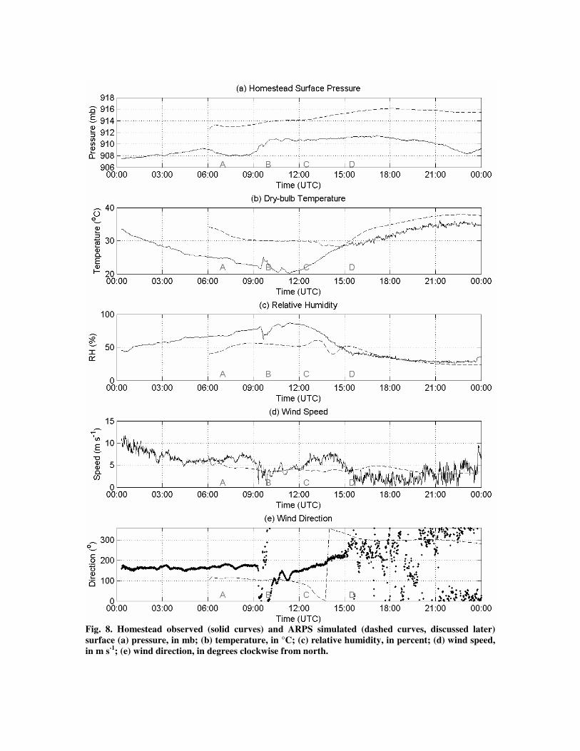
Fig. 8. Homestead observed (solid curves) and ARPS simulated (dashed curves, discussed later) surface (a) pressure, in mb; (b) temperature, in °C; (c) relative humidity, in percent; (d) wind speed, in m s-1; (e) wind direction, in degrees clockwise from north.

Fig. 9. The ARPS 9 km and 3 km resolution computational domains used in this study. Axes labels are in km from the lower left corner of the 9 km grid. The lines labeled A-B and C-D are the locations of cross-sections (discussed later).

Fig. 10. ARPS simulated surface potential temperature (K) fields on the 3 km grid at (a) 0900 UTC, (b) 1100 UTC, (c) 1300 UTC, and (d) 1500 UTC on 12 June 2002. The tip of the white arrowhead denotes the location of the IHOP_2002 Homestead site.

Fig. 11. Meridional cross-section (at the longitude of the Homestead site – line A-B in Fig. 9) of 9 km resolution ARPS simulated potential temperature field (in degrees K) at (a) 0900 UTC, (b) 1100 UTC, (c) 1300 UTC, and (d) 1500 UTC on 12 June 2002. The tip of the white arrowhead denotes the location of the IHOP_2002 Homestead site.

Fig. 12. Same as Fig. 11, but for the simulated water vapor mixing ratio field. Note the “wedge” of dry air (moving out of the page) in panels (b) through (d).

Fig. 13. Zonal cross-section (at the latitude of the Homestead site – line C-D in Fig. 9) of 9 km resolution ARPS simulated water vapor mixing ratio (in g kg-1) field at (a) 0900 UTC, (b) 1100 UTC, (c) 1300 UTC, and (d) 1500 UTC on 12 June 2002. The tip of the white arrowhead denotes the location of the IHOP_2002 Homestead site.

Fig. 14. Time series of (top) water vapor mixing ratio (in g kg-1) and (bottom) potential temperature, from ARPS simulation of the IHOP_2002 domain, at the grid point closest to the Homestead site.

Fig. 15. A conceptual model of the interaction between the bore associated with the outflow from MCS2 and the advancing dryline that produced the “wedge” of dry air depicted in the ARPS model simulations. The southward-moving bore waves, with their attendant regions of rising and sinking motion, generate “kinks” in the advancing dryline and, in some locations, decouple the dryline from the surface. One of the downward “kinks” in the dryline is shaped into the “wedge” (Fig. 13) by continued interaction with the bore.