SCHOOL EXPENDITURE LEAKAGE AND EFFICIENCY:

THE CASE OF THAI COMPULSORY EDUCATION

Jiradate Thasayaphan

A Dissertation Submitted in Partial

Fulfillment of the Requirements for the degree of

Doctor of Philosophy (Economics)

School of Development Economics

National Institute of Development Administration

2010

ABSTRACT

Title of Dissertation School Expenditure Leakage and Efficiency:

The Case of Thai Compulsory Education

Author Mr. Jiradate Thasayaphan

Degree Doctor of Philosophy (Economics)

Year 2010

The objectives of this study are to compute the leakage of public expenditure,

to diagnose weak institutional capacity, and to measure the efficiency and factors that

affect the performance of the schools in Thai compulsory education. The frame of

reference of the study is the school-based management framework, and the models

used to compute efficiency are Data Envelopment Analysis, Stochastic Frontier

Analysis, and Bayesian Stochastic Frontier Analysis model.

The samples were randomly drawn from small-sized, lower secondary schools

from Nakhonratchasema and Amnatcharoen provinces in Thailand. Two-stage

stratified cluster sampling was used as a sampling technique. The total number of

samples included in the study is 109; however, only 70 schools were included in the

econometric analysis.

The results of the study indicate that there exist leakages of public

expenditures, absence rate, and budget allocation delays in the sampled schools. The

average efficiency of schools was relatively high. However, leakage and weak

institutional capacity reduced the school efficiency, suggesting the role of government

intervention. In addition, the Bayesian Stochastic Frontier Analysis proved to be

superior for describing the characteristics of the best performing schools.

ACKNOWLEDGEMENTS

The author would like to express his sincere gratitude to committee

chairperson, Assistant Professor Dr. Dararatt Anantanasuwong, for her suggestions

regarding the topic of this dissertation. Her encouragement and guidance were the

crucial factors that made this dissertation successful. I also wish to extend thanks and

appreciation to all of the committee members, Associate Professor Dr. Sirilaksana

Khoman, Assistant Professor Dr. Santi Chaisrisawatsuk, Assistant Professor Dr. Anan

Wattanakulcharas, and Associate Professor Dr. Adis Israngura for their constructive

comments and suggestions.

Thanks are dedicated to the National Anti-Corruption Commission (NACC)

for their research grant, which supported my field survey in the northeast provinces so

that quality data and information could be obtained. Thanks also goes to the School of

Development Economics for their partial funding during the study as a research

assistant to Professor Dr.Nattapong Thongpakdee, which was a valuable time for me

to practice academic writing. Additionally, a short period of work at the Center of

Sufficiency Economy Study at the National Institute of Development Administration

(NIDA) also was the memorable time, especially for understanding numerous other

angles of economic thought.

Thanks also go to the librarians from the library and Information Center at

NIDA for their superb service in assisting Ph.D. students in all aspects, and to Dr.

Bruce Leeds for his reviewing and formal editing of the final stage of dissertation.

Special thanks are also extended to my parents, and my wife for their unconditional

love and support of everything throughout the writing process of this dissertation.

Finally, I would like to dedicate this dissertation to my beloved daughter, Ani, who

passed away before it was completed. She will remain in my mind and my heart

forever.

Jiradate Thasayaphan

April 2011

TABLE OF CONTENTS

Page

ABSTRACT iii

ACKNOWLEDGEMENTS iv

TABLE OF CONTENTS v

LIST OF TABLES viii

LIST OF FIGURES x

SYMBOLS AND ABBREVIATIONS xi

CHAPTER 1 INTRODUCTION 1

1.1 Introduction to the Study 1

1.2 Motivation of the Study 4

1.3 Objectives of the Study 8

1.4 Organization of the Study 8

CHAPTER 2 REVIEW OF THE LITERATURE 10

2.1 Literature Review on Leakage and 10

Weak Institutional Capacity

2.1.1 Leakage of Public Expenditure 11

2.1.2 Teacher Absenteeism 15

2.1.3 Budget Allocation Delay 17

2.2 Literature Review on Efficiency Measurement 19

2.2.1 Model Development 20

2.2.2 Previous Studies 36

CHAPTER 3 FRAME OF REFERENCE 42

3.1 The Service Delivery Framework 43

3.1.1 The Four Actors 44

3.1.2 The Market 46

vi

3.1.3 The “Sub-national Government” Model 48

3.1.4 School-Based Management 50

3.2 Student Achievement Production Function 52

3.2.1 Data Envelopment Analysis 53

3.2.2 Stochastic Frontier Analysis 54

3.2.3 Bayesian Stochastic Frontier Analysis 58

CHAPTER 4 RESEARCH METHODOLOGY 64

4.1 Public Expenditure Tracking Survey 64

and Quantitative Service Delivery Survey

4.2 Sample Selection and Data Collection 69

4.3 Variables for Production Function Estimation 73

4.4 Limitations of the Study 78

CHAPTER 5 ESTIMATION RESULTS 81

5.1 Leakage and Weak Institutional Capacity 81

5.1.1 Leakage of Estimation 83

5.1.2 Absence Rate 85

5.1.3 Subsidy and Compensation Delays 87

5.1.4 Correlation Study of Teacher Absent and Leakage 88

5.2 Efficiency: Education Production Function Estimation 92

5.2.1 Efficiency Distribution 92

5.2.2 “Jackknifing” with Outlier Observations 95

5.2.3 The Connection of Efficiency Scores to Variables: 96

A Tobit Model

5.2.4 Adjusted Efficiency Scores 107

5.2.5 Comparison of Technical Efficiency Estimation 111

CHAPTER 6 CONCLUSION AND POLICY RECOMMENDATION 117

6.1 Conclusion of the Study 117

6.2 Policy Recommendation 122

6.3 Implications for Future Research 124

vii

BIBLIOGRAPHY 125

APPENDICES 135

Appendix A The Jackknifing Procedure 136

Appendix B The Three-stage Approach 139

Appendix C Data on Thailand 149

Appendix D Research Instruments 150

BIOGRAPHY 265

LIST OF TABLES

Tables Page

2.1 Absence Rates by Country 16

4.1 Samples Included in the Study 71

4.2 Number of School Coverage by Type of Questionnaires 73

4.3 Description of Variables Used 75

5.1 Leakages of In-cash Subsidies, FY 2006-2007 84

5.2 Average Leakages of In-cash Subsidies, %, and Amount, 85

AY 2006

5.3 Absence Rate, Vacant Teacher Position in The School 86

and Shortage of Teacher Over One Semester (%), AY 2006

5.4 Subsidy and Compensation Delays 88

5.5 Logit and Probit Model: Marginal Effects of Variables 89

on Teacher Absence

5.6 OLS Estimates of the Correlation of ln Leakage of 91

Capitation Grants and ln Leakage of Fundamentally-needed

Funds, AY 2006

5.7 Efficiency Scores and Share of Efficient School 94

5.8 The Stability of DEA Results 95

5.9 Parameter of Tobit Models Explaining Inefficiency 97

5.10 Variables Descriptions Used in SFA 98

5.11 Parameter Estimate of Inefficiency Function 101

(Dependent variable = ln[Composite Scores], n = 70)

5.12 Parameters Estimate of the SFA, Specification II 103

5.13 Output Elasticity of Translog Function and Cross Elasticity of 105

Substitution

5.14 Average Efficiency, Minimum and Maximum Efficiency Scores 106

5.15 Initial and Final Efficiency Scores 109

ix

5.16 Efficiency Scores of BSFA 110

5.17 Average Efficiency Scores, DEA, SFA and BSFA 112

5.18 Frequency Distribution of Technical Efficiency 113

5.19 Difference between Sample Means for Paired Data 114

5.20 KRCC between Method 114

5.21 Common Characteristic of Efficient Schools 115

LIST OF FIGURES

Figures Page

2.1 Farrell’s Technical and Allocative Efficiency 21

2.2 Input- and Output-Orientated Technical Efficiency 24

2.3 Scale Efficiency 26

3.1 Five Features of the Accountability Relationship 43

3.2 Service Delivery Framework 44

3.3 The “Sub-national Government” model 49

3.4 School-Based Management and Four Accountability Relationships 51

4.1 Educational Administrations and Management Structure 67

4.2 Flow of Fund in Education Sector 68

5.1 The Flow of Funds in the Compulsory Educational Sector 82

SYMBOLS AND ABBREVIATIONS

Symbols Equivalence

AY Academic Year

BOG Board of Government

BOM Board of Management

BSFA Bayesian Stochastic Frontier Analysis

COLS Correct Ordinary Least Square

CRS Constant Returns to Scale

DEA Data Envelopment Analysis

DEO District Education Office

DMU Decision Making Unit

ESA Educational Service Area

FY Fiscal Year

KRCC Kendall Ranking Correlation Coefficient

LAO Local Administration Organization

LR Likelihood Ratio

ML Maximum Likelihood

MOE Ministry of Education

MOF Ministry of Finance

MOEYS Ministry of Education, Youth and Sport

NGO Non-Government Organization

NFT Non-Follow Through

NIETS The National Institute of Educational

Testing Service

OBEC Office of Basic Education Commission

OEC Office of the Education Council

OLS Ordinary Least Square

xii

PAP Priority Action Program

PEO Province Education Officer

PETS Public Expenditure Tracking Survey

PFT Program Follow Through

PISA Program for International Student

Assessment

PT Provincial Treasuries

PTA Parent-Teacher Association

QSDS Quantitative Service Delivery Survey

SBM School-Based Management

SE Scale Efficiency, Standard Error

SFA Stochastic Frontier Analysis

SFR Stochastic Frontier Regression

TE Technical Efficiency

TIMSS Trends in International Mathematics and

Science Study

TOPS Technically Optmal Productive Scale

VRS Variable Returns to Scale

CHAPTER 1

INTRODUCTION

“Economics is a study of cause-and-effect relationships in an economy. It’s

purpose is to discern the consequences of various ways of allocating resources which

have alternative use.”

Thomas Sowell (2000: 39)

1.1 Introduction to the Study

The role of human capital in economic development has drawn the attention

of economists, as education is viewed as key for economic growth (Mankiw, Romer,

and Weil, 1992: 433). Thailand has recognized the importance of education; by the

1800s, King Chulalongkorn, the fifth king of the Chakri Dynasty, had initiated an

education reform. By 1911, 29% of the male age group was receiving education. By

the year 1935, modern education had been extended to every community of the

Kingdom (Wyatt, 1969: 373). Fry (2002: 22) has indicated the major areas of

educational problems in Thailand: fragmented human resources development and

education, the highly centralized bureaucracy of the Thai educational budget,

traditional teacher-centered learning modes, neglect of science and related research

and development, and persistent equity and access issues. By the late 1990s, with the

drafting of the National Education Act (1999), there was a major overhaul of the

education system.

2

Thailand launched an educational reform intended to address problems

relating to equity, quality, and financing. Thailand has made significant progress in

addressing the equity issue. The primary education completion rate in 2000 and 2007

was 96% and 101%, respectively, and the gross secondary education enrollment rate

in year 2000 and 2007 was 67% and 83%, respectively (World Bank, 2009:

204).However, Atagi (2002: 23) has indicated that Thailand has not obtained an

adequate return for its investments in education. Basically, she argued that despite

Thailand’s relatively high percent of government budget spent annually on education,

Thailand lags behind internationally on many major indicators of educational quality.

The World Bank (2007: 74-77) has reported that public expenditure on

education as a percent of total government expenditure for Thailand, the Republic of

Korea, Hong Kong, Japan, and Malaysia was 28%, 15%, 23%, 11%, and 28%,

respectively. However, the Trends in International Mathematics and Science Study

(TIMSS), which reported the comparative test scores of grade eight students regarding

mathematics and science literacy of grade eight students were only 55% (Martin,

Mullis and Foy, 2008a: 35), and 58% (Martin, Mullis and Foy, 2008b: 34) of the total

scores , respectively. These results are not only below the scores of countries in Asia,

such as the Republic of Korea, Hong Kong, and Japan, but also below the

participating Southeast Asian countries, such as Singapore and Malaysia. Regarding

the Program for International Student Assessment (PISA), which tested the students’

literacy in compulsory education (for 15 year old students), which measures the

“yield” of educational systems, the score of students from Thailand were only 41%

and 42% of total scores for mathematics and the sciences (OECD, 2010: 8),

respectively.

Public expenditure on education is the major part of the national budget in

most of the countries. Over 37,000 educational institutions with nearly 20 million

students in the Thai education system enroll from their early years to higher

education, encompassing both formal and non-formal education. The education

budget set aside for Thai education constitutes about 4% of the gross domestic

product, or about 24%, and 22% of the national budget in 2004 and 2008,

respectively. However, the achievement scores of grade 9 students in 2008 on the

national test for mathematics and science literacy were only 32% and 39%,

3

respectively. Further, in 2009, the mathematics and sciences scores were only 26%

and 29%, respectively (NIETS, 2011: 1).

The education provided by the government is equivalent to the provision of

any other public good. From the economic point of view, there are reasons to ensure

positive production whenever there exist externalities from individual choice and

institutional factors. Public good is characterized by underproduction in a market

solution, because private demand would fall short of optimal provision. This may

offer a rationale for the diffusion of compulsory and freely provided education in all

countries.

Woessman (2000: 79-80) has argued that improving the institutional

environments of education is a crucial factor for ensuring efficient use of resources. This

productivity is determined by the behavior of the people who act in the educational

process, and student performance is influenced by the productivity of resources used in

schools. These people respond to incentives and their incentives are set by the

institutional environments of the system. Coase (1984: 230) stressed that “the choice in

economic policy is a choice of institutions.”

As pointed out by Glewwe and Kremer (2005: 50-51), schools in developing

countries face significant institutional environment problems; distortions in education

budgets often result in inefficient allocation and spending of funds, weak teacher

incentives lead to problems such as high rates of teacher absenteeism, and curricula

are often inappropriately matched with the level of the typical student. Governance

reforms and allowing school choice appear to hold more promise than simply

providing monetary incentives to teachers based on test scores. However, some

observers have argued that these schools may need more resources, while others

emphasize the weaknesses of the school systems and the need for reform. These two

views both may be true—some types of spending will have low marginal product

while others will have high marginal product. Hence, carefully-targeted investment in

education administration can be extremely productive in such settings.

4

1.2 Motivation of the Study

The per head expenditure (capitation grants) for students has been generally

considered the investment of the government in basic education, suggesting that it is

required that resources have to be allocated to schools efficiently, and the schools

have to utilized these resources as productively as possible. However, Worthington

(2001: 245-246) has argued that measuring educational efficiency by using the

production function, where outputs are a proxy of standard test scores and inputs are a

proxy of capitation grants, could be questioned. The first question concerns the

validity of the educational production function framework itself. It is argued that

many empirical studies are ad hoc in their selection of methodology and, in particular,

selection of inputs and outputs variables are at odds with the production function

approach itself. The second centers on the possibility that public policy does not have

any measurable impact on educational outcomes. This suggests that innate ability,

combined with the influence of socioeconomic background, may dominate the

educational production process (Deller and Rudnick, 1993 quoted in Worthington,

2001: 246). Mayston (1996: 141) has argued that the lack of a positive relationship

between educational outcomes and educational expenditure is the result of schools

balancing off demand-side considerations of “willingness to pay” for additional

educational attainment against supply-side factors related to the genuine underlying

production function. In addition, the educational production function approach relies

on an assumption of efficiency. It is assumed that all institutions in a given context are

able to transform educational inputs into academic outputs at the same rate. If this is

not the case, then the empirical application of the conceptual model may collapse

(Hanushek, 1986 quoted in Worthington, 2001: 246).

A large number of empirical studies to date have already considered the

possibility that inefficiency exists in education. These studies have used a variety of

empirical techniques to identify “efficient” educational institutions and have

compared them with “inefficient” institutions. This work is obviously important

because, in most developed economies, emphasis has been given to issues of

accountability, value for money, and cost effectiveness in education. The

5

measurement of organizational efficiency is thus recognized as an essential part of the

implementation, monitoring, and evaluation of these public-sector reforms

(Worthington, 2001: 246). “Technical efficiency” refers to the use of production

resources to produce goods and services in the most technologically efficient manner.

It follows that a strong assumption held in this type of analysis is that technical

relationships are of central importance in the educational process. If such relationships

exist and can be quantified, education policy can be constructed so as to maximize

conceptual outcome. Hence, much of the empirical research in this area is focused on

identifying these technical relationships.

The economic theory of production function indicates that given an amount

of inputs, the production function defining the Pareto efficient given set of outputs is

that it is not possible to increase the quantity of any outputs without decreasing the

quantity of any other outputs; in other words, for given outputs, it is not possible to

decrease the quantity of any inputs without increasing the quantity of any other inputs.

Efficient decision making units (DMUs) will produce goods and services at the

frontier of production technology, since the deviation from the frontier means

inefficiency. Following this logic, the empirical study of efficiency difference

involves determining the production frontier and measuring the distance to the

frontier of these individual observations.

Educational resources are allocated for a particular purpose within legally-

defined institutional arrangements; however, information on actual spending at the

provider is seldom available, especially in developing countries. Public service

provision could be affected by institutional inefficiencies, such as leakage of public

resources, weak institutional capacity, and inadequate incentives. In this study, weak

institutional capacity includes only absent rate and budget delays. Ablo and Reinikka

(1998: 31) showed that there are leakages of public expenditure at the school level,

and capitation grants do not reach frontline service providers. Consequently, the

effectiveness of services is affected by such institutional inefficiencies.

This paper argues that budgetary allocations could be misleading in

explaining educational outcomes. Making policy decisions in a weak institutional

capacity requires sufficient information. Dixit, 1996 quoted in Ablo and Reinikka,

1998: 1 argued that governments are viewed as benevolent single agents, behaving in

6

the same way everywhere in the world, and policy-making is a technical problem

rather than a political process that varies between countries. This normative view of

government has led to the general practice of measuring public expenditure, both

capital and recurrent. This study presents a detailed diagnosis of the problems in

practice, using empirical evidence. The study argues that the leakage of public

expenditure will have the effects to the education outcomes.

The motivation for this study was the observation that since 1999, public

spending on basic services had substantially increased in Thailand, while officially-

reported outcome remained stagnant. The most obvious disparity in outcome

indicators was observed in compulsory academic achievement (as described in 1.1).

Despite the fact that budgetary allocations for education increased over time, there

was hardly any increase in the reported student achievement. To study this issue, two

types of research instruments were invented, the Public Expenditure Tracking Survey

(PETS) and the Quantitative Service Delivery Survey (QSDS). A PETS can quantify

leakage, track the flow of resources through strata of bureaucratic structure, and

determine how much of the originally-allocated resources reach each level. The

instrument can also be used to evaluate impediments to the reverse flow of

information in order to account for actual expenditures (Reinikka and Smith, 2004:

33-34). A QSDS has the primary aim of examining the efficiency of public spending,

dissipation of resources, incentives, and various dimensions of service delivery in

providers’ organizations, especially at the front line. It collects data on inputs, outputs,

quality, pricing, oversight, and so forth. The facility or frontline service provider is

typically the main unit of observation (Reinikka and Smith, 2004: 43).

The World Bank (2003: 47) created the analytical framework, school-based

management (SBM), which is applied to this study. In a certain SBM framework, the

accountability of school principals is upward to the ministry of education, which

holds them responsible for providing services to students, who in turn have put

politicians in power. In most cases of SBM, the management changes under reforms

process. The parents themselves become part of the school management. Parents have

the authority to make certain decisions that affect the students that are attending the

school. The quality of public service is difficult to monitor; this is called a

“monitoring problem,” since locally-produced services such as basic education have

7

some characteristics that make it particularly difficult to structure the accountability

relationship. In this case, the basic education service is the so-called “transaction-

intensive,” and this transaction requires discretionary judgments in the service

delivery, because it is difficult to know whether the provider has performed well. In

fact, it is difficult to monitor the millions of daily interactions of teachers with

students. As a result, rigid, script rules would not provide enough latitude in the case

of multi-principals and multi-tasks, where public servants “serve many masters.” The

SBM framework then is introduced whereby the school administrator, whether the

head teacher alone or a committee of parents and teachers, acts as the “accountable

entity.” Problems such as leakage of funds and absenteeism can result from a failure

in any one of the key relationships of accountability. Public funds may be captured to

fund the political machinery; beneficiaries may be kept in the dark about their

entitlements. Without such strong relationships, there may be no incentives to monitor

that teachers are in the classroom (Reinikka and Smith, 2004: 30).

By incorporating leakage and institutional capacity information with its

inputs-outputs relationship, the literature on production frontiers provides a suitable

method to calculate the technical efficiencies of service providers. This empirical

study then uses the non-parametric and parametric method. The non-parametric

method is known as data envelopment analysis (DEA), and the parametric method

includes stochastic frontier analysis (SFA) and Bayesian stochastic frontier analysis

(BSFA). The results and policy prescriptions will be explained within the SBM

framework. This study will also compare the result calculations from each method,

and estimate the firm-specific efficiency scores of the samples schools.

The hypothesis of the study is that the success of actual service delivery

(outputs) is worse than education investment (inputs), implied public funds do not

reach the intended facilities as expected. Furthermore, even if? the school receives

that budget, the schools weak in institutional capacity prevent schools to use this

efficiently, and hence outcomes cannot improve. The reasons for facilities not

receiving the public funds could range from priorities at various levels of government

to misuse of public funds. As adequate public accounts are not available in public

officials, including Thailand, a micro-survey of schools had to be carried out to

collect actual data. A public expenditure tracking survey (PETS) was conducted to

8

compare budget allocations with actual spending through the layers of bureaucratic

structure, and a quantitative service delivery survey (QSDS) as conducted to collect

various data at providers including a numerous variables related to institutional

capacity. Although this study does not attempt a comprehensive analysis of the

determinants of educational sector efficacy, the government’s capacity to translate

public expenditure allocation into actual spending at the facility level is a proxy for it.

The study also attempts to incorporate the institutional factors in the econometric

model as a case study to measure the efficacy of public sector.

1.3 Objectives of the Study

The specific objectives of this study are as follows:

1. To quantify the leakage of public funds proxy by capitation grants and

fundamentally-needed funds.

2. To diagnose weak school institutional capacity, teacher absenteeism, and

budgetary allocation delay.

3. To measure the school’s technical efficiency and to explain the factors

that influence school efficiency empirically based on the survey.

4. To compare the school’s technical efficiency empirically, based on each

estimation technique.

1.4 Organization of the Study

This study is organized into six chapters. Chapter 1 presents the introduction.

Chapter 2 provides a review of the literature. Chapter 3 provides the frame of

reference employed in the study. Chapter 4 presents the research methodology.

Chapters 5 provide an estimation of the leakage of public expenditure, and diagnoses

weak institutional capacity in the school. Chapters 6 provide policy recommendations

9

within the proposed frame of reference, conclude the study, and suggest implications

for future research.

CHAPTER 2

REVIEW OF THE LITERATURE

“The consequences for human welfare involved in questions like these [about

economic growth] are simply staggering: Once one starts to think about them, it is

hard to think about anything else.”

Robert E. Lucas, Jr. (1988: 5)

This chapter provides the context for understanding how leakage of public

expenditure and weak school institutional capacity may have an effect on academic

achievement in Thai compulsory education. The scope of this literature review will be

limited to the leakage of public expenditure, evidence of weak school institutional

capacity in the service delivery system, and efficiency measurement concepts.

2.1 Literature Review on Leakage and Weak Institutional Capacity

Government resources earmarked for particular uses within legally-defined

institutional frameworks, often passing through a few layers of government

bureaucratic structure down to service facilities, are charged with the accountability of

exercising spending.

11

Public service provision could be affected by institutional inefficiencies such

as leakage of public resources, weak institutional capacity, and inadequate incentives.

Indeed, even if spending is officially allocated to services that target the poor, funds

may not necessarily reach frontline service providers, and the effectiveness of services

may consequently be affected by such institutional inefficiencies (World Bank, 2003

quoted in Gauthier, 2006: 1). The following section comprises a literature review on

the idea of the leakage of public expenditure.

2.1.1 Leakage of Public Expenditure

Certain patterns in resource leakage levels have tended to emerge from

previous PETS findings, in particular, in terms of: (i) rule-based versus discretionary

expenditure; (ii) wage versus non-wage expenditure; (iii) level of government; and

(iv) in-kind versus cash transfers. As emphasized by Das et al. (quote in Gauthier,

2006: 33), the level of discretion exercised on resource allocation could influence

leakage levels. Greater discretionary power granted to particular administrative units,

combined with weak supervision and improper incentives, could lead to large fund

leakage. Indeed, differences in leakage levels have been observed between funds

allocated through fixed-rule and those that are at the discretion of public officials or

politicians. Since rule-based funding is clearly defined according to a simple

allocation rule, leakage of funds is more difficult compared with discretionary funds,

which are bound by specific allocation rule. Wages are also often paid directly by the

central government to individual workers at the service provider, without going

through the administrative apparatus. Alternatively, when wages transit through the

administrative structure, they are generally paid by local authorities directly to

workers, thus with the same incentives at the recipient level for ensuring full transfer.

In the case of non-wage expenditures, local officials and politicians could take

advantage of their information advantage to reduce disbursement or provide few non-

wage supplies to schools, knowing it would attract little attention (Reinikka and

Svensson, 2004: 38). Leakage is associated with different institutional structures,

characterized by various information asymmetry problems among parties, coupled

12

with discretionary power and weak enforceability. Leakage has also been shown to be

more pronounced in the case of in-kind transfers compared with in-cash transfers.

Although school officials and parents know that they are entitled to some funding

from the district level, because resources reaching the schools are predominantly in-

kind without any indication of monetary values, school communities seldom know the

value of the in-kind support they receive, which greatly reduces accountability.

Gauthier (2006: 27-31) indicates that for the first PETS in Uganda done in

the education sector tracking capitation, on average during 1991-1995 the leakage rate

was about 87%, due to asymmetric information that adversely effected on the flows of

funds to frontline providers. Leakage appears principally at the district level of

education, and resources disappeared for private gains or were used by district

officials for expenditures unrelated to education administration. The finding also

revealed that there was a large variation in leakage across schools—larger schools

appeared to receive a larger share of the intended funds, schools with children of

better-off parents experienced a lower degree of leakage, and schools with a higher

share of unqualified teachers experienced more leakage. According to a follow-up

tracking carried out in 1999 and 2000, the leakage was about 18%. The improvement

was associated with the school obtaining better information about school entitlements

through radio and newspaper campaigns. The information campaign was estimated to

account for about 75% of the improvement in leakage. According to a 1999 survey in

education carried out in Zambia, non-wage expenditure leakage was estimated at

57%, appearing at the district level. Further, according to a study in Ghana in 2000

tracking non-wage expenditure and wage in education, leakage was estimated at about

50% and 20%, respectively. A large proportion of the leakage seemed to occur

between the central government and district office during the procurement process,

when public expenditure was translated into in-kind transfers.

According to a 2001 survey in Zambia, regarding track-fixed school grants

and a discretionary non-wage grant program for basic education, the result showed

that the leakage rate was 10% for fixed-rule grants and 76% for discretionary non-

wage expenditure. Rule-based funds were progressive, as greater per-pupil funding

was observed in poorer schools and discretionary disbursement was higher at the rich

schools in rural areas. Overall, public funds were regressive; 30% of resources were

13

allocated to richer schools compared with typical schools. The finding concludes that

a disbursement delay may be a factor in the leakage of rule-bases funds. For

discretionary funds, only a few schools that received large amounts of funds had

greater bargaining power with public officials.

In Kenya, according to a 2004 survey in the education sector, 80% of schools

did not receive their entitled amount of bursary funds and total leakage was estimated

at 35.8%. There was evidence that some schools received an allocation larger than

that to which they were entitled, and that funds were diverted for personal gains. The

study argued that the cause of the leakage stemmed from high discretion on the part of

the head teacher in financial management, with minimal influence of the parent-

teacher association (PTA) or school’s board of government (BOG). Lack of

information at the school level leads to non-accountability of public resources, and

poor records maintained by schools and lack of proper audits.

Fundamental and generic problems noted in the survey concerned

information asymmetry through the service providers’ supply chain. In most countries

examined, there was a crucial lack of information at various levels in the public-

organizational structure, in particular, at the central level, regarding resource use and

transfers through the supply chain. Information problems are acute at the lower levels

of the hierarchy, as decentralized administrative units are generally not aware of the

budgetary resources to which they are entitled. The information gap and retention of

information at the central level in several of the countries surveyed reinforces the

issue of moral hazard problems (Gauthier, 2006: 35-36). In Cambodia, a 2005 survey

of primary education reported a funds gap in priority action program 2.1 (PAP 2.1),

had trial in all of the years except in 2001. Except for 2000, there was significant

variation across provinces and within provinces. The gap went from 3.1% in 2000 to

23.5% in 2001, and then down again to 6.3% in 2002. Within variation, total funding

gaps were 94%, 69%, and 50% in 2000, 2001, and 2002, respectively (World Bank,

2005a: 20).

Because of these problems, as noted by Ablo and Reinikka (1998: 30-31),

public expenditure for social spending may have little impact on population status

because expenditure may not translate into improved service. Budget allocations may

not matter when institutions or their population control are weak. Therefore, despite a

14

paucity of data on what public funds are actually used for, public expenditure analysts

must find other ways to go beyond them. In sum, official public resources may not

adequately measure the availability or effectiveness of services in a context where

mismanagement could be a principal issue.

In most countries, the government assumes that local government has more

information on citizens’ needs. Governments have put forward an agenda on

decentralization, which may include fiscal policy and administration. A few tracking

surveys have been used to examine the impact of decentralization on the social

sector’s resource allocation. Ablo and Reinikka (1998: 22), for example, reported that

decentralization appeared to have led to a slight deterioration in the flow of funds to

schools. Local governments that possessed decentralized responsibilities for longer

periods of time presented greater fund capture compared with more recently

decentralized local government, and fewer transfers to schools. Das et al. (2004: 34)

also incorporated the question of decentralization in the schools sampled in Zambia.

They presented the negative effect on funds flow to service providers. The surveys

indicate that decentralization improved the flow of funds by decreasing spending at

the provincial level, and somewhat reduced the allocation of funds to schools. Indeed,

decentralized provinces presented greater levels of funds capture than centralized

provinces, and there is no evidence that increased funding to districts in decentralized

provinces is passed on to schools. Overall, approximately 11% to 33% of total

funding in the system of rule-based and discretionary funding reaches schools.

Schools in centralized provinces receive around 30 percent of total funds in the

system compared with about 25 percent for schools in decentralized provinces.

In 2005, Cambodia PETS (World Bank, 2005a: 21-23), the Ministry of

Education, and Youth and Sport (MOEYS) decided how to distribute its budget to the

provinces. The Province Education Office (PEOs) decided how to allocate cash to the

different PAP activities. PEOs have discretion over the allocation of PAP 2.1 funds to

the District Education Office (DEOs) and schools. This may help to explain the

funding gap variation within provinces. Overall, the leakage of PAP 2.1 funds, as

measured by facilitation fees, was small relative to total disbursement. Added

together, the 1.5% paid to DEOs by schools, the 0.5% paid by DEOs to PEOs, and

PEOs to Provincial Treasuries (PTs) yield a funds gap at 2% of facilitation fees out of

15

total disbursement. However, most of the PAP 2.1 funding gaps can be explained by

differences between budget allocations and disbursements to provinces. The

difference between what schools are entitled to and what they receive can be divided

into the difference between entitlements and disbursements to provinces, and the

difference between the disbursements and the funds actually received by schools. The

results indicate that most of the funding gaps are due to gaps in budget execution. In

terms of equity and impact on school environment, the analysis indicated that

allocation of funds was pro-poor, while the timing of disbursements tended to be

wealth neutral.

2.1.2 Teacher Absenteeism

Another question that has been studied, for which interesting results were

obtained, is the problem of absenteeism among school workers. QSDS have been used

to study absenteeism among workers. Table 1 presents the findings on absence rate

from a multi-country study (Chaudhury et al., 2006; Rogers et al., 2004; Chaudhury

and Hammer, 2004 quoted in Gauthier and Reinikka, 2007: 35-36). The study

reported the results from surveys, visits to primary schools in Bangladesh, Ecuador,

India, Indonesia, Peru and Uganda, and collected data on whether they found teachers

in the schools. Averaging across the countries, about 19% of teachers were absent.

The survey focused on whether providers were present in their facilities; however,

many providers that were at their school were not working, and even these findings

may be an underestimation The study analysed the high absence rates across

countries, investigated the correlates, efficiency, and political economy of teacher

absence, and considered implications for policy.

16

Table 2.1 Absence Rates by Country (%)

Country Primary schools

Bangladesh 16

Ecuador 14

India 25

Indonesia 19

Papua New Guinea 15

Peru 11

Uganda 27

Zambia 17

Source: Gauthier and Reinikka, 2007: 36.

The impact of teacher absence is evidenced in Das et al. (2005a: 20), who

used a household optimization framework to identify the impact of teacher-level

shocks on students’ learning gains. The data from Zambia showed that shocks to

teacher inputs had a substantial effect on student learning. Shocks associated with a

5% increase in the teacher’s absence rate resulted in a decline in learning of 3.7%

(English) and 4% (mathematics) of the average gains across the two years. Teachers

worked harder to compensate for such absences but children with a frequently absent

teacher may fail to improve in their test scores. The findings suggest that programs to

allocate substitute teachers could significantly improve education outcomes in such an

uncertain environment.

A few studies have quantified the share of job captured; that is, teachers that

continue to receive wages but that are no longer in government service or who have

been included in the payroll without ever being in service. In Africa, figures were

higher at 20% in Uganda in 1993; in Honduras, a combination of PETS and QSDS

was used to diagnose moral hazard with respect to frontline education staff (Reinikka

and Svensson, 2003: 4). The Honduras study showed that even when wages and non-

wage funds reach frontline providers, some staff behaviors and incentives in public

service have an adverse effect on service delivery, particularly regarding employees’

17

absenteeism and job capture. The major problem was the migration from posts due to

capture by employees. In the system of staffing in Honduras education, where posts

are assigned by the central ministry, frontline staffs have an incentive to lobby for

having their posts transferred to attractive locations. The PETS and QSDS in

Honduras compared staff assignments between the official record and real allocations,

and determined the degree of attendance at work. The survey used central government

information sources and a representative sample of education frontline facilities.

Central government payroll data indicated each employee’s workplace. The unit of

analysis was both the facility and the staff members. In this study, the authors

included all levels of the two sectors, from the ministry to the service facility level.

They reported that 5% of teachers on the payroll were found to be ghosts; and stiff

migration was highest among non-teaching staff and secondary teachers. Moreover,

multiple jobs in education were twice as prevalent, as 23% of all teachers held two or

more jobs, and 40% of the educational staff worked in administrative jobs.

2.1.3 Budget Allocation Delay

PETS and QSDS have also shed light on the question of delays and

bottlenecks in the allocation of resources through public administrations (e.g. wages,

allowances, financing, materials, and equipment). These issues could have important

effects on the quality of services, staff morale, and the capacity of providers to deliver

services. Gauthier (2006: 47-49) has presented estimates on delays in various

countries for certain types of items and inputs. According to the first PETS from

Uganda in 1996, anecdotal evidence showed that teachers’ wages suffered from

delays; however, payments reached schools relatively well. According to the Tanzania

2001 PETS, there were delays in non-wage disbursement and processing, ranging

from 6 to 42 days at the treasury. They observed delays in all districts by which

councils were not made transfers. Wage disbursement was rarely delayed, and delays

were reported to be worse for non-wage expenditures versus wages, particularly in

rural areas. This is evidence of a link to the cash budgeting system, and the fact that

wages are prioritized in the budget.

18

Concerning Rwanda surveys, the two PETS in 2000 for education reported

delays in budget execution at the central government level and considerable delays in

transfers between regions and districts. Delays were largely attributed to the

application of the cash budgeting system in the Ministry of Finance (MOF), and cash

constraints of the government. Regarding the 2004 Rwanda PETS for education, in

particular, delays were observed in the payment of capitation grants to schools.

Thirteen percent of teachers did not receive their salaries regularly and 82% had

salary arrears. Concerning the students surveyed, 43% of them reported irregularities

in the payment of the Education Support Fund program. It should be noted that only

47% of teachers knew the amount of their salary arrears. The major cause of delay in

Rwanda stemmed from the teachers not receiving detailed pay slips on salaries. They

lacked information about their exact salary at the source.

The 2001 PETS in the Zambian education sector reported that 5% of

teachers’ wages incurred delays, about 20 percent of teachers’ hardship allowances

incurred delays, and double class allowances were 6 month overdue for more than

75% of recipients. Well-defined allowances (hardship and responsibilities) tend to be

paid on time; however, less well-defined allowances suffer important delays. Delays

in the case of double class allowances and student trainees in part are due to lags in

payroll updating. In Namibia 2003 survey, delays in the supply of books at the school

level stemmed from mismatch between MOE textbooks catalogue and available books

at the facilities.

Delays in received public expenditure were evidenced in the Cambodia 2005

PETS (World Bank, 2005: 33) and were due to technical problems at the central level;

the 2002 PAP budget year had the longest delays as well as the most thinly-spread

disbursements. The MOEYS experienced difficulties in securing the release of PAP

funds in 2002 due to delays in procurement procedures, and difficulties in establishing

decentralized management at the provincial and district levels. The 2002 PAP funds

for education were delayed until a regulatory framework for proposed spending was

agreed upon in October 2002, which set the per-school and capitation allocation and

guidelines on the use of school operating budgets. These delays led to school

inefficiency in the use of funds by making it difficult for schools to plan ahead, and to

implement existing schools plans. As a result of uncertainty about the following

19

year’s funding, schools often used the current year funds to purchase equipment for

the following year instead of using the money for the current year’s uses. Thus,

unpredictability of funds leads to misuse of funds. The study also found problems

with the thinly-spread distribution of funds and increased transaction costs. Having

too many small volume disbursements increases transaction costs in transferring funds

from the PEO to the DEO and from the DEO to the school, as these transactions

involve physical visits to pick up the money. These costs include: (i) transportation

costs, particularly for schools located in remote areas; (ii) ―mission allowances.‖

which might include food and accommodations for the person(s) coming to pick up

the money; and (iii) ―facilitation fees‖ that need to be paid out. Thus, the total amount

paid for facilitation during the year increased with the number of transactions.

In sum, this section has reviewed the previous findings using PETS and

QSDS, and both tools can be used for analyzing the efficiency in public expenditure

spending. The following section is a brief literature review of the efficiency

measurement concept.

2.2 Literature Review on Efficiency Measurement

Economists have developed three main measures of efficiency. First,

―technical efficiency‖ refers to the use of productive resources in the most

technologically-efficient manner. This implies the maximum possible output from the

given set of inputs. In the context of education production, technical efficiency refers

to the physical relationship between the resources used (say capital, labor and

equipment) and educational outcomes, which may either be defined in terms of

intermediate outputs (generally, standardized test scores) or a final education outcome

(such as graduates’ employment rates, starting salaries, or acceptance rates into higher

education). The second, ―allocative efficiency,‖ reflects the ability of firms to use

inputs in an optimal manner, given their respective prices and technology. The

combination of technical and allocative efficiency determines the degree of

―productive (economic) efficiency.‖ Thus, if an organization uses its resource

20

complete allocatively and technically efficiency, then it can be said to have achieved

total economic efficiency. If there is either technical or allocative inefficiency, then

the organization will operate with less than total economic efficiency. The next

section presents an econometric model that attempts to measure technical efficiency.

2.2.1 Model Development

The basis for frontier analysis was offered by Koopmans (1951 quoted in

Fried, Lovell and Schmidt: 2008: 20), who provided a formal definition of technical

efficiency; a producer is technically efficient if an increase in any output requires a

reduction in at least one other output or an increase in at least one input, and if a

reduction in any input requires an increase in at least one other input or a reduction in

at least one output. Thus, a technically-inefficient producer could produce the same

outputs with less of at least one input or could use the same inputs to produce more of

at least one output. Debreu (1951: 275-291) and Farrell (1957: 254-260) introduced a

measure of technical efficiency. With an input-conserving orientation, their measure

is defined as (one minus) the maximum equiproportionate (i.e. radial) reduction in all

inputs that is feasible with given technology and outputs. With an output-augmenting

orientation, their measure can be defined as the maximum radial expansion in all

outputs that is feasible with given technology and inputs. In both orientations, a value

of unity indicates technical efficiency because no radial adjustment is feasible, and a

value different from unity indicates the severity of technical inefficiency.

Farrell’s (1957: 254-260) argument is presented in Figure 2.1, where two

inputs, x1 and x2, are utilized to produce a single output, y, so that the production

frontier is y = f(x1 , x2). If constant returns to scale are assumed, then 1 = f(x1/y,

x2/y). The isoquant of the fully-efficient firm SS permits the measurement of

technical efficiency. Now, for a given organization using quantities of inputs (x1*,

x2*) defined by point P (x1*/y, x2*/y) to produce a unit of output y*, the level of

technical efficiency may be defined as the ratio OQ/OP. This ratio measures the

proportion of (x1*, x2*) actually necessary to produce y*.

21

Figure 2.1 Farrell’s Technical and Allocative Efficiency

Thus, 1 – OQ/OP, the technical inefficiency of the organization, measures

the proportion by which (x1*, x2*) could be reduced (holding the input ratio x1/x2

constant) without reducing output. It accordingly measures the possible reduction in

the cost of producing y*. Furthermore, given constant returns to scale, it also roughly

estimates the proportion by which output could be increased, holding (x1*, x2*)

constant. Point Q, on the contrary, is technically efficient since it already lies on the

efficient isoquant.

These efficiency measures assume that the production function of the fully-

efficient firm is known; in application however, the efficient isoquant must be

estimated using the sampled data. The Farrell approach estimates the ―relative best

practice‖ rather than average technology. The estimation technique can be broadly

categorized into two branches: econometric approaches and the programming

approach.

First, the econometric approach specifies the production function, and it

normally recognizes that deviation away from this given technology (as measured by

the error term) is composed of two parts, one representing randomness (or statistical

noise) and the other inefficiency. The usual assumption with the two-component error

structure is that the inefficiencies follow an asymmetric half-normal distribution and

the random errors are normally distributed. The random error term is generally

x2/y

x1/y

P(x1*/y, x2*/y)

S

Q

Q R

A

0 A

S

22

thought to encompass all events outside the control of the firm, including both

uncontrollable factors directly concerned with the ―actual‖ production function (such

as differences in operating environments) and econometric errors (such as

misspecification of the production function and measurement error). This type of

reasoning has primarily led to the development of the ―stochastic frontier approach,‖

which seeks to take these external factors into account when estimating the efficiency

of real-world firms.

Second, the mathematical programming approach which seeks to evaluate

the efficiency of a firm relative to other firms in the same production technology

setting. The most commonly-employed version of this approach is linear

programming, referred to as ―data envelopment analysis (DEA).‖ DEA essentially

calculates the technical efficiency of a given firm relative to the performance of other

firms producing the same good or service, rather than against an idealized standard of

performance. DEA is a non-stochastic method and it assumes that all deviations from

the frontier are the result of inefficiency.

In order to relate the Debreu-Farrell measures to the Koopmans definition,

let producers use inputs, 1( ,..., )N Nx x x R , to produce outputs, denoted by

1( ,..., )M My y y R .

Production technology can be represented by the production set

T = {(y, x): x can produce y}. (2.1)

Koopmans’s definition of technical efficiency can now be stated formally as

(y, x) T is technically efficient, if and only if Txy ),( for ),(),( xyxy .

Technology can also be represented by input sets

TxyxyL ),(:)( , (2.2)

which for every MRy have input isoquants

1),(),(:)( yLxyLxxyI (2.3)

and input efficient subsets

23

xxyLxyLxxyE ),(),(:)( . (2.4)

The three sets satisfy )()()( yLyIyE . Shephard (1953 quoted in Fried, Lovell,

and Schmidt: 2008: 21) introduced the input distance function to provide a functional

representation of production technology. The input distance function is

)()/(:max),( yLxxyDI . (2.5)

For 1),(),( xyDyLx I, and for 1),(),( xyDyIx I

. Given the standard

assumption on T, the input distance function ),( xyDI is non-increasing in y and is

non-decreasing, homogeneous of degree +1, and concave in x.

The Debreu-Farrell input-orientated measure of technical efficiency TEI can

now be given a somewhat more formal interpretation as the value of the function

,)(:min),( yLxxyTEI (2.6)

and it follows from (2.5) that

).,(/1),( xyDxyTE II (2.7)

For 1),(),( xyTEyLx I, and for .1),(),( xyTEyIx I The input-orientated

technical efficiency measures are illustrated in Figure 2.2 (a).

The output-orientated augmentation production technology can be

represented by output sets (Shephard, 1953 quoted in Fried, Lovell, and Schmidt:

2008: 21)

( ) : ( , ) ,P x y x y T (2.8)

which for every Nx R has output isoquants

( ) : ( ), ( ), 1I x y y P x y P x (2.9)

and output efficient subsets

( ) : ( ), ( ), ,E x y y P x y P x y y (2.10)

24

The three sets satisfy ( ) ( ) ( ).E x I x P x

Shephard’s (1970 quoted in Fried, Lovell, and Schmidt, 2008: 22) output

distance function provides another functional representation of production

technology. The output distance function is

)()/(:min),(0 xPyyxD . (2.11)

For 1),(),( 0 yxDxPy , and for 1),(),( 0 yxDxIy . Given the standard

assumption on T, the output distance function ),(0 yxD is non-increasing in x and is

non-decreasing, homogeneous of degree +1, and convex in y.

The Debreu-Farrell output-orientated measure of technical efficiency TE0 can

now be given a somewhat more formal interpretation as the value of the function

)(:max),(0 xPyyxTE . (2.12)

It follows from (2.11) that

1

00 ),(),(

yxDyxTE. (2.13)

For 1),(),( 0 yxTExPy , and for )(xIy , .1),(0 yxTE

The output-orientated

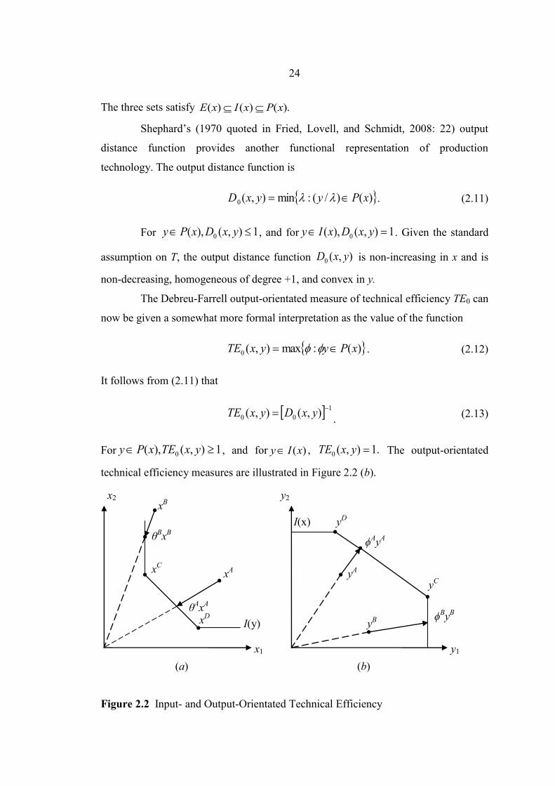
technical efficiency measures are illustrated in Figure 2.2 (b).

Figure 2.2 Input- and Output-Orientated Technical Efficiency

x1

I(y)

xB

xA x

C

θBx

B

θAx

A

y1

y2

I(x)

ϕAy

A

ϕBy

B

yD

yA

yB

(a) (b)

xD

yC

x2

25

In figure 2.2 (a), the input vectors xA and x

B are on the interior of L(y), and

both can be contracted radially and still remain capable of producing output vector y.

Input vectors xCand x

D cannot be contracted radially and still remain capable of

producing output vector y because they are located in the input isoquant I(y); hence,

),(),,(max1),(),( B

I

A

I

D

I

C

I xyTExyTExyTExyTE . Since the radially-scaled

input vector θBx

B contains slack in input x2, there may be some hesitancy in describing

input vector θBx

B as being technically efficient in the production of output vector y.

No such problem occurs with radially-scaled input vector θAx

A. Thus, ( , )A A

ITE y x

( , ) 1B B

ITE y x even through )(yEx AA but ).(yExBB

In Figure 2.2 (b), illustrated output-orientated technical efficiency, the output

vectors yC and y

D are technically efficient given input usage x, and output vectors y

A

and yB are not. Radially-scaled output vectors ϕ

A y

A and ϕ

B y

B are technically efficient,

even though slack in output y2 remains at ϕBy

B. Thus, ( , )A A

OTE y x

( , ) 1B B

OTE y x even though )(xEy AA but )(xEy BB .

A scale efficiency (SE) measurement can be used to indicate the amount by

which productivity can be increased by moving to the point of the technically-optimal

productive scale (TOPS). Figure 2.3 depicts a technically-inefficiency firm operating

at point D*, and describes how scale efficiency can be calculated using an input-

orientated technical efficiency. The productivity of firm D* improved by moving

from point D* to point E on the variable returns to scale (VRS) frontier (i.e. removing

technical inefficiency), and it could be further improved by moving from point E to

point B (i.e. removing scale inefficiency).

26

Figure 2.3 Scale Efficiency

The ratio of the slope of ray 0D* to the slope of ray 0E is equal to the ratio

GE/GD*, and that the ratio of the slope of ray 0E to the slope of ray 0F (which also

equals the slope of ray 0B) is equal to the ratio GF/GE. Thus, one can use distance

measures to calculate these productivity differences. That is, the technical efficiency

of firm D* relates to the distance function from the observed data point to the VRS

technology and is equal to the ratio

TEVRS = GE/GD*. (2.14)

Furthermore, the scale efficiency of firm D* relates to the distance function

from the technically efficient data point, E to the CRS (or cone) technology and is

equal to

SE = GF/GE. (2.15)

In the DEA literature, the SE measure is usually not obtained directly, but is

calculated indirectly by noting that if one calculates the distance from the observed

data point to the CRS technology,

TECRS = GF/GD*. (2.16)

It can then be used to calculate the SE score residually as

0 x

q

D*

B

CRS Frontier

VRS Frontier

E F G

xD xF xE

27

SE = TECRS/TEVRS = (GF/GD*)/(GE/GD*) = GF/GE. (2.17)

Furthermore, the DEA literature often reports the TE(CRS) measure since it

provides a measure of the overall or aggregate productivity improvement that is

possible if the firm is able to alter its scale of operation, given that a firm is usually

unable to alter its scale of operation in the short run. One could view the TE(VRS)

score as a reflection of what can be achieved in the short run and the TE(CRS) score

as something that relates more to the long run (Coelli, Rao, O’Donnell and Battese,

2005: 60).

The measurement of scale efficiency in the multi-inputs, multi-outputs case

is a generalization of the above concepts. For a particular firm using an input vector, x

to produce an output vector, y the concept of TOPS are related to the finding a point

of maximum productivity on the production frontier, subject to the constraint that the

inputs and outputs mixes cannot be altered, but the scales of this vector can. Visually,

this involves finding all points (δx, λy) on the surface of the production technology,

where δ and λ are non-negative scalar. These points produce a two-dimensional

function similar to that in Figure 2.3. One would then obtain TOPS point

corresponding to those particular inputs and outputs mix.

The Debreu-Farrell measures of technical efficiency are widely used. They

satisfy several properties (Russell 1988, 1990 quoted in Fried, Lovell and Schmidt,

2008: 25). Among these properties are the following:

1. ),(1 xyTE is homogeneous of degree one in inputs, and ),(0 yxTE is

homogeneous of degree one in outputs.

2. ),(1 xyTE is weakly monotonically decreasing in inputs, and ),(0 yxTE is

weakly monotonically decreasing in outputs.

3. ),(1 xyTE and ),(0 yxTE are invariant with respect to changes in units of

measurement.

A notable feature of the Debreu-Farrell measures of technical efficiency is

that they do not coincide with Koopmans’s definition of technical efficiency.

Koopmans’s definition is demanding, requiring the absence of coordinatewise

improvements (simultaneous membership in both efficient subsets), while the Debreu-

Farrell measures require only the absence of radial improvements (membership in

28

isoquants). Thus, although the Debreu-Farrell measures correctly identify all

Koopmans’ efficient producers as being technically efficient, they also define as being

technically efficient any other producers located on an isoquant outside the efficient

subset. Consequently, Debreu-Farrell technical efficiency is necessary, but not

sufficient for Koopmans technical efficiency. The possibilities are illustrated in

Figures 2.2, where θBx

B satisfy the Debreu-Farrell conditions but not the Koopmans

requirement because slacks remain at the optimal radial projection.

However, the practical significance of the problem depends on how many

observations lie outside the cone spanned by the relevant efficient subset. Hence, the

problem disappears in much econometric analysis, in which the parametric form of

the function used to estimate production technology (e.g. Cobb-Douglas, but not

flexible functional forms such as translog) imposes equality between isoquants and

efficient subsets, thereby eliminating slack by assuming it away. The problem

assumes greater significance in the mathematical programming approach, in which

the nonparametric form of the frontier used to estimate the boundary of the production

set imposes slack by a strong (or free) disposability assumption. The following

section will introduced the stochastic production frontier.

Two approaches of stochastic production frontiers models are historically

related to concept and application. For the first approach, suppose producers use

inputs Nx R to produce scalar output Ny R , with technology

iii vxfy exp);( , (2.18)

where β is a parameter vector characterizing the structure of production technology

and i = 1,…, I, indexes producers. The deterministic part of the production frontier

is );( ixf . Observed output yi is bounded above by the stochastic production

frontier, ii vxf exp);( , with the random disturbance term 0

iv included to capture

the effects of statistical noise on the observed output. The stochastic production

frontier reflects );( ixf in an environment influenced by external events, favorable

and unfavorable, beyond the control of producers or management ivexp .

29

The weak inequality in (2.18) can convert to equality through the

introduction of a second distribution term to create

iiii uvxfy exp);( , (2.19)

where the distribution term 0iu is included to capture the inefficiency effect on

observed output.

The Debreu-Farrell output-orientated measure of technical efficiency is the

ratio of maximum possible output to actual output.

1exp/exp);(),(0 iiiiii uyvxfyxTE , (2.20)

because 0iu . In order to estimate (2.20) one can estimate ),(0 ii yxTE in a number

of ways depending on the assumptions. It also requires a decomposition of residuals

into separate estimates of vi and ui.

One approach, first offered by Winsten (1957: 282-284) suggesting

Corrected Ordinary Least Squares (COLS), is to assume that ,,...,1,0 Iiui and that

vi~ ),0( 2

vN .In this case, (2.20) reduces to a standard regression model that can be

estimated by OLS. The estimated production function, which intersects the data, is

then shifted upward by adding the maximum positive residual to estimate intercept,

creating a production frontier that bounds the previous data. The residuals are

corrected in the opposite direction and becomemaxˆ 0i iv v , i = 1,…, I. The technical

efficiency of each producer is estimated from

ˆ( , ) exp 1,O i i iTE x y v (2.21)

and ( , ) 1 0O i iTE x y indicates the percentage by which output can be expanded, on

the assumption that .,...,1,0 Iiui

The producer having the largest positive OLS residual supports the COLS

production frontier. This makes COLS vulnerable to outliers, although ad hoc

sensitivity tests have been proposed. In addition, the structure of the COLS frontier is

identical to the structure of the OLS function, apart from the shifted intercept. This

30

structural similarity rules out the possibility that efficient producers are efficient

precisely because they exploit available economies and substitution possibilities that

average producers do not. Hence, the assumption that best practice is just like average

practice, but better, defies both common sense and much empirical evidence.

Finally, it is troubling that efficiency estimates for all producers are obtained

by suppressing the inefficiency error component ui and are determined exclusively by

the single producer having the most favorable noise max

iv . The term exp{ui} in (2.20)

is proxied by the term vexp in (2.21). Despite the fact that there have been

reservations expressed regarding the use of, COLS is widely used, presumably

because it is easy.

The second approach, suggested by Aigner and Chu (1968: 831-835), was to

make the opposite assumption, that .,...,1,0 Iivi In this case, (2.19) collapses to a

deterministic production frontier that can be estimated by linear or quadratic

programming techniques that minimize either i iu ori iu 2, subject to the

constraint that ,0/);(ln iii yxfu for all producers. The technical efficiency of

each firm is estimated from

ˆ( , ) exp 1,O i i iTE x y u (2.22)

and ( , ) 1 0O i iTE x y indicates the percentage by which output can be expanded, on

the alternative assumption that .,...,1,0 Iivi The iu values are estimates from the

slacks in the constraints Iiyxf ii ,...1,0ln);(ln of the program. Because no

distribution assumption is imposed on ,0iu statistical inference is precluded, and

consistency cannot be verified.

Following Schmidt (1976: 238-239), who showed that the linear

programming estimation of β is the maximum likelihood (ML) are appropriated, if the

iu values follow an exponential distribution. However, the quadratic programming

estimation of β is the maximum likelihood are appropriated, if the iu values follow a

half-normal distribution. Greene (1980 quoted in Fried, Lovell and Schmidt, 2008:

31

36) has demonstrated that an assumption that the iu values follow a gamma

distribution generates a well–behaved likelihood function that allows statistical

inference, although this model does not correspond to any known programming

problem. Despite the obvious statistical drawback resulting from its deterministic

formulation, the approach has gained in popularity since it is easy to append

monotonicity and curvature constraints to the program.

During the same period, independently proposed by Aigner et al. (1977

quoted in Fried, Lovell and Schmidt, 2008: 36) and Meeusen and Van den Broeck

(1977 quoted in Fried, Lovell, and Schmidt: 2008: 36), were attempted to remedy the

shortcoming of the previous approach with an approach known as Stochastic Frontier

Analysis (SFA). In this approach, it is assume that vi~ ),0( 2

vN and that 0iu

follows either a half-normal or an exponential distribution. The motive behind these

two distributional assumptions is to parsimoniously parameterize the notion that

relatively high efficiency is likely than relatively low efficiency. After all, the

structure of production is parameterized, and parameterizes the inefficiency

distribution too. Further, it is assumed that the vi and the ui values are independently

of each other and of xi. OLS can be used to obtain consistent estimates of the slope

parameters but not the intercept, because 0)()( iii uEuvE . However the OLS

residuals can be used to test for negative skewness, which is a test for the presence of

variation in technical inefficiency. If evidence of negative skewness is found, OLS

slope estimates can be used as starting values in a maximum likelihood routine.

It is possible to derive a likelihood function which can be maximized with

respect to all parameters ( ,, 2

v and 2

u ) to obtain consistent estimates of β. However,

even with this information, neither party is able to estimate ),(0 ii yxTE in (2.20)

because they are unable to disentangle the separate contributions of vi and ui to the

residual. Jondrow et al. (1982: 233-238) provided an initial solution by deriving the

conditional distribution of )(| iii uvu , which contains all the information (vi-ui)

contains about –ui. This enabled them to derive the expected value of this conditional

distribution, from which they proposed estimating the technical efficiency of each

producer from

32

1ˆ( , ) {exp{ [ | ( )}} 1,O i i i i iTE x y E u v u (2.23)

which is a function of the MLE parameter estimates. Later, Battese and Coelli (1988

quoted in Fried, Lovell, and Schmidt, 2008: 36-37) proposed estimating the technical

efficiency of each producer from

1ˆ( , ) { [exp{ }| ( )]} 1,O i i i i iTE x y E u v u (2.24)

which is a slightly different function of the same MLE parameter estimates and is

preferred because iu in (2.23) is only the first-order term in the power series

approximation to iuexp in (2.24).

In equations (2.23) and (2.24) efficiency estimation was unbiased.

Hypothesis tests have been frequently conducted on β and occasionally on 22 / vu to

test the statistical significance of efficiency variation. Horrace and Schmidt (1996:

261-265) and Bera and Sharma (1999: 196-201) were the first to develop confidence

intervals for efficiency estimates, but afterward did not gain popularity presumably

because the estimates of 22 / vu were relative small. In such circumstances, the

information contained in a ranking of estimated efficiency scores is limited,

frequently regarding the ability to distinguish good from bad producers.

Next, there are characteristics of the operating environment affect in

determining firm efficiency. The logic is that if efficiency is to be improved, one

needs to know what factors influence it, apart from the inputs and outputs. Two

approaches have been developed:

1. Let KRz be a vector of exogenous variables thought to be relevant to

the production activity. One approach that has been used within and outside the

frontier field is to replace );( ixf with ),;( ii zxf , z serving as a proxy for technical

change that shifts the production frontier but does not influence the efficiency of

production.

2. It was common practice to adopt a two-stage approach to the

incorporation of potential determinants of productive efficiency. In this approach,

efficiency was estimated during the first stage using either (2.23) or (2.24), and

estimated efficiencies were regressed against a vector of potential influences during

33

the second stage. Deprins and Simar (1989 quoted in Fried, Lovell and Schmidt,

2008: 39) were perhaps the first to question the statistical validity of this two-stage

approach. Later, Battese and Coelli (1995: 326-28) proposed a single-stage model of

general form

;exp);( iiiii zuvxfy , (2.25)

where 0; izu and z are vector of potential influence with parameter vector ,

and they showed how to estimate the model in SFA format. Later, Wang and Schmidt

(2002: 134-143) analyzed alternative specifications for );( ii zu in the single-stage

approach. They also provided theoretical arguments supposed by compelling Monte

Carlo evidence, explaining the biasness of the two-stage procedure. Later, with the

high capacity of computer computation, there was the advancement of the Bayesian

method that could be applied to efficiency analysis.

Since the early 1960s, Bayesian econometric had developed rapidly after the

publication of Bayes’ essay in 1763; since then, there has been an upswell of work in

Bayesian econometrics. Now, the Bayesian learning model is utilized in many works

in economic theory (Zellner, 1985: 253-254). Koop (2003:1-11) provides an overview

of Bayesian econometrics introducing the Bayes’ rule, which is basic to Bayesian

econometrics:

)(

)()|()|(

Ap

BpBApABp (2.26)

Let y be a vector or matrix of data and θ be a vector or matrix which contains

the parameters for a model which seeks to explain y,

)(

)()|()|(

yp

pypyp

. (2.27)

The econometric involves learning about the coefficients in the regression

(unknown) given data (known) and the conditional probability of the unknown given

the known. One can be interested in learning about θ and ignore the term p(y) since it

does not involve θ. Now, write:

34

)()|()|( pypyp . (2.28)

The term )|( yp is referred to as the posterior density for the data given the

parameters of the model, )|( yp as the likelihood function and )(p as prior density.

The prior )(p contains any non-data information available about θ. It summarizes

the knowing of θ prior to obtaining the data. As an example, suppose θ is a parameter

which reflects returns to scale in a production process. In many cases, it is reasonable

to assume that returns to scale are roughly constant. One can have prior information

about θ before looking at the data that would expect it to be approximated.

The likelihood function, )|( yp , is the density of the data conditional on the

parameters of the model. It is often referred to as the data generating process. For

instance, in the linear regression model, it is common to assume that the errors have a

normal distribution. This implies that )|( yp is a Normal density, which depends

upon the parameters (i.e. the regression coefficients and the error variance). The

posterior, )|( yp , is the density which is of fundamental interest. It summarizes all

that is known about θ after (i.e. posterior to) seeing the data. Equation (2.28) can be

thought of as an updating rule, where the data allow us to update our prior views

about θ. The result is a posterior which combines both data and non-data information.

That is, given the observed data, y, we may predict some future unobserved data y*.

Bayesian reasoning says that one should summarize uncertainty about what one does

not know (i.e. y*) through a conditional probability statement. That is, prediction

should be based on the predictive density, p(y*|y), and a marginal density can be

obtained from a joint density through integration:

dypyypyyp )|(),|*()|( (2.29)

Suppose, one use the mean of the posterior density as a point estimate, and

suppose θ is a vector with k elements, ),...,( 1 k . The posterior mean of any

element of θ is calculated (mostly by computer) as

dypyE ii )|()|( . (2.30)

35

In addition to a point estimate, it is usually desirable to present a measure of

uncertainty associated with the point estimate. The most common such measure is the

posterior standard deviation, which is the square root of the posterior variance

calculated as 22 )|()|()|var( yEyEy iii ,

which requires evaluation of the

integral in (2.30), as well as dypyE ii )|()|( 22

.

All of these posterior features which the Bayesian may wish to calculate have

the form:

dypgygE )|()(]|)([ , (2.31)

where )(g is the function. For instance, ig )( when calculating the posterior

mean of i and ( ) 1g ( 0)i when calculating the probability that i is positive,

where 1(A) is the indicator function which equals 1 if condition A holds and equals

zero otherwise. Even the predictive density in (2.31) falls in this framework if

set ,|*)( yypg . An implication of the law of large numbers is the Monte Carlo

integration.

Let s for s = 1, S be a random sample from yp | , and define

S

s

s

S gS

g1

1ˆ . (2.32)

Then Sg converges to ygE | as S goes to infinity. Equation (2.32) allows us to

approximate ygE | by averaging the function evaluated in the random sample.

This sampling from the posterior is referred to as posterior simulation and s is

referred to as a draw or replication. The simplest posterior simulator and use of this

theorem to approximate ygE | is referred to as the Monte Carlo integration. It

can be used to approximate ygE | , but only if S were infinite would the

approximation error go to zero. There are many ways of gauging the approximation

error associated with a particular value of S;

20 gs ,Ny|gEgS (2.30)

36

as S goes to infinity, where y|gvarg 2.

2.2.2 Previous Studies

The empirical study of efficiency difference involves determining the

relations of production function and measure distance to the frontier of these

individual observations. In analyzing production frontier models in education, the use

of the production function rather than the cost function may be more practical since

input prices generally are not available. Haushek (1986: 1142) acknowledges this

difficulty of efficiency measurement in the educational setting and states that

efficiency is ―a concept which has a very clear meaning in textbook analysis of the

theory of the firm but that becomes quite cloudy in the world of public schools.‖

Moreover, Engret (1996: 250) summarizes the complexity of the educational process

in terms of evaluating efficiency. First, the educational organization has multiple

objectives and multiple outputs and outcomes in satisfying stakeholders. Second,

many of the outputs of an educational organization cannot be unambiguously

quantified. Finally, we have limited knowledge of the true correspondence of inputs to

outputs. Numerous studies have dealt with the education production function for a

number of reasons; the true relationship, however, may never be clearly understood.

The study of Charnes, Cooper and Rhodes (1981: 668) may be one of the

first to utilize data from Program Follow Through (PFT), a large scale social

experiment in public school education, which was designed to test the advantage of

PFT relative to designated Non-Follow Through (NFT) counterparts in various parts

of the U.S. The DEA was therefore undertaken to distinguish between ―management

efficiency‖ and ―program efficiency.‖ The claimed superiority of PFT has failed to be

validated. The application of, however, suggests the additional possibility of new

approaches obtained from PFT-NFT combinations which may be superior to either of

them alone. The results of a DEA approach may be to guide further studies.

Bessent, Bessent, Kennington, and Reagan (1982: 1355) applied the DEA

to 167 elementary schools in the Houston independent school district. Of these

37

schools, 78 were found to be inefficient in utilizing their resources as compared to 89

efficient schools. The resources of this study were determined by budgets, teacher

assignments, and student assignments, while learning was determined by various

outputs scored according to standardized tests, such as the Iowa test of basic skills.

Smith and Mayston (1987: 181) employed a data envelopment analysis to show how

the data underlying performance indicators can be used to generate a single measure

of efficiency for an agency. The method systematically adjusts for differences in the

environment that different agencies face. It provides an interpretation for pursuing

efficiency in the public sector that the performance indicators has been published for

individual agencies, however, it remains unclear how these indicators should be

interpreted in isolation.

Sengupta and Sfeir (1988: 285-293) estimated the education production

function of selected public elementary school districts in California for 1976–1977

and 1977–1978; the study showed that these schools has increasing returns to scale.

Although the frontier was estimated, it specified the lower values of the overall scale

economy. This lends support to the hypothesis of an optimal school size model, where

schools operate in the region of increasing returns to scale subject to the limit of

availability of the student population. Ray (1991: 1620) combined a data

Envelopment Analysis (DEA) with regression modeling to estimate the relative

efficiency in the public school districts of Connecticut. The factors affecting

achievement were classified as school inputs and other socioeconomic factors. The

DEA was performed with the school inputs only. Efficiency measures obtained from

the DEA were subsequently related to the socioeconomic factors in a regression

model with a one-sided disturbance term. The findings suggested that while

productivity of school inputs varies considerably across districts, this can be ascribed

to a large extent to differences in the socioeconomic background of the communities

served. Variation in managerial efficiency was much less than what was only implied

by the DEA results.

Despite the interest in the impact of uncontrollable inputs on observed

educational efficiency, only one study has compared the results obtained from the two

alternative approaches. Using a sample of 27 poor, urban New Jersey school districts,

McCarty and Yaisawarng (1993: 277-284) explored both ways of incorporating

38

students’ socioeconomic status into a DEA model. The first model used the two-stage

approach, in which a Tobit analysis was employed to eliminate the effects of

socioeconomic status on a particular district’s efficiency scores. The second model

incorporated both controllable and uncontrollable inputs in the DEA computation of

efficiency scores. McCarty and Yaisawarng (1993: 285) found that the two models

produced ―similar results in the sense that the rankings of their efficiency scores are

positively and significantly correlated.‖

BonesrØnning and RattsØ (1994: 289) have applied this approach to the

measurement of the performance of the regulated school system in Norway analyzing

the relationship between resource use and student achievement in 34 Norwegian high

schools. The marginal school effect on student achievement was estimated, and the

output of the schools was described by the number of graduates and school effect.

Using this separation between quantity and quality, a reference frontier representing

best practice among the schools was established by data envelopment analysis, and

the technical efficiencies were measured. The schools exhibited very different student

achievements, but the variation did not relate to differences in resources use. The

school system was orientated towards the equalization of student results, but the

schools showed systematic differences in the handling of high and low achievers.

Ruggiero (1996: 553) showed that the consequences of not controlling for

these fixed factors were biased estimates of technical efficiency. The mathematical

programming approach to frontier estimation, was extended to allow for

environmental variables. This modified model was then contrasted with the existing

model that purportedly controlled for exogenous factors to measure public sector

efficiency with simulated data. The results of the analysis of the technical efficiency

of school districts provided evidence that the existing data envelopment analysis

model overestimated the level of technical inefficiency and that the modified model

developed in this paper has done a better job of controlling for exogenous factors.

Duncombe et al. (1997: 1) empirically tested bureaucratic models of supply

by drawing on the measurement literature. In anticipation of the results, it was found

that there existed empirical evidence supporting some of the implications of these

models. Kirjavainer and Loikkanen (1998: 377) argued that the lack of identifiable

statistical properties, the effect of school uncontrollable factor such as student’s

39

socioeconomic status will affects student achievement. They also suggested a two-

stage procedure which uses the DEA to calculate the efficiency scores using variables

that are controlled by the school’s administrators, while the second stage involves the

use of the maximum likelihood (ML) estimation of the Tobit regression model

measure based on variables that are not included in the DEA and are possibly outside

the administrator power of schools.

Phongsakornnoppadol (2005: 79) employed the DEA measure of technical

efficiency of Thai primary and lower secondary schools. The second-stage Tobit

regression model was used to determine the correlation of efficiency scores with

exogenous factors. The results suggest that most of the primary and secondary schools

are relatively inefficient. However, a larger school size tends to more efficient. Private

schools seem to be more efficient. In addition, the location of the school has

significantly correlates with school efficiency. It is suggested from the study that, not

only do school inputs but also exogenous factors significantly influence school

efficiency. Dechpolmat (2005: 107) measured the operational efficiency of various

types of municipalities in Thailand using the DEA analysis. The result indicated that a

large-type of municipality which is relatively bigger in size is more efficient than a

general-type of municipality. The analysis of the inefficiency of ―input usage‖

suggests that the small size municipality utilizes the central budget efficiently;

however, the medium size municipality utilizes inputs such as expenditures,

payments, and material efficient. It was also suggested from the study that there is a

correlation between expenditure and efficiency. The optimal inputs mix would

increase municipality production close to the frontier; however, the number of

efficient municipalities remains the same.

Rassouli-Currier (2007a: 53) employed a stochastic frontier regression (SFR)

estimating the inefficiency model simultaneously with the production or cost function.

In the DEA model, the first stage estimated the efficiency scores and the second stage

used a Tobit regression model to determine the causes of inefficiency. The literature

suggests that the empirical results of the SFR and DEA efficiency scores for the

majority of Oklahoma school districts were not identical, suggesting that the method

of estimation affects the efficiency scores. In general, the SFR generated a more

favourable score than that of the DEA. The results from the two estimation methods

40

in the inefficiency model were also different. However, both methods suggest that the

most important determinants of inefficiency are the socioeconomic factors associated

with each district. Rassouli-Currier (2007b: 131) analysed the efficiency of the

Oklahoma school districts using two different specifications measured by the DEA

method. In order to determine the possible sources of inefficiency, a second stage

Tobit regression was employed. Here, the specification of the inefficiency models

included: (i) environmental variables that school districts have no control over (e.g.

the percentage of students in special education and the poverty rate in the district),

and (ii) non-traditional inputs that school districts do have control over (e.g. teachers’

salaries) but were not included in the first stage DEA. The findings of the models

were compared and both suggested that the key factors affecting efficiency measures

among the Oklahoma school districts were primarily the students’ characteristics and

family environment.

There is some literature that employs Bayesian econometrics for measuring

efficiency. Ahmad and Bravo-Ureta (1996: 399), for example, examined the impact of

the fixed effects production frontier against stochastic production frontiers regarding

technical efficiency measures using an unbalanced panel consisting of 96 Vermont

dairy farmers for the 1971-1984 period in the analysis. The models examined

incorporated both time-variant and time-invariant technical efficiency. The finding

was that the major source of variation in efficiency levels across models stemmed

from the assumption made concerning the distribution of the one-sided term in the

stochastic frontiers. In general, the fixed effects technique was found to be superior to

the stochastic production frontier methodology. The overall conclusion of the study,

however, was that the efficiency analysis was fairly consistent throughout all of the

models considered.

Osiewalski and Steel (1998: 103) described the use of modern numerical

integration methods for making posterior inferences in composed error stochastic

frontier models for panel data or individual cross-sections. Two Monte Carlo methods

were used in practical applications and they argued that the Gibbs sampling methods

can greatly reduce the computational difficulties involved in analysing such models.

Later, Kim and Schmidt (2000: 91) compared the point estimates and confidence

intervals for technical efficiency levels. Classical procedures include ―multiple

41

comparisons with the best,‖ based on the fixed effects estimates, and a univariate

version, ―marginal comparisons with the best,‖ bootstrapping of the fixed effects

estimates, and maximum likelihood given a distributional assumption. Bayesian

procedures include a Bayesian version of the fixed effects model, and various

Bayesian models with informative priors for efficiency. They found that fixed effects

models generally perform poorly and that there is a large payoff distributional

assumption for efficiency. There is a great difference between Bayesian and classical

procedures in the sense that the classical maximum likelihood estimation based on a

distributional assumption for efficiencies yields results that are rather similar to a

Bayesian analysis with the corresponding prior.

Balcombe, Iain, and Jae (2006: 2221) estimated and examined the

technical efficiency of a cross-section of Australian dairy farms using various

methods; Bayesian, classical stochastic frontiers, and data envelopment analysis. The

results indicated technical inefficiency was present in the sample data. There was a

statistical difference between the point estimates of technical efficiency generated by

the various methodologies. However, the rank of farm level technical efficiency was

statistically invariant to the estimation technique employed. Finally, when confidence

intervals of technical efficiency were compared, a significant overlap was found for

many of the farms’ intervals for all frontier methods employed. The results indicate

that the choice of estimation methodology may matter, but that the explanatory power

of all frontier methods is significantly weaker when the interval estimate of technical

efficiency is examined. In sum, there is an array of techniques that can estimate

efficiency frontier, including DEA, SFA and Bayesian Stochastic Frontier Analysis

(BSFA). SFA and BSFA are ostensibly differentiated from each other by statistical

paradigms which not only lead to differences in interpretation, but also to the idea that

important theoretical properties can be enforced (O’Donnell and Coelli, 2005:520).

In this study, the frontier estimation was extended to allow for leakage and

weak institutional capacity variables. This modified model was then contrasted with

the existing model that used to measure public sector efficiency. Chapter 3 presents

the frame of reference that the study will use in the analysis.

CHAPTER 3

FRAME OF REFERENCE

I often say that when you can measure what you are speaking about, and

express it in numbers, you know something about it; but when you cannot

measure it, when you cannot express it in numbers, your knowledge is of a

meager and unsatisfactory kind. If you cannot measure it, you cannot

improve it (Kelvin, Lord, 2009).

Institutions are “the rules of the game in a society, or more formally, [the]

humanly devised constraints that shape human interaction” (North, 1990: 3). The

public sector has generally taken on responsibility for delivery of services to citizens

and uses public service bureaucracies as the instrument. For any individual service

transaction to be successful there needs to be a frontline provider that is capable, that

has access to adequate resources and inputs, and that is motivated to pursue

achievable goals. The general question is: What institutional conditions support the

emergence of capable, motivated frontline providers with clear objectives and

adequate resources? The answer: successful services for poor people emerge from

institutional relationships in which the actors are accountable to each other (World

Bank, 2003: 46). This chapter describes the frame of reference used in the study.

43

3.1 The Service Delivery Framework

The center is the relationship; there are five features of relationships among

service delivery actors which are presented as follows (World Bank, 2004: 48);

Delegating: explicit or implicit understanding that a service (or goods

embodying the service) will be supplied,

Financing: as the first step in creating a relationship of accountability,

providing the resources to enable the service to be provided or paying for it,

Performing: supplying the actual service,

Having information about performance: obtaining relevant information and

evaluating performance against expectations, formal or informal norms, and

Enforcing: being able to impose sanctions for inappropriate performance or

providing rewards when performance is appropriate.

Figure 3.1 Five Features of the Accountability Relationship

Source: Adapted from World Bank (2003: 47).

Figure 3.1 illustrates the relationships of accountability among actors in

terms of five features (delegating, financing, performing, informing, and enforcing),

Actors

(principals)

including

clients, citizens

policymakers

Accountable

actors (agents)

including

policymakers,

providers

Financing

Performing

Informing

Enforcing

Delegating

Accountability relationship

44

actors including clients and citizens and accountable actors including policymakers

and providers. According to these features, the accountability relationships can be

explained as taking a job; a person is given a set of tasks (delegating) and paid a

salary (financing), and the employee works (performs). The contribution of the

employee is assessed (informing). Based on that information, the employer acts to

reinforce good or discourage bad performance (enforcing). The accountability

relationship is formed as the service delivery framework, The next section describes

the important elements of the service delivery framework.

3.1.1 The Four Actors

The roles of the actors in the chain of service delivery consist of the

following: citizens/clients, politicians/policymakers, organizational providers, and

frontline professionals. Weakness in any relationship or in the capacity of the actors

can result in service failures. Figure 3.2 illustrates these relationships.

Figure 3.2 Service Delivery Framework

Source: World Bank, 2003: 49.

The State

Politicians Policymaker

s

Citizens/Clients Providers

Non-poor Poor

Short route

of accountability

Client power

Long route

of accountability

Service

Management

Voic

e

Com

pact

Frontline Organizations

Coalitions/inclusion

45

1. Citizens/clients; as citizens, they participate both as individuals and

through coalitions in the political process that defines collective objectives. They

strive to control and direct public action in accomplishing these objectives. As direct

clients of service providers, individuals and households hope to obtain quality public

service.

2. Politicians/policymakers; politicians control the state power and discharge

fundamental responsibilities. The other actors that exercise the power of the state are

policymakers. Politicians set general directions, but policymakers set the fundamental

rules of the game for service providers to operate.

3. Organizational providers; a provider organization can be a public line

organization such as ministry, department, and agency. It can be a ministry of

education that provides educational services. It can be large (public sector ministries

with tens of thousands of teachers) or small (a single, community-run primary

school). For frontline providers, all services require a provider that comes in direct

contact with clients, including teachers, doctors, nurses, and so on. The policymaker

sets and enforces the rules of the games of organization providers and the head of the

provider creates internal “policies” specific to the organization.

There are also three main relationships of power among the state,

citizens/clients, and providers. Each actor has a complex accountability relationship

between them. These relationships can be explained as follows.

1. Voice; the complex relationships of accountability between citizens and

politicians. Voice is about politics, but it covers the relationship of formal political

mechanisms and informal ones. Delegating and financing between citizens and states

involve decisions about pursuing collective objectives and mobilizing public

resources to meet these objectives. Citizens need information in order to understand

the actions of the state that can promote their welfare. At the same time, if politicians

do not pursue objectives effectively, citizens need some mechanisms whereby they

can make politicians and policymakers accountable to them.

2. Compact; the relationships between policymakers and service providers.

This does not mean legally enforceable as a contract. It is a broad agreement about a

long-term relationship. The policymakers provide resources and delegate powers to

the service providers and generate reports on organizational performance. The

46

policymakers specify the rewards and penalties depending on the actions and

outcomes of the providers.

3. Client power; the form of demand of services that citizens reveal to

providers. Citizens monitor the provider’s provision of services. Clients and

organizational providers interact through the individuals that provide services, such as

frontline professionals and workers.

There are mechanisms that actors use to influence the service delivery

procedures. These mechanisms can be explained as follows:

1. Management; this is a tool in every organization, providing frontline

workers with assignments and delineated areas of responsibility. In public agencies

this management function is complex comparison with the private sector because

providers are employees of “the government;” however, general management issues

of selecting, training, and motivating workers still apply.

2. Coalitions/inclusion; in societies where the average citizen is poor,

politicians faces strong incentives to address the general interest. However, in

clientelist political environments, even though the average citizen is poor, politicians

have strong incentives to shift public spending to cater to the special interests of core

supporters. When the average citizen is poor, catering to special interests at the cost of

the general interest is clientelism. Making services work for poor people is obviously

more difficult in a clientelist environment than in a pro-poor environment. When

populations are heterogeneous, it matters whose voices politicians/policymakers hear

and that they respond to citizens.

The strength of relationships and the mechanisms within the actors, as

explained in the foregoing section, underpin the success of the service delivery

framework. In the education context, this facilitating of government expenditure

translates into desire outcomes.

3.1.2 The Market

The “market” is an idealized set of relationships of accountability based on

choice, backed by purchasing power. The market has several strengths and

47

weaknesses in the provision of services. One strength is that customers will buy where

they perceive satisfaction, and organizations have incentives to respond to them.

Another strength is that organizations can manage their frontline provider as they

wish. However, the market has three weaknesses; it responds exclusively to customer

power so there are no pressures for equity in the allocation of services; it will not

satisfy collective objectives in general; and it can be effective in having customer

power discipline the providers, but only when the customer has the relevant

information about provider performance. However, in a competitive market, the

“customer’s loyalty” may be one of the contributing factors in the decision to

purchase goods and services.

A competitive market automatically creates the accountability of sellers to

buyers. The key information is customer satisfaction, and the key enforceability is the

customer’s choice of supplier. “Competitive markets have proved a remarkably robust

institutional arrangement for meeting individual interests,” but they are not enough for

services for three reasons (World Bank, 2003; 6).

1. The market responds only to those with purchasing power, doing nothing

to ensure universal access or equitable distribution, which societies often have as a

collective objective.

2. The sum of the individual interests may not produce the best outcomes

because markets may have failures of various kinds.

3. Other collective objectives may require public action. For instance, the

state and society have a strong concern about the role of schooling in the socialization

of youth and may not want parents to choose for themselves.

The public service is difficult to monitor, called the “monitoring problem,”

since locally-produced services such as basic education have some characteristics that

make it particularly difficult to structure the relationships of accountability.

Classroom teaching is transaction-intensive, and the transaction requires discretion,

presenting challenges for any relationship of accountability because it is difficult to

know whether the provider has performed well. It is difficult to monitor the millions

of daily interactions of teachers with students. As a result, rigid, script rules would not

provide enough latitude in the case of multi-principals and multi-tasks, in which

public servants serve many masters.

48

There are two types of accountability: long route and short route

accountability, however, in order to achieve satisfying outcomes, either relationship

has to be strong. The extension attempt to shorten long route accountably, the

so-called “sub-national government” model, is described in the next section.

3.1.3 The “Sub-national Government” Model

Gropello (2004: 3-4) has proposed the “sub-national government” framework

for analyzing decentralization reforms in the education sector in Latin America by

applying the accountability relationship framework. This model places an

intermediate political actor at the center of the decentralization process. There are big

differences in some countries in adopting the model. Argentina and Brazil, for

example, have transferred many more responsibilities to the sub-national level

(virtually all responsibilities for the administration of personnel and non-personnel

costs, extensive responsibilities in financing, and some responsibilities in planning the

educational process and setting-up curricula) compared with Chile and Mexico, which

have maintained fairly centralized personnel and financing policies. The driving force

in this type of model was to decentralize the main responsibility for the delivery

process. Central to the working of this model are two main accountability

relationships: the “compact” relationship between the center and the regional or local

political actor, and the “voice” relationship between the citizens and the regional or

local political actors.

According to this framework, the traditional long route accountability model

of service provision usually exhibits failures and limitations. The greater reliance will

be placed on more direct client influence or the short route accountability model.

Understanding the actors and the relationships of accountability for the success and

failure of centralized public service production created new institutional arrangement

for service provision, where regional or local political actors work more closely with

organization providers.

49

Figure 3.3 The “Sub-national Government” Model

Source: Adapted from Gropello (2004: 3).

Accountability “has been a dominant, if not the dominant, concern for the

designers of democratic political systems” (Peters, 1996: 112). Andrews (2005 quoted

in Shah, ed., 2005: 218-219) argued that the links between voice and another

dimension of the expanded version of accountability cause the government in

developing countries to free the expression of social voice in their governance

process. A developmental approach has emerged that concentrates on the

development of mechanisms and tools that facilitate voice expression at the local and

regional levels. In this concentration, “A wide range of mechanisms” is seen to “serve

as agents of accountability” (Blair, 2000: 27). Such mechanisms are designed to

provide regular channels, “windows” or “dedicated bodies,” through which citizens

can access governments (Schneider, 1999: 530). The extent of voice expression in

poor groups can influence urban government structures, which obviously influence

the nature of “pro-poor” policies and activities (Mitlin, 2000: 7).

The State

Politicians Policymaker

s

Citizens/Clients Providers

Non-poor Poor Frontline

Client power

Service Organizations

Management Coalitions/inclusion

Policymakers

Sub-national Govt. V

oic

e

Com

pact

Com

pact

50

There are two factors that influence accountability and that are useful in

identifying outcomes associated with the adoption of voice mechanisms. First, voice

influence relates to the degree to which voice, as expressed through a voice

mechanism, affects who governs, how they govern, what they consider, and what they

produce. Cases in which influence is high also appear to be the cases in which

positive accountability effects are observed. Cases in which influence is low also

appear to be the cases in which accountability effects are absent.

3.1.4 School-Based Management

School-based management (SBM) presents a conceptual framework for the

analysis of decentralization reforms, including the mechanisms through which SBM is

thought to improve outcomes (such as student achievement or parental participation).

Malen, Ogawa, and Kranz (1990: 290 quoted in Barrera-Osorio, Tazeen, Harry and

Lucrecia, 2009: 15) have stated that “school-based management can be viewed

conceptually as a formal alteration of governance structures, as a form of

decentralization that identifies the individual school as the primary unit of

improvement and relies on the redistribution of decision-making authority as the

primary means through which improvement might be stimulated and sustained.”

Thus, in SBM, responsibility for and decision-making authority over school

operations are transferred to principals, teachers, parents, students and other

community members. However, these school-level actors have to operate within a set

of policies determined by the central government.

In SBM framework, the accountability of school principals (service

providers) is upward to the ministry (politicians/policymakers) that holds them

responsible for providing services to the clients (parents/students) who, in turn, have

put the politicians/policymakers in power and thus have the voice to hold them

accountable for their performance. In most cases of SBM, the management

mechanism change under the reform process. The clients themselves become part of

the management; as a result, short route accountability becomes shorter, as the

representative of the clients (either parents or community members) have the

51

authority to make decisions and a voice in decisions that directly influence school

attendance. The SBM framework was introduced whereby the school administrator,

whether the head teacher alone or a committee of parents and teachers, acts as the

accountable entity. This power and management of the client creates the “non-market

direct link.”

Figure 3.4 School-Based Management and Four Accountability Relationships

Source: Adapted from Barrera-Osorio et al. (2009: 31).

One can expect greater parent involvement when implementing SBM, in

which the schools are more responsive to the interests of children. Parents will then

more greatly value schooling and their students’ academic achievement. SBM reforms

do not necessarily give more power to general public officials, because the power

devolved by the reform is susceptible to capture by elites. Bardhan and Mookherjee

(2000: 135-139, 2006: 101-127) and Bardhan (2002: 185-205) suggest that local

The state

Politician

s

Policymaker

s

Citizens/Clients Providers

Non-poor Poor Frontline

Long route of accountability

Service

Organizations

Management Coalitions/inclusion

Voic

e

Com

pact

School committee

Clients Providers

Short route of accountability

Cli

ent

pow

er

Managem

ent

Clien

t pow

er

Managem

ent

52

democracy and political accountability often are weak in most of the developing

countries and can lead to elites capturing governance at various levels. To transfer

power to schools is to transfer it from somewhere else, and the entity that is losing

some of its power often is in a position to reverse its implementation if the reform

contravenes its original intent. Teachers themselves may be regarded as the ultimate

authority in a community; people that are given the responsibility for managing the

school may not have the capacity to do so. Finally, there are often challenges and

resistance during the implementing of SBM reforms.

3.2 Student Achievement Production Function

The student achievement production function can measure the influence of

family background, peers, school inputs, and innate abilities regarding student

achievement during the entire period that students attend school. The production

function at the level of an individual student can be written as follows:

* * *( ) ( ) ( ) *, , , ,t t t t t t t t

i i i i i iA FB PR IP IN A , (3.1)

where t

iA is a vector of variables measuring student i’s achievement at time t,

*( )t t

iFB is the vector of family background influences over the period t* to t, *( )t t

iPR is

the vector of influences of peers over the t* to t, iIN is the vector of innate abilities of

the i-th student, and *t

iA is the vector of the outcomes of the i-th student period. This

function evaluates the educational achievements of the student, not only in terms of

controllable inputs but also taking into account the influence of a student’s innate

abilities, former achievements, family background, and peers.

The model is convenient because it reduces data requirements. In the

empirical study of this model, the data may consist of information on individuals or it

may be aggregated at the school level; the units of observation are schools, and the

performance indicators measure the achievement of students in each school. The

53

following section presents the methods derived from the model described in equation

(3.1).

3.2.1 Data Envelopment Analysis (DEA)

Data envelopment analysis is a non-parametric method, where theoretically-

based hypotheses can be tested with classical tests. Hence, variables were constructed

which would be operational counterparts of some of the elements in (3.1) typically

used in the literature.

Mathematically, assuming that schools minimize the use of inputs given the

fix level of outputs by solving a linear optimization problem, the efficiency score of

the school can be calculated. Following Coelli et al. (2005: 180), the output-orientated

measure of technical efficiency is the solution to the constant returns to scale linear

programming problem, and can be expressed as:

,max , (3.2)

st 0,iy Y

0,ix X

0,.

Banker et al. (1984: 1085) have proposed a variable returns to scale linear

programming problem as follow:

,max , (3.3)

st 0,iy Y

0,ix X

1 1I

0,

where is a scalar, iy and ix are column vector of outputs, and column vectors of

inputs for the ith school, respectively. is a 1N vector of constants. The variable Y

is an M N output matrix, while X is a K N matrix in which 1 , and 1

is the proportional increase in outputs that can be achieved by the i-th firm, with input

quantities held constant. The 1I is a 1I vector of ones. This approach forms a convex

54

hull of intersecting planes that envelope the data points more tightly than the CRS

conical hull and thus provide technical efficiency scores that are greater than or equal

to those obtained using the CRS model. 1/ defines a TE score, which varies

between zero and one, and the output-orientated TE score reported by DEAP 2.1.

3.2.2 Stochastic Frontier Analysis (SFA)

The idea behind of the stochastic frontier analysis is to add an error term with

two components to the production frontier—one allows for random error and another

allows for technical inefficiency.

The stochastic production frontier model for cross-sectional data is

(x ; ) exp( )i i i iy f v TE , (3.4)

where iy is the output of producer i, 1,..., ,i I xi is the vector of K inputs used by the

producer i, is a vector of 1K technology parameters to be estimated, and

(x ; )i iy f is the deterministic production frontier. Further exp( )iv embodies the

random shocks on each producer, being that (x ; ) exp( )i if v is the stochastic

production frontier. Finally, TEi is the output-oriented technical efficiency of producer

i, defined as

,(x ; ) exp( )

ii

i i

yTE

f v

(3.5)

which is the ratio of observed outputs and the maximum feasible output conditions on

exp( )iv . Producer i attains the maximum feasible output if and only if TEi=1;

otherwise, 0 1iTE provides a measure of the shortfall of observed outputs from

the maximum feasible in an environment characterized byexp( )iv .

In order to estimate the stochastic production frontier model in (3.5), let

defined as exp( ),i iTE u

which 0iu to ensure that 1iTE and

specifying ( )f which is assumed to take a translog form because of its flexibility. The

55

translog production function can be estimated by maximum likelihood upon making

an assumption about the distributions of vi and ui. The original specification put

forward in the literature was the normal, half-normal model, which assumed that (i)

2~ (0, ),i vv iidN (ii) 2~ (0, )i uu iidN (i.e. as a truncation below 0 of a normal

distribution with mean 0 and variance 2

u ) and (iii) iv and iu independent of each

other and of the regressors. The normal, half-normal specification has been extended

to assume a more general distribution of iu . This study will use the normal-truncated

normal model, where the assumption (ii) above is replaced by

( )ii 2~ ( , )i uu iidN (i.e. as the truncation below 0 of a normal distribution with

mean and variance 2

u ). The advantage of this generalization is to allow more

observations to be farther from zero from the inefficiency term distribution.

The log-likelihood function to be maximized is based on the density

function ( )if for a sample of I producers and, prior to maximization, a re-

parameterization of the type 2 2 2

u v and 2 2 2/ ( )u u v is typically

introduced. The parameter measures the relative importance of 2

v and 2

u . If

0 either 2

v or 2 0 :u the two-sided error component would dominate

and the production frontier could be estimated by ordinary least square (OLS). If

1 either 2

u or 2 0v , the technical inefficiency component would

dominate and one would have a deterministic production frontier without noise. The

parameters 2( , ) are estimated together with the technology parameter in , and the

maximum likelihood estimators are consistent with I (number of producers). In the

context of SFA, testing the significance of assumes particular importance, since if

the null hypothesis 0 were accepted, no stochastic frontier methodology would be

necessary and all technology parameters could be consistently estimated by OLS.

Following Battese and Coelli (1992: 163), the log-likelihood function can be

maximized, based on the density function ( )if for a sample of I producers, and the

density functions can be expressed as:

56

2

2

1 ( )( ) exp ,

22 uu

u

u zg u

z

0u (3.6)

2

2

1( ) exp ,

42 v

vg v

v

v , (3.7)

where ( ) denotes the distribution function for the standard normal random variable;

the joint density function of u and v u is:

2 2

2 2 2

1 ( ) ( )exp

2( , )

2

v u v

u vu

u z

h uz

, (3.8)

where

2 2

2 2

u v

u v

z

and

2 22

2 2

u v

u v

. (3.9)

Integrating the joint density function ( , )h u over u yields the marginal density

function of :

2 222

20 2

0

1 1 ( )exp exp2 2( ) ( , )

22

v u

u v

u

z udu

f h u duz

(3.10)

Simplification of (3.10) yields:

2

2 2

12 2 2

1 ( )exp

2 (( )

2 ( )ˆ

v u

uv u

z

hz

. (3.11)

Using equations (3.8) and (3.11) the following condition density function of u given

can be expressed:

57

2

2

1 ( )exp

2( | ) .

2

u

f u

(3.12)

By adding subscription i and t, the conditional expectation of exp( )itu given it is

obtained from equation (3.12):

ˆ 1

( | ) exp .2

it

it

u

it it it

it

TE E e

(3.13)

The SFA makes it possible to estimate the degree of efficiency in the

utilization of inputs by producers. In order to gain further insight one may want to

carry the analysis relate to the producer performance with “exogenous” variables,

which are not at the discretion of the producer but nevertheless influence the outcome

of the production process (referred to as producer heterogeneity). Such variables

could for instance characterize the environment where productions take place. They

are not supposed to influence the shape or location of the production frontier, but

determine how far away the producer is from it, which refers to inefficiency

determinants. Several approaches have been suggested in the literature to incorporate

appropriately inefficiency effects into the SFA.

Follow Battese and Coelli (1993: 22); assumes that itu is a truncation below 0

of a normal distribution with mean 0 ,it m m itmz and variance 2 ,u where

mz are producers and time-specific variables that determine inefficiency. If 'm s are

equal to zero, the specification reduces to the Normal, Truncated-Normal model

above, with 0 , and can likewise be estimated by maximum likelihood. Following

Battese and Coelli (1995) consider a generalized frontier production function for

education as:

exp( )it it it ity x v u , (3.14)

58

where ity denotes the output of the i-th school in the t-th time period, itx represent a

(1 )k vector of inputs and other explanatory variables for the i-th school in the t-th

time, is a ( 1)k vector of unknown parameters to be estimated, 'itv s are assumed

to be 2~ (0, )iid N random variables associated with the technical efficiency of

production. Technical inefficiency itu in equation (3.14) is further defined as:

it it itu z c , (3.15)

where itz is a (1 )M vector of explanatory variables associated with technical

inefficiency effects, is an ( 1)M vector of unknown parameters, and itc is non-

negative observed random variable obtain by truncation of the 2~ (0, )it cc N such

that .it itc z This is an alternative specification of itu being a non-negative

truncation of the 2( , ).itN z

3.2.3 Bayesian Stochastic Frontier Analysis (BSFA)

Let ity and it denote the t-th observations on the dependent variable and

error, respectively, for the i-th individual. In some of the regressions, it is important to

distinguish between the intercept and slope coefficients. Hence, define iX to be a

kT matrix containing the T observations on each of the k explanatory variables

(including the intercept) for the i-th individual. iX~

will be the 1 kT matrix equal

to iX with the intercept removed. Hence, iTi XX~

. Stack the observations for all

N individuals together, obtaining the TN-vectors:

Nyyy ...1 and N ...1 .

Similarly, stacking observations on all explanatory variables together yields the

KTN matrix,

NXXX ...1 .

59

Assuming that each firm has a particular efficiency level over time, defined

the production model where output of firm i at time t, Yit, using a vector of inputs,

*

itX , (i = 1,…,N, t=1,…,T). Firms have access to a common best-practice technology

for turning inputs into outputs. This technology depends upon a vector of unknown

parameters, , and is given by:

;XfY *

itit . (3.17)

This so-called production frontier measures the maximum amount of output

that can be obtained from a given level of inputs. In practice, actual output of a firm

may fall below the maximum possible. The deviation of actual from maximum

feasible output is a measure of inefficiency, and can be stated as:

i

*

itit ;XfY , (3.18)

where 10 i is a measure of firm-specific efficiency and 1i indicates that firm

i is fully efficient. A value of, say, 800.i means that firm i was producing 80%

of the output it could have if it were operating according to best-practice technology.

Following Koop (2003: 168), allow for a random error in the model, it , to

capture specification error, resulting in:

it

*

itit ;XfY . (3.19)

The inclusion of measurement error makes the stochastic; hence the name stochastic

frontier model. If the production frontier ( )f is log-linear (e.g. Cobb-Douglas or

translog), take logs and write as:

iititit zXy , (3.20)

where k,..., 1 , itit Ylny , itit ln , ii lnz and itX is of the

counterpart *

itX with the inputs transformed to logarithms. iz

is referred to as

inefficiency and, since 10 i , it is a non-negative random variable. itX is assumed

to contain an intercept and isi its coefficient. Note that this model is of the form of

60

an individual effects model. However, in the stochastic frontier model, economic

theory gives us some guidance in selecting a hierarchical prior. If the production

function is not log-linear (e.g. the constant elasticity of scale production functions),

stacking all variables into matrices, equation (3.20) can be written as:

Tiiii zXy (3.21)

where T is our notation for a T-vector of ones.

The form of the likelihood function depends upon assumptions made about

the error. Assume that iz and j are independent of one another for all i and j. The

resulting likelihood function is:

TiiiiTiii

N

iT

T

zXyzXyhh

zhyp

)(2

exp

2

,,|1 2

2

(3.22)

where Nzzz ,...,1 . Treating z as a vector of unknown parameters which enter the

likelihood function, likelihood function was defined as:

dzzpzhyphyp |,,|,,| ,

where |p z is a distributional assumption for the inefficiencies, which depends

upon a vector of unknown parameters, θ. But such a procedure is mathematically

equivalent to the Bayesian procedure of using ( | )p z as a hierarchical prior.

For the coefficients in the production frontier, and error precision, the

independent normal-gamma prior was applied as:

~ ( , )N V (3.23)

and

2~ ( , )h G s v . (3.24)

For the inefficiency effect, a hierarchical prior was used, since 0iz , the

Normal hierarchical prior was not suitable. Hence the derivation of Bayesian

inference in stochastic frontier models using exponential distribution was

61

appropriated; which is a gamma distribution with two degrees of freedom. Thus, we

assume that iz and jz are a priori independent for i j with

~ ( ,2)i Zz G . (3.25)

The hierarchical nature of the prior means, treat the mean of the inefficiency

distribution as a parameter which requires its own prior. Since 0iz , it follows

that 0z . In the same way, working with error precision (h) instead of error

variance 2 allows us to stay in the familiar class of error distributions; it is easier

to work with 1

z instead of z . A prior form can be written as,

1 1~ ( , )z z zG v . (3.26)

The hyper-parameters 1

z

and zv can often be elicited through consideration

of the efficiency distribution. That is, the prior information about the location of the

efficiency distribution was already known. Let * denote the prior median of this

distribution. If firms in the study are expected quite efficient, * could be set to a high

value (e.g. 0.95). On the contrary, if many firms are expected inefficient, * could be

set to a lower value.

In the individual effect models, posterior inference can be carried out by

setting up a Gibb sampler. Since the Gibbs sampler requires only full conditional

posterior distributions with the relevant conditional distributions, except for the ones

relating to z and z , were the same as those of the individual effects model with

hierarchical prior. For the parameters in the production frontier, obtain,

| , , , ~ ( , )zy h z N V , (3.27)

where

1

1

1

N

i i

i

V v h X X

and

1

1

N

i i i T

i

V V h X y z

.

62

For the error precision:

2| , , , ~ ( , )zh y z G s v (3.28)

v TN v

and

2

2 1

( ) ( )N

i i T i i i T i

i

y z X y z X vs

sv

.

The posterior conditionals for the inefficiencies are independent of one another (i.e.

iz and jz are independent for i j ) and are each Normal, truncated to be positive

with post density function, given by

1 1( | , , , ) ( | ( ) ,( ) )1( 0)i i z N i i i z ip z y h f z X y Th Th z , (3.29)

where 1

T

itti

yy

T

and

iX is a 1 k matrix containing the average value of each

explanatory variable for individual i. Remember that 1 ( 0)iz is the indicator

function which equals 1if ( 0)iz and is otherwise 0.

The posterior condition for 1

z is given by

1| , , , ( , )z z zy h z G v (3.30)

2 zv N v

and

1

2z

z N

i z

i

vN

z

.

A Gibbs sampler which involves sequentially drawing from (3.28) through

(3.30) can be used to carry out Bayesian inference in the stochastic frontier model.

In this chapter, the frame of reference was introduced; therefore, producing

three methods of interest for estimation. The DEA is a non-parametric method,

showing how inputs directly affect student academic achievement; however, SFA and

63

BSFA are parametric methods that incorporate exogenous variables in the framework.

The next chapter will present the research methodology of the study.

CHAPTER 4

RESEARCH METHODOLOGY

“...in order for a writer to produce something which is original and correct, it

is not absolutely necessary that his predecessors have been wrong.”

William J. Baumol (1964: 1081)

In Thailand, little is known about how public expenditure flows through the

budget system across bureaucratic structure. This study attempts to generate new

knowledge of how resources flow through the administrative level, what the

magnitudes of the public resources are, and how those resources are combined with

other inputs at the facility level to produce desirable educational outcomes.

4.1 Public Expenditure Tracking Survey and Quantitative Service

Delivery Survey

This study is a case study, focusing on the small-sized schools of northeast

Thailand. The methodology of expenditure tracking survey is fairly straightforward

and consists of first, a thorough charting of the budget flows through various

government levels. Next, a series of quantitative assessments, using survey

instruments, of budgets flows in and out these of the government is carried out.

65

The goal is to explicitly track funds that are allocated to education down to

the level of the school, and schools are surveyed concerning the amount of public

financial support they receive.

The amounts can then be matched and compared to allocated and distributed

amounts. Since a large share of public funding in the education sector is through the

payment of teacher salaries and transfer through personal bank accounts, there is little

chance of leaks. Consequently, non-wage funds are included in the study.

There are two types of service provider surveys that complement each other,

the Public Expenditure Tracking Survey (PETS) and Quantitative Service Delivery

Survey (QSDS), which have been developed to address questions of the efficiency

and equity of public expenditure and service delivery.

A PETS tracks the flow of resources through these strata to determine how

much of the originally-allocated resources reach each administrative level. It is

therefore useful as a device for locating and quantifying political and bureaucratic

capture, leakage of public funds, and problems in the development of human and in-

kind resources, such as staff and textbooks. It can also be used to evaluate

impediments to the reverse flow of information (weak accountability relationship) in

order to account for actual expenditures. Consequently, PETS could be used as a

diagnostic tool, an analytics tool, and as a tool for policy effectiveness evaluation.

1. Regarding PETS as a diagnostic tool, a diagnostic survey seeks to

ascertain concrete facts and to identify basic problems without necessarily exploring

why problems are occurring or the solution. The problem that PETS studies have

diagnosed are leakage of public funds, usually non-wage subsidies. Studying this

problem involves the collection of a sufficient amount of data within well-designed

samples. A simple calculation of expenditure leakage can be expressed as

Leakage =Funds recieved by facility

Funds intend for the facility. (4.1)

2. Regarding PETS as an analytical tool, it is important to understand the

causes of the institutional problems. A starting place for analysis may be the

observation that the capture of funds varies across schools and perhaps across districts

and regions. The task that falls to analysis is to determine the factors that are

66

correlated with the variable of interest, and to formulate and test the hypotheses

discerning the causal relationships. If the causes are discovered, the appropriate policy

intervention is often implied.

3. Finally, regarding PETS as an impact evaluation tool, following the

previous purpose, a third reason to conduct a PETS is to examine the impact of a

policy intervention that has already taken place. The likely occasion to use a PETS for

impact evaluation is after an earlier PETS, so that the results of a subsequent PETS

can be compared.

A QSDS has the primary aim of examining weak institutional efficacy,

particularly the efficiency of public spending, dissipation of resources, and incentives

and various dimensions of service delivery in provider organizations, especially at the

front line. It collects data on inputs, outputs, quality, pricing, oversight, and so forth.

The facility or front line service provider is typically the main unit of observation.

The Ministry of Education is responsible for promoting and overseeing all

levels and types of education. Local administration has been involved in education

administration, especially at the basic level.

There are ministries that undertake the management of education in

specialized fields, or for specific purposes. Hence, conducted by the state, the local

administration organization (LAO) and educational administration and management

in Thailand are thus administered as follows (Figure 4.1). The Education Service Area

(ESA) was established in order to decentralize the administration of education, each

ESA being responsible for approximately 200 schools. At the time of the survey, there

were 185 ESAs across the country.

67

Figure 4.1 Educational Administrations and Management Structure

Source: Adapted from OEC (2008: 32).

The resources flowing in social sectors are complex. The various resources

required for service delivery (financial resources, human resources, and in-kind

transfers) originate from several sources (central government ministries, decentralized

administrative levels, bilateral and multilateral donors) and take various routes in the

organizational system. In addition, these flows are generally governed by different

allocation rules, administrative processes, recording and accounting procedures, etc.

An essential initial stage in any tracking surveys is thus to identify and analyze the

Ministry

of Education

Ministry

of Interior

Other

Ministries

providing

specialized

education

Formulation of

policies, plans,

standards; support of

resources;

monitoring and

evaluation

Independent Agencies/

Government-Supervised

Agencies

Higher Education

Institutions

Educational

Service Areas

Local

Administration

Organization

Public units

providing

education

Supervision,

support, and

promotion in

response to

policies and

standards

Implementation/

administration,

and management

Institutions

providing

basic and

early

Childhood

education

Agencies,

organizations/

individuals

responsible for

educational

provision

Educational Institutions

Agencies

and

institutions

providing

specialized

education

Direct line of authority

Support, Promotion and Coordination

68

nature and characteristics of these various administrative structures and flows in order

to grasp their role and contribution to service providers’ resources.

According to the PETS and QSDS survey, resources flow through two

administrative levels, that is the OBEC and ESA. The resource flows in the

administrative system do not follow a simple top-down approach. At each level, funds

may be received directly from the central government. The LAO can also support the

approved school project. The ESA also uses public expenditure, for example, when

schools purchase materials from merchandisers; they will send the evidence to the

ESA, and the electronic settlement process of this billing is carried out and money is

paid directly to the seller (Figure 4.2).

Figure 4.2 Flow of Fund in Education Sector

Source: PETS-QSDS 2007 survey

Ministry of Education/

Office of Basic Education Commission (OBEC)

(Central Government)

Education Service Area

(District Administration)

School

(Service Providers)

Donors

Households

(Clients/Citizen)

Subsidy flow

Staff remuneration

School fees

Stores

69

At the time of the study, there were two types of public expenditure

entitlements from the OBEC that have been included in this study: (i) rule-based

expenditure—all funds were allocated directly to schools; (ii) discretionary funds,

allocated from the OBEC to ESA, then allocated to the schools upon committee

approach. In addition, some of the incurred fees were paid by households that

financed the school for a particular project.

A school subsidy was carried out twice a year on a semester basis: fiscal year

2006 covering semester 2/2005 and 1/2006, and fiscal year 2007 covering semester

2/2006 and 2/2007. Hence, capitation grant leakages can be calculated on an academic

basis, where academic year 2006 covers semester 1/2006 and 2/2006. Typically,

public expenditures reach the school at about 80% (front-load allocation) before the

semester begins. There were claims that the “free education” policy had been

resurrected; however, there has been tremendous confusion over whether parents were

required to pay any fees at all. There is evidence, however, that a significant

proportion of schools have not tried to raise resources from parents. Previous studies

have reported that PETS and QSDS reveal a leakage in the financial data available at

schools. This was not for lack of effort on the part of the PETS and QSDS survey but

primarily reflects the record keeping at the school level. For a large number of

schools, the available financial information was incomplete.

4.2 Sample Selection and Data Collection

The primary data used in this study come from new, cross-sectional surveys

that cover school, household, and student aspects of grade 9 in the northeastern part of

Thailand, in Nakornratchasema and Amnatcharoen.

Nakhonratchsema is located approximately 260 kilometers northeast of

Bangkok, and the city itself serves as the gateway to the lower northeastern region.

Geographically, Nakhonratchasema is the largest northeastern province; as an

administrative center, Nakhonratchasema's role today remains unchanged, as it is

currently the main transportation, industrial, and economic hub of the region. In 2006,

70

the gross provincial product was 134,007 million baht (NESDB 2009:1), where 17.1%

was in the agricultural sector and 82.8% was in non-agricultural sector. Regarding

education, about 79.8% of the population between 3-17 years of age enrolled in

school, the proportion of the population aged 3-5 years that entered kindergarten or

preprimary school was 66.5%, 80.9% of children aged 6-11 years entered primary

school, 92% aged 12-14 years entered lower secondary school, and 41.29% of

students 15-17 years of age entered upper secondary school.

Amnatcharoen is located about 568 kilometers from Bangkok; the geography

is generally defined as tropical savannah. It has a high temperature all year round,

especially in the hot season, which starts in February to April, the rainy season starts

from May to mid-October, and the winter season starts from November to January.

There are 7 districts, 56 sub-districts, and 607 villages in the province. The

administrations consist of 1 provincial administration, 1 municipality, and 8 municipal

districts. The proportion of people living in the municipality is 16.6%, and the rest

live outside the municipality. According to the National Economic of Social and

Development Board’s compilation (NESDB, 2009:1), the GPP in 1988 price was

12,490 million baht and GPP per capita was 29,474 baht, ranking number 75 in the

country and number 18 in the northeast region. There are 300 schools, 3,303 teachers,

and about 67,735 students in Amnatcharoen. The post lower secondary education

consists of 6 institutions and 6,539 students.

The sampling design is generally referred to as a two-stage stratified cluster

sample. The sampling units at each stage are defined as follows. The first-stage

sampling units consisted of individual, small-size schools that have an average

number of students, ranging from 200 to 300 students. These schools are so-called

“expand-opportunity schools” and provide a compulsory education where students

will leave the school after they finish their lower secondary education. The second

stage included a visitation to the sample school, and careful interviewing techniques

and data quality determined the success of the study. The visitations began in

November 2008 for Amnatcharoen, followed by Nakhonratchasema province, and the

survey was completed in March 2009.

By using the systemic random sampling from the school roster, 109 schools

in 8 education service areas (ESA) across 2 provinces were visited. Table 4.1

71

illustrates the number of sample schools; however, there was a discrepancy in the

number of samples, in particular, ESA 2. An explanation is that most of the sample

schools in ESA 2 are located on the main road, which is convenient to visit, and ESA

2 was the starting point of the ESA survey so these schools in this district had plenty

of time to fill out the questionnaires. Hence, a proportion of usable questionnaires

were drawn from ESA 2.

Table 4.1 Samples Included in the Study

Province ESA Population Sample

Nakhonratchasema ESA 1 37 8

ESA 2 46 21

ESA 3 58 4

ESA 4 54 7

ESA 5 70 7

ESA 6 53 7

ESA 7 79 8

Amnatcharoen ESA 1 55 47

Total

109

During the survey period, there were several intermittent closures. The

questionnaire package was sent to the sample schools before visitation. Many of the

schools in the original sample could not be covered for a variety of reasons. In these

cases, replacement schools (randomly selected from the same district) were used as

substitutes. A special effort was made to ensure coverage of remote schools. In

particular, some schools were visited several times due to logistical difficulties.

Furthermore, there were some incomplete questionnaires that had to be excluded from

the analysis; for the econometric analysis, the total sampled schools of both provinces

in this analysis was reduced to 70 schools.

Chapter 2 discusses the weak institutional capacity that can occur with front

line service providers. In a weak accountability relationship environment, respondents

may lack incentives to provide correct feedback, so that multi-angular data collection

was used in the study. Consequently, the instruments were developed to ask various

72

responders the same set of questions. There were several purposes to survey

instrument; first, school-level instruments, which cover topics such as school

finances, school characteristics, teacher characteristics, student characteristics,

personnel management, and how the classroom teacher instruction. Instruments were

also designed to collect data on the roles and responsibilities in educational

administration, and these instruments were administered as a part of the school-level

instruments to head teachers and other teachers. In addition, the instruments were

administered to the ESA director. The instruments were designed to “track” fund flow

in the education system. The goal of the instruments was to track public fund

disbursement at the central level and at the school; the topics, including payroll,

education subsidy, and capitation grant. The idea was to capture the magnitude of

money leaving the central level and entering the district level, and delays in subsidy

disbursements.

The survey used a series of instruments for collecting data, including a

school survey, a grade 9 teacher survey, a board of management (BOM) survey, a

parent survey, and an ESA survey. Finalizing the instruments involved both thorough

reviews of questions, as well as field testing, to ensure that the questions were

understandable for the respondents. The results of an initial field testing of a few

schools were evaluated before the survey took place. However, not all instruments

could be completed for all schools; key respondents for particular instruments were

sometimes not available for several reasons, including questionnaire loss and

unwillingness to answer some questions. Table 3.2 presents the sample coverage by

type of instrument.

73

Table 4.2 Number of School Coverage by Type of Questionnaires

ESA Total number Number of Number of Number of Number of Number of

of school) Head Teacher ESA BOM Gr.9 Teacher Parents

Nakhonratchasema

ESA1 8 8 1 4 4 4

ESA2 21 21 1 21 20 18

ESA3 4 4 1 3 4 3

ESA4 7 7 1 5 5 4

ESA5 7 7 1 4 4 3

ESA6 7 7 1 4 4 4

ESA7 8 8 1 6 6 5

Amnatcharoen

ESA1 47 47 1 45 42 40

Some qualitative questions were intended to complement the quantitative

data. The motivation for the complement survey was that the contrasts in the

experience of schools across these diverse setting could offer additional insights into

the complex structure determining service delivery. Data collection involved

investigating two major focus areas of the study: problems and priorities of

institutional arrangements, including the community. The complete set of

questionnaires used in this study was attached in the appendix.

4.3 Variables for Production Function Estimation

The following describes the key variables of interest that were needed to

estimate the equation (3.1). Table 4.3 presents a detailed description of all variables

available for estimation.

The proxy of inputs (X) included the data that could be controlled by the

school administrator, which are the capitation grants (PG). PG is the main financial

resources of the school; the grant for pre-primary, primary, and lower secondary

74

education was 1,700, 1,900, and 3,500 baht annually. The average capitation grant of

these 3 levels was 2,367 baht annually. The other capitation grant was the

fundamentally-needed fund (FF), which targets poor students. This has been defined

as students whose family earns an income under 40,000 baht per year. These students

were eligible for this aid upon committee approved. This additional capitation for

primary education and lower secondary education was 460 and 2,500 baht annually,

respectively.

The other input variables were the student attendance rate (SA), where the

number of students present in class was compared with the classroom roster. The

teacher was assumed to be the key inputs that affected student achievement, other

things constant, and the teacher’s experience (EXP) could lead to student

achievement. The student-teacher ratio was used as a proxy for class size (CS); the

variable was defined as number of students per classroom.

The proxy of outputs (Y) was comprised of the average school test scores;

mathematics (MATH), science (SCIENCE), the Thai language (THAI), social studies

(SOCIAL), and the English language (ENGLISH).

Several other variables, socioeconomic or institutional factors (Z), were

needed to estimate the production function (Table 4.3). It is often believed that

females have more innate reading ability, while males are more skillful in

mathematics. Age may be an indicator of ability if older children have more time to

develop their innate skill. First-born children are also believed to have higher innate

ability, at least partly due to lower maternal nutrient depletion (King, 2003: 1732S).

Also, parental education is used as an indicator of a child’s ability if innate parental

ability affects the parents’ own level of education and is inherited by the child.

Moreover, there is evidence that the mother’s age when the child is born has a

biological effect on the child’s innate ability. Specifically, early childbearing has a

negative biological impact on children’s innate ability, although social factors also

play a role (Pevalin, 2003: 11-14). To capture the impact of children’s innate ability,

proportion of female student in the school (FEMALE), and parental education

(PARENTEDU), were included in the analysis. In addition, capturing the influence of

peers on learning achievement, the heterogeneity of students which proxy by the

standard deviation of the test scores (HETERO) was included in the equation.

75

Table 4.3 Description of Variables Used

Variables Descriptions Mean SD Unit

Inputs (X)

PG Avg. capitation grants received 472,982 242,695 baht

FF Avg. fundamentally-needed received 139,519 91,642 baht

SA Student attendance rate 90.41 16.59 percent

EXP Teacher experience 19.13 4.99 number of teaching year

CS Student/teacher ratio 16.86 4.67 no. of student/class

Outputs (Y)

THAI Avg. Thai language test scores 41.66 4.40 percent

MATH Avg. Mathematics test scores 28.49 4.49 percent

SCIENCE Avg. Science test scores 37.34 6.83 percent

ENGLISH Avg. English Language test scores 28.81 5.22 percent

SOCIAL Avg. Social Studies test scores 39.07 5.37 percent

Socioeconomic/Institutional (Z)

PROVINCE Province dummy 0.50 0.00 1=Nakhonratchasema

POLITICIAN Politicians’ involvement dummy 0.34 0.49 1=Involve

VACANT Teacher vacancy rate 6.30 8.02 percent

ABSENT Teacher absence rate 6.68 3.52 percent

SCHOOLSIZE School size 6.49 5.08 classroom/100 students

LKPERCAP Mismatch capitation grants 32,875 69,733 Baht

LKFUNDNEED Mismatch fundamentally-needed funds 10,638.50 28,025.85 Baht

FEMALE Share of female students 47.11 3.13 percent

HETERO Heterogeneity 3.47 0.45 standard deviation

BITUMEN Nearest bitumen road 1.85 3.93 kilometer

PARTICIPATION Parent meeting with school 0.62 0.20 proportion (0 to 1)

INCOME Household average income 4,638 1,528 baht/month

PARENT Living with parent 0.50 0.51 1= live with parent

PARENTEDU Parent’s education 9.43 2.76 year of schooling

INSPECTION Number of Inspections 7.20 5.15 times

Additional Variables

PAYDELAY Compensation delay 0.3 0.47 1=delay

DISDELAY Disbursement delay 5.8 7.3 day

ACCESS Access to facilities 8.41 3.90 kilometer

BOM Board of management meeting 4.3 2.74 times/annual

CLCONDITION Classroom condition 0.11 0.11 proportion (0 to 1)

INFRASTRUCT School infrastructure 0.54 0.22 proportion (0 to 1)

TCRESOURCE Teaching resources 0.34 0.12 proportion (0 to 1)

CLFACILITY Classroom facilities 0.78 0.21 proportion (0 to 1)

WATER School water and sanitation 0.60 0.15 proportion (0 to 1)

SECURITY School security 0.76 0.13 proportion (0 to 1)

76

The explanatory variables outside the power of the school administrator were

the following: leakage of capitation grants (LKPERCAP) and leakage of

fundamentally-needed funds (LKFUNDNEED), already defined in equation (4.1). The

school size (SCHOOLSIZE) variable was constructed by dividing total students by

total actual teachers in the school. In order to capture the effect of school location on

educational outcomes, the distance of the nearest bitumen road (BITUMEN) was

included in the study. The proxy of variables stemmed from weak institutional

capacity in the organizations; for example, the teacher absent rate (ABSENT), which

are teachers on the roster but were absent during the day of the survey was also

included in the study. In addition, the teacher vacancy rate (VACANT) could not have

been caused by weak institutional efficiencies; however, it was believed that this

factor affected student achievement, and consequently, sometimes the teachers

practiced the multi-grade teaching method.

There were also variables of interest that were associated with educational

outcomes; student’s socioeconomic status which proxy by household income

(INCOME), and the family environment which proxy by dummy variable (PARENT).

The other variables concerned the politician’s involvement (POLITICIAN) and

reflected the voice of citizens/clients. If politicians helped the school, the dummy

variable was set to 1 and 0 otherwise, and in order to distinguish the provincial effect

(PROVINCE), the Nakhonratchasema dummy variable was set to 1 and

Amnatcharoen was set to 0. In the SBM framework, parental participation

(PARTICIPATION) could shorten long route accountability; hence, the equation

included the number of parent meetings with the school. Finally, the proxy of

compact variable is number of school inspections (INSPECTION) from higher

authority.

In order to understand the associations among the variables of interest,

additional variables, combined with some of the forgoing variables, were included in

the correlation study. Compensation delay (PAYDELAY) was the dummy variable that

proxy of the delay in receiving the money, such as allowance, bonus, and academic

standing. Dummy value was set to 1 if there exists the compensation delay and 0

otherwise. Disbursement delay (DISDELAY) was defined as number of days after the

school’s budget got approved compared with school was able to use the budget.

77

Access to facilities (ACCESS) was the average distance of schools to important

places, such as secondary schools, health centers, stationary stores, post offices,

banks, bus terminals, public phones, etc. The number of meeting of school’s board

(BOM) was included in the study. The typical compositions of BOM are; head

teacher, parent, alumni, and other stakeholders.

The following variables were constructed as proportions (0 to 1). For

example, if the school supposed to has 100 textbooks, but data from the survey

reported that the school only has 30 textbooks, hence the proportion was set to 0.3.

These variables including classroom facilities (CLFACILITY), which was the average

of the proportion of the items in the classroom, such as: blackboard, teacher’s desk,

storage that can be locked, and electricity. School infrastructure (INFRASTRUCT)

was constructed by average proportions of the items in the school, such as:

administrative blocks, vehicle, land for agriculture and land for expansion, sport

areas, sport equipment, sciences laboratory, vocational laboratory, and a home

economics laboratory. The condition of the classroom (CLCONDITION) was the

proportion of classrooms that had been repaired, rebuilt, and the roof leaking when it

rained. Teaching resources (TCRESOURCE) were constructed by the proportion of

the usability of the library, textbooks, teacher’s room, teaching aids, students’ desks,

and teachers’ funds for producing teaching aids.

Finally, the study tested the effect on school environment, such as: water and

sanitation, and school’s security. The water and sanitation variable (WATER) was

constructed using the proportion of water tanks, reservoir, underground water,

adequate water on the day of the visit, all year availability, sufficient numbers of

toilets for the boys, and sufficient numbers of toilets for the girls. The proxy of

security variable (SECURITY) was number of times that school was not invaded by

intruders.

78

4.4 Limitations of the Study

Various methods have to be used when designing and implementing tracking

surveys. Each has consequences on the survey’s capacity to achieve its monitoring,

analysis, or evaluation purposes. The limitations of the study that are associated with

some of these issues include sample selection, length of data tracking, survey timing

and data sources, etc.

1. Any tracking survey requires determination on the specific flows from

which financial and quantitative information will be collected and at which

administrative levels. In each of the various branches or resource flows of the

allocation procedure, there are possibilities of leakage at various levels in the service

provision supply chain. Similarly, salary expenditures could leak through job capture.

However, not all flows are amenable to tracking. Non-existent records or accounts,

data inconsistencies, and other types of problems will make certain flows untraceable

or the data too noisy to be informative. Furthermore, the complexity and challenges of

tracking whole categories of expenditures have led PETS to restrict the tracking

exercise to focus on a subset of the entire service provider environment.

The entire spectrum of expenditures does not lend itself to tracking, either

because of poor quality data, recording procedures, disaggregated line items, a large

number of programs or sources of flows, or even survey budget constraints; one or a

few specific programs can be selected that lend themselves to tracking. Once the

items are identified, tracked was on the items sending and receiving end of at least

two levels, including service provider, in order to estimate leakage. All financial

flows during a certain time period had to be tracked.

2. With respect to service providers, the development of a representative

sample requires information on the population under study. Still most tracking

surveys have used this information to constitute an initial sample frame of the facility

population which was then, generally, verified and updated. Once the sample frame is

determined, sample stratification is often introduced, given the sample frame and

different types of facilities. As emphasized by Reinikka and Smith (2004: 55-56), at

least four issues have to be taken into account in the choice of a sample size. First, the

79

sample should be sufficiently large and diverse to represent the various types of

service providers. Second, some sub-categories may require more extensive sampling.

Third, the adequate sample size is a trade-off between minimizing sampling and non-

sampling errors. Non-sampling errors, which increase with sample size, are generally

more a concern than sampling errors in tracking surveys, as data are often in a highly

disaggregated form and hence difficult to collect. In addition, budget constraints must

also be taken into account in determining sample size. Furthermore, sampling design

becomes complicated when PETS and QSDS are jointly conducted. Indeed, in order

to adequately measure leakage in a PETS, it is better to sample a relatively large

number of local governments (districts); however, with a strict budget constraint, the

number of service providers sampled in each district was reduced. However, a QSDS

could be preferable to interviewing a greater number of facilities in a smaller number

of districts in order to assess differences in behaviour and performance among types

of facilities within districts.

3. It should be noted that short collection periods are generally associated

with problems of seasonality, which could bias the data. If data are collected on a

monthly basis, for instance, there is of course a need to aggregate the data on an

annual basis, while in the education sector there are few problems of seasonality. In

general, it is better to collect annual data if they exist instead of monthly data, except

if the issue of seasonality of services is specifically targeted as a management or

performance issue. One important element to consider is of course the fiscal year

period in use in the country. If the target is to obtain data on flows of funds over a

one-year period, these clearly have to correspond to the fiscal or academic year. The

tracking should in general always be done on at least the last completed fiscal year or

academic year. Ideally, the survey should be carried out two or three months after the

end of the fiscal year in order for accounting books to be closed. In any case, the

tracking should always be done on the preceding fiscal year, never on the current one.

This study collected data on fiscal year 2006-2007, which also covered academic year

2006; further, the length of quantitative data tracking was about 8 months. However,

there were several intermittent breaks from school closures during the survey and

obtaining past data needed required special effort on the part of the respondents.

80

4. Another issue which has implications for survey results and performance

relates to the source of the quantitative data collected. There has been some variance

among surveys in terms of data sources because in certain facilities, quantitative data

were based on recalls from the respondents instead of being based on accounts or

records. In order to minimize measurement errors, it is recommended that records be

used as much as possible. It should be noted that a missing record where information

could be very difficult to exactly gather, some information will be approximated by

the respondents.

In this chapter, the research methodology was introduced; the study employs

PETS and QSDS as research instruments. The variables used in the study included

inputs, outputs, and institutional factors that could affect the educational production

function. Chapter 5 will provide the details of the model estimation results.

CHAPTER 5

ESTIMATION RESULTS

A major challenge in any reform effort is the difficulty of operationalizing

the strategy. Several factors such as political will available resources,

committed reformers, collective action and coalition building among

stakeholders play significant roles in the success of such efforts (Kpendeh,

2009 quoted in Heidenheimer and Johnston, 2009: 430).

This following describes the estimation results, the calculation from the

survey data, and the econometric estimates of the production function. Specifically,

information on the leakage of public resources, which can be calculated using data

from the PETS, will be presented. The QSDS will provide the data regarding weak

institutional capacity. The results of the correlations studied, and the econometric

estimation of the variables, are summarized in this chapter.

5.1 Leakage and Weak Institutional Capacity

A schematic diagram of the flow of funds in the Thai education system at the

time of the survey is presented in Figure 5.1. At one end were three main financiers of

education: the government, the donors and non-governmental organizations, and

parents. At the other end are the “final recipients” of the funds: schools, teachers, and

non-teaching staff. The two ends were connected by different types of flow

mechanism.

82

Figure 5.1 The Flow of Funds in the Compulsory Educational Sector

Source: PETS-QSDS 2007 survey

The government subsidizes education through several channels. First, teacher

wages do not pass through school management. They are directly deposited into

teachers’ bank accounts. Payments to any non-teaching staff hired at schools (e.g. a

security guard, cleaner, or secretary) are the responsibility of the Board of

Management (BOM), and are typically financed by government subsidies. These

subsidies could be either in-kind or in-cash form. In-kind subsidies are school

materials, and in-cash subsidies are capitation grants and fundamentally-needed

funds. Second, the education subsidies were paid on a semester basis for supporting

operations. In practice, the Office of Basic Education Commission (OBEC) passed on

the subsidy amount to the Educational Service Area (ESA), which had the option of

Office of the Basic

Education Commission

(OBEC)

Educational

Service Area (ESA)

Donor,

NGOs

Parents

School

Non-teaching

staff

Teacher bank account

School

bank

account

Subsidy

School/Projects fees

Donations

Salary

In kind

Salary

Su

bsi

dy

Donations

Contractors or

Merchandisers

83

bulk buying school materials and distributing them to schools. The school would thus

receive in-kind subsidies supplied through contractors or merchandisers. The

Educational Service Area (ESA) itself could also take subsidies either in in-cash or in-

kind form. These grants may be absorbed in the ESA budget, which is further

supplemented with their own internal resources. Non-government financing (other

than parental contributions) can take the form of grants and donations from donors,

religious entities, non-government organization (NGO), private institutions, and

fundraising agencies. At the time of the survey, the parent-contributed subsidies were

school fees, depending upon the Board of Management (BOM) policy. The estimation

of leakage and weak institutional capacity relied on survey-based information;

however, it was typically incomplete or non-existent.

5.1.1 Leakage Estimation

Two types of in-cash subsidy entitlements from the OBEC have been

included in this study: (i) rule-based expenditure-capitation grants that are allocated

directly to schools; (ii) discretionary funds-fundamentally-needed that are allocated

from the OBEC to the ESA, and are then allocated to the schools upon committee

approved

The PETS-QSDS survey revealed leakage in the financial data available at

schools. Overall, the schools in Amnatcharoen leaked more than the schools in

Nakhonratchasema (Table 5.1).

For fiscal year (FY) 2006, the leakage of capitation grant was about 3.1%,

and leakage of fundamentally-needed funds was 7.3%. The figure looks similar for

FY 2007, where the leakage of capitation grants of schools in both provinces was

about 3.9%, and the schools in Amnatcharoen and Nakhonratchasema exhibited

leakages of fundamentally-needed funds at 7.2%, respectively.

84

Table 5.1 Leakages of In-cash Subsidies, FY 2006-2007

All (n=70) Nakhonratchasema (n=35) Amnatcharoen (n=35)

Mean (%) Mean (%) Mean (%)

Leakage of capitation grants …semester2/2005 2.7 3.0 2.5

…semester2/2006 3.5 3.8 3.2

Average FY 2006 3.1 3.4 2.8

Leakage of fundamental-needed funds …semester2/2005 6.3 1.5 11.0

…semester1/2006 8.3 5.6 11.0

Average FY 2006 7.3 3.5 11.0

Leakage of capitation grants …semester2/2006 3.9 4.0 3.7

…semester1/2007 3.9 3.3 4.3

Average FY 2007 3.9 3.7 4.0

Leakage of fundamental-needed funds …semester2/2006 6.9 2.1 11.7

…semester1/2007 7.5 4.3 10.6

Average FY 2007 7.2 3.2 11.2

Source: PETS-QSDS 2007 survey

Note: Leakage = Funds recieved by school

Funds intend for the school

The subsidies were disbursed before the semester began; fiscal year* 2006

covered semester 2/2005 and 1/2006, and fiscal year 2007 covered semester 2/2006

and 1/2007. In this study, the leakage of public expenditure was computed in terms of

academic year† (AY)-academic year 2006 was composed of semester 1/2006 and

2/2006. The leakage of capitation grants of schools in AY 2006 in both provinces was

about 3.7%, and a fundamentally-needed fund of schools in both provinces was about

8.0% (Table 5.2).

* Fiscal year is an accounting year, i.e. when the books for the year are opened and closed. It can

correspond to the calendar year or be, say, from October 1 to September 30. † Academic year is the period of days per year that students are attending classes. Normally, the first

semester is from May to September, and the second semester is from November to March.

85

The average amount of leakage of all types of capitation grants of sampled

schools in Nakornratchasema and Amnatcharoen was 28,100 baht and 24,800 baht,

respectively. Overall, the average amount of leakage of all schools in AY 2006 was

5.8% or about 52,900 baht.

Table 5.2 Average Leakages of In-cash Subsidies, %, and Amount, AY 2006

All Nakhonratchasema Amnatcharoen

(n=70) (n=35) (n=35)

Mean Amount Mean Amount Mean Amount

(%) (baht) (%) (baht) (%) (baht)

Leakage of capitation grants

…semester1/2006 3.5 16,800 3.8 10,100 3.2 6,700

…semester2/2006 3.9 18,500 4.0 10,700 3.7 7,800

Average 3.7 35,300 3.9 20,800 3.5 14,500

Leakage of fundamentally-needed

funds

…semester1/2006 8.4 10,300 5.6 5,300 11.1 5,000

…semester2/2006 6.9 7,300 2.1 2,000 11.7 5,300

Average 8.0 17,600 3.9 7,300 11.4 10,300

Average AY 2006 5.8 52,900 3.9 28,100 7.7 24,800

Source: PETS-QSDS 2007 survey

5.1.2 Absence Rate

Teachers can be absent for many reasons, for example because of illness, for

training, official duties besides teaching, as well as shirking; but from the perspective

of student learning achievement, the effects are the same. A teacher’s absence may

force the schools to find a substitute teacher to look after the children, or to send them

home. The PETS-QSDS assessed the extent of teacher absence regardless of the

causes, by taking a roster of all teachers that worked at the school and noting who was

not at school on the day of the visitation. The survey also reported the shortage of

teacher position longer than one semester for academic year 2006 and 2007. Table 5.3

86

summarizes the absence rate among all teachers from the roster, the vacancy rate, and

the shortage of teachers over one semester.

Table 5.3 Absence Rate, Vacant Teacher Position in The School and Shortage

of Teacher Over One Semester (%), AY 2006

All (n=87) Nakhonratchasema (n=44) Amnatcharoen (n=43)

Mean (%) SE Mean (%) SE Mean (%) SE

Absence rate 6 1 5 1 7 1

Vacant teacher position in the school

…academic year 2006* 17 3 9 1 23 5

…academic year 2007* 6 1 4 1 9 2

Average 12 2 7 1 16 4

Shortage of teacher over one semester

…academic year 2006* 49 7 55 10 43 9

…academic year 2007* 49 6 55 8 40 9

Average 49 7 55 9 42 9

Source: PETS-QSDS 2007 survey

Note: Average is based on items marked with*, SE is standard error.

The vacant teacher position in the school in AY2006 was 17%, with the

vacant teacher position at the schools in Amnatcharoen compared with

Nakhonratchasema being higher (23% compare to 9 %). Absence rate in AY 2007 in

Amnatcharoen and Nakhonratchasema was about 9%, and 4%, respectively. The

overall absence rate is 6%. It compares relatively well to similar surveys from other

countries; it was neither the lowest nor the highest rate observed. For example, in

Ecuador and Peru, 11% and 14% of teachers were absent on the day of the visit, and

in India and Uganda the absence rates were 25% and 27%, respectively (Section

2.1.1, page 15).

The survey indicates that the schools faced related problems of teacher

shortage. Regarding the difference in actual numbers of teachers and the number of

teachers supposed to be at work, the higher the different percentage the greater the

shortage. The measure is based on a direct response from the head teachers to the

87

question regarding whether the school experienced a shortage of teachers for more

than one semester. A 49% teacher shortage was reported. Schools from

Nakhonratchasema and Amnatcharoen were estimated at 55%, and 40%, respectively.

It is evidenced that remote areas need not have a higher shortage of teachers. The

overall average of teacher shortage was 49%, and this reflected a significant shortage

of teachers, which may affect student achievement.

5.1.3 Subsidy and Compensation Delays

School fee subsidies have continued to be politically popular, and this is in

part explained by the possible volatility in the amount of subsidy, especially for

school infrastructure, across the years. This high volatility in the absolute amounts of

the school subsidy has led to considerable uncertainty amongst different stakeholders

as to what subsidy to expect in any given year, in turn impacting negatively on the

planning process. The subsidies delays were examined using the information

regarding the budget disbursement data on the subsidies, and used direct information

on the disbursement time of the schools. The average delay was about 7 official days,

with the schools in Amnatcharoen and Nakhonratchasema reporting disbursement

delays of 8 days and 6 days, respectively (Table 5.4). There was a lot of variation

around the average; across schools, for example, some school reported disbursement

delays of 30 days, but some schools reported only 1 day. “Delays” were a source of

leakage; this goes hand-in-hand with uncertainty about the timing of subsidy receipts.

In the extreme case, cash-strapped schools have been forced down the path of some

school activity delays for a period of time. The potential source of disbursement

delays may due to administrative inefficiencies at the school, and more importantly at

the district and the national level. For example, districts were required to send in

acquittals and enrolment returns for the academic year so as to qualify for the subsidy.

88

Table 5.4 Subsidy and Compensation Delays

All (n=87) Nakornratchasema (n=44) Amnatcharoen (n=43)

Mean SE Mean SE Mean SE

Delays in being able to use subsidies (days)

...semester2/2005 6.89 1.17 5.39 1.15 8.36 1.86

...semester1/2006 6.70 1.14 5.59 1.18 8.36 1.86

...semester2/2006 6.70 1.14 5.59 1.21 7.51 1.77

...semester1/2007 6.89 1.17 5.59 1.21 7.84 1.81

Percent of teachers reporting

compensation delays

…academic year 2006 25 8 13 10 38 10

Average delay days 120 0.00 120 0.00 120 0.00

(for those experiencing delay)

Source: PETS-QSDS 2007 survey

Note: SE is standard error.

The teachers in an expanded-opportunity school get an average salary of

about 23,000 baht. There was a non-significant delay in the receipt of salary

payments. However, about 25% of teachers reported a compensation delay in things

other than salary, i.e. allowances they were eligible for such as bonus, and academic

standing. The average delay (for those experiencing delays) was about 120 days.

Proportions of teachers of schools in Amnatcharoen and Nakhonratchasema, 38% and

13%, respectively, reported delays.. These conditions are unlikely to generate a high

level of teacher motivation.

5.1.4 Correlation Study of Teacher Absence and Leakage

The hypothesis for the multivariate analysis was that teachers and school

characteristics do not affect the teacher’s absent rate. The dependent variable was

binary response, where 1 means that the teacher was present on the day of the survey,

and 0 otherwise.

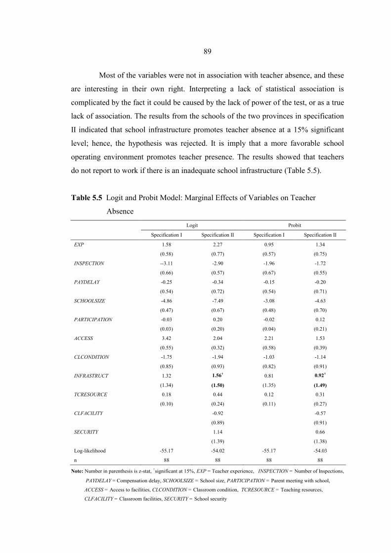
89

Most of the variables were not in association with teacher absence, and these

are interesting in their own right. Interpreting a lack of statistical association is

complicated by the fact it could be caused by the lack of power of the test, or as a true

lack of association. The results from the schools of the two provinces in specification

II indicated that school infrastructure promotes teacher absence at a 15% significant

level; hence, the hypothesis was rejected. It is imply that a more favorable school

operating environment promotes teacher presence. The results showed that teachers

do not report to work if there is an inadequate school infrastructure (Table 5.5).

Table 5.5 Logit and Probit Model: Marginal Effects of Variables on Teacher

Absence

Logit Probit

Specification I Specification II Specification I Specification II

EXP 1.58 2.27 0.95 1.34

(0.58) (0.77) (0.57) (0.75)

INSPECTION --3.11 -2.90 -1.96 -1.72

(0.66) (0.57) (0.67) (0.55)

PAYDELAY -0.25 -0.34 -0.15 -0.20

(0.54) (0.72) (0.54) (0.71)

SCHOOLSIZE -4.86 -7.49 -3.08 -4.63

(0.47) (0.67) (0.48) (0.70)

PARTICIPATION -0.03 0.20 -0.02 0.12

(0.03) (0.20) (0.04) (0.21)

ACCESS 3.42 2.04 2.21 1.53

(0.55) (0.32) (0.58) (0.39)

CLCONDITION -1.75 -1.94 -1.03 -1.14

(0.85) (0.93) (0.82) (0.91)

INFRASTRUCT 1.32 1.56† 0.81 0.92†

(1.34) (1.50) (1.35) (1.49)

TCRESOURCE 0.18 0.44 0.12 0.31

(0.10) (0.24) (0.11) (0.27)

CLFACILITY -0.92 -0.57

(0.89) (0.91)

SECURITY 1.14 0.66

(1.39) (1.38)

Log-likelihood -55.17 -54.02 -55.17 -54.03

n 88 88 88 88 Note: Number in parenthesis is z-stat, †significant at 15%, EXP = Teacher experience, INSPECTION = Number of Inspections,

PAYDELAY = Compensation delay, SCHOOLSIZE = School size, PARTICIPATION = Parent meeting with school,

ACCESS = Access to facilities, CLCONDITION = Classroom condition, TCRESOURCE = Teaching resources,

CLFACILITY = Classroom facilities, SECURITY = School security

90

Next, regression analysis was employed to explore the correlation of leakage

(capitation grant and fundamentally–needed funds) for AY 2006. Table 5.7 shows that

the OLS can be used for estimating the equation. The hypothesis of the model was

that there are no variables that correlate with leakage. The dependent variable of the

analysis was the leakage rate in the natural logarithms scale. Voice was proxied by

POLITICIAN, compact was proxied by INSPECTION, client power was proxied by

BOM, and management was proxied by ABSENT. Regarding other factors,

DISDELAY, PAYDELAY, ACCESS, VACANT, EXP, and PARTICIPATION (client

power) were included in the model. ACCESS was dropped in specification II, and

ACCESS and EXP in specification III. Only 70 schools providing data were included

in the model.

In all specifications, the hypothesis was rejected; there was a significant

difference between the provinces. Schools in Amnatcharoen seemed to have higher

leakage. Teacher absent rate promotes leakage and the coefficient was almost the

same. This implies that the higher teacher absence rate, the higher the leakage of per-

capitation grants. Specification I exhibits another significant contributing factor,

which was teacher experience. The school that has the more experienced teachers

tends to have a reduced leakage effect.

The results look different for fundamentally-needed funds. Payment delays

that are statistically significant correlate with leakage. However, specification II

implies that the province dummy was not significant in the model, and only payment

delay statistically and significantly explained the leakage. For specification III, the

factor that significantly explained the leakage of fundamentally-needed fund was

similar to specification I (Table 5.6).

91

Table 5.6 OLS Estimates of the Correlation of ln Leakage of Capitation Grants and

ln Leakage of Fundamentally-needed Funds, AY 2006

Capitation grants Fundamentally-needed fund

Specification I Specification II Specification III Specification I Specification II Specification III

PROVINCE -0.39** -0.50*** -0.50*** -0.28* -0.24 -0.25*

(2.54) (3.46) (3.53) (1.72) (1.60) (1.67)

POLITICIAN 0.19 0.04 0.04 -0.08 -0.09 -0.09

(0.16) (0.31) (0.33) (0.67) (0.74) (0.71)

DISDELAY -0.16 -0.16 -0.17 0.13 0.13 0.12

(1.32) (1.33) (1.37) (0.99) (1.00) (0.95)

PARTICIPATION 0.12 0.15 0.15 -0.02 -0.04 -0.04

(0.97) (1.19) (1.18) (0.19) (0.28) (0.33)

VACANT 0.05 0.03 0.03 0.11 0.12 0.13

(0.41) (0.21) (0.25) (0.86) (0.95) (1.03)

ABSENT 0.27* 0.25* 0.25* 0.05 0.06 0.06

(1.96) (1.78) (1.78) (0.36) (0.43) (0.41)

INSPECTION 0.10 0.14 0.14 -0.12 -0.13 -0.13

(0.85) (1.18) (1.22) (0.95) (1.10) (1.06)

BOM -0.05 -0.11 -0.11 -0.04 -0.02 -0.03

(0.37) (0.82) (0.89) (0.32) (0.15) (0.26)

PAYDELAY 0.09 0.05 0.04 0.26* 0.25* 0.26**

(0.69) (0.37) (0.31) (2.01) (1.94) (2.11)

ACCESS 0.06 0.04 0.08 0.08

(0.48) (0.36) (0.63) (0.68)

EXP -0.22* 0.09

(1.66) (0.64)

n 70 70 70 70 70 70

R-squared 0.26 0.22 0.22 0.20 0.19 0.18

Note: Number in parenthesis is t-stat, *significant at 10%, **significant at 5%,

***significant at 1% level, PROVINCE = Province dummy, POLITICIAN =

Politicians’ involvement dummy, DISDELAY = Disbursement delay,

PARTICIPATION = Parent meeting with school, VACANT = Teacher vacancy

rate, ABSENT = Teacher absent, INSPECTION = Number of Inspections,

BOM = Board of management meeting, PAYDELAY = Compensation delay,

ACCESS = Access to facilities, EXP = Teacher experience

92

Based on the analysis, specification I-III confirmed that payment delays are

an important contributing factor that promotes leakage.

Thus, according to the framework, the management (absent rate) within the

service provider affects the leakage of the capitation grants. Thus, better management

could lead to better operation since the school has a chance to get a larger subsidy.

However, leakage of fundamentally-needed fund shows a different picture because

the compact (payment delay) seems weak. This weakness could be removed by a

correct payment procedure, which would then reduce the leakage.

5.2 Efficiency: Education Production Function Estimation

This section describes schools’ technical efficiency as the results from the

econometric estimates of the production function. Efficiency distribution was

reported, followed by the drawn policy implications connected to efficiency scores.

The ranking of schools was computed using various techniques, and comparisons are

also presented in this section.

5.2.1 Efficiency Distribution

DEA measures and interprets efficiency scores assuming given output so that

the deviation of scores from one (or 100 %) indicated the possibility of using the

inputs more efficiently. Under the assumption of constant returns to scale (CRS), the

efficiency scores are the same as if one had chosen to keep inputs constant and

measured efficiency in the output increasing direction. However, under the

assumption of variable returns to scale (VRS), this choice matters. It was noted that

the efficiency scores for each observation under VRS were typically equal or greater

than those under the CRS. The output-orientated DEA method seeks the maximum

proportionate increase in output given inputs while remaining on the same production

frontier. Hence, this method assumes that outputs are capable of expansion. For the

93

education production function, inputs measuring student socioeconomic status and

environmental factors were fixed and beyond the control of the school. Hence, the

technical efficiency estimates from the DEA using these inputs along with other

controllable inputs will lead to specification error (Chakraborty et al., 2001: 895).

Table 5.7 presents the results of school technical efficiency, where only

quantitative factors were included; the share of efficient schools was 37.1% when

CRS was assumed, and 48.5% when VRS was assumed. The average efficiency of

schools was 87.4% assuming CRS, indicating an average savings potential of 12.6%

in the use of resources. The average efficiency of schools was 93.6% assuming VRS,

and a potential savings of 6.4% in using resources‡.

‡ Refer to chapter 2, equation 2.17; TE(CRS) measures the overall or aggregate productivity

improvement that is possible if the firm is able to alter its scale of operation, given that a firm is usually

unable to alter its scale of operation in the short run. One could view the TE(VRS) score as a reflection

of what can be achieved in the short run and the TE(CRS) score as something that relates more to the

long run (Coelli et al., 2005: 60).

94

Table 5.7 Efficiency Scores and Share of Efficient School

School no. CRS (%) VRS (%) School no. CRS (%) VRS (%)

1. 78.7 88.1 36. 81.2 97.2

2. 62.2 84.5 37. 100.0 100.0

3. 100.0 100.0 38. 100.0 100.0

4. 100.0 100.0 39. 80.1 87.9

5. 88.5 96.5 40. 75.9 81.5

6. 93.7 100.0 41. 100.0 100.0

7. 85.9 86.5 42. 100.0 100.0

8. 74.4 89.1 43. 97.5 100.0

9. 100.0 100.0 44. 70.2 78.2

10. 93.1 99.3 45. 78.4 94.0

11. 75.1 78.4 46. 63.3 70.4

12. 100.0 100.0 47. 80.6 93.8

13. 98.3 100.0 48. 90.4 100.0

14. 100.0 100.0 49. 87.5 100.0

15. 94.1 99.8 50. 91.7 100.0

16. 100.0 100.0 51. 78.9 83.1

17. 100.0 100.0 52. 64.4 79.6

18. 77.3 88.9 53. 97.6 100.0

19. 100.0 100.0 54. 100.0 100.0

20. 98.2 100.0 55. 64.1 86.5

21. 72.6 91.4 56. 62.3 92.9

22. 68.8 83.4 57. 100.0 100.0

23. 100.0 100.0 58. 65.2 69.7

24. 100.0 100.0 59. 93.6 97.6

25. 100.0 100.0 60. 80.3 87.3

26. 83.7 88.8 61. 72.2 78.5

27. 100.0 100.0 62. 100.0 100.0

28. 81.7 91.9 63. 64.9 75.9

29. 100.0 100.0 64. 82.2 90.3

30. 100.0 100.0 65. 100.0 100.0

31. 80.1 92.1 66. 100.0 100.0

32. 100.0 100.0 67. 100.0 100.0

33. 65.1 86.8 68. 78.8 96.1

34. 100.0 100.0 69. 90.4 93.2

35. 69.5 80.7 70. 89.4 93.2

Mean 87.4 93.6

Standard Deviation 13.1 8.3

Minimum 62.2 69.7

Maximum 100.0 100.0

% share of efficient school 37.1 48.5

Note: School numbers 1-35 were Nakhonratchasema, no. 35-70 were from Amnatcharoen.

95

There are distinct factors which may affect the stability of the DEA results.

First, the frontier may be partly based on outliers that are very different from other

units, either genuinely, miscoding or measurement error, etc. In such a case, the mean

efficiency and ranking may change by omitting the outlier. The outliers that may

affect the frontier and efficiency scores in the model were analyze with the

jackknifing procedure.

5.2.2 Jackknifing with Outlier Observations

This section will test the robustness of the DEA efficiency score results as

regards outlier schools, which focus on efficiency units that construct the frontier. The

jackknife method was done using additional DEA analysis, was run by dropped out

the school that had 100% efficient scores. Hence, 26 DEA analyses that assumed CRS

and 34 additional DEA analyses for the VRS assumption was run. The similarity of

efficiency ranking between the models with all the schools included and those based

on the dropping out of each efficient unit one at a time was tested by Kendall’s Tau

correlation (Table 5.8).

The high rank correlation coefficients show that the ranking is relatively

stable in regard to outlier schools determining the efficiency frontier. In the case of

CRS and VRS, the variation of rank correlation coefficient ranges from 0.99 to 1.00.

The VRS has more variation in mean, thus relative to CRS, the VRS frontier and

efficiency scores were somewhat more sensitive to outliers.

Table 5.8 The Stability of DEA Results

Number of The range in Kendall Mean Iterated mean Standard

efficient correlation coefficient efficiency efficiency deviation of

schools Minimum Maximum means

CRS 26 0.99 1.00 87.4 84.6 0.3

VRS 34 0.99 1.00 93.6 93.3 1.5

96

However, the stability in the outliers was tested by comparing the means of

the original DEA with the iterated DEA analysis. The F-test at a 5% significance level

showed that the null hypothesis of the mean efficiency could not be rejected, and that

the original and iterated DEA was relatively the same.

5.2.3 The Connection of Efficiency Scores to Variables: A Tobit Model

Consider how efficiency is associated with some of the variables of interest.

The factors that influenced the school were included in the original DEA models;

inefficiency may also be caused by a suboptimal scale of operation and uncontrollable

factors. This can be taken into account by considering the efficiency difference

obtained under the assumption CRS. The efficiency scores which are dependent

variables in the subsequent Tobit models are based on the sampled schools.

Table 5.9 reports the connection of efficiency scores to the influence of the

operation scale and exogenous factors. Since the VRS could bias the efficiency scores

upward (Coelli et al., l998 quoted in Rassouli-Currier 2007: 64), the CRS efficiency

scores were more appropriate as dependent variables in the second stage. The results

of the model assuming CRS in specification I, leakage of capitation grants, leakage of

fundamentally-needed funds, and heterogeneity can significantly explain inefficiency;

however, heterogeneity seems to reduce inefficiency.

For specification II, leakage of the fundamentally-needed and vacancy rate

promotes inefficiency; however, if schools are located near a bitumen road, this

promotes efficiency. The school that has lack of teachers in a particular subject may

affect student achievement. The comparison between schools from both provinces

seems to be significantly different: schools in Nakhonratchasema perform better.

97

Table 5.9 Parameter of Tobit Models Explaining Inefficiency

Variables Specification I Specification II

Coefficient (CRS) Coefficient (VRS) Coefficient (CRS) Coefficient (VRS)

PROVINCE 0.05 0.04 0.07** 0.04*

(1.05) (1.26) (2.00) (1.76)

POLITICIAN 0.02 0.02 0.01 0.01

(0.82) (0.76) (0.44) (0.46)

ABSENT -0.002 0.0003 -0.002 -0.003

(0.43) (0.13) (0.50) (1.18)

LKPERCAP -0.0000002** -0.000000 -0.0000003** -0.0000001***

(2.25) (0.23) (4.92) (4.86)

LKFUNDNEED -0.000001* -0.000001** 0.000000 -0.000000

(1.89) (2.41) (0.38) (0.06)

HETERO 0.04* 0.01 0.006 -0.007

(1.77) (0.80) (0.16) (0.26)

INCOME -0.000002 0.000000 -0.000006 -0.000001

(0.22) (0.02) (0.66) (0.22)

PARENT 0.008 0.003 -0.004 -0.004

(0.22) (0.14) (0.11) (0.17)

PARENTEDU -0.001 -0.00004 -0.006 -0.004

(0.28) (0.009) (1.17) (1.05)

INSPECTION 0.001 0.001 0.004 0.003

(0.57) (0.66) (1.18) (1.17)

VACANT -0.004** 0.002

(2.12) (1.28)

SCHOOLSIZE -0.001 -0.0006

(0.82) (0.37)

FEMALE 0.003 0.003

(1.12) (1.44)

BITUMEN -0.01** -0.006**

(2.11) (1.77)

PARTICIPATION -0.07 -0.04 -0.06 -0.04

(0.93) (0.88) (0.73) (0.82)

n 70 70 70 70

R-squared 0.98 0.98 0.98 0.98

Note: ***significant at 1%, **significant at 5%, *significant at 10% level, PROVINCE = Province

dummy, POLITICIAN = Politicians’ involvement dummy, ABSENT = Teacher absence rate,

LKPERCAP = Mismatch capitation grants, LKFUNDNEED = Mismatch fundamentally-needed

funds, HETERO = Heterogeneity, INCOME = Household average income, PARENT = Living

with parent, PARENTEDU = Parent’s education, INSPECTION = Number of Inspection,

VACANT =Teacher vacancy rate, SCHOOLSIZE = School size, FEMALE = Share of female

students, BITUMEN = Nearest bitumen road, PARTICIPATION = Parent meeting with school

98

In the next section, the same data were employed to analyze the efficiency of

the school using the parametric method. The SFA was appropriate for analyzing

education production function because it includes controllable inputs and

uncontrollable factors and simultaneously analyzes them in one stage. The variables

included in the model are summarized in Table 5.10.

Table 5.10 Variables Descriptions Used in SFA

Variables Descriptions

Inputs (X)

PG Avg. capitation grants received

FF Avg. fundamentally-needed received

SA Student attendance rate

EXP Teacher experience

CS Student/teacher ratio

Outputs (Y)

THAI Avg. Thai language test scores

MATH Avg. Mathematics test scores

SCIENCE Avg. Science test scores

ENGLISH Avg. English Language test scores

SOCIAL Avg. Social studies test scores

Socioeconomic/Institutional (Z)

PROVINCE Province dummy

POLITICIAN Politicians’ involvement dummy

VACANT Teacher vacancy rate

ABSENT Teacher absence rate

SCHOOLSIZE School size

LKPERCAP Mismatch capitation grants

LKFUNDNEED Mismatch fundamentally-needed funds

FEMALE Share of female students

HETERO Heterogeneity

BITUMEN Nearest bitumen road

PARTICIPATION Parent meeting with school

INCOME Household average income

PARENT Living with parent

PARENTEDU Parent’s education

INSPECTION Number of Inspections

99

The stochastic production function of schools for academic year 2006 was

modeled with a translog functional form:

0ln( ) ln( ) ln( ) ln( ) ln( ) ln( )i PG i FF i SA i EXP i CS iTS PG FF SA EXP CS

, , ,ln( ) ln( ) ln( ) ln( ) ln( ) ln( )PG FF i i PG SA i i PG EXP i iPG FF PG SA PG EXP

, , ,ln( ) ln( ) ln( ) ln( ) ln( ) ln( )PG CS i i FF SA i i FF EXP i iPG CS FF SA FF EXP

, , ,ln( ) ln( ) ln( ) ln( ) ln( ) ln( )FF CS i i SA EXP i i SA CS i iFF CS SA EXP SA CS

, , ,

1ln( ) ln( ) ln( ) ln( ) ln( ) ln( ) ,

2EXP CS i i SA EXP i i SA CA iEXP CS SA EXP SA CS

2 2 2

, , ,

1 1 1[ln( )] [ln( )] [ln( )] ( )(5.1)

2 2 2SA SA i EXP EXP i CS CS i i iSA EXP CS v u

where the output is comprised of composite students’ test scores (TS) and PG, FF, SA,

EXP, and CS.

0 is the intercept, ,PG ,FF ,SA ,EXP ,CA

, ,PG FF , ,PG SA, ,PG EXP , ,PG CS

, ,FF SA, ,FF EXP , ,EXP CS , ,PG PG , ,FF FF , ,SA SA , ,EXP EXP

and

,CS CS were the

parameters to be estimated. The socioeconomic variables and institutional

arrangements of specification I (Z1) were modeled as a function of several variables:

1 0 1 2 3 4Z PROVINCE POLITICIAN ABSENT LEAKPERCAP

+ 5 6 7 8LEAKFUNDNEED HETERO INCOME PARENTS

+ 9 10 11 iPARENTEDU INSPECTION PARTICIPATION . (5.2)

The socioeconomic variables and institutional arrangements of specification II (Z2)

were modeled as a function of several variables, as follows:

2 0 1 2 3 4Z PROVINCE POLITICIAN ABSENT LEAKPERCAP

+ 5 6 7 8LEAKFUNDNEED HETERO INCOME PARENTS

+ 9 10 11 12PARENTEDU INSPECTION VACANT SCHOOLSIZE

+ 13 14 15 iFEMALE BITUMEN PARTICIPATION . (5.3)

Table 5.11 reports the results from the model. In order to check if school-

specific inefficiency exists in the data that necessitates use of the frontier model, the

100

composite hypothesis is tested as 0 0 1 13: ... 0H (where 's are the

parameters associated with socioeconomic or institutional arrangement variables, 'z s ).

The usual likelihood ratio (LR) test reports the test statistics with a mixed chi-squared

distribution (Battese and Coelli, 1992: 158), and the critical value for a given level of

significance is lower than the one reported in the chi-squared table. At a 5%

significance level, the critical value was 19.67. The value of the test statistics report

was 15.06, which was smaller than the critical value; the null hypothesis could not be

rejected. The parameter was insignificantly different for zero, implying that the

exogenous variables in the inefficiency function were unable to explain a substantial

part of the unconditional variance of the one-sided error term. Hence, the school-

specific inefficiency exists in the data did not necessitate the use of the frontier model.

It can be concluded that the standard average response function is adequate for

analyzing the production behavior of the sampled school from both provinces.

However, regarding specification II, the usual likelihood ratio (LR) test

reports the test statistics with mixed chi-squared; at a 5% significance level, the

critical value was 23.68. The value of the test statistics report was 41.73, which was

greater than the critical value; hence, the null hypothesis was rejected. This implies

that the stochastic frontier specification is an appropriate framework for analyzing

production behavior. The parameter was significantly different from zero, implying

that the exogenous variables in the inefficiency function were also able to explain a

substantial part of the unconditional variance of the one-sided error term.

101

Table 5.11 Parameter Estimate of Inefficiency Function (Dependent variable = ln

[Composite Scores], n = 70)

Specification I Specification II

Parameter Coefficient t-ratio Parameter Coefficient t-ratio

Intercept δ0 -0.17 1.00 δ0 0.50 1.89**

PROVINCE δ1 -0.06 1.17 δ1 -0.04 1.31

POLITICIAN δ2 0.07 2.31** δ2 -0.05 1.68**

ABSENT δ3 0.001 0.21 δ3 -0.003 0.93

LKPERCAP δ4 0.000003 0.82 δ4 0.000003 1.41*

LKFUNDNEED δ5 0.000003 0.25 δ5 0.00001 1.20

HETERO δ6 0.07 1.65** δ6 -0.02 0.58

INCOME δ7 -0.0001 0.69 δ7 -0.004 1.64**

PARENT δ8 0.13 0.42 δ8 0.004 0.17

PARENTEDU δ9 -0.003 0.64 δ9 0.002 0.54

INSPECTION δ10 0.004 1.21 δ10 -0.006 2.11**

VACANT δ11 0.08 1.24 δ11 0.005 2.89***

SCHOOLSIZE δ12 -0.003 1.73*

FEMALE δ13 -0.001 0.46

BITUMEN δ14 -0.02 5.03***

PARTICIPATION δ15 0.14 2.27**

Sigma-squared 2 2 2

u v 0.007 3.57*** 2 2 2

u v 0.005 5.46***

Gamma

2 2 2/ ( )u u v

0.005 0.03

2 2 2/ ( )u u v

0.02 0.15

Log likelihood function 74.42 87.75

LR test 15.06 41.73

Note: *significant at the 10% level, **significant at the 5% level, ***significant at

1% level, PROVINCE = Province dummy, POLITICIAN = Politicians’

involvement dummy, ABSENT = Teacher absence rate, LKPERCAP =

Mismatch capitation grants, LKFUNDNEED = Mismatch fundamentally-

needed funds, HETERO = Heterogeneity, INCOME = Household average

income, PARENT = Living with parent, PARENTEDU = Parent’s education,

INSPECTION = Number of Inspection, VACANT =Teacher vacancy rate,

SCHOOLSIZE = School size, FEMALE = Share of female students,

BITUMEN = Nearest bitumen road, PARTICIPATION = Parent meeting with

school

102

The politicians’ involvement variable in the stochastic part was negative and

significant, which implies that inefficiency decreases when politicians support

schools. The socioeconomic variable coefficients, such as household income, increase

efficiency; however, the coefficient on institutional variables, including leakage of

capitation grants and teacher vacant rate, promote inefficiency. It should be noted that

students from the high income households promote efficiency, giving other things

equal. The variable that exhibited an efficiency increasing effect was inspection,

bigger school-size, a nearby bitumen road. Surprisingly, the coefficients on parental

participation were significant and positive to inefficiency, suggesting that inefficiency

increases due to an increase in these factors.

Table 5.12 reports the production function part, each input ix (i=1,2,3,4,5)

corresponded to output elasticity, which was defined as the percentage variation of the

i-th school’s output value for a 1% change in the i-th input factors.

103

Table 5.12 Parameters Estimate of the SFA, Specification II

Parameter Coefficient t-ratio

Intercept β0 4.80 1.65*

ln (PG) βPG 0.02 0.25

ln (FF) βFF 0.01 0.21

ln (SA) βSA 0.13 1.91**

ln (EXP) βEXP 0.17 3.60

ln (CS) βCA -0.99 0.47

ln (PG) ln (FF) βPG,FF 0.12 1.32

ln (PG) ln (SA) βPG,SA -0.25 1.41*

ln (PG) ln (EXP) βPG,EXP -0.16 0.76

ln (PG) ln (CS) βPG,CS 0.17 0.90

ln (FF) ln (SA) βFF,SA 0.24 1.49*

ln (FF) ln (EXP) βFF,EXP -0.03 0.18

ln (FF) ln (CS) βFF,CS -0.03 0.32

ln (SA) ln (EXP) βSA,EXP 0.29 1.49*

ln (SA) ln (CS) βSA,CS -0.20 0.63

ln (EXP) ln (CS) βEXP,CS -0.08 0.49

0.5 [ln (PG)]2

βPG,PG -0.02 0.14

0.5 [ln (FF)]2

βFF,FF -0.22 2.89***

0.5 [ln (SA)]2

βSA,SA 0.02 0.06

0.5 [ln (EXP)]2

βEXP,EXP 0.29 1.63**

0.5 [in (CS)]2

βCS,CS -0.07 0.26

Note: *significant at the 10% level, **significant at the 5% level, ***significant at

1% level

In the case of the translog production function, the output elasticity was

different from the estimated parameters. Output elasticity was given by:

104

1 6 11 12 13 14

lnln ln ln ln ln

ln

iPG i i i i i

i

TSe PG FF SA EXP CS

PG

(5.4)

2 7 11 15 16 17

lnln ln ln ln ln

ln

iFF i i i i i

i

TSe FF PG SA EXP CS

FF

(5.5)

3 8 12 15 18 19

lnln ln ln ln ln

ln

iSA i i i i i

i

TSe SA PG FF EXP CS

SA

(5.6)

4 9 13 16 18 20

lnln ln ln ln ln

ln

iEXP i i i i i

i

TSe EXP PG FF SA CS

EXP

(5.7)

5 10 14 17 19 20

lnln ln ln ln ln

ln

iCS i i i i i

i

TSe CS PG FF SA EXP

CS

(5.8)

The cross elasticity of substitution for input factor i and j can be defined as

follows:

1.ij

ij

i j

ee e

(5.9)

From the results of this method, a positive substitution elasticity value

implies that input factors i and j are jointly complementary. In addition, a negative

substitution elasticity of substitution elasticity value indicates a competitive

relationship. Table 5.13 reports the output elasticity of the translog function (5.4) -

(5.8) and the cross elasticity of substitution.

The mean values of the estimated output elasticities were positive except for

EXP, indicating a positive relationship between the output value and input factors.

However, the sum of the mean output elasticities for five input factors was 1.07,

indicating that the school in our model exhibited CRS behavior. For example, the

mean output elasticities of PG were 4.81, indicating that, making other input factors

constant, a 1% increase in PG may induce a 4.81% increase in output value. The

mean output elasticities of FF was 0.39, indicating that, making other input factors

constant, a 1% increase in FF may induce a 0.39% increase in output value

Interestingly, a 1% increase in EXP may trivially reduce the output at 0.32%. The

mean output elasticities of SA were 0.04, indicating that, making other input factors

constant, a 1% increase in SA may induce a 0.04% increase in output value. The mean

105

output elasticities of CS were 0.43, indicating that, making other input factors

constant, a 1% increase in CS may induce a 0.43% increase in output value.

Table 5.13 Output Elasticity of Translog Function and Cross Elasticity of

Substitution

Input Mean Std. Dev. Min Max ije Mean Min Max

PG 4.81 0.13 4.52 5.26 11e 1.11 0.88 2.77

FF 0.39 0.19 -0.19 0.82 12e 1.14 -22.50 49.28

SA 0.04 0.18 -0.35 0.59 13e 1.15 1.05 2.02

EXP -0.32 0.15 -0.69 -0.03 14e 1.08 1.05 1.15

CS 0.43 0.07 0.24 0.64 15e 2.73 -469.57 250.43

Avg. 1.07 0.15 0.71 1.45 16e 1.38 0.73 4.21

17e 0.72 -3.29 1.54

18e 1.36 -350.93 896.96

19e 2.39 -171.89 410.42

20e 1.93 1.21 11.00

The cross elasticities of substitution exhibited an average positive

substitution elasticity, indicating the complement relationship-inputs needed to be

increased together in order to raise total production. For example, if the output level

were raised by an increase of PG, then all other inputs had to be increased

simultaneously.

The overall mean technical efficiency (TE) of specification II was 89.3%,

implying that there were possibilities to save 10.7% of inputs usage given the

production education output. The efficiency scores of the schools that performed the

best were 98.8%, and the lowest was 84.6%. The DEA TE scores were highly

dispersed since the standard deviation was substantially higher (Table 5.14).

106

Table 5.14 Average Efficiency, Minimum and Maximum Efficiency Scores

School no. TE (%) School no. TE (%) School no. TE (%) School no. TE (%)

1. 88.7 18. 86.2 35. 86.4 53. 98.8

2. 85.2 19. 87.4 36. 88.9 54. 89.1

3. 90.2 20. 89.7 37. 98.5 55. 89.2

4. 91.1 21. 85.9 38. 91.3 56. 90.1

5. 92.5 22. 88.9 39. 90.2 57. 87.4

6. 87.8 23. 87.4 40. 89.4 58. 87.8

7. 91.1 24. 91.4 41. 92.6 59. 91.6

8. 88.4 25. 86.7 42. 93.2 60. 80.3

9. 89.4 26. 89.9 43. 90.6 61. 90.1

10. 88.9 27. 91.1 44. 89.2 62. 87.8

11. 87.5 28. 87.6 45. 91.8 63. 88.8

12. 88.1 29. 88.7 46. 89.5 64. 88.9

13. 90.6 30. 86.1 47. 91.5 65. 89.1

14. 89.1 31. 87.8 48. 90.2 66. 88.3

15. 84.6 32. 89.1 49. 89.7 67. 90.3

16. 85.9 33. 87.1 50. 89.6 68. 89.8

17. 88.9 34. 87.8 51. 89.4 69. 89.9

52. 89.9 70. 87.5

Mean 89.3

Standard Deviation 0.02

Minimum 84.6

Maximum 98.8

The estimated technical efficiencies of school were impressively high,

ranging from 84.6% to 98.8%, with a mean of 89.3%. The high technical efficiency

scores indicated that only little output was sacrificed to inefficiency. Based on the

results there were only 2 schools that had scores ranging from 95% to 100%, and 66

schools had scores ranging from 85%to 94.9 %. It can be seen that our sample schools

were operated under an intensive system, and that there was great potential for

increasing education production through improvements in technical efficiency.

The next section elaborates on the school’s performance, accounting for

environment effects and statistical noise in the non-parametric DEA model. Fried et

al. (2002 157-174) has proposed a technique for incorporating environmental effects

and statistical noise into a producer-performance evaluation based on the DEA using

107

input slacks. However, this study assumed an output-orientated DEA, and used output

slacks in the framework.

5.2.4 Adjusted Efficiency Score

This section describes the results from the three-stage approach. In the first-

stage, DEA is applied to outputs and inputs only in order to obtain initial measures of

producer performance. In the second stage, SFA is used to regress first stage

performance measures against a set of environmental variables. This provides, for

each input or output, a three-way decomposition of the variation in performance into a

part attributable to environmental effects, a part attributable to managerial

inefficiency, and a part attributable to statistical noise. In the third stage, either inputs

or outputs were adjusted to account for the impact of the environmental effects and

the statistical noise uncovered in the second stage, and DEA was used to re-evaluate

producer performance. The analysis emphasis is placed on slacks as appropriate

measures of producer performance. The details of the procedures are shown in

appendix.

Final DEA efficiency scores are summarized in Table 5.15 and suggest that,

after adjusting for variation in the influence of statistical noise, as expected, mean

efficiency scores (VRS) decreased. This is consistent with the hypothesis that at least

some schools that received relatively high initial performance evaluations did so in

part because of their relative unfavorable extenuating circumstances.

The mean average efficiency of the VRS was 93.6% compared to the VRS

(Final result) 83.4%, where the potential savings was 16.6%. The efficiency scores

were lower than the non-parametric approach. Consequently, the share of efficient

schools decreased, the initial efficient school was 48.5% and the final result was

34.3%. The schools from Nakhonratchasema seemed stable in their operating

environment and extenuating circumstances, since only few schools had the reduced-

scores. For school number 6, efficiency scores were reduced from 100% to 75.2%,

and for school number 25, efficiency scores were reduced from 100% to 91.8%.

However, the schools from Amnatcharoen seemed volatile in their operating

108

environment and extenuating circumstances; the efficiency scores of schools number

41, 42, 43 48, 49, 50 and 54 were reduced from 100%.

Not only were efficiency scores reduced, but dispersion also declined, the

standard deviation decreased dramatically-the standard deviation of the initial

efficiency scores was 8.3 and the final efficiency score was 0.2. The Kendall rank

correlation coefficient (KRCC) was statistically significant from zero at a 1% level

(2-tailed). Thus, schools that received relatively high initial performance evaluations

did so in relatively unfavorable operating environments and extenuating

circumstances; however, the variation was small. The adjusting performance

evaluations for variation in the operating environment and for extenuating

circumstances leveled the playing field, where no variations in managerial

performance were significant.

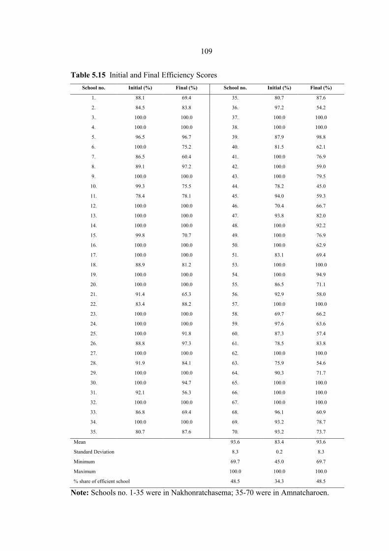
109

Table 5.15 Initial and Final Efficiency Scores

School no. Initial (%) Final (%) School no. Initial (%) Final (%)

1. 88.1 69.4 35. 80.7 87.6

2. 84.5 83.8 36. 97.2 54.2

3. 100.0 100.0 37. 100.0 100.0

4. 100.0 100.0 38. 100.0 100.0

5. 96.5 96.7 39. 87.9 98.8

6. 100.0 75.2 40. 81.5 62.1

7. 86.5 60.4 41. 100.0 76.9

8. 89.1 97.2 42. 100.0 59.0

9. 100.0 100.0 43. 100.0 79.5

10. 99.3 75.5 44. 78.2 45.0

11. 78.4 78.1 45. 94.0 59.3

12. 100.0 100.0 46. 70.4 66.7

13. 100.0 100.0 47. 93.8 82.0

14. 100.0 100.0 48. 100.0 92.2

15. 99.8 70.7 49. 100.0 76.9

16. 100.0 100.0 50. 100.0 62.9

17. 100.0 100.0 51. 83.1 69.4

18. 88.9 81.2 53. 100.0 100.0

19. 100.0 100.0 54. 100.0 94.9

20. 100.0 100.0 55. 86.5 71.1

21. 91.4 65.3 56. 92.9 58.0

22. 83.4 88.2 57. 100.0 100.0

23. 100.0 100.0 58. 69.7 66.2

24. 100.0 100.0 59. 97.6 63.6

25. 100.0 91.8 60. 87.3 57.4

26. 88.8 97.3 61. 78.5 83.8

27. 100.0 100.0 62. 100.0 100.0

28. 91.9 84.1 63. 75.9 54.6

29. 100.0 100.0 64. 90.3 71.7

30. 100.0 94.7 65. 100.0 100.0

31. 92.1 56.3 66. 100.0 100.0

32. 100.0 100.0 67. 100.0 100.0

33. 86.8 69.4 68. 96.1 60.9

34. 100.0 100.0 69. 93.2 78.7

35. 80.7 87.6 70. 93.2 73.7

Mean 93.6 83.4 93.6

Standard Deviation 8.3 0.2 8.3

Minimum 69.7 45.0 69.7

Maximum 100.0 100.0 100.0

% share of efficient school 48.5 34.3 48.5

Note: Schools no. 1-35 were in Nakhonratchasema; 35-70 were in Amnatcharoen.

110

Table 5.16 presents the application of the Bayesian stochastic frontier

analysis (BSFA) using the PETS and QSDS data in the model to compute the

efficiency scores.

Table 5.16 Efficiency Scores of BSFA

School no. TE (%) School no. TE (%) School no. TE (%) School no. TE (%)

1. 91.7 18. 92.8 35. 94.3 53. 92.7

2. 97.0 19. 96.9 36. 92.0 54. 96.9

3. 94.6 20. 89.2 37. 97.1 55. 89.1

4. 86.1 21. 95.9 38. 94.7 56. 95.9

5. 86.7 22. 92.2 39. 85.9 57. 92.2

6. 91.8 23. 92.5 40. 86.9 58. 92.3

7. 84.2 24. 93.3 41. 91.8 59. 93.1

8. 93.3 25. 93.5 42. 84.1 60. 93.4

9. 84.9 26. 92.4 43. 93.4 61. 92.4

10. 93.1 27. 96.1 44. 84.6 62. 96.2

11. 92.7 28. 93.8 45. 93.1 63. 93.6

12. 96.1 29. 92.0 46. 92.6 64. 92.0

13. 93.5 30. 91.8 47. 96.2 65. 91.9

14. 96.7 31. 90.3 48. 93.8 66. 90.5

15. 97.0 32. 93.6 49. 96.8 67. 93.6

16. 92.4 33. 95.8 50. 97.0 68. 95.8

17. 96.5 34. 87.7 51. 92.3 69. 88.0

52. 96.3 70. 94.0

Mean 92.3

Standard Deviation 0.03

Minimum 84.1

Maximum 97.1

Note: School no. 1-35 were in Nakhonratchasema; 35-70 were in Amnatcharoen.

The mean average efficiency of the BSFA was 92.3%, and the potential

savings was at about 7.7%, where the standard deviation was as little as 0.03. The

score for the school with the lowest efficiency was 84.1%, whereas the highest score

was 97.1%. This suggests that the mean efficiency variation was small. The next

section will compare the efficiency score results derived from the various techniques.

111

5.2.5 Comparison of Technical Efficiency Estimation

The school level technical efficiency estimation (i.e. DEA, SFA, posterior

means for the Bayesians specification) was generated by all of the estimation

methods. As these estimates are frequently the focus of efficiency estimation for

policymakers, it is important to see if any difference between the alternatives

methodologies can be identified. The technical efficiency estimates for a random

sample of schools as well as various summaries are reported in Table 5.17.

In general, the average estimates of technical efficiency for the various

methodologies appear to be relatively similar, except for the DEA, which was lower.

This finding is in keeping with most other comparative studies in the literature

(Balcombe, 2006: 2230). Furthermore, the results were not surprising, as Zhang and

Bartels (1998: 187-204) had shown that for larger samples the DEA average estimates

of technical efficiency is smaller.

The average level of technical efficiency from all method seems not to be

influenced by methodology; the schools in this sample group can be considered

efficient given the fixed inputs. Indeed, it is probably unrealistic to expect higher

average estimates of technical efficiency when stochastic events are allowed for

socioeconomics and the schools’ institutional arrangement, such as household

income, location, school size, etc.

112

Table 5.17 Average Efficiency Scores, DEA, SFA and BSFA

School no. DEA SFA BSFA School no. DEA SFA BSFA

1. 69.4 88.7 91.7 36. 54.2 88.9 92.0

2. 83.8 85.2 97.0 37. 100.0 98.5 97.1

3. 100.0 90.2 94.6 38. 100.0 91.3 94.7

4. 100.0 91.1 86.1 39. 98.8 90.2 85.9

5. 96.7 92.5 86.7 40. 62.1 89.4 86.9

6. 75.2 87.8 91.8 41. 76.9 92.6 91.8

7. 60.4 91.1 84.2 42. 59.0 93.2 84.1

8. 97.2 88.4 93.3 43. 79.5 90.6 93.4

9. 100.0 89.4 84.9 44. 45.0 89.2 84.6

10. 75.5 88.9 93.1 45. 59.3 91.8 93.1

11. 78.1 87.5 92.7 46. 66.7 89.5 92.6

12. 100.0 88.1 96.1 47. 82.0 91.5 96.2

13. 100.0 90.6 93.5 48. 92.2 90.2 93.8

14. 100.0 89.1 96.7 49. 76.9 89.7 96.8

15. 70.7 84.6 97.0 50. 62.9 89.6 97.0

16. 100.0 85.9 92.4 51. 69.4 89.4 92.3

17. 100.0 88.9 96.5 52. 95.9 89.9 96.3

18. 81.2 86.2 92.8 53. 100.0 98.8 92.7

19. 100.0 87.4 96.9 54. 94.9 89.1 96.9

20. 100.0 89.7 89.2 55. 71.1 89.2 89.1

21. 65.3 85.9 95.9 56. 58.0 90.1 95.9

22. 88.2 88.9 92.2 57. 100.0 87.4 92.2

23. 100.0 87.4 92.5 58. 66.2 87.8 92.3

24. 100.0 91.4 93.3 59. 63.6 91.6 93.1

25. 91.8 86.7 93.5 60. 57.4 80.3 93.4

26. 97.3 89.9 92.4 61. 83.8 90.1 92.4

27. 100.0 91.1 96.1 62. 100.0 87.8 96.2

28. 84.1 87.6 93.8 63. 54.6 88.8 93.6

29. 100.0 88.7 92.0 64. 71.7 88.9 92.0

30. 94.7 86.1 91.8 65. 100.0 89.1 91.9

31. 56.3 87.8 90.3 66. 100.0 88.3 90.5

32. 100.0 89.1 93.6 67. 100.0 90.3 93.6

33. 69.4 87.1 95.8 68. 60.9 89.8 95.8

34. 100.0 87.8 87.7 69. 78.7 89.9 88.0

35. 87.6 86.4 94.3 70. 73.7 87.5 94.0

Mean 83.4 89.3 92.3

Standard Deviation 0.2 0.02 0.03

Minimum 45.0 84.6 84.1

Maximum 100.0 98.8 97.1

Note: Schools no. 1-35 were in Nakhonratchasema; 35-70 were in Amnatcharoen.

113

The point estimation of technical efficiency can be seen by examining the

results in Table 5.18, which show the frequency distribution of technical efficiency

for all of the methods employed, and the results for each specific method.

The bottom percentile of schools for the SFA and BSFA can be identified.

These results, like those of the DEA, indicate that there were a significant number of

technically-inefficient schools in the sample. However, unlike the DEA, these schools

are part of a much narrower tail and as a result are more easily identified. However,

the identification of the best-performing school was less clear with the SFA and

BSFA, with many firms yielding a cluster ranging from 85.0% to 94.9%. As a result,

it is argued that it is easier to identify those schools that poorly performed compared

with the good performers. This result is important for applied practitioners of frontier

research; SFA and BSFA provide a strong characterization of poorly-performing

schools.

Table 5.18 Frequency Distribution of Technical Efficiency

Efficiency Score (%) DEA (Final) SFA BSFA

45.0 - 49.9 1

50.0 - 54.9 2

55.0 - 59.9 5

60.0 - 64.9 5

65.0 - 69.9 6

70.0 - 74.9 4

75.0 - 79.9 7

80.0 - 84.9 5 2 4

85.0 - 89.9 2 47 8

90.0 - 94.9 4 19 40

95.0 - 100.0 29 2 18

The results generated by the estimation methods were examined, by

performing a simple t-test on the difference between samples means for paired data.

It was found that there were significant differences at the 1% level for each paired.

This suggests that these methods significantly produce differently. The differences

between sample means for paired data were reported in Table 5.19.

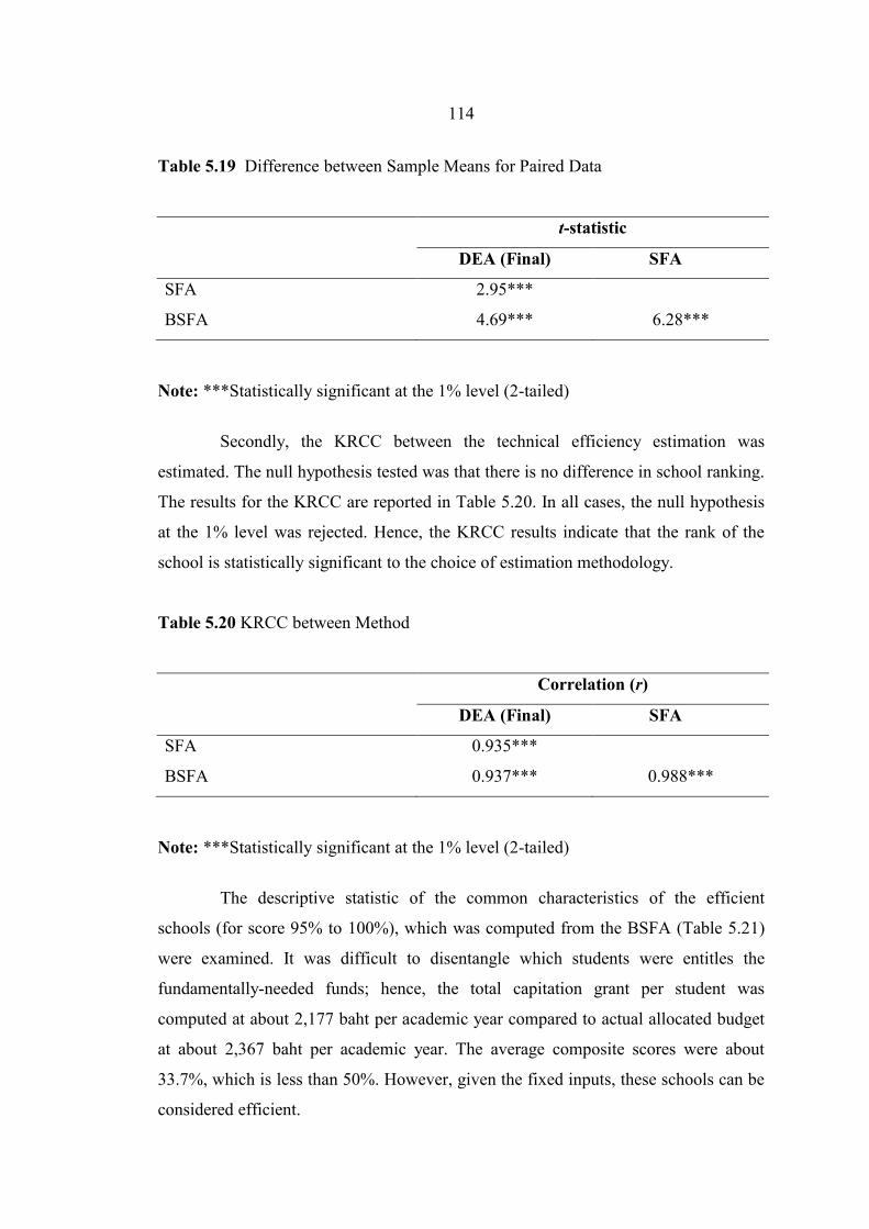
114

Table 5.19 Difference between Sample Means for Paired Data

t-statistic

DEA (Final) SFA

SFA 2.95***

BSFA 4.69*** 6.28***

Note: ***Statistically significant at the 1% level (2-tailed)

Secondly, the KRCC between the technical efficiency estimation was

estimated. The null hypothesis tested was that there is no difference in school ranking.

The results for the KRCC are reported in Table 5.20. In all cases, the null hypothesis

at the 1% level was rejected. Hence, the KRCC results indicate that the rank of the

school is statistically significant to the choice of estimation methodology.

Table 5.20 KRCC between Method

Correlation (r)

DEA (Final) SFA

SFA 0.935***

BSFA 0.937*** 0.988***

Note: ***Statistically significant at the 1% level (2-tailed)

The descriptive statistic of the common characteristics of the efficient

schools (for score 95% to 100%), which was computed from the BSFA (Table 5.21)

were examined. It was difficult to disentangle which students were entitles the

fundamentally-needed funds; hence, the total capitation grant per student was

computed at about 2,177 baht per academic year compared to actual allocated budget

at about 2,367 baht per academic year. The average composite scores were about

33.7%, which is less than 50%. However, given the fixed inputs, these schools can be

considered efficient.

115

Table 5.21 Common Characteristic of Efficient Schools

Variables Average SD Min Max

THAI (%) 40.8 6.7 32.8 57.3

MATH (%) 27.6 4.0 22.8 40.0

SCIENCE (%) 36.1 6.5 25.8 51.0

ENGLISH (%) 27.6 5.3 23.5 47.7

SOCIAL (%) 39.1 6.6 28.9 53.4

TS (%) 33.7 5.0 26.9 48.8

Funds/student/AY (Baht) 2,177 651 1,328 3,346

PROVINCE (Dummy, 0/1) 0.5 0.5 0.0 1.0

POLITICIAN (Dummy, 0/1) 0.5 0.5 0.0 1.0

ABSENT (%) 9.0 3.3 4.0 15.4

LKPERCAP (baht) 29,996 44,385 396 136,300

LKFUNDNEED (Baht) 15,852 21,353 280 64,450

HETERO (Standard deviation) 3.5 0.4 2.8 4.0

INCOME (Baht) 4,528 1,470 3,000 7,500

PARENT (Proportion, 0 to 1) 0.7 0.5 0.0 1.0

PARENTEDU (School’s year) 12.9 4.0 9.0 19.0

INSPECTION (Times) 5.6 3.1 3.0 15.0

VACANT (%) 11.1 10.2 1.0 31.8

SCHOOLSIZE (No.of student/classroom) 5.0 1.8 2.5 8.5

FEMALE (Percent of female students) 46.3 2.4 40.1 50.0

BITUMEN (Kilometer) 0.9 0.2 0.5 1.0

PARTICIPATION (Times) 0.6 0.2 0.1 0.9

Note: THAI = Average Thai languages test scores, MATH = Average Mathematics test scores,

SCIENCE = Average Sciences test scores, ENGLISH = Average English Languages test scores,

SOCIAL = Average Social Studies test scores, TS = Average five subjects scores,

Funds/student/AY = Average of capitation grants and fundamentally-needed funds per student

for academic year 2006, PROVINCE = Province dummy, POLITICIAN = Politicians’

involvement dummy, ABSENT = Teacher absence rate, LKPERCAP = Mismatch capitation

grants, LKFUNDNEED = Mismatch fundamentally-needed funds, HETERO = Heterogeneity,

INCOME = Household average income, PARENT = Living with parent, PARENTEDU = Parent’s

education, INSPECTION = Number of Inspection, VACANT =Teacher vacancy rate,

SCHOOLSIZE = School size, FEMALE = Share of female students, BITUMEN = Nearest

bitumen road, PARTICIPATION = Parent meeting with school

116

Regarding the socioeconomic and institutional factors, half of the efficient

schools were from Amnatcharoen and the others were from Nakhonratchasema. On

average, 50% of politicians supported the schools. The absence rate and vacancy rate,

which represent the management of the school, were about 9% and 11%, respectively.

The leakage of capitation grants and fundamentally-needed funds from the surveys

was about 30,000 and 16,000 baht per academic year. The household income of the

students in the efficient school was 4,530 baht per month. About 67% of students

lived with their parents. Regarding parents’ education, students in efficient schools

had the parents who received education at least nine years. Inspection was the proxy

of compact; the efficient schools received inspection about 5 times per academic year.

Regarding parents’ participation, which represents client power, the efficient schools

reported that about 57% of parents participated in school activities when called. The

characteristic of peers in efficient schools was that the share of female students was

about 46% and low variation of innate ability. School size was 20 students per

classroom and these schools had a bitumen road virtually attached to the school.

Based on analysis, BSFA seems to provide the proper school ranking.

To summarize, the above section measure of the efficiency of the sample

schools using various methods. For the data examined and the particular

specifications employed, there was a difference in the results generated by the

alternative frontier approaches. The coefficient that was significant in second stage

Tobit regression was also significant in the SFA model. The point estimate results

used in this section indicated that there was some evidence of differences between the

schools’ technical efficiency. It was also found that the SFA and BSFA results

provided a sharper distinction of technically inefficiency as opposed to technically-

efficient schools. Although the magnitude of efficiency scores was statistically

significant from zero, when the relative rank of the school using KRCC was

examined, it was found that all methods were statistically significant and close to one,

implying that the efficiency rank of schools was variant across methods. Finally, the

efficiency scores produced from the BSFA were used to describe the characteristics of

the best performing schools.

CHAPTER 6

CONCLUSION AND POLICY RECOMMENDATIONS

“The great advances of civilization, whether in architecture or painting, in

science or literature, in industry or agriculture, have never come from centralized

government.”

Milton Friedman (2002: 3)

6.1 Conclusion of the Study

This paper uses a new and primary dataset to provide a comprehensive

analysis of the impact of leakage and weak institutional capacity of schools on

compulsory school academic achievement proxied by technical efficiency in

Thailand. This analysis provides a school-based management framework as a frame of

reference of the study, and it uses efficiency measurement estimation techniques to

estimate school efficiency.

1. The leakage of public expenditures proxied by capitation grants and

fundamentally-needed funds was estimated. The findings are: for fiscal year (FY)

2006, the leakage of capitation grant was about 3.1%, and leakage of fundamentally-

needed funds was 7.3%. For FY 2007, where the leakage of capitation grants of

schools in both provinces was about 3.9%, and the schools in Amnatcharoen and

Nakhonratchasema exhibited leakages of fundamentally-needed funds at 7.2%,

respectively.

118

The average amount of leakage of all types of capitation grants of sampled

schools in Nakornratchasema and Amnatcharoen was 28,100 baht and 24,800 baht,

respectively. Overall, the average amount of leakage of all schools in AY 2006 was

5.8% or about 52,900 baht.

2. The weak institutional capacity of schools: teacher absenteeism and

budgetary allocation delays were diagnosed. The findings are: the vacancy rate in the

schools in AY2006 was 17%, with the vacant teacher position at the schools in

Amnatcharoen compared with Nakhonratchasema being higher (23% compare to 9

%). Absence rate in AY 2007 in Amnatcharoen and Nakhonratchasema was about

9%, and 4%, respectively. The overall absence rate was 6%. In addition, the survey

indicates that the schools faced related problems of teacher shortage. Regarding the

difference in actual numbers of teachers and the number of teachers supposed to be at

work, the higher the different percentage the greater the shortage. The measure is

based on a direct response from the head teachers to the question regarding whether

the school experienced a shortage of teachers for more than one semester. A 49%

teacher shortage was reported. Schools from Nakhonratchasema and Amnatcharoen

were estimated at 55%, and 40%, respectively. It is evidenced that remote areas need

not have a higher shortage of teachers. The overall average of teacher shortage was

49%. The average delay was about 7 official days, with the schools in Amnatcharoen

and Nakhonratchasema reporting disbursement delays of 8 days and 6 days,

respectively. There was a non-significant delay in the receipt of salary payments.

However, about 25% of teachers reported a compensation delay in things other than

salary, i.e. allowances they were eligible for such as bonuses and teachers’ academic

standing. The average delay (for those experiencing delays) was about 120 days.

Teachers of schools in Amnatcharoen and Nakhonratchasema reported delays of 38%

and 13%, respectively.

The correlation of teacher absence and leakage was analyzed. The

inadequacy of school infrastructure promoted teacher absence rate at a 15%

significant level. It is imply that a more favorable school operating environment

promotes teacher presence. The results showed that teachers do not report to work if

there is an inadequate school infrastructure. Regression analysis was employed to

explore the correlation of leakage (capitation grants and fundamentally–needed funds)

119

to institutional arrangements for AY 2006. The findings are: there was a significant

difference between the provinces. Schools in Amnatcharoen seemed to have higher

leakage. Teacher absence rate was associated with leakage. This implies that the

higher the teacher absence rate, the higher the leakage of capitation grants.

Specification I exhibits another significant contributing factor, which was teacher

experience. The school that has the more experienced teachers tends to have a reduced

leakage effect. The results look different for fundamentally-needed funds. Payment

delays that are statistically significant correlate with leakage. However, specification

II implies that the province dummy was not significant in the model, and only

payment delay statistically and significantly explained the leakage. For specification

III, the factor that significantly explained the leakage of fundamentally-needed fund

was similar to specification I. Based on the analysis, specification I-III confirmed that

payment delays are an important contributing factor that promotes leakage.

3. School technical efficiency was measured in order to explain the factors

that influence efficiency empirically, based on the survey. The findings are: the results

of school technical efficiency using the data envelopment analysis (DEA), where only

quantitative factors were included; the share of efficient schools was 37.1% when

CRS was assumed and 48.5% when VRS was assumed. The average efficiency of

schools was 87.4% assuming CRS, indicating an average savings potential of 12.6%

in the use of resources. The average efficiency of schools was 93.6% assuming VRS,

and a potential savings of 6.4%. Consider how efficiency is associated with some of

the variables of interest. The results of the model assuming CRS in specification I:

leakage of capitation grants, leakage of fundamentally-needed funds, and

heterogeneity can significantly explain inefficiency; however, heterogeneity seems to

reduce inefficiency. For specification II, leakage of the fundamentally-needed and

vacancy rate promotes inefficiency; however, if a school is located near a bitumen

road, this promotes efficiency. The school that has lack of teachers in a particular

subject may affect student achievement. The comparison between schools from both

provinces seems to be significantly different: schools in Nakhonratchasema perform

more efficiently.

The same data were employed to analyze the efficiency of the school using

the stochastic frontier analysis (SFA). The findings are: the politicians’ involvement

120

variable in the stochastic part was negative and significant, which implies that

inefficiency decreases when politicians support schools. The socioeconomic variable

coefficients, such as household income, increase efficiency; however, the coefficient

on institutional variables, including leakage of capitation grants and teacher vacant

rate, promote inefficiency. It should be noted that students from the high income

households promote efficiency, giving other things equal. The variable that exhibited

an efficiency increasing effect was inspection, bigger school-size, a nearby bitumen

road. Surprisingly, the coefficients on parental participation were significant and

positive to inefficiency, suggesting that inefficiency increases due to an increase in

these factors. The cross elasticities of substitution exhibited an average positive

substitution elasticity, indicating the complement relationship-inputs needed to be

increased together in order to raise total production. The overall mean technical

efficiency (TE) was 89.3%, implying that there were possibilities to save 10.7% of

inputs usage given the production education output. The efficiency scores of the

schools that performed best were at 98.8%, and the lowest 84.6%. The high technical

efficiency scores indicated that only little output was sacrificed to inefficiency. Based

on the results there were only 2 schools that had scores ranging from 95% to 100%,

and 66 schools had scores ranging from 85%to 94.9 %. It can be seen that our sample

schools were operated under an intensive system, and that there was great potential

for increasing education production through improvements in technical efficiency.

The adjusted efficiency scores using the three-stage approach was employed.

The mean average efficiency of the VRS was 93.6% compared to the VRS (Final

result) 83.4%, where the potential savings was 16.6%. The efficiency scores were

lower than the non-parametric approach. Consequently, the share of efficient schools

decreased, the initial efficient school was 48.5% and the final result was 34.3 %. The

schools from Nakhonratchasema seemed stable in their operating environment and

extenuating circumstances, since only few schools had the reduced-scores. For school

number 6, efficiency scores were reduced from 100% to 75.2%, and for school

number 25, efficiency scores were reduced from 100% to 91.8%. However, the

schools from Amnatcharoen seemed volatile in their operating environment and

extenuating circumstances; the efficiency scores of schools number 41, 42, 43 48, 49,

50 and 54 were reduced from 100%. Furthermore, the standard deviation decreased

121

dramatically-the standard deviation of the initial efficiency scores was 8.3 and the

final efficiency score was 0.2. The Kendall rank correlation coefficient (KRCC) was

statistically significant from zero at a 1% level (2-tailed). Thus, schools that received

relatively high initial performance evaluations did so in relatively unfavorable

operating environments and extenuating circumstances; however, the variation was

small. The adjusting performance evaluations for variation in the operating

environment and for extenuating circumstances leveled the playing field, where no

variations in managerial performance were significant.

For Bayesian stochastic frontier analysis (BSFA), the mean average

efficiency of the BSFA was 92.3%, and the potential savings was at about 7.7%,

where the standard deviation was as little as 0.03. The score for the school with the

lowest efficiency was 84.1%, whereas the highest score was 97.1%. This suggests that

the mean efficiency variation was small.

4. The school technical efficiency was compared empirically, based on each

estimation technique. The finding are: the average estimates of technical efficiency

for SFA and BSFA appear to be relatively similar, except for the DEA, which was

lower. However, the identification of the best-performing school was less clear with

the SFA and BSFA, with many firms yielding a cluster ranging from 85.0% to 94.9%.

As a result, it is easier to identify those schools that poorly performed compared with

the good performers. This result is important for applied practitioners of frontier

research; SFA and BSFA provide a strong characterization of poorly-performing

schools. The results generated by the estimation methods were examined, by

performing a simple t-test on the difference between samples means for paired data. It

was found that there were significant differences at the 1% level for each paired. This

suggests that these methods significantly produce differently. The KRCC results

indicated that the rank of the school is statistically significant in relation to the choice

of estimation methodology.

The descriptive statistic of the common characteristics of the efficient

schools (for score 95% to 100%), which was computed from the BSFA were

examined. The total funds per student were computed at about 2,177 baht per

academic year compared to actual allocated budget at about 2,367 baht per academic

year. The average composite scores were about 33.7%, which is less than 50%.

122

However, given the fixed inputs, these schools can be considered efficient. Regarding

the socioeconomic and institutional factors, half of the efficient schools were from

Amnatcharoen and the others were from Nakhonratchasema. On average, 50% of

politicians supported the schools. The absence rate and vacancy rate, which represent

the management of the school, were about 9% and 11%, respectively. The leakage of

capitation grants and fundamentally-needed funds from the surveys was about 30,000

and 16,000 baht per academic year. The household income of the students in the

efficient school was 4,530 baht per month. About 67% of students lived with their

parents. Regarding parents’ education, students in efficient schools had the parents

who received education at least nine years. Inspection was the proxy of compact; the

efficient schools received inspection about 5 times per academic year. Regarding

parents’ participation, which represents client power, the efficient schools reported

that about 57% of parents participated in school activities when called. The

characteristic of peers in efficient schools was that the share of female students was

about 46% and low variation of innate ability. School size was 20 students per

classroom and these schools had a bitumen road virtually attached to the school.

Based on the analysis, the BSFA seems to provide the correct school ranking.

6.2 Policy Recommendation

The accountability relationship in the specific context of compulsory

education services, as sketched in section 3.1.4 was used to interpret the results.

According to this framework, the direct “market link” of accountability of schools

(i.e. service providers) for parents/students (client) was not strong because the system

heavily subsidized basic education. However, there was also a role for more “non-

market” direct links between clients and providers through parents’ participation.

Based on the analysis, the study results suggest some key policy

recommendations, as follows.

123

1. In order to reduce the leakage of capitation grants, schools have to

reduce the teacher absence rate. However, inadequacy of school infrastructure is

associated with absence rate. Hence, other things being equal, invest in school

infrastructure will indirectly reduce leakage. Another contributing factor that could

reduce leakage was teacher experience. This suggests the role of the government in

retaining the teacher in the school, and limiting the number of teachers in the early-

retirement program.

2. In order to reduce the leakage of fundamentally-needed funds, the school

has to reduce compensation delays such as creating the on-time payment system in

the school payroll. The leakage of two provinces was significantly different,

suggesting that distance from the central government was an important factor.

Government intervention, such as regular inspections from the central government,

invest in communication system, could address this issue.

3. In order to enhance the schools’ efficiency, school needs to prevent the

leakage of capitation grants and fundamentally-needed funds. However, regarding to

another specification, the government needs to prevent the leakage of capitation

grants, solve the vacancy rate, and built the bitumen road connected to the school. The

evidence suggests the government for recruiting new officers, and allocates more

expenditure for building bitumen roads. Alternatively, SFA yield different results. The

inefficiency function suggesting that vacancy rate had an inefficient reducing effect.

This suggests the role of the government in filling in the teacher’s vacancy. The

bigger-size schools exhibited induced efficiency; the analysis showed that the

optimum size was about 20 students per classroom. The nearest bitumen road was an

important factor in school efficiency, suggesting the same recommendations as in the

Tobit model. Surprisingly, parental participation and leakage were positive and

significant in explaining efficiency; this suggests that the government should facilitate

the parents’ participation in order to enhance student achievement and not just have

regular meetings. Inspection was a factor that the government could easily deal with in

practice, and it was recommended that the respective authorities should frequently and

officially visit the school. Regarding the socioeconomic factor, household income was

seen to promote efficiency. This implies that government subsidies alone are not

sufficient in enhancing school efficiency. Leakage of capitation was also significantly

124

associated with school efficiency; the higher the leakage, the higher the inefficiency

and it is recommended that the government lessen the leakage.

4. The BSFA the characteristic of the best performance from the worst. In

order to shift the school closer to the frontier, the analysis showed that schools should

keep up with best performer characteristics. For example, they received most of the

allocated budget (2,177 baht/student/AY), were regularly inspected by respective

authorities (6 times/AY), had a low teacher vacancy rate (11%), and appropriate

school size 25 students per classroom. However, the investment in school inputs alone

may not increase school efficiency, as the co-producer in education production; that is,

socioeconomic factors and the community, may also be important. The characteristics

of efficient schools include: average household income (4,528 baht/month) and an

existing nearest bitumen road (0.86 kilometer) etc.

6.3 Implications for the Future Research

1. This paper included only lower secondary schools in the analysis and

represents a case study of two provinces in the northeastern part of Thailand. Future

research may include broader types of public schools within the OBEC administration

and more coverage in order to obtain more data.

2. Recently, some of the schools were transferred to LAOs, and future

research may compare the efficiency of education administration between the

homogeneous types of school of ESAs compared with LAOs. The new framework,

however, would create opportunity to conduct empirical testing for robustness.

3. The multi-angular data collection technique provides the researcher with

ample data, and allows the researcher to employ other econometric models in the

analysis, thus allowing for the comparison of results and interpretations.

BIBLIOGRAPHY

Ablo, Emmanuel and Reinikka, Ritva. 1998. Do Budgets Really Matter? Evidence

from Public Spending on Education and Health in Uganda. In Policy

Research. Working Paper 1926. Washington D.C.: World Bank. Pp. 1-

35.

Ahmad, Munir and Bravo-Ureta, Boris. 1996. Technical Efficiency Measures for

Dairy Farms Using Panel Data: A Comparison of Alternative Model

Specifications. Journal of Productivity Analysis. 7(4): 399-415.

Aigner, Dennis and Chu, George. 1968. On Estimating the Industry Production

Function. American Economic Review. 58(4): 826–839.

Atagi, Rie. 2002. The Thailand Educational Reform Project: School Reform

Policy. Paper Presented to the ADB and ONEC, May.

Banker, Rajiv. D.; Charnes, Abraham and Cooper, William W. 1984. Some Models

for Estimating Technical and Scale Inefficiencies in Data Envelopment

Analysis. Management Science. 30(9): 1078-1092.

Balcombe, Kelvin; Fraser, Iain and Kim, Jae. 2006. Estimating Technical Efficiency

of Australian Dairy Farms Using Alternative Frontier Methodologies.

Applied Economics. 38(19): 2221-2236.

Bardhan, Pranab. 2002. Decentralization of Governance and Development. Journal

of Economic Perspectives. 16(4): 185-205.

Bardhan, Pranab. 2006. Decentralization and Accountability in Infrastructure

Delivery in Developing Countries. Economic Journal. 116(1): 101-127.

Bardhan, Pranab and Mookherjee, Dilp. 2000. Capture and Governance at the Local

and National Levels. American Economic Review. 90(2): 135-139.

Barrera-Osorio, Felipe; Fasih, Tazeen; Patrinos, Harry and Santibanez, Lucrecia.

2009. Decentralized Decision-Making in Schools: The Theory and

Evidence on School-Based Management. Washington, D.C.: World

Bank.

126

Bates, John. 1997. Measuring Predetermined Socioeconomic ‘Inputs’ When

Assessing the Efficiency of Educational Outputs. Applied Economics.

29(1): 85-93.

Battese, George and Coelli, Timothy. 1992. Frontier Production Functions,

Technical Efficiency, and Panel Data with Application to Paddy Farmers

in India. Journal of Productivity Analysis. 3(1-2): 153-169.

Baumol, William J. 1964. Baumol’s Sales Maximization Model: Reply. American

Economic Review. 64(December): 1081.

Bera, Anil and Sharma, Subhash. 1999. Estimating Production Uncertainty in

Stochastic Frontier Production Function Models. Journal of

Productivity Analysis. 12(3): 187–210.

Bessent, Authella; Bessent, Wailand; Kennington, Jeffery and Reagan, Billy. 1982.

An Application of Mathematic Programing to Access productivity in The

Houston Independent School District. Management Science. 28(12):

1355-1367.

Blair, Harry. 2000. Participation and Accountability at the Periphery: Democratic

Local Governance in Six Countries. World Development. 28 (1): 21-39.

BonesrØnning, Han and RattsØ, JØrn. 1994. Efficiency Variation Among The

Norwegion High Schools: Consequences of Equalization Policy.

Education of Economic Review. 13(4): 289-304.

Chakraborty, Kalyan. 2009. Efficiency in Public Education: The Role of

Socioeconomic Variables. Research in Applied Economics. 1(1): E5.

Chakraborty, Kalyan; Biswas, Basudeb and Lewis, Cris. 2001. Measurment of

Technical Efficiency in Public Education: A Stochastic and Nonstochastic

Production Frontier Approach. Southern Economic Journal. 67(4): 889-

905.

Chaudhury, Nazmul; Hammer, Jeffrey; Muralidharan, Karthik; Kremer, Michael and

Rogers, Halsey. 2003. Teacher and Health Care Provider

Absenteeism: A Multi-Country Study. Washington, D.C.: World Bank.

127

Charnes, Abraham; Cooper, William; and Rhodes, Edwardo. 1981. Evaluating

Program and Managerial Efficiency: An Application of Data Envelopment

Analysis to Program Follow Through. Management Science. 27(6): 668-

697.

Christensen, Laurits; Jorgenson, Dale, and Lau, Lawrence. 1973. Transcendental

Logarithmic Production Frontier. The Review of Economics and

Statistics. 55(1): 28-45.

Coase, Ronald. 1984. The New Institutional Economics. Journal of Institutional

and Theoretical Economics. 140(2): 229-231.

Coelli, Timothy J.; Rao, Prasada D.S.; O’Donnell, Christopher J. and Battese, George

E. 2005. An Introduction to Efficiency and Productivity Analysis.

New York: Springer.

Daraporn Dechpolmat. 2005. Efficiency Evaluation of 527 Municipalities with

Data Envelopment Analysis Techniques (DEA). Master’s thesis,

Thammasat University. (In Thai)

Das, Jishnu; Dercon, Stefan; Habyarimana, James and Krishnan, Pramila. 2004.

Teacher Shocks and Student Learning: Evidence from Zambia. Policy

Research Working Paper 3602. Washington, D.C.: World Bank.

Das, Jishnu; Dercon, Stefan; Habyarimana, James and Krishnan, Pramila. 2005a.

When Can School Inputs Improve Test Scores. Policy Research

Working Paper 3217. Washington, D.C.: World Bank.

Das, Jishnu; Dercon, Stefan; Habyarimana, James and Krishnan, Pramila. 2005b.

Public and Private Funding Basic Education in Zambia: Implications

of Budgetary Allocations for Service Delivery. Africa Region Human

Development Working Paper Series No. 62. Washington, D.C.: World

Bank.

Debreu, Gerard. 1951. The Coefficient of Resource Utilization. Econometrica.

19(3): 273–292.

Deller, Steven and Rudnicki, Edward. 1993. Production Efficiency in Elementary

Education: The Case of Maine Public Schools. Economics of Education

Review. 12: 45- 57.

128

Duncombe, William; Miner, Jerry and Ruggiero, John. 1997. Empirical Evaluation

of Bureaucratic Models of Inefficiency. Public Choice. 93(1-2): 1-18.

Engert, Frank. 1996. The Reporting of School District Efficiency: The Adequacy of

Ratio Measures. Public Budgeting and Financial Management. 8:247-

271.

Farrell, M. J. 1957. The Measurement of Productive Efficiency. Journal of the

Royal Statistical Society, Series A, General . 120(3): 253–282.

Fofack, Hippolyte; Obidegwn, Chukwuma and Ngong, Robert. 2003. Public

Expenditure Performance in Rwanda: Evidence from Public

Expenditure Tracking Surveys in Health and Education Sectors.

Africa Region Working Paper No. 45. Washington, D.C.: World Bank.

Fried, Harold; Lovell, Knox and Schmidt, Shelton. 2008. The Measurement of

Productive Efficiency and Productivity Growth. New York: Oxford

University Press.

Friedman, Milton. 2002. Capitalism and Freedom. Chicago: The University of

Chicago Press.

Fry, Gerald W. 2002. The Evolution of Educational Reform in Thailand. Paper

Presented at the Second International Forum on Education Reform: Key

Factors in Effective Implementation, September 2-5.

Gauthier, Bernard. 2006. PETS-QSDS in Sub-Saharan Africa: A Stocktaking

Study. HEC Montreal: Institute of Applied Economics.

Gauthier, Bernard and Reinikka, Ritva. 2007. Methodological Approaches to the

Study of Institutions and Service Delivery: A Review of PETS, QSDS,

and CRCS. Framework paper for the AERC Collaborative Research

Project on Institutions and Service Delivery.

Gibson, John. 2000. Who’s Not in School? Economic Barriers to Universal Primary

Education in PNG. Pacific Economic Bulletin. 15(2): 1-24.

Glewwe, Paul and Michael Kremer. 2006. Schools, Teachers, and Education

Outcomes in Developing Countries. In Handbook of the Economics of

Education . Vol 2. Eric A. Hanushek and FinishWelch, eds.

Amsterdam: Elsevier. Pp. 945-1017.

129

Gropello, Emmanuel. 2004. Education Decentralization and Accountability

Relationships in Latin America. Policy Research Working Paper 3453.

Washington D.C: World Bank.

Hanushek, Eric. 1986. The Economic of Schooling: Production and Efficiency in

Public Schools. Journal of Economic Literature. 24(3): 1141-1177.

Hanushek, Eric. 2003. The Failure of Input Based Schooling Policies. The

Economic Journal. 113(485): F64-F98.

Heidenheimer, Arnold J. and Johnston, Michael. 2009. Political Corruption.

Concepts and Contexts. 5th

ed. New Brunswick, NJ: Transaction

Publishers.

Horrace, William and Schmidt, Peter. 1996. Confidence Statements for Efficiency

Estimates from Stochastic Frontier Models. Journal of Productivity

Analysis. 7(3): 257–282.

Jondrow, James; Lovell, Knox; Materov, Ivan and Schmidt, Peter. 1982. On the

Estimation of Technical Inefficiency in the Stochastic Frontier Production

Model. Journal of Econometrics. 19(2): 233–238.

Kelvin, Lord. The Internet Encyclopedia of Science. Retrieved October 10, 2009

from http://www.daviddarling.info/encyclopedia/T/Thomson.html.

Kim, Yangseon and Schmidt, Peter. 2000. A Review and Empirical Comparison of

Bayesian and Classical Approaches to Interfere on Efficiency Levels in

Stochastic Frontier Models with Panel Data. Journal of Productivity

Analysis. 14(2): 91-118.

King, Elizabeth M. and Susana, Cordeiro-Guerra. 2005. Education Reforms in East

Asia: Policy, Process, and Impact. In East Asia Decentralizes: Making

Local Government Work. Washington, D.C.: World Bank. Pp. 179-

208.

King, Janet C. 2003. The Risk of Material Nutritional Depletion and Poor Outcomes

Increases in Early or Closely Spaced Pregnancies. The Journal of

Nutrition. Retrieved February 18, 2011 from http://jn.nutrition.org/

Koop, Gary. 2003. Bayesian Econometrics. West Sussex: Wiley.

Kpundeh, Sahr. 1997. Combating Corruption: An Assessment with International

Cases. Washington, D.C.: Management System International.

130

Kumbhakar, Subal and Lovell, Knox. 2000. Stochastic Frontier Analysis.

Cambridge: Cambridge University Press.

Lucas, Robert E., Jr. 1988. On the Mechanics of Economic Development. Journal of

Monetary Economics. 22(February): 3-42.

McCarty, Therese. and Yaisawarng, Suthathip. 1993. Technical Efficiency in New

Jersey School Districts, In The Measurement of Productive Efficiency:

Techniques and Applications. Harold Fried, Knox Lovell and Shelton

Schmidt eds. New York: Oxford University Press.

Mankiw, Gregory N; Romer, David and Weil, David N. 1992. A Contribution to the

Empirics of Economic Growth. The Quarterly Journal of Economics.

107(2): 407-437.

Martin, Michael O. Mullis, Ina V.S. and Foy, Pierre. 2008a. TIMSS 2007

International Mathematics Report: Findings from IEA’s Trends in

International Mathematics and Science Study at the Fourth and

Eighth Grades. Chestnut Hill, MA: TIMSS & PIRLS International Study

Center, Boston College.

Martin, Michael O. Mullis, Ina V.S. and Foy, Pierre. 2008b. TIMSS 2007

International Sciences Report: Findings from IEA’s Trends in

International Mathematics and Science Study at the Fourth and

Eighth Grades. Chestnut Hill, MA: TIMSS & PIRLS International Study

Center, Boston College.

Martinez-Vazquez, Jorge; del Granado, Javier-Arze and Boex, Jameson. 2007.

Fighting Corruption in the Public Sector. Contributions to Economic

Analysis 284. Amsterdam: Elsevier.

Mayston, Dennis. 2003. Measuring and Managing Educational Performance.

Journal of the Operational Research Society. 54(7): 679–691.

Ministry of Education. 2004. Education in Thailand 2004. Bangkok: Amarin.

Ministry of Education. 2008. Toward a Learning Society in Thailand: An

Introduction to Education in Thailand. Bangkok: Bureau of

International Cooperation.

Mitlin, Diana. 2000. Toward More Pro-Poor Local Governments in Urban Areas.

Environment and Urbanization. 12 (1): 3-11.

131

Mishra, Aji. 2006. Persistence of Corruption: Some Theoretical Perspectives. World

Development. 34(2): 349-359.

National Institute of Educational Testing Service. 2011. National O-NET Test

Scores Analysis. Retrieved April 5, 2011 from

http://www.niets.or.th/uploadfiles/uploadfile/9/d20ff236a6b94437d483043

655786e5d.pdf

North, Douglas. 1990. Institutions, Institutional Change and Economic

Performance. Cambridge: Cambridge University Press.

O’Donnell, Chris and Coelli, Timothy. 2005. A Bayesian Approach to Imposing

Curvature on Distance Function. Journal of Econometrics. 126(2): 493-

523.

OECD. 2010. PISA 2009 Results: Executive Summary. Retrieved April 5, 2011

form http://www.oecd.org/dataoecd/34/60/46619703.pdf.

Office of the Education Council. 2008. Education in Thailand 2007. Bangkok:

Amarin Printing and Publishing.

Office of National Economic and Social Development Board. 2009. Gross

Provincial Product (2009 Edition). Retrieved April 5, 2011

http://www.nesdb.go.th/econSocial/macro/gpp_data/index.html

Osiewalski, Jacek and Steel, Mark. 1988. Numerical Tools for the Bayesian Analysis

of Stochastic Frontier Models. Journal of Productivity Analysis. 10(1):

103-117.

Peters, Guy. 1996. The Future of Governing: Four Emerging Models. Lawrence,

KS: University Press of Kansas.

Pevalin, David J. 2003. Outcomes in Childhood and Adulthood by Mother’s Age

at Birth: Evidence from the 1970 British Cohort Study. ISER.

Working Paper 2003-31. Colchester, Essex: University of Essex.

Pitt, Mark and Lee, Lung-Fei. 1981. Measurement and Sources of Technical

Inefficiency in the Indonesian Weaving Industry. Journal of

Development Economics. 9(1): 43-64.

Pritchett, Lant and Filmer, Deon. 1999. What Production Functions Really Show: A

Positive Theory of Education Expenditures. Economics of Education

Review. 18(2): 223- 239.

132

Rassouli-Currier, Susanne. 2007a. The Choice of Estimation Method and Its Effect

of Efficiency Measurement in Public Education: Stochastic Frontier vs.

Data Envelopment Analysis. The Journal of Economics. 33(1): 53-72.

Rassouli-Currier, Susanne. 2007b. Assessing the Efficiency of Oklahoma Public

Schools: A Data Envelopment Analysis. Southwestern Economics

Review. 34(1): 131-144.

Ray, Subhash C. 1991. Resource-Use Efficiency in Public Schools: A Study of

Connecticut Data. Management Science. 37(12): 1620-1628.

Renikka, Ritva and Nathanael Smith. 2004. Public Expenditure Tracking Surveys

in Education. Paris: International Institute for Education Planning,

UNESCO.

Reinikka, Ritva and Svensson, Jakob. 2004. Efficiency of Public Spending: New

Microeconomics Tools to Assess Service Delivery. In Fiscal Policy for

Development: Poverty, Reconstruction and Growth. Tony Addison

and Alan Roe, eds. Palgrave: Macmillan. Pp. 218-336.

Ruggiero, John. 1996. Efficiency of Educational Production: An Analysis of New

York School Districts. The Review of Economics and Statistics. 78(3):

499-509.

Schmidt, Peter. 1976. On the Statistical Estimation of Parametric Frontier

Production Functions: Rejoinder. Review of Economics and Statistics.

60(3): 481-482.

Schneider, Hartmut. 1999. Participatory Governance for Poverty Reduction.

Journal of International Development. 11 (4): 531-534.

Sengupta, Jati and Sfeir, Raymond. 1986. Production Frontier Estimates of Scale in

Public Education in California. Economic of Education Review. 5: 297-

307.

Shah, Anwar, ed. 2005. Public Expenditure Analysis. Washington, D.C.: World

Bank.

Smith, Peter and Mayston, Davis. 1987. Measuring Efficiency in the Public Sector.

OMEGA International Journal of Management Science. 15(3): 181-

189.

133

Sowell, Thomas. 2000. Basic Economics: A Citizen’s Guide to the Economy.

New York: Perseus Books Group.

Theunynck, Serge. 2009. School Construction Strategies for Universal Primary

Education in Africa Should Communities Be Empowered To Build

Their Schools? Washington, D.C.: World Bank.

UNESCO. 2007. EFA Global Monitoring Report 2008. Paris: Oxford University

Press.

United Nations. 2008. The Millennium Development Goals Report 2008. New

York: United Nations.

Verspoor, Adrian. et al. 2008. At the Cross Choices for Secondary Education in

Sub-Saharan Africa. Washington D.C.: World Bank.

Wang, Hung-J. and Schmidt, Peter. 2002. One-Step and Two-Step Estimation of the

Effects of Exogenous Variables on Technical Efficiency Levels. Journal

of Productivity Analysis. 18(2): 129–44.

Winsten, C.B. 1957. Discussion on Mr. Farrell’s Paper. Journal of the Royal

Statistical Society, Series A, General. 120: 282–284.

Woessmann, Ludger. 2000. Schooling Resources, Educational Institutions, and

Student Performance: The International Evidence. Kiel Working

Paper No. 983, Munich: Kiel Institute for Economic Research.

World Bank. 1997. Helping Countries Combat Corruption. The Role of the World

Bank. PREM Notes Public Sector, 4. Washington, D.C.: World Bank.

World Bank. 2003. World Development Report 2004: Making Services Work for

Poor People. Washington, D.C.: World Bank.

World Bank. 2005a. Cambodia: Public Expenditure Tracking (PETS) in

Primary Education. Washington, D.C.: World Bank.

World Bank. 2005b. Thailand Northeast Economic Development Report.

Washington, D.C.: World Bank.

World Bank. 2006. Thailand Social Monitor: Improving Secondary Education.

Bangkok: World Bank.

World Bank. 2007. World Development Indicators 2007. Washington, D.C.:

World Bank.

World Bank. 2009. The Little Data Book. Washington, D.C.: World Bank.

134

Worthington, Andrew. 2001. An Empirical Survey of Frontier Efficiency

Measurement Techniques in Education. Education Economics. 9(3):

245-268.

Wyatt, David K. 1969. The Politics of Reform in Thailand: Education in the

Reign of King Chulalongkorn. New Haven: Yale University Press.

Yuttapong Phongsakornnoppadol. 2005. Technical Efficiency Measurement of

Elementary and Secondary Schools by Data Envelopment Analysis.

Master’s thesis, Thammasat University. (In Thai)

Zellner, Arnold. 1985. Bayesian Econometrics. Econometrica. 53(2 March): 253-

269.

Zhang, Yun and Bartels, Robert. 1998. The Effect of Sample Size on the Mean

Efficiency in DEA with an Application to Electricity Distribution in

Australia, Sweden and New Zealand. Journal of Productivity Analysis.

9(3): 187-204.

APPENDICES

Appendix A: The Jackknifing Procedure

Suppose that one wants to estimate a parameter that depends on a random

quantity sample 1 2( , ,..., )nX X X X in a complicated way. For example, might be

the sample variance of X or the log sample variance. If Xi is vector valued, could be

a Pearson correlation coefficient.

Assume that have an estimator 1 2( , ,..., )n nX X X of but does not know the

probability distribution of ( )n X given . This means that one cannot estimate the

error involved in estimating by 1 2( , ,..., )n nX X X which cannot tell if it concluded

as 0 from an observed ( ) 0n X , no matter how large. More generally, one can

get a confidence interval for depending only on the observed 1 2, ,..., nX X X , or test

0 0:H just using the data 1 2, ,..., nX X X .

Methods that try to estimate the bias and variability of an estimator

1 2( , ,..., )n nX X X by using the values of ( )n X on subsamples from 1 2, ,..., nX X X are

called resampling methods. A common resampling method is the jackknife method.

The jackknife method was invented to correcting possible bias in 1 2( , ,..., )n nX X X

for small n.

Let ( )n X = 1 2( , ,..., )n nX X X be an estimator defined for samples

1 2( , ,..., )nX X X X . The ith

pseudovalue of ( )n X is

1 2 1 1 2 [ ]( ) ( , ,..., ) ( 1) (( , ,..., ) )i n n n n ips X n X X X n X X X , (A.1)

In (6.3), [ ]iX means the sample 1 2( , ,..., )nX X X X with the thi value iX deleted from

the sample, so that [ ]iX is a sample of size n-1. Note that

1 [ ]( ) ( ) ( 1)( ( ) ( ))i n n n n ips X X n X X ,

137

so that ( )ips X can be viewed as a bias-corrected version of ( )n X determined by the

trend in the estimators ( )n X from 1 [ ]( )n n iX

to ( )n X .The basic jackknife recipe is

to treat the pseudovalue ( )ips X as if they were an independent random variable with

a mean of .

If 1

1( )

n

n jjX X X

n

is the sample mean for ( ),iE X then the

pseudovalues

[ ]( ) ( 1)i i ips X nX n X X

are the same as the original values. Thus

1

1( ) ( )

n

i

i

ps X ps X Xn

and 2

1

1( ) ( )

1

n

ps i

i

V X X Xn

(A.2)

are the usual sample mean and variance.

If 2

1

1( ) ( )

1

n

n jjX X X

n

is the sample variance, then the pseudovalues

of ( )n X are

2 2

1

1( ) ( ) ( )

2 ( 1)( 2)

n

i i j

i

nps X X X X X

n n n

, (A.3)

The mean of the pseudovalue

2

1 1

1 1( ) ( ) ( )

1

n n

i j

i j

ps X ps X X Xn n

is the same as ( )n X in this case also.

If 2

1

1( ) ( )

n

n jjX X X

n

is the sample variance with 1/(n-1) replaced by

1/n, then the pseudovalues of ( )n X are

2

1

( ) ( )1

n

i j

j

nps X X X

n

, (A.4)

138

This implies that

2

1 1

1 1( ) ( ) ( )

1

n n

i i

i i

ps X ps X X Xn n

is the usual sample variance. Note that 21

( ( ))n

nE X

n

for

2 ( )Var X ,

while2( ( ))E ps X , so that ps(X) is a bias-corrected version of ( )n X .

Appendix B: The Three-stage Approach

Stage 1 The initial DEA school evaluation

The initial school performance evaluation was already conducted using

conventional output-orientated DEA analysis. For producer “i” the VRS envelopment

problem could be expressed as a linear programming problem. However, actual

performances were likely to be attributable to some combination of managerial

inefficiencies, environment effects, and statistical noise, and it was desirable to isolate

the three effects. This could not be accomplished within the framework of the above

problem, from which the environmental variables and statistical noise were both

missing. Table B.1 presents information on output slacks.

Stage 2: Using SFA/ Tobit to Decompose Slacks

Slacks represent amounts of excessive inputs use. It reveals the extent to

which use of particular inputs can be reduced given that a school has already reached

the frontier of the production set. The output slacks was regressed against observable

fix environment variables. Composed error term where both captured and

distinguished the effects of managerial inefficiency and statistical noise. The virtue of

using SFA was that its error term was asymmetric. Consequently it allows for the

impact on the stage 1 slack of environmental variables (the regressors) of managerial

inefficiency (the one-sided error component) and of statistical noise (the symmetric

error components). Since the Stage 1 model is output-orientated, use of N Stage 1

output slacks concerns whether to estimate N separate SFA regressions, one for each

Stage 1 output slack. Then estimation of N separate SFA regressions can be chosen.

140

Table B.1 Technical Efficiency (TE) and Each Output Slacks

School no. TE Output Slacks

PG FF SA EXP CS

1. 88.1 1.91 0.00 2.97 5.42 0.00

2. 84.5 2.24 0.37 2.81 0.00 0.00

3. 100.0 0.00 0.00 0.00 0.00 0.00

4. 100.0 0.00 0.00 0.00 0.00 0.00

5. 96.5 0.00 0.00 1.01 2.94 0.00

6. 100.0 0.00 0.00 0.00 0.00 0.00

7. 86.5 6.49 8.08 0.00 7.11 2.44

8. 89.1 0.00 1.79 0.00 3.51 0.00

9. 100.0 0.00 0.00 0.00 0.00 0.00

10. 99.3 0.00 0.00 0.00 4.24 0.00

11. 78.4 0.32 0.00 0.00 0.74 0.00

12. 100.0 0.00 0.00 0.00 0.00 0.00

13. 100.0 0.00 0.00 0.00 0.00 0.00

14. 100.0 0.00 0.00 0.00 0.00 0.00

15. 99.8 0.00 3.54 0.00 0.00 0.00

16. 100.0 0.00 0.00 0.00 0.00 0.00

17. 100.0 0.00 0.00 0.00 0.00 0.00

18. 88.9 6.09 0.00 3.06 0.00 0.00

19. 100.0 0.00 0.00 0.00 0.00 0.00

20. 100.0 0.00 0.00 0.00 0.00 0.00

21. 91.4 0.00 3.74 0.00 3.19 0.00

22. 83.4 0.00 3.27 0.00 0.52 0.00

23. 100.0 0.00 0.00 0.00 0.00 0.00

24. 100.0 0.00 0.00 0.00 0.00 0.00

25. 100.0 0.00 0.00 0.00 0.00 0.00

26. 88.8 0.00 1.21 1.31 0.82 0.00

27. 100.0 0.00 0.00 0.00 0.00 0.00

28. 91.9 0.00 3.16 0.00 0.81 0.00

29. 100.0 0.00 0.00 0.00 0.00 0.00

30. 100.0 0.00 0.00 0.00 0.00 0.00

31. 92.1 0.00 4.53 0.63 10.94 0.00

32. 100.0 0.00 0.00 0.00 0.00 0.00

33. 86.8 0.00 4.60 0.00 5.83 0.00

34. 100.0 0.00 0.00 0.00 0.00 0.00

35. 80.7 0.00 2.30 3.97 0.00 0.00

36. 97.2 0.00 3.51 0.84 36. 97.2

37. 100.0 0.15 0.00 0.00 37. 100.0

38. 100.0 0.00 0.00 0.00 38. 100.0

39. 87.9 0.00 1.19 0.00 39. 87.9

40. 81.5 0.00 0.00 9.92 40. 81.5

41. 100.0 0.00 0.00 0.00 41. 100.0

141

Table B.1 (Continued)

School no. TE Output Slacks

PG FF SA EXP CS

42. 100.0 0.00 0.00 0.00 42. 100.0

43. 100.0 0.00 0.00 0.00 43. 100.0

44. 78.6 0.00 1.19 3.59 44. 78.6

45. 94.0 0.00 7.95 1.39 45. 94.0

46. 70.4 0.00 3.69 4.88 46. 70.4

47. 93.8 1.06 2.45 0.00 47. 93.8

48. 100.0 0.00 0.00 0.00 48. 100.0

49. 96.1 2.74 0.00 0.00 49. 96.1

50. 100.0 0.00 0.00 0.00 50. 100.0

51. 83.1 0.00 0.00 0.00 51. 83.1

52. 79.6 0.00 0.00 2.32 52. 79.6

53. 100.0 0.00 0.00 0.00 53. 100.0

54. 100.0 0.00 0.00 0.00 54. 100.0

55. 86.5 0.00 2.14 0.74 55. 86.5

56. 92.9 0.00 6.07 0.00 56. 92.9

57. 100.0 0.00 0.00 0.00 57. 100.0

58. 69.7 0.00 0.00 2.95 58. 69.7

59. 97.6 0.75 0.00 4.08 59. 97.6

60. 87.3 5.81 4.34 8.48 60. 87.3

61. 78.5 0.93 4.03 0.00 61. 78.5

62. 100.0 0.00 0.00 0.00 62. 100.0

63. 75.9 0.00 0.17 0.00 63. 75.9

64. 90.3 9.00 8.22 0.00 64. 90.3

65. 100.0 0.00 0.00 0.00 65. 100.0

66. 100.0 0.00 0.00 0.00 66. 100.0

67. 100.0 0.00 0.00 0.00 67. 100.0

68. 96.1 2.74 0.00 0.00 68. 96.1

69. 93.2 0.67 6.10 0.00 69. 93.2

70. 93.2 6.15 0.00 4.76 70. 93.2

Mean 93.6 0.67 1.25 0.85 2.16 0.14

Std. Dev. 8.3 1.81 2.20 1.93 3.80 0.47

Min 69.7 0.00 0.00 0.00 0.00 0.00

Max 100.0 9.00 8.22 9.92 15.74 2.44

% of school efficiency 48.5

The dependent variables in the Stage 2 SFA regression model were the Stage

1 total output slacks 0, 1,..., , 1,...,ni ni ns y Y n N i I , where nis was the Stage 1

142

nth output for the i-th school, nY was the nth row of Y, and nY was the optimal

projection of niy onto the output efficient subset for input vector ix . The independent

variables in the Stage 2 SFA regression model were comprised of the elements of the

K observable fix environmental variables, 1[ ,..., ], 1,..., .i i Kiz z z i I The N separate

Stage 2 SFA regressions took the general form:

( ; ) ,n n

ni i ni nis f z v u 1,..., , 1,...,n N i I , (B.1)

where the ( ; )n n

if z was the deterministic feasible slack frontier with parameter

vector n to be estimated and composed error structure, ( ni niv u ). Assume that the

2(0, )ni vnv N reflected statistical noise and that the 0niu reflected managerial

inefficiency. If 2( , ),n

ni unu N and we assume that the niv and the niu were

distributed independently of each other, and of the iz , each of the N regressions (B.1)

may be estimated by maximum likelihood techniques. In each regression the

parameters to be estimated were 2 2( , , , ).n n

vn un All parameters were allowed to

vary across the N output slack regressions, which allows the environmental variables,

statistical noise, and managerial inefficiency each to exert a different impact across

outputs.

The impact of the environment on Stage 1 slacks was captured by the

deterministic feasible slacks frontiers ( ; )n n

if z . However, this relationship was

noisy, and so the stochastic feasible slack frontiers (SFSF) were [ ( ; ) ]n n

i nif z v .

Since 0niu , this represents the maximum slacks that can be achieved in a noisy

environment ( , )i niz v and parameter 2( , )n

vn . Any slacks less than the SFSF are

attributable to managerial inefficiency because the effects of both the environmental

variables iz and statistical noise niv were netted out, having been captured by the

SFSF. The managerial inefficiency component of the slacks was captured by the

nonnegative error components ,niu with parameters 2( , )n

un reflecting the variability

of managerial inefficiency, both across schools and across outputs.

143

The essence of the proposed adjustment exploits the fact that schools

operating in relatively unfavorable environments, and schools experiencing relatively

bad luck, were disadvantaged in the Stage 1 DEA performance evaluation and did not

take these factors into account. The extent to which they have been disadvantaged by

each source was revealed by the parameter estimates obtained in the Stage 2 SFA

regressions. The analysis adjusts upward of outputs of schools that had an advantage

because of their relatively favorable operation or because of their relatively good luck.

This approach can avoid the possibility that some extremely disadvantaged schools

might have some inputs adjusted so far downward as to become negative. Following

Chakarborty (2009: 9), the author assumed ( ; )n n

if z , was assumed in the semilog,

where the dependent variables was the natural logarithm and could estimate the

coefficient of the independent variables in the Stage 2 SFA:

0 1 2 3 4( )niLn s PROVINCE POLITICIAN ABSENT MISPERCAP

+ 5 6 7 8MISFUNDNEED HETERO INCOME PARENTS

+ 9 10 11 12PARENTEDU INSPECTION VACANT SCHOOLSIZE

+ 13 14 15 iFEMALE BITUMEN PARTICIPATION . (B.2)

The results from the stochastic production frontier model and inefficiency

effects model are reported in Table B.2. A likelihood ratio test was not able to reject

the hypothesis that the one-sided error component makes no contribution to the error

term, in which the stochastic frontier specification was rejected. This suggests that

variation in managerial inefficiency plays no role in this output. Consequently, the

parameter estimates for further use for output slacks were based upon a Tobit

specification since the slacks computed from the DEA model were truncated from

below at zero; an OLS regression would produce biased and inconsistent parameter

estimates. The model is specified as follows:

n

ni ni nis r v if 0nis , (B.3)

= 0

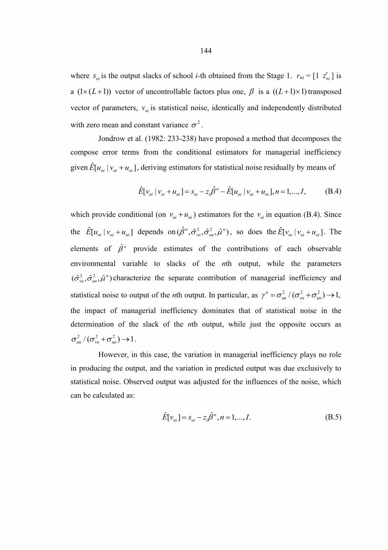
144

where nis is the output slacks of school i-th obtained from the Stage 1. rni = [1 niz ] is

a (1 ( 1))L vector of uncontrollable factors plus one, is a (( 1) 1)L transposed

vector of parameters, niv is statistical noise, identically and independently distributed

with zero mean and constant variance 2 .

Jondrow et al. (1982: 233-238) have proposed a method that decomposes the

compose error terms from the conditional estimators for managerial inefficiency

given ˆ[ | ]ni ni niE u v u , deriving estimators for statistical noise residually by means of

ˆˆ ˆ[ | ] [ | ], 1,..., ,n

ni ni ni ni i ni ni niE v v u s z E u v u n I (B.4)

which provide conditional (on ni niv u ) estimators for the niv in equation (B.4). Since

the ˆ[ | ]ni ni niE u v u depends on 2 2ˆ ˆ ˆ ˆ( , , , )n n

vn un , so does the ˆ[ | ]ni ni niE v v u . The

elements of ˆ n provide estimates of the contributions of each observable

environmental variable to slacks of the nth output, while the parameters

2 2ˆ ˆ ˆ( , , )n

vn un characterize the separate contribution of managerial inefficiency and

statistical noise to output of the nth output. In particular, as 2 2 2/ ( ) 1,n

un vn un

the impact of managerial inefficiency dominates that of statistical noise in the

determination of the slack of the nth output, while just the opposite occurs as

2 2 2/ ( ) 1un vn un .

However, in this case, the variation in managerial inefficiency plays no role

in producing the output, and the variation in predicted output was due exclusively to

statistical noise. Observed output was adjusted for the influences of the noise, which

can be calculated as:

ˆˆ[ ] , 1,..., .n

ni ni iE v s z n I

(B.5)

145

Table B.2 Stochastic Frontier Estimate Results

Dependent Variables-Slack

Variables PG FF SA EXP CS

Intercept 2.35 -0.79 4.83 -4.54 0.36

(2.35) (0.79) (0.90) (0.53) (0.36)

PROVINCE 0.56 0.76 0.99 1.79 0.11

(0.56) (0.76) (2.15) (2.08) (0.11)

POLITICIAN 0.44 0.06 0.63 -0.57 0.27

(0.44) (0.06) (1.27) (0.65) 0.27)

ABSENT -0.002 0.04 -0.03 0.14 0.04

(0.002) (0.04) (0.50) (1.17) (0.04)

LKPERCAP -0.000003 -0.00000004 -0.000002 0.00002 -0.00000003

(0.000003) (0.00000004) (0.36) (2.05) (0.00000003)

LKFUNDNEED -0.000005 0.000001 -0.00001 0.0000004 0.0000007

(0.000005) (0.000001) (1.13) (0.02) (0.0000007)

HETERO -0.38 0.19 -0.21 -0.80 -0.05

(0.38) (0.19) (0.40) (0.86) (0.05)

INCOME -0.00003 -0.0002 -0.00003 -0.0006 -0.00007

(0.00003) (0.0002) (0.12) (1.62) (0.00007)

PARENT -0.19 0.17 0.58 0.78 0.11

(0.19) (0.17) (1.25) (0.92) (0.11)

PARENTEDU -0.02 -0.17 -0.09 -0.13 -0.008

(0.02) (0.17) (1.18) (0.93) (0.008)

INSPECTION -0.003 -0.09 0.006 0.14 -0.003

(0.003) (0.09) (0.10) (1.45) (0.003)

VACANT 0.03 0.03 0.03 0.06 -0.01

(0.03) (0.03) (0.96) (1.14) (0.01)

SCHOOLSIZE -0.03 0.0002 -0.03 -0.07 -0.01

(0.03) (0.0002) 1.05 (1.20) (0.01)

FEMALE 0.008 0.11 -0.05 0.21 -0.0005

(0.008) (0.11) (0.63) (1.49) (0.0005)

BITUMEN -0.08 -0.11 -0.07 -0.24 0.007

(0.08) (0.11) 1.05 (1.90) (0.007)

PARTICIPATION -0.16 -1.73 0.10 0.65 -0.01

(0.16) (1.73) (0.09) (2.93) (0.01)

2 3.06 3.80 3.09 10.45 0.17

(3.06) (3.80) (6.05) (6.11) (0.17)

0.05 0.05 0.000006 0.0000004 0.05

(0.05) (0.05) (0.0007) (0.0009 (0.05)

Log-likelihood function -137.38 -144.97 -138.96 -181.47 -356.24

LR test - - - - -

Note: t-stat in parenthesis

146

Note that ˆ[ ]niE v is not bounded from below at zero; it can take on negative,

zero, or positive values. If ˆ[ ]niE v is zero, then the school performs as well as the

average school with the same set of uncontrollable factors. If ˆ[ ]niE v is not equal to

zero, then its performance differs from the average school with the same set of

uncontrollable factors. The parameter estimate for outputs slacks was based upon

Tobit specification reported in Table B.3. The results suggest that some of the

operating environments do indeed exert a statistically influence on school

performance. The teacher absence rate was significant with CS output slacks. Leakage

of capitation grants, average household income, parents’ education, teachers’ vacancy

rate, share of female students, and nearest bitumen road were significant in explaining

EXP outputs slacks.

However, no other uncontrollable inputs can explain SA output slack

(column 3). Parents’ education and teachers’ vacancy rate were significantly

correlated with FF output slacks (column 2), and only heterogeneity was associated

with PG output slacks (column 1). Schools’ adjusted outputs were constructed from

the results of the Stage 2 Tobit regressions by mean of the following:

ˆ ˆ ˆ ˆ[max ] [max ], 1,..., , 1,..., ,A n n

ni ni i i i ni niy y z z v v n N i I (B.6),

where A

niy and niy were adjusted and observed output quantities, respectively. The first

adjustment on the right side of the equation puts all schools into a common operating

environment, which is the least favorable environment. The second adjustment puts

all schools into a common state of nature, which was the unluckiest situation

encountered. Thus schools with the relatively least favorable operating environments

and/or which were relatively unluckiest had their outputs adjusted upward by a

relatively small amount, while producers with relatively favorable operating

environments and/or relatively good luck have their outputs adjusted upward by a

relatively large amount. These adjustments vary both across producers and across

outputs.

147

Table B.3 Tobit Frontier Estimate Results

Slacks Variables

Variables PG FF SA EXP CS

Intercept 9.14 -12.38 7.76 -11.78 -7.56

(0.35) (0.64) (0.39) (0.43) (0.68)

PROVINCE 3.89* 2.71* 3.14* 5.30** 1.42

(1.73) (1.55) (1.78) (2.44) (1.11)

POLITICIAN 1.92 0.77 2.64 -1.13 0.89

(0.94) (1.48) (1.48) (0.53) (1.11)

ABSENT -0.25 -0.06 -0.06 0.14 0.31*

(0.81) (0.30) (0.23) (0.50) (1.90)

LKPERCAP -0.00002 0.000006 0.0000002 0.00004** 0.000005

(0.72) (0.46) (0.02) (2.15) (0.63)

LKFUNDNEED -0.00005 0.00001 -0.00004 0.000008 0.00002

(0.81) (0.36) (0.83) (0.17) (1.04)

HETERO -4.16* -0.30 -1.52 -2.70 0.36

(1.66) (0.17) (0.74) (1.11) (0.32)

INCOME -0.0002 -0.0009 -0.0001 -0.002** -0.0004

(0.16) (1.21) (0.17) (2.04) (1.13)

PARENT -1.33 -0.61 1.65 -0.69 0.94

(0.65) (0.41) (0.99) (0.34) (1.16)

PARENTEDU -0.21 -0.65** -0.36 -0.72** -0.04

(0.63) (2.12) (1.17) (1.81) (0.31)

INSPECTION -0.11 -0.20 0.06 0.17 0.06

(0.42) (1.07) (0.30) (0.76) (0.66)

VACANT 0.07 0.16* 0.13 0.23* 0.004

(0.54) (1.69) (1.29) (1.99) (0.08)

SCHOOLSIZE -0.64 -0.02 -0.37 -0.17 -0.06

(1.07) (0.21) (0.78) (1.19) (0.82)

FEMALE 0.24 0.53 -0.06 0.67** 0.02

(0.55) (1.54) (0.19) (1.47) (0.14)

BITUMEN -0.36 -0.67 -0.24 -0.60* -0.09

(1.21) (1.37) (0.95) (1.97) (0.36)

PARTICIPATION -3.31 -4.62 1.58 -2.85 0.51

(0.63) (1.20) (0.36) (0.54) (0.23)

Log likelihood -62.31 -84.75 -72.02 -108.59 -48.04

n

70 70 70 70 70

Note: z-stat in parenthesis, *significant at the 10% and **significant at the 5% level

148

The observed outputs were adjusted for the influences of the environment

and noise by inserting the parameter estimate obtained from the Stage 2 Tobit

regression into equation (B.6). This procedure reflected variation in the operating

environment and statistical noise. It did not reflect variation in efficiency in managing

the external environment, which was negligible for each output. The outputs adjusted

are shown in Table B.4.

Table B.4 Outputs Adjustment after Stage 2

PP FF SA EXP CS

Initial Adjusted Initial Adjusted Initial Adjusted Initial Adjusted Initial Adjusted

Mean 41.46 146.78 29.42 148.77 38.52 136.20 29.16 134.49 40.44 86.29

S.D. 4.54 64.42 5.38 51.42 7.78 42.54 5.14 63.64 5.93 20.05

Min. 32.78 53.65 23.33 67.63 28.33 40.88 21.88 42.84 31.50 40.15

Max. 50.00 456.38 54.17 286.80 66.17 301.66 47.33 441.96 53.41 132.45

Stage 3: The DEA Final School Evaluation

A DEA was done again using data from the stage 2 adjusted-outputs.

Appendix C: Data on Thailand

East Asia & Pacific Lower middle income

Population (millions) 64 Population growth (%) 0.6

Surface area (1,000 sq. km) 513

National poverty rate (% of pop.) ..

GNI ($ billions) 217.2

GNI per capita ($) 3,400

GNI, PPP ($ billions) 502.8 GNI per capita, PPP ($) 7,880

1990 2000 2007

People

Share of poorest 20% in natt'l consumption/income (%) 5.6 6.2 ..

Life expectancy at birth (years) 67 68 71

Total fertility (births per woman) 2.1 1.9 1.9

Adolescent fertility (births per 1,000 woman 15-19)

.. 46 42

Contraceptive prevalence (% of married woman 15-49) .. 79 77

Births attend by skilled health staff (% of total)

.. 99 97

Under-five mortality rate (per 1,000) 31 13 7

Child malnutrition, underweight (1% of under age 5) .. .. 7.0

Child immunization, measles (% of ages 12-23 mos.) 80 94 96

Primary completion rate, total (% of relevant age group) .. 96 101

Gross secondary enrollment, total (% of relevant age group) 30 67 83

Ratio of girls to boys in primary & secondary school (%) 97 99 104

HIV prevalence rate (% of population age 15-49) 1.0 1.8 1.4

Environment

Forests (1,000 sq.km) 160 148 145

Deforestation (average annual %, 1990-2005) .. .. 0.6

Freshwater use (% of internal resources)

.. .. 41.5

Access to improved water source (% of total pop.) 95 97 98

Access to improved sanitation facillites (% of total pop.) 78 93 96

Energy use per capita (Kilograms of oil equivalent)

809 1,237 1,630

Carbon dioxide emission per capita (metric tons)

1.8 3.3 4.3

Electricity uses per capita (Kilowatt-hours) 739 1,503 2,080

Economy

GDP ($ billions) 85.3 122.7 245.4

GDP growth (annual %) 11.2 4.8 4.8

GDP implicit price deflator (annual % growth) 5.8 1.3 3.3

Value added in agriculture (% of GDP) 12 .. 11

Value added in industry (% of GDP) 37 42 44

Value added in services (% of GDP) 50 49 45

Exports of goods and service (% of GDP) 34 67 73

Imports of goods and service (% of GDP) 42 58 66

Gross capital formation (% of GDP)

41 23 27

Central government revenue (% of GDP)

.. .. 19.6

Central government cash surplus/deficit (% of GDP) .. .. 0.1

States and Markets

Starting a business (days) .. .. 33

Stock market capitalization (% of GDP) 28.0 24.0 79.9

Military expenditures (% of GDP) 2.6 1.4 1.4

Mobile cellular subscriptions (per 100 people)

0 5 124

Internet users (per 100 people) 0.0 3.8 21

Paved roads (% of total) 55 99 ..

High-technology exports (% 0fmmanufactured exports) 21 33 27

Global links

Merchandise trade (% of GDP) 65.7 106.7 119.8

Net barter term of trade (2000 = 100) 119 100 96

Total external debt ($ billions) 28 80 63

Total debt service (% of exports) 17 16 8

Net migration (thousands) 6 516 231

Remittance received ($ billions) 1.0 1.7 1.6

Foreign direct investment, net inflows ($ billion)

2.4 3.4 9.5

Aid ($ millions) 796 698 -312

Source: World Bank, 2009: 204.

Appendix D: Research Instruments

แบบสอบถามผบรหารสถานศกษา

151

แบบสอบถามส าหรบวทยานพนธปรญญาเอกสาขาเศรษฐศาสตรเรอง

“School Expenditure Leakage and Efficiency: The Case of Thai Compulsory Education”

ค าชแจง 1. โปรดตอบค าถามโดยลงรหสค าตอบ/ค าตอบลงในชองวางโดยใชปากกา ดงตวอยาง ขอ ค าถาม ค าตอบ รหส / หนวยค าตอบ

8. ระยะทางจากถนนคอนกรตทใกลทสด 1

1 = ไมเกน 1 กโลเมตร 2 = ไมเกน 5 กโลเมตร 3 = อนๆ ระบระยะหาง _________กม.

9. ระยะทางจากสถานพยาบาลของรฐ เชน สถานอนามย, ศนยบรการสาธารณสข, โรงพยาบาล ทใกลทสด

2

1 = ไมเกน 1 กโลเมตร 2 = ไมเกน 5 กโลเมตร 3 = อนๆ ระบระยะหาง _________กม.

2. ในขอทไมมรหสค าตอบ โปรดเตมค าตอบในชองวางหรอเนอทวาง 3. โปรดเตมค าตอบทกขอโดยเฉพาะสวนทเกยวกบงบประมาณ(เงนรายหว, อดหนนปจจยพนฐาน) เพอทจะสามารถน าขอมลไปค านวณทางสถต และแปลผลตามหลกวชาการ 4. โปรดท าเครองหมาย — ในชองทไมมขอมล 5. ขอมลทงหมดเปนความลบและใชเพอการศกษาวจยเทานน 6. วทยานพนธนสวนหนงจะลงพมพในวารสารวชาการ (ตามขอก าหนดของส านกงานคณะกรรมการการอดมศกษา) 7. ผวจยขอขอบคณทกทานอยางสงทอนเคราะหขอมลเพอเปนประโยชนในทางวชาการ 8. ผวจยจะเดนทางเขาไปรบแบบสอบถามในชวงเวลา 2- 4 สปดาหภายหลงจากไดรบแบบสอบถาม

ชอผวจย นายจระเดช ทศยาพนธ นกศกษาปรญญาเอกคณะพฒนาการเศรษฐกจ สถาบนบณฑตพฒนบรหารศาสตร (นดา) โทร. 081 1700051 emails: jiradate.t@hotmail.com, jiradate.t@gmail.com

152

ชดแบบสอบถามผบรหารสถานศกษา

1. ขอมลพนฐานของโรงเรยน แบบสอบถามชดท ________________________รหสโรงเรยน _______________________ ขอ ค าถาม ค าตอบ รหส / หนวยค าตอบ

1. จงหวด ชอจงหวด 2. อ าเภอ ชออ าเภอ 3. ต าบล ชอต าบล 4. หมบาน ชอหมบาน 5. วน เดอน ปทตอบแบบสอบถาม / / 2551 วน/เดอน/ป 6. ชอโรงเรยน ชอ 7. ทอยของโรงเรยน

ระบทอยของโรงเรยน

8. ระยะทางจากถนนคอนกรตทใกลทสด 1 = ไมเกน 1 กโลเมตร 2 = ไมเกน 5 กโลเมตร 3 = อนๆ ระบระยะหาง ___________กม.

9. ระยะทางจากสถานพยาบาลของรฐ เชน สถานอนามย, ศนยบรการสาธารณสข, โรงพยาบาล ทใกลทสด

1 = ไมเกน 1 กโลเมตร 2 = ไมเกน 5 กโลเมตร 3 = อนๆ ระบระยะหาง ___________กม.

10. ระยะทางหางจากตลาดของหมบาน 1 = ไมเกน 1 กโลเมตร 2 = ไมเกน 5 กโลเมตร 3 = อนๆ ระบระยะหาง ___________กม.

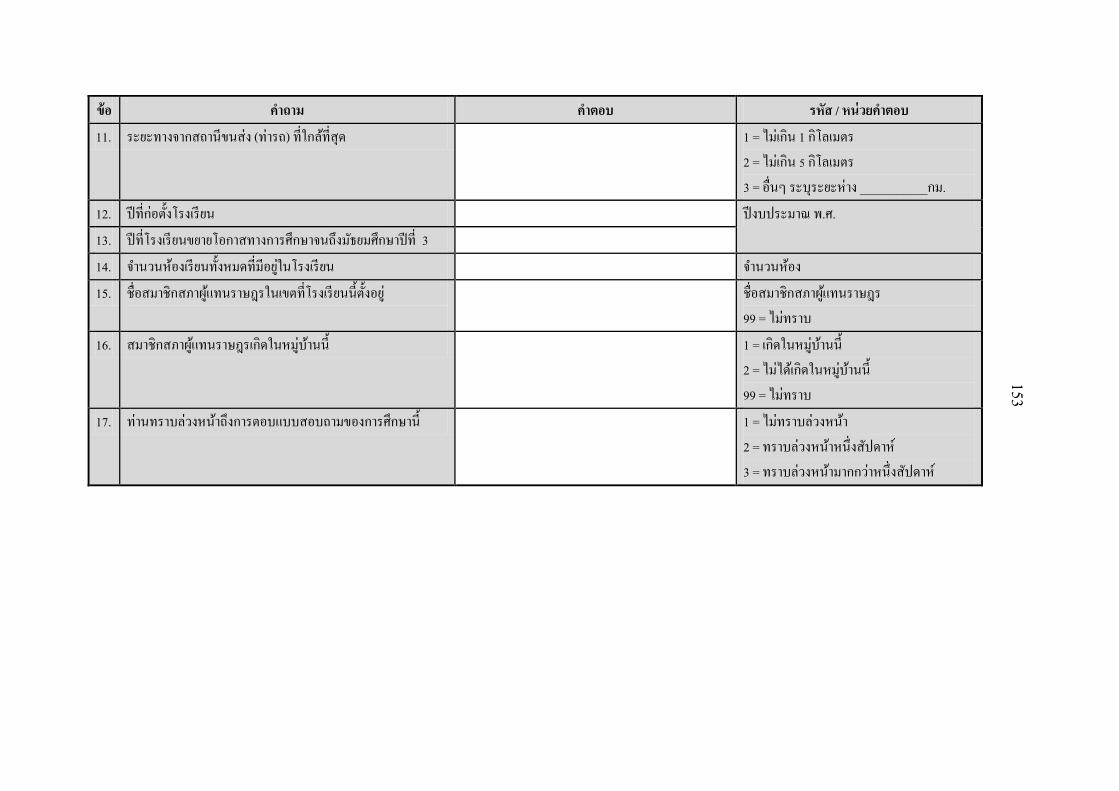
153

ขอ ค าถาม ค าตอบ รหส / หนวยค าตอบ

11. ระยะทางจากสถานขนสง (ทารถ) ทใกลทสด 1 = ไมเกน 1 กโลเมตร 2 = ไมเกน 5 กโลเมตร 3 = อนๆ ระบระยะหาง ___________กม.

12. ปทกอตงโรงเรยน ปงบประมาณ พ.ศ. 13. ปทโรงเรยนขยายโอกาสทางการศกษาจนถงมธยมศกษาปท 3 14. จ านวนหองเรยนทงหมดทมอยในโรงเรยน จ านวนหอง 15. ชอสมาชกสภาผแทนราษฎรในเขตทโรงเรยนนตงอย

ชอสมาชกสภาผแทนราษฎร

99 = ไมทราบ

16. สมาชกสภาผแทนราษฎรเกดในหมบานน 1 = เกดในหมบานน

2 = ไมไดเกดในหมบานน

99 = ไมทราบ 17. ทานทราบลวงหนาถงการตอบแบบสอบถามของการศกษาน 1 = ไมทราบลวงหนา

2 = ทราบลวงหนาหนงสปดาห 3 = ทราบลวงหนามากกวาหนงสปดาห

154

2. ขอมลของผบรหารสถานศกษา (เพอใชเปนตวแปรเชงสถต) ขอ ค าถาม ค าตอบ รหส / หนวยค าตอบ

1. ชอผตอบแบบสอบถาม ชอ 2. เพศ 1 = ชาย

2 = หญง 3. อาย ป 4. สถานภาพ 1 = โสด

2 = สมรส 3 = หยาราง

5. ทานด ารงต าแหนงใดในโรงเรยน 1 = ผบรหารสถานศกษา 2 = รองผบรหารสถานศกษา

6. ทานมภมล าเนาในหมบานน 1 = ม 2 = ไมม 7. ทานมภมล าเนาในอ าเภอน

8. ทานมภมล าเนาในจงหวดน 9. จ านวนปทด ารงต าแหนง ผอ. / รองผอ. ในโรงเรยนน จ านวนป (นบรวมปน) 10. จ านวนปทท างาน (รบราชการคร) กอนทจะด ารงต าแหนง

ผบรหารโรงเรยน (ผอ. / รองผอ.) เปนครงแรก ป

11. จ านวนปทท างาน (รบราชการคร / ผอ. / รอง ผอ.) กอนทจะด ารงต าแหนงผบรหารในโรงเรยนน

ป

155

12. วฒการศกษาของทาน

1 = อนปรญญา

2 = ปรญญาตรดานการศกษา 3 = ปรญญาตรดานอนๆ 4 = ปรญญาโทดานการศกษา 5 = ปรญญาโทดานอนๆ 6 = ปรญญาเอกดานการศกษา 7 = ปรญญาเอกดานอนๆ 88 = อนๆ ระบ

____________________________________ 13. ทานไดรบการฝกอบรม...

(ตอบไดมากกวา 1 ขอ)

1 = ดานการเรยนการสอน 2 = หลกสตรดานการบรหาร 88 = อนๆ ระบ_________________________________

14. ทานไดมาปฏบตงานทโรงเรยนนเพราะ (ตอบไดมากกวา 1 ขอ)

1 = สอบบรรจเขารบราชการในโรงเรยนน 2 = ยายกลบภมล าเนา 3 = เปน ร.ร.ทนาท างานทสด 4 = ไมมต าแหนงวางในโรงเรยนอนๆ 5 = ไมมคนอนๆตองการมาท างานทน 6 = มคนอนๆตองการมาท างานทนแตทาน ไดรบ การพจารณา 88 = อนๆ ระบ ______________________

156

15. หนวยงานทแตงตงใหทานมาด ารงต าแหนงในโรงเรยนน 1 = เลขาธการฯส านกงานงานคณะกรรมการ

การศกษาขนพนฐาน (สพฐ.) 2 = ผอ. ส านกงานเขตพนทการศกษา (สพท.) 3 = อ.ค.ก.ศ. (คณะอนกรรมการขาราชการคร และบคลากรทางการศกษา) 4 = ก.ค.ศ. (คณะกรรมการขาราชการคร และบคลากรทางการศกษา) 5 = คณะกรรมการการประถมศกษาจงหวด (กปจ.) 88 = อนๆ ระบ ____________________

16. บคคล / นตบคคลอนทมสวนใหทานมาด ารงต าแหนงใน โรงเรยนน

1 = ผอ านวยการโรงเรยน 2 = ผน าการเมองทองถน 4 = คณะกรรมการสถานศกษาขนพนฐาน 3 = สมาคมครและผปกครอง 5 = องคกรธรกจทสนบสนนโรงเรยน 6 = องคกรไมแสวงหาก าไร 88 = อนๆ ระบ ____________________

17. ทานมสวนรวมในการตดสนใจเลอกโรงเรยนทมาด ารงต าแหนงมากนอยเพยงไร

0 = ไมมสวนในการตดสนใจเลย 1 = มสวนเลกนอย 2 = มสวนมาก

18. ทานตองการขอยายไปโรงเรยนอนในปตอไปหรอไม 1 = ตองการ 2 = ไมตองการ 99 = ไมทราบ

157

3. ขอมลเกยวกบโรงเรยน (เพอใชเปนตวแปรเชงสถต) ขอ ค าถาม ค าตอบ รหส / หนวยค าตอบ 1. มโรงเรยนอนๆใกลเคยงทนกเรยนจะไปเขาเรยนได 1 = ม 2 = ไมม 99 = ไมทราบ

ถาม โปรดใสชอโรงเรยนใกลเคยงไมเกนสามชอ สงกดโรงเรยน วธการเดนทาง เวลาทใชในการเดนทางจากโรงเรยนนไปยง

โรงเรยนใกลเคยง (เชน 30 นาท, 2 ชวโมง

เปนตน)

1 = สพฐ. 2 = อปท.

1 = เดนไป

2 = ทางรถ 3 = ทางเรอ 88 = อนๆ ระบ________

ก ข ค ง 2. ชอโรงเรยน 3. ชอโรงเรยน 4. ชอโรงเรยน

5. เหตผลหลกทท าใหผปกครองเลอกโรงเรยนน

1 = เปนโรงเรยนยอดนยม 2 = เปนโรงเรยนในเขตพนทบรการ 3 = การเดนทางไป-มาสะดวก 88 = อนๆ ระบ_________________________

ชนดของหองเรยน จ านวนหองเรยน จ านวนหองเรยนทเกาหรอเสยหายท จะตองซอมแซมบางสวน

จ านวนหองเรยนทเกาหรอเสยหายท จะตองสรางใหม

ก ข ค 6. หองเรยนถาวร

7. หองเรยนกงถาวร

158

8. หองเรยนชวคราว

9. จ านวนหองเรยนทงหมดทมกระดานส าหรบสอนหนาหองเรยน โปรดใสจ านวนหองเรยน 10. จ านวนหองเรยนทงหมดทมไฟฟาใช 11. จ านวนหองเรยนทงหมดทมโตะและเกาอส าหรบครผสอน 12. จ านวนหองเรยนทงหมดทมชองเกบของทสามารถลอคได

เพอเกบอปกรณการเรยนการสอนในตอนกลางคน

13. จ านวนหองเรยนทงหมดทมหลงคารวเวลาฝนตก

ประเภทของบานพกคร จ านวนทใชท าเปนบานพกคร จ านวนบานทเกาหรอเสยหาย ทจะตองซอมแซมบางสวน

จ านวนบานทเกาหรอ เสยหายทจะตอง

สรางใหม ก ข ค

14. บานพกถาวร

15. บานพกชวคราว (เชน พกอาศยในอาคารอนของโรงเรยน)

16. อนๆ ระบ __________________________________________

โรงเรยนมสงเหลานหรอไม 17. หองสมด 0 = ไมม

1 = มจ านวนหนงแตไมเพยงพอ 2 = มจ านวนเพยงพอใชงานได 3 = มจ านวนมากเพยงพอใหใชงาน

18. หองพกคร 19. หองของฝายธรการหรอเจาหนาทฝายบรหารตางๆ 20. ยานพาหนะของโรงเรยน 21. บรเวณทท าการเพาะปลกพชผกส าหรบนกเรยน 22. บรเวณทท าการเพาะปลกพชผกส าหรบคร

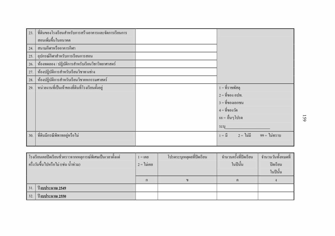
159

23. ทดนของโรงเรยนส าหรบการสรางอาคารและจดการเรยนการ

สอนเพมขนในอนาคต

24. สนามกฬาหรออาคารกฬา 25. อปกรณกฬาส าหรบการเรยนการสอน 26. หองทดลอง / ปฏบตการส าหรบเรยนวชาวทยาศาสตร 27. หองปฏบตการส าหรบเรยนวชาทางชาง 28. หองปฏบตการส าหรบเรยนวชาคหกรรมศาสตร 29. หนวยงานทเปนเจาของทดนทโรงเรยนตงอย 1 = ทราชพสด

2 = ทของ อปท. 3 = ทของเอกชน 4 = ทของวด 88 = อนๆโปรด

ระบ________________

30. ทดนมกรณพพาทอยหรอไม 1 = ม 2 = ไมม 99 = ไมทราบ

โรงเรยนเคยปดเรยนชวคราวจากเหตการณพเศษเปนเวลาตงแต ครงวนขนไปหรอไม (เชน น าทวม)

1 = เคย 2 = ไมเคย

โปรดระบเหตผลทปดเรยน จ านวนครงทปดเรยน ในปนน

จ านวนวนทงหมดทปดเรยน ในปนน

ก ข ค ง 31. ปงบประมาณ 2549

32. ปงบประมาณ 2550

160

33. โรงเรยนนมไฟฟาใช 1 = มใช 2 = ไมมใช

34. โรงเรยนนมถงน าส าหรบเกบน าไวใช 1 = มใช 2 = ไมมใช

35. แหลงน าหลกส าหรบใชดมในโรงเรยนน 0 = ไมมแหลงน าหลก 1 = ถงเกบน าฝน 2 = สระน า / อางน า / แมน า 3 = บอน าบาดาล 4 = ทอน าประปา 88 = อนๆ ระบ __________________________

36. ปจจบนนกเรยนยงสามารถใชน าดมจากแหลงน าในขอ 35 ส าหรบดมได

1 = ใชได 2 = ใชไมได 99 = ไมทราบ

37. มน าใชเพยงพอจากแหลงนตลอดปงบประมาณ 2550 1 = มเพยงพอ 2 = ไมเพยงพอ 99 = ไมทราบ

38. ประเภทของหองสขาส าหรบครในโรงเรยนน 1 = แบบคอหาน 2 = แบบโถนง

39. ถาเปนแบบโถนง : มน าเพยงพอใชไดตลอดเวลา (ถาเปนแบบคอหานโปรดท าเครองหมาย — ในชองค าตอบ)

1 = ไมมน าใชเลย 2 = มน าใชแตไมสม าเสมอ 3 = มน าเพยงพอใชไดตลอดเวลา

40. ประเภทของหองสขาส าหรบนกเรยนชายในโรงเรยนน 1 = ไมม 2 = แบบคอหาน 3 = แบบโถนง

41. ถาเปนแบบโถนง : มน าเพยงพอใชไดตลอดเวลา 1 = ไมมน าใชเลย

161

(ถาเปนแบบคอหานโปรดท าเครองหมาย — ในชองค าตอบ) 2 = มน าใชแตไมสม าเสมอ

3 = มน าเพยงพอใชไดตลอดเวลา

42. มหองสขาเพยงพอส าหรบนกเรยนชาย

1 = มเพยงพอ 2 = ไมเพยงพอ 99 = ไมทราบ

43. ถาไมเพยงพอ : โรงเรยนตองการหองสขาเพมอกจ านวนกหอง (ถาไมตองการโปรดท าเครองหมาย — ในชองค าตอบ)

1 = 1-3 หอง 2 = 4-6 หอง 3 = 7-10 หอง 4 = มากกวา 10 หอง

44. ประเภทของหองสขาส าหรบนกเรยนหญงในโรงเรยนน 1 = แบบคอหาน 2 = แบบโถนง

45. ถาเปนแบบโถนง : มน าเพยงพอใชไดตลอดเวลา (ถาเปนแบบคอหานโปรดท าเครองหมาย — ในชองค าตอบ)

1 = ไมมน าใชเลย 2 = มน าใชแตไมสม าเสมอ 3 = มน าเพยงพอใชไดตลอดเวลา

46. มหองสขาเพยงพอส าหรบนกเรยนหญง

1 = มเพยงพอ 2 = ไมเพยงพอ 99 = ไมทราบ

47. ถาไมเพยงพอ : โรงเรยนตองการหองสขาเพมอกจ านวนกหอง (ถาไมตองการโปรดท าเครองหมาย — ในชองค าตอบ)

1 = 1-3 หอง 2 = 4-6 หอง 3 = 7-10 หอง 4 = มากกวา 10 หอง

ระยะทางใกลทสดของสถานทเหลานกบโรงเรยน

162

ระยะทาง (กม.) เดนทางโดย เวลาทใชในการเดนทางจากโรงเรยนนไปยง

สถานทเหลาน (เชน 30 นาท, 2 ชวโมง เปนตน)

0 = อยในโรงเรยน 1 = ภายใน 1 กม. 2 = ภายใน 5 กม. 3 = ภายใน 20 กม. 4 = มากกวา 20 กม. 99 = ไมทราบ

1 = เดนไป

2 = ทางรถ 3 = ทางเรอ

ก ข ค

48. โรงเรยนมธยมศกษาอนๆ 49. สถานบรการสาธารณสข 50. สถานฝกอาชพ 51. รานขายเครองเขยน (สมด, ดนสอ) 52. รานขายของช าทวไป 53. สถานท าการไปรษณย 54. ธนาคาร 55. สถานต ารวจ 56. ถนนราดยางมะตอยหรอคอนกรต 57. บรเวณทจอดรถโดยสาร (ปายรถ) 58. สถานขนสง 59. ทท าการเทศบาล / อบต. / อบจ. 60. โทรศพทสาธารณะทใชการได 61. ทาเรอทมเรอบรการเปนประจ า

163

ปงบประมาณ 2549 ปงบประมาณ 2550 รหส / หนวยค าตอบ

62. โรงเรยนมรวลอมรอบปองกนผบกรกในปงบประมาณ… 1 = มรว 2 = ไมมรว 3 = มรวแตไมครบทกดาน 99 = ไมทราบ

63. บานพกครมรวลอมรอบปองกนผบกรกในปงบประมาณ… 1 = มรว 2 = ไมมรว 3 = มรวแตไมครบทกดาน 4 = ไมมบานพกคร 99 = ไมทราบ

64. ทานไดจางเจาหนาทรกษาความปลอดภยในปงบประมาณ… 1 = จาง 2 = ไมจาง 99 = ไมทราบ

65. จ านวนงบประมาณทงหมดทใชในเรองการรกษา

ความปลอดภยตอป

บาท

66. จ านวนครงทโรงเรยนถกบกรกในปงบประมาณ… จ านวนครงทถกบกรก 0 = ไมเคยถกบกรก

67. มลคาความเสยหายจากการถกขโมยหรอถกท าลายใน

ปงบประมาณ…

บาท

164

4. ขอมลเกยวกบการตรวจเยยมโรงเรยน (เพอใชเปนตวแปรเชงสถต) ขอ ค าถาม ค าตอบ รหส / หนวยค าตอบ

ปการศกษา 2549 ปการศกษา 2550 1. จ านวนครงทมผตรวจเยยมโรงเรยนในปงบประมาณ…

จ านวนครง

2. วตถประสงคของการตรวจเยยมในครงลาสด 1 = ตรวจเยยมเปนการสวนตว 2 = ตรวจเยยมตามค าสงพเศษ 3 = ตรวจเยยมตามก าหนดการปกต 88 = อนๆ โปรดระบ ______________________________

ในขณะตรวจเยยม ผตรวจเยยมได…. 3. …พบกบผบรหารสถานศกษา 1 = ใช

2 = ไมใช 99 = ไมทราบ

4. …พบกบคร 5. …พบกบคณะกรรมการสถานศกษาขนพนฐาน 6. …พบกบผปกครอง 7. …เขาสงเกตการเรยนการสอน 8. …ตรวจสอบรายงานตางๆของโรงเรยน

165

9. ภายหลงการตรวจเยยม วธการรายงาน

การตรวจเยยม…. (ตอบไมเกน 3 ค าตอบ)

10ก 0 = ไมมการรายงาน 1 = ดวยวาจาในการประชมคร 2 = ดวยวาจากบผอ านวยการ 3 = ดวยวาจากบครแตละคน 4 = ดวยลายลกษณอกษรกบผอ านวยการ 5 = ดวยลายลกษณอกษรกบครแตละคน

10ข

10ค

ขอ ค าถาม ค าตอบ รหส / หนวยค าตอบ ปงบประมาณ 2549 ปงบประมาณ 2550 10. โรงเรยนไดรบผลการตรวจเยยมเปนลายลกษณอกษรใน

ภายหลง 1 = ไดรบ

2 = ไมไดรบ 11. ถาไดรบ : เวลาทไดรบรายงานภายหลงการตรวจเยยม

โรงเรยน (ถาไมไดรบโปรดท าเครองหมาย — ในชองค าตอบ)

จ านวนวน

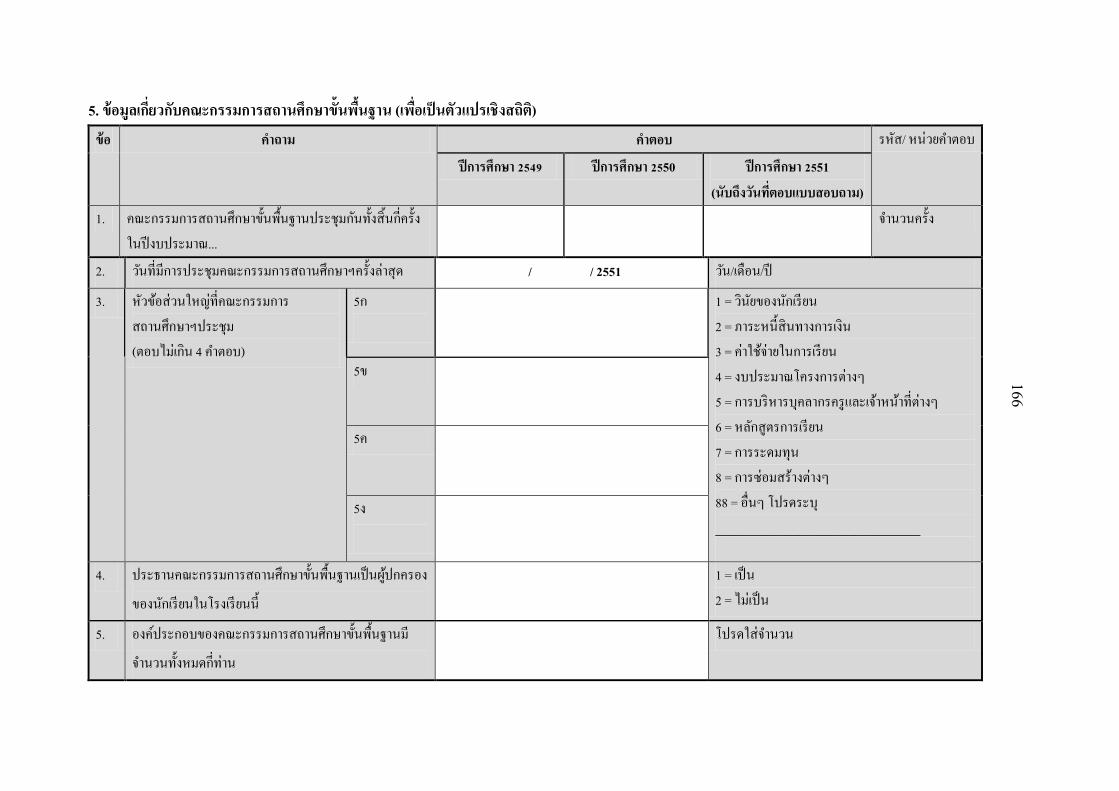
166

5. ขอมลเกยวกบคณะกรรมการสถานศกษาขนพนฐาน (เพอเปนตวแปรเชงสถต) ขอ ค าถาม ค าตอบ รหส/ หนวยค าตอบ

ปการศกษา 2549 ปการศกษา 2550 ปการศกษา 2551 (นบถงวนทตอบแบบสอบถาม)

1. คณะกรรมการสถานศกษาขนพนฐานประชมกนทงสนกครง ในปงบประมาณ...

จ านวนครง

2. วนทมการประชมคณะกรรมการสถานศกษาฯครงลาสด / / 2551 วน/เดอน/ป

3. หวขอสวนใหญทคณะกรรมการ สถานศกษาฯประชม (ตอบไมเกน 4 ค าตอบ)

5ก

1 = วนยของนกเรยน 2 = ภาระหนสนทางการเงน 3 = คาใชจายในการเรยน 4 = งบประมาณโครงการตางๆ 5 = การบรหารบคลากรครและเจาหนาทตางๆ 6 = หลกสตรการเรยน 7 = การระดมทน 8 = การซอมสรางตางๆ 88 = อนๆ โปรดระบ ______________________

5ข

5ค

5ง

4. ประธานคณะกรรมการสถานศกษาขนพนฐานเปนผปกครอง

ของนกเรยนในโรงเรยนน

1 = เปน 2 = ไมเปน

5. องคประกอบของคณะกรรมการสถานศกษาขนพนฐานม

จ านวนทงหมดกทาน

โปรดใสจ านวน

167

6. ทมาของตวแทนของคณะกรรมการสถานศกษาขนพนฐาน โปรดใสจ านวนของตวแทน

ตวแทนชาย ตวแทนหญง

6ก. จากผบรหารโรงเรยน

6ข. จากครและบคลากรในโรงเรยน

6ค. จากผปกครอง

6ง. จากองคกรปกครองสวนทองถน

6จ. จากผทรงคณวฒ

6ฉ. จากศษยเกา

6ช. จากองคกรศาสนา

6ซ. จากองคกรชมชน ระบ

_______________________________

6ฌ. อนๆ ระบ

_______________________________

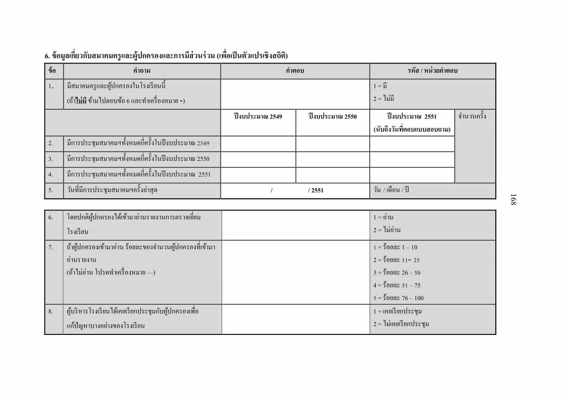
168

6. ขอมลเกยวกบสมาคมครและผปกครองและการมสวนรวม (เพอเปนตวแปรเชงสถต) ขอ ค าถาม ค าตอบ รหส / หนวยค าตอบ

1. มสมาคมครและผปกครองในโรงเรยนน

(ถาไมม ขามไปตอบขอ 6 และท าเครองหมาย -)

1 = ม 2 = ไมม

ปงบประมาณ 2549 ปงบประมาณ 2550 ปงบประมาณ 2551 (นบถงวนทตอบแบบสอบถาม)

จ านวนครง

2. มการประชมสมาคมฯทงหมดกครงในปงบประมาณ 2549

3. มการประชมสมาคมฯทงหมดกครงในปงบประมาณ 2550

4. มการประชมสมาคมฯทงหมดกครงในปงบประมาณ 2551

5. วนทมการประชมสมาคมฯครงลาสด / / 2551 วน / เดอน / ป

6. โดยปกตผปกครองไดเขามาอานรายงานการตรวจเยยม

โรงเรยน

1 = อาน 2 = ไมอาน

7. ถาผปกครองเขามาอาน รอยละของจ านวนผปกครองทเขามาอานรายงาน (ถาไมอาน โปรดท าเครองหมาย —)

1 = รอยละ 1 – 10 2 = รอยละ 11- 25 3 = รอยละ 26 – 50 4 = รอยละ 51 – 75 5 = รอยละ 76 – 100

8. ผบรหารโรงเรยนไดเคยเรยกประชมกบผปกครองเพอ

แกปญหาบางอยางของโรงเรยน

1 = เคยเรยกประชม 2 = ไมเคยเรยกประชม

169

9. ถาเคยเรยก : จ านวนรอยละของผทเขารวมประชม

(ถาไมอาน โปรดท าเครองหมาย —) 1 = รอยละ 1 – 10

2 = รอยละ 11- 25 3 = รอยละ 26 – 50 4 = รอยละ 51 – 75 5 = รอยละ 76 – 100

10. ครไดเคยมการจดกจกรรมรวมกบชมชนเกยวกบการศกษา /การอบรม

1 = เคย 2 = ไมเคย 99 = ไมทราบ 11. สมาชกในชมชนไดเคยเขามารวมท ากจกรรมทาง

ศลปวฒนธรรม

12. ชมชนใหโรงเรยนใชทดนในการเรยนการสอน

วชาเกษตรกรรม

1 = ใหใช 2 = ไมใหใช 3 = ไมมการสอนวชาน 99 = ไมทราบ

13. ชมชนไดเคยใชสถานทของโรงเรยน…. 1 = ใช 2 = ไมใช 99 = ไมทราบ

13ก. …ใชในการจดการประชม

13ข. …ใชในการศกษาอบรมของชมชน

13ค. …ใชในการจดกฬาของชมชน

170

7. ขอมลเกยวกบการเงนของโรงเรยนและแหลงเงนสนบสนน (เพอเปนตวแปรเชงสถต)

1. จ านวนเงนคาเทอมทไดรบจากผปกครองนกเรยน (ตอ 1 คนตอ 1 ป) รหส / หนวยค าตอบ

ก. ชนอนบาล ข. ชนประถมศกษา ค. ชนมธยมศกษาตอนตน 2549 จ านวนเงน (บาท)

0 = โรงเรยนไมเรยกเกบ

(โปรดท าเครองหมาย – ในชองทไมมขอมล) 2550

2551

2. จ านวนเงนคาใชจายอนๆ ทไดรบจากผปกครองนกเรยน เชน ชดกฬา, การไปทศนศกษานอกสถานท เปนตน (ตอ 1 คนตอ 1 ป) รหส / หนวยค าตอบ ก. ชนอนบาล ข. ชนประถมศกษา ค. ชนมธยมศกษาตอนตน

2549 จ านวนเงน (บาท) 0 = โรงเรยนไมเรยกเกบ (โปรดท าเครองหมาย – ในชองทไมมขอมล)

2550

2551

ขอ ค าถาม ค าตอบ รหส / หนวยค าตอบ

3. ค าตอบในขอ 1. และ ขอ 2. มาจากแหลงขอมลใด 1 = จากบนทกของโรงเรยน 2 = จากบนทกของคณะกรรมการสถานศกษา ขนพนฐาน ของโรงเรยน 3 = จากความทรงจ าผตอบ

171

ค าถาม ปงบประมาณ

2549 ปงบประมาณ

2550 ปงบประมาณ

2551 รหส / หนวยค าตอบ

4. วธการช าระคาเทอมของผปกครองนกเรยนในปงบประมาณ (ตอบไดมากกวา 1 ขอและถาไมมคาเทอมขามไปท าขอ 10)

1 = ช าระตอนเปดภาคเรยนทงหมด 2 = ช าระบางสวนตอนตนเทอมและทเหลอ ช าระ เปนรายเดอนจนครบ 3 = แบงช าระเปนรายเดอนเทาๆกนจนครบ

4 = โรงเรยนรบภาระในสวนทผปกครองจาย ไมได 5 = อนๆระบ _______________________

5. จ านวนผปกครองทสามารถช าระคาเทอม ทงหมดได

จ านวนรอยละ (เชน รอยละ 90 ของผปกครองจายคาเทอมได)

6. ถาผปกครองไมสามารถจายคาเทอมได มมาตรการใดในการชวยเหลอนกเรยน

โปรดเขยนมาตรการ

7. จ านวนนกเรยนทโรงเรยนรบภาระในสวนทผปกครองจายคาเทอมไมได

จ านวนนกเรยนโดยประมาณ (คน)

8. จ านวนเงนคาเทอมทผปกครองยงคางช าระใหแกโรงเรยนเมอสนปงบประมาณ...

บาท

172

ปงบประมาณ

2549 ปงบประมาณ

2550 ปงบประมาณ

2551 รหส / หนวยค าตอบ

9. วธการช าระคาใชจายอนๆของผปกครองนกเรยนในปงบประมาณ…

(ตอบไดมากกวา 1 ขอและถาไมมคาใชจายอนขามไปท า ขอ 15)

1 = ช าระตอนเปดภาคเรยนทงหมด 2 = ช าระบางสวนตอนตนเทอมและทเหลอ ช าระ เปนรายเดอนจนครบ 3 = แบงช าระเปนรายเดอนเทาๆกนจนครบ 4 = โรงเรยนรบภาระในสวนทผปกครองจาย ไมได 5 = อนๆระบ _____________________________

10. จ านวนผปกครองทสามารถช าระคาใชจายอนๆได จ านวนรอยละ (เชน รอยละ 90 สามารถช าระคาใชจายอนได)

11. ถาผปกครองไมสามารถจายคาใชจายอนๆได มมาตรการใดในการชวยเหลอนกเรยน

โปรดเขยนมาตรการ

12. จ านวนนกเรยนทโรงเรยนรบภาระในสวนทผปกครองจาย คาใชจายอนๆไมได

จ านวนนกเรยนโดยประมาณ (คน)

13. จ านวนเงนคาใชจายอนๆทผปกครองยงคางช าระใหแกโรงเรยนเมอสนปงบประมาณ...

บาท

173

14. จ านวนเงนทรฐอดหนนนกเรยนในโรงเรยนน

ตอหวในปงบประมาณ….. ปงบประมาณ

2549 ปงบประมาณ

2550 ปงบประมาณ

2551 รหส / หนวยค าตอบ

14ก. ชนอนบาล บาท 14ข. ชนประถมศกษา 14ค. ชนมธยมศกษาศกษาตอนตน

การสนบสนนการศกษาในปงบประมาณ 2549 (เพอเปนตวแปรเชงสถต) ภาคเรยนท 2/2548 ภาคเรยนท 1/2549 รหส / หนวยค าตอบ 15. โรงเรยนไดรบเงนสนบสนนในรป…

1 = เงนสด

2 = โอนเขาธนาคาร 3 = เชค

16. โรงเรยนไดรบงบประเภทเงนรายหวจ านวนทงสนเทาใด บาท

17. โรงเรยนไดรบงบประเภทเงนรายหวในเดอนใด 1 = ม.ค. 2 = ก.พ. 3 = ม.ค. 4 = เม.ย. 5 = พ.ค. 6 = ม.ย. 7 = ก.ค. 8 = ส.ค. 9 = ก.ย. 10 = ต.ค. 11 = พ.ย. 12 = ธ.ค.

18. โดยปกตเวลาทใชในขนตอนการเบกจายกอนทจะสามารถน า งบประเภทเงนรายหวไปใชได

เวลา (วน)

19. โรงเรยนไดรบงบประเภทเงนอดหนนทงสนเทาใด บาท

20. โรงเรยนไดรบงบประเภทเงนอดหนนในเดอนใด

1 = ม.ค. 2 = ก.พ. 3 = ม.ค. 4 = เม.ย. 5 = พ.ค. 6 = ม.ย. 7 = ก.ค. 8 = ส.ค. 9 = ก.ย. 10 = ต.ค. 11 = พ.ย. 12 = ธ.ค.

21. โดยปกตเวลาทใชในขนตอนการเบกจายกอนทจะน า งบประเภทเงนอดหนนไปใชได

เวลา (วน)

174

ภาคเรยนท 2/2548 ภาคเรยนท 1/2549 รหส / หนวยค าตอบ

22. โรงเรยนไดรบงบประเภทรายจายอนทงสนเทาใด บาท

23. โรงเรยนไดรบงบประเภทรายจายอนในเดอนใด 1 = ม.ค. 2 = ก.พ. 3 = ม.ค. 4 = เม.ย.

5 = พ.ค. 6 = ม.ย. 7 = ก.ค. 8 = ส.ค. 9 = ก.ย. 10 = ต.ค. 11 = พ.ย. 12 = ธ.ค.

24. โดยปกตเวลาทใชในขนตอนการเบกจายกอนทจะน า งบประเภทรายจายอนไปใชได

จ านวนวน

25. โรงเรยนไดรบการสนบสนนในรปสงของอนๆหรอไม (เชน หนงสอเรอน, อปกรณการเรยนการสอน)

1 = ไดรบ 2 = ไมไดรบ

26. โรงเรยนไดรบหนงสอเรยนเปนมลคาทงสนเทาใด บาท 27. โรงเรยนไดรบหนงสอเรยนในเดอนใด 1 = ม.ค. 2 = ก.พ. 3 = ม.ค. 4 = เม.ย.

5 = พ.ค. 6 = ม.ย. 7 = ก.ค. 8 = ส.ค. 9 = ก.ย. 10 = ต.ค. 11 = พ.ย. 12 = ธ.ค.

28. โรงเรยนไดรบอปกรณการเรยนการสอนเปนมลคาทงสน เทาใด

บาท

29. โรงเรยนไดรบอปกรณการเรยนการสอนในเดอนใด 1 = ม.ค. 2 = ก.พ. 3 = ม.ค. 4 = เม.ย. 5 = พ.ค. 6 = ม.ย. 7 = ก.ค. 8 = ส.ค. 9 = ก.ย. 10 = ต.ค. 11 = พ.ย. 12 = ธ.ค.

30. บรษท/หนวยงานทผลตสงของน (เชน หนงสอเรอน, อปกรณการเรยนการสอน)

ชอบรษท/หนวยงาน 0 = ไมทราบชอผผลต

175

การสนบสนนการศกษาในปงบประมาณ 2550 (เพอเปนตวแปรเชงสถต) ภาคเรยนท 2/2549 ภาคเรยนท 1/2550 รหส / หนวยค าตอบ

31. โรงเรยนไดรบเงนสนบสนนในรป…

1 = เงนสด 2 = โอนเขาธนาคาร 3 = เชค

32. โรงเรยนไดรบงบประเภทเงนรายหวจ านวนทงสนเทาใด บาท

33. โรงเรยนไดรบงบประเภทเงนรายหวในเดอนใด 1 = ม.ค. 2 = ก.พ. 3 = ม.ค. 4 = เม.ย. 5 = พ.ค. 6 = ม.ย. 7 = ก.ค. 8 = ส.ค. 9 = ก.ย. 10 = ต.ค. 11 = พ.ย. 12 = ธ.ค.

34. โดยปกตเวลาทใชในขนตอนการเบกจายกอนทจะสามารถน า งบประเภทเงนรายหวไปใชได

เวลา (วน)

35. โรงเรยนไดรบงบประเภทเงนอดหนนทงสนเทาใด บาท

36. โรงเรยนไดรบงบประเภทเงนอดหนนในเดอนใด

1 = ม.ค. 2 = ก.พ. 3 = ม.ค. 4 = เม.ย. 5 = พ.ค. 6 = ม.ย. 7 = ก.ค. 8 = ส.ค. 9 = ก.ย. 10 = ต.ค. 11 = พ.ย. 12 = ธ.ค.

37. โดยปกตเวลาทใชในขนตอนการเบกจายกอนทจะน า งบประเภทเงนอดหนนไปใชได

เวลา (วน)

38. โรงเรยนไดรบงบประเภทรายจายอนทงสนเทาใด บาท

39. โรงเรยนไดรบงบประเภทรายจายอนในเดอนใด 1 = ม.ค. 2 = ก.พ. 3 = ม.ค. 4 = เม.ย. 5 = พ.ค. 6 = ม.ย. 7 = ก.ค. 8 = ส.ค. 9 = ก.ย. 10 = ต.ค. 11 = พ.ย. 12 = ธ.ค.

176

ภาคเรยนท 2/2549 ภาคเรยนท 1/2550 รหส / หนวยค าตอบ

40. โดยปกตเวลาทใชในขนตอนการเบกจายกอนทจะน า งบประเภทรายจายอนไปใชได

จ านวนวน

41. โรงเรยนไดรบการสนบสนนในรปสงของอนๆหรอไม (เชน หนงสอเรอน, อปกรณการเรยนการสอนอน)

1 = ไดรบ 2 = ไมไดรบ

42. โรงเรยนไดรบหนงสอเรยนเปนมลคาทงสนเทาใด บาท

43. โรงเรยนไดรบหนงสอเรยนในเดอนใด 1 = ม.ค. 2 = ก.พ. 3 = ม.ค. 4 = เม.ย. 5 = พ.ค. 6 = ม.ย. 7 = ก.ค. 8 = ส.ค. 9 = ก.ย. 10 = ต.ค. 11 = พ.ย. 12 = ธ.ค.

44. โรงเรยนไดรบอปกรณการเรยนการสอนเปนมลคาทงสน เทาใด

บาท

45. โรงเรยนไดรบอปกรณการเรยนการสอนในเดอนใด 1 = ม.ค. 2 = ก.พ. 3 = ม.ค. 4 = เม.ย. 5 = พ.ค. 6 = ม.ย. 7 = ก.ค. 8 = ส.ค. 9 = ก.ย. 10 = ต.ค. 11 = พ.ย. 12 = ธ.ค.

46. บรษท/หนวยงานทผลตสงของน

ชอบรษท/หนวยงาน 0 = ไมทราบชอผผลต

177

การสนบสนนการศกษาในปงบประมาณ 2551 (เพอเปนตวแปรเชงสถต) รหส / หนวยค าตอบ

ภาคเรยนท 2/2550

47. โรงเรยนไดรบเงนสนบสนนในรป…

1 = เงนสด 2 = โอนเขาธนาคาร 3 = เชค

48. โรงเรยนไดรบงบประเภทเงนรายหวจ านวนทงสนเทาใด บาท 49. โรงเรยนไดรบงบประเภทเงนรายหวในเดอนใด 1 = ม.ค. 2 = ก.พ. 3 = ม.ค. 4 = เม.ย.

5 = พ.ค. 6 = ม.ย. 7 = ก.ค. 8 = ส.ค. 9 = ก.ย. 10 = ต.ค. 11 = พ.ย. 12 = ธ.ค.

50. โดยปกตเวลาทใชในขนตอนการเบกจายกอนทจะสามารถน า งบประเภทเงนรายหวไปใชได

เวลา (วน)

51. โรงเรยนไดรบงบประเภทเงนอดหนนทงสนเทาใด บาท 52. โรงเรยนไดรบงบประเภทเงนอดหนนในเดอนใด

1 = ม.ค. 2 = ก.พ. 3 = ม.ค. 4 = เม.ย.

5 = พ.ค. 6 = ม.ย. 7 = ก.ค. 8 = ส.ค. 9 = ก.ย. 10 = ต.ค. 11 = พ.ย. 12 = ธ.ค.

53. โดยปกตเวลาทใชในขนตอนการเบกจายกอนทจะน า งบประเภทเงนอดหนนไปใชได

เวลา (วน)

54. โรงเรยนไดรบงบประเภทรายจายอนทงสนเทาใด บาท

55. โรงเรยนไดรบงบประเภทรายจายอนในเดอนใด 1 = ม.ค. 2 = ก.พ. 3 = ม.ค. 4 = เม.ย. 5 = พ.ค. 6 = ม.ย. 7 = ก.ค. 8 = ส.ค. 9 = ก.ย. 10 = ต.ค. 11 = พ.ย. 12 = ธ.ค.

178

56. โดยปกตเวลาทใชในขนตอนการเบกจายกอนทจะน า

งบประเภทรายจายอนไปใชได จ านวนวน

57. โรงเรยนไดรบการสนบสนนในรปสงของอนๆหรอไม (เชน หนงสอเรอน, อปกรณการเรยนการสอนอน)

1 = ไดรบ 2 = ไมไดรบ

58. โรงเรยนไดรบหนงสอเรยนเปนมลคาทงสนเทาใด บาท

59. โรงเรยนไดรบหนงสอเรยนในเดอนใด 1 = ม.ค. 2 = ก.พ. 3 = ม.ค. 4 = เม.ย. 5 = พ.ค. 6 = ม.ย. 7 = ก.ค. 8 = ส.ค. 9 = ก.ย. 10 = ต.ค. 11 = พ.ย. 12 = ธ.ค.

60. โรงเรยนไดรบอปกรณการเรยนการสอนเปนมลคาทงสน เทาใด

บาท

61. โรงเรยนไดรบอปกรณการเรยนการสอนในเดอนใด 1 = ม.ค. 2 = ก.พ. 3 = ม.ค. 4 = เม.ย. 5 = พ.ค. 6 = ม.ย. 7 = ก.ค. 8 = ส.ค. 9 = ก.ย. 10 = ต.ค. 11 = พ.ย. 12 = ธ.ค.

62. บรษท/หนวยงานทผลตสงของน

ชอบรษท/หนวยงาน 0 = ไมทราบชอผผลต

179

63. นอกจากงบประมาณของรฐแลว โรงเรยนไดเงนสนบสนนจากแหลงใดบาง ปงบประมาณ 2549 ปงบประมาณ 2550 รหส / หนวยค าตอบ 63ก. องคกรปกครองสวนทองถน

ระบ __________________________________________

บาท

63ข. วด/โบสถ ระบ ____________________________

63ค. องคกรไมแสวงหาก าไร ระบ __________________________________________

63ง. ผน าการเมองทองถน ระบ __________________________________________

63จ. องคกรจากตางประเทศ ระบ __________________________________________

63ฉ. องคกรเอกชน ระบ __________________________________________

63ช. การจดกจกรรมระดมทนของโรงเรยน ระบ __________________________________________

180

64. นอกจากงบประมาณของรฐแลว โรงเรยนไดมลคาสงของสนบสนนทไมเปนตวเงนจากแหลงใดอกบาง ปงบประมาณ 2549 ปงบประมาณ 2550 รหส / หนวยค าตอบ 64ก. องคกรปกครองสวนทองถน

ระบ __________________________________________

บาท

64ข. วด/โบสถ ระบ __________________________________________

64ค. องคกรไมแสวงหาก าไร ระบ __________________________________________

64ง. ผน าการเมองทองถน ระบ __________________________________________

64จ. องคกรจากตางประเทศ ระบ __________________________________________

64ฉ. องคกรเอกชนตางๆ ระบ __________________________________________

64ช. การจดกจกรรมระดมทนของโรงเรยน ระบ __________________________________________

181

ปงบประมาณ

2549 ปงบประมาณ

2550 ปงบประมาณ

2551

65. จ านวนหองเรยนทเรมตนสรางในโรงเรยนนตงแตปงบ….

จ านวน

0 = ไมมการสราง

66. จ านวนบานพกครทเรมตนสรางในโรงเรยนนตงแตปงบ….

67. จ านวนสงกอสรางอนๆ (เชน หองท างานฝายบรหาร, หองสมด) ทเรมตนสรางในโรงเรยนนตงแตปงบ….

68. จ านวนทสรางเสรจทงหมดในปงบ.....

69. จ านวนบญชธนาคารทงหมดของโรงเรยนในปจจบน จ านวน

70. โปรดระบประเภทบญช

มบญชธนาคารหลกรวมกนของโรงเรยนและคณะกรรมการสถานศกษาขนพนฐาน

1 = ม

2 = ไมม

(โปรดตอบแบบสอบถามในสวนทโรงเรยน มบญชธนาคารดงกลาวทกบญช)

71. มบญชธนาคารหลกของโรงเรยน

72. มบญชธนาคารหลกของคณะกรรมการสถานศกษาขนพนฐาน

73. มบญชธนาคารอนๆเพองานของโรงเรยน

ระบ ___________________

___________________

182

กรณมการใชบญชธนาคารหลกรวมกนของโรงเรยนและคณะกรรมการสถานศกษาขนพนฐาน (เพอทราบแนวทางการบรหารงบประมาณ)

ขอ ค าถาม ค าตอบ หนวย

74. จ านวนเงนทงหมดทเบกออกจากบญชธนาคารหลกรวมกนของโรงเรยนและคณะกรรมการสถานศกษาขนพนฐาน เพองานดงตอไปนในปงบประมาณ….

บญชหลก บาท

ปงบประมาณ 2549 ปงบประมาณ 2550

74ก. การซอมแซมทวๆไป

74ข. การสรางอาคารสถานทตางๆ

74ค. ครภณฑพนฐานตางๆ

74ง. หนงสอและต าราเรยน

74จ. วสดสนเปลองตางๆ

74ฉ. อปกรณการเรยนการสอน

74ช. การเดนทางและการขนสง

74ซ. จางคนท างานพเศษ

74ฌ. ครจางสอน

74ญ. อนๆ ระบ _________________________________

______________________

183

กรณมบญชธนาคารหลกของโรงเรยน (เพอทราบแนวทางการบรหารงบประมาณ)

ขอ ค าถาม ค าตอบ หนวย

75. จ านวนเงนทงหมดทเบกออกจากบญชธนาคารหลกของโรงเรยน เพองานดงตอไปนในปงบประมาณ….

บญชหลก บาท

ปงบประมาณ 2549 ปงบประมาณ 2550

75ก. การซอมแซมทวๆไป

75ข. การสรางอาคารสถานทตางๆ

75ค. ครภณฑพนฐานตางๆ

75ง. หนงสอและต าราเรยน

75จ. วสดสนเปลองตางๆ

75ฉ. อปกรณการเรยนการสอน

75ช. การเดนทางและการขนสง

75ซ. จางคนท างานพเศษ

75ฌ. ครจางสอน

75ญ. อนๆ ระบ ________________________________

_____________________

184

กรณม บญชธนาคารหลก ของคณะกรรมการสถานศกษาขนพนฐาน (เพอทราบแนวทางการบรหารงบประมาณ)

ขอ ค าถาม ค าตอบ หนวย

76. จ านวนเงนทงหมดทเบกออกจากบญชธนาคารหลกของคณะกรรมการสถานศกษาขนพนฐาน เพองานดงตอไปนในปงบประมาณ….

บญชหลก บาท

ปงบประมาณ 2549 ปงบประมาณ 2550

76ก. การซอมแซมทวๆไป

76ข. การสรางอาคารสถานทตางๆ

76ค. ครภณฑพนฐานตางๆ

76ง. หนงสอและต าราเรยน

76จ. วสดสนเปลองตางๆ

76ฉ. อปกรณการเรยนการสอน

76ช. การเดนทางและการขนสง

76ซ. จางคนท างานพเศษ

76ฌ. ครจางสอน

76ญ. อนๆ ระบ ________________________________

_____________________

185

กรณมการใชมบญชธนาคารอนๆของโรงเรยน ระบชอบญช ___________________________ (เพอทราบแนวทางการบรหารงบประมาณ)

ขอ ค าถาม ค าตอบ หนวย

77. จ านวนเงนทงหมดทเบกออกจากบญชธนาคารอนๆ เพอใชจายในงานดงตอไปนในปงบประมาณ….

บญชอนๆ (ถาม) บาท

ปงบประมาณ 2549 ปงบประมาณ 2550

77ก. การซอมแซมทวๆไป

77ข. การสรางอาคารสถานทตางๆ

77ค. ครภณฑพนฐานตางๆ

77ง. หนงสอและต าราเรยน

77จ. วสดสนเปลองตางๆ

77ฉ. อปกรณการเรยนการสอน

77ช. การเดนทางและการขนสง

77ซ. จางคนท างานพเศษ

77ฌ. ครจางสอน

77ญ. อนๆ ระบ ________________________________

_____________________

186

8. บทบาทและความรบผดชอบในการบรหารการศกษาในโรงเรยน (เพอเปนตวแปรเชงสถต) ขอ ค าถาม ค าตอบ

ในความคดเหนของทาน ผทพจารณาในเรองดงตอไปนของ

โรงเรยนคอ….

ก ข ค

ผพจารณาหลก… ผมสวนรวมพจารณา… ทานมสวนรวมพจารณา...

1 = ส านกงานคณะกรรมการฯ (สพฐ.) 2 = ส านกงานเขตพนทฯ (สพท.) 3 = คณะกรรมการสถานศกษา 4 = ผตรวจ 5 = ผอ านวยการ 6 = ผน าการเมองทองถน 7 = ผบรจาคเงนใหโรงเรยน 8 = องคกรไมแสวงหาก าไรท สนบสนนโรงเรยน 9 = สมาคมครและผปกครอง 10 = คณะกรรมการ ก.ค.ศ. 11 = คณะกรรมการ อ.ก.ค.ศ. 12 = องคกรธรกจทสนบสนน ร.ร. 88 = อนๆ ___________________

1 = ส านกงานคณะกรรมการฯ สพฐ.) 2 = ส านกงานเขตพนทฯ (สพท.) 3 = คณะกรรมการสถานศกษา 4 = ผตรวจ 5 = ผอ านวยการ 6 = ผน าการเมองทองถน 7 = ผบรจาคเงนใหโรงเรยน 8 = องคกรไมแสวงหาก าไรท สนบสนนโรงเรยน 9 = สมาคมครและผปกครอง 10 = คณะกรรมการ ก.ค.ศ. 11 = คณะกรรมการ อ.ก.ค.ศ. 12 = องคกรธรกจทสนบสนน ร.ร. 88 = อนๆ ___________________

1 = ไมม

2 = มบาง

3 = มมาก

1. วธการสอนในโรงเรยน

2. การรบเดกนกเรยนเขาเรยน

3. การก าหนดจ านวนนกเรยนตอหอง

187

ในความคดเหนของทาน ผทพจารณาในเรองดงตอไปนคอ….(ตอ) ผพจารณาหลก… ผมสวนรวมพจารณา… ทานมสวนรวมพจารณา...

4. การประเมนผลการเรยนของนกเรยน

5. การก าหนดนโยบายประเมนผลการเรยนของนกเรยน

6. การบรรจครมาท างานในโรงเรยน

7. การประเมนการท างานของครใน ร.ร.

8. การก าหนดนโยบายประเมนผลการสอนของคร

9. การเลอนขนใหคร

10. การลงโทษทางวนย

11. การสงครไปอบรม

12. การก าหนดจ านวนเงนคากจกรรม

13. การใชเงนคากจกรรม

14. การใชเงนอดหนนโรงเรยน

15. การจางเหมาซอมแซมโรงเรยน

16. การสรางหองเรยนใหม

17. การจดการประชมครและผปกครอง

18. การจดกจกรรมกบชมชน

19. การระดมทนของโรงเรยน

188

9. จดแขง/โอกาส และ สงทตองพฒนา/อปสรรคของโรงเรยน (เพอการวเคราะหในเชงคณภาพ) โปรดใหขอมลเกยวกบจดแขง / โอกาส และสงทตองพฒนา / อปสรรคของโรงเรยน 3 ขอ

ก.จดแขง / โอกาส ข. สงทตองพฒนา / อปสรรค

1.

1.

2.

2.

3.

3.

189

10. ขอมลเกยวกบการบรหารบคลากร (เพอเปนตวแปรเชงสถต) ขอ ค าถาม ค าตอบ รหส / หนวยค าตอบ

ปงบประมาณ 2549

ปงบประมาณ 2550

ปงบประมาณ 2551

1. จ านวนของครทงหมดตามกรอบอตราการบรรจของ

โรงเรยน

จ านวน (คน)

2. จ านวนของครทงหมดทขณะนท างานจรงอยในโรงเรยน จ านวน (คน)

3. โรงเรยนเคยขาดครมากกวาหนงเทอม 1 = เคย

2 = ไมเคย

4. จ านวนครบรรจใหมในปงบประมาณ.... จ านวน (คน)

5. โดยปกตถาครไมอยเปนเวลา 1 วน โรงเรยนมวธการจดการ

อยางไร

1 = ผอ านวยการโรงเรยนสอนแทน

2 = ครอตราจางสอนแทน

3 = คร อบต. ชวยสอนแทน

4 = ใหมการรวมชนเรยน

5 = ใหนกเรยนท าการบาน

6 = ใหครวชาการจดสอนแทน

7 = ใหนกเรยนเลนกฬา

8 = ใหนกเรยนกลบบาน

6. โดยปกตถาครไมอยเปนเวลามากกวา 1 อาทตย โรงเรยนม

วธการจดการอยางไร

190

11. ทรพยากรดานบคลากรของโรงเรยน (สวนท 1 ครทเอกชน องคกรการกศลหรอหนวยงานอนทไมใชรฐจางเพอท าการสอน) สวนท 1. รายชอบคลากรครทเอกชน องคกรการกศลหรอหนวยงานอนทไมใชรฐจางเพอใหท าการสอนทโรงเรยน (เพอทราบประสบการณการสอนของครและภาระคาครองชพ) ก ข ค ง จ ฉ ช ซ ฌ ญ ฎ

ทานท

ชอคร จ านวนปทสอน

ชนเรยน ทสอน

เพศ อาย วฒการศกษาสงสด*

การฝก อบรม*

เงนเดอน

ทไดรบ วนนครอยทโรงเรยน

สาเหตการ ไมอย*

ชน (เชนสอนชน ม.3)

1 = ชาย 2 = หญง

1 = นอยกวา 20 ป 2 = 20 ถง 29 ป 3 = 30 ถง 39 ป 4 = 40 ถง 49 ป 5 = 50 ปหรอมากกวา

1 = อย 2 = ไมอย

(กรณทไมอยในวน ทท าแบบสอบถาม)

1.

2.

3.

4.

5.

หมายเหต: *วฒการศกษาสงสด การฝกอบรม และสาเหตการไมอย ใชรหสค าตอบในหนาถดไปของสวนน และท าเครองหมาย — ในชองทเหลอ หรอ ไมมขอมล

191

1. รหสค าตอบเกยวกบวฒการศกษาสงสด

1. อนปรญญา 2. ปรญญาตรดานการศกษา 3. ปรญญาตรดานอนๆ 4. ปรญญาโทดานการศกษา 5. ปรญญาโทดานอนๆ 6. ปรญญาเอกดานการศกษา 7. ปรญญาเอกดานอนๆ

2. รหสค าตอบเกยวกบการฝกอบรม 1. ฝกอบรมดานการเรยนการสอน 2. ฝกอบรมหลกสตรดานการบรหาร 3. ไมเคยเขาฝกอบรม 4. อนๆ ระบ _____________________________________

3. รหสค าตอบเกยวกบสาเหตการไมอย 1. ลาราชการโดยไดรบอนญาตในวนน

2. ลาโดยไมทราบสาเหตในวนน 3. อนๆระบ______________________________________

192

12. ทรพยากรดานบคลากรของโรงเรยน (สวนท 2 ครทบรรจโดยงบประมาณของรฐ) สวนท 2. รายชอบคลากรครทบรรจโดยงบประมาณของรฐทกทาน (เพอทราบประสบการณการสอนของครกบภาระคาครองชพ) ก ข ค ง จ ฉ ช ซ ฌ ญ ฎ

ทานท

ชอคร จ านวนปทสอน

ชนเรยน ทสอน

เพศ อาย วฒการศกษาสงสด*

การฝก อบรม*

เงนเดอน

ทไดรบ วนนครอยทโรงเรยน

สาเหตการ ไมอย*

ชน (เชนสอนชน ม.3)

1 = ชาย 2 = หญง

1 = นอยกวา 20 ป 2 = 20 ถง 29 ป 3 = 30 ถง 39 ป 4 = 40 ถง 49 ป 5 = 50 ปหรอมากกวา

1 = อย 2 = ไมอย

(กรณทไมอยในวน ทท าแบบสอบถาม)

1.

2.

3.

4.

5.

หมายเหต: *วฒการศกษาสงสด การฝกอบรม และสาเหตการไมอย ใชรหสค าตอบในหนาสดทายของสวนน และท าเครองหมาย — ในชองทเหลอ หรอ ไมมขอมล

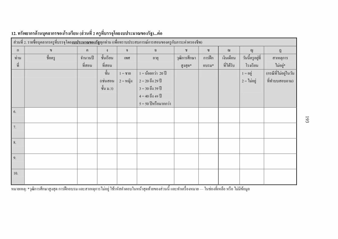
193

12. ทรพยากรดานบคลากรของโรงเรยน (สวนท 2 ครทบรรจโดยงบประมาณของรฐ)...ตอ สวนท 2. รายชอบคลากรครทบรรจโดยงบประมาณของรฐทกทาน (เพอทราบประสบการณการสอนของครกบภาระคาครองชพ) ก ข ค ง จ ฉ ช ซ ฌ ญ ฎ

ทานท

ชอคร จ านวนปทสอน

ชนเรยน ทสอน

เพศ อาย วฒการศกษาสงสด*

การฝก อบรม*

เงนเดอน

ทไดรบ วนนครอยทโรงเรยน

สาเหตการ ไมอย*

ชน (เชนสอนชน ม.3)

1 = ชาย 2 = หญง

1 = นอยกวา 20 ป 2 = 20 ถง 29 ป 3 = 30 ถง 39 ป 4 = 40 ถง 49 ป 5 = 50 ปหรอมากกวา

1 = อย 2 = ไมอย

(กรณทไมอยในวน ทท าบบสอบถาม)

6.

7.

8.

9.

10.

หมายเหต: *วฒการศกษาสงสด การฝกอบรม และสาเหตการไมอย ใชรหสค าตอบในหนาสดทายของสวนน และท าเครองหมาย — ในชองทเหลอ หรอ ไมมขอมล

194

12. ทรพยากรดานบคลากรของโรงเรยน (สวนท 2 ครทบรรจโดยงบประมาณของรฐ)...ตอ สวนท 2. รายชอบคลากรครทบรรจโดยงบประมาณของรฐทกทาน (เพอทราบประสบการณการสอนของครกบภาระคาครองชพ) ก ข ค ง จ ฉ ช ซ ฌ ญ ฎ

ทานท

ชอคร จ านวนปทสอน

ชนเรยน ทสอน

เพศ อาย วฒการศกษาสงสด*

การฝก อบรม*

เงนเดอน

ทไดรบ วนนครอยทโรงเรยน

สาเหตการ ไมอย*

ชน (เชนสอนชน ม.3)

1 = ชาย 2 = หญง

1 = นอยกวา 20 ป 2 = 20 ถง 29 ป 3 = 30 ถง 39 ป 4 = 40 ถง 49 ป 5 = 50 ปหรอมากกวา

1 = อย 2 = ไมอย

(กรณทไมอยในวน

ทท าแบบสอบถาม)

11.

12.

13.

14.

15.

หมายเหต: *วฒการศกษาสงสด การฝกอบรม และสาเหตการไมอย ใชรหสค าตอบในหนาสดทายของสวนน และท าเครองหมาย — ในชองทเหลอ หรอ ไมมขอมล

195

12. ทรพยากรดานบคลากรของโรงเรยน (สวนท 2 ครทบรรจโดยงบประมาณของรฐ)...ตอ สวนท 2. รายชอบคลากรครทบรรจโดยงบประมาณของรฐทกทาน (เพอทราบประสบการณการสอนของครกบภาระคาครองชพ) ก ข ค ง จ ฉ ช ซ ฌ ญ ฎ

ทานท

ชอคร จ านวนปทสอน

ชนเรยน ทสอน

เพศ อาย วฒการศกษาสงสด*

การฝก อบรม*

เงนเดอน

ทไดรบ วนนครอยทโรงเรยน

สาเหตการ ไมอย*

ชน (เชนสอนชน ม.3)

1 = ชาย 2 = หญง

1 = นอยกวา 20 ป 2 = 20 ถง 29 ป 3 = 30 ถง 39 ป 4 = 40 ถง 49 ป 5 = 50 ปหรอมากกวา

1 = อย 2 = ไมอย

(กรณทไมอยในวน

ทท าแบบสอบถาม)

16.

17.

18.

19.

20.

หมายเหต: *วฒการศกษาสงสด การฝกอบรม และสาเหตการไมอย ใชรหสค าตอบในหนาสดทายของสวนน และท าเครองหมาย — ในชองทเหลอ หรอ ไมมขอมล

196

12. ทรพยากรดานบคลากรของโรงเรยน (สวนท 2 ครทบรรจโดยงบประมาณของรฐ)...ตอ สวนท 2. รายชอบคลากรครทบรรจโดยงบประมาณของรฐทกทาน (เพอทราบประสบการณการสอนของครกบภาระคาครองชพ) ก ข ค ง จ ฉ ช ซ ฌ ญ ฎ

ทานท

ชอคร จ านวนปทสอน

ชนเรยน ทสอน

เพศ อาย วฒการศกษาสงสด*

การฝก อบรม*

เงนเดอน

ทไดรบ วนนครอยทโรงเรยน

สาเหตการ ไมอย*

ชน (เชนสอนชน ม.3)

1 = ชาย 2 = หญง

1 = นอยกวา 20 ป 2 = 20 ถง 29 ป 3 = 30 ถง 39 ป 4 = 40 ถง 49 ป 5 = 50 ปหรอมากกวา

1 = อย 2 = ไมอย

(กรณทไมอยในวน

ทท าแบบสอบถาม)

21.

22.

23.

24.

25.

หมายเหต: *วฒการศกษาสงสด การฝกอบรม และสาเหตการไมอย ใชรหสค าตอบในหนาสดทายของสวนน และท าเครองหมาย — ในชองทเหลอ หรอ ไมมขอมล

197

1. รหสค าตอบเกยวกบวฒการศกษาสงสด

1. อนปรญญา 2. ปรญญาตรดานการศกษา 3. ปรญญาตรดานอนๆ 4. ปรญญาโทดานการศกษา 5. ปรญญาโทดานอนๆ 6. ปรญญาเอกดานการศกษา 7. ปรญญาเอกดานอนๆ

2. รหสค าตอบเกยวกบการฝกอบรม 1. ฝกอบรมดานการเรยนการสอน 2. ฝกอบรมหลกสตรดานการบรหาร 3. ไมเคยเขาฝกอบรม 4. อนๆ ระบ _____________________________________

3. รหสค าตอบเกยวกบสาเหตการไมอย 1. ลาราชการโดยไดรบอนญาตในวนน

2. ลาโดยไมทราบสาเหตในวนน 3. อนๆระบ______________________________________

198

13. ขอมลครผสอนในชวงชนประถมศกษา 1 ทานและครผสอนชนมธยมศกษาปท 1 หรอปท 2 เลอกโดยสม 1 ทาน (ตอบโดย ผอ./รอง ผอ. โรงเรยน) ขอมลปจจบนเกยวกบครผสอนชนประถมศกษาจ านวน 1 ทานและครทสอนมธยมศกษาปท 1 หรอ 2 จ านวน 1 ทาน (โดยสม) ก ข รหส / หนวยค าตอบ

ครผสอนชนประถมศกษา 1 ทาน ครผสอนชนมธยมศกษา 1 ทาน 1. ชอ ชอ

2. แฟมประวต (ก.พ.7) หมายเลขอางอง

3. วฒการศกษาสงสดของคร 1 = อนปรญญา 2 = ปรญญาตรดานการศกษา 3 = ปรญญาตรดานอนๆ 4 = ปรญญาโทดานการศกษา 5 = ปรญญาโทดานอนๆ 6 = ปรญญาเอกดานการศกษา 7 = ปรญญาเอกดานอนๆ 88 = อนๆระบ _______________________________

4. การเขารบการฝกอบรม... (ตอบไดมากกวา 1 ขอ)

1 = ดานการเรยนการสอน 2 = หลกสตรดานการบรหาร 88 = อนๆระบ ______________________________

5. ครมภมล าเนาในต าบลน 1 = ม

2 = ไมม 6. ครมภมล าเนาในอ าเภอน

7. ครมภมล าเนาในจงหวดน

199

ก ข รหส / หนวยค าตอบ

ครผสอนชนประถมศกษา 1 ทาน ครผสอนชนประถมศกษาจ านวน 1 ทาน ครผสอนชนมธยมศกษา 1 ทาน 8. จ านวนปทงหมดทบรรจเขาท างานเปนคร จ านวนป 9. จ านวนปทงหมดทสอนท ร.ร. น 10. การรายงานตวเขาท างาน

รายงานในวน / เดอน / ป

______ / _______ / _______ 11. ในวนทตอบแบบสอบถาม ครทานนอยท

โรงเรยน 1 = อยท ร.ร.

2 = ไมอยท ร.ร. 12. ถาไมอย จ านวนวนทไมอย วนท าการ 13. เหตทไมอย 1 ไดรบอนญาตใหลาตาม

ระเบยบ 2 ลาโดยไมทราบสาเหต 3. อนๆระบ_________

14. จ านวนวนทงหมดทลาโดยไดรบอนญาต จ านวนวน 15. จ านวนวนทงหมดทลาโดยไมทราบสาเหต 16. จ านวนวนทงหมดทลาโดยเหตอนๆในขอ 13

200

17. ครไดรบค าสงใหไปอบรมในระหวาง

ปงบประมาณ 2549 1 = ไดรบค าสง

2 = ไมไดรบค าสง

18. ถาไดรบ เรองทอบรม ระบเรอง 19. จงหวดทไปอบรม ระบจงหวด 20. เวลาทใชอบรม จ านวน (วน) 21. หนวยงานผอนมตงบประมาณ ระบหนวยงาน

ก ข รหส / หนวยค าตอบ ครผสอนชนประถมศกษา 1 ทาน ครผสอนชนมธยมศกษา 1 ทาน

22. ครไดรบค าสงใหไปอบรมในระหวาง ปงบประมาณ 2550

1 = ไดรบค าสง 2 = ไมไดรบค าสง

23. ถาไดรบ เรองทอบรม ระบเรอง 24. จงหวดทไปอบรม ระบจงหวด 25. เวลาทใชอบรม จ านวน (วน) 26. หนวยงานผอนมตงบประมาณ ระบหนวยงาน

201

27. ครพกอยในบานพกของ ร.ร.

(ถาไมอย: ขามไปท าขอ 30) 1 = อย

2 = ไมไดอย

28. ถาอย ผทเปนเจาของบานพก 1 = ทราชพสด 2 = ทเทศบาล, อบต., อบจ. 3 = ทของเอกชน 4 = ทของวด 88 = อนๆระบ_______

29. คาเชาบานตอเดอน บาท 0 = ไมมคาเชาบาน 30. ลกษณะของบานพก 1 = สรางเพอใชเปนบานพก

ถาวร 2 = ใชอาคารอนๆของ ร.ร. เปนบานพก

31. เงนเดอนทไดรบตอเดอน บาท

32. จ านวนเงนทหกจากเงนเดอน

33. เงนเดอนทไดรบสทธ

ก ข รหส / หนวยค าตอบ ครผสอนชนประถมศกษา 1 ทาน ครผสอนชนมธยมศกษา 1 ทาน

34. วธจายเงนเดอนของโรงเรยน 1 = เชค 2 = เงนสด 3 = ผานบญชธนาคาร

35. เวลาจายเงนเดอนในเดอนทผานมา วนท / เดอน

202

36. ครไดรบเงนเพมพเศษตามสทธ

ในปงบประมาณ 2549 1 = ได

2 = ไมได 37. ถาได

ชนดของเงนเพมพเศษ

1 = เบยกนดาร 2 = คาเสยงภย, 3 = คาเชาบาน 4 = เงนวทยฐานะ 88=อนๆ ระบ _______

38. จ านวนเงนเพมพเศษทไดรบ ทงสนในปงบประมาณ 2549

บาท

39. ครไดรบเงนเพมพเศษตามสทธ ในปงบประมาณ 2550

1 = ได 2 = ไมได

40. ถาได

ชนดของเงนเพมพเศษ

1 = เบยกนดาร, 2 = คาเสยงภย, 3 = คาเชาบาน 4 = เงนวทยฐานะ 88=อนๆ ระบ _______

41. จ านวนเงนเพมพเศษทไดรบ ทงสนในปงบประมาณ 2550

บาท

203

14. ผลการประเมนผลสมฤทธทางการเรยนเฉลยของนกเรยนชวงชนทหนงและชวงชนทสาม

ชวงชนทหนง (ป.1 – ป.3)

วชา คะแนนผลสมฤทธทางการเรยน

ปการศกษา 2549 ปการศกษา 2550

คะแนนเฉลยของโรงเรยน คะแนนเฉลยทวประเทศ (ระดบชาต)

คะแนนเฉลยของโรงเรยน คะแนนเฉลยทวประเทศ (ระดบชาต)

1. คณตศาสตร

2. ภาษาไทย

ชวงชนทสาม (ม.1 – ม.3)

วชา คะแนนผลสมฤทธทางการเรยน

ปการศกษา 2549 ปการศกษา 2550

คะแนนเฉลยของโรงเรยน คะแนนเฉลยทวประเทศ (ระดบชาต)

คะแนนเฉลยของโรงเรยน คะแนนเฉลยทวประเทศ (ระดบชาต)

1. คณตศาสตร

2. วทยาศาสตร

3. ภาษาองกฤษ

4. ภาษาไทย

5. สงคมศกษา ศาสนา และวฒนธรรม

204

15. จ านวนทรพยากรทางการศกษาทงหมดในโรงเรยน ในปการศกษาตางๆ

1. จ านวนหองเรยนในแตละชนเรยน จ านวนหองเรยน

ปการศกษา 2549 ปการศกษา 2550 ปการศกษา 2551

กอนประถมศกษาปท 1 (อนบาล)

กอนประถมศกษาปท 2 (อนบาล)

กอนประถมศกษาปท 3 (อนบาล)

ประถมศกษาปท 1

ประถมศกษาปท 2

ประถมศกษาปท 3

ประถมศกษาปท 4

ประถมศกษาปท 5

ประถมศกษาปท 6

มธยมศกษาปท 1

มธยมศกษาปท 2

มธยมศกษาปท 3

รวม

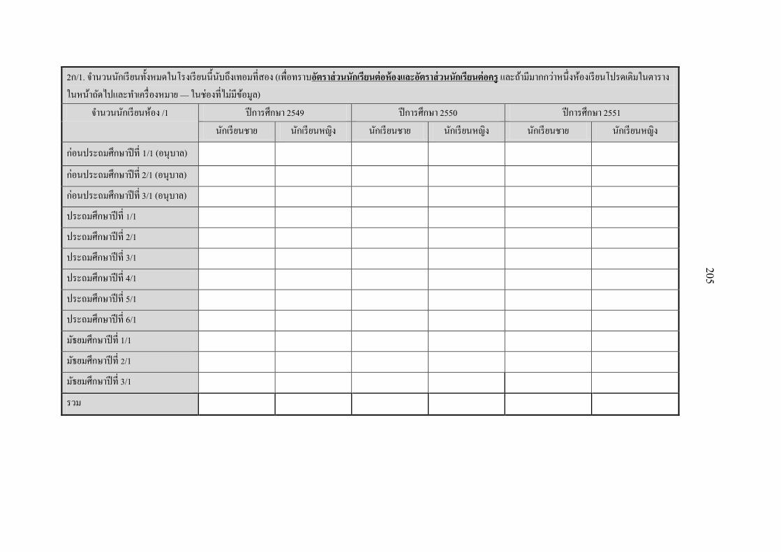
205

2ก/1. จ านวนนกเรยนทงหมดในโรงเรยนนนบถงเทอมทสอง (เพอทราบอตราสวนนกเรยนตอหองและอตราสวนนกเรยนตอคร และถามมากกวาหนงหองเรยนโปรดเตมในตารางในหนาถดไปและท าเครองหมาย — ในชองทไมมขอมล)

จ านวนนกเรยนหอง /1 ปการศกษา 2549 ปการศกษา 2550 ปการศกษา 2551 นกเรยนชาย นกเรยนหญง นกเรยนชาย นกเรยนหญง นกเรยนชาย นกเรยนหญง

กอนประถมศกษาปท 1/1 (อนบาล)

กอนประถมศกษาปท 2/1 (อนบาล)

กอนประถมศกษาปท 3/1 (อนบาล)

ประถมศกษาปท 1/1

ประถมศกษาปท 2/1

ประถมศกษาปท 3/1

ประถมศกษาปท 4/1

ประถมศกษาปท 5/1

ประถมศกษาปท 6/1

มธยมศกษาปท 1/1

มธยมศกษาปท 2/1

มธยมศกษาปท 3/1

รวม

206

2ก/2. จ านวนนกเรยนทงหมดในโรงเรยนนนบถงเทอมทสอง (เพอทราบอตราสวนนกเรยนตอหองและอตราสวนนกเรยนตอคร)

จ านวนนกเรยนหอง /2 (ถาม) ปการศกษา 2549 ปการศกษา 2550 ปการศกษา 2551 นกเรยนชาย นกเรยนหญง นกเรยนชาย นกเรยนหญง นกเรยนชาย นกเรยนหญง

กอนประถมศกษาปท 1/2 (อนบาล)

กอนประถมศกษาปท 2/2 (อนบาล)

กอนประถมศกษาปท 3/2 (อนบาล)

ประถมศกษาปท 1/2

ประถมศกษาปท 2/2

ประถมศกษาปท 3/2

ประถมศกษาปท 4/2

ประถมศกษาปท 5/2

ประถมศกษาปท 6/2

มธยมศกษาปท 1/2

มธยมศกษาปท 2/2

มธยมศกษาปท 3/2

รวม

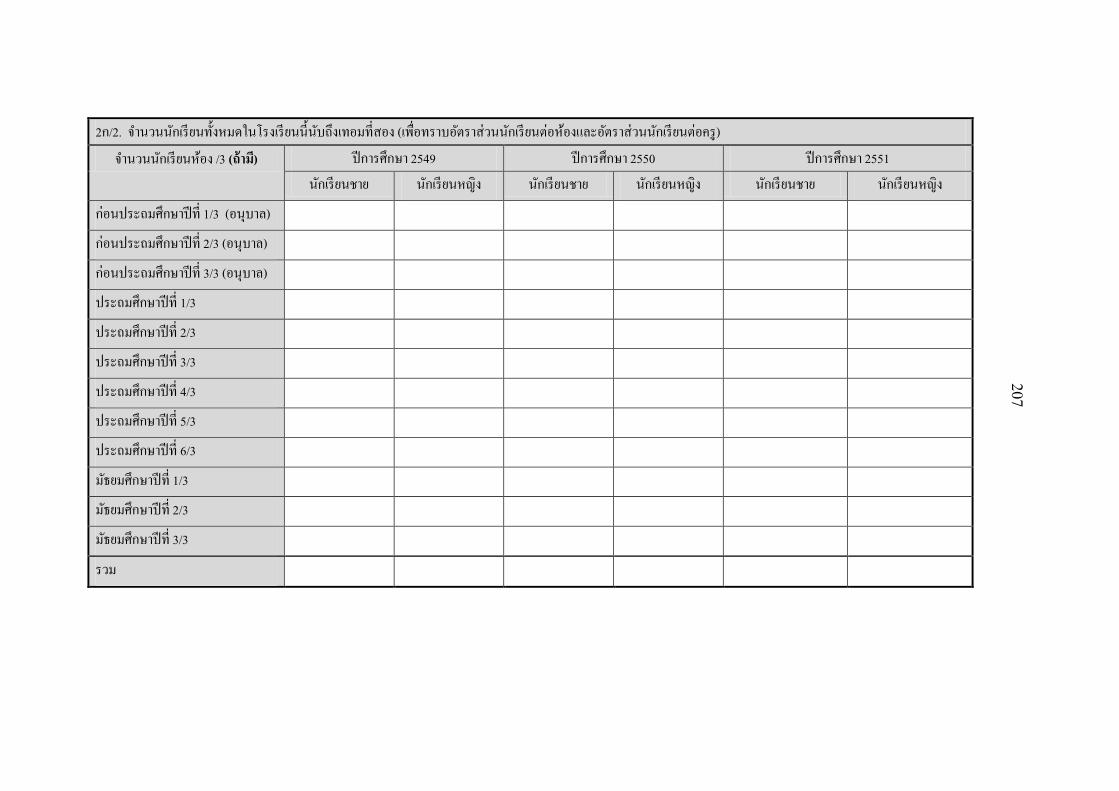
207

2ก/2. จ านวนนกเรยนทงหมดในโรงเรยนนนบถงเทอมทสอง (เพอทราบอตราสวนนกเรยนตอหองและอตราสวนนกเรยนตอคร) จ านวนนกเรยนหอง /3 (ถาม) ปการศกษา 2549 ปการศกษา 2550 ปการศกษา 2551

นกเรยนชาย นกเรยนหญง นกเรยนชาย นกเรยนหญง นกเรยนชาย นกเรยนหญง

กอนประถมศกษาปท 1/3 (อนบาล)

กอนประถมศกษาปท 2/3 (อนบาล)

กอนประถมศกษาปท 3/3 (อนบาล)

ประถมศกษาปท 1/3

ประถมศกษาปท 2/3

ประถมศกษาปท 3/3

ประถมศกษาปท 4/3

ประถมศกษาปท 5/3

ประถมศกษาปท 6/3

มธยมศกษาปท 1/3

มธยมศกษาปท 2/3

มธยมศกษาปท 3/3

รวม

208

3. จ านวนนกเรยนทส าเรจการศกษาในชนทผานมา แตไมเรยนตอในโรงเรยนนในปการศกษาน (เพอทราบอตราการลาออก) ชนเรยน ปการศกษา 2549 ปการศกษา 2550 ปการศกษา 2551

นกเรยนชาย นกเรยนหญง นกเรยนชาย นกเรยนหญง นกเรยนชาย นกเรยนหญง

กอนประถมศกษาปท 1 (อนบาล)

กอนประถมศกษาปท 2 (อนบาล)

กอนประถมศกษาปท 3 (อนบาล)

ประถมศกษาปท 1

ประถมศกษาปท 2

ประถมศกษาปท 3

ประถมศกษาปท 4

ประถมศกษาปท 5

ประถมศกษาปท 6

มธยมศกษาปท 1

มธยมศกษาปท 2

มธยมศกษาปท 3

รวม

209

4. จ านวนนกเรยนทเรยนตอในชนเรยนทสงขนของโรงเรยนนโดยรวม (เพอทราบอตราการเรยนตอ)

ชนเรยน ปการศกษา 2549 ปการศกษา 2550 ปการศกษา 2551 รอยละของ นกเรยนชาย

รอยละของ นกเรยนหญง

รอยละของ นกเรยนชาย

รอยละของ นกเรยนหญง

รอยละของ นกเรยนชาย

รอยละของ นกเรยนหญง

กอนประถมศกษาปท 3 (อนบาล)

ประถมศกษาปท 6

มธยมศกษาปท 3

รวม

210

5ก. จ านวนนกเรยนในปจจบนทงหมดทมาเรยนในวนนเมอสปดาหทแลว (เพอทราบอตราการขาดเรยน)

ชนเรยน นกเรยนหอง /1 นกเรยนหอง /2 (ถาม) นกเรยนหอง /3 (ถาม) นกเรยนชาย นกเรยนหญง นกเรยนชาย นกเรยนหญง นกเรยนชาย นกเรยนหญง

กอนประถมศกษาปท 1 (อนบาล)

กอนประถมศกษาปท 2 (อนบาล)

กอนประถมศกษาปท 3 (อนบาล)

ประถมศกษาปท 1

ประถมศกษาปท 2

ประถมศกษาปท 3

ประถมศกษาปท 4

ประถมศกษาปท 5

ประถมศกษาปท 6

มธยมศกษาปท 1

มธยมศกษาปท 2

มธยมศกษาปท 3

รวม

211

ขอ ค าถาม ค าตอบ รหส/หนวย

ปการศกษา 2549 ปการศกษา 2550 ปการศกษา 2551 6. โรงเรยนไมสามารถรบนกเรยนไดเพราะ

หองเรยนเตมในปการศกษา.... 1 = ใช

2 = ไมใช 7. จ านวนนกเรยนทโรงเรยนไมสามารถรบ

เขาเรยนได จ านวน

8. หนงสอเรยนวชาคณตศาสตรชนประถมศกษา (เพอทราบทรพยากรทางการศกษาเปรยบเทยบกบผลสมฤทธทางการศกษา และถาไมมขอมลโปรดท าเครองหมาย —)

ปงบประมาณ 2549 ปงบประมาณ 2550

จ านวนทมอยกอน ในโรงเรยน (เลม)

จ านวนทไดรบเพมในปงบประมาณ 2549 จ านวนทมอยกอน ในโรงเรยน (เลม)

จ านวนทไดรบเพมในปงบประมาณ 2550 โดยไมตองซอ โดยตองซอเพม โดยไมตองซอ โดยตองซอเพม

ก. ข. ค. ง. จ. ฉ.

ประถมศกษาปท 1

ประถมศกษาปท 2

ประถมศกษาปท 3

ประถมศกษาปท 4

ประถมศกษาปท 5

ประถมศกษาปท 6

รวม

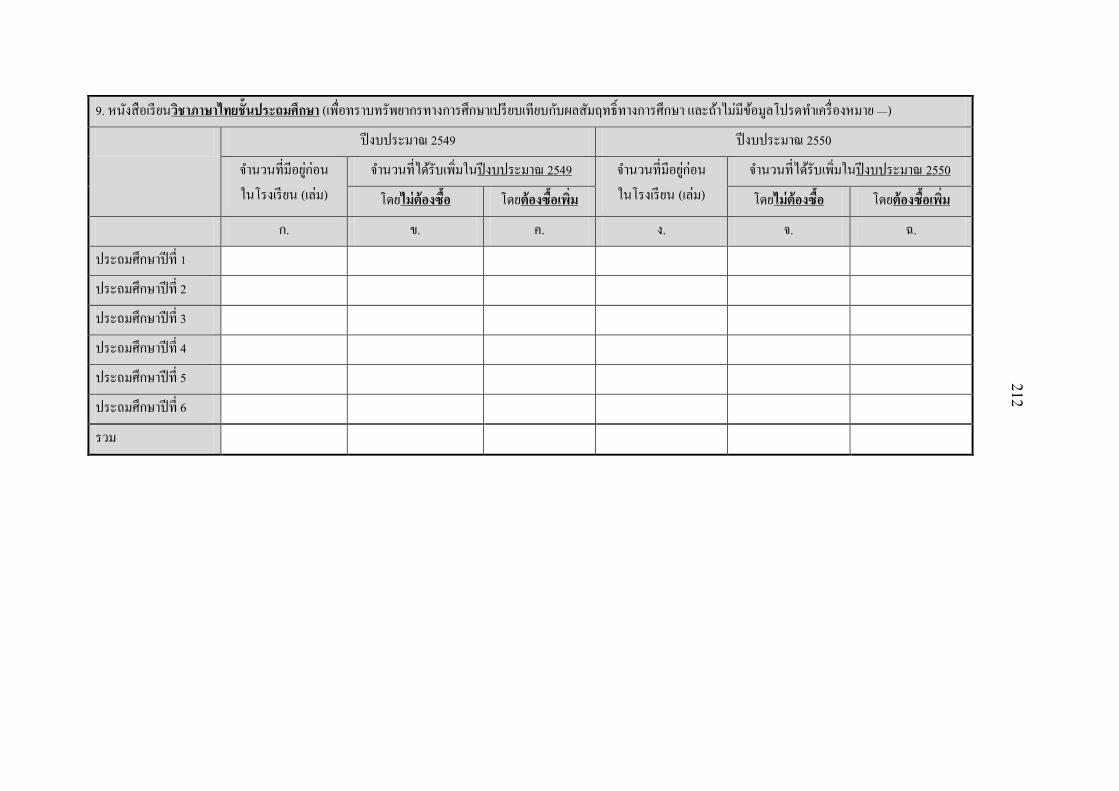
212

9. หนงสอเรยนวชาภาษาไทยชนประถมศกษา (เพอทราบทรพยากรทางการศกษาเปรยบเทยบกบผลสมฤทธทางการศกษา และถาไมมขอมลโปรดท าเครองหมาย —)

ปงบประมาณ 2549 ปงบประมาณ 2550

จ านวนทมอยกอน ในโรงเรยน (เลม)

จ านวนทไดรบเพมในปงบประมาณ 2549 จ านวนทมอยกอน ในโรงเรยน (เลม)

จ านวนทไดรบเพมในปงบประมาณ 2550

โดยไมตองซอ โดยตองซอเพม โดยไมตองซอ โดยตองซอเพม

ก. ข. ค. ง. จ. ฉ.

ประถมศกษาปท 1

ประถมศกษาปท 2

ประถมศกษาปท 3

ประถมศกษาปท 4

ประถมศกษาปท 5

ประถมศกษาปท 6

รวม

213

10. หนงสอเรยนวชาคณตศาสตรชนมธยมศกษาตอนตน (เพอทราบทรพยากรทางการศกษาเปรยบเทยบกบผลสมฤทธทางการศกษา และถาไมมขอมลโปรดท าเครองหมาย —)

ปงบประมาณ 2549 ปงบประมาณ 2550

จ านวนทมอยกอน ในโรงเรยน (เลม)

จ านวนทไดรบเพมในปงบประมาณ 2549 จ านวนทมอยกอน ในโรงเรยน (เลม)

จ านวนทไดรบเพมในปงบประมาณ 2550 โดยไมตองซอ โดยตองซอเพม โดยไมตองซอ โดยตองซอเพม

ก. ข. ค. ง. จ. ฉ. มธยมศกษาปท 1

มธยมศกษาปท 2

มธยมศกษาปท 3

รวม

11. หนงสอเรยนวชาวทยาศาสตรชนมธยมศกษาตอนตน (เพอทราบทรพยากรทางการศกษาเปรยบเทยบกบผลสมฤทธทางการศกษา และถาไมมขอมลโปรดท าเครองหมาย —)

ปงบประมาณ 2549 ปงบประมาณ 2550

จ านวนทมอยกอน ในโรงเรยน (เลม)

จ านวนทไดรบเพมในปงบประมาณ 2549 จ านวนทมอยกอน ในโรงเรยน (เลม)

จ านวนทไดรบเพมในปงบประมาณ 2550 โดยไมตองซอ โดยตองซอเพม โดยไมตองซอ โดยตองซอเพม

ก. ข. ค. ง. จ. ฉ. มธยมศกษาปท 1

มธยมศกษาปท 2

มธยมศกษาปท 3

รวม

214

12. หนงสอเรยนวชาภาษาไทยชนมธยมศกษาตอนตน (เพอทราบทรพยากรทางการศกษาเปรยบเทยบกบผลสมฤทธทางการศกษา และถาไมมขอมลโปรดท าเครองหมาย —)

ปงบประมาณ 2549 ปงบประมาณ 2550

จ านวนทมอยกอน ในโรงเรยน (เลม)

จ านวนทไดรบเพมในปงบประมาณ 2549 จ านวนทมอยกอน ในโรงเรยน (เลม)

จ านวนทไดรบเพมในปงบประมาณ 2550 โดยไมตองซอ โดยตองซอเพม โดยไมตองซอ โดยตองซอเพม

ก. ข. ค. ง. จ. ฉ.

มธยมศกษาปท 1

มธยมศกษาปท 2

มธยมศกษาปท 3

รวม

13. หนงสอเรยนวชาภาษาองกฤษชนมธยมศกษา (เพอทราบทรพยากรทางการศกษาเปรยบเทยบกบผลสมฤทธทางการศกษา และถาไมมขอมลโปรดท าเครองหมาย —)

ปงบประมาณ 2549 ปงบประมาณ 2550 จ านวนทมอยกอน ในโรงเรยน (เลม)

จ านวนทไดรบเพมในปงบประมาณ 2549 จ านวนทมอยกอน ในโรงเรยน (เลม)

จ านวนทไดรบเพมในปงบประมาณ 2550 โดยไมตองซอ โดยตองซอเพม โดยไมตองซอ โดยตองซอเพม

ก. ข. ค. ง. จ. ฉ.

มธยมศกษาปท 1

มธยมศกษาปท 2

มธยมศกษาปท 3

รวม

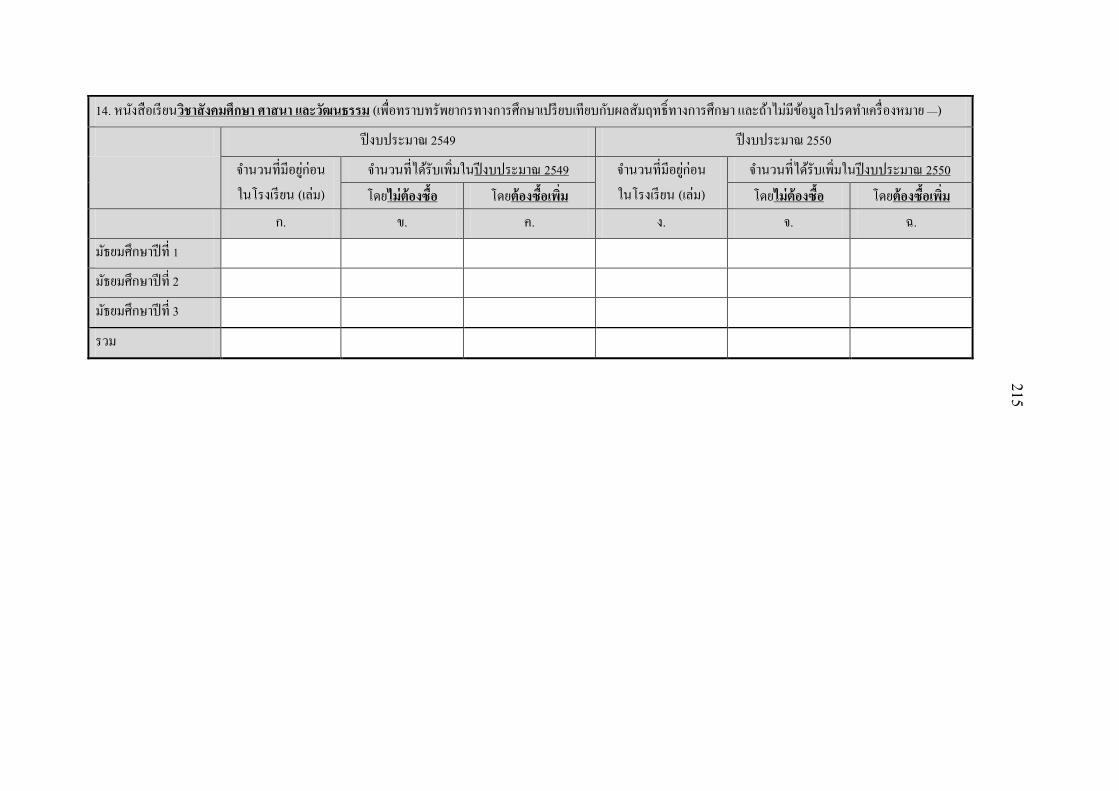
215

14. หนงสอเรยนวชาสงคมศกษา ศาสนา และวฒนธรรม (เพอทราบทรพยากรทางการศกษาเปรยบเทยบกบผลสมฤทธทางการศกษา และถาไมมขอมลโปรดท าเครองหมาย —)

ปงบประมาณ 2549 ปงบประมาณ 2550

จ านวนทมอยกอน ในโรงเรยน (เลม)

จ านวนทไดรบเพมในปงบประมาณ 2549 จ านวนทมอยกอน ในโรงเรยน (เลม)

จ านวนทไดรบเพมในปงบประมาณ 2550 โดยไมตองซอ โดยตองซอเพม โดยไมตองซอ โดยตองซอเพม

ก. ข. ค. ง. จ. ฉ.

มธยมศกษาปท 1

มธยมศกษาปท 2

มธยมศกษาปท 3

รวม

216

แบบสอบถามผอ านวยการส านกงานเขตพนทการศกษา (สพท.)

217

แบบสอบถามส าหรบวทยานพนธปรญญาเอกสาขาเศรษฐศาสตรเรอง

“School Expenditure Leakage and Efficiency: The Case of Thai Compulsory Education”

ค าชแจง 1. โปรดตอบค าถามโดยลงรหสค าตอบ/ค าตอบลงในชองวางโดยใชปากกา ดงตวอยาง ขอ ค าถาม ค าตอบ รหส / หนวยค าตอบ

15. ถามการสนบสนน: โดยปกตแลว ประเภทของการสนบสนนเพมเตม

3 1 = เงนงบประมาณ 2 = จ านวนคร 3 = อปกรณการเรยนการสอน, ครภณฑตางๆ 4 = อนๆโปรดระบ ______________________

16. จ านวนครงทส านกงานเขตพนทการศกษา (สพท.) จดการประชมกบผอ านวยการโรงเรยนในเรองการบรหารการศกษา

2 1 = เดอนละหนงครง 2 = สองถงสามเดอนครง 3 = ภาคการศกษาละหนงครง 4 = ปการศกษาละครง

2. ในขอทไมมรหสค าตอบ โปรดเตมค าตอบในชองวางหรอเนอทวาง 3. โปรดตอบค าถามทกขอ โดยเฉพาะงบประมาณของโรงเรยน เพอทจะสามารถน าขอมลไปค านวณทางสถตและแปลผลตามหลกวชาการ 4. โปรดท าเครองหมาย —ในชองทไมมขอมล

5. ขอมลทงหมดเปนความลบและใชเพอการศกษาวจยเทานน 6. วทยานพนธนสวนหนงจะลงพมพในวารสารวชาการ(ตามขอก าหนดของส านกงานคณะกรรมการการอดมศกษา)

7. ผวจยขอขอบคณทกทานอยางสงทอนเคราะหขอมลเพอเปนประโยชนในทางวชาการ 8. ผวจยจะเดนทางเขาไปรบแบบสอบถามในชวงเวลา 2- 4 สปดาหภายหลงจากไดรบแบบสอบถาม

ชอผวจย นายจระเดช ทศยาพนธ นกศกษาปรญญาเอกคณะพฒนาการเศรษฐกจ สถาบนบณฑตพฒนบรหารศาสตร (นดา) โทร. 081 1700051 emails: jiradate.t@hotmail.com, jiradate.t@gmail.com

218

ชดแบบสอบถามส านกงานเขตพนทการศกษา

1. ขอมลพนฐาน ส านกงานเขตพนทการศกษา _________________________________

ขอ ค าถาม ค าตอบ รหส / หนวยค าตอบ

1. ชอจงหวด โปรดระบจงหวด 2. ส านกงานเขตพนทการศกษา (สพท.) เขตพนทการศกษา 3. วน/เดอน/ปทตอบแบบสอบถาม / / 2551 วน / เดอน / ป

4. ผตอบแบบสอบถาม ระบชอ 5. เพศ 1 = ชาย 2 = หญง 6. สถานภาพ 1 = โสด

2 = สมรส 3 = หยาราง

7. วฒการศกษาของทาน

1 = อนปรญญา 2 = ปรญญาตรดานการศกษา 3 = ปรญญาตรดานอนๆ 4 = ปรญญาโทดานการศกษา 5 = ปรญญาโทดานอนๆ 6 = ปรญญาเอกดานการศกษา 7 = ปรญญาเอกดานอนๆ

88 = อนๆ ระบ __________________________ 8. ทานไดรบการฝกอบรม...

(ตอบไดมากกวา 1 ขอ) 1 = ดานการเรยนการสอน

2 = หลกสตรดานการบรหาร 88 = อนๆ ระบ_________________________

219

9. จ านวนผอ านวยการส านกงานเขตพนทการศกษา (สพท.)

ทไดรบการแตงตงในเขตพนทนในรอบหาปทผานมา 1 = หนง

2 = สอง 3 = สาม 4 = มากกวาส

10.

ใน สพท. นมต าแหนงตามกรอบอตราก าลงทงหมดกทาน

จ านวนกรอบอตราก าลง (ต าแหนง)

11. ขณะนทกต าแหนงไดรบการบรรจทงหมด 1 = บรรจทงหมด 2 = ยงบรรจไมหมด

12. ถายงบรรจไมหมด: จ านวนทยงไมไดบรรจบคลากร

จ านวน (คน)

13. ทานคดวาโรงเรยนใดในพนทนทมความขาดแคลนทรพยากรในดานตางๆมากทสด (ตอบไดหลายโรงเรยน)

ชอโรงเรยน

14. ทานไดจดสรรการสนบสนนเพมเตมใหโรงเรยนเหลาน 1 = สนบสนน 2 = ไมไดสนบสนน

15. ถามการสนบสนน: โดยปกตแลว ประเภทของการสนบสนนเพมเตม

1 = เงนงบประมาณ 2 = จ านวนคร 3 = อปกรณการเรยนการสอน, ครภณฑตางๆ 4 = อนๆโปรดระบ ______________________

220

16. จ านวนครงทส านกงานเขตพนทการศกษา (สพท.) จดการ

ประชมกบผอ านวยการโรงเรยนในเรองการบรหารการศกษา 1 = เดอนละหนงครง

2 = สองถงสามเดอนครง 3 = ภาคการศกษาละหนงครง 4 = ปการศกษาละครง

17. โปรดเรยงล าดบความส าคญของหนวยงานหรอบคคลทม อทธพลตอการตดสนใจในการบรหารการศกษาใน เขตพนทการศกษา (ตอบ 3 ล าดบ)

ล าดบท 1.

1 = ส านกงานคณะกรรมการการศกษาขนพนฐาน (สพฐ.) 2 = ผอ านวยการส านกงานเขตพนทการศกษา (สพท.) 3 = คณะกรรมการส านกงานเขตพนทการศกษา 4 = คณะกรรมการสถานศกษาขนพนฐาน 5 = สมาคมครและผปกครอง 6 = ผอ านวยการโรงเรยน 7 = ผน าการเมองทองถน 88 = อนๆ ระบ ____________________________________

ล าดบท 2.

ล าดบท 3.

18. สพท. มการบรหารในรปคณะกรรมการ (ถาไมม ขามไปท าสวนท 2.)

1 = ม 2 = ไมม

221

19. ถาบรหารในรปคณะกรรมการ, ในปงบประมาณ 2549 มการ

ประชมทงหมดกครงและเมอใด จ านวนครง

ครงท ครงท ครงท ครงท

วน / เดอน / ป ทประชม

20. ถาบรหารในรปคณะกรรมการ, ในปงบประมาณ 2550 มการประชมทงหมดกครงและเมอใด

จ านวนครง ครงท

ครงท

ครงท

ครงท

วน / เดอน / ป ทประชม

222

21. ทานคดวาการประชมมประสทธผล 1 = มประสทธผลมาก

2 = มประสทธผลปานกลาง

3 = ไมมประสทธผลเลย

88 = อนๆ ระบ

_________________________

99 = ไมมความคดเหน

22. จ านวนคณะกรรมการฯทมอยในขณะน

จ านวน (คน)

23. สมาชกของคณะกรรมการฯ สพท. เปนตวแทนจากกลมใด

โปรดระบกลมตวแทนและจ านวนผแทน

จ านวนตวแทนชาย จ านวนตวแทนหญง

จากผบรหารโรงเรยน

จากผแทนครและบคลากรในโรงเรยน

จากผแทนผปกครอง

จากผแทนองคกรปกครองสวนทองถน

จากผทรงคณวฒ

จากผแทนศษยเกา

จากผแทนองคกรศาสนา

จากองคกรชมชน ระบ ___________________

อนๆระบ __________________________

223

2. ทรพยากรทางการศกษา (เพอเปนตวแปรเชงสถต)

24. จ านวนแยกตามประเภทโรงเรยนในเขตพนทการศกษาน ปงบประมาณ 2549 ปงบประมาณ 2550 ปงบประมาณ 2551 หนวย

24ก. โรงเรยนขยายโอกาสทางการศกษา จ านวนโรงเรยน 24ข. โรงเรยนประถมศกษา 24ค. โรงเรยนมธยมศกษา 24ง. โรงเรยนมธยมศกษาเอกชน 24จ. โรงเรยนอาชวะศกษา 24ฉ. โรงเรยนศกษาผใหญ 24ช. อนๆ ระบ

________________________________________

25. จ านวนโรงเรยนในเขตพนทนทปดชวคราวในขณะน 25ก. โรงเรยนขยายโอกาสทางการศกษา จ านวนโรงเรยน

0 = ไมมโรงเรยนใดปด 25ข. โรงเรยนประถมศกษา

25ค. โรงเรยนมธยมศกษา

25ง. โรงเรยนมธยมศกษาเอกชน

25จ. โรงเรยนอาชวะศกษา

25ฉ. โรงเรยนศกษาผใหญ

25ช. อนๆ ระบ

_______________________________

224

ปงบประมาณ 2549 ปงบประมาณ 2550 ปงบประมาณ 2551 หนวย 26. จ านวนอตราครทงหมดของโรงเรยนขยายโอกาสทาง

การศกษาทงหมดในเขตพนทนในปงบประมาณ.. จ านวน (คน)

27. จ านวนครทยงไมไดบรรจตามอตราในโรงเรยนขยายโอกาสทางการศกษาทงหมดในเขตพนทนในขณะน

ปงบประมาณ 2549 ปงบประมาณ 2550 ปงบประมาณ 2551 หนวย ชาย หญง ชาย หญง ชาย หญง

28. ผอ านวยการโรงเรยนขยายโอกาสทางการศกษาทงหมดในเขตพนทนเปนชายหรอหญงจ านวนกทาน…

จ านวน (คน)

225

3. การจดท างบประมาณ (เพอเปนขอมลเชงสถต) ขอ ค าถาม ค าตอบ รหส / หนวยค าตอบ

29. โดยปกต ทานเรมรบขอมลการของบประมาณของโรงเรยนในเดอนใด

1 = ม.ค. 2 = ก.พ. 3 = ม.ค. 4 = เม.ย. 5 = พ.ค. 6 = ม.ย. 7 = ก.ค. 8 = ส.ค. 9 = ก.ย. 10 = ต.ค. 11 = พ.ย. 12 = ธ.ค.

30. โดยปกต ขอมลไดสงตอไปยงส านกงานคณะกรรมการการศกษาขนพนฐาน(สพฐ.) ในเดอนใด

1 = ม.ค. 2 = ก.พ. 3 = ม.ค. 4 = เม.ย. 5 = พ.ค. 6 = ม.ย. 7 = ก.ค. 8 = ส.ค. 9 = ก.ย. 10 = ต.ค. 11 = พ.ย. 12 = ธ.ค.

31. ทานคดวาอะไรเปนอปสรรคส าคญในการจดท างบประมาณ

โปรดเขยนค าตอบ

32. ถามการตดทอนงบประมาณลง วธทปฏบตกนอยคอ… 1 = ตดทอนลงเปนสดสวนเทากนในทกรายการ 2 = เลอกตดรายการใดรายการหนง 88 = อนๆ เชน ___________________________________

_______________________

33. ถาค าตอบในขอ 32. คอเลอกตดเปนรายการ รายการใดมกจะถกตดงบประมาณกอน

1 = งบประเภทเงนอดหนน 2 = งบประเภทเงนรายจายอน 88 = อนๆ เชน _______________________

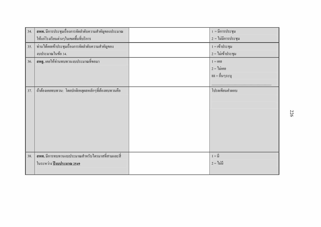
226

34. สพท. มการประชมเรองการจดล าดบความส าคญของประมาณ

ใหแกโรงเรยนตางๆในเขตพนทบรการ 1 = มการประชม

2 = ไมมการประชม

35. ทานไดเคยเขาประชมเรองการจดล าดบความส าคญของงบประมาณในขอ 34.

1 = เขาประชม 2 = ไมเขาประชม

36. สพฐ. เคยใหทานทบทวนงบประมาณทขอมา 1 = เคย 2 = ไมเคย 88 = อนๆระบ __________________________________

37. ถาตองเคยทบทวน: โดยปกตเหตผลหลกๆทตองทบทวนคอ

โปรดเขยนค าตอบ

38. สพท. มการทบทวนงบประมาณส าหรบไตรมาสทสามและส ในระหวาง ปงบประมาณ 2549

1 = ม 2 = ไมม

227

39. ภายหลงการทบทวน สพท. ไดรบ

งบประมาณโดยรวมในปงบประมาณ 2549 เพมขน / ลดลง / ไมเปลยนแปลง

เพมขน

บาท 0 = ไมเปลยนแปลง

ลดลง

ไมเปลยนแปลง

40. สพท. มการทบทวนงบประมาณส าหรบไตรมาสทสามและส ในระหวาง ปงบประมาณ 2550

1 = ใช, 2 = ไมใช

41. ภายหลงการทบทวน สพท. ไดรบ งบประมาณโดยรวมในปงบประมาณ 2550 เพมขน / ลดลง / ไมเปลยนแปลง

เพมขน

บาท 0 = ไมเปลยนแปลง

ลดลง

ไมเปลยนแปลง

228

4. ตนทนทางการศกษาของผปกครอง (เพอเปนขอมลเชงสถตและถาไมมขอมลโปรดท าเครองหมาย —) เงนอดหนนและคาใชจายอนๆทก าหนดโดยส านกงานคณะกรรมการการศกษาขนพนฐาน (สพฐ.) ปงบประมาณ 2549 ปงบประมาณ 2550 ปงบประมาณ 2551 หนวย

เงนอดหนนรายหว คาใชจายอนๆสงสดทเรยกเกบจากผปกครอง*

เงนอดหนนรายหว คาใชจายอนๆ สงสดทเรยกเกบ จากผปกครอง*

เงนอดหนนรายหว คาใชจายอนๆสงสดทเรยกเกบจากผปกครอง*

42. กอนประถม ฯ (อนบาล)

บาท

43. ประถมศกษา

44. มธยมศกษา

* ในกรณไมมคาใชจายอน โปรดท าเครองหมาย —

229

5. งบประมาณโรงเรยนตามรายชอโรงเรยนทผวจยท าการศกษา

ปงบประมาณ 2549 ปงบประมาณ 2550 ปงบประมาณ2551 รหส / หนวย

สนไตรมาส 2 สนไตรมาส 4 สนไตรมาส 2 สนไตรมาส 4 สนไตรมาส 2

45. งบประมาณมาถงโรงเรยนในเขตพนทน

โดยวธใด

1= โอนเขาบญช สพท.

2= โอนเขาบญชโรงเรยน

88= อนๆ ระบ ________

46. จ านวนงบประมาณทโรงเรยนตามรายชอ

ทท าการศกษาไดรบรวมกนทกโรงเรยน

เทากบ*

บาท

47. จ านวนเงนทไดรบเทากบงบประมาณทขอ...

1 = เทากน

2 = ไมเทากน

99 = ไมทราบ

48. ถาไมเทากน: แตกตางกนอยางไร

1 = มากกวาทขอ 2 = นอยกวาทขอ

49. สพท. ไดรบงบประมาณเพอการโอนให โรงเรยนในเดอนใด

1 = ม.ค. 2 = ก.พ. 3 = ม.ค. 4 = เม.ย. 5 = พ.ค. 6 = ม.ย. 7 = ก.ค. 8 = ส.ค. 9 = ก.ย. 10 = ต.ค. 11 = พ.ย. 12 = ธ.ค.

230

ปงบประมาณ 2549 ปงบประมาณ 2550 ปงบประมาณ2551 รหส / หนวย

สนไตรมาส 2 สนไตรมาส 4 สนไตรมาส 2 สนไตรมาส 4 สนไตรมาส 2 50. โดยปกต เงนงบประมาณจะไปถงโรงเรยน

ภายใน…. 1 = หนงอาทตย

2 = สองอาทตย 3 = หนงเดอน 4 = มากกวาหนงเดอน

51. ถาเงนไมไปถงโรงเรยนภายในหนงอาทตย เหตผลส าคญคอ….

1 = เจาหนาทไมเพยงพอ 2 = สวนกลางดง งบประมาณไว 3 = อนๆ ระบ _________

52. โดยปกต โรงเรยนทกแหงไดรบงบประมาณ พรอมกน

1 = พรอม 2 = ไมพรอมกน

53. ถาไมไดรบพรอมกน โดยปกตสดสวนของโรงเรยนทไดรบชากวาโรงเรยนอนๆ

1 = รอยละ 1-5 2 = รอยละ 6-10 3 = รอยละ 11-20 4 = รอยละ 21-40 5 = มากกวารอยละ 40

54. ถางบประมาณของโรงเรยนตองโอนเขาบญช สพท. กอน ในทสดแลวโรงเรยนจะไดรบเงนตามทไดรบอนมต

1 = ได 2 = ไมได 88 = อนๆ ________

231

ปงบประมาณ 2549 ปงบประมาณ 2550 ปงบประมาณ2551 รหส / หนวย

สนไตรมาส 2 สนไตรมาส 4 สนไตรมาส 2 สนไตรมาส 4 สนไตรมาส 2

55. ถาตองโอนเขาบญชของ สพท. กอน โดย

เฉลยแลวมเงนงบประมาณคงคางอยท สพท.

คดเปนรอยละ...

1 = รอยละ 1-5 2 = รอยละ 6-10 3 = รอยละ 11-20 4 = รอยละ 21-40 5 = มากกวารอยละ 40

56. เงนงบประมาณคงคางของโรงเรยนในขอ 53.

สพท. มวธการบรหารคอ...

0 = เกบไวเพอรอการโอน 1 = ใชในงานบรหาร สพท. 2 = ใชในโครงการพเศษ ของ สพท. 88 = อนๆ โปรดระบ _____________

57. ในความคดเหนของทาน เหตผลหลกๆท

โรงเรยนมปญหาในการไดรบงบประมาณ

ตามก าหนดเวลา

โปรดระบเหตผล

58. วธการแกปญหาคอ

โปรดระบวธการ

232

6. จ านวนงบประมาณทงสนตามเอกสาร/รายงานทโอนใหโรงเรยนทท าการศกษา (เพอเปนตวแปรเชงสถต) ขอ ค าถาม ค าตอบ รหส/หนวยค าตอบ

ปงบประมาณ 2549 ปงบประมาณ 2550

59. จ านวนงบประมาณประเภทเงนรายหวทโอนใหโรงเรยนท

ท าการศกษาในปงบประมาณ…

บาท

60. จ านวนงบประมาณประเภทเงนอดหนนทโอนใหโรงเรยนท

ท าการศกษาในปงบประมาณ…

61. จ านวนงบประมาณประเภทเงนรายจายอนทโอนใหโรงเรยนท

ท าการศกษาในปงบประมาณ…

62. ทานสามารถใหส าเนาเอกสาร / รายงานงบประมาณนแกผวจย*

1 = ได 2 = ไมได

233

7. การตรวจสอบภายในของ สพท. (เพอเปนขอมลเชงสถตและเชงคณภาพ) ขอ ค าถาม ค าตอบ รหส/หนวยค าตอบ

63. ส านกงานคณะกรรมการการศกษาขนพนฐานมการตรวจสอบบญชเงนงบประมาณตางๆ

1 = มการตรวจ 2 = ไมมการตรวจ

64. ถามการตรวจ: ก าหนดการตรวจสอบบญช 1 = ทก 3 เดอน 2 = ทก 6 เดอน 3 = ปละครง 88 = อนๆ เชน ___________________

65. จ านวนครงทตรวจในปงบประมาณ 2549 1 = หนงครง 2 = สองครง 3 = สามครง 4 = สครง 5 = มากกวาสครง

66. จ านวนครงทตรวจในปงบประมาณ 2550 1 = หนงครง 2 = สองครง 3 = สามครง 4 = สครง 5 = มากกวาสครง

67. ส านกงานตรวจเงนแผนดนประจ าจงหวดชวย…. 1 = แนะน ากระบวนการงบประมาณ 2 = อธบายเหตผลวาท าไมจงใชงบประมาณไมได 3 = ตรวจสอบการโอนงบประมาณของโรงเรยน 4 = อนๆ ระบ ___________________

234

8. งบประมาณสนบสนนส าหรบโรงเรยนจากหนวยงานรฐอนๆ ในปงบประมาณ 2550

หนวยงานทสนบสนน งบประมาณทขอ งบประมาณทได โปรดระบโครงการทจะน าไปใช

68. องคการบรหารสวนจงหวด

69. องคการบรหารสวนต าบล

70. เทศบาล

71. หนวยงานราชการอนๆในพนท (ระบชอหนวยงาน)

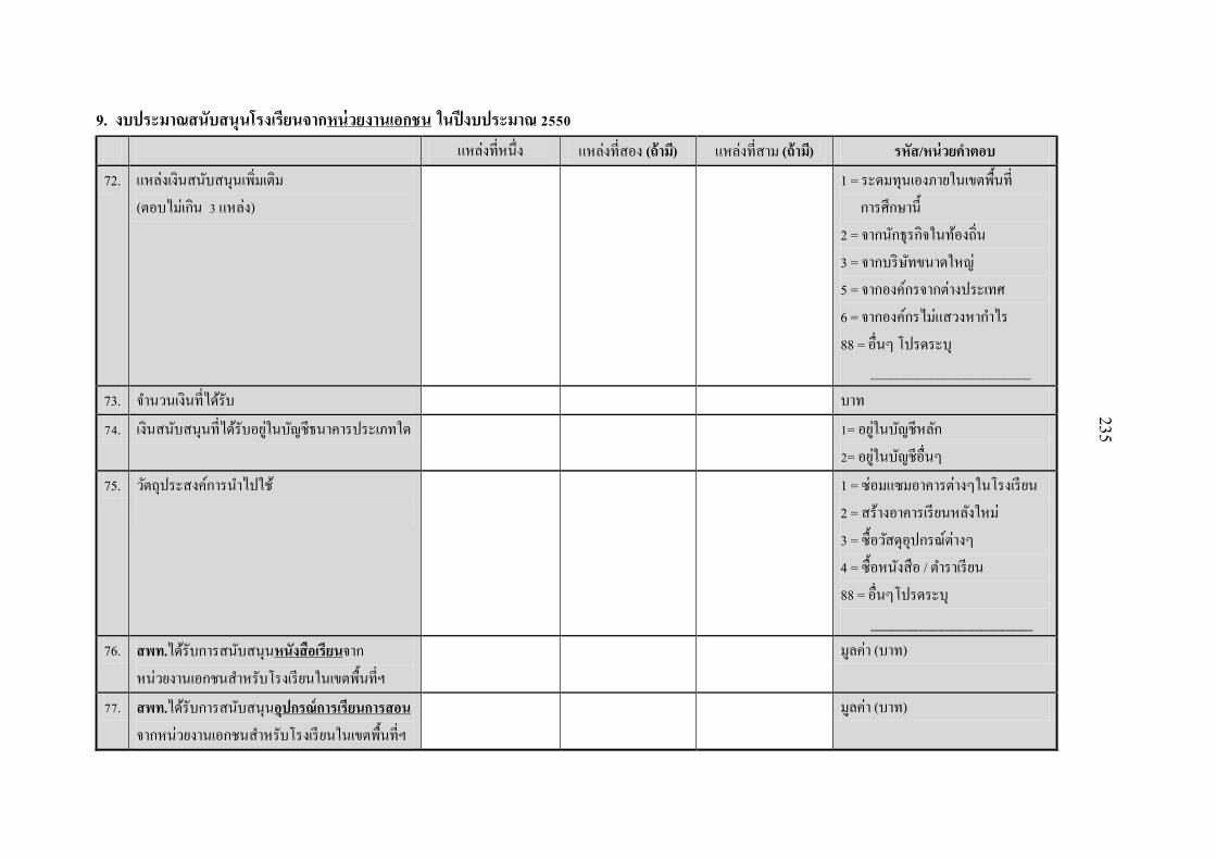
235

9. งบประมาณสนบสนนโรงเรยนจากหนวยงานเอกชน ในปงบประมาณ 2550

แหลงทหนง แหลงทสอง (ถาม) แหลงทสาม (ถาม) รหส/หนวยค าตอบ

72. แหลงเงนสนบสนนเพมเตม (ตอบไมเกน 3 แหลง)

1 = ระดมทนเองภายในเขตพนท การศกษาน 2 = จากนกธรกจในทองถน 3 = จากบรษทขนาดใหญ 5 = จากองคกรจากตางประเทศ 6 = จากองคกรไมแสวงหาก าไร 88 = อนๆ โปรดระบ ________________________

73. จ านวนเงนทไดรบ บาท 74. เงนสนบสนนทไดรบอยในบญชธนาคารประเภทใด 1= อยในบญชหลก

2= อยในบญชอนๆ 75. วตถประสงคการน าไปใช

1 = ซอมแซมอาคารตางๆในโรงเรยน

2 = สรางอาคารเรยนหลงใหม 3 = ซอวสดอปกรณตางๆ 4 = ซอหนงสอ / ต าราเรยน

88 = อนๆโปรดระบ ________________

76. สพท.ไดรบการสนบสนนหนงสอเรยนจากหนวยงานเอกชนส าหรบโรงเรยนในเขตพนทฯ

มลคา (บาท)

77. สพท.ไดรบการสนบสนนอปกรณการเรยนการสอนจากหนวยงานเอกชนส าหรบโรงเรยนในเขตพนทฯ

มลคา (บาท)

236

78. ถาเปนบญชหลก เปนบญชของหนวยงานใด (ถาเปนบญชอนๆ ขามไปท าขอตอไป)

1 = ของโรงเรยน

3 = ของส านกงานเขตพนทการศกษา (สพท.) 4 = ของคณะกรรมการสถานศกษาขน พนฐาน 88 = อนๆ ระบ _________________

79. ถาเปนบญชอนๆ เปนบญชของหนวยงานใด

1 = ของโรงเรยน

3 = ของส านกงานเขตพนทการศกษา (สพท.) 4 = ของคณะกรรมการสถานศกษาขน พนฐาน 88 = อนๆ ระบ__________________

80. เงนสนบสนนทไดรบอยในบญชธนาคารอนๆ ของหนวยงานใด…

1 = บญชของส านกงานเขตพนท การศกษา 2 = บญชของโรงเรยน

3 = คณะกรรมการสถานศกษาขน พนฐาน 88 = อนๆ ระบ __________________

237

81. ผทไดรบมอบอ านาจใหเบกจายเงนสนบสนนได

1 = ส านกงานเขตพนทการศกษา

2 = ผบรจาคด าเนนการเอง

3 = โรงเรยน

4 = คณะกรรมการสถานศกษาขนพนฐาน 88 = อนๆ ระบ

_____________________________

238

10. บทบาทในการจดการศกษาในโรงเรยนในเขตพนทฯ (เพอเปนตวแปรเชงสถต) ขอ ค าถาม ค าตอบ

ในความคดเหนของทาน ผทพจารณาในเรองดงตอไปนของ

โรงเรยนคอ….

ก ข ค

ผพจารณาหลก… ผมสวนรวมพจารณา… ทานมสวนรวมพจารณา

1 = ส านกงานคณะกรรมการฯ (สพฐ.) 2 = ส านกงานเขตพนทฯ (สพท.) 3 = คณะกรรมการสถานศกษา 4 = ผตรวจ 5 = ผอ านวยการ 6 = ผน าการเมองทองถน 7 = ผบรจาคเงนใหโรงเรยน 8 = องคกรไมแสวงหาก าไรท สนบสนนโรงเรยน 9 = สมาคมครและผปกครอง 10 = คณะกรรมการ ก.ค.ศ. 11 = คณะกรรมการ อ.ก.ค.ศ. 12 = องคกรธรกจทสนบสนน ร.ร. 88 = อนๆ ___________________

1 = ส านกงานคณะกรรมการฯ สพฐ.) 2 = ส านกงานเขตพนทฯ (สพท.) 3 = คณะกรรมการสถานศกษา 4 = ผตรวจ 5 = ผอ านวยการ 6 = ผน าการเมองทองถน 7 = ผบรจาคเงนใหโรงเรยน 8 = องคกรไมแสวงหาก าไรท สนบสนนโรงเรยน 9 = สมาคมครและผปกครอง 10 = คณะกรรมการ ก.ค.ศ. 11 = คณะกรรมการ อ.ก.ค.ศ. 12 = องคกรธรกจทสนบสนน ร.ร. 88 = อนๆ ___________________

1 = ไมม

2 = มบาง

3 = มมาก

1. วธการสอนในโรงเรยน

2. การรบเดกนกเรยนเขาเรยน

3. การก าหนดจ านวนนกเรยนตอหอง

239

ในความคดเหนของทาน ผทพจารณาในเรองดงตอไปนคอ….(ตอ) ผพจารณาหลก… ผมสวนรวมพจารณา… ทานมสวนรวมพจารณา

4. การประเมนผลการเรยนของนกเรยน

5. การก าหนดนโยบายประเมนผลการเรยนของนกเรยน

6. การบรรจครมาท างานในโรงเรยน

7. การประเมนการท างานของครใน ร.ร.

8. การก าหนดนโยบายประเมนผลการสอนของคร

9. การเลอนขนใหคร

10. การลงโทษทางวนย

11. การสงครไปอบรม

12. การก าหนดจ านวนเงนคากจกรรม

13. การใชเงนคากจกรรม

14. การใชเงนอดหนนโรงเรยน

15. การจางเหมาซอมแซมโรงเรยน

16. การสรางหองเรยนใหม

17. การจดการประชมครและผปกครอง

18. การจดกจกรรมกบชมชน

19. การระดมทนของโรงเรยน

240

11. ขอด/โอกาสและสงทตองปรบปรง / อปสรรค ขอด / โอกาส และสงทตองปรบปรง / อปสรรคสามขอหลก... ขอด / โอกาส สงทตองปรบปรง / อปสรรค

1. ภาพรวมของการบรการการศกษาในเขตพนทการศกษาน 1.

1.

2.

2.

3.

3.

241

2. ภาพรวมของการเรยนของเดกนกเรยนในระดบโรงเรยน

ในเขตพนทการศกษาน

1.

1.

2.

2.

3.

3.

242

แบบสอบถามเลขานการคณะกรรมการสถานศกษาขนพนฐาน

243

แบบสอบถามส าหรบวทยานพนธปรญญาเอกสาขาเศรษฐศาสตรเรอง

“School Expenditure Leakage and Efficiency: The Case of Thai Compulsory Education”

ค าชแจง 1. โปรดตอบค าถามโดยลงรหสค าตอบ/ค าตอบลงในชองวางโดยใชปากกา ดงตวอยาง ขอ ค าถาม ค าตอบ รหส / หนวยค าตอบ

11 ทานเกดในจงหวดน 1 1 = ใช 2 = ไมใช 12 วฒการศกษาสงสดของทาน 5

1 = ไมเปนทางการ 2 = ประถมศกษา 3 = มธยมศกษาตอนตน 4 = มธยมศกษาตอนปลาย 5 = ปรญญาตร 6 = สงกวาปรญญาตร

2. ในขอทไมมรหสค าตอบ โปรดเตมค าตอบในชองวางหรอเนอทวาง 3. โปรดเตมค าตอบทกขอโดยเฉพาะสวนทเกยวกบบรหารการเงนของโรงเรยนเพอทจะสามารถน าขอมลไปค านวณทางสถต และแปลผลตามหลกวชาการ 4. โปรดท าเครองหมาย — ในชองทไมมขอมล 5. ขอมลทงหมดเปนความลบและใชเพอการศกษาวจยเทานน 6. วทยานพนธนสวนหนงจะลงพมพในวารสารวชาการ (ตามขอก าหนดของส านกงานคณะกรรมการการอดมศกษา) 7. ผวจยขอขอบคณทกทานอยางสงทอนเคราะหขอมลเพอเปนประโยชนในทางวชาการ

8. ผวจยจะเดนทางเขาไปรบแบบสอบถามในชวงเวลา 2- 4 สปดาหภายหลงจากไดรบแบบสอบถาม ชอผวจย นายจระเดช ทศยาพนธ นกศกษาปรญญาเอกคณะพฒนาการเศรษฐกจ สถาบนบณฑตพฒนบรหารศาสตร (นดา)

โทร. 081 1700051 emails: jiradate.t@hotmail.com, jiradate.t@gmail.com

244

ชดแบบสอบถามเลขานการคณะกรรมการสถานศกษาขนพนฐาน

1. ขอมลพนฐาน แบบสอบถามชดท ______________________ รหสโรงเรยน __________________________ ขอ ค าถาม ค าตอบ รหส / หนวยค าตอบ

1. ชอโรงเรยน ชอ 2. ทอยโรงเรยน

หมบาน / ต าบล / อ าเภอ / จงหวด

3. วน/เดอน/ปทตอบแบบสอบถาม / / 2551 วน / เดอน / ป

4. ชอผตอบแบบสอบถาม ชอ 5. เพศ 1 = ชาย 2 = หญง 6. อาย ป 7. สถานภาพ 1 = โสด 2 = สมรส 3 = หยาราง 8. ทานเปนเลขานการคณะกรรมการสถานศกษาขนพนฐาน 1 = เปน 2 = ไมไดเปน 9. ถาไมใช : โปรดระบต าแหนงหนาทในคณะกรรมการฯน ระบต าแหนง 10. ทานเกดในอ าเภอน 1 = ใช 2 = ไมใช 11. ทานเกดในจงหวดน 12. วฒการศกษาสงสดของทาน 1 = ไมไดเขาศกษาในระบบโรงเรยน

2 = ประถมศกษา 3 = มธยมศกษาตอนตน 4 = มธยมศกษาตอนปลาย 5 = ปรญญาตร 6 = สงกวาปรญญาตร

245

2. การบรหารการเงนของสถานศกษา ขอ ค าถาม ค าตอบ รหส / หนวยค าตอบ

โปรดตอบแบบสอบถามในสวนทโรงเรยนมบญชธนาคารตอไปนทกบญช 1. มบญชธนาคารหลกรวมกนระหวางโรงเรยนและ

คณะกรรมการสถานศกษาขนพนฐาน 1 = ม

2 =ไม ม 88 = อนๆ ระบ _________________

2. ถามบญชธนาคารตาม ขอ 1. ระบจ านวนบญชทงหมดทม จ านวนบญช

3. มบญชธนาคารหลกของโรงเรยน

1 = ม 2 =ไม ม 88 = อนๆ ระบ _________________

4. ถามบญชธนาคารตาม ขอ 3. ระบจ านวนบญชทงหมดทม จ านวนบญช

5. มบญชธนาคารหลกของคณะกรรมการสถานศกษาขนพนฐาน 1 = ม 2 =ไม ม 88 = อนๆ ระบ _________________

6. ถามบญชธนาคารตาม ขอ 5. ระบจ านวนบญชทงหมดทม จ านวนบญช

7. มบญชธนาคารอนๆของโรงเรยน (รวมทง เปดบญชเพอรบเงนบรจาค เปนตน)

1 = ม 2 =ไม ม 88 = อนๆ ระบ _________________

8. ถามบญชธนาคารตาม ขอ 7. ระบจ านวนบญชทงหมดทม จ านวนบญช

246

กรณมการใชบญชธนาคารหลกรวมกนระหวางโรงเรยนและคณะกรรมการสถานศกษาขนพนฐาน (เพอทราบแนวทางการบรหารการเงน)

ขอ ค าถาม ค าตอบ หนวย 9. จ านวนเงนทงหมดทเบกออกจากบญชธนาคารหลกรวมกน

ระหวางโรงเรยนและคณะกรรมการสถานศกษาขนพนฐาน เพองานดงตอไปนในปงบประมาณ...

บญชหลก บาท

ปงบประมาณ 2549 ปงบประมาณ 2550

9ก. การซอมแซมทวๆไป 9ข. การสรางอาคารสถานทตางๆ 9ค. ครภณฑพนฐานตางๆ 9ง. หนงสอและต าราเรยน 9จ. วสดสนเปลองตางๆ 9ฉ. อปกรณการเรยนการสอน 9ช. การเดนทางและการขนสง 9ซ. จางคนท างานพเศษ 9ฌ. ครจางสอน 9ญ. อนๆ เชน _______________________________________

_________________________

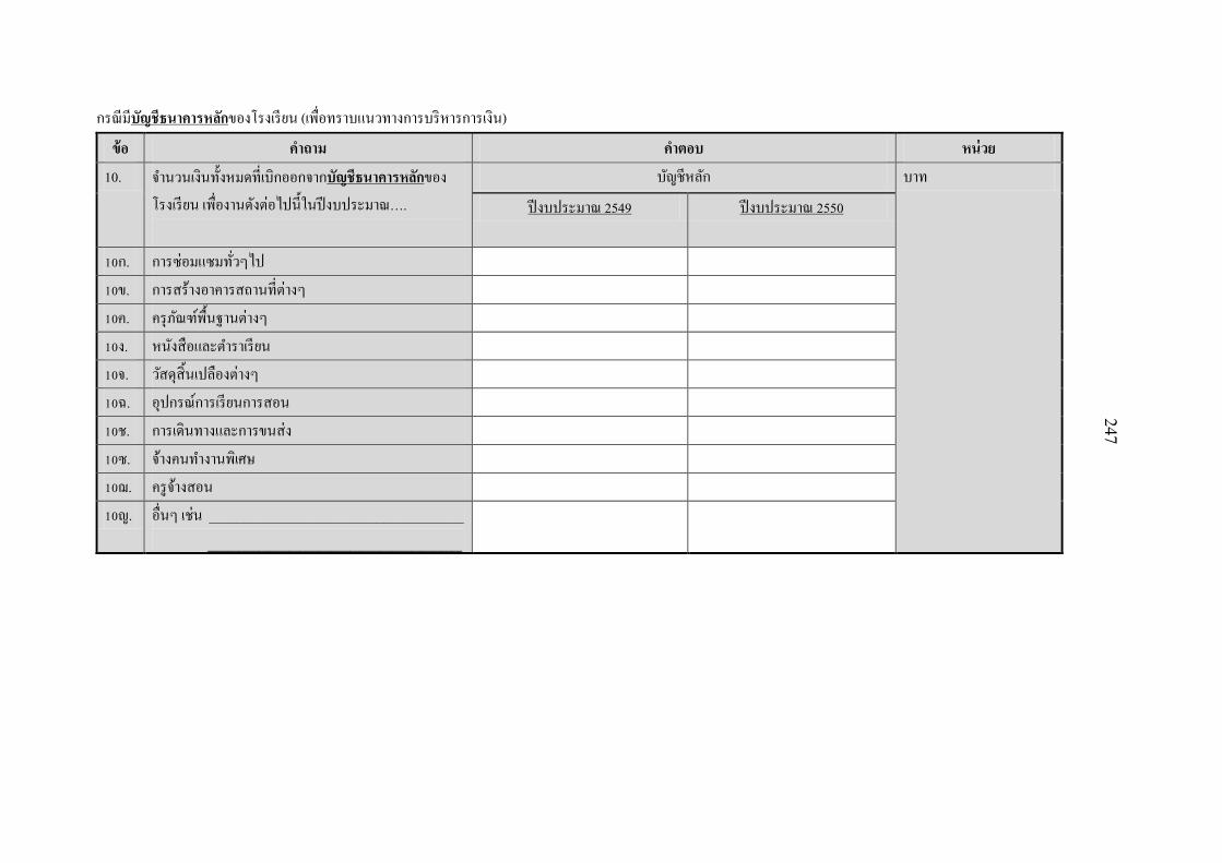
247

กรณมบญชธนาคารหลกของโรงเรยน (เพอทราบแนวทางการบรหารการเงน)

ขอ ค าถาม ค าตอบ หนวย 10. จ านวนเงนทงหมดทเบกออกจากบญชธนาคารหลกของ

โรงเรยน เพองานดงตอไปนในปงบประมาณ….

บญชหลก บาท

ปงบประมาณ 2549 ปงบประมาณ 2550

10ก. การซอมแซมทวๆไป 10ข. การสรางอาคารสถานทตางๆ 10ค. ครภณฑพนฐานตางๆ 10ง. หนงสอและต าราเรยน 10จ. วสดสนเปลองตางๆ 10ฉ. อปกรณการเรยนการสอน 10ช. การเดนทางและการขนสง 10ซ. จางคนท างานพเศษ 10ฌ. ครจางสอน 10ญ. อนๆ เชน ______________________________________

_________________________

248

กรณมการใชบญชธนาคารหลกของคณะกรรมการสถานศกษาขนพนฐาน (เพอทราบแนวทางการบรหารการเงน)

ขอ ค าถาม ค าตอบ หนวย 11. จ านวนเงนทงหมดทเบกออกจากบญชธนาคารหลกของ

คณะกรรมการสถานศกษาขนพนฐาน เพองานดงตอไปนในปงบประมาณ….

บญชหลก บาท

ปงบประมาณ 2549 ปงบประมาณ 2550

11ก. การซอมแซมทวๆไป 11ข. การสรางอาคารสถานทตางๆ 11ค. ครภณฑพนฐานตางๆ 11ง. หนงสอและต าราเรยน 11จ. วสดสนเปลองตางๆ 11ฉ. อปกรณการเรยนการสอน 11ช. การเดนทางและการขนสง 11ซ. จางคนท างานพเศษ 11ฌ. ครจางสอน 11ญ. อนๆ เชน _____________________________________

________________________

249

กรณมการใชมบญชธนาคารอนๆ เพองานของโรงเรยน ระบชอบญช ___________________________ (เพอทราบแนวทางการบรหารการเงน)

ขอ ค าถาม ค าตอบ หนวย 12. จ านวนเงนทงหมดทเบกออกจากบญชธนาคารอนๆ เพอ

งานของโรงเรยนดงตอไปนในปงบประมาณ….

บญชอนๆ (ถาม) บาท

ปงบประมาณ 2549 ปงบประมาณ 2550

12ก. การซอมแซมทวๆไป 12ข. การสรางอาคารสถานทตางๆ 12ค. ครภณฑพนฐานตางๆ 12ง. หนงสอและต าราเรยน 12จ. วสดสนเปลองตางๆ 12ฉ. อปกรณการเรยนการสอน 12ช. การเดนทางและการขนสง 12ซ. จางคนท างานพเศษ 12ฌ. ครจางสอน 12ญ. อนๆ เชน ____________________________________

________________________

250

3. บทบาทและความรบผดชอบในการบรหารการศกษาในสถานศกษา (เพอเปนตวแปรเชงสถต) ขอ ค าถาม ค าตอบ

ในความคดเหนของทาน ผทพจารณาในเรองดงตอไปน

ของโรงเรยนคอ….

ก ข ค

ผพจารณาหลก… ผมสวนรวมพจารณา… ทานมสวนรวมพจารณา

1 = ส านกงานคณะกรรมการฯ (สพฐ.) 2 = ส านกงานเขตพนทฯ (สพท.) 3 = คณะกรรมการสถานศกษา 4 = ผตรวจ 5 = ผอ านวยการ 6 = ผน าการเมองทองถน 7 = ผบรจาคเงนใหโรงเรยน 8 = องคกรไมแสวงหาก าไรท สนบสนนโรงเรยน 9 = สมาคมครและผปกครอง 10 = คณะกรรมการ ก.ค.ศ. 11 = คณะกรรมการ อ.ก.ค.ศ. 12 = องคกรธรกจทสนบสนน ร.ร. 88 = อนๆ ___________________

1 = ส านกงานคณะกรรมการฯ สพฐ.) 2 = ส านกงานเขตพนทฯ (สพท.) 3 = คณะกรรมการสถานศกษา 4 = ผตรวจ 5 = ผอ านวยการ 6 = ผน าการเมองทองถน 7 = ผบรจาคเงนใหโรงเรยน 8 = องคกรไมแสวงหาก าไรท สนบสนนโรงเรยน 9 = สมาคมครและผปกครอง 10 = คณะกรรมการ ก.ค.ศ. 11 = คณะกรรมการ อ.ก.ค.ศ. 12 = องคกรธรกจทสนบสนน ร.ร. 88 = อนๆ ___________________

1 = ไมม

2 = มบาง

3 = มมาก

1. วธการสอนในโรงเรยน

2. การรบเดกนกเรยนเขาเรยน

3. การก าหนดจ านวนนกเรยนตอหอง

251

ในความคดเหนของทาน ผทพจารณาในเรองดงตอไปนคอ….(ตอ) ผพจารณาหลก… ผมสวนรวมพจารณา… ทานมสวนรวมพจารณา

4. การประเมนผลการเรยนของนกเรยน

5. การก าหนดนโยบายประเมนผลการเรยนของนกเรยน

6. การบรรจครมาท างานในโรงเรยน

7. การประเมนการท างานของครใน ร.ร.

8. การก าหนดนโยบายประเมนผลการสอนของคร

9. การเลอนขนใหคร

10. การลงโทษทางวนย

11. การสงครไปอบรม

12. การก าหนดจ านวนเงนคากจกรรม

13. การใชเงนคากจกรรม

14. การใชเงนอดหนนโรงเรยน

15. การจางเหมาซอมแซมโรงเรยน

16. การสรางหองเรยนใหม

17. การจดการประชมครและผปกครอง

18. การจดกจกรรมกบชมชน

19. การระดมทนของโรงเรยน

252

แบบสอบถามผปกครองนกเรยนทจบการศกษาชน ม.3 ในปการศกษา 2550

253

แบบสอบถามส าหรบวทยานพนธปรญญาเอกสาขาเศรษฐศาสตรเรอง

“School Expenditure Leakage and Efficiency: The Case of Thai Compulsory Education”

ค าชแจง 1. โปรดตอบค าถามโดยลงรหสค าตอบ/ค าตอบ ลงในชองวางโดยใชปากกา ดงตวอยาง ขอ ค าถาม ค าตอบ รหส / หนวยค าตอบ

5 ทานเปนศษยเกาโรงเรยนน 1 1 = ใช 2 = ไมใช 6 วฒการศกษาสงสด 4

1 = ไมเคยเขาศกษาในโรงเรยน

2 = ประถมศกษา 3 = มธยมศกษาตอนตน 4 = มธยมศกษาตอนปลาย 5 = ปรญญาตร 6 = สงกวาปรญญาตร

2. ในขอทไมมรหสค าตอบ โปรดเตมค าตอบในชองวางหรอเนอทวาง 3. โปรดเตมค าตอบทกขอโดยเฉพาะความคดเหนตอโรงเรยนเพอทจะสามารถน าขอมลไปค านวณทางสถตและแปลผลตามหลกวชาการ 4. โปรดท าเครองหมาย — ในชองทไมมขอมล 5. ขอมลทงหมดเปนความลบและใชเพอการศกษาวจยเทานน 6. วทยานพนธนสวนหนงจะลงพมพในวารสารวชาการ (ตามขอก าหนดของส านกงานคณะกรรมการการอดมศกษา) 7. ผวจยขอขอบคณทกทานอยางสงทอนเคราะหขอมลเพอเปนประโยชนในทางวชาการ 8. ผวจยจะเดนทางเขาไปรบแบบสอบถามในชวงเวลา 2- 4 สปดาหภายหลงจากไดรบแบบสอบถาม

ชอผวจย นายจระเดช ทศยาพนธ นกศกษาปรญญาเอกคณะพฒนาการเศรษฐกจ สถาบนบณฑตพฒนบรหารศาสตร (นดา) โทร. 081 1700051 emails: jiradate.t@hotmail.com, jiradate.t@gmail.com

254

ชดแบบสอบถามผปกครองนกเรยน

1. ขอมลทวไป แบบสอบถามชดท _______________รหสโรงเรยน ________________________ ขอ ค าถาม ค าตอบ รหส / หนวยค าตอบ 1. ชอบตรทจบชนมธยมศกษาปท 3 ในปทผานมา ชอนกเรยน 2. ชอผปกครอง ชอผปกครอง 3. ทอยของทาน

หมบาน / ต าบล / อ าเภอ / จงหวด

4. วน/เดอน/ปทตอบแบบสอบถาม / / 2551 วน / เดอน / ป 5. เพศ 1 = ชาย 2 = หญง 6. สถานภาพ 1 = สมรส 2= หยาราง 7. ทานเปนศษยเกาโรงเรยนน 1 = ใช 2 = ไมใช 8. วฒการศกษาสงสด 1 = ไมไดเขาศกษาในระบบโรงเรยน

2 = ประถมศกษา 3 = มธยมศกษาตอนตน 4 = มธยมศกษาตอนปลาย 5 = ปรญญาตร 6 = สงกวาปรญญาตร

9. จ านวนบตร ระบจ านวน 10. รายไดรวมเฉลยทงครวเรอนตอเดอน บาท

11. มโรงเรยนอนใกลเคยงททานสามารถใหบตรไปเขาเรยนแทน.. 1 = ม 2 = ไมม 99 = ไมทราบ

255

12. ถาม: เหตใดทานจงใหบตรเรยนทโรงเรยนน

โปรดเขยนเหตผล

13. ทานเขาไปเยยมโรงเรยนมากนอยเพยงใด

(ถาไมเคยเขาไปเยยมโรงเรยน ขามไปขอ 14.)

1 = บอยๆ 2 = บางครง

3 = นานๆครง 4 = ไมเคย

14. เหตผลททานเขาไปเยยมโรงเรยน

โปรดเขยนเหตผล

15. ทานคดวาบตรของทานชอบโรงเรยนนหรอไม 1 = ชอบ 2 = ไมชอบ

3 = ไมมความเหน 99 = ไมทราบ

16. จากขอ 14 บตรของทานพดถงโรงเรยนวาอยางไร

โปรดเขยนค าตอบ

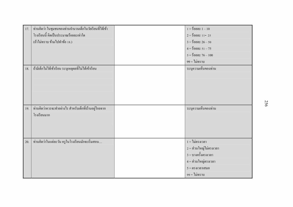
256

17. ทานคดวา ในชมชนของทานจ านวนเดกในวยเรยนทไดเขา

โรงเรยนน คดเปนประมาณรอยละเทาใด (ถาไมทราบ ขามไปท าขอ 18.)

1 = รอยละ 1 – 10 2 = รอยละ 11- 25 3 = รอยละ 26 – 50 4 = รอยละ 51 – 75 5 = รอยละ 76 – 100 99 = ไมทราบ

18. ถามเดกไมไดเขาเรยน ระบเหตผลทไมไดเขาเรยน

ระบความเหนของทาน

19. ทานคดวาควรจะท าอยางไร ส าหรบเดกทบานอยไกลจาก โรงเรยนมาก

ระบความเหนของทาน

20. ทานคดวาในแตละวน ครในโรงเรยนมกจะเรมสอน… 1 = ไมตรงเวลา 2 = สวนใหญไมตรงเวลา 3 = บางครงตรงเวลา 4 = สวนใหญตรงเวลา 5 = ตรงเวลาเสมอ 99 = ไมทราบ

257

21. ครในโรงเรยนใชเวลาการสอนหนงสอทโรงเรยน

1 = ไมอยสอนเลย

2 = ไมสอนเปนสวนใหญ 3 = ไมสอนเปนบางครง 4 = สวนใหญสอน 5 = สอนอยทโรงเรยนเสมอ 99 = ไมทราบ

22. ผอ. / รอง ผอ. โรงเรยนไดเขามาเยยมและพบปะกบผปกครอง 1 = ไมมาเยยมเลย 2 = ไมมาเปนสวนใหญ 3 = มาเปนบางครง 4 = สวนใหญมา 5 = มาเยยมอยเสมอ

23. ครในโรงเรยนไดเขามาเยยมพบปะกบผปกครอง 1 = ไมมาเยยมเลย 2 = ไมมาเปนสวนใหญ 3 = มาเปนบางครง 4 = สวนใหญมา 5 = มาเยยมอยเสมอ

24. ทานคดวาคณะกรรมการสถานศกษาขนพนฐานมหนาท….

โปรดเขยนค าตอบ

25. ทานคดวาคณะกรรมการสถานศกษาขนพนฐานท างานไดด 1 = ด

2 = ไมด 99 = ไมทราบ

258

26. ทานคดวาโรงเรยนนประสบปญหาหลกๆใดบางในขณะน

(ตอบไมเกน 4 ค าตอบ) 1.

2. 3. 4.

27. ทานคดวาใครควรจะเปนผรบภาระคาใชจายทางการศกษา

1 = รฐ 2 = ผปกครองนกเรยน 3 = รฐและผปกครองนกเรยนชวยกน 88 = อนๆ โปรดระบ ____________________

28. โรงเรยนมการเกบคาเทอมหรอไม

(ถาไมเกบคาเทอมขามไปท าขอ 34.) 1 = เกบ

2 = ไมเกบ

29. ในปงบประมาณ 2550 ทานสามารถจายคาเทอมของบตรได 1 = ช าระไดทงหมด 2 = ช าระไดบางสวน 3 = ช าระไมไดเลย

30. ในปงบประมาณ 2550 ทานมสวนรวมกบโรงเรยนในก าหนดคาเทอม

1 = มสวนรวม 2 = ไมมสวนรวม

259

31. ถามสวนรวม ทานมสวนรวมอยางไร

ระบการมสวนรวมของทาน

32. ทานคดวาจ านวนคาเทอมทโรงเรยนเรยกเกบเปนอยางไร

1 = ต าเกนไป 2 = เหมาะสม 3 = สงเกนไป 99 = ไมทราบ

33. ในกรณทไมสามารถจายคาเทอมได ทานคดวาควรมมาตรการใดทเหมาะสมเพอใหเดกไดเขาโรงเรยน

ระบมาตรการ

34. หากผปกครองไมสามารถจายคาเทอมได ใครควรเปนผใหความชวยเหลอ

1 = รฐ 2 = โรงเรยน 3 = ชมชน 4 = ญาตพนองของครอบครว 88 = อนๆ ระบ _______________

35. โรงเรยนมการเกบคาใชจายอนๆในการเรยนหรอไม (ถาไมเกบคาใชจายอน ขามไปท าขอ 41.)

1 = เกบ 2 = ไมเกบ

36. ในปงบประมาณ 2550 ทานสามารถจายคาใชจายอนๆนอกเหนอจากคาเทอมในการเรยนของบตรได

1 = ช าระไดทงหมด 2 = ช าระไดบางสวน 3 = ช าระไมไดเลย

37. ทานมสวนรวมกบโรงเรยนในการตดสนใจก าหนด คาใชจายอนๆในการเรยน

1 = มสวนรวม 2 = ไมมสวนรวม

260

38. ถามสวนรวม ทานมสวนรวมอยางไร

ระบการมสวนรวมของทาน

39. ทานคดวาจ านวนคาใชจายอนๆทโรงเรยนเรยกเกบในปการศกษาทผานมา เปนอยางไร

1 = ต าเกนไป 2 = เหมาะสม 3 = สงเกนไป 99 = ไมทราบ

40. ในกรณทไมสามารถจายคาใชจายอนๆ ได ทานคดวาควรมมาตรการใดทเหมาะสมเพอใหเดกไดเขาโรงเรยน

ระบมาตรการ

41. หากผปกครองไมสามารถจายคาใชจายอนๆได ใครควรเปน

ผใหความชวยเหลอ 1 = รฐ 2 = โรงเรยน

3 = ชมชน 4 = ญาตพนองของครอบครว 88 = อนๆ ระบ _______________

42. ความคดเหนเกยวกบคณภาพการเรยนการสอนของโรงเรยน

1 = ด 2 = พอใช 3 = ไมด 88 = อนๆ ระบ _______________

43. บตรของทานไดรบการศกษาตามทคาดหวงหรอไม 1 = ใช 2 = ไมใช 99 = ไมทราบ 44. ในปการศกษา 2549 (ปทผานมา) สมาชกสภาผแทนราษฎร

(ส.ส.) ในเขตเลอกตงนไดชวยเหลอโรงเรยนน 1 = ใช

2 = ไมใช 99 = ไมทราบ

261

45. ถาไดชวยเหลอ : ส.ส. ทานนชวยเหลอในดานใด 1 = การกอสรางอาคารใหม

2 = จดหาอปกรณตางๆใหโรงเรยน 3 = ใหทนเปนคาเลาเรยน 88 = อนๆโปรดระบ ___________________

46. ในปการศกษา 2550 (ปปจจบน) ส.ส. ในเขตนไดชวยเหลอโรงเรยนน.

1 = ใช 2 = ไมใช 99 = ไมทราบ

47. ถาไดชวยเหลอ : ส.ส. ทานนชวยเหลอในดานใด 1 = การกอสรางอาคารใหม 2 = จดหาอปกรณตางๆใหโรงเรยน 3 = ใหทนเปนคาเลาเรยน 88 = อนๆโปรดระบ _____________________

2. บทบาทของทานตอโรงเรยน (เพอใชเปนขอมลเชงสถต) ขอ ค าถาม ค าตอบ รหส / หนวยค าตอบ 1. มสมาคมครและผปกครองในโรงเรยนน

(ถาไมม ขามไปท าขอ 6.) 1 = ม

2 = ไมม

2. มการประชมสมาคมทงหมดกครงใน ปงบประมาณ 2549 จ านวนครง 3. มการประชมสมาคมทงหมดกครงใน ปงบประมาณ 2550

จ านวนครง

4. มการประชมสมาคมทงหมดกครงใน ปงบประมาณ 2551 (นบถงวนทตอบแบบสอบถาม)

จ านวนครง

5. วนทมการประชมสมาคมครงลาสด / / 2551 วน / เดอน / ป

262

6. มผปกครองไดเขามาอานรายงานการตรวจเยยมโรงเรยนของ ส านกงานเขตพนทการศกษา (สพท.) (ถาไมม ขามไปท าขอ 8.)

1 = อาน 2 = ไมอาน

7. ถาม : รอยละของจ านวนผปกครองทไดเขามาอานรายงาน

1 = รอยละ 1 – 10 2 = รอยละ 11- 25 3 = รอยละ 26 – 50 4 = รอยละ 51 – 75 5 = รอยละ 76 – 100 99 = ไมทราบ

8. โรงเรยนเคยเรยกประชมกบผปกครองเพอแกปญหาบางอยางของโรงเรยน (ถาไมม ขามไปท าขอ 10.)

1 = เคยเรยก 2 = ไมเคยเรยก

9. ถาเคยเรยก : จ านวนรอยละของผทเขารวมประชม 1 = รอยละ 1 – 10 2 = รอยละ 11- 25 3 = รอยละ 26 – 50 4 = รอยละ 51 – 75 5 = รอยละ 76 – 100

99 = ไมทราบ

10. ครเคยมการจดกจกรรมรวมกบชมชนเชน การแขงขนกฬา 1 = เคย 2 = ไมเคย 99 = ไมทราบ

11. สมาชกในชมชนไดเคยเขามารวมสอนในโรงเรยน

263

12. ชมชนใหโรงเรยนใชทดนในการเรยนการสอน

วชาเกษตรกรรม

1 = ใหใช 2 = ไมใหใช 88 = อนๆระบ ____________ 99 = ไมทราบ

13. ชมชนเคยใชสถานทของโรงเรยนในงานดงน 1 = เคย 2 = ไมเคย 99 = ไมทราบ

13ก. …การประชม

13ข. …การศกษาอบรมของชมชน

13ค. …งานกฬาของชมชน

3. ผลสมฤทธทางการศกษาบตรของทาน วชา คะแนนการสอบวดผลสมฤทธทางการศกษา ป 2550 (National Test)

1 คณตศาสตร

2 วทยาศาสตร

3 ภาษาองกฤษ

4 ภาษาไทย

5 สงคมศกษา ศาสนา และวฒนธรรม

264

4. ขอดและสงทควรปรบปรงของโรงเรยนน แบบสอบถามชดท __________________________รหสโรงเรยน _______________________

ขอดของโรงเรยนน สงทควรปรบปรงในโรงเรยนน ผปกครองคนอนๆททานรจกคดเหนอยางไรตอโรงเรยนน

1.

2.

3.

BIOGRAPHY

NAME Jiradate Thasayaphan

ACADEMIC BACKGROUND Bachelor’s Degree with a major in

Pharmaceutical Science from Prince

of Songkla University, Songkla

Province, Thailand in 1991. Master’s

Degree in Computer and Engineering

Management at Assumption

University, Bangkok, Thailand in

1997 and Master of Business

Administration at Kasetsart

University, Bangkok, Thailand in

2004.