LUND UNIVERSITY

PO Box 117221 00 Lund+46 46-222 00 00

Scattering from frequency selective surfaces: An efficient set of V-dipole basisfunctions

Poulsen, Sören

Published: 2000-01-01

Link to publication

Citation for published version (APA):Poulsen, S. (2000). Scattering from frequency selective surfaces: An efficient set of V-dipole basis functions.(Technical Report LUTEDX/(TEAT-7083)/1-17/(2000); Vol. TEAT-7083). [Publisher information missing].

General rightsCopyright and moral rights for the publications made accessible in the public portal are retained by the authorsand/or other copyright owners and it is a condition of accessing publications that users recognise and abide by thelegal requirements associated with these rights.

• Users may download and print one copy of any publication from the public portal for the purpose of privatestudy or research. • You may not further distribute the material or use it for any profit-making activity or commercial gain • You may freely distribute the URL identifying the publication in the public portal

CODEN:LUTEDX/(TEAT-7083)/1-20/(2000)

Revision No. 1: February 2002

Scattering from frequency selectivesurfaces: An efficient set of V-dipolebasis functions

Sören Poulsen

Department of ElectroscienceElectromagnetic TheoryLund Institute of TechnologySweden

Soren PoulsenEmail: Soren.Poulsen@acab.se

Applied Composites ABP.O. Box 163SE-341 23 LjungbySweden

and

Department of ElectroscienceElectromagnetic TheoryLund Institute of TechnologyP.O. Box 118SE-221 00 LundSweden

Editor: Gerhard Kristenssonc© Soren Poulsen, Lund, March 5, 2002

1

Abstract

In this paper a novel set of V-dipole basis functions is introduced. Thesebasis functions are used to approximate the induced surface current densityon an infinite, plane frequency selective surface (FSS). The elements of theFSS are supposed to consist of straight sections and bends. Two groups ofelements which the present V-dipole basis functions can be applied to areidentified, namely the center connected elements and the loop type elements.Using the established spectral Galerkin method, where the method of moment(MoM) procedure is carried out in the spectral domain, we determine thereflection and transmission coefficients of the FSS. The convergence of thesolution is demonstrated both for existing bases and the present V-dipolebasis functions. It is found that the double infinite Floquet sum divergeswhen existing, discontinuous, basis functions are used, but that convergence isobtained for the present basis functions. Therefore, care needs to be exercisedand it would seem discontinuous bases should be avoided.

1 Introduction

In this paper, we use an established method, sometimes referred to as the spectralGalerkin method [24], to calculate the reflection and transmission coefficients of aninfinite, plane frequency selective surface (FSS). In the spectral Galerkin method,the formulation is carried out in the spectral domain, where the convolution in theintegral equation is reduced to an algebraic relation. The incident plane wave inducesan electric surface current at the conducting parts of the FSS (magnetic currentsare used for slot FSSs). To determine this current density, it is expanded in entiredomain basis functions, with unknown current coefficients. The current coefficientsare then determined from a linear system of equations, obtained by imposing theboundary condition at the conducting surface. Once the surface current density isknown, the scattered fields are easily obtained. More details on the spectral Galerkinmethod are found elsewhere [20, 24, 28].

In practical FSS applications, such as low observable radomes, two or more lay-ered FSSs are often needed to obtain required bandwidth etc. Moreover, due tomechanical requirements, and for scan independence, the FSSs are often embeddedin a dielectric media. Multilayered FSSs are analyzed by either the scattering ma-trix method [4, 5, 7, 22] or a full-wave moment method [28]. The full-wave momentmethod determines the current distribution on each FSS screen simultaneously. IfN1, N2, . . ., Nn are the number of unknowns on screen 1, screen 2, . . ., and screenn, respectively, then the full-wave moment method solution involves a matrix with(N1 + N2 + . . . + Nn)

2 elements. Thus, to get acceptable computer run time, it isextremely important that only a few number of unknowns on each FSS screen arerequired to get adequate results. Hence, it is reasonably to require that a few num-ber of basis functions approximate the induced surface current density well, even forcomplex element geometries.

The concept of relative convergence was introduced by Mittra [13] for the par-ticular case of the mode-matching formulation of a bifurcated waveguide junction

2

problem. Mittra found that unless the correct ratio of the number of modes is takenin the two regions, a correct solution cannot be obtained as the number of modesapproaches infinity [13]. Convergence aspects of the FSS solutions have many simi-larities, and the concept of relative convergence has been used for the FSS analysisas well [10, 23]. However, Webb, Grounds and Mittra [26] found no evidence forthe existence of a relative convergence phenomenon for the FSS analysis in general.Instead, they showed that one should rely on absolute convergence, where a suffi-ciently large number of satisfactory basis functions are used together with a largenumber (approaching infinity) included Floquet modes [26].

Webb, Grounds and Mittra [26] found that the Floquet sum corresponding tothe pulse function is divergent. Later, it was found that the basis functions shouldfulfill a continuity condition [19], otherwise the double infinite sum of Floquet modescorresponding to a discontinuous basis function is divergent. Since the Floquet sumis divergent, the result is strongly dependent of how many Floquet modes that areincluded. Therefore, care needs to be exercised and it would seem discontinuousbases should be avoided.

The main objective of the present V-dipole basis functions is that absolute con-vergence is obtained, since the Floquet sums are convergent. We simply includeFloquet modes until the Floquet sum has converged numerically. To sum up, theV-dipole basis functions are introduced for two reasons:

Efficiency: Only a few number of basis functions are required to obtain adequatesolutions.

Convergence: They yield convergent Floquet sums, in contrast to discontinuousbases.

In the next section, we define the V-dipole basis functions, and provide toolsfor the assembly of the FSS element. The element, which consists of straight sec-tions and bends, is easily assembled by moving and rotating generic basis functions,called the straight section and circular current basis functions, respectively. Wedemonstrate the efficiency of the V-dipole basis functions by considering two FSSarrays, i.e., the tripole and the hexagonal loop array. Regarding the tripole array,calculated transmission and reflection coefficients are compared with measured ones,and excellent agreement is found. When it comes to the hexagonal loop element, wecompare predicted reflection with results obtained by the PMM program [15–17].PMM, the periodic method of moment program, is developed at the ElectroScienceLaboratory, Ohio State University.

Finally, we demonstrate the convergence of the solution when existing and thepresent basis functions are used.

3

2 Methods

2.1 The generic basis functions

The element, whether it is a center connected or a loop type element, is divided intostraight sections and bends. In this section we define the generic basis functions thatare applied to the straight sections and the bends of the element. The approach isto let the amplitude vary at the straight sections, while it is constant at the bends.Therefore, we introduce the length L, which for center connected elements equalsthe length of the V-dipole, that is, L/2 is the length of the arms. On the other hand,for loop type elements, L is the total length of the loop. Moreover, we let xs and xedefine the start and the end points, respectively, of the straight section. Thus, bymaking an appropriate choice of xs and xe, the straight section starts and ends atspecific amplitudes.

To this end, the straight section functions are defined as

j+p (x;xs, xe) := sin pπx/L, p = 1, 2, . . .

and

j◦p(x;xs, xe) :=

{cos pπx/L p = 0, 2, 4, . . .

sin(p + 1)πx/L p = 1, 3, . . .

where xs ≤ x ≤ xe. Outside the interval xs ≤ x ≤ xe the straight section functionsvanish. The functions j+

p are applied to center connected elements, and they are zeroat x = 0 and x = L (which turns out to be the endpoints of the strip considered).On the other hand, the functions j◦p are applied to loop elements. Since the startand end point are equal for loops, j◦p(x; 0, L) do not necessarily vanish at x = 0 andx = L. However, j◦p(0; 0, L) = j◦p(L; 0, L). Notice that {j◦p(x; 0, L)}∞p=0 is a completeset on 0 ≤ x ≤ L.

We introduce the generic straight section basis functions as

j+,◦p (ρ;xs, xe) := xj+,◦

p (x;xs, xe), ρ ∈ Ss (2.1)

where Ss := {ρ : xs ≤ x ≤ xe, −W ≤ y ≤ 0}. Outside the region Ss, j+,◦p (ρ;xs, xe)

vanishes. Throughout this paper, ρ := xx+ yy is a point (or vector) in the xy-plane(the plane of the FSS). We assume that the width of the straight section is smallso that it is a good approximation to assume that the current is directed along thestraight section only. Moreover, the current is approximated to be constant overthe width, that is, we do not take the edge condition, which says that the currentcomponent parallel to an edge is singular, into account.

At the bends we apply the circular current basis function defined by

jc(ρ; v) := (−xy + yx)(x2 + y2)−1/2, ρ ∈ Sc (2.2)

where Sc := {ρ ∈ R2 : 0 < ρ < W, 0 < arccosx/ρ < v, y > 0}, where ρ := |ρ|.Here, v is the angle of the bend. The support of the generic straight section basisfunctions and the circular current basis function is shown in Figure 1, where also thecurrent lines of the basis functions are illustrated. Notice that the circular currentbasis function easily can be generalized to cover a circular ring rather than a disc.

4

✻

✲ x

y

✁✁

Ss

xs xe L

−W

�

✻

✲ x

y

.........

.........

..........

...............................................................................................

...........................

................................

..

.........

.........

....................................................................................

...........................

...................

..........

..........

.................................................................

...........................

.........

.....................................................

...........

.........

......................

......

................................................................................................................................................................................

✁✁Sc

v................................

W�

Figure 1: The support of the generic straight section basis functions and the circularcurrent basis function. The dots at the origins are the insertion points.

2.2 Tools for the assembly

By moving, reflecting and rotating the generic basis functions, i.e., the genericstraight section basis functions and the circular current basis function, the elementis assembled. The translation, reflection and rotation is performed by dyadics in thespatial domain, but may as well be performed in the spectral domain. In fact, it ismost efficient to compute the Fourier transform of the generic basis functions andthen translate, reflect and rotate the basis functions in the spectral domain.

The basis function j(ρ) is simply moved ∆x unit lengths in the x-directionand ∆y unit lengths in the y-direction by subtracting ∆ρ := x∆x + y∆y from its

argument as j(ρ−∆ρ). The dyadic Rφ := I2 cosφ+J2 sinφ performs a rotation by

an angle φ in the right-hand direction around the z-axis. Here, I is the unit dyadic,

while I2 := xx + yy is the two-dimensional unit dyadic. The dyadic J2 is defined

as J2 := z × I2. We have detRφ = 1, and moreover, Rtφ = R−1

φ , where Rtφ and R−1

φ

denote the transpose and inverse of the dyadic Rφ, respectively. The basis functionj(ρ) is rotated by an angle φ in the right-hand direction around the z-axis as

Rφ · j(Rtφ · ρ) (2.3)

Finally, we introduce the dyadic Su := I − 2uu, which performs a reflection in the

r · u = 0 plane. We have detSu = −1, and moreover, Su = Stu = S−1u . The basis

function j(ρ) is reflected in the r · u = 0 plane as

Su · j(Su · ρ)

2.3 Center connected elements

Generally, it is not sufficient that the center connected element is covered by basisfunctions, since it is also necessary that the basis functions used are able to approx-imate the induced current in the frequency range considered. This is not all bad

5

.........

.........

.........

.........

.........

.........

.........

.........

.........

.........

.........

.........

.........

.........

.........

.........

......................................................................................................................................................................................................................................................................................................................................................................................................................................................

....................................

....................................

....................................

.....................................................................

✻

✲ x

y

S1

S2

S3

.................................................................................................................................

v

.............................................................

.............................................................

....................................

....................................

....................................

...............................

✻

✲ x

y

...............................

................................................................................................................................... ......................................................................................................................................................................................

.....................................................................................................................................................................................................................................................................................................................

...........................................................................................................................................................................................................................................................................................................................

.................................................................................................................................................................................................................................................................................................................................

.......................................................................................................................................................................................................................................................................................................................................

.............................................................................................................................................................................................................................................................................................................................................

.....................................................................................

❄

✻

L/2

Figure 2: The open sets S1, S2 and S3, and the current lines of the V-dipole basisfunctions.

since the one who is forced to define the basis function structure will gain physicalinsight into how the scatterers operate. In this paper we consider the tripole to showhow the V-dipole basis functions are adapted to a center connected element. How-ever, the V-dipole basis functions can be adapted to any center connected element,see [8] for a general approach, where the key is to recognize the tree structure of theelement.

The tripole considered here is divided into V-dipoles. Each V-dipole consists oftwo linear arms (straight sections) and a bend (circular current). The V-dipole basisfunctions jVp (ρ; v) are defined on the open sets Sn (defined below) as

jVp (ρ; v) :=

R−90◦ · j0−L/2

p (Rt−90◦ · ρ) ρ ∈ S1

R180◦ · jc(Rt180◦ · ρ; v) ρ ∈ S2

R90◦−v · jL/2−Lp (Rt90◦−v · ρ) ρ ∈ S3

(2.4)

where j0−L/2p (ρ) := j+

p (ρ + xL/2; 0, L/2) and jL/2−Lp (ρ) := j+p (ρ + xL/2;L/2, L),

p ≥ 1. The open sets Sn are illustrated in Figure 2. Specifically, we have

S1 := {ρ ∈ R2 : −W < x < 0, 0 < y < L/2}S2 := {ρ ∈ R2 : 0 < ρ < W, v < arccosx/ρ < π, y < 0}

and

S3 := {R−v · Sx · ρ : ρ ∈ S1}

The angle of the V-dipole basis functions is in the interval 0 < v < 180◦. TheV-dipole basis functions can be adapted to a specific element geometry by movingand rotating the basis functions in the xy-plane, and of course, by adjusting theangle v.

The V-dipole basis functions, (2.4), can easily be generalized to have more thanone bend, which is necessary for more advanced element geometries, e.g., the anchorelement. To illustrate the approach, the V-dipole basis functions are now adapted tothe tripole geometry given by Figure 3. First we set v = 120◦. The tripole is divided

6

..........................................................................................................................................................................................................................................................................................................................................................................................................................................................................................................................................................................................................................................................................................................................................................................

.................................................

........................................................................................................

.............................................................................................................................................................................................................✻

✲ x

y

.............................................................................................................................................................................................................................................................. L

................................................................................

ψ........................

............................

............................

............................

............................................ W............ ............

............

............

Figure 3: The geometry of the tripole.

into three V-dipoles, where each V-dipole consists of two tripole arms, connected atthe center of the tripole. The V-dipole basis functions for the tripole geometry aredefined as

j1p(ρ) := jVp (ρ−∆ρ; 120◦)

j2p(ρ) := R120◦ · j1

p(Rt120◦ · ρ)

j3p(ρ) := R−120◦ · j1

p(Rt−120◦ · ρ)

where Rφ is the rotation dyadic defined above, and the shift of origin is defined as∆ρ := W/2(x+y tan(π/2−v/2)). The shift of origin is necessary because the tripoleelement is centered about the origin, while the generic V-dipole basis functions arenot. So far one of the tripole arms are parallel to the y-axis, that is, the angle ψ ofFigure 3 has not been introduced yet. Hence, as a last step, we rotate the tripoleelement by an angle ψ in the right-hand direction around the z-axis. Moreover, weuse the following enumeration of the basis functions, i.e., the index is mod 3,

jp(ρ) :=

Rψ · j1

(p+2)/3(Rtψ · ρ) p = 1, 4, 7, . . .

Rψ · j2(p+1)/3(R

tψ · ρ) p = 2, 5, . . .

Rψ · j3p/3(R

tψ · ρ) p = 3, 6, . . .

where the angle of rotation, ψ, is illustrated in Figure 3.At the arms of the tripole, i.e., at S1 ∪ S3, the basis functions for p = 1, 2, 3

are identical with the standard cosine basis functions, e.g., given by Vardaxoglouand Parker [25]. These basis functions approximate the surface current at the firstresonance. However, at S2, the V-dipole basis functions correspond to circularcurrents of constant amplitude, like the wedge basis functions given by Imbraile,Galindo-Israel, and Rahmat-Samii [9]. The basis functions jp(ρ), for p = 4, 5 and 6,are intended to approximate the surface current at the second resonance, and thesebasis functions are identical with the standard sine basis functions [3, 25]. Highervalues of p give repeatedly 3 even (cosine) and 3 odd (sine) basis functions, of higherand higher order.

7

................................................

................................................

................................................

............................................................................................................................................................................................................................................................................................................................................................................................................................................................................................................................

................................................

................................................

..............................................................................................................................................................

............

............

............

............

............

............

............

............

............

............

............

............

...............................

................................................

................................................

......................................................................................................................................................................................

.............................................................................................................................................................................................................................................................................................................. ........................

................................................

................................................

...............................

...........................

....

...............................

...............................

...............................

...............................

...............................

...............................

...............................

...............................

...............................

..............................................................

..............................................................

...............................

...............................

............................... ............................... .......................................................................................................................................................

....................................

....................................

....................................

....................................

............................................................................................................................................................................................................................................................................................................................................................................................................................................................................ ..................

....................................

....................................

....................................

.........................

................

................

................

................

................

................�

��

��

��

��

� �

�

..................

�

�0, �6

�1

�2

�3

�4

�5

✲

✻

................................................

................................................

................................................

............................................................................................................................................................................................................................................................................................................................................................................................................................................................................................................................

................................................

................................................

..............................................................................................................................................................

............

............

............

............

............

............

............

............

............

............

............

............

...............................

................................................

................................................

......................................................................................................................................................................................

.............................................................................................................................................................................................................................................................................................................. ........................

................................................

................................................

...............................

...........................

....

...............................

...............................

...............................

...............................

...............................

...............................

...............................

...............................

...............................

..............................................................

..............................................................

...............................

...............................

............................... ...............................

...............................

❄

✻

ρi

...........................................................................................✲ ✛W

�

�

�

�

�

�

ρ1

ρ2

ρ3

ρ4

ρ5

ρ6

x

y

Figure 4: The coordinate �, measuring the distance around the loop, is illustratedto the left, while the insertion points ρn are depicted to the right.

2.4 Elements of loop type

In the previous section, the approach for center connected elements was to dividethe element into several V-dipoles, and locate one basis function, or several basisfunctions, on each V-dipole, by moving and rotating the basis function in the xy-plane. However, when analyzing the loop type elements our approach is slightlydifferent. We follow the idea of Au, Musa, Parker and Langley [3], but in this paperthe current is bent continuously at the corners, by the circular current basis function(2.2).

In the master’s thesis of Akerberg [1], the V-dipole basis functions were appliedto the tripole loop. Without loss of generality, we demonstrate the approach on thehexagonal loop element. The hexagonal element is divided into straight sections andbends according to Figure 4. We introduce a coordinate � along the loop, measuringthe distance around the loop from an origin taken at the point �0 in Figure 4. Hence,� is in the interval 0 ≤ � ≤ L, where L is the total length of the loop, e.g., the innercircumference of the loop. We introduce the coordinates

�n := nL/6 = nρi, n = 0, 1, . . . , 6

around the loop. As before, we move and rotate the generic straight section basisfunctions, (2.1), so that they are adapted to the geometry of the loop. The genericstraight section basis function j◦p(ρ; 0, L) is divided into 6 parts as j◦p(ρ; �n−1, �n),where n = 1, 2, . . . , 6. Each of these parts are then rotated and moved to theirlocation on the loop. First we define the translated straight section basis functionsjsp;n(ρ) as

jsp;n(ρ) := j◦p(ρ+ x�n−1; �n−1, �n), n = 1, 2, . . . , 6

These basis functions have support in the region 0 ≤ x ≤ L/6, −W ≤ y ≤ 0.The basis functions jsp;n(ρ) are then easily rotated by (2.3). Since the rotation isperformed around the z-axis, one corner of the straight section remains at the origin.This corner is called the insertion point. After an appropriate rotation by (2.3), thestraight section jsp;n(ρ) is translated in the plane so that the insertion point is located

8

at the point ρn, where the points ρn are defined as ρn := xρi cos(30◦+(n−1)60◦)+yρi sin(30◦+ (n− 1)60◦). Here, ρi is the radius of the circle which circumscribes theinner hexagon, see Figure 4. The straight section basis function which is insertedat ρn is rotated ϕn := n60◦ + 90◦ in the right hand direction around the z-axis. Tosum up, at the straight sections we apply

jsp(ρ) :=6∑

n=1

Rϕn · jsp;n(Rtϕn · (ρ− ρn)) (2.5)

At the bends we apply the circular current basis function (2.2). The circularcurrent basis function at ρn is rotated φn := (n− 1)60◦ in the right hand directionaround the z-axis. Moreover, to obtain continuity of current from one segmentto the next segment, the amplitude of the circular current basis function at ρn isjsp(�n−1; 0, L). This requirement of continuity is necessary, else the double infinitesum of Floquet modes, occurring as matrix elements in the spectral Galerkin method[24], will not converge [19, 26]. If the requirement of continuity is not provided thecurrent along the strip senses a termination of the conductor [9]. To sum up, at thebends we apply

jcp(ρ) :=6∑

n=1

jsp(�n−1; 0, L)Rφn · jc(Rtφn · (ρ− ρn); 60◦)

Notice that the amplitude is constant at the bends, and that the amplitude anddirection of the current at the bends are given by the factor jsp(�n−1; 0, L), whichcan be either negative, zero or positive. Hence, for the hexagonal loop we use theV-dipole basis functions

jp(ρ) := jsp(ρ) + jcp(ρ), p = 0, 1, 2, . . . (2.6)

2.5 The spatial Fourier transform

The Fourier transform operator F is defined as

F{j(ρ)}(τ ) :=

∫R2

j(ρ)e−iρ·τ dx dy = j(τ )

where τ is the spectral variable. The basis function j(ρ) is moved ∆x unit lengthsin the x-direction and ∆y unit lengths in the y-direction by subtracting ∆ρ :=x∆x+ y∆y from its argument as j(ρ−∆ρ). The Fourier transform of the translatedbasis function is easily obtained as

F{j(ρ−∆ρ)}(τ ) = e−i∆ρ·τ j(τ ) (2.7)

Moreover, we have also seen that it is convenient to rotate the basis functions.According to (2.3), the basis function j(ρ) is rotated by an angle φ in the right-

hand direction around the z-axis as Rφ ·j(Rtφ ·ρ). It is straightforward to show that

the Fourier transform of the rotated basis function is given as

F{Rφ · j(Rtφ · ρ)}(τ ) = Rφ · j(Rt

φ · τ ) (2.8)

9

Ref. 25 Ref. 3 Present

.........................................

..................................................

.........

.........

.........

.........

.........

.........

.........

.........

.........

.........

.........

.........

.........

.........

.........

.......

.........

.........

.........

.........

.........

.........

.........

.........

.........

.........

.........

.........

.........

.........

.........

.........

.......

.........

.........

.........

.........

.........

.........

.........

.........

.........

.........

.........

.........

.........

.........

.........

.........

.......

.........

.........

.........

.........

.........

.........

.........

.........

.........

.........

.........

.........

.........

.........

.........

.........

.......

.........

.........

.........

.........

.........

.........

.........

.........

.........

.........

.........

.........

.........

.........

.........

.........

.......

.........

.........

.........

.........

.........

.........

.........

.........

.........

.........

.........

.........

.........

.........

.........

.........

.......

.........................................

.........................................

.......................................................................................................................................................

....................................

....................................

....................................

....................................

.......

.........................................

.........................................

...................................................................................................................................................................

..............................................................................................................................................................

.........................................................................................................................................................

.....................................................................................................................................................

................................................................................................................................................

............................................................................................................................................

...................................................................................................................................................................

..............................................................................................................................................................

.........................................................................................................................................................

.....................................................................................................................................................

................................................................................................................................................

............................................................................................................................................

.........................................

.........

.........

.........

.........

.........

.........

.........

.........

.........

.........

.........

.........

.........

.........

.........

.........

.......

................................................................................................................................................................................................

.....................................................................................................................................................................................................................................................................................................................

..............................................................................................................................................................................................................................................................................................................................

.......................................................................................................................................................................................................................................................................................................................................

................................................................................................................................................................................................................................................................................................................................................

.........................................................................................................................................................................................................................................................................................................................................................

Figure 5: The current lines of the different types of tripole bases intended toapproximate the induced surface current density at the first resonance. In all threecases the current is zero at the ends of the tripole arms, and has unit amplitude atthe center of the tripole.

Notice that (2.8) is also valid for reflection dyadics as well. The Fourier transformof the generic straight section and the circular current basis functions are given inthe appendix.

3 Results

The spectral Galerkin method [24], the presented V-dipole basis functions, and the

rotation dyadic Rφ were implemented in Fortran 90. The numerical integrations,see the appendix, were performed by the IMSL Math/Library, using the adaptivegeneral routine QDAG. All computations were made in double precision.

3.1 The tripole array

FSSs comprised of tripoles have been studied extensively in the last two decades [3, 6,14, 18, 25]. The basis functions used have the standard cosinusoidal and sinusoidalforms, with the requirement that the current should be zero at the ends of thetripole arms. The sine basis functions, introduced to approximate the surface currentdensity at the second resonance, vanish also at the center of the tripole. The cosinebasis functions are intended to approximate the current at the first fundamentalresonance. The cosine basis function of Vardaxoglou and Parker [25] covers one armof the tripole, and has unit amplitude at the center. On the other hand, the cosinebasis function of Au, Musa, Parker and Langley [3] covers two arms of the tripole(i.e., it covers a V-dipole), and the current changes direction on a line at the centerof the tripole, see Figure 5.

Riggs and Smith [21] use a singular expansion method (SEM) on a single tripoleto obtain a set of very efficient basis functions. However, the drawback of theirmethod is that they have to recalculate the SEM modes for each set of parameters(the length of the tripole arms etc.). Since this recalculation is rather time consumingthe SEM is not practical in all applications.

10

✻

y

✲ x

4.6 mm..................

............................................................................................................................................................................................................................................................................................................................................................................................................................................................................................................................................................................................................................................................................................................................................................................................................................................................................................................................................................................................................ ..................

............................................................................................................................................................................................................................................................................................................................................................................................................................................................................................................................................................................................................................................................................................................................................................................................................................................................................................................................................................................................................

..............................................................................................................................................................................................................................................................................................................................................................................................................................................................................................................................................................................................................................................................................................................................................................................................................................................................................................................................................................................................................................

........................................................................................................................................................................................................................................................................................................................................................................................................................................................................................................................................................................................................

....................................

.....

...........................................................................................................................................................................................

........... ...........

.........

..

...........

2.5 mm

....................................

....................................

..................................................................................................................................................

........... .................................

0.15 mm

Figure 6: The equilateral triangular lattice. The length and width of the tripolearms are L = 2.5 and W = 0.15 mm, respectively.

The existing cosine basis functions do not apply to the necessary continuitycondition of entire domain basis functions [19], and thus the cosine basis functionsare unsuitable with the spectral Galerkin method. Numerically, this shows up whenwe try to find an appropriate truncation of the double infinite sum of Floquet modescorresponding to a cosine basis function, since this sum is divergent. Therefore, theresult is strongly dependent of how many Floquet modes that are included (seeSection 3.3).

We consider an FSS comprised of an infinite array of tripoles, where the armsof the tripoles have the lengths L = 2.5 mm, and the widths W = 0.15 mm. Thetripoles are arranged on an equilateral triangular lattice, with the side 4.6 mm, seeFigure 6. The angle of rotation is ψ = −30◦, see Figure 3. Moreover, the tripolesare printed on a substrate, 0.037 mm thick, with ε = 3.

This geometry has also been studied by Vardaxoglou and Parker [25], and theyhave measured the transmission at a number of frequencies at the Ku, K and Kaband (12.4–40 GHz). The transmission is measured for parallel polarization, andthe angles of incidence are given by θ = 45◦ and φ = 90◦, where θ is measuredfrom the normal of the FSS, i.e., the z-axis, such that θ = 0◦ corresponds to normalincidence. Furthermore, the angle φ is measured from the x-axis towards the y-axis.

We calculate the transmission and compare our computed results with Vardax-oglou and Parker’s measured ones. The computations are performed with the spec-tral Galerkin method [24], and with 2 V-dipole basis functions taken into account,namely j1(ρ) and j2(ρ). Hence, the matrix in the linear system of equations, forthe induced surface current, has the size 2 × 2. The effect of including more basisfunctions has been investigated, but no significant change of the results was found.However, if a larger frequency band is considered, e.g., a frequency band including

11

the second resonance, more basis functions have to be included in order to get ad-equate results. Moreover, 332 Floquet modes are included, i.e., the double infinitesums of Floquet modes (occurring as matrix entries) are truncated over a square,i.e.,

∞∑m=−∞

∞∑n=−∞

is truncated asN∑

m=−N

N∑n=−N

(3.1)

where N = 16. This truncation is determined by adding Floquet modes until theresult does not change, see also Figure 11. Notice that the approach is to find outwhen the matrix elements converge, rather than determining an optimal truncationaccording to the phenomenon of relative convergence [26]. The substrate is takeninto account by a full wave approach [11, 12]. The result is shown in Figure 7. Thedashed curve is calculated by the PMM program [15], with 5 PWS current modes(piecewise sinusoidal) taken into account. With 5 modes, PMM predicts also thesecond resonance, although it is not included in the frequency range considered.Essentially the same result was obtained when including only 2 current modes inPMM (two PWS modes bended at the center of the tripole). From Figure 7 it isconcluded that the agreement between the results obtained by the V-dipole basisfunctions and PMM is extremely good. Figure 7 shows that adequate results can beobtained with a few good basis functions. However, generally, more basis functionsshould be included.

3.2 The hexagonal loop array

As a second example we consider an array of hexagonal loop elements. The innerradius ρi and the width W of the loop are illustrated in Figure 4. The radius ρi = 5mm, and the width of the loop is W = 0.866 mm. The loops are arranged on anequilateral triangular lattice with the side 12 mm, see Figure 6 for a similar lattice.

The angles of incidence are chosen as θ = 30◦ and φ = 0◦. The incident fieldis parallel polarized. Moreover, (2× 10 + 1)2 Floquet modes and 10 V-dipole basisfunctions for the hexagonal loop, (2.6), were included. This truncation was achievedso that inclusion of more modes (Floquet and current) will only have a negligeableimpact on the result. The result is shown in Figure 8, where the black dots arecomputed by the hybrid FEM/MoM approach [27]. As depicted in the figure, theFSS is in resonance at approximately 10 GHz. At this frequency the total length ofthe loop is one wavelength, that is L = λ0, where λ0 is the free space wavelength.The resonance at 10 GHz is the first fundamental resonance of the FSS.

We compare the predicted reflection with the results obtained by a different ap-proach [27], based on a hybrid FEM/MoM formulation for thick screens. The smalldeviation in the results, showing up as a small shift in frequency (0.1 GHz), can bedue to the fact that transversal current is neglected in the V-dipole basis functions,while in the hybrid method, a complete set of modes is used [27]. Moreover, theV-dipole basis functions do not satisfy the edge condition which requires that thecurrent component parallel to an edge is singular. The effect of reducing the widthof the loop to W = 0.433 mm, while the radius ρi is unaltered, has been investigated.

12

θ = 45◦

φ = 90◦

Ref. 25PresentPMM

GHz

dB

10 20 30 40

0

−10

−20

−30

ε = 3

t = 0.037 mm

Figure 7: Predicted and measured transmission for parallel polarization. The dotscorrespond to measured transmission [25], while the dashed curve is computed bythe PMM program [15]. The solid curve is computed with 2 V-dipole basis functions.The angle of incidence is θ = 45◦.

It was found that the deviation, seen as a frequency shift of 0.1 GHz, still remained.The dashed curve in Figure 8 is computed by the PMM program [15], with 12

current modes (piecewise sinusoidal). In general, not only for the elements con-sidered here, good agreement is found between results obtained by PMM and theV-dipole basis functions.

3.3 Convergence of the solution

In section 3.1 we noticed that the discontinuous cosine basis functions proposedby other authors [3, 25], see Figure 5, do not apply to the necessary continuitycondition of entire domain basis functions [19]. The main drawback of discontinuousbases is that the resonance frequency obtained from the MoM procedure is stronglydependent of how many Floquet modes which are taken into account. The mainobjective of this section is to illustrate this fact. Therefore, we consider the tripolearray of Figure 6. We calculate the reflection coefficient for parallel polarization(see Figure 7 where the transmission coefficient is depicted) using the present V-dipole basis functions and existing bases [3, 25], see Figure 5. In all cases, threebasis functions are used. We include more and more Floquet modes and examine

13

−20

−18

−16

−14

−12

−10

−8

−6

−4

−2

0

0 2 4 6 8 10 12 14 16 18 20GHz

dB

θ = 30◦

φ = 0◦

Ref. 27PresentPMM

Figure 8: Predicted reflection of hexagonal loop array for parallel polarization. Thedotted curve corresponds to reflection coefficients computed by a hybrid MoM/FEMmethod [27], while the dashed curve is computed by PMM [15]. The solid curve iscomputed by 10 V-dipole basis functions. The angle of incidence is 30◦.

how the result converges. Firstly, we examine the convergence for a free standingFSS without substrate. In Figure 9 the resonance frequency of the tripole array isplotted as a function of the number of Floquet modes included, i.e., as a functionof N , see (3.1). It is concluded that convergence is obtained when the presentV-dipole basis functions are used, since the resonance frequency does not changefor N ≥ 6. Generally, when continuous bases are used, we simply include Floquetmodes until the result does not change [19], which means that in this case we choseN ≥ 6. On the other hand, when discontinuous bases are used, we are forced toinclude an optimal number of Floquet modes, that is, not too many and not toofew Floquet modes. For instance, when using the cosine base of [3], from Figure 9 itis concluded that it is necessary to include about (2N + 1)2 Floquet modes, whereN = 13, otherwise the obtained results will not be adequate. This means thatwhen discontinuous bases are used, we need a rule of thumb in order to adequatelyestablish the truncation parameter N .

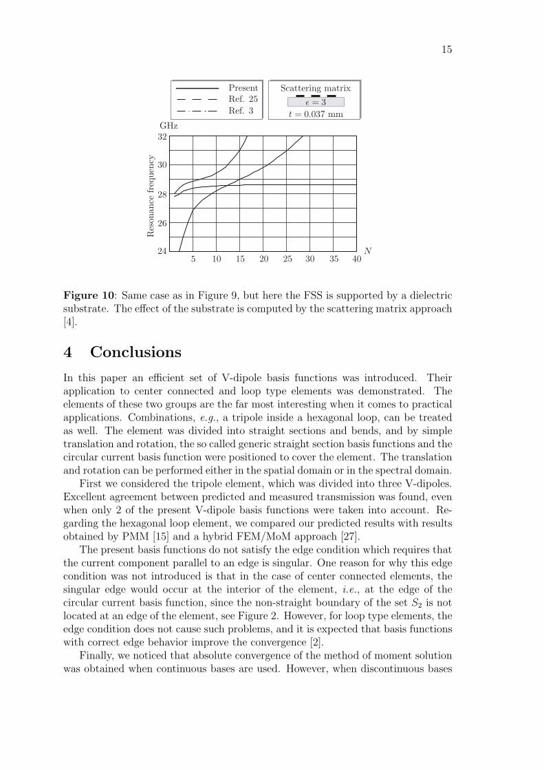
We now investigate the convergence when the FSS is supported by a substrate. InFigure 10 the substrate is taken into account by the scattering matrix approach [4].We include Floquet waves (plane waves) up to order 4, i.e., the size of the scatteringmatrices is 162× 162. Again, absolute convergence is found for the present base. Infact, the convergence results are similar to the ones obtained for the free standingFSS. This is not surprising, since in the scattering matrix approach, we first calculatethe scattering matrices for the free standing FSS and substrate, respectively, andthen the scattering matrix of the cascaded structure is obtained by simple matrix

14

5 10 15 20 25 30 35 4024

26

28

30

32GHz

N

Res

onan

cefr

eque

ncy

Ref. 3

PresentRef. 25 No substrate

Figure 9: The resonance frequency vs. the number of Floquet modes included forthe tripole array of Figure 6, but without the dielectric substrate. The angles ofincidence are θ = 45◦ and φ = 90◦.

algebra. However, when using the full wave method [11, 12], the current distributionfound by the method of moments is calculated with the substrate present. Hence, theconvergence of the double infinite Floquet sums is affected by the actual substrate. InFigure 11 the convergence is shown when the full wave method is used. Convergenceis found for the present base, and the resonance frequency converges to f1 = 27GHz as the number of Floquet modes approaches infinity. Hence, the resonancefrequency is reduced 8.5% when the substrate is introduced, see Figure 9. Whenusing the scattering matrix approach, see Figure 10, the resonance frequency wasreduced 3% only. It is found that the discrepancy, 8.5% compared to 3% reduction,is reduced when more Floquet waves (plane waves) are included. However, thatwould require larger scattering matrices, and due to computer limitations, we havenot been able to investigate the effect of including more Floquet waves. The size ofthe scattering matrices is 2(2M + 1)2 × 2(2M + 1)2, where M is the index of thehighest order Floquet wave included. This poor convergence of the scattering matrixapproach can be avoided by letting a part of the substrate support the FSS, suchthat the evanescent waves radiated from the FSS are suppressed in the supportingsubstrate [22].

Numerous methods have been used to analyze FSSs. It is important to noticethat the convergence results given here is valid for the spectral Galerkin method [24],and that they are not necessarily true for other methods, for instance the equivalentcircuit method.

15

5 10 15 20 25 30 35 4024

26

28

30

32GHz

N

Res

onan

cefr

eque

ncy

Ref. 3

PresentRef. 25

Scattering matrix

ε = 3t = 0.037 mm

Figure 10: Same case as in Figure 9, but here the FSS is supported by a dielectricsubstrate. The effect of the substrate is computed by the scattering matrix approach[4].

4 Conclusions

In this paper an efficient set of V-dipole basis functions was introduced. Theirapplication to center connected and loop type elements was demonstrated. Theelements of these two groups are the far most interesting when it comes to practicalapplications. Combinations, e.g., a tripole inside a hexagonal loop, can be treatedas well. The element was divided into straight sections and bends, and by simpletranslation and rotation, the so called generic straight section basis functions and thecircular current basis function were positioned to cover the element. The translationand rotation can be performed either in the spatial domain or in the spectral domain.

First we considered the tripole element, which was divided into three V-dipoles.Excellent agreement between predicted and measured transmission was found, evenwhen only 2 of the present V-dipole basis functions were taken into account. Re-garding the hexagonal loop element, we compared our predicted results with resultsobtained by PMM [15] and a hybrid FEM/MoM approach [27].

The present basis functions do not satisfy the edge condition which requires thatthe current component parallel to an edge is singular. One reason for why this edgecondition was not introduced is that in the case of center connected elements, thesingular edge would occur at the interior of the element, i.e., at the edge of thecircular current basis function, since the non-straight boundary of the set S2 is notlocated at an edge of the element, see Figure 2. However, for loop type elements, theedge condition does not cause such problems, and it is expected that basis functionswith correct edge behavior improve the convergence [2].

Finally, we noticed that absolute convergence of the method of moment solutionwas obtained when continuous bases are used. However, when discontinuous bases

16

5 10 15 20 25 30 35 4024

26

28

30

32GHz

N

Res

onan

cefr

eque

ncy

Ref. 3

PresentRef. 25

Full wave

ε = 3t = 0.037 mm

Figure 11: Same case as in Figure 10, but here the effect of the substrate iscomputed by the full wave approach [11].

are used, the method of moment solution does not converge as the number of Floquetmodes are increased. In fact, we found that the double infinite Floquet sum divergeswhen discontinuous bases are used. Therefore, care needs to be exercised and itwould seem discontinuous bases should be avoided.

Appendix A The Fourier transform

The Fourier transform of the circular current basis function is given by

jc(τ ; v) :=

∫Sc

−xy + yx√x2 + y2

e−iρ·τ dx dy

In polar coordinates ρ and φ, this integral can be written

jc(τ ; v) =

∫ W

0

ρ dρ

∫ v

0

dφ{−x sinφ + y cosφ

}e−iρτ cos(φ−ϕ)

where τ = xτ cosϕ + yτ sinϕ. We substitute ξ = φ− ϕ and notice that{sin(ξ + ϕ) = sin ξ cosϕ + cos ξ sinϕ

cos(ξ + ϕ) = cos ξ cosϕ− sin ξ sinϕ

The result is

jc(τ ; v) =

∫ W

0

ρ dρ

∫ ϕ

ϕ−vdξ

{x(sin ξ cosϕ− cos ξ sinϕ)

+ y(cos ξ cosϕ + sin ξ sinϕ)}e−iρτ cos ξ

=

∫ W

0

ρ dρ

∫ ϕ

ϕ−vdξ

{τ sin ξ + ϕ cos ξ

}e−iρτ cos ξ

17

where τ := x cosϕ + y sinϕ and ϕ := −x sinϕ + y cosϕ. Two integrals can beidentified, jcτ (τ ; v) and jcϕ(τ ; v), such that

jc(τ ; v) = τ jcτ (τ ; v) + ϕjcϕ(τ ; v)

The integral jcτ (τ ; v) can be performed in closed form,

jcτ (τ ; v) :=

∫ W

0

ρ dρ

∫ ϕ

ϕ−vdξ sin ξ e−iρτ cos ξ

= Γ2(ϕ)− Γ2(ϕ− v)

where Γ2(ξ) := (e−iWτ cos ξ − 1)/τ 2 cos ξ. The integral jcϕ(τ ; v) is defined as

jcϕ(τ ; v) :=

∫ W

0

ρ dρ

∫ ϕ

ϕ−vdξ cos ξ e−iρτ cos ξ

We perform the integration over ρ and get

jcϕ(τ ; v) =1

τ 2

∫ ϕ

ϕ−v

(iWτe−iWτ cos ξ +

e−iWτ cos ξ − 1

cos ξ

)dξ

This integral is performed by numerical integration. Notice that the Fourier trans-form of the basis functions can be computed and stored once in the beginning ofthe computation. Finally, the Fourier transform of the generic straight section basisfunctions j+,◦

p (ρ;xs, xe), see (2.1), is easily expressed in closed form.

Appendix Acknowledgments

I am deeply grateful to my supervisor prof. Gerhard Kristensson, and would like tothank him for his excellent guidance throughout this work. I would also like to thankBjorn Widenberg for providing the hybrid FEM/MoM results which we use here forcomparison. Furthermore, I am deeply grateful to prof. Ben Munk for the invitationto work in his group at the ElectroScience Laboratory, Ohio State University. Thework reported in this paper is supported by a grant from the Defence MaterielAdministration of Sweden (FMV) and its support is gratefully acknowledged.

References

[1] M. Akerberg. Scattering from frequency selective surfaces: A set of basis func-tions for the tripole loop. Master’s thesis, Lund Institute of Technology, De-partment of Electroscience, P.O. Box 118, SE-211 00 Lund, Sweden, 1999. Tech.Rep. LUTEDX/(TEAT-5032)/1–34/(1999).

[2] T. Andersson. Moment-method calculations on apertures using basis singularfunctions. IEEE Trans. Antennas Propagat., 41(12), 1709–1716, 1993.

18

[3] P. W. B. Au et al. Parametric study of tripole and tripole loop arrays as fre-quency selective surfaces. IEE Proc.-H Microwaves, Antennas and Propagation,137(5), 263–268, 1990.

[4] T. A. Cwik and R. Mittra. The cascade connection of planar periodic surfacesand lossy dielectric layers to form an arbitrary periodic screen. IEEE Trans.Antennas Propagat., 35(12), 1397–1405, December 1987.

[5] T. A. Cwik and R. Mittra. Correction to “The cascade connection of planar pe-riodic surfaces and lossy dielectric layers to form an arbitrary periodic screen”.IEEE Trans. Antennas Propagat., 36(9), 1335, September 1988.

[6] J. G. Gallagher and D. J. Brammer. High order resonances and scattering fromFSS tripole arrays. In Proc. 6th Int. Conf. on Antennas and Propagation, IEEConf. Publ., pages 521–525, 1989.

[7] R. C. Hall, R. Mittra, and K. M. Mitzner. Analysis of multilayered periodicstructures using generalized scattering matrix-theory. IEEE Trans. AntennasPropagat., 36(4), 511–518, 1988.

[8] L. W. Henderson. Introduction to PMM, version 4.0. Technical Report 725347-1, ElectroScience Laboratory, Ohio State University, Department of ElectricalEngineering, 1320 Kinnear Road, Columbus, Ohio 43212, USA, 1993.

[9] W. A. Imbraile, V. Galindo-Israel, and Y. Rahmat-Samii. On the reflectivityof complex mesh surfaces. IEEE Trans. Antennas Propagat., 39, 1352–1365,September 1991.

[10] F. S. Johansson. Convergence phenomenon in the solution of dichroic scatter-ing problems by Galerkin’s method. IEE Proc.-H Microwaves, Antennas andPropagation, 134, 87–92, February 1987.

[11] G. Kristensson, M. Akerberg, and S. Poulsen. Scattering from a frequencyselective surface supported by a bianisotropic substrate. In J. A. Kong, editor,Electromagnetic Waves PIER 35, pages 83–114. EMW Publishing, Cambridge,Massachusetts, 2001.

[12] G. Kristensson, S. Poulsen, and S. Rikte. Propagators and scattering of elec-tromagnetic waves in planar bianisotropic slabs — an application to frequencyselective structures. Technical Report LUTEDX/(TEAT-7099)/1–32/(2001),Lund Institute of Technology, Department of Electroscience, P.O. Box 118,S-211 00 Lund, Sweden, 2001.

[13] R. Mittra. Relative convergence of the solution of a doubly infinite set ofequations. J. Nat. Bur. Stand., 67D, 245–254, Mar.–Apr. 1963.

[14] M. M. Mokhtar and E. A. Parker. Conjugate-gradient computation of thecurrent distribution on a tripole FSS array element. Electronics Letters, 26(4),227–228, 1990.

19

[15] B. Munk. Frequency Selective Surfaces: Theory and Design. John Wiley &Sons, New York, 2000.

[16] B. A. Munk and G. A. Burrell. Plane-wave expansion for arrays of arbitrarilyoriented piecewise linear elements and its application in determining the im-pedance of a single linear antenna in a lossy half-space. IEEE Trans. AntennasPropagat., 27(3), 331–343, 1979.

[17] B. A. Munk, G. A. Burrell, and T. W. Kornbau. A general theory of peri-odic surfaces in stratified media. Technical Report 784346-1, ElectroScienceLaboratory, Ohio State University, Department of Electrical Engineering, 1320Kinnear Road, Columbus, Ohio 43212, USA, 1977. Prepared under contractAFAL-TR-77-219.

[18] L. Musa et al. Sensitivity of tripole and calthrop FSS reflection bands to angleof incidence. Electronics Letters, 25(4), 284–285, 1989.

[19] S. Poulsen. Scattering from frequency selective surfaces: A continuity conditionfor entire domain basis functions and an improved set of basis functions forcrossed dipole. IEE Proc.-H Microwaves, Antennas and Propagation, 146(3),234–240, 1999.

[20] S. Poulsen. Scattering of electromagnetic waves from frequency selective sur-faces. Licentiate thesis, Lund Institute of Technology, Department of AppliedElectronics, Electromagnetic Theory, P.O. Box 118, S-211 00 Lund, Sweden,2000.

[21] L. S. Riggs and R. G. Smith. Efficient current expansion modes for the triarmfrequency-selective surface. IEEE Trans. Antennas Propagat., 36(8), 1172–1177, 1988.

[22] N. V. Shuley. Higher-order mode interaction in planar periodic structures. IEEProceedings, 131(3), 129–132, June 1984.

[23] N. V. Shuley. A note on relative convergence for moment-method solutions ofintegral equations of the first kind as applied to dichroic problems. ElectronicsLetters, 21(3), 95–97, 1985.

[24] C.-H. Tsao and R. Mittra. Spectral-domain analysis of frequency selectivesurfaces comprised of periodic arrays of cross dipoles and Jerusalem crosses.IEEE Trans. Antennas Propagat., 32(5), 478–486, 1984.

[25] J. C. Vardaxoglou and E. A. Parker. Performance of two tripole arrays asfrequency-selective surfaces. Electronics Letters, 19(18), 709–710, 1983.

[26] K. J. Webb, P. W. Grounds, and R. Mittra. Convergence in the spectral do-main formulation of waveguide and scattering problems. IEEE Trans. AntennasPropagat., 38, 869–877, June 1990.

20

[27] B. Widenberg, S. Poulsen, and A. Karlsson. Scattering from thick frequencyselective screens. J. Electro. Waves Applic., 14, 1303–1328, 2000.

[28] T. K. Wu, editor. Frequency Selective Surface and Grid Array. John Wiley &Sons, New York, 1995.