possibility of designing a practical multiplier chip which attains these bounds remains open.

Received April 1979; revised August 1979; accepted October 1979

References I. Abelson, H. Lower bounds on information transfer in distributed systems. Proc. 19th IEEE Seminar Foundations Comptr. Sci., Ann Arbor, Mich., 1978. 2. Brent, R.P., and Kung, H.T. The area-time complexity of binary multiplication. Tech. Rep., Dept. Comptr. Sci., Carnegie-Mellon U., Pittsburgh, Pa., July 1979. 3. Preparata, F.P., and Vuillemin, J. The cube-connected-cycles: A versatile network. Proc. 20th IEEE Seminar Foundations Comptr. Sci., 1979. 4. Savage, J.E., and Swamy, S. Space-time tradeoffs for oblivious sorting and integer multiplication. Tech. Rep. No. 37, Dept. of Comptr. Sci., Brown U., Providence, R.I., 1978. 5. Thompson, C.D. Area-time complexity for VLSI. Proc. 1 lth Ann. ACM Symp. Theory of Comptg., Atlanta, Ga., April-May 1979, pp. 81-88. 6. VuiUemin, J.P. A note on the paper: Area-time complexity for VLSI. Institute pour Recherche d'Infomatique et d'Automatique, Rocqencourt, France, 1979 (unpublished note). 7. Wallace, C.S. A suggestion for a fast multiplier. IEEE Trans. Electronic Comptg. EC-13 (Feb. 1964), 14-17.

Graphics and J.D. Foley Image Processing Editor

Scan Line Methods for Displaying Parametrlcalb Y Defined Surfaces Jeffrey M. Lane Boeing Commercial Airplane Company

Loren C. Carpenter Boeing Computer Services

Turner Whitted Bell Laboratories

James F. Blinn Caltech/JPL

23

This paper presents three scan line methods for drawing pictures of parametrically defined surfaces. A scan line algorithm is characterized by the order in which it generates the picture elements of the image. These are generated left to right, top to bottom in much the same way as a picture is scanned out on a TV screen. Parametrically defined surfaces are those generated by a set of bivariate functions defining the X, Y, and Z position of points on the surface. The primary driving mechanism behind such an algorithm is the inversion of the functions used to define the surface. In this paper, three different methods for doing the numerical inversion are presented along with an overview of scan line methods.

Key Words and Phrases: computer graphics, scan line algorithm, shaded graphics display, parametric surfaces

CR Categories: 5.12, 5.13, 8.1, 8.2 Permission to copy without fee all or part of this material is

granted provided that the copies are not made or distributed for direct commercial advantage, the ACM copyright notice and the title of the publication and its date appear, and notice is given that copying is by permission of the Association for Computing Machinery. To copy otherwise, or to republish, requires a fee and/or specific permission.

Turner Whitted's work was performed at North Carolina State University, Raleigh, N.C., and was supported in part by the National Science Foundation under grant MCS 75-06599.

Authors' present addresses: J.F. Blinn, Jet Propulsion Laboratory, 4800 Oak Grove Dr., 125-104, Pasadena, CA 91103; L.C. Carpenter and J.M. Lane, Mail Stop 35-02, The Boeing Company, P.O. Box 3707, Seattle, WA 98124; T. Whitted, Bell Telephone Labs., Room 4F621, Holmdel, NJ 07733. © 1980 ACM 0001-0782/80/0100-0023 $00.75.

Communications January 1980 of Volume 23 the ACM Number 1

1. Introduction

Computer aided design has long been concerned with the design of parametrically representable surfaces. Such surfaces are those defined by three bivariate functions:

X = X(u, v) Y = Y(u, v) Z = Z(u, v)

As the parameters vary between 0 and 1, the functions sweep out the surface in question. The mathematical representation of these surfaces provides shapes with pleasing properties of continuity and smoothness. Until recently, the only method for drawing shaded pictures of such a surface has been to divide it into many polygonal facets and to apply any of several polygon drawing algorithms. A few years ago, Catmull [3] devised one of the first algorithms for drawing bicubic parametric sur- faces directly from the mathematical surface formula- tion. While this algorithm generates images of superior quality, it still has some drawbacks. These have to do with speed and memory requirements and the ease of performing anti-aliasing operations. These drawbacks are eliminated by the class of algorithms known as scan line algorithms. Such algorithms generate the picture elements in order from left to right, top to bottom on the screen, much as a television might scan them out. The algorithms described here are scan line based algorithms for generating such images which remove some of the difficulties of Catmull's algorithm without substantial sacrifice in picture quality. Before presenting the new methods, however, it will be useful to review scan line techniques for polygonal objects.

2. Scan Line Algorithms

Each of the new algorithms is a generalization of more conventional scan line algorithms for drawing poly- gonal objects. It is therefore worthwhile to examine conceptually what is happening during a scan line algo- rithm for polygons. It is assumed for both the polygonal case and the parametric curve case that the objects to be drawn have been transformed to a screen space with X going to the right, Y going up, and Z going into the screen. Furthermore, the perspective transformation is assumed to have been performed on all objects as de-

Editor's Note: This is a combination of three individual papers previously accepted for publication in Communications of the A CM. The papers were "A Scan Line Algorithm for the Computer Display of Parametrically Defined Surfaces" by J. Lane and L. Carpenter, "A Scan Line Algorithm for Displaying Parametrically Defined Surfaces" by J. Blinn, and "A Scan Line Algorithm for Computer Display of Curved Surfaces" by T. Whitted. The latter two papers were presented at SIGGRAPH '78. The section editor is grateful to J. Blinn for suggesting that the papers be merged, and to J. Lane for managing the production of the new paper.--J.D. Foley

24

scribed in [6, 14] so that an orthographic projection of X and Y onto the screen is appropriate. In the case of parametric curved surfaces this serves to alter the form of the functions somewhat but the processing performed upon those functions remains the same.

A scan line algorithm basically consists of two nested loops, one for the Y coordinate going down the screen and one for the X coordinate going across each scan line of the current Y. For each execution of the Y loop, a plane is defined by the eyepoint and the scan line on the screen. All objects to be drawn are intersected with this plane. The result is a set of line segments in XZ, one (or more) for each potentially visible polygon on that scan line. These fine segments are then processed by the X scan loop. For each execution of this loop a scan ray is defined by the eyepoint and a picture element on the screen. All segments are intersected with this ray to yield a set of points, one for each potentially visible polygon at that picture element. These points are then sorted by their Z position. The point with the smallest Z is deemed visible and an intensity is computed for it. The processing during the X scan is, then, fundamentally the same as the processing during the Y scan except for the change in dimensionality. During the Y scan, 3D polygons are intersected with a plane to produce 2D fine segments. During the X scan, 2D line segments are intersected with a line to produce 1D points.

Many enhancements must be added to the basic scheme to make it practical. Most of these are referred to as taking advantage of the "coherence" of the picture. This basically means that many of the calculations are made incremental rather than absolute. The opportunity to do this is, indeed, much more the reason for generating pictures in scan line order in the first place. For example, the Y scan is responsible for constructing a list of all potentially visible segments which will be processed by the X scan. Rather than construct this list from scratch for each Y coordinate, it is usual to keep the list around between scan lines and update it according to how it has changed. Changes to this "active segment fist" take three forms. As the scan plane drops below a vertex of the polygon which represents a local maximum, a new seg- ment must be created and added to the list, Figure l(a). As the scan plane drops below a vertex which represents a local minimum, a segment must be deleted from the list, Figure l(b). Finally, for those segments which re- main in the fist, X Z coordinates of the endpoints of the segments must be updated to reflect their new position, Figure l(c).

This latter operation can also be computed incremen- tally. The endpoint of an active segment is generated by the intersection of an edge of the polygon (a straight line segment) with the scan plane. The amounts of change in X and Z for a unit step in Y are constants along the entirety of the edge. The increments can be computed once when the edge first becomes active and just added to the X Z position for each step in Y.

Communications January 1980 of Volume 23 the ACM Number 1

Fig. 1. Incremental scan line operations.

(a)

Scan line passes local maximum

f (b)

Scan line passes local minimum

(c) Change in X, Z for normal update

The computation for the Y loop then reduces to the following processes. All endpoints are initially sorted in Y to determine the order in which they will pass through the Y scan plane. For each new Y, the X and Z coordi- nates of all existing segments are updated. If any polygon vertices have been passed, new segments are created or old ones deleted according to the type of vertex. The calculations are analogously made incremental for the X scan. As it proceeds, it maintains its own "active point list" of intersections. We consider the X scan process in more detail in the next section.

2.1 X-Z Plane Processing Each of the algorithms described here, like polygon

algorithms, generates a list of sample points in the X-Z

25

plane for every scan line. The sample points are linked in pairs by straight lines to form scan line segments, which are a piecewise linear approximation to the curve of intersection between the X-Z scanning plane and the surface element being displayed. The ways in which these segments are formed varies considerably between the various algorithms. The further processing of these segments, i.e., the transformation from segments to pix- els, makes use of common shading techniques which can be applied to any of the algorithms. We will discuss shading techniques further in Section 2.2.

The visible surface algorithm scans line segments to resolve the two final unknowns in the display process: (1) which scan line segments or portions of segments are visible, and (2) what intensity value must be applied to each pixel along a visible segment.

2.1.1 Z before X sorting. Conceptually, visibility is easy to determine: Whatever surface lies closest to the viewer at any given point is the visible one. One way to actually calculate the visibility is to sort all surfaces with respect to their distance from the viewer and assign a priority to each surface based on the order of the sorted list [3]. If the priority cannot be resolved, then the surfaces must be subdivided until an unambiguous or- dering is found. Then at each point along a scan line, the segment belonging to the highest priority surface is the visible one. A simpler technique is to wait until after the list of scan line segments has been generated to determine priority. Then the sort can be made in the X- Z plane with less chance of ambiguities.

Alternatively, an algorithm may paint each scan line segment into a pixel buffer, starting with the farthest segment and ending with the nearest. If any segment overlaps another that has been previously written, it will overwrite the previous one. In this way the nearest surface will be visible in the final image. To display transparent surfaces, near surfaces only partially over- write the background. This priority technique has the disadvantage that each scan line segment must be painted whether it is visible or not.

When displaying opaque surfaces, it is not necessary to know the entire ordering of segments; it is sufficient to know just which one has the highest priority. A simple way of determining this uses a "z-buffer" (an array containing as many locations as the scan line does pixels) [1, 4]. The z-buffer is initialized to the depth of the far clipping plane. Then as each segment is processed, its depth is compared to the value stored in the z-buffer. If the new depth is greater than the currently visible one, the new segment is not visible at that point. If the new depth is less than the currently visible one, the new depth value is written into the z-buffer and the intensity value calculated for the current segment at that point over- writes the previous value. In this manner the nearest segment will always be visible regardless of the order in which segments were processed.

Communications January 1980 of Volume 23 the ACM Number 1

2.1.2 X before Z sorting. Instead of sorting segments according to depth (Z dimension), it is sometimes more convenient to sort according to the X value of the left- most endpoint and let the processing move from left to right along the scan line. The shading processor will add a segment to its actiye list as soon as the X value of its left endpoint is less than the X value of the current pixel. If the new segment is in front of the currently visible segment, then the new one is declared visible. It remains visible until it intersects another active segment or is obscured by a newly active segment. By processing seg- ments in this order, the shader considers only the visible surfaces and saves a considerable amount of time.

2.1.3 Scan line coherence. An alternative to sorting in X and Z is to simply write each segment into a scan line z-buffer, where a pixel is overwritten only if the new z value is in front of the old z value as in [10]. X before Z sorting is employed in the first algorithm below, Z before X is employed in the second, and the third algo- rithm uses the scanline z-buffer technique.

The above discussion refers to the order of processing, and to visibility calculations. The remaining processing, called shading, will assign an intensity value to each point once it is declared visible.

2.2 Intensity Computation It is known that the reflected light received by an

observer from any point on an object depends on the angle between the direction of sight and the reflected light vector at that point. This dependency may be modeled in many different ways in synthetic images. Gouraud [5] determined intensity at a point on a surface by

(2.2. l) Intensity = s(L. N )

where s is a reflectance factor, L is the unit light source vector, N is the unit normal vector, and • denotes the vector "dot" product. Phong [7] improved this model to approximate highlights

(2.2.2) Intensity = s ( L . N ) + g ( V . N ) n

where V is a unit virtual light source direction, g is a measure of the glossiness, and n > 1. Further work on mathematical models for intensity calculation has been done by Blinn [1].

Blinn noted that the proportion of specular reflection g varies with the direction of the light source, and the direction of maximum reflection is not always exactly along V. In his model Blinn assumes the surface being simulated is composed of a collection of highly reflective microfacets oriented randomly on the surface. His math- ematical model for intensity then becomes

(2.2.3) Intensity = s ( L . N ) + g( l - s)

where

26

DGF

g - ( N . E ) ' D is the distribution function of the directions of the

microfacets of the surface, G is the amount by which the facets shadow and mask

each other, E is the eye direction, and F is the Fresnel reflection law.

The Gouraud model was used in shading the figures in Section 5, the Phong model was used in Section 4, and the Blinn model in Section 3.

3. Blinn Algorithm

This algorithm generalizes the concept of scanning a polygon to scanning a surface patch. The relevant prop- erties of polygons which make them scannable are:

(a) We can determine Y-maxima/minima from the cor- ner points and sort on Y coordinate.

(b) We can track edges as functions of Y. (c) Each scan line segment is scannable in Z as a func-

tion of X.

Parametric surfaces have none of these properties. The Y-maxima/minima can occur on the boundary or the interior of the patch, and we need to distinguish between local and global maxima/minima. Not only do we need to track the boundary edges, but we need to track silhouette edges as well. For smooth surfaces the silhou- ette edges correspond to curves in the surface where the Z-component of the normal is zero. (See Figure 2.) These curves may or may not intersect the boundary of the patch. Neither the boundary nor the silhouette edges need be monotonic in Y, or representable as a function of Y. Similar problems exist for each X scan.

Although for parametric surface patches the Y-max- ima/minima and edge information is not readily avail- able, one can approximate this data with iterative tech- niques [14]. The relevant systems of equations are:

For determining boundary curve interactions with the current scan line (Y scan):

(a) Y(0, v) = Yscan, (b) Y(1, v) = Yscan, (c) r (u , 0) -- Yscan, (d) Y(u, 1)= Yscan.

For determining silhouette edge intersections with the current scan line:

Y (u, v) = Yscan Zn(u, v) = 0

where Zn(u, v) is the Z component of the normal equa- tion of the patch.

For determining local Y maxima/minima:

Yu(u, v) = 0 Yv(u, v) = 0

Communications January 1980 of Volume 23 the ACM Number 1

Fig. 2. Two Types of Edges for Curved Surfaces.

. . . .

SILHOUETTE---~

(a) (b)

~'~I~J~BOUNDARV

~ BOUNDARY

l~x

where Yu and Yv are the partials with respect to u and v.

For determining segments of the x scan:

Y(u, v) - Yscan = 0 X(u, v) - Xscan = 0.

Newton iteration is a useful technique for solving each of these systems [14]. In particular, since Newton itera- tion requires an initial guess at a solution, a type of coherence can be built into the tracking mechanism if we use the previous (u, v) solution as a guess for the current scan line. As with polygons, edges are created at Y maxima and at the intersection of boundary and silhouette edges. Similarly, edges are deleted at Y minima and intersections with boundary edges. By inserting sil- houette edges and partitioning all edges with Y maxima/ minima, we have effectively partitioned the surface patch itself into pieces which are monotonic decreasing in Y and singularly valued in Z. This information is used during the X scan to produce the front most point on the surface for any (X scan, Y scan) point.

Problems with this approach would appear to be numerous. Singularities or cusps in the patch and its derivatives can occur even though the surface is analytic as a function of (u, v). For these cases Newton iteration is not appropriate and other iterative or heuristic ap- proaches have to be used. There can be many types of Y maxima/minima such as saddle points, which induce the creation of additional edges, and the problem of resolv- ing multiple condition points, such as a silhouette edge starting at a boundary point where a maxima also occurs, are always present. More details on special cases can be found in [1]. However, for most models of three-dimen- sional shapes the surface pieces tend to be well-behaved, and for these surfaces this algorithm has proven robust and relevant.

27

4. Whitted Algorithm

A second algorithm for surface display is also a generalization of polygon type algorithms. In it, patches are described in terms of edges, which in this case are cubic curves instead of straight lines. These edges are intersected by successive scanning planes to form the endpoints of scan line segments that are passed to the shader.

This approach fails naturally, if the surface element contains a silhouette on its interior or if it is excessively curved. To circumvent this problem the processor that generates edges also detects silhouettes and divides the patch along the silhouette curve. If a patch is excessively curved, the edge generator can produce additional curves on the interior of the patch to improve the accuracy of the image.

4.1 Edge Description of Patches Bicubic surface patches have four natural edge

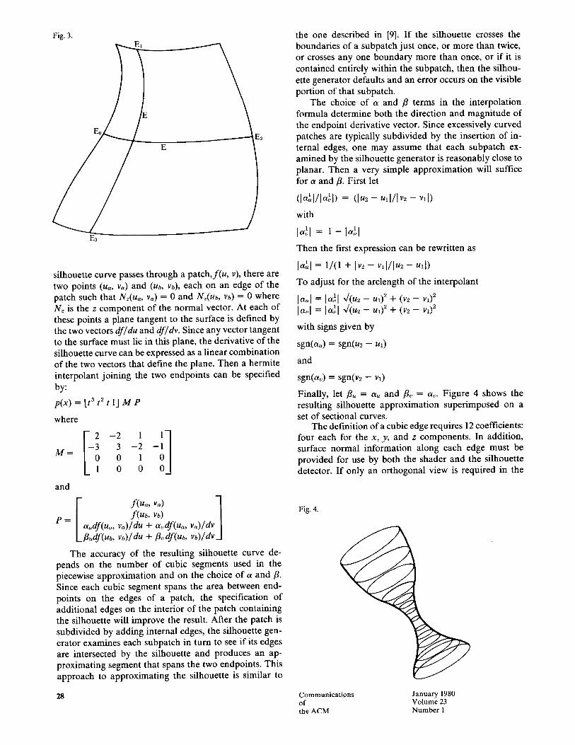
curves: E0 = f (u , 0), E1 = F(O, v), E2 = f (u , 1), and E3 = f ( l , v), each of which is cubic in one variable. If, as in the case of excessively curved patches, it is necessary to specify additional "edges" on the interior of the patch, these edges (parametric curves on the surface) are also cubic curves of one variable, defined by either E~ = f ( k , , v) or E~ =f(u , ku). The addition of two such interior edges, specified by ku = 0.5 and kv = 0.5, has the effect of dividing the patch into four subpatches, as shown in Figure 3.

A third type of edge is the patch silhouette, i.e., the curve on the surface for which the z component of the normal vector is zero. In general, the order of the silhou- ette curve is greater than the cubic, but it is approximated here by a piecewise cubic interpolant so that the silhou- ette can be treated the same as any other edge. If the

Communications January 1980 of Volume 23 the ACM Number 1

E3

_/

by:

p(x) = [t 3 t 2 t 1] M P

where

M = 3 - 2 0 1 0 0

silhouette curve passes through a pa t ch , f (u, v), there are two points (ua, va) and (ub, Vb), each on an edge of the patch such that Nz(ua, va) = 0 and Nz(Ub, Vb) = 0 where Nz is the z component of the normal vector. At each of these points a plane tangent to the surface is defined by the two vectors df/du and df/dv. Since any vector tangent to the surface must lie in this plane, the derivative of the silhouette curve can be expressed as a linear combination of the two vectors that define the plane. Then a hermite interpolant joining the two endpoints can be specified

and

p =

28

il f(Ua, Vo) ] f(ub, v~)

a,df(ua, Va)/du + avdf(ua, v,,)/dv Lfudf(ub, Vb)/du + flodf(ub, Vb)/dv_l

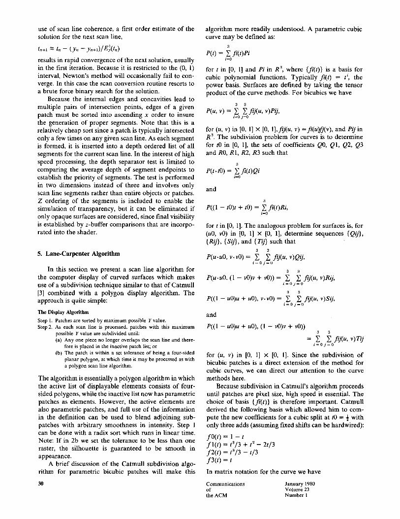
The accuracy of the resulting silhouette curve de- pends on the number of cubic segments used in the piecewise approximation and on the choice of a and ft. Since each cubic segment spans the area between end- points on the edges of a patch, the specification of additional edges on the interior of the patch containing the silhouette will improve the result. After the patch is subdivided by adding internal edges, the silhouette gen- erator examines each subpatch in turn to see if its edges are intersected by the silhouette and produces an ap- proximating segment that spans the two endpoints. This approach to approximating the silhouette is similar to

Communications of the ACM

the one described in [9]. If the silhouette crosses the boundaries of a subpatch just once, or more than twice, or crosses any one boundary more than once, or if it is contained entirely within the subpatch, then the silhou- ette generator defaults and an error occurs on the visible portion of that subpatch.

The choice of a and fl terms in the interpolation formula determine both the direction and magnitude of the endpoint derivative vector. Since excessively curved patches are typically subdivided by the insertion of in- ternal edges, one may assume that each subpatch ex- amined by the silhouette generator is reasonably close to planar. Then a very simple approximation will suffice for a and ft. First let

al ogl (I , , I / I ol) = ( lu~ - u , I / I v ~ - vi i )

with

Og 1 I~1= 1 - 1 ul

Then the first expression can be rewritten as

I~11 = 1 / ( 1 + Iv2 - - v , I / l . 2 - u ,I )

To adjust for the arclength of the interpolant

l a . I = l a~l 4(u2 - u,) ~ + (v2 - v,) 2 lavl = laLI . / (u2 - u , ) ~ + (v~ - P 1 ) 2

with signs given by

sgn(a,) = sgn(u2 - ul)

and

sgn(ao) = sgn(v2 - Va)

Finally, let flu = au and fly = av. Figure 4 shows the resulting silhouette approximation superimposed on a set of sectional curves.

The definition of a cubic edge requires 12 coefficients: four each for the x, y, and z components. In addition, surface normal information along each edge must be provided for use by both the shader and the silhouette detector. If only an orthogonal view is required in the

Fig. 4.

January 1980 Volume 23 Number 1

Fig. 3.

E2

Fig. 5.

(a) " ~ I

final display, all of the required information can be obtained from the coefficients of the derivative with respect to the constant parameter along each edge. 1 The derivative with respect to the variable parameter (the curve's tangent vector) can be derived readily from the curve coefficients. The cross-product of these two deriv- atives yields an exact normal at each point on the edge.

Ordinarily a perspective view is required. A tech- nique described by Catmull [3] uses a bicubic equation to approximate the cubic normal function along each edge. The perspective view of the surface is generated by transforming the control points for the surface and using the resulting control points to form an approximation to the transformed bicubic surface. The bicubic normal approximation is not passed through the perspective transform since proper shading depends on preserving the object space illumination direction. Use of the ap- proximate normal function has the added advantage of speeding the scan conversion process since it is not necessary to calculate cross-products at every intersection point on the edge to find the surface normal.

Edges are stored in a y-sorted list of modules, each containing 24 coefficients (12 for the edge curve and 12 for the cubic normal approximation). As noted before, the inclusion of interior edges effectively subdivides the surface into smaller and more nearly planar subpatches.

There are interesting differences between this ap- proach and the subdivision of patches for approximation by polygons. Figure 5 shows a polygonal approximation of a bicubic patch created by evaluating the patch equa- tion at 25 equally spaced vertex points. Assuming that the patch is surrounded by four neighbors with which it shares vertices and edges, the number of vertices per patch is 16 and the number of edges is 32. Each vertex

On the edge Eu =f(u k,,), df/dv is a cubic function with respect to u.

29

is defined by six coefficients (three for position and three for the surface normal) and each edge description re- quires two pointers (one to each of the endpoint vertices). The total number of words required per patch is 160. Figure 5 shows the same patch in terms of its boundary curves and six internal edges. Assuming that the bound- aries are shared, the total number of edges per patch is eight, requiring 192 words of memory. In general, if a patch is subdivided M times in the u direction and N times in the v direction and represented by quadrilateral polygons, the number of edges required is 2 M N per patch. For the approach given here only M + N cubic edges are required. (In Figure 5, M = 4 and N = 4). Furthermore, every cubic edge lies entirely on the surface (except for the silhouette approximation) whereas if a polygonal approximation is used, the edges coincide with the surface only at the vertices.

4.2 Intersection Processor The intersection (scan conversion) processor is the

heart of this algorithm; it operates on the edge list and outputs scan line segments in reverse order of visibility.

The first stage of the procedure examines each edge to insure that it is monotonic in y, segmenting those that are not, and avoiding the problem of finding multiple intersections of the edge with a single scan line. The presence of extrema along an edge can be detected rapidly by examining the coefficients of the y component of the edge curve, and since the derivative of the curve is quadratic, their location is found using the quadratic formula to solve for zeros of the derivative.

The equation Ey(t) = yn where yn is the y value of scan line number and Ey(t) is the y component of the edge curve is solved using Newton's iteration to yield tn. In turn, Ex(tn), Ez(tn), and the components of the normal vector at that point on the edge are computed. Making

Communica t ions January 1980 of Volume 23 the ACM N u m b e r 1

use of scan line coherence, a first order estimate of the solution for the next scan line,

tn+l ~ tn - (yn - f ln+l) /El( tn)

results in rapid convergence of the next solution, usually in the first iteration. Because it is restricted to the (0, 1) interval, Newton's method will occasionally fail to con- verge. In this case the scan conversion routine resorts to a brute force binary search for the solution.

Because the internal edges and concavities lead to multiple pairs of intersection points, edges of a given patch must be sorted into ascending x order to insure the generation of proper segments. Note that this is a relatively cheap sort since a patch is typically intersected only a few times on any given scan line. As each segment is formed, it is inserted into a depth ordered list of all segments for the current scan line. In the interest of high speed processing, the depth separator test is limited to comparing the average depth of segment endpoints to establish the priority of segments. The test is performed in two dimensions instead of three and involves only scan line segments rather than entire objects or patches. Z ordering of the segments is included to enable the simulation of transparency, but it can be eliminated if only opaque surfaces are considered, since final visibility is established by z-buffer comparisons that are incorpo- rated into the shader.

5. Lane -Carpenter A l gor i thm

In this section we present a scan line algorithm for the computer display of curved surfaces which makes use of a subdivision technique similar to that of Catmull [3] combined with a polygon display algorithm. The approach is quite simple:

The Display Algorithm

Step I. Patches are sorted by m ax i mum possible Y value. Step 2. As each scan line is processed, patches with this m a x i m u m

possible Y value are subdivided until: (a) Any one piece no longer overlaps the scan line and there-

fore is placed in the inactive patch list; or (b) The patch is within a set tolerance of being a four-sided

planar polygon, at which time it may be processed as with a polygon scan line algorithm.

The algorithm is essentially a polygon algorithm in which the active list of displayable elements consists of four- sided polygons, while the inactive list now has parametric patches as elements. However, the active elements are also parametric patches, and full use of the information in the definition can be used to blend adjoining sub- patches with arbitrary smoothness in intensity. Step l can be done with a radix sort which runs in linear time. Note: If in 2b we set the tolerance to be less than one raster, the silhouette is guaranteed to be smooth in appearance.

A brief discussion of the Catmull subdivision algo- rithm for parametric bicubic patches will make this

30

algorithm more readily understood. A parametric cubic curve may be defined as:

3

P(t) = Y~ f i( t)Pi i=o

for t in [0, 1] and Pi in R 3, where {fi(t)} is a basis for cubic polynomial functions. Typically f i (0 = ti, the power basis. Surfaces are defined by taking the tensor product of the curve methods. For bicubics we have

3 3

P(u, v) = 2 • fij(u, v)e/j, i~0 j=0

for (u, v) in [0, 1] x [0, 1],fij(u, v) =fi(u)f j(v) , and P/J in R 3. The subdivision problem for curves is to determine for tO in [0, 1], the sets of coefficients Q0, QI, Q2, Q3 and R0, R1, R2, R3 such that

3

e(t . tO) = Y~ f i ( t )Qi i=0

and

3

P((1 - t0)t + to) = ~ f i( t)Ri, i=0

for t in [0, 1]. The analogous problem for surfaces is, for (u0, v0) in [0, 1] x [0, 1], determine sequences {Q/j}, {R/J}, {Sij}, and (Tij} such that

3 3

P(u.uO, v.vO) = ~ ~. fij(u, v)O/j, i = o j = 0

3 3

P(u.uO, (1 - vO)v + vO)) = ~ ~, fij(u, v)Rij, i = 0 j = O

3 3 e((1 - uO)u + uO), v.vO) = E Y, fij(u, v)si j ,

i = 0 j = 0

and

P((1 - uO)u + uO), (1 - vO)v + vO)) 3 3

= 2 2 fij(u, v)T/j i = O j = O

for (u, v) in [0, t] x [0, 1]. Since the subdivision of bicubic patches is a direct extension of the method for cubic curves, we can direct our attention to the curve methods here.

Because subdivision in Catmull's algorithm proceeds until patches are pixel size, high speed is essential. The choice of basis {fi(t)} is therefore important. Catmull derived the following basis which allowed him to com- pute the new coefficients for a cubic split at tO = ½ with only three adds (assuming fLxed shifts can be hardwired):

fO( t ) = 1 - t f l ( t ) = t3/3 + t z -- 2t/3 f2( t ) = t3/3 -- t /3 f3( t ) = t

In matrix notation for the curve we have

Communica t ions January 1980 of Volume 23 the ACM Number 1

± 0 P0 P(t) = [tat2t 1] 0 -½ a 0 1 0 P1 1 - 3 -½ P 2

1 0 0 P 3

Note P(0) = P0 and P(1) = P3. It is easily verified for the choice tO = ½ that

Q 0 = P 0 , R 0 = Q 3 , Ol = e l / 4 , R I -- 02 , 0 2 = ( P I + P 2 ) / 8 , R 2 = P 2 / 4 , 0 3 = ( P 0 + P 3 ) / 2 - ( P l + P 2 ) / 8 , R 3 = P 3 .

To the authors' knowledge there is no faster method to subdivide a parametric cubic polynomial at t = ½ than with the Catmull basis. However, the subdivision algo- rithm for display requires a subdivision of the patch and test for convergence. There does not seem to be a quick and accurate test for convergence with the Catmull basis which does not nullify the speed of the subdivision. For this reason we chose to use the Bernstein basis [31 for representing parametric cubics and bicubics.

The cubic Bernstein basis is given by

fO( t ) = (1 - t) a f l ( t ) = 3t(1 - t) z f2 ( t ) = 3(1 - t)t z f3 ( t ) = t 3

In matrix notation for the curve we have

As with Catmull's basis, P(0) = P0 and P(I) = P3. It can be verified for the choice tO = ½ that

Q0---P0 , R 0 = Q 3 Q1 = ( P 0 + P 1 ) / 2 , R1 = (P1 + P 2 ) / 4

+ R 2 / 2 Q 2 = Q I / 2 + ( P 1 + P 2 ) / 4 , R 2 = ( P 2 + P 3 ) / 2 Q3 = (02 + R1)/2 , R3 = P3

Thus with the Bernstein basis, subdivision of a cubic requires 6 adds. However, a very accurate and rapid convergence test is possible with this basis. Note that the basis functionsfi(t) are positive and sum identically to l, i.e.,

3

f i ( t ) >_ O, for all i and ~ f i ( t ) = 1, i=o

for t in [0, 1]. That is, every point of the curve lies within the convex hull of the coefficients Pi (see Figure 6). Thus the maximum Y of the curve (surface) is bounded by the maximum Y of the Pi (Pij) . From [l l] we know that the sequence of new coefficients converges to the curve (surface) as we continue to subdivide. Therefore we can use the length (area) of the convex hull of these'points to bound the length (area) of the curve (surface) segment (see Figure 7).

31

Fig. 6. Subdivision of cubic Bernstein polynomial.

I' 2

I' 3

We are now ready to discuss the implementation of the Display Algorithm. All surface patches are repre- sented in terms of the appropriate tensor product Bern- stein basis. Then Steps 1 and 2(a) are easily accomplished by testing the subpatch coefficients. The "flatness" test in Step 2(b) reduces to testing the "flatness" of the enclosing convex hull, both for the boundary curves being linear and the patch interior being planar. Lane and Riesenfeld have shown in [l l] that this convergence to linear polynomial form must take place. A simple flatness test for curve boundaries is to measure the distance of interior points on the convex hull to the line segment joining the end points. A similar test for surface flatness is to compute the distance of the convex hull points to the plane of any three corner points.

When the convex hull of the coefficients is planar within a given tolerance, the patch Y maxima and min- ima occur at corner points and the edges may be treated as linear. In short, the geometry of the patch may be treated as a four-sided polygon, yet we still have the true coefficients of the patch. These can be used to calculate the correct intensities for each point of the patch.

This algorithm produces smooth looking pictures while offering distinct advantages over previously pub- lished methods. The pictures have smoother silhouettes than can be generated with a priori polygon approxi- mation, while the time and memory requirements are comparable to that of the polygon scan line algorithms. Numerical and heuristic methods are avoided by em- ploying the subdivision techniques and theorems of [Ill. By orienting the initial surfaces and maintaining the same orientation on the subpatches, we are able to cull back facing patches, thereby saving considerable processing time. Due to the independent splitting of subpatches, it is possible that cracks in the surface can occur during the scanning process. This problem can be effectively controlled by lowering the tolerance of the approximation to less than one raster.

6. Summary

Each of the hidden surface algorithms presented here has its advantages, which are directly related to the type of polygon algorithm generalization which has been made.

Communica t ions January 1980 o f Volume 23 the ACM N u m b e r l

Fig. 7. Successive Subdivision Showing Convergence to Surface.

The Whitted algorithm generalizes the technique for handling surface pieces bounded by straight line seg- ments to a method for handling surface pieces bounded by cubic curve segments. If a bicubic patch is a priori represented as curved polygon elements, this algorithm produces images void of polygonal silhouettes, a distinct advantage. Disadvantages are the inability to pick up internal silhouettes and the use of numerical techniques for tracking edges, although for polynomials these can be made to always converge [12]. Figure 9 was produced with this algorithm.

The Carpenter/Lane algorithm approximates curved surface patches with surface pieces bounded by straight line segments, where the approximation is made only as good as the view necessitates. Further, the approximation is not made a priori, but as the image is being scanned

32

out, thus minimizing the amount of storage necessary to represent the scene. The algorithm depends upon recur- sive subdivision which yields easy access to the bounds and flatness properties of the subpatches. A disadvantage of the algorithm are the "holes" that can occur in the image generated due to the representation of the bound- aries of "tileable" patches by straight lines. Figure l0 was made with the Carpenter/Lane algorithm.

Figure 8 was produced with the Blinn algorithm. The Blinn algorithm is more general than either of the pre- vious two, in that no priori fit with polynomial surface patches need be made to nonpolynomial surfaces. Fur- ther, shading can be accomplished by working with numerical techniques on the original function, thus the continuous tone image may be more faithful. A disad- vantage of the Blinn technique is its dependence on

Communications January 1980 of Volume 23 the ACM Number I

Fig. 8. Blinn Algorithm.

Fig. 9. Whitted Algorithm.

33 Communicat ions of the ACM

January 1980 Volume 23 Number 1

Fig. 10. Lane/Carpenter Algorithm.

Teapot (28 bicubic patches) Knot (1 bicubic patch)

heuristics and numerical techniques, which can possibly fail.

A new algorithm, derived from insights gained in writing this paper, combines the advantages of each of the above algorithms while avoiding their disadvantages. The algorithm is essentially a Carpenter/Lane algorithm, except that active elements are now surface elements with curved edges (polynomial), as in the Whitted algo- rithm, and the inactive list iscomposed of surface pieces, where the surface pieces are represented procedurally [16], in terms of the parameter range of, and pointer to, the initial surface. The necessary information to generate and place subpatches is then derived procedurally from the initial surface as in the Blinn algorithm. The new algorithm is currently being implemented by two of the authors, Carpenter and Lane.

Acknowledgments. The authors wish to thank the referees for the care with which they reviewed the paper and for their constructive comments and suggestions. L.C. Carpenter and J.M. Lane would like to especially thank R. Lovestedt for software support and the Univer- sity of Utah Computer Graphics group for the use of their excellent graphics laboratory.

Received June 1979; accepted October 1979; revised November 1979

References 1. Blinn, J.F. Computer display of curved surfaces. Th., Comptr. Sci. Dept., U. of Utah, Salt Lake City, Utah, 1978. 2. Blinn, J.F. Simulation of wrinkled surfaces. Proc. 5th Conf. Computer Graphics and Interactive Techniques, Atlanta, Ga., 1978, pp. 286-292. 3. Catmull, E.E. Computer display of curved surfaces. Proc. IEEE Conf. Computer Graphics, Pattern Recognition and Data Structures, Los Angeles, Calif., May 1975, p. 11. 4. Dahlquist, G., Bjorck, A., and Anderson, T. Numerical Methods. Prentice-Hall, Englewood Cliffs, N.J., 1974. 5. Gouraud, H. Continuous shading of curved surfaces. IEEE Trans. Comptrs. C-20 (June 1971), 623. 6. Newman, W.M., and Sproull, R.F. Principles oflnteractive Computer Graphics. McGraw-Hill, New York, 1973. 7. Phong, B-T. Illumination for computer generated pictures. Comm. ACM 18, 6 (June 1975), 311. 8. Whitted, J.T. A scan line algorithm for computer display of curved surfaces. Proc. 5th Conf. Computer Graphics and Interactive Techniques, Atlanta, Ga., 1978, p. 26. 9. Yoshimura, S., Tsuda, J., and Hirano, C. A computer animation technique for 3-D objects with curved surfaces. Proc. of the 10th Ann. UAIDE Meeting, Stromberg Datagraphix, 1971, pp, 3.140- 3.161. 10. Myers, A.J. An efficient visible surface algorithm. Rep. to NSF, DCR 74-00768 AOI, 1975. 11. Lane, J.M., and Riesenfeld, R.F. A theoretical development for the computer generation and display of piecewise polynomial surfaces. To appear in IEEE Trans. on Pattern Analysis and Machine Intell. 12. Lane, J.M., Riesenfeld, R.F. Bounds on a polynomial. Submitted for publication. 13. Prenter, P.M. Splines and Variational Methods. Wiley Interscience, New York, 1975. 14. Ortega, J.M., and Rheinboldt, W.C. Interactive Solution of Nonlinear Equations in Several Variables. Academic Press, London and New York, 1971.

34 Communications January 1980 of Volume 23 the ACM Number 1