Scalable and Practical Probability Density Estimators for ...

Scalable and Practical Probability Density

Estimators for Scientific Anomaly Detection

Dan Pelleg

May 2004CMU-CS-04-134

School of Computer ScienceCarnegie Mellon University

Pittsburgh, PA 15213

Submitted in partial fulfillment of the requirementsfor the degree of Doctor of Philosophy.

Thesis Committee:Andrew Moore, Chair

Manuela VelosoGeoffrey Gordon

Nir Friedman, Hebrew University

Copyright c© 2004 Dan Pelleg

This research was sponsored by the National Science Foundation (NSF) under grant no. ACI-0121671and no. DMS-9873442.

The views and conclusions contained in this document are those of the author and should not beinterpreted as representing the official policies, either expressed or implied, of the NSF, the U.S.government or any other entity.

Keywords: Machine Learning, Scientific Discovery, Mixture Models, ProbabilityDensity Estimators, Efficient Algorithms

To my parents, Gershon and Ilana.

Acknowledgments

First and foremost, I thank Orna for immeasurable help. Much of it was given underworkload that was challenging for both of us. This work would not have been possiblewithout her help.

I am deeply indebted to Andrew Moore. He had guided me intellectually, lent hisincredibly sharp insight, and provided so much help outside of his academic duties,that merely calling him “advisor” would be misleading.

I would like to thank Mihai Budiu, Scott Davies, Danny Sleator, Alex Gray, andLarry Wasserman for helpful discussions, and Andy Connolly and Bob Nichol forenlightening discussions and data. Andy Connolly also patiently sat in front of mycrude tools and provided valuable expert feedback.

I am grateful to the members of the Auton lab for numerous ideas, brainstorms,and help.

i

Abstract

Originally, astronomers dealt with stars. Later, with galaxies. To-day, large scale cosmological structures are so complex, they must be firstreduced into more succinct representations. For example, a universe simu-lation containing millions of objects is characterized by its halo occupationdistribution.

This progression is typical of many disciplines of science, and evenresonates in our daily lives. The easier it is for us to collect new data,store it and manage it, the harder it becomes to keep up with what it allmeans. For that we need to develop tools capable of mining big data sets.

This new generation of data analysis tools must meet the followingrequirements. They have to be fast and scale well to big data. Theiroutput has to be straightforward to understand and easy to visualize.They need to only ask for the minimum of user input - ideally they wouldrun completely autonomously once given the data.

I focus on clustering. Its main advantage is its generality. Separatingdata into groups of similar objects reduces the perception problem sig-nificantly. In this context, I propose new algorithms and tools to meetthe challenges: an extremely fast spatial clustering algorithm, which canalso estimate the number of clusters; a novel and highly comprehensiblemixture model; a sub-linear learner for dependency trees; and an activelearning framework to minimize the burden on a human expert huntingfor rare anomalies. I implemented the algorithms and used them with verylarge data sets in a wide variety of applications, including astrophysics.

Contents

1 Fast K-means 7

1.1 Introduction . . . . . . . . . . . . . . . . . . . . . . . . . . . . . . . . 8

1.2 Definitions . . . . . . . . . . . . . . . . . . . . . . . . . . . . . . . . . 9

1.3 Algorithms . . . . . . . . . . . . . . . . . . . . . . . . . . . . . . . . . 14

1.3.1 The Simple Algorithm . . . . . . . . . . . . . . . . . . . . . . 19

1.3.2 The “Blacklisting” Algorithm . . . . . . . . . . . . . . . . . . 20

1.4 Implementation . . . . . . . . . . . . . . . . . . . . . . . . . . . . . . 21

1.5 Experimental Results . . . . . . . . . . . . . . . . . . . . . . . . . . . 24

1.5.1 Approximate Clustering . . . . . . . . . . . . . . . . . . . . . 28

1.6 Related Work . . . . . . . . . . . . . . . . . . . . . . . . . . . . . . . 32

1.6.1 Improvements over fast mixture-of-Gaussians . . . . . . . . . . 34

1.7 Conclusion . . . . . . . . . . . . . . . . . . . . . . . . . . . . . . . . . 35

2 X-means 39

2.1 Introduction . . . . . . . . . . . . . . . . . . . . . . . . . . . . . . . . 40

2.2 Definitions . . . . . . . . . . . . . . . . . . . . . . . . . . . . . . . . . 41

2.3 Estimation of K . . . . . . . . . . . . . . . . . . . . . . . . . . . . . . 41

2.3.1 Model Searching . . . . . . . . . . . . . . . . . . . . . . . . . 42

2.3.2 BIC Scoring . . . . . . . . . . . . . . . . . . . . . . . . . . . . 46

2.3.3 Anderson-Darling Scoring . . . . . . . . . . . . . . . . . . . . 47

2.3.4 Acceleration . . . . . . . . . . . . . . . . . . . . . . . . . . . . 49


2.5 Conclusion . . . . . . . . . . . . . . . . . . . . . . . . . . . . . . . . . 57

3 Mixtures of Rectangles 61

3.1 Introduction . . . . . . . . . . . . . . . . . . . . . . . . . . . . . . . . 62

v

3.2 The Probabilistic Model and Derivation of the EM Step . . . . . . . . 63

3.2.1 Tailed Rectangular Distributions . . . . . . . . . . . . . . . . 63

3.2.2 Maximum Likelihood Estimation of a Single Tailed RectangularDistribution . . . . . . . . . . . . . . . . . . . . . . . . . . . . 66

3.2.3 EM Search for a Mixture of Tailed Rectangles . . . . . . . . . 67

3.2.4 The Full Algorithm . . . . . . . . . . . . . . . . . . . . . . . . 68

3.2.5 Example . . . . . . . . . . . . . . . . . . . . . . . . . . . . . . 68

3.2.6 Intuition . . . . . . . . . . . . . . . . . . . . . . . . . . . . . . 68


3.4 Conclusion . . . . . . . . . . . . . . . . . . . . . . . . . . . . . . . . . 80

4 Fast Dependency Tree Construction 81

4.1 Introduction . . . . . . . . . . . . . . . . . . . . . . . . . . . . . . . . 81

4.2 A Slow Minimum-Spanning Tree Algorithm . . . . . . . . . . . . . . 83

4.3 Probabilistic Bounds on Mutual Information . . . . . . . . . . . . . . 84

4.4 The Full Algorithm . . . . . . . . . . . . . . . . . . . . . . . . . . . . 92

4.4.1 Algorithm Complexity . . . . . . . . . . . . . . . . . . . . . . 93


4.5.1 Sensitivity Analysis . . . . . . . . . . . . . . . . . . . . . . . . 98

4.5.2 Real Data . . . . . . . . . . . . . . . . . . . . . . . . . . . . . 101

4.6 Red vs. Blue Rule . . . . . . . . . . . . . . . . . . . . . . . . . . . . 102

4.7 Error Analysis . . . . . . . . . . . . . . . . . . . . . . . . . . . . . . . 105

4.8 Conclusion . . . . . . . . . . . . . . . . . . . . . . . . . . . . . . . . . 106

5 Active Learning for Anomaly Detection 109

5.1 Introduction . . . . . . . . . . . . . . . . . . . . . . . . . . . . . . . . 109

5.2 Overview of Hint Selection Methods . . . . . . . . . . . . . . . . . . . 113

5.2.1 Choosing Points with Low Likelihood . . . . . . . . . . . . . . 114

5.2.2 Choosing Ambiguous Points . . . . . . . . . . . . . . . . . . . 116

5.2.3 Combining Unlikely and Ambiguous Points . . . . . . . . . . . 117

5.2.4 The “interleave” Method . . . . . . . . . . . . . . . . . . . . . 117


5.4 Scalability . . . . . . . . . . . . . . . . . . . . . . . . . . . . . . . . . 124

5.5 Conclusion . . . . . . . . . . . . . . . . . . . . . . . . . . . . . . . . . 126

vi

6 Anomaly Hunting 129

6.1 Background . . . . . . . . . . . . . . . . . . . . . . . . . . . . . . . . 129

6.2 Indicators and Controls . . . . . . . . . . . . . . . . . . . . . . . . . . 130

6.3 Case Study . . . . . . . . . . . . . . . . . . . . . . . . . . . . . . . . 134

6.3.1 Requested Features . . . . . . . . . . . . . . . . . . . . . . . . 135

6.4 Conclusion . . . . . . . . . . . . . . . . . . . . . . . . . . . . . . . . . 136

vii

List of Figures

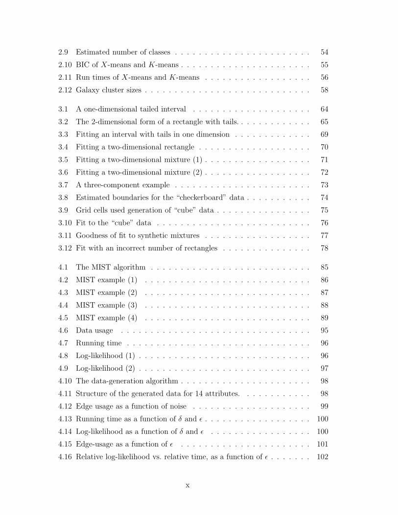
1.1 K-means example on a 2-D set (1) . . . . . . . . . . . . . . . . . . . 10




1.5 Domination with respect to a hyper-rectangle. . . . . . . . . . . . . . 17

1.6 Non-domination with respect to a hyper-rectangle. . . . . . . . . . . . 18

1.7 A recursive procedure to assign cluster memberships. . . . . . . . . . 19

1.8 Visualization of the hyper-rectangles owned by centroids . . . . . . . 20

1.9 Blacklisting of centroids . . . . . . . . . . . . . . . . . . . . . . . . . 22

1.10 Adding to the black list . . . . . . . . . . . . . . . . . . . . . . . . . 23

1.11 Comparative results on simulated data . . . . . . . . . . . . . . . . . 27

1.12 Effect of dimensionality on the blacklisting algorithm . . . . . . . . . 28

1.13 Effect of number of centroids on the blacklisting algorithm . . . . . . 29

1.14 Effect of number of points on the blacklisting algorithm . . . . . . . . 29

1.15 Approximated K-means . . . . . . . . . . . . . . . . . . . . . . . . . 30

1.16 Runtime of approximate clustering . . . . . . . . . . . . . . . . . . . 31

1.17 Distortion of approximate clustering . . . . . . . . . . . . . . . . . . 31

2.1 The X-means algorithm. . . . . . . . . . . . . . . . . . . . . . . . . . 42

2.2 X-means example (1) . . . . . . . . . . . . . . . . . . . . . . . . . . . 44

2.3 X-means example (2) . . . . . . . . . . . . . . . . . . . . . . . . . . . 44

2.4 X-means example (3) . . . . . . . . . . . . . . . . . . . . . . . . . . . 45

2.5 X-means example (4) . . . . . . . . . . . . . . . . . . . . . . . . . . . 45

2.6 X-means example (5) . . . . . . . . . . . . . . . . . . . . . . . . . . . 45

2.7 X-means overfitting . . . . . . . . . . . . . . . . . . . . . . . . . . . . 48

2.8 Distortion of X-means and K-means . . . . . . . . . . . . . . . . . . 52

ix

2.9 Estimated number of classes . . . . . . . . . . . . . . . . . . . . . . . 54

2.10 BIC of X-means and K-means . . . . . . . . . . . . . . . . . . . . . . 55

2.11 Run times of X-means and K-means . . . . . . . . . . . . . . . . . . 56

2.12 Galaxy cluster sizes . . . . . . . . . . . . . . . . . . . . . . . . . . . . 58

3.1 A one-dimensional tailed interval . . . . . . . . . . . . . . . . . . . . 64

3.2 The 2-dimensional form of a rectangle with tails. . . . . . . . . . . . . 65

3.3 Fitting an interval with tails in one dimension . . . . . . . . . . . . . 69

3.4 Fitting a two-dimensional rectangle . . . . . . . . . . . . . . . . . . . 70

3.5 Fitting a two-dimensional mixture (1) . . . . . . . . . . . . . . . . . . 71

3.6 Fitting a two-dimensional mixture (2) . . . . . . . . . . . . . . . . . . 72

3.7 A three-component example . . . . . . . . . . . . . . . . . . . . . . . 73

3.8 Estimated boundaries for the “checkerboard” data . . . . . . . . . . . 74

3.9 Grid cells used generation of “cube” data . . . . . . . . . . . . . . . . 75

3.10 Fit to the “cube” data . . . . . . . . . . . . . . . . . . . . . . . . . . 76

3.11 Goodness of fit to synthetic mixtures . . . . . . . . . . . . . . . . . . 77

3.12 Fit with an incorrect number of rectangles . . . . . . . . . . . . . . . 78

4.1 The MIST algorithm . . . . . . . . . . . . . . . . . . . . . . . . . . . 85

4.2 MIST example (1) . . . . . . . . . . . . . . . . . . . . . . . . . . . . 86

4.3 MIST example (2) . . . . . . . . . . . . . . . . . . . . . . . . . . . . 87

4.4 MIST example (3) . . . . . . . . . . . . . . . . . . . . . . . . . . . . 88

4.5 MIST example (4) . . . . . . . . . . . . . . . . . . . . . . . . . . . . 89

4.6 Data usage . . . . . . . . . . . . . . . . . . . . . . . . . . . . . . . . 95

4.7 Running time . . . . . . . . . . . . . . . . . . . . . . . . . . . . . . . 96

4.8 Log-likelihood (1) . . . . . . . . . . . . . . . . . . . . . . . . . . . . . 96

4.9 Log-likelihood (2) . . . . . . . . . . . . . . . . . . . . . . . . . . . . . 97

4.10 The data-generation algorithm . . . . . . . . . . . . . . . . . . . . . . 98

4.11 Structure of the generated data for 14 attributes. . . . . . . . . . . . 98

4.12 Edge usage as a function of noise . . . . . . . . . . . . . . . . . . . . 99

4.13 Running time as a function of δ and ε . . . . . . . . . . . . . . . . . . 100

4.14 Log-likelihood as a function of δ and ε . . . . . . . . . . . . . . . . . 100

4.15 Edge-usage as a function of ε . . . . . . . . . . . . . . . . . . . . . . 101

4.16 Relative log-likelihood vs. relative time, as a function of ε . . . . . . . 102

x

4.17 The Red Edge rule . . . . . . . . . . . . . . . . . . . . . . . . . . . . 104

4.18 The Blue Edge rule . . . . . . . . . . . . . . . . . . . . . . . . . . . . 104

4.19 Interval estimates . . . . . . . . . . . . . . . . . . . . . . . . . . . . . 106

5.1 Anomalies (Sloan data). . . . . . . . . . . . . . . . . . . . . . . . . . 110

5.2 The active learning loop . . . . . . . . . . . . . . . . . . . . . . . . . 111

5.3 Underlying data distribution for the example. . . . . . . . . . . . . . 113

5.4 Behavior of the lowlik method . . . . . . . . . . . . . . . . . . . . . . 115

5.5 Behavior of the ambig method . . . . . . . . . . . . . . . . . . . . . . 116

5.6 Behavior of the interleave method. . . . . . . . . . . . . . . . . . . . . 117

5.7 Different kinds of detected anomalies . . . . . . . . . . . . . . . . . . 119

5.8 Learning curves for simulated data . . . . . . . . . . . . . . . . . . . 121

5.9 Learning curves for the abalone set . . . . . . . . . . . . . . . . . . 122

5.10 Learning curves for the shuttle set . . . . . . . . . . . . . . . . . . 123

5.11 Learning curves for the kdd set . . . . . . . . . . . . . . . . . . . . . 123

5.12 Learning curves for the edsgc set . . . . . . . . . . . . . . . . . . . . 125

5.13 Learning curves for the sdss set . . . . . . . . . . . . . . . . . . . . . 125

5.14 Various objects spotted with the anomaly-hunting tool (Sloan data). . 127

6.1 The anomaly hunting application . . . . . . . . . . . . . . . . . . . . 130

6.2 The object information window . . . . . . . . . . . . . . . . . . . . . 131

6.3 The object explanation window . . . . . . . . . . . . . . . . . . . . . 132

6.4 The scatterplot window . . . . . . . . . . . . . . . . . . . . . . . . . . 133

6.5 The web window . . . . . . . . . . . . . . . . . . . . . . . . . . . . . 133

6.6 Ranks of anomalous objects . . . . . . . . . . . . . . . . . . . . . . . 135

xi

List of Tables

1.1 Comparative results on real data . . . . . . . . . . . . . . . . . . . . 25

1.2 Comparison against BIRCH . . . . . . . . . . . . . . . . . . . . . . . 26

2.1 Goodness of X-means fit for synthetic data . . . . . . . . . . . . . . . 53

2.2 Comparison of K-means, BIRCH, and X-means . . . . . . . . . . . . 54

3.1 Clusters for the “mpg” data . . . . . . . . . . . . . . . . . . . . . . . 78

3.2 Clusters for the “census” data . . . . . . . . . . . . . . . . . . . . . . 79

4.1 Results on real data . . . . . . . . . . . . . . . . . . . . . . . . . . . . 103

5.1 Properties of data sets . . . . . . . . . . . . . . . . . . . . . . . . . . 124

xiii

Introduction

Whenever we approach the so-called “data mining” problem, we realize it means

different things to different people. Scientists and analysts — the consumers of al-

gorithms and of data products — relate to the various tasks: pattern recognition,

structural organization, regression, anomaly finding, and so on. On top of that, we

as computer scientists — producers of algorithms and tools — break it down to its

building blocks: statistics, computational complexity, and knowledge management.

On first glance, it would seem this disparity has the potential for many false

expectations and impossible requirements. But the truth is that this very tension is

what advances research in the field. Here is how it typically happens. A scientist has

had access to some source of data, say experiments performed in his lab. Over time

he had accumulated a set of tools and techniques to analyze it. But recently, the

amount of data has become much larger. Possibly, new internet-based collaboration

points give him easy access to the results of other researchers’ work. Or perhaps new

machinery and methods are producing data orders of magnitude better — and faster

— than before. The Sloan Digital Sky Survey is a prime example of this. The goal is

to map, in detail, one-quarter of the entire sky. The estimated size of the catalog, due

to be completed in 2007, is 200 million objects, including images and spectroscopic

data. The database will then encompass 5 terabytes of catalog data, and 25 terabytes

of data overall.

The unforeseen outcome of such endeavors is that suddenly, the old tools become

useless. It might be because their theoretic complexity is poor and they blow up on

large inputs. Or because study of a single experiment is no longer interesting, when

one can potentially draw conclusions based on thousands of similar observations.

Or because the rate at which new results come exceeds the ability of an expert to

internalize it all, as the old summarization and visualization methods are inadequate.

This is the light under which the issues addressed in this work are best viewed.

Fundamentally, it deals with the difficulties of computer-literate and resourceful sci-

1

entists in a new world of abundant data. More concretely, we break this down into

several distinct components, each attempting to solve an admittedly small aspect of

the problem. The unifying element is the task - clustering. Historically, this is a task

that does not have a good definition that is both general and statistically rigorous.

We offer the intuitive definition of partitioning a given unlabeled data set into groups

such that elements in each group are somewhat more similar to each other (in some

unspecified measure of similarity) than they are to elements in other groups.1

Clustering can help in understanding the nature of a given data set in several

ways. First, the membership function by itself is meaningful, as it allows further

research involving just the part of the data that is of interest. For example, large-

scale cosmology simulations as well as recent astronomical surveys enable computation

of the correlation between the number of galaxies in a galaxy cluster, and the amount

of dark matter in it (“halo occupation distribution”). But before doing this, the

mapping from each galaxy to its owning cluster needs to be established.

A second potentially useful output is the number of clusters, if it is estimated by

the algorithm. This can serve as a characteristic of the data. Again we relate to

the universe example above for an example. By looking at the distribution of galaxy

cluster sizes, one can “profile” a given universe. This is potentially useful when

judging if a universe simulated from specific parameters is similar to the observed

universe (and also when analyzing the effect of changes to the simulation parameters).

Here, the number of clusters — typically in the order of thousands — clearly has to

be estimated from the data.

Third, the very description of the clusters defines subregions of the data space.

These descriptions can be used to achieve insights into the data. For example, if the

regions are convex, one can come up with unseen examples that would be included

in a given cluster. This ability can be useful for computer program verification tools

which aim to increase test-suite coverage.

Fourth, if the statistical model fitted to the data is a probability density estimator,

it can be used in a variety of related tasks. All the models described in this work

meet this criterion. Below we show how to use such models in an anomaly-hunting

task.

Note that we assume here that clusters form a flat hierarchy. This is somewhat

arbitrary, as a huge body of existing work deals with hierarchical clustering and fitting

of taxonomies. Much of that work is focused on information retrieval. Therefore, it

1Later we weaken this definition even further by considering the extension where each element

does not have to fully belong to just one class.

2

is sufficiently different from the kinds of data analyzed here to be outside the scope

of this work.

Clustering is used in a multitude of application areas. Some of them are:

• Large-scale cosmological simulations.

• Astronomical data analysis.

• Bioinformatics.

• Computer architecture.

• Musical information retrieval.

• Verification of computer programs.

• Natural language processing.

• Epidemiology.

• Highway traffic analysis.

Diverse as they are, in all of them we encounter similar phenomena. First, labels

for individual samples are rare or nonexistent (and too costly to obtain in the general

case). Second, the data is too voluminous to be entirely eyeballed by a human expert.

In fact, often it is too voluminous to even process mechanically quickly enough. To

illustrate the last point, consider an anomaly-hunting application which asks a human

expert for labels for a very small number of examples. Given those, it refines the

statistical model using the given examples and the full data set, and the cycle repeats.

Regardless of data set size, the computer run needs to finish quickly, or else the expert

would lose concentration.

Returning to the historical angle, most of the data analysts are already familiar

with some clustering method or another. The problem is that it is too slow on big

inputs. Generally, there are three approaches to address the speed issue:

1. Develop new algorithms and data-organization methods, such that the statis-

tical qualities of the data can be approximated quickly. Use the approximated

measures to generate output in the same form as the existing algorithms.

2. Develop exact and fast algorithms that output the exact same answer as the

original method. Enhance the data organization to support this kind of opera-

tion.

3

3. Develop near-exact algorithms using advanced data organization. Allow a user-

defined degree of error, or a probabilistic chance of making a mistake. Typically

those parameters will be very small.

The first example of the first approach is BIRCH (Zhang et al., 1995). It is an

approximate clusterer optimized for on-disk storage of large data sets. The clusters

are grown in a heuristic way. Very little can be said on the quality of the output

clusters, or about their difference from those obtained by some other method.

Another example of the first approach is sub-sampling. The idea is simple: ran-

domly select a small population from the input set and run the algorithm of choice

on it. A variant of this uses the results together with the original data set as if they

were created directly from the original set. For example, one might create clusters

based on a small sample, and then use the cluster centroids (or any other meaningful

property) to assign class membership to points in the original data.

Often, this approach is taken without much consideration of the statistical con-

sequences. Not surprisingly, they can be severe. For example, the 2-point correla-

tion function is used in cosmology to characterize sets of astronomical objects. It

is well-known that for the rich structure observed in our universe, straightforward

sub-sampling does not preserve the 2-point correlation function. And the same most

likely holds for other measures.

My conclusion is that there is merit in expending the effort to develop schemes

that can handle large data without affecting output quality. When this is too hard,

we would still like to bound the error in some way. This work aims to show that this

goal is achievable.

Below I describe how to accelerate several known algorithms, such that their

output can be used in exactly the same way as the output from the respective original

published versions. Empirical evaluation shows great speed-ups for many of them —

often two orders of magnitude faster than a straightforward implementation, measured

on actual data sets used by scientists. In one case the run time is even sub-linear in

the input size, and only depends on intrinsic properties of the data.

Chapter 1 looks at the familiar K-means algorithm and shows how it can be

accelerated by re-structuring the data. The output is exact (meaning the same as

it would be for a non-optimized algorithm). Chapter 2 uses the same fast data

structure to build a framework supporting estimation of the number of clusters K.

The framework exploits the data structure to accelerate the statistical test used for

model selection. It is also general in the sense that it allows a variety of statistical

4

measures for scoring and decision between different models. Chapter 3 takes a detour

to look at human comprehensibility. It proposes a new statistical model which lends

itself to succinct descriptions of clusters. This description can be read by a domain

expert with no knowledge of machine learning, and its predicates can be interpreted

directly in the application domain. In Chapter 4 we return to dealing with a well-

known statistical algorithm. This time we focus on dependency trees as grown by

popular the Chow-Liu algorithm and propose a “probably approximately correct”

algorithm to fit them. It can decide to consider just a subset of the data for certain

computations, if this can be justified by data data already scanned. In practice,

this typically happens very quickly, resulting in large speed-ups. In Chapter 5 we

consider the task of anomaly-hunting in large noisy sets, where the classes containing

the anomalies are extremely rare. For help, we consult an “oracle” for labels for a

very small number of examples, which naturally touches on active learning. This

work uses the fast dependency tree learner, however it is not dependent on it and can

use other models as components. Finally, in Chapter 6 I describe a visual tool based

on these ideas, which enables an expert to interact with the data and find anomalies

quickly.

5

Chapter 1

Fast K-means

Modern cosmology relies on simulation data to validate or disprove theories. For

example, a universe of several million objects would be created and evolved over

time. The simulation data is then available for large-scale analysis. Historically, such

tasks — including clustering — were performed on huge data sets by taking a random

sub-sample and applying the technique on hand to the smaller set such that it finishes

in a reasonable amount of time. Afterwards the results (say, cluster definitions) are

somehow projected back to the original data space.

This kind of approach is impractical for cosmology. The fundamental reason is

that the rich structure of the universe cannot be easily down-sampled. For example,

the 2-point correlation function is used as a succinct summary of spatial data. It is

known that random sampling fails to preserve the properties of the 2-point function.

Therefore any astrophysicist would be justified to suspect output from a process that

starts by reducing the data in such a destructive way. The right way is to devise ways

to process large amounts of data natively.

I present new algorithms for the K-means clustering problem. While being ex-

tremely fast, they do not make any kind of approximation. Empirical results show a

speedup factor of up to 170 on real astrophysical data, and superiority over the naive

algorithm on simulated data. My algorithms scale sub-linearly with respect to the

number of points and linearly with the number of clusters. This allows for clustering

with tens of thousands of centroids and millions of points using commodity hardware.

7

1.1 Introduction

Consider a dataset with R records, each having M attributes. Given a constant k, the

clustering problem is to partition the data into k subsets such that each subset behaves

“well” under some measure. For example, we might want to minimize the squared

Euclidean distances between points in any subset and their center of mass. The

K-means algorithm for clustering finds a local optimum of this measure by keeping

track of centroids of the subsets, and issuing a large number of nearest-neighbor

queries (Gersho & Gray, 1992).

A kd-tree is a data structure for storing a finite set of points from a finite-

dimensional space (Bentley, 1980). Its usage in very fast EM-based Mixture Model

Clustering was shown by Moore (1998). The need for such a fast algorithm arises

when conducting massive-scale model selection, and in datasets with a large number

of attributes and records. An extreme example is the data which is gathered in the

Sloan Digital Sky Survey (SDSS) (SDSS, 1998), where M is about 500 and R is in

the tens of millions.

In this chapter, I show that kd-trees can be used to reduce the number of nearest-

neighbor queries in K-means by using the fact that their nodes can represent a large

number of points. I am frequently able to prove for certain nodes of the kd-tree

statements of the form “any point associated with this node must have X as its

nearest neighbor” for some centroid X. This, together with a set of statistics stored

in the kd-nodes, allows for great reduction in the number of arithmetic operations

needed to update the centroids of the clusters.

I have implemented my algorithms and tested their behavior with respect to vari-

ations in the number of points, dimensions, and centroids, as measured on synthetic

data. I also present results of tests on preliminary SDSS data.

The remainder of this chapter is organized as follows. In Section 1.2 I introduce

notation and describe the original K-means algorithm. In Section 1.3 I present my

algorithms with proofs of correctness. Section 1.4 elaborates on the finer points of the

implementation. Section 1.5 discusses results of experiments on real and simulated

data. Section 1.6 discusses related work, and Section 1.7 concludes and suggests ideas

for further work.

8

1.2 Definitions

Throughout this chapter, I denote the number of records by R, the number of dimen-

sions by M and the number of centroids by k.

I first describe the naive K-means algorithm for producing a clustering of the

points in the input into k clusters. It is the best known of all clustering algorithms,

and literally hundreds of papers about its theory and deployment have appeared

in the statistics literature in the last 20 years (Duda & Hart, 1973; Bishop, 1995).

It partitions the data points into k subsets such that all points in a given subset

“belong” to some centroid. The algorithm keeps track of the centroids of the subsets,

and proceeds in iterations. We denote the set of centroids after the i-th iteration

by C(i). Before the first iteration the centroids are initialized to arbitrary locations.

The algorithm terminates when C(i) and C(i−1) are identical. In each iteration, the

following is performed:

1. For each point x, find the centroid in C(i) which is closest to

x. Associate x with this centroid.

2. Compute C(i+1) by taking, for each centroid, the center of mass

of points associated with this centroid.

Figures 1.1, 1.2 and 1.3 give a graphical demonstration of K-means when run on

an example dataset.

My algorithms involve modification of just the code within one iteration. I there-

fore analyze the cost of a single iteration. The naive K-means described above per-

forms a nearest-neighbor query for each of the R points. During such a query the

distances in M -space to k centroids are calculated. Therefore the cost is O(kMR).

One fundamental tool I will use to tackle the problem is the kd-tree data-structure.

I outline its relevant properties, and from this point on will assume that a kd-tree for

the input points exists. Further details about kd-trees can be found in Moore (1991).

I will use a specialized version of kd-trees called mrkd-trees, for “multi-resolution

kd-trees” (Deng & Moore, 1995). The properties of kd-trees relevant to this work are:

• They are binary trees.

• Each node contains information about all points contained in a hyper-rectangle

h. The hyper-rectangle is stored at the node as two M -length boundary vectors

9

(a) (b)

(c) (d)

Figure 1.1: A 2-D set of 8000 points, drawn from a mixture of 5 spherical Gaussians

(a). The 5 initial centroids (b). The partition induced by the centroids (c). For each

centroid, the center of mass of points it owns is computed and connected to its current

location with a line (d). Note how black and red share the left-hand cluster, and will

“race” towards it. (Continued).

10

(a) (b)

(c) (d)

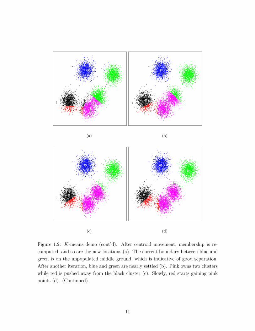
Figure 1.2: K-means demo (cont’d). After centroid movement, membership is re-

computed, and so are the new locations (a). The current boundary between blue and

green is on the unpopulated middle ground, which is indicative of good separation.

After another iteration, blue and green are nearly settled (b). Pink owns two clusters

while red is pushed away from the black cluster (c). Slowly, red starts gaining pink

points (d). (Continued).

11

(a) (b)

(c) (d)

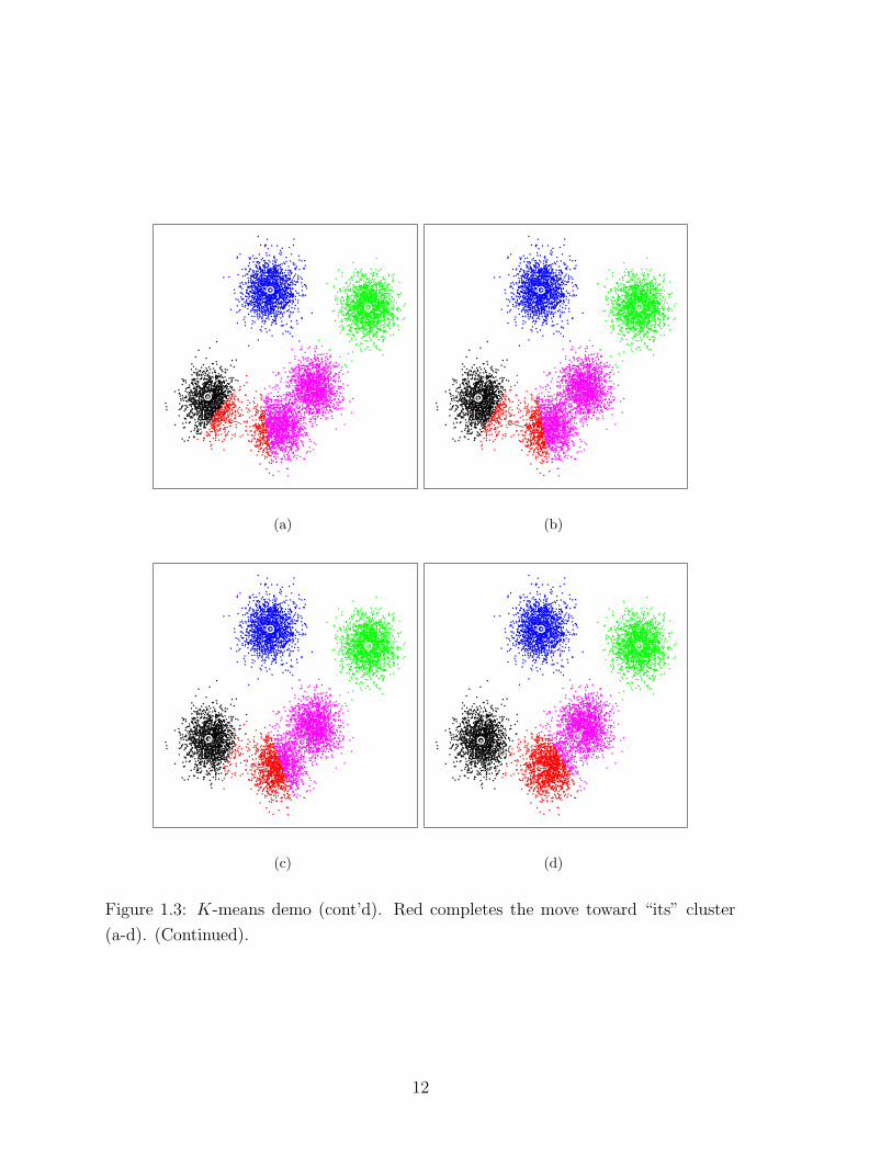
Figure 1.3: K-means demo (cont’d). Red completes the move toward “its” cluster

(a-d). (Continued).

12

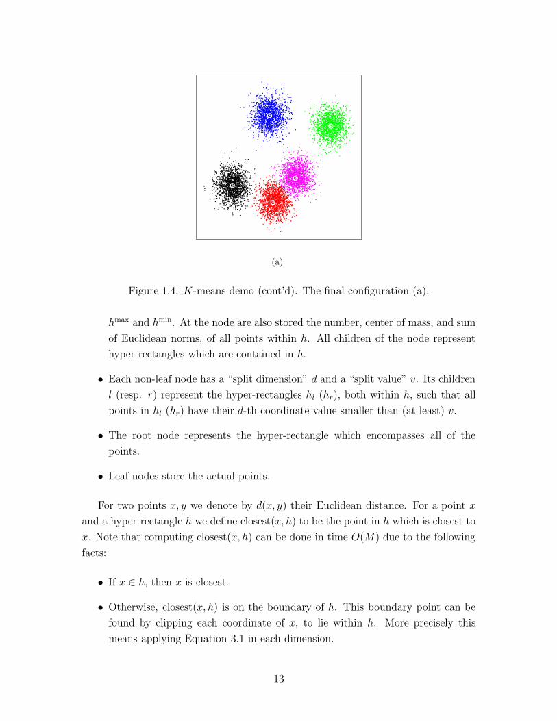
(a)

Figure 1.4: K-means demo (cont’d). The final configuration (a).

hmax and hmin. At the node are also stored the number, center of mass, and sum

of Euclidean norms, of all points within h. All children of the node represent

hyper-rectangles which are contained in h.

• Each non-leaf node has a “split dimension” d and a “split value” v. Its children

l (resp. r) represent the hyper-rectangles hl (hr), both within h, such that all

points in hl (hr) have their d-th coordinate value smaller than (at least) v.

• The root node represents the hyper-rectangle which encompasses all of the

points.

• Leaf nodes store the actual points.

For two points x, y we denote by d(x, y) their Euclidean distance. For a point x

and a hyper-rectangle h we define closest(x, h) to be the point in h which is closest to

x. Note that computing closest(x, h) can be done in time O(M) due to the following

facts:

• If x ∈ h, then x is closest.

• Otherwise, closest(x, h) is on the boundary of h. This boundary point can be

found by clipping each coordinate of x, to lie within h. More precisely this

means applying Equation 3.1 in each dimension.

13

We define the distance d(x, h) between a point x and a hyper-rectangle h to be

d(x, closest(x, h)). For a hyper-rectangle h we denote by width(h) the vector hmax −hmin.

Given a clustering φ, we denote by φ(x) the centroid this clustering associates

with an arbitrary point x (so for K-means, φ(x) is simply the centroid closest to x).

We then define a measure of quality for φ:

distortionφ =1

R·∑

x

d2(x, φ(x)) , (1.1)

where R is the total number of points and x ranges over all input points.

1.3 Algorithms

My algorithms exploit the fact that instead of updating the centroids point by point,

a more efficient approach is to update in bulk. This can be done using the known

centers of mass and size of groups of points. Specifically, we look at the center-of-mass

update from Algorithm 1.2:

C(i+1)j =

∑

x∈Q ~x

|Q| (1.2)

where j indexes some centroid and Q denotes all the points “belonging” to this

centroid (I omit the iteration and centroid indices from Q for clarity). Now consider

some partition of Q, that is a set {Qp} such that:

⋃

p

Qp = Q

Qp ∩Qj = ∅ ∀i 6= j .

It is obviously true that

C(i+1)j =

∑

p

∑

x∈Qp~x

∑

p |Qp|. (1.3)

Naturally, the sets Qp will correspond to nodes in the kd-tree. Recall that for

those we compute the sums and counts of the included points in advance and store

them with the node. Hence the inner summation above reduces to a simple look-up.

The optimization above is not limited to vector sums. Any kind of additive quan-

tity can be computed in the same way. The count is another such measure (the value

14

summed for each point being one). I use it also to compute the distortion. The key

equality for this is:

d2(x, y) = (~x− ~y) · (~x− ~y)

= ||x||2 − 2x · y + ||y||2 .

In the distortion computation (see Equation 1.1), x ranges over points and y = φ(x)

is the owning centroid. So for a particular subset Qp such that all points in it belong

to the same centroid, y is a constant and can be factored out. Additionally I pre-

compute and store∑ ||x||2 for each kd-node similarly to the vector sums. I also use

a similar technique in obtaining the sets of points which belong to each centroid (as

needed by some statistics). For other obtainable statistics see Zhang et al. (1995).

The challenge now shifts to making sure that all of the points in a given hyper-

rectangle indeed “belong” to a specific centroid before adding their statistics to it.

Below I lay out a framework to support these kinds of assertions. We begin with the

notion of an owner.

Definition 1 Given a set of centroids C and a hyper-rectangle h, we define by

ownerC(h) a centroid c ∈ C such that any point in h is closer to c than to any

other centroid in C, if such a centroid exists.

We will omit the subscript C where it is clear from the context. The rest of this

section discusses owners and efficient ways to find them. We start by analyzing a

property of owners, which, by listing those centroids which do not have it, will help

us eliminate non-owners from the set of possibilities. Note that ownerC(h) is not

always defined. For example, when two centroids are both inside a rectangle, then

there exists no unique owner for this rectangle. Therefore the precondition of the

following theorem is that there exists a unique owner. The algorithmic consequence

is that my method will not always find an owner, and will sometimes be forced to

descend the kd-tree, thereby splitting the hyper-rectangle in hope to find an owner for

the smaller hyper-rectangle. I return to this scenario later. For now I give a necessary

condition for an owner.

Theorem 2 Let C be a set of centroids, and let h be a hyper-rectangle. Let c ∈ C be

ownerC(h). Then:

d(c, h) = minc′∈C

d(c′, h) .

15

Proof: Assume, for the sake of contradiction, that c 6= arg minc′∈C d(c′, h) ≡ c∗.

Then there exists a point in h (namely closest(c∗, h)) which is closer to c′ than to c.

This is in contradiction to the definition of c as owner(h). �

We distinguish between “shortest” and “minimal” distance. We define shortest

to be the optimized measure only when it is unique. In contrast, the definition of

minimal always holds and includes any element which attains the minimum. So there

can be multiple minimal elements. But only if there is a single such element, then

we say it attains the shortest distance. In these terms, we can say that when looking

for owner(h), we should only consider centroids with shortest distance d(c, h). For

example, suppose that two (or more) centroids share the minimal distance to h. Then

neither can claim to be an owner. This situation arises more often than one would

initially expect. In particular, all the centroids inside a given kd-node have distance

zero to the node.

Theorem 2 narrows down the number of possible owners to either one (if there ex-

ists a shortest distance centroid) or zero (otherwise). In the latter case, my algorithm

will proceed by splitting the hyper-rectangle. In the former case, all we have is a nec-

essary condition, but it is not sufficient. Consequently we still have to check if this

candidate is an owner of the hyper-rectangle in question. As will become clear from

the following discussion, this will not always be the case. Let us begin by defining a

restricted form of ownership, where just two centroids are involved.

Definition 3 Given a hyper-rectangle h, and two centroids c1 and c2 such that d(c1, h) <

d(c2, h), we say that c1 dominates c2 with respect to h if every point in h is closer to

c1 than it is to c2.

Observe that if some c ∈ C dominates all other centroids with respect to some h,

then c = owner(h). A possible (albeit inefficient) way of finding owner(h) if one exists

would be to scan all possible pairs of centroids. However, using theorem 2, we can

reduce the number of pairs to scan since c1 is fixed. To prove this approach feasible

we need to show that the domination decision problem can be solved efficiently.

Lemma 4 Given two centroids c1, c2, and a hyper-rectangle h such that d(c1, h) <

d(c2, h), the decision problem “does c1 dominate c2 with respect to h?” can be answered

in O(M) time.

Proof: Observe the decision line L12 composed of all points which are equidistant

to c1 and c2 (see Figures 1.5 and 1.6). If c1 and h are both fully contained in one half-

16

c1

L12

h

p12

c2

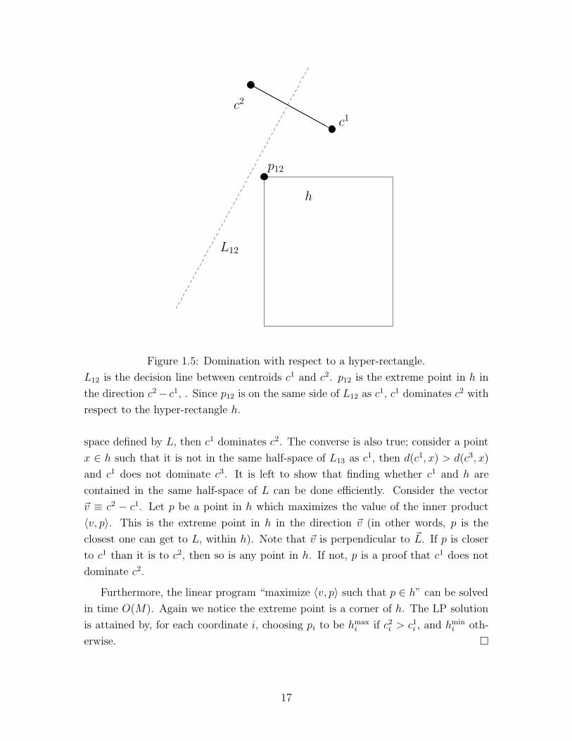
Figure 1.5: Domination with respect to a hyper-rectangle.

L12 is the decision line between centroids c1 and c2. p12 is the extreme point in h in

the direction c2− c1, . Since p12 is on the same side of L12 as c1, c1 dominates c2 with

respect to the hyper-rectangle h.

space defined by L, then c1 dominates c2. The converse is also true; consider a point

x ∈ h such that it is not in the same half-space of L13 as c1, then d(c1, x) > d(c3, x)

and c1 does not dominate c3. It is left to show that finding whether c1 and h are

contained in the same half-space of L can be done efficiently. Consider the vector

~v ≡ c2 − c1. Let p be a point in h which maximizes the value of the inner product

〈v, p〉. This is the extreme point in h in the direction ~v (in other words, p is the

closest one can get to L, within h). Note that ~v is perpendicular to ~L. If p is closer

to c1 than it is to c2, then so is any point in h. If not, p is a proof that c1 does not

dominate c2.

Furthermore, the linear program “maximize 〈v, p〉 such that p ∈ h” can be solved

in time O(M). Again we notice the extreme point is a corner of h. The LP solution

is attained by, for each coordinate i, choosing pi to be hmaxi if c2

i > c1i , and hmin

i oth-

erwise. �

17

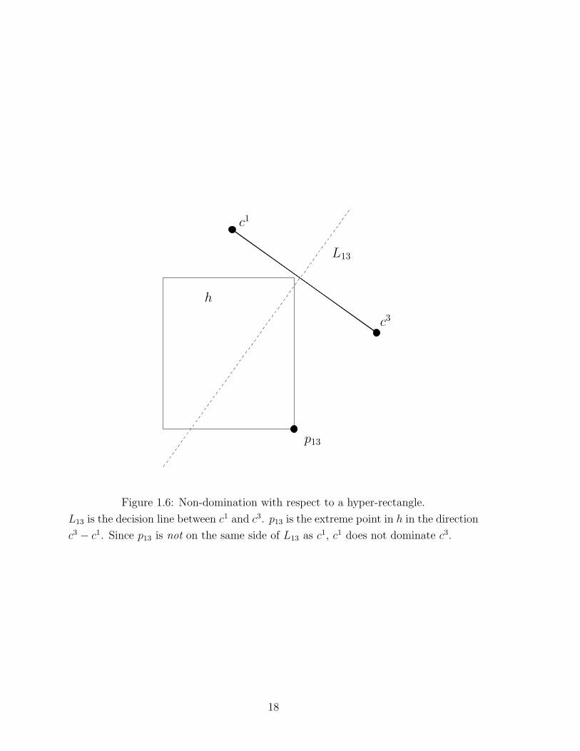
c3

p13

h

c1

L13

Figure 1.6: Non-domination with respect to a hyper-rectangle.

L13 is the decision line between c1 and c3. p13 is the extreme point in h in the direction

c3 − c1. Since p13 is not on the same side of L13 as c1, c1 does not dominate c3.

18

Update(h, C):

1. If h is a leaf:

(a) For each data point in h, find the closest centroid to it

and update the counters for that centroid.

(b) Return.

2. Compute d(c, h) for all centroids c. If there exists one centroid

c with shortest distance:

If for all other centroids c′, c dominates c′ with respect to

h (so we have established c = owner(h)):

(a) Update counters for c using the data in h.

(b) Return.

3. Call Update(hl, C).

4. Call Update(hr, C).

Figure 1.7: A recursive procedure to assign cluster memberships.

1.3.1 The Simple Algorithm

I now describe a procedure to update the centroids in C (i). It will take into consid-

eration an additional parameter, a hyper-rectangle h such that all points in h affect

the new centroids. The procedure is recursive, with the initial value of h being the

universal hyper-rectangle with all of the input points in it. If the procedure can find

owner(h), it updates its counters using the center of mass and number of points which

are stored in the kd-node corresponding to h (I will frequently interchange h with the

corresponding kd-node). Otherwise, it splits h by recursively calling itself with the

children of h. Pseudo-code for this procedure is in Figure 1.7. The correctness follows

from the discussion above.

We would not expect my Update procedure to prune in the case that h is the

universal set of all input points (since all centroids are contained in it, and therefore

no shortest-distance centroid exists). We also notice that if the hyper-rectangles were

split again and again so that the procedure is dealing just with leaves, this method

would be identical to the original K-means. In fact, this implementation will be

19

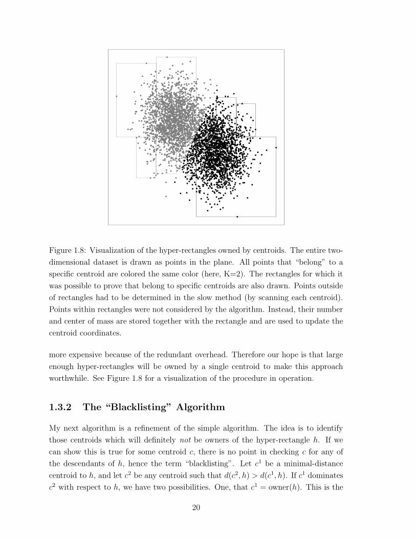
Figure 1.8: Visualization of the hyper-rectangles owned by centroids. The entire two-

dimensional dataset is drawn as points in the plane. All points that “belong” to a

specific centroid are colored the same color (here, K=2). The rectangles for which it

was possible to prove that belong to specific centroids are also drawn. Points outside

of rectangles had to be determined in the slow method (by scanning each centroid).

Points within rectangles were not considered by the algorithm. Instead, their number

and center of mass are stored together with the rectangle and are used to update the

centroid coordinates.

more expensive because of the redundant overhead. Therefore our hope is that large

enough hyper-rectangles will be owned by a single centroid to make this approach

worthwhile. See Figure 1.8 for a visualization of the procedure in operation.

1.3.2 The “Blacklisting” Algorithm

My next algorithm is a refinement of the simple algorithm. The idea is to identify

those centroids which will definitely not be owners of the hyper-rectangle h. If we

can show this is true for some centroid c, there is no point in checking c for any of

the descendants of h, hence the term “blacklisting”. Let c1 be a minimal-distance

centroid to h, and let c2 be any centroid such that d(c2, h) > d(c1, h). If c1 dominates

c2 with respect to h, we have two possibilities. One, that c1 = owner(h). This is the

20

good case since we do not need any more computation. The other option is that we

have not identified an owner for this node. The slow algorithm would have given up

at this point and restarted a computation for the children of h. For the blacklisting

version, we make use of the following.

Lemma 5 Given two centroids c1 and c2 such that c1 dominates c2 with respect to a

hyper-rectangle h, c1 also dominates c2 with respect to any h′ ⊆ h.

Proof: Immediate from Definition 3. �

Theorem 6 Given two centroids c1 and c2 such that c1 dominates c2 with respect to a

kd-node h, it is not necessary to consider c2 for the purpose of determining ownerC(h′)

for any descendant of h.

Proof: Recall that each kd-node fully contains any of its descendants. Let h′ be

a descendant of h. From Lemma 5 we get that c1 dominates c2 with respect to h′.

Therefore c2 cannot be ownerC(h′). �

The blacklisting version makes use of Theorem 6 by removing c2 from the list of

candidates. The list of prospective owners thus shrinks until it reaches a size of 1. At

this point we declare the only remaining centroid the owner of the current node h.

Again, we hope this happens before h is a leaf node, to maximize the savings. But

even if it does not, we still save work by not considering any centroid in the blacklist.

Figure 1.9 shows how the blacklist evolves during a traversal of an example kd-tree.

For a typical run with 30000 points and 100 centroids, I measured that blacklisting

algorithm calculates distances from points to centroids about 270000 times in each

iteration. This, plus the overhead, is to be compared with the 3 million distances the

naive algorithm has to calculate.

1.4 Implementation

The implementation uses the following architecture for flexibility. The tree-traversal

code is generic, and provides hooks for the following actions and predicates:

• Action to perform when discovering a point belongs to some centroid.

21

f

d

g

a

b c

e

{1,2,3,4,5,6}

{1,2,5,6}

{1,2,3,4,5,6}

{2}

{1,2,3,4,5,6}

{1,2,5,6}{1,2,5,6}

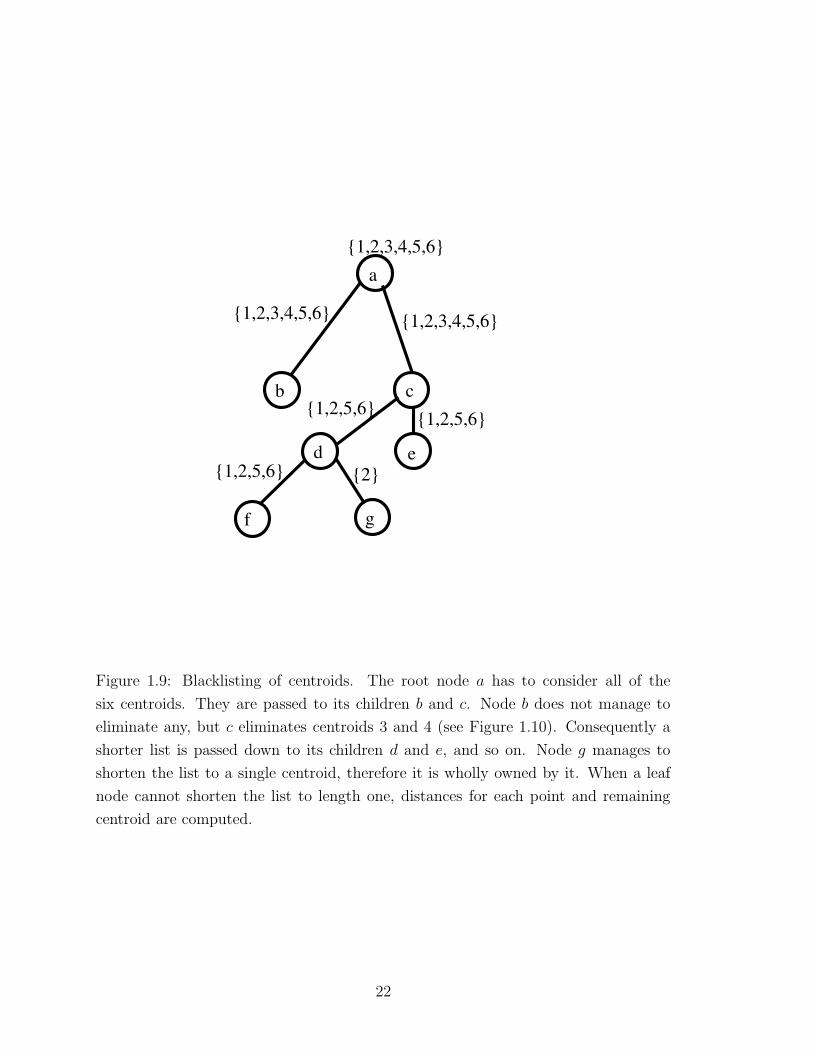
Figure 1.9: Blacklisting of centroids. The root node a has to consider all of the

six centroids. They are passed to its children b and c. Node b does not manage to

eliminate any, but c eliminates centroids 3 and 4 (see Figure 1.10). Consequently a

shorter list is passed down to its children d and e, and so on. Node g manages to

shorten the list to a single centroid, therefore it is wholly owned by it. When a leaf

node cannot shorten the list to length one, distances for each point and remaining

centroid are computed.

22

C1

C3

C2

C5

C6

C4

Figure 1.10: Adding to the black list. An example configuration consistent with the

blacklisting for node c in Figure 1.9. Centroid c5 is closet to the kd-node in question.

The two boundary lines prove that it dominates c3 and c4 respectively with respect

to the node. Therefore c3 and c4 can be eliminated from future searches.

• Action to perform when discovering a whole kd-node belongs to some centroid.

• Predicate for pruning the search at this node and not traversing its descendants.

This framework proved useful in supporting many kinds of operations on the kd-trees.

Among them:

• Maintaining vector sums and counts for center-of-mass calculations.

• Maintaining second moment sums for distortion calculations.

• Output of membership lists.

• Localized K-means runs (see Chapter 2).

Another optimization relates to the locality of changes in centroid locations. Of-

ten, some regions of the data will stabilize faster than others, in the sense that cen-

troids in them will reach their final locations much sooner. For example, see how in

Figure 1.3 (a–d), the top two centroids do not move at all while the bottom centroids

still exchange data points. The opportunity here is to save computation by re-using

membership information from previous iterations.

The way to achieve this is by storing the results of computations for future use.

This is done at the kd-node level. For example, we might record that in a given

node, there were two specific centroids competing for the points, as well the total

23

contribution to the accumulated moments due to the node for each of the centroids.

This is done during the traversal by considering the values for the accumulators before

and after the node is processed. The difference is stored in the node, along with the

list of competitors. If, during a subsequent traversal, the competitor list is the same

as it is in the cache for this node, the stored statistics are added to the running

accumulators instead of traversing the node. There is a small limit to the length of

the competitor list, to save memory and to ensure that caching is done only at local

regions.

A pre-assumption of this caching scheme is that centroid identifiers are indicative

of their location. Assume that we cache the effect some node would have on centroids

numbers 3 and 5. Before the next iteration, one or both of them moves slightly. On

the next iteration, we could still have 3 and 5 as the only competitors for the node.

However matching on the identifiers 3 and 5 and using old information would be

wrong, since the new locations can shift the balance between them considerably.

We therefore use a write-once data structure to store centroids. It supports insert

and delete operations, but not update. Whenever a centroid moves, we delete its old

identifier and insert a new item. This way, a match in identifiers guarantees both

elements are indeed equal.

1.5 Experimental Results

I have conducted experiments on both real and randomly-generated data. The real

data is preliminary SDSS data with some 400,000 celestial objects. The synthetic

data covers a wide range of parameters that might affect the performance of the

algorithms. Some of the measures are comparative, and measure the performance of

my algorithms against the naive algorithm, and against the BIRCH (Zhang et al.,

1995) algorithm. Others simply test the behavior of my fast algorithm on different

inputs.

The real data is a two-dimensional data set, containing the X and Y coordinates

of objects observed by a telescope. There were 433,208 such objects in my data

set. Note that “clustering” in this domain has a well-known astrophysical meaning

of clusters of galaxies, etc. Such clustering, however, is somewhat insignificant in a

two-dimensional domain since the physical placement of the objects is in 3-space. The

results are shown in Table 1.1. The main conclusion is that the blacklisting algorithm

executes 25 to 176 times faster than the naive algorithm, depending on the number

of points.

24

points blacklisting naive speedup

50000 2.02 52.22 25.9

100000 2.16 134.82 62.3

200000 2.97 223.84 75.3

300000 1.87 328.80 176.3

433208 3.41 465.24 136.6

Table 1.1: Comparative results on real data. Run-times of the naive and blacklisting

algorithm, in seconds per iteration. Run-times of the naive algorithms also shown

as their ratio to the running time of the blacklisting algorithm, and as a function of

number of points. Results were obtained on random samples from the 2-D “petro”

file using 5000 centroids.

In addition, I have conducted experiments with the BIRCH algorithm (Zhang

et al., 1995). It is similar to my approach in that it keeps a tree of nodes representing

sets of data points, together with sufficient statistics. The experiment was conducted

as follows. I let BIRCH run through phases 1 through 4 and terminate, measuring

the total run-time. This is normal mode of operation for BIRCH. Then I ran my

K-means algorithm for as many iterations as possible, given this time limit. I then

measured the distortion of the clustering output by both algorithms. The results are

in Table 1.2. In seven experiments out of ten, the blacklisting algorithm produced

better (i.e., lower distortion) results. These experiments include randomly generated

data files originally used as a test-case in Zhang et al. (1995), random data files

generated by me, and real data.

The synthetic experiments were conducted in the following manner. First, a data

set was generated using 72 randomly-selected points (class centers). For each data

point, a class was first selected at random. Then, the point coordinates were cho-

sen independently under a Gaussian distribution with mean at the class center, and

deviation σ equal to the number of dimensions times 0.025. One data set contained

200, 000 points drawn this way. The naive, hyperplane-based, and blacklisting al-

gorithms were run on this data set and measured for speed. Notice that all three

algorithms generate exactly the same set of centroids in each iteration, so the number

of iterations for all three of them is identical, given the data set. This experiment

was repeated 30 times and averages were taken. The number of dimensions varied

from 2 to 16. The number of clusters each algorithm was requested to find was 72.

The results are shown in Figure 1.11. The main observation is that for this data, the

blacklisting algorithm is faster than the naive approach in 2 to 6 dimensions, with

speedup of up to 27-fold in two dimensions. In higher dimensions it is slower. My

25

dataset form points K blacklisting BIRCH BIRCH,

distortion distortion relative

1 grid 100000 100 1.85 1.76 0.95

2 sine 100000 100 2.44 1.99 0.82

3 random 100000 100 6.98 8.98 1.29

4 random 200000 250 7.94e-4 9.78e-4 1.23

5 random 200000 250 8.03e-4 1.01e-3 1.25

6 random 200000 250 7.91e-4 1.00e-3 1.27

7 real 100000 1000 3.59e-2 3.17e-2 0.88

8 real 200000 1000 3.40e-2 3.51e-2 1.03

9 real 300000 1000 3.73e-2 4.19e-2 1.12

10 real 433208 1000 3.37e-2 4.08e-2 1.21

Table 1.2: Comparison against BIRCH. The distortion for the blacklisting and BIRCH

algorithms, given equal run-time, is shown. Six of the datasets are simulated and 4

are real (“petro” data from SDSS). Datasets 1–3 are as published in Zhang et al.

(1995). Datasets 4–6 were generated randomly as described. For generated datasets,

the number of classes in the original distribution is also the number of centroids

reported to both algorithms. The last column shows the BIRCH output distortion

divided by the blacklisting output distortion (i.e., if it is larger than 1 than BIRCH

is performing worse).

26

0

0.2

0.4

0.6

0.8

1

1.2

1.4

1.6

1.8

2

2.2

2 3 4 5 6 7 8

time

dimensions

200000 points, 72 classes

hplaneslow

blacklist

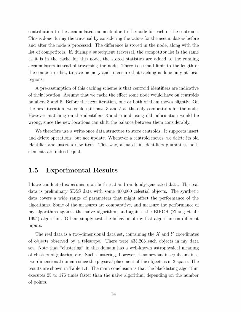
Figure 1.11: Comparative results on simulated data. Running time, in seconds, is

shown as the number of dimensions varies. Each line stands for a different algorithm:

the naive algorithm (“slow”), my simple algorithm (“hplane”), and the blacklisting

algorithm (“black”).

simple algorithm is slower, but still faster than the naive approach. In 8 or more

dimensions blacklisting is slowest, due to overhead, and naive and simple are approx-

imately the same (results not shown). Note this graph can be “stretched” so that

blacklisting is still faster in higher dimensions, by increasing the number of points.

Another interesting experiment to perform is to measure the sensitivity of my

algorithms to changes in the number of points, centroids, and dimensions. It is

known, by direct analysis, that the naive algorithm has linear dependence on these.

It is also known that kd-trees tend to suffer from high dimensionality. In fact, I have

just established that in the comparison to the naive algorithm. See Moore (1991) as

well. To this end, another set of experiments was performed. The experiments used

generated data as described earlier (only with 30000 points). But, only the blacklisting

algorithm was used to cluster the data and the running time was measured. In this

experiment set, the number of dimensions varied from 1 to 8 and the number of

centroids the program was requested to generate varied from 10 to 80 in steps of

10. The results are shown in Figure 1.12. The number of dimensions seems to have

a super-linear effect on the blacklisting algorithm. This worsens as the number of

centroids increases.

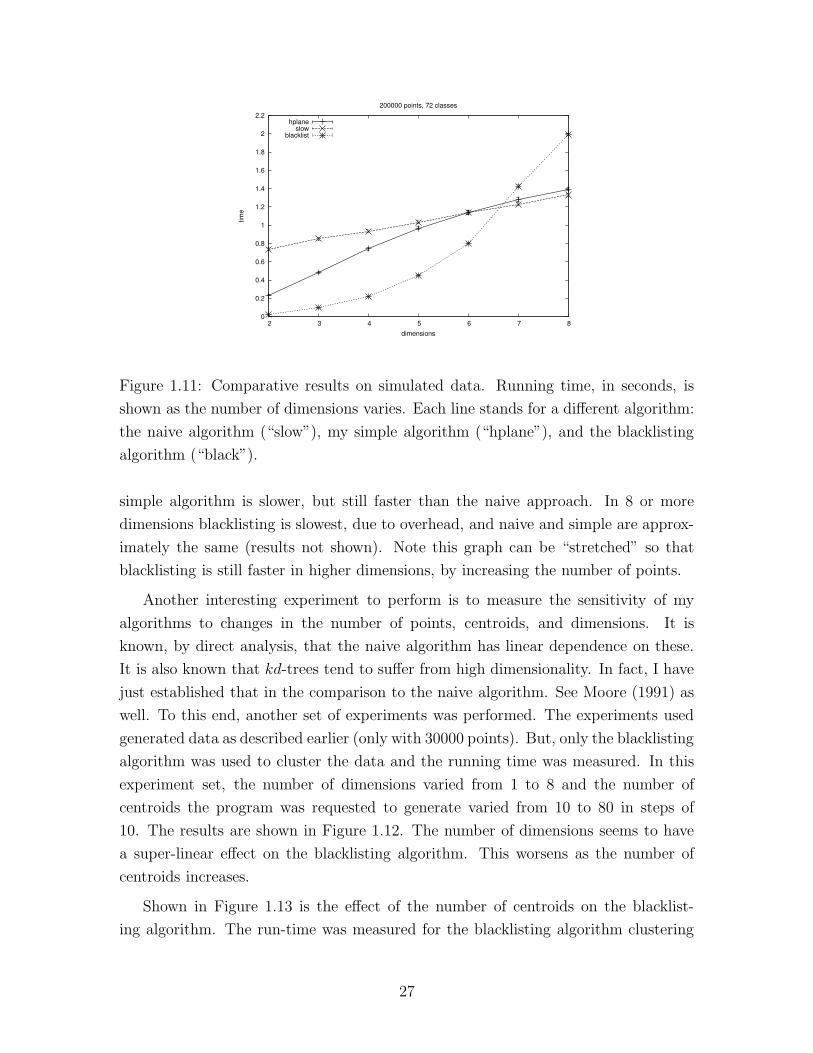
Shown in Figure 1.13 is the effect of the number of centroids on the blacklist-

ing algorithm. The run-time was measured for the blacklisting algorithm clustering

27

0

0.2

0.4

0.6

0.8

1

1.2

1 2 3 4 5 6 7 8

time

#dimensions

plot for: 30000 points

"nclasses=10""nclasses=20""nclasses=30""nclasses=40""nclasses=50""nclasses=60""nclasses=70""nclasses=80"

Figure 1.12: Effect of dimensionality on the blacklisting algorithm. Running time, in

seconds per iteration, is shown as the number of dimensions varies. Each line shows

results for a different number of classes (centroids).

random subsets of varying size from the astronomical data, with 50, 500, and 5000

centroids. We see that the number of centroids has a linear effect on the algorithm.

This result was confirmed on simulated data (data not shown).

In Figure 1.14 the same results are shown, now using the number of points for the

X axis. We see a very small increase in run-time as the number of points increases.

1.5.1 Approximate Clustering

Another way to accelerate clustering is to prune the search when only small error is

likely to be incurred. See Figure 1.15. We do this by not descending down the kd-tree

when a “small-error” criterion holds for a specific node. We then assume that the

points of this node (and its hyper-rectangle h) are divided evenly among all current

competitors (meaning all those centroid not currently blacklisted). For each such

competing centroid c, we update its location as if the relative number of points are

all located at closest(c, h). Our pruning criterion is:

n ·M∑

j=1

(

width(h)j

width(U)j

)2

≤ di

where n denotes the number of points in h, U is the “universal” hyper-rectangle,

i is the iteration number, and d is a constant, typically set to 0.8. The idea is to

28

0

1

2

3

4

5

6

7

0 1000 2000 3000 4000 5000 6000 7000 8000 9000 10000

time

# classes

’gpetro’ astrophysical data

"npoints=10000""npoints=50000"

"npoints=100000""npoints=200000""npoints=300000""npoints=433208"

Figure 1.13: Effect of number of centroids on the blacklisting algorithm. Running

time, in seconds per iteration, is shown as the number of classes (centroids) varies.

Each line shows results for a different number of random points from the original file.

0

0.1

0.2

0.3

0.4

0.5

0.6

0 50000 100000 150000 200000 250000 300000 350000 400000 450000

time

#points

’petro’ astrophysical data

"nclasses=5""nclasses=50"

"nclasses=500"

Figure 1.14: Effect of number of points on the blacklisting algorithm. Running time,

in seconds per iteration, is shown as the number of points varies. Each line shows

results for a different number of classes.

29

Figure 1.15: Illustration of approximated K-means. Two centroids are shown in

gray. Also shown is the decision line between them. A kd-node intersects the line and

contains very few points. The overall effect of node on the centroid locations can be

approximated without examining individual points.

(heuristically) bound the error contribution from any given node. The exponent i

dictates a “cooling schedule” where at the first few iterations it is allowed to make

bigger mistakes than later on. So at the beginning the clustering is approximate and

fast. But in subsequent iterations it becomes more and more accurate. Note that

in later iterations we have a better chance of hitting cached nodes, so this does not

necessarily imply a slowdown.

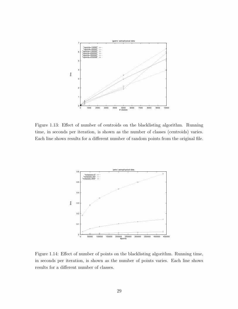
I have conducted experiments with approximate clustering using simulated data.

Again, the results shown are averages over 30 random datasets. Figure 1.16 shows

the effect approximate clustering has on the run-time of the algorithm. We notice

it runs faster than the blacklisting algorithm, with larger speedups as the number of

points increases. It is about 25% faster for 10,000 points, and twice as fast 50, 000

points or more. As for the quality of the output, Figure 1.17 shows the distortion of

the clustering of both algorithms. The distortion of the approximate method is at

most 1% more than the blacklisting clustering distortion (which is exact).

30

0.02

0.04

0.06

0.08

0.1

0.12

0.14

0.16

0.18

0.2

0 20000 40000 60000 80000 100000 120000

time

points

40 classes, 2 dimensions

"BL-approximate""blacklisting"

Figure 1.16: Runtime of approximate clustering Running time, in seconds per it-

eration, is shown as the number of points varies. Each line stands for a different

algorithm.

0.00368

0.00369

0.0037

0.00371

0.00372

0.00373

0.00374

0.00375

0.00376

0.00377

0 20000 40000 60000 80000 100000 120000

dist

ortio

n

points

40 classes, 2 dimensions

"BL-approximate""blacklisting"

Figure 1.17: Distortion for approximate and exact clustering. Each line stands for a

different algorithm.

31

1.6 Related Work

The K-means algorithm is known to converge to a local minimum of the distortion

measure. It is also known to be too slow for practical databases.1 Much of the

related work does not attempt to confront the algorithmic issues directly. Instead,

different methods of subsampling and approximation are proposed. A way to obtain a

small “balanced” sample of points by sampling from the leaves of a R∗ tree is shown

in Ester et al. (1995). In Ng and Han (1994), a simulated-annealing approach is

suggested to direct the search in the space of possible partitions of the input points.

It is also possible to tackle the problem in the deterministic annealing framework

(Hofmann & Buhmann, 1997; Ueda & Nakano, 1998). This is generally believed to

be a robust method. However the author is not aware of any work to improve its

run-time performance or to provide a detailed comparison with standard K-means.

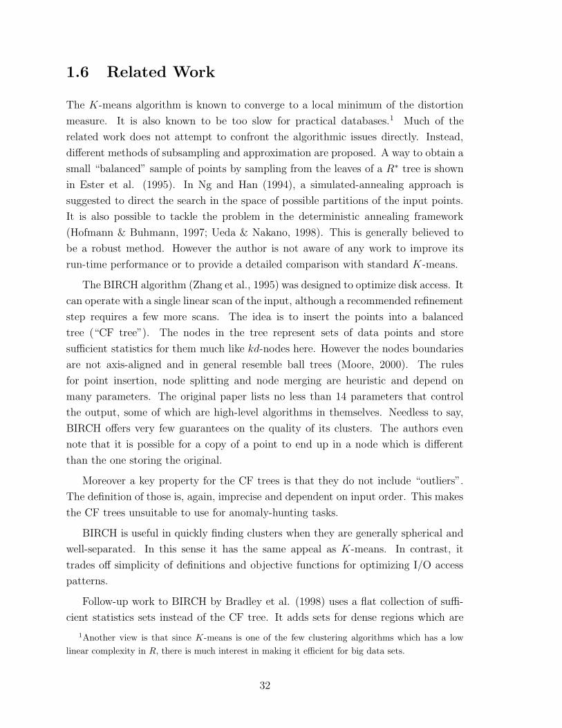
The BIRCH algorithm (Zhang et al., 1995) was designed to optimize disk access. It

can operate with a single linear scan of the input, although a recommended refinement

step requires a few more scans. The idea is to insert the points into a balanced

tree (“CF tree”). The nodes in the tree represent sets of data points and store

sufficient statistics for them much like kd-nodes here. However the nodes boundaries

are not axis-aligned and in general resemble ball trees (Moore, 2000). The rules

for point insertion, node splitting and node merging are heuristic and depend on

many parameters. The original paper lists no less than 14 parameters that control

the output, some of which are high-level algorithms in themselves. Needless to say,

BIRCH offers very few guarantees on the quality of its clusters. The authors even

note that it is possible for a copy of a point to end up in a node which is different

than the one storing the original.

Moreover a key property for the CF trees is that they do not include “outliers”.

The definition of those is, again, imprecise and dependent on input order. This makes

the CF trees unsuitable to use for anomaly-hunting tasks.

BIRCH is useful in quickly finding clusters when they are generally spherical and

well-separated. In this sense it has the same appeal as K-means. In contrast, it

trades off simplicity of definitions and objective functions for optimizing I/O access

patterns.

Follow-up work to BIRCH by Bradley et al. (1998) uses a flat collection of suffi-

cient statistics sets instead of the CF tree. It adds sets for dense regions which are

1Another view is that since K-means is one of the few clustering algorithms which has a low

linear complexity in R, there is much interest in making it efficient for big data sets.

32

not always tied to the same centroid, but when they change their owner they do so

together. Another noteworthy idea is the use of a “worst-case” criterion to estimate

if a point is likely to never change its owner. Unfortunately many details are missing,

and again the user is expected to specify many parameters. This work only evaluates

the quality of the proposed method against a version of K-means which works on a

random sample of the data. No run time analysis is given.

Further improvements are made by Farnstrom et al. (2000). They analyze the

work of Bradley et al. (1998) and note that many of the improvements in fact hurt

the run time. They simplify the data structure and eliminate many user-supplied

parameters. By doing this they were able to reduce the run time from several times

slower than standard K-means, to about twice as fast on some datasets. Since an

inner loop of this algorithm runs K-means on an in-core sample of the data, it can

still take advantage of the work presented here.

A different approach to K-means is suggested by Domingos and Hulten (2001a).

They develop a “Probably Approximately Correct” version of K-means that can

determine when it has seen enough data points to be confident that the output clusters

do not differ by much from ones obtained from infinite data. This is reminiscent of

the algorithm I present for dependency trees in Chapter 4 (and indeed, both were

inspired by the same work). Their results for K-means are promising.

Another approach to exact acceleration is taken by Elkan (2003). He shows how

to use the triangle inequality for both upper and lower bounds on distances between

points and centroids to save distance computations. Large speed-ups for synthetic

and real data with large M and k are reported. The algorithm is still linear in R.

Additionally it requires O(K2) inter-centroid distance computations which in some

cases may be prohibitively high. This work also contains a related work section which

brings together previous publications from many different research communities.

More exact acceleration can be found in Moore (2000). That work builds metric

trees in a unique way and then decorates them with cached sufficient statistics. This

results in a data structure that can use the triangle inequality to prune away big

subsets of points and centroids. Large speedups are demonstrated for blacklisting K-

means, as well as for kernel regression, locally weighted regression, mixture modeling

and Bayes Net learning.

Recall that K-means starts from a set of arbitrary starting locations for the cen-

troids. But once they are given, it is fully deterministic. A bad choice of initial

centroids can have a great impact on both performance and distortion. Bradley and

Fayyad (1998) discuss ways to refine the selection of starting centroids through re-

33

peated sub-sampling and smoothing.

Over the years several modifications to K-means were proposed (Zhang et al.,

2000; Kearns et al., 1997; Hamerly & Elkan, 2002; Bezdek, 1981). They try to address

the “winner takes all” approach of K-means where only one centroid is affected by

each point. The claim is that smoother functions are easier to optimize. For example,

imagine a centroid which is away from its optimal location, but the region between

the current and target location is sparse. Hard assignment will require the centroid

to somehow “leap” over the sparse region, but does not give it a way to “know”

about the distant points. In contrast, soft assignment that gives the centroid low-

weight versions of the distant points might direct the movement correctly. Hamerly

and Elkan (2002) show that the best performer among the surveyed methods is K-

harmonic means (Zhang et al., 2000). It remains an open question if any of these

methods can be accelerated in a similar manner to this work. One hybrid approach,

suggested by Zhang et al. (2000), is to run a few iterations of K-harmonic means to get

over the potentially bad initialization stage, and then feed the output as initialization

points to the faster K-means algorithm, which is known to behave well with good

initialization points. It remains to be seen if distance-based proofs can be used for

algorithms that do not follow the “winner takes all” rule.

Originally, kd-trees were used to accelerate nearest-neighbor queries. We could,

therefore, use them in the K-means inner loop transparently. For this method to work

we will need to store the centroids in the kd-tree. So whatever savings we achieve,

they will be a function of the number of centroids, and not of the (necessarily larger)

number of points. The number of queries will remain R. Moreover, the centroids

move between iterations, and a naive implementation would have to rebuild the kd-

tree whenever this happens. My methods, in contrast, store the entire dataset in the

kd-tree.

The blacklisting idea was published simultaneously and independently by AlSabti

et al. (1999). I stumbled on that paper by chance a while after publication of this

work. Their presentation lacks the geometric proofs, but otherwise seems equivalent.

Elements missing from that work with respect to this one are exhaustive experimen-

tation, and stable-state caching as in Section 1.4.

1.6.1 Improvements over fast mixture-of-Gaussians

At first glance, this work might seem like a specialization of Moore (1998). Both are

similar in that they utilize multiresolution kd-trees. Also, they both implement an

34

EM procedure for a Gaussian mixture model, and they both gain significant speedups.

To counter that, I list the improvements specific to this work. First, the idea of

blacklisting is novel. Moreover, it cannot be easily applied to the soft-membership

model of mixture of general Gaussians. In that framework, each point always affects

all of the centroids. Because the effect of the points furthest away from a centroid is

small, the general Gaussians algorithm may decide to ignore them by pruning branches

of the kd-tree. This introduces approximation into the calculation. In contrast, K-

means is a hard-membership model and blacklisting only eliminates the points which

provably do not belong to a centroid. Therefore my algorithm is exact.

Second, I introduce node caching. It saves a lot of work in regions of the space

which are quiescent. This is a frequent occurrence in late iterations. It appears that

this idea can be retrofitted to the general Gaussians method.

Third, I provide two alternative implementations. One of them only uses geometric

proofs without blacklisting. It is shown in Figure 1.11. It is actually closer in spirit

to the ideas presented in Moore (1998). We can see that it behaves qualitatively

differently than the blacklisting version as the number of dimensions grows. Notice

how there are occasions where it is faster to avoid blacklisting. The exact cross-over

point shown is around seven dimensions, but in practice will depend on the properties

of the data.

1.7 Conclusion

The main message of this chapter is that the well-known K-means algorithm need not

necessarily be considered an impractically slow algorithm, even with many records

and centroids. I have described, analyzed and given empirical results for a new

fast implementation of K-means. I have shown how a kd-tree of all the data points,

decorated with extra statistics, can be traversed with a new, extremely cheap, pruning

test at each node. Another new technique—blacklisting—gives a many-fold additional

speed-up, both in theory and empirically.

For datasets too large to fit in main memory, the same traversal and black-listing

approaches could be applied to an on-disk structure such as an R-tree, permitting

exact K-means to be tractable even for many billions of records.

This method performs badly in high dimensions. This is a fundamental short-

coming of the kd-tree: in each subsequent level it merely splits the data according

to one dimension. But this does not imply the work presented here is only useful on

35

toy problems, for several reasons. First, there are multiple domains where only a few

dimensions are needed. Of these come to mind astrophysics, geo-spatial-data, and

controls. Second, it is possible to first project the data onto a low-dimensional space,

and cluster the projected data.2 In fact there is evidence that such a preprocessing

step might make the clusters more spherical and hence easier to work with. More-

over, even a simple approach such as random projection is sufficient to obtain very

good results — in some cases evading problems which trip a more complex method

such as PCA (Dasgupta, 2000). Third, much of the principles here carry over to

data structures better suited for high dimensional data, such as metric trees (Moore,

2000).

Unlike previous approaches (such as the mrkd-trees for EM in Moore (1998)) this

new algorithm scales very well with the number of centroids, permitting clustering

with tens of thousands of centroids. The need for this kind of performance arises in

cosmology data where a very large number of astronomical objects are examined or

simulated. The structure of large-scale regions of space is summarized in a succinct

representation such as the halo occupation distribution (HOD). Assigning cluster

membership for each galaxy is a precondition to computing the necessary statistic.

My implementation for K-means (shared with the K-means code described in the

following Chapter) is available for researchers3 and was downloaded by over 200 users

as of March 2004. Among others, it was used in the following applications:

• cDNA microarray data. K-means is run repeatedly on a small subset of the

total data (Bainbridge, 2004).

• DNA microarray gene expression levels (Ballini, 2003; Qian, 2001).

• Music information retrieval (Zissimopoulos, 2003).

• Financial data analysis (Kallur, 2003).

• Prediction of functional RNA genes in genomic sequences. The data is clustered

for the purpose of drawing negative examples for the training set. There are

about 700 clusters and more than a million data points (Meraz, 2002).

• Multi-objective optimization with evolutionary algorithms (Koch, 2002).

• Molecular biology (Zhang, 2000).

2There are several ways to transfer the resulting clustering back to the original domain. For

example one can use the class labels to seed a single iteration of an EM fit in the original space.3See http://www.pelleg.org/kmeans.

36

K-means is a well-established algorithm that has prospered for many years as a

clustering algorithm workhorse. Additionally, it is often used to help find starting

clusters for more sophisticated iterative methods such as mixture models. The tech-

niques in this chapter can make such preprocessing steps efficient. Finally, with fast

K-means, we can afford to run the algorithm many times in the time it would usually

take to run it once. This allows automatic selection of k, or subsets of attributes upon

which to cluster, to become a tractable, real-time operation. The following chapter

develops this idea further.

37

Chapter 2

X-means

K-means is well-established as a general clustering solution. It is popularly recom-

mended as the first thing to try, given a new data set. In the last chapter I showed

how to make it scale so it can run on huge data. But in many contexts, it cannot be

immediately used because it requires the user to specify the number of clusters K.

Users who are well acquainted with the data have no problem knowing what K is:

this is typical of clustering in some well researched area where plenty of prior knowl-

edge exists (a biologist, for example, frequently knows how many different species are

represented in the data and can safely assume this will reflect in the clustering). But

this is not always the case. For example, a computer architect may profile a run-

ning program by monitoring its execution. The instructions are grouped, and similar

groups are bundled together to form units of similar execution patterns, or program

phases. It is impossible to know in advance what — and how many — phases an

arbitrary program will go through when run on an arbitrary input. This calls for a

framework to support automatic estimation of K.

Statistical measures to score different models abound. They usually include two

terms. One increases as the fit is improved and the data modeled more accurately.

It is necessary to have this. However, it can be trivially optimized by tweaking the

model and making it more and more complex. Therefore a second penalty term,

which favors simpler models, is normally added.

We leave aside the statistical debate on which scoring function is “best”. Our focus

is how to efficiently compute the score once such a function is chosen. In particular

we want to apply it to K-means clusters. We want it to scale as well as K-means

itself. Additionally, we want an practical way to search over many models. Without

it, we would need to exhaustively search a very large space (for K-means this entails

39

blindly trying many different values for K).

Building on the last chapter, I introduce a new algorithm that efficiently searches

the space of cluster locations and number of clusters to optimize a clustering quality

measure. The innovations include two new ways of exploiting cached sufficient statis-

tics and a new very efficient test that in one K-means sweep selects the most promising

subset of classes for refinement. This gives rise to a fast, statistically founded algo-

rithm that outputs both the number of classes and their parameters. Experiments

show this technique reveals the true number of classes in the underlying distribution,

and that it is much faster than repeatedly using accelerated K-means for different

values of K.

2.1 Introduction

K-means (Duda & Hart, 1973; Bishop, 1995) has long been the workhorse for metric

data. Its attractiveness lies in its simplicity, and in its local-minimum convergence

properties. It has, however, three main shortcomings. One, it is slow and scales

poorly with respect to the time it takes to complete each iteration. Two, the number

of clusters K has to be supplied by the user. Three, when confined to run with a fixed

value of K it empirically finds worse local optima than when it can dynamically alter

K. This chapter offers solutions for these problems. Speed is greatly improved by

embedding the dataset in a multi-resolution kd-tree as described in Chapter 1. This

fast algorithm is used as a building-block in what I call “X-means”: a new algorithm

that quickly estimates K. It goes into action after each run of K-means, making

local decisions about which subset of the current centroids should split themselves in

order to better fit the data. The splitting decision is done by computing the Bayesian

Information Criterion (BIC). I show how the blacklisting method naturally extends

to ensure that obtaining the BIC values for all current centers and their tentative off-

spring costs no more than a single K-means iteration. I further enhance computation

by caching stable-state information and eliminating the need to re-compute it.

I have experimented with X-means against a more traditional method that esti-

mates the number of clusters by guessing K. X-means consistently produced better

clustering on both synthetic and real data, with respect to BIC. It also runs much

faster, even when the baseline is my accelerated blacklisting K-means.

The rest of the chapter is organized as follows. In Section 2.2 I discuss prior work

and introduce notation. My algorithms are presented in Section 2.3, which briefly

discusses blacklisting and outlines fast BIC computation. It also expands on BIC

40

and touches on alternative goodness-of-fit measures. I show experimental results in

Section 2.4, and conclude in Section 2.5.

2.2 Definitions

I first briefly describe the naive K-means algorithm for producing a clustering of the

points in the input into K clusters. It partitions the data points into K subsets such

that all points in a given subset “belong” to some center. The algorithm keeps track

of the centroids of the subsets, and proceeds in iterations. Before the first iteration

the centroids are initialized to arbitrary values. The algorithm terminates when the

centroid locations stay fixed during an iteration. For a more detailed description and

a literature survey refer to Chapter 1.

For the remainder of this paper we denote by µj the coordinates of the j-th

centroid. We will use the notation (i) to denote the index of the centroid which is

closest to the i-th data point. For example, µ(i) is the centroid associated by the i-th

point during an iteration. D is the input set of points, and Di ⊆ D is the set of points

that have µi as their closest centroid. We let R = |D| and Ri = |Di|. The number of

dimensions is M , and the Gaussian covariance matrix is Σ = diag(σ2).

2.3 Estimation of K

The algorithm as it was described up to this point can only be used to perform K-

means where K is fixed and supplied by the user. This is a reasonable requirement if K

is small or if a strong prior exists. For example, a biologist might collect measurements

on seven different species of an organism, and then run K-means with K set to 7. But

in many other applications, we do not have this privilege. For example, a computer

program execution can be traced and the instructions grouped into blocks (Sherwood

et al., 2002). Now we would like to group the blocks and define different phases of

the program execution. The number of phases for an arbitrary program it unknown

in advance, and needs to be estimated as well.

We proceed now to demonstrate how to efficiently search for the best K. The

framework now changes so the user only specifies a range in which the true K reason-

ably lies1, and the output is not only the set of centroids, but also a value for K in

this range which scores best by some model selection criterion. Note that using the

1We allow the range to be [2..R], but in practice much better bounds can be given.

41

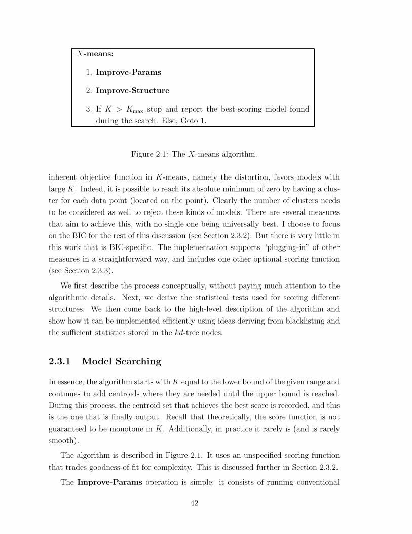
X-means:

1. Improve-Params

2. Improve-Structure

3. If K > Kmax stop and report the best-scoring model found

during the search. Else, Goto 1.

Figure 2.1: The X-means algorithm.

inherent objective function in K-means, namely the distortion, favors models with

large K. Indeed, it is possible to reach its absolute minimum of zero by having a clus-

ter for each data point (located on the point). Clearly the number of clusters needs

to be considered as well to reject these kinds of models. There are several measures

that aim to achieve this, with no single one being universally best. I choose to focus

on the BIC for the rest of this discussion (see Section 2.3.2). But there is very little in

this work that is BIC-specific. The implementation supports “plugging-in” of other

measures in a straightforward way, and includes one other optional scoring function

(see Section 2.3.3).

We first describe the process conceptually, without paying much attention to the

algorithmic details. Next, we derive the statistical tests used for scoring different

structures. We then come back to the high-level description of the algorithm and

show how it can be implemented efficiently using ideas deriving from blacklisting and

the sufficient statistics stored in the kd-tree nodes.

2.3.1 Model Searching

In essence, the algorithm starts with K equal to the lower bound of the given range and

continues to add centroids where they are needed until the upper bound is reached.

During this process, the centroid set that achieves the best score is recorded, and this

is the one that is finally output. Recall that theoretically, the score function is not

guaranteed to be monotone in K. Additionally, in practice it rarely is (and is rarely

smooth).

The algorithm is described in Figure 2.1. It uses an unspecified scoring function

that trades goodness-of-fit for complexity. This is discussed further in Section 2.3.2.

The Improve-Params operation is simple: it consists of running conventional

42

K-means to convergence.

The Improve-Structure operation finds out if and where new centroids should

appear. This is achieved by letting some centroids split in two. How can we decide

what to split? We begin by describing and dismissing two obvious strategies, after

which I will combine their strengths and avoid their weaknesses in my X-means

strategy.

Splitting idea 1: One at a time. The first idea would be to pick one centroid,

produce a new centroid nearby, run K-means to completion and see if the re-

sulting model scores better. If it does, accept the new centroid. If it doesn’t,

return to the previous structure. But this will need O(Kmax) Improve-Params

steps until X-means is complete. This begs the question of how to choose which

centroid is most deserving to give birth. Having answered that we face another

issue: if it doesn’t improve the score what should be tried next? Perhaps all

centroids could be tested in this way (and then we stick with the best) but

since each test needs a run of K-means that would be an extremely expensive

operation for adding only one centroid.

Splitting idea 2: Try half the centroids. Simply choose (say) half the centroids

according to some heuristic criterion for how promising they are to split. Split

them, run K-means, and see if the resulting model scores better than the orig-

inal. If so accept the split. This is a much more aggressive structure im-

provement, requiring only O(log Kmax) Improve-Params steps until X-means

completes. But what should the heuristic criterion be? Size of region owned by

centroid? Distortion due to centroid? Furthermore, we will miss the chance to

improve in cases when one or two centroids need to split but the rest do not.

My solution achieves the benefits of ideas 1 and 2, but avoids the drawbacks and can

be turned into an extremely fast operation (as we will see in Section 2.3.4). I will

explain by means of an example.

Figure 2.2 shows a stable K-means solution with 3 centroids. The boundaries

of the regions owned by each centroid are also shown. The structure improvement

operation begins by splitting each centroid into two children (Figure 2.3). They are

moved a distance proportional to the size of the region in opposite directions along a

randomly chosen vector. Next, in each parent region we run a local K-means (with

K = 2) for each pair of children. It is local in that the children are fighting each other

for the points in the parent’s region: no others. Figure 2.4 shows the first step of all

43

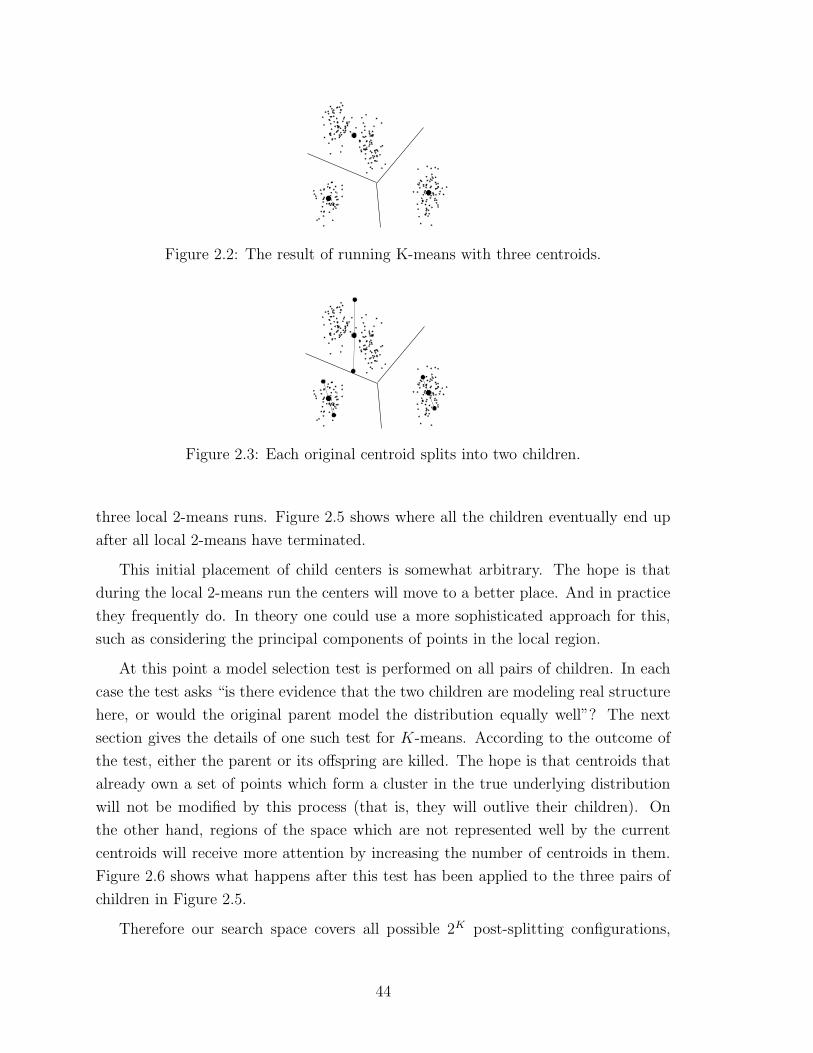
Figure 2.2: The result of running K-means with three centroids.

Figure 2.3: Each original centroid splits into two children.

three local 2-means runs. Figure 2.5 shows where all the children eventually end up

after all local 2-means have terminated.

This initial placement of child centers is somewhat arbitrary. The hope is that

during the local 2-means run the centers will move to a better place. And in practice

they frequently do. In theory one could use a more sophisticated approach for this,

such as considering the principal components of points in the local region.

At this point a model selection test is performed on all pairs of children. In each

case the test asks “is there evidence that the two children are modeling real structure

here, or would the original parent model the distribution equally well”? The next

section gives the details of one such test for K-means. According to the outcome of

the test, either the parent or its offspring are killed. The hope is that centroids that

already own a set of points which form a cluster in the true underlying distribution

will not be modified by this process (that is, they will outlive their children). On

the other hand, regions of the space which are not represented well by the current

centroids will receive more attention by increasing the number of centroids in them.

Figure 2.6 shows what happens after this test has been applied to the three pairs of

children in Figure 2.5.

Therefore our search space covers all possible 2K post-splitting configurations,

44

Figure 2.4: The first step of parallel local 2-means. The line coming out of each

centroid shows where it moves to.

BIC(k=1)=2018BIC(k=2)=1859

BIC(k=2)=1784

BIC(k=1)=2471BIC(k=2)=3088

BIC(k=1)=1935

Figure 2.5: The result after all parallel 2-means have terminated.

BIC(k=1)=2018BIC(k=2)=1859

BIC(k=2)=1784

BIC(k=1)=2471BIC(k=2)=3088

BIC(k=1)=1935

Figure 2.6: The surviving centroids after all the local model scoring tests.

45

and it determines which one to explore by improving the BIC locally in each region.

Compared with ideas 1 and 2 above, this allows an automatic choice of whether to

increase the number of centroids by very few (in case the current number is very close

to the true number) or very many (when the current model severely underestimates

K). Empirically, I have also found that regional K-means runs with just 2 centers

tend to be less sensitive to local minima.

We continue oscillating between Improve-Params and Improve-Structure un-

til the upper bound for K is attained. The implementation uses the following rule to

handle the case of a worsening score with increasing K. If no centroids seem worse

than their children, the difference between BIC score of parent and their respective

children centroids is calculated. The parents are then ranked by this value, and the

top 50% are forcibly split.

It remains to discuss the cost of running K-means together with BIC evaluation.

We return to this issue after a short digression to statistical scoring.

2.3.2 BIC Scoring

Assume we are given the data D and a family of alternative models Mj, where in our

case different models correspond to solutions with different values of K. How do we

choose the best? Intuitively we would like to balance goodness of fit (which can be

improved by enriching the model with more parameters) and model simplicity (which

implies few parameters).

More precisely, we will use the posterior probabilities Pr[Mj|D] to score the mod-

els. In our case the models are all of the type assumed by K-means (that is, spherical

Gaussians). To approximate the posteriors, up to normalization, we use the following

formula from Kass and Wasserman (1995):

BIC(Mj) = lj(D)− pj

2· log R

where lj(D) is the log-likelihood of the data according to the j-th model and taken

at the maximum-likelihood point, and pj is the number of parameters in Mj. This is

also known as the Schwarz criterion (Wasserman, 1997).

The maximum likelihood estimate (MLE) for the variance, under the identical

spherical Gaussian assumption, is:

σ2 =1

R−K

∑

i

(xi − µ(i))2 .

46

The point probabilities are:

P (xi) =R(i)

R· 1√

2π||Σ||1/2exp

(

− 1

2σ2||xi − µ(i)||2

)

=R(i)

R· 1√

2πσMexp

(

− 1

2σ2||xi − µ(i)||2

)

.

The log-likelihood of the data is:

l(D) = log∏

i P (xi) =∑

i

(

log 1√2πσM

− 12σ2 ||xi − µ(i)||2 + log

R(i)

R

)

.

Fix 1 ≤ n ≤ K. Focusing just on the set Dn of points which belong to centroid n

and plugging in the maximum likelihood estimates yields:

l(Dn) = −Rn

2log(2π)− Rn ·M

2log(σ2)− Rn −K

2+Rn log Rn − Rn log R .

The number of free parameters pj is simply the sum:

• K − 1 class probabilities (the last one is redundant since they sum to one).

• M ·K centroid coordinates.

• One variance estimate.

To extend this formula for all centroids instead of one, we use the fact that the

log-likelihood of the points that belong to all centroids in question is the sum of the

log-likelihoods of the individual centroids, and replace R above with the total number

of points which belong to the centroids under consideration.

We use the BIC formula in two places: globally when X-means finally chooses the

best model it encountered, and also locally in all the centroid split tests.

2.3.3 Anderson-Darling Scoring

Recently, Hamerly and Elkan analyzed the BIC criteria as used in X-means and

found cases where it can over-estimate k. For the full treatment see Hamerly and

Elkan (2003). I provide a short summary here for completeness.

47

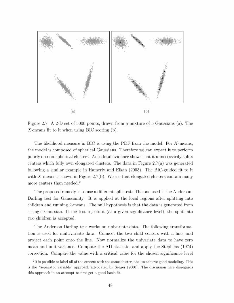
(a) (b)

Figure 2.7: A 2-D set of 5000 points, drawn from a mixture of 5 Gaussians (a). The

X-means fit to it when using BIC scoring (b).

The likelihood measure in BIC is using the PDF from the model. For K-means,

the model is composed of spherical Gaussians. Therefore we can expect it to perform

poorly on non-spherical clusters. Anecdotal evidence shows that it unnecessarily splits

centers which fully own elongated clusters. The data in Figure 2.7(a) was generated

following a similar example in Hamerly and Elkan (2003). The BIC-guided fit to it

with X-means is shown in Figure 2.7(b). We see that elongated clusters contain many

more centers than needed.2

The proposed remedy is to use a different split test. The one used is the Anderson-

Darling test for Gaussianity. It is applied at the local regions after splitting into

children and running 2-means. The null hypothesis is that the data is generated from

a single Gaussian. If the test rejects it (at a given significance level), the split into

two children is accepted.

The Anderson-Darling test works on univariate data. The following transforma-

tion is used for multivariate data. Connect the two child centers with a line, and

project each point onto the line. Now normalize the univariate data to have zero

mean and unit variance. Compute the AD statistic, and apply the Stephens (1974)

correction. Compare the value with a critical value for the chosen significance level

2It is possible to label all of the centers with the same cluster label to achieve good modeling. This

is the “separator variable” approach advocated by Seeger (2000). The discussion here disregards

this approach in an attempt to first get a good basic fit.

48

and accept or reject the null hypothesis. Tables for critical values can be found in

Hamerly (2003).

Since published, the AD test has been incorporated into the X-means implemen-

tation. The user can choose to use it in the local decision step instead of the BIC

test. The global test used is still BIC. Optionally, the run can be terminated as soon

as no centers are split (instead of forcibly splitting some centers so as to reach Kmax).

2.3.4 Acceleration

The X-means algorithm described so far can be implemented as-is for small datasets.

But so far we neglected its most important feature. It was invented subject to the

design constraint that it should be possible to use cached statistics to scale it up

to datasets with massive numbers of records. Much of the material here appears in

more detail in Chapter 1. Those familiar with that material can safely skip ahead.

Others will probably need the context given here to appreciate the X-means specific

additions described later.

Accelerating K-means

We begin by concentrating on a single K-means iteration. The task is to determine,

for every data point, which centroid owns it. Then, we can compute the center-of-mass

of all points which belong to a given centroid and that defines the new location for that

centroid. Immediately we observe that showing that a subset of points all belong to a

given centroid is just as informative as doing this for a single point, given that we have

sufficient statistics for the subset (in our case the sufficient statistics are the number

of points and their vector sum). Clearly it may save a lot of computation, provided

that doing this is not significantly more expensive than demonstrating the ownership

over a single point. Since the kd-tree imposes a hierarchical structure on the data

set, and we can easily compute sufficient statistics for its nodes at construction time,

it makes a natural selection for the partition of the points. Each kd-node represents

a subset of the data set. It also has a bounding box, which is a minimal axis-parallel

hyper-rectangle that includes all points in the subset. In addition it contains pointers

to two children nodes, which represent a bisection of the points their parent owns.

Consider a set of counters, one for each centroid, which store a running total of the

number of points that belong to each, as well as their vector sum. We now show how

to update all the counters by scanning the kd-tree just once. The Update procedure

49

is a recursive one, and accepts as parameters a node and a list of centroids that may

own the points in it. Its task is to update the counters of the nodes in question with

the appropriate values of the points in the node. The initial invocation is with the root

node and the list of all centroids. After it returns, the new locations may be calculated

from the counters. The procedure considers the geometry of the bounding box and

the current centroid locations to eliminate centroids from the list by proving they

cannot possibly own any point in the current node. Hence the name “blacklisting”.

The point to remember here is that after shrinking the list, the procedure recurses on

the children of the current node. The halting condition is met when the list contains

just one centroid; then, the centroid’s counters are incremented using the statistics

stored in the kd-node. Frequently this happens in a shallow level of the kd-tree, and

eliminates the work needed to traverse all of its descendants.

Accelerating Improve-Structure

The procedure described above works well to update the centroid locations of a global

K-means iteration. We will now apply the same procedure to carry forward an

Improve-Structure step. Recall that during Improve-Structure we perform 2-

means in each Voronoi region of the current structure. We carry this out by first

making a list of the parent centroids, and use that as input to the Update procedure.

The difference from the global iteration is in the action taken when the list reduces to a

single centroid. This event signifies the fact that all points in the current node belong

to the single centroid (equivalently, that it is fully contained in a Voronoi region). We

now know for certain that the points in the node can only affect a local 2-means step.

To quantify this effect we divide the points between the children according to their

location. Recall that this is exactly what Update does, when given the appropriate

node and centroid list. Specifically, we create a new centroid list containing just the

two children, and recurse on Update using this short list and the current node. The

rest of the work is done by the Update procedure. After a full scan of the kd-tree

has been carried out (possibly pruning away many nodes), the counters of the child

centroids have their final values and their new locations can be computed. Now a

new iteration can take place, and so on until the last of the centroid pairs has settled

down. To emphasize, in a single traversal of the kd-tree we handle all of the parents

and all of their children.

50

Additional Acceleration

An interesting outcome of the local decision-making is that some regions of the space

tend to become active (i.e., a lot of splitting and re-arrangement takes place) while

other regions, where the centroids seem to have found the true classes, appear dor-

mant. We can translate this pattern into further acceleration by using caching of

statistics from previous iterations. Consider a kd-node that contains a boundary be-

tween two centroids (that is, either of the two centroids may own any of the node’s

points). Although we must recurse down the tree in order to update the counters for

the centers, there is no reason to do this again in the next iteration, provided that the

centroids did not move, and that no other centroid has moved into a position such

that it can own any of the node’s points. We therefore cache the contribution of this

node to each of the centroids’ counters in the node, and subsequent iterations do not

need to traverse the tree any further than the current node if the list of competing

centroids matches.

To enable fast comparison of centroid locations against their position in previous

iterations we once again employ a write-once data structure which does not permit

alteration of centroid coordinates after the initial insertion. In case a centroid location

changes, a new element has to be inserted and it is given a unique identifier. This

way only a O(1) comparison of identifiers (per centroid) is needed. Clearly “old”

centroids would never be accessed so there is no need to keep storing them in the

data-structure. This allows for a fast and memory-efficient implementation using the

original M ·K memory plus a hash-table for identifier lookup.

A further extension of this idea can also cache the children of a centroid in a

regional iteration. Consider the following scenario. Some centroid is rejecting a split

into children. Suppose it does not move, and at the next iteration we try to split it

again. We want to reuse the information on children nodes (which have no reason

to change this time) and save computation. To achieve this, we do not kill children

node and instead move them to a “zombie” state. The next regional iteration will

resurrect them. Owing to the fact that their identifiers did not change, the caching

mechanism immediately recalls the outcome of their last local iteration (which may

have been reached after several re-positioning steps). We finally remove children from

the data structure when their parent is killed (in our write-once data scheme, this

happens when the parent moves).

51

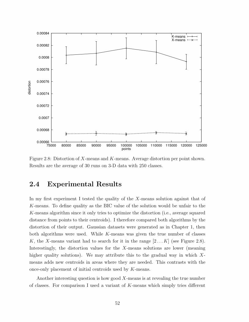
0.00066

0.00068

0.0007

0.00072

0.00074

0.00076

0.00078

0.0008

0.00082

0.00084

75000 80000 85000 90000 95000 100000 105000 110000 115000 120000 125000

dist

ortio

n

points

K-meansX-means

Figure 2.8: Distortion of X-means and K-means. Average distortion per point shown.

Results are the average of 30 runs on 3-D data with 250 classes.


In my first experiment I tested the quality of the X-means solution against that of

K-means. To define quality as the BIC value of the solution would be unfair to the

K-means algorithm since it only tries to optimize the distortion (i.e., average squared

distance from points to their centroids). I therefore compared both algorithms by the

distortion of their output. Gaussian datasets were generated as in Chapter 1, then

both algorithms were used. While K-means was given the true number of classes

K, the X-means variant had to search for it in the range [2 . . .K] (see Figure 2.8).

Interestingly, the distortion values for the X-means solutions are lower (meaning

higher quality solutions). We may attribute this to the gradual way in which X-

means adds new centroids in areas where they are needed. This contrasts with the

once-only placement of initial centroids used by K-means.

Another interesting question is how good X-means is at revealing the true number

of classes. For comparison I used a variant of K-means which simply tries different

52

Table 2.1: The mean absolute error vs. the number of classes output by the two

algorithms, using 2-D data with 4000 to 36000 points.

classes error

K-means X-means

50 3.53± 0.37 3.00± 0.89

100 5.77± 0.58 9.06± 1.00

150 9.65± 4.28 21.43± 2.26

values of K and reports the configuration which resulted in the best BIC. This differs

from X-means in that for each K a new search is started. In contrast, X-means

add new centers in very particular locations, based on the outcome of the preceding

K-means run.

The permissible range for X-means was [2 . . . 2K], and for K-means I used the

20 equally-distant values up to 2K. Averaged results are in Table 2.1 and detailed

results for the 100-class case are in Figure 2.9. They show that X-means outputs

a configuration which is within 15% from the true number of classes. We also see

that K-means does better in this respect (about 6% average deviation). The results

also show that K-means tends to over-estimate the number of classes, and also to

output more classes as the number of records, R, increases, while X-means usually

under-estimates the true K, and is in general insensitive to R.

I also show an updated version of Table 1.2 in Table 2.2. It again shows that X-

means under-estimates K. Note that in this experiment K-means was now allowed

to search over K.

A slightly different picture arises when we examine the BIC score of the output

configurations. Note that my K-means variant chooses the best configuration by its

BIC score, so this is a fair comparison now. In Figure 2.10 we see that X-means scores

not only better than K-means in this respect, but also outperforms the underlying

distribution which was used to generate the data. This may be explained by random

deviations in the data that cause it to be better modeled by fewer classes than there

actually are. For example, two (or more) class centers, which are chosen at random,

may fall extremely close to one another so they approximate a single class.

As far as speed is concerned, X-means scales much better than iterated K-means.

As shown in Figure 2.11, X-means runs twice as fast for large problems. Note this

53

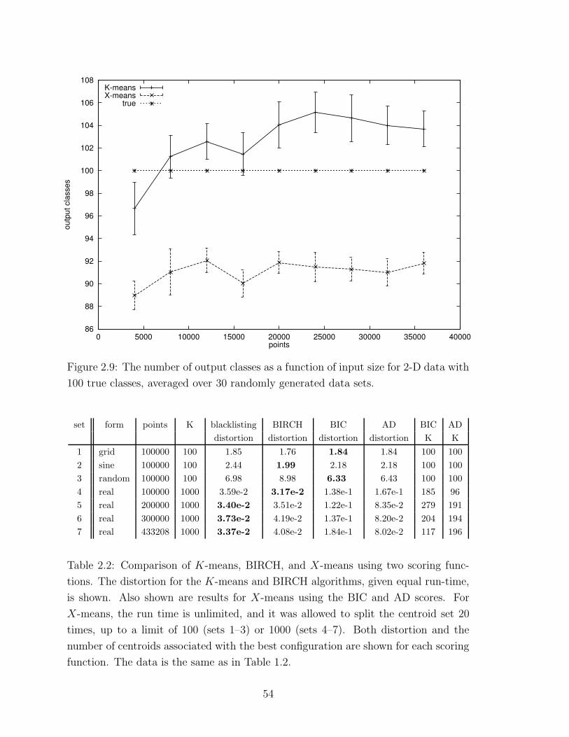
86

88

90

92

94

96

98

100

102

104

106

108

0 5000 10000 15000 20000 25000 30000 35000 40000

outp

ut c

lass

es

points

K-meansX-means

true

Figure 2.9: The number of output classes as a function of input size for 2-D data with

100 true classes, averaged over 30 randomly generated data sets.

set form points K blacklisting BIRCH BIC AD BIC AD

distortion distortion distortion distortion K K

1 grid 100000 100 1.85 1.76 1.84 1.84 100 100

2 sine 100000 100 2.44 1.99 2.18 2.18 100 100

3 random 100000 100 6.98 8.98 6.33 6.43 100 100

4 real 100000 1000 3.59e-2 3.17e-2 1.38e-1 1.67e-1 185 96

5 real 200000 1000 3.40e-2 3.51e-2 1.22e-1 8.35e-2 279 191

6 real 300000 1000 3.73e-2 4.19e-2 1.37e-1 8.20e-2 204 194

7 real 433208 1000 3.37e-2 4.08e-2 1.84e-1 8.02e-2 117 196

Table 2.2: Comparison of K-means, BIRCH, and X-means using two scoring func-

tions. The distortion for the K-means and BIRCH algorithms, given equal run-time,

is shown. Also shown are results for X-means using the BIC and AD scores. For

X-means, the run time is unlimited, and it was allowed to split the centroid set 20

times, up to a limit of 100 (sets 1–3) or 1000 (sets 4–7). Both distortion and the

number of centroids associated with the best configuration are shown for each scoring

function. The data is the same as in Table 1.2.

54

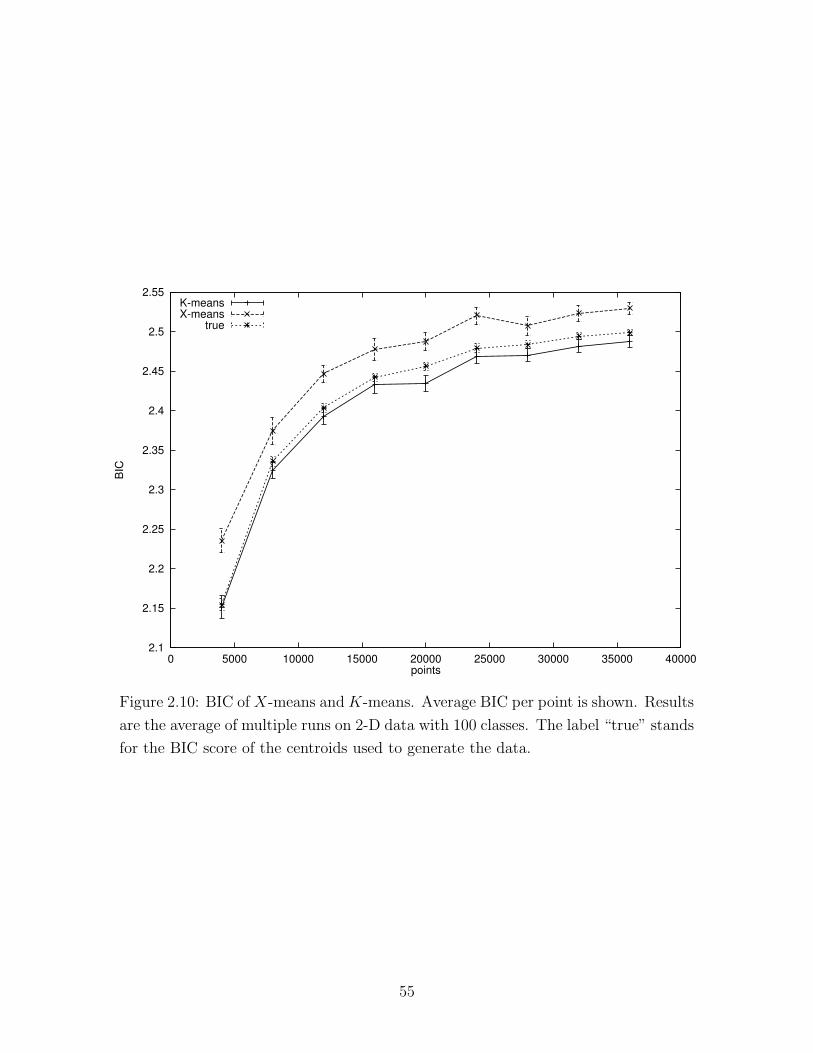
2.1

2.15

2.2

2.25

2.3

2.35

2.4

2.45

2.5

2.55

0 5000 10000 15000 20000 25000 30000 35000 40000

BIC

points

K-meansX-means

true

Figure 2.10: BIC of X-means and K-means. Average BIC per point is shown. Results

are the average of multiple runs on 2-D data with 100 classes. The label “true” stands

for the BIC score of the centroids used to generate the data.

55

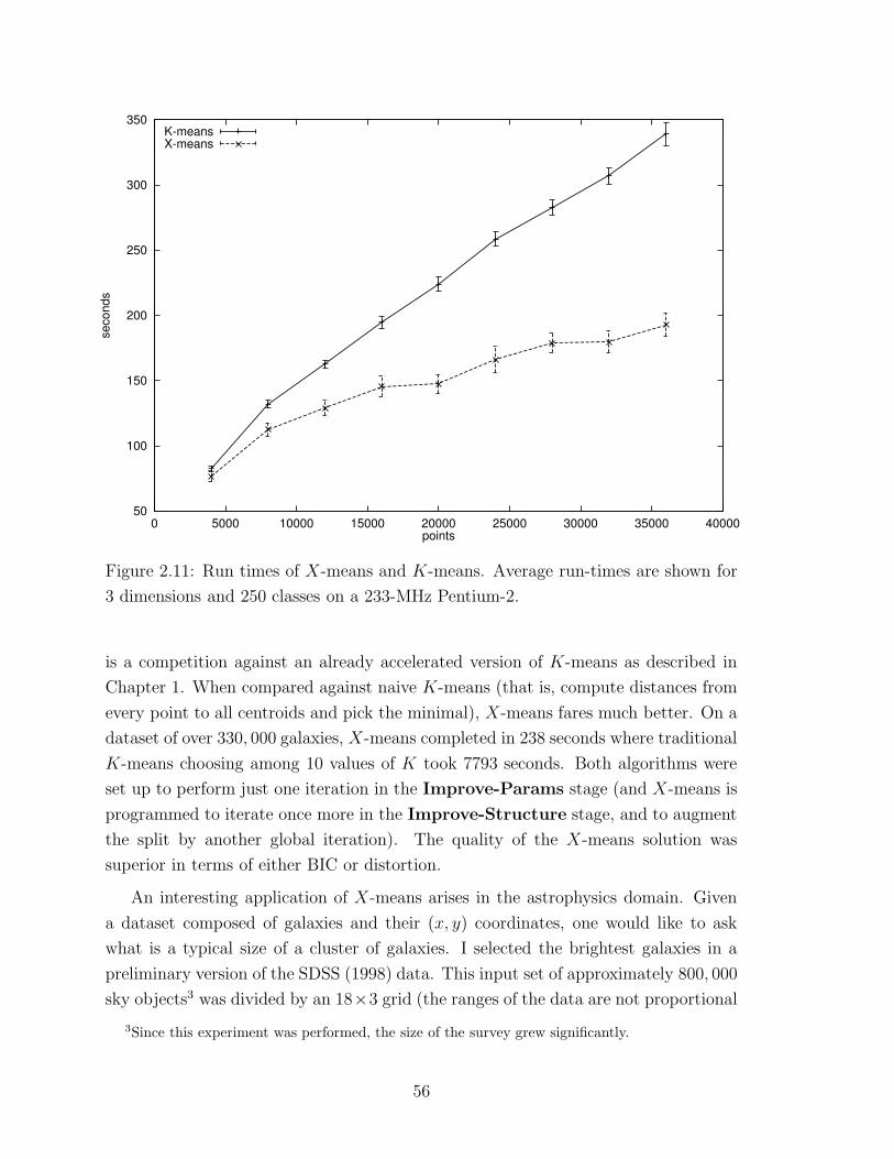
50

100

150

200

250

300

350

0 5000 10000 15000 20000 25000 30000 35000 40000

seco

nds

points

K-meansX-means

Figure 2.11: Run times of X-means and K-means. Average run-times are shown for

3 dimensions and 250 classes on a 233-MHz Pentium-2.

is a competition against an already accelerated version of K-means as described in

Chapter 1. When compared against naive K-means (that is, compute distances from

every point to all centroids and pick the minimal), X-means fares much better. On a

dataset of over 330, 000 galaxies, X-means completed in 238 seconds where traditional

K-means choosing among 10 values of K took 7793 seconds. Both algorithms were

set up to perform just one iteration in the Improve-Params stage (and X-means is

programmed to iterate once more in the Improve-Structure stage, and to augment

the split by another global iteration). The quality of the X-means solution was

superior in terms of either BIC or distortion.

An interesting application of X-means arises in the astrophysics domain. Given

a dataset composed of galaxies and their (x, y) coordinates, one would like to ask

what is a typical size of a cluster of galaxies. I selected the brightest galaxies in a

preliminary version of the SDSS (1998) data. This input set of approximately 800, 000

sky objects3 was divided by an 18×3 grid (the ranges of the data are not proportional

3Since this experiment was performed, the size of the survey grew significantly.

56

in both axis). The cells had approximately the same number of objects. On each cell

with R objects I ran K-means iterated over the 10 values in the range [R/1000, R/100]

and X-means searching for K in the same range, and recorded the resulting number

of clusters (equivalently, the average cluster size).

The average cluster size according to X-means was 473 ± 25.5, and 572 ± 40.8

according to K-means. While it is hard to validate these manually, I tend to believe

X-means since it is free to choose the number of clusters from a wide range where

K-means can only validate a small number of specified K. This fact is well reflected

in the smaller variance of the X-means output. In early experiments, where the range

for K was large and the number of sample points small, this effect was more noticeable

(see Figure 2.12).

In terms of run-time, X-means is not only faster, but increases its advantage as

the number of points increases, similarly to the way it does so for synthetic datasets.

An X-means run over the full data set of some 800, 000 points and 4, 000 resulting

centroids takes about 4.5 hours on a 600-MHz DEC Alpha. A similar K-means

invocation ran into a hard-coded limit after running for twice as long.

In a similar experiment on the important task of clustering galaxies in the LCRS

(1998) data I compared X-means against a highly optimized but traditional (i.e, no

kd-tree) implementation of K-means. Traditional K-means tried 10 different values

of K between 50 and 500. Both algorithms found solutions with almost identical BIC

scores, though X-means chose a larger value of K. X-means completed its search

eight times faster than K-means.

2.5 Conclusion

I have presented a new K-means based algorithm that incorporates model selection.

By adopting and extending algorithmic improvements to K-means, it is efficient to

the extent that running it once is cheaper than looping over K with the fixed-model

algorithm. It uses statistically-based criteria to make local decisions that maximize

the model’s posterior probabilities. Experimental results on both synthetic and real-

life data show it is performing faster and better than K-means.

My implementation for X-means and K-means is available for researchers4 and

was downloaded by over 200 users as of March 2004. It was used for the following

applications:

4See http://www.pelleg.org/kmeans.

57

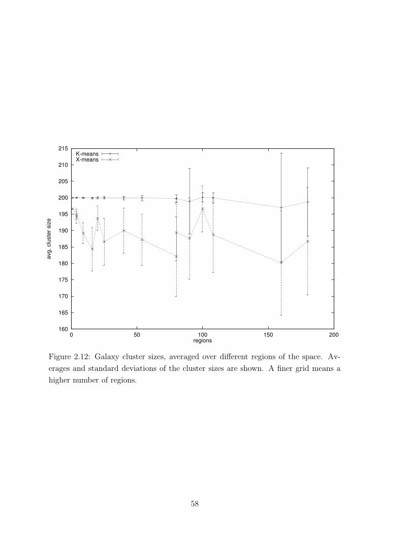
160

165

170

175

180

185

190

195

200

205

210

215

0 50 100 150 200

avg.

clu

ster

siz

e

regions

K-meansX-means

Figure 2.12: Galaxy cluster sizes, averaged over different regions of the space. Av-

erages and standard deviations of the cluster sizes are shown. A finer grid means a

higher number of regions.

58

• Music information retrieval (Logan & Salomon, 2001). Multiple features vectors

are extracted for each one of 8500 songs. A specialized inter-cluster distance

metric is used to determine a distance matrix for song similarity.

• Computer program analysis in the Daikon package (Ernst et al., 2001). Likely

invariants for a program are detected dynamically. To determine conditional

properties of the program, clustering is performed on the invariants.

• Natural language processing (Kruengkrai, 2004).

• Computer architecture (Sherwood et al., 2002). A large trace (several billion

instructions) of a computer program is taken. Instructions are grouped into

basic blocks. Time intervals of a program’s execution are represented by a

vector of counts of the times each basic block was executed. The vectors are

clustered to determine phases in the program’s execution.

• Speaker identification.

• Image segmentation (Kruengkrai, 2004).

In addition, after its publication, the algorithm was independently implemented

in the popular Weka package (Witten & Frank, 2000). The BIC scoring measure was

analyzed and refined by Hamerly and Elkan (2003).

The choice of BIC as the splitting criterion is not the only possible one. While

I have found BIC to perform well for my test-sets and applications, using other

criteria, such as AIC or the Anderson-Darling test may make sense in other areas.

Incorporating such measures into my algorithm is straightforward: AIC is trivial since

all the sub-expressions for it are needed in the BIC formula. The Anderson-Darling

measure was retrofitted following the publication of Hamerly and Elkan (2003) and

required only minor code changes. Therefore, we may classify this work as a whole

new family of algorithms that differ only in their local optimization criteria.

Another direct extension is the application of BIC (or similar criteria) to direct a

model search in an unrestricted-Gaussian EM algorithm (since blacklisting is assuming

hard membership, this is non-trivial). One can also think of other ways to conduct

the search for a model, even under the K-means assumption (e.g., removing centroids,

as well as adding them).

Using my algorithms, statistical analysis of millions of data points and thousands

of classes is performed in a matter of hours. Consequently, we are able to test as-

trophysical theories using observations that are much larger in scale than were ever

59

available in the past. As hinted above, this work opens up an opportunity for a large

class of algorithms to aid in such endeavors.

Finally, we need to consider the question of the dimensionality of the data. This

paper has only empirically demonstrated X-means on up to four-dimensional data,

although simpler algorithms (e.g., fast K-means) still give significant accelerations up

to seven dimensions. But are even seven dimensions enough to be interesting? I say

yes for three reasons.

First, many big-science disciplines need to cluster data sets with between mil-

lions and billions of low-dimensional records very quickly. Spatial galaxy, color-space

sky objects, and protein gel clustering are just three such examples on which I am

collaborating with natural scientists.

Second, for high-dimensional data sets it is frequently preferable to model the

PDF by a factored representation (Meila, 1999b) such as a Bayesian network in which

node distributions can be represented by lower-dimensional clusters. X-means is a

step towards a fast inner-loop for these expensive algorithms.

Finally, it is possible to implement the regional splitting steps efficiently in high

dimensions using ball trees (Moore, 2000), similarly to the way it is done with the

fast version of K-means.

60

Chapter 3

Mixtures of Rectangles

Imagine an end-user of a clustering tool, seeking help with important decisions such as

credit approval. A popular and general tool for clustering is the mixtures-of-Gaussians

model. This is a powerful tool which allows for a wide variety of cluster shapes. It

can be fitted accurately and quickly with the EM method. On the surface it looks

appropriate for clustering the applicants into credit-worthy and others.

So far, our user has no trouble in taking the output of a Gaussian mixture learner

and using it for decision making. But if he or she would also like to know why a

particular applicant is rejected, the only way they have to do that is to examine

the PDF, namely a mixture of Gaussians. In arithmetic terms, this boils down to

subtractions and multiplications of record attributes, most probably represented in

different, often incomparable, units. This kind of obscure manipulation does not

inspire confidence in the outcome of the operation.

What I suggest is choosing a model that is aesthetically pleasing, even if the price

is reduced expressiveness. This way, the cluster definitions themselves can be used di-

rectly in the application domain both for classification and for reasoning. Specifically,

I fit the data to a mixture model in which each component is a hyper-rectangle in

M -dimensional space. Hyper-rectangles may overlap, meaning some points can have

“soft” membership in several components. Each component is simply described by,

for each attribute, lower and upper bounds of points in the cluster.

The computational problem of finding a locally maximum-likelihood collection of

k rectangles is made practical by allowing the rectangles to have soft “tails” in the

early stages of an EM-like optimization scheme. My method requires no user-supplied

parameters except for the desired number of clusters. These advantages make it highly

attractive for “turn-key” data-mining applications. I demonstrate the usefulness of

61

the method in subspace clustering for synthetic data, and in real-life datasets. I also

show its effectiveness in a classification setting.

3.1 Introduction

My model is a mixture of uniform density M -dimensional hyper-rectangles, supple-

mented with Gaussian “tails”. The tails mean that (as is the case with conventional

Gaussians), the probability of a data point decreases with the distance from the “cen-

troid”. But, in contrast to conventional Gaussians, there is a difference in the way we

measure distances. We consider the distance from the point to the closest point to

it that is still included in the rectangular kernel. Note that under this definition all

points contained in the kernel are equally (and maximally) likely. We fit the model

by means of an EM procedure. Finally, we report the rectangular kernels. These

are just lists of intervals (one interval per dimension, per cluster) the intersection of

which defines the dense regions. This model has just O(M) parameters, as opposed

to O(M2) for mixtures of Gaussians. However, it is likely to require more components

than the more general Gaussian-based model.

The difference between soft and hard membership is important to understand.

With hard membership, each element belongs to exactly one class. This is intuitive to

understand and makes sense in the original data domain. I also showed how this very

property enables acceleration of K-means and related algorithms, by eliminating from

the computation the elements which can be proven not to own a point. The problem

with hard membership models is that they are harder to optimize directly. They

have lower resilience to bad initial configuration and may ignore better configurations

that are “nearby” (Zhang et al., 2000; Hamerly & Elkan, 2002). In contrast, soft

membership models have smooth objective functions that are easy to manipulate and

optimize. The downside is the loss of direct interpretation of the model in simple

terms. Often, the consumer of the model now needs to reconcile statements of the

form “this element is 67% in class A and 30% in class B”. What I propose below

offers the simplicity of hard membership with the amenability of soft models.

Much of the related work in the area of clustering is concerned with scaling of the

algorithms to support huge datasets. CLARANS (Ng & Han, 1994) performs a search

over the space of centroids for a k-means model (Duda & Hart, 1973; Bishop, 1995).

BIRCH (Zhang et al., 1995) aims to scale this to massive datasets by concentrating

on heuristic clustering of the data into spherical clusters while minimizing running

time and memory usage. In Chapter 1 I showed how to use a kd-tree to make this

62

calculation exact, and extended this result to automatic estimation of the number of

clusters in Chapter 2.

Liu et al. (2000) show how to use decision-trees, traditionally used in supervised

learning, in clustering. While the generated cluster description is human-readable

for simple problems, one can easily construct an example where the cutoff points

chosen by the decision tree are not very meaningful. This approach also assumes

hard membership. CLIQUE (Agrawal et al., 1998) is specifically designed to generate

interpretable output in the form of a DNF formula. The creation of these formulas,

however, is done as a post-processing step and may miss the goal of presenting the

clusters succinctly. Another problem is that they support only a single notion of

membership (whether the data point is in a dense region or not). This precludes mul-

tiple class memberships. It also requires two user-supplied parameters (the resolution

of the grid and a density threshold) which are unlikely to be specified correctly for

all but expert users and simple densities. Nagesh et al. (1999) try to fix this, but the

hard-membership assumption still holds in their work.

Learning axis-parallel boxes and their unions has been discussed in Maass and

Warmuth (1995). Note, however, that my algorithm is unsupervised whereas the

learning-theory work is mainly concerned with supervised learning. Another example

of a machine learning approach that searches rectangles is Friedman and Fisher (1999),

which addresses the supervised learning problem of finding a hyper-rectangle in input

space that contains points with relatively high mean output value.

3.2 The Probabilistic Model and Derivation of the

EM Step

3.2.1 Tailed Rectangular Distributions

We begin by defining M to be the number of dimensions. A hyper-rectangle R will

be represented by a pair of M -length vectors, which define the upper (Rh) and lower

(Rl) boundaries for each dimension. Let xd denote the d-th element of the vector x.

Define the function closest(xd, l, h) as the closest point to xd on the interval [l, h]:

closest(xd, l, h) =

l if xd < l

xd if l ≤ xd ≤ h

h if h < xd

(3.1)

with the natural multi-dimensional extension of closest(x, R) being the point in

63

σ

K

L H

σ

Figure 3.1: The 1-dimensional form of a rectangle (in this case a line-segment) with

tails. An M -dimensional tailed rectangle is simply a product of these.

R which is closest to x. Consider the following single-rectangle PDF:

P (x) = K exp−1

2

M∑

d=1

(

xd − closest(xd, Rld, R

hd)

σd

)2

(3.2)

P (x) can be thought of as a generalization of the Gaussian distribution with a

diagonal covariance matrix. What makes it different from Gaussian is the way it

measures distances to the distribution mean; instead of being the distance between

two fixed points, we measure how far away x is from the boundary of the rectangle

R.1

Another important property of this distribution is that it can be factored into

independent components, thus:

K exp−1

2

[

M∑

d=1

(


hd)

σd

)2]

=M∏

d=1

Kd exp−1

2

(


hd)

σd

)2

,

for suitable factors Kd (see below). Examples of such components are shown in

Figures 3.1 and 3.2.

Consequently, when we proceed to integrate Formula 3.2 we only need to consider

the single-dimensional case:

∫ ∞

−∞exp−1

2

(

x− closest(x, R)

σ

)2

dx

1Strictly speaking, the definition is how far x is from any point in R. This is implied since

closest(x, R) = x for x ∈ R.

64

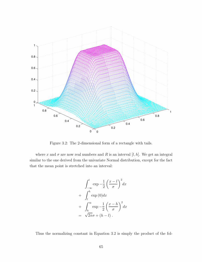
00.2

0.40.6

0.81

0

0.2

0.4

0.6

0.8

10

0.2

0.4

0.6

0.8

1

Figure 3.2: The 2-dimensional form of a rectangle with tails.

where x and σ are now real numbers and R is an interval [l, h]. We get an integral

similar to the one derived from the univariate Normal distribution, except for the fact

that the mean point is stretched into an interval:

∫ l

−∞exp−1

2

(

x− l

σ

)2

dx

+

∫ h

l

exp (0)dx

+

∫ ∞

h

exp−1

2

(

x− h

σ

)2

dx

=√

2πσ + (h− l) .

Thus the normalizing constant in Equation 3.2 is simply the product of the fol-

65

lowing per-dimension constants:

K−1 =M∏

d=1

[√2πσd + (Rh

d − Rld)]

.

Note the penalty imposed on high-volume rectangles. This will later prevent them

from expanding infinitely to try and capture all possible points.

3.2.2 Maximum Likelihood Estimation of a Single Tailed Rect-

angular Distribution

Suppose we have a dataset X = {x1, x2, . . . xR} and, given σ, we wish to find the

Maximum Likelihood (MLE) set of 2M parameters defining the rectangle. The log-

likelihood function is

LL(X) = (3.3)

∑

d

(

−R log(√

2πσd + Rhd − Rl

d)

+∑

i

−1

2

[

xid − closest(xi

d, Rld, R

hd))

σd

]2)

.

From this equation it is immediately clear that we can perform the MLE for each

dimension independently. For each dimension d in turn find the values l and h that

maximize

(

−R log(√

2πσ + h− l))

+∑

i

−1

2

[

xid − closest(xi

d, l, h)

σd

]2

.

We do this by first guessing an initial value of (l, h). Then we fix the low-point at l, and

find a good candidate for the new high boundary h′. Then we find a good candidate

for the low boundary l′ based on the existing h. Figure 3.3 shows an example of a

single fitting step for a single one-dimensional component. For each of the boundaries,

we want to maximize the likelihood which is a function of the new value. To achieve

this we use the golden-ratio one-dimensional optimizer (Press et al., 1992). Under the

assumption that the function is unimodal in the given range, this optimizer will find

a maximum point of it, up to the specified tolerance value. The number of function

evaluations is logarithmic in the width of the range. Although I have not yet proved

that the likelihood function is indeed unimodal, empirical evidence suggests this is

indeed the case.

66

3.2.3 EM Search for a Mixture of Tailed Rectangles

EM for mixture model clustering generally takes the following form:

1. Begin with a guess of the the mixture parameters {p1, θ1, p2, θ2, . . . pk, θk} where

pj is the probability of the mixture generating a data point from component j

and θj are the parameters for the j-th component. In our example θj consists of

2M parameters: the upper and lower bounds of the j-th rectangle. Note that

we are holding σ fixed during the iterations—we are not estimating it by EM.

2. For each data point xi and each mixture component j let wij be:

P (generated by j-th component | located atxi)

or, more succinctly,

wij = P (class = j | xi) .

This, by Bayes’ rule, is

wij =P (xi | class = j) · pj∑

l P (xi | class = l) · pl

.

3. For each component j, re-fit the parameters θj to a “weighted” version of the

dataset in which the i -th data point is given weight wij. Each data point thus

only counts as a fraction of a full data point in its contribution to the likelihood.

In our case this means we need to reestimate the coordinates of rectangle R = Rj

to maximize

LL(X) =

∑

d

(

−(∑

i

wij) log(√

2πσd + Rhd −Rl

d)

+∑

i

−wij

2

[

xid − closest(xi

d, Rld, R

hd)

σd

]2)

.

This can again be achieved one dimension at a time with two golden-ratio

searches per dimension: one for the lower and one for the upper bound.

67

3.2.4 The Full Algorithm

The full algorithm follows. Initialize the mixture components by taking, e.g. initial

points as used in the anchors hierarchy (Moore, 2000). Initialize σ (I currently use

some constant fraction of the range of the data in each dimension). For each dimension

and component, compute a new upper boundary based on the existing lower one, and

a new lower boundary, based on the current upper one. Change the boundaries and

iterate. Once stability is obtained, decrease σ (I multiply it by a constant factor

smaller than one) and continue iterating. Terminate if the components are all stable

immediately after decreasing σ.

3.2.5 Example

For illustration, Figures 3.4, 3.5, 3.6, 3.7 show runs on synthetic two-dimensional

datasets made by drawing points from component-wise rectangular distributions. Ini-

tially, the boundaries are quite arbitrary and σ is large. This allows the rectangles to

freely move to better locations. In following iterations, as σ decreases, the rectangles

try to reposition the boundaries to capture as many points as possible (since now the

penalty for excluding them is high). After a few more iterations, the distribution is

modeled accurately.

3.2.6 Intuition

Ultimately we are interested in obtaining a final mixture of hard rectangles (i.e.,

with infinitely steeply declining tails). But the key to the whole algorithm is the

use of relatively wider tails in the early stages. Without them, it is impossible for

rectangles to move because they would pay an infinite penalty for missing a single

data point with weight wij > 0. Thus, without the tails, the initial EM iterations see

all rectangles jump to the bounding box of the whole data, where they remain. It is

only with the tails that the rectangles are guided in directions to grow or shrink, and

are able to negotiate ownership of points with the other rectangles.


Our first test is as follows. Fix two parameters r and M . As usual, M is the

dimensionality of the data. Additionally, choose a set R ⊆ {1 . . .M} of r relevant

68

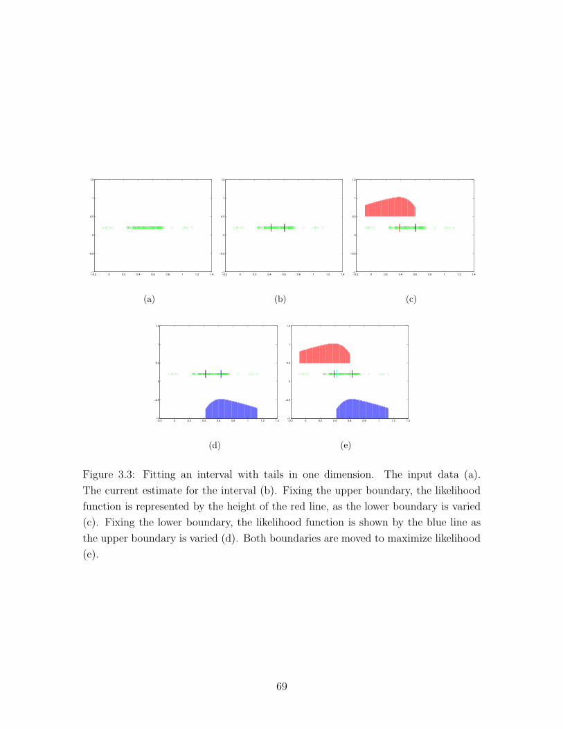
−0.2 0 0.2 0.4 0.6 0.8 1 1.2 1.4−1

−0.5

0

0.5

1

1.5

(a)

−0.2 0 0.2 0.4 0.6 0.8 1 1.2 1.4−1

−0.5

0

0.5

1

1.5

(b)

−0.2 0 0.2 0.4 0.6 0.8 1 1.2 1.4−1

−0.5

0

0.5

1

1.5

(c)

−0.2 0 0.2 0.4 0.6 0.8 1 1.2 1.4−1

−0.5

0

0.5

1

1.5

(d)

−0.2 0 0.2 0.4 0.6 0.8 1 1.2 1.4−1

−0.5

0

0.5

1

1.5

(e)

Figure 3.3: Fitting an interval with tails in one dimension. The input data (a).

The current estimate for the interval (b). Fixing the upper boundary, the likelihood

function is represented by the height of the red line, as the lower boundary is varied

(c). Fixing the lower boundary, the likelihood function is shown by the blue line as

the upper boundary is varied (d). Both boundaries are moved to maximize likelihood

(e).

69

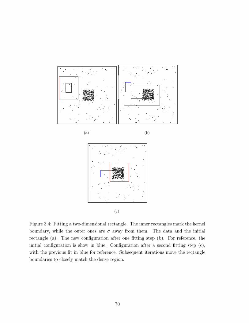
(a) (b)

(c)

Figure 3.4: Fitting a two-dimensional rectangle. The inner rectangles mark the kernel

boundary, while the outer ones are σ away from them. The data and the initial

rectangle (a). The new configuration after one fitting step (b). For reference, the

initial configuration is show in blue. Configuration after a second fitting step (c),

with the previous fit in blue for reference. Subsequent iterations move the rectangle

boundaries to closely match the dense region.

70

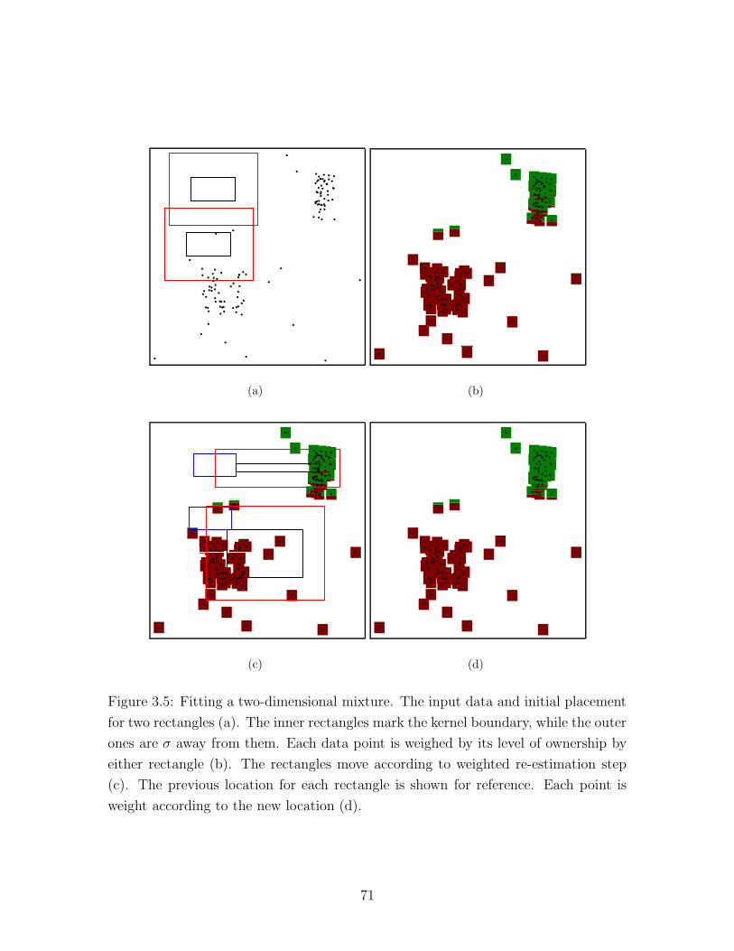
(a) (b)

(c) (d)

Figure 3.5: Fitting a two-dimensional mixture. The input data and initial placement

for two rectangles (a). The inner rectangles mark the kernel boundary, while the outer

ones are σ away from them. Each data point is weighed by its level of ownership by

either rectangle (b). The rectangles move according to weighted re-estimation step

(c). The previous location for each rectangle is shown for reference. Each point is

weight according to the new location (d).

71

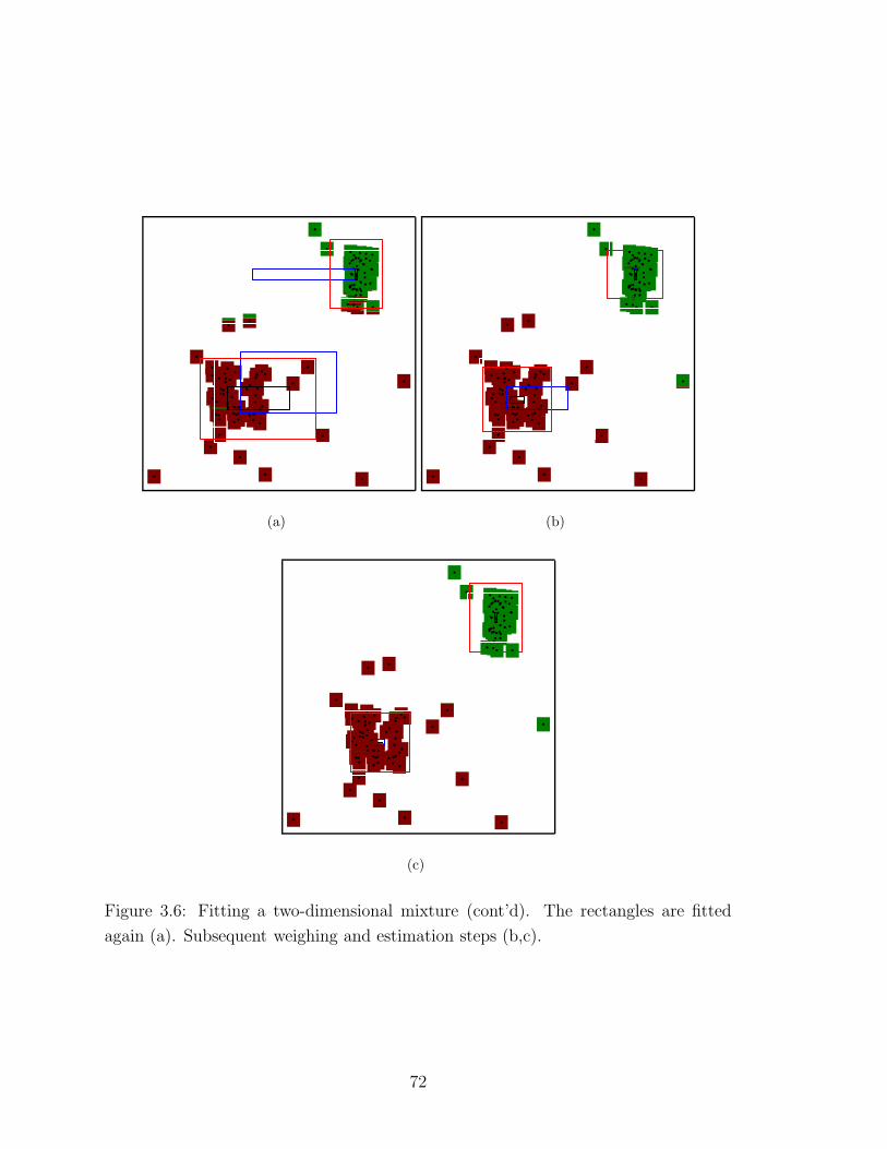
(a) (b)

(c)

Figure 3.6: Fitting a two-dimensional mixture (cont’d). The rectangles are fitted

again (a). Subsequent weighing and estimation steps (b,c).

72

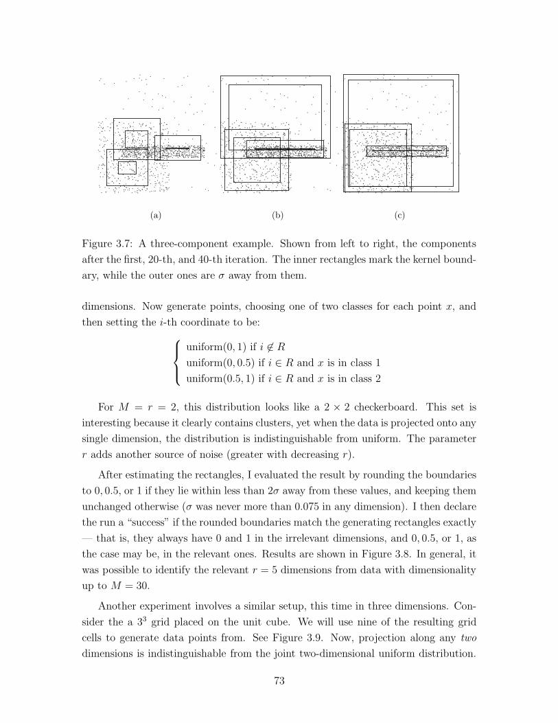
(a) (b) (c)

Figure 3.7: A three-component example. Shown from left to right, the components

after the first, 20-th, and 40-th iteration. The inner rectangles mark the kernel bound-

ary, while the outer ones are σ away from them.

dimensions. Now generate points, choosing one of two classes for each point x, and

then setting the i-th coordinate to be:

uniform(0, 1) if i 6∈ R

uniform(0, 0.5) if i ∈ R and x is in class 1

uniform(0.5, 1) if i ∈ R and x is in class 2

For M = r = 2, this distribution looks like a 2 × 2 checkerboard. This set is

interesting because it clearly contains clusters, yet when the data is projected onto any

single dimension, the distribution is indistinguishable from uniform. The parameter

r adds another source of noise (greater with decreasing r).

After estimating the rectangles, I evaluated the result by rounding the boundaries

to 0, 0.5, or 1 if they lie within less than 2σ away from these values, and keeping them

unchanged otherwise (σ was never more than 0.075 in any dimension). I then declare

the run a “success” if the rounded boundaries match the generating rectangles exactly

— that is, they always have 0 and 1 in the irrelevant dimensions, and 0, 0.5, or 1, as

the case may be, in the relevant ones. Results are shown in Figure 3.8. In general, it

was possible to identify the relevant r = 5 dimensions from data with dimensionality

up to M = 30.

Another experiment involves a similar setup, this time in three dimensions. Con-

sider the a 33 grid placed on the unit cube. We will use nine of the resulting grid

cells to generate data points from. See Figure 3.9. Now, projection along any two

dimensions is indistinguishable from the joint two-dimensional uniform distribution.

73

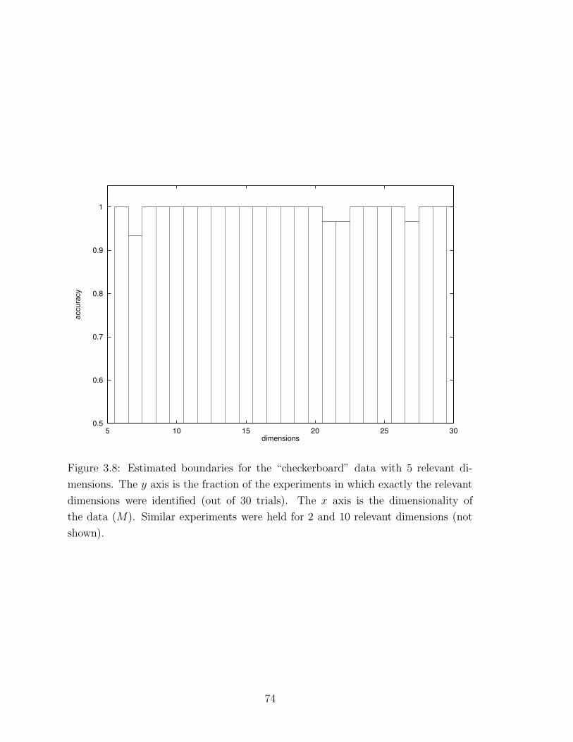
0.5

0.6

0.7

0.8

0.9

1

5 10 15 20 25 30

accu

racy

dimensions

Figure 3.8: Estimated boundaries for the “checkerboard” data with 5 relevant di-

mensions. The y axis is the fraction of the experiments in which exactly the relevant

dimensions were identified (out of 30 trials). The x axis is the dimensionality of

the data (M). Similar experiments were held for 2 and 10 relevant dimensions (not

shown).

74

Figure 3.9: Grid cells used for generation of data. Shown, from left to right, “slices”

along the third dimension, each of width 1/3.

Again, the estimated mixture is very close to the original one, as seen in Figure 3.10.

In another experiment, data points were generated from a mixture as follows. In

each dimension, a random interval with expected width 0.4 was drawn from [0, 1].

The intersection of these intervals defines a hyper-rectangle, and data points were

generated from the union of several such components. The estimated distribution was

evaluated as follows. Fix a mapping from the true distribution to the estimated one.

Each estimated rectangle is compared to the matching true rectangle by taking the

M -th root of the ratio between the volumes of the intersection of the two rectangles to

their union. The similarity of the two distributions is just the average of these values,

taken over all rectangle pairs. The values reported here are the maximum similarity

values taken over all possible mappings (i.e., all permutations over [1, . . . k], where

k is the number of components). See Figure 3.11. The results show that generally

similarity of in the 90% range.

I have also performed sporadic experiments to test the sensitivity of the algorithm

to the different parameters. Figure 3.12 shows how supplying the wrong number

of rectangles might affect the run. Another parameter is the initial value for σ. I

currently use a rather simplistic estimate of 1/10 of the range of the input. It does

work for my datasets. A more sophisticated approach would be to first try and

estimate σ (say, using a model with spherical Gaussians) and use the estimate to set

the rectangle tails.

Experiments on real-life data were done on the “mpg” and “census” datasets from

the UCI repository (Blake & Merz, 1998). The “mpg” data has about 400 records

with 7 continuous2 attributes. Running on this data with the number of components

set to three, we get the results shown in Table 3.1. Interpreting this data, we see that

cars with at most four cylinders are the most economical, and that eight-cylinder cars

2We treat discrete attributes as continuous if the values can be linearly ordered (e.g., number of

cylinders and model year).

75

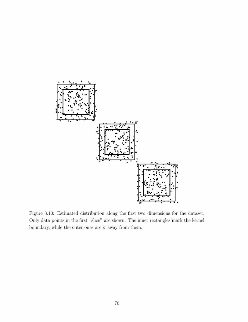
Figure 3.10: Estimated distribution along the first two dimensions for the dataset.

Only data points in the first “slice” are shown. The inner rectangles mark the kernel

boundary, while the outer ones are σ away from them.

76

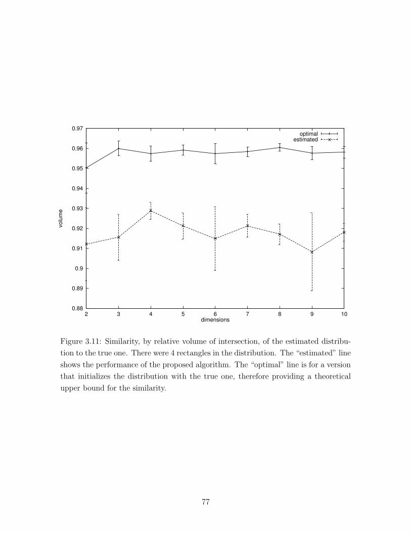
0.88

0.89

0.9

0.91

0.92

0.93

0.94

0.95

0.96

0.97

2 3 4 5 6 7 8 9 10

volu

me

dimensions

optimalestimated

Figure 3.11: Similarity, by relative volume of intersection, of the estimated distribu-

tion to the true one. There were 4 rectangles in the distribution. The “estimated” line

shows the performance of the proposed algorithm. The “optimal” line is for a version

that initializes the distribution with the true one, therefore providing a theoretical

upper bound for the similarity.

77

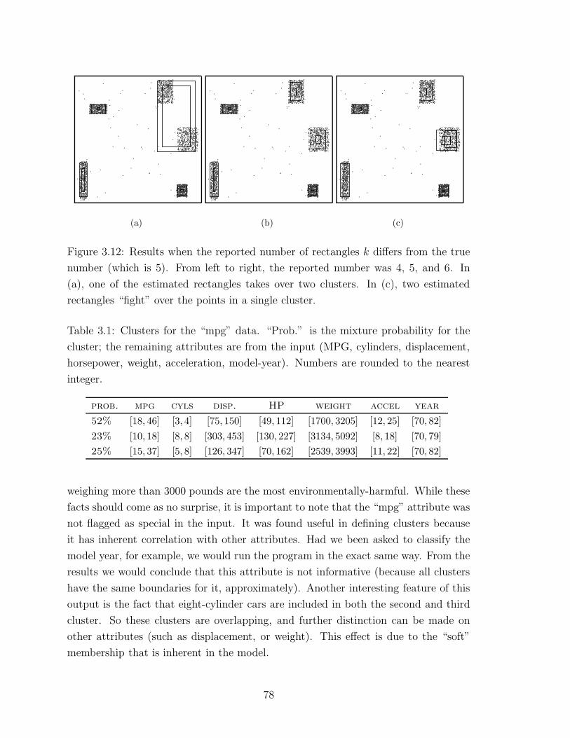
(a) (b) (c)

Figure 3.12: Results when the reported number of rectangles k differs from the true

number (which is 5). From left to right, the reported number was 4, 5, and 6. In

(a), one of the estimated rectangles takes over two clusters. In (c), two estimated

rectangles “fight” over the points in a single cluster.

Table 3.1: Clusters for the “mpg” data. “Prob.” is the mixture probability for the

cluster; the remaining attributes are from the input (MPG, cylinders, displacement,

horsepower, weight, acceleration, model-year). Numbers are rounded to the nearest

integer.

prob. mpg cyls disp. HP weight accel year

52% [18, 46] [3, 4] [75, 150] [49, 112] [1700, 3205] [12, 25] [70, 82]

23% [10, 18] [8, 8] [303, 453] [130, 227] [3134, 5092] [8, 18] [70, 79]

25% [15, 37] [5, 8] [126, 347] [70, 162] [2539, 3993] [11, 22] [70, 82]

weighing more than 3000 pounds are the most environmentally-harmful. While these

facts should come as no surprise, it is important to note that the “mpg” attribute was

not flagged as special in the input. It was found useful in defining clusters because

it has inherent correlation with other attributes. Had we been asked to classify the

model year, for example, we would run the program in the exact same way. From the

results we would conclude that this attribute is not informative (because all clusters

have the same boundaries for it, approximately). Another interesting feature of this

output is the fact that eight-cylinder cars are included in both the second and third

cluster. So these clusters are overlapping, and further distinction can be made on

other attributes (such as displacement, or weight). This effect is due to the “soft”

membership that is inherent in the model.

78

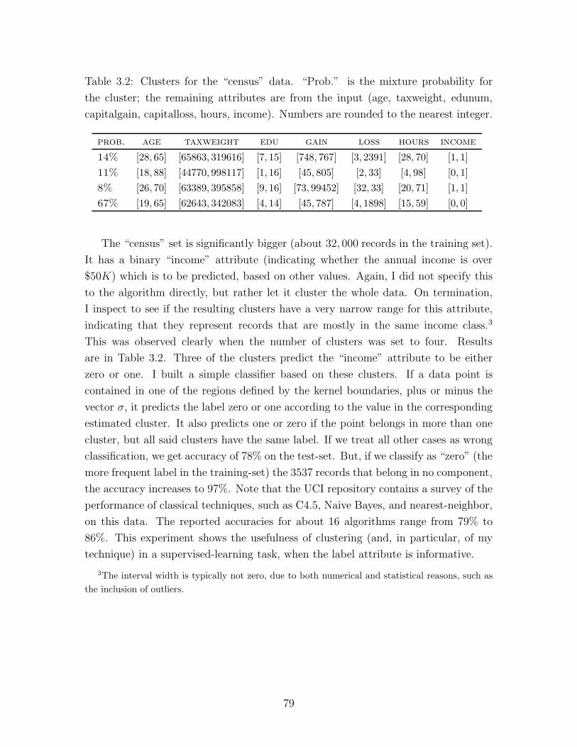
Table 3.2: Clusters for the “census” data. “Prob.” is the mixture probability for

the cluster; the remaining attributes are from the input (age, taxweight, edunum,

capitalgain, capitalloss, hours, income). Numbers are rounded to the nearest integer.

prob. age taxweight edu gain loss hours income

14% [28, 65] [65863, 319616] [7, 15] [748, 767] [3, 2391] [28, 70] [1, 1]

11% [18, 88] [44770, 998117] [1, 16] [45, 805] [2, 33] [4, 98] [0, 1]

8% [26, 70] [63389, 395858] [9, 16] [73, 99452] [32, 33] [20, 71] [1, 1]

67% [19, 65] [62643, 342083] [4, 14] [45, 787] [4, 1898] [15, 59] [0, 0]

The “census” set is significantly bigger (about 32, 000 records in the training set).

It has a binary “income” attribute (indicating whether the annual income is over

$50K) which is to be predicted, based on other values. Again, I did not specify this

to the algorithm directly, but rather let it cluster the whole data. On termination,

I inspect to see if the resulting clusters have a very narrow range for this attribute,

indicating that they represent records that are mostly in the same income class.3

This was observed clearly when the number of clusters was set to four. Results

are in Table 3.2. Three of the clusters predict the “income” attribute to be either

zero or one. I built a simple classifier based on these clusters. If a data point is

contained in one of the regions defined by the kernel boundaries, plus or minus the

vector σ, it predicts the label zero or one according to the value in the corresponding

estimated cluster. It also predicts one or zero if the point belongs in more than one

cluster, but all said clusters have the same label. If we treat all other cases as wrong

classification, we get accuracy of 78% on the test-set. But, if we classify as “zero” (the

more frequent label in the training-set) the 3537 records that belong in no component,

the accuracy increases to 97%. Note that the UCI repository contains a survey of the

performance of classical techniques, such as C4.5, Naive Bayes, and nearest-neighbor,

on this data. The reported accuracies for about 16 algorithms range from 79% to

86%. This experiment shows the usefulness of clustering (and, in particular, of my

technique) in a supervised-learning task, when the label attribute is informative.

3The interval width is typically not zero, due to both numerical and statistical reasons, such as

the inclusion of outliers.

79

3.4 Conclusion

I have demonstrated a method that benefits from the usefulness of soft membership

and the expressiveness and clean analysis of mixture models. At the same time,

the produced clusters have a compact representation which people can find compre-

hensible. As an added bonus, expanding the Gaussian means into a rectangular form

seems to help avoid the inherent statistical problems that come with high-dimensional

distance computations. The resulting clusters are highly readable and allow for the

construction of very simple, yet very effective, classifiers. The proposed model was

also shown to be effective in dimension-reduction tasks.

My implementation has been used to visualize highway traffic data (Raz et al.,

2004). Truck weigh-in-motion data collected by the Minnesota department of trans-

portation was analyzed with a variety of methods and presented to a domain expert.

The mixture of rectangles was reported to produce crisp models and made it easy to

point out the anomalies. For example, a common misclassification failure was detected

where the low-level software would determine some trucks had one axle. Another ob-

servation made clear was a system-wide change around November 1999. Later it

was discovered that a vendor of one of the software components made unreported

configuration changes at that date.

I believe it would be straightforward to extend this method to data involving

discrete attributes. For a given mixture component, each discrete attribute would be

modeled independently by a multinomial distribution. The parameters needed for an

n-ary attribute would simply be the n multinomial probabilities (which must sum to

one). In the case of all-discrete (i.e., no real-valued) attributes, this would degenerate

to the well-known mixtures of products of multinomials distribution (e.g. Meila and

Heckerman (1998)).

A natural extension would be to get rid of the single parameter that the user needs

to supply — the desired number of clusters. Ideally the algorithm would estimate

this by itself.

I argue that the representation of clusters as intersection of intervals is succinct.

However, there is room for improvement, especially if the data dimensionality is very

large. I believe that a post-processing step that identifies the irrelevant dimensions

and removes them from the output can be easily implemented. Another useful oper-

ation would be to sort the dimensions by their “importance” (or contribution to the

log-likelihood) before presenting the intervals.

80

Chapter 4

Fast Dependency Tree

Construction

We continue our quest to find useful models. Bayesian networks are a popular class

of very general models. They are also appealing from the cognitive aspect as their

structure — if not too complex — can often be visualized and easily understood.

However, they are hard to fit from data because of their richness.

I am interested in restricting the search space by considering only a simpler sub-

class of graphical models, namely trees. For trees, a well-known algorithm can find

optimal solutions in polynomial time. As an added feature, the trees can be described

more simply to human users. I show how to accelerate the known algorithm to run

in sub-linear time. Empirical evidence shows run time which is linear in the number

of attributes, and constant regardless in the input size. The constant depends only

on intrinsic properties of the data. This allows processing of very large data sets.

4.1 Introduction

Bayes nets are widely used for data modeling. However, the problem of constructing

Bayes nets from data remains a hard one, requiring search in a super-exponential

space of possible graph structures. Despite recent advances (Friedman et al., 1999),

learning network structure from big data sets demands huge computational resources.

We therefore turn to a simpler model, which is easier to compute while still being

expressive enough to be useful. Namely, we look at dependency trees, which are

belief networks that satisfy the additional constraint that each node has at most one

parent. In this simple case it has been shown (Chow & Liu, 1968) that finding the

81

tree that maximizes the data likelihood can be reduced to a much simpler problem.

First, construct a full graph where each node corresponds to an attribute in the input

data. Next, assign edge weights; these are are derived from the mutual information

values of the corresponding attribute pairs. Finally, run a minimum1 spanning tree

algorithm on the weighted graph. The output tree is the desired one.

Dependency trees are interesting in their own right. They form a complete repre-

sentation. Additionally they can act as initializers for search, as mixture components

(Meila, 1999b), or as components in classifiers (Friedman et al., 1998). It is my intent

to eventually apply the technology introduced here to the full problem of Bayes Net

structure search.

Once the weight matrix is constructed, executing a minimum spanning tree (MST)

algorithm is fast. The time-consuming part is the population of the weight matrix,

which takes time O(RM 2). This becomes expensive when considering datasets with

hundreds of thousands of records (R) and hundreds of attributes (M).

To overcome this problem, I propose a new way of interleaving the spanning

tree construction with the operations needed to compute the mutual information

coefficients. I develop a new spanning-tree algorithm, based solely on Tarjan’s (1983)

red-edge rule. This algorithm is capable of using partial knowledge about edge weights

and of signaling the need for more accurate information regarding a particular edge.

The partial information we maintain is in the form of probabilistic confidence intervals

on the edge weights; an interval is derived by looking at a sub-sample of the data for

a particular attribute pair. Whenever the algorithm signals that a currently-known

interval is too wide, we inspect more data records in order to shrink it. Once the

interval is small enough, we may be able to prove that the corresponding edge is not

a part of the tree. Whenever such an edge can be eliminated without looking at the

full data set, the work associated with the remainder of the data is saved. This is

where performance is gained.

I have implemented the algorithm for numeric and categorical data and tested

it on real and synthetic data sets containing hundreds of attributes and millions of

records. I show experimental results of up to 5,000-fold speed improvements over the

traditional algorithm. The resulting trees are, in most cases, of near-identical quality

to the ones grown by the naive algorithm.

Use of probabilistic bounds to direct structure-search appears in Maron and Moore

1To be precise, we will use it as a maximum spanning tree algorithm. The two are interchangeable,

requiring just a reversal of the edge weight comparison operator. Historically, minimum has been

far more popular a name.

82

(1994) for classification and in Moore and Lee (1994) for model selection. In a se-

quence of papers, Domingos et al. have demonstrated the usefulness of this technique

for decision trees (Domingos & Hulten, 2000), K-means clustering (Domingos & Hul-

ten, 2001a), and mixtures-of-Gaussians EM (Domingos & Hulten, 2001b). In the

context of dependency trees, Meila (1999a) discusses the discrete case that frequently

comes up in text-mining applications, where the attributes are sparse in the sense

that only a small fraction of them are true for any record. In this case it is possible

to exploit the sparseness and accelerate the Chow-Liu algorithm.

Throughout the chapter we use the following notation. The number of data records

is R, the number of attributes M . When x is an attribute, xi is the value it takes

for the i-th record. We denote by ρxy the correlation coefficient between attributes x

and y, and omit the subscript when it is clear from the context. Hx is the entropy of

an attribute or an attribute set x.

4.2 A Slow Minimum-Spanning Tree Algorithm

We begin by describing our MST algorithm. Although in its given form it can be

applied to any graph, it is asymptotically slower than established algorithms (as

predicted in Tarjan (1983) for all algorithms in its class). We then proceed to describe

its use in the case where some edge weights are known not exactly, but rather only

to lie within a given interval. In Section 4.4 we will show how this property of the

algorithm interacts with the data-scanning step to produce an efficient dependency-

tree algorithm.

In the following discussion we assume we are given a complete graph with n nodes,

and the task is to find a tree connecting all of its nodes such that the total tree weight

(defined to be the sum of the weights of its edges) is minimized. This problem has

been extremely well studied and numerous efficient algorithms for it exist.

We start with a rule to eliminate edges from consideration for the output tree.

Following Tarjan (1983), we state the so-called “red-edge” rule:

Theorem 7: The heaviest edge in any cycle in the graph is not part of the minimum

spanning tree.

Traditionally, MST algorithms use this rule in conjunction with a greedy “blue-

edge” rule, which chooses edges for inclusion in the tree. In contrast, we will repeat-

edly use the red-edge rule until all but n− 1 edges have been eliminated. The proof

this results in a minimum-spanning tree follows from Tarjan (1983).

83

Let E be the original set of edges. Denote by L the set of edges that have already

been eliminated, and let L = E \ L. As a way to guide our search for edges to

eliminate we maintain the following invariant:

Invariant 8: At any point there is a spanning tree T , which is composed of edges

in L.

In each step, we arbitrarily choose some edge e in L \ T and try to eliminate it

using the red-edge rule. Recall that the rule needs a cycle to act on. Let P be the

path in T between e’s endpoints. The cycle we will apply the red-edge rule to will

be composed of e and P . It is clear we only need to compare e with the heaviest

edge in P . If e is heavier, we can eliminate it by the red-edge rule. However, if it is

lighter, then we can eliminate the tree edge by the same rule. If this is indeed the

case, we do so and add e to the tree to preserve Invariant 8. The algorithm, which

we call Minimum Incremental Spanning Tree (MIST), is listed in Figure 4.1. Figures

4.2,4.3,4.4 and 4.5 illustrate how it may run on an example graph.

The MIST algorithm can be applied directly to a graph where the edge weights

are known exactly. And like many other MST algorithms, it can also be used in the

case where just the relative order of the edge weights is given. Now imagine a different

setting, where edge weights are not given, and instead an oracle exists, who knows

the exact values of the edge weights. When asked about the relative order of two

edges, it may either respond with the correct answer, or it may give an inconclusive

answer. Furthermore, a constant fee is charged for each query. In this setup, MIST is

still suited for finding a spanning tree while minimizing the number of queries issued.

In step 2, we go to the oracle to determine the order. If the answer is conclusive, the

algorithm proceeds as described. Otherwise, it just ignores the “if” clause altogether

and iterates (possibly with a different edge e).

For the moment, this setting may seem contrived, but in Section 4.4, we go back

to the MIST algorithm and put it in a context very similar to the one described here.

4.3 Probabilistic Bounds on Mutual Information

We now concentrate once again on the specific problem of determining the mutual

information between a pair of attributes. We show how to compute it given the

complete data, and how to derive probabilistic confidence intervals for it, given just

a sample of the data.

84

1. T ← an arbitrary spanning set of n− 1 edges.

L← empty set.

2. While |L| > n− 1 do:

Pick an arbitrary edge e ∈ L \ T .

Let e′ be the heaviest edge on the path in T between the

endpoints of e.

If e is heavier than e′:

L← L ∪ {e}otherwise:

T ← T ∪ {e} \ {e′}L← L ∪ {e′}

3. Output T .

Figure 4.1: The MIST algorithm. At each step of the iteration, T contains the current

“draft” tree. L contains the set of edges that have been proven to not be in the MST

and so L contains the set of edges that still have some chance of being in the MST.

T never contains an edge in L.

85

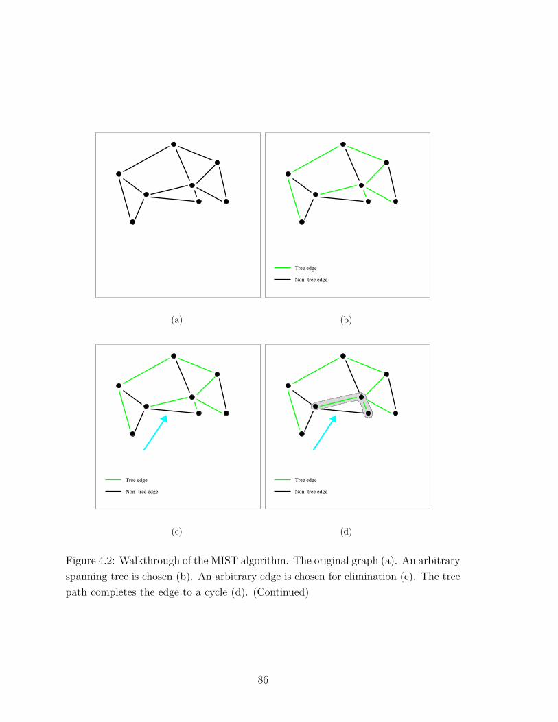
(a)

Non−tree edge

Tree edge

(b)

Tree edge

Non−tree edge

(c)

Tree edge

Non−tree edge

(d)

Figure 4.2: Walkthrough of the MIST algorithm. The original graph (a). An arbitrary

spanning tree is chosen (b). An arbitrary edge is chosen for elimination (c). The tree

path completes the edge to a cycle (d). (Continued)

86

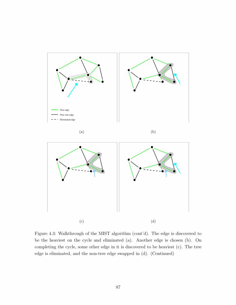
Tree edge

Non−tree edge

Eliminated edge

(a) (b)

(c) (d)

Figure 4.3: Walkthrough of the MIST algorithm (cont’d). The edge is discovered to

be the heaviest on the cycle and eliminated (a). Another edge is chosen (b). On

completing the cycle, some other edge in it is discovered to be heaviest (c). The tree

edge is eliminated, and the non-tree edge swapped in (d). (Continued)

87

(a) (b)

(c) (d)

Figure 4.4: Walkthrough of the MIST algorithm (cont’d). The updated tree (a). An-

other edge is chosen (b). The tree cycle is completed and the non-tree edge eliminated

(c). The next edge is chosen (d). (Continued)

88

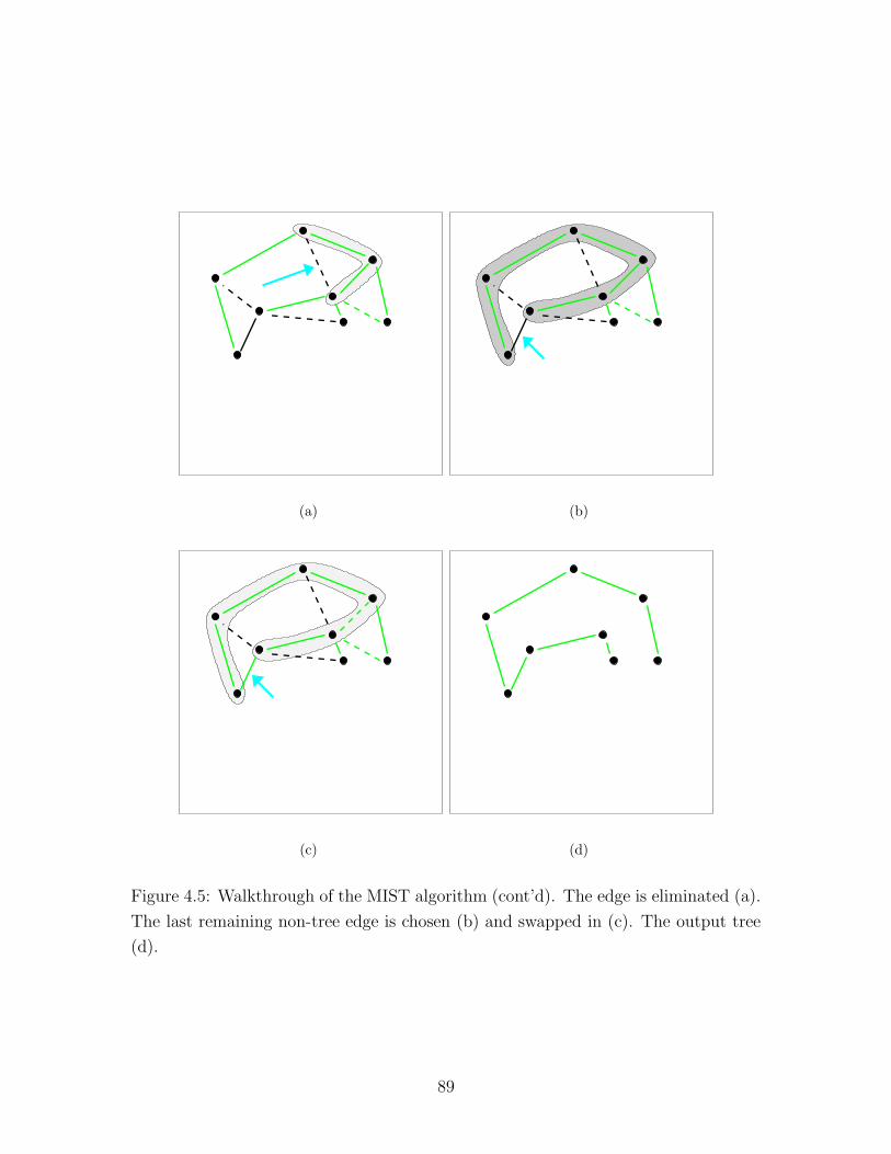
(a) (b)

(c) (d)

Figure 4.5: Walkthrough of the MIST algorithm (cont’d). The edge is eliminated (a).

The last remaining non-tree edge is chosen (b) and swapped in (c). The output tree

(d).

89

As shown in (Reza, 1994), the mutual information for two jointly Gaussian numeric

attributes X and Y is:

I(X; Y ) = −1

2ln(1− ρ2)

where the correlation coefficient ρ = ρXY =

∑Ri=1 ((xi − x)(yi − y))

σ2X σ2

Y

with x, y, σ2X and σ2

Y being the sample means and variances for attributes X and Y .

In practice, we standardize the data in a pre-processing step to have zero mean and

unit variance. This leaves xi · yi as the only unknown.

Since the log function is monotonic, I(X; Y ) is also monotonic in |ρ|. This is a

sufficient condition for the use of |ρ| as the edge weight in a MST algorithm. Con-

sequently, the sample correlation can be used in a straightforward manner when the

complete data is available. Now consider the case where just a sample of the data

has been observed.

Let x and y be two data attributes. We are trying to estimate∑R

i=1 xi · yi given

the partial sum∑r

i=1 xi · yi for some r < R. To derive a confidence interval, we use

the Central Limit Theorem.2 It states that given samples of the random variable

Z (where for our purposes Zi = xi · yi), the sum∑

i Zi can be approximated by a

Normal distribution with mean and variance closely related to the distribution mean

and variance. Furthermore, for large samples, the sample mean and variance can

be substituted for the unknown distribution parameters. Note in particular that the

central limit theorem does not require us to make any assumption about the Gaus-

sianity of Z. We thus can derive a two-sided confidence interval for∑

i Zi =∑

i xi ·yi

with probability 1 − δ for some user-specified δ, typically 1%. Given this interval,

computing an interval for ρ is straightforward.

2One can use the weaker Hoeffding bound instead, and my implementation supports it as well,

although it is generally much less powerful.

90

In the case of binary categorical data, we follow Meila (1999b) and write:

I(X; Y ) = HX + HY −HXY

=1

R[−zlogz(NX)− zlogz(N −NX)

− zlogz(NY )− zlogz(N −NY )

+ zlogz(NXY ) + zlogz(NX −NXY )

+ zlogz(NY −NXY )

+ zlogz(R−NX −NY + NXY )

+ zlogz(R)] (4.1)

where zlogz(z) is shorthand for z log z and Nz denotes the number of times an

attribute or a set of attributes are observed all true. As before, NXY is the quantity

we are deriving a probabilistic estimate for, which we do from the counts in a sample

and application of the CLT.

Now, observe that:

d(zlogz(y))/dx = dy log y/dx

= dy/dx log y + y · 1y· dy/dx

= (1 + log y)dy/dx .

We take a derivative of I(X; Y ) with respect to measured quantity NXY . The

only terms in 4.1 which do not zero out are the ones containing NXY .

d(I(X; Y ))/dNxy = (1 + log Nxy)− (1 + log (Nx −Nxy))

−(1 + log (Ny −Nxy)) + (1 + log (R−Nx −Ny + Nxy))

= log Nxy − log (Nx −Nxy)− log (Ny −Nxy) + log (R−Nx −Ny + Nxy) =

= logNxy(R−Nx + Ny + Nxy)

(Nx −Nxy)(Ny −Nxy). (4.2)

Let Nxy be the number of records for which both attributes were false, and simi-

larly for Nxy and Nxy. Immediately we get:

Nxy = Nx −Nxy

Nxy = Ny −Nxy

Nxy = R−Nx + Ny + Nxy .

91

Then, equality with zero in Equation 4.2 above is obtained when:

NxyNxy = NxyNxy

or:

Nxy =NxyNxy

Nxy(4.3)

Therefore, to determine minimum and maximum values for I(X; Y ) at the interval,

we evaluate it at the endpoints. Additionally, we evaluate at the extreme point if it

happens to be included in the interval.

4.4 The Full Algorithm

As we argued, the MIST algorithm is capable of using partial information about edge

weights. We have also shown how to derive confidence intervals on edge weights. We

now combine the two and give an efficient dependency-tree algorithm.

We largely follow the MIST algorithm as listed in Figure 4.1. We initialize the

tree T in the following heuristic way: first we take a small sub-sample of the data,

and derive point estimates for the edge weights from it. Then feed the point estimates

to any MST algorithm and obtain a tree T .

When we come to compare edge weights, we generally need to deal with two

intervals. If they do not intersect, then the points in one of them are all smaller in

value than any point in the other, in which case we can determine which represents a

heavier edge. We apply this logic to all comparisons, where the goal is to determine

the heaviest path edge e′ and to compare it to the candidate e. If we are lucky enough

that all of these comparisons are conclusive, the amount of work we save is related

to how much data was used in computing the confidence intervals — the rest of the

data for the attribute-pair that is represented by the eliminated edge can be ignored.

However, there is no guarantee that the intervals are separated and allow us to

draw meaningful conclusions. If they do not, then we have a situation similar to the

inconclusive oracle answers in Section 4.2. The price we need to pay here is looking

at more data to shrink the confidence intervals. We do this by choosing one edge —

either a tree-path edge or the candidate edge — for “promotion”, and doubling the

sample size used to compute the sufficient statistics for it. After doing so we try to

eliminate again (since we can do this at no additional cost). If we fail to eliminate

we iterate, possibly choosing a different candidate edge (and the corresponding tree

path) this time.

92

The choice of which edge to promote is heuristic, and depends on the expected

success of resolution once the interval has shrunk. This is estimated by first defining

a cost measure for a set of tree edges and a candidate edge. It is the sum of the sizes

of intersections of the tree edges with the candidate edge, plus the size of intersections

between the worst tree edge (as defined by the mid-points of the intervals) and the

other tree edges. We now go over the tree edges, in turn, and for each one estimate

the size of its interval, if given more data. This estimate depends on the measured

variance in the observed data. We record the cost for each of these speculative edges.

The one associated with the lowest cost is chosen, unless the expected difference from

the current cost is below a threshold. If this holds, we pick an edge at random from the

set of edges that define the boundary of the union of the tree edges which intersects

with the candidate edge. If this is impossible (for example, all of these edges are

already saturated), we choose some tree-path edge at random.

Another heuristic we employ goes as follows. Consider the comparison of the path-

heaviest edge to an estimate of a candidate edge. The interval for the candidate edge

may be very small, and yet still intersect the interval that is the heavy edge’s weight

(this would happen if, for example, both attribute-pairs have the same distribution).

We may be able to reduce the amount of work by pretending the interval is narrower

than it really is. We therefore trim the interval by a constant, parameterized by the

user as ε, before performing the comparison. This use of δ and ε is analogous to

their use in “Probably Approximately Correct” analysis: on each decision, with high

probability (1− δ) we will make at worst a small mistake (ε).

4.4.1 Algorithm Complexity

We now discuss the theoretical complexity of the proposed algorithm. Refer to Fig-

ure 4.1. In theory, the first step can be done by choosing edges at random. In practice,

it is built by sampling some number S of records from the input, and running a Chow-

Liu algorithm on the sample. The complexity of obtaining the sample is O(SM 2). If

M is very large then this can dominate the run time. A possible countermeasure is

to choose S proportional to M−2. However this is not always possible: if M 2 is in the

order of R or greater, this will result in a sample size smaller than one. Therefore the

worst case time here is O(M 2). Finding the actual minimum spanning tree on the

sample can be done in time O(M 2 + M log M) by Prim’s algorithm using Fibonacci

heaps (Cormen et al., 1989).

Step 2 in Figure 4.1 requires O(M 2) successful elimination steps. Each step re-

93

quires, aside from the work required to read more data, finding a tree path between

two nodes. In the worst case, this can take O(M) work since the current tree contains

M − 1 edges. Therefore the cost for this step is O(M 3). It is possible that the cost of

finding and updating tree paths can be amortized (Tarjan, 1983). But more impor-

tantly, elimination of tree edges is a rare occurrence, so the tree structure is generally

static. Therefore tree paths can be recorded and re-used instead of discovered. This

is done in the current implementation.

Below, I present empirical results showing that the worst case is an overestimate

for the data sets in question. In particular Figure 4.7 shows that for synthetic sets

with M < 160, performance is still comfortably in the linear range.


In the following description of experiments, we vary different parameters for the data

and the algorithm. Unless otherwise specified, here are the default values for the

parameters. We set δ to 1% and ε to 0.05 (on either side of the interval, totaling 0.1).

The initial sample size is fifty records. There are 100, 000 records and 100 attributes.

The data is real-valued. The data-generation process first generates a random tree,

then draws points for each node from a normal distribution with the node’s parent’s

value as the mean. In addition, any data value is set to random noise with probability

0.15.

To construct the correlation matrix from the full data, each of the R records needs

to be considered for each of the(

M2

)

attribute pairs. We evaluate the performance

of our algorithm by adding the number of records that were actually scanned for all

the attribute-pairs, and dividing the total by R(

M2

)

. We call this number the “data

usage” of our algorithm. The closer it is to zero, the more efficient our sampling is,

while a value of one means the same amount of work as for the full-data algorithm

(possibly more, when considering the overhead).

We first demonstrate the speed of our algorithm as compared with the full O(RM 2)

scan. Figure 4.6 shows that the amount of data the algorithm examines is a constant

that does not depend on the size of the data set. This translates to relative run-

times of 0.7% (for the 37, 500-record set) to 0.02% (for the 1, 200, 000-record set) as

compared with the full-data algorithm. The latter number translates to a 5, 000-fold

speedup. Note that the reported usage is an average over the number of attributes.

However this does not mean that the same amount of data was inspected for every

attribute-pair — the algorithm determines how much effort to invest in each edge

94

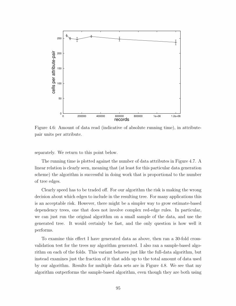
0

50

100

150

200

250

0 200000 400000 600000 800000 1e+06 1.2e+06

cells

per

attr

ibut

e-pa

ir

records

Figure 4.6: Amount of data read (indicative of absolute running time), in attribute-

pair units per attribute.

separately. We return to this point below.

The running time is plotted against the number of data attributes in Figure 4.7. A

linear relation is clearly seen, meaning that (at least for this particular data generation

scheme) the algorithm is successful in doing work that is proportional to the number

of tree edges.

Clearly speed has to be traded off. For our algorithm the risk is making the wrong

decision about which edges to include in the resulting tree. For many applications this

is an acceptable risk. However, there might be a simpler way to grow estimate-based

dependency trees, one that does not involve complex red-edge rules. In particular,

we can just run the original algorithm on a small sample of the data, and use the

generated tree. It would certainly be fast, and the only question is how well it

performs.

To examine this effect I have generated data as above, then ran a 30-fold cross-

validation test for the trees my algorithm generated. I also ran a sample-based algo-

rithm on each of the folds. This variant behaves just like the full-data algorithm, but

instead examines just the fraction of it that adds up to the total amount of data used

by our algorithm. Results for multiple data sets are in Figure 4.8. We see that my

algorithm outperforms the sample-based algorithm, even though they are both using

95

0

5

10

15

20

25

30

20 40 60 80 100 120 140 160

runn

ing

time

number of attributes

Figure 4.7: Running time as a function of the number of attributes.

0

0.5

1

1.5

2

0 200000 400000 600000 800000 1e+06 1.2e+06

rela

tive

log-

likel

ihoo

d

records

Figure 4.8: Relative log-likelihood vs. the sample-based algorithm. The log-likelihood

difference is divided by the number of records.

96

-6

-5

-4

-3

-2

-1

0

0.001 0.0015 0.002 0.0025 0.003 0.0035 0.004

rela

tive

log-

likel

ihoo

d

data usage

MISTSAMPLE

Figure 4.9: Relative log-likelihood vs. the sample-based algorithm, drawn against the

fraction of data scanned.

the same total amount of data. The reason is that using the same amount of data for

all edges assumes all attribute-pairs have the same variance. This is in contrast to my

algorithm, which determines the amount of data for each edge independently. Appar-

ently for some edges this decision is very easy, requiring just a small sample. These

“savings” can be used to look at more data for high-variance edges. The sample-

based algorithm would not put more effort into those high-variance edges, eventually

making the wrong decision. In Figure 4.9 I show the log-likelihood difference for a

particular (randomly generated) set. Here, multiple runs with different δ and ε values

were performed, and the result is plotted against the fraction of data used. The base-

line (0) is the log-likelihood of the tree grown by the original algorithm using the full

data. Again we see that MIST is better over a wide range of data utilization ratios.

Keep in mind that the sample-based algorithm has been given an unfair advantage,

compared with MIST: it knows how much data it needs to look at. This parameter

is implicitly passed to it from my algorithm, and represents an important piece of

information about the data. Without it, there would need to be a preliminary stage

to determine the sample size. The alternative is to use a fixed amount (specified

either as a fraction or as an absolute count), which is likely to be too much or too

little. Another option is to iterate over increasing data sizes (for example, double the

sample size in each iteration). The problem with this approach is that it still leaves

97

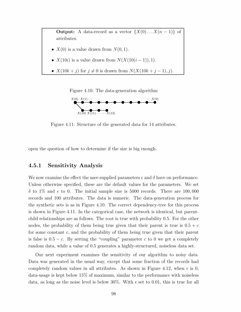
Output: A data-record as a vector {X(0) . . .X(n − 1)} of

attributes.

• X(0) is a value drawn from N(0, 1).

• X(10i) is a value drawn from N(X(10(i− 1)), 1).

• X(10k + j) for j 6= 0 is drawn from N(X(10k + j − 1), j).

Figure 4.10: The data-generation algorithm

· · ·X(13)X(11) · · ·

X(0) X(1) · · · · · ·X(9)

X(10)

Figure 4.11: Structure of the generated data for 14 attributes.

open the question of how to determine if the size is big enough.

4.5.1 Sensitivity Analysis

We now examine the effect the user-supplied parameters ε and δ have on performance.

Unless otherwise specified, these are the default values for the parameters. We set

δ to 1% and ε to 0. The initial sample size is 5000 records. There are 100, 000

records and 100 attributes. The data is numeric. The data-generation process for

the synthetic sets is as in Figure 4.10. The correct dependency-tree for this process

is shown in Figure 4.11. In the categorical case, the network is identical, but parent-

child relationships are as follows. The root is true with probability 0.5. For the other

nodes, the probability of them being true given that their parent is true is 0.5 + c

for some constant c, and the probability of them being true given that their parent

is false is 0.5 − c. By setting the “coupling” parameter c to 0 we get a completely

random data, while a value of 0.5 generates a highly-structured, noiseless data set.

Our next experiment examines the sensitivity of our algorithm to noisy data.

Data was generated in the usual way, except that some fraction of the records had

completely random values in all attributes. As shown in Figure 4.12, when ε is 0,

data-usage is kept below 15% of maximum, similar to the performance with noiseless

data, as long as the noise level is below 30%. With ε set to 0.01, this is true for all

98

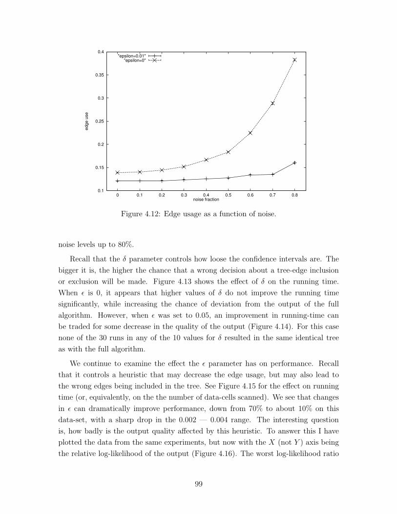
0.1

0.15

0.2

0.25

0.3

0.35

0.4

0 0.1 0.2 0.3 0.4 0.5 0.6 0.7 0.8

edge

use

noise fraction

"epsilon=0.01""epsilon=0"

Figure 4.12: Edge usage as a function of noise.

noise levels up to 80%.

Recall that the δ parameter controls how loose the confidence intervals are. The

bigger it is, the higher the chance that a wrong decision about a tree-edge inclusion

or exclusion will be made. Figure 4.13 shows the effect of δ on the running time.

When ε is 0, it appears that higher values of δ do not improve the running time

significantly, while increasing the chance of deviation from the output of the full

algorithm. However, when ε was set to 0.05, an improvement in running-time can

be traded for some decrease in the quality of the output (Figure 4.14). For this case

none of the 30 runs in any of the 10 values for δ resulted in the same identical tree

as with the full algorithm.

We continue to examine the effect the ε parameter has on performance. Recall

that it controls a heuristic that may decrease the edge usage, but may also lead to

the wrong edges being included in the tree. See Figure 4.15 for the effect on running

time (or, equivalently, on the the number of data-cells scanned). We see that changes

in ε can dramatically improve performance, down from 70% to about 10% on this

data-set, with a sharp drop in the 0.002 — 0.004 range. The interesting question

is, how badly is the output quality affected by this heuristic. To answer this I have

plotted the data from the same experiments, but now with the X (not Y ) axis being

the relative log-likelihood of the output (Figure 4.16). The worst log-likelihood ratio

99

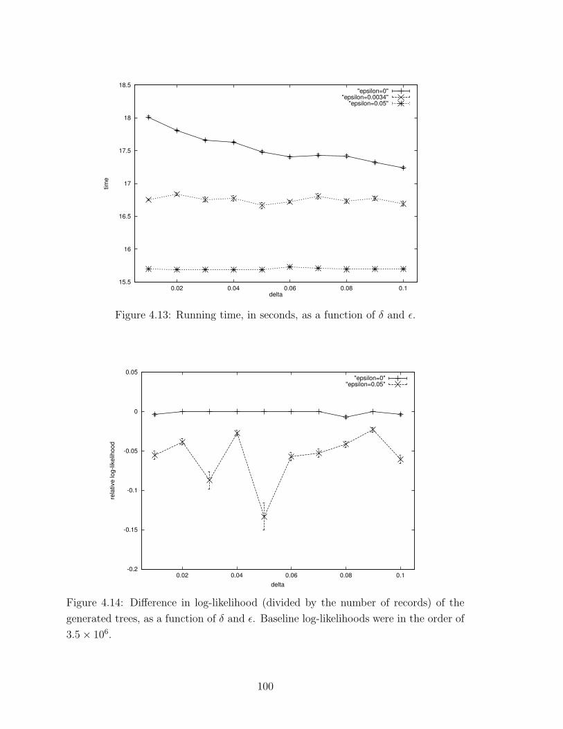
15.5

16

16.5

17

17.5

18

18.5

0.02 0.04 0.06 0.08 0.1

time

delta

"epsilon=0""epsilon=0.0034"

"epsilon=0.05"

Figure 4.13: Running time, in seconds, as a function of δ and ε.

-0.2

-0.15

-0.1

-0.05

0

0.05

0.02 0.04 0.06 0.08 0.1

rela

tive

log-

likel

ihoo

d

delta

"epsilon=0""epsilon=0.05"

Figure 4.14: Difference in log-likelihood (divided by the number of records) of the

generated trees, as a function of δ and ε. Baseline log-likelihoods were in the order of

3.5× 106.

100

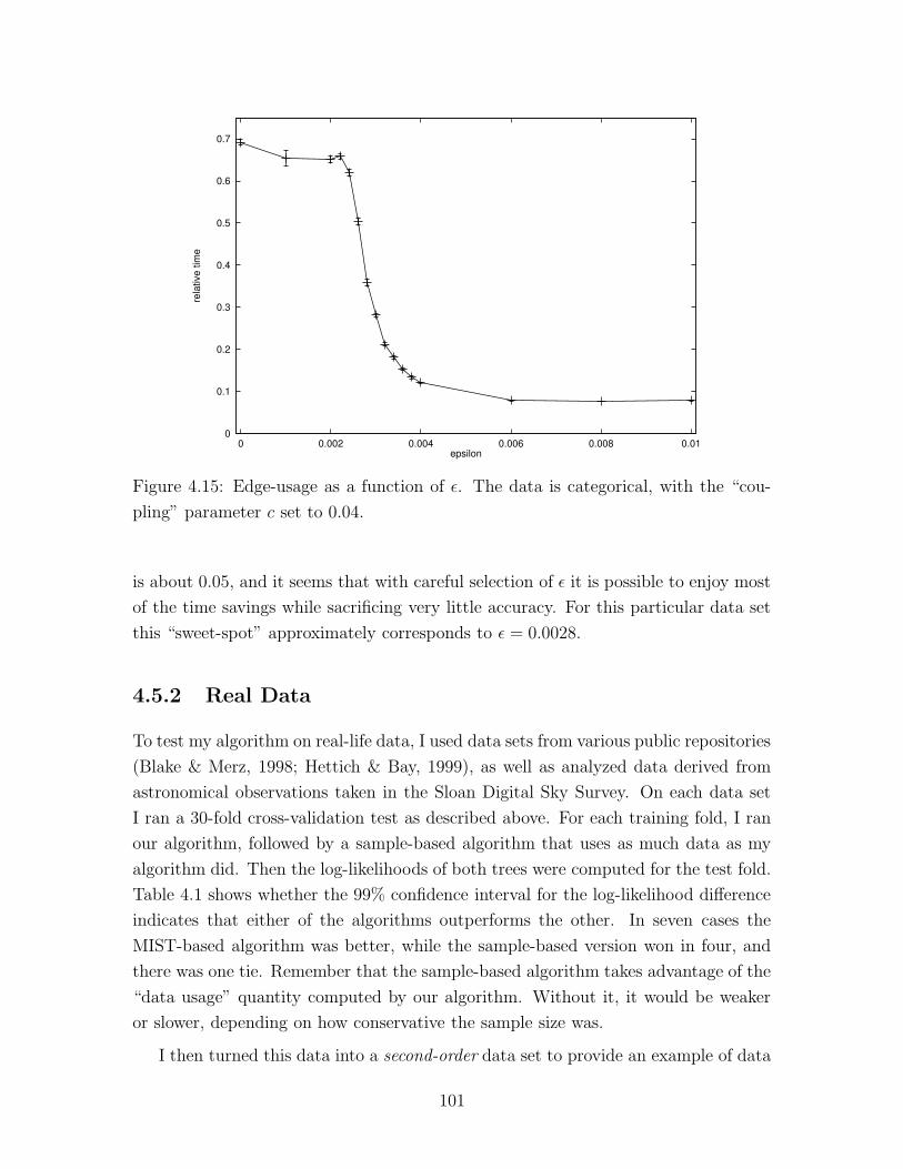
0

0.1

0.2

0.3

0.4

0.5

0.6

0.7

0 0.002 0.004 0.006 0.008 0.01

rela

tive

time

epsilon

Figure 4.15: Edge-usage as a function of ε. The data is categorical, with the “cou-

pling” parameter c set to 0.04.

is about 0.05, and it seems that with careful selection of ε it is possible to enjoy most

of the time savings while sacrificing very little accuracy. For this particular data set

this “sweet-spot” approximately corresponds to ε = 0.0028.

4.5.2 Real Data

To test my algorithm on real-life data, I used data sets from various public repositories

(Blake & Merz, 1998; Hettich & Bay, 1999), as well as analyzed data derived from

astronomical observations taken in the Sloan Digital Sky Survey. On each data set

I ran a 30-fold cross-validation test as described above. For each training fold, I ran

our algorithm, followed by a sample-based algorithm that uses as much data as my

algorithm did. Then the log-likelihoods of both trees were computed for the test fold.

Table 4.1 shows whether the 99% confidence interval for the log-likelihood difference

indicates that either of the algorithms outperforms the other. In seven cases the

MIST-based algorithm was better, while the sample-based version won in four, and

there was one tie. Remember that the sample-based algorithm takes advantage of the

“data usage” quantity computed by our algorithm. Without it, it would be weaker

or slower, depending on how conservative the sample size was.

I then turned this data into a second-order data set to provide an example of data

101

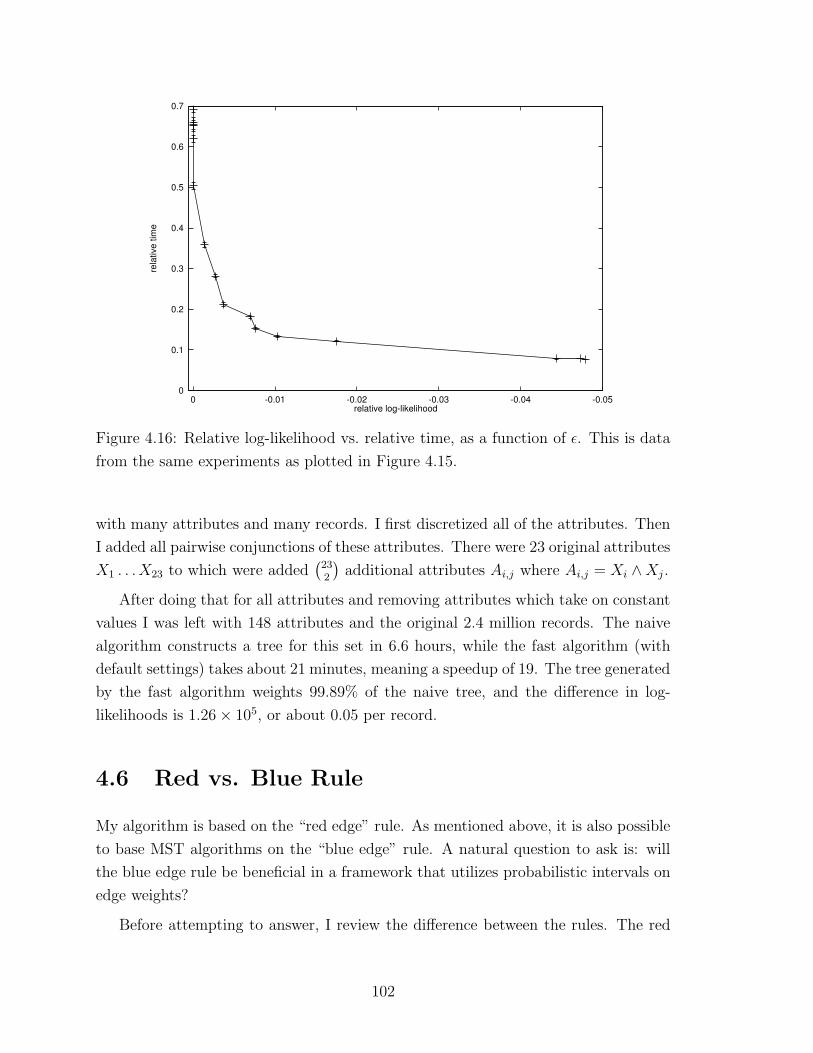
0

0.1

0.2

0.3

0.4

0.5

0.6

0.7

-0.05-0.04-0.03-0.02-0.010

rela

tive

time

relative log-likelihood

Figure 4.16: Relative log-likelihood vs. relative time, as a function of ε. This is data

from the same experiments as plotted in Figure 4.15.

with many attributes and many records. I first discretized all of the attributes. Then

I added all pairwise conjunctions of these attributes. There were 23 original attributes

X1 . . .X23 to which were added(

232

)

additional attributes Ai,j where Ai,j = Xi ∧Xj.

After doing that for all attributes and removing attributes which take on constant

values I was left with 148 attributes and the original 2.4 million records. The naive

algorithm constructs a tree for this set in 6.6 hours, while the fast algorithm (with

default settings) takes about 21 minutes, meaning a speedup of 19. The tree generated

by the fast algorithm weights 99.89% of the naive tree, and the difference in log-

likelihoods is 1.26× 105, or about 0.05 per record.

4.6 Red vs. Blue Rule

My algorithm is based on the “red edge” rule. As mentioned above, it is also possible

to base MST algorithms on the “blue edge” rule. A natural question to ask is: will

the blue edge rule be beneficial in a framework that utilizes probabilistic intervals on

edge weights?

Before attempting to answer, I review the difference between the rules. The red

102

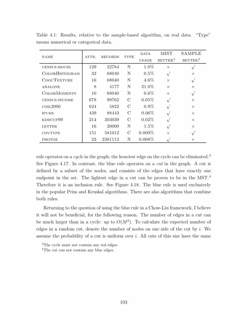
Table 4.1: Results, relative to the sample-based algorithm, on real data. “Type”

means numerical or categorical data.

name attr. records typedata

usage

MIST

better?

SAMPLE

better?

census-house 129 22784 N 1.0% × √

ColorHistogram 32 68040 N 0.5%√ ×

CoocTexture 16 68040 N 4.6% × √

abalone 8 4177 N 21.0% × ×ColorMoments 10 68040 N 0.6% × √

census-income 678 99762 C 0.05%√ ×

coil2000 624 5822 C 0.9%√ ×

ipums 439 88443 C 0.06%√ ×

kddcup99 214 303039 C 0.02%√ ×

letter 16 20000 N 1.5%√ ×

covtype 151 581012 C 0.009% × √

photoz 23 2381112 N 0.008%√ ×

rule operates on a cycle in the graph; the heaviest edge on the cycle can be eliminated.3

See Figure 4.17. In contrast, the blue rule operates on a cut in the graph. A cut is

defined by a subset of the nodes, and consists of the edges that have exactly one

endpoint in the set. The lightest edge in a cut can be proven to be in the MST.4

Therefore it is an inclusion rule. See Figure 4.18. The blue rule is used exclusively

in the popular Prim and Kruskal algorithms. There are also algorithms that combine

both rules.

Returning to the question of using the blue rule in a Chow-Liu framework, I believe

it will not be beneficial, for the following reason. The number of edges in a cut can

be much larger than in a cycle: up to O(M 2). To calculate the expected number of

edges in a random cut, denote the number of nodes on one side of the cut by i. We

assume the probability of a cut is uniform over i. All cuts of this size have the same

3The cycle must not contain any red edges.4The cut can not contain any blue edges.

103

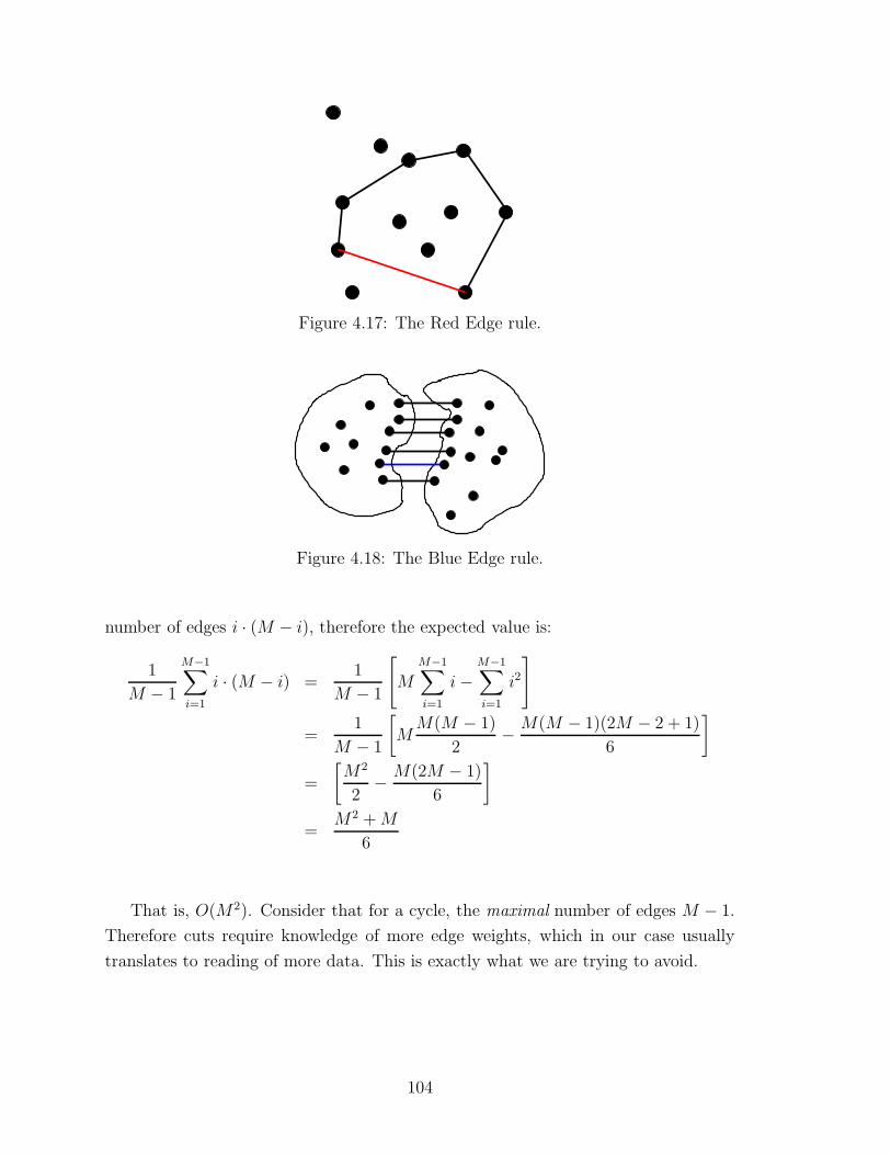
Figure 4.17: The Red Edge rule.

Figure 4.18: The Blue Edge rule.

number of edges i · (M − i), therefore the expected value is:

1

M − 1

M−1∑

i=1

i · (M − i) =1

M − 1

[

MM−1∑

i=1

i−M−1∑

i=1

i2

]

=1

M − 1

[

MM(M − 1)

2− M(M − 1)(2M − 2 + 1)

6

]

=

[

M2

2− M(2M − 1)

6

]

=M2 + M

6

That is, O(M2). Consider that for a cycle, the maximal number of edges M − 1.

Therefore cuts require knowledge of more edge weights, which in our case usually

translates to reading of more data. This is exactly what we are trying to avoid.

104

4.7 Error Analysis

The use of probabilistic bounds means that there is a risk of making a wrong decision.

We now quantify this risk. For the purpose of the analysis, we treat the tree built

by the Chow-Liu algorithm, when given exact edge weights, as optimal. We consider

every deviation from this tree as an error.5 For simplicity we assume that the edge

weights are all unique and so is the optimal weight. We call the edges that form the

optimal tree “optimal edges”. We also ignore the δ optimization (i.e., assume it is set

to zero). The event that we are interested in is that the tree output by the modified

MIST algorithm is identical to the optimal tree.

Consider a MIST run which ends in the optimal tree. It starts with an arbitrary

tree, and eliminates and swaps edges as in Section 4.4. We make two observations.

One, it is sufficient to consider just steps in which an edge is eliminated. This is

true because there is no risk of making a mistake by deferring the decision due to

insufficient data. Two, in all the elimination steps, edges that are not in the optimal

tree are eliminated.

Follow the sequence of execution; each elimination step corresponds to one of the

following scenarios:

1. Eliminate a non-optimal and non-tree edge because it is heavier than a tree

edge.

2. Swap an optimal and a non-optimal edge because the optimal edge is lighter.

The non-optimal edge swapped out from the current tree is then eliminated.

In both cases, a non-optimal edge is eliminated because a weight comparison de-

termines it is heavier than an optimal edge. We calculate the probability of arriving

at the opposite decision erroneously. Let A be the true weight of the optimal edge

(meaning the value used by the original Chow-Liu algorithm), and let a be the corre-

sponding confidence interval. Similarly, let B be the true value for the non-optimal

edge and b its interval. See Figure 4.19.

In our case B > A. A mistake happens by having a and b such that the edge

associated with a is eliminated. Since the algorithm defers all decisions based on

overlapping intervals, the only configuration allowing this is where min(a) > max(b)

(see Figure 4.19(d)). Given that B > A, this cannot hold if both a and b contain their

5A less strict error analysis would consider the expected weight difference between the generated

and optimal trees. Conceivably one could make some assumptions on edge weight distribution to

perform this kind of analysis.

105

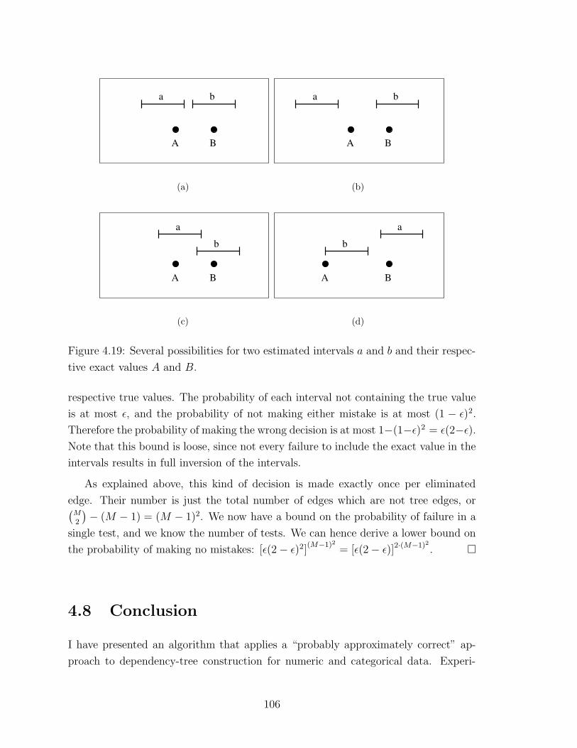
A B

a b

(a)

A B

a b

(b)

A B

a

b

(c)

a

BA

b

(d)

Figure 4.19: Several possibilities for two estimated intervals a and b and their respec-

tive exact values A and B.

respective true values. The probability of each interval not containing the true value

is at most ε, and the probability of not making either mistake is at most (1 − ε)2.

Therefore the probability of making the wrong decision is at most 1−(1−ε)2 = ε(2−ε).

Note that this bound is loose, since not every failure to include the exact value in the

intervals results in full inversion of the intervals.

As explained above, this kind of decision is made exactly once per eliminated

edge. Their number is just the total number of edges which are not tree edges, or(

M2

)

− (M − 1) = (M − 1)2. We now have a bound on the probability of failure in a

single test, and we know the number of tests. We can hence derive a lower bound on

the probability of making no mistakes: [ε(2− ε)2](M−1)2

= [ε(2− ε)]2·(M−1)2 . �

4.8 Conclusion

I have presented an algorithm that applies a “probably approximately correct” ap-

proach to dependency-tree construction for numeric and categorical data. Experi-

106

ments in sets with up to millions of records and hundreds of attributes show it is

capable of processing massive data sets in time that is constant in the number of

records, with just a minor loss in output quality.

Future work includes embedding my algorithm in a framework for fast Bayes Net

structure search.

A additional issue I would like to tackle is disk access. One advantage the full-data

algorithm has is that it is easily executed with a single sequential scan of the data

file. I will explore the ways in which this behavior can be attained or approximated

by my algorithm.

While I derived formulas for both numeric and categorical data, I currently do

not allow both types of attributes to be present in a single network.

107

Chapter 5

Active Learning for Anomaly

Detection

Consider an astronomer who needs to sift through a large set of sky survey images,

each of which comes with many real-valued parameters. Most of the objects (say

99.9%) are well explained by current theories and models. For the remainder of this

chapter we consider them not interesting, since our goal is to find the extraordinary

objects which are worthy of further research. For example, the astronomer might

want to cross-check such objects in various databases and allocate telescope time to

observe them in greater detail.

The remaining data are anomalies, but 99% of these anomalies are uninteresting.

These are records which are strange for mundane reasons such as sensor faults or

problems in the image processing software. Only 1% of the remainder (0.001% of the

full data set) are useful. The goal of my work in this chapter is finding this set of

rare and useful anomalies.

5.1 Introduction

The following example concerns astrophysics, but the same scenario can arise wherever

there is a very large amount of scientific, medical, business or intelligence data. In this

example, a domain expert wants to find truly exotic rare events while not becoming

swamped with uninteresting anomalies.

The “rare events” are distinguished from the traditional statistical definition of

anomalies as outliers or merely ill-modeled points. My distinction is that the useful-

109

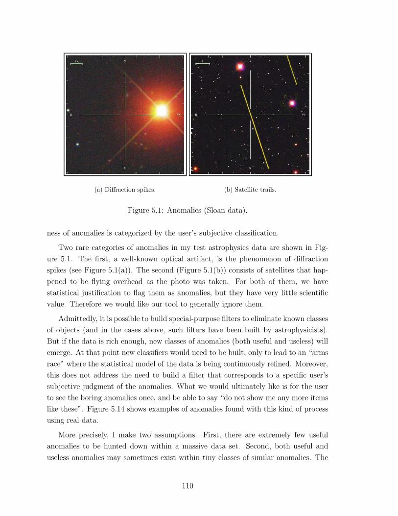
(a) Diffraction spikes. (b) Satellite trails.

Figure 5.1: Anomalies (Sloan data).

ness of anomalies is categorized by the user’s subjective classification.

Two rare categories of anomalies in my test astrophysics data are shown in Fig-

ure 5.1. The first, a well-known optical artifact, is the phenomenon of diffraction

spikes (see Figure 5.1(a)). The second (Figure 5.1(b)) consists of satellites that hap-

pened to be flying overhead as the photo was taken. For both of them, we have

statistical justification to flag them as anomalies, but they have very little scientific

value. Therefore we would like our tool to generally ignore them.

Admittedly, it is possible to build special-purpose filters to eliminate known classes

of objects (and in the cases above, such filters have been built by astrophysicists).

But if the data is rich enough, new classes of anomalies (both useful and useless) will

emerge. At that point new classifiers would need to be built, only to lead to an “arms

race” where the statistical model of the data is being continuously refined. Moreover,

this does not address the need to build a filter that corresponds to a specific user’s

subjective judgment of the anomalies. What we would ultimately like is for the user

to see the boring anomalies once, and be able to say “do not show me any more items

like these”. Figure 5.14 shows examples of anomalies found with this kind of process

using real data.

More precisely, I make two assumptions. First, there are extremely few useful

anomalies to be hunted down within a massive data set. Second, both useful and

useless anomalies may sometimes exist within tiny classes of similar anomalies. The

110

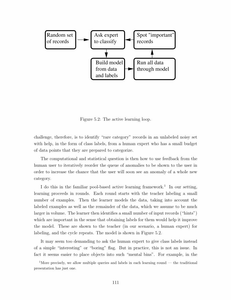
of records Random set Ask expert

to classify

Build modelfrom dataand labels

Run all datathrough model

Spot "important"records

Figure 5.2: The active learning loop.

challenge, therefore, is to identify “rare category” records in an unlabeled noisy set

with help, in the form of class labels, from a human expert who has a small budget

of data points that they are prepared to categorize.

The computational and statistical question is then how to use feedback from the

human user to iteratively reorder the queue of anomalies to be shown to the user in

order to increase the chance that the user will soon see an anomaly of a whole new

category.

I do this in the familiar pool-based active learning framework.1 In our setting,

learning proceeds in rounds. Each round starts with the teacher labeling a small

number of examples. Then the learner models the data, taking into account the

labeled examples as well as the remainder of the data, which we assume to be much

larger in volume. The learner then identifies a small number of input records (“hints”)

which are important in the sense that obtaining labels for them would help it improve

the model. These are shown to the teacher (in our scenario, a human expert) for

labeling, and the cycle repeats. The model is shown in Figure 5.2.

It may seem too demanding to ask the human expert to give class labels instead

of a simple “interesting” or “boring” flag. But in practice, this is not an issue. In

fact it seems easier to place objects into such “mental bins”. For example, in the

1More precisely, we allow multiple queries and labels in each learning round — the traditional

presentation has just one.

111

astronomical data we have seen a user place most objects into previously-known

categories: point sources, low-surface-brightness galaxies, etc. This also holds for the

negative examples: it is frustrating to have to label all anomalies as “bad” without

being able to explain why. In fact, the data is better understood as time goes by, and

people like to revise some of their old labels in light of new examples. Remember that

the statistical model does not care about the names of the labels. For all it cares, the

label set can change completely from one round to another. My tools allow exactly

that: the labels are unconstrained and the user can add, refine, and delete classes

at will. Certainly it is possible to accommodate the simplistic “interesting or not”

model in this richer framework.

My work differs from traditional applications of active learning in that I assume

the distribution of class sizes to be extremely skewed. Typically, the smallest class

may have just a few members whereas the largest may contain a few million. Generally

in active learning, it is believed that, right from the start, examples from each class

need to be presented to the oracle (Basu et al., 2004; Seeger, 2000; Brinker, 2003). If

the class frequencies were balanced, this could be achieved by random sampling. But

in data sets with the rare categories property, this no longer holds, and much of my

effort is an attempt to remedy the situation.2

Previous active-learning work tends to tie intimately to a particular model (Cohn

et al., 1995; Brinker, 2003). In contrast, I would like to be able to “plug in” different

types of models or components and therefore propose model-independent criteria.

The same reasoning also precludes us from directly using distances between data

points, as is done in Wiratunga et al. (2003). The only assumption I make is that

my model is a mixture, and each component is a probability density estimator.

Another desired property is resilience to noise. Noise can be inherent in the data

(e.g., from measurement errors) or be an artifact of a ill-fitting model. In any case,

we need to be able to identify query points in the presence of noise. This is a not just

a bonus feature: points which the model considers noisy could very well be the key

to improvement if presented to the oracle. This is in contrast to the approach taken

by Cohn et al. (1994) and Plutowski and White (1993): a pre-assumption that the

data is noiseless.

2However, it is interesting to note that in some cases, it is useful to add a random sampling

expert to an ensemble (Baram et al., 2003).

112

Figure 5.3: Underlying data distribution for the example.

5.2 Overview of Hint Selection Methods

In this section we survey several proposed methods for active learning as they apply

to our setting. We give anecdotal evidence of their weaknesses. While the general

tone is negative, what follows should not be construed as general dismissal of these

methods. Rather, it is meant to highlight specific problems with them when applied

to a particular setting.

The data shown (Figure 5.3) is a mixture of two classes. One is an X-shaped dis-

tribution, from which 2000 points are drawn. The other is a circle with 100 points. In

this example, the classifier is a Gaussian Bayes classifier trained in a semi-supervised

manner from labeled and unlabeled data, with one Gaussian per class. The model

is learned with a standard EM procedure, with the following straightforward mod-

ification (Shahshashani & Landgrebe, 1994; Miller & Uyar, 1997) to enable semi-

supervised learning. Before each M step we clamp the class membership values for

the hinted records to match the hints (i.e., one for the labeled class for this record,

and zero elsewhere).

Given fully labeled data, our learner would perfectly predict class membership for

this data3: one Gaussian centered on the circle, and another spherical Gaussian with

high variance centered on the X. Now, suppose we plan to perform active learning in

which we take the following steps:

1. Start with entirely unlabeled data.

2. Perform semi-supervised learning (which, on the first iteration degenerates to

3It would, however, be a poor generative model.

113

unsupervised learning).

3. Ask an expert to classify the 35 strangest records.

4. Go to Step 2.

On the first iteration (when unsupervised) the algorithm will naturally use the two

Gaussians to model the data as in Figure 5.4(b), with one Gaussian for each of the

arms of the “X”, and the points in the circle represented as members of one of them.

What happens next all depends on the choice of the data points to show to the human

expert.

We now survey the previously published methods for hint selection.

5.2.1 Choosing Points with Low Likelihood

A rather intuitive approach is to select as hints the points which the model performs

worst on. This can be viewed as model variance minimization (as in Cohn et al.

(1995)) or as selection of points furthest away from any labeled points (Wiratunga

et al., 2003). We do this by ranking each point in order of increasing model likelihood,

and choosing the top items.

I show what this approach would flag in the given configuration in Figure 5.4. It

is derived from a screenshot of a running version of my code, and is hand-drawn for

clarity. Each subsequent drawing shows a model which EM converged to in one round,

and the hints it chooses under a particular scheme (here it is what we call lowlik).

These hints affect the model shown for the next round. The underlying distribution

is shown in gray shading. We use this convention for the other methods below.

In the first round, the Mahalanobis distance for the points in the corners is greater

than those in the circle, therefore they are flagged. Another effect we see is that one

of the arms is over-represented. This is probably due to its lower variance. In any

event, none of the points in the circle is flagged. The outcome is that the next round

ends up in a similar local minimum. We can also see that another step will not result

in the desired model. Only after obtaining labels for all of the “outlier” points (that

is, those on the extremes of the distribution) will this approach go far enough down

the list to hit a point in the circle. This means that in scenarios where there are more

than a few hundred noisy data, classification accuracy is likely to be very low.

114

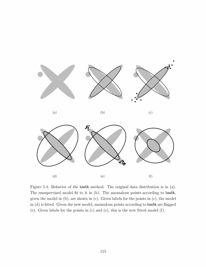
(a) (b) (c)

(d) (e) (f)

Figure 5.4: Behavior of the lowlik method. The original data distribution is in (a).

The unsupervised model fit to it in (b). The anomalous points according to lowlik,

given the model in (b), are shown in (c). Given labels for the points in (c), the model

in (d) is fitted. Given the new model, anomalous points according to lowlik are flagged

(e). Given labels for the points in (c) and (e), this is the new fitted model (f).

115

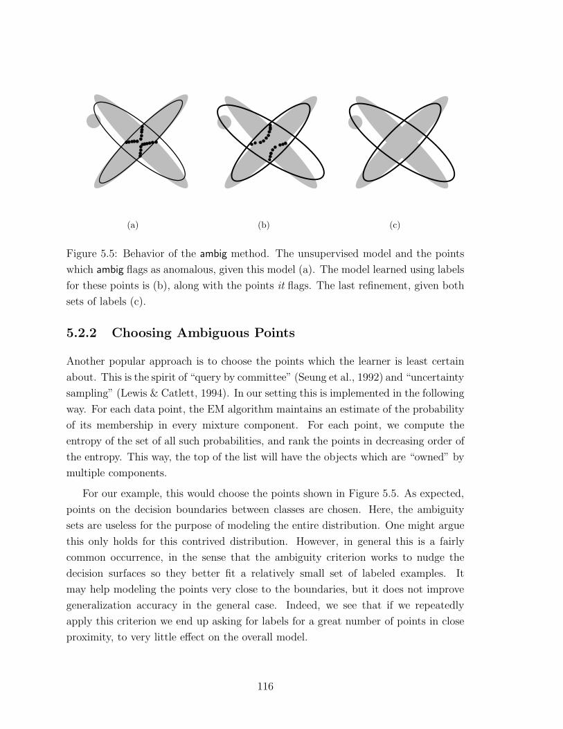
(a) (b) (c)

Figure 5.5: Behavior of the ambig method. The unsupervised model and the points

which ambig flags as anomalous, given this model (a). The model learned using labels

for these points is (b), along with the points it flags. The last refinement, given both

sets of labels (c).

5.2.2 Choosing Ambiguous Points

Another popular approach is to choose the points which the learner is least certain

about. This is the spirit of “query by committee” (Seung et al., 1992) and “uncertainty

sampling” (Lewis & Catlett, 1994). In our setting this is implemented in the following

way. For each data point, the EM algorithm maintains an estimate of the probability

of its membership in every mixture component. For each point, we compute the

entropy of the set of all such probabilities, and rank the points in decreasing order of

the entropy. This way, the top of the list will have the objects which are “owned” by

multiple components.

For our example, this would choose the points shown in Figure 5.5. As expected,

points on the decision boundaries between classes are chosen. Here, the ambiguity

sets are useless for the purpose of modeling the entire distribution. One might argue

this only holds for this contrived distribution. However, in general this is a fairly

common occurrence, in the sense that the ambiguity criterion works to nudge the

decision surfaces so they better fit a relatively small set of labeled examples. It

may help modeling the points very close to the boundaries, but it does not improve

generalization accuracy in the general case. Indeed, we see that if we repeatedly

apply this criterion we end up asking for labels for a great number of points in close

proximity, to very little effect on the overall model.

116

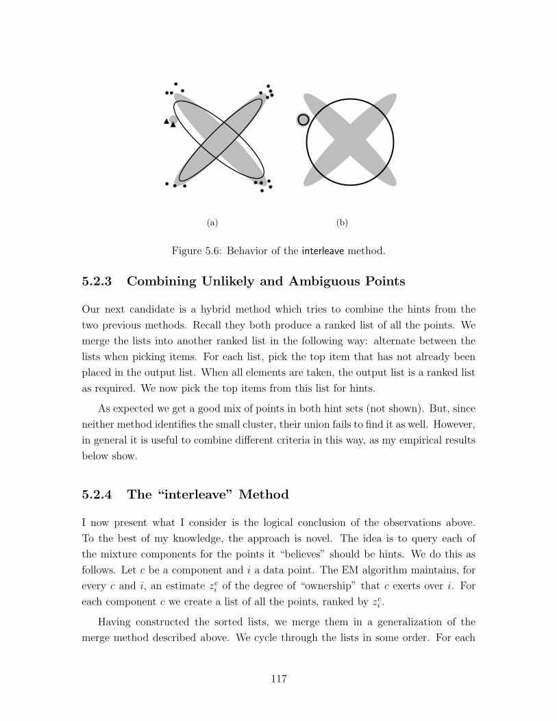
(a) (b)

Figure 5.6: Behavior of the interleave method.

5.2.3 Combining Unlikely and Ambiguous Points

Our next candidate is a hybrid method which tries to combine the hints from the

two previous methods. Recall they both produce a ranked list of all the points. We

merge the lists into another ranked list in the following way: alternate between the

lists when picking items. For each list, pick the top item that has not already been

placed in the output list. When all elements are taken, the output list is a ranked list

as required. We now pick the top items from this list for hints.

As expected we get a good mix of points in both hint sets (not shown). But, since

neither method identifies the small cluster, their union fails to find it as well. However,

in general it is useful to combine different criteria in this way, as my empirical results

below show.

5.2.4 The “interleave” Method

I now present what I consider is the logical conclusion of the observations above.

To the best of my knowledge, the approach is novel. The idea is to query each of

the mixture components for the points it “believes” should be hints. We do this as

follows. Let c be a component and i a data point. The EM algorithm maintains, for

every c and i, an estimate zci of the degree of “ownership” that c exerts over i. For

each component c we create a list of all the points, ranked by zci .

Having constructed the sorted lists, we merge them in a generalization of the

merge method described above. We cycle through the lists in some order. For each

117

list, we pick the top item that has not already been placed in the output list, and

place it at the next position in the output list.

The results for this strategy are shown in Figure 5.6. We see it meets the require-

ment of comprehensive representation for all true components. Most of the points

are along the major axes of the two elongated Gaussians, but two of the points are

inside the small circle. Correct labels for even just these two points result in perfect

classification in the next EM run.

To gain insight for this method we look at the estimates zci . These are measures

of the conditional likelihood of point i given that it was generated by component c,

normalized by the sum of the same measure over all components c′. To minimize

zci the point needs to have a low conditional likelihood for c (this is the numerator)

and a high denominator. For a high sum over all components, it is not enough for

a point to be nearly uniquely owned by a single component. Rather, it needs to be

fairly equally “divided” among the components. Intuitively, this means that for a

component c to nominate a point, it needs to be considered unlikely for c, and also

not obviously belong to some other component. This means that each component c

identifies low-likelihood points that are “orphaned” by all of the other components.

Using separate component lists, we can in fact detect two different kinds of mis-

modeled points. See Figure 5.7. The first kind are points which are associated

with some component, and are similar in many ways to most of the other points in

it. However they are slightly different — for example, they may have an outlying

value in just one attribute. These points will be flagged because they are in a low-

density region for this components. The other kind are points which are isolated in

“empty” regions, and do not naturally belong to a particular component. In some

cases these points will be picked up by the closest (in density space) component, and

will be flagged in the same way. But it is also possible to introduce a uniform-density

“background” component. This component gets to nominate in the usual way. By its

nature, it picks up the “orphan” points which do not naturally belong to any other

component. This way, isolated points will be ranked highly in the hint list.

Admittedly, the discussion above is merely an illustrative example. Below I present

empirical evidence further supporting the same ideas.

118

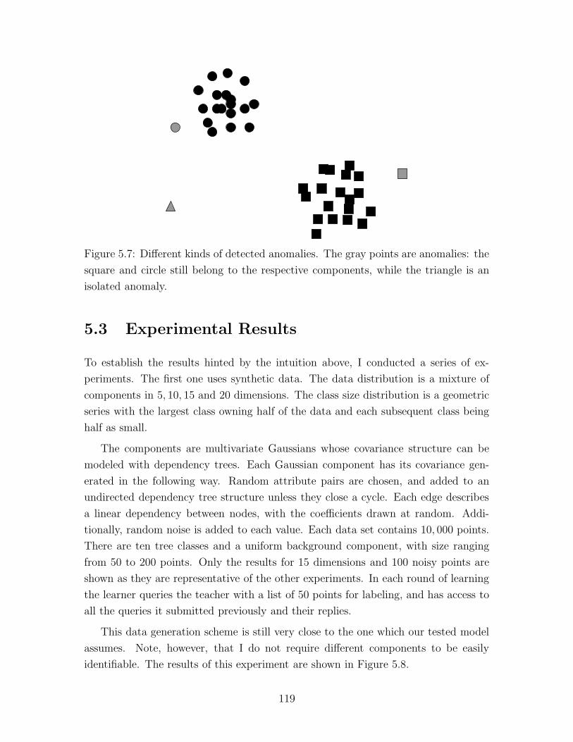
Figure 5.7: Different kinds of detected anomalies. The gray points are anomalies: the

square and circle still belong to the respective components, while the triangle is an

isolated anomaly.


To establish the results hinted by the intuition above, I conducted a series of ex-

periments. The first one uses synthetic data. The data distribution is a mixture of

components in 5, 10, 15 and 20 dimensions. The class size distribution is a geometric

series with the largest class owning half of the data and each subsequent class being

half as small.

The components are multivariate Gaussians whose covariance structure can be

modeled with dependency trees. Each Gaussian component has its covariance gen-

erated in the following way. Random attribute pairs are chosen, and added to an

undirected dependency tree structure unless they close a cycle. Each edge describes

a linear dependency between nodes, with the coefficients drawn at random. Addi-

tionally, random noise is added to each value. Each data set contains 10, 000 points.

There are ten tree classes and a uniform background component, with size ranging

from 50 to 200 points. Only the results for 15 dimensions and 100 noisy points are

shown as they are representative of the other experiments. In each round of learning

the learner queries the teacher with a list of 50 points for labeling, and has access to

all the queries it submitted previously and their replies.

This data generation scheme is still very close to the one which our tested model

assumes. Note, however, that I do not require different components to be easily

identifiable. The results of this experiment are shown in Figure 5.8.

119

Our scoring function is driven by our application, and estimates the amount of

effort the teacher has to expend before being presented by representatives of every

single class. The assumption is that the teacher can generalize from a single example

(or a very few examples) to an entire class, and the valuable information is concen-

trated in the first queried member of each class. More precisely, if there are n classes,

then the score under this metric is 1/n times the number of classes represented in the

query set. In the query set I include all items queried in preceding rounds, as I do for

other applicable metrics.

We now list of the names of the algorithms as they appear in the graphs, and a

short description for each.

• lowlik This algorithm lists the least likely points first as described in Sec-

tion 5.2.1.

• ambig This algorithm lists the most ambiguous points first as described in Sec-

tion 5.2.2.

• mix-ambig-lowlik This algorithm merges the lists of lowlik and abmig as described

in Section 5.2.3.

• interleave This algorithm lets each component “nominate” hints as described in

Section 5.2.4, with the following modification. The background uniform-density

component gets to nominate more often than any other component. In terms of

list merging, we take one element from each of the lists of standard components,

and then several elements from the list produced for the background component.

All of the results shown were obtained using an oversampling ratio of 20.

• random This is a baseline method which chooses hints at random.

The best performer so far is interleave, taking five rounds or less to reveal all of the

classes, including the very rare ones. Below I show how it is superior in most of the

real-life data sets as well. We can also see that ambig performs worse than random.

This can be explained by the fact that ambig only chooses points that already have

several existing components “competing” for them. Rarely do these points belong to

a new, yet-undiscovered component.

I was concerned that the poor performance of lowlik was just a consequence of my

choice of metric. After all, it does not measure the number of noise points found.

So it is possible that lowlik is being penalized unfairly for its focusing on the noise

points. After examining the fraction of noise points (i.e., points drawn from the

120

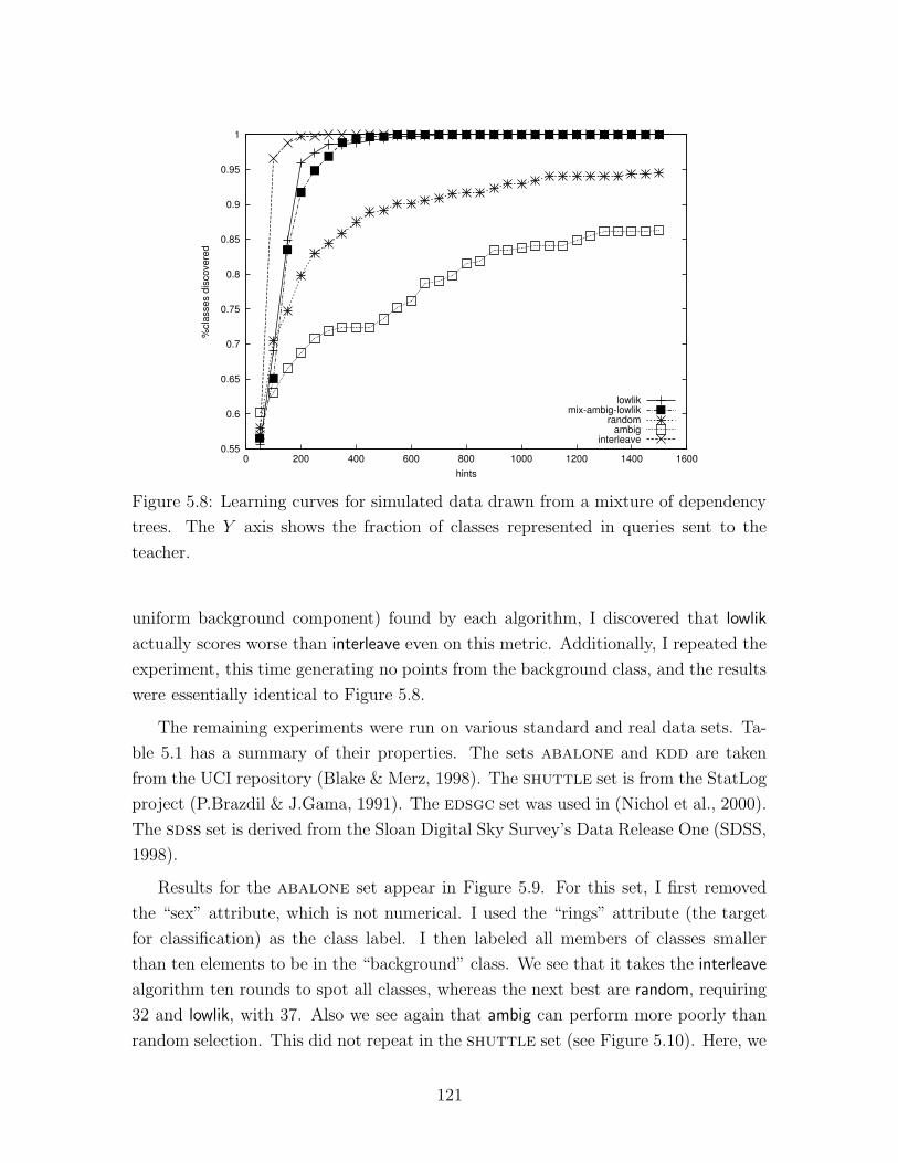
0.55

0.6

0.65

0.7

0.75

0.8

0.85

0.9

0.95

1

0 200 400 600 800 1000 1200 1400 1600

%cl

asse

s di

scov

ered

hints

lowlikmix-ambig-lowlik

randomambig

interleave

Figure 5.8: Learning curves for simulated data drawn from a mixture of dependency

trees. The Y axis shows the fraction of classes represented in queries sent to the

teacher.

uniform background component) found by each algorithm, I discovered that lowlik

actually scores worse than interleave even on this metric. Additionally, I repeated the

experiment, this time generating no points from the background class, and the results

were essentially identical to Figure 5.8.

The remaining experiments were run on various standard and real data sets. Ta-

ble 5.1 has a summary of their properties. The sets abalone and kdd are taken

from the UCI repository (Blake & Merz, 1998). The shuttle set is from the StatLog

project (P.Brazdil & J.Gama, 1991). The edsgc set was used in (Nichol et al., 2000).

The sdss set is derived from the Sloan Digital Sky Survey’s Data Release One (SDSS,

1998).

Results for the abalone set appear in Figure 5.9. For this set, I first removed

the “sex” attribute, which is not numerical. I used the “rings” attribute (the target

for classification) as the class label. I then labeled all members of classes smaller

than ten elements to be in the “background” class. We see that it takes the interleave

algorithm ten rounds to spot all classes, whereas the next best are random, requiring

32 and lowlik, with 37. Also we see again that ambig can perform more poorly than

random selection. This did not repeat in the shuttle set (see Figure 5.10). Here, we

121

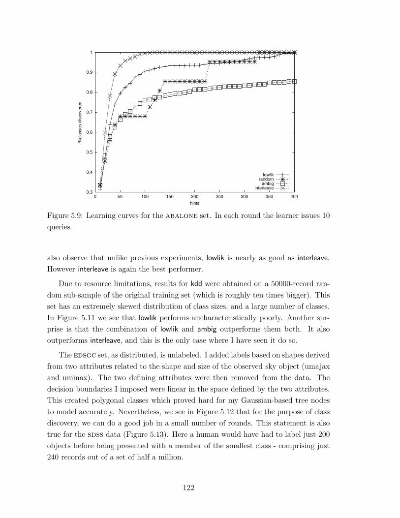
0.3

0.4

0.5

0.6

0.7

0.8

0.9

1

0 50 100 150 200 250 300 350 400

%cl

asse

s di

scov

ered

hints

lowlikrandom

ambiginterleave

Figure 5.9: Learning curves for the abalone set. In each round the learner issues 10

queries.

also observe that unlike previous experiments, lowlik is nearly as good as interleave.

However interleave is again the best performer.

Due to resource limitations, results for kdd were obtained on a 50000-record ran-

dom sub-sample of the original training set (which is roughly ten times bigger). This

set has an extremely skewed distribution of class sizes, and a large number of classes.

In Figure 5.11 we see that lowlik performs uncharacteristically poorly. Another sur-

prise is that the combination of lowlik and ambig outperforms them both. It also

outperforms interleave, and this is the only case where I have seen it do so.

The edsgc set, as distributed, is unlabeled. I added labels based on shapes derived

from two attributes related to the shape and size of the observed sky object (umajax

and uminax). The two defining attributes were then removed from the data. The

decision boundaries I imposed were linear in the space defined by the two attributes.

This created polygonal classes which proved hard for my Gaussian-based tree nodes

to model accurately. Nevertheless, we see in Figure 5.12 that for the purpose of class

discovery, we can do a good job in a small number of rounds. This statement is also

true for the sdss data (Figure 5.13). Here a human would have had to label just 200

objects before being presented with a member of the smallest class - comprising just

240 records out of a set of half a million.

122

0.4

0.5

0.6

0.7

0.8

0.9

1

0 500 1000 1500 2000 2500 3000

%cl

asse

s di

scov

ered

hints

lowlikrandom

ambiginterleave

Figure 5.10: Learning curves for the shuttle set. In each round the learner issues

100 queries.

0.1

0.2

0.3

0.4

0.5

0.6

0.7

0.8

0.9

0 50 100 150 200 250 300 350 400

%cl

asse

s di

scov

ered

hints

lowlikmix-ambig-lowlik

randomambig

interleave

Figure 5.11: Learning curves for the kdd set. In each round the learner issues 20

queries.

123

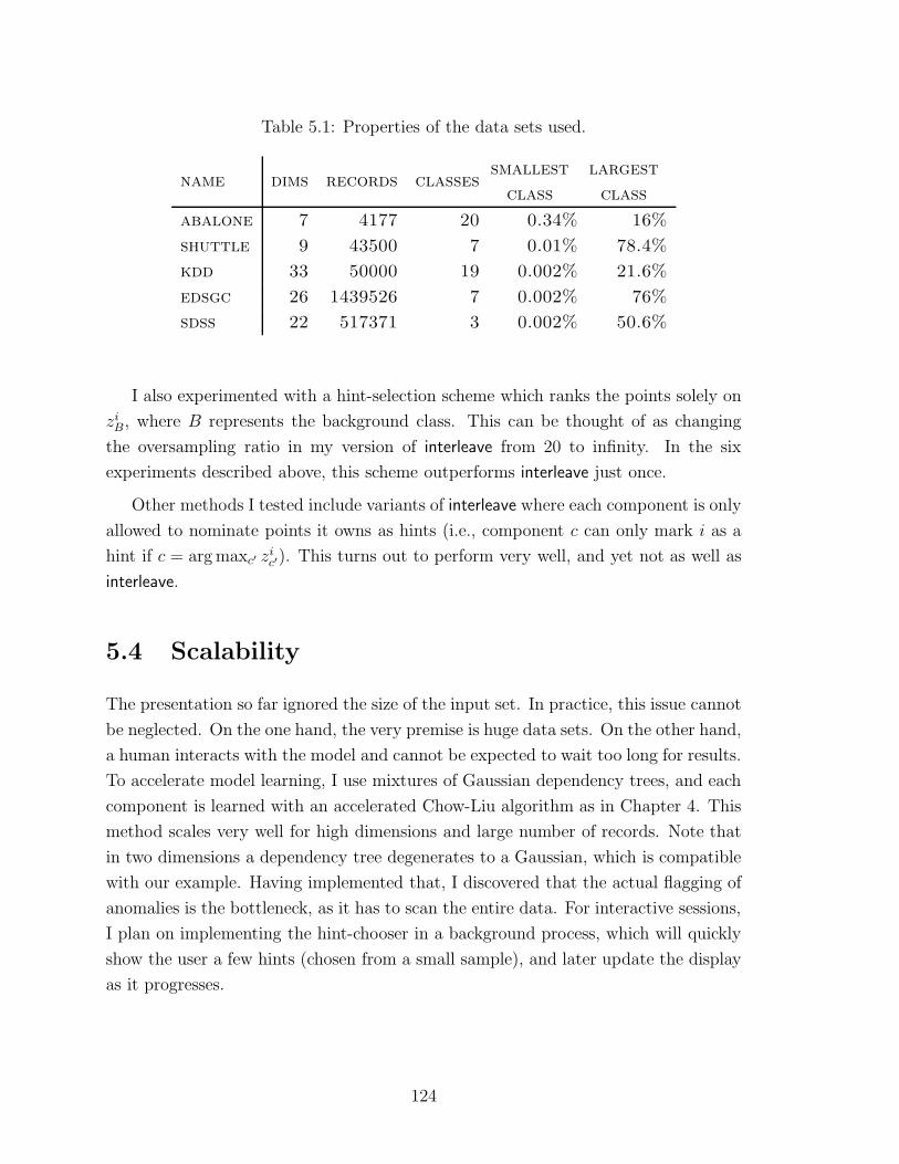
Table 5.1: Properties of the data sets used.

name dims records classessmallest

class

largest

class

abalone 7 4177 20 0.34% 16%

shuttle 9 43500 7 0.01% 78.4%

kdd 33 50000 19 0.002% 21.6%

edsgc 26 1439526 7 0.002% 76%

sdss 22 517371 3 0.002% 50.6%

I also experimented with a hint-selection scheme which ranks the points solely on

ziB, where B represents the background class. This can be thought of as changing

the oversampling ratio in my version of interleave from 20 to infinity. In the six

experiments described above, this scheme outperforms interleave just once.

Other methods I tested include variants of interleave where each component is only

allowed to nominate points it owns as hints (i.e., component c can only mark i as a

hint if c = arg maxc′ zic′). This turns out to perform very well, and yet not as well as

interleave.

5.4 Scalability

The presentation so far ignored the size of the input set. In practice, this issue cannot

be neglected. On the one hand, the very premise is huge data sets. On the other hand,

a human interacts with the model and cannot be expected to wait too long for results.

To accelerate model learning, I use mixtures of Gaussian dependency trees, and each

component is learned with an accelerated Chow-Liu algorithm as in Chapter 4. This

method scales very well for high dimensions and large number of records. Note that

in two dimensions a dependency tree degenerates to a Gaussian, which is compatible

with our example. Having implemented that, I discovered that the actual flagging of

anomalies is the bottleneck, as it has to scan the entire data. For interactive sessions,

I plan on implementing the hint-chooser in a background process, which will quickly

show the user a few hints (chosen from a small sample), and later update the display

as it progresses.

124

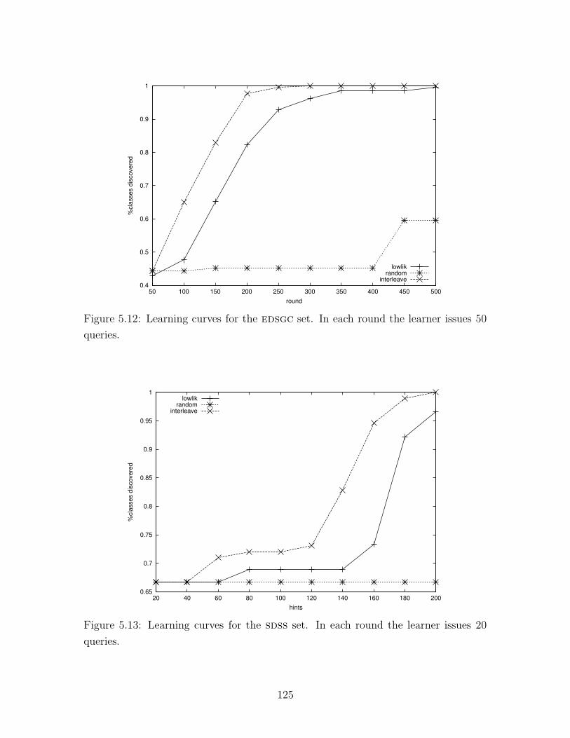
0.4

0.5

0.6

0.7

0.8

0.9

1

50 100 150 200 250 300 350 400 450 500

%cl

asse

s di

scov

ered

round

lowlikrandom

interleave

Figure 5.12: Learning curves for the edsgc set. In each round the learner issues 50

queries.

0.65

0.7

0.75

0.8

0.85

0.9

0.95

1

20 40 60 80 100 120 140 160 180 200

%cl

asse

s di

scov

ered

hints

lowlikrandom

interleave

Figure 5.13: Learning curves for the sdss set. In each round the learner issues 20

queries.

125

5.5 Conclusion

I have shown that some of the popular methods for active learning perform poorly

in realistic active-learning scenarios. Working from the definition of a mixture model

I was able to propose methods which let each component “nominate” its favorite

queries. These methods work well in the presence of noisy data and extremely rare

classes and anomalies. My simulations show that a human user only needs to label

one or two hundred examples before being presented with very rare anomalies in huge

data sets. This kind of interaction typically takes just an hour or two of combined

human and computer time.

Furthermore, I make no assumptions about the particular form a component takes

(beside it being a PDE). Consequently, I expect my results to apply to many different

kinds of component models, including the case where components are not all from

the same distribution.

I am using lessons learned from my empirical comparison in an application for

anomaly-hunting in the astrophysics domain. My application presents multiple in-

dicators to help a user spot anomalous data, as well as controls for labeling points

and adding classes. Some interesting objects found after a few rounds of interaction

with the Sloan data are shown in Figure 5.14. The application will be described in

Chapter 6.

126

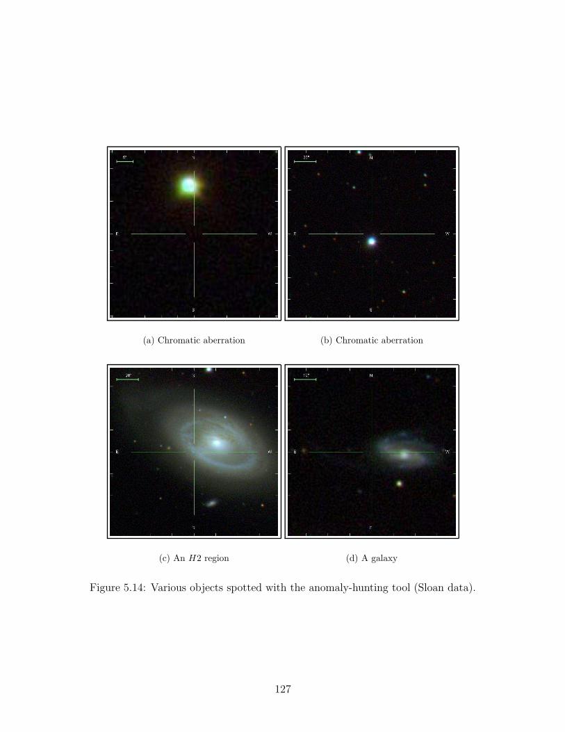
(a) Chromatic aberration (b) Chromatic aberration

(c) An H2 region (d) A galaxy

Figure 5.14: Various objects spotted with the anomaly-hunting tool (Sloan data).

127

Chapter 6

Anomaly Hunting

This chapter describes a data-mining application which builds on the methods out-

lined in Chapter 5. The task is anomaly hunting in large data sets. The tool is

generally geared towards astronomical observations, but can be directly applied to

other kinds of data. I outline a new process using a combination of a graphical appli-

cation, and the algorithmic techniques from the previous chapters. I also conducted

a case study with a cosmologist analyzing SDSS data, and report the results.

6.1 Background

Before I start describing the new anomaly hunting process, I outline how similar

analyses were carried out at the early stages of my involvement with such work.

First, the raw data was not as well-organized as it is now. Mappings from object

identifiers to image cutouts had to be done by hand. Once the images were obtained,

they were viewed with generic image viewing and manipulation tools. Consequently,

any kind of feedback had to also be carried over manually.

The main feedback loop proceeded as follows. After a night of telescope obser-

vations the results would be informally analyzed. Common characteristics of the

anomalous objects which were boring or produced bad results were defined. Then, a

predicate to filter them out of the data set was written manually. The cleaned data

was fed to a learner and was fitted by a mixture of dependency trees. This is the

same model as currently used. However no individual labels were assigned because

of the difficulty of doing so. Instead, the learner itself decided how to split the data

among classes. The current learner still has this capability, but it falls back to it only

in the absence of specific labels.

129

Figure 6.1: The anomaly hunting application.

6.2 Indicators and Controls

The main interaction screen for the current tool is shown in Figure 6.1. On the left we

see “postage stamp” photos of several objects. The objects are shown as ordered by

the anomaly hunting algorithm. Generally speaking, the least well-explained object

is in the top spot, and the objects are “more normal” as one progresses down the list.

The user can scroll the list of objects to see other batches of photos.

The colored rectangles on the right indicate the value each object takes on for

different attributes. The goal is to provide a quick way of comparing numerical values.

Each column of rectangles is for a different attribute. For example, all the leftmost

rectangles in the picture stand for the value of “isoAGrad r” for the respective objects.

The values are quantized and color-coded. Black means the value for this object and

attribute is close to the median for the attribute, taken over the entire data. Red

means above median, and the brighter shade of red is used, the higher quantile the

value falls in. Similarly, green means under-median values, with the darkest green

standing for the lowest value.

130

Figure 6.2: The object information window.

The class buttons (labeled c0 through c6 in this example) let the user assign labels

to objects. Whenever the user believes that an object naturally belongs to a certain

class, he or she can check the box next to the appropriate label. The names are

arbitrary and selected by the user. Multiple labels are supported, as well as assigning

no label. New labels can be created freely.

The “locked” button indicates that the underlying statistical modeling stage may

not re-assign this object to a class other than the one specified by the user. By default

it is selected. If it is not, the specified label is used to seed the EM process, but can

otherwise change if this (locally) improves the fit.

The “zoom” controls let the user zoom the photo in and out. This is supported by

an on-line repository which provides arbitrary image cut-outs. The SkyServer (Szalay

et al., 2004) is one such repository which we use for the astronomical data.

When selecting an object, a window with detailed information about the object

pops up. An example is shown in Figure 6.2. It simply lists the exact values for the

object in each of a specified list of attributes. This provides a way to examine an

object’s parameters exactly.

The “Find Anomalies” button runs the back-end anomaly finder. It takes the

user-assigned labels into account, and outputs a new ranked list of anomalous objects.

Once it terminates, the display changes to reflect the new order. The anomaly finder

currently used is described in Chapter 5. It builds a model which is a mixture of

dependency trees. The mixture components generally match the specified labels; a

heuristic may split a label class into several mixture classes, all having the same

name, if that improves the fit. After building the model, each objects is scored by it

131

Figure 6.3: The object explanation window.

according to the “interleave” order as described in Chapter 5.

If a model was constructed, clicking on an object’s photo brings up an “expla-

nation” window which helps understand why the object is anomalous. Refer to Fig-

ure 6.3 for an example. We see that this objects is “split” between classes c4 and

c5 (with weights 72.9% and 27.1%, respectively). For each component, a selection of

three pairwise correlations is shown. Each one is a tree edge, and the display shows

the values this particular object takes for them, as well as the average values for

the whole data. For example, the first edge shown for class c4 is from “mRrCc r”

to “isoBGrad r”. The average values for them are 35 and 0.51, respectively. The

selected object has the values 5.4 and 3.2, respectively.

Additionally, each pair of attributes displayed can be selected for a plot. An exam-

ple is shown in Figure 6.4. It shows the scatter-plot of the two attributes (“mRrCc r”

vs. “isoBGrad r” in this case). The black points indicate objects that are mostly in

the current class (here it is c4). Grey and light grey points indicated objects which

mostly belong to other classes in varying degrees. A green regression line is also

shown. The red dot indicates the current object. We can see that has an unusually

high value for isoBGrad r. This gives a clear visual explanation for selecting a par-

ticular edge. We often saw objects which have normal values for each of the (linearly

correlated) attributes, but their joint value was highly unusual. This kind of anomaly

is made very clear with a scatter-plot, and is hard to spot when examining any single

parameter.

Another view of the selected object is a world wide web page for it on an online

database. See Figure 6.5. It shows query results from the SkyServer. They include

the photo, measured values for the object, cross-reference to observations of the same

object in other surveys, and, if available, spectrographic data.

132

Figure 6.4: The scatterplot window.

Figure 6.5: The web window.

133

6.3 Case Study

I conducted an experiment where an astrophysicist used the tool to find anomalies in

real SDSS data. The task is to identify objects with measurements that cannot be

explained by current theories. For example, telescope time can be budgeted for these

objects for further examination. Hopefully, they can provide insights into existing

cosmological theories, and help form new ones.

The data is a derived from the SDSS Data Release 1 (Abazajian et al., 2003). Pre-

processing steps include removing the objects which the existing software flagged as

anomalous according to several known conditions. At the beginning of the experiment

we noticed several anomalies (as defined by our program) had a value of 9999 in some

attributes. This turned out to mark unknown values. Since only a small number

of such objects existed, we removed them manually and the rest of the experiment,

described below, was run on the cleaned data. The timeline for the experiment follows.

09:45: Start of experiment.

10:00: Spotted a low surface brightness object.

10:00: Spotted a possible star/galaxy superimposition.

10:23: Added a class “c0” for low surface brightness galaxies

(keyed off mCr4 r vs. petrorad r).

10:40: Spotted an amorphous object.

10:40: Spotted point sources around galaxy (possibly lensed).

10:39: Added a class “c1”.

10:55: Spotted three sources in a row.

11:03: Added a class “c2” for red point sources (keyed off q q vs. q r).

11:39: Spotted a possible supernova.

11:40: Spotted many edge-on galaxies; class “c4” created for them.

11:45: Spotted a spiral galaxy with knots.

11:46: Manual inspection of objects labeled by the model as c4: all

but one of 5 or 6 of them are good.

11:55: Added a class “c5” for bright blue objects.

12:30: The c5 class is determined to be about 60% accurate.

12:31: Added a class “c6” for any kind of point source.

13:00: End of experiment.

All in all, the user inspected the details of about 500 objects over the course of

the experiment. Of them, he gave labels to 216 objects. In addition, he noted 17

objects as “anomalous” (many of which marked as “spotted” in the timeline above)

and intends to continue exploring them.

134

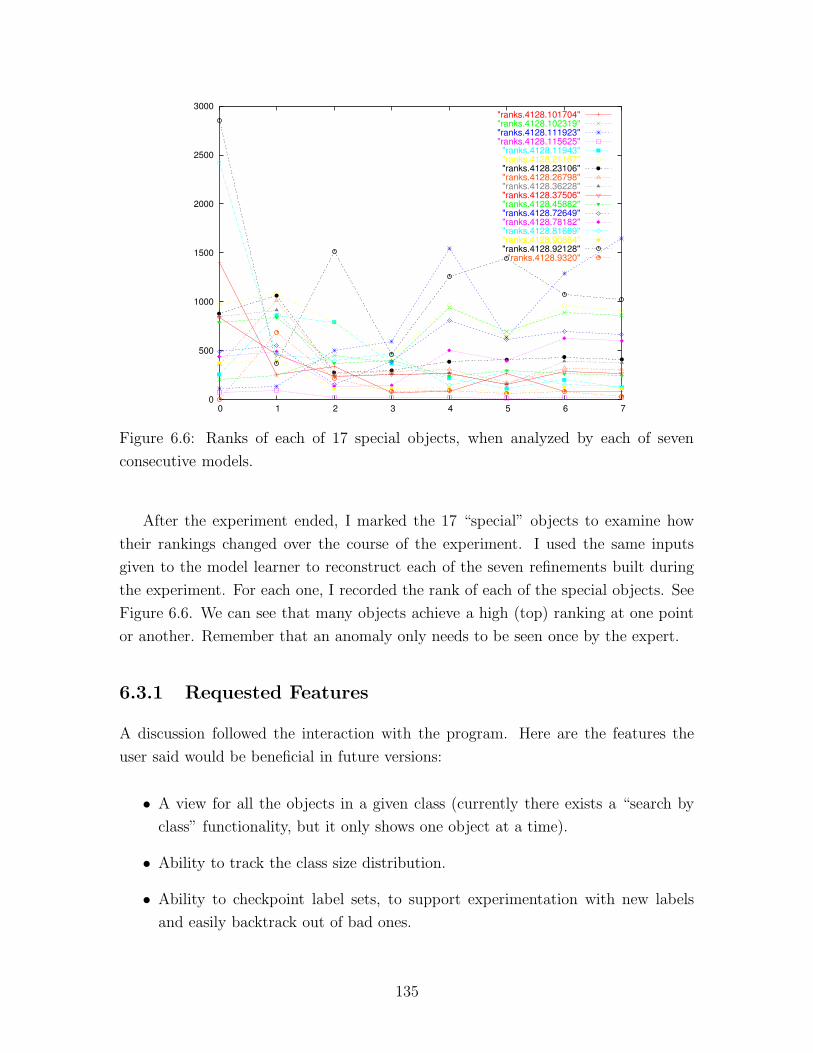
0

500

1000

1500

2000

2500

3000

0 1 2 3 4 5 6 7

"ranks.4128.101704""ranks.4128.102319""ranks.4128.111923""ranks.4128.115625""ranks.4128.11943""ranks.4128.21167""ranks.4128.23106""ranks.4128.26798""ranks.4128.36228""ranks.4128.37506""ranks.4128.45882""ranks.4128.72649""ranks.4128.78182""ranks.4128.81669""ranks.4128.90884""ranks.4128.92128""ranks.4128.9320"

Figure 6.6: Ranks of each of 17 special objects, when analyzed by each of seven

consecutive models.

After the experiment ended, I marked the 17 “special” objects to examine how

their rankings changed over the course of the experiment. I used the same inputs

given to the model learner to reconstruct each of the seven refinements built during

the experiment. For each one, I recorded the rank of each of the special objects. See

Figure 6.6. We can see that many objects achieve a high (top) ranking at one point

or another. Remember that an anomaly only needs to be seen once by the expert.

6.3.1 Requested Features

A discussion followed the interaction with the program. Here are the features the

user said would be beneficial in future versions:

• A view for all the objects in a given class (currently there exists a “search by

class” functionality, but it only shows one object at a time).

• Ability to track the class size distribution.

• Ability to checkpoint label sets, to support experimentation with new labels

and easily backtrack out of bad ones.

135

• The only criterion for displaying an object is its ranking on the anomaly list.

This does not give the user direct control over objects to be excluded. A flag is

needed that would inhibit the display of an object. Presumably such an object

is some kind of boring anomaly that is not being modeled correctly even after

labeling.

• Once a model is built, there needs to be an easy way to carry it over and apply

it to a different data set. For example, a new batch of data from the same source

might be available. It will have the same properties as the existing batch, so

just the anomaly detection phase is needed.

6.4 Conclusion

The anomaly hunting application helps aggregate different kinds of information into

a single view. This, combined with the anomaly finding back-end make it an efficient

way to spot anomalies. Using it, a domain expert was able to spot, within the course of

three hours, anomalies in data set containing half a million objects. By his judgment,

this set includes all of the anomalies in this data. This statement is strengthened by

the plot of object rankings over time and the timeline. Both indicate an overfitting

effect and stabilization of model usefulness before the experiment ended.

When work on this tool started, there was very little support for viewing so much

of the available data in one place. This step was done semi-manually and was time

consuming. Now, new tools like the SkyServer help alleviate this problem. However,

we are unaware of similar ways to incorporate feedback from the expert directly into

the model. In this respect this is a unique tool.

136

Conclusion

I do not claim to have solved the data mining problem. For a start, we still lack a

good definition of that problem. What can be said is that the research community

successfully tackled several different tasks, arrived at crisp definitions for others, and

is still attempting to come up with a grand view of everything. Here, I described a

suite of related subproblems for cluster-based data mining.

It is undeniable that researchers generally have made huge progress in our ability

to mechanically process raw data. This holds for our hardware, software, and mathe-

matical foundations. But an often overlooked fact is that the human ability to grasp

the information as presented did not change. Regardless of how big and complex

the data is, we always need to reduce it to bite-size pieces. For example, traditional

applications of clustering involved hundreds or thousands of biological measurements,

and the output consisted of a (flat or nested) hierarchy of species, with up to a dozen

or two elements. However, modern methods, such as microarrays, require processing

of thousands of different elements, often resulting in complex structures that require

new organization and visualization tools. The same happens in astronomical data,

where scientists now manipulate high-order functions of large scale observations. A

typical reduction in cosmology is processing of tens or hundreds of thousands of ob-

jects into the 2-point correlation function which succinctly describes their structure

(Gray, 2003).

In the future, we can only expect this trend to continue. For instance, plans for

new astronomical surveys call for data collection at the rate of a full SDSS survey

equivalent — currently taking five years to complete — streaming in twice a week.

While we can probably build hardware and software to process this much data in

time, we cannot rely on a new breed of genius scientists to be able to read today’s

output repeated 1000-fold. So a big part of the success of such an endeavor would be

algorithms that can summarize how the universe, as observed last night, is different

from last week’s version.

137

The bottom line is that we are still far from a Grand Unified Theory of data

mining. But we approach it as fast as we can by solving collections of smaller issues,

all seemingly arising from some common need.

Specifically, I concentrate on clustering. Its main advantage is its generality. Sepa-

rating data into groups of similar objects reduces the perception problem significantly.

The classical example is measurements of a population of several hundred crabs. After

clustering, two similar — but different — species can be identified and each specimen

labeled. Published work on the statistical foundations of this kind of modeling dates

back more than 100 years (Pearson, 1894). A huge body of work follows to improve

and expand the methods. Consequently, nowadays we can apply fast methods to sim-

ulate the creation of a universe, and then we can use results such as those presented

here to cluster the resulting millions of galaxies in an attempt to better understand

theories behind dark matter.

Relating back to contributions of this work, my fast K-means algorithm presented

in Chapter 1 gives a two orders of magnitude speedup in low-dimensional data, and

influenced similar works in high dimensions. I extended it into an efficient framework

to choose the number of clusters in Chapter 2. My implementation of both of these

was made available to researchers and was downloaded by over 200 users. It was used

in numerous published and unpublished works. Among them:

• cDNA microarray data. K-means is run repeatedly on a small subset of the

total data (Bainbridge, 2004).

• DNA microarray gene expression levels (Ballini, 2003; Qian, 2001).

• Prediction of functional RNA genes in genomic sequences. The data is clustered

for the purpose of drawing negative examples for the training set. There are

about 700 clusters and more than a million data points (Meraz, 2002).

• Music information retrieval (Logan & Salomon, 2001; Zissimopoulos, 2003).

Multiple features vectors are extracted for each one of 8500 songs. A specialized

inter-cluster distance metric is used to determine a distance matrix for song

similarity.

• Computer program analysis in the Daikon package (Ernst et al., 2001). Likely

invariants for a program are detected dynamically. To determine conditional

properties of the program, X-means clustering is performed on the invariants.

• Computer architecture (Sherwood et al., 2002). A large trace (several billion

instructions) of a computer program is taken. Instructions are grouped into

138

basic blocks. Time intervals of a program’s execution are represented by a

vector of counts of the times each basic block was executed. The vectors are

clustered to determine phases in the program’s execution.

• Natural language processing (Kruengkrai, 2004).

• Financial data analysis (Kallur, 2003).

• Multi-objective optimization with evolutionary algorithms (Koch, 2002).

• Molecular biology (Zhang, 2000).

• Image segmentation (Kruengkrai, 2004).

• Speaker identification.

In Chapter 3 I presented a novel mixture model to produce highly readable clus-

ters. I also show how to fit it efficiently in the EM framework. I gave evidence that it

makes the output of clustering easy for people to comprehend. It was used to aid in

anomaly finding for highway traffic data (Raz et al., 2004). For example, a common

misclassification failure was detected where the low-level software would determine

some trucks had one axle. Another observation made clear was that a system-wide

change occurred around November 1999. Later it was discovered that a vendor of one

of the software components made unreported configuration changes at that date.

In Chapter 4 I applied a “probably approximately correct” approach to dependency-

tree construction for numeric and categorical data. This allows quick processing of

huge inputs with minimal loss of quality. Empirical evidence showed run time which

is constant regardless of the input size, and depends only on intrinsic properties of

the data.

In Chapter 5 I examined the issue of active learning for general mixtures, when

applied to data containing very rare classes of anomalies. I showed that some of

the popular methods for active learning perform poorly in realistic active-learning

scenarios. I also proposed a model-agnostic framework which lets each component

“nominate” its favorite queries, and gave evidence that it is superior to existing

methods. The goal is to quickly find anomalies in large and noisy data sets. The

active-learning “oracle” is a human expert which can tell useful anomalies from plain

errors and known classes of irregularities. The challenge — which was met according

to the empirical evaluation — is accurate classification without over-burdening the

expert.

139

In Chapter 6 I combined principles from Chapters 4 and 5 and presented a graph-

ical application that interacts with a human domain expert to find anomalies in

complex and voluminous data sets. A case study showed its effectiveness on SDSS

data.

In the final anomaly-hunting application, I used only models based on dependency

trees. This does not imply that the other models mentioned cannot be used similarly.

In fact, the active-learning technique described in Chapter 5 is component-agnostic.

The only assumption it makes on the model is that it is a mixture model, with

components that are probability density estimators. It is straightforward to substitute

a K-means component from Chapter 1 or a rectangle-based model from Chapter 3.

In fact, the mixture does not even have to be homogeneous, and can have components

with different forms. The main message is that PDEs that can be estimated from

data can also be combined into mixture models in the EM framework. In addition,

the components are also useful in anomaly detection by appropriate use of the density

function.

This raises the question of which model to use and when. I presented several

different models, and each has its strong and weak points. I now give some rules-of-

thumb to help choose an appropriate model.

• If the data is all numeric, and Euclidean distances in the induced space are

meaningful, K-means is appropriate. Often, different dimensions have hugely

varying ranges. If this is the case then pre-normalization should be performed.

An easy way to do this is the linear transformation to make data in each di-

mension have zero mean and unit variance.

• If the number of clusters is not known in advance, then X-means can help find

it autonomously. Another option is to use the anomaly finding tool to manually

add or remove classes until a reasonable model is generated.

• If human perception of the generated model and the clusters is important, mix-

ture of rectangles is the obvious choice.

• The K-means implementation is the most widely deployed and most robust. It

is also very fast, especially with large numbers of data points and clusters, and

low dimensionality.

• The fast dependency learner is most suited for learning high-dimensional nu-

meric data. It is also appropriate for very large numbers of records.

140

This work opens several avenues for further progress. Below I list several which

promise the most benefit.

• Explore various approaches to the “semi-supervised” learning stage. This is the

part of the anomaly-hunting loop which considers a small set of labeled points

and a much larger unlabeled set to build a PDE.

• Extend the dependency-tree learner so it can handle both continuous and dis-

crete attributes in the same tree.

• Develop an X-means-inspired algorithm for mixtures of Gaussians. Like the

algorithm discussed in Chapter 2, it will perform structure search based on local

decisions. However the mixture components will be generalized Gaussians.

• Investigate alternative approaches to the hint-nomination stage of the anomaly

detector from Chapter 5.

• Accelerate the mixture-of-rectangles algorithm from Chapter 3. The sufficient

statistics needed for the function optimization step are, at most, the one-

dimensional projections of each attribute. It seems possible to leverage this

fact into a fast algorithm. It would also benefit from a public release of the

code so it can be used by researchers.

• Apply the technology introduced in Chapter 4 to the full problem of Bayes Net

structure search.

• Make the fast dependency-tree algorithm in Chapter 4 more disk-access friendly.

This can be achieved by splicing the input into several files, one per attribute,

and keeping a memory buffer of segments of the files.

• Improve the anomaly hunting process from Chapter 6 by incorporating the

suggested improvements identified in the case study. The tool itself is rather

prototypical. Therefore it might be worthwhile to design new tool from scratch.

This also has the advantage of allowing better integration with the data views

and APIs currently offered by the SDSS project’s SkyServer.

• Improve the perceived latency in the anomaly finding stage of the anomaly

hunter tool. Once the user instructs the tool to find anomalies, a set of anomalies

is chosen from a small sample of the data. This sample can be random, but

should also include anomalies previously flagged. Processing of the full data set

will occur in the background. Whenever it finds anomalies better than currently

on display, the front end will be notified and updated.

141

Bibliography

Abazajian, K., Adelman-McCarthy, J., Ageros, M., Allam, S., Anderson, S., & et al(2003). The first data release of the sloan digital sky survey. Astronomical Journal,126.

Agrawal, R., Gehrke, J. E., Gunopulos, D., & Raghavan, P. (1998). Automaticsubspace clustering of high dimensional data for data mining applications. Proc.ACM SIGMOD Int. Conf. Management of Data, 27, 94–105.

AlSabti, K., Ranka, S., & Singh, V. (1999). An efficient space-partitioning basedalgorithm for the K-means clustering. Proceedings of the 3rd Pacific-Asia Con-ference on Methodologies for Knowledge Discovery and Data Mining (PAKDD-99)(pp. 355–359). Berlin: Springer.

Bainbridge, M. (2004). Personal communication.

Ballini, M. (2003). Personal communication.

Baram, Y., El-Yaniv, R., & Luz, K. (2003). Online choice of active learning algo-rithms. Proceedings of the Twentieth International Conference on Machine Learn-ing.

Basu, S., Banerjee, A., & Mooney, R. J. (2004). Active semi-supervision for pairwiseconstrained clustering. Proceedings of the SIAM International Conference on DataMining (SDM-2004). Lake Buena Vista, FL.

Bentley, J. L. (1980). Multidimensional Divide and Conquer. Communications of theACM, 23, 214—229.

Bezdek, J. C. (1981). Pattern recognition with fuzzy objective function algorithms.Plenum Press.

Bishop, C. M. (1995). Neural networks for pattern recognition. Oxford: ClarendonPress.

Blake, C., & Merz, C. (1998). UCI repository of machine learning databases. http://www.ics.uci.edu/∼mlearn/MLRepository.html.

143

Bradley, P. S., & Fayyad, U. M. (1998). Refining initial points for K-Means clustering.Proceedings of the Fifteenth International Conference on Machine Learning (pp. 91–99). Morgan Kaufmann, San Francisco, CA.

Bradley, P. S., Fayyad, U. M., & Reina, C. (1998). Scaling clustering algorithms tolarge databases. Proceedings of the Fourth International Conference on KnowledgeDiscovery and Data Mining (KDD-98) (pp. 9–15). New York: AAAI Press.

Brinker, K. (2003). Incorporating diversity in active learning with support vector ma-chines. Proceedings of the Twentieth International Conference on Machine Learning.

Chow, C. K., & Liu, C. N. (1968). Approximating discrete probability distributionswith dependence trees. IEEE Transactions on Information Theory, 14, 462–467.

Cohn, D., Atlas, L., & Ladner, R. (1994). Improving generalization with activelearning. Machine Learning, 15, 201–221.

Cohn, D. A., Ghahramani, Z., & Jordan, M. I. (1995). Active learning with statisticalmodels. Advances in Neural Information Processing Systems (pp. 705–712). TheMIT Press.

Cormen, T. H., Leiserson, C. E., & Rivest, R. L. (1989). Introduction to algorithms.McGraw-Hill.

Cozman, F. G., Cohen, I., & Cirelo, M. C. (2003). Semi-supervised learning ofmixture models and bayesian networks. Proceedings of the Twentieth InternationalConference on Machine Learning.

Dasgupta, S. (2000). Experiments with random projection. Proceedings of the 16thConference in Uncertainty in Artificial Intelligence (pp. 143–151). San Francisco,CA: Morgan Kaufmann.

Deng, K., & Moore, A. W. (1995). Multiresolution instance-based learning. Proceed-ings of the Twelfth International Joint Conference on Artificial Intelligence (pp.1233–1242). San Francisco: Morgan Kaufmann.

Domingos, P., & Hulten, G. (2000). Mining high-speed data streams. Proceedingsof 6th International Conference on Knowledge Discovery and Data Mining (pp.71–80). N. Y.: ACM Press.

Domingos, P., & Hulten, G. (2001a). A general method for scaling up machinelearning algorithms and its application to clustering. Proceedings of the EighteenthInternational Conference on Machine Learning. Morgan Kaufmann.

Domingos, P., & Hulten, G. (2001b). Learning from infinite data in finite time. Ad-vances in Neural Information Processing Systems 14. Vancouver, British Columbia,Canada.

144

Duda, R. O., & Hart, P. E. (1973). Pattern Classification and Scene Analysis. JohnWiley & Sons.

Elkan, C. (2003). Using the triangle inequality to accelerate k-means. Proceedingsof the Twentieth International Conference on Machine Learning (ICML 2003) (pp.147–153). AAAI Press.

Eppstein, D. (2000). Fast hierarchical clustering and other applications of dynamicclosest pairs. J. Experimental Algorithmics, 5, 1–23.

Ernst, M., Cockrell, J., Griswold, W., & Notkin, D. (2001). Dynamically discoveringlikely program invariants to support program evolution. IEEE Transactions onSoftware Engineering (TSE), 27, 1–25.

Ester, M., Kriegel, H.-P., & Xu, X. (1995). A database interface for clustering inlarge spatial databases. Proceedings of First International Conference on KnowledgeDiscovery and Data Mining. Menlo Park: AAAI.

Farnstrom, F., Lewis, J., & Elkan, C. (2000). Scalability for clustering algorithmsrevisited. SIGKDD Explorations, 2, 51–57.

Fasulo, D. (1999). An analysis of recent work on clustering algorithms. http://

www.cs.washington.edu/homes/dfasulo/clustering.ps.

Friedman, J., & Fisher, N. (1999). Bump hunting in high-dimensional data. Statisticsand Computing, 9, 1–20.

Friedman, N., Goldszmidt, M., & Lee, T. J. (1998). Bayesian Network Classificationwith Continuous Attributes: Getting the Best of Both Discretization and Para-metric Fitting. Proceedings of the Fifteenth International Conference on MachineLearning. Morgan Kaufmann, San Francisco, CA.

Friedman, N., Nachman, I., & Peer, D. (1999). Learning bayesian network struc-ture from massive datasets: The ”sparse candidate” algorithm. Proceedings of the15th Conference on Uncertainty in Artificial Intelligence (UAI-99) (pp. 206–215).Stockholm, Sweden.

Gersho, A., & Gray, R. (1992). Vector quantization and signal compression. KluwerAcademic Publishers; Dordrecht, Netherlands.

Gray, A. (2003). Bringing tractability to generalized n-body problems in statistical andscientific computation. Doctoral dissertation, Carnegie-Mellon University.

Guha, S., Rastogi, R., & Shim, K. (1998). CURE: An efficient clustering algorithmfor large databases. Proceedings of the ACM SIGMOD International Conference onManagement of Data (SIGMOD-98) (pp. 73–84). New York: ACM Press.

Hamerly, G. (2003). Learning structure and concepts in data through data clustering.Doctoral dissertation, University of California, San Diego.

145

Hamerly, G., & Elkan, C. (2002). Alternatives to the k-means algorithm that findbetter clusterings. Proceedings of the 2002 ACM CIKM International Conferenceon Information and Knowledge Management (pp. 600–607). McLean, VA, USA:ACM.

Hamerly, G., & Elkan, C. (2003). Learning the k in k-means. Advances in NeuralInformation Processing Systems 17. MIT Press.

Hettich, S., & Bay, S. D. (1999). The UCI KDD archive. http://kdd.ics.uci.edu.

Hofmann, T., & Buhmann, J. M. (1997). Pairwise data clustering by deterministicannealing. IEEE Transactions on Pattern Analysis and Machine Intelligence, 19,1–14.

Kallur, S. (2003). Personal communication.

Kass, R., & Wasserman, L. (1995). A reference Bayesian test for nested hypothesesand its relationship to the Schwarz criterion. Journal of the American StatisticalAssociation, 90, 773–795.

Kearns, M., Mansour, Y., & Ng, A. Y. (1997). An information-theoretic analysis ofhard and soft assignment methods for clustering. Proceedings of the 13th Conferenceon Uncertainty in Artificial Intelligence (UAI-97) (pp. 282–293). San Francisco:Morgan Kaufmann Publishers.

Koch, T. E. (2002). Personal communication.

Kruengkrai, C. (2004). Personal communication.

LCRS (1998). Las campanas redshift survey. LCRS.http://manaslu.astro.utoronto.ca/∼lin/lcrs.html.

Lewis, D. D., & Catlett, J. (1994). Heterogeneous uncertainty sampling for supervisedlearning. Proceedings of the Eleventh International Conference on Machine Learning(pp. 148–156). New Brunswick, US: Morgan Kaufmann.

Liu, B., Xia, Y., & Yu, P. (2000). Clustering through decision tree construction(Technical Report RC21695). IBM Research.

Logan, B., & Salomon, A. (2001). A music similarity function based on signal analysis.IEEE International Conference on Multimedia and Expo.

Maass, W., & Warmuth, M. K. (1995). Efficient learning with virtual threshold gates.Proc. 12th International Conference on Machine Learning (pp. 378–386). MorganKaufmann.

MacKay, D. (1992). Information-based objective functions for active data selection.Neural Computation, 4, 590–604.

146

Maron, O., & Moore, A. W. (1994). Hoeffding races: Accelerating model selectionsearch for classification and function approximation. Advances in Neural Informa-tion Processing Systems (pp. 59–66). Denver, Colorado: Morgan Kaufmann.

Mehta, M., Agrawal, R., & Rissanen, J. (1996). SLIQ: A fast scalable classifier fordata mining. 5th Intl. Conf. on Extending Database Technology.

Meila, M. (1999a). An accelerated chow and liu algorithm: fitting tree distributions tohigh dimensional sparse data. Proceedings of the Sixteenth International Conferenceon Machine Learning.

Meila, M. (1999b). Learning with mixtures of trees. Doctoral dissertation, Mas-sachusetts Institute of Technology.

Meila, M., & Heckerman, D. (1998). An experimental comparison of several clusteringand initilalization methods (Technical Report 98-06). Microsoft Research, Redmond,WA.

Meraz, R. (2002). Personal communication.

Miller, D. J., & Uyar, H. S. (1997). A mixture of experts classifier with learning basedon both labeled and unlabelled data. Advances in Neural Information ProcessingSystems 9.

Moore, A. (1998). Very fast EM-based mixture model clustering using multiresolutionkd-trees. Advances in Neural Information Processing Systems 10 (pp. 543–549).Morgan Kaufmann.

Moore, A. (2000). The anchors hierarchy: Using the triangle inequality to survive highdimensional data. Proceedings of the 16th Conference on Uncertainty in ArtificialIntelligence (pp. 397–405). San Francisco, CA: Morgan Kaufmann.

Moore, A. W. (1991). Efficient memory-based learning for robot control. Doctoraldissertation, University of Cambridge. Technical Report 209, Computer Laboratory,University of Cambridge.

Moore, A. W., & Lee, M. S. (1994). Efficient algorithms for minimizing cross val-idation error. Proceedings of the Eleventh International Conference on MachineLearning (pp. 190–198). New Brunswick, US: Morgan Kaufmann.

Moore, A. W., & Lee, M. S. (1998). Cached sufficient statistics for efficient machinelearning with large datasets. Journal of Artificial Intelligence Research, 8, 67–91.

Nagesh, H., Goil, S., & Choudhary, A. (1999). MAFIA: Efficient and scalable sub-space clustering for very large data sets (Technical Report 9906-010). NorthwesternUniversity.

Ng, R. T., & Han, J. (1994). Efficient and effective clustering methods for spatialdata mining. Proceedings of VLDB.

147

Nichol, R. C., Collins, C. A., & Lumsden, S. L. (2000). The Edinburgh/Durhamsouthern galaxy catalogue — IX. Submitted to the Astrophysical Journal.

P.Brazdil, & J.Gama (1991). StatLog. http://www.liacc.up.pt/ML/statlog.

Pearson, K. (1894). Contributions to the mathematical theory of evolution. Philo-sophical Transaction A, 185, 71–110.

Pelleg, D. (2003). Hunting anomalies in sloan data. Proc. 7th Great Lakes CosmologyWorkshop.

Pelleg, D., & Moore, A. (1999). Accelerating exact k-means algorithms with geometricreasoning. Proceedings of the Fifth ACM SIGKDD International Conference onKnowledge Discovery and Data Mining (pp. 277–281). New York, NY: AAAI Press.An extended version is available as Technical Report CMU-CS-00-105.

Pelleg, D., & Moore, A. (2000a). Accelerating exact k-means with geometric reasoning(Technical Report CMU-CS-00-105). Carnegie Mellon University. Also availablefrom http://www.cs.cmu.edu/∼dpelleg/.

Pelleg, D., & Moore, A. (2000b). X-means: Extending K-means with efficient estima-tion of the number of clusters. Proc. 17th International Conf. on Machine Learning(pp. 727–734). Morgan Kaufmann, San Francisco, CA.

Pelleg, D., & Moore, A. (2001). Mixtures of rectangles: Interpretable soft cluster-ing. Proc. 18th International Conf. on Machine Learning (pp. 401–408). MorganKaufmann, San Francisco, CA.

Pelleg, D., & Moore, A. (2002). Using Tarjan’s red rule for fast dependency treeconstruction. Advances in Neural Information Processing Systems 15 (pp. 801–808). Cambridge, MA: MIT Press.

Plutowski, M., & White, H. (1993). Selecting concise training sets from clean data.IEEE Transactions on Neural Networks, 4, 305–318.

Press, W. H., Teukolsky, S. A., Vetterling, W. T., & Flannery, B. P. (1992). Numericalrecipes in C, 2nd. edition. Cambridge University Press.

Qian, Y. (2001). Personal communication.

Raz, O., Buchheit, R., Shaw, M., Koopman, P., & Faloutsos, C. (2004). Detectingsemantic anomalies in truck weigh-in-motion traffic data using data mining. Journalof Computing in Civil Engineering.

Reza, F. (1994). An introduction to information theory, 282–283. New York: DoverPublications.

SDSS (1998). The sloan digital sky survey. SDSS. www.sdss.org.

148

Seeger, M. (2000). Learning with labeled and unlabeled data (Technical Report). In-stitue for Adaptive and Neural Computation, University of Edinburgh.

Seung, H. S., Opper, M., & Sompolinsky, H. (1992). Query by committee. Computa-tional Learning Theory (pp. 287–294).

Shafer, J. C., Agrawal, R., & Mehta, M. (1996). SPRINT: A scalable parallel classifierfor data mining. Proc. 22nd Int. Conf. Very Large Databases (pp. 544–555). Mumbai(Bombay), India: Morgan Kaufmann.

Shahshashani, B., & Landgrebe, D. A. (1994). The effect of unlabeled examplesin reducing the small sample size problem. IEEE Trans Geoscience and RemoteSensing, 32, 1087–1095.

Sherwood, T., Perelman, E., Hamerly, G., & Calder, B. (2002). Automatically char-acterizing large scale program behavior. 10th International Conference on Archi-tectural Support for Programming Languages and Operating Systems.

Stephens, M. A. (1974). EDF statistics for goodness of fit and some comparisons.Journal of the American Statistical Association, 69, 730–737.

Szalay, A., Gray, J., Thakar, A., Boroski, B., Gal, R., Li, N., Kunszt, P., Ma-lik, T., O’Mullane, W., Nieto-Santisteban, M., Raddick, J., Stoughton, C., &vandenBerg, J. (2004). The SDSS DR1 skyserver. To be published. http://

skyserver.sdss.org/.

Tarjan, R. E. (1983). Data structures and network algorithms, vol. 44 of CBMS-NSFReg. Conf. Ser. Appl. Math. SIAM.

Ueda, N., & Nakano, R. (1998). Deterministic annealing em algorithm. NeuralNetworks, 11, 271–282.

Wasserman, L. (1997). Bayesian model selection and model averaging (TechnicalReport TR666). Carnegie Mellon University, Pittsburgh, PA. Also available fromhttp://www.stat.cmu.edu/www/cmu-stats/tr/tr666/tr666.html.

Wiratunga, N., Craw, S., & Massie, S. (2003). Index driven selective sampling forCBR. Proceedings of the Fifth International Conference on Case-Based Reasoning.Trondheim, Norway: Springer-Verlag.

Witten, I. H., & Frank, E. (2000). Data mining: Practical machine learning toolswith java implementations. San Francisco: Morgan Kaufmann.

Zhang, B., Hsu, M., & Dayal, U. (2000). K-harmonic means - a data clusteringalgorithm (Technical Report). Hewlett-Packard Labs.

Zhang, M. (2000). Personal communication.

Zhang, T., Ramakrishnan, R., & Livny, M. (1995). BIRCH: An efficient data cluster-ing method for very large databases,. Proceedings of ACM SIGMOD (pp. 103–114).

149

Zissimopoulos, B. (2003). Personal communication.

150

Scalable and Practical Probability Density Estimators for ...

Documents

Transcript of Scalable and Practical Probability Density Estimators for ...