SAS Scalable Performance Data Server 5.1: User's Guide, Second
330
SAS ® Scalable Performance Data Server 5.1 User’s Guide Second Edition SAS ® Documentation
Transcript of SAS Scalable Performance Data Server 5.1: User's Guide, Second

SAS® Scalable Performance Data Server 5.1 User’s GuideSecond Edition
SAS® Documentation

The correct bibliographic citation for this manual is as follows: SAS Institute Inc. 2013. SAS® Scalable Performance Data Server 5.1: User’s Guide, Second Edition. Cary, NC : SAS Institute Inc.
SAS® Scalable Performance Data Server 5.1: User's Guide, Second Edition
Copyright © 2013, SAS Institute Inc., Cary, NC, USA
All rights reserved. Produced in the United States of America.
For a hardcopy book: No part of this publication may be reproduced, stored in a retrieval system, or transmitted, in any form or by any means, electronic, mechanical, photocopying, or otherwise, without the prior written permission of the publisher, SAS Institute Inc.
For a Web download or e-book:Your use of this publication shall be governed by the terms established by the vendor at the time you acquire this publication.
The scanning, uploading, and distribution of this book via the Internet or any other means without the permission of the publisher is illegal and punishable by law. Please purchase only authorized electronic editions and do not participate in or encourage electronic piracy of copyrighted materials. Your support of others' rights is appreciated.
U.S. Government License Rights; Restricted Rights: Use, duplication, or disclosure of this software and related documentation by the U.S. government is subject to the Agreement with SAS Institute and the restrictions set forth in FAR 52.227–19 Commercial Computer Software-Restricted Rights (June 1987).
SAS Institute Inc., SAS Campus Drive, Cary, North Carolina 27513.
Electronic book 1, December 2013
SAS® Publishing provides a complete selection of books and electronic products to help customers use SAS software to its fullest potential. For more information about our e-books, e-learning products, CDs, and hard-copy books, visit the SAS Publishing Web site at support.sas.com/publishing or call 1-800-727-3228.
SAS® and all other SAS Institute Inc. product or service names are registered trademarks or trademarks of SAS Institute Inc. in the USA and other countries. ® indicates USA registration.
Other brand and product names are registered trademarks or trademarks of their respective companies.


Contents
PART 1 Product Notes 1
Chapter 1 • What’s New in SAS Scalable Performance Data (SPD) Server 5.1 . . . . . . . . . . . . . . 3What’s New in SPD Server 5.1? . . . . . . . . . . . . . . . . . . . . . . . . . . . . . . . . . . . . . . . . . . . . 3
PART 2 Using SAS Scalable Performance Data (SPD) Server 5
Chapter 2 • Overview of SAS Scalable Performance Data (SPD) Server . . . . . . . . . . . . . . . . . . . 7Overview of SAS Scalable Performance Data (SPD) Server . . . . . . . . . . . . . . . . . . . . . . 7The SPD Server Client/Server Model . . . . . . . . . . . . . . . . . . . . . . . . . . . . . . . . . . . . . . . . 8Accessing SPD Server Using SAS . . . . . . . . . . . . . . . . . . . . . . . . . . . . . . . . . . . . . . . . . 10Securing SAS Data . . . . . . . . . . . . . . . . . . . . . . . . . . . . . . . . . . . . . . . . . . . . . . . . . . . . . 11SPD Server Extensions to Base SAS . . . . . . . . . . . . . . . . . . . . . . . . . . . . . . . . . . . . . . . 12
Chapter 3 • Connecting to SAS Scalable Performance Data (SPD) Server . . . . . . . . . . . . . . . . . 13Introduction . . . . . . . . . . . . . . . . . . . . . . . . . . . . . . . . . . . . . . . . . . . . . . . . . . . . . . . . . . . 13Accessing SPD Server from a SAS Client . . . . . . . . . . . . . . . . . . . . . . . . . . . . . . . . . . . 13SPD Server Table Options . . . . . . . . . . . . . . . . . . . . . . . . . . . . . . . . . . . . . . . . . . . . . . . 18
Chapter 4 • Accessing and Creating SAS Scalable Performance Data (SPD) Server Tables . . 19SAS and SPD Server Tables . . . . . . . . . . . . . . . . . . . . . . . . . . . . . . . . . . . . . . . . . . . . . . 19SPD Server Resource Security . . . . . . . . . . . . . . . . . . . . . . . . . . . . . . . . . . . . . . . . . . . . 20Using a LIBNAME Statement to Access SPD Server . . . . . . . . . . . . . . . . . . . . . . . . . . 21Managing Large SPD Server Files . . . . . . . . . . . . . . . . . . . . . . . . . . . . . . . . . . . . . . . . . 22Migrating Tables between SAS and SPD Server . . . . . . . . . . . . . . . . . . . . . . . . . . . . . . 22Accessing and Manipulating Data with the SQL Pass-Through Facility . . . . . . . . . . . . 24Creating a New Table . . . . . . . . . . . . . . . . . . . . . . . . . . . . . . . . . . . . . . . . . . . . . . . . . . . 28
Chapter 5 • Indexing, Sorting, and Manipulating SAS Scalable Performance Data (SPD) Server Tables . . . . . . . . . . . . . . . . . . . . . . . . . . . . . . . . . . . . . . . . . . . . . . . . . . . . . . 31
Indexing Tables . . . . . . . . . . . . . . . . . . . . . . . . . . . . . . . . . . . . . . . . . . . . . . . . . . . . . . . 31Examples of Creating SPD Server Indexes . . . . . . . . . . . . . . . . . . . . . . . . . . . . . . . . . . 31
Chapter 6 • SAS Scalable Performance Data (SPD) Server Dynamic Cluster Tables . . . . . . . . 35Overview of Dynamic Cluster Tables . . . . . . . . . . . . . . . . . . . . . . . . . . . . . . . . . . . . . . 36Dynamic Cluster Table Structure . . . . . . . . . . . . . . . . . . . . . . . . . . . . . . . . . . . . . . . . . . 36Benefits of Dynamic Cluster Tables . . . . . . . . . . . . . . . . . . . . . . . . . . . . . . . . . . . . . . . . 37Dynamic Cluster Table Operations . . . . . . . . . . . . . . . . . . . . . . . . . . . . . . . . . . . . . . . . 38Dynamic Cluster BY Clause Optimization . . . . . . . . . . . . . . . . . . . . . . . . . . . . . . . . . . . 49Member Table Requirements for Creating Dynamic Cluster Tables . . . . . . . . . . . . . . . 52Querying and Reading Member Tables in a Dynamic Cluster . . . . . . . . . . . . . . . . . . . . 55Unsupported Features in Dynamic Cluster Tables . . . . . . . . . . . . . . . . . . . . . . . . . . . . . 57Dynamic Cluster Table Examples . . . . . . . . . . . . . . . . . . . . . . . . . . . . . . . . . . . . . . . . . 57

PART 3 SAS Scalable Performance Data (SPD) Server SQL Features 65
Chapter 7 • SAS Scalable Performance Data (SPD) Server SQL Features . . . . . . . . . . . . . . . . . 67Differences between SAS SQL and SPD Server SQL . . . . . . . . . . . . . . . . . . . . . . . . . . 69Connecting to the SPD Server SQL Engine . . . . . . . . . . . . . . . . . . . . . . . . . . . . . . . . . . 70Specifying SPD Server SQL Planner Options . . . . . . . . . . . . . . . . . . . . . . . . . . . . . . . . 71Important SPD Server SQL Planner Options . . . . . . . . . . . . . . . . . . . . . . . . . . . . . . . . . 72Parallel Join Facility . . . . . . . . . . . . . . . . . . . . . . . . . . . . . . . . . . . . . . . . . . . . . . . . . . . . 80Parallel Group-By Facility . . . . . . . . . . . . . . . . . . . . . . . . . . . . . . . . . . . . . . . . . . . . . . . 83Parallel Group-By SQL Reset Options . . . . . . . . . . . . . . . . . . . . . . . . . . . . . . . . . . . . . . 87SPD Server STARJOIN Facility . . . . . . . . . . . . . . . . . . . . . . . . . . . . . . . . . . . . . . . . . . 88STARJOIN RESET Statement Options . . . . . . . . . . . . . . . . . . . . . . . . . . . . . . . . . . . . . 93SPD Server STARJOIN Examples . . . . . . . . . . . . . . . . . . . . . . . . . . . . . . . . . . . . . . . . . 95SPD Server Join Planner . . . . . . . . . . . . . . . . . . . . . . . . . . . . . . . . . . . . . . . . . . . . . . . . . 97SPD Server Index Scan . . . . . . . . . . . . . . . . . . . . . . . . . . . . . . . . . . . . . . . . . . . . . . . . . . 97Optimizing Correlated Queries . . . . . . . . . . . . . . . . . . . . . . . . . . . . . . . . . . . . . . . . . . . 100Correlated Query Options . . . . . . . . . . . . . . . . . . . . . . . . . . . . . . . . . . . . . . . . . . . . . . . 100SPD Server SQL Views . . . . . . . . . . . . . . . . . . . . . . . . . . . . . . . . . . . . . . . . . . . . . . . . 102SPD Server SQL Extensions . . . . . . . . . . . . . . . . . . . . . . . . . . . . . . . . . . . . . . . . . . . . 106SPD Server SQL Cluster Operations . . . . . . . . . . . . . . . . . . . . . . . . . . . . . . . . . . . . . . 113
PART 4 SAS Scalable Performance Data (SPD) Server Reference 117
Chapter 8 • Optimizing SAS Scalable Performance Data Server (SPD) Server . . . . . . . . . . . . 119SPD Server Performance and Usage Tips . . . . . . . . . . . . . . . . . . . . . . . . . . . . . . . . . . 120Symmetric Multiple Processor (SMP) Utilization . . . . . . . . . . . . . . . . . . . . . . . . . . . . 120File System Performance Concepts . . . . . . . . . . . . . . . . . . . . . . . . . . . . . . . . . . . . . . . 121LIBNAME Domains . . . . . . . . . . . . . . . . . . . . . . . . . . . . . . . . . . . . . . . . . . . . . . . . . . . 123Loading Data into an SPD Server Host . . . . . . . . . . . . . . . . . . . . . . . . . . . . . . . . . . . . 124Table Loading Techniques . . . . . . . . . . . . . . . . . . . . . . . . . . . . . . . . . . . . . . . . . . . . . . 125Loading Indexes in Parallel . . . . . . . . . . . . . . . . . . . . . . . . . . . . . . . . . . . . . . . . . . . . . 127Truncating Tables . . . . . . . . . . . . . . . . . . . . . . . . . . . . . . . . . . . . . . . . . . . . . . . . . . . . . 128Optimizing WHERE Clauses . . . . . . . . . . . . . . . . . . . . . . . . . . . . . . . . . . . . . . . . . . . . 129SPD Server Indexing . . . . . . . . . . . . . . . . . . . . . . . . . . . . . . . . . . . . . . . . . . . . . . . . . . 130WHERE Clause Planner . . . . . . . . . . . . . . . . . . . . . . . . . . . . . . . . . . . . . . . . . . . . . . . . 133How to Affect the WHERE Planner . . . . . . . . . . . . . . . . . . . . . . . . . . . . . . . . . . . . . . . 139Identical Parallel WHERE Clause Subsetting Results . . . . . . . . . . . . . . . . . . . . . . . . . 141WHERE Clause Examples . . . . . . . . . . . . . . . . . . . . . . . . . . . . . . . . . . . . . . . . . . . . . . 144Server-Side Sorting . . . . . . . . . . . . . . . . . . . . . . . . . . . . . . . . . . . . . . . . . . . . . . . . . . . . 149
Chapter 9 • SAS Scalable Performance Data (SPD) Server Macro Variables . . . . . . . . . . . . . . 151Introduction . . . . . . . . . . . . . . . . . . . . . . . . . . . . . . . . . . . . . . . . . . . . . . . . . . . . . . . . . . 152Variable for Compatibility with the Base SAS Engine . . . . . . . . . . . . . . . . . . . . . . . . 152Variables for Miscellaneous Functions . . . . . . . . . . . . . . . . . . . . . . . . . . . . . . . . . . . . 153Variables for Sorts . . . . . . . . . . . . . . . . . . . . . . . . . . . . . . . . . . . . . . . . . . . . . . . . . . . . 158Variables for WHERE Clause Evaluations . . . . . . . . . . . . . . . . . . . . . . . . . . . . . . . . . 160Variables That Affect Disk Space . . . . . . . . . . . . . . . . . . . . . . . . . . . . . . . . . . . . . . . . 166Variables to Enhance Performance . . . . . . . . . . . . . . . . . . . . . . . . . . . . . . . . . . . . . . . . 169Variable for a Client and a Server Running on the Same UNIX Machine . . . . . . . . . . 171
Chapter 10 • SAS Scalable Performance Data (SPD) Server LIBNAME Options . . . . . . . . . . . 173
vi Contents
Introduction . . . . . . . . . . . . . . . . . . . . . . . . . . . . . . . . . . . . . . . . . . . . . . . . . . . . . . . . . . 173Options to Locate an SPD Server Host . . . . . . . . . . . . . . . . . . . . . . . . . . . . . . . . . . . . . 174Options to Identify the SPD Server Client . . . . . . . . . . . . . . . . . . . . . . . . . . . . . . . . . . 175Options to Specify Implicit SQL Pass-Through . . . . . . . . . . . . . . . . . . . . . . . . . . . . . . 180Options for Access Control Lists (ACLs) . . . . . . . . . . . . . . . . . . . . . . . . . . . . . . . . . . 181Options for a Client and Server Running on the Same UNIX Machine . . . . . . . . . . . . 182Options for Other Functions . . . . . . . . . . . . . . . . . . . . . . . . . . . . . . . . . . . . . . . . . . . . . 183
Chapter 11 • SAS Scalable Performance Data (SPD) Server Table Options . . . . . . . . . . . . . . . 193Introduction . . . . . . . . . . . . . . . . . . . . . . . . . . . . . . . . . . . . . . . . . . . . . . . . . . . . . . . . . . 193Option for Compatibility with Base SAS Software . . . . . . . . . . . . . . . . . . . . . . . . . . . 194Options That Affect Disk Space . . . . . . . . . . . . . . . . . . . . . . . . . . . . . . . . . . . . . . . . . . 195Options to Enhance Performance . . . . . . . . . . . . . . . . . . . . . . . . . . . . . . . . . . . . . . . . . 197Option to Test Performance . . . . . . . . . . . . . . . . . . . . . . . . . . . . . . . . . . . . . . . . . . . . . 200Options for WHERE Clause Evaluations . . . . . . . . . . . . . . . . . . . . . . . . . . . . . . . . . . . 201Options for Other Functions . . . . . . . . . . . . . . . . . . . . . . . . . . . . . . . . . . . . . . . . . . . . . 206Options for Security . . . . . . . . . . . . . . . . . . . . . . . . . . . . . . . . . . . . . . . . . . . . . . . . . . . 216
Chapter 12 • SAS Scalable Performance Data (SPD) Server Formats and Informats . . . . . . . 219Introduction . . . . . . . . . . . . . . . . . . . . . . . . . . . . . . . . . . . . . . . . . . . . . . . . . . . . . . . . . . 219Formats . . . . . . . . . . . . . . . . . . . . . . . . . . . . . . . . . . . . . . . . . . . . . . . . . . . . . . . . . . . . . 219User-Defined Formats . . . . . . . . . . . . . . . . . . . . . . . . . . . . . . . . . . . . . . . . . . . . . . . . . 221Informats . . . . . . . . . . . . . . . . . . . . . . . . . . . . . . . . . . . . . . . . . . . . . . . . . . . . . . . . . . . . 225
Chapter 13 • SAS Scalable Performance Data (SPD) Server NLS Support . . . . . . . . . . . . . . . . 229Overview of NLS . . . . . . . . . . . . . . . . . . . . . . . . . . . . . . . . . . . . . . . . . . . . . . . . . . . . . 229Character Encoding . . . . . . . . . . . . . . . . . . . . . . . . . . . . . . . . . . . . . . . . . . . . . . . . . . . 230Moving Data across Environments with Different Encodings . . . . . . . . . . . . . . . . . . . 233Base SAS Encoding Behavior . . . . . . . . . . . . . . . . . . . . . . . . . . . . . . . . . . . . . . . . . . . 234Setting the Encoding for Base SAS Sessions . . . . . . . . . . . . . . . . . . . . . . . . . . . . . . . . 235Changing the Encoding for Base SAS Sessions . . . . . . . . . . . . . . . . . . . . . . . . . . . . . . 236NLS Support in SPD Server . . . . . . . . . . . . . . . . . . . . . . . . . . . . . . . . . . . . . . . . . . . . . 237
Chapter 14 • Using SAS Scalable Performance Data (SPD) Server with Other Clients . . . . . . 241Overview of Using SPD Server with Other Clients . . . . . . . . . . . . . . . . . . . . . . . . . . . 241Using Open Database Connectivity (ODBC) to Access SPD Server Tables . . . . . . . . 242Using JDBC (Java) to Access SPD Server Tables . . . . . . . . . . . . . . . . . . . . . . . . . . . . 247
Chapter 15 • SAS Scalable Performance Data (SPD) Server SQL Access Library API Reference . . . . . . . . . . . . . . . . . . . . . . . . . . . . . . . . . . . . . . . . . . . . . . . . . . . . . . . 251
Introduction . . . . . . . . . . . . . . . . . . . . . . . . . . . . . . . . . . . . . . . . . . . . . . . . . . . . . . . . . . 251Overview of SPQL Usage . . . . . . . . . . . . . . . . . . . . . . . . . . . . . . . . . . . . . . . . . . . . . . 252SPQL API Description . . . . . . . . . . . . . . . . . . . . . . . . . . . . . . . . . . . . . . . . . . . . . . . . . 252SPQL API Functions . . . . . . . . . . . . . . . . . . . . . . . . . . . . . . . . . . . . . . . . . . . . . . . . . . 252SPQL Function Return Codes . . . . . . . . . . . . . . . . . . . . . . . . . . . . . . . . . . . . . . . . . . . 256
PART 5 SPD Server Appendices 259
Appendix 1 • SPD Server Advanced User Topics . . . . . . . . . . . . . . . . . . . . . . . . . . . . . . . . . . . . 261SPD Server Advanced User Topics . . . . . . . . . . . . . . . . . . . . . . . . . . . . . . . . . . . . . . . 262Accessing SPD Server through SAS . . . . . . . . . . . . . . . . . . . . . . . . . . . . . . . . . . . . . . 262Organizing SAS Data . . . . . . . . . . . . . . . . . . . . . . . . . . . . . . . . . . . . . . . . . . . . . . . . . . 265SPD Server Performance Enhancements . . . . . . . . . . . . . . . . . . . . . . . . . . . . . . . . . . . 267Using SPD Server with Data Warehousing . . . . . . . . . . . . . . . . . . . . . . . . . . . . . . . . . 268
Contents vii
SPD Server Macro Variables . . . . . . . . . . . . . . . . . . . . . . . . . . . . . . . . . . . . . . . . . . . . 270Using a LIBNAME to Statement to Access SPD Server . . . . . . . . . . . . . . . . . . . . . . . 270Managing Large SPD Server Files . . . . . . . . . . . . . . . . . . . . . . . . . . . . . . . . . . . . . . . . 272Indexing SPD Server Tables . . . . . . . . . . . . . . . . . . . . . . . . . . . . . . . . . . . . . . . . . . . . . 277SPD Server Join Planner . . . . . . . . . . . . . . . . . . . . . . . . . . . . . . . . . . . . . . . . . . . . . . . . 278SPD Server Join Planner Examples . . . . . . . . . . . . . . . . . . . . . . . . . . . . . . . . . . . . . . . 279SPD Server STARJOIN Optimization . . . . . . . . . . . . . . . . . . . . . . . . . . . . . . . . . . . . . 281
Appendix 2 • SAS Scalable Performance Data (SPD) Server Frequently Asked Questions . . 287
Appendix 3 • SAS Scalable Performance Data (SPD) Server SQL Syntax Reference Guide . 305SPD Server SQL Syntax . . . . . . . . . . . . . . . . . . . . . . . . . . . . . . . . . . . . . . . . . . . . . . . . 306Document Conventions . . . . . . . . . . . . . . . . . . . . . . . . . . . . . . . . . . . . . . . . . . . . . . . . 306SQL Syntax Definitions . . . . . . . . . . . . . . . . . . . . . . . . . . . . . . . . . . . . . . . . . . . . . . . . 306SQL Statements . . . . . . . . . . . . . . . . . . . . . . . . . . . . . . . . . . . . . . . . . . . . . . . . . . . . . . 308SQL Building Blocks . . . . . . . . . . . . . . . . . . . . . . . . . . . . . . . . . . . . . . . . . . . . . . . . . . 312
Appendix 4 • SPD Server Supported SQL and WHERE-Processing Functions . . . . . . . . . . . . 319
viii Contents
Part 1
Product Notes
Chapter 1What’s New in SAS Scalable Performance Data (SPD) Server 5.1 . . . 3
1

2
Chapter 1
What’s New in SAS Scalable Performance Data (SPD) Server 5.1
What’s New in SPD Server 5.1? . . . . . . . . . . . . . . . . . . . . . . . . . . . . . . . . . . . . . . . . . . 3
What’s New in SPD Server 5.1?SAS 9.4 includes a new SPD Server engine client that can connect with the SPD Server 5.1 server. SPD Server 5.1 also offers expanded support for regulatory, IT, and end user features such as the following:
• Enhanced (AES-256) encryption for data at rest
• Windows 64-bit server support
• SQL performance enhancements
• New SPD Server cluster features introduce enhanced operation, including functions for Cluster Remove, Cluster Replace, and online cluster management.
• New dictionary table types in SQL enables you to view SPD Server cluster and system information.
• Join planner enhancements and hash join optimizations.
• Now supports up to 32 groups per user.
• Validates the paths to the start-up files libnames.parm and spdsserv.parm.
• Enabled prxmatch() support for PERL regular expression pattern matching and support in SPD Server WHERE clauses.
• Information is generated that enables SPD Server administrators to identify the SPD Server user who spawned a given spdsbase processes.
• Binary compression.
3

4 Chapter 1 • What’s New in SAS Scalable Performance Data (SPD) Server 5.1

Part 2
Using SAS Scalable Performance Data (SPD) Server
Chapter 2Overview of SAS Scalable Performance Data (SPD) Server . . . . . . . . 7
Chapter 3Connecting to SAS Scalable Performance Data (SPD) Server . . . . . 13
Chapter 4Accessing and Creating SAS Scalable Performance Data (SPD) Server Tables . . . . . . . . . . . . . . . . . . . . . . . . . . . 19
Chapter 5Indexing, Sorting, and Manipulating SAS Scalable Performance Data (SPD) Server Tables . . . . . . . . . . . . . . . . . . . . . . . . . . . 31
Chapter 6SAS Scalable Performance Data (SPD) Server Dynamic Cluster Tables . . . . . . . . . . . . . . . . . . . . . . . . . . . . . . . . . . . . . . . . . . 35
5

6
Chapter 2
Overview of SAS Scalable Performance Data (SPD) Server
Overview of SAS Scalable Performance Data (SPD) Server . . . . . . . . . . . . . . . . . . . 7
The SPD Server Client/Server Model . . . . . . . . . . . . . . . . . . . . . . . . . . . . . . . . . . . . . . 8Overview of the Client/Server Model . . . . . . . . . . . . . . . . . . . . . . . . . . . . . . . . . . . . . 8Symmetric Multiprocessor Hosts . . . . . . . . . . . . . . . . . . . . . . . . . . . . . . . . . . . . . . . . 9SPD Server Host Services for Clients . . . . . . . . . . . . . . . . . . . . . . . . . . . . . . . . . . . . 9
Accessing SPD Server Using SAS . . . . . . . . . . . . . . . . . . . . . . . . . . . . . . . . . . . . . . . . 10SQL Pass-Through Facility . . . . . . . . . . . . . . . . . . . . . . . . . . . . . . . . . . . . . . . . . . . 10
Securing SAS Data . . . . . . . . . . . . . . . . . . . . . . . . . . . . . . . . . . . . . . . . . . . . . . . . . . . . 11Registering the LIBNAME Domain . . . . . . . . . . . . . . . . . . . . . . . . . . . . . . . . . . . . . 11ACL File Security . . . . . . . . . . . . . . . . . . . . . . . . . . . . . . . . . . . . . . . . . . . . . . . . . . . 11
SPD Server Extensions to Base SAS . . . . . . . . . . . . . . . . . . . . . . . . . . . . . . . . . . . . . . 12
Overview of SAS Scalable Performance Data (SPD) Server
SPD Server software is designed for high-performance data delivery. Its primary function is to provide user access to SAS data for intensive processing (queries and sorts) on the host server machine. When client workstations on different platforms send processing requests to an SPD Server host, the host returns results in the format required by each client workstation.
SPD Server uses parallelism to deliver rapid results for each user, while supporting many simultaneous users.
SPD Server 5.1 provides on-disk structures that are compatible with SAS 9.4 and the large table capacities that it supports. SPD Server clusters are a unique design feature. SPD Server is a full 64-bit server that supports up to 2 billion columns and for all practical purposes, unlimited rows of data.
SPD Server 5.1 operates on computers running SAS 9.4 or later. PC users who do not use SAS can still use SPD Server. For more information about connecting to SPD Server, see “Overview of Using SPD Server with Other Clients” on page 241. SAS users can access SPD Server by using SQL pass-through or by using the SAS language.
Syntax Conventions: SPD Server software supports SAS users and other users. SPD Server documentation uses common terminology that both audiences should understand. In SPD Server documentation, SAS data sets are referred to as tables, SAS variables are referred to as columns, and SAS observations are referred to as rows. The SPD Server
7
product is referred to as SPD Server or the software, depending on the context of the documentation.
The SPD Server Client/Server Model
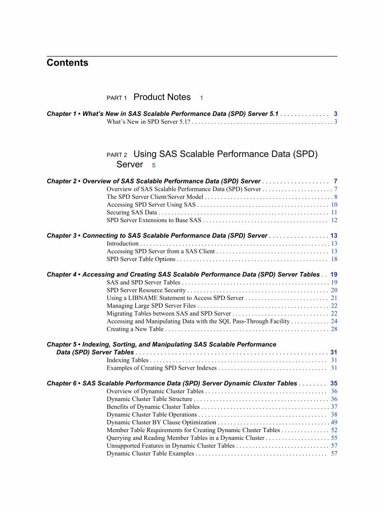
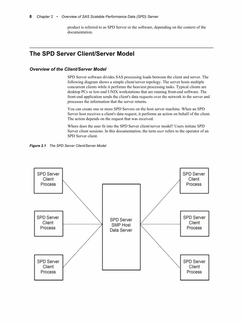
Overview of the Client/Server ModelSPD Server software divides SAS processing loads between the client and server. The following diagram shows a simple client/server topology. The server hosts multiple concurrent clients while it performs the heaviest processing tasks. Typical clients are desktop PCs or low-end UNIX workstations that are running front-end software. The front-end application sends the client's data requests over the network to the server and processes the information that the server returns.
You can create one or more SPD Servers on the host server machine. When an SPD Server host receives a client's data request, it performs an action on behalf of the client. The action depends on the request that was received.
Where does the user fit into the SPD Server client/server model? Users initiate SPD Server client sessions. In this documentation, the term user refers to the operator of an SPD Server client.
Figure 2.1 The SPD Server Client/Server Model
8 Chapter 2 • Overview of SAS Scalable Performance Data (SPD) Server

Symmetric Multiprocessor HostsSPD Server host machines use operating systems that can process concurrent threads in parallel on multiple processors. SPD Server exploits symmetric multiprocessing (SMP) hardware and software architecture.
SPD Server Host Services for ClientsSPD Server hosts provide multiple services to SPD Server clients:
• Provides access to data stores SPD Server offers concurrent Read access and retrieval of SAS data.
• Provides a high-speed data server SPD Server manages and processes large SAS tables.
• Offloads query processing work SPD Server divides the labor. The server process retrieves, sorts, and subsets SAS data. A client process reviews and analyzes the data that the server returns.
• Reduces network traffic SPD Server reads, sorts, and subsets entire SAS tables, and then returns answer sets. A query subset replaces large file downloads to the client machine. SPD Server uses a common storage facility. Multiple client users can use the same SAS data on the server without each client having to transfer the SAS data to their workstations.
• Provides multi-platform support SPD Server enables clients to share SAS data across computing platforms with other SAS users.
Table 2.1 SPD Server Features
SPD Server Feature
SPD Server
Client Action
SPD Server
Host Response
Support for petabytes of data The SPD Server client reads existing SAS tables with a PROC COPY statement, or creates an SPD Server table by using a SAS DATA step or procedure. SPD Server clients can also use SQL pass-through CREATE, COPY, or LOAD statements to read SAS tables.
The SPD Server host creates component files that consist of one or more physical partition files. The server stores the physical partition files in one or more device or directory paths.
Scalable SMP Support The SPD Server client runs SAS procedures and SQL pass-through syntax to read, sort, index, or query an SPD Server table.
The SPD Server host uses its threaded operating system to perform concurrent processing tasks that are distributed across multiple processors.
Selective Parallel Queries The SPD Server client uses WHERE clause or SQL SELECT syntax. SQL pass-through, PROC SQL, and WHERE alternatives that are not part of SAS are supported.
The SPD Server host supports and subsets SPD Server tables, and then delivers answer sets to clients.
The SPD Server Client/Server Model 9
SPD Server Feature
SPD Server
Client Action
SPD Server
Host Response
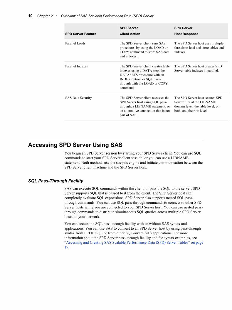
Parallel Loads The SPD Server client runs SAS procedures by using the LOAD or COPY command to store SAS data and indexes.
The SPD Server host uses multiple threads to load and store tables and indexes.
Parallel Indexes The SPD Server client creates table indexes using a DATA step, the DATASETS procedure with an INDEX option, or SQL pass-through with the LOAD or COPY command.
The SPD Server host creates SPD Server table indexes in parallel.
SAS Data Security The SPD Server client accesses the SPD Server host using SQL pass-through, a LIBNAME statement, or an alternative connection that is not part of SAS.
The SPD Server host secures SPD Server files at the LIBNAME domain level, the table level, or both, and the row level.
Accessing SPD Server Using SASYou begin an SPD Server session by starting your SPD Server client. You can use SQL commands to start your SPD Server client session, or you can use a LIBNAME statement. Both methods use the sasspds engine and initiate communication between the SPD Server client machine and the SPD Server host.
SQL Pass-Through FacilitySAS can execute SQL commands within the client, or pass the SQL to the server. SPD Server supports SQL that is passed to it from the client. The SPD Server host can completely evaluate SQL expressions. SPD Server also supports nested SQL pass-through commands. You can use SQL pass-through commands to connect to other SPD Server hosts while you are connected to your SPD Server host. You can use nested pass-through commands to distribute simultaneous SQL queries across multiple SPD Server hosts on your network.
You can access the SQL pass-through facility with or without SAS syntax and applications. You can use SAS to connect to an SPD Server host by using pass-through syntax from PROC SQL or from other SQL-aware SAS applications. For more information about the SPD Server pass-through facility and for syntax examples, see “Accessing and Creating SAS Scalable Performance Data (SPD) Server Tables” on page 19.
10 Chapter 2 • Overview of SAS Scalable Performance Data (SPD) Server

Securing SAS Data
Registering the LIBNAME DomainSPD Server data resides in domains. A domain is similar in structure to a directory. Your SPD Server administrator will configure your SPD Server domains when your userID is created.
ACL File SecuritySPD Server uses access control lists (ACLs) and SPD Server user IDs to secure domain resources. You obtain your user ID and password from your SPD Server administrator.
SPD Server supports ACL groups, which are similar to UNIX groups. SPD Server administrators can associate an SPD Server user with as many as thirty-two different ACL groups.
ACL file security is turned on by default when an administrator starts an SPD Server. ACL permissions affect all SPD Server resources, including domains, tables, table columns, catalogs, catalog entries, and utility files. When ACL file security is enabled, SPD Server grants access rights only to the owner (creator) of an SPD Server resource. Resource owners can use PROC SPDO to grant ACL permissions to a specific group (ACL group) or to all SPD Server users.
The resource owner can use the following properties to grant ACL permissions to all SPD Server users:
READuniversal Read access to the resource (read or query)
WRITEuniversal Write access to the resource (append to or update)
ALTERuniversal Alter access to the resource (rename, delete, or replace a resource, and add or delete indexes associated with a table)
The resource owner can use the following properties to grant ACL permissions to a named ACL group:
GROUPREADgroup Read access to the resource (read or query)
GROUPWRITEgroup Write access to the resource (append to or update)
GROUPALTERgroup Alter access to the resource (rename, delete, or replace a resource, and add or delete indexes associated with a table)
Securing SAS Data 11

SPD Server Extensions to Base SASYou can access SPD Server by using an SQL pass-through CONNECT statement, or you can issue a SAS LIBNAME statement. After you connect to SPD Server, you can run SAS DATA steps, SAS procedures, or PROC SQL statements.
This document and the SPD Server Administrator's Guide provide syntax and examples that use SPD Server extensions to Base SAS language. Most of your existing SAS programs will function in SPD Server with only minor modifications.
SPD Server uses the following extensions to the Base SAS language:
• LIBNAME statement options
• SPD Server SQL pass-through syntax
• table options
• macro variables
• parallel WHERE clause processing
• parallel GROUP BY processing
• BY data grouping
• parallel index creation
• the operator interface procedure PROC SPDO
12 Chapter 2 • Overview of SAS Scalable Performance Data (SPD) Server

Chapter 3
Connecting to SAS Scalable Performance Data (SPD) Server
Introduction . . . . . . . . . . . . . . . . . . . . . . . . . . . . . . . . . . . . . . . . . . . . . . . . . . . . . . . . . . 13
Accessing SPD Server from a SAS Client . . . . . . . . . . . . . . . . . . . . . . . . . . . . . . . . . . 13SQL Pass-Through Facility . . . . . . . . . . . . . . . . . . . . . . . . . . . . . . . . . . . . . . . . . . . 13LIBNAME Access . . . . . . . . . . . . . . . . . . . . . . . . . . . . . . . . . . . . . . . . . . . . . . . . . . 14LIBNAME Options . . . . . . . . . . . . . . . . . . . . . . . . . . . . . . . . . . . . . . . . . . . . . . . . . 15Connect to a Specified SPD Server Host . . . . . . . . . . . . . . . . . . . . . . . . . . . . . . . . . 15Manage Server Network Traffic . . . . . . . . . . . . . . . . . . . . . . . . . . . . . . . . . . . . . . . . 17Additional LIBNAME Options . . . . . . . . . . . . . . . . . . . . . . . . . . . . . . . . . . . . . . . . 17Examples of the LIBNAME Statement . . . . . . . . . . . . . . . . . . . . . . . . . . . . . . . . . . 18
SPD Server Table Options . . . . . . . . . . . . . . . . . . . . . . . . . . . . . . . . . . . . . . . . . . . . . . 18
IntroductionThis chapter describes how to access SPD Server by using SAS and the SPD Server SQL pass-through facility, or by using a SAS LIBNAME statement. The chapter demonstrates typical data tasks on an SPD Server host. Power users who have special privileges should see Chapter 21, “SAS Scalable Performance Data (SPD) Server Operator Interface Procedure (PROC SPDO) ,” in SAS Scalable Performance Data Server: Administrator's Guide.
Note: For readability, this chapter refers to the SPD Server SQL pass-through facility as simply the SQL pass-through facility, unless the context requires a more explicit reference. Similarly, when the chapter references a name server, it is the SPD Server name server.
Accessing SPD Server from a SAS Client
SQL Pass-Through FacilityTo connect to an SPD Server SQL server from a SAS session, you must submit a CONNECT statement that specifies the SASSPDS engine and SPD Server options and then issues the SQL commands.
For example:
13

PROC SQL; connect to sasspds (dbq='mydomain' host='namesvrID' serv='5555' user='neraksr' passwd='siuya'); select * from connection to sasspds (select * from employee_info); disconnect from sasspds; quit;
LIBNAME Access
Overview of LIBNAME AccessA logical name or libref is a name for the data library that you associate with an SPD Server domain during a SAS job or session. After a libref is assigned, SPD Server enables you to read, create, or update files in the data library if you have the appropriate access to the data library.
A libref is valid only for the current SAS job or session. Librefs can be referenced repeatedly during a valid job or session. SAS does not limit the number of librefs that you can assign during a session. After you define a libref, it is most commonly used as the first element in two-level SAS filenames: LibraryName.Tablename. The library name or libref identifies where the SPD Server can find or store the file.
LIBNAME libref SASSPDS <'SAS-data-library'> <SPD Server-options>;
Use the following arguments:
librefa name up to 8 characters long that conforms to the rules for SAS names.
SASSPDSthe name of the SPD Server engine.
'SAS-data-library'the logical LIBNAME domain name for an SPD Server data library on the host machine. The name server resolves the domain name into the physical path for the library.
SPD Server-optionsone or more SPD Server options.
The section, “Using a LIBNAME Statement to Access SPD Server” on page 21contains examples of LIBNAME connections to SPD Server.
Example Using a Libref with LIBNAME AccessThe following statement creates the table TRAVEL and stores it in a permanent SAS library with the libref ANNUAL:
data annual.travel;
The following is a LIBNAME statement that associates a libref, the SASSPDS engine, and an SPD Server domain:
LIBNAME mydatalib sasspds 'mydomain'
14 Chapter 3 • Connecting to SAS Scalable Performance Data (SPD) Server

host='namesvrID' serv='5555' user='neraksr' passwd='siuya';
LIBNAME OptionsYou must supply the SASSPDS engine name to access SPD Server LIBNAME domains with a LIBNAME statement. You must specify one or more SPD Server options. Here is the syntax for an SPD Server option:
<SPD Server-option>=<value>;
SPD Server-optiona keyword to name the option
valuea value expected by the keyword
Option values in a LIBNAME statement enable the engine to initiate, manage, and customize a client session.
Connect to a Specified SPD Server Host
Overview of Connecting to a Specified SPD Server HostTo connect to a host, SPD Server needs the network node name for the SPD Server host machine or the IP address of the server machine, and the port number of a name server. SPD Server provides the following options to locate a name server using a named service:
SERVER=specifies a node name for an SPD Server host machine and a port number for the name server that is running on the machine.
HOST=specifies a node for an SPD Server host machine and a port number for the name server that is running on the machine.
Both options have the same function. SERVER= arguments are compatible with SAS/SHARE software. HOST= arguments support FTP conventions. You can use the HOST option to specify an IP address (for example, 123.456.76.1) for the node. The SERVER option requires a network node name.
SPDSHOST= Macro VariableIf you create a SAS macro variable named SPDSHOST= or an environment variable named SPDSHOST=, then whenever a LIBNAME statement does not specify an SPD Server host machine, SPD Server looks for the value of SPDSHOST= to identify the host server.
%let spdshost=samson; LIBNAME myref sasspds 'mylib' user='yourid' password='swami';
Accessing SPD Server from a SAS Client 15
The first statement assigns the SPD Server host SAMSON to the macro variable SPDSHOST. Therefore, a subsequent LIBNAME statement does not need to name the host server again.
Validating the Client User IDSPD Server uses ACL file security to secure domain resources. If ACL file security is enabled, the SPD Server grants access in the following order:
1. uses the permissions that belong to the UNIX ID that is associated with the SPD Server
2. uses the permissions that belong to the SPD Server user ID
You can use SQL pass-through and LIBNAME statement options to specify the identity of an SPD Server user. SPD Server uses a special ID table to validate user IDs and passwords. The following LIBNAME options identify a client:
ACLGRP=specifies one to five ACL groups that the user can belong to.
ACLSPECIAL=grants special privileges to an SPD Server user who was previously set up as special. (ACLSPECIAL=YES is defined for the user in the password file.) Special privileges override other ACL restrictions that apply to resources in the domain.
CHNGPASS=prompts a client user to change his or her SPD Server password.
NEWPASSWORD= or NEWPASSWD=specifies a new password for an SPD Server client user.
PASSWORD= or PASSWD=specifies a password to validate an SPD Server client user.
PROMPT=prompts for a password to validate an SPD Server client user.
PASSTHRU=specifies implicit SQL pass-through options for an SPD Server client user.
USER=specifies the SPD Server user ID.
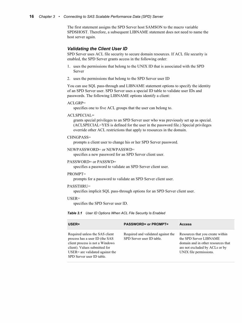
Table 3.1 User ID Options When ACL File Security Is Enabled
USER= PASSWORD= or PROMPT= Access
Required unless the SAS client process has a user ID (the SAS client process is not a Windows client). Values submitted for USER= are validated against the SPD Server user ID table.
Required and validated against the SPD Server user ID table.
Resources that you create within the SPD Server LIBNAME domain and in other resources that are not excluded by ACLs or by UNIX file permissions.
16 Chapter 3 • Connecting to SAS Scalable Performance Data (SPD) Server
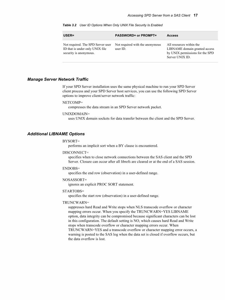
Table 3.2 User ID Options When Only UNIX File Security Is Enabled
USER= PASSWORD= or PROMPT= Access
Not required. The SPD Server user ID that is under only UNIX file security is anonymous.
Not required with the anonymous user ID.
All resources within the LIBNAME domain granted access by UNIX permissions for the SPD Server UNIX ID.
Manage Server Network TrafficIf your SPD Server installation uses the same physical machine to run your SPD Server client process and your SPD Server host services, you can use the following SPD Server options to improve client/server network traffic:
NETCOMP=compresses the data stream in an SPD Server network packet.
UNIXDOMAIN=uses UNIX domain sockets for data transfer between the client and the SPD Server.
Additional LIBNAME OptionsBYSORT=
performs an implicit sort when a BY clause is encountered.
DISCONNECT=specifies when to close network connections between the SAS client and the SPD Server. Closure can occur after all librefs are cleared or at the end of a SAS session.
ENDOBS=specifies the end row (observation) in a user-defined range.
NOSASSORT=ignores an explicit PROC SORT statement.
STARTOBS=specifies the start row (observation) in a user-defined range.
TRUNCWARN=suppresses hard Read and Write stops when NLS transcode overflow or character mapping errors occur. When you specify the TRUNCWARN=YES LIBNAME option, data integrity can be compromised because significant characters can be lost in this configuration. The default setting is NO, which causes hard Read and Write stops when transcode overflow or character mapping errors occur. When TRUNCWARN=YES and a transcode overflow or character mapping error occurs, a warning is posted to the SAS log when the data set is closed if overflow occurs, but the data overflow is lost.
Accessing SPD Server from a SAS Client 17
Examples of the LIBNAME Statement
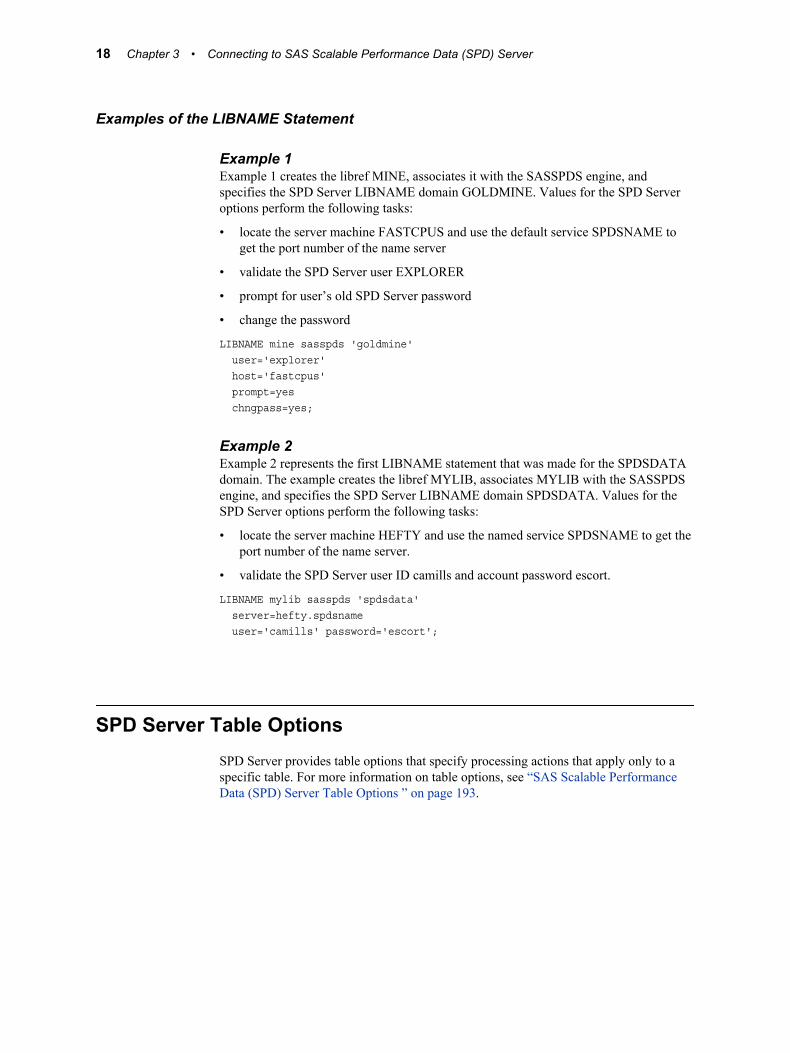
Example 1Example 1 creates the libref MINE, associates it with the SASSPDS engine, and specifies the SPD Server LIBNAME domain GOLDMINE. Values for the SPD Server options perform the following tasks:
• locate the server machine FASTCPUS and use the default service SPDSNAME to get the port number of the name server
• validate the SPD Server user EXPLORER
• prompt for user’s old SPD Server password
• change the password
LIBNAME mine sasspds 'goldmine' user='explorer' host='fastcpus' prompt=yes chngpass=yes;
Example 2Example 2 represents the first LIBNAME statement that was made for the SPDSDATA domain. The example creates the libref MYLIB, associates MYLIB with the SASSPDS engine, and specifies the SPD Server LIBNAME domain SPDSDATA. Values for the SPD Server options perform the following tasks:
• locate the server machine HEFTY and use the named service SPDSNAME to get the port number of the name server.
• validate the SPD Server user ID camills and account password escort.
LIBNAME mylib sasspds 'spdsdata' server=hefty.spdsname user='camills' password='escort';
SPD Server Table OptionsSPD Server provides table options that specify processing actions that apply only to a specific table. For more information on table options, see “SAS Scalable Performance Data (SPD) Server Table Options ” on page 193.
18 Chapter 3 • Connecting to SAS Scalable Performance Data (SPD) Server

Chapter 4
Accessing and Creating SAS Scalable Performance Data (SPD) Server Tables
SAS and SPD Server Tables . . . . . . . . . . . . . . . . . . . . . . . . . . . . . . . . . . . . . . . . . . . . 19Overview of SPD Server Tables . . . . . . . . . . . . . . . . . . . . . . . . . . . . . . . . . . . . . . . . 19SAS Libraries . . . . . . . . . . . . . . . . . . . . . . . . . . . . . . . . . . . . . . . . . . . . . . . . . . . . . . 20Temporary LIBNAME Domains . . . . . . . . . . . . . . . . . . . . . . . . . . . . . . . . . . . . . . . 20
SPD Server Resource Security . . . . . . . . . . . . . . . . . . . . . . . . . . . . . . . . . . . . . . . . . . 20UNIX File Security . . . . . . . . . . . . . . . . . . . . . . . . . . . . . . . . . . . . . . . . . . . . . . . . . . 20ACL File Security . . . . . . . . . . . . . . . . . . . . . . . . . . . . . . . . . . . . . . . . . . . . . . . . . . . 21
Using a LIBNAME Statement to Access SPD Server . . . . . . . . . . . . . . . . . . . . . . . . 21Overview of Using a LIBNAME Statement . . . . . . . . . . . . . . . . . . . . . . . . . . . . . . . 21Issuing an Initial LIBNAME Statement . . . . . . . . . . . . . . . . . . . . . . . . . . . . . . . . . . 22
Managing Large SPD Server Files . . . . . . . . . . . . . . . . . . . . . . . . . . . . . . . . . . . . . . . 22
Migrating Tables between SAS and SPD Server . . . . . . . . . . . . . . . . . . . . . . . . . . . . 22SAS and SPD Server Table Migration Examples . . . . . . . . . . . . . . . . . . . . . . . . . . . 22
Accessing and Manipulating Data with the SQL Pass-Through Facility . . . . . . . . 24Overview of the SQL Pass-Through Facility . . . . . . . . . . . . . . . . . . . . . . . . . . . . . . 24Accessing Data Using the SQL Pass-Through Facility . . . . . . . . . . . . . . . . . . . . . . 24SQL Pass-Through Statements . . . . . . . . . . . . . . . . . . . . . . . . . . . . . . . . . . . . . . . . . 24Examples of Using the SQL Pass-Through Facility . . . . . . . . . . . . . . . . . . . . . . . . . 27
Creating a New Table . . . . . . . . . . . . . . . . . . . . . . . . . . . . . . . . . . . . . . . . . . . . . . . . . . 28Creating a New Table Using Pass-Through Statements . . . . . . . . . . . . . . . . . . . . . . 28Creating a New Table with a LIBNAME Statement . . . . . . . . . . . . . . . . . . . . . . . . 29
SAS and SPD Server Tables
Overview of SPD Server TablesSPD Server tables have different physical structures than SAS tables. In a general discussion, a SAS table can also refer to an SPD Server table. If the context is specific (for example, an SPD Server command), then the reference is specific. A SAS table refers to the Base SAS format. An SPD Server table refers to the SPD Server format.
Using SPD Server and SAS together, you can accomplish the following tasks:
• convert tables from the Base SAS format to the SPD Server format
• convert tables from the SPD Server format to the Base SAS format
19

• create a new SPD Server table
• read, query, append to, update, sort, and index SPD Server tables
SAS LibrariesThe term SAS library refers to a collection of SAS files or a collection of SPD Server files. For SPD Server, a SAS library or data library is a collection of one or more directories that specifies the location of stored SPD Server files. A data library has a primary file system. The primary file system is the directory an SPD Server administrator defines for the LIBNAME domain when it is set up. In addition, a SAS library can have other directories for separating SPD Server component files.
An SPD Server data library can contain the following LIBNAME domain files:
• SPD Server tables
• SPD Server indexes
• SPD Server catalogs
• SPD Server ACL files
• SPD Server utility files, such as a VIEW, multidimensional database (MDDB), and so on
Temporary LIBNAME DomainsSPD Server enables you to create temporary LIBNAME domains that exist only for the duration of the LIBNAME assignment. SPD Server users can create space analogous to the SAS Work library. To create a temporary LIBNAME domain, use the SPD Server LIBNAME statement option, TEMP=YES.
When you end your SPD Server session, all of the data objects, including tables, catalogs, and utility files in the TEMP=YES temporary domain are automatically deleted. The SAS Work library functions similarly.
SPD Server Resource SecuritySPD Server provides two levels of data security: UNIX file security and ACL file security. ACL file security enforces SPD Server permissions with SPD Server user IDs and ACLs.
UNIX File SecuritySPD Server enables ACL file security by default. Although you should use ACL file security, an SPD Server administrator can change the default ACL file security setting. When an SPD Server administrator specifies the NOACL option, all clients of SPD Server obtain the SPD Server user ID anonymous. No SPD Server security is in effect. SPD Server tables are secured only by the UNIX file protections that are currently in place.
When UNIX file security controls SPD Server file access, it validates on the user ID associated with SPD Server. The UNIX ID associated with SPD Server is the UNIX ID of the user that starts the server. Suppose an SPD Server administrator starts the SPD Server host machine, using his SPD Server administrator's account named SPDSADMN.
20 Chapter 4 • Accessing and Creating SAS Scalable Performance Data (SPD) Server Tables
When any SAS client connects to this SPD Server host, the client can read only files that have UNIX Read permissions set for the SPDSADMN user. As a result, SAS clients that are connected to this SPD Server host must write all files in a directory created by SPDSADMIN that also has Write permission set for SPDSADMN. SPDSADMN owns all files written in this directory.
Security is maintained as a result of the SPD Server administrator setting up SPD Server LIBNAME domain directories so that only he has Read and Write access to those directories.
It is possible for a site to give different UNIX permissions to a group of users. An SPD Server administrator must start another SPD Server using a different UNIX user account. (Starting a different SPD Server affects only new SPD Server files, not existing SPD Server files.)
ACL File SecurityUNIX file security alone is not adequate for many installations. For more complex workplace environments, SPD Server provides a finer level of control called ACL file security. ACL file security is used by default for SPD Server LIBNAME domains. SPD Server always enforces ACL file security unless an SPD Server administrator specifies the NOACL option when starting the server.
To understand ACL file security, you must know how SPD Server user IDs work. The SPD Server administrator assigns each approved SPD Server user an ID, a password, a level of data authorization, and membership (optional) in up to five ACL groups. (The SPD Server user ID anonymous does not require a password.)
After the SPD Server administrator creates your SPD Server user ID, you and the SPD Server administrator can use PROC SPDO to create ACLs that grant or deny other users access to an SPD Server table.
Using a LIBNAME Statement to Access SPD Server
Overview of Using a LIBNAME StatementYou do not need to understand all possible LIBNAME and table options to initiate an SPD Server client session. The LIBNAME statement should specify the following items:
• the local library reference (libref)
• the required engine name (SASSPDS)
• a valid domain name that is registered to the name server and defined to the SPD Server host
• the name of the name server’s host
• the user ID
• password access, either using the PROMPT=YES switch or using the PASSWD keyword. (Using the PROMPT=YES switch is the more secure method.)
Using a LIBNAME Statement to Access SPD Server 21

Issuing an Initial LIBNAME StatementThe following example specifies the libref market, the engine name sasspds, the LIBNAME domain mktdata, and the name server host sunone. It identifies an SPD Server user ID and is configured to prompt the user for a password.
LIBNAME market sasspds 'mktdata' host='sunone' user='user id' prompt=yes;
Instead of using the previous code to access SPD Server, you could use the following:
LIBNAME market sasspds 'mktdata' host='sunone' user='user id' passwd='beemer';
The only difference between this example and the previous example is the password specification. In the second example, the password beemer is included in the LIBNAME statement. You can use this method for batched SPD Server jobs that run unattended.
Managing Large SPD Server FilesManaging large files is not only a performance issue; it also has implications for file storage and disk space. Optimally, an SPD Server administrator manages storage space for SPD Server LIBNAME domains. In that case, you do not need to consider storage issues. SPD Server does the work for you.
Migrating Tables between SAS and SPD Server
SAS and SPD Server Table Migration Examples
Create a SAS Table from an SPD Server TableTo create a SAS table from an SPD Server table, issue a LIBNAME statement, but do not specify the engine SASSPDS. Your program creates a Base SAS table. (Later, if you decide to use SPD Server capabilities, you can convert the Base SAS table to the SPD Server format. Conversion is easy. Interchange table formats using the COPY procedure. See “Convert from SAS to SPD Server Format” on page 23.)
/* Create local racquets data set. */ LIBNAME local '/u/sasdemo/local';
data local.racquets; input racquet_name $20. @22 weight_oz @28 balance $2. @32 flex @36 gripsize @42 string_type $3. @47 retail_price @55 inventory_onhand;
22 Chapter 4 • Accessing and Creating SAS Scalable Performance Data (SPD) Server Tables
datalines; Filbert VolleyMaster 10.5 HL 5 4.5 syn 129.95 5 Solo Queensize 10.9 HH 6 5.0 syn 130.00 3 Perkinson AllCourt 11.0 N 5 4.25 syn 159.99 12 Wilco Specialist 8.9 HL 3 5.0 nat 287.50 1 ;
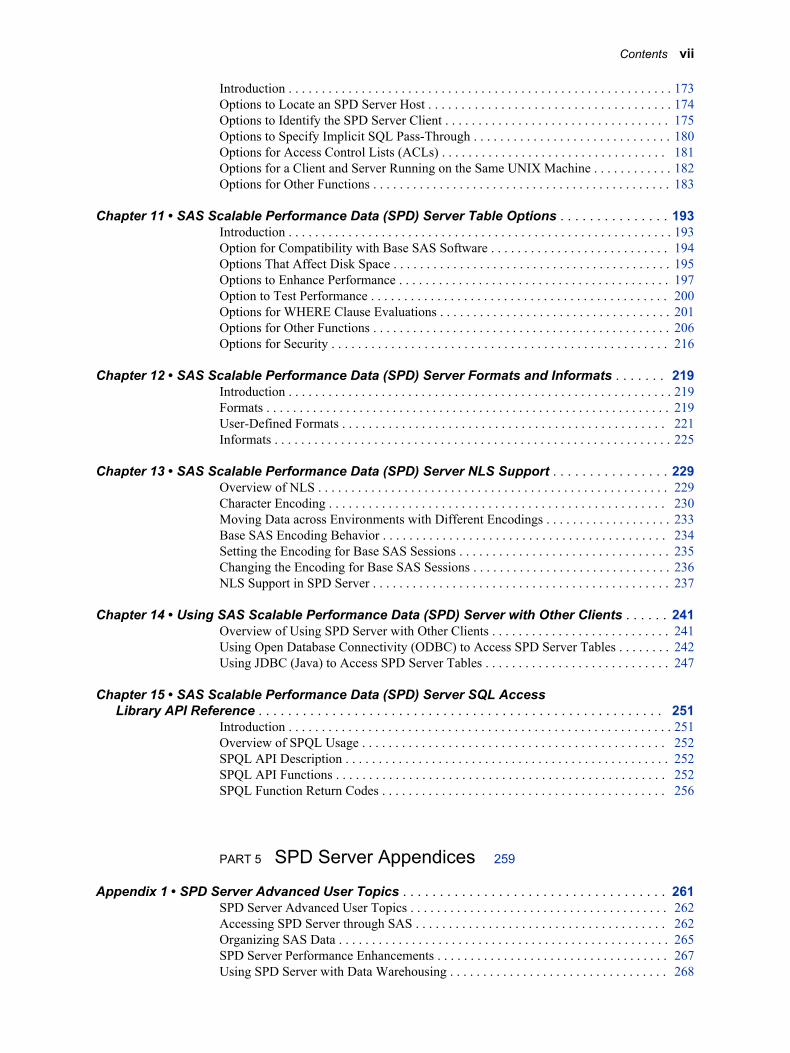
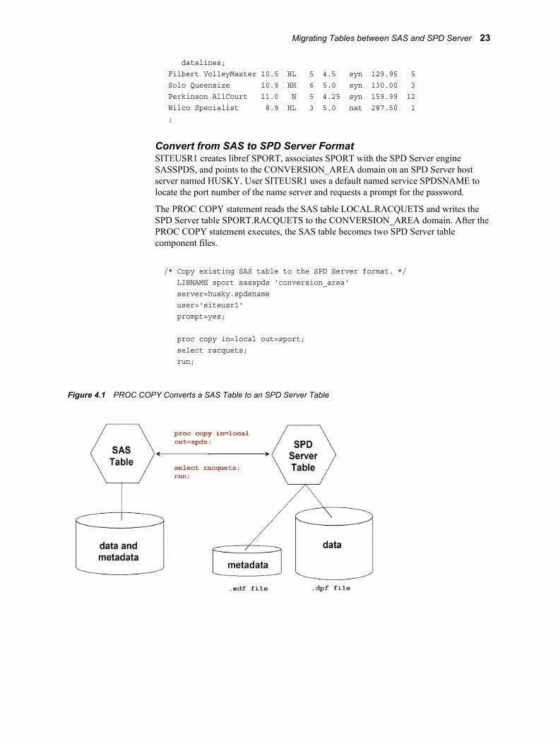
Convert from SAS to SPD Server FormatSITEUSR1 creates libref SPORT, associates SPORT with the SPD Server engine SASSPDS, and points to the CONVERSION_AREA domain on an SPD Server host server named HUSKY. User SITEUSR1 uses a default named service SPDSNAME to locate the port number of the name server and requests a prompt for the password.
The PROC COPY statement reads the SAS table LOCAL.RACQUETS and writes the SPD Server table SPORT.RACQUETS to the CONVERSION_AREA domain. After the PROC COPY statement executes, the SAS table becomes two SPD Server table component files.
/* Copy existing SAS table to the SPD Server format. */ LIBNAME sport sasspds 'conversion_area' server=husky.spdsname user='siteusr1' prompt=yes;
proc copy in=local out=sport; select racquets; run;
Figure 4.1 PROC COPY Converts a SAS Table to an SPD Server Table
Migrating Tables between SAS and SPD Server 23
Accessing and Manipulating Data with the SQL Pass-Through Facility
Overview of the SQL Pass-Through FacilitySPD Server uses SQL pass-through commands to access and manipulate data. The SQL pass-through facility provides SPD Server clients with an alternative way to establish a connection with an SPD Server host or to directly load from an external database such as Oracle. Users have access in the SPD Server environment and increased connectivity to external databases using the SPD Server engine.
For reference information about SQL syntax in SPD Server, see “ SAS Scalable Performance Data (SPD) Server SQL Syntax Reference Guide” on page 306.
Accessing Data Using the SQL Pass-Through FacilityThe SQL pass-through facility is an access method that allows SPD Server to connect to an SQL server and manipulate data. To use SQL pass-through, do the following tasks:
1. Establish a connection from an SPD Server client using a CONNECT statement.
2. Send SPD Server SQL statements using the EXECUTE statement.
3. Retrieve data with the CONNECTION TO component in a SELECT statement's FROM clause.
4. Terminate the connection using the DISCONNECT statement.
For examples of how to do these tasks, see “Examples of Using the SQL Pass-Through Facility” on page 27.
SQL Pass-Through Statements
CONNECT StatementThe CONNECT statement specifies the SAS I/O engine that provides SQL pass-through access.
Syntax
CONNECT TO dbms-name<AS alias>(dbms-args);
Arguments:
dbms-name (required)specifies the name of the engine.
When you are running SAS and PROC SQL, you must specify sasspds to obtain SQL pass-through to an SPD Server SQL server. You must specify spdseng to obtain SQL pass-through from an SPD Server SQL server.
Note: spdseng is the database you use to reference an SPD Server from within an existing SPD Server SQL connection.
24 Chapter 4 • Accessing and Creating SAS Scalable Performance Data (SPD) Server Tables

AS alias (optional)specifies an alias or logical name for a connection. When you specify an alias to identify the connection, use a string that is not enclosed in quotation marks. Refer to this logical name in subsequent SQL pass-through statements.
Note: For the alias, you must specify the connection that executes the statement.
The following two examples show how to use an alias:
execute(...) by alias
select * from connection to alias(...)
dbms-args (required and optional arguments)identifies the SQL server and the data source. The following dbms-args arguments are for the SPD Server engines, sasspds and spdseng. SPD Server SQL uses the syntax keyword=value.
DBQ=libname-domain (required)specifies the primary SPD Server LIBNAME domain for the SQL pass-through connection. The name that you specify must be identical to the LIBNAME domain name that you used when you assigned a SAS LIBNAME to sasspds. Enclose the value in single or double quotation marks.
HOST=name-server-host (optional)specifies a node name or an IP address for a name server that is currently running. Enclose the string in single or double quotation marks. If you do not specify a value, SPD Server uses the current value of the SAS macro variable spdshost to determine the node name.
SERVICE=name-server-port (optional)SERV=name-server-port (optional)
specifies the network address (port number) for a name server that is currently running. Enclose the value in single or double quotation marks. If you do not specify a port number for the name server, SPD Server determines the network address from the named service spdsname in the/etc/services file.
USER=SPD Server user ID (required on Windows, but not on UNIX)specifies an SPD Server user ID to access an SPD Server SQL server. Enclose the value in single or double quotation marks.
Note: On UNIX, it is not necessary to specify USER= on a CONNECT statement because SPD Server assumes the UNIX userID.
PASSWORD=password (required, or use PROMPT=YES unless USER='anonymous')PASSWD=password (required, or use PROMPT=YES unless USER='anonymous')
specifies an SPD Server user ID password to access an SPD Server. This value is case sensitive. You should not specify a password in a text file that another user can view. You should use this argument in a batch job that is protected by file- system permissions, which prohibits other users from reading the text file.
PROMPT=YES (required, or use PASSWD= or PASSWORD= unless USER='anonymous')
specifies a password prompt to access an SPD Server SQL server. This value is case sensitive.
DISCONNECT StatementThe DISCONNECT statement disconnects you from your database management system (DBMS) source. When you no longer need the PROC SQL connection, you must disconnect from the DBMS source. You are automatically disconnected when you exit
Accessing and Manipulating Data with the SQL Pass-Through Facility 25

PROC SQL. However, you can explicitly disconnect from the DBMS source by using the DISCONNECT statement.
Syntax
DISCONNECT FROM [dbms-name | alias];
Arguments
dbms-namethe name specified in the CONNECT statement that established the connection.
aliasthe alias value specified in the CONNECT statement that established the connection.
EXECUTE StatementThe EXECUTE statement is part of the SQL pass-through facility. Use this statement to use specific SQL statements that do not return a results set during a pass-through connection. Before you use the EXECUTE statement, you must establish a connection by using the CONNECT statement. After you create a pass-through connection, use the EXECUTE statement to submit valid SQL statements (you cannot submit the SELECT statement).
Syntax
EXECUTE (SQL-statement) BY [dbms-name | alias];
Arguments
(SQL-statement)a valid SQL statement that is passed for execution (you cannot specify the SELECT statement because it attempts to return query results). This argument is required and must be enclosed within parentheses.
dbms-name (required, or use alias)identifies the DBMS to which you want to direct the SQL statement. The dbms-name value must be preceded by the keyword BY. You must specify either the dbms-name, or the alias in your CONNECT statement.
alias (required if you did not provide dbms-name)specifies an alias that is used in the CONNECT statement. If you do not specify the dbms-name, in your CONNECT statement, then you must specify the alias.
CONNECTION TO StatementCONNECTION TO is an SQL pass-through component that you can use in the FROM clause of a SELECT statement as part of the from list. The CONNECTION TO component enables you to make pass-through queries for data and to use that data in a PROC SQL query or table. PROC SQL treats the results of the query like a virtual table.
Syntax
CONNECTION TO [dbms-name | alias](SQL-query)
;
Arguments
dbms-name (required)If you have a single connection, dbms-name is the same dbms-name value that you specified in your CONNECT statement. If you have multiple connections, use the alias that you specified in the AS clause of the CONNECT statement. If you do not specify dbms-name in your CONNNECTION TO statement, you must specify the alias that was established in the CONNECT statement.
26 Chapter 4 • Accessing and Creating SAS Scalable Performance Data (SPD) Server Tables

(SQL-query)specifies the SQL query that you want to send. Your SQL query cannot contain a semicolon because a semicolon represents the end of a statement to SPD Server. Character literals are limited to 32,000 characters. Make sure that your SQL query is enclosed in parentheses.
alias (required if you did not provide dbms-name)specifies the alias that was used in the CONNECT statement. If you do not specify the dbms-name value, then you must specify the alias value.
alias (optional)specifies the optional alias that you used in the CONNECT statement.
Examples of Using the SQL Pass-Through Facility
Using PROC SQL to Connect to a SQL ServerIn this example, we issue a CONNECT statement to connect from a SAS session to an SPD Server SQL server. After the connection is made, the first EXECUTE statement creates a table named EMPLOYEE_INFO with three columns:EMPLOYEE_NO, EMPLOYEE_NAME, and ANNUAL_SALARY. The second EXECUTE statement inserts an observation into the table where EMPLOYEE_NO equals 1, EMPLOYEE_NAME equals The Prez, and ANNUAL_SALARY equals 10,000.
The subsequent FROM CONNECTION TO statement retrieves all of the records from the new EMPLOYEE_INFO table. (In this example, it retrieves a single observation, which was inserted by the second EXECUTE statement.) The DISCONNECT statement terminates the connection.
PROC SQL; connect to sasspds (dbq='mydomain' host='workstation1' serv='spdsname' user='me' passwd='noway');
execute (create table employee_info (employee_no num, employee_name char(30), annual_salary num)) by sasspds;
execute (insert into employee_info values (1, 'The Prez', 10000)) by sasspds;
select * from connection to sasspds (select * from employee_info); disconnect from sasspds; quit;
Nesting SQL Pass-Through AccessYou can nest SPD Server pass-through access. Nesting allows access to data that is stored on two different networks or network nodes. You can use the spdseng database to reserve an SPD Server from within an existing SPD Server SQL connection.
Accessing and Manipulating Data with the SQL Pass-Through Facility 27

In the following example, on the DATAGATE host on a local network, SQL pass-through is nested to access the EMPLOYEE_INFO table. This table is available on the PROD host on a remote network. (You must have user access to the PROD host.)
proc sql; connect to sasspds (dbq='domain1' host='datagate' serv='spdsname' user='usr1' passwd='usr1_pw'); execute (connect to spdseng (dbq='domain2' host='prod' serv='spdsname' user='usr2' passwd='usr2_pw')) by sasspds; select * from connection to sasspds( select * from connection to spdseng( select employee_no, annual_salary from employee_info)); execute (disconnect from spdseng) by sasspds; disconnect from sasspds; quit;
Note: If you would prefer not to use the spdseng database to reference a server, you can use the LIBGEN=YES option. Libraries with the LIBGEN=YES option are automatically available in SQL environments. For more information about the LIBGEN=YES option, see “LIBGEN=” on page 187
Creating a New Table
Creating a New Table Using Pass-Through StatementsIn this example, we connect from a SAS session to an SPD Server SQL server and execute a CONNECT statement. After making the connection, the first EXECUTE statement creates a table named LOTTERYWIN with two columns: TICKETNO and WINNAME. The second EXECUTE statement inserts an observation into the table where TICKETNO equals 1 and NAME equals Wishu Weremee.
The subsequent FROM CONNECTION TO statement retrieves all of the records from the new LOTTERYWIN table. (In this example, it retrieves a single observation, which was inserted by the second EXECUTE statement. The DISCONNECT statement terminates the connection.
proc sql; connect to sasspds (dbq='mydomain' host='workstation1' serv='spdsname' user='me' passwd='luckyones'); execute (create table lotterywin (ticketno num, winname char(30))) by sasspds; execute (insert into lotterywin values (1, 'Wishu Weremee')) by sasspds; select * from connection to sasspds (select * from employee); disconnect from sasspds; quit;
28 Chapter 4 • Accessing and Creating SAS Scalable Performance Data (SPD) Server Tables
Creating a New Table with a LIBNAME StatementThis example illustrates how SITEUSR1 creates a new SPD Server table named CARDATA.OLD_AUTOS on the server.
LIBNAME cardata sasspds 'conversion_area' server=husky.5105 user='siteusr1' prompt=yes;
/* Create the table CARDATA.OLD_AUTOS on the SPD Server host. */
data cardata.old_autos; input year $4. @6 manufacturer $12. model $12. body_style $5. engine_liters @39 transmission_type $1. @41 exterior_color $10. options $10. mileage conditon;
datalines;
1966 Ford Mustang conv 3.5 M white 00000001 143000 21967 Chevrolet Corvair sedan 2.2 M burgundy 00000001 70000 31975 Volkswagen Beetle 2door 1.8 M yellow 00000010 80000 41987 BMW 325is 2door 2.5 A black 11000010 110000 31962 Nash Metropolitan conv 1.3 M red 00000111 125000 3;
Creating a New Table 29

30 Chapter 4 • Accessing and Creating SAS Scalable Performance Data (SPD) Server Tables

Chapter 5
Indexing, Sorting, and Manipulating SAS Scalable Performance Data (SPD) Server Tables
Indexing Tables . . . . . . . . . . . . . . . . . . . . . . . . . . . . . . . . . . . . . . . . . . . . . . . . . . . . . . . 31Overview of Indexing Tables . . . . . . . . . . . . . . . . . . . . . . . . . . . . . . . . . . . . . . . . . . 31
Examples of Creating SPD Server Indexes . . . . . . . . . . . . . . . . . . . . . . . . . . . . . . . . 31Example 1: Creating SPD Server Indexes from a DATA Step . . . . . . . . . . . . . . . . 31Example 2: Creating SPD Server Indexes from PROC DATASETS . . . . . . . . . . . 32Example 3: Creating SPD Server Indexes By Using SQL . . . . . . . . . . . . . . . . . . . . 32Example 4: Creating SPD Server Indexes Using Pass-Through SQL . . . . . . . . . . . 32Example 5: Using VERBOSE= to See Index Information . . . . . . . . . . . . . . . . . . . . 32Example 6: Using PROC SORT with SPD Server . . . . . . . . . . . . . . . . . . . . . . . . . . 33Example 7: Using the Implicit SPD Server BY Clause Sort . . . . . . . . . . . . . . . . . . 33Example 8: Using PROC SORT . . . . . . . . . . . . . . . . . . . . . . . . . . . . . . . . . . . . . . . . 33
Indexing Tables
Overview of Indexing TablesSPD Server efficiently indexes tables of varying size and data distributions. The SPD Server SPD index supports queries that require global table views (such as queries that contain BY clause processing or SQL joins), or queries that require segmented views (such as parallel processing of WHERE clause statements).
Examples of Creating SPD Server Indexes
Example 1: Creating SPD Server Indexes from a DATA StepThe following code creates SPD Server table X. Next, the code creates a simple SPD Server index X on column X, and a composite SPD Server index Y on columns (A B).
data foo.x( index=(x y=(a b))); x=1; a="Doe"; b=20; run;
31

Example 2: Creating SPD Server Indexes from PROC DATASETSThe following code creates the same simple and composite SPD Server indexes that were created in Example 1. This code assumes that the same DATA step was executed, which did not include the creation of an index.
PROC DATASETS lib=foo; modify x; index create x; index create y=(a b); quit;
Example 3: Creating SPD Server Indexes By Using SQLThe following code creates the same simple and composite SPD Server indexes that were created in Example 1. This code assumes that the same DATA step was executed, which did not include the creation of an index.
PROC SQL; create index x on foo.x (x); create index y on foo.x (a,b); quit;
Example 4: Creating SPD Server Indexes Using Pass-Through SQLThe following code creates the same simple and composite SPD Server indexes that were created in Example 1. This code assumes that the same DATA step was executed, which did not include the creation of an index.
PROC SQL; connect to sasspds ( dbq="path1" server=host.port user='anonymous');
execute(create index x on x (x)) by sasspds;
execute(create index y on x (a,b)) by sasspds; quit;
Example 5: Using VERBOSE= to See Index InformationSometimes you want to see information about indexes that are associated with a particular table. The table option VERBOSE= provides details about all indexes that are associated with an SPD Server table. For example, suppose you use the code from Example 2,and then use the following expression:
32 Chapter 5 • Indexing, Sorting, and Manipulating SAS Scalable Performance Data (SPD) Server Tables
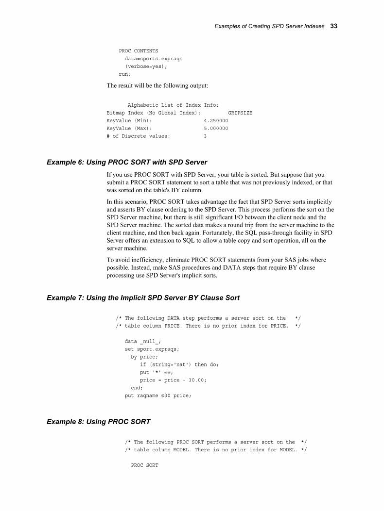
PROC CONTENTS data=sports.expraqs (verbose=yes); run;
The result will be the following output:
Alphabetic List of Index Info:Bitmap Index (No Global Index): GRIPSIZEKeyValue (Min): 4.250000KeyValue (Max): 5.000000# of Discrete values: 3
Example 6: Using PROC SORT with SPD ServerIf you use PROC SORT with SPD Server, your table is sorted. But suppose that you submit a PROC SORT statement to sort a table that was not previously indexed, or that was sorted on the table's BY column.
In this scenario, PROC SORT takes advantage the fact that SPD Server sorts implicitly and asserts BY clause ordering to the SPD Server. This process performs the sort on the SPD Server machine, but there is still significant I/O between the client node and the SPD Server machine. The sorted data makes a round trip from the server machine to the client machine, and then back again. Fortunately, the SQL pass-through facility in SPD Server offers an extension to SQL to allow a table copy and sort operation, all on the server machine.
To avoid inefficiency, eliminate PROC SORT statements from your SAS jobs where possible. Instead, make SAS procedures and DATA steps that require BY clause processing use SPD Server's implicit sorts.
Example 7: Using the Implicit SPD Server BY Clause Sort
/* The following DATA step performs a server sort on the */ /* table column PRICE. There is no prior index for PRICE. */
data _null_; set sport.expraqs; by price; if (string='nat') then do; put '*' @@; price = price - 30.00; end; put raqname @30 price;
Example 8: Using PROC SORT
/* The following PROC SORT performs a server sort on the */ /* table column MODEL. There is no prior index for MODEL. */
PROC SORT
Examples of Creating SPD Server Indexes 33

data=inventory.old_autos out=inventory.old_autos_by_model; by model; run;
34 Chapter 5 • Indexing, Sorting, and Manipulating SAS Scalable Performance Data (SPD) Server Tables
Chapter 6
SAS Scalable Performance Data (SPD) Server Dynamic Cluster Tables
Overview of Dynamic Cluster Tables . . . . . . . . . . . . . . . . . . . . . . . . . . . . . . . . . . . . . 36
Dynamic Cluster Table Structure . . . . . . . . . . . . . . . . . . . . . . . . . . . . . . . . . . . . . . . . 36
Benefits of Dynamic Cluster Tables . . . . . . . . . . . . . . . . . . . . . . . . . . . . . . . . . . . . . . 37Parallel Loading . . . . . . . . . . . . . . . . . . . . . . . . . . . . . . . . . . . . . . . . . . . . . . . . . . . . 37Fast and Economical Refreshes . . . . . . . . . . . . . . . . . . . . . . . . . . . . . . . . . . . . . . . . 38
Dynamic Cluster Table Operations . . . . . . . . . . . . . . . . . . . . . . . . . . . . . . . . . . . . . . 38Creating Dynamic Cluster Tables . . . . . . . . . . . . . . . . . . . . . . . . . . . . . . . . . . . . . . . 38Verify Dynamic Cluster Table Control Access . . . . . . . . . . . . . . . . . . . . . . . . . . . . 40Add Tables to a Dynamic Cluster Table . . . . . . . . . . . . . . . . . . . . . . . . . . . . . . . . . . 40Undo Dynamic Cluster Tables . . . . . . . . . . . . . . . . . . . . . . . . . . . . . . . . . . . . . . . . . 42Refreshing Dynamic Cluster Tables . . . . . . . . . . . . . . . . . . . . . . . . . . . . . . . . . . . . . 44Modify Dynamic Cluster Tables . . . . . . . . . . . . . . . . . . . . . . . . . . . . . . . . . . . . . . . 47Create Dynamic Clusters with Unique Indexes . . . . . . . . . . . . . . . . . . . . . . . . . . . . 48Destroy Dynamic Cluster Tables . . . . . . . . . . . . . . . . . . . . . . . . . . . . . . . . . . . . . . . 48Restoring Deleted Cluster Table Members . . . . . . . . . . . . . . . . . . . . . . . . . . . . . . . . 48
Dynamic Cluster BY Clause Optimization . . . . . . . . . . . . . . . . . . . . . . . . . . . . . . . . . 49Overview of Optimizing BY Clauses . . . . . . . . . . . . . . . . . . . . . . . . . . . . . . . . . . . . 49Combining WHERE Clauses with Dynamic Cluster BY Clause Optimization . . . . 50Dynamic Cluster BY Clause Optimization Example . . . . . . . . . . . . . . . . . . . . . . . . 50
Member Table Requirements for Creating Dynamic Cluster Tables . . . . . . . . . . . 52Overview of Table Requirements . . . . . . . . . . . . . . . . . . . . . . . . . . . . . . . . . . . . . . . 52Table Attributes . . . . . . . . . . . . . . . . . . . . . . . . . . . . . . . . . . . . . . . . . . . . . . . . . . . . 52Variable Attributes . . . . . . . . . . . . . . . . . . . . . . . . . . . . . . . . . . . . . . . . . . . . . . . . . . 53Index Attributes . . . . . . . . . . . . . . . . . . . . . . . . . . . . . . . . . . . . . . . . . . . . . . . . . . . . 54
Querying and Reading Member Tables in a Dynamic Cluster . . . . . . . . . . . . . . . . 55
Unsupported Features in Dynamic Cluster Tables . . . . . . . . . . . . . . . . . . . . . . . . . . 57
Dynamic Cluster Table Examples . . . . . . . . . . . . . . . . . . . . . . . . . . . . . . . . . . . . . . . . 57Example: Create a Dynamic Cluster Table . . . . . . . . . . . . . . . . . . . . . . . . . . . . . . . 57Example: Add Tables to a Dynamic Cluster . . . . . . . . . . . . . . . . . . . . . . . . . . . . . . 61Example: Refresh Dynamic Cluster Table with CLUSTER REPLACE . . . . . . . . . 62Example: Refresh Dynamic Cluster Table with CLUSTER
REMOVE and CLUSTER ADD . . . . . . . . . . . . . . . . . . . . . . . . . . . . . . . . . . . . . . 63Example: Undo and Refresh Dynamic Cluster Table . . . . . . . . . . . . . . . . . . . . . . . . 64
35

Overview of Dynamic Cluster TablesSPD Server is designed to meet the storage and performance demands that are associated with processing large amounts of data using SAS. As the size of the data grows, the demand to process that data increases, and storage architecture must change to keep up with business needs.
SPD Server offers dynamic cluster tables. Earlier releases of SPD Server provided a cluster table called the time-based partitioning table. To optimize the benefits of clustering, the SPD Server administrator can use dynamic clusters to partition SPD Server data tables for speed and enhanced I/O processing. Clustering is performed using metadata. When that metadata is combined with SPD Server functionality, the result is parallel processing capabilities for loading and querying data tables. Parallel processing can accelerate performance and increase the manageability, flexibility, and scalability of very large data stores.
When you use dynamic cluster tables, you can add new data or remove historical data from very large tables by accessing only the member tables that are affected by the change. You can access the individual member tables in parallel. This strategy reduces the time that you need to complete the job, and it uses simple commands. Furthermore, a complete refresh of a dynamic cluster table uses a fraction of the disk space that is needed to refresh a large traditional SAS or SPD Server table with the same amount of data.
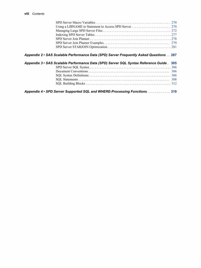
Dynamic Cluster Table StructureThe SPD Server dynamic cluster table is considered part of a hierarchy of tables that have increasing sophistication.
36 Chapter 6 • SAS Scalable Performance Data (SPD) Server Dynamic Cluster Tables

Figure 6.1 SAS Table, SPD Server Table, and SPD Server Dynamic Cluster Table Structures
• Traditional SAS tables are single files that contain data descriptors and table data. Data values are columns, and data descriptors are metadata that describes the column and data formatting that the table uses. If a traditional SAS table contains one or more indexes, they are stored in a separate file.
• SPD Server dynamic cluster tables are virtual table structures. SPD Server dynamic cluster tables consist of members. Each member is an SPD Server table. All members must share the same metadata formats and organization. SPD Server dynamic cluster tables use the metadata to manage the data that is contained in the members.
The SPD Server dynamic cluster table structure provides architecture that enables flexible loading and rapid storage and processing for very large data tables. When you use dynamic cluster tables, you can load and remove data,, and refresh tables in very large data marts in an easier and more timely manner. Dynamic cluster tables provide organizational features and performance benefits that traditional SAS tables and SPD Server tables do not have.
Benefits of Dynamic Cluster Tables
Parallel LoadingBecause dynamic cluster tables are virtual tables that consist of numerous smaller SPD Server tables, the architecture enables parallel loading and processing. Cluster table loads and refreshes are broken down into multiple tasks that can be performed concurrently. You can use separate SAS/CONNECT MP CONNECT jobs to manage the parallel loading and processing.
The scalability of parallel loading with dynamic cluster tables depends on the scalability of the server I/O and on the number of processors on the server.
Benefits of Dynamic Cluster Tables 37

Parallel loading requires multiple concurrent writes to disk. If the I/O hardware does not scale appropriately, the parallel loading process can degrade performance.
SPD Server can create multiple indexes on the same table in parallel. Index creation is a CPU-intensive process. When sufficient processing power is available, parallel index creation in SPD Server is highly scalable. The creation process for each index is threaded. A single index creation can use multiple CPUs on a server if they are available, which greatly improves performance.
Fast and Economical RefreshesRefreshing a dynamic cluster table uses a fraction of the disk space that a traditional SPD Server table with the same amount of data uses. The dynamic cluster table architecture enables you to refresh many large tables concurrently, while conserving disk and I/O resources. With very large traditional SAS or SPD Server tables, available disk space can limit the number of tables that you can refresh concurrently.
In the life cycle of data warehouses, tables can be refreshed to recapture disk space after rows have been updated or deleted. Refreshing tables can reorder data for optimized performance. However, refreshing a table can temporarily use twice the disk space of the table itself. With very large tables, disk space can be a problem when updating a data warehouse or data mart. When disk space is limited on a server, the amount of data that can be simultaneously refreshed is constrained. The amount of time that is required to load and refresh can become huge.
Because dynamic cluster tables can be quickly unbound into smaller SPD Server tables, refreshing dynamic cluster tables does not use twice the disk space of the original table itself. Instead, only twice the disk space of the largest member table in the dynamic cluster table is used.
After the dynamic cluster table is unbound, disk space equal to the first member table is required to perform a refresh. A backup of the refresh is created, and then the old version is deleted, which creates more available disk space. The refresh process repeats for each successive member table until all members in the dynamic cluster table have been refreshed and updated. Then, the member tables are merged into a dynamic cluster table again.
When a server has enough disk space and I/O resources to refresh more than one member table at a time, parallel processing provides added benefits.
Dynamic Cluster Table Operations
Creating Dynamic Cluster TablesTo create dynamic cluster tables in SPD Server, you must have a set of related SPD Server tables that you want to cluster, such as tables that contain monthly sales transactions. The SPD Server tables that you want to cluster must all be in the same domain. They must use identical table structures (columns and indexes) and compression. However, member table partition sizes and member table owners can vary. These requirements ensure the metadata compatibility that is necessary to create dynamic cluster tables in SPD Server.
After you have organized the SPD Server tables, issue a PROC SPDO command to bind the tables into a dynamic cluster table.
38 Chapter 6 • SAS Scalable Performance Data (SPD) Server Dynamic Cluster Tables
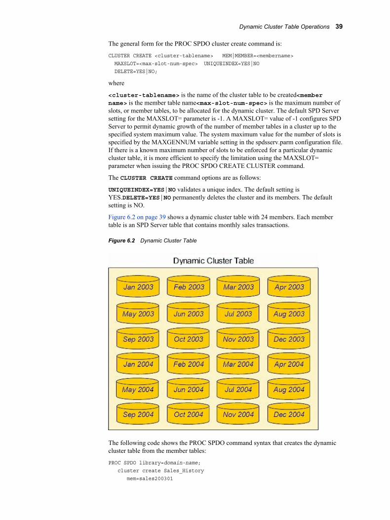
The general form for the PROC SPDO cluster create command is:
CLUSTER CREATE <cluster-tablename> MEM|MEMBER=<membername> MAXSLOT=<max-slot-num-spec> UNIQUEINDEX=YES|NO DELETE=YES|NO;
where
<cluster-tablename> is the name of the cluster table to be created<member name> is the member table name<max-slot-num-spec> is the maximum number of slots, or member tables, to be allocated for the dynamic cluster. The default SPD Server setting for the MAXSLOT= parameter is -1. A MAXSLOT= value of -1 configures SPD Server to permit dynamic growth of the number of member tables in a cluster up to the specified system maximum value. The system maximum value for the number of slots is specified by the MAXGENNUM variable setting in the spdsserv.parm configuration file. If there is a known maximum number of slots to be enforced for a particular dynamic cluster table, it is more efficient to specify the limitation using the MAXSLOT= parameter when issuing the PROC SPDO CREATE CLUSTER command.
The CLUSTER CREATE command options are as follows:
UNIQUEINDEX=YES|NO validates a unique index. The default setting is YES.DELETE=YES|NO permanently deletes the cluster and its members. The default setting is NO.
Figure 6.2 on page 39 shows a dynamic cluster table with 24 members. Each member table is an SPD Server table that contains monthly sales transactions.
Figure 6.2 Dynamic Cluster Table
The following code shows the PROC SPDO command syntax that creates the dynamic cluster table from the member tables:
PROC SPDO library=domain-name; cluster create Sales_History mem=sales200301
Dynamic Cluster Table Operations 39

mem=sales200302 mem=sales200303 mem=sales200304 mem=sales200305 mem=sales200306 mem=sales200307 mem=sales200308 mem=sales200309 mem=sales200310 mem=sales200311 mem=sales200312 mem=sales200401 mem=sales200402 mem=sales200403 mem=sales200404 mem=sales200405 mem=sales200406 mem=sales200407 mem=sales200408 mem=sales200409 mem=sales200410 mem=sales200411 mem=sales200412 quit ;
PROC SPDO uses a LIBRARY statement to identify the domain that contains the tables to be clustered. The CLUSTER CREATE syntax specifies the name of the dynamic cluster table to be created (Sales_History).
MEM= identifies the members of the dynamic cluster table. The tables in the example represent monthly sales transactions. This example uses 24 monthly sales tables for the years 2003 and 2004.
“Dynamic Cluster Table Examples” on page 57 contains more extensive code examples of creating dynamic cluster tables.
Verify Dynamic Cluster Table Control AccessYou must have SPD Server Control access to any member tables that you use in the CLUSTER CREATE or CLUSTER ADD commands. You must also have SPD Server Control access to the dynamic cluster table itself to submit a CLUSTER UNDO command. There is no restriction on table ownership if you have Control access to all the member tables. All users that have access to a domain have default Control access to tables that were created by the user Anonymous within that domain. Access control lists (ACLs) can be defined on a dynamic cluster table after it is created. The permissions that are specified in the dynamic cluster table ACL are applied when SPD Server accesses the dynamic cluster table. Any individual ACL that is defined on a member table does not apply during the time when the member table is part of a created dynamic cluster table.
Add Tables to a Dynamic Cluster TableTo add tables to a dynamic cluster table, you must have an existing dynamic cluster table. The SPD Server tables that you want to add to the dynamic cluster table must all be in the same domain as the dynamic cluster table. They must use identical table structures (columns and indexes) and compression. However, member table partition
40 Chapter 6 • SAS Scalable Performance Data (SPD) Server Dynamic Cluster Tables

sizes and member table owners can vary. These requirements ensure the metadata compatibility that is required to add to a dynamic cluster table.
After the SPD Server tables are organized, issue a PROC SPDO command to add the tables to an existing dynamic cluster table.
The general form of the PROC SPDO CLUSTER ADD command is as follows:
CLUSTER ADD <cluster-tablename> MEM|MEMBER=<membername>;
where
<cluster-tablename> is the name of the cluster table to be created<member name> is the member table name.
Figure 6.3 on page 41 shows sales tables for the first six months of 2005. These tables are set up to be added to the dynamic cluster table that contains monthly sales transactions data for 2003 and 2004, which was reviewed in “Creating Dynamic Cluster Tables” on page 38.
Figure 6.3 New Monthly Data to Add to an Existing Dynamic Cluster Table
The following code shows the PROC SPDO command syntax that adds the new tables to an existing dynamic cluster table:
PROC SPDO library=domain-name; cluster add Sales_History mem=sales200501 mem=sales200502 mem=sales200503 mem=sales200504 mem=sales200505 mem=sales200506;quit;
Dynamic Cluster Table Operations 41

PROC SPDO uses a LIBRARY statement to identify the domain that contains the existing dynamic cluster table that you want to add to. The CLUSTER ADD syntax specifies the name of the dynamic cluster table that you want to add to (Sales_History).
MEM= identifies the member tables of the table to be added to the existing dynamic cluster table.
In Figure 6.4 on page 42, six tables that include monthly sales transactions for the first half of 2005 are set up to be added to the existing dynamic cluster table that contains 2003 and 2004 sales transactions data.
Figure 6.4 Adding Member Tables to a Dynamic Cluster Table
“Dynamic Cluster Table Examples” on page 57 contains more extensive code examples of adding to a dynamic cluster table.
Undo Dynamic Cluster TablesTo undo a dynamic cluster table, you must have an existing dynamic cluster table. Undoing the dynamic cluster table reverts the table back to its unbound SPD Server tables. You must undo a dynamic cluster table in order to remove a specific member table from a dynamic cluster table, to add data to a specific member table in the dynamic cluster table, or to completely refresh a specific member table that belongs to the dynamic cluster table.
The general form of the PROC SPDO CLUSTER UNDO command is as follows:
CLUSTER UNDO <cluster-tablename> ;
where<cluster-tablename> is the name of the cluster table to undo.
Figure 6.5 on page 43 shows a dynamic cluster table with 30 members. Each member contains monthly sales transactions for the years 2003 and 2004, and part of 2005.
42 Chapter 6 • SAS Scalable Performance Data (SPD) Server Dynamic Cluster Tables
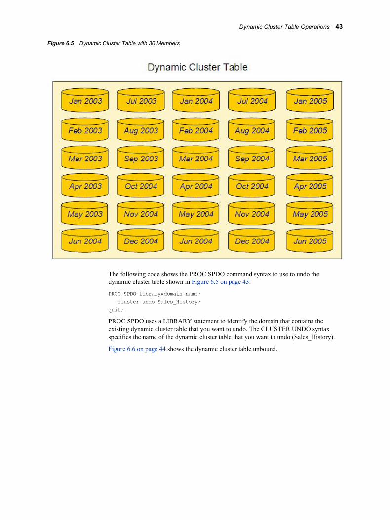
Figure 6.5 Dynamic Cluster Table with 30 Members
The following code shows the PROC SPDO command syntax to use to undo the dynamic cluster table shown in Figure 6.5 on page 43:
PROC SPDO library=domain-name; cluster undo Sales_History;quit;
PROC SPDO uses a LIBRARY statement to identify the domain that contains the existing dynamic cluster table that you want to undo. The CLUSTER UNDO syntax specifies the name of the dynamic cluster table that you want to undo (Sales_History).
Figure 6.6 on page 44 shows the dynamic cluster table unbound.
Dynamic Cluster Table Operations 43
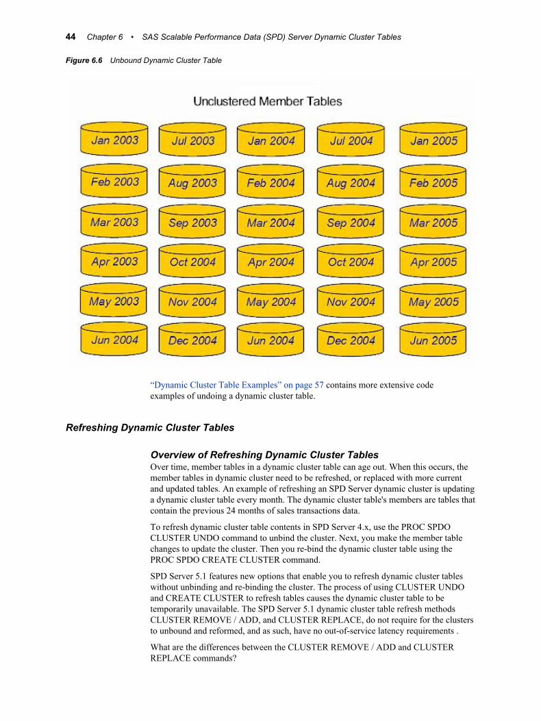
Figure 6.6 Unbound Dynamic Cluster Table
“Dynamic Cluster Table Examples” on page 57 contains more extensive code examples of undoing a dynamic cluster table.
Refreshing Dynamic Cluster Tables
Overview of Refreshing Dynamic Cluster TablesOver time, member tables in a dynamic cluster table can age out. When this occurs, the member tables in dynamic cluster need to be refreshed, or replaced with more current and updated tables. An example of refreshing an SPD Server dynamic cluster is updating a dynamic cluster table every month. The dynamic cluster table's members are tables that contain the previous 24 months of sales transactions data.
To refresh dynamic cluster table contents in SPD Server 4.x, use the PROC SPDO CLUSTER UNDO command to unbind the cluster. Next, you make the member table changes to update the cluster. Then you re-bind the dynamic cluster table using the PROC SPDO CREATE CLUSTER command.
SPD Server 5.1 features new options that enable you to refresh dynamic cluster tables without unbinding and re-binding the cluster. The process of using CLUSTER UNDO and CREATE CLUSTER to refresh tables causes the dynamic cluster table to be temporarily unavailable. The SPD Server 5.1 dynamic cluster table refresh methods CLUSTER REMOVE / ADD, and CLUSTER REPLACE, do not require for the clusters to unbound and reformed, and as such, have no out-of-service latency requirements .
What are the differences between the CLUSTER REMOVE / ADD and CLUSTER REPLACE commands?
44 Chapter 6 • SAS Scalable Performance Data (SPD) Server Dynamic Cluster Tables
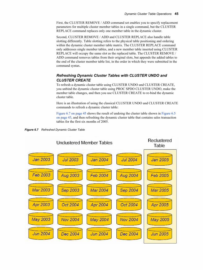
First, the CLUSTER REMOVE / ADD command set enables you to specify replacement parameters for multiple cluster member tables in a single command, but the CLUSTER REPLACE command replaces only one member table in the dynamic cluster.
Second, CLUSTER REMOVE / ADD and CLUSTER REPLACE also handle table slotting differently. Table slotting refers to the physical table positioning and ordering within the dynamic cluster member table matrix. The CLUSTER REPLACE command only addresses single member tables, and a new member table inserted using CLUSTER REPLACE will occupy the same slot as the replaced table. The CLUSTER REMOVE / ADD command removes tables from their original slots, but appends the added tables to the end of the cluster member table list, in the order in which they were submitted in the command syntax.
Refreshing Dynamic Cluster Tables with CLUSTER UNDO and CLUSTER CREATETo refresh a dynamic cluster table using CLUSTER UNDO and CLUSTER CREATE, you unbind the dynamic cluster table using PROC SPDO CLUSTER UNDO, make the member table changes, and then you use CLUSTER CREATE to re-bind the dynamic cluster table.
Here is an illustration of using the classical CLUSTER UNDO and CLUSTER CREATE commands to refresh a dynamic cluster table:
Figure 6.7 on page 45 shows the result of undoing the cluster table shown in Figure 6.5 on page 43, and then refreshing the dynamic cluster table that contains sales transaction tables for the first six months of 2005.
Figure 6.7 Refreshed Dynamic Cluster Table
Dynamic Cluster Table Operations 45
“Dynamic Cluster Table Examples” on page 57 contains a more extensive code example of unbinding a dynamic cluster table and refreshing it by re-creating it with different member tables.
Refreshing Dynamic Cluster Tables with CLUSTER REMOVE and CLUSTER ADDThe SPD Server PROC SPDO CLUSTER REMOVE and CLUSTER ADD commands enable you to refresh dynamic cluster tables without unbinding and re-binding the cluster, and without making the dynamic cluster table temporarily unavailable during refactoring.
The CLUSTER REMOVE / ADD command set enables you to specify replacement member tables for one or more member tables in a dynamic cluster that have aged out or are otherwise not wanted. The CLUSTER REMOVE / ADD command removes old member tables from their original position in the cluster member table list, and appends new updated tables to the end of the cluster member table list, in the order in which they were submitted in the command syntax.
The PROC SPDO CLUSTER REMOVE command removes one or more member tables from a dynamic cluster. When a cluster member table is removed, users that currently have that particular cluster open for Read access will not see the change, until a subsequent open or reopen of the cluster is performed by the user, after the remove command has completed. The same is true for the CLUSTER ADD command: changes are not reflected until the cluster is opened or reopened after the CLUSTER ADD processing is complete.
A cluster member table that has been removed from a cluster becomes visible as a simple SPD Server table, but the table remains in a read-only state. If there is a need to update a member table that has been removed from a cluster, use the CLUSTER FIX MEMBER “Restoring Deleted Cluster Table Members” on page 48 command to restore the member table to a writable state.
The general form of the PROC SPDO CLUSTER REMOVE command is as follows:
CLUSTER REMOVE <cluster-tablename> MEM= <membername_1> MEM= <membername_2> ... MEM= <membername_n> ;
where
<cluster-tablename>is the name of the dynamic cluster to be edited
<membername_n>is a list of one or more tables to be removed from the edited dynamic cluster.
The general form of the PROC SPDO CLUSTER ADD command is as follows:
CLUSTER ADD <cluster-tablename> MEM= <membername_1> MEM= <membername_2> ... MEM= <membername_n> ;
where
46 Chapter 6 • SAS Scalable Performance Data (SPD) Server Dynamic Cluster Tables
<cluster-tablename>is the name of the dynamic cluster to be edited
<membername_n>is a list of one or more tables to be removed from the edited dynamic cluster.
Refreshing Dynamic Cluster Tables with CLUSTER REPLACELike the CLUSTER REMOVE and CLUSTER ADD command set, the SPD Server PROC SPDO CLUSTER REPLACE command enables you to refresh dynamic cluster tables without unbinding and re-binding the cluster.
The CLUSTER REPLACE command enables you to specify a replacement member table for a single member table in a dynamic cluster that has aged out or is otherwise not wanted. The CLUSTER REPLACE command removes the old member table from its original position in the cluster member table list, and replaces the old member table with the new member table in the same slot (or cluster position).
The PROC SPDO CLUSTER REPLACE command replaces one member table from a dynamic cluster. When a cluster member table is removed, users that currently have that particular cluster open for Read access will not see the change, until a subsequent open or reopen of the cluster is performed by the user, after the replace command has completed.
A cluster member table that has been replaced in a cluster becomes visible as a simple SPD Server table, but the table remains in a read-only state. If there is a need to update a member table that has been replaced from a cluster, use the CLUSTER FIX MEMBER“Restoring Deleted Cluster Table Members” on page 48 command to restore the member table to a writable state.
The general form of the CLUSTER REPLACE command is as follows:
CLUSTER REPLACE <cluster-tablename> OLDMEMBER|OLDMEM= <member-name> NEWMEMBER|NEWMEM= <member-name> ;
where
<cluster-tablename> is the name of the cluster table that you want to replace members inOLDMEMBER|OLDMEM= is the name of the old member table that you want to remove from the cluster tableNEWMEMBER|NEWMEM= is the name of the new member table that you want to insert into the cluster table.
Modify Dynamic Cluster TablesPROC SPDO uses a CLUSTER MODIFY command to modify a dynamic cluster table.
The general form for the PROC SPDO CLUSTER MODIFY command is as follows:
CLUSTER MODIFY <cluster-tablename> MINMAXVARLIST=(<<varname1> <varname2> <varname3> ...>);
where<cluster-tablename> is the name of the cluster table to be created<<varname1> <varname2> <varname3> ...> are the names of the minmax variables to be added.
The CLUSTER MODIFY command sets the MINMAXVARLIST attribute on variables that belong to an existing dynamic cluster. The variable names that you specify on the CLUSTER MODIFY command must exist in the dynamic cluster tables. The variables
Dynamic Cluster Table Operations 47
must not have a preexisting MINMAXVARLIST setting. When the SPD Server runs the CLUSTER MODIFY command, it unclusters the dynamic cluster table and makes the variable modifications to the individual member tables. The dynamic cluster table is re-created after the variable modifications have completed. You must have Control access and Exclusive access to the dynamic cluster table in order to run the CLUSTER MODIFY command. SPD Server performs a full table scan to initialize the MINMAXVARLIST values in each member table. As a result, the processor time required for the CLUSTER MODIFY command is directly related to the sizes of the tables that belong to the dynamic cluster table. If an error occurs while the CLUSTER MODIFY command is running, the dynamic cluster table cannot be re-created, and you need to manually re-create it by issuing the CLUSTER CREATE command.
Create Dynamic Clusters with Unique IndexesUse the UNIQUEINDEX option on the CLUSTER CREATE command in PROC SPDO to specify whether the unique indexes that are defined in the member tables should be validated and marked as unique in the dynamic cluster table. If you set the UNIQUEINDEX option to NO, then unique indexes are not validated, and the dynamic cluster table metadata does not mark the indexes as unique within the cluster. If you do not specify the UNIQUEINDEX option, then the default setting YES is used. In this case, the indexes are validated and marked as unique within the cluster. The processing that is required to validate the unique indexes depends on the number of rows in the tables. Processing can take considerable time for larger tables. If you choose to use the validation process but the indexes are not unique, the CLUSTER CREATE command fails.
CLUSTER CREATE clusternameMEM=member_table_1MEM=member_table_2 ...MEM=member_table_nUNIQUEINDEX=<yes|no>;
Destroy Dynamic Cluster TablesYou use the PROC SPDO CLUSTER DESTROY command when you want to delete or destroy an existing cluster table. The general form of the PROC SPDO CLUSTER DESTROY command is as follows:
CLUSTER DESTROY <cluster-tablename> ;
where<cluster-tablename> is the name of the cluster table that you want to destroy.
The CLUSTER DESTROY command is valid only when used on clusters that were created with the DELETE=YES option configured.
Restoring Deleted Cluster Table MembersYou use the PROC SPDO CLUSTER FIX command when you need to restore removed or replaced cluster member tables to a writable state. The general form for the PROC SPDO CLUSTER FIX command is as follows:
CLUSTER FIX <member-tablename> ;
where<member-tablename> is the name of the member table that you want to repair.
48 Chapter 6 • SAS Scalable Performance Data (SPD) Server Dynamic Cluster Tables
Dynamic Cluster BY Clause Optimization
Overview of Optimizing BY ClausesWhen you use SPD Server dynamic clusters, you can create huge data sets. If a SAS job needs to manipulate a huge data set, you can sort the data sets for more efficient processing. Traditional processing of huge data sets can overuse or overwhelm available resources. Insufficient run-time or processor resources can prohibit you from running full table scans and manipulating table rows, which are required to sort huge data sets for subsequent processing.
SPD Server provides dynamic cluster BY clause optimization to reduce the need for a large amount of processor resources when evaluating BY clauses. Dynamic cluster BY clause optimization uses SPD Server to join individually created SPD Server member data sets so that the data sets appear to be a single data set, but the individual member data sets are also kept intact. Dynamic cluster BY clause optimization uses the SORTEDBY metadata of the member data sets to bypass most of the sorting that is required to perform the implicit BY clause ordering. SPD Server uses the SORTEDBY metadata of each member data set to merge the member data sets in the dynamic cluster in order by each member data set's order. No additional SPD Server workspace is required, and the ordered data set records are returned quickly because the member data sets do not need to be sorted.
To use dynamic cluster BY clause optimization, you need to build the dynamic cluster table a specific way. All of the member tables in your dynamic cluster table need to be sorted by the same columns that you use in the BY clause. When you build your dynamic cluster table from member tables that are presorted by your BY clause columns, your dynamic cluster table can use the BY clause optimization.
When you run a BY clause that matches the SORTEDBY column order of the member tables of the dynamic cluster table, SPD Server processes the BY clause without using sort workspace and does not experience first-record latency. SPD Server uses the presorted member tables to perform an instantaneous interleave. Because dynamic cluster BY clause optimization uses the presorted member tables, you can perform operations on huge data sets that would be impossible to handle otherwise.
For example, suppose your system has sufficient CPU, memory and workspace resources to sort a 50 GB data set in a reasonable amount of time. However, suppose this system accumulates 50 GB of new data every month. After 12 months, the data set requires 600 GB of storage. The system cannot sort 600 GB of data to process queries that are based on the previous 12-month period. To use dynamic cluster BY clause optimization in this situation:
1. Create a dynamic cluster table from the twelve 50 GB member tables. You have a 600 GB dynamic cluster table.
2. Store data for each successive month in an SPD Server member table.
3. Sort each table and add it to the 600 GB dynamic cluster table.
4. Use dynamic cluster BY clause optimization to run SAS steps that use BY clauses on the 600 GB dynamic cluster table.
For example, you can run a DATA step MERGE statement that uses the dynamic cluster table as the master source for the MERGE statement. The BY clause from the MERGE statement triggers the dynamic cluster BY clause optimization. The
Dynamic Cluster BY Clause Optimization 49

operation completes in the time that it takes to interleave the individual member tables. The process uses no SPD Server workspace and does not cause any implicit BY sort delays.
Dynamic cluster BY clause optimization is triggered when all member tables have an applicable SORTEDBY ordering for the BY clause that is asserted. When the SORTEDBY ordering is strong (validated), SPD Server does not verify the order of BY variables that are returned from the member table. When the SORTEDBY ordering is weak (such as from a SORTEDBY assertion that was a data set option), SPD Server verifies the order of BY variables that are returned from the member table. If SPD Server detects an invalid BY variable order, it terminates the BY clause and displays the following error message:
ERROR: Clustered BY member violates weaksort order during merge.
Combining WHERE Clauses with Dynamic Cluster BY Clause Optimization
You can use dynamic cluster BY clause optimization to combine BY clause optimization with certain WHERE clauses on dynamic cluster tables. SPD Server must be able to determine whether the WHERE clause is trivially true or trivially false for each member table in the dynamic cluster table. To be trivially true, a WHERE clause must find the clause condition to be true for every row in the member table. To be trivially false, a WHERE clause must find the clause condition to be false for every row in the member table.
SPD Server keeps metadata about indexed values that are in dynamic cluster table member tables. If SPD Server can determine whether the WHERE clause criteria is true or false, based on the dynamic cluster table's member table metadata, WHERE clause optimization is possible on a member-by-member basis for the entire dynamic cluster table. Suppose that member tables of a dynamic cluster table all have an index on the column QUARTER (1=JAN-MAR, 2=APR-JUN, 3=JUL-SEP, 4=OCT-DEC). Suppose you need to run a DATA step MERGE statement that uses the expression WHERE QUARTER=2. Because the QUARTER column is indexed in all of the member tables, SPD Server uses BY clause optimization to determine that the WHERE clause is trivially true. SPD Server evaluates the expression only on the member tables for April, May, and June, and does not use any SPD Server workspace. If the WHERE clause is determined to be trivially true or trivially false for each member table of the dynamic cluster table in advance, BY clause optimization performs BY processing only on the appropriate member tables.
Dynamic Cluster BY Clause Optimization ExampleConsider a database of medical patient insurance claims that contains quarterly claims data sets that are named ClaimsQ1, ClaimsQ2, ClaimsQ3, and ClaimsQ4. The following code does these tasks:
1. Sorts each quarterly claims table into columns that are named PatID (for patient ID) and ClaimID (for claim ID).
2. Combines the member tables into a dynamic cluster table that is named ClaimsAll.
DATA SPDS.ClaimsQ1;...run;
50 Chapter 6 • SAS Scalable Performance Data (SPD) Server Dynamic Cluster Tables
DATA SPDS.ClaimsQ2;...run;
PROC SORT DATA=SPDS.ClaimsQ1; BY PatID ClaimID;run;
PROC SORT DATA=SPDS.ClaimsQ2; BY PatID ClaimID;run;
PROC SPDO LIB=SPDS;create cluster ClaimsAll;quit;
The following DATA step MERGE statement is submitted to the ClaimsAll dynamic cluster table:
DATA SPDS.ToAdd SPDS.ToUpdate;MERGE SPDS.NewOnes(IN=NEW1) SPDS.ClaimsAll(IN=OLD1);BY PatID ClaimID;
SELECT;WHEN(NEW1 and OLD1) DO; OUTPUT SPDS.ToUpdate; end;WHEN(NEW1 and not OLD1) DO; OUTPUT SPDS.ToAdd; end;run;
If ClaimsAll was not a dynamic cluster table, the DATA step MERGE statement would create an implicit sort from the BY clause on the respective SPD Server data sets. However, ClaimsAll is a dynamic cluster table with member tables that are presorted. As a result, dynamic cluster BY clause optimization uses BY clause processing to merge the sorted member tables instantaneously without using any SPD Server workspace or creating any delays. The example merges the transaction data named NewOnes into new rows that are appended to the data for the next quarter.
The member data sets ClaimsQ1 and ClaimsQ2 are indexed on the column Claim_Date:
DATA SPDS.RepClaims; SET SPDS.ClaimsAll; WHERE Claim_Date BETWEEN '01JAN2007' and '31MAR2007'; BY PatID ClaimID;run;
The WHERE clause determines whether each member table is true or false for each quarter. The WHERE clause is trivially true for the data set ClaimsQ1 because the WHERE clause is true for all dates in the first quarter. The WHERE clause is trivially false for the data set ClaimsQ2 because the WHERE clause is false for all dates in the second quarter. BY clause optimization determines that the member table ClaimsQ1 will be processed because the WHERE clause is true for all of the rows of the ClaimsQ1 table. BY clause optimization skips the data set ClaimsQ2 because the WHERE clause is false for all of the rows of the ClaimsQ2 table.
Dynamic Cluster BY Clause Optimization 51

Suppose that the Claim_Date range is changed in the WHERE clause:
DATA SPDS.RepClaims; SET SPDS.ClaimsAll; WHERE Claim_Date BETWEEN '05JAN2007' and '28JUN2007'; BY PatID ClaimID;run;
When the new WHERE clause is evaluated, it is not trivially true for member tables ClaimsQ1 or ClaimsQ2. The WHERE clause is not trivially false for member tables ClaimsQ1 or ClaimsQ2, either. The WHERE clause calls dates that exist in portions of the member table ClaimsQ1, and it calls dates that exist in portions of the member table ClaimsQ2. The dates in the WHERE clause do not match all of the dates that exist in the member table ClaimsQ1, and they do not match all of the dates that exist in the member table ClaimsQ2. The dates in the WHERE clause are not totally exclusive of the dates that exist in the member tables ClaimsQ1 or ClaimsQ2. As a result, SPD Server does not use BY clause optimization when it runs the code.
Member Table Requirements for Creating Dynamic Cluster Tables
Overview of Table RequirementsWhen you create a dynamic cluster table, all of the member tables must have matching table, variable, and index attributes. If there are attribute mismatches, the dynamic cluster table is not created, and SPD Server displays the following error message:
ERROR: Member table not compatible with other cluster members. Compare CONTENTS.
A more detailed error message is written to the SPD Server log. The SPD Server log lists which attribute is mismatched in the member table. All of the member table attributes that are described in the following topics must match in order for SPD Server to successfully create a dynamic cluster table.
• “Table Attributes” on page 52
• “Variable Attributes” on page 53
• “Index Attributes” on page 54
Table AttributesThe following table attributes must match in all member tables to successfully create a dynamic cluster table:
CONSTRAINTwhere constraint
DISKCOMPcompression algorithm
DSORGdata set organization
DS_ROLEdata set option for ROLE
52 Chapter 6 • SAS Scalable Performance Data (SPD) Server Dynamic Cluster Tables
DSTYPESAS data-set type
ENCODING_CEIencoding CEI for NLS (for compressed tables)
FLAGS• compressed data set
• encrypted data set
• backup data set
• NLS variables in data set
• MINMAXVARLIST variables in data set
• SAS encryption password in data set
IOBLOCKSIZEI/O block size
IOBLOCKFACTORI/O block factor
LANGdata set language tag
LTYPEdata set language type tag
NINDEXESnumber of indexes
NVARnumber of columns
OBSLENobservation record length
SASPWSAS encryption password
SEMTYPEdata set semantic type
Variable AttributesThe following variable attributes must match in all member tables to successfully create a dynamic cluster table:
NAMEvariable name
LABELvariable label
NFORMvariable format
NIFORMvariable informat
NPOSvariable offset in record
Member Table Requirements for Creating Dynamic Cluster Tables 53

NVAROvariable number in record
NLNGvariable length
NPRECvariable precision
FLAGS• NLS encoding supported
• MINMAXVARLIST variable
NFLformat length
NFDformat decimal places
NIFLinformat length
NIFDinformat precision
NSCALEscale for fixed-point decimal
NTATTRvariable type attributes
TYPEvariable type
SUBTYPEvariable subtype
SORTvariable sorted status
NTYPE2variable extended type code
Index AttributesThe following index attributes must match in all member tables to successfully create a dynamic cluster table:
NAMEindex name
TYPEindex type
KEYFLAGS• unique index
• nomiss index
LENGTHindex length
NVARnumber of variables in index
54 Chapter 6 • SAS Scalable Performance Data (SPD) Server Dynamic Cluster Tables
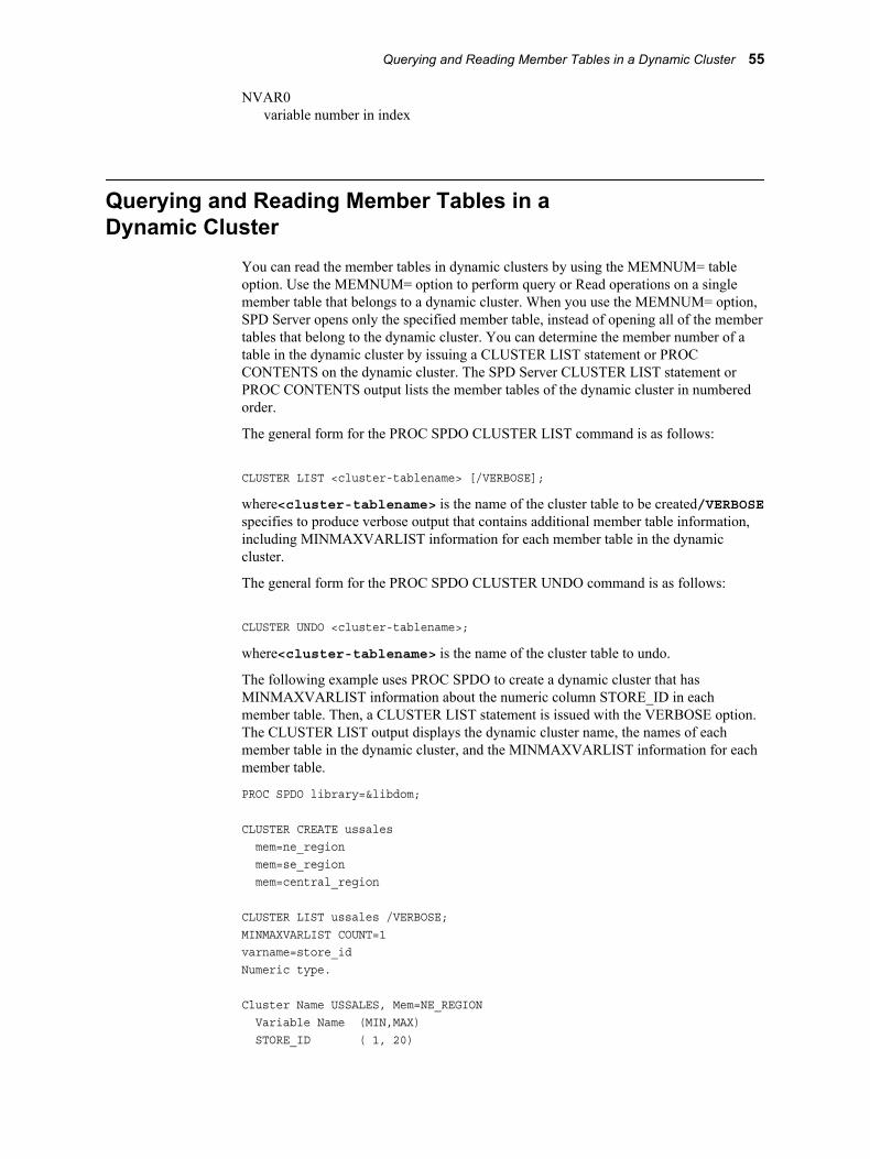
NVAR0variable number in index
Querying and Reading Member Tables in a Dynamic Cluster
You can read the member tables in dynamic clusters by using the MEMNUM= table option. Use the MEMNUM= option to perform query or Read operations on a single member table that belongs to a dynamic cluster. When you use the MEMNUM= option, SPD Server opens only the specified member table, instead of opening all of the member tables that belong to the dynamic cluster. You can determine the member number of a table in the dynamic cluster by issuing a CLUSTER LIST statement or PROC CONTENTS on the dynamic cluster. The SPD Server CLUSTER LIST statement or PROC CONTENTS output lists the member tables of the dynamic cluster in numbered order.
The general form for the PROC SPDO CLUSTER LIST command is as follows:
CLUSTER LIST <cluster-tablename> [/VERBOSE];
where<cluster-tablename> is the name of the cluster table to be created/VERBOSE specifies to produce verbose output that contains additional member table information, including MINMAXVARLIST information for each member table in the dynamic cluster.
The general form for the PROC SPDO CLUSTER UNDO command is as follows:
CLUSTER UNDO <cluster-tablename>;
where<cluster-tablename> is the name of the cluster table to undo.
The following example uses PROC SPDO to create a dynamic cluster that has MINMAXVARLIST information about the numeric column STORE_ID in each member table. Then, a CLUSTER LIST statement is issued with the VERBOSE option. The CLUSTER LIST output displays the dynamic cluster name, the names of each member table in the dynamic cluster, and the MINMAXVARLIST information for each member table.
PROC SPDO library=&libdom;
CLUSTER CREATE ussales mem=ne_region mem=se_region mem=central_region CLUSTER LIST ussales /VERBOSE;MINMAXVARLIST COUNT=1varname=store_idNumeric type.
Cluster Name USSALES, Mem=NE_REGION Variable Name (MIN,MAX) STORE_ID ( 1, 20)
Querying and Reading Member Tables in a Dynamic Cluster 55

Cluster Name USSALES, Mem=SE_REGION Variable Name (MIN,MAX) STORE_ID ( 60, 70)
Cluster Name USSALES, Mem=CENTRAL_REGION Variable Name (MIN,MAX) STORE_ID ( 60, 70)
NOTE: The maximum number of possible slots is 6.
You can specify an integer value n as an argument for the MEMNUM= table option to select the nth member of the table, or you can use the argument LASTCLUSTERMEMBER. When you use the LASTCLUSTERMEMBER argument with MEMNUM=, SPD Server selects the last member of the dynamic cluster table without counting the members to determine the n value of the last member.
The following example uses the MEMNUM= table option to query the member table sales200504, which belongs to the dynamic cluster table sales_history:
PROC SPDO library=&domain; CLUSTER CREATE sales_history mem=sales200501 mem=sales200502 mem=sales200503 mem=sales200504 mem=sales200505 mem=sales200506; quit;
PROC PRINT data=&domain..sales_history (MEMNUM=4); WHERE salesdate=30Apr2005; run;
The following code uses the MEMNUM= table option to query the last member table in the dynamic cluster table sales200506:
PROC SPDO library=&domain; CLUSTER CREATE sales_history mem=sales200501 mem=sales200502 mem=sales200503 mem=sales200504 mem=sales200505 mem=sales200506; quit;
PROC PRINT data&domain..sales_history (MEMNUM=LASTCLUSTERMEMBER); WHERE salesdate=15Jun2005; run;
56 Chapter 6 • SAS Scalable Performance Data (SPD) Server Dynamic Cluster Tables

Unsupported Features in Dynamic Cluster TablesBecause of differences in the load and read structures for dynamic cluster tables, the following standard features that are available in SAS tables and SPD Server tables are currently not supported in SPD Server 5.1:
• You cannot directly append or update data in a dynamic cluster table. To append new member tables to a dynamic cluster table, create the new member tables with the data to append, and then use the CLUSTER ADD on page 40 commands to add the new member to the table.
• To update an individual member table in a dynamic cluster table, create the new member table with the data to append, and then use the CLUSTER REPLACE on page 47 command to replace the old member table with the new one.
• To refresh a dynamic cluster table by removing numerous old member tables and replacing them with new member tables, create the new member tables with the data to append, and then use the CLUSTER ADD and CLUSTER REMOVE on page 46 commands to first remove and then replace the old member tables with new ones.
• You can still use classic SPD Server PROC SPDO CLUSTER UNDO and CLUSTER CREATE commands to refresh the member tables in a dynamic cluster table by unbinding the dynamic cluster table and then re-binding it back together using new member tables, However, this process temporarily makes the cluster table unavailable to other users, unlike the process used by the CLUSTER REPLACE and CLUSTER REMOVE / ADD commands.
• Record-level locking is not allowed.
• The SPD Server backup and restore utilities are not available.
If a task for a dynamic cluster table requires one of these features, you should uncluster the dynamic cluster table and create standard SPD Server tables.
Dynamic Cluster Table ExamplesThe following four examples show all of the fundamental operations that are required to use dynamic cluster tables.
Example: Create a Dynamic Cluster TableThe following example creates a dynamic cluster table named Sales_History. The example uses SPD Server tables from the domain Motorcycle.
The first part of the example generates dummy transaction data that is used in the rest of the example. The code creates tables for monthly sales data for 2004 and for the first 6 months of 2005, and then sorts and indexes the data. Next, the code binds twelve individual SPD Server tables for monthly motorcycle sales during 2004 to the dynamic cluster table named Sales_History.
/* declare macro variables that will be used to *//* generate dummy transaction data */%macro var (varout,dist,card,seed,peak); %put &dist; &card; &seed; ;
Dynamic Cluster Table Examples 57

%local var1;
if upcase("&dist;")='RANUNI' then do; &varout; = int(ranuni(&seed;)*&card;)+1; end; else if upcase("&dist;")='RANTRI' then do; *%let vartri=%substr("&dist;",5,2)&card; ; *&varout;=int(rantri(&seed;,&peak;)*&card;)+1; &varout;=int(rantri(&seed;,&peak;)*&card;)+1; end;%mend;
%macro linkvar (varin,varout,devisor); &varout;=int(&varin;/&devisor;);%mend;
/* declare main vars */%let domain=motorcycle;%let host=kaboom;%let port=5200;%let spdssize=256M;%let spdsiasy=YES;
LIBNAME &domain; sasspds "&domain;" server=&host..;&port; user='anonymous' ip=YES;
/* generate monthly sales data tables for *//* 2004 and the first six months of 2005 */data &domain..sales200401; &domain..sales200402; &domain..sales200403; &domain..sales200404; &domain..sales200405; &domain..sales200406; &domain..sales200407; &domain..sales200408; &domain..sales200409; &domain..sales200410; &domain..sales200411; &domain..sales200412; &domain..sales200501; &domain..sales200502; &domain..sales200503; &domain..sales200504; &domain..sales200505; &domain..sales200506; ;
drop seed bump1 bump2 random_dist;
58 Chapter 6 • SAS Scalable Performance Data (SPD) Server Dynamic Cluster Tables

seed=int(time());
/* format the dummy transaction data */format trandate shipdate paiddate yymmdd10. ;
put seed; do transact=1 to 5000; %var (customer,ranuni,100000,seed,1);
%linkvar (customer,zipcode,10); %linkvar (customer,agent,20); %linkvar (customer,mktseg,10000); %linkvar (agent,state,100); %linkvar (agent,branch,25); %linkvar (state,region,10);
%var (item_number,ranuni,15000,seed,1);
%var (trandate,ranuni,577,seed,1); trandate=trandate+16071;
%var (bump1,ranuni,20,seed,.1); shipdate=trandate+bump1;
%var (bump2,rantri,30,seed,.5); paiddate=trandate+bump2;
%var (units,ranuni,100,seed,1); %var (trantype,ranuni,10,seed,1); %var (amount,rantri,50,seed,.5); amount=amount+25;
random_dist=ranuni ('03feb2005'd);
/* sort the dummy transaction data into */ /* monthly sales data tables */
if '01jan2004'd <= trandate <= '31jan2004'd then output &domain..sales200401; ;
else if '01feb2004'd <= trandate <= '28feb2004'd then output &domain..sales200402; ;
else if '01mar2004'd <= trandate <= '31mar2004'd then output &domain..sales200403; ;
else if '01apr2004'd <= trandate <= '30apr2004'd then output &domain..sales200404; ;
else if '01may2004'd <= trandate <= '31may2004'd then output &domain..sales200405; ;
else if '01jun2004'd <= trandate <= '30jun2004'd then output &domain..sales200406; ;
Dynamic Cluster Table Examples 59

else if '01jul2004'd <= trandate <= '31jul2004'd then output &domain..sales200407; ;
else if '01aug2004'd <= trandate <= '31aug2004'd then output &domain..sales200408; ;
else if '01sep2004'd <= trandate <= '30sep2004'd then output &domain..sales200409; ;
else if '01oct2004'd <= trandate <= '31oct2004'd then output &domain..sales200410; ;
else if '01nov2004'd <= trandate <= '30nov2004'd then output &domain..sales200411; ;
else if '01dec2004'd <= trandate <= '31dec2004'd then output &domain..sales200412; ;
else if '01jan2005'd <= trandate <= '31jan2005'd then output &domain..sales200501; ;
else if '01feb2005'd <= trandate <= '28feb2005'd then output &domain..sales200502; ;
else if '01mar2005'd <= trandate <= '31mar2005'd then output &domain..sales200503; ;
else if '01apr2005'd <= trandate <= '30apr2005'd then output &domain..sales200504; ;
else if '01may2005'd <= trandate <= '31may2005'd then output &domain..sales200505; ;
else if '01jun2005'd <= trandate <= '31jun2005'd then output &domain..sales200506; ; end ;run ;
/* index the transaction data in the *//* monthly sales data tables */%macro indexit (yrmth); PROC DATASETS library=&domain; nolist; modify sales&yrmth; ; index create transact customer agent state branch trandate; quit;%mend;
%let spdsiasy=YES;
%indexit (200401);%indexit (200402);%indexit (200403);%indexit (200404);%indexit (200405);%indexit (200406);%indexit (200407);
60 Chapter 6 • SAS Scalable Performance Data (SPD) Server Dynamic Cluster Tables
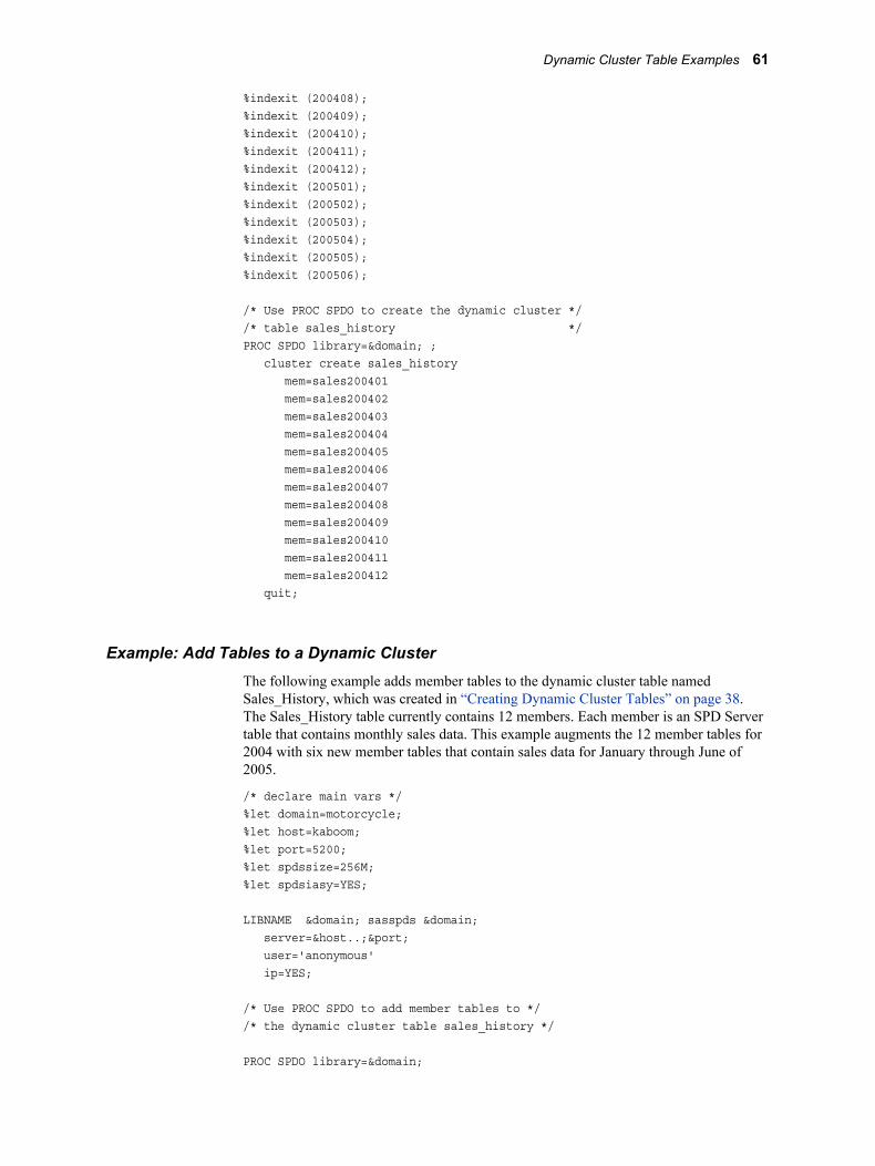
%indexit (200408);%indexit (200409);%indexit (200410);%indexit (200411);%indexit (200412);%indexit (200501);%indexit (200502);%indexit (200503);%indexit (200504);%indexit (200505);%indexit (200506);
/* Use PROC SPDO to create the dynamic cluster *//* table sales_history */PROC SPDO library=&domain; ; cluster create sales_history mem=sales200401 mem=sales200402 mem=sales200403 mem=sales200404 mem=sales200405 mem=sales200406 mem=sales200407 mem=sales200408 mem=sales200409 mem=sales200410 mem=sales200411 mem=sales200412 quit;
Example: Add Tables to a Dynamic ClusterThe following example adds member tables to the dynamic cluster table named Sales_History, which was created in “Creating Dynamic Cluster Tables” on page 38. The Sales_History table currently contains 12 members. Each member is an SPD Server table that contains monthly sales data. This example augments the 12 member tables for 2004 with six new member tables that contain sales data for January through June of 2005.
/* declare main vars */%let domain=motorcycle;%let host=kaboom;%let port=5200;%let spdssize=256M;%let spdsiasy=YES;
LIBNAME &domain; sasspds &domain; server=&host..;&port; user='anonymous' ip=YES;
/* Use PROC SPDO to add member tables to */ /* the dynamic cluster table sales_history */
PROC SPDO library=&domain;
Dynamic Cluster Table Examples 61

cluster add sales_history mem=sales200501 mem=sales200502 mem=sales200503 mem=sales200504 mem=sales200505 mem=sales200506;quit;
/* Verify the presence of the added tables */PROC CONTENTS data=&domain..sales_history;run;
Example: Refresh Dynamic Cluster Table with CLUSTER REPLACEThis example performs a dynamic cluster table refresh using the PROC SPDO CLUSTER REPLACE command. The CLUSTER REPLACE command enables you to refresh one member table in a dynamic cluster without interrupting continuous cluster operations by undoing and re-creating the cluster.
The example refreshes the dynamic cluster table named Sales_History. (The example in “Creating Dynamic Cluster Tables” on page 38 added additional member tables to the Sales_History table.)
/* declare main vars */%let domain=motorcycle;%let host=kaboom;%let port=5200;%let spdssize=256M;%let spdsiasy=YES;
LIBNAME &domain; sasspds &domain; server=&host..;&port; user='anonymous' IP=YES ;
/* Use PROC SPDO to refresh the member tables *//* in the dynamic cluster table Sales_History *//* by replacing the member from December 2004 *//* with a member from January 2005. */
PROC SPDO library=&domain; cluster replace sales_history oldmem=sales200412 newmem=sales200501; quit;
/* Verify the contents of the refreshed dynamic *//* cluster table sales_history */
PROC CONTENTS data=&domain..sales_history;run;
62 Chapter 6 • SAS Scalable Performance Data (SPD) Server Dynamic Cluster Tables
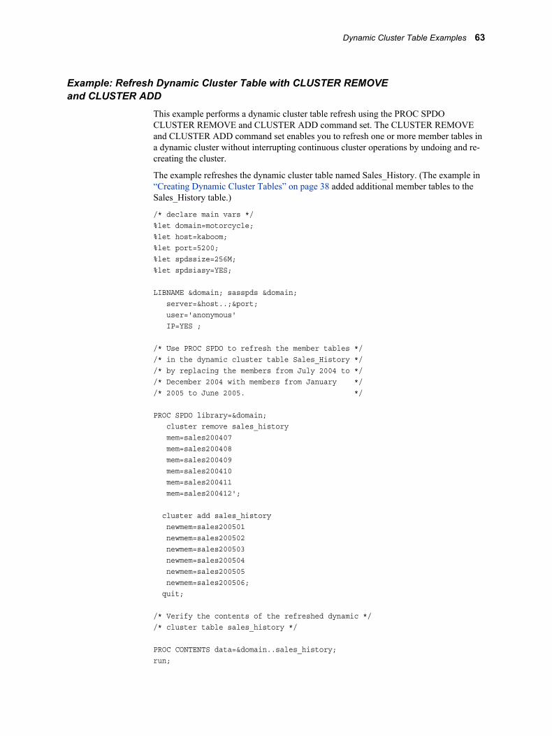
Example: Refresh Dynamic Cluster Table with CLUSTER REMOVE and CLUSTER ADD
This example performs a dynamic cluster table refresh using the PROC SPDO CLUSTER REMOVE and CLUSTER ADD command set. The CLUSTER REMOVE and CLUSTER ADD command set enables you to refresh one or more member tables in a dynamic cluster without interrupting continuous cluster operations by undoing and re-creating the cluster.
The example refreshes the dynamic cluster table named Sales_History. (The example in “Creating Dynamic Cluster Tables” on page 38 added additional member tables to the Sales_History table.)
/* declare main vars */%let domain=motorcycle;%let host=kaboom;%let port=5200;%let spdssize=256M;%let spdsiasy=YES;
LIBNAME &domain; sasspds &domain; server=&host..;&port; user='anonymous' IP=YES ;
/* Use PROC SPDO to refresh the member tables *//* in the dynamic cluster table Sales_History *//* by replacing the members from July 2004 to *//* December 2004 with members from January *//* 2005 to June 2005. */
PROC SPDO library=&domain; cluster remove sales_history mem=sales200407 mem=sales200408 mem=sales200409 mem=sales200410 mem=sales200411 mem=sales200412';
cluster add sales_history newmem=sales200501 newmem=sales200502 newmem=sales200503 newmem=sales200504 newmem=sales200505 newmem=sales200506; quit;
/* Verify the contents of the refreshed dynamic *//* cluster table sales_history */
PROC CONTENTS data=&domain..sales_history;run;
Dynamic Cluster Table Examples 63

Example: Undo and Refresh Dynamic Cluster TableThis example uses an older SPD Server method to refresh a dynamic cluster table by unbinding the cluster, changing the member tables, and then re-binding the cluster. This method remains functional, and can be used in SPD Server on SAS 9.4 and later. Most users will find the newer SPD Server commands for CLUSTER REMOVE / ADD and CLUSTER REPLACE produce identical results without requiring the dynamic cluster to be disassembled.
The example refreshes the dynamic cluster table named Sales_History. (The example in “Creating Dynamic Cluster Tables” on page 38 added additional member tables to the Sales_History table.) First, the 18-member dynamic cluster table Sales_History is unbound. The 12 member tables that contain 2004 sales data are deleted when the dynamic cluster table Sales_History is re-created. When the table is re-created, only the six member tables that contain 2005 sales data are included. These combined actions refresh the contents of the dynamic cluster table Sales_History.
/* declare main vars */%let domain=motorcycle;%let host=kaboom;%let port=5200;%let spdssize=256M;%let spdsiasy=YES;
LIBNAME &domain; sasspds &domain; server=&host..;&port; user='anonymous' IP=YES ;
/* Use PROC SPDO to undo the existing dynamic *//* cluster table Sales_History, then rebind *//* it with members from months in 2005 only */
PROC SPDO library=&domain; cluster undo sales_history; cluster create sales_history mem=sales200501 mem=sales200502 mem=sales200503 mem=sales200504 mem=sales200505 mem=sales200506; quit;
/* Verify the contents of the refreshed dynamic *//* cluster table sales_history */
PROC CONTENTS data=&domain..sales_history;run;
64 Chapter 6 • SAS Scalable Performance Data (SPD) Server Dynamic Cluster Tables
Part 3
SAS Scalable Performance Data (SPD) Server SQL Features
Chapter 7SAS Scalable Performance Data (SPD) Server SQL Features . . . . . . 67
65

66

Chapter 7
SAS Scalable Performance Data (SPD) Server SQL Features
Differences between SAS SQL and SPD Server SQL . . . . . . . . . . . . . . . . . . . . . . . . 69Reserved Keywords . . . . . . . . . . . . . . . . . . . . . . . . . . . . . . . . . . . . . . . . . . . . . . . . . 69Table Options and Delimiters . . . . . . . . . . . . . . . . . . . . . . . . . . . . . . . . . . . . . . . . . . 69Mixing Scalar Expressions and Boolean Predicates . . . . . . . . . . . . . . . . . . . . . . . . . 69INTO Clause . . . . . . . . . . . . . . . . . . . . . . . . . . . . . . . . . . . . . . . . . . . . . . . . . . . . . . . 69Tilde Negation . . . . . . . . . . . . . . . . . . . . . . . . . . . . . . . . . . . . . . . . . . . . . . . . . . . . . 69Nested Queries . . . . . . . . . . . . . . . . . . . . . . . . . . . . . . . . . . . . . . . . . . . . . . . . . . . . . 69USER Value . . . . . . . . . . . . . . . . . . . . . . . . . . . . . . . . . . . . . . . . . . . . . . . . . . . . . . . 70Supported Functions . . . . . . . . . . . . . . . . . . . . . . . . . . . . . . . . . . . . . . . . . . . . . . . . . 70
Connecting to the SPD Server SQL Engine . . . . . . . . . . . . . . . . . . . . . . . . . . . . . . . . 70Implicit Pass-Through Connection . . . . . . . . . . . . . . . . . . . . . . . . . . . . . . . . . . . . . . 70Explicit Pass-Through Connection . . . . . . . . . . . . . . . . . . . . . . . . . . . . . . . . . . . . . . 70LIBNAME Syntax to Specify a Libref . . . . . . . . . . . . . . . . . . . . . . . . . . . . . . . . . . . 70
Specifying SPD Server SQL Planner Options . . . . . . . . . . . . . . . . . . . . . . . . . . . . . . 71Specify SQL Options By Using Explicit Pass-Through Code . . . . . . . . . . . . . . . . . 71Specify SQL Options By Using Implicit Pass-Through Code . . . . . . . . . . . . . . . . . 72
Important SPD Server SQL Planner Options . . . . . . . . . . . . . . . . . . . . . . . . . . . . . . 72_method . . . . . . . . . . . . . . . . . . . . . . . . . . . . . . . . . . . . . . . . . . . . . . . . . . . . . . . . . . 72Reading the Method Tree . . . . . . . . . . . . . . . . . . . . . . . . . . . . . . . . . . . . . . . . . . . . . 73BUFFERSIZE= . . . . . . . . . . . . . . . . . . . . . . . . . . . . . . . . . . . . . . . . . . . . . . . . . . . . 74DETAILS= . . . . . . . . . . . . . . . . . . . . . . . . . . . . . . . . . . . . . . . . . . . . . . . . . . . . . . . . 74EXEC / NOEXEC . . . . . . . . . . . . . . . . . . . . . . . . . . . . . . . . . . . . . . . . . . . . . . . . . . . 75HASHINSETSIZE . . . . . . . . . . . . . . . . . . . . . . . . . . . . . . . . . . . . . . . . . . . . . . . . . . 75INDEXSELECTIVITY= . . . . . . . . . . . . . . . . . . . . . . . . . . . . . . . . . . . . . . . . . . . . . 75INOBS . . . . . . . . . . . . . . . . . . . . . . . . . . . . . . . . . . . . . . . . . . . . . . . . . . . . . . . . . . . 76JTECH PREF | JOINTECH_PREF . . . . . . . . . . . . . . . . . . . . . . . . . . . . . . . . . . . . . 77MAXHASHJOIN . . . . . . . . . . . . . . . . . . . . . . . . . . . . . . . . . . . . . . . . . . . . . . . . . . . 77OUTOBS . . . . . . . . . . . . . . . . . . . . . . . . . . . . . . . . . . . . . . . . . . . . . . . . . . . . . . . . . 77OUTRSRTJNDX / NOOUTRSRTJNDX . . . . . . . . . . . . . . . . . . . . . . . . . . . . . . . . . 78PRINTLOG / NOPRINTLOG . . . . . . . . . . . . . . . . . . . . . . . . . . . . . . . . . . . . . . . . . 78SASVIEW / NOSASVIEW . . . . . . . . . . . . . . . . . . . . . . . . . . . . . . . . . . . . . . . . . . . 78UNDO_POLICY= . . . . . . . . . . . . . . . . . . . . . . . . . . . . . . . . . . . . . . . . . . . . . . . . . . 79Additional SQL Reset Options . . . . . . . . . . . . . . . . . . . . . . . . . . . . . . . . . . . . . . . . . 80
Parallel Join Facility . . . . . . . . . . . . . . . . . . . . . . . . . . . . . . . . . . . . . . . . . . . . . . . . . . . 80Overview of the Parallel Join Facility . . . . . . . . . . . . . . . . . . . . . . . . . . . . . . . . . . . 80Criteria for Using the Parallel Join Facility . . . . . . . . . . . . . . . . . . . . . . . . . . . . . . . 80Parallel Join Methods . . . . . . . . . . . . . . . . . . . . . . . . . . . . . . . . . . . . . . . . . . . . . . . . 80Parallel Joins with Group-By . . . . . . . . . . . . . . . . . . . . . . . . . . . . . . . . . . . . . . . . . . 81Parallel Join SQL Options . . . . . . . . . . . . . . . . . . . . . . . . . . . . . . . . . . . . . . . . . . . . 82
67

Parallel Join Example 1 . . . . . . . . . . . . . . . . . . . . . . . . . . . . . . . . . . . . . . . . . . . . . . 82Parallel Join Example 2 . . . . . . . . . . . . . . . . . . . . . . . . . . . . . . . . . . . . . . . . . . . . . . 83Parallel Join Example 3 . . . . . . . . . . . . . . . . . . . . . . . . . . . . . . . . . . . . . . . . . . . . . . 83
Parallel Group-By Facility . . . . . . . . . . . . . . . . . . . . . . . . . . . . . . . . . . . . . . . . . . . . . . 83Overview of the Parallel Group-By Facility . . . . . . . . . . . . . . . . . . . . . . . . . . . . . . . 83Enhanced Group-By Functions . . . . . . . . . . . . . . . . . . . . . . . . . . . . . . . . . . . . . . . . . 84Nested Queries Meet Group-By Syntax Requirements . . . . . . . . . . . . . . . . . . . . . . 84Formatted Parallel Group Select . . . . . . . . . . . . . . . . . . . . . . . . . . . . . . . . . . . . . . . . 85
Parallel Group-By SQL Reset Options . . . . . . . . . . . . . . . . . . . . . . . . . . . . . . . . . . . . 87GRPSEL / NOGRPSEL . . . . . . . . . . . . . . . . . . . . . . . . . . . . . . . . . . . . . . . . . . . . . . 87FMTGRPSEL / NOFMTGRPSEL . . . . . . . . . . . . . . . . . . . . . . . . . . . . . . . . . . . . . . 88SCANGRPSEL / NOSCANGRPSEL . . . . . . . . . . . . . . . . . . . . . . . . . . . . . . . . . . . 88
SPD Server STARJOIN Facility . . . . . . . . . . . . . . . . . . . . . . . . . . . . . . . . . . . . . . . . . 88Overview of the SPD Server STARJOIN Facility . . . . . . . . . . . . . . . . . . . . . . . . . . 88Star Schemas . . . . . . . . . . . . . . . . . . . . . . . . . . . . . . . . . . . . . . . . . . . . . . . . . . . . . . . 89SPD Server STARJOIN Requirements . . . . . . . . . . . . . . . . . . . . . . . . . . . . . . . . . . 90Invoking the SPD Server STARJOIN Facility . . . . . . . . . . . . . . . . . . . . . . . . . . . . . 90Indexing Strategies to Optimize STARJOIN Query Performance . . . . . . . . . . . . . . 91
STARJOIN RESET Statement Options . . . . . . . . . . . . . . . . . . . . . . . . . . . . . . . . . . . 93Overview of STARJOIN Reset Statement Options . . . . . . . . . . . . . . . . . . . . . . . . . 93RESET NOSTARJOIN=[0/1] . . . . . . . . . . . . . . . . . . . . . . . . . . . . . . . . . . . . . . . . . 93RESET STARMAGIC=nnn . . . . . . . . . . . . . . . . . . . . . . . . . . . . . . . . . . . . . . . . . . . 94RESET DETAILS="stj$" . . . . . . . . . . . . . . . . . . . . . . . . . . . . . . . . . . . . . . . . . . . . . 94Example: STARJOIN RESET Statements . . . . . . . . . . . . . . . . . . . . . . . . . . . . . . . . 94
SPD Server STARJOIN Examples . . . . . . . . . . . . . . . . . . . . . . . . . . . . . . . . . . . . . . . 95Example 1: Valid SQL STARJOIN Candidate . . . . . . . . . . . . . . . . . . . . . . . . . . . . 95Example 2: Invalid SQL STARJOIN Candidate . . . . . . . . . . . . . . . . . . . . . . . . . . . 96Example 3: STARJOIN Candidate with Created or Calculated Columns . . . . . . . . 96
SPD Server Join Planner . . . . . . . . . . . . . . . . . . . . . . . . . . . . . . . . . . . . . . . . . . . . . . . 97
SPD Server Index Scan . . . . . . . . . . . . . . . . . . . . . . . . . . . . . . . . . . . . . . . . . . . . . . . . 97
Optimizing Correlated Queries . . . . . . . . . . . . . . . . . . . . . . . . . . . . . . . . . . . . . . . . . 100
Correlated Query Options . . . . . . . . . . . . . . . . . . . . . . . . . . . . . . . . . . . . . . . . . . . . . 100_QRW / NO_QRW . . . . . . . . . . . . . . . . . . . . . . . . . . . . . . . . . . . . . . . . . . . . . . . . . 100_QRWENABLE / NO_QRWENABLE . . . . . . . . . . . . . . . . . . . . . . . . . . . . . . . . . 101
SPD Server SQL Views . . . . . . . . . . . . . . . . . . . . . . . . . . . . . . . . . . . . . . . . . . . . . . . 102Overview of SPD Server SQL Views . . . . . . . . . . . . . . . . . . . . . . . . . . . . . . . . . . . 102View Access Inheritance . . . . . . . . . . . . . . . . . . . . . . . . . . . . . . . . . . . . . . . . . . . . 102Materialized Views . . . . . . . . . . . . . . . . . . . . . . . . . . . . . . . . . . . . . . . . . . . . . . . . . 103
SPD Server SQL Extensions . . . . . . . . . . . . . . . . . . . . . . . . . . . . . . . . . . . . . . . . . . . 106BEGIN and END ASYNC OPERATION Statements . . . . . . . . . . . . . . . . . . . . . . 106LOAD Statement . . . . . . . . . . . . . . . . . . . . . . . . . . . . . . . . . . . . . . . . . . . . . . . . . . 110COPY Statement . . . . . . . . . . . . . . . . . . . . . . . . . . . . . . . . . . . . . . . . . . . . . . . . . . . 112
SPD Server SQL Cluster Operations . . . . . . . . . . . . . . . . . . . . . . . . . . . . . . . . . . . . 113CLUSTER CREATE . . . . . . . . . . . . . . . . . . . . . . . . . . . . . . . . . . . . . . . . . . . . . . . 113CLUSTER UNDO . . . . . . . . . . . . . . . . . . . . . . . . . . . . . . . . . . . . . . . . . . . . . . . . . 113CLUSTER REMOVE and CLUSTER ADD . . . . . . . . . . . . . . . . . . . . . . . . . . . . . 114CLUSTER REPLACE . . . . . . . . . . . . . . . . . . . . . . . . . . . . . . . . . . . . . . . . . . . . . . 114
68 Chapter 7 • SAS Scalable Performance Data (SPD) Server SQL Features
Differences between SAS SQL and SPD Server SQL
Reserved KeywordsSPD Server uses keywords to initiate statements or to refer to syntax elements. For example, you can use the words where and group only in certain ways because SPD Server uses WHERE and GROUP BY clauses. Keywords are treated as reserved words. You cannot use keywords in the name of a libref, a table, a column, or an index.
In contrast, SAS SQL allows keywords in some, but not all, syntax locations. For more information about keywords that are restricted by SPD Server, see “Reserved Keywords” on page 308 .
Table Options and DelimitersSPD Server SQL uses brackets to delimit table options. SAS SQL uses parentheses as delimiters. You can place table options in a CREATE TABLE statement. You must put table options inside parentheses to delimit column definitions in a table.
Mixing Scalar Expressions and Boolean PredicatesSPD Server SQL does not allow mixing scalar expressions with Boolean predicates. SAS SQL does allow mixing scalar expressions with Boolean predicates in most places. For more information about what content is permissible in expressions, see “Scalar Expressions and Boolean Predicates” on page 307 .
INTO ClauseSPD Server SQL does not support the INTO clause. For example, SPD Server SQL does not support the following statement:
select a, b into :var1, :var2 from t where a > 7;
In contrast, SAS SQL supports the INTO clause.
Tilde NegationSPD Server SQL supports the use of the tilde character (~) only to negate the equals operator (=), as in ~= (not equals). SAS SQL supports the use of the tilde character where the tilde is synonymous with not and can be combined with various operators. For example, SAS SQL can use the tilde with the BETWEEN operator, as in ~BETWEEN (not between). SPD Server does not recognize this expression.
Nested QueriesSAS SQL permits subqueries without delimiting parentheses in more places than does SPD Server SQL. SPD Server SQL uses parentheses to explicitly group subqueries or expressions that are nested in a query statement whenever possible. Queries with nested expressions execute more reliably and are also easier to read.
Differences between SAS SQL and SPD Server SQL 69
USER ValueSPD Server SQL does not support the USER keyword in the INSERT statement. For example, the following query fails in SPD Server SQL:
insert into t1(myname) values(USER);
Supported FunctionsSPD Server SQL does not support all of the SQL functions that SAS supports. For a complete list of the SQL functions that SPD Server SQL supports, see “SQL Functions Supported by SPD Server” on page 319.
For a complete list of the SQL WHERE processing functions that SPD Server SQL supports, see “SQL WHERE-Processing Functions Supported by SPD Server” on page 320.
Connecting to the SPD Server SQL Engine
Implicit Pass-Through ConnectionYou can use an implicit pass-through connection to pass implicit SQL statements to the SPD Server SQL engine. When you use an implicit pass-through connection, the SAS SQL Planner parses SQL statements to determine which, if any, portions can be passed to the SPD Server SQL engine. In order for a submitted SQL statement to take advantage of implicit pass-through SQL, the tables that are referenced in the SQL statement must be SPD Server tables, and the SPD Server SQL engine must be able to successfully parse the submitted SQL statement. If SPD Server cannot successfully parse the statement, an SPD Server parse error is reported in the SAS log, and SAS SQL retries the query.
For an example of an SPD Server implicit pass-through connection, see “Specify SQL Options By Using Implicit Pass-Through Code” on page 72.
Explicit Pass-Through ConnectionYou can use an explicit pass-through connection to pass explicit SQL statements to the SPD Server SQL engine. When you use an explicit pass-through connection, you decide explicitly which SQL statements are passed to the SPD Server SQL engine. The explicit pass-through connection passes the entire SQL statement as written to the SPD Server SQL engine, which parses and plans the SQL statement. All tables that are referenced in the SQL statement must be SPD Server tables or an error occurs.
For an example of an SPD Server explicit pass-through connection, see “Specify SQL Options By Using Explicit Pass-Through Code” on page 71.
LIBNAME Syntax to Specify a LibrefThe following LIBNAME statement associates a libref, the SASSPDS engine, and an SPD Server domain.
LIBNAME libref
70 Chapter 7 • SAS Scalable Performance Data (SPD) Server SQL Features
SASSPDS <'SAS-data-library'> <SPD Server-options>;
Use the following arguments:
librefa name that is up to 8 characters long and that conforms to the rules for SAS names.
SASSPDSthe name of the SPD Server engine.
'SAS-data-library'the logical LIBNAME domain name for an SPD Server data library on the host machine. The name server resolves the domain name to the physical path for the library.
SPD Server-optionsone or more SPD Server options.
Specifying SPD Server SQL Planner OptionsThe SPD Server SQL language provides reset options that you can use to configure the behavior of the SQL language. You can also use these options to configure the SPD Server facilities that function through the SQL Planner, such as the SPD Server Parallel Group-By facility, the SPD Server Parallel Join facility, and the SPD Server STARJOIN facility. You can specify SPD Server SQL reset options by using either explicit pass-through or implicit pass-through code.
Specify SQL Options By Using Explicit Pass-Through CodeThe following example shows how to use an execute(reset <reset-options>) statement in explicit SPD Server pass-through SQL code to invoke an SQL Planner, Parallel Group-By facility, Parallel Join facility, or STARJOIN facility reset option.
Most usage examples of the SQL Planner reset option in this document use explicit pass-through code. For an example of how you can declare SQL reset options by using an implicit %let spdssqlr= statement instead of an explicit execute(reset <reset-options>) statement, see “Specify SQL Options By Using Implicit Pass-Through Code” on page 72.
/* Explicit Pass-Through SQL Example *//* to invoke an SQL Reset Option */
PROC SQL ;
connect to sasspds ( dbq='MyDomainName' server='NameServerID'.'NameServerPortNumber' user='wnelson') ;
execute(reset PRINTLOG) by sasspds ;
execute(SQL statements) by sasspds ;
disconnect from sasspds ;
Specifying SPD Server SQL Planner Options 71
quit ;
Specify SQL Options By Using Implicit Pass-Through CodeThe following example shows how to use a %let spdssqlr=<reset-options> statement in implicit SPD Server pass-through SQL code to invoke an SQL Planner, Parallel Group-By facility, Parallel Join facility, or STARJOIN facility reset option.
Most usage examples of the SQL Planner reset option in this document use explicit pass-through code. The following implicit pass-through code example shows how you can declare SQL reset options by using an implicit %let spdssqlr= statement instead of an explicit execute(reset <reset-options>) statement.
/* Implicit Pass-Through SQL Example *//* to invoke an SQL Reset Option */
%let spdssqlr= INOBS=1000 ;
PROC SQL ;SQL statements ;
quit ;
Important SPD Server SQL Planner Options
_methodThe SQL _method option is one of the most important reset options. The _method reset option provides a method tree in the output that shows how the SQL was planned and executed.
The following methods are displayed in the SQL _method tree:
sqxcrtaCreate table as Select.
sqxslctSelect rows from table.
sqxjslStep loop join (Cartesian join).
sqxjmMerge join execution.
sqxjndxIndex join execution.
sqxjhshHash join execution.
sqxsortSort table or rows.
sqxsrcRead rows from source.
72 Chapter 7 • SAS Scalable Performance Data (SPD) Server SQL Features
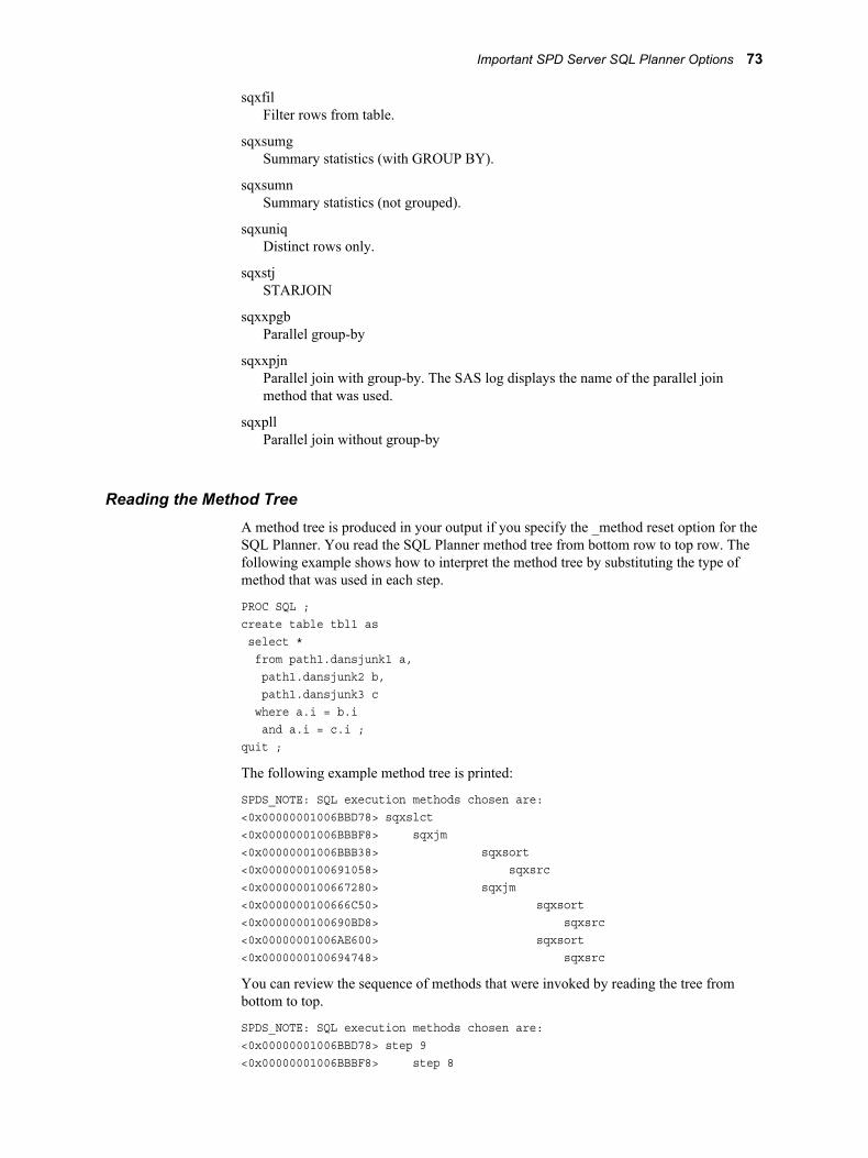
sqxfilFilter rows from table.
sqxsumgSummary statistics (with GROUP BY).
sqxsumnSummary statistics (not grouped).
sqxuniqDistinct rows only.
sqxstjSTARJOIN
sqxxpgbParallel group-by
sqxxpjnParallel join with group-by. The SAS log displays the name of the parallel join method that was used.
sqxpllParallel join without group-by
Reading the Method TreeA method tree is produced in your output if you specify the _method reset option for the SQL Planner. You read the SQL Planner method tree from bottom row to top row. The following example shows how to interpret the method tree by substituting the type of method that was used in each step.
PROC SQL ;create table tbl1 as select * from path1.dansjunk1 a, path1.dansjunk2 b, path1.dansjunk3 c where a.i = b.i and a.i = c.i ;quit ;
The following example method tree is printed:
SPDS_NOTE: SQL execution methods chosen are:<0x00000001006BBD78> sqxslct<0x00000001006BBBF8> sqxjm<0x00000001006BBB38> sqxsort<0x0000000100691058> sqxsrc<0x0000000100667280> sqxjm<0x0000000100666C50> sqxsort<0x0000000100690BD8> sqxsrc<0x00000001006AE600> sqxsort<0x0000000100694748> sqxsrc
You can review the sequence of methods that were invoked by reading the tree from bottom to top.
SPDS_NOTE: SQL execution methods chosen are:<0x00000001006BBD78> step 9<0x00000001006BBBF8> step 8
Important SPD Server SQL Planner Options 73

<0x00000001006BBB38> step 7<0x0000000100691058> step 6<0x0000000100667280> step 5<0x0000000100666C50> step 4<0x0000000100690BD8> step 3<0x00000001006AE600> step 2<0x0000000100694748> step 1
In step 1, sqxsrc reads rows from the source. In step 2, sqxsort sorts the table rows. Then in steps 3 and 4, more rows are read and sorted. In step 5, the tables are joined by sqxjm, and so on.
BUFFERSIZE=The SPD Server query optimizer considers a number of join strategies. Some of the join strategies require memory buffers. In these cases, BUFFERSIZE= specifies the amount of memory that SPD Server should reserve for memory buffers.
For example, SPD Server SQL might consider a hash join when an index join is not possible. A hash join reconfigures the smaller table in memory as a hash table. SQL sequentially scans the larger table and performs a hash lookup row-by-row against the smaller table to form the result set. On a memory-rich system, consider increasing the BUFFERSIZE= option to increase the likelihood that a hash join is chosen. The default BUFFERSIZE= setting is 64 K. You can specify the amount of memory that you want SPD Server to use for hash joins.
Usage:
/* Increase buffersize from 64K */execute(reset buffersize=n)by sasspds ;
nthe maximum number of rows in the smaller table for a hash join that can use the inset size hash join optimization.
DETAILS=Use the DETAILS= reset switch to provide additional information in the SAS log about the SQL joins that SPD Server made.
Usage:
execute(reset details=("what_join$"|"why_join$"|"what_join$why_join$") by sasspds ;
DETAILS="what_join$"adds additional information in the SAS log documenting the join plan that was selected.
DETAILS="why_join$"adds additional information in the SAS log documenting why the join plan that was selected was chosen.
74 Chapter 7 • SAS Scalable Performance Data (SPD) Server SQL Features

DETAILS="what_why_join$"adds additional information in the SAS log documenting the join plan that was selected, and why the join plan that was selected was chosen.
EXEC / NOEXECYou use the SPD Server SQL Planner EXEC / NOEXEC option to turn SPD Server SQL execution on or off.
Usage:
/* This explicit Pass-Through SQL *//* prints the method tree without *//* executing the SQL code. */
PROC SQL ;connect to sasspds (dbq=domain server=<host-name>.<port-number> user='username') ;
execute (reset _method noexec) by sasspds ; /* turns SQL exec off */
execute (SQL statements) by sasspds ;
disconnect from sasspds ;quit ;
HASHINSETSIZEYou use the SPD Server SQL planner HASHINSETSIZE reset option to influence when the hash join inset size optimization can be used. The hash join inset size optimization gathers join keys from the smaller join table, and then generates a query to the larger table. The query to the larger table only selects rows that can be joined to the smaller table. that only selects rows that can be joined to the smaller table. The join keys for the selected rows of the larger table are then hashed with the smaller table in order to perform the hash join.
Usage:
execute(reset hashinsetsize=nby sasspds;
nthe maximum number of rows in the smaller table for a hash join that can use the inset size hash join optimization.
INDEXSELECTIVITY=The INDEXSELECTIVITY= option enables you to tune the SQL join planner strategy for more efficient or robust index join methods. The INDEXSELECTIVITY= setting is a continuous value in the range 0–1 that acts as a minimum threshold value for the SPD Server cardinality ratio when selecting a join method. The SPD Server cardinality ratio
Important SPD Server SQL Planner Options 75
is a heuristic that acts as a measure of the cardinality of the inner table index, relative to the frequency of index values as they occur in the outer table. Both INDEXSELECTIVITY= and the SPD Server cardinality ratio are continuous values between 0 and 1. SPD Server compares the calculated cardinality ratio for an SPD Server index join to the value that you specify in the INDEXSELECTIVITY= option. If the calculated cardinality ratio is greater than or equal to the value that is specified in the INDEXSELECTIVITY= option, SPD server chooses the index join method. The default setting for the INDEXSELECTIVITY= option is 0.7.
How does SPD Server calculate the cardinality ratio? The cardinality ratio of an indexed column is calculated as the number of unique values in the index column, divided by the number of rows in the outer table. As the value of the cardinality ratio approaches 0, which indicates low cardinality, the greater the number of duplicate values that exist in the rows of the outer table. As the value of the cardinality ratio approaches 1, which indicates high cardinality, the fewer the number of duplicate index values in the rows of the outer table. For example, a cardinality ratio of 1/1, or 1, represents a unique index value for every row in the outer table, a unique index. A cardinality ratio value of 1/2, or 0.5, represents a unique index value for every two rows in the outer table. A cardinality ratio value of 1/4, or 0.25, represents a unique index value for every four rows in the outer table. The default setting of INDEXSELECTIVITY= is 0.7, which represents a unique index value for every 1.43 rows in the outer table.
For example, consider an outer table that contains 100 rows that match join key values in the inner table, and a calculated SPD Server cardinality ratio of 0.7 (a unique index value per 1.43 rows in the outer table). The expected result set is 100*1.43, or 143 rows.
Higher cardinality and higher index cardinality ratios are associated with an efficient index join. Cardinality ratios near 1 result in more efficient processing during probes between the outer table rows and the inner table index, because each probe has fewer rows to retrieve. In turn, the work that the SPD Server index must do to find and retrieve the matching rows during the join operation is maximized, which results in an optimized index join.
You can use INDEXSELECTIVITY= to configure the index join to be more or less tightly constrained by the number of duplicate values in the join table rows. Increasing the value of INDEXSELECTIVITY= makes the cardinality criteria more selective by decreasing the allowable average number of rows per probe of the inner table. Setting INDEXSELECTIVITY= equal to 1.0 allows only a join with a unique index. Setting INDEXSELECTIVITY= to a value greater than 1.0 allows no index joins. Decreasing the value of INDEXSELECTIVITY= makes the cardinality criteria more flexible by increasing the allowable average number of rows per probe of the inner table. Setting INDEXSELECTIVITY= equal to 0.0 allows joins with any amount of cardinality.
Usage:
execute(reset indexselectivity=<0.0 ... 1.0>) by sasspds ;
INOBSUse the INOBS option to specify the specific number of observations that you want to read from input tables.
Usage:
execute(reset inobs=<n>) by sasspds ;
The integer value <n> is the number of observations that you want to read.
76 Chapter 7 • SAS Scalable Performance Data (SPD) Server SQL Features
JTECH PREF | JOINTECH_PREFYou use the SPD Server SQL Planner JTECH PREF | JOINTECH_PREF reset option to control how the SPD Server SQL Planner executes join statements. The option has three settings: 101, 102, and 103.
Usage:
execute(reset jointech_pref=<seq|merge|hash|index>) by sasspds ;
where
JOINTECH_PREF=seqSPD Server performs sequential loop joins. Sequential loop joins are brute force joins that match every row of the first table to every row of the second table.
JOINTECH_PREF=mergeSPD Server performs sort merge joins. Sort merge joins force a sort on all tables that are involved in the join.
JOINTECH_PREF=hashSPD Server performs hash joins. Hash joins require SPD Server to create a memory table in order to perform the join. The size of the memory table is limited based on the available memory.
JOINTECH_PREF=indexSPD server will favor an index join, provided the join meets the index join criteria. The index join requires an index on the join column of one tables, and the index_selectivity requirement must be met (see the index_selectivity reset option).
MAXHASHJOINYou use the SPD Server SQL planner MAXHASHJOIN reset option to control how many hash joins can be planned in a single statement.
Usage:
execute(reset maxhashjoins=<n>)by sasspds;
nthe number of hash joins that can be planned.
Note: Hash joins in SPD Server can be memory intensive. Increasing the number of hash joins is likely to increase the memory requirements for the query plan.
OUTOBSUse the OUTOBS option to specify the specific number of observations that you want to create or print in your output.
Usage:
execute(reset outobs=<n>) by sasspds ;
Important SPD Server SQL Planner Options 77
The integer value <n>is the number of observations that you want to create or print.
OUTRSRTJNDX / NOOUTRSRTJNDXUse the OUTRSRTJNDX / NOOUTRSRTJNDX option to configure the sort behavior for an SPD Server join index. OUTRSRTJNDX sorts the outer table for a join index by the join key. This setting is the default SPD Server setting. NOOUTRSRTJNDX does not sort the outer table for a join index.
Usage:
/* Disable outer table *//* sorting for a join index */execute(reset nooutrsrtjndx) by sasspds ;
/* Enable outer table *//* sorting for a join index */execute(reset outrsrtjndx) by sasspds ;
PRINTLOG / NOPRINTLOGYou use the PRINTLOG / NOPRINTLOG option of the SPD Server SQL Planner to turn on or off the printing of the SQL statement text to the SPD Server log.
Usage:
PROC SQL ;connect to sasspds (dbq=domain server=<host-name>.<port-number> user='username') ;
/* turn SQL statement printing on */execute (reset printlog)by sasspds ;
/* all statements will be printed to SPD Server log */execute (SQL statements)by sasspds ;
/* turn SQL statement printing off */execute (reset noprintlog)by sasspds ;
disconnect from sasspds ;quit ;
SASVIEW / NOSASVIEWUse the SASVIEW / NOSASVIEW option to enable or disable SAS PROC SQL views that use an SPD Server LIBNAME. SAS PROC SQL views use a generic transport format to represent numeric values, which SPD Server converts to native numeric
78 Chapter 7 • SAS Scalable Performance Data (SPD) Server SQL Features

values. When extremely large or extremely small numeric values are conveyed in a SAS PROC SQL view to SPD Server, extreme values might not be as precise during the SPD Server numeric conversion.
Usage:
/* Disable SAS PROC SQL views *//* that use an SPD Server LIBNAME */execute(reset nosasview) by sasspds ;
/* Enable SAS PROC SQL views that *//* use an SPD Server LIBNAME */execute(reset sasview) by sasspds ;
If SAS PROC SQL views are disabled and SPD Server pass-through SQL uses a view that was created by PROC SQL, SPD Server rejects the PROC SQL statement and inserts the following error message in the SAS log:
SPDS_WARNING: SAS View and SASVIEW Reset Option equals No.SPDS_ERROR: An error has occured.
If SAS PROC SQL views are enabled and SPD Server pass-through SQL uses a view that was created by PROC SQL, SPD Server prints the following note in the SAS log:
SPDS_NOTE: SPDS using SAS View in transport mode.
UNDO_POLICY=Use the UNDO_POLICY option in SPD Server PROC SQL and RESET statements to configure SPD Server PROC SQL error recovery. When you update or insert rows in a table, you might receive an error message that states that the Update or Insert operation cannot be performed. The UNDO_POLICY option specifies how you want SPD Server to handle rows that were affected by INSERT or UPDATE statements that preceded a processing error.
Usage:
/* Do not undo any updates or inserts */execute(reset undo_policy=none) by sasspds ;
/* Permit row inserts and updates to *//* be done up to the point of error */execute(reset undo_policy=required) by sasspds ;
UNDO_POLICY=NONEthe default setting for SPD Server. This setting does not undo any updates or inserts.
UNDO_POLICY=REQUIREDundoes all row updates or inserts up to the point of error.
UNDO_POLICY=OPTIONALundoes any updates or inserts that it can undo reliably.
If the UNDO policy is not required, you get the following warning message for an insert into the table:
WARNING: The SQL option UNDO_POLICY=REQUIRED is not in effect. If an
Important SPD Server SQL Planner Options 79

error is detected when processing this insert statement, that errorwill not cause the entire statement to fail.
Additional SQL Reset OptionsFor more detailed information about the available SQL reset options for the SPD Server SQL Parallel Join, Parallel Group-By, STARJOIN, and Correlated Query facilities, see the following topics:
• “Parallel Join SQL Options” on page 82
• “Parallel Group-By SQL Reset Options” on page 87
• “STARJOIN RESET Statement Options” on page 93
• “Correlated Query Options” on page 100
Parallel Join Facility
Overview of the Parallel Join FacilityThe Parallel Join facility is a feature of the SPD Server SQL Planner that decreases the processing time that is required to create a pairwise join between two SPD Server tables. The savings in processing time is created when SPD Server performs the pairwise join in parallel.
The SQL Planner first searches for pairs when SPD Server source tables are to be joined. When the Planner finds a pair, it checks the join syntax for that pair to determine whether the syntax meets all of the requirements for the Parallel Join facility. If the join syntax meets the requirements, the pair of tables are joined by the Parallel Join facility.
Criteria for Using the Parallel Join FacilityThe criteria for using the SPD Server Parallel Join facility can be more complex than simply requiring a pairwise join of two SPD Server tables. The Parallel Join facility can handle multiple character columns, numeric columns, or combinations of character and numeric columns that are joined between pairs of tables. Numeric columns do not need to be of the same width to act as a join key, but character columns must be of the same width in order to be a join key. Columns that are involved in a join cannot be derived from a SAS CASE statement, and cannot be created from character manipulation functions such as SUBSTR, YEAR, MONT, DAY, and TRIM.
Parallel Join Methods
Parallel Sort-Merge MethodThe parallel sort-merge join method first performs a parallel sort to order the data, and then merges the sorted tables in parallel. During the merge, the facility concurrently joins multiple rows from one table with the corresponding rows in the other table. You can use the parallel sort-merge join method to execute any join that meets the requirements for a parallel join.
80 Chapter 7 • SAS Scalable Performance Data (SPD) Server SQL Features

The parallel sort-merge method is a good, all-around parallel join strategy that requires no intervention from you. The tables for the sort-merge method do not need to be in the same domain. The sort-merge method is not affected by the distribution of the data in the sort key columns.
The sort-merge method begins by completely sorting the smaller of the two tables that are being joined, while simultaneously performing partial parallel sorts on the larger table. If both tables are very large and sufficient resources are not available to do the complete sort on the smaller table, the performance of the parallel sort-merge method can degrade. The parallel sort-merge method is also limited when you are performing an outer, left, or right join in parallel. Parallel outer, left, or right joins can use only two concurrent threads. Inner joins are not limited in the parallel sort-merge method and can use more than two concurrent threads during parallel operations.
Parallel Range Join MethodThe parallel range join method uses a join index to determine the ranges of rows between the tables that can be joined in parallel. The parallel range join method requires you to create a join index on the columns to be joined in the tables that you want to merge. The join index divides the two tables into a specified number of near-equal parts, or ranges, based on matching values between the join columns. The Parallel Join facility recognizes the ranges of rows that contain matching values between the join columns, and then uses concurrent join threads to join the rows in parallel. The SPD Server parallel sort then sorts the rows within a range.
You can use the parallel range join method only on tables that are in the same domain. If either of the two tables are updated after the join index is created, you must rebuild the join index before you can use the parallel range join method. The parallel range join method performs best when the columns of the tables that are being joined are sorted. If the columns are not relatively sorted, then the concurrent join threads can cause processor thrashing. Processor thrashing occurs when unsorted rows in a table require SPD Server to perform increasingly larger table row scans, which can consume processor resources at a high rate during concurrent join operations.
For more information about creating join indexes, see Chapter 22, “SAS Scalable Performance Data (SPD) Server Index Utility Ixutil ,” in SAS Scalable Performance Data Server: Administrator's Guide.
How does the SPD Server Parallel Join facility choose between the sort-merge method and the range join method? If a join index is available for the tables to be joined, the Parallel Join facility chooses the parallel range join method. If a join index does not exist, or if the join index has not been rebuilt because a table was updated, the Parallel Join facility defaults to using the parallel sort-merge method.
Parallel Joins with Group-ByA powerful feature of the SPD Server Parallel Join facility is its integration with the SPD Server Parallel Group-By facility. If the result of the parallel join contains a GROUP BY statement, the partial results of the parallel join threads are passed to the Parallel Group-By facility, which performs the group-by operation in parallel. In the following example, SPD Server performs both a parallel join and parallel group-by operation.
LIBNAME path1 sasspds .... IP=YES;
PROC SQL;create table junk as select a.c, b.d, sum(b.e) from path1.table1 a,
Parallel Join Facility 81

path1.table2 b where a.i = b.i group by a.d, b.d;quit;
When you use the SPD Server Parallel Join facility, you can use the parallel group-by method on multiple tables.
Parallel Join SQL Options
PLLJOIN / NOPLLJOINThe PLLJOIN / NOPLLJOIN option enables and disables the SPD Server Parallel Join facility.
Usage:
execute(reset noplljoin) by sasspds ; /* disables Parallel Join */
CONCURRENCY=The CONCURRENCY=<n> option sets the concurrency level that the SPD Server Parallel Join facility uses. The integer value n specifies the number of levels. In most cases, you should not change the default SPD Server concurrency setting, which is half of the available number of processors.
Usage:
execute(reset concurrency=4) by sasspds ; /* enables 4 concurrency levels */
PLLJMAGICThe PLLJMAGIC option specifies how SPD server performs parallel joins.
Usage:
execute(reset plljmagic=<100/200>) by sasspds ;
PLLJMAGIC=100 forces a parallel range join when the range index is available.
PLLJMAGIC=200 forces a parallel merge join.
Parallel Join Example 1The example is a basic SQL query that creates a pairwise join of two SPD Server tables, table1 and table2.
LIBNAME path1 sasspds .... IP=YES;
PROC SQL;create table junk as select * from path1.table1 a, path1.table2 b where a.i = b.i; quit;
82 Chapter 7 • SAS Scalable Performance Data (SPD) Server SQL Features
Parallel Join Example 2This example is an SQL query that uses more than two SPD Server tables. The SQL Planner performs a parallel join on table1 and table2, and then use a non-parallel method to join the results of the first join and table3. The second join uses a non-parallel join method because the criteria for a parallel join were not met. A parallel join can be performed only on a pairwise join of two SPD Server tables and the query calls three SPD Server tables.
LIBNAME path1 sasspds .... IP=YES;
PROC SQL;create table junk as select * from path1.table1 a, path1.table2 b, path1.table3 c where a.i = b.i and b.i = c.i;quit;
Parallel Join Example 3You can use multiple parallel joins in the same SQL query, as long as the SQL Planner can perform the query by using more than one pairwise join. In this parallel join example, a more complex query contains a union of two separate joins. Both joins are pairwise joins of two SPD Server tables. There is a pairwise join between table1 and table2. A pairwise join between table3 and table4 is performed concurrently, using the Parallel Join facility.
PROC SQL;create table junk as select * from path1.table1 a, path1.table2 b where a.i = b.i union
select * from path1.table3 c,path1.table4 dwhere c.i = d.i;quit;
Parallel Group-By Facility
Overview of the Parallel Group-By FacilitySPD Server SQL Planner optimizations improve the performance of the more frequent query types used in data mining solutions. One of the SQL Planner optimizations is the Parallel Group-By capability. Parallel Group-By is a high-performance parallel summarization of data that is executed using SQL. Parallel Group-By is often used in
Parallel Group-By Facility 83
SQL queries (through the use of sub queries) to apply selection lists for inclusion or exclusion. The tighter integration adds performance benefits to nested Group-By syntax.
Parallel Group-By looks for specific patterns in a query that can be performed by using parallel processing summarization. Parallel Group-By works against single tables that are used to aggregate data. Parallel processing summarization is limited to the types of functions that it can handle.
The Parallel Group-By support in SPD Server is integrated into the WHERE clause planner code so that it boosts the capabilities of the SPD Server SQL engine. Any section of code that matches the Parallel Group-By trigger pattern will use Parallel Group-By support.
Enhanced Group-By FunctionsParallel Group-By supports the following functions in syntax: COUNT, FREQ, N, USS, CSS, AVG, MEAN, MAX, MIN, NMISS, RANGE, STD, STDERR, SUM, VAR. All these functions can accept the DISTINCT term. These functions are the minimum summary functions that are required in order to support the SAS Marketing Automation tool suite.
Nested Queries Meet Group-By Syntax RequirementsBecause the Parallel Group-By functionality is integrated into the SPD Server WHERE clause planner, many sections of queries can take advantage of performance enhancements such as parallel processing. Some common performance enhancements are subqueries that generate value lists in an IN clause, views that conform to Parallel Group-By syntax, and views that contain nested Group-By syntax.
General Syntax:
SELECT 'project-list' FROM 'table-name' ;
WHERE [where-expression];
GROUP BY [groupby-list];
HAVING [having-expression];
ORDER BY [orderby-list];
project-listItems must be either column names (which must appear in the groupby-list value) or aggregate (summary) functions that involve a single column [with the exception of count(*), which accepts an asterisk argument]. You must specify at least one aggregate function. You can use an alias for project items [for example, SELECT avg(salary) AS avgsal FROM... ]. These aliases can appear in any where-expression, having-expression, groupby-list or orderby-list value. The following aggregate functions are supported: count, avg, avg distinct, count distinct, css, max, min, nmiss, sum, sum distinct, supportc, range, std, stderr, uss, var. Mean is a synonym for avg. Freq and n are synonyms for count, but these values do not accept the asterisk argument.
table-nameTable names can be one- or two-part identifiers (for example, mytable or foo.mytable). Identifiers such as foo.mytable require a previous libref statement to define the domain identifier (for example, foo).
where-expressionThis value is optional
84 Chapter 7 • SAS Scalable Performance Data (SPD) Server SQL Features

groupby-listThis value is optional. The value must be column names or projected aliases.
having-expressionThis value is optional. The value must be a Boolean expression composed of aggregate functions, GROUP BY columns, or constants.
orderby-listThis value is option. The value must be projected column names, aliases, or numbers that represent the position of a projected item [for example, SELECT a, COUNT(*) ORDER BY 2].
Formatted Parallel Group SelectBy default, the columns of a group-by statement are grouped by their unformatted value. You can use SQL pass-through parallel GROUP BY to group data by the columns output data format. For example, you can group by the date column of a table with an input format of mmddyy8 and an output format of monname9. Suppose the column has dates 01/01/04 and 01/02/04. If you group by the unformatted value, these dates will be put into two separate groups. However, if you group by the formatted month name, these values will be put into the same month grouping of January.
You enable or disable pass-through formatted parallel group-by with the following execute commands:
PROC SQL; connect to sasspds (dbq=........);
/* turn on formatted parallel group-by */ execute(reset fmtgrpsel) by sasspds;
select * from connection to sasspds (select dte from mytable groupby dte);
/* turn off formatted parallel group-by */ execute(reset nofmtgrpsel) by sasspds;
select * from connection to sasspds (select dte from mytable groupby dte);
quit;
The following example code is extracted from a larger block of code, whose purpose is to make computations based on user-defined classes of age, such as Child, Adolescent, Adult, and Pensioner. The code uses SQL Parallel Group-By features to create the user-defined classes, and then uses them to perform aggregate summaries and calculations.
Parallel Group-By Facility 85

/* Use the parallel group-by feature with the *//* fmtgrpsel option. This groups the data based *//* on the output format specified in the table. *//* This will be executed in parallel. */
PROC SQL;connect to sasspds (dbq="&domain" serv="&serv" host="&host" user="anonymous");
/* Explicitly set the fmtgrpsel option */
execute(reset fmtgrpsel) by sasspds;
title 'Simple Fmtgrpsel Example'; select * from connection to sasspds (select age, count(*) as count from fmttest group by age);
disconnect from sasspds; quit;
PROC SQL;connect to sasspds (dbq="&domain" serv="&serv" host="&host" user="anonymous");
/* Explicitly set the fmtgrpsel option */
execute(reset fmtgrpsel) by sasspds;
title 'Format Both Columns Group Select Example';
select * from connection to sasspds (select GENDER format=$GENDER., AGE format=AGEGRP., count(*) as count from fmttest formatted group by GENDER, AGE);
disconnect from sasspds;
quit;
PROC SQL;connect to sasspds (dbq="&domain"
86 Chapter 7 • SAS Scalable Performance Data (SPD) Server SQL Features

serv="&serv" host="&host" user="anonymous");
/* Explicitly set the fmtgrpsel option */
execute(reset fmtgrpsel) by sasspds;
title1 'To use Format on Only One Column With Group Select'; title2 'Override Column Format With a Starndard Format';
select * from connection to sasspds (select GENDER format=$1., AGE format=AGEGRP., count(*) as count from fmttest formatted group by GENDER, AGE);
disconnect from sasspds;
quit;
/* A WHERE clause that uses a format to subset */ /* data is pushed to the server. If it is not */ /* pushed to the server, the following warning */ /* message will be written to the SAS log: */ /* WARNING: Server is unable to execute the */ /* where clause. */
data temp; set &domain..fmttest; where put (AGE,AGEGRP.) = 'Child'; run;
For the complete code example, see “User-Defined Formats” on page 221.
Parallel Group-By SQL Reset OptionsSPD Server provides the following Parallel Group-By SQL reset options:
GRPSEL / NOGRPSELThis option enables or disables the SPD Server Parallel Group-By facility.
Usage:
/* Disable Parallel Group-By */execute(reset nogrpsel) by sasspds ;
Parallel Group-By SQL Reset Options 87
FMTGRPSEL / NOFMTGRPSELThis option enables or disables the SPD Server Parallel Group-By use of formats.
Usage:
/* Disable Parallel Group-By *//* use of formats. */execute(reset nofmtgrpsel) by sasspds ;
SCANGRPSEL / NOSCANGRPSELUse this option to turn on and off the SPD Server Index Scan facility. The default SPD Server setting uses the Index Scan facility.
Usage:
/* Disable index scan facility */execute(reset noscangrpsel) by sasspds ;
/* Enable index scan facility */execute(reset scangrpsel) by sasspds ;
SPD Server STARJOIN Facility
Overview of the SPD Server STARJOIN FacilityThe SPD Server SQL Planner includes the STARJOIN facility. The SPD Server STARJOIN facility validates, optimizes, and executes SQL queries on data that is configured in a star schema. Star schemas consist of two or more normalized dimension tables that surround a centralized fact table. The centralized fact table contains data elements of interest, which are derived from the dimension tables.
In data warehouses with large numbers of tables and millions or billions of rows of data, a properly constructed STARJOIN can minimize overhead data redundancy during query evaluation. If the SPD Server STARJOIN facility is not enabled or if SPD Server SQL does not detect a star schema, then the SQL is processed using pairwise joins.
How does a star join differ from a pairwise join? In SPD Server, a properly configured star join requires only three steps to complete, regardless of the number of dimension tables. SPD Server pairwise joins require one step for each table to complete the join. If a star schema consists of 25 dimension tables and one fact table, the star join is accomplished in three steps; joining the tables in the star schema using pairwise joins requires 26 steps.
When data is configured in a valid SPD Server star schema, and the STARJOIN facility is not disabled, the SPD Server STARJOIN facility can produce quicker and more processor-efficient SQL query performance than SQL pairwise joins do.
88 Chapter 7 • SAS Scalable Performance Data (SPD) Server SQL Features

Star Schemas
Overview of Star SchemasTo exploit the SPD Server STARJOIN facility, the data must be configured as a star schema, and it must meet specific SPD Server SQL star schema requirements.
Star schemas are the simplest data warehouse schema. They consist of a central fact table that is surrounded by multiple normalized dimension tables. Fact tables contain the measures of interest. Dimension tables provide detailed information about the attributes within each dimension. The columns that are in the fact tables are either foreign key columns that define the links between the fact table and individual dimension tables, or they are columns that calculate numeric values that are based on foreign key data.
The following figure is an example star schema. The dimension tables Products, Supplier, Location, and Time surround the fact table Sales.
Figure 7.1 Example Star Schema
SPD Server STARJOIN Facility 89
Example Dimension Tables InformationIn the preceding figure, the Products table contains information about products, with one row per unique product SKU. The row for each unique SKU contains information such as product name, height, width, depth, weight, pallet cube, and so on. The Products table contains 1,500 rows.
The Supplier table contains information about the suppliers that supply the products. The row for each unique supplier contains information such as supplier name, address, state, contact representative, and so on. The Supplier table contains 25 rows.
The Location table contains information about the stores that sell the products. The row for each unique location contains information such as store number, store name, store address, store manager, store sales volume, and so on. The Location table contains 500 rows.
The Time table is a sequential sales transaction table. Each row in the Time table represents one day out of a rolling 3-year, 365-day-per-year calendar. The row for each day contains information such as the date, day of week, month, quarter, year, and so on. The table contains 1,095 rows.
Fact Table InformationThe fact table Sales is a table that combines information from the four dimension tables (Products, Supplier, Location, and Time). Its foreign keys are imported, one from each dimension table: PRODUCT_CODE from Products, STORE_NUMBER from Location, SUPPLIER_ID from Supplier, and SALES_DATE from Time. The fact table Sales might have other columns that contain facts or information that is not found in any dimension table. Examples of fact table columns that are not foreign keys from a dimension table are columns such as QTY_SOLD or NET_SALES. The fact table in this example can contain as many as 1,500 x 25 x 500 x 1,095 = 20,531,250,000 rows.
SPD Server STARJOIN RequirementsFor SPD Server SQL to take advantage of the STARJOIN Planner, the following conditions must be true:
• STARJOIN optimization are enabled in SPD Server.
• The SPD Server star schema use a single, central fact table.
• All dimension tables in the SPD Server star schema are connected to the fact table.
• The SPD Server dimension tables appear in only one join condition.
• The SPD Server fact tables are equally joined to dimension tables.
• Dimension tables that do not use subsetting have a simple index on the dimension table's join column.
When you submit SPD Server SQL that does not meet these STARJOIN conditions, SPD Server performs the requested SQL task using SPD Server's pairwise join strategy. For examples that of valid, invalid, and restricted candidates for the SPD Server STARJOIN facility, see “SPD Server STARJOIN Examples” on page 95.
Invoking the SPD Server STARJOIN FacilitySPD Server knows when to use the STARJOIN facility because of the topology of the data and the query. SPD Server invokes STARJOIN based on the SQL that you submit. When you submit SQL and STARJOIN optimization is enabled, SPD Server checks the SQL for admissible STARJOIN patterns. SPD Server SQL identifies a fact table by
90 Chapter 7 • SAS Scalable Performance Data (SPD) Server SQL Features

scanning for a common equally joined table among multiple join predicates in a WHERE clause. When SPD Server SQL detects patterns that have multiple equally joined operators that share a common table, the common table becomes the star schema's fact table.
When you submit an SQL statement to SPD Server that uses structures that indicate the presence of a star schema, the STARJOIN validation checks begin.
Indexing Strategies to Optimize STARJOIN Query Performance
Overview of Indexing StrategiesWhen you have determined the baseline criteria for creating an SQL STARJOIN in SPD Server, you can configure the indexes to influence which strategy the SPD Server STARJOIN facility chooses.
With the IN-SET strategy, the SPD Server STARJOIN facility can use multiple simple indexes on the fact table. The IN-SET strategy is the simplest to configure, and usually provides the best performance. To configure your indexes so that the STARJOIN facility chooses the IN-SET strategy, create a simple index on each SQL column in the fact table and dimension table that you want to use in a join relation. A simple index prevents STARJOIN Phase I from rejecting a Phase I dimension table so that it becomes a non-optimized Phase II table. Simple indexes also facilitate the Phase II fact-table-to-dimension-table join lookup.
Indexing to Optimize the IN-SET Join StrategyConsider the following SQL code for a star schema with one fact table and two dimension tables:
PROC SQL;select F.FID, D1.DKEY, D2.DKEYfrom fact F, DIM1 D1, DIM2 D2where D1.DKEY EQ F.D1KEYand D2.DKEY EQ F.D2KEYand D1.REGION EQ 'Midwest'and D2.PRODUCT EQ 'TV';
The SPD Server IN-SET join strategy is the preferred strategy for almost every star join. If you want the example code to trigger the IN-SET STARJOIN strategy, create simple indexes on the join columns for the star schema's fact table and dimension tables:
• On fact table F, create simple indexes on columns F.D1KEY and F.D2KEY.
• On dimension tables D1 and D2, create simple indexes on columns D1.DKEY and D2.DKEY.
Other fact table and dimension table indexes might exist that could filter WHERE clauses, but the simple indexes are the indexes that will enable the STARJOIN IN-SET join strategy.
Indexing to Optimize the COMPOSITE Join StrategyFor the COMPOSITE join strategy, the dimension tables with WHERE clause subsetting are collected from the set of equally joined predicates. You need a composite index for the fact table columns that correspond to the subsetted dimension table columns. The composite index on the fact table is necessary to facilitate the dimension tables' Cartesian product probes on the fact table rows. The STARJOIN optimizer code looks for the best composite index, based on the best and simplest left-to-right match of the columns in the COMPOSITE join.
SPD Server STARJOIN Facility 91
If the subsetting in a star join is limited to a single dimension table, then you can enable the COMPOSITE join strategy by creating a simple index on the join column of the single dimension table.
For the example code in “Indexing to Optimize the IN-SET Join Strategy” on page 91 to trigger the COMPOSITE STARJOIN strategy, create a composite index named COMP1 on the fact table for each of the dimension table keys: F.COMP1=(D1KEY D2KEY).
Other fact table and dimension table indexes might exist that could filter WHERE clauses, but you need the COMPOSITE index named COMP1 in order to enable the STARJOIN COMPOSITE join strategy.
Although the COMPOSITE join strategy might appear to be a simpler configuration, the strongest utility of the COMPOSITE join strategy is limited to join relations between the fact table and dimension tables. As the number of dimension tables and join relations increases, the resulting increase in size can become unmanageable. The performance of the IN-SET strategy is robust enough that you should consider using the COMPOSITE join strategy only if you have good evidence that it compares favorably with the IN-SET strategy.
Example: Indexing Using the IN-SET Join StrategyThe example star schema in Figure 7.1 on page 89 has four dimension tables (Supplier, Products, Location, and Time) and one fact table (Sales). The schema has simple indexes on the SUPPLIER_ID, PRODUCT_CODE, STORE_NUMBER, and SALES_DATE columns in the Sales fact table.
Consider the following SQL query to create a January sales report for an organization's stores that are in North Carolina:
PROC SQL;select sum(s.sales_amt) as sales_amt sum(s.units_sold) as units_sold s.product)code, t.sales_month
from spdslib.sales s, spdslib.supplier sup, spdslib.products p, spdslib.location l, spdslib.time t
where s.store_number = l.store_numberand s.sales_date = t.sales_dateand s.product_code = p.product_codeand s.supplier_id = sup.supplier_idand l.state = 'NC'and t.sales_date between '01JAN2005'd and '31JAN2005'd;
quit;
During optimization, the STARJOIN Planner examines the WHERE clause subsetting in the query to determine which dimension tables are processed first.
The WHERE clause subsetting of the STATE column of the Location dimension table (where ... l.state = 'NC') and the subsetting of the SALES_DATE column of
92 Chapter 7 • SAS Scalable Performance Data (SPD) Server SQL Features
the Time dimension table (where ... t.sales_date between '01JAN2005'd and '31JAN2005'd) cause SPD Server to process the Location and Time tables first. The remaining dimension tables, Supplier and Products, are processed second.
The SPD Server STARJOIN facility uses the first dimension tables to reduce the rows in the fact table to candidate rows that contain the matching criteria. The facility uses the values in each dimension table key to create a list of values that meet the subsetting criteria of the fact table.
For example, the previous SQL query is intended to create a January sales report for stores located in North Carolina. The WHERE clause in the SQL code joins the Location and Sales tables on the STORE_NUMBER column. Suppose that there are 10 unique North Carolina stores, with consecutively ordered STORE_NUMBER values that range from 101 to 110. When the WHERE clause is evaluated, the results will include a list of the 10 North Carolina store IDs that existed in January 2005.
Because the fact table and dimension tables for the STORE_NUMBER column have simple indexes, the STARJOIN facility chooses the IN-SET strategy. The facility subsets the STATE column values to 'NC' in order to build the set of store numbers that are associated with North Carolina locations. The STARJOIN facility can use the set of North Carolina store numbers to generate an SQLwhere ... in expression. SQL uses the where ... in expression to efficiently subset the candidate rows in the fact table before the final SQL expression is evaluated.
STARJOIN RESET Statement Options
Overview of STARJOIN Reset Statement OptionsSPD Server uses RESET statements in SPD Server SQL to provide information about and to configure SPD Server STARJOIN settings.
RESET NOSTARJOIN=[0/1]The NOSTARJOIN option suppresses the use of the SPD Server STARJOIN optimizer in the planning and running of SQL statements that have valid STARJOIN patterns or star schemas. When NOSTARJOIN is enabled, SPD Server ignores STARJOIN and uses pairwise joins to plan and run SQL statements. The default setting is NOSTARJOIN=0, which means that STARJOIN is enabled, and STARJOIN optimization occurs when SQL recognizes a valid SPD Server pattern or star schema.
Usage:
execute(reset nostarjoin=<1/0>) by sasspds ;
NOSTARJOIN=0enables the SPD Server STARJOIN facility
NOSTARJOIN=1disables the SPD Server STARJOIN facility
Note: The statements NOSTARJOIN and NOSTARJOIN=1 are equivalent.
STARJOIN RESET Statement Options 93
RESET STARMAGIC=nnnSTARMAGIC is the STARJOIN counterpart to the SQL MAGIC number option. You can use STARMAGIC options to manually adjust certain internal STARJOIN heuristics to improve certain join strategies.
The STARMAGIC option uses bit flags to configure the STARJOIN code. You can select different controls by adding the values for the bit flags below
Usage:
execute(reset starmagic=<1/2/4/8/16>) by sasspds ;
STARMAGIC=1forces all dimension tables to be classified as Phase I tables.
STARMAGIC=2currently not used.
STARMAGIC=4requires an exact match on the FACT composite index in order to meet Phase I conditions for STARJOIN.
STARMAGIC=8disables the IN-SET STARJOIN strategy. The IN-SET strategy is enabled by default.
STARMAGIC=16disables the COMPOSITE STARJOIN strategy. The COMPOSITE strategy is enabled by default.
RESET DETAILS="stj$"The RESET DETAILS option prints details about your SPD Server STARJOIN facility settings. All internal STARJOIN debugging information is tied to the stj$ DETAILS key. You issue the stj$ reset option to display available information as SPD Server attempts to validate a join subtree. The RESET DETAILS="stj$" option is very useful for debugging STARJOIN and SQL statement execution.
Usage:
execute(reset details="stj$") by sasspds ;
Example: STARJOIN RESET StatementsThe following example connects to sasspds. Then the code issues the "stj$" RESET option to display all available information as SPD Server attempts to validate the join subtree for the SQL on a star schema. The STARMAGIC=16 setting disables the STARJOIN COMPOSITE join strategy (STARJOIN COMPOSITE joins are enabled by default in SPD Server). The NOSTARJOIN=0 setting means that STARJOIN is enabled (or resets a disabled STARJOIN facility) and ensures that STARJOIN optimization occurs if SPD Server SQL recognizes a valid SPD Server pattern or star schema. (The STARJOIN facility is enabled by default in SPD Server.)
After you submit the following SQL statements, the code disconnects from sasspds and quits:
94 Chapter 7 • SAS Scalable Performance Data (SPD) Server SQL Features

PROC SQL; connect to sasspds (dbq="star" server=sunburn.5007 user='anonymous');
execute (reset DETAILS="stj$" STARMAGIC=16 NOSTARJOIN=0)
by sasspds;
execute ( ... SQL statements ...); by sasspds;
disconnect from sasspds; quit;
SPD Server STARJOIN Examples
Example 1: Valid SQL STARJOIN CandidateThe following code is an example of an SQL submission that SPD Server can use as a star schema. The submission is a valid candidate for the following reasons:
• a single central fact table, Sales, exists
• the dimension tables Time, Products, Location, and Supplier all join with the fact table Sales
• each dimension table appears in only one join condition
• all dimension tables link to the fact table using equally joined operators
PROC SQL; create table Sales_Report as select a.STORE_NUMBER, b.quarter c.month, d.state, e.SUPPLIER_ID
sum(a.total_sold) as tot_qtr_mth_sales from Sales a, Time b, Products c, Location d, Supplier e
where a.sales_date = b.sales_date and a.STORE_NUMBER = d.store_number
SPD Server STARJOIN Examples 95

and a.PRODUCT_CODE = c.product_code and a.SUPPLIER_ID = d.supplier_id and b.quarter in (3, 4) and c.PRODUCT_CODE in (23, 100)
group by b.quarter, a.STORE_NUMBER, b.month; quit;
Example 2: Invalid SQL STARJOIN CandidateThe following code is an example of an SQL submission that SPD Server cannot use as a star schema because no single central fact table can be identified.
PROC SQL; create table Sales_Report as select a.STORE_NUMBER, b.quarter c.month, d.state, e.SUPPLIER_ID
sum(a.total_sold) as tot_qtr_mth_sales from Sales a, Time b, Products c, Location d, Supplier e
where a.sales_date = b.sales_date and a.STORE_NUMBER = d.store_number and a.PRODUCT_CODE = c.product_code and c.SUPPLIER_ID = d.supplier_id and b.quarter in (3, 4) and c.PRODUCT_CODE in (23, 100)
group by b.quarter, a.STORE_NUMBER, b.month; quit;
SPD Server cannot use the SQL submission in this example as a star schema This code joins the dimension tables for Time, Products, and Location to the Sales table, but the table for Supplier is joined to the Sales table through the Products table. As a result, the topology does not define a single central fact table.
Example 3: STARJOIN Candidate with Created or Calculated Columns
The STARJOIN facility in SPD Server supports calculated or created columns. The following code is an example of an SQL submission that creates columns. This code still uses STARJOIN optimization if the central fact table and the dimension tables contain indexes on the join columns for the STARJOIN.
PROC SQL;
96 Chapter 7 • SAS Scalable Performance Data (SPD) Server SQL Features

create table &Regional_Report as select case d.state when 1 then 'NC' when 2 then 'SC' when 3 then 'GA' when 4 then 'VA' else ' '
end as state_abv, b.quarter, sum (a.tot_amt) as total_amt
from wk_str_upd_t a, week_t b, location_t d,
where a.we_dt = b.we_dt and a.chn_str_nbr = d.chn_str_nbr and b.quarter = 2
group by d.state, b.quarter having d.state in (1,2,3,4); quit;
The code creates a column called state_abv. The SPD Server STARJOIN facility supports created columns if the appropriate indexes on the join columns exist in the fact table and dimension tables.
SPD Server Join PlannerSPD Server uses a rules-based join planner. The join planner strives to create a pairwise equijoin by attempting a sequential hierarchy of joins until the best join is found.
For more detailed information and examples about how to use the SPD Server Join Planner, see “SPD Server Join Planner” on page 278.
SPD Server Index ScanSPD Server SQL gives you the ability to use quick index scans on large tables. Rather than scan entire tables sequentially, which can have million or billions of rows, SPD Server SQL can scan cached index metadata. SPD Server SQL provides enhanced index scan support for the following functions: min, max, count, nmiss, range uss, css, std, stderr, and var. All of the functions can accept the DISTINCT term.
All the index scan capabilities are available for both standard SPD Server tables and clustered tables, with the exception of the DISTINCT qualifier. The DISTINCT index scan function is not available in clustered tables.
The count(*) function is the only function that is included with the index scan support that does not require an index on the table. For example, consider the following code:
SPD Server Index Scan 97

select count(*) from tablename;
This code returns the number of rows in the large table tablename without performing a row scan of the table. Table metadata returns the correct number of rows. As a result, the response is as fast as an index scan, even on an unindexed table.
count(*) functions with WHERE clauses require an index for each column referenced in the WHERE clause in order for the index scan feature to improve performance. For example, suppose SPD Server table Foo has indexes on numeric columns a and b. The following count(*) functions benefit from SPD Server index scan support:
select count(*) from Foo where a = 1;
select count(*) from Foo where a LT 4 and b EQ 5;
select count(*) from Foo where a in (2,4,5) or b in (10,20,30);
All functions other than count(*) require an index on function columns in order to exploit the index scan performance savings. Minimal WHERE clause support is available for these queries, as long as all functions use the same column, and the WHERE clause is a simple clause that uses the LT, LE, EQ, GE, GT, IN, or BETWEEN operator for that column. For example, suppose that the SPD Server table Bar has indexes on numeric columns x and y. The following SQL submissions exploit the performance gains of index scans:
select min(x), max(x), count(x), nmiss(x), range(x), count(distinct x) from Bar; select min(x), max(x), count(x), nmiss(x), range(x), count(distinct x) from Bar where x between 5 and 10;
select min(x), max(x), count(x), nmiss(x), range(x), count(distinct x) from Bar where x gt 100;
98 Chapter 7 • SAS Scalable Performance Data (SPD) Server SQL Features
select min(x), min(y), count(x), count(y) from Bar;
If any one function in a statement does not meet the index scan criteria, all functions in that statement revert to being resolved by table scan instead of index scan. Suppose the user-named SPD Server table Oops has indexes on numeric columns x and y. Column z is not indexed. The following SPD Server SQL statement is entirely evaluated by table scan; index scanning is not performed on any of the functions.
select min(x), min(y), count(x), count(y), count(z) from Oops;
To take advantage of index scans, you could resubmit the previous statement in the following way:
select min(x), min(y), count(x), count(y) from Oops;
select count(y) from Bar;
The functions min(x), min(y), count(x), and count(y) are evaluated using index scan metadata and exploit the performance gains. The function count(y) continues to be evaluated by table scan. You can combine the count(*) function with other functions and benefit from index scan performance gains. For the SPD Server table Oops with indexes on numeric columns x and y, the following SPD Server SQL statement benefits from index scan performance:
select min(x), range(y), count(x), count(*)from Oops;
SPD Server Index Scan is an extension of the SPD Server Parallel Group-By facility. The query must first be accepted by the Parallel Group-By facility to be evaluated for an Index scan. For more information, see “Parallel Group-By Facility” on page 83 . When SPD Server uses the Index Scan optimization, the following message is printed to the SAS log:
SPDS_NOTE: Metascan used to resolve this query.
SPD Server Index Scan 99

Optimizing Correlated QueriesA correlated query is a select expression in which a predicate within the query has a relationship to a column that is defined in another scope. Business and analytic intelligence tools often generate SQL queries that are nested three or four layers deep. Queries with cross-nested relationships consume significant processor resources and require more time to process. Algorithms in the SQL Planner of SPD Server implement techniques that significantly improve the performance of correlated queries for patterns that permit query rewrites or query decorrelation.
The SQL Planner improves correlated query performance by changing complex rules about nested relationships into a series of simple steps. SPD Server can process the simple steps much faster than it can process the complex rules that apply to multiple levels of nesting. When a query with multiple levels of nesting is submitted to the SQL Planner, the Planner examines the relationships between nested and unnested sections of the query. When the Planner finds a complex nested relationship, it restructures or recodes the SQL query into a simpler form by using temporary SPD Server tables.
Correlated Query OptionsSPD Server has the following SQL options for use with correlated query rewrites.
_QRW / NO_QRWUse the _QRW / NO_QRW option to configure SPD Server to enable or disable the query rewrite facility diagnostic output, which includes debugging and tracing information. The debugging and tracing output is generated when the SPD Server query rewrite facility detects subexpressions. The query rewrite facility then rewrites and executes the SQL code. The SQL code produces the intermediate results and the final rewritten SQL statement. By default, the SPD Server _QRW option for diagnostic output is not enabled.
The _QRW=1 / _QRW=0 option and the NO_QRW=0 / NO_QRW=1 option do the same thing as the _QRW / NO_QRW option.
Usage:
/* Enable query rewrite diagnostics */execute(reset _qrw) by sasspds ;
/* A second way to enable *//* query rewrite diagnostics */execute(reset _qrw=1) by sasspds ;
/* A third way to enable *//* query rewrite diagnostics */execute(reset no_qrw=0) by sasspds ;
/* Disable query rewrite diagnostics */
100 Chapter 7 • SAS Scalable Performance Data (SPD) Server SQL Features

execute(reset no_qrw) by sasspds ;
/* A second way to disable query *//* rewrite diagnostics */execute(reset _qrw=0) by sasspds ;
/* Another way to disable query *//* rewrite diagnostics */execute(reset no_qrw=1) by sasspds ;
_QRWENABLE / NO_QRWENABLEUse the _QRWENABLE / NO_QRWENABLE option to completely disable the SPD Server query rewrite facility. Disabling the query rewrite facility prevents the rewrite planner from intervening in the SQL flow and from making any optimizing rewrites. Typically, you do not specify this option unless you want to test whether an SQL statement runs faster without rewrite optimization, or if you suspect that the resulting rowset that you get from a query rewrite evaluation is incorrect.
The _QRWENABLE=1 / _QRWENABLE=0 option does the same thing as the _QRWENABLE / NO_QRWENABLE option. The query rewrite facility is enabled in SPD Server by default.
Usage:
/* Disable query rewrite *//* facility */execute(reset no_qrwenable) by sasspds ;
/* A second way to disable *//* query rewrite facility */execute(reset _qrwenable=0) by sasspds ;
/* Enable query rewrite *//* facility */execute(reset _qrwenable) by sasspds ;
/* A second way to enable *//* query rewrite facility */execute(reset _qrwenable=1) by sasspds ;
Correlated Query Options 101

SPD Server SQL Views
Overview of SPD Server SQL ViewsSPD Server supports the creation of SQL views. A view is a virtual table that is based on the result set of an SQL statement. An SPD Server view can reference only SPD Server tables. You should use SPD Server explicit pass-through SQL syntax to create SPD Server views:
EXECUTE( Create view <viewname> as <SELECT-statement>) BY [sasspds|alias];
When you create an SQL view, a view file is created in the specified domain with the name <viewname>.view.0.0.0.spds9. After you create an SQL view, you can use the SPD Server view as a table in SPD Server SQL queries.
View Access InheritanceSPD Server uses View access inheritance to control access to tables that are referenced by SPD Server views. View access inheritance gives a user who has access to a View access to the individual component tables that comprise the view.
For example, user Stan creates tables WinterSales and SpringSales, and then Stan creates a view that joins the two tables. Stan gives user Kyle Read access to the view. Because Kyle has Read access to the view of the joined tables, Kyle also has Read access to the individual component tables WinterSales and SpringSales.
/* User Stan creates tables WinterSales and SpringSales. *//* Only user Stan can read these tables directly. */
LIBNAME Stan sasspds 'temp' user='Stan';DATA Stan.WinterSales;INPUT idWinterSales colWinterSales1 $ colWinterSales2 $ ... ;...;
DATA Stan.SpringSales;INPUT idSpringSales colSpringSales1 $ colSpringSales2 $ ... ;...quit;
/* Stan creates view WinterSpring to join tables WinterSales *//* and SpringSales. Stan gives user Kyle read access to the *//* view. Because Kyle has rights to read view WinterSpring, *//* he also has read access rights to the individual tables *//* that Stan used to create the view WinterSpring. Kyle can *//* only read the tables WinterSales and SpringSales through *//* the view WinterSpring. If Kyle tries to directly access *//* the table WinterSales or the table SpringSales, SPD */
102 Chapter 7 • SAS Scalable Performance Data (SPD) Server SQL Features

/* Server does not comply and issues an access failure *//* warning. */
PROC SQL;CONNECT TO sasspds(dbq='temp' user='Stan';EXECUTE(create view WinterSpring as SELECT * from SpringSales, WinterSales WHERE SpringSales.id = WinterSales.id);quit;
PROC SPDO lib=Stan;SET ACLUSER;SET ACLTYPE=view;ADD ACL WinterSpring;MODIFY ACL WinterSpring / Stan=(y,n,n,n);quit;
SPD Server View access inheritance is available only when it is invoked with SPD Server explicit pass-through SQL syntax. If a user accesses a view directly through SAS SQL or a SAS DATA step, the user must also have direct access to the component tables that are referenced in the view. In this case, the ACL credentials of the user are applied to the component view tables. This restriction limits the usefulness of SPD Server views that are accessed via SAS SQL to cases where a SAS SQL user creates a virtual table to simplify SQL coding.
SPD Server SQL views that reference DICTIONARY tables cannot be used by SAS SQL.
Materialized Views
Overview of Materialized ViewsYou can create an SQL view as a materialized view. For a materialized view, the results of the view statement are computed and saved in a temporary SPD Server table when the view is created. For a standard SQL view, the results are computed each time the view is referenced in a subsequent SQL statement. As long as the input tables that the view consists of are not changed, the materialized view returns the results from the temporary table when the view is referenced in an SQL statement. If any of the input tables that comprise the view are modified, the materialized view recomputes the results the next time the view is referenced and refreshes the temporary table with the new results. The temporary results table for a materialized view exists for as long as the view exists. When a user deletes or drops a view, the temporary results table is also deleted.
You can create a materialized view only when you create an SQL view. You must use the SPD Server SQL pass-through facility. The keyword Materialized in the Create View syntax identifies the view as a materialized view. When you create a materialized view, the Create View operation does not complete until the temporary results table is populated. This process can add substantial time to the execution of a Create View statement.
Each time you reference a materialized view in an SQL statement, a check determines whether any of the input tables that are used to produce the temporary results table have been modified. If none of the tables have been modified, the temporary table is substituted in place of the view file in the SQL statement. If any of the input tables have been modified, the SQL statement executes and uses the changed tables. The statement functions like a standard SQL view reference. A background thread is also launched.
SPD Server SQL Views 103

The background thread is independent of the SQL statement execution. This thread refreshes the temporary results table. Until the refresh is completed, any incoming references to the view are treated as standard view references.
When you create a materialized view, an additional SPD Server table is created in the same domain as a standard SQL view file. You cannot view or access the materialized view table by using PROC DATASETS or other SAS procedures. If one or more simple indexes are defined on any of the input tables that are used to create the results table, the indexes are also created on the materialized view table, as long as the column that was indexed in the input table also exists in the materialized view table.
For more information about using PROC SPDO to manage access control to your tables and views, see “Controlling SPD Server Resources with PROC SPDO” in Chapter 14 of SAS Scalable Performance Data Server: Administrator's Guide.
Create a Materialized ViewTo create a materialized view, use the following SQL pass-through syntax.
EXECUTE ( Create Materialized View <viewname> as <SELECT-statements> ) BY [sasspds | alias];
Use the existing SQL syntax for all other references to the view whether the view is a standard SQL view or a materialized view. Use the Materialized keyword only in the Create statement. For example, to drop a materialized view, use the following syntax.
EXECUTE (Drop View <viewname> ) BY [sasspds | alias];
Benefits of Materialized ViewsA materialized view can provide enormous performance benefits when the view is referenced in an SQL statement. For views that contain costly operations such as multiple table joins or operations on very large tables, the execution time for queries containing a materialized view can be orders of magnitude less than a standard view. If the results table produced by the view is relatively small in comparison with the input tables, the execution time for queries that use a materialized view might be a few seconds versus several minutes for a standard view.
For example, if it takes on average 20 minutes to produce the result set from a view, and the result is in the order of thousands of rows or fewer, a query that references a materialized view takes seconds to execute. If you create a standard view, every time the view is referenced results in 20 minutes of execution time. You should measure the performance benefits on a case-by-case basis.
You can base your decision of whether to use a standard view or a materialized view on how often the input tables to the view are updated, versus how often the view is referenced in an SQL statement. If a view is being referenced at least twice before any updates occur, then the materialized view should provide superior performance. In cases when you can create the defined view quickly, you probably do not need a materialized view. If the input tables are frequently updated in comparison to how often the view is referenced, a standard view is probably more efficient.
Accessing Materialized ViewsYou only can query or access an SPD Server materialized view though an explicit pass-through connection. Attempts to access SPD Server materialized views via native SAS will result in an error.
104 Chapter 7 • SAS Scalable Performance Data (SPD) Server SQL Features

The example statements below illustrate how to access an SPD Server materialized view:
select * from connection to sasspds (select .... from <viewname> ...);
or
execute(create table <tablename> as select ... from <viewname> ... by [sasspds or <àlias>] );
Materialized View ExampleThe following code creates and uses a materialized view. The code creates the input tables X and Z. Table X has three columns (a,b,c), and table Z has four columns (a,b,c,d).
data mydomain.X; do a = 1 to 1000; b = sin(a); c = cos(a); output;end;run;
data mydomain.Z; do a = 500 to 1500; b = sin(a); c = cos(a); d = mod(a,99); output;end;run;
PROC SQL;connect to sasspds (dbq='mydomain' host='myhost' serv='myport' user='me' passwd='mypasswd');
execute (create materialized view XZVIEW as select * from Z where a in (select a from X)) by sasspds;
select * from connection to sasspds (select *
SPD Server SQL Views 105
from XZVIEW where d >90);
execute (drop view XZVIEW);quit;
SPD Server SQL ExtensionsSPD Server SQL provides several extensions to the SQL language. These extensions are not part of standardized industry SQL, but they are an integral part of the SPD Server system. These extensions enable systemic data management unique to the SPD Server. The SPD Server SQL uses a special pass-through facility that uses these extensions for data manipulation and extraction operations.
BEGIN and END ASYNC OPERATION Statements
Overview of BEGIN and END ASYNC OPERATION StatementsYou can use asynchronous statements to maximize the performance of statements by allowing them to execute in parallel. Use the BEGIN ASYNC OPERATION and END ASYNC OPERATION statements to delimit one or more statements for asynchronous, parallel execution. Because the statements execute in parallel, they must not depend on another statement because it is impossible to guarantee which statement will finish before another statement executes. SPD Server software initiates thread execution according to the order of the statements in the block.
Note: When the END ASYNC statement is processed, all execute statements within a BEGIN and END ASYNC block are written to the SAS log along with the results. The execute statements’ output is in clear text including any passwords or keys that might be present in the query.
Usage:
execute ([ BEGIN | END ] ASYNCH OPERATION);
Invalid ASYNC Block StatementsThe statements in this invalid ASYNC block example have invalid interdependencies and can produce unexpected results:
/* Example of Illegal ASYNC Block Code */
PROC SQL; connect to sasspds (dbq="my-domain" server=host.port user='user-name' password='user-password' other connection options);
execute(begin async operation) by sasspds;
execute(create table T1 as select *
106 Chapter 7 • SAS Scalable Performance Data (SPD) Server SQL Features
from SRC1) by sasspds;
execute(create unique index I1 on T1(a,b)) by sasspds;
execute(end async operation) by sasspds;
disconnect from sasspds; quit;
The example violates the interdependency rule. The CREATE INDEX statement assumes that table T1 exists and is complete. However, table T1 is created from table SRC1 and might not be complete before the asynchronous CREATE INDEX statement executes. Therefore, index I1 is dependent on a complete table T1. The resulting data would not be reliable.
Legal ASYNC Block StatementsThe statements in this legal ASYNC block example do not have interdependencies.
/* Example of Legal ASYNC Block Code */ /* Creates some tables in the first ASYNC block */ /* */
PROC SQL; connect to sasspds (dbq="path1" server=host.port user='anonymous');
execute(begin async operation) by sasspds;
execute(create table state_al as select * from allstates where state='AL') by sasspds;
execute(create table state_az as select * from allstates where state='AZ') by sasspds; ...
execute(create table state_wy as select * from allstates where state='WY') by sasspds;
execute(end async operation) by sasspds;
SPD Server SQL Extensions 107

/* */ /* Create some indexes in the second ASYNC block */ /* */
execute(begin async operation) by sasspds;
execute(create index county on state_al(county)) by sasspds;
execute(create index county on state_az(county)) by sasspds; ...
execute(create index county on state_wy(county)) by sasspds;
execute(end async operation) by sasspds;
disconnect from sasspds; quit;
This example functions correctly because each table is created independently. There is a synchronization point: the first END ASYNC operation. The synchronization point ensures that all the tables are created before the second ASYNC statement block begins. (You can also achieve similar results by using the LOAD statement.) For more information about the LOAD statement, see “LOAD Statement” on page 110.
Using Librefs in an ASYNC Block StatementTo refer to a two-part table name inside an ASYNC block, you must re-execute the libref statement that you issued before you can enter the block. Conversely, if you issue a libref statement inside the ASYNC block, it does not extend outside the ASYNC block. An ASYNC block creates a distinct scope for the libref. To function correctly, you must place a libref statement inside the ASYNC block, and the libref statement must precede the first SQL statement that references it.
/* Example of Legal Code using LIBREFs in an ASYNC Block */ /* Create some tables in the first ASYNC block */
PROC SQL; connect to sasspds (dbq="path1" server=host.port user='anonymous');
execute(begin async operation) by sasspds;
execute(libref path1 engopt='dbq="path1" server=host.port
108 Chapter 7 • SAS Scalable Performance Data (SPD) Server SQL Features
user="anonymous"') by sasspds;
execute(libref path2 engopt='dbq="path2" server=host.port user="anonymous"') by sasspds;
execute(create table path1.southeast as select a.customer_id, a.region, b.sales from path1.customer a, path2.orders b where a.customer_id = b.customer_id and a.region='SE') by sasspds;
....
execute(create table path1.northeast as select a.customer_id, a.region, b.sales from path1.customer a, path2.orders b where a.customer_id = b.customer_id and a.region='NE') by sasspds;
execute(end async operation) by sasspds;
disconnect from sasspds; quit;
Using SQL Options in an ASYNC Block StatementYou must set SPD Server SQL options globally for all execute statements in the ASYNC block. You must set these options by using an execute statement before the BEGIN ASYNC operation. This example uses code blocks from the example “Using Librefs in an ASYNC Block Statement” on page 108 to show how to print a method tree without executing the SQL.
/* */ /* Example of Legal SQL Options in ASYNC Block */ /* */
LIBNAME Path1 sasspds ... LIBGEN=YES; LIBNAME Path2 sasspds ... LIBGEN=YES;
PROC SQL; connect to sasspds (dbq="path1" server=host.port user='anonymous');
SPD Server SQL Extensions 109
execute(reset noexec _method) by sasspds;
execute(begin async operation) by sasspds;
execute(libref path1 engopt='dbq="path1" server=host.port user="anonymous"') by sasspds;
execute(libref path2 engopt='dbq="path2" server=host.port user="anonymous"') by sasspds;
execute(create table path1.southeast as select a.customer_id, a.region, b.sales from path1.customer a, path2.orders b where a.customer_id = b.customer_id and a.region='SE') by sasspds;
....
execute(create table path1.northeast as select a.customer_id, a.region, b.sales from path1.customer a, path2.orders b where a.customer_id = b.customer_id and a.region='NE') by sasspds;
execute(end async operation) by sasspds;
disconnect from sasspds; quit;
LOAD StatementUse the LOAD statement to create tables (with one or more indexes) by using a single statement. The data source for the statement is a SELECT clause. The SELECT list in the clause defines the columns for the new table. All characteristics of the columns (variables) in the SELECT list are preserved and become permanent attributes of the new table's column definitions. The target table for the LOAD TABLE statement must be on the local machine.
110 Chapter 7 • SAS Scalable Performance Data (SPD) Server SQL Features

You cannot create a table with the LOAD statement if the source table and the result table have different domain backup credentials. The source table and result table must both be either BACKUP=yes or BACKUP=no domains. For more information about BACKUP= options and LIBNAME domains, see “Creating the LIBNAME Domain” in Chapter 24 of SAS Scalable Performance Data Server: Administrator's Guide. If you cannot use the LOAD statement, you must use PROC COPY to copy the tables, or use the SQL CREATE TABLE <tablename> AS SELECT statement.
In general, the LOAD statement is faster than a corresponding CREATE TABLE and CREATE INDEX statement pair, because it builds the table and one or more associated indexes asynchronously by using parallel processing.
Usage:
execute (LOAD TABLE table spec < WITH index spec < WITH index spec>> by sasspds;
In the following example, each execute statement creates a table for one U.S. state using a global table called STATE that contains many states. The first execute statement uses LOAD to create table STATE_AL (Alabama), and creates an index on the COUNTY column. The structure of the state table STATE_AL and the data in the state table both come from the global table STATE. The data in STATE_AL is the subset of all records from the STATE table in which the column variable equals 'AL'. The LOAD statement creates a table for all states (Alabama through Wyoming). The table for each state is indexed by county and mirrors the structure of the parent table STATE.
execute(load table state_al with index county on (county) as select * from state where state='AL') by sasspds;
execute(load table state_az with index county on (county) as select * from state where state='AZ') by sasspds;
...
execute(load table state_wy with index county on (county) as select * from state where state='WY') by sasspds;
SPD Server SQL Extensions 111

COPY StatementThe COPY statement creates a copy of an SPD Server table with or without the table indexes. In order to use the COPY table statement, the source and target tables must be on the same machine that the client is connected to. By default, the software creates one or more indexes. The COPY statement is faster than each of the following CREATE and LOAD statements:
create table ...as select ...create index ...
load table ...with index...as select ...
The COPY statement is faster than these statements because it uses a more direct access path than the SQL SELECT clause when it accesses the data.
You cannot use the COPY TABLE statement if the source table and the result table have different domain backup credentials. The source table and result table must both be either BACKUP=yes or BACKUP=no domains. If you cannot use the COPY statement, you must use PROC COPY to copy the tables, or use the SQL CREATE TABLE <tablename> AS SELECT statement.
The following example creates two new tables: T_NEWand T2_NEW. The first table, T_NEW, is created with index structures identical to table T_NEW. The second table, T2_NEW, is unindexed, regardless of the structure of table T2_OLD.
execute(copy table t_new from t_old) by sasspds;
execute(copy table t2_new from t2_old without indexes) by sasspds;
The COPY statement also supports an ORDER BY clause that you can use to create a new table with a sort order on one or more columns. COPY TABLE does not support all of the options of PROC SORT. However, you can achieve substantial performance gains when you create ordered tables by using the COPY TABLE command with an ORDER BY clause when appropriate.
The next example copies the table T_OLD to T_NEW using the order by clause. The data is ordered by columns: x in ascending order, y in descending order, and z in ascending order. The results are the same if you run PROC SORT on the columns using the same BY clause. The syntax of the COPY ORDER BY follows the typical SQL ORDER BY clause, but the column identifiers that you can specify are restricted. You can specify only actual table columns when you use the COPY ORDER BY clause.
execute(copy table t_new from t_old order by x, y desc, z asc) by sasspds;
112 Chapter 7 • SAS Scalable Performance Data (SPD) Server SQL Features

SPD Server SQL Cluster OperationsThe following operations are supported in SPD Server explicit pass-through SQL via the execute statement.
CLUSTER CREATETo create dynamic cluster tables in SPD Server, you must have a set of related SPD Server tables that you want to cluster, such as tables that contain monthly sales transactions. The SPD Server tables that you want to cluster must all be in the same domain. They must use identical table structures (columns and indexes) and compression. However, member table partition sizes and member table owners can vary. These requirements ensure the metadata compatibility that is necessary to create dynamic cluster tables in SPD Server.
After you have organized the SPD Server tables, issue a PROC SPDO command to bind the tables into a dynamic cluster table.
The general form for the PROC SPDO cluster create command is as follows:
CLUSTER CREATE <cluster-tablename> MEM|MEMBER=<membername> MAXSLOT=<max-slot-num-spec> UNIQUEINDEX=YES|NO DELETE=YES|NO;
<cluster-tablename> is the name of the cluster table to be created.<member name> is the member table name.<max-slot-num-spec> is the maximum number of slots, or member tables, to be allocated for the dynamic cluster. The default SPD Server setting for the MAXSLOT= parameter is -1. A MAXSLOT= value of -1 configures SPD Server to permit dynamic growth of the number of member tables in a cluster up to the specified system maximum value. The system maximum value for the number of slots is specified by the MAXGENNUM variable setting in the spdsserv.parm configuration file. If there is a known maximum number of slots to be enforced for a particular dynamic cluster table, it is more efficient to specify the limitation by using the MAXSLOT= parameter when you issue the PROC SPDO CREATE CLUSTER command.
The CLUSTER CREATE command options are as follows:
UNIQUEINDEX=YES|NO validates a unique index. The default setting is YES.DELETE=YES|NO permanently deletes the cluster and its members. The default setting is NO.
CLUSTER UNDOTo undo a dynamic cluster table, you must have an existing dynamic cluster table. Undoing the dynamic cluster table reverts the table to its unbound SPD Server tables. You must undo a dynamic cluster table in order to remove a specific member table from a dynamic cluster table, to add data to a specific member table in the dynamic cluster table, or to completely refresh a specific member table that belongs to the dynamic cluster table.
The general form of the PROC SPDO CLUSTER UNDO command is as follows:
CLUSTER UNDO <cluster-tablename> ;
<cluster-tablename> is the name of the cluster table to undo.
SPD Server SQL Cluster Operations 113

CLUSTER REMOVE and CLUSTER ADDThe SPD Server PROC SPDO CLUSTER REMOVE and CLUSTER ADD commands enable you to refresh dynamic cluster tables without unbinding and re-binding the cluster, and without making the dynamic cluster table temporarily unavailable during refactoring.
The CLUSTER REMOVE and CLUSTER ADD command set enables you to specify replacement member tables for one or more member tables in a dynamic cluster that have aged out or that are otherwise not wanted. The CLUSTER REMOVE and ADD commands remove old member tables from their original position in the cluster member table list, and append new updated tables to the end of the cluster member table list, in the order in which they were submitted in the command syntax.
The PROC SPDO CLUSTER REMOVE command removes one or more member tables from a dynamic cluster. When a cluster member table is removed, users that currently have that particular cluster open for Read access do not see the change until those users perform a subsequent open or reopen of the cluster after the remove command has completed. The same is true for the CLUSTER ADD command: changes are not reflected until the cluster is opened or reopened after the CLUSTER ADD processing is complete.
A cluster member table that has been removed from a cluster becomes visible as a simple SPD Server table, but the table remains in a read-only state. If you need to update a member table that has been removed from a cluster, use the CLUSTER FIX MEMBER on page 48 command to restore the member table to a writable state.
The general form of the PROC SPDO CLUSTER REMOVE command is as follows:
CLUSTER REMOVE <cluster-tablename1> <cluster-tablename2> ... <cluster-tablenameN> ;
<cluster-tablename_1> <cluster-tablename_2> ... <cluster-tablename_n> is a list of one or more tables to be removed from the cluster.
The general form of the PROC SPDO CLUSTER ADD command is as follows:
CLUSTER ADD <cluster-tablename_1> <cluster-tablename_2> ... <cluster-tablename_n> ;
<cluster-tablename_1> <cluster-tablename_2> ... <cluster-tablename_n> is a list of one to n tables to be added to the cluster.
CLUSTER REPLACELike the CLUSTER REMOVE and CLUSTER ADD command set, the SPD Server PROC SPDO CLUSTER REPLACE command enables you to refresh dynamic cluster tables without unbinding and re-binding the cluster.
The CLUSTER REPLACE command enables you to specify a replacement member table for a single member table in a dynamic cluster that has aged out or that is otherwise not wanted.
114 Chapter 7 • SAS Scalable Performance Data (SPD) Server SQL Features
The PROC SPDO CLUSTER REPLACE command replaces one member table from a dynamic cluster. When a cluster member table is removed, users that currently have that particular cluster open for Read access do not see the change until those users performs a subsequent open or reopen of the cluster after the replace command has completed.
A cluster member table that has been replaced in a cluster becomes visible as a simple SPD Server table, but the table remains in a read-only state. If you need to update a member table that has been replaced from a cluster, use the CLUSTER FIX MEMBER on page 48 command to restore the member table to a writable state.
The general form of the CLUSTER REPLACE command is as follows:
CLUSTER REPLACE <cluster-tablename> OLDMEMBER|OLDMEM= <member-name> NEWMEMBER|NEWMEM= <member-name> ;
<cluster-tablename> is the name of the cluster table that you want to replace members in.OLDMEMBER|OLDMEM= is the name of the old member table that you want to remove from the cluster table.NEWMEMBER|NEWMEM= is the name of the new member table that you want to insert into the cluster table.
SPD Server SQL Cluster Operations 115
116 Chapter 7 • SAS Scalable Performance Data (SPD) Server SQL Features
Part 4
SAS Scalable Performance Data (SPD) Server Reference
Chapter 8Optimizing SAS Scalable Performance Data Server (SPD) Server 119
Chapter 9SAS Scalable Performance Data (SPD) Server Macro Variables . . 151
Chapter 10SAS Scalable Performance Data (SPD) Server LIBNAME Options 173
Chapter 11SAS Scalable Performance Data (SPD) Server Table Options . . . . 193
Chapter 12SAS Scalable Performance Data (SPD) Server Formats and Informats . . . . . . . . . . . . . . . . . . . . . . . . . . . . . . . . . . . . . . . . . . 219
Chapter 13SAS Scalable Performance Data (SPD) Server NLS Support . . . . . 229
Chapter 14Using SAS Scalable Performance Data (SPD) Server with Other Clients . . . . . . . . . . . . . . . . . . . . . . . . . . . . . . . . . . . . . . . 241
Chapter 15SAS Scalable Performance Data (SPD) Server SQL Access Library API Reference . . . . . . . . . . . . . . . . . . . . . . . . . . . . . . 251
117

118

Chapter 8
Optimizing SAS Scalable Performance Data Server (SPD) Server
SPD Server Performance and Usage Tips . . . . . . . . . . . . . . . . . . . . . . . . . . . . . . . . 120
Symmetric Multiple Processor (SMP) Utilization . . . . . . . . . . . . . . . . . . . . . . . . . . 120
File System Performance Concepts . . . . . . . . . . . . . . . . . . . . . . . . . . . . . . . . . . . . . . 121Overview of File System Performance . . . . . . . . . . . . . . . . . . . . . . . . . . . . . . . . . . 121Defining Directories . . . . . . . . . . . . . . . . . . . . . . . . . . . . . . . . . . . . . . . . . . . . . . . . 121Disk Striping . . . . . . . . . . . . . . . . . . . . . . . . . . . . . . . . . . . . . . . . . . . . . . . . . . . . . . 122RAID Levels . . . . . . . . . . . . . . . . . . . . . . . . . . . . . . . . . . . . . . . . . . . . . . . . . . . . . . 122Transient Storage . . . . . . . . . . . . . . . . . . . . . . . . . . . . . . . . . . . . . . . . . . . . . . . . . . 123
LIBNAME Domains . . . . . . . . . . . . . . . . . . . . . . . . . . . . . . . . . . . . . . . . . . . . . . . . . . 123Data and Index Separation . . . . . . . . . . . . . . . . . . . . . . . . . . . . . . . . . . . . . . . . . . . 123Configuring a LIBNAME Domain . . . . . . . . . . . . . . . . . . . . . . . . . . . . . . . . . . . . . 124
Loading Data into an SPD Server Host . . . . . . . . . . . . . . . . . . . . . . . . . . . . . . . . . . 124
Table Loading Techniques . . . . . . . . . . . . . . . . . . . . . . . . . . . . . . . . . . . . . . . . . . . . . 125Parallel Table Load Technique Using PROC APPEND . . . . . . . . . . . . . . . . . . . . 125Parallel Table Load Technique Using SQL Pass-Through . . . . . . . . . . . . . . . . . . . 125Parallel Pass-Through Table Load and Data Subset . . . . . . . . . . . . . . . . . . . . . . . . 126Parallel Pass-Through Table Copy . . . . . . . . . . . . . . . . . . . . . . . . . . . . . . . . . . . . . 126
Loading Indexes in Parallel . . . . . . . . . . . . . . . . . . . . . . . . . . . . . . . . . . . . . . . . . . . . 127Parallel Index Creation . . . . . . . . . . . . . . . . . . . . . . . . . . . . . . . . . . . . . . . . . . . . . . 127Parallel Index Creation Example . . . . . . . . . . . . . . . . . . . . . . . . . . . . . . . . . . . . . . 127Parallel Index Updates . . . . . . . . . . . . . . . . . . . . . . . . . . . . . . . . . . . . . . . . . . . . . . 128
Truncating Tables . . . . . . . . . . . . . . . . . . . . . . . . . . . . . . . . . . . . . . . . . . . . . . . . . . . . 128
Optimizing WHERE Clauses . . . . . . . . . . . . . . . . . . . . . . . . . . . . . . . . . . . . . . . . . . . 129Overview of Optimizing WHERE Clauses . . . . . . . . . . . . . . . . . . . . . . . . . . . . . . 129WHERE Clause Definitions and Terminology . . . . . . . . . . . . . . . . . . . . . . . . . . . . 129
SPD Server Indexing . . . . . . . . . . . . . . . . . . . . . . . . . . . . . . . . . . . . . . . . . . . . . . . . . 130Overview of Server Indexing . . . . . . . . . . . . . . . . . . . . . . . . . . . . . . . . . . . . . . . . . 130SPD Indexes . . . . . . . . . . . . . . . . . . . . . . . . . . . . . . . . . . . . . . . . . . . . . . . . . . . . . . 130MINMAX Variable List . . . . . . . . . . . . . . . . . . . . . . . . . . . . . . . . . . . . . . . . . . . . . 131
WHERE Clause Planner . . . . . . . . . . . . . . . . . . . . . . . . . . . . . . . . . . . . . . . . . . . . . . 133WHERE-Costing Using Cardinality Ratio and Distribution Values . . . . . . . . . . . 133WHERE Clause EVAL Strategies . . . . . . . . . . . . . . . . . . . . . . . . . . . . . . . . . . . . . 134Assigning EVAL Strategies . . . . . . . . . . . . . . . . . . . . . . . . . . . . . . . . . . . . . . . . . . 135WHINIT: Indexed and Non-Indexed Predicates . . . . . . . . . . . . . . . . . . . . . . . . . . 136
How to Affect the WHERE Planner . . . . . . . . . . . . . . . . . . . . . . . . . . . . . . . . . . . . . 139Macro Variable SPDSWCST= . . . . . . . . . . . . . . . . . . . . . . . . . . . . . . . . . . . . . . . . 139
119
Macro Variable SPDSWDEB= . . . . . . . . . . . . . . . . . . . . . . . . . . . . . . . . . . . . . . . 140Macro Variable SPDSIRAT= . . . . . . . . . . . . . . . . . . . . . . . . . . . . . . . . . . . . . . . . . 140Macro Variable SPDSNIDX= or Table Option NOINDEX= . . . . . . . . . . . . . . . . 140Macro Variable SPDSWSEQ= . . . . . . . . . . . . . . . . . . . . . . . . . . . . . . . . . . . . . . . . 140Server Parameter Option [NO]WHERECOSTING . . . . . . . . . . . . . . . . . . . . . . . . 141WHERENOINDEX Option . . . . . . . . . . . . . . . . . . . . . . . . . . . . . . . . . . . . . . . . . . 141When and Why Should I Suppress Indexes? . . . . . . . . . . . . . . . . . . . . . . . . . . . . . 141
Identical Parallel WHERE Clause Subsetting Results . . . . . . . . . . . . . . . . . . . . . . 141Overview of Parallel WHERE Clause Subsetting . . . . . . . . . . . . . . . . . . . . . . . . . 141WHERE Clause Subsetting Variation Example . . . . . . . . . . . . . . . . . . . . . . . . . . . 142Job 1 . . . . . . . . . . . . . . . . . . . . . . . . . . . . . . . . . . . . . . . . . . . . . . . . . . . . . . . . . . . . 142Job 1 Output . . . . . . . . . . . . . . . . . . . . . . . . . . . . . . . . . . . . . . . . . . . . . . . . . . . . . . 143Job 2 . . . . . . . . . . . . . . . . . . . . . . . . . . . . . . . . . . . . . . . . . . . . . . . . . . . . . . . . . . . . 143Job 2 Output . . . . . . . . . . . . . . . . . . . . . . . . . . . . . . . . . . . . . . . . . . . . . . . . . . . . . . 143
WHERE Clause Examples . . . . . . . . . . . . . . . . . . . . . . . . . . . . . . . . . . . . . . . . . . . . . 144Data for WHERE Examples . . . . . . . . . . . . . . . . . . . . . . . . . . . . . . . . . . . . . . . . . . 144Example 1 "where i = 1 and j = 2 and m = 4" . . . . . . . . . . . . . . . . . . . . . . . . . . . . 144WHERE_EXAMPLE 2: where i in (1, 2, 3) and j in (4, 5, 6,
7) and k > 8 and m = 2 . . . . . . . . . . . . . . . . . . . . . . . . . . . . . . . . . . . . . . . . . . . . . 145WHERE_EXAMPLE 3: where i = 1 and j > 5 and mod(k, 3) = 2 . . . . . . . . . . . . . 146WHERE_Example 4: where i = 1 and j > 5 and mod(k, 3) = 2 . . . . . . . . . . . . . . . 147
Server-Side Sorting . . . . . . . . . . . . . . . . . . . . . . . . . . . . . . . . . . . . . . . . . . . . . . . . . . . 149Overview of Server-Side Sorting . . . . . . . . . . . . . . . . . . . . . . . . . . . . . . . . . . . . . . 149Suppressing the Use of Indexes . . . . . . . . . . . . . . . . . . . . . . . . . . . . . . . . . . . . . . . 149Advantages of Implicit Server Sorts . . . . . . . . . . . . . . . . . . . . . . . . . . . . . . . . . . . . 149
SPD Server Performance and Usage TipsSPD Server gives good performance when run using default configuration settings. To realize the full benefits of SPD Server's design and capabilities, you might need to configure some of the software's options to modify the default behaviors. The configuration changes will depend on the computing environment, table size and complexity, and indexing structures.
The server itself can be configured. For more information, see Chapter 6, “Using the SAS Scalable Performance Data (SPD) Server Name Server to Manage Resources ,” in SAS Scalable Performance Data Server: Administrator's Guide
Symmetric Multiple Processor (SMP) UtilizationSPD Server uses parallel processing where possible to increase performance. Parallel processing uses multiple processors to execute more than one set of instructions, or threads, concurrently. SPD Server is oriented to exploit parallelism whenever it can improve I/O times and processor utilization.
A fundamental question about parallelism is whether using additional CPUs on a specific problem will deliver data faster. Extra CPUs do not guarantee faster results every time. The amount of CPU-intensive work that a thread must do needs to last long enough to justify the cost of the thread. The cost of the thread is creating it, managing it, and interacting with other threads involved in the same parallel algorithm.
120 Chapter 8 • Optimizing SAS Scalable Performance Data Server (SPD) Server

If not properly matched to the workload, the parallel algorithm can use more CPU time without reducing data delivery time. Additional threads can create conflicting demands for critical system resources such as physical memory. Excessive execution times can occur if too many threads attempt to access a large table at the same time, because many threads demand large amounts of physical memory. Extreme resource constraints can result in slower overall processing.
SPD Server focuses on the following areas to speed overall processing using parallelism:
• User-definable parallel execution blocks for SQL pass-through statements
• Parallel aggregation for common summary functions when performing SELECT [...] GROUP BY statements
• WHERE clause evaluation for indexed and non-indexed strategies
• Overlapped table and concurrent index updates when appending to tables
• Index creation when creating multiple indexes
• Optimize PROC SORT BY clauses
• Pipelined read-ahead when concurrently accessing multiple tables
File System Performance Concepts
Overview of File System PerformanceSPD Server uses several file types in its data storage model. Data objects in SPD Server consist of one or more component files. Each component file is itself a collection of one or more disk files. These are called the partitions of the component.
Component files create partitions when any of the following conditions is true:
• The current partition exceeds the user-specified PARTSIZE= value: Subsequent partitions are allocated in cyclical fashion across the set of directories that are specified in the DATAPATH= statement for the LIBNAME domain. Partitioning uses file-level striping to create PARTSIZE-sized files that complement disk-level striping that your operating system's volume manager software creates. SPD Server uses a default PARTSIZE= setting of 16 MB. PARTSIZE= determines a unit of work for parallel operations that require full table scans. Examples of parallel operations that require full table scans are WHERE clause evaluation and SQL GROUP-BY summarization. Trade-offs are balancing increased numbers of files used to store the table versus the work savings realized through parallel partitions. Extra partitions means that files are opened to process a table, but with fewer rows in each partition.
• The current partition exceeds the RLIMIT_FILESIZE value: In UNIX systems, RLIMIT_FILESIZE is a system parameter that defines the maximum size of a single disk file. In Windows, SPD Server uses a default RLIMIT_FILESIZE value of 2 GB.
• The current partition exceeds the space on the file system where it has been created.
Defining DirectoriesSPD Server allows the user to define a set of directories that contain component files and their partitions. Normally, a single directory path is constrained by some volume limit
File System Performance Concepts 121
for the file system, or the maximum amount of disk space that the operating system understands.
Most UNIX and Windows systems offer a volume manager utility. You can use volume manager utilities to create file systems (volumes) that are greater than the available space on a single disk. System administrators can use these utilities to create large, multi-gigabyte volumes. These volumes can be spread across a number of disk partitions, or even span multiple disk devices. Volume manager utilities generally support creation of disk volumes that implement one of the common RAID (redundant arrays of inexpensive disks) configuration levels.
Disk StripingA defining feature of all RAID levels is disk striping. Striping organizes the linear address space of a volume into pieces that are spread across a collection of disk drive partitions. For example, a user can configure a volume across two 1 GB partitions on separate disk drives A and B with a stripe size of 64K bytes. Stripe 0 lives on drive A, stripe 1 lives on drive B, stripe 2 lives on drive A, and so on.
By distributing the stripes of a volume across multiple disks it is possible to
• achieve parallelism at the disk I/O level
• use multiple kernel threads to drive a block of I/O
This also reduces contention and data transfer latency for a large block I/O because the physical transfer can be split across multiple disk controllers and drives.
RAID LevelsThe following is a brief summary of RAID levels relevant to SPD Server:
RAID-0High performance with low availability. Physically losing a disk means that data is lost. No redundancy exists to recover volume stripes on a failed disk.
RAID-1Disk mirroring for high availability. Every block is duplicated on another mirror disk, sometimes referred to as shadowing. In the event one disk is lost, the mirror disk is still likely to be intact, preserving the data. RAID-1 can also improve read performance because a device driver has two potential sources for the same data. The system can choose the drive that has the least load or latency at a given point in time. The down side to RAID-1: it requires twice the number of disk drives as RAID-0 to store a given amount of data.
RAID-5High performance and high availability at the expense of resources. An error correcting code (ECC) is generated for each stripe written to disk. The ECC distributes the data in each logical stripe across physical stripes in such a way that if a given disk in the volume is lost, data in the logical stripe can still be recovered from the remaining physical stripes. RAID-5's downside is resource utilization; RAID-5 requires extra CPU cycles and extra disk space to transform and manage data using the ECC model.
RAID-1+0Many RAID systems offer a combination of RAID-1 (pure disk mirroring) and RAID-0 (striping) to provide both redundancy and I/O parallelism in a configuration known as RAID-1+0 (sometimes referred to as RAID-10). Advantages are the same as for RAID-1 and RAID-0. The only disadvantage is the requirement for twice as
122 Chapter 8 • Optimizing SAS Scalable Performance Data Server (SPD) Server
much disk as the pure RAID-0 solution. Generally, this configuration tends to be a top performer if you have the disk resources to pursue it.
Regardless of RAID level, disk volumes should be hardware striped when using the SPD Server software. This is a significant way to improve performance. Without hardware striping, I/O will bottleneck and constrain SPD Server performance.
Transient StorageYou should configure a RAID-0 volume for WORKPATH= storage for your SPD Server. When sizing this RAID-0 volume, keep in mind that the WORKPATH= that you set up a given SPD Server host must be shared by all of its SQL and LIBNAME proxy processes that exist at a given point in time. The SPD Server Frequently Asked Questions (FAQ) is a good source of information about estimating disk space requirements for WORKPATH=.
Consider using one or more RAID-0 volumes to locate the database domains that will support TEMP=YES LIBNAME assignments. This LIBNAME statement option creates a temporary storage domain that exists only for the duration of the LIBNAME assignment. This is the SPD Server equivalent of the SAS WORK library. All data objects (tables, catalogs, utility files) that are created in the TEMP=YES temporary domain are automatically deleted when you end the SAS session.
LIBNAME DomainsLIBNAME domains define the primary directory path and can, if desired, define other directories for placing the data and index components of SPD Server tables. The METAPATH=, DATAPATH=, and INDEXPATH= LIBNAME definition options determine the placement of SPD Server's component and partition files.
Data and Index SeparationThe section on “File System Performance Concepts” on page 121 discussed how distributing I/O load across different disk drives can improve performance. Further load distribution can be achieved by separating data and index components of SPD Server tables. To do this, use the DATAPATH= and INDEXPATH= options when configuring LIBNAME domains.
For example, when performing complex WHERE clause evaluations, multiple threads are active on index component files and the data component file at the same time. Splitting the index and data file components onto different volumes can improve performance by reducing disk contention and increasing the level of parallelism down to the disk access level.
A word of caution when using DATAPATH= and INDEXPATH= options to distribute the data and index components: take extra care when performing and restoring disk backups of SPD Server tables using a system backup and restore utility. When making a backup, ensure that the metadata, data, and index component partition files are of the same generation and are in their respective directories.
When restoring a backup, restore the component partitions to the same directories where they were created. To avoid this restore problem, create symbolic links with the original directory path that point to the restore directories. Of course, if the components are not separated using the path options, this restore issue does not apply.
LIBNAME Domains 123
The backup and restore issues are not an issue when using the SPD Server Backup and Restore Utilities. These utilities resolve any component files when backing up or restoring tables. For more information, see Chapter 24, “SAS Scalable Performance Data (SPD) Server Backup and Restore Utilities ,” in SAS Scalable Performance Data Server: Administrator's Guide.
Configuring a LIBNAME DomainSuppose a user has four volumes designated. Volumes exist for (1) SPD Server metadata, (2) data components, (3) index components, and (4) proxy working storage, as follows:
• /dmart_domain is a 500 GB volume
• /dmart_data is a 3 TB volume
• /dmart_index is a 3 TB volume
• /spds_work is a 1 TB volume
The user wants to configure a LIBNAME domain called dmart. Dmart will use /dmart_domain for the primary directory, dmart data components will reside in /dmart_data, and dmart index components will reside in /dmart_index. The /spds_work volume should be configured for proxy working storage.
The configuration is made in two steps:
1. In the server parameter file (-parmfile) enter the following line:
WORKPATH=/spds_work;
2. In the SPD Server LIBNAME file (-libnamefile) enter the following domain definition:
ibname=dmart path=/dmart_domain roptions="datapath=('/dmart_data') indexpath=('/dmart_index')";
Loading Data into an SPD Server HostSPD Server's emphasis on complete LIBNAME compatibility means that when you access SPD Server, the standard procedures used to create tables in SAS apply to SPD Server tables as well.
Using SAS, you can load data into SPD Server tables using DATA step programs, PROC COPY or PROC APPEND, and SCL applications. You can also use SQL pass-through to load SPD Server tables. The SPD Server SQL extensions for the LOAD TABLE and COPY TABLE statements provide further support.
Use LOAD TABLE to load a table from the projected columns of an SQL SELECT statement and create indexes, all in a single pass. LOAD TABLE exploits multi-thread table I/O and index creation. The multi-thread table I/O and index creation overlaps with the SELECT statement that extracts the data from its source tables.
124 Chapter 8 • Optimizing SAS Scalable Performance Data Server (SPD) Server

Use COPY TABLE to copy an existing SPD Server table to a new table and include indexes as part of the copy operation. It offers the same parallel table and index I/O and overlapped input as the LOAD TABLE command.
The COPY TABLE and LOAD TABLE statements work only for source and target tables on the local machine.
Table Loading TechniquesThe SAS data storage model adds rows to a data set one at a time. The SPD Server I/O engine buffers rows to be added from the SAS application and performs block adds using a highly efficient pipelined append protocol when communicating with the proxy.
Parallel Table Load Technique Using PROC APPENDTo achieve significant improvements in building a table, create the empty table first, defining indexes on the desired columns. Then, use PROC APPEND to populate the table and indexes. The example below demonstrates this technique.
/* Create an empty SPD Server table with the same *//* columns and column attributes as the existing *//* SAS table. */data spdslib.cars;set somelib.cars(obs=0);run;
/* Create indexes for the empty table so the indexes *//* are appended in parallel with the table appends. */
PROC DATASETS lib=spdslib; modify cars; index create make; index create origin; index create mpg;quit;
/* PROC APPEND SAS table Cars to SPD Server table *//* Cars. The append to the SPD Server table and *//* its indexes will occur in parallel. */
PROC APPEND base=spdslib.cars data=somelib.cars;run;
Parallel Table Load Technique Using SQL Pass-ThroughIf you are using SQL pass-through, consider using the LOAD TABLE command to perform the same operation. LOAD TABLE encapsulates the sequence of SAS DATA and PROC steps into an even more powerful technique for gaining maximum performance when loading a new table. The following example demonstrates the same table construction using LOAD TABLE and SQL pass-through:
Table Loading Techniques 125
/* Create a copy of the SPD Server table Cars and *//* its index from Example 1 to another SPD Server *//* table carload using Pass-Through LOAD command. *//* The table creation of the SPD Server table *//* carload and its indexes will occur in parallel. */
execute(load table carload with index make on (make), index origin on (origin), index mpg on (mpg) as select * from cars) by sasspds;
Parallel Pass-Through Table Load and Data Subset/* Create a subset of the SPD Server table Cars *//* from Example 1 to another SPD Server table *//* Fordcar using the Pass-Through LOAD command. *//* The table creation of the SPD Server table *//* Fordcar and its indexes occurs in parallel. */
execute(load table fordcar with index origin on (origin), index mpg on (mpg) as select * from cars where make="ford") by sasspds;
Parallel Pass-Through Table Copy
/* Create a copy of the SPD Server table Cars and *//* all its indexes from Example 1 to another Data *//* Server table Copycars using the Pass-Through *//* COPY command. The table creation of the Data *//* Server table Copycars and its indexes will *//* occur in parallel. */
execute(copy table copycars from cars) by sasspds;
126 Chapter 8 • Optimizing SAS Scalable Performance Data Server (SPD) Server
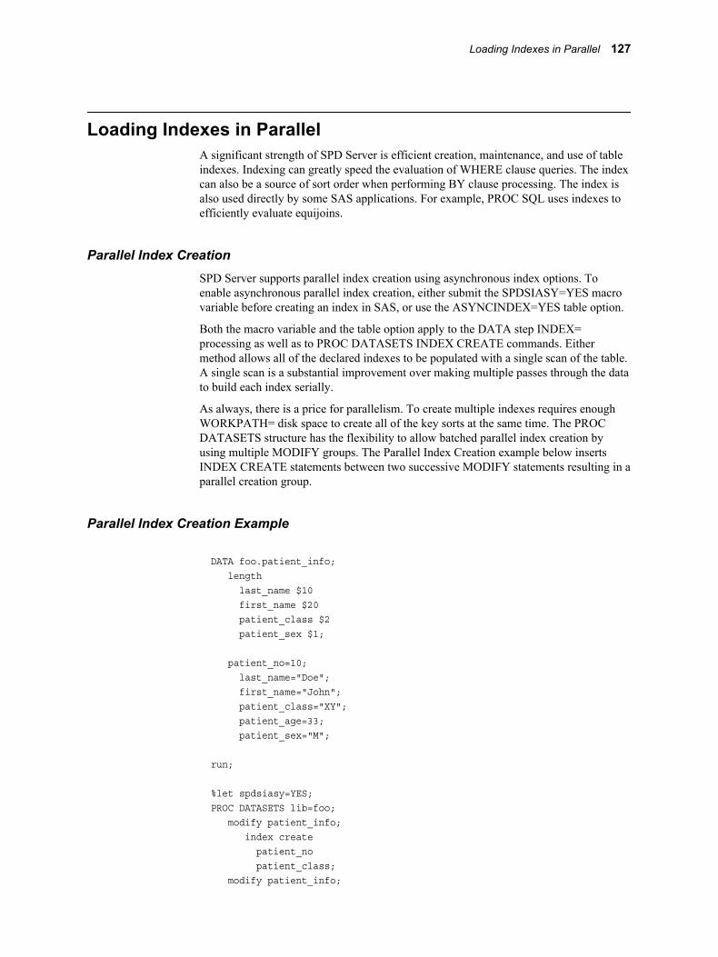
Loading Indexes in ParallelA significant strength of SPD Server is efficient creation, maintenance, and use of table indexes. Indexing can greatly speed the evaluation of WHERE clause queries. The index can also be a source of sort order when performing BY clause processing. The index is also used directly by some SAS applications. For example, PROC SQL uses indexes to efficiently evaluate equijoins.
Parallel Index CreationSPD Server supports parallel index creation using asynchronous index options. To enable asynchronous parallel index creation, either submit the SPDSIASY=YES macro variable before creating an index in SAS, or use the ASYNCINDEX=YES table option.
Both the macro variable and the table option apply to the DATA step INDEX= processing as well as to PROC DATASETS INDEX CREATE commands. Either method allows all of the declared indexes to be populated with a single scan of the table. A single scan is a substantial improvement over making multiple passes through the data to build each index serially.
As always, there is a price for parallelism. To create multiple indexes requires enough WORKPATH= disk space to create all of the key sorts at the same time. The PROC DATASETS structure has the flexibility to allow batched parallel index creation by using multiple MODIFY groups. The Parallel Index Creation example below inserts INDEX CREATE statements between two successive MODIFY statements resulting in a parallel creation group.
Parallel Index Creation Example
DATA foo.patient_info; length last_name $10 first_name $20 patient_class $2 patient_sex $1;
patient_no=10; last_name="Doe"; first_name="John"; patient_class="XY"; patient_age=33; patient_sex="M";
run;
%let spdsiasy=YES; PROC DATASETS lib=foo; modify patient_info; index create patient_no patient_class; modify patient_info;
Loading Indexes in Parallel 127

index create last_name first_name; modify patient_info; index create whole_name=(last_name first_name) class_sex=(patient_class patient_sex); quit;
Indexes for PATIENT_NO and PATIENT_CLASS are created in parallel, indexes for LAST_NAME and FIRST_NAME are created in parallel, and indexes for WHOLE_NAME and CLASS_SEX are created in parallel.
Parallel Index UpdatesSPD Server also supports parallel index updates during Table Append operations. Multiple threads enable overlap of data transfer to the proxy, as well as updates of the data store and index files. SPD Server decomposes Table Append operations into a set of steps that can be performed in parallel. The level of parallelism attained depends on the number of indexes that are present on the table. The more indexes you have, the greater the exploitation of parallelism during the append processing. As with parallel index creation, parallel index updates use WORKPATH= disk space for the key sorts that are part of the index append processing.
Truncating TablesThe Truncate command is a PROC SPDO command that allows the deletion of all rows in a table without deleting the table structure or metadata.
%let host=kaboom ;%let port=5191 ;%let domain=path2 ;
LIBNAME &domain sasspds "&domain" server=&host..&port user='anonymous' ip=YES ;/* create a table */data &domain..staceys_table ;
do i = 1 to 100 ; output ;end ;run ;
* verify the contents of the created table */
PROC CONTENTS data=&domain..staceys_table ;run ;
/* SPDO Truncate command deletes the table *//* data but leaves the table structure in *//* place so new data can be appended */PROC SPDO lib=&domain ;
128 Chapter 8 • Optimizing SAS Scalable Performance Data Server (SPD) Server

set acluser ;Truncate staceys_table ;
quit ;
* verify that no rows or data remain in *//* the structure of staceys_table */PROC CONTENTS data=&domain..staceys_table ;run ;
Optimizing WHERE Clauses
Overview of Optimizing WHERE ClausesSPD Server includes more advanced methods to optimize WHERE clauses. Before SPD Server 4.0, the rule-based, heuristic WHERE clause planner WHINIT was used to manually tune queries for performance. SPD Server provides dynamic WHERE clause costing, an automatic feature that can replace the need to manually tune queries. SPD Server dynamic WHERE-costing uses factors of cardinality and distribution to calculate relative processor costs of various WHERE clause options. SPD Server administrators can set server parameter commands in the spdsserv.parm file, or users can set macro variables to turn dynamic WHERE-costing on and off. If dynamic WHERE-costing is turned off, SPD Server reverts to using the rules-based WHERE clause planner.
WHERE Clause Definitions and Terminology• WHERE clauses are selection criteria for a query that specify one or more Boolean
predicates. Implementing the criteria, SPD Server selects only records that satisfy the WHERE clause.
• Predicates are the building blocks of WHERE clauses. Use them stand-alone or combine them with the operators AND and OR to form complex WHERE clauses. Here is an example of a WHERE clause:
"where x > 1 and y in (1 2 3)"
In this example, there are two predicates, x > 1 and y in (1 2 3). You specify the negative of a predicate by using not. For example, where x > 1 and not (y in (1 2 3)).
• Boolean logic determines whether two predicates, joined with an AND or OR, are true (satisfies the specification), or false (does not satisfy the specification). The AND operator requires that all predicates be true for the entire expression to be true. For example, the expression p1 AND p2 AND p3, is true only if all three predicates (p1, p2, andp3) are true. In contrast, the OR operator requires only one predicate to be true for the entire expression to be true.
For the WHERE clause (x < 5 or y in (1 2 3)) and z = 10, the following truth table describes the overall result (truth):
"x < 5 ?" "y in (1 2 3) ?" "z = 10 ?" Result========= ================ ========== ====== False False False False False False True False
Optimizing WHERE Clauses 129

False True False False False True True True True False False False True False True True True True False False True True True True
• Indexes are structures associated with tables that permit SPD Server to quickly access records that satisfy an indexed predicate. In an example WHERE clause, where x = 10 and y > 11, SPD Server selects the best index on column x to directly retrieve records that have a value of 10 in the x column. If no index exists for x, SPD Server must sequentially read each record in the table searching for x equal to 10.
• Simple and composite indexes: Simple indexes index a single column; composite indexes index two or more columns. The list of column(s) in an index is sometimes called the index key.
• Parallelism is the SPD Server capability that enables multiple threads to execute in parallel. Using multiple processors in parallel mode is sometimes called 'divide and conquer' processing. SPD Server uses parallelism to evaluate the multiple indexes that are involved in more complicated WHERE clauses.
SPD Server Indexing
Overview of Server IndexingSPD Server tables can have one or more indexes. There is a combination of four different indexing strategies a table can use, and the choice depends on the data populating the table, the size of the table, and the types of queries that will be executed against the table.
SPD Server indexing evaluates the processor cost of a WHERE clause. The section “WHERE-Costing Using Cardinality Ratio and Distribution Values” on page 133 shows how factors of cardinality and distribution are used to choose the evaluation strategy that will perform the WHERE clause at the smallest processor cost. The five evaluation strategies that the WHERE clause planner uses are EVAL 1, EVAL 2, EVAL 3, EVAL 4, and EVAL 5. The different EVAL strategies calculate the number of rows that will be required to execute a given query.
True rows are rows that contain the variable values specified in a WHERE clause. False rows do not contain the variable value specified in the clause. EVAL 1, EVAL 3, EVAL 4, and EVAL 5 evaluate true rows in the table using indices. EVAL 2 evaluates true rows of a table without using indices. EVAL strategies are explored in more detail in “WHERE Clause EVAL Strategies” on page 134.
SPD IndexesSPD Server uses segmented indices. A segmented index is created by dividing the index of a table into equally sized ranges of rows. Each range of rows is called a segment, or slot. You use the SEGSIZE= setting to define the size of the segment. A series of sub-indices each point to blocks of rows in the table. By default, SPD Server creates an index segment for every 8192 rows in a table.
The SPD segmented index facilitates SPD Server's parallel evaluation of WHERE clauses with an indexed predicate. First, the SPD index supports a pre-evaluation phase
130 Chapter 8 • Optimizing SAS Scalable Performance Data Server (SPD) Server

to determine which segments contain values that satisfy the predicate. Pre-evaluation speeds queries by eliminating segments that do not contain any possible values. Then, a number of threads up to the value of the SPDSTCNT= variable are launched to query the remaining index segments. The threads query the segments of the SPD index in parallel to retrieve the segment rows that satisfy the predicate. When all segments have been queried, the per-segment results are accumulated to determine the rows that satisfy the predicate. If the query contains multiple indexed predicates, then those predicates are also evaluated in parallel. When all predicates have been completed, their results are accumulated to determine the rows that satisfy the query.
MINMAX Variable ListSPD Server has a table option called MINMAXVARLIST=. The primary purpose of MINMAXVARLIST= is for use with SPD Server dynamic cluster tables, where specific members in the dynamic cluster contain a set or range of values, such as sales data for a given month. When an SPD Server SQL subsetting WHERE clause specifies specific months from a range of sales data, the WHERE planner checks the MIN and MAX variable list. Based on the MIN and MAX list information, the SPD Server WHERE planner includes or eliminates member tables in the dynamic cluster for evaluation.
Use the MINMAXVARLIST= table option with either numeric or character-based columns. MINMAXVARLIST= uses the list of columns that you submit to build a variable list. The MINMAXVARLIST= list contains only the minimum and maximum values for each column. The WHERE clause planner uses the index to filter SQL predicates quickly, and to include or eliminate member tables belonging to the cluster table from the evaluation.
Although the MINMAXVARLIST= table option is primarily intended for use with dynamic clusters, it also works on standard SPD Server tables. MINMAXVARLIST= can help reduce the need to create many indexes on a table, which can save valuable resources and space.
The MINMAXVARLIST= table option is available only when a table is being created or defined. If a table has a MINMAXVARLIST= variable list, moving or copying the table will destroy the variable list unless MINMAXVARLIST= is specified in the table output.
%let domain=path3 ;%let host=kaboom ;%let port=5201 ;
LIBNAME &domain sasspds "&domain" server=&host..&port user='anonymous' ;
/* Create three tables called *//* xy1, xy2, and xy3. */
data &domain..xy1(minmaxvarlist=(x y)); do x = 1 to 10; do y = 1 to 3; output; end;end;run;
data &domain..xy2(minmaxvarlist=(x y));
SPD Server Indexing 131
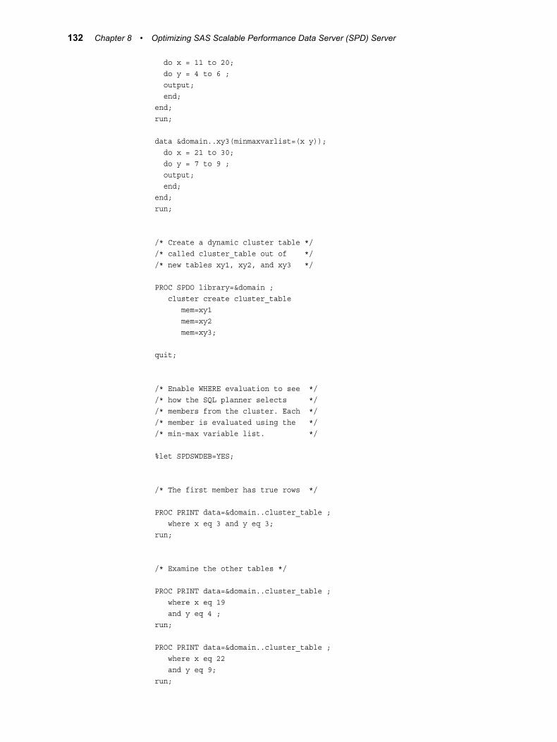
do x = 11 to 20; do y = 4 to 6 ; output; end;end;run;
data &domain..xy3(minmaxvarlist=(x y)); do x = 21 to 30; do y = 7 to 9 ; output; end;end;run;
/* Create a dynamic cluster table *//* called cluster_table out of *//* new tables xy1, xy2, and xy3 */
PROC SPDO library=&domain ; cluster create cluster_table mem=xy1 mem=xy2 mem=xy3; quit;
/* Enable WHERE evaluation to see *//* how the SQL planner selects *//* members from the cluster. Each *//* member is evaluated using the *//* min-max variable list. */
%let SPDSWDEB=YES;
/* The first member has true rows */
PROC PRINT data=&domain..cluster_table ; where x eq 3 and y eq 3;run;
/* Examine the other tables */
PROC PRINT data=&domain..cluster_table ; where x eq 19 and y eq 4 ;run;
PROC PRINT data=&domain..cluster_table ; where x eq 22 and y eq 9;run;
132 Chapter 8 • Optimizing SAS Scalable Performance Data Server (SPD) Server
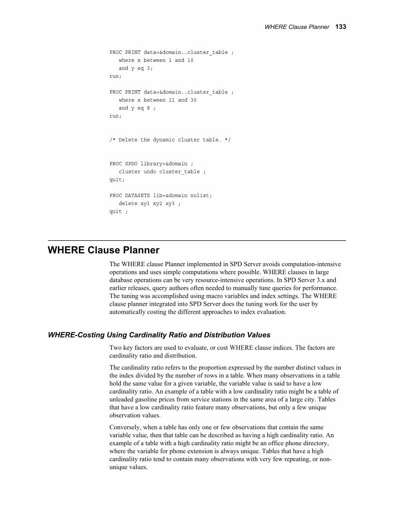
PROC PRINT data=&domain..cluster_table ; where x between 1 and 10 and y eq 3;run;
PROC PRINT data=&domain..cluster_table ; where x between 11 and 30 and y eq 8 ;run;
/* Delete the dynamic cluster table. */
PROC SPDO library=&domain ; cluster undo cluster_table ;quit;
PROC DATASETS lib=&domain nolist; delete xy1 xy2 xy3 ;quit ;
WHERE Clause PlannerThe WHERE clause Planner implemented in SPD Server avoids computation-intensive operations and uses simple computations where possible. WHERE clauses in large database operations can be very resource-intensive operations. In SPD Server 3.x and earlier releases, query authors often needed to manually tune queries for performance. The tuning was accomplished using macro variables and index settings. The WHERE clause planner integrated into SPD Server does the tuning work for the user by automatically costing the different approaches to index evaluation.
WHERE-Costing Using Cardinality Ratio and Distribution ValuesTwo key factors are used to evaluate, or cost WHERE clause indices. The factors are cardinality ratio and distribution.
The cardinality ratio refers to the proportion expressed by the number distinct values in the index divided by the number of rows in a table. When many observations in a table hold the same value for a given variable, the variable value is said to have a low cardinality ratio. An example of a table with a low cardinality ratio might be a table of unleaded gasoline prices from service stations in the same area of a large city. Tables that have a low cardinality ratio feature many observations, but only a few unique observation values.
Conversely, when a table has only one or few observations that contain the same variable value, then that table can be described as having a high cardinality ratio. An example of a table with a high cardinality ratio might be an office phone directory, where the variable for phone extension is always unique. Tables that have a high cardinality ratio tend to contain many observations with very few repeating, or non-unique values.
WHERE Clause Planner 133
The cardinality ratio for an index is in the range 0–1. Indices with a high cardinality ratio value of 1.0 are completely unique with no repeated values. Indices with a low cardinality ratio generate a score that approaches zero as the number of unique variable values diminish. The closer to zero, the lower the cardinality ratio of the index.
Distribution refers to the sequential proximity between observations for values of a variable that are repeated throughout the variable's data set distribution. When a certain value for a variable exists in many observations that are scattered uniformly throughout the table, that value is said to have a wide distribution. If a variable value exists in many contiguous or nearly contiguous rows, the distribution is clustered.
WHERE Clause EVAL StrategiesSPD Server indexing keeps track of the cardinality ratio and distribution of variable values in a table and uses them to calculate the cost of a WHERE clause. The WHERE clause planner uses four evaluation strategies to determine the number of rows that will be required to execute a given query. The four evaluation strategies are EVAL 1, EVAL 2, EVAL 3, and EVAL 4. True rows are rows that contain the variable values specified in a WHERE clause. False rows do not contain the variable value specified in the clause.
EVAL 1, EVAL 3, EVAL 4, and EVAL 5 evaluate true rows in the table using indices. EVAL 2 evaluates true rows of a table without using indices.
• EVAL 1 evaluates true rows using an index to locate the true rows in each segment of the table. The index evaluation process generates a list of row IDs per segment. EVAL 1 accepts WHERE clause operators for equivalency expressions such as EQ, =, LE, <=, LT, <, GE, >=, GT, >, IN, and BETWEEN. EVAL 1 uses threaded parallel processing across the index segments to permit concurrent evaluation of multiple indices. EVAL 1 combines multiple segment bitmaps from queries that use multiple indices to generate the list of row IDs per segment.
• EVAL 2 takes true rows as determined by EVAL 1, EVAL 3, or EVAL 4, and then uses brute force to eliminate any rows shown to be false, leaving a table that contains only true rows. EVAL 2 processes all rows of a table when no index evaluation is possible. For example, no index evaluation is possible when an index is not present or when some predecessor function performs an operation that invalidates the index.
• EVAL 3 is a single index sequential process. Use EVAL 3 when the number of rows returned by an index is unique or nearly unique (when cardinality ratio is high). EVAL 3 returns a list of true rows for the entire table. EVAL 3 only supports the equality operators EQ and =.
• EVAL 4 is similar to EVAL 3 but supports a larger set of inequality and inclusion operators, such as IN, GT, GE, LT, LE, and BETWEEN.
• EVAL 5 can operate when the SPD Server Index Scan facility is used. The EVAL 5 strategy uses index metadata and aggregate SQL functions to evaluate true rows. The EVAL 5 strategy does not require a table scan.
For example, when x is indexed, and SPD Server uses EVAL 5 to evaluate the SQL expression
count(*) where x=5 ,
the index metadata is scanned for the condition, x = 5 instead of performing table scans. The EVAL 5 strategy supports the min(), max(), count(), count(distint), nmiss(), and range() functions. The EVAL 5 strategy cannot be used on SQL expressions, which use functions other than those listed above.
The WHERE clause planner in SPD Server 3.x relied heavily on EVAL 1 and EVAL 2 threaded strategies to evaluate most clauses. Sometimes the SPD Server 3.x EVAL 1 and
134 Chapter 8 • Optimizing SAS Scalable Performance Data Server (SPD) Server
EVAL 2 strategies would over-thread and over-manipulate indices during the evaluations during WHERE clause evaluation. This resulted in reduced performance or excessive resource consumption. With SPD Server 5.1's WHERE clause costing in place, EVAL 3 and EVAL 4 strategies are more suitable evaluation engines which conserve resources and boost processor performance.
Assigning EVAL Strategies
Overview of Assigning EVAL StrategiesThe SPD Server WHERE clause planner uses the following logic when selecting an EVAL strategy to evaluate expressions:
When the planner encounters a WHERE clause, it builds a tree that represents all of the possible predicate expressions. The objective of the WHERE clause planner is to divide the set of predicate expressions into two trees. One tree collects predicate expressions that lack usable indices and are constrained to EVAL 2 evaluation. The remaining predicate expressions are put in the other tree. Each of the predicate expressions in the second tree is scanned and assigned an evaluation strategy of EVAL 1, EVAL 3, or EVAL 4, depending on the WHERE clause costing values and the syntax used in the predicate expression .
The second tree, which does not use the EVAL 2 method, is scanned for predicate expressions that return values with a low cardinality ratio. When low cardinality ratio predicate expressions are identified, they are ranked. The predicate expression with the lowest cardinality ratio value is set aside for an index-based evaluation. All of the other remaining predicate expressions are evaluated using the EVAL 2 tree strategy. The predicate expression with the highest cardinality ratio is evaluated using either the EVAL 3 or the EVAL 4 strategy. The syntax used in the predicate expression determines which of the two strategies to use. Frequently, the single index EVAL 3 or EVAL 4 is chosen because single index evaluations require smaller processing loads and yield reliable results. With a low processor overhead and a high data yield, there is no reason to include other indices when a single index is sufficient.
When the WHERE clause planner determines that no predicate expressions meet the low cardinality ratio criteria, it chooses the EVAL 1 strategy. Before the EVAL 1 operation is performed, the costing algorithm is run on the remaining predicates to prune any predicate expressions that represent large processor loads and large data yields. Predicate expressions that will require large processor loads and produce large data yields are moved to the EVAL 2 tree.
Index Scan FacilityWhen SPD Server invokes the Index Scan facility, and the SQL aggregate uses the specified supported functions for EVAL 5, the EVAL 5 strategy uses a fast index metadata scan to select SQL statements that meet the aggregate function criterion.
High Yield Predicate ExpressionsA large, or high data yield expression has a high percentage of rows containing true segments. The default threshold for a high yield expression is one where less than 25% of the rows evaluated are returned by the predicate. At this point, processor costs related to index use begin increasing without proportional returns on the evaluation results.
High Processing Load Predicate ExpressionsPredicate expressions that require high processing loads are predicates that usually require large amounts of index manipulation before they can complete. When the
WHERE Clause Planner 135
amount of index work that is required exceeds the work that is required to use an EVAL 2 strategy, the predicate expression will be best evaluated by the EVAL 2 tree. Open-ended predicate expressions that contain many syntax inequality operators such as GT and LT or many variations in syntax are good high work candidates for EVAL 2. High work predicate expressions are detected by comparing the number of unique values in the predicate expression to the number of unique values contained in the index.
High Yield and High Processing Load Predicate ExpressionsWhen all predicate expressions in EVAL 1 are high yield or high processor load, SPD Server uses segmented costing. In segmented costing, true segments are passed to EVAL 2 for processing. EVAL 2 only processes table segments that can provide true rows for the WHERE clause.
Turning WHERE Clause Costing OffYou can use the SPD Server spdsserv.parm parameter file to configure the default WHERECOSTING parameter setting to ON. If you want to turn off WHERE clause costing within the scope of a job, you can use macros or a DATA step to turn WHERE clause costing off and on:
• The SPDSWCST=NO macro setting turns off WHERE clause costing.
• The SPDSWSEQ=YES macro overrides WHERE clause costing and enables you to force a global EVAL3 or EVAL4 strategy.
• The WHERECOSTING parameter can be removed or set to NOWHERECOSTING in the spdsserv.parm file if you want to turn off costing for the entire server.
If you turn off WHERE clause costing in the spdsserv.parm parameter file, or if you use the macro setting SPDSWCST=NO, the WHERE clause planner reverts to the rules-based WHERE clause planning of earlier versions of SPD Server.
WHINIT: Indexed and Non-Indexed Predicates
Overview of WHINITIf SPD Server is not configured to use dynamic WHERE-costing, the WHERE clause planner reverts to the rule-based heuristics of WHINIT. WHINIT uses rules to select indexes for the predicates, and then select the most appropriate EVAL strategy for the query.
WHINIT splits the WHERE clause, represented as a tree, into non-indexed and indexed parts. Non-indexed predicates include
• non-indexed columns
• functions
• columns that have indexes that WHINIT cannot use
If the WHERE clause planner places indexed predicates in the non-indexed tree, it is usually because the predicates involve an OR expression. An example of a predicate with an OR expression is, where x = 1 or y = 2. Even if column x is indexed, WHINIT cannot use the index because the OR is disjunctive. As a result of the disjunctive OR, the planner cannot use the index, and places both the predicates x = 1 and y = 2 into the non-indexed part of the WHERE tree.
136 Chapter 8 • Optimizing SAS Scalable Performance Data Server (SPD) Server

Sample WHINIT OutputSAS users can use an SPD Server macro variable to view WHERE clause planner output:
%let SPDSWDEB=YES;
The following is what the WHINIT plan might give for the following scenario:
• a WHERE clause of where a = 1 and b in (1 2 3) and d = 3 and (d + 3 = c)
• an SPD index IDX_ABC on columns (A B C)
• an SPD index D on column (D)
Note: The line numbers are for reference; they are NOT part of the actual output.
1:whinit: WHERE ((A=1) and B in (1, 2, 3) and (D=3) and (C=(D+3))) 2:whinit: wh-tree presented 3: /-NAME = [A] 4: /-CEQ----| 5: | \-LITN = [1] 6: --LAND---| 7: | /-NAME = [B] 8: |--IN-----| 9: | | /-LITN = [1]10: | \-SET----|11: | |--LITN = [2]12: | \-LITN = [3]13: | /-NAME = [D]14: |--CEQ----|15: | \-LITN = [3]16: | /-NAME = [C]17: \-CEQ----|18: | /-NAME = [D]19: \-AADD---|20: \-LITN = [3]21:whinit: wh-tree after split22: /-NAME = [C]23: --CEQ----|24: | /-NAME = [D]25: \-AADD---|26: \-LITN = [3]
WHERE Clause Planner 137

27:whinit: SBM-INDEX D uses 50% of segs (WITHIN maxsegratio 75%)28:whinit: INDEX tree after split29: /-NAME = [A] <1>SBM-INDEX IDX_ABC (A,B)30: /-CEQ----|31: | \-LITN = [1]32: --LAND---|33: | /-NAME = [B]34: |--IN-----|35: | | /-LITN = [1]36: | \-SET----|37: | |--LITN = [2]38: | \-LITN = [3]39: | /-NAME = [D] <2>SBM-INDEX D (D)40: \-CEQ----|41: \-LITN = [3]42:whinit returns: ALL EVAL1(w/SEGLIST) EVAL2
Line 1 shows what the WHINIT Planner received. Do not be surprised -- what the Planner receives can differ from your entries. Sometimes SAS optimizes or transforms a WHERE clause before passing it to SPD Server. For example, it can eliminate entities such as NOT operators, the union of set lists, and so on.
Lines 2 to 20 show the presented WHERE clause in a tree format. The tree format is a user-readable form of the actual WHERE clause that is processed by the SPD Server engine.
Lines 21 to 26 show the non-indexed WHERE tree, the result of splitting off the indexed part. The non-indexed WHERE tree can be empty or it can look the same as lines 2 to 20 if no indexes are selected. Consider that it is the non-indexed part of the WHERE clause that WHINIT uses to filter records obtained by the indexed strategies (EVAL1, 3 or 4).
Lines 27 to 41 shows that the percentage of segments containing values selected from column D is with the maximum allowed to proceed with pre-segment logic. Therefore, only those segments that contain values that satisfy the WHERE clause for column D will be included in further query processing for that column. Composite index IDX_ABC and simple index D are used to resolve the indexed WHERE clause predicates.
Line 42, the last line in our output, shows which strategies are used. The first keyword ALL indicates that SPD Server can identify correctly ALL resulting records, without help from the SAS System. First, SPD Server will call EVAL1, an indexed method, to quickly access a list of records that satisfy where a = 1 and b in (1 2 3) and d = 3, then it will use EVAL2 to determine whether c = d + 3 is true on these records.
When output from EVAL1 displays the suffix w/ seglist, as it does in the above output, it means that SPD indexes were detected, and that the indexes were used to filter only the segments that satisfy the indexed predicates. When EVAL1 has no suffix, it means that ALL segments will be evaluated.
138 Chapter 8 • Optimizing SAS Scalable Performance Data Server (SPD) Server

SPD Server stores the minimum and maximum values for a table index in a global structure. WHINIT can use the numeric range to 'prune' predicates when the table index values are out of the min / max range. WHINIT output keywords can indicate pruning activity. For example, if WHINIT had determined that the values for D (in our WHERE clause) are between 5 and 13, then as a consequence, the predicate where d = 3 could never be true. In this case, WHINIT would have pruned this predicate because it is logically impossible, or FALSE. Pruning can also affect higher nodes. If the d = 3 predicate were deemed FALSE, then the AND sub tree would also be FALSE and would also have been pruned.
WHINIT Output Return KeywordsIn the last line of the output, ALL is one of the following keywords that the Planner can display:
• ALL - SPD Server can evaluate ALL of the WHERE clause when determining which records satisfy the clause.
• SOME - SPD Server can handle SOME or part of the WHERE clause; it will then need SAS to help identify resulting records.
• NONE - SPD Server cannot evaluate this WHERE clause; SAS will perform all evaluations.
• TRUE - SPD Server has determined that the entire WHERE clause is TRUE, and that all the records satisfy the given WHERE clause.
• FALSE - SPD Server determined that the WHERE clause is FALSE, that is, no records can satisfy the WHERE clause.
• RC=number - An internal error has occurred; the error number is displayed.
• EVALx - the EVAL strategies the planner will use; x can be 1, 2, 3, or 4.
Composite Index PermutationsA composite index can involve one or more in set equality predicates, such as an index on columns (a b c). When WHINIT is presented with a WHERE clause that has such a composite index, such as where a = 1 and b in (1 2 3) and c in (4 5), it will generate all permutations of this compound key, probing the index for each value. In our example, six values are generated:
(a b c) = (1 1 4) (1 1 5) (1 2 4) (1 2 5) (1 3 4) (1 3 5)
The permutations start at the back end of the key to take advantage of locality: to locate keys with close values that access the same disk page. This means less input/output operations on the index.
How to Affect the WHERE Planner
Macro Variable SPDSWCST=To turn off dynamic WHERE-costing, specify
%let SPDSWCST=NO;
How to Affect the WHERE Planner 139
Macro Variable SPDSWDEB=To turn on WHINIT planning output, specify
%let SPDSWDEB=YES;
Macro Variable SPDSIRAT=To affect the WHERE planner SPD index pre-evaluation, specify To affect the WHERE planner SPD index pre-evaluation, specify To affect the WHERE planner SPD index pre-evaluation, specify
%let SPDSIRAT=index-segment-ratio;
The SPDSIRAT= macro variable specifies a maximum percentage (ratio) for the number of segments in the hybrid bitmap that must contain the index value before the WHERE planner should pre-evaluate a segment list.
The segment list enables the planner to launch threads only for segments that contain the value. If the value number exceeds the ratio, the planner performs no pre-evaluation. Instead, the planner launches a thread for each segment in the table.
The SPDSIRAT= macro variable option can be used to ensure that time spent in pre-evaluation does not exceed the cost of launching a thread for each segment in the table. By default SPDSIRAT= is set to 75%. This means that if an index value is contained in 75% or less of the index segments, the hybrid bitmap logic will pre-evaluate the value and return a list of segments to the WHERE clause planner. If more than 75% of the index segments contain the target index value, the time spent on pre-evaluation might be more than the time saved by skipping a small number of segments.
For some tables 75% might not be the optimal setting. To determine a better setting, run a performance benchmark, adjust the percentage, and rerun the performance benchmark. Comparing results will show you how the specific data population that you are querying responds to shifting the index-segment ratio. The allowable range to adjust the setting value is from 0 to 100, where 0 means never perform WHERE clause pre-evaluation, and 100 means always perform WHERE clause pre-evaluation.
Macro Variable SPDSNIDX= or Table Option NOINDEX=To suppress WHINIT use of any index, specify the no index SPD Server macro variable or the corresponding SPD Server table option:
%let SPDSNIDX=YES;
data _null_;set foo.a (noindex=yes);
Macro Variable SPDSWSEQ=By default, when WHINIT detects equality predicates that have indexes, it chooses EVAL1. However, the user can decide that sequential EVAL3 or EVAL4 methods are better. For example, in an equality WHERE predicate such as where x = 3, WHINIT will default to EVAL1 to evaluate the clause. If a user knows that the table queried has only a
140 Chapter 8 • Optimizing SAS Scalable Performance Data Server (SPD) Server
few records that can satisfy this predicate, EVAL3 might be a better choice. To force WHINIT to choose EVAL3/4, specify:
%let SPDSWSEQ=YES;
Server Parameter Option [NO]WHERECOSTINGControls whether the server uses dynamic WHERE-costing. When dynamic WHERE-costing is disable, the rules-based WHINIT heuristic is used to tune WHERE clauses for performance. The default setting is for NOWHERECOSTING.
WHERENOINDEX OptionA user might decide that one or more indexes selected by a WHINIT plan are not the best choice. This can occur because WHINIT is rule-based, not cost-based. Sometimes WHINIT selects a less-than-optimal plan. WHINIT's use of specific indexes can be affected by specifying the SPD Server option WHERENOINDEX= in your DATA step.
data _null_;set foo.a (wherenoindex=(idx_abc d))
This example specifies that WHINIT not use index idx_abc and index d.
When and Why Should I Suppress Indexes?Most rule-based planners, including WHINIT from SPD Server, assume that the index has a uniform distribution of values between the upper and lower value boundaries. This means if data values range between 2 and 10, that there are an equal number of 3s and 4s, and so on. When the assumption of a uniform distribution is false, an indexed predicate can return a large number of records. In turn, this causes WHINIT's indexed plan to run slower than a sequential read of the entire table. In this case the index should be suppressed.
Here is another, more subtle instance. When the WHERE clause uses only the front part of the key, WHINIT selects a composite index. Assume an index abcd on columns A, B, C, and D, and an index e on column E, and specify the WHERE clause
where a = 3 and e = 5;
Normally, WHINIT will select both indexes (abcd and e) and choose EVAL1. However, using the index abcd just to interrogate 'a' might return a large number of records. In this case, suppressing the abcd index might be a good idea. If so, WHINIT will still choose EVAL1 for e = 5, or EVAL3 if SPDSWEV1=NO, and EVAL2, the post-filter, for a = 3.
Identical Parallel WHERE Clause Subsetting Results
Overview of Parallel WHERE Clause SubsettingUnder certain circumstances, it is possible to perform parallel WHERE clause subsetting on a table more than once and to receive slightly different results. This event can occur
Identical Parallel WHERE Clause Subsetting Results 141

when submitting parallel WHERE clause code to SPD Server that uses the SAS OBS=nnnn data set option.
The SAS OBS=nnnn data set option causes processing to end with the specified (nth) observation in a table. Because parallel WHERE clause processing is threaded, subsetting a table and using OBS=nnnn might not produce identical results from run to run, or different batch jobs using the same WHERE clause code might produce slightly different results.
When a parallel WHERE-cause evaluation is split into multiple threads, SPD Server uses a multi-threading model that is designed to return rows as fast as possible. Some threads might be able to complete row scans incrementally faster than other threads, due to uneven loads across multiple processors or system contention issues. This inequity can create minute variances that can generate nonidentical results to the same subsetting request.
If you have code that performs parallel WHERE clause subsetting in conjunction with the OBS=nnnn data processing option, and if it is critical that successive WHERE clause subsets on the same data must be identical, you can eliminate thread contention error by setting the thread count value for that operation to 1.
To set the SPD Server thread count value, you can use the SPDSTCNT= macro:
%let SPDSTCNT=1;
The same potential for subsetting variation applies when a DATA step uses the OBS=nnnn data processing option with a parallel by-clause, such as:
data test1; set spds45.testdata (obs=1000); where j in (1,5,25); by i; run;
Use the SPDSTCNT= macro solution to ensure identical results across multiple identical table subsetting requests.
WHERE Clause Subsetting Variation ExampleJob 1 and Job 2 use the same tables and data requests but produce non-identical results as seen in the respective Job 1 and Job 2 outputs.
To eliminate variation in the output, simply add the thread count statement
%let SPDSTCNT=1;
to the beginning of each job.
Job 1 data test1; set spds45.testdata (obs=1000); where j in (1,5,25); run;
PROC SORT data=test1; by i; run;
142 Chapter 8 • Optimizing SAS Scalable Performance Data Server (SPD) Server
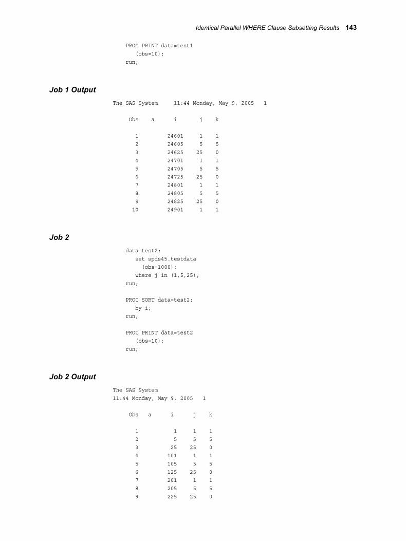
PROC PRINT data=test1 (obs=10); run;
Job 1 OutputThe SAS System 11:44 Monday, May 9, 2005 1
Obs a i j k
1 24601 1 1 2 24605 5 5 3 24625 25 0 4 24701 1 1 5 24705 5 5 6 24725 25 0 7 24801 1 1 8 24805 5 5 9 24825 25 0 10 24901 1 1
Job 2 data test2; set spds45.testdata (obs=1000); where j in (1,5,25); run;
PROC SORT data=test2; by i; run;
PROC PRINT data=test2 (obs=10); run;
Job 2 OutputThe SAS System11:44 Monday, May 9, 2005 1
Obs a i j k
1 1 1 1 2 5 5 5 3 25 25 0 4 101 1 1 5 105 5 5 6 125 25 0 7 201 1 1 8 205 5 5 9 225 25 0
Identical Parallel WHERE Clause Subsetting Results 143
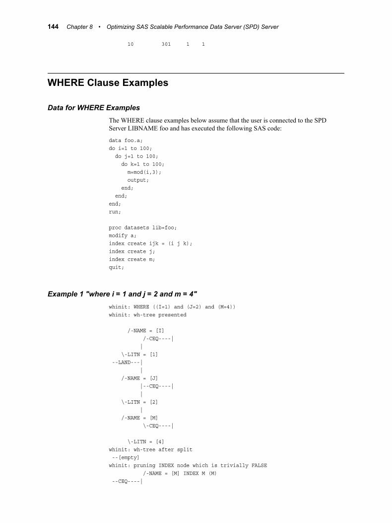
10 301 1 1
WHERE Clause Examples
Data for WHERE ExamplesThe WHERE clause examples below assume that the user is connected to the SPD Server LIBNAME foo and has executed the following SAS code:
data foo.a;do i=1 to 100; do j=1 to 100; do k=1 to 100; m=mod(i,3); output; end; end;end;run;
proc datasets lib=foo;modify a;index create ijk = (i j k);index create j;index create m;quit;
Example 1 "where i = 1 and j = 2 and m = 4"whinit: WHERE ((I=1) and (J=2) and (M=4))whinit: wh-tree presented
/-NAME = [I] /-CEQ----| | \-LITN = [1] --LAND---| | /-NAME = [J] |--CEQ----| | \-LITN = [2] | /-NAME = [M] \-CEQ----|
\-LITN = [4]whinit: wh-tree after split --[empty]whinit: pruning INDEX node which is trivially FALSE /-NAME = [M] INDEX M (M) --CEQ----|
144 Chapter 8 • Optimizing SAS Scalable Performance Data Server (SPD) Server

\-LITN = [4]whinit: INDEX tree evaluated to FALSEwhinit returns: FALSE
Here the only values that column M can contain are 0, 1, or 2. Thus, the predicate m = 4 is identified as trivially FALSE. Because this predicate is part of an AND predicate, it too is FALSE. Consequently, the entire WHERE clause is pre-evaluated to FALSE, meaning that no records can satisfy this WHERE clause. Thus, as a result of the pre-evaluation, no records are actually read from disk. This is an example of optimization at its best.
WHERE_EXAMPLE 2: where i in (1, 2, 3) and j in (4, 5, 6, 7) and k > 8 and m = 2
whinit: WHERE (I in (1, 2, 3) and J in (4, 5, 6, 7) and (K>8) and (M=2))whinit: wh-tree presented
/-NAME = [I] /-IN-----| | | /-LITN = [1] | \-SET----| | |--LITN = [2] | \-LITN = [3] --LAND---| | /-NAME = [J] |--IN-----| | | /-LITN = [4] | \-SET----| | |--LITN = [5] | |--LITN = [6] | \-LITN = [7] | /-NAME = [K] |--CGT----| | \-LITN = [8] | /-NAME = [M] \-CEQ----|
\-LITN = [2]whinit: SBM-INDEX M uses 60% of segs(WITHIN maxsegratio 100%)whinit: wh-tree after split /-NAME = [K] --CGT----| \-LITN = [8]
WHERE Clause Examples 145

whinit: INDEX tree after split
/-NAME = [I] <1>SBM-INDEX IJK (I,J) /-IN-----| | | /-LITN = [1] | \-SET----| | |--LITN = [2] | \-LITN = [3] --LAND---| | /-NAME = [J] |--IN-----| | | /-LITN = [4] | \-SET----| | |--LITN = [5] | |--LITN = [6] | \-LITN = [7] | /-NAME = [M] <2>SBM-INDEX M (M) \-CEQ----|
\-LITN = [2]whinit returns: ALL EVAL1(w/SEGLIST) EVAL2
Here, a composite index ijk was defined on columns (i j k). This composite index is used for column's i and j, which is an equality index predicate. Column k is not included because it involves an inequality operator (greater than). Because there are no other indexes for column k, this predicate is assigned to EVAL2 . EVAL2 will post-filter the records obtained through the use of indexes.
WHERE_EXAMPLE 3: where i = 1 and j > 5 and mod(k, 3) = 2 whinit: WHERE ((I=1) and (J>5) and (MOD(K, 3)=2))whinit: wh-tree presented
/-NAME = [I] /-CEQ----| | \-LITN = [1] --LAND---| | /-NAME = [J] |--CGT----| | \-LITN = [5] | /-FUNC = [MOD()]
146 Chapter 8 • Optimizing SAS Scalable Performance Data Server (SPD) Server

| /-FLST---| | | |--NAME = [K] | | \-LITN = [3] \-CEQ----|
\-LITN = [2]whinit: wh-tree after split
/-FUNC = [MOD()] /-FLST---| | |--NAME = [K] | \-LITN = [3] --CEQ----| \-LITN = [2]whinit: SBM-INDEX IJK uses 1% of sges(WITHIN maxsegratio 75%)whinit: SBM-INDEX J uses at least 76% of segs(EXCEEDS maxsegratio 75%)whinit: INDEX tree after split
/-NAME = [I] <1>SBM-INDEX IJK (I) /-CEQ----| | \-LITN = [1] --LAND---| | /-NAME = [J] <2>SBM-INDEX J (J) \-CGT----|
\-LITN = [5]whinit returns: ALL EVAL1(w/SEGLIST) EVAL2
Here the indexes on column i, a composite index on the columns (i j k), and the column j are combined. In this example WHINIT uses both EVAL1 and EVAL2. The j predicate involves an inequality operator (greater than). Therefore, WHINIT cannot combine the predicate with i and the composite index involving i and j (and k).
Using the composite index ijk in this plan might be inefficient. If a smaller composite index (that is, one on i j or a simple index on i) were available, WHINIT would select it. In lieu of this, try benchmarking the plan. Suppress the composite index and compare the results to the existing plan to see which is more efficient (faster) on your machine.
The example that follows shows what WHINIT's plan would look like with the composite index suppressed.
WHERE_Example 4: where i = 1 and j > 5 and mod(k, 3) = 2In this example, the index IJK is suppressed.
whinit: WHERE ((I=1) and (J>5) and (MOD(K, 3)=2))whinit: wh-tree presented
/-NAME = [I] /-CEQ----|
WHERE Clause Examples 147

| \-LITN = [1] --LAND---| | /-NAME = [J] |--CGT----| | \-LITN = [5] | /-FUNC = [MOD()] | /-FLST---| | | |--NAME = [K] | | \-LITN = [3] \-CEQ----|
\-LITN = [2]whinit: wh-tree after split
/-NAME = [I] /-CEQ----| | \-LITN = [1] --LAND---| | /-FUNC = [MOD()] | /-FLST---| | | |--NAME = [K] | | \-LITN = [3] \-CEQ----|
\-LITN = [2]whinit: SBM_INDEX J uses at least 76% of segs (EXCEEDS maxsegratio 75%)whinit: checking all hybrid segmentswhinit: INDEX tree after split /-NAME = [J] <1>SBM-INDEX J (J) --CGT----| \-LITN = [5]whinit returns: ALL EVAL1 EVAL2
Notice that the predicate involving column i is non-indexed. WHINIT evaluates it using EVAL2. Because the predicate j > 5 still uses an inequality comparison, WHINIT continues to use EVAL1. Finally, because the percentage of segments that contain values for column J exceeds the maximum segment ratio, pre-segment logic is not done on column J. As a result, all segments of the table are queried for values that satisfy the WHERE clause for column J.
148 Chapter 8 • Optimizing SAS Scalable Performance Data Server (SPD) Server

Server-Side Sorting
Overview of Server-Side SortingIn most instances, using a BY clause in SAS code submitted to an SPD Server table triggers a BY clause evaluation by SPD Server. This BY clause assertion to the SPD Server might or might not require sorting to produce the ordered rowset that the BY clause requires. In some cases, a table index can be used to sort the rows to satisfy a BY clause.
For example, the input table to a PROC SORT step is sorted in server context (by the associated LIBNAME proxy). The rows are returned to PROC SORT in BY clause order. In this case, PROC SORT knows that the data is already ordered, and writes the data to the output table without sorting it again. Unfortunately, this approach still must send the data from the LIBNAME proxy to the SAS client and then back to the LIBNAME proxy. However, there are other ways to use an SPD Server SQL pass-through COPY statement to avoid the overhead of the data round-trip.
SPD Server attempts to use an index when performing a BY clause. The software looks specifically for an index that has variables in the order specified in the BY clause. On the surface this seems like a good idea: table row order is already determined because the keys in the index are ordered. SPD Server reads the keys in order from the index, and then returns the rows from the table, based on the row IDs that are stored with the index key values.
Use caution when using BY clauses on tables that have indexes on their BY columns. Using the index is not always a good idea. When no suitable index exists to determine BY clause order, SPD Server uses a parallel table scan sort that keeps the table row intact with the sort key. The time required to access a highly random distribution of row IDs (obtained by using the index) can greatly exceed the time required to sort the rows from scratch.
When you use a WHERE clause to filter the rows from an SPD Server table with a BY clause to order them in a desired way, SPD Server handles both the subsetting and the ordering for this request. In this case, the filtered rows that were qualified by the WHERE clause are fed directly into a sort step. Feeding the filtered rows into the sort step is part of the parallel WHERE clause evaluation. The final ordered rowset is the result. In this case, the previous discussion of index use does not apply. Index use for WHERE clause filtering is very desirable and greatly improves the filtering performance that feeds into the sort step. Arbitrarily suppressing index use with a WHERE and BY combination should be avoided.
Suppressing the Use of IndexesSuppress the use of indexes on the BY clause by using the SPDSNIDX=YES macro variable or by asserting the NOINDEX=YES table option. Suppressing the use of the index can significantly improve time required to process a BY clause in SPD Server.
Advantages of Implicit Server SortsAn exceptional feature is the software's ability to execute ad hoc order-BY queries without pre-sorting the table on the BY variables. Many SAS job streams are structured
Server-Side Sorting 149

with code that alternates PROC SORT followed by PROC xxxx invocations, where the PROC SORT step is needed only for the execution of the PROC xxxx step.
When sort order is relevant only to the following step, eliminate the PROC SORT step and just use the BY clause on the PROC xxxx step. This eliminates the extra data transfer (to PROC SORT from SPD Server and then back from PROC SORT to SPD Server) to store the sorted result. Even if SPD Server performs the sort associated with the PROC SORT, there is extra data transfer. The data's round trip from the server to the SAS client and back can impose a substantial time penalty.
150 Chapter 8 • Optimizing SAS Scalable Performance Data Server (SPD) Server

Chapter 9
SAS Scalable Performance Data (SPD) Server Macro Variables
Introduction . . . . . . . . . . . . . . . . . . . . . . . . . . . . . . . . . . . . . . . . . . . . . . . . . . . . . . . . . 152
Variable for Compatibility with the Base SAS Engine . . . . . . . . . . . . . . . . . . . . . . 152SPDSBNEQ= . . . . . . . . . . . . . . . . . . . . . . . . . . . . . . . . . . . . . . . . . . . . . . . . . . . . . 152
Variables for Miscellaneous Functions . . . . . . . . . . . . . . . . . . . . . . . . . . . . . . . . . . . 153SPDSEOBS= . . . . . . . . . . . . . . . . . . . . . . . . . . . . . . . . . . . . . . . . . . . . . . . . . . . . . 153SPDSSOBS= . . . . . . . . . . . . . . . . . . . . . . . . . . . . . . . . . . . . . . . . . . . . . . . . . . . . . 154SPDSUSAV= . . . . . . . . . . . . . . . . . . . . . . . . . . . . . . . . . . . . . . . . . . . . . . . . . . . . . 154SPDSUSDS= . . . . . . . . . . . . . . . . . . . . . . . . . . . . . . . . . . . . . . . . . . . . . . . . . . . . . 155SPDSVERB= . . . . . . . . . . . . . . . . . . . . . . . . . . . . . . . . . . . . . . . . . . . . . . . . . . . . . 156SPDSFSAV= . . . . . . . . . . . . . . . . . . . . . . . . . . . . . . . . . . . . . . . . . . . . . . . . . . . . . 156SPDSEINT= . . . . . . . . . . . . . . . . . . . . . . . . . . . . . . . . . . . . . . . . . . . . . . . . . . . . . . 157
Variables for Sorts . . . . . . . . . . . . . . . . . . . . . . . . . . . . . . . . . . . . . . . . . . . . . . . . . . . 158SPDSBSRT= . . . . . . . . . . . . . . . . . . . . . . . . . . . . . . . . . . . . . . . . . . . . . . . . . . . . . 158SPDSNBIX= . . . . . . . . . . . . . . . . . . . . . . . . . . . . . . . . . . . . . . . . . . . . . . . . . . . . . . 159SPDSSTAG= . . . . . . . . . . . . . . . . . . . . . . . . . . . . . . . . . . . . . . . . . . . . . . . . . . . . . 160
Variables for WHERE Clause Evaluations . . . . . . . . . . . . . . . . . . . . . . . . . . . . . . . 160SPDSTCNT= . . . . . . . . . . . . . . . . . . . . . . . . . . . . . . . . . . . . . . . . . . . . . . . . . . . . . 160SPDSEV1T= . . . . . . . . . . . . . . . . . . . . . . . . . . . . . . . . . . . . . . . . . . . . . . . . . . . . . . 161SPDSEV2T= . . . . . . . . . . . . . . . . . . . . . . . . . . . . . . . . . . . . . . . . . . . . . . . . . . . . . . 162SPDSWDEB= . . . . . . . . . . . . . . . . . . . . . . . . . . . . . . . . . . . . . . . . . . . . . . . . . . . . . 163SPDSIRAT= . . . . . . . . . . . . . . . . . . . . . . . . . . . . . . . . . . . . . . . . . . . . . . . . . . . . . . 163SPDSNIDX= . . . . . . . . . . . . . . . . . . . . . . . . . . . . . . . . . . . . . . . . . . . . . . . . . . . . . 164SPDSWCST= . . . . . . . . . . . . . . . . . . . . . . . . . . . . . . . . . . . . . . . . . . . . . . . . . . . . . 165SPDSWSEQ= . . . . . . . . . . . . . . . . . . . . . . . . . . . . . . . . . . . . . . . . . . . . . . . . . . . . . 166
Variables That Affect Disk Space . . . . . . . . . . . . . . . . . . . . . . . . . . . . . . . . . . . . . . . 166SPDSCMPF= . . . . . . . . . . . . . . . . . . . . . . . . . . . . . . . . . . . . . . . . . . . . . . . . . . . . . 166SPDSDCMP= . . . . . . . . . . . . . . . . . . . . . . . . . . . . . . . . . . . . . . . . . . . . . . . . . . . . . 167SPDSIASY= . . . . . . . . . . . . . . . . . . . . . . . . . . . . . . . . . . . . . . . . . . . . . . . . . . . . . . 167SPDSSIZE= . . . . . . . . . . . . . . . . . . . . . . . . . . . . . . . . . . . . . . . . . . . . . . . . . . . . . . 168
Variables to Enhance Performance . . . . . . . . . . . . . . . . . . . . . . . . . . . . . . . . . . . . . 169SPDSNETP= . . . . . . . . . . . . . . . . . . . . . . . . . . . . . . . . . . . . . . . . . . . . . . . . . . . . . 169SPDSSADD= . . . . . . . . . . . . . . . . . . . . . . . . . . . . . . . . . . . . . . . . . . . . . . . . . . . . . 170SPDSSYRD= . . . . . . . . . . . . . . . . . . . . . . . . . . . . . . . . . . . . . . . . . . . . . . . . . . . . . 170SPDSAUNQ= . . . . . . . . . . . . . . . . . . . . . . . . . . . . . . . . . . . . . . . . . . . . . . . . . . . . . 171
Variable for a Client and a Server Running on the Same UNIX Machine . . . . . . 171SPDSCOMP= . . . . . . . . . . . . . . . . . . . . . . . . . . . . . . . . . . . . . . . . . . . . . . . . . . . . . 171
151

IntroductionIn Base SAS software, macro variables, known as symbolic variables, operate similarly to LIBNAME and table options. But, they have an advantage because they apply globally. That is, their value remains constant until explicitly changed. These variables can be used by the SPD Server LIBNAME to service the behavior of the client and server.
This chapter presents reference information for SPD Server macro variables, including their purpose, default values, and when and how to use them. The variables are grouped by function or purpose of the default value. Changing the value can also change the purpose, making the variable fall into another group.
For example, the default setting for the macro variable SPDSSADD= is NO. The SPDSSADD= macro enhances performance during data appends. Setting SPDSSADD= to YES changes the way the variable functions. The macro setting SPDSADD=YES ensures compatibility with the Base SAS engine. The default setting improves performance. Changing the setting from the default improves Base SAS software compatibility.
To set a macro variable to YES submit the following statement:
%let <macro-variable-name>=YES;
Note: Assignments for macro variables with YES|NO arguments must be entered in uppercase (capitalized).
When you specify table option settings, precedence matters. If you specify a table option after you set the option in a macro variable statement, the table option setting takes precedence over the macro variable option setting. If you specify an option using a LIBNAME statement, and then later specify an option setting through a macro variable statement, the table option setting made in the macro variable takes precedence over the LIBNAME statement setting.
To view the default values for the SPD Server macro variables, use the SPDSMAC command associated with PROC SPDO. SAS displays the macro variables and their current settings. Understanding proper use of macro variables in SPD Server allows you to unleash the power of the software.
Variable for Compatibility with the Base SAS Engine
SPDSBNEQ=Use the SPDSBNEQ= setting to specify the output order of table rows that have identical values in the BY column.
Syntax
SPDSBNEQ=YES|NO
Default: NO
Corresponding Table Option: BYNOEQUALS=
152 Chapter 9 • SAS Scalable Performance Data (SPD) Server Macro Variables
Arguments
YESoutputs rows with identical values in a BY clause in random order.
NOoutputs rows with identical values in a BY clause using the relative table position of the rows from the input table.
Description
SPDSBNEQ=NO configures the SPD Server to imitate the Base SAS engine behavior. If strict compatibility is not required, assign SPDSBNEQ=YES. Random output allows the SPD Server to create indexes and append to tables faster.
Example
Configure the SPD Server so that it output table rows as quickly as possible when processing rows that have identical values in the BY column.
%let SPDSBNEQ=YES;
Variables for Miscellaneous Functions
SPDSEOBS=Use the SPDSEOBS= macro variable to specify the number of the last row (end observation) of a user-defined range that you want to process in a table.
Syntax
SPDSEOBS=n
Default: The default setting of 0 processes the entire table.
Corresponding Table Option: ENDOBS=
Arguments
nis the number of the end row.
Description
The SPD Server processes the entire table by default unless you specify a range of rows. You can specify a range using the macro variables SPDSSOBS= and SPDSEOBS=, or you can use the table options, STARTOBS= and ENDOBS=.
If you use the range start macro variable SPDSSOBS= without specifying an end range value using the SPDSEOBS= macro variable, SPD Server processes to the last row in the table. If you specify values for both SPDSSOBS= and SPDSEOBS= macro variables, the value of SPDSEOBS= must be greater than SPDSSOBS=. The SPDSSOBS= and SPDSEOBS= macro variables specify ranges for table input processing as well as WHERE clause processing.
Example
In order to create test tables, you configure the SPD Server to subset the first 100 rows of each table in your job. Submit the macro variable statement for SPDSEOBS= at the beginning of your job.
%let SPDSEOBS=100;
Variables for Miscellaneous Functions 153

SPDSSOBS=Use the SPDSSOBS= macro variable to specify the number of the starting row (observation) in a user-defined range of a table.
Syntax
SPDSSOBS=n
Default: The default setting of 0 processes the entire table.
Corresponding Table Option: STARTOBS=
Arguments
nis the number of the start row.
Description
By default, SPD Server processes entire tables unless you specify a range of rows. You can specify a range using the macro variables SPDSSOBS= and SPDSEOBS=, or you can use the table options, STARTOBS= and ENDOBS=.
If you specify the end of a user-defined range using the SPDSEOBS= macro variable, but do not implicitly specify the beginning of the range using SPDSSOBS=, SPD Server sets SPDSSOBS= to 1, or the first row in the table. If you specify values for both SPDSSOBS= and SPDSEOBS= macro variables, the value of SPDSEOBS= must be greater than SPDSSOBS=. The SPDSSOBS= and SPDSEOBS= macro variables specify ranges for table input processing as well as WHERE clause processing.
Example
Print the INVENTORY.OLDAUTOS table, skipping rows 1-999, and beginning with row 1000. You should submit the SPDSSOBS= macro variable statement before the PROC PRINT statement in your job.
%let SPDSSOBS=1000;
The statement above specifies the starting row with SPDSSOBS=, but does not declare an ending row for the range using SPDSEOBS=. When the program executes, SAS will begin printing at row 1000 and continues until the final row of the table is reached.
PROC PRINT data=inventory.oldautos;run;
SPDSUSAV=Use the SPDSUSAV= macro variable to specify whether to save rows with nonunique (rejected) keys to a separate SAS table.
Syntax
SPDSUSAV=YES|NO|REP
Default: NO
Affected by Table Option : SYNCADD=
Use in Conjunction with Variable : SPDSUSDS=
Corresponding Table Option : UNIQUESAVE=
154 Chapter 9 • SAS Scalable Performance Data (SPD) Server Macro Variables

Arguments
YESwrites rows with nonunique key values to a SAS table. Use the macro variable SPDSUSDS= to reference the name of the SAS table for the rejected keys.
NOnonunique key values are ignored and rejected rows are not written to a separate table.
REPwhen updating a master table from a transaction table, where the two tables share identical variable structures, the SPDSUSAV=REP option replaces the updated row in the master table instead of appending a row to the master table. The REP option only functions in the presence of a /UNIQUE index on the MASTER table. Otherwise, the REP setting is ignored..
Description
When performing an append operation, SPD Server does not save the rows that contain duplicate key values unless the SPDSUSAV= macro variable is set to YES.
When SPDSUSAV= is set to YES, SPD Server creates a hidden SAS table and writes rejected rows to the table. Use the SPDSUSDS= macro variable command to view the contents of the table. Each Append operation creates a different table.
Example
Append several tables to the EMPLOYEE table, using employee number as a unique key. The appended tables should not have records with duplicate employee numbers.
At the beginning of the job, configure SPD Server to write any rejected (identical) employee number records to a SAS table. The macro variable SPDSUSDS= holds the name of the SAS table for the rejected keys.
%let SPDSUSAV=YES
Use a %PUT statement to display the name of the table, and then print the table.
%put Set the macro variable spdsusds to &spdsusds;
title 'Duplicate (nonunique) employee numbers found in EMPS';PROC PRINT data=&spdsusds run;
SPDSUSDS=Use the SPDSUSDS= macro variable to reference the name of the SAS table that SPD Server creates for duplicate or rejected keys when the SPDSUSAV= macro variable is set to YES.
Syntax
SPDSUSDS=
Default: SPD Server automatically generates identifying strings for the duplicate or rejected key tables.
Use in Conjunction with Table Option: SYNCADD=
Use in Conjunction with Variable: SPDSUSAV=
Corresponding Table Option: UNIQUESAVE=
Variables for Miscellaneous Functions 155

Description
When SPDSUSAV= or UNIQUESAVE= is set to YES, SPD Server creates a table to store any rows with duplicate key values encountered during an Append operation. Submitting the SPDSUSDS= macro variable references the generated name for the hidden SAS table.
To obtain the name and print the table's contents, reference the variable SPDSUSDS=.
Example
%let SPDSUSAV=YES
Use a %PUT statement to display the name of the table created by SPDSUSDS= and to print out the duplicate rows.
%put Set the macro variable spdsusds to &spdsusds;
title 'Duplicate Rows Found in MYTABLE During the Last Data Append';PROC PRINT data=&spdsusds run;
SPDSVERB=Use the SPDSVERB= macro variable to provide verbose details about all indexes, ACL information, and other information that is associated with SPD Server tables.
Syntax
SPDSVERB=YES|NO
Default: NO
Corresponding Table Option:VERBOSE=
Arguments
YESrequests detail information for indexes, ACLs, and other SPD Server table values.
NOsuppresses detail information for indexes, ACLs, and other SPD Server table values.
Example
You need information about associated indexes for the SPD Server table SUPPLY. Configure SPD Server for verbose details at the start of your session so you can see index details. Submit the SPDSVERB= macro variable as a line in your autoexec.sas file:
%let SPDSVERB=YES;
Submit a PROC CONTENTS request for the SUPPLY table:
PROC CONTENTS data=supply;run;
SPDSFSAV=Use the SPDSFSAV= macro variable to specify whether you want to retain table data if the SPD Server table creation process terminates abnormally.
156 Chapter 9 • SAS Scalable Performance Data (SPD) Server Macro Variables
Syntax
SPDSFSAV=YES|NO
Default: NO. Normally SAS closes and deletes tables that are not properly created.
Arguments
YESenables FORCESAVE mode and saves the table.
NOdefault SPD Server actions delete partially completed tables.
Description
Large tables can require a long time to create. If problems such as network interruptions or disk space shortages occur during this time period, the table might not be properly created and signal an error condition. If SAS encounters such an error condition, it deletes the partially completed table.
In SPD Server, you can set SPDSFSAV=YES. Saving the partially created table can protect the time and resources invested in a long-running job. When the SPDSFSAV= macro variable is set to YES, the SPD Server LIBNAME proxy saves partially completed tables in their last state and identifies them as damaged tables.
Marking the table damaged prohibits other SAS DATA or PROC steps from accessing the table until its state of completion can be verified. After you verify or repair a table, you can clear the 'damaged' status and enable further read/update/append operations on the table. Use the PROC DATASETS REPAIR operation to remove the damaged file indicator.
Example
Configure SPD Server before you run the table creation job for a large table called ANNUAL. If some error prevents the successful completion of the table ANNUAL, the partially completed table will be saved.
%let SPDSFSAV=YES;DATA SPDSLIB.ANNUAL;...RUN;
SPDSEINT=Use the SPDSEINT= macro to specify how SPD Server responds to network disconnects during SQL pass-through EXECUTE() statements.
Syntax
SPDSEINT=YES|NO
Default: YES
Description:
The SPD Server SQL server interrupts SQL processing by default when a network failure occurs . The interruption prematurely terminates the EXECUTE() statement. Setting SPDSEINT=NO configures the SPD Server's SQL server to continue processing until completion regardless of network disconnects.
Warning: Use the macro variable setting SPDSEINT=NO carefully! A runaway EXECUTE() statement requires a privileged system user on the server machine to kill the SPD Server SQL proxy process. This is the only way to stop the processing.
Variables for Miscellaneous Functions 157
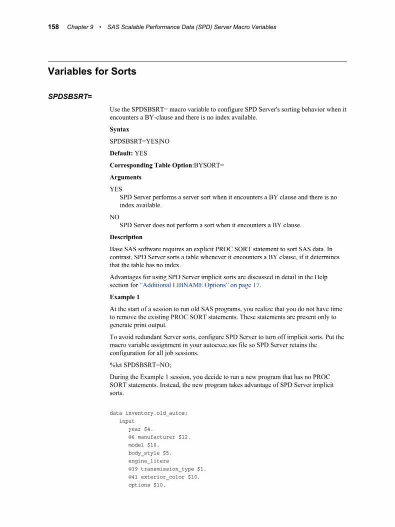
Variables for Sorts
SPDSBSRT=Use the SPDSBSRT= macro variable to configure SPD Server's sorting behavior when it encounters a BY-clause and there is no index available.
Syntax
SPDSBSRT=YES|NO
Default: YES
Corresponding Table Option:BYSORT=
Arguments
YESSPD Server performs a server sort when it encounters a BY clause and there is no index available.
NOSPD Server does not perform a sort when it encounters a BY clause.
Description
Base SAS software requires an explicit PROC SORT statement to sort SAS data. In contrast, SPD Server sorts a table whenever it encounters a BY clause, if it determines that the table has no index.
Advantages for using SPD Server implicit sorts are discussed in detail in the Help section for “Additional LIBNAME Options” on page 17.
Example 1
At the start of a session to run old SAS programs, you realize that you do not have time to remove the existing PROC SORT statements. These statements are present only to generate print output.
To avoid redundant Server sorts, configure SPD Server to turn off implicit sorts. Put the macro variable assignment in your autoexec.sas file so SPD Server retains the configuration for all job sessions.
%let SPDSBSRT=NO;
During the Example 1 session, you decide to run a new program that has no PROC SORT statements. Instead, the new program takes advantage of SPD Server implicit sorts.
data inventory.old_autos; input year $4. @6 manufacturer $12. model $10. body_style $5. engine_liters @39 transmission_type $1. @41 exterior_color $10. options $10.
158 Chapter 9 • SAS Scalable Performance Data (SPD) Server Macro Variables

mileage condition;
datalines;
1971 Buick Skylark conv 5.8 A yellow 00000001 143000 21982 Ford Fiesta hatch 1.2 M silver 00000001 70000 31975 Lancia Beta 2door 1.8 M dk blue 00000010 80000 41966 Oldsmobile Toronado 2door 7.0 A black 11000010 110000 31969 Ford Mustang sptrf 7.1 M red 00000111 125000 3;
PROC PRINT data=inventory.old_autos; by model;
run;
When the code executes, the PRINT procedure returns an error message. What happened? SAS expected INVENTORY.OLDAUTOS to be sorted before it would generate print output. Since there is no PROC SORT statement -- and implicit sorts are still turned off -- the sort does not occur.
Example 2
Keep implicit sorts turned off for the session, but specify an implicit sort for the table INVENTORY.OLDAUTOS.
PROC PRINT data=inventory.oldautos(bysort=yes); by model; run;
SPDSNBIX=Use the SPDSNBIX= macro variable to configure whether to use an index during a BY-sort.
Syntax
SPDSNBIX=YES|NO
Default: NO
Corresponding Server Parameter Option: [NO]BYINDEX
Arguments
YESSet SPDSNBIX=YES to suppress index use during a BY-sort. If the distribution of the values in the table are not relatively sorted or clustered, using the index for the BY sort can result in poor performance.
NOSet SPDSNBIX=NO or use the default value to allow the [NO]BYINDEX server parameter option to determine whether to use an index for a BY sort.
Example
%let SPDSNBIX=YES;
Variables for Sorts 159

SPDSSTAG=Use the SPDSSTAG= macro variable to specify whether to use non-tagged or tagged sorting for PROC SORT or BY processing.
Syntax
SPDSSTAG=YES|NO
Default: NO
Arguments
YESperforms tagged sorting.
NOperforms non-tagged sorting.
Description
During a non-tagged sort, SPD Server attaches the entire table column to the key field(s) to be sorted. Non-tagged sorting allows the software to deliver better performance than a tagged sort. Non-tagged sorting also requires more temporary disk space than a tagged sort.
Example
You are running low on disk space and you do not know whether you have enough disk overhead to accommodate the extra sort space required to support a non-tagged sort operation.
Configure SPD Server to perform a tagged sort.
%let SPDSSTAG=YES;
Variables for WHERE Clause Evaluations
SPDSTCNT=Use the SPDSTCNT= macro variable to specify the number of threads that you want to use during WHERE clause evaluations.
Syntax
SPDSTCNT=n
Default: The value of MAXWHTHREADS is configured by SPD Server parameters.
Used in Conjunction with the SPD Server Parameter: MAXWHTHREADS
Corresponding Table Option: THREADNUM=
Arguments
nis the number of threads.
Description
160 Chapter 9 • SAS Scalable Performance Data (SPD) Server Macro Variables

See “THREADNUM=” on page 204 for a description and an explanation of how SPDSTCNT= interacts with the SPD Server parameter MAXWHTHREADS.
SPDSEV1T=Use the SPDSEV1T= macro variable to indicate whether data returned from an SPD Server WHERE clause evaluations should be in strict row (observation) order.
The macro variables SPDSEV1T= and SPDSEV2T= work in conjunction with the SPD Server WHERE clause planner WHINIT.
The variables SPDSEV1T= and SPDSEV2T= are identical in purpose. You use them to specify the row order of data returned in WHERE-processing. Which variable the server exercises depends on the evaluation strategy selected by WHINIT. The SPDSEV1T= evaluation strategy is indexed. The SPDSEV2T= evaluation strategy is non-indexed. Avoid using these options unless you absolutely understand the SPD Server performance tradeoffs that depend on maintaining the order of data.
If compatibility with Base SAS software is important, set both SPDSEV1T= and SPDSEV2T= to 0. When both evaluation strategies are set to 0, SPD Server returns data in row order whether the SPDSEV1T= or the SPDSEV2T= strategy is selected.
When you use a SAS PROC to retrieve rows from a sorted table, some SAS PROCs can use the sort order information to optimize how to receive and process the rows. For example, if you use PROC SQL to perform table joins on a sorted table that uses WHERE predicates to filter table rows, then PROC SQL will use the sort order information to optimize the join strategy. If you use the default values of SPDSEV1T= and SPDSEV2T= in these instances, the SAS PROC receives the table rows in sorted order.
If the SAS PROC that you submit does not use the sorted order, the default values of SPDSEV1T= and SPDSEV2T= will restrict the use of parallel WHERE clauses, which can negatively impact performance. For example, PROC PRINT and most SAS DATA step code does not take advantage of sorted tables. If you know that the SAS PROC that you are submitting does not take advantage of a sorted table, you can change the setting for SPDSEV1T= or SPDSEV2T= to 2, in order to allow parallel WHERE evaluations that can improve performance. However, this should be done with care: a parallel WHERE evaluation does not guarantee that rows are returned to SAS in sorted order, and this can cause incorrect results for a SAS PROC that uses that information.
Note: The SPDSEV1T= and SPDSEV2T= usage that is discussed here does not apply to SQL statements that are executed via the SPD Server pass-through SQL facility.
Syntax
SPDSEV1T=0|1|2
Default: 1
Used in Conjunction with Indexed WHERE clause Evaluation Strategy
Arguments
0returns data in row order.
1might not return the data in row order. SPD Server can override as needed to force a 0 setting if the table is sorted using PROC SORT.
Variables for WHERE Clause Evaluations 161

2always forces parallel evaluation regardless of sorted order. May not return data in row order.
Description
If SPD Server must return many rows during WHERE clause processing, setting the variable to 0 will greatly slow performance. Use 0 only when row order is required. Use 2 only when you know row order is not important to the result.
Example
Configure SPD Server to send back data in row order whenever WHINIT performs an EVAL1 evaluation.
%let SPDSEV1T=0;
SPDSEV2T=Use the SPDSEV2T= macro variable to specify whether the data returned from WHERE clause evaluations should be in strict row (observation) order.
The macro variables SPDSEV1T= and SPDSEV2T= work in conjunction with the SPD Server WHERE clause planner WHINIT.
The variables SPDSEV1T= and SPDSEV2T= are identical in purpose. You use them to specify the row order of data returned in WHERE-processing. Which variable the server exercises depends on the evaluation strategy selected by WHINIT. The SPDSEV1T= evaluation strategy is indexed. The SPDSEV2T= evaluation strategy is non-indexed. Avoid using these options unless you absolutely understand the SPD Server performance tradeoffs that depend on maintaining the order of data.
If compatibility with Base SAS software is important, set both SPDSEV1T= and SPDSEV2T= to 0. When both evaluation strategies are set to 0, SPD Server returns data in row order whether the SPDSEV1T= or the SPDSEV2T= strategy is selected.
When you use a SAS PROC to retrieve rows from a sorted table, some SAS PROCs can use the sort order information to optimize how to receive and process the rows. For example, if you use PROC SQL to perform table joins on a sorted table that uses WHERE predicates to filter table rows, then PROC SQL will use the sort order information to optimize the join strategy. If you use the default values of SPDSEV1T= and SPDSEV2T= in these instances, the SAS PROC receives the table rows in sorted order.
If the SAS PROC that you submit does not use the sorted order, the default values of SPDSEV1T= and SPDSEV2T= will restrict the use of parallel WHERE clauses, which can negatively impact performance. For example, PROC PRINT and most SAS DATA step code does not take advantage of sorted tables. If you know that the SAS PROC that you are submitting does not take advantage of a sorted table, you can change the setting for SPDSEV1T= or SPDSEV2T= to 2, in order to allow parallel WHERE evaluations that can improve performance. However, this should be done with care: a parallel WHERE evaluation does not guarantee that rows are returned to SAS in sorted order, and this can cause incorrect results for a SAS PROC that uses that information.
Note: The SPDSEV1T= and SPDSEV2T= usage that is discussed here does not apply to SQL statements that are executed via the SPD Server pass-through SQL facility.
Syntax
SPDSEV2T=0|1|2
Default: 1
162 Chapter 9 • SAS Scalable Performance Data (SPD) Server Macro Variables

Used in Conjunction with Non-Indexed WHERE clause Evaluation Strategy
Arguments
0returns data in row order.
1might not return the data in row order. SPD Server can override as needed to force 0 setting if the table is sorted using PROC SORT.
2always forces parallel evaluation regardless of sorted order. May not return the data in row order.
Description
If SPD Server must return many rows during WHERE clause processing, setting the variable to 0 will greatly slow performance. Use 0 only when row order is required. Use 2 only when you know row order is not important to the result.
Example
Configure SPD Server to send back data in row order whenever WHINIT performs an EVAL2 evaluation.
%let SPDSEV2T=0;
SPDSWDEB=Use the SPDSWDEB= macro variable to specify whether the WHERE clause planner WHINIT, when evaluating a WHERE expression, should display a summary of the execution plan.
Syntax
SPDSWDEB=YES|NO
Default: NO
Arguments
YESdisplays WHINIT's planning output.
NOsuppresses WHINIT's planning output.
SPDSIRAT=Use the SPDSIRAT= macro variables to specify whether to perform segment candidate pre-evaluation when performing WHERE clause processing with hybrid indexes.
Syntax
SPDSIRAT=0..100
Default: MAXSEGRATIO server parameter
Description:
When using hybrid indexes, WHERE-based queries pre-evaluate segments. The segments are scanned for candidates that match one or more predicates in the WHERE clause. The candidate segments that were identified during the pre-evaluation are
Variables for WHERE Clause Evaluations 163

queried in subsequent logic to evaluate the WHERE clause. Eliminating the non-candidate segments from the WHERE clause evaluation generally results in substantial performance gains.
Some queries can benefit by limiting the pre-evaluation phase. SPD Server imposes the limit based on a ratio: the number of segments that contain candidates compared to the total number of segments in the table. The reason for this is simple. If the predicate has candidates in a high percentage of the segments, the pre-evaluation work is largely wasted.
The ratio formed by dividing the number of segments that containing candidates by the number of total segments is compared to a cutoff point. If the segment ratio is greater than the value assigned to the cutoff point, the extra processing required to perform pre-evaluation outweighs any potential process savings that might be gained through the predicate pre-evaluation. SPD Server calculates the ratio for a given predicate and compares the ratio to the SPDSIRAT= value, which acts as the cutoff point. If the calculated ratio is less than or equal to the SPDSIRAT= value, pre-evaluation is performed. If the calculated ratio is greater than the SPDSIRAT= value, pre-evaluation is skipped and every segment is a candidate for the WHERE clause.
Use the global SPD Server parameter, MAXSEGRATIO to set the default cutoff value. The default MAXSEGRATIO should provide good performance. Certain specific query situations might be justification for modifying your SPDSIRAT= value. When you modify your SPDSIRAT= value, it overrides the default value established by MAXSEGRATIO.
Example:
Configure SPD Server to perform a pre-evaluation phase for WHERE clause processing with hybrid indexes if the candidates are in 65% or less of the segments.
%let SPDSIRAT=65;
SPDSNIDX=Use the SPDSNIDX= macro variable to specify whether to use the table's indexes when processing WHERE clauses. SPDSNIDX= can also be used to disable index use for BY- order determination.
Syntax
SPDSNIDX=YES|NO
Default: NO
Corresponding Table Option: NOINDEX=
Arguments
YESignores indexes when processing WHERE clauses.
NOuses indexes when processing WHERE clauses.
Description:
Set SPDSNIDX=YES to test the effect of indexes on performance or for specific processing. Do not use YES routinely for normal processing.
Example:
164 Chapter 9 • SAS Scalable Performance Data (SPD) Server Macro Variables

Assume you are processing data from SPORT.MAILLIST. There is an index for the SEX column, and you should test it to determine whether the index will improve performance when you use PROC PRINT processing on SPORT.MAILLIST.
You should configure SPD Server not to use the index:
data sport.maillist; input name $ 1-20 address $ 21-57 phoneno $ 58-69 sex $71;
datalines;
Douglas, Mike 3256 Main St., Cary, NC 27511 919-444-5555 MWalters, Ann Marie 256 Evans Dr., Durham, NC 27707 919-324-6786 FTurner, Julia 709 Cedar Rd., Cary, NC 27513 919-555-9045 FCashwell, Jack 567 Scott Ln., Chapel Hill, NC 27514 919-533-3845 MClark, John 9 Church St., Durham, NC 27705 919-324-0390 M;
PROC DATASETS lib=sport nolist;modify maillist;index create sex;quit;
/*Turn on the macro variable SPDSWDEB *//* to show that the index is not used *//* during the table processing. */
%let spdswdeb=YES;
%let spdsnidx=YES;
title "All Females from Current Mailing List";PROC PRINT data=sport.maillist;where sex="F";run;
%let spdsnidx=NO;
SPDSWCST=Use the SPDSWCST= macro variable to specify whether to use dynamic WHERE clause costing.
Syntax
SPDSWCST=YES|NO
Default: NO
Corresponding Server Parameter Option: [NO]WHERECOSTING
Turns WHERE-costing on or off for an entire server.
Description:
Variables for WHERE Clause Evaluations 165

Set SPDSWCST=YES to use dynamic WHERE clause costing. Disabling SPDSWCST= defaults SPD Server to using WHERE-costing with WHINIT.
Example:
%let SPDSWCST=YES;
SPDSWSEQ=Syntax
SPDSWSEQ=YES|NO
Default: NO
Description:
Set the SPDSWSEQ= macro variable to YES. When set to YES, the SPDSWSEQ= macro variable overrides WHERE clause costing and forces a global EVAL3 or EVAL4 strategy.
Example:
%let SPDSWSEQ=YES;
Variables That Affect Disk Space
SPDSCMPF=Use the SPDSCMPF= macro variable to specify the amount of growth space, sized in bytes, to be added to a compressed data block.
Syntax
SPDSCMPF=n
Default: 0 bytes
Arguments
nis the number of bytes to add.
Description
Updating rows in compressed tables can increase the size of a given table block. Additional space is required for the block to be written back to disk. When contiguous space is not available on the hard drive, a new block fragment stores the excess, updated quantity. Over time, the table will experience block fragmentation.
When opening compressed tables for OUTPUT or UPDATE, you can use the SPDSCMPF= macro variable to anticipate growth space for the table blocks. If you estimate correctly, you can greatly reduce block fragmentation in the table.
Note: SPD Server table metadata does not retain compression buffer or growth space settings.
166 Chapter 9 • SAS Scalable Performance Data (SPD) Server Macro Variables

SPDSDCMP=Use the SPDSDCMP= macro variable to compress SPD Server tables that are stored on disk.
Syntax
SPDSDCMP=YES|NO|BINARY
Default: NO
Use in Conjunction with Table Option: IOBLOCKSIZE=
Corresponding Table Option: COMPRESS=
Arguments
YESperforms run-length compression on character data.
NOperforms no table compression.
BINARYperforms character and numeric compression.
Description
When you set the SPDSDCMP= macro variable to YES, SPD Server compresses newly created tables by 'blocks' according to the algorithm specified. To control the amount of compression, use the table option IOBLOCKSIZE= to specify the number of rows that you want to store in the block. For a complete discussion, refer to “IOBLOCKSIZE=” on page 198.
Note: Once a compressed table is created, you cannot change its block size. To resize the block, you must PROC COPY the table to a new table, setting IOBLOCKSIZE= to the new block size for the output table.
Example
You should conserve disk space before you create a huge table. You can use SPDSCMP to compress character and numeric data at the beginning of your job.
%let SPDSDCMP=BINARY;
SPDSIASY=Use the SPDSIASY= macro variable to specify whether to create indexes in parallel when creating multiple indexes on an SPD Server table.
Syntax
SPDSIASY=YES|NO
Default: NO
Corresponding Table Option : ASYNCINDEX=
Arguments
YEScreates the indexes in parallel.
Variables That Affect Disk Space 167

NOcreates one index at a time.
Description
You use the macro variable SPDSIASY= to choose between parallel and sequential index creation on SPD Server tables with more than one index. One advantage of creating multiple indexes in parallel is speed. The speed enhancements that can be achieved with parallel indexes are not free. Parallel indexes require significantly more disk space for working storage. The default SPD Server setting for the SPDSIASY= macro variable is set to NO, in order to avoid exhausting the available work storage space.
However, if you have adequate disk space to support parallel sorts, it is strongly recommended that you override the default SPDSIASY=NO setting and assign SPDSIASY=YES. You can substantially increase performance -- indexes that take hours to build complete much faster.
How many indexes should you create in parallel? The answer depends on several factors, such as the number of CPUs in the SMP configuration and available storage space needed for index key sorting.
When managing disk space on your SPD Server, remember that grouping index create statements can minimize the number of table scans that SPD Server performs, but it also affects disk space consumption. There is an inverse relationship between the table scan frequency and disk space requirements. A minimal number of table scans requires more auxiliary disk space; a maximum number of table scans requires less auxiliary disk space.
Example
You perform batch processing from midnight to 6:00 a.m. All of your processing must be completed before start of the next work day. One frequently repeated batch job creates large indexes on a table, and usually takes several hours to complete. Configure SPD Server to create indexes in parallel to reduce the processing time.
%let SPDSIASY=YES;proc datasets lib=spds; modify a; index create x; index create y; modify a; index create comp=(x y) comp2=(y x); quit;
In the example above, the X and Y indexes will be created in parallel. After creating X and Y indexes, SPD Server creates the COMP and COMP2 indexes in parallel. In this example, two table scans are required: one table scan for the X and Y indexes, and a second table scan for the COMP and COMP2 indexes.
SPDSSIZE=Use the SPDSSIZE= macro variable to specify the size of an SPD Server table partition.
Syntax
SPDSSIZE=n
Default: 16 Megabytes
168 Chapter 9 • SAS Scalable Performance Data (SPD) Server Macro Variables

Corresponding Table Option: PARTSIZE=
Affected by LIBNAME option: DATAPATH=
Arguments
nis the size of the partition in Megabytes.
Description
Use this SPDSSIZE= macro variable option to improve performance of WHERE clause evaluation on non-indexed table columns.
Splitting the data portion of a server table at fixed-sized intervals allows SPD Server to introduce a high degree of scalability for non-indexed WHERE clause evaluation. This is because SPD Server launches threads in parallel and can evaluate different partitions of the table without file access or thread contention. The speed enhancement comes at the cost of disk usage. The more data table splits you create, the more you increase the number of files, which are required to store the rows of the table.
Scalability limits on the SPDSSIZE= macro variable ultimately depend on how you structure the DATAPATH= option in your LIBNAME statement. The configuration of the DATAPATH= file systems across striped volumes is important. You should spread each individual volume's striping configuration across multiple disk controllers and SCSI channels in the disk storage array. Your configuration goal, at the hardware level, should be to maximize parallelism when performing data retrieval.
The SPDSSIZE= specification is also limited by MINPARTSIZE=, an SPD Server parameter maintained by the SPD Server administrator. MINPARTSIZE= ensures that an over-zealous SAS user cannot arbitrarily create small partitions, thereby generating an excessive number of physical files. The default for MINPARTSIZE= is 16 Mbytes.
Note: The SPDSSIZE= value for a table cannot be changed after the table is created. To change the SPDSSIZE=, you must PROC COPY the table and use a different SPDSSIZE= (or PARTSIZE=) option setting on the new (output) table.
For an example using the table option, see “PARTSIZE=” on page 196.
%let SPDSSIZE=32;
Variables to Enhance Performance
SPDSNETP=Use the SPDSNETP= macro variable to size buffers in server memory for the network data packet.
Syntax
SPDSNETP=size-of-packet
Default: 32K
Corresponding Table Option: “NETPACKSIZE=” on page 199
Arguments
size-of-packetis the size (integer) in bytes of the network packet.
Variables to Enhance Performance 169
Description
When sizing the buffer for data packet transfer between SPD Server and your SAS client machine, the packet must be greater than or equal in size to one table row. See “NETPACKSIZE=” on page 199 for more information.
Example
Despite recent upgrades to your network connections, you are experiencing significant pauses when the SPD Server transfers data. You want to resize the data packet to send three rows at a time for a more continuous data flow.
Specify a buffer size in server memory that is three times the row size (6144 bytes.) Submit your SPDSNETP= macro variable statement at the top of your job.
%let SPDSNETP=18432;
SPDSSADD=Use the SPDSSADD= macro variable to specify whether SPD Server appends tables by transferring a single row at a time synchronously, or by transferring multiple rows asynchronously (block row appends).
Syntax
SPDSSADD=YES|NO
Default: NO
Related Table Option: SYNCADD=
Arguments
YESapplies a single row at a time during an Append operation. This behavior imitates the Base SAS engine.
NOappends multiple rows at a time
Description
SPDSSADD=YES slows performance. Use this argument only if you require strict compatibility with Base SAS software when processing a table. For a complete discussion, refer to “SYNCADD=” on page 194.
SPDSSYRD=Use the SPDSSYRD= macro variable to specify whether SPD Server should perform asynchronous data streaming when reading a table.
Syntax
SPDSSYRD=YES|NO
Default: NO
Related Table Option: SYNCREAD=
Arguments
YESenables asynchronous data streaming.
170 Chapter 9 • SAS Scalable Performance Data (SPD) Server Macro Variables

NOdisables asynchronous data streaming.
Description
Use SPDSSYRD=YES only with a MODIFY statement. If you use it with any other processing operation, you slow performance.
SPDSAUNQ=Use the SPDSAUNQ= macro variable setting to specify whether to cancel an append to a table if the table has a unique index and the append would violate the index uniqueness.
Syntax
SPDSAUNQ=YES|NO
Default: NO
Description:
Use SPDSAUNQ=YES macro variable to improve append performance to a table with unique indexes. If uniqueness is not maintained, the append is canceled and the table is returned to its state before the append. In such an instance, you can scrub the table to remove nonunique values and redo the append with the macro variable SPDSAUNQ= set to YES. The other alternative is to simply redo the append with the macro variable SPDSAUNQ= set to NO.
If SPDSAUNQ=NO, the SPD Server will enforce uniqueness at the expense of appending unique indexes in observation order one row at a time. If uniqueness is not maintained for any given row, that row is discarded from the append.
Variable for a Client and a Server Running on the Same UNIX Machine
SPDSCOMP=specifies to compress the data when sending a data packet through the network.
Syntax
SPDSCOMP=YES|NO
Default: NO
Variable for a Client and a Server Running on the Same UNIX Machine 171

172 Chapter 9 • SAS Scalable Performance Data (SPD) Server Macro Variables
Chapter 10
SAS Scalable Performance Data (SPD) Server LIBNAME Options
Introduction . . . . . . . . . . . . . . . . . . . . . . . . . . . . . . . . . . . . . . . . . . . . . . . . . . . . . . . . . 173
Options to Locate an SPD Server Host . . . . . . . . . . . . . . . . . . . . . . . . . . . . . . . . . . . 174HOST= . . . . . . . . . . . . . . . . . . . . . . . . . . . . . . . . . . . . . . . . . . . . . . . . . . . . . . . . . . 174SERVER= . . . . . . . . . . . . . . . . . . . . . . . . . . . . . . . . . . . . . . . . . . . . . . . . . . . . . . . . 175
Options to Identify the SPD Server Client . . . . . . . . . . . . . . . . . . . . . . . . . . . . . . . . 175ACLGRP= . . . . . . . . . . . . . . . . . . . . . . . . . . . . . . . . . . . . . . . . . . . . . . . . . . . . . . . 175AUTHDOMAIN= . . . . . . . . . . . . . . . . . . . . . . . . . . . . . . . . . . . . . . . . . . . . . . . . . 176CHNGPASS= . . . . . . . . . . . . . . . . . . . . . . . . . . . . . . . . . . . . . . . . . . . . . . . . . . . . . 177NEWPASSWORD= or NEWPASSWD= . . . . . . . . . . . . . . . . . . . . . . . . . . . . . . . 177PASSWORD= or PASSWD= . . . . . . . . . . . . . . . . . . . . . . . . . . . . . . . . . . . . . . . . 178PROMPT= . . . . . . . . . . . . . . . . . . . . . . . . . . . . . . . . . . . . . . . . . . . . . . . . . . . . . . . 179USER= . . . . . . . . . . . . . . . . . . . . . . . . . . . . . . . . . . . . . . . . . . . . . . . . . . . . . . . . . . 179
Options to Specify Implicit SQL Pass-Through . . . . . . . . . . . . . . . . . . . . . . . . . . . 180IP=YES . . . . . . . . . . . . . . . . . . . . . . . . . . . . . . . . . . . . . . . . . . . . . . . . . . . . . . . . . . 180PASSTHRU= . . . . . . . . . . . . . . . . . . . . . . . . . . . . . . . . . . . . . . . . . . . . . . . . . . . . . 180
Options for Access Control Lists (ACLs) . . . . . . . . . . . . . . . . . . . . . . . . . . . . . . . . . 181ACLSPECIAL= . . . . . . . . . . . . . . . . . . . . . . . . . . . . . . . . . . . . . . . . . . . . . . . . . . . 181
Options for a Client and Server Running on the Same UNIX Machine . . . . . . . . 182NETCOMP= . . . . . . . . . . . . . . . . . . . . . . . . . . . . . . . . . . . . . . . . . . . . . . . . . . . . . . 182
Options for Other Functions . . . . . . . . . . . . . . . . . . . . . . . . . . . . . . . . . . . . . . . . . . . 183BYSORT= . . . . . . . . . . . . . . . . . . . . . . . . . . . . . . . . . . . . . . . . . . . . . . . . . . . . . . . 183DISCONNECT= . . . . . . . . . . . . . . . . . . . . . . . . . . . . . . . . . . . . . . . . . . . . . . . . . . . 184ENDOBS= . . . . . . . . . . . . . . . . . . . . . . . . . . . . . . . . . . . . . . . . . . . . . . . . . . . . . . . 186LIBGEN= . . . . . . . . . . . . . . . . . . . . . . . . . . . . . . . . . . . . . . . . . . . . . . . . . . . . . . . . 187LOCKING= . . . . . . . . . . . . . . . . . . . . . . . . . . . . . . . . . . . . . . . . . . . . . . . . . . . . . . 188STARTOBS= . . . . . . . . . . . . . . . . . . . . . . . . . . . . . . . . . . . . . . . . . . . . . . . . . . . . . 190TEMP= . . . . . . . . . . . . . . . . . . . . . . . . . . . . . . . . . . . . . . . . . . . . . . . . . . . . . . . . . . 190TRUNCWARN= . . . . . . . . . . . . . . . . . . . . . . . . . . . . . . . . . . . . . . . . . . . . . . . . . . 191
IntroductionThis chapter contains reference information for the SPD Server LIBNAME options. The options are grouped by the function or purpose of their default value. You can change the default, thereby controlling how they function in different data situations. The examples for using the options assume that a LIBNAME statement to access the SPD Server engine SASSPDS has previously been issued.
173

When using the options, remember that if a table option is used subsequent to a LIBNAME option of the same name, the value of the table option or macro variable takes precedence.
Options to Locate an SPD Server Host
HOST=
SummarySpecifies an SPD Server machine by node name or IP address, and locates the Name Server using the SERVICE value.
SyntaxHOST=hostname <SERVICE=service>
Arguments
hostnameis the node name of the SPD Server machine or an IP address.
serviceis the name of a service or the port number for the SPD Server's Name Server.
DescriptionThis option provides the node name of an SPD Server host machine and locates the port number of the SPD Server's Name Server. When there is no SERVICE= specification, SPD Server checks the client's /etc/services file (or its equivalent file) for SPDSNAME – a reserved name for the SPD Server's Name Server.
ExamplesSpecify the server machine SAMSON and use the default named service SPDSNAME to obtain the port number of the SPD Server Name Server.
LIBNAME mylib sasspds 'spdsdata' host='samson';
Specify the server machine SAMSON and provide the port number of the SPD Server Name Server.
LIBNAME mylib sasspds 'spdsdata' host='samson' service='5002';
Using a Macro Variable to Specify the SPD Server HostAssign the macro variable SPDSHOST to the SPD Server host SAMSON so that the LIBNAME statement is not required to SAMSON.
%let spdshost=samson; LIBNAME mylib sasspds 'spdsdata'
174 Chapter 10 • SAS Scalable Performance Data (SPD) Server LIBNAME Options
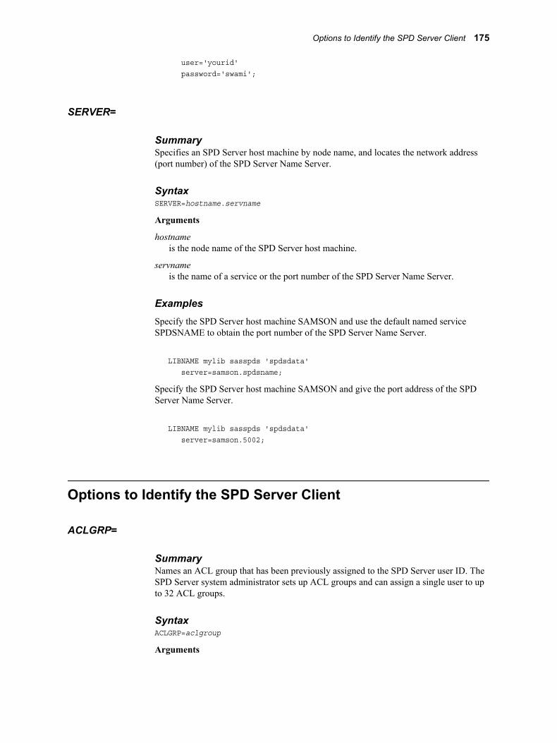
user='yourid' password='swami';
SERVER=
SummarySpecifies an SPD Server host machine by node name, and locates the network address (port number) of the SPD Server Name Server.
SyntaxSERVER=hostname.servname
Arguments
hostnameis the node name of the SPD Server host machine.
servnameis the name of a service or the port number of the SPD Server Name Server.
ExamplesSpecify the SPD Server host machine SAMSON and use the default named service SPDSNAME to obtain the port number of the SPD Server Name Server.
LIBNAME mylib sasspds 'spdsdata' server=samson.spdsname;
Specify the SPD Server host machine SAMSON and give the port address of the SPD Server Name Server.
LIBNAME mylib sasspds 'spdsdata' server=samson.5002;
Options to Identify the SPD Server Client
ACLGRP=
SummaryNames an ACL group that has been previously assigned to the SPD Server user ID. The SPD Server system administrator sets up ACL groups and can assign a single user to up to 32 ACL groups.
SyntaxACLGRP=aclgroup
Arguments
Options to Identify the SPD Server Client 175
aclgroupNames the ACL group that the SPD Server Administrator assigned to your SPD Server user ID. (You can be assigned up to five ACL groups.)
ExampleSpecify the ACL group PROD.
LIBNAME mylib sasspds 'spdsdata' user='receiver' aclgrp='PROD' prompt=yes;
Note: Password values are case sensitive. If the SPD Server administrator assigns a lowercase password value, you must enter the password value in lowercase.
AUTHDOMAIN=
SummaryAllows connection to a server by specifying the name of an authentication domain metadata object.
SyntaxAUTHDOMAIN=auth-domain
Arguments
auth-domainname of an authentication domain metadata object.
DetailsIf you specify AUTHDOMAIN=, you must specify SERVER=. However, the authentication domain references credentials so that you do not need to explicitly specify USER= and PASSWORD=.
The syntax is
AUTHDOMAIN=MyServerAuth
.
An administrator creates authentication domain definitions while creating a user definition with the User Manager in SAS Management Console. The authentication domain is associated with one or more login metadata objects that provide access to the server and is resolved by the DBMS engine calling the SAS Metadata Server and returning the authentication credentials.
The authentication domain and the associated login definition must be stored in a metadata repository and the metadata server must be running in order to resolve the metadata object specification.
Example
LIBNAME foo sasspds "spdsdata" host="hostname.na.companyname.com" serv="5400"
176 Chapter 10 • SAS Scalable Performance Data (SPD) Server LIBNAME Options
AUTHDOMAIN=spds;
CHNGPASS=
SummarySpecifies whether to prompt an SPD Server user for a change of password. If ACL file security is enabled, SPD Server validates the old and new password against its user ID table.
SyntaxCHNGPASS= YES | NO
Arguments
YESprompts for a change of the SPD Server user password.
NOsuppresses a prompt for a change of the SPD Server user password. This is the default.
ExampleSpecify a prompt to change the password of SPD Server user TEMPHIRE.
LIBNAME mylib sasspds 'spdsdata' user='temphire' password='whizbang' chngpass=yes;
Note: If you are using LDAP user authentication, and you create a user connection that uses the CHNGPASS= LIBNAME option, the user password will not be changed. If you are using LDAP authentication and want to change a user password, follow the operating system procedures to change a user password, and check with your LDAP server administrator to ensure that the LDAP database also records password changes.
NEWPASSWORD= or NEWPASSWD=
SummarySpecifies a new password for an SPD Server client user. If ACL file security is enabled, SPD Server validates the old or new password against its user ID table.
Syntax
NEWPASSWORD= newpasswordNEWPASSWD= newpassword
Arguments
newpasswordis the new password of an SPD Server client user. The password, visible in a SAS program, is encrypted in the SAS log file.
Options to Identify the SPD Server Client 177

ExampleSpecify a new password rambo for SPD Server client user RECEIVER.
LIBNAME mylib sasspds 'spdsdata' user='receiver' password='whizbang' newpassword='rambo';
Note: If you are using LDAP user authentication, and you create a user connection that uses the NEWPASSWORD= LIBNAME option, the user password will not be changed. If you are using LDAP authentication and want to change a user password, follow the operating system procedures to change a user password, and check with your LDAP server administrator to ensure that the LDAP database also records password changes.
PASSWORD= or PASSWD=
SummarySpecifies the SPD Server password of an SPD Server client user. If ACL file security is enabled, SPD Server validates the password against its user ID table.
Syntax
PASSWORD='password'PASSWD='password'
Arguments
'password'is the case-sensitive password of an SPD Server client user. The password, visible in a SAS program, is encrypted in the SAS log file.
ExampleSpecify the password whizbang for SPD Server client user SPDSUSER.
LIBNAME mylib sasspds 'spdsdata' server=kaboom.5200 user='spdsuser' password='whizbang';
OptionsSPD Server 5.1 supports SAS PROC PWENCODE. This permits scripts to be generated that do not explicitly contain secure passwords that could easily be used without authorization. You must run PROC PWENCODE in Base SAS to enable the usage of script password encoding within SPD Server 5.1. See the Base SAS documentation for detailed instruction on running PROC PWENCODE for use with SPD Server 5.1.
The example below shows an SPD Server LIBNAME statement that uses the password encoding option:
LIBNAME mylib sasspds 'spdsdata' server=kaboom.5200 user='spdsuser'
178 Chapter 10 • SAS Scalable Performance Data (SPD) Server LIBNAME Options

password='{sas001}c3BkczEyMw==';
PROMPT=
SummarySpecifies whether to prompt an SPD Server user for a password. If ACL file security is enabled, SPD Server validates the password against its user ID table.
SyntaxPROMPT= YES | NO
Arguments
YESprompts an SPD Server user for a password.
NOsuppresses a prompt for a password.
ExampleConfigure SPD Server to prompt SPD Server user BIGWHIG for a password.
LIBNAME mylib sasspds 'spdsdata' user='bigwhig' prompt=yes;
USER=
SummarySpecifies the ID of an SPD Server client user. If ACL file security is enabled, SPD Server validates the ID against its user ID table. (The SPD Server user ID defaults to the SAS process user ID if it is available, that is, when the client is not a Windows client.)
SyntaxUSER='username'
Arguments
'username'is the ID of an SPD Server client user.
ExampleSpecify the identifier SPDSUSER for an SPD Server client user.
LIBNAME mylib sasspds 'spdsdata' user='spdsuser' prompt=yes;
Options to Identify the SPD Server Client 179

Options to Specify Implicit SQL Pass-Through
IP=YES
SummaryThis is an abbreviated specification which replaces the more verbose PASSTHRU= option. The IP=YES option draws on information specified in the LIBNAME declaration. The IP=YES option specifies an implicit SQL pass-through connection for a single user to a specified domain and server during a given SPD Server session.
Syntax
LIBNAME BOAF sasspds 'BOAF' server=kaboom.5200 user='rcnye' password='*******' IP=YES ;
PASSTHRU=
SummaryThis older and more verbose specification for IP=YES is still supported. It specifies an implicit SQL pass-through connection for a single user to a specified domain and server during a given SPD Server session.
Syntax
PASSTHRU=<'dbq=<SAS-data-library> <SPD Server-options> user=<'UserID'> password=<'password'> ;
Arguments
DBQ=libname-domain (required)Specifies the primary SPD Server LIBNAME domain for the SQL pass-through connection. The name that you specify is identical to the LIBNAME domain name that you used when making a SAS LIBNAME assignment to sasspds. Use single or double quotes around the specified value.
SPD Server-optionsone or more SPD Server options.
USER=SPD Server user ID (required on Windows, but not UNIX)Specifies an SPD Server user ID in order to access an SPD Server SQL Server. Use single or double quotes around the specified value.
PASSWORD=password (required, or use PROMPT=YES, unless USER='anonymous')Specifies an SPD Server user ID password to access an SPD Server. (This value is case sensitive.)
180 Chapter 10 • SAS Scalable Performance Data (SPD) Server LIBNAME Options
Example:The following is a LIBNAME statement that specifies the implicit SQL pass-through option for user rcnye, using a libref to connect to the domain named 'BOAF' on the server named 'Kaboom' on port 5200:
LIBNAME BOAF sasspds 'BOAF' server=kaboom.5200 user='rcnye' password='*******'
PASSTHRU=' dbq="BOAF" server=kaboom.5200 user="rcnye" password="*******"' ;
OptionsSPD Server 5.1 supports SAS PROC PWENCODE. This permits scripts to be generated that do not explicitly contain secure passwords that could easily be used without authorization. You must run PROC PWENCODE in Base SAS to enable the usage of script password encoding within SPD Server 5.1. See the Base SAS documentation for detailed instruction on running PROC PWENCODE with SPD Server 5.1.
The example below shows an SPD Server LIBNAME statement that uses the password encoding option:
LIBNAME mylib sasspds 'spdsdata' server=kaboom.5200 user='spdsuser' password='{sas001}c3BkczEyMw=='
PASSTHRU=' dbq="spdsdata" server=kaboom.5200 user="spdsuser" password="{sas001}c3BkczEyMw=="';
Options for Access Control Lists (ACLs)
ACLSPECIAL=
SummaryGrants special access to SPD Server resources in the LIBNAME domain to an SPD Server user. The SPD Server user must also be defined as 'special' by the SPD Server administrator.
SyntaxACLSPECIAL=YES | NO
Arguments
Options for Access Control Lists (ACLs) 181

YESgrants special access (Read, Write, Alter, and Control permission) to all SPD Server resources in the domain.
NOdenies special access (Read, Write, Alter, and Control permission) to all SPD Server resources in the domain.
DescriptionGrants special privileges to all SPD Server tables and associated indexes in the LIBNAME domain. The special privileges, (Read, Write, Alter, and Control permission), override normal ACL restrictions only if the SPD Server administrator defines the user as 'special' in the user ID table.
ExampleGrant special privileges to THEBOSS allowing him to Read, Write, Alter, and Control all tables in the CONVERSION_AREA domain. (The SPD Server administrator has defined THEBOSS as 'special'.)
LIBNAME mydatalib sasspds 'conversion_area' server=husky.5105 user='theboss' prompt=yes aclspecial=yes ;
Options for a Client and Server Running on the Same UNIX Machine
NETCOMP=
SummaryCompresses the data stream for an SPD Server network packet.
SyntaxNETCOMP=YES | NO
Arguments
YESsends compressed data in an SPD Server network packet.
NOsends uncompressed data in an SPD Server network packet.
DescriptionNormally, data compression for inter-process transfers is recommended. However, for a client and server process on the same machine -- with UNIXDOMAIN=YES -- turning off compression can improve performance. You should examine NETCOMP together with UNIXDOMAIN and NETPACKSIZE for both client and server on the same machine.
182 Chapter 10 • SAS Scalable Performance Data (SPD) Server LIBNAME Options
ExampleSpecify to turn off compression of the data stream.
LIBNAME mylib sasspds 'test_area' netcomp=no;
Options for Other Functions
BYSORT=
SummarySpecifies whether to use implicit automatic SPD Server sorts on BY clauses.
SyntaxBYSORT=YES | NO
Arguments
YESperforms an implicit sort for a BY clause. This is the default.
NOdoes not perform an implicit sort for a BY clause.
DescriptionWhere Base SAS software requires an explicit sort statement (PROC SORT) to sort SAS data, by default, SPD Server performs a sort whenever it encounters a BY clause. If the value of the BYSORT= option is NO, the SPD Server software performs the same as the Base SAS engine.
Example 1Specify to turn off implicit SPD Server sorts for the session.
LIBNAME mydatalib sasspds 'conversion_area' server=husky.5105 user='siteusr1' prompt=yes bysort=no ;
data mydatalib.old_autos; input year $4. @6 manufacturer $12. model $10. body_style $5. engine_liters @39 transmission_type $1. @41 exterior_color $10. options $10. mileage condition ;
Options for Other Functions 183

datalines ;
1971 Buick Skylark conv 5.8 A yellow 00000001 143000 21982 Ford Fiesta hatch 1.2 M silver 00000001 70000 31975 Lancia Beta 2door 1.8 M dk blue 00000010 80000 41966 Oldsmobile Toronado 2door 7.0 A black 11000010 110000 31969 Ford Mustang sptrf 7.1 M red 00000111 125000 3;
PROC PRINT data=mydatalib.old_autos; by model;run;
In this program, the PRINT procedure will return an error message because the table MYDATALIB.OLD_AUTOS is not sorted.
Example 2Turn off implicit SPD Server sorts with the LIBNAME option, but specify a server sort for the table MYDATALIB.OLD_AUTOS using the BYSORT table option.
PROC PRINT data=mydatalib.old_autos (bysort=yes); by model;run;
DISCONNECT=
SummaryThe DISCONNECT= option is used to control how user proxy resources are assigned for an SPD Server user. Each SPD Server user in a SAS session requires an SPD Server user proxy process to handles client requests.
SyntaxDISCONNECT=YES | NO
Arguments
YEScloses network connections between the SAS client and SPD Server when all SPD Server librefs are cleared.
NOcloses network connections between the SAS client and SPD Server only when the SAS session ends. This is the default setting.
DescriptionThe DISCONNECT= option is used to control how user proxy resources are created and terminated for an SPD Server user. Each SPD Server user in a SAS session requires an SPD Server user proxy process to handles client requests.
The DISCONNECT= state of the user proxy is determined by the first LIBNAME statement a user issues in the SAS session.
When the DISCONNECT= option is set to NO, the network connections between the SAS client and the SPD Server user proxy are closed when the SAS session ends.
184 Chapter 10 • SAS Scalable Performance Data (SPD) Server LIBNAME Options

Closing the network connection ends all SPD Server user proxy processes for that session.
When the DISCONNECT= option is set to YES, the network connections between the SAS client and the SPD Server user proxy are closed after the user's last SPD Server libref in the SAS session is cleared. Closing the network connection ends all SPD Server user proxy processes, but not necessarily the SAS session. If the user issues a subsequent SPD Server libref in that SAS session, a new SPD Server user proxy process must be started up.
The advantage of using DISCONNECT=NO is that the processor overhead that is required to create an SPD Server user proxy is required only when an SPD Server user issues his first LIBNAME of his session. The disadvantage of using DISCONNECT=NO is that the SPD Server user proxy does not terminate until the user's SAS session ends. For example, if a user does not log off at the end of the day and leaves an SPD Server session running overnight, the user proxy remains in force, occupying system resources that might be used by other jobs.
The advantage of using DISCONNECT=YES is that user resources are freed as soon as the user's last LIBNAME of the session is cleared. The disadvantage of using DISCONNECT=YES is if the user needs to issue a subsequent LIBNAME in that session, the LIBNAME assignment will require a new SPD Server user proxy to be launched.
The DISCONNECT=YES LIBNAME option must be used with the LIBNAME CLEAR statement to be effective.
The default setting for the DISCONNECT= option is NO.
Example 1Use the default setting of DISCONNECT=NO to retain the user proxy process. Libref SPUD is assigned using user proxy process 8292, and then libref SPUD is cleared. Then libref CAKE is assigned, still using user proxy process 8292. The user proxy process is not terminated when libref SPUD is cleared, and no new user proxy process is required to assign libref CAKE.
LIBNAME spud sasspds 'potatoes' server=husky.6100 user='bob' passwd='bob123';
NOTE: Libref SPUD was successfully assigned as follows: Engine: SASSPDS Physical Name: :8292/spds/test/potatoes/
LIBNAME spud clear;
LIBNAME cake sasspds 'carrots' server=husky.6100 user='bob' passwd='bob123';
NOTE: Libref CAKE was successfully assigned as follows: Engine: SASSPDS Physical Name: :8292/spds/test/carrots/
Options for Other Functions 185

Example 2Use the DISCONNECT=YES setting to terminate the user proxy process when the last user LIBNAME is cleared. Libref SPUD is user Bob's last open LIBNAME. SPUD is assigned using user proxy process 8234, and then cleared. Next, libref CAKE is assigned using user proxy process 8240. When libref SPUD is cleared, user proxy process 8234 is terminated, and the resources that were allocated to proxy process 8324 are freed. When Bob submits a subsequent libref statement for CAKE, a new user proxy process 8240 is created.
LIBNAME spud sasspds 'potatoes' server=husky.6100 user='bob' passwd='bob123'DISCONNECT=YES;
NOTE: Libref SPUD was successfully assigned as follows: Engine: SASSPDS Physical Name: :8234/spds/test/potatoes/
LIBNAME spud clear;
LIBNAME cake sasspds 'carrots' server=husky.6100 user='bob' passwd='bob123'DISCONNECT=YES;
NOTE: Libref CAKE was successfully assigned as follows: Engine: SASSPDS Physical Name: :8240/spds/test/carrots/
Now Bob has libref CAKE assigned using user proxy process 8240. Suppose Bob makes another libref FRUIT without first clearing the CAKE libref. The libref FRUIT will re-use the active proxy process 8240. In this case, both the CAKE and FRUIT librefs must be cleared before the user proxy process can terminate.
LIBNAME fruit sasspds 'apples' server=husky.6100 user='bob' passwd='bob123'DISCONNECT=YES;
NOTE: Libref FRUIT was successfully assigned as follows: Engine: SASSPDS Physical Name: :8240/spds/test/apples/
ENDOBS=
SummarySpecifies the end row (observation) number in a user-defined range for processing.
SyntaxENDOBS=n
186 Chapter 10 • SAS Scalable Performance Data (SPD) Server LIBNAME Options
Arguments
nis the number of the end row.
DescriptionBy default SPD Server processes the entire table unless the user specifies a range of rows with the STARTOBS= and ENDOBS= options. If the STARTOBS= option is used without the ENDOBS= option, the implied value of ENDOBS= is the end of the table. When both options are used together, the value of ENDOBS= must be greater than STARTOBS=.
In contrast to the Base SAS software options FIRSTOBS= and OBS=, the STARTOBS= and ENDOBS= SPD Server options can be used for WHERE clause processing in addition to table input operations.
Example 1Specify for SPD Server to process only row numbers (observations) 200 - 500 while the LIBNAME is active.
LIBNAME mydatalib sasspds 'conversion_area' server=husky.5105 user='siteusr1' prompt=yes startobs=200 endobs=500;
LIBGEN=
SummaryThe LIBGEN=YES option is used in explicit SQL connection statements. When you set LIBGEN= yes, SPD Server is configured to generate additional domain connections that enable you to perform SQL joins across different SPD Server domains.
SyntaxLIBGEN=YES
DescriptionYou should specify the LIBGEN=YES option in the explicit SQL LIBNAME connection. You cannot specify the LIBGEN=YES option setting without first creating a LIBNAME connections to the domain.
ExamplesThe following example uses explicit SQL to join two tables from different domains. It uses the LIBGEN=YES option to perform the join without having to issue an extra execute connection statement.
SQL with LIBGEN=YES
/* The example code that uses LIBGEN=YES *//* can join the tables from two different */
Options for Other Functions 187

/* domains in a more simple manner. */
LIBNAME path1 sasspds 'path1' server=boxer.5140 LIBGEN=YES ip=YES user='anonymous' ;
LIBNAME path2 sasspds 'path2' server=boxer.5140 LIBGEN=YES ip=YES user='anonymous' ;
DATA path1.table1 (keep=i table1)path2.table2 (keep=i table2) ;
table1 = 'table1' ;table2 = 'table2' ;
do i = 1 to 10 ; output ; end ;run ;
PROC SQL ;CONNECT to sasspds ( dbq='Path1' server=boxer.5140 user='anonymous') ;
/* Syntax used with LIBGEN=YES option */
execute (create table table4 as select * from path1.table1 a, path2.table2 b where a.i = b.i)by sasspds ;
disconnect from sasspds ;
quit ;
LOCKING=
Overview of Record-Level LockingRecord-level locking is an SPD Server feature that allows multiple users concurrent Read and Write access to SPD Server tables while maintaining the integrity of the table contents. When record-level locking is enabled, users can insert, append, delete, and
188 Chapter 10 • SAS Scalable Performance Data (SPD) Server LIBNAME Options
update the contents of an SPD Server table while performing concurrent reads on the table. When a client enables record-level locking, the client connects to the single SPD Server record-level locking proxy process. When record-level locking is not enabled, clients connect to separate SPD Server user proxy processes for each LIBNAME connection to a domain.
Record-Level Locking DetailsRecord-level locking is enabled when an SPD Server client specifies the LOCKING=YES LIBNAME option to the client's LIBNAME connection statement. All subsequent operations on the given LIBNAME domain will use record-level locking. The primary use of record-level locking is to allow multiple clients or parallel operations from the same client to have both Read and Write access to the same SPD Server table resource. If record-level locking is not enabled, then any Write operation (update, append, insert, or delete) on an SPD Server table requires exclusive access to the resource, or a member lock failure error occurs. Operations that affect metadata, such as creating or deleting indexes, renaming variables, and renaming tables require exclusive access to the resource, whether record-level locking is enabled or not. These types of operations will report a member lock failure error when record-level locking is enabled, but exclusive access is not available.
Record-level locking must be enabled in SPD Server before a SAS client can use the CNTLEV=REC table option in their SAS program to access SPD Server tables. Record-level locking enforces SAS style record-level integrity across multiple clients so clients are guaranteed that an observation will not change during a multiphased Read or Write operation on the specified observation. Record-level locking will allow multiple concurrent update access to a single SPD Server table, but it will deny concurrent access to the specified observation within the table.
When an SPD Server client establishes a LIBNAME connection to a domain with record-level locking enabled, it connects using the single record-level locking proxy process. There is only one record-level locking proxy process per SPD Server. All SPD Server clients that use record-level locking connections are processed through the record-level locking proxy process. If there are a large number of record-level locking connections, there might be some contention for process resources between the clients. The record-level locking proxy process is a single point of failure for all these connections, so care should be taken when you use record-level locking to update critical data.
When you append or insert new rows into a table with defined indexes, the table updates are processed more sequentially through the record-level locking proxy process than they would be through the SPD Server user proxy processes. The performance of record-level locking will probably be less than the performance that can be obtained without record-level locking enabled for these types of operations. The standard member-level locking that is used in SPD Server user proxy processes allows for more parallel processing when doing table append or insert operations.
Record-level locking is not supported for operations on tables that use dynamic clusters.
SyntaxLOCKING=YES|NO
Default: NO
Arguments
YESenables record sharing mode.
Options for Other Functions 189

NOdisables record sharing mode.
Example
LIBNAME testrl sasspds 'tmp' server=serverNode.port user='anonymous' locking=YES ;
STARTOBS=
SummarySpecifies the start row (observation) number in a user-defined range for processing.
SyntaxSTARTOBS=n
Arguments
nis the number of the start row.
DescriptionBy default SPD Server processes the entire table unless the user specifies a range of rows with the options STARTOBS= and ENDOBS=. If the ENDOBS= option is used without the STARTOBS= option, the implied value of STARTOBS= is 1. When both options are used together, the value of STARTOBS= must be less than the value of ENDOBS.=
In contrast to the Base SAS software options FIRSTOBS= and OBS=, the STARTOBS= and ENDOBS= SPD Server options can be used for WHERE clause processing in addition to table input operations.
ExampleSpecify for SPD Server to process only row numbers (observations) 200–500 while the LIBNAME is active.
LIBNAME mydatalib sasspds 'conversion_area' server=husky.5105 user='siteusr1' prompt=yes startobs=200 endobs=500;
TEMP=
SummaryControls the creation of a temporary LIBNAME domain for this LIBNAME assignment.
190 Chapter 10 • SAS Scalable Performance Data (SPD) Server LIBNAME Options

SyntaxTEMP=YES|NO
Default: NO
Arguments
YEScreates a temporary LIBNAME domain for the LIBNAME assignment.
NOdoes not create a temporary LIBNAME domain.
DescriptionUse this option to create temporary LIBNAME domains that exist for the duration of the LIBNAME assignment. The TEMP (temporary) domains are analogous to SAS WORK libraries.
To create a temporary LIBNAME domain, use TEMP=YES. Any data objects, tables, catalogs, or utility files that are created in the TEMP=YES temporary domain are automatically deleted when you end the SAS session. This functions similarly to a SAS WORK library. (Note: The temporary domain is created as a subdirectory of the directory specified as the library domain.)
Example 1Create a LIBNAME domain to use for temporary storage during your SAS session.
LIBNAME mydatalib sasspds 'conversion_area' server=kaboom.5191 user='siteusr1' prompt=yes temp=yes ;
TRUNCWARN=
SummarySuppresses hard failure on NLS transcoding overflow and character mapping errors.
SyntaxTRUNCWARN=YES|NO
Default: NO
DescriptionWhen using the TRUNCWARN=YES LIBNAME option, data integrity might be compromised because significant characters can be lost in this configuration. The default setting is NO, which causes hard Read and Write stops when transcode overflow or mapping errors are encountered. When TRUNCWARN=YES, and an overflow or character mapping error occurs, a warning is posted to the SAS log at data set close time if overflow occurs, but the data overflow is lost.
Options for Other Functions 191

192 Chapter 10 • SAS Scalable Performance Data (SPD) Server LIBNAME Options
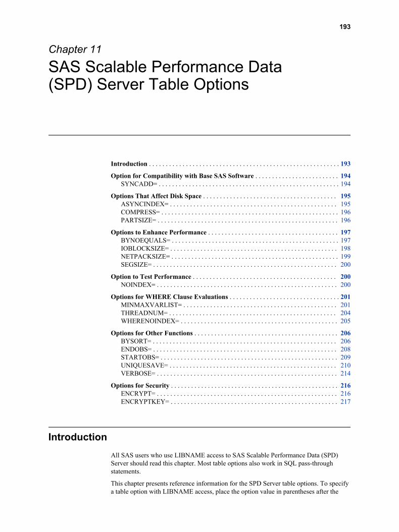
Chapter 11
SAS Scalable Performance Data (SPD) Server Table Options
Introduction . . . . . . . . . . . . . . . . . . . . . . . . . . . . . . . . . . . . . . . . . . . . . . . . . . . . . . . . . 193
Option for Compatibility with Base SAS Software . . . . . . . . . . . . . . . . . . . . . . . . . 194SYNCADD= . . . . . . . . . . . . . . . . . . . . . . . . . . . . . . . . . . . . . . . . . . . . . . . . . . . . . . 194
Options That Affect Disk Space . . . . . . . . . . . . . . . . . . . . . . . . . . . . . . . . . . . . . . . . 195ASYNCINDEX= . . . . . . . . . . . . . . . . . . . . . . . . . . . . . . . . . . . . . . . . . . . . . . . . . . 195COMPRESS= . . . . . . . . . . . . . . . . . . . . . . . . . . . . . . . . . . . . . . . . . . . . . . . . . . . . . 196PARTSIZE= . . . . . . . . . . . . . . . . . . . . . . . . . . . . . . . . . . . . . . . . . . . . . . . . . . . . . . 196
Options to Enhance Performance . . . . . . . . . . . . . . . . . . . . . . . . . . . . . . . . . . . . . . . 197BYNOEQUALS= . . . . . . . . . . . . . . . . . . . . . . . . . . . . . . . . . . . . . . . . . . . . . . . . . . 197IOBLOCKSIZE= . . . . . . . . . . . . . . . . . . . . . . . . . . . . . . . . . . . . . . . . . . . . . . . . . . 198NETPACKSIZE= . . . . . . . . . . . . . . . . . . . . . . . . . . . . . . . . . . . . . . . . . . . . . . . . . . 199SEGSIZE= . . . . . . . . . . . . . . . . . . . . . . . . . . . . . . . . . . . . . . . . . . . . . . . . . . . . . . . 200
Option to Test Performance . . . . . . . . . . . . . . . . . . . . . . . . . . . . . . . . . . . . . . . . . . . 200NOINDEX= . . . . . . . . . . . . . . . . . . . . . . . . . . . . . . . . . . . . . . . . . . . . . . . . . . . . . . 200
Options for WHERE Clause Evaluations . . . . . . . . . . . . . . . . . . . . . . . . . . . . . . . . . 201MINMAXVARLIST= . . . . . . . . . . . . . . . . . . . . . . . . . . . . . . . . . . . . . . . . . . . . . . 201THREADNUM= . . . . . . . . . . . . . . . . . . . . . . . . . . . . . . . . . . . . . . . . . . . . . . . . . . 204WHERENOINDEX= . . . . . . . . . . . . . . . . . . . . . . . . . . . . . . . . . . . . . . . . . . . . . . . 205
Options for Other Functions . . . . . . . . . . . . . . . . . . . . . . . . . . . . . . . . . . . . . . . . . . . 206BYSORT= . . . . . . . . . . . . . . . . . . . . . . . . . . . . . . . . . . . . . . . . . . . . . . . . . . . . . . . 206ENDOBS= . . . . . . . . . . . . . . . . . . . . . . . . . . . . . . . . . . . . . . . . . . . . . . . . . . . . . . . 208STARTOBS= . . . . . . . . . . . . . . . . . . . . . . . . . . . . . . . . . . . . . . . . . . . . . . . . . . . . . 209UNIQUESAVE= . . . . . . . . . . . . . . . . . . . . . . . . . . . . . . . . . . . . . . . . . . . . . . . . . . 210VERBOSE= . . . . . . . . . . . . . . . . . . . . . . . . . . . . . . . . . . . . . . . . . . . . . . . . . . . . . . 214
Options for Security . . . . . . . . . . . . . . . . . . . . . . . . . . . . . . . . . . . . . . . . . . . . . . . . . . 216ENCRYPT= . . . . . . . . . . . . . . . . . . . . . . . . . . . . . . . . . . . . . . . . . . . . . . . . . . . . . . 216ENCRYPTKEY= . . . . . . . . . . . . . . . . . . . . . . . . . . . . . . . . . . . . . . . . . . . . . . . . . . 217
IntroductionAll SAS users who use LIBNAME access to SAS Scalable Performance Data (SPD) Server should read this chapter. Most table options also work in SQL pass-through statements.
This chapter presents reference information for the SPD Server table options. To specify a table option with LIBNAME access, place the option value in parentheses after the
193
table name. The option value then specifies processing that applies only to that table. To specify a table option with pass-through access, place the option value in brackets after the table name. The option value then specifies processing that applies only to that table. The SPD Server table options that follow are grouped by the function of their default value.
When using the options in this chapter, remember that if a table option is used subsequent to a LIBNAME option or macro variable, the value of the table option takes precedence.
Option for Compatibility with Base SAS Software
SYNCADD=Specifies when appending to a table whether to apply a single or multiple rows at a time.
Syntax
SYNCADD=YES|NO
Default: NO
Corresponding Macro Variable
SPDSSADD
Related Table Option
UNIQUESAVE=
Arguments
YESimitates the behavior of the Base SAS engine, applying a single row at a time (synchronously).
NOappends multiple rows at a time (asynchronously).
Description
When SYNCADD= is set to YES, processing performance becomes slower. Use this setting only in order to force the server's append processing to be compatible with Base SAS software processing. That is, when the server encounters a row with a nonunique value, to cancel the Append operation, back out the transactions just added, and leave the original table on disk.
Example
In this example, when executing the first INSERT statement, PROC SQL permits insertion of the values 'rollback1' and 'rollback2' because the row additions to table A are performed asynchronously. PROC SQL does not get the true completion status at the time it adds a row.
When executing the second INSERT statement, PROC SQL performs a rollback on the INSERT, upon encountering the Add error on 'nonunique', and deletes the rows 'rollback3' and 'rollback4'.
data a; input z $ 1-20 x y;
194 Chapter 11 • SAS Scalable Performance Data (SPD) Server Table Options

list;
datalines;one 1 10two 2 20three 3 30four 4 40five 5 50;
PROC SQL sortseq=ascii exec noerrorstop;create unique index comp on a (x, y);insert into a values('rollback1', -80, -80) values('rollback2',-90, -90) values('nonunique', 2, 20);
insert into a(syncadd=yes) set z='rollback3', x=-60, y=-60 set z='rollback4', x=-70, y=-70 set z='nonunique', x=2, y=20; quit;
Options That Affect Disk Space
ASYNCINDEX=Specifies when creating multiple indexes on an SPD Server table whether to create the indexes in parallel.
Syntax
ASYNCINDEX=YES|NO
Default: NO
Corresponding Macro Variable
SPDSIASY
Arguments
YEScreates the indexes in parallel.
NOcreates a single index at a time.
Description
SPD Server can create multiple indexes for a table at the same time. To do this, it launches a single thread for each index created, and then processes the threads simultaneously. Although creating indexes in parallel is much faster, the default for this option is NO. The reason is because parallel creation requires additional sort work space that might not be available.
For a complete description of the benefits and tradeoffs of creating multiple indexes in parallel, see “SPDSIASY=” on page 167.
Options That Affect Disk Space 195

Example
Because the disk workspace required for parallel index creation is available, specify for SPD Server to create, in parallel, the X, Y, and COMP indexes for table A.
PROC DATASETS lib=mydatalib; modify a(asyncindex=yes); index create x; index create y; index create comp=(x y); quit;
COMPRESS=Compresses SPD Server tables on disk.
Syntax
COMPRESS=YES | NO | BINARY
Default: NO
Use in Conjunction with Table Option
IOBLOCKSIZE=
Corresponding Macro Variable
SPDSDCMP
Arguments
YESperforms the run-length compression algorithm SPDSRLLC.
NOperforms no table compression.
BINARYperforms both character and numeric data compression.
Description
When COMPRESS= is assigned YES, SPD Server compresses newly created tables by 'blocks' based on the algorithm specified. To control the amount of compression, use the table option IOBLOCKSIZE=. This option specifies the number of rows that you want to store in the block.
When COMPRESS=BINARY is specified, both numeric data and character data are compressed.
Note: Once a compressed table is created, you cannot change its block size. To resize the block, you must PROC COPY the table to a new table, setting IOBLOCKSIZE= to the block size desired for the output table.
PARTSIZE=Specifies the size of an SPD Server table partition.
Syntax
PARTSIZE=n
196 Chapter 11 • SAS Scalable Performance Data (SPD) Server Table Options

Default: 16 Megabytes
Corresponding Macro Variable
SPDSSIZE=
Arguments
nis the size of the partition in megabytes.
Description
Specifying PARTSIZE= forces the software to partition (split) SPD Server tables at the given size. The actual size is computed to accommodate the largest number of rows that will fit in the specified size of n Mbytes.
Use this option to improve performance of WHERE clause evaluation on non-indexed table columns and on SQL GROUP_BY processing. By splitting the data portion of a Scalable Platform Data Server table at fixed-sized intervals, the software can introduce a high degree of scalability for these operations. The reason: it can launch threads in parallel to perform the evaluation on different partitions of the table, without the threat of file access contention between the threads. There is, however, a price for the table splits: an increased number of files, which are required to store the rows of the table.
The PARTSIZE= specification is limited by MINPARTSIZE=, an SPD Server parameter maintained by the SPD Server administrator. MINPARTSIZE= ensures that an over-zealous SAS user does not create arbitrarily small partitions, thereby generating a large number of files. The default for MINPARTSIZE= is 16 Mbytes and probably should not be lowered much beyond this value.
Note: The PARTSIZE value for a table cannot be changed after a table is created. To change the PARTSIZE, you must PROC COPY the table and use a different PARTSIZE option setting on the new (output) table.
Example
Using PROC SQL, extract a set of rows from an existing table to create a non-indexed table with a partition size of 32 Mbytes in a SAS job:
PROC SQL;create table SPDSCEN.HR80SPDS(partsize=32) as select state, age, sex, hour89, industry, occup from SPDSCEN.PRECS where hour89 > 40;quit;
Options to Enhance Performance
BYNOEQUALS=Specifies the output order of table rows with identical values for the BY column.
Options to Enhance Performance 197
Syntax
BYNOEQUALS=YES | NO
Arguments
YESdoes not guarantee the output order of table rows with identical values in a BY clause.
NOguarantees the output order of table rows with identical values in a BY clause will be the relative table position of the rows from the input table. This is the default.
Example
Specify for SPD Server in the ensuing BY-column operation to output rows with identical values in the key column randomly.
data sport.racquets(index=(string)); input raqname $20. @22 weight @28 balance $2. @32 flex @36 gripsize @42 string $3. @47 price @55 instock; datalines;Solo Junior 10.1 N 2 3.75 syn 50.00 6Solo Lobber 11.3 N 10 5.5 syn 160.00 1Solo Queensize 10.9 HH 6 5.0 syn 130.00 3Solo Kingsize 13.1 HH 5 5.6 syn 140.00 3;
data sport.racqbal(bynoequal=yes); set sport.racquets; by balance;run;
IOBLOCKSIZE=Specifies the number of rows in a block to be stored in or read from an SPD Server table.
Syntax
IOBLOCKSIZE=n
Default: 4096
Use in Conjunction with Macro Variable “SPDSDCMP=” on page 167 or Table Options COMPRESS= or ENCRYPT= .
Arguments
nis the size of the block.
Description
198 Chapter 11 • SAS Scalable Performance Data (SPD) Server Table Options
The software reads and stores a server table in blocks. IOBLOCKSIZE= is useful on compressed or encrypted tables. SPD Server software does not use IOBLOCKSIZE= on noncompressed or nonencrypted tables.
For tables that you compress or encrypt, using either the option COMPRESS= or the macro variable SPDSDCMP=, the IOBLOCKSIZE= specification determines the number of rows to include in the block. The specification applies to block compression as well as data I/O to and from disk. The IOBLOCKSIZE= value affects the table's organization on disk.
When using SPD Server table compression or encryption, specify an IOBLOCKSIZE= value that complements how the data is to be accessed, sequentially or randomly. Sequential access or operations requiring full table scans favor a large block size, for example 64K. In contrast, random access favors a smaller block size, for example 8K.
Example
A huge company mailing list is processed sequentially. Specify a block size for compression that is optimal for sequential access.
/* IOblocksize set to 64K */data sport.maillist(ioblocksize=65536 compress=yes); input name $ 1-20 address $ 21-57 phoneno $ 58-69 sex $71;
datalines;
Douglas, Mike 3256 Main St., Cary, NC 27511 919-444-5555 MWalters, Ann Marie 256 Evans Dr., Durham, NC 27707 919-324-6786 FTurner, Julia 709 Cedar Rd., Cary, NC 27513 919-555-9045 FCashwell, Jack 567 Scott Ln., Chapel Hill, NC 27514 919-533-3845 MClark, John 9 Church St., Durham, NC 27705 919-324-0390 M;run;
NETPACKSIZE=Specifies the size of the SPD Server network data packet.
Syntax
NETPACKSIZE=size-of-packet
Arguments
size-of-packetis the size of the network packet in bytes.
Description
This option controls the size of the buffer used for data transfer between SPD Server and a SAS client. The default is 32K bytes. The buffer size is relative to the size of a table row. It cannot be less than the size of a single row. Packet size must be equal to some multiple of the table rows. If it is not, SPD Server rounds up the size specified. For example, if the packet buffer size is 4096 bytes and the row size is 3072, the software rounds up the buffer size to 6144.
Options to Enhance Performance 199
Select a packet size to complement the bandwidth of the network that it must travel through. An optimum size will flow the data continuously without significant pauses between packets.
Example
Create a 12K buffer in the memory of the server to send three rows from MYTABLE in each network packet. (The row size in MYTABLE is 4K.)
data mylib.mytable (netpacksize=12288);
SEGSIZE=Specifies the size of the segment for an index file associated with an SPD Server table.
Syntax
SEGSIZE=number
Arguments
numberis the number of table rows to include in the index segment.
Description
The minimum SEGSIZE= value is 1024 table rows. The default value is 8192 table rows. The size of the index segment corresponds to the structure of the table and cannot be changed after the table is created.
Example
Specify a segment size of 64K for MYLIB.MYTABLE.
data mylib.mytable (segsize=65536);
Note: Tests show that increasing the size of the segment does not significantly increase performance.
Option to Test Performance
NOINDEX=Specifies whether to use the table's indexes when processing WHERE clauses.
Syntax
NOINDEX=YES|NO
Default: NO
Arguments
YESignores indexes when processing WHERE clauses.
NOuses indexes when processing WHERE clauses.
Description
200 Chapter 11 • SAS Scalable Performance Data (SPD) Server Table Options

Set NOINDEX= to YES to test the effect of indexes on performance or for specific processing. Do not use YES routinely for normal processing.
Example
We created an index for the SEX column but decide to test whether it is necessary for our PROC PRINT processing. Specify for the server not to use the index.
data sport.maillist; input name $ 1-20 address $ 21-57 phoneno $ 58-69 sex $71;
datalines;
Douglas, Mike 3256 Main St., Cary, NC 27511 919-444-5555 MWalters, Ann Marie 256 Evans Dr., Durham, NC 27707 919-324-6786 FTurner, Julia 709 Cedar Rd., Cary, NC 27513 919-555-9045 FCashwell, Jack 567 Scott Ln., Chapel Hill, NC 27514 919-533-3845 MClark, John 9 Church St., Durham, NC 27705 919-324-0390 M;
PROC DATASETS lib=sport nolist; modify maillist; index create sex; quit;
/*Turn on the macro variable SPDSWDEB *//* to show that the index is not used *//* used during the table processing. */
%let spdswdeb=YES;
title All Females from Current Mailing List;PROC PRINT data=sport.maillist(noindex=yes);where sex=F;run;
Options for WHERE Clause Evaluations
MINMAXVARLIST=Creates a list that documents the minimum and maximum values of specified variables. SPD Server WHERE clause evaluations use MINMAXVARLIST= lists to include or eliminate member tables in an SPD Server dynamic cluster table from SQL evaluation scans..
Syntax
MINMAXVARLIST=(varname1 varname2 ... varnameN)
Arguments
Options for WHERE Clause Evaluations 201
varname1 varname2 ... varname Nare SPD Server table variable names.
Description
The primary purpose of the MINMAXVARLIST= table option is for use with SPD Server where specific members in the dynamic cluster contain a set or range of values, such as sales data for a given month.
When an SPD Server SQL subsetting WHERE clause specifies specific months from a range of sales data, the WHERE planner checks the MIN and MAX list. Based on the MIN and MAX list information, the SPD Server WHERE planner includes or eliminates member tables in the dynamic cluster for evaluation.
MINMAXVARLIST= uses the list of columns that you submit to build the list. The MINMAXVARLIST= list contains only the minimum and maximum values for each column. The WHERE clause planner uses the index to filter SQL predicates quickly, and to include or eliminate member tables belonging to the cluster table from the evaluation.
Although the MINMAXVARLIST= table option is primarily intended for use with dynamic clusters, it also works on standard SPD Server tables. MINMAXVARLIST= can help reduce the need to create many indexes on a table, which can save valuable resources and space.
Example
%let domain=path3 ;%let host=kaboom ;%let port=5201 ;
LIBNAME &domain sasspds "&domain" server=&host..&port user='anonymous' ;
/* Create three tables called *//* xy1, xy2, and xy3. */
data &domain..xy1(minmaxvarlist=(x y)); do x = 1 to 10; do y = 1 to 3; output; end;end;run;
data &domain..xy2(minmaxvarlist=(x y)); do x = 11 to 20; do y = 4 to 6 ; output; end;end;run;
data &domain..xy3(minmaxvarlist=(x y)); do x = 21 to 30; do y = 7 to 9 ; output; end;end;
202 Chapter 11 • SAS Scalable Performance Data (SPD) Server Table Options

run;
/* Create a dynamic cluster table *//* called cluster_table out of *//* new tables xy1, xy2, and xy3 */
PROC SPDO library=&domain ; cluster create cluster_table mem=xy1 mem=xy2 mem=xy3 quit;
/* Enable WHERE evaluation to see *//* how the SQL planner selects *//* members from the cluster. Each *//* member is evaluated using the *//* min-max list. */
%let SPDSWDEB=YES;
/* The first member has true rows */
PROC PRINT data=&domain..cluster_table ; where x eq 3 and y eq 3;run;
/* Examine the other tables */
PROC PRINT data=&domain..cluster_table ; where x eq 3 and y eq 3 ;run;
PROC PRINT data=&domain..cluster_table ; where x eq 3 and y eq 3;run;
PROC PRINT data=&domain..cluster_table ; where x between 1 and 10 and y eq 3;run;
PROC PRINT data=&domain..cluster_table ; where x between 11 and 30 and y eq 8 ;run;
/* Delete the dynamic cluster table. */
Options for WHERE Clause Evaluations 203

PROC DATASETS lib=&domain nolist; delete cluster_table ;quit ;
THREADNUM=Specifies the number of threads to be used for WHERE clause evaluations.
Syntax
THREADNUM=n
Default: THREADNUM= is set equal to the value of the MAXWHTHREADS server parameter.
Used in Conjunction with SPD Server Parameter
MAXWHTHREADS
Corresponding Macro Variable
SPDSTCNT=
Arguments
nis the number of threads.
Description
THREADNUM= enables you to specify the thread count the SPD Server should use when performing a parallel WHERE clause evaluation.
Use this option to explore scalability for WHERE clause and GROUP_BY evaluations in non-production jobs. If you use this option for production jobs, you are likely to lower the level of parallelism that is applied to those clause evaluations.
THREADNUM= works in conjunction with MAXWHTHREADS, a configurable system parameter. MAXWHTHREADS imposes an upper limit on the consumption of system resources. The default value of MAXWHTHREADS is dependent on your operating system. Your SPD Server administrator can change the default value for MAXWHTHREADS.
If you do not use THREADNUM=, the software provides a default thread number, up to the value of MAXWHTHREADS as required. If you use THREADNUM=, the value that you specify is also constrained by the MAXWHTHREADS value.
The THREADNUM= value applies both to parallel table scans (EVAL2 strategy), parallel indexed evaluations (EVAL1 strategy), parallel BY-clause processing, and parallel GROUP_BY evaluations. See “Optimizing WHERE Clauses” on page 129.
Example
The SPD Server administrator set MAXWHTHREADS=128 in the SAS Scalable Performance Data (SPD) Server's parameter file. Explore the effects of parallelism on a given query by using the following SAS macro:
%macro dotest(maxthr);%do nthr=1 %to &maxthr data _null_; set SPDSCEN.PRECS(threadnum=&nthr); WHERE
204 Chapter 11 • SAS Scalable Performance Data (SPD) Server Table Options

occup='022' and state in('37','03','06','36'); run;%mend dotest;
WHERENOINDEX=Specifies a list of indexes to exclude when making WHERE clause evaluations.
Syntax
WHERENOINDEX=(name1 name2...)
Arguments
(name1 name2...)a list of index names that you want to exclude from the WHERE planner.
Example
We have a table PRECS with indexes defined as follows:
PROC DATASETS lib=spdscen;modify precs(index=(hour89));index create stser=(state serialno) occind=(occup industry) hour89;quit;
When evaluating the next query, we want the SPD Server to exclude from consideration indexes for both the STATE and HOUR89 columns.
In this case, we know that the AND combination of the predicates for the OCCUP and INDUSTRY columns will produce a very small yield. Few rows satisfy the respective predicates. To avoid the extra index I/O (machine time) that the query requires for a full-indexed evaluation, use the following SAS code:
PROC SQL;create table hr80spds as select state, age, sex, hour89, industry, occup from spdscen.precs(wherenoindex=(stser hour89)) where occup='022' and state in('37','03','06','36') and industry='012' and hour89 > 40;quit;
Note: Specify index names in the WHERENOINDEX list, not the column names. The example excludes both the composite index for the STATE column STSER and the simple index HOUR89 from consideration by the WHINIT WHERE planner.
Options for WHERE Clause Evaluations 205
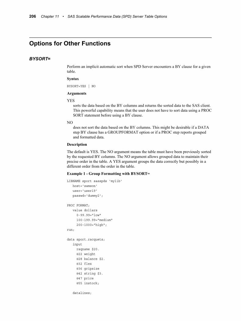
Options for Other Functions
BYSORT=Perform an implicit automatic sort when SPD Server encounters a BY clause for a given table.
Syntax
BYSORT=YES | NO
Arguments
YESsorts the data based on the BY columns and returns the sorted data to the SAS client. This powerful capability means that the user does not have to sort data using a PROC SORT statement before using a BY clause.
NOdoes not sort the data based on the BY columns. This might be desirable if a DATA step BY clause has a GROUPFORMAT option or if a PROC step reports grouped and formatted data.
Description
The default is YES. The NO argument means the table must have been previously sorted by the requested BY columns. The NO argument allows grouped data to maintain their precise order in the table. A YES argument groups the data correctly but possibly in a different order from the order in the table.
Example 1 - Group Formatting with BYSORT=
LIBNAME sport sasspds 'mylib' host='samson' user='user19' passwd='dummy2';
PROC FORMAT; value dollars 0-99.99="low" 100-199.99="medium" 200-1000="high";run;
data sport.racquets; input raqname $20. @22 weight @28 balance $2. @32 flex @36 gripsize @42 string $3. @47 price @55 instock;
datalines;
206 Chapter 11 • SAS Scalable Performance Data (SPD) Server Table Options

Solo Junior 10.1 N 2 3.75 syn 50.00 6Solo Lobber 11.3 N 10 5.5 syn 160.00 1Solo Queensize 10.9 HH 6 5.0 syn 130.00 3Solo Kingsize 13.1 HH 5 5.6 syn 140.00 3;
PROC PRINT data=sport.racquets (bysort=yes); var raqname instock; by price; format price dollars.;title 'Solo Brand Racquets by Price Level';run;
Output 11.1 Report Output with BYSORT=
Solo Brand Racquets by Price Level
---------------------------- Price=low ---------------------------
OBS RAQNAME INSTOCK
1 Solo Junior 6
-------------------------- Price=medium --------------------------
OBS RAQNAME INSTOCK
3 Solo Queensize 3
4 Solo Kingsize 3
2 Solo Lobber 1
Example 2 - Group Formatting without BYSORT=
PROC PRINT data=sport.racquets (bysort=no); var raqname instock; by price; format price dollars.;title 'Solo Brand Racquets by Price Level';run;
Options for Other Functions 207
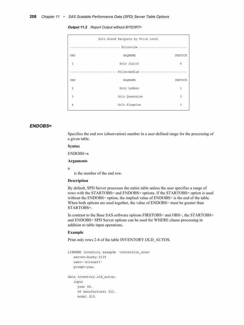
Output 11.2 Report Output without BYSORT=
Solo Brand Racquets by Price Level
---------------------------- Price=low ---------------------------
OBS RAQNAME INSTOCK
1 Solo Junior 6
-------------------------- Price=medium --------------------------
OBS RAQNAME INSTOCK
2 Solo Lobber 1
3 Solo Queensize 3
4 Solo Kingsize 3
ENDOBS=Specifies the end row (observation) number in a user-defined range for the processing of a given table.
Syntax
ENDOBS=n
Arguments
nis the number of the end row.
Description
By default, SPD Server processes the entire table unless the user specifies a range of rows with the STARTOBS= and ENDOBS= options. If the STARTOBS= option is used without the ENDOBS= option, the implied value of ENDOBS= is the end of the table. When both options are used together, the value of ENDOBS= must be greater than STARTOBS=.
In contrast to the Base SAS software options FIRSTOBS= and OBS=, the STARTOBS= and ENDOBS= SPD Server options can be used for WHERE clause processing in addition to table input operations.
Example
Print only rows 2-4 of the table INVENTORY.OLD_AUTOS.
LIBNAME inventory sasspds 'conversion_area' server=husky.5105 user='siteusr1' prompt=yes;
data inventory.old_autos; input year $4. @6 manufacturer $12. model $10.
208 Chapter 11 • SAS Scalable Performance Data (SPD) Server Table Options
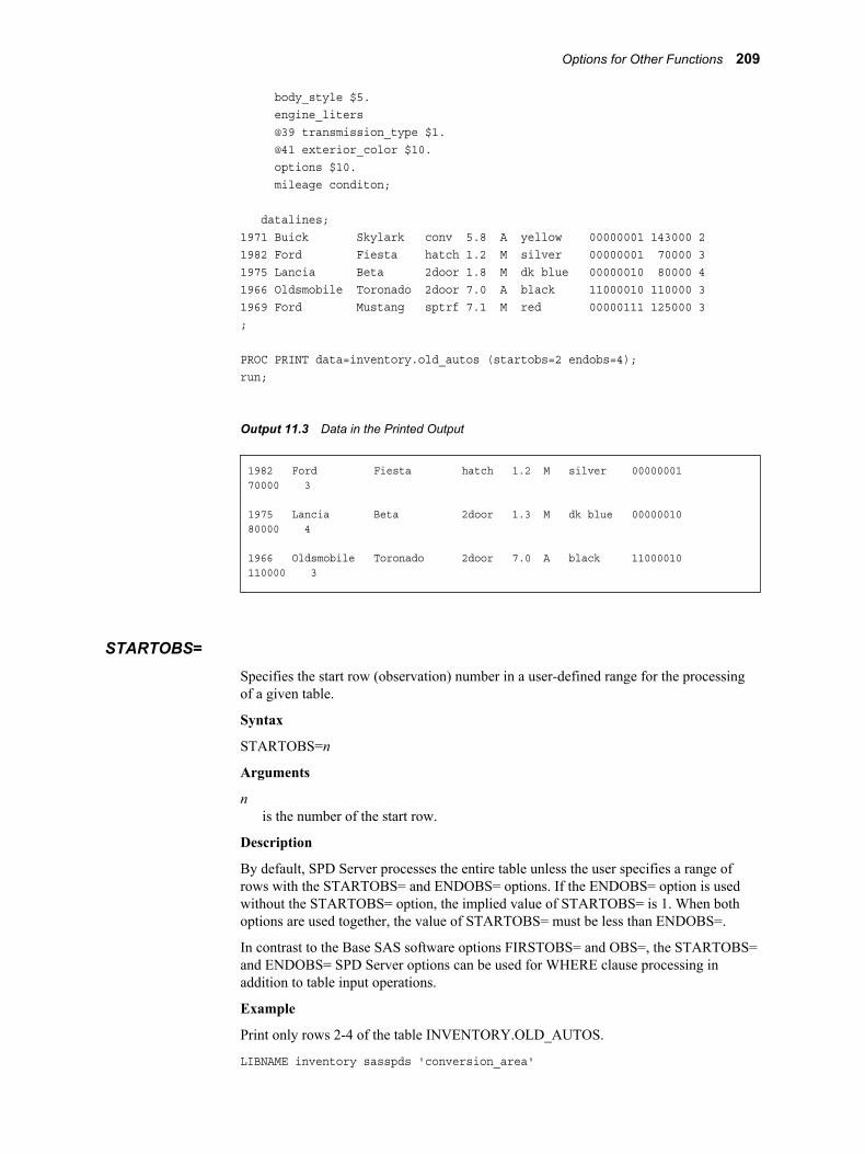
body_style $5. engine_liters @39 transmission_type $1. @41 exterior_color $10. options $10. mileage conditon;
datalines;1971 Buick Skylark conv 5.8 A yellow 00000001 143000 21982 Ford Fiesta hatch 1.2 M silver 00000001 70000 31975 Lancia Beta 2door 1.8 M dk blue 00000010 80000 41966 Oldsmobile Toronado 2door 7.0 A black 11000010 110000 31969 Ford Mustang sptrf 7.1 M red 00000111 125000 3;
PROC PRINT data=inventory.old_autos (startobs=2 endobs=4);run;
Output 11.3 Data in the Printed Output
1982 Ford Fiesta hatch 1.2 M silver 00000001 70000 3
1975 Lancia Beta 2door 1.3 M dk blue 00000010 80000 4
1966 Oldsmobile Toronado 2door 7.0 A black 11000010 110000 3
STARTOBS=Specifies the start row (observation) number in a user-defined range for the processing of a given table.
Syntax
STARTOBS=n
Arguments
nis the number of the start row.
Description
By default, SPD Server processes the entire table unless the user specifies a range of rows with the STARTOBS= and ENDOBS= options. If the ENDOBS= option is used without the STARTOBS= option, the implied value of STARTOBS= is 1. When both options are used together, the value of STARTOBS= must be less than ENDOBS=.
In contrast to the Base SAS software options FIRSTOBS= and OBS=, the STARTOBS= and ENDOBS= SPD Server options can be used for WHERE clause processing in addition to table input operations.
Example
Print only rows 2-4 of the table INVENTORY.OLD_AUTOS.
LIBNAME inventory sasspds 'conversion_area'
Options for Other Functions 209
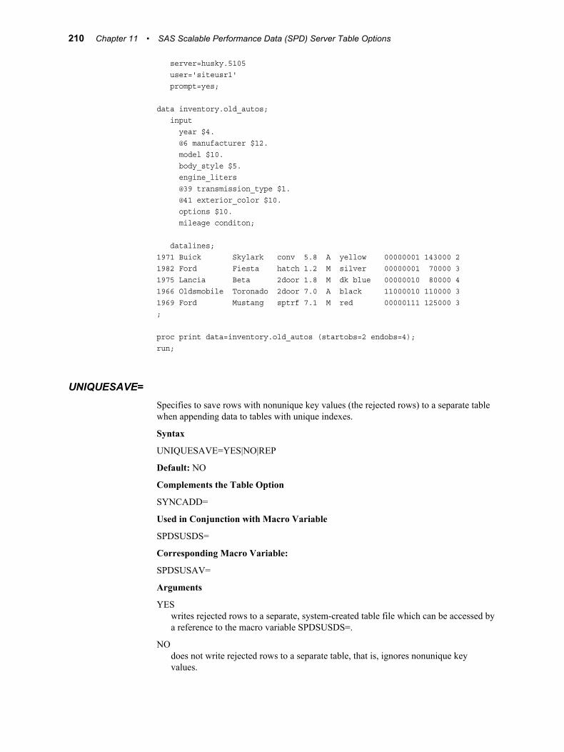
server=husky.5105 user='siteusr1' prompt=yes;
data inventory.old_autos; input year $4. @6 manufacturer $12. model $10. body_style $5. engine_liters @39 transmission_type $1. @41 exterior_color $10. options $10. mileage conditon;
datalines;1971 Buick Skylark conv 5.8 A yellow 00000001 143000 21982 Ford Fiesta hatch 1.2 M silver 00000001 70000 31975 Lancia Beta 2door 1.8 M dk blue 00000010 80000 41966 Oldsmobile Toronado 2door 7.0 A black 11000010 110000 31969 Ford Mustang sptrf 7.1 M red 00000111 125000 3;
proc print data=inventory.old_autos (startobs=2 endobs=4);run;
UNIQUESAVE=Specifies to save rows with nonunique key values (the rejected rows) to a separate table when appending data to tables with unique indexes.
Syntax
UNIQUESAVE=YES|NO|REP
Default: NO
Complements the Table Option
SYNCADD=
Used in Conjunction with Macro Variable
SPDSUSDS=
Corresponding Macro Variable:
SPDSUSAV=
Arguments
YESwrites rejected rows to a separate, system-created table file which can be accessed by a reference to the macro variable SPDSUSDS=.
NOdoes not write rejected rows to a separate table, that is, ignores nonunique key values.
210 Chapter 11 • SAS Scalable Performance Data (SPD) Server Table Options
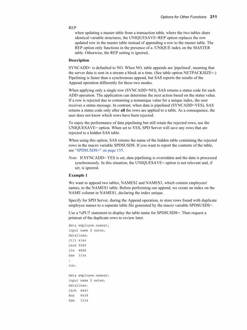
REPwhen updating a master table from a transaction table, where the two tables share identical variable structures, the UNIQUESAVE=REP option replaces the row updated row in the master table instead of appending a row to the master table. The REP option only functions in the presence of a /UNIQUE index on the MASTER table. Otherwise, the REP setting is ignored..
Description
SYNCADD= is defaulted to NO. When NO, table appends are 'pipelined', meaning that the server data is sent in a stream a block at a time. (See table option NETPACKSIZE=.) Pipelining is faster than a synchronous append, but SAS reports the results of the Append operation differently for these two modes.
When applying only a single row (SYNCADD=NO), SAS returns a status code for each ADD operation. The application can determine the next action based on the status value. If a row is rejected due to containing a nonunique value for a unique index, the user receives a status message. In contrast, when data is pipelined (SYNCADD=YES), SAS returns a status code only after all the rows are applied to a table. As a consequence, the user does not know which rows have been rejected.
To enjoy the performance of data pipelining but still retain the rejected rows, use the UNIQUESAVE= option. When set to YES, SPD Server will save any rows that are rejected to a hidden SAS table.
When using this option, SAS returns the name of the hidden table containing the rejected rows in the macro variable SPDSUSDS. If you want to report the contents of the table, see “SPDSUSDS=” on page 155.
Note: If SYNCADD= YES is set, data pipelining is overridden and the data is processed synchronously. In this situation, the UNIQUESAVE= option is not relevant and, if set, is ignored.
Example 1
We want to append two tables, NAMES2 and NAMES3, which contain employees' names, to the NAMES1 table. Before performing our append, we create an index on the NAME column in NAMES1, declaring the index unique.
Specify for SPD Server, during the Append operation, to store rows found with duplicate employee names to a separate table file generated by the macro variable SPDSUSDS=.
Use a %PUT statement to display the table name for SPDSUSDS=. Then request a printout of the duplicate rows to review later.
data employee.names1;input name $ exten;datalines;Jill 4344Jack 5589Jim 8888Sam 3334;run;
data employee.names2;input name $ exten;datalines;Jack 4443Ann 8438Sam 3334
Options for Other Functions 211
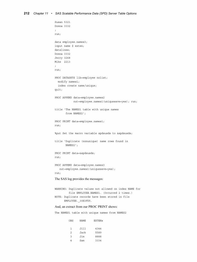
Susan 5321Donna 3332;run;
data employee.names3;input name $ exten;datalines;Donna 3332Jerry 3268Mike 2213;run;
PROC DATASETS lib=employee nolist; modify names1; index create name/unique;quit;
PROC APPEND data=employee.names2 out=employee.names1(uniquesave=yes); run;
title 'The NAMES1 table with unique names from NAMES2';
PROC PRINT data=employee.names1;run;
%put Set the macro variable spdsusds to &spdsusds;
title 'Duplicate (nonunique) name rows found in NAMES2';
PROC PRINT data=&spdsusds;run;
PROC APPEND data=employee.names3 out=employee.names1(uniquesave=yes);run;
The SAS log provides the messages:
WARNING: Duplicate values not allowed on index NAME for file EMPLOYEE.NAMES1. (Occurred 2 times.)NOTE: Duplicate records have been stored in file EMPLOYEE._30E3FD5.
And, an extract from our PROC PRINT shows:
The NAMES1 table with unique names from NAMES2
OBS NAME EXTENs
1 Jill 4344 2 Jack 5589 3 Jim 8888 4 Sam 3334
212 Chapter 11 • SAS Scalable Performance Data (SPD) Server Table Options

5 Ann 8438 6 Susan 5321 7 Donna 3332
Duplicate (nonunique) name rows found in NAMES2
OBS NAME EXTEN XXX00000
1 Jack 4443 NAME 2 Sam 3334 NAME
Example 2
Use the UNIQUESAVE=REP option to perform an update / append case using PROC APPEND instead of a DATA step:
* A MASTER table to update. ID *//* will get a UNIQUE index */
DATA SPDS.MASTER; INPUT ID VALUE $; CARDS; 1 one 2 two 3 three ;
PROC DATASETS LIB=SPDS; MODIFY MASTER; INDEX CREATE ID/UNIQUE; QUIT;
/* A transaction table TRANS to use to */ /* drive update/appends to MASTER */
DATA SPDS.TRANS; INPUT ID VALUE $; 1 ONE 3 THREE 4 FOUR 4 FOUR* ;
/* Use of UNIQUESAVE=REP to update/append */ /* TRANS rows to MASTER based on whether */ /* TRANS records have an ID column that */ /* matches an existing row from the MASTER */ /* table. Update MASTER rows with a match, */ /* otherwise append TRANS row to MASTER */
PROC APPEND DATA=SPDS.TRANS OUT=SPDS.MASTER(UNIQUESAVE=REP); run;
Output of the resulting MASTER table would look like:
Options for Other Functions 213

Obs ID VALUE
1 1 ONE 2 2 two 3 2 THREE 4 4 FOUR*
VERBOSE=Provides details of all indexes and ACL information associated with an SPD Server table.
Syntax
VERBOSE= YES | NO
Arguments
YESrequests detail information for the indexes, ACLs, and other SPD Server table values. This argument must be used with the CONTENTS procedure.
NOsuppresses detail information for the indexes, ACLs, and other SPD Server table values. This is the default.
Example
Request details of all the indexes for the table TEMP1 in the domain SPDS45.
PROC CONTENTS data=SPDS45 (verbose=yes);run;
214 Chapter 11 • SAS Scalable Performance Data (SPD) Server Table Options

Output 11.4 Output 14.4: Details of Table TEMP1 Indexes in Domain SPDS45
The CONTENTS Procedure
Data Set Name SPDS45.TEMP1 Observations 1000Member Type DATA Variables 2Engine SASSPDS Indexes 2Created Tuesday, May 10, 2005 10:00:02 AM Observation Length 16Last Modified Tuesday, May 10, 2005 11:01:36 AM Deleted Observations 0Protection Compressed NOData Set Type Sorted NOLabelData Representation DefaultEncoding Default
Engine / Host Dependent Information
Blocking Factor (obs/block) 2047 ACL Entry NO ACL User Access(R,W,A,C) (Y,Y,Y,Y) ACL User Name ANONYMOU ACL Owner Name ANONYMOU Data Set is Ranged NO Alphabetic List of Index Info . Bitmap index (No Global Index ) i Keyvalue (Min) 1 Keyvalue (Max) 100 # of Discrete values 100 Bitmap index (No Global Index ) j Keyvalue (Min) 1 Keyvalue (Max) 10 # of Discrete values 10 Data Partsize 16777216
Alphabetic List of Variables and Attributes
* Variable Type Len
1 i Num 8 2 j Num 9
Alphabetic List of Indexes and Attributes
# of Unique * Index Values
1 i 100 2 j 10
Options for Other Functions 215
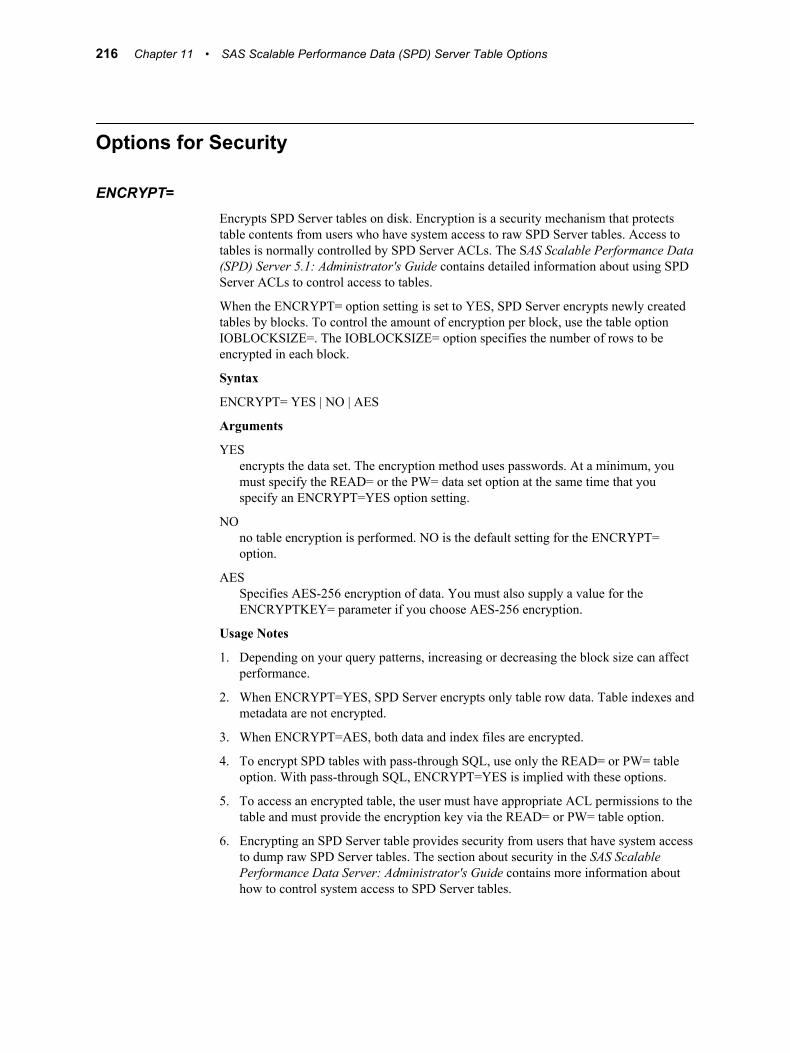
Options for Security
ENCRYPT=Encrypts SPD Server tables on disk. Encryption is a security mechanism that protects table contents from users who have system access to raw SPD Server tables. Access to tables is normally controlled by SPD Server ACLs. The SAS Scalable Performance Data (SPD) Server 5.1: Administrator's Guide contains detailed information about using SPD Server ACLs to control access to tables.
When the ENCRYPT= option setting is set to YES, SPD Server encrypts newly created tables by blocks. To control the amount of encryption per block, use the table option IOBLOCKSIZE=. The IOBLOCKSIZE= option specifies the number of rows to be encrypted in each block.
Syntax
ENCRYPT= YES | NO | AES
Arguments
YESencrypts the data set. The encryption method uses passwords. At a minimum, you must specify the READ= or the PW= data set option at the same time that you specify an ENCRYPT=YES option setting.
NOno table encryption is performed. NO is the default setting for the ENCRYPT= option.
AESSpecifies AES-256 encryption of data. You must also supply a value for the ENCRYPTKEY= parameter if you choose AES-256 encryption.
Usage Notes
1. Depending on your query patterns, increasing or decreasing the block size can affect performance.
2. When ENCRYPT=YES, SPD Server encrypts only table row data. Table indexes and metadata are not encrypted.
3. When ENCRYPT=AES, both data and index files are encrypted.
4. To encrypt SPD tables with pass-through SQL, use only the READ= or PW= table option. With pass-through SQL, ENCRYPT=YES is implied with these options.
5. To access an encrypted table, the user must have appropriate ACL permissions to the table and must provide the encryption key via the READ= or PW= table option.
6. Encrypting an SPD Server table provides security from users that have system access to dump raw SPD Server tables. The section about security in the SAS Scalable Performance Data Server: Administrator's Guide contains more information about how to control system access to SPD Server tables.
216 Chapter 11 • SAS Scalable Performance Data (SPD) Server Table Options

ENCRYPTKEY=When you use the ENCRYPT=AES option setting to specify AES-256 encryption, you must use the ENCRYPTKEY= option setting to specify a text string value that will enable the RSA 256-bit encryption key to encode data and indexes at rest on the server disk.
Options for Security 217

218 Chapter 11 • SAS Scalable Performance Data (SPD) Server Table Options
Chapter 12
SAS Scalable Performance Data (SPD) Server Formats and Informats
Introduction . . . . . . . . . . . . . . . . . . . . . . . . . . . . . . . . . . . . . . . . . . . . . . . . . . . . . . . . . 219
Formats . . . . . . . . . . . . . . . . . . . . . . . . . . . . . . . . . . . . . . . . . . . . . . . . . . . . . . . . . . . . 219List of Formats . . . . . . . . . . . . . . . . . . . . . . . . . . . . . . . . . . . . . . . . . . . . . . . . . . . . 219Formats Example . . . . . . . . . . . . . . . . . . . . . . . . . . . . . . . . . . . . . . . . . . . . . . . . . . 221
User-Defined Formats . . . . . . . . . . . . . . . . . . . . . . . . . . . . . . . . . . . . . . . . . . . . . . . . 221
Informats . . . . . . . . . . . . . . . . . . . . . . . . . . . . . . . . . . . . . . . . . . . . . . . . . . . . . . . . . . . 225
IntroductionSAS Scalable Performance Data (SPD) Server supports some of the more commonly used SAS format and informats. Use these in your SQL pass-through code when you want SAS Scalable Performance Data (SPD) Server to associate a data set variable with a specific format.
A general reminder about formats: A format is applied to data set variables as it is written out. Informats are applied as the data set variable is being read.
Formats
List of Formats• $ — Writes standard character data
• $BINARY — Converts character values to binary representation
• $CHAR — Writes standard character data
• $HEX — Converts character values to hexadecimal representation
• $OCTAL — Converts character values to octal representation
• $QUOTE — Converts character values to quoted strings
• $VARYING — Writes varying length values
• BEST — SAS Scalable Performance Data (SPD) Server system chooses best notation
219

• BINARY — Converts numeric values to binary representation
• COMMA — Writes numeric values with commas and decimal points
• COMMAX — Writes numeric values with commas and decimal points (European style)
• DATE — Writes date values (ddmmmyy)
• DATETIME — Writes date time values (ddmmmyy:hh:mm:ss.ss)
• DAY — Writes day of month
• DDMMYY — Writes date values (ddmmyy)
• DOLLAR — Writes numeric values with dollar signs, commas, and decimal points
• DOLLARX — Writes numeric values with dollar signs, commas, and decimal points (European style)
• DOWNAME — Writes name of day of the week
• E — Writes scientific notation
• F — Writes scientific notation
• FRACT — Converts values to fractions
• HEX -- Converts real binary (floating-point) numbers to hexadecimal representation
• HHMM — Writes hours and minutes
• HOUR — Writes hours and decimal fractions of hours
• IB — Writes integer binary values
• MMDDYY — Writes date values (mmddyy)
• MMSS — Writes minutes and seconds
• MMYY — Writes month and year, separated by a 'M'
• MONNAME — Writes name of month
• MONTH — Writes month of year
• MONYY — Writes month and year
• NEGPAREN — Displays negative values in parentheses
• OCTAL — Converts numeric values to octal representation
• PD — Writes packed decimal data
• PERCENT — Prints numbers as percentages
• PIB — Writes positive integer binary values
• QTR — Writes quarter of year
• RB — Writes real binary (floating-point) data
• SSN — Writes Social Security numbers
• TIME — Writes hours, minutes, and seconds
• TOD — Writes the time portion of datetime values
• w.d — Writes standard numeric data
• WEEKDATE — Writes day of week and date (day-of-week, month-name dd, yy)
• WEEKDATX — Writes day of week and date (day-of-week, dd month-name yy)
220 Chapter 12 • SAS Scalable Performance Data (SPD) Server Formats and Informats

• WEEKDAY — Writes day of week
• WORDDATE — Writes date with name of month, day, and year (month-name dd, yyyy)
• WORDDATX — Writes date with day, name of month, and year (dd month-name yyyy)
• WORDF — Converts numeric values to words
• WORDS — Converts numeric values to words (fractions as words)
• YEAR — Writes year part of date value
• YYMM — Write year and month, separated by a 'M'
• YYMMDD — Writes day values (yymmdd)
• YYMON — Writes year and month abbreviation
• YYQ — Writes year and quarter, separated by a 'Q'
• Z — Writes leading 0s
• ZD — Writes data in zoned decimal format
Note: Formats which begin with a '$' sign are character formats. Otherwise, the format accepts numeric values.
Formats ExampleUse the dollar. format to convert numeric sales figures into dollar values. Suppose you have an SPD Server data set Sales with a single numeric variable salesite representing the total sales for a given site. Using SQL pass-through, create a new data set containing the sales in dollar format.
PROC SQL;connect to sasspds (dbq='tmp' user='anonymous' host='localhost' serv='5127');
execute(create table money as select salesite format=dollar. from sales)
by sasspds;
quit;
User-Defined FormatsTo create and access user-defined formats in SPD Server, you must do the following::
User-Defined Formats 221

• The user-defined formats must be created on the architecture where they will be used. For example, if the format is to be used on a Windows server, the format must be created on a Windows machine.
• The user-defined formats must be created in a domain called formats.
• You must make an SPD Server LIBNAME assignment to the domain called formats.
• You must specify
options fmtsearch=(formats);
so that SAS can also find the formats to verify them.
SPD Server does not require that your data and your user-defined formats reside in the same domain. SPD Server will always look in the domain that is named formats when the operating system encounters any call for user-defined formats.
The following example code shows how user-defined formats can be referenced:
• in parallel GROUP BY statements
• in a WHERE clause within a PROC PRINT step, and
• in a WHERE clause referenced in explicit SQL.
The example includes the creation of the user-defined formats and a test table. The example also provides changes to configuration files (spdsserv.parm and libnames.parm) that normally would be made by your SPD Server administrator. For more information about configuring spdsserv.parm files, see Chapter 11, “Setting Up SAS Scalable Performance Data (SPD) Server Parameter Files ,” in SAS Scalable Performance Data Server: Administrator's Guide. For more information about configuring libname.parm files, see Chapter 12, “Setting Up SAS Scalable Performance Data (SPD) Server Libname Parameter Files ,” in SAS Scalable Performance Data Server: Administrator's Guide
The example uses the following SPD Server spdsserv.parm file:
SORTSIZE=8M;INDEX_SORTSIZE=8M;BINBUFSIZE=32K;INDEX_MAXMEMORY=8M;NOCOREFILE;SEQIOBUFMIN=64K;RANIOBUFMIN=4K;NOALLOWMMAP;MAXWHTHREADS=16;WHERECOSTING;RANDOMPLACEDPF;FMTDOMAIN=FORMATS;FMTNAMENODE=d8488 ;FMTNAMEPORT=5200;
The example uses the following SPD Server libnames.parm file:
LIBNAME=tmp pathname=c:\temp;LIBNAME=formats pathname=c:\data\formats;
Here is the complete example code with comments::
222 Chapter 12 • SAS Scalable Performance Data (SPD) Server Formats and Informats
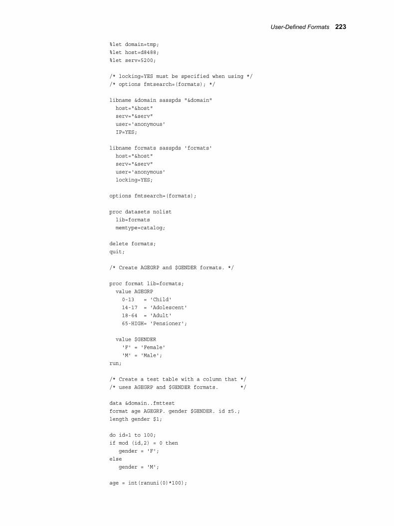
%let domain=tmp; %let host=d8488; %let serv=5200;
/* locking=YES must be specified when using */ /* options fmtsearch=(formats); */
libname &domain sasspds "&domain" host="&host" serv="&serv" user='anonymous' IP=YES;
libname formats sasspds 'formats' host="&host" serv="&serv" user='anonymous' locking=YES; options fmtsearch=(formats);
proc datasets nolist lib=formats memtype=catalog;
delete formats; quit;
/* Create AGEGRP and $GENDER formats. */
proc format lib=formats; value AGEGRP 0-13 = 'Child' 14-17 = 'Adolescent' 18-64 = 'Adult' 65-HIGH= 'Pensioner';
value $GENDER 'F' = 'Female' 'M' = 'Male';run;
/* Create a test table with a column that *//* uses AGEGRP and $GENDER formats. */
data &domain..fmttestformat age AGEGRP. gender $GENDER. id z5.;length gender $1;
do id=1 to 100;if mod (id,2) = 0 then gender = 'F';else gender = 'M';
age = int(ranuni(0)*100);
User-Defined Formats 223
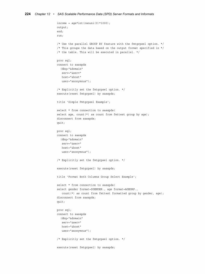
income = age*int(ranuni(0)*1000);output;end;run;
/* Use the parallel GROUP BY feature with the fmtgrpsel option. *//* This groups the data based on the output format specified in *//* the table. This will be executed in parallel. */
proc sql;connect to sasspds (dbq="&domain" serv="&serv" host="&host" user="anonymous");
/* Explicitly set the fmtgrpsel option. */execute(reset fmtgrpsel) by sasspds;
title 'Simple Fmtgrpsel Example';
select * from connection to sasspds(select age, count(*) as count from fmttest group by age);disconnect from sasspds;quit;
proc sql;connect to sasspds (dbq="&domain" serv="&serv" host="&host" user="anonymous");
/* Explicitly set the fmtgrpsel option. */
execute(reset fmtgrpsel) by sasspds;
title 'Format Both Columns Group Select Example';
select * from connection to sasspds(select gender format=$GENDER., age format=AGEGRP., count(*) as count from fmttest formatted group by gender, age);disconnect from sasspds;quit;
proc sql;connect to sasspds (dbq="&domain" serv="&serv" host="&host" user="anonymous");
/* Explicitly set the fmtgrpsel option. */
execute(reset fmtgrpsel) by sasspds;
224 Chapter 12 • SAS Scalable Performance Data (SPD) Server Formats and Informats

title1 'To use Format on Only One Column With Group Select';title2 'Override Column Format With a Standard Format';
select * from connection to sasspds (select gender format=$1., age format=AGEGRP., count(*) as count from fmttest formatted group by gender, age);
disconnect from sasspds;quit;
/* A WHERE clause that uses a format to subset */ /* data is pushed to the server. If it is not */ /* pushed to the server, the following warning */ /* message will be written to the SAS log: */ /* WARNING: Server is unable to execute the where clause. */
data temp; set &domain..fmttest where put (age, AGEGRP.) = 'Child'; run;
title 'Format in WHERE clause example';proc print data=temp; run;
/* This explicit SQL executes a WHERE clause that *//* references a user-defined format. */
title 'Explicit SQL with a User-Defined Format in a WHERE Clause';
proc sql;connect to sasspds (dbq="&domain" serv="&serv" host="&host" user="anonymous");
select * from connection to sasspds (select * from fmttest where put(age, AGEGRP.) eq 'Child');quit;
Informats• $ — Reads standard character data
• $BINARY — Converts binary values to character values
• $CB — Reads standard character data from column-binary files
• $CHAR — Reads character data with blanks
• $HEX — Converts hexadecimal data to character data
Informats 225
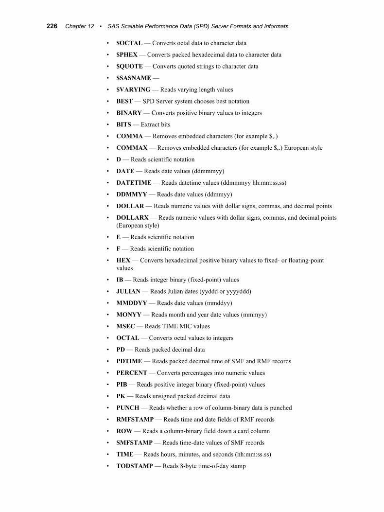
• $OCTAL — Converts octal data to character data
• $PHEX — Converts packed hexadecimal data to character data
• $QUOTE — Converts quoted strings to character data
• $SASNAME —
• $VARYING — Reads varying length values
• BEST — SPD Server system chooses best notation
• BINARY — Converts positive binary values to integers
• BITS — Extract bits
• COMMA — Removes embedded characters (for example $,.)
• COMMAX — Removes embedded characters (for example $,.) European style
• D — Reads scientific notation
• DATE — Reads date values (ddmmmyy)
• DATETIME — Reads datetime values (ddmmmyy hh:mm:ss.ss)
• DDMMYY — Reads date values (ddmmyy)
• DOLLAR — Reads numeric values with dollar signs, commas, and decimal points
• DOLLARX — Reads numeric values with dollar signs, commas, and decimal points (European style)
• E — Reads scientific notation
• F — Reads scientific notation
• HEX — Converts hexadecimal positive binary values to fixed- or floating-point values
• IB — Reads integer binary (fixed-point) values
• JULIAN — Reads Julian dates (yyddd or yyyyddd)
• MMDDYY — Reads date values (mmddyy)
• MONYY — Reads month and year date values (mmmyy)
• MSEC — Reads TIME MIC values
• OCTAL — Converts octal values to integers
• PD — Reads packed decimal data
• PDTIME — Reads packed decimal time of SMF and RMF records
• PERCENT — Converts percentages into numeric values
• PIB — Reads positive integer binary (fixed-point) values
• PK — Reads unsigned packed decimal data
• PUNCH — Reads whether a row of column-binary data is punched
• RMFSTAMP — Reads time and date fields of RMF records
• ROW — Reads a column-binary field down a card column
• SMFSTAMP — Reads time-date values of SMF records
• TIME — Reads hours, minutes, and seconds (hh:mm:ss.ss)
• TODSTAMP — Reads 8-byte time-of-day stamp
226 Chapter 12 • SAS Scalable Performance Data (SPD) Server Formats and Informats

• TU — Reads timer units
• YYMMDD — Reads date values (yymmdd)
• YYQ — Reads quarters of the year
Note: Informats that begin with a $ sign are character informats. Otherwise, the informat accepts numeric values.
The SQL procedure itself does not use the INFORMAT= modifier: it stores informats in its table definitions so that other procedures and the DATA step can use the information. SPD Server informats are provided now to allow for forward compatibility with future development.
Informats 227

228 Chapter 12 • SAS Scalable Performance Data (SPD) Server Formats and Informats
Chapter 13
SAS Scalable Performance Data (SPD) Server NLS Support
Overview of NLS . . . . . . . . . . . . . . . . . . . . . . . . . . . . . . . . . . . . . . . . . . . . . . . . . . . . . 229
Character Encoding . . . . . . . . . . . . . . . . . . . . . . . . . . . . . . . . . . . . . . . . . . . . . . . . . . 230Overview of Character Encoding . . . . . . . . . . . . . . . . . . . . . . . . . . . . . . . . . . . . . . 230What is Character Encoding? . . . . . . . . . . . . . . . . . . . . . . . . . . . . . . . . . . . . . . . . . 230Common Encodings . . . . . . . . . . . . . . . . . . . . . . . . . . . . . . . . . . . . . . . . . . . . . . . . 232
Moving Data across Environments with Different Encodings . . . . . . . . . . . . . . . . 233Transcoding . . . . . . . . . . . . . . . . . . . . . . . . . . . . . . . . . . . . . . . . . . . . . . . . . . . . . . 233How Base SAS Transcodes Data . . . . . . . . . . . . . . . . . . . . . . . . . . . . . . . . . . . . . . 234
Base SAS Encoding Behavior . . . . . . . . . . . . . . . . . . . . . . . . . . . . . . . . . . . . . . . . . . 234Overview of Base SAS Encoding . . . . . . . . . . . . . . . . . . . . . . . . . . . . . . . . . . . . . . 234SAS 9 Output Processing . . . . . . . . . . . . . . . . . . . . . . . . . . . . . . . . . . . . . . . . . . . . 235SAS 9 Input Processing . . . . . . . . . . . . . . . . . . . . . . . . . . . . . . . . . . . . . . . . . . . . . 235Reading and Writing External Files . . . . . . . . . . . . . . . . . . . . . . . . . . . . . . . . . . . . 235
Setting the Encoding for Base SAS Sessions . . . . . . . . . . . . . . . . . . . . . . . . . . . . . . 235
Changing the Encoding for Base SAS Sessions . . . . . . . . . . . . . . . . . . . . . . . . . . . . 236
NLS Support in SPD Server . . . . . . . . . . . . . . . . . . . . . . . . . . . . . . . . . . . . . . . . . . . 237Overview of NLS Support . . . . . . . . . . . . . . . . . . . . . . . . . . . . . . . . . . . . . . . . . . . 237SPD Server NLS Limitations . . . . . . . . . . . . . . . . . . . . . . . . . . . . . . . . . . . . . . . . . 237LIBNAME Option Restrictions: . . . . . . . . . . . . . . . . . . . . . . . . . . . . . . . . . . . . . . . 238
Overview of NLSNLS, or National Language Support, deals both with Internationalization and Localization of SAS software. Internationalization is the process of designing an application so that it can be adapted to different languages and regions, without requiring engineering changes. Often the term internationalization is abbreviated as i18n, because there are 18 letters between the first i and the last n. Localization is the process of adapting software for a particular region or language by adding locale-specific components and translating text. The term localization is often abbreviated as L10n, because there are 10 letters between the L and the n. Translation of user interface, messages, and documentation is a large part (but not all) of localization. Localizers also verify that the formatting of dates, numbers, currencies, and so on, conforms to local requirements.
SAS 9 contains built-in support for NLS character set encoding and locale choices. Users access the NLS encoding and locale choices through various SAS, LIBNAME,
229

and data set options. SAS Scalable Performance Data (SPD) Server and SAS together offer basic levels of NLS support. This document describes the basic entities of NLS support and how they are implemented in SPD Server
Character Encoding
Overview of Character EncodingAll input to a computer is represented internally as numbers. The computer assigns a number to each character – technically, the number is a binary number (base 2 numbering system, consisting of 0s and 1s).
Because most of us do not think in binary numbers, computers provide hexadecimal (base 16 numbering system) representation as a shorthand for binary representation. For example, for the decimal number 167, it is easier to understand the hexadecimal number A7 than the equivalent binary number 10100111. Therefore, you can think of the computer's internal numeric representation of all data as a hexadecimal number.
What is Character Encoding?All data that is stored, transmitted, or processed by a computer is in an encoding. An encoding maps each character to a unique numeric representation. For example:
1. You press a key on a keyboard, like the uppercase letter A.
2. The computer assigns the internal numeric representation, that is, a unique hexadecimal number.
3. To display or print the character, the computer uses the font (graphical representation) that matches the numeric representation, that is, the uppercase letter A.
To assign the numeric representation to a character, an encoding uses a code page, which is an ordered set of characters in which a numeric index (code point value) is associated with each character. The position of a character on the code page determines its two-digit hexadecimal number. The first digit of the hexadecimal number is determined by the column, and the second digit by the row. For example, the following is the code page for the Windows Latin1 encoding. The numeric representation for the uppercase A is the hexadecimal number 41, and the numeric representation for the equal sign (=) is the hexadecimal number 3D.
230 Chapter 13 • SAS Scalable Performance Data (SPD) Server NLS Support
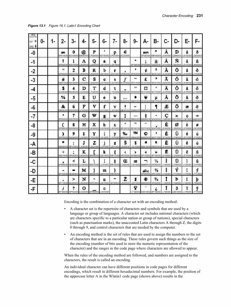
Figure 13.1 Figure 16.1: Latin1 Encoding Chart
Encoding is the combination of a character set with an encoding method:
• A character set is the repertoire of characters and symbols that are used by a language or group of languages. A character set includes national characters (which are characters specific to a particular nation or group of nations), special characters (such as punctuation marks), the unaccented Latin characters A through Z, the digits 0 through 9, and control characters that are needed by the computer.
• An encoding method is the set of rules that are used to assign the numbers to the set of characters that are in an encoding. These rules govern such things as the size of the encoding (number of bits used to store the numeric representation of the character) and the ranges in the code page where characters are allowed to appear.
When the rules of the encoding method are followed, and numbers are assigned to the characters, the result is called an encoding.
An individual character can have different positions in code pages for different encodings, which result in different hexadecimal numbers. For example, the position of the uppercase letter A in the Wlatin1 code page (shown above) results in the
Character Encoding 231

hexadecimal number 41, while in the following Danish EBCDIC code page, the position of the uppercase letter A results in the hexadecimal number C1.
Figure 13.2 Figure 16.2: Danish EBCDIC Code Page
Common EncodingsThere are many encodings that address the requirements of different languages. Very few languages use only the 26 characters A through Z of the Latin alphabet. In addition, there are different encodings to address different operating system standards.
An encoding that represents each character in one byte is a single-byte character set (SBCS). A single-byte character set can be either 7 bits (providing up to 128 characters) or 8 bits (providing up to 256 characters). An example of an 8-bit SBCS is the Latin1 encoding (represents the characters of Western Europe). (Note that the term octet, for the international community, is an 8-bit byte. Because a byte is not 8 bits in all computer systems, octet provides an unambiguous term.)
A multiple-byte character set (MBCS) is a mixed-width encoding in which some characters consist of more than one byte. For example, the Japanese, Korean, Simplified
232 Chapter 13 • SAS Scalable Performance Data (SPD) Server NLS Support

Chinese, and Traditional Chinese are MBCS encodings. A double-byte character set (DBCS) is a specific type of an MBCS encoding that includes characters that consist of two bytes.
The following are common encodings:
ASCII (American Standard Code for Information Interchange)Is a 7-bit encoding for the United States that provides 128 character combinations. The encoding contains characters for uppercase and lowercase English, American English punctuation, base 10 numbers, and a few control characters. The set of 128 characters is the one common denominator that is contained in most encodings, excluding EBCDIC-based encodings. ASCII is used by personal computers.
ISO (International Organization for Standardization) 646 familyIs a 7-bit encoding that is an international standard and provides 128 character combinations. The ISO 646 family of encodings is like ASCII except for 12 code points for national variants. The 12 national variants represent specific characters needed for a particular language.
EBCDIC (Extended Binary Coded Decimal Interchange Code) familyIs an 8-bit encoding that provides 256 character combinations. There are multiple EBCDIC-based encodings. EBCDIC is used on IBM mainframes and most IBM midrange computers. EBCDIC follows ISO 646 conventions to facilitate translations between itself and 7-bit ASCII-based encodings. Characters A through Z and 0 through 9 are mapped to the same code points on all EBCDIC code pages. The rest of the code points can be used for special characters and national characters, depending on the encoding.
ISO 8859 family and Windows familyIs an 8-bit extension of ASCII that supports all of the ASCII code points and adds 12 more, providing 256 character combinations. Latin1, which is officially named ISO-8859-1, is the most frequently used member of the ISO 8859 family of encodings. In addition to the ASCII characters, Latin1 contains accented characters, other letters needed for languages of Western Europe, and some special characters.
UnicodeUses two bytes for each character rather than one and provides up to 65,536 character combinations. Unicode can handle the scripts of basically all of the world's languages. For example, the Japanese language, which has thousands of characters, uses a 16-bit, multiple-byte character set. There are various forms of Unicode, including UTF-8, UTF-16, and UTF-32.
Moving Data across Environments with Different Encodings
TranscodingAlthough it is easy to move data across environments that use the same encoding, it can be more difficult to move data across environments that use different encodings. When the encoding of a file is incompatible with the computer environment's encoding, transcoding occurs.
Transcoding is the process of mapping data from one encoding to another, such as mapping data from an ASCII-based encoding to an EBCDIC-based encoding.
Moving Data across Environments with Different Encodings 233
Transcoding is not translating from one language to another; transcoding is remapping of characters.
For example, consider a file that was created on a UNIX platform that uses the Latin1 encoding, then moved to an IBM mainframe that uses the Danish EBCDIC encoding. When the file is processed on the IBM mainframe, the data is remapped from the Latin1 encoding to the Danish EBCDIC encoding. If the data contains a dollar sign ($), the hexadecimal number is converted from 24 to 67.
Transcoding can occur in the following situations:
• when you move a SAS file from one platform to another and the file's encoding is incompatible with the current session encoding. An example might be moving a SAS file from a z/OS operating environment with an EBCDIC-based encoding to a Windows operating environment with an ASCII-based encoding.
• when you share data between two SAS sessions (like in a client/server environment) that have incompatible session encodings.
• when you read and write an external file.
How Base SAS Transcodes DataBase SAS provides transcoding when you move data and applications from one environment to another. To transcode one encoding to another, SAS uses translation tables, like the one that maps Wlatin2 (Windows) to ISO Latin2 (UNIX).
For example, when you
• use the CPORT and CIMPORT procedures to create a transport file, SAS automatically uses translation tables to transcode one encoding to another and back again. First, the data is converted from the source encoding to transport format, then the data is converted from the transport format to the target encoding.
• process a SAS data set that has an encoding that is different from the current session encoding, SAS automatically uses CEDA (cross environment data access) software to transcode data. (CEDA is the same software in SAS that converts a SAS file to the correct data representation when you move a file from one platform to another.)
Base SAS Encoding Behavior
Overview of Base SAS EncodingFor Base SAS files (not SPD Server), the encoding support depends on the version of SAS that created the file:
• Data sets created in SAS 9 automatically have an encoding attribute, which is stamped in the descriptor portion of the file.
• Data sets created in SAS 8 do not have an encoding value stamped on the file; they are assumed to be in the session encoding of the host environment.
The NLS features in SPD Server only support encoding from SAS 9.
234 Chapter 13 • SAS Scalable Performance Data (SPD) Server NLS Support
SAS 9 Output ProcessingFor SAS 9 data sets (not SPD Server), encoding is determined as follows:
• For a new output file, the data is written to the file using the current session encoding.
• For a new output file that is created with the OUTREP= option, which specifies a data representation different from the current session, the data is written to the file using the default session encoding for the operating system that is based on the specified OUTREP= value.
• For output processing that replaces an existing file, the new file inherits the encoding of the existing file.
• For output processing that replaces an existing file that is from another platform or if the existing file has no encoding stamped on it, the current session encoding is used.
SAS 9 Input ProcessingFor input (read) processing in SAS 9 (not SPD Server), encoding behavior is as follows:
• If the session encoding and the encoding that is stamped on the file are incompatible, the data is transcoded to the session encoding. For example, if the current session encoding is ASCII and the encoding that is stamped on the file is EBCDIC, SAS transcodes the data from EBCDIC to ASCII.
• If a file does not have an encoding stamped on it, SAS transcodes the data only if the file's data representation is different from the current session.
Reading and Writing External FilesSAS reads and writes external files using the current session encoding. SAS assumes that the external file is in the same encoding as the session encoding. For example, if you are creating a new SAS data set by reading an external file, SAS assumes that the file's encoding is the same as the session encoding. If it is not, the data could be written to the new SAS data set incorrectly.
Setting the Encoding for Base SAS SessionsWhen SAS 9 is installed, the Base SAS (not SPD Server) default encoding is host dependent and is determined by the default settings for several SAS system options. Here are three system options that you should be familiar with:
ENCODING=establishes the session encoding, which is the encoding that SAS uses to process syntax, process SAS data sets, and read and write external files. The default value is host dependent; all are SBCS encodings:
Setting the Encoding for Base SAS Sessions 235

Table 13.1 Default Session Encodings
Host Value Description
OpenVMS Latin1 Western (ISO)
z/OS OPEN_ED_1047 OpenEdition EBCDIC cp1047-Latin1
UNIX Latin1 Western (ISO)
Windows WLatin1 Western (Windows)
LOCALE=specifies the locale of the SAS session. The locale reflects the local language, conventions, and culture for a particular geographical region. A locale's conventions can include the formatting of dates, times, and numbers, and printer preferences like paper size. Specifying a locale also automatically sets the default encoding that establishes the session encoding; a locale has a common encoding that is used most often for a particular operating environment. The default locale is English, and the common encodings for English are the defaults above for ENCODING=.
NONLSCOMPATMODE | NLSCOMPATMODEprovides national language compatibility for non-English data processing using native characters. For SAS 9, the default is NONLSCOMPATMODE, which provides consistency for running SAS on multiple systems. NONLSCOMPATMODE specifies that data is to be processed in the encoding that is set by the ENCODING= or LOCALE= system option.
Changing the Encoding for Base SAS SessionsYou can change the session encoding by using the LOCALE= system option, the ENCODING= system option, or both. Note that valid values for both options are host dependent.
Here is how you can set the Base SAS (not SPD Server) session encoding when NONLSCOMPATMODE is specified:
• You can specify the LOCALE= system option in a configuration file, at SAS invocation, in an OPTIONS statement, or in the SAS System Options window. In SAS 9, several NLS-related system options are automatically set, based on the value of LOCALE=. Most customers will implicitly set encoding with the LOCALE= system option.
• You can specify the ENCODING= system option in a configuration file or at SAS invocation.
• Here is how LOCALE= and ENCODING= interact:
• If a value is not specified for ENCODING= (that is, the installation default is set), then specifying a value for LOCALE= sets the encoding based on the LOCALE= value. In addition, values for the following system options are set based on the LOCALE= value: DFLANG=, TRANTAB=, DATESTYLE=, and PAPERSIZE=.
236 Chapter 13 • SAS Scalable Performance Data (SPD) Server NLS Support

• If a value is specified for ENCODING=, that value sets the session encoding and overrides LOCALE=.
• If the value specified for LOCALE= is not compatible with the value specified for ENCODING=, then the value for LOCALE= is used. A warning message is provided if ENCODING= and LOCALE= conflict.
• If the DBCS system option is set, which specifies that SAS process DBCS encodings, the values for DBCSLANG= and DBCSTYPE= system options determine the session encoding and the locale. These options are used for Asian languages or for English with DBCS extensions.
Here is an example of implicitly setting the Base SAS (not SPD Server) session encoding based on the specified locale when you invoke SAS:
sas9 -explorer -locale spanish
Here is an example of explicitly setting the Base SAS (not SPD Server) session encoding with the OPTIONS statement:
options encoding=wlatin2;
T I P Changing encoding for a SAS session does not affect SAS keywords, which remain in English, or SAS log output, which also remains in English.
NLS Support in SPD Server
Overview of NLS SupportSPD Server contains support for a subset of the SAS 9 NLS functions documented above. SPD Server uses encoding and locale currently only on SAS software.
Case-folding is defined as a process applied to a sequence of characters, in which those identified as non-uppercase are replaced by their uppercase equivalents. Linguistic collation is performing linguistic sorts based on linguistic sort keys. However, those functions have yet to be implemented in SPD Server production code.
All tables that are produced by SPD Server and SAS inherit the SAS session's default encoding and locale settings. By default, SPD Server code expects new tables to follow the current SAS session's encoding and locale. Table updates that append rows or update existing rows will perform transcoding to ensure that appended and updated table rows match the existing table encoding.
Wire transfer is in the character set encoding of the SAS session for transfers to and from the SPD Server host, unless SPD Server transcoding has been disabled. SPD Server transcoding is enabled or disabled by inserting a [NO]NLSTRANSCODE statement in the SPD Server spdsserv.parm parameter file.
SPD Server NLS Limitations
Affected DataSPD Server hosts are restricted in how they handle NLS character strings. SPD Server hosts are restricted to data that is contained in character columns in data sets and some metadata structures. The NLS support for SPD Server is functional for only table labels and variable labels.
NLS Support in SPD Server 237
Column names, index names, table names, and catalog names are not supported in the SPD Server NLS support. Column names, index names, table names, and catalog names are still dependent on ASCII support. SPD Server SQL is subject to the NLS same restrictions.
Pass-Through SQLSPD Server pass-through SQL does not support any NLS functions. Pass-through SQL operates in the encoding and locale of the SAS session that initiates the CONNECT to SASSPDS.
Case Folding and Sort SequencesSPD Server NLS code supports very limited English Latin1 and Polish Latin2 case folding for SBCS encodings. UTF8 case folding is limited to the ASCII range of UTF8 encoding. NLS Sort sequences for SPD Server 5.1 are restricted to lexical sorts for all combinations. Linguistic sorting is a subject for future SPD Server releases.
Indexes and OrderingIndexes in SPD Server are created in the table's encoding, and only support lexical ordering. If the client's encoding and locale settings match the SPD Server host table's encoding and locale settings, index use is unrestricted. Otherwise, index usage is restricted to certain predicates in WHERE clauses that can be safely interpreted according to the table's encoding and locale settings. When the client and host table encoding and locale settings differ, the EVAL2 strategy is used to filter predicates that require use of order.
Date and Time RepresentationsSPD Server server-side functions and formats that produce or accept textual date, time, and date/time representations are not locale-sensitive.
Suppressing TranscodingYou can suppress transcoding in the SPD Server environment by entering the following into the spdsserv.parm options:
NONLSTRANSCODE;
If you add the NONLSTRANSCODE option to your spdsserv.parm file, character transcoding between the SPD Server host and connected clients is disabled. Disabling character transcoding restricts the types of operations that the SPD Server host performs to operations that it can safely perform, where host and client tables share the same encoding. Disabling SPD Server host transcoding assumes that the client will perform any needed transcoding on the data streams that it sends and receives to match the encoding of referenced tables. The SPD Server host setting for NONLSTRANSCODE does not perform any actions to deny client access to a host table that has mismatched encoding.
LIBNAME Option Restrictions:The following options are not implemented in the SPD Server NLS functions:
The LIBNAME option
OUTENCODING=<client-server encoding>
is not supported and will produce a WARNING message if submitted to sasspds.
In addition, the related data set option
238 Chapter 13 • SAS Scalable Performance Data (SPD) Server NLS Support

ENCODING=<client-server encoding>
is supported by the SAS LIBNAME engine for OUTPUT data sets only. Character data is assumed to be in the encoding of the session that initiates the CONNECT to SASSPDS and is normally stored using that encoding. ENCODING= will cause SPD Server to transcode from the SAS session encoding to the specified encoding for storing data. If you specify ENCODING= for a data set that is not an OUTPUT data set, and if the encoding value that you specify does not match the data set's encoding, when you open the data set, SPD Server produces a warning:
ENCODING= specified on table open fails to match tableencoding. Option ignored.
The LIBNAME option
TRUNCWARN=YES
Suppresses hard failure on NLS transcoding overflow and character mapping errors. When using the TRUNCWARN=YES LIBNAME option, data integrity can be compromised because significant characters can be lost in this configuration. The default setting is NO, which causes hard Read and Write stops when transcode overflow or mapping errors are encountered. When TRUNCWARN=YES, and an overflow or character mapping error occurs, a warning is posted to the SAS log at data set close time if overflow occurs, but the data overflow is lost.
NLS Support in SPD Server 239

240 Chapter 13 • SAS Scalable Performance Data (SPD) Server NLS Support

Chapter 14
Using SAS Scalable Performance Data (SPD) Server with Other Clients
Overview of Using SPD Server with Other Clients . . . . . . . . . . . . . . . . . . . . . . . . . 241
Using Open Database Connectivity (ODBC) to Access SPD Server Tables . . . . . 242Requirements and Considerations for Using ODBC . . . . . . . . . . . . . . . . . . . . . . . 242Install OBDC Drivers on the Client . . . . . . . . . . . . . . . . . . . . . . . . . . . . . . . . . . . . 242Prepare Your Client Machine for ODBC Installation . . . . . . . . . . . . . . . . . . . . . . 242Configure ODBC on the Client . . . . . . . . . . . . . . . . . . . . . . . . . . . . . . . . . . . . . . . 242Connecting to SPD Server Using an ODBC Connection . . . . . . . . . . . . . . . . . . . . 244Create a Query Using an ODBC-Compliant Program . . . . . . . . . . . . . . . . . . . . . . 247
Using JDBC (Java) to Access SPD Server Tables . . . . . . . . . . . . . . . . . . . . . . . . . . 247Requirements and Considerations for Using JDBC . . . . . . . . . . . . . . . . . . . . . . . . 247Set Up JDBC Access to the Server . . . . . . . . . . . . . . . . . . . . . . . . . . . . . . . . . . . . . 247Set Up JDBC on the Client . . . . . . . . . . . . . . . . . . . . . . . . . . . . . . . . . . . . . . . . . . . 247Make a Query with JDBC . . . . . . . . . . . . . . . . . . . . . . . . . . . . . . . . . . . . . . . . . . . . 248HTML File Requirement for JDBC . . . . . . . . . . . . . . . . . . . . . . . . . . . . . . . . . . . . 248Limitations of Using JDBC with SPD Server . . . . . . . . . . . . . . . . . . . . . . . . . . . . 249
Overview of Using SPD Server with Other ClientsSAS Scalable Performance Data (SPD) Server provides ODBC, JDBC,, and SQL C API access to SPD Server data stores from all supported platforms. SPD Server can read tables exported from Base SAS software using the COPY procedure. When the appropriate drivers are installed on the network, SPD Server allows queries on the tables from client machines that do not use SAS software. SPD Server provides the following four connectivity options.
• ODBC (Open Database Connectivity): ODBC is an interface standard that provides a common interface for accessing databases. Many software applications running in a Windows environment are compliant with ODBC and can access data created by other software. ODBC is a good choice if you have client machines running Windows applications, such as Microsoft Excel or Microsoft Access.
• JDBC (Java Database Connectivity): Users with browsers can log on to a web page and make a query. The results of the request are formatted and returned to a web page. After you install the JDBC driver on SPD Server, all you need is a web page with some Java code and a client machine with a browser enabled by Java. For this reason, information is available across a wide range of client platforms.
• SQL C API: SPD Server tables are accessible from SQL statements that are generated by C/C++ language applications. This access is provided in the form of a
241
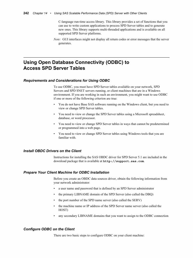
C-language run-time access library. This library provides a set of functions that you can use to write custom applications to process SPD Server tables and to generate new ones. This library supports multi-threaded applications and is available on all supported SPD Server platforms.
Note: GUI interfaces might not display all return codes or error messages that the server generates.
Using Open Database Connectivity (ODBC) to Access SPD Server Tables
Requirements and Considerations for Using ODBCTo use ODBC, you must have SPD Server tables available on your network, SPD Servers and SPD SNET servers running, or client machines that are in a Windows environment. If you are working in such an environment, you might want to use ODBC if one or more of the following criterion are true:
• You do not have Base SAS software running on the Windows client, but you need to view or change SPD Server tables.
• You need to view or change the SPD Server tables using a Microsoft spreadsheet, database, or word processor.
• You need to view or change SPD Server tables in ways that cannot be predetermined or programmed into a web page.
• You need to view or change SPD Server tables using Windows tools that you are familiar with.
Install OBDC Drivers on the ClientInstructions for installing the SAS OBDC driver for SPD Server 5.1 are included in the download package that is available at http://support.sas.com.
Prepare Your Client Machine for ODBC InstallationBefore you create an OBDC data sources driver, obtain the following information from your network administrator:
• a user name and password that is defined by an SPD Server administrator
• the primary LIBNAME domain of the SPD Server (also called the DBQ)
• the port number of the SPD name server (also called the SERV)
• the machine name or IP address of the SPD Server name server (also called the HOST)
• any secondary LIBNAME domains that you want to assign to the ODBC connection
Configure ODBC on the ClientThere are two basic steps to configure ODBC on your client machine:
242 Chapter 14 • Using SAS Scalable Performance Data (SPD) Server with Other Clients
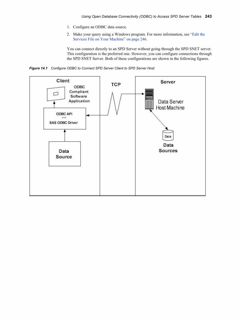
1. Configure an ODBC data source.
2. Make your query using a Windows program. For more information, see “Edit the Services File on Your Machine” on page 246.
You can connect directly to an SPD Server without going through the SPD SNET server. This configuration is the preferred one. However, you can configure connections through the SPD SNET Server. Both of these configurations are shown in the following figures.
Figure 14.1 Configure ODBC to Connect SPD Server Client to SPD Server Host
Using Open Database Connectivity (ODBC) to Access SPD Server Tables 243

Figure 14.2 Configure ODBC to Connect SPD Server Client to SPD SNET Server
Connecting to SPD Server Using an ODBC Connection
Primary and Secondary LIBNAME DomainsWhen a connection to the SPD server is established, a primary LIBNAME domain is assigned. The primary LIBNAME domain is specified by the DBQ connection options parameter. Immediately after the connection is made, the SAS ODBC driver assigns the secondary LIBNAME domains. You configure these domains on the Libraries tab of the SAS ODBC Driver Configuration window.
To make an ODBC connection through the SPD SNET server, you must configure an odbc.parm file on the SPD SNET Server machine.
Configure an ODBC Data Source to Connect Directly to an SPD ServerAfter you install the SAS ODBC driver, configure your ODBC data source. When you open the ODBC manager, enter information that points the OBDC driver to the data on the SPD Server.
1. From the Windows Start button, select Start ð Settings ð Control Panel.
2. Locate the ODBC Data Sources icon and open the Microsoft ODBC Data Source Administrator. The exact location of this program depends on your version of Windows.
3. Select the Add button, and then select the SAS ODBC driver.
4. Enter a data source name. You can also enter a description if you want to.
244 Chapter 14 • Using SAS Scalable Performance Data (SPD) Server with Other Clients

5. Select the Servers panel and enter your two-part server name.
6. Click the Configure box. In the TCP Options window, enter the following information:
Server AddressEnter the network address of the machine on which the SPD Server is running.
Server User NameEnter the user name as configured for a DBQ (an SPD Server primary LIBNAME domain) on the SPD Server to which you are connecting.
Server User PasswordEnter the user password as configured for a DBQ (an SPD Server primary LIBNAME domain) on the SPD Server host to which you are connecting.
Connection OptionsEnter values for the following options. Additional SPD Server LIBNAME options might be listed. For more information, see “SAS Scalable Performance Data (SPD) Server LIBNAME Options ” on page 173.
DBQ='SPD-Server-primary-LIBNAME-domain'the SPD Server LIBNAME domain
HOST='name-server-node-name'the location of the host computer
SERV='name-server-port-number'the port number of the SPD Server name server that is running on the host
7. Click OK. Click Add and select the Libraries panel.
8. Enter the DBQ name of a secondary LIBNAME domain in both the Name and Host File text fields.
9. Enter spdseng in the Engine text field.
10. Enter appropriate information in the Options text field. In this field. use SQL pass-through syntax rules for libref statements.
Configure an ODBC Data Source for SPD SNETAfter you install the SAS ODBC driver, configure your ODBC data source. When you open the ODBC manager, enter information that points the OBDC driver to the data on the SPD Server.
1. From the Windows Start button, select Start ð Settings ð Control Panel.
2. Click the ODBC icon and select the Add button.
3. Select the SAS ODBC driver.
4. Enter a data source name. You can also enter a description if you want to.
5. Select the Servers panel and enter your two-part server name. The second part of the server name should match the entry in the services file. For more information, see “Edit the Services File on Your Machine” on page 246. In that example, the server name is spdssnet.
6. Click the Configure box. In the TCP Options window, enter the following information:
Server AddressEnter the network address of the machine on which the SPD Server is running.
Using Open Database Connectivity (ODBC) to Access SPD Server Tables 245
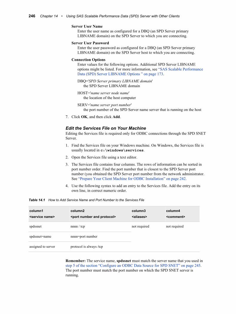
Server User NameEnter the user name as configured for a DBQ (an SPD Server primary LIBNAME domain) on the SPD Server to which you are connecting.
Server User PasswordEnter the user password as configured for a DBQ (an SPD Server primary LIBNAME domain) on the SPD Server host to which you are connecting.
Connection OptionsEnter values for the following options. Additional SPD Server LIBNAME options might be listed. For more information, see “SAS Scalable Performance Data (SPD) Server LIBNAME Options ” on page 173.
DBQ='SPD Server primary LIBNAME domain'the SPD Server LIBNAME domain
HOST='name server node name'the location of the host computer
SERV='name server port number'the port number of the SPD Server name server that is running on the host
7. Click OK, and then click Add.
Edit the Services File on Your MachineEditing the Services file is required only for ODBC connections through the SPD SNET Server.
1. Find the Services file on your Windows machine. On Windows, the Services file is usually located in c:\windows\services.
2. Open the Services file using a text editor.
3. The Services file contains four columns. The rows of information can be sorted in port number order. Find the port number that is closest to the SPD Server port number (you obtained the SPD Server port number from the network administrator. See “Prepare Your Client Machine for ODBC Installation” on page 242.
4. Use the following syntax to add an entry to the Services file. Add the entry on its own line, in correct numeric order.
Table 14.1 How to Add Service Name and Port Number to the Services File
column1
<service name>
column2
<port number and protocol>
column3
<aliases>
column4
<comment>
spdssnet nnnn / tcp not required not required
spdssnet=name nnnn=port number
assigned to server protocol is always /tcp
Remember: The service name, spdssnet must match the server name that you used in step 5 of the section “Configure an ODBC Data Source for SPD SNET” on page 245. The port number must match the port number on which the SPD SNET server is running.
246 Chapter 14 • Using SAS Scalable Performance Data (SPD) Server with Other Clients
Create a Query Using an ODBC-Compliant ProgramThe following instructions create a query using Microsoft Access.
1. Start the SPD SNET server.
2. Start Microsoft Access.
3. From the Microsoft Access main menu, select File ð Get External Table.
4. Select Link Table.
5. Select Files of Type.
6. Select ODBC Databases.
7. Select the data source.
Using JDBC (Java) to Access SPD Server Tables
Requirements and Considerations for Using JDBCTo use JDBC to access SPD Server tables, you must have SPD Server tables on the network, and SPD Server and SPD SNET servers must be running on the same server as the web server. If you are working in such an environment, you might want to use JDBC if one or more of the following criterion are true:
• You do not have Base SAS software on the network client to process the data sets.
• You want to distribute the information across your corporate intranet through a web page.
• The clients on your network are varied: UNIX machines, Windows PCs, and workstations.
• The audience for the information wants point-and-click access to it.
• You want to distribute the information over the Internet.
• Your planned application requires the power of the Java programming language.
Set Up JDBC Access to the ServerJDBC access to the server is performed through the SPD Server SNET process. Review your server start-up logs to verify that the spdssnet process is called and initialized.
Set Up JDBC on the ClientTo set up JDBC on the client, the client needs a browser that can accept Java applets.
Using JDBC (Java) to Access SPD Server Tables 247

Figure 14.3 JDBC Set Up on an SPD Server Client
Make a Query with JDBCTo use JDBC to make a query:
1. Open a browser and enter the URL for the web page that contains the JDBC code.
2. Click on the information that you are interested in. JDBC handles the request, formats the information, and returns the result to the web page.
HTML File Requirement for JDBCThe following lines must be part of the HTML file for JDBC:
<applet code="CLASSPATH.*.class codebase="../ width=600 height=425><param name=url value="jdbc:sharenet://spdssnet_node:PORT"><param name="dbms_options" value=DBQ='LIBNAME' HOST='host_node' SERV='NNNN'><param name="shareUser" value="userid"><param name="sharePassword" value="thepassword"><param name="shareRelease" value="V9"><param name="dbms" value="spds"></applet>
Line 1CLASSPATH points to the class path where the JDBC driver is installed.
248 Chapter 14 • Using SAS Scalable Performance Data (SPD) Server with Other Clients

*.class is the name of the Java class that consumes all of the <param name...> lines.
Line 2spdssnet_node is the node name of the machine on which the SPD SNET server is running.
PORT is the port number of the machine on which the SPD SNET server is running.
Line 3value=DBQ='LIBNAME' is the LIBNAME domain of the SPD Server.
HOST='host_node' is the location of the SPD SNET server.
SERV='NNNN' is the port number of the name server.
Line 4value=”userid” is the user ID that queries the SPD Server table.
Line 5value=”thepassword” is the password of the user ID that will make the query.
Line 6value=”V9” is the version of the driver that you are using. Do not modify this value.
Line 7Sets the foreign database property on the JDBC driver. If you specify a foreign database in line 7, the foreign database server does not need JDBC to create a SAS DataBaseMetaData object.
Limitations of Using JDBC with SPD Server
Using JDBC with SAS versus Using JDBC with SPD ServerSPD Server is treated as a foreign database. SPD Server clients cannot query the JDBC metadata class for available tables and other metadata. Users must write their own queries for these actions.
Example JDBC Query for Getting a List of TablesThe following example shows JDBC used with SPD Server:
SELECT '' AS qual,LIBNAME AS owner,MEMNAME AS name,MEMTYPE AS type,MEMNAME AS remarks FROM dictionary.tables AS tblWHERE ( memtype = 'DATA' OR memtype = 'VIEW' OR memtype = 'SYSTEM TABLE' OR memtype = 'ALIAS' OR memtype = 'SYNONYM')AND (tbl.LIBNAME NE 'MAPS' AND tbl.LIBNAME NE 'SASUSER' AND tbl.LIBNAME NE 'SASHELP')ORDER BY type, qual, owner, name
Example JDBC Query for Getting Metadata about a Specific TableThe following example shows using JDBC to query your data file for metadata:
SELECT '' AS qual,LIBNAME AS owner,MEMNAME AS tname, name,length AS datatype,
Using JDBC (Java) to Access SPD Server Tables 249
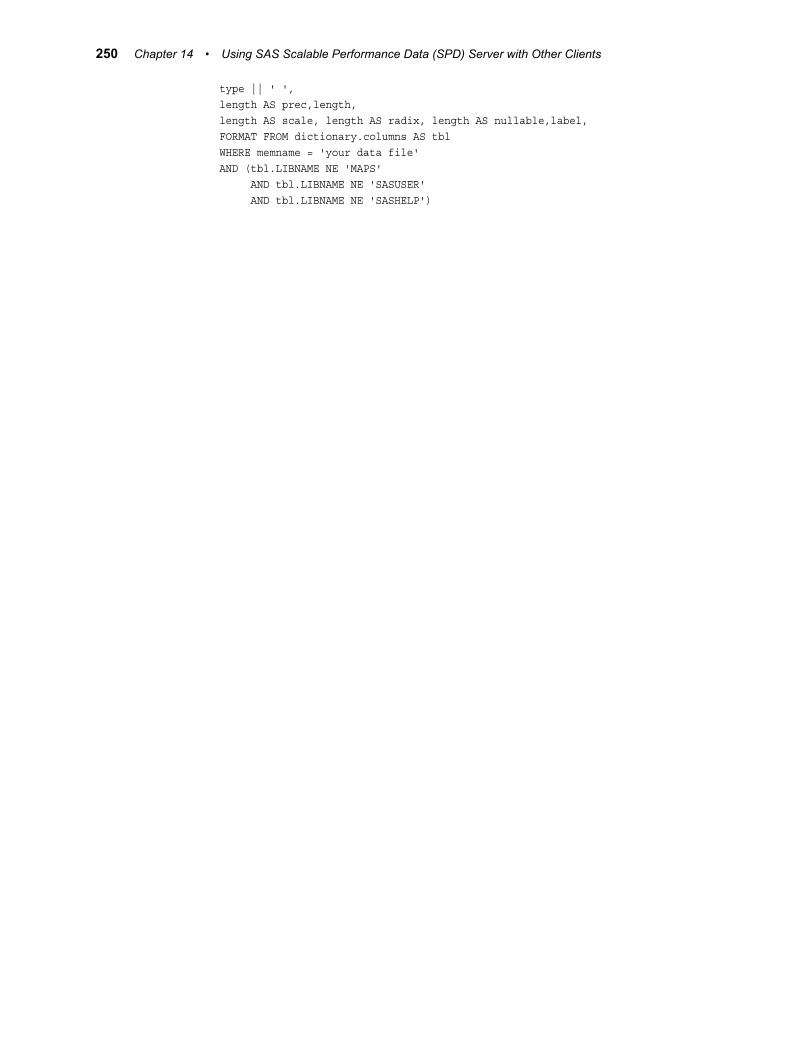
type || ' ',length AS prec,length,length AS scale, length AS radix, length AS nullable,label,FORMAT FROM dictionary.columns AS tblWHERE memname = 'your data file'AND (tbl.LIBNAME NE 'MAPS' AND tbl.LIBNAME NE 'SASUSER' AND tbl.LIBNAME NE 'SASHELP')
250 Chapter 14 • Using SAS Scalable Performance Data (SPD) Server with Other Clients

Chapter 15
SAS Scalable Performance Data (SPD) Server SQL Access Library API Reference
Introduction . . . . . . . . . . . . . . . . . . . . . . . . . . . . . . . . . . . . . . . . . . . . . . . . . . . . . . . . . 251
Overview of SPQL Usage . . . . . . . . . . . . . . . . . . . . . . . . . . . . . . . . . . . . . . . . . . . . . . 252
SPQL API Description . . . . . . . . . . . . . . . . . . . . . . . . . . . . . . . . . . . . . . . . . . . . . . . . 252
SPQL API Functions . . . . . . . . . . . . . . . . . . . . . . . . . . . . . . . . . . . . . . . . . . . . . . . . . 252spqlcolinfo() . . . . . . . . . . . . . . . . . . . . . . . . . . . . . . . . . . . . . . . . . . . . . . . . . . . . . . 252spqlconnect() . . . . . . . . . . . . . . . . . . . . . . . . . . . . . . . . . . . . . . . . . . . . . . . . . . . . . . 252spqldisconnect() . . . . . . . . . . . . . . . . . . . . . . . . . . . . . . . . . . . . . . . . . . . . . . . . . . . 253spqlfetch() . . . . . . . . . . . . . . . . . . . . . . . . . . . . . . . . . . . . . . . . . . . . . . . . . . . . . . . . 253spqlfreestok() . . . . . . . . . . . . . . . . . . . . . . . . . . . . . . . . . . . . . . . . . . . . . . . . . . . . . 254spqlgmsg() . . . . . . . . . . . . . . . . . . . . . . . . . . . . . . . . . . . . . . . . . . . . . . . . . . . . . . . 254spqlinit() . . . . . . . . . . . . . . . . . . . . . . . . . . . . . . . . . . . . . . . . . . . . . . . . . . . . . . . . . 254spqlperform() . . . . . . . . . . . . . . . . . . . . . . . . . . . . . . . . . . . . . . . . . . . . . . . . . . . . . 255spqltabinfo() . . . . . . . . . . . . . . . . . . . . . . . . . . . . . . . . . . . . . . . . . . . . . . . . . . . . . . 255spqlterm() . . . . . . . . . . . . . . . . . . . . . . . . . . . . . . . . . . . . . . . . . . . . . . . . . . . . . . . . 256
SPQL Function Return Codes . . . . . . . . . . . . . . . . . . . . . . . . . . . . . . . . . . . . . . . . . . 256SPQL_SUCCESS(==0) . . . . . . . . . . . . . . . . . . . . . . . . . . . . . . . . . . . . . . . . . . . . . 256SPQL_ENDDATA(WARNING) . . . . . . . . . . . . . . . . . . . . . . . . . . . . . . . . . . . . . . 256SPQL_INITFAILED(ERROR) . . . . . . . . . . . . . . . . . . . . . . . . . . . . . . . . . . . . . . . 256SPQL_NOMEM . . . . . . . . . . . . . . . . . . . . . . . . . . . . . . . . . . . . . . . . . . . . . . . . . . . 256SPQL_CONFAILED(ERROR) . . . . . . . . . . . . . . . . . . . . . . . . . . . . . . . . . . . . . . . 256SPQL_BADSTMT(ERROR) . . . . . . . . . . . . . . . . . . . . . . . . . . . . . . . . . . . . . . . . . 257
IntroductionThis chapter describes the Scalable Performance Data Server SQL access library API (Application Programming Interface) and provides some simple examples. This chapter refers to the Scalable Performance Data Server SQL access library as SPQL. Read this chapter if you want a library that provides a C-language compatible interface to write user applications to access an SPD Server SQL server. Because the library was designed for multi-threaded applications, the code is thread safe, except where noted in the following sections.
251
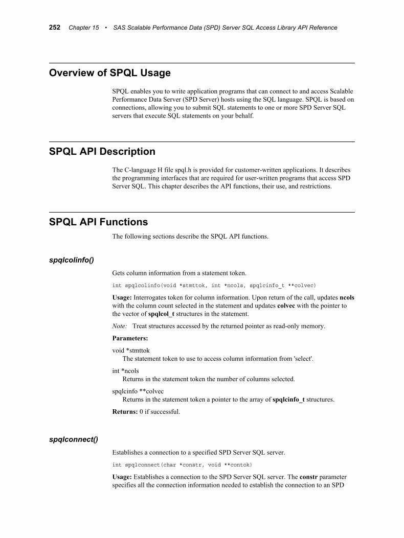
Overview of SPQL UsageSPQL enables you to write application programs that can connect to and access Scalable Performance Data Server (SPD Server) hosts using the SQL language. SPQL is based on connections, allowing you to submit SQL statements to one or more SPD Server SQL servers that execute SQL statements on your behalf.
SPQL API DescriptionThe C-language H file spql.h is provided for customer-written applications. It describes the programming interfaces that are required for user-written programs that access SPD Server SQL. This chapter describes the API functions, their use, and restrictions.
SPQL API FunctionsThe following sections describe the SPQL API functions.
spqlcolinfo()Gets column information from a statement token.
int spqlcolinfo(void *stmttok, int *ncols, spqlcinfo_t **colvec)
Usage: Interrogates token for column information. Upon return of the call, updates ncols with the column count selected in the statement and updates colvec with the pointer to the vector of spqlcol_t structures in the statement.
Note: Treat structures accessed by the returned pointer as read-only memory.
Parameters:
void *stmttokThe statement token to use to access column information from 'select'.
int *ncolsReturns in the statement token the number of columns selected.
spqlcinfo **colvecReturns in the statement token a pointer to the array of spqlcinfo_t structures.
Returns: 0 if successful.
spqlconnect()Establishes a connection to a specified SPD Server SQL server.
int spqlconnect(char *constr, void **contok)
Usage: Establishes a connection to the SPD Server SQL server. The constr parameter specifies all the connection information needed to establish the connection to an SPD
252 Chapter 15 • SAS Scalable Performance Data (SPD) Server SQL Access Library API Reference

Server SQL server. When a connection is made successfully, a connection, token (contok) is returned to the caller.
Parameters:
char *constrA null-terminated string identifying the SPD Server SQL server to connect to for this session. The syntax for the string is identical to that used for the SAS PROC SQL pass-through CONNECT statement. For more information about pass-through CONNECT statements, see “Specify SQL Options By Using Explicit Pass-Through Code” on page 71.
void **contokReturns a connection token if the connection successfully completes. You must retain the token; use it in subsequent SPQL library operations that you perform using the connection.
Returns: 0 if successful; SPQL_NOMEM if unable to allocate memory for the connection token; SPQL_CONFAILED if unable to connect successfully to the SPD Server SQL server.
spqldisconnect()Terminates a connection from the SPD Server SQL server specified with a spqlconnect().
int spqldisconnect(void *contok)
Usage: Disconnects from a specified SPD Server SQL server. The caller passes the connection token which was returned from an spqlconnect() call. Then, the SPD Server SQL server associated with the connection is disconnected from the caller, and the memory associated with connection token is returned to the system.
Parameters:
void *contokConnection token previously obtained from spqlconnect().
Returns: 0 if successful.
spqlfetch()Gets row data from a statement token.
int spqlfetch(void *stmttok, void **bufptr, int *bufsize)
Usage: Fetches each row that an executing statement returns. Each call to spqlfetch returns a row from a statement to the caller's buffer. If bufptr contains a NULL value, the routine returns a pointer to a buffer containing the next row. If the value is not NULL, it assumes that the buffer is owned by the caller and returns the data to the caller's buffer. In either case, bufsize is updated with the row length returned. Callers that use locate-mode spqlfetch semantics (that is, who specify bufptr as NULL), should NEVER FREE the memory pointer returned by spqlfetch. A call to spqlfetch(), after all rows for the statement are returned, returns a bufsize of 0.
Parameters:
void *stmttokThe statement token to use to access row data from the SELECT statement'.
SPQL API Functions 253

void **bufptrContains a pointer to the caller's row buffer to fill with row data. If it is NULL on entry, it returns a pointer to the internal result set buffer.
int *bufsizeReturns the size of the row buffer that was returned to the caller.
Returns: 0 if successful; SPQL_ENDDATA if the statement has no more rows to return; SPQL_FETCHFAILED if there is an unexpected failure while fetching the next row buffer.
spqlfreestok()
Frees resources used by a previously performed statement.
int spqlfreestok(void *stmttok);
Usage: Free resources used for the statement token from spqlperform(). Call spqlfreestok() after the data or information from the statement token has been extracted. You can call this function before all selected rows from the spqlperform() are read. If you do, the remaining unread rows (from the previous select) are discarded.
Parameters:
void *stmttokStatement token to free
Returns: 0 if successful.
spqlgmsg()Accesses thread-specific error or diagnostic message buffer contents.
int spqlgmsg(char **mbuf)
Usage: Returns a pointer to the threads error or diagnostic message buffer. Call spqlgmsg() to get any diagnostic messages if you encounter an error executing an SPQL function. If there is message information, spqlgmsg() returns the message pointer in the mbuf parameter as well as the length of the message (the function return value).
Parameters:
char **mbufReturns a pointer to the thread's error or diagnostic message buffer. If mbuf is NULL, there is no message information. The call also returns the length of the thread's error or diagnostic message buffer. A 0 indicates that no message exists.
spqlinit()Initializes the SPQL library for operation.
int spqlinit(void)
Usage: Performs a one-time initialization which enables the SPQL library to function. For this reason, you must call spqlinit() at least once to activate an SPQL program. Do not make other SPQL API calls before calling this function. If you do, the results are unpredictable. When spqlinit() successfully completes, you can safely proceed to use the SPQL API in a multi-threaded context.
254 Chapter 15 • SAS Scalable Performance Data (SPD) Server SQL Access Library API Reference
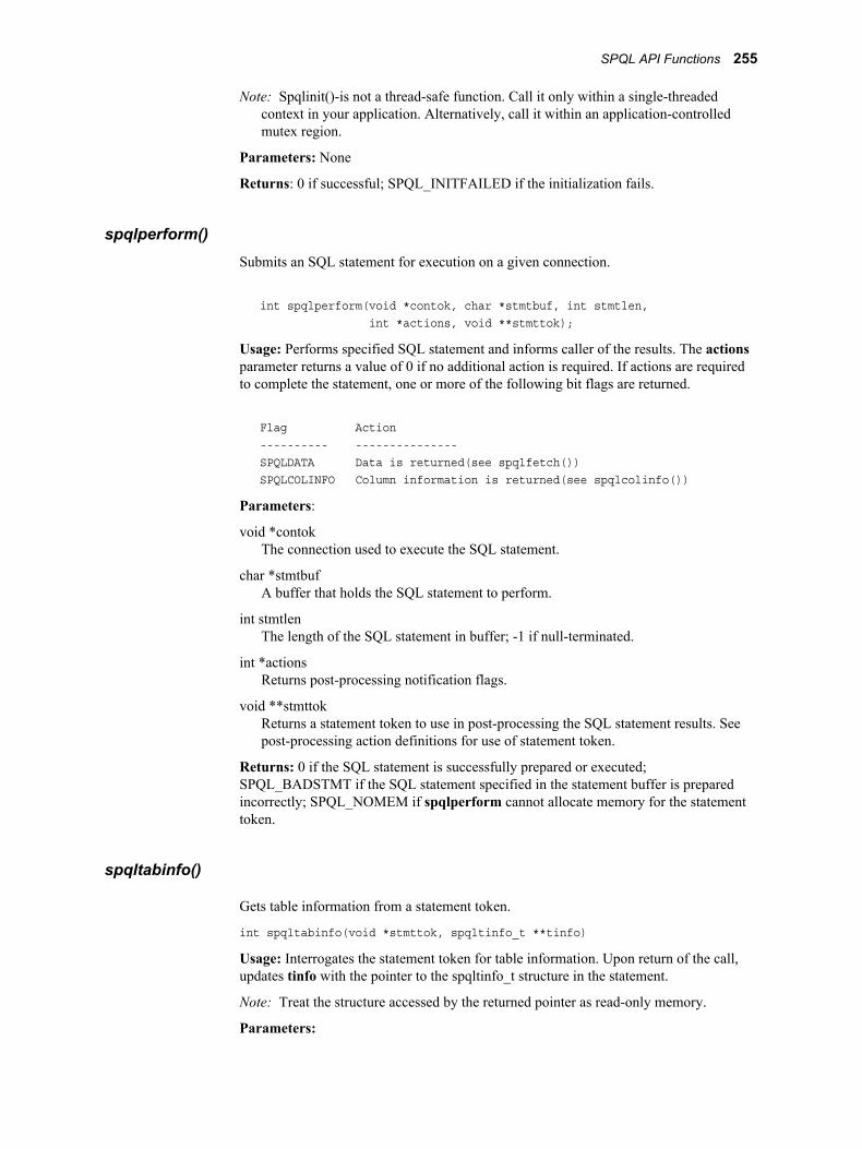
Note: Spqlinit()-is not a thread-safe function. Call it only within a single-threaded context in your application. Alternatively, call it within an application-controlled mutex region.
Parameters: None
Returns: 0 if successful; SPQL_INITFAILED if the initialization fails.
spqlperform()Submits an SQL statement for execution on a given connection.
int spqlperform(void *contok, char *stmtbuf, int stmtlen, int *actions, void **stmttok);
Usage: Performs specified SQL statement and informs caller of the results. The actions parameter returns a value of 0 if no additional action is required. If actions are required to complete the statement, one or more of the following bit flags are returned.
Flag Action ---------- --------------- SPQLDATA Data is returned(see spqlfetch()) SPQLCOLINFO Column information is returned(see spqlcolinfo())
Parameters:
void *contokThe connection used to execute the SQL statement.
char *stmtbufA buffer that holds the SQL statement to perform.
int stmtlenThe length of the SQL statement in buffer; -1 if null-terminated.
int *actionsReturns post-processing notification flags.
void **stmttokReturns a statement token to use in post-processing the SQL statement results. See post-processing action definitions for use of statement token.
Returns: 0 if the SQL statement is successfully prepared or executed; SPQL_BADSTMT if the SQL statement specified in the statement buffer is prepared incorrectly; SPQL_NOMEM if spqlperform cannot allocate memory for the statement token.
spqltabinfo()
Gets table information from a statement token.
int spqltabinfo(void *stmttok, spqltinfo_t **tinfo)
Usage: Interrogates the statement token for table information. Upon return of the call, updates tinfo with the pointer to the spqltinfo_t structure in the statement.
Note: Treat the structure accessed by the returned pointer as read-only memory.
Parameters:
SPQL API Functions 255

void *stmttokThe statement token to use to access table information from a 'select'.
spqltinfo **tinfoReturns pointer to spqltinfo_t structure into the statement token memory.
Returns: 0 for successful completion.
spqlterm()Is the termination counterpart of the spqlinit() function.
int spqlterm(void)
Usage: Terminates the SPQL library session, disconnecting all active SPD Server SQL server connections and freeing up the memory resources associated with the SPQL run-time library executables.
Parameters: None
Returns: 0 if successful.
SPQL Function Return CodesSome SPQL functions generate return codes, allowing you to check the value and take appropriate action in your application code. Typically, the application action taken upon receiving an error code is a call to spqlgmsg() to get the contents of the diagnostic buffer. The program can then display the buffer's contents to the user or write the contents to a log. The return codes in this section are classified by their state: positive [(WARNING), (SUCCESS)] or negative [(ERROR)].
SPQL_SUCCESS(==0)Successful completion of the SPQL function call.
SPQL_ENDDATA(WARNING)All rows selected were read from the statement token.
SPQL_INITFAILED(ERROR)Initialization failure. (It is unsafe for your application to make additional SPQL calls if this error occurs.)
SPQL_NOMEMUnable to allocate memory for some type of SPQL data structure. Check the diagnostic buffer for details.
SPQL_CONFAILED(ERROR)Unable to make a connection to an SPD Server SQL server. Check the diagnostic buffer for details.
256 Chapter 15 • SAS Scalable Performance Data (SPD) Server SQL Access Library API Reference

SPQL_BADSTMT(ERROR)SQL statement is incorrectly formatted for submission to sqlprepare(). Either the statement is blank (all white space) or contains contiguous non-white space characters.
SPQL Function Return Codes 257

258 Chapter 15 • SAS Scalable Performance Data (SPD) Server SQL Access Library API Reference
Part 5
SPD Server Appendices
Appendix 1SPD Server Advanced User Topics . . . . . . . . . . . . . . . . . . . . . . . . . . . . . . 261
Appendix 2SAS Scalable Performance Data (SPD) Server Frequently Asked Questions . . . . . . . . . . . . . . . . . . . . . . . . . . . . . . . . . . . . 287
Appendix 3SAS Scalable Performance Data (SPD) Server SQL Syntax Reference Guide . . . . . . . . . . . . . . . . . . . . . . . . . . . . . . . . . . . 305
Appendix 4SPD Server Supported SQL and WHERE-Processing Functions . . 319
259

260
Appendix 1
SPD Server Advanced User Topics
SPD Server Advanced User Topics . . . . . . . . . . . . . . . . . . . . . . . . . . . . . . . . . . . . . . 262
Accessing SPD Server through SAS . . . . . . . . . . . . . . . . . . . . . . . . . . . . . . . . . . . . . 262SQL Pass-Through Facility . . . . . . . . . . . . . . . . . . . . . . . . . . . . . . . . . . . . . . . . . . 262LIBNAME Access . . . . . . . . . . . . . . . . . . . . . . . . . . . . . . . . . . . . . . . . . . . . . . . . . 263SPD Server Host Name Server . . . . . . . . . . . . . . . . . . . . . . . . . . . . . . . . . . . . . . . . 264Specifying the Port Address for the Name Server . . . . . . . . . . . . . . . . . . . . . . . . . 264
Organizing SAS Data . . . . . . . . . . . . . . . . . . . . . . . . . . . . . . . . . . . . . . . . . . . . . . . . . 265SPD Server Tables . . . . . . . . . . . . . . . . . . . . . . . . . . . . . . . . . . . . . . . . . . . . . . . . . 265SPD Server Component Files . . . . . . . . . . . . . . . . . . . . . . . . . . . . . . . . . . . . . . . . . 265SPD Server Table Indexes . . . . . . . . . . . . . . . . . . . . . . . . . . . . . . . . . . . . . . . . . . . 267
SPD Server Performance Enhancements . . . . . . . . . . . . . . . . . . . . . . . . . . . . . . . . . 267SPD Server Pass-Through SQL Enhancements . . . . . . . . . . . . . . . . . . . . . . . . . . . 267Implicit and Explicit Server Sorts . . . . . . . . . . . . . . . . . . . . . . . . . . . . . . . . . . . . . . 267Modified SAS Heap Sort . . . . . . . . . . . . . . . . . . . . . . . . . . . . . . . . . . . . . . . . . . . . 267Indexed Parallel Table Scan . . . . . . . . . . . . . . . . . . . . . . . . . . . . . . . . . . . . . . . . . . 267Improved Table Appends . . . . . . . . . . . . . . . . . . . . . . . . . . . . . . . . . . . . . . . . . . . . 268
Using SPD Server with Data Warehousing . . . . . . . . . . . . . . . . . . . . . . . . . . . . . . . 268
SPD Server Macro Variables . . . . . . . . . . . . . . . . . . . . . . . . . . . . . . . . . . . . . . . . . . . 270Overview of Macro Variables . . . . . . . . . . . . . . . . . . . . . . . . . . . . . . . . . . . . . . . . 270
Using a LIBNAME to Statement to Access SPD Server . . . . . . . . . . . . . . . . . . . . . 270The Client Session . . . . . . . . . . . . . . . . . . . . . . . . . . . . . . . . . . . . . . . . . . . . . . . . . 270
Managing Large SPD Server Files . . . . . . . . . . . . . . . . . . . . . . . . . . . . . . . . . . . . . . 272Initial Setup of SPD Server LIBNAME Domain Storage . . . . . . . . . . . . . . . . . . . 272Effect of the Administrator Option ROPTIONS= . . . . . . . . . . . . . . . . . . . . . . . . . 272Using Explicit or Default Storage Paths . . . . . . . . . . . . . . . . . . . . . . . . . . . . . . . . . 273SPD Server Component Storage . . . . . . . . . . . . . . . . . . . . . . . . . . . . . . . . . . . . . . . 274Forced Partitioning of the Data Component . . . . . . . . . . . . . . . . . . . . . . . . . . . . . . 275Using Path Options for Large Table Storage . . . . . . . . . . . . . . . . . . . . . . . . . . . . . 276
Indexing SPD Server Tables . . . . . . . . . . . . . . . . . . . . . . . . . . . . . . . . . . . . . . . . . . . 277The SPD Server Index . . . . . . . . . . . . . . . . . . . . . . . . . . . . . . . . . . . . . . . . . . . . . . 277
SPD Server Join Planner . . . . . . . . . . . . . . . . . . . . . . . . . . . . . . . . . . . . . . . . . . . . . . 278
SPD Server Join Planner Examples . . . . . . . . . . . . . . . . . . . . . . . . . . . . . . . . . . . . . 279Join Planner DETAILS= Reset Switch Examples . . . . . . . . . . . . . . . . . . . . . . . . . 279Using JOINTECH_PREF Reset Switch to Alter an Index Join to a Hash Join . . . 279N-Way Join Example . . . . . . . . . . . . . . . . . . . . . . . . . . . . . . . . . . . . . . . . . . . . . . . 280
SPD Server STARJOIN Optimization . . . . . . . . . . . . . . . . . . . . . . . . . . . . . . . . . . . 281
261
Overview of STARJOIN Optimization . . . . . . . . . . . . . . . . . . . . . . . . . . . . . . . . . 281Enabling STARJOIN Optimization in SPD Server . . . . . . . . . . . . . . . . . . . . . . . . 282Classify Dimension Tables That Are Called by SQL as Phase
I Tables or Phase II Tables . . . . . . . . . . . . . . . . . . . . . . . . . . . . . . . . . . . . . . . . . 282Phase I Probes Fact Table Indexes and Selects a STARJOIN Strategy . . . . . . . . . 282Phase II Performs Index Lookups and Joins Subsetted Fact
Table Rows with Phase II Tables . . . . . . . . . . . . . . . . . . . . . . . . . . . . . . . . . . . . 285
SPD Server Advanced User TopicsThis appendix contains information and detailed examples about advanced SPD Server topics that typical users are unlikely to encounter. Certain power users and SPD Server Administrators might find additional information (such as server architecture illustrations and detailed examples for special-use cases) useful when special circumstances or user configurations require some of the less-commonly used SPD Server software functions.
Accessing SPD Server through SASYou begin an SPD Server session by starting your SPD Server client. You can use SQL commands to start your SPD Server client session, or you can use a LIBNAME statement. Both methods use the sasspds engine and initiate communication between the SPD Server client machine and the SPD Server host.
SQL Pass-Through FacilitySAS can execute SQL commands within the client, or pass the SQL to the server. SPD Server supports SQL that is passed to it from the client. The SPD Server host can completely evaluate SQL expressions. SPD Server also supports nested SQL pass-through commands. You can use SQL pass-through commands to connect to other SPD Server hosts while you are connected to your SPD Server host. You can use nested pass-through commands to distribute simultaneous SQL queries across multiple SPD Server hosts on your network.
You can access the SQL pass-through facility with or without SAS syntax and applications. You can use SAS to connect to an SPD Server host by using pass-through syntax from PROC SQL or from other SQL-aware SAS applications. For more information about the SPD Server pass-through facility and for syntax examples, see “Accessing and Creating SAS Scalable Performance Data (SPD) Server Tables” on page 19.
262 Appendix 1 • SPD Server Advanced User Topics
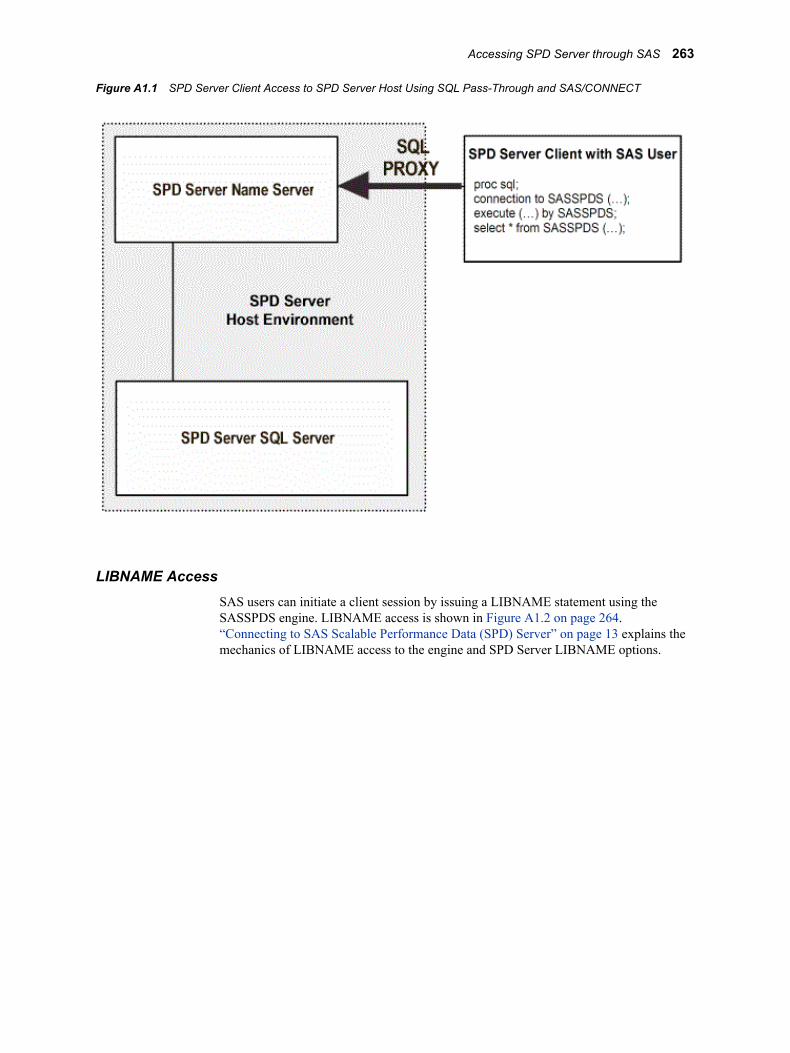
Figure A1.1 SPD Server Client Access to SPD Server Host Using SQL Pass-Through and SAS/CONNECT
LIBNAME AccessSAS users can initiate a client session by issuing a LIBNAME statement using the SASSPDS engine. LIBNAME access is shown in Figure A1.2 on page 264. “Connecting to SAS Scalable Performance Data (SPD) Server” on page 13 explains the mechanics of LIBNAME access to the engine and SPD Server LIBNAME options.
Accessing SPD Server through SAS 263

Figure A1.2 SPD Server Client Access (SAS User) to SPD Server Host Using a LIBNAME Statement
SPD Server Host Name ServerDistributed computing can enrich user resources, but in order to connect to an SPD Server, you must know its location within your network. Instead of requiring users to memorize long paths or IP addresses, SPD Server software uses a specialized server called a name server. The SPD Server name server locates active SPD Server hosts on your network. A name server recognizes active SPD Server machines because all of the SPD Servers register with the name server as they start and contact the host machine.
The name server keeps network addresses and a list of the LIBNAME domains for each SPD Server host. An SPD Server LIBNAME domain is a logical entity that SPD Server creates. A LIBNAME domain maintains domain attributes such as the library name, owner, and contents. Whenever you use a LIBNAME statement to specify a LIBNAME domain, a name server can determine the correct directory path to the SPD Server data library and connect your SPD Server client to the SPD Server host for that domain.
Specifying the Port Address for the Name ServerSPD Server clients use port addresses to locate an SPD Server name server. SPD Server administrators must assign a port address to a name server. Most UNIX system clients use their local /etc/services file to register port assignments. The service name for an SPD Server name server in an /etc/services file must be SPDSNAME. PC clients use services files to register port assignments. The services files on PC clients vary based on the software that the PC network uses.
When a client SPD Server application issues a LIBNAME statement that does not include the port address of the name server, SPD Server checks the services file for the
264 Appendix 1 • SPD Server Advanced User Topics
SPDSNAME entry and the port address. If you register the name server port assignment in your client's network services file, you will not have to code name server port numbers when you write SAS jobs. For examples of how to use a LIBNAME statement to connect to the host, see “Examples of the LIBNAME Statement” on page 18.
Organizing SAS Data
SPD Server TablesSPD Server software alters SAS tables to enable high-performance processing. SPD Server tables are physically different from a Base SAS table. You can use tables in either SAS or native SPD Server format. For more information about how to migrate tables between SAS and SPD Server, see “Migrating Tables between SAS and SPD Server” on page 22.
SAS tables store a single file that contains the data descriptors and the table data. The data are column values. The descriptors are metadata that describe the column and data formatting that the table uses.
SPD Server tables do not reuse space. When an SQL command to delete one or more rows from a table is issued, the row is marked deleted and the space is not reused. You must copy the table in order to recapture the space.
Figure A1.3 on page 266 shows differences in the architecture between SPD Server tables and SAS tables. SPD Server uses component files to store tables. One component file stores the stream of data values. Another component file stores the column and data descriptors. If you create an index for a column or a composite of columns, SPD Server creates component files for each index.
SPD Server Component FilesFigure A1.3 on page 266 shows the components of SPD Server tables.
Organizing SAS Data 265

Figure A1.3 SPD Server Component Files
SPD Server uses four types of component files to store SPD Server tables.
These two component files store table information:
*.dpfstores a stream of the table's data values.
*.mdfstores the table's metadata.
These two component files manage index data:
*.hbxunique global B-tree indexes.
*.idxsegmented views of the indexed column data. The *.idx components are useful when you are evaluating parallel WHERE clauses.
SPD Server partitions component files when they are created to prevent the files from growing too large. SPD Server stores each partitioned component file as one or more disk files. The partitioning provides the following advantages:
• Support for very large tables: SPD Server bypasses the file size limits that are imposed by many applications and operating systems. By using partitioned component files, SPD Server can support any file system transparently.
• Access via multiple directory paths: SPD Server can access data libraries that span numerous directory paths and storage devices. SPD Server software partitions massive data libraries into component files. The component architecture enables rapid, threaded data access, and circumvents device capacity and file size limitation
266 Appendix 1 • SPD Server Advanced User Topics
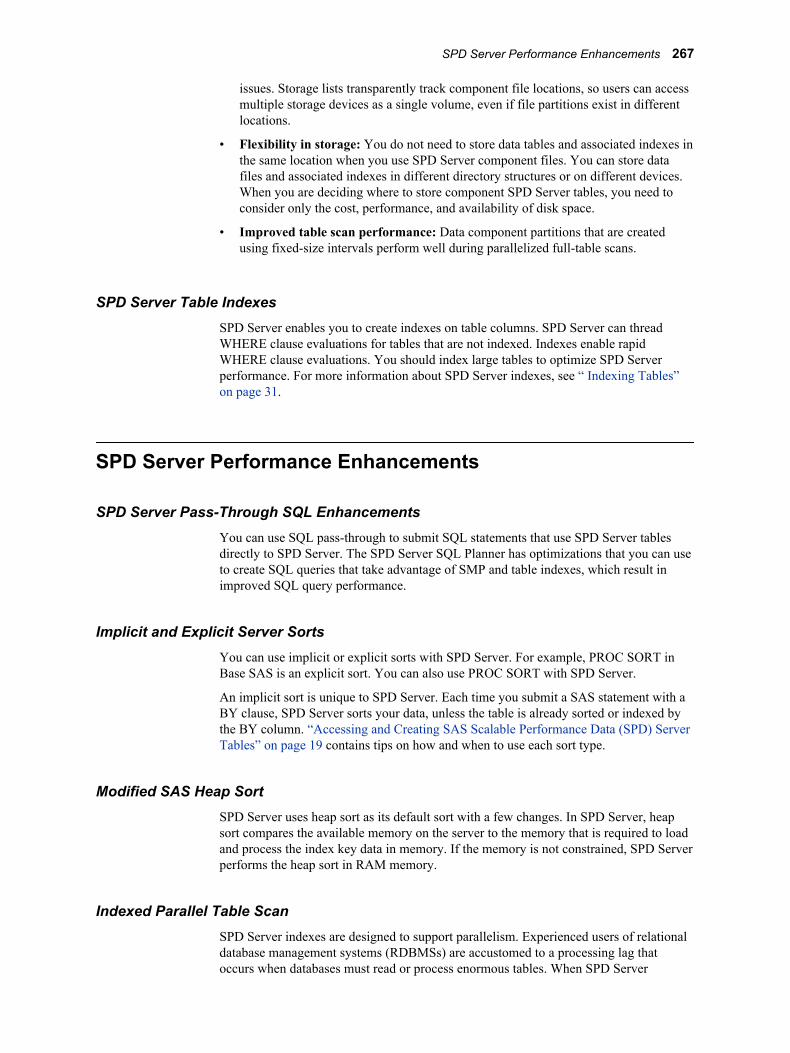
issues. Storage lists transparently track component file locations, so users can access multiple storage devices as a single volume, even if file partitions exist in different locations.
• Flexibility in storage: You do not need to store data tables and associated indexes in the same location when you use SPD Server component files. You can store data files and associated indexes in different directory structures or on different devices. When you are deciding where to store component SPD Server tables, you need to consider only the cost, performance, and availability of disk space.
• Improved table scan performance: Data component partitions that are created using fixed-size intervals perform well during parallelized full-table scans.
SPD Server Table IndexesSPD Server enables you to create indexes on table columns. SPD Server can thread WHERE clause evaluations for tables that are not indexed. Indexes enable rapid WHERE clause evaluations. You should index large tables to optimize SPD Server performance. For more information about SPD Server indexes, see “ Indexing Tables” on page 31.
SPD Server Performance Enhancements
SPD Server Pass-Through SQL EnhancementsYou can use SQL pass-through to submit SQL statements that use SPD Server tables directly to SPD Server. The SPD Server SQL Planner has optimizations that you can use to create SQL queries that take advantage of SMP and table indexes, which result in improved SQL query performance.
Implicit and Explicit Server SortsYou can use implicit or explicit sorts with SPD Server. For example, PROC SORT in Base SAS is an explicit sort. You can also use PROC SORT with SPD Server.
An implicit sort is unique to SPD Server. Each time you submit a SAS statement with a BY clause, SPD Server sorts your data, unless the table is already sorted or indexed by the BY column. “Accessing and Creating SAS Scalable Performance Data (SPD) Server Tables” on page 19 contains tips on how and when to use each sort type.
Modified SAS Heap SortSPD Server uses heap sort as its default sort with a few changes. In SPD Server, heap sort compares the available memory on the server to the memory that is required to load and process the index key data in memory. If the memory is not constrained, SPD Server performs the heap sort in RAM memory.
Indexed Parallel Table ScanSPD Server indexes are designed to support parallelism. Experienced users of relational database management systems (RDBMSs) are accustomed to a processing lag that occurs when databases must read or process enormous tables. When SPD Server
SPD Server Performance Enhancements 267
performs table queries, the SPD Server index architecture enables the software to analyze different table sections or segments in parallel. By processing large table segments in parallel, SPD Server delivers much faster data throughput. The faster throughput might be difficult to perceive on small tables, but when SPD Server performs scans on very large tables, the processing performance is significantly faster than that of database systems that support only serial indexed table scans.
Improved Table AppendsSPD Server separates the Table Append operation into steps that can be performed in parallel. The level of parallelism depends on the number of indexes in the table. The more indexes you have, the greater the potential of exploiting parallelism during the append.
T I P You can save time by creating an empty table in SPD Server, defining your indexes on it, and then appending the data. It is faster to create indexes on an empty table than it is to load the table, and then create the indexes.
Using SPD Server with Data WarehousingSPD Server offers data warehouse users an excellent facility to store data. SPD Server uses component files and partitioning to alleviate large table constraints such as device or directory size limits. SPD Server can perform storage services on a reliable and relatively inexpensive machine.
In addition to providing efficient, economical storage, SPD Server can deliver the enhanced processing capabilities users need to manage and query data in a warehouse. SMP processing provides the power to parallel-process huge tables. SPD Server offers multiple access, domain protection, and table locking. These features enable data warehouse users to secure and access their shared SPD Server.
268 Appendix 1 • SPD Server Advanced User Topics

Figure A1.4 Data Warehouse with Large Data Stores
Several data stores (repositories for data) are contained in a data warehouse. Three stores are of interest in the previous figure: detail tables, summary tables, and data marts. Organizations often store transactions that are up to 90 days old in a detail table, transactions that are up to a year old in a summary table, and additional data snapshots in data marts.
To perform queries, data warehouse users can use SAS with SAS syntax or PROC SQL syntax. Alternatively, SPD Server supports the use of other vendor applications that use SQL pass-through and that comply with other connection standards that SAS does not comply with. SPD Server can contribute significantly to the objectives of a data warehouse: to deliver low-cost, relevant, machine-independent, and timely information to users throughout the organization.
Using SPD Server with Data Warehousing 269
SPD Server Macro Variables
Overview of Macro VariablesYou can use global macro variables in SPD Server to simplify your work. Global macro variables use default values that are set by SPD Server and that operate in the background. You can make global changes to the values of macro variables in your code by specifying a new default setting for the specified variable. The new default setting is applied to all macro variables in the code that you submit to SPD Server. You can override the setting for a single macro variable by using a table option to change the setting for only the specified table.
The default macro variable values automate processing decisions. The default settings provide good performance. However, optimal performance requires changes to the default settings of some macro variables. Before you make changes to the default settings, consider conducting performance testing first. After you quantify performance parameters by using several macro variable settings, you can customize SPD Server so that it solves your business or data problems with maximum efficiency.
Each SPD Server installation is different. You might want to change many values, or just a few. Either way, macro variables are flexible and easy to manipulate.
Use a %LET statement to change macro variable values. You can place the macro variable assignment anywhere in the open code of a SAS program except in the data lines. The most convenient location for your %LET statements to initialize macro variables is in your autoexec.sas file or at the beginning of a program. The macro variable assignment is valid for the duration of your session or the executing program. Macro variable values remain in effect until they are changed by a subsequent assignment.
Assignments for macro variables with YES or NO arguments must be uppercase.
Because SPD Server macro variables operate behind the scenes, you cannot query SPD Server to determine the status of a macro variable. SAS does not know about the status of macro variables. If you want to know which SPD Server macro variables are in effect, or what their default values are, you can use PROC SPDO.
For detailed information about using SPD Server Macro Variables, see “SAS Scalable Performance Data (SPD) Server Macro Variables ” on page 152.
Using a LIBNAME to Statement to Access SPD Server
The Client SessionSuccessfully issuing the LIBNAME statement or SQL pass-through statements initiates an SPD Server client session. The client session operates using a combination of the following four components.
SPD Server name serverThe name server acts like a traffic cop and serves as command central between clients and SPD Server hosts. The name server maintains a list of LIBNAME
270 Appendix 1 • SPD Server Advanced User Topics

domains associated with each SPD Server host. Client sessions always connect to an SPD Server host through a name server. The name server resolves the submitted LIBNAME domain name (a logical entity) to a physical path (usually a UNIX or Windows directory). The name server connects you to the SPD Server that servers the domain without requiring you to know physical addresses. An SPD Server administrator sets up the LIBNAME domains in a parameter file for SPD Server, which then registers its domains with the name server.
SPD Server hostEach SPD Server host controls security access to the domain resources that it manages. When an SPD Server host starts, it registers its LIBNAME domains with the name server. Clients can connect to an SPD Server host only through a name server. Direct connections between clients and SPD Server hosts are not permitted. The SPD Server host validates the client user ID and password (passed in the LIBNAME statement), launches the system process (client proxy) for each client, and grants access to the appropriate SPD Server domain.
SQL serverThe SQL server parses and processes the SQL pass-through syntax submitted by the SAS client.
SPDSSNET serverThe SPDSSNET server enables access between clients without SAS and SPD Server. The SPDSSNET server runs as a stand-alone process on either the client or SPD Server host machine. It acts as a bridge between the SAS ODBC driver and the SPD Server host. You can use SPDSSNET with JDBC drivers and with htmSQL drivers. SPDSSNET can run multiple processes concurrently and perform parallel processing.
Figure A1.5 SPD Server Hosts, SPD Server Name Servers, and LIBNAME Domains
Using a LIBNAME to Statement to Access SPD Server 271

Managing Large SPD Server FilesManaging large files is not only a performance issue; it also has implications for file storage and disk space. Optimally, an SPD Server administrator manages storage space for SPD Server LIBNAME domains. In that case, you do not need to consider storage issues. SPD Server does the work for you. “Optimizing SAS Scalable Performance Data Server (SPD) Server ” on page 120 contains more information about managing large SPD Server files.
Initial Setup of SPD Server LIBNAME Domain StorageThe figure below shows how an SPD Server domain is set up. An SPD Server administrator must define the name and primary path for the domain in the LIBNAME parameter file for SPD Server. The path that the administrator defines for each domain is referred to as the primary file system for that domain. SPD Server reads the LIBNAME parameter file at start-up. The SPD Server registers the domains with the SPD Server name server. When the user issues a LIBNAME statement, the client sends a message to the SPD Server name server that resolves the domain name to its physical directory path, and the client determines the SPD Server that registered the domain.
Figure A1.6 SPD Server LIBNAME Domains
Effect of the Administrator Option ROPTIONS=After an SPD Server administrator defines a primary file system for a domain, the administrator can use LIBNAME parameter file options, identical to the DATAPATH=, METAPATH=, and INDEXPATH= options in the LIBNAME statement, to set up additional paths for the domain. However, the administrator can restrict a user from defining additional paths using the LIBNAME statement with the ROPTIONS= LIBNAME parameter file option. When an SPD Server administrator uses the ROPTIONS= option, the administrator's specification takes precedence over the user's
272 Appendix 1 • SPD Server Advanced User Topics

specification. For more information, see “Configuring LIBNAME Domain Disk Space” in Chapter 10 of SAS Scalable Performance Data Server: Administrator's Guide.
For example, assume that a user uses the DATAPATH= option to specify a path to store table data for a domain. If the SPD Server administrator also uses the DATAPATH= option with ROPTIONS= for that domain entry in the LIBNAME parameter file, the user's DATAPATH= specifications are ignored.
When the administrator uses ROPTIONS= with path options, users are relieved of the complicated task of managing disk space. Moreover, path information does not need to be embedded in SAS programs. Instead, SAS jobs refer to only the logical LIBNAME and rely on ROPTIONS= embedded by the administrator to specify all of the physical path information. This approach uses the power of the name server and lets it resolve path information for an SPD Server domain.
Using Explicit or Default Storage PathsThe first LIBNAME assignment or SQL pass-through CONNECT statement that names a domain establishes an initial set of paths for the domain. You can explicitly specify the paths and manage your own disk space, or the software can establish a default set of paths. The best choice is to use the default paths. The following figure shows primary file system default paths:
Figure A1.7 Primary File System Default Paths
Figure A1.8 on page 274 shows an explicit initial set of paths.
Managing Large SPD Server Files 273
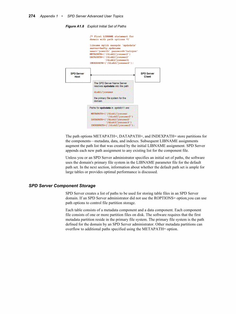
Figure A1.8 Explicit Initial Set of Paths
The path options METAPATH=, DATAPATH=, and INDEXPATH= store partitions for the components—metadata, data, and indexes. Subsequent LIBNAME assignments augment the path list that was created by the initial LIBNAME assignment. SPD Server appends each new path assignment to any existing list for the component file.
Unless you or an SPD Server administrator specifies an initial set of paths, the software uses the domain's primary file system in the LIBNAME parameter file for the default path set. In the next section, information about whether the default path set is ample for large tables or provides optimal performance is discussed.
SPD Server Component StorageSPD Server creates a list of paths to be used for storing table files in an SPD Server domain. If an SPD Server administrator did not use the ROPTIONS= option,you can use path options to control file partition storage.
Each table consists of a metadata component and a data component. Each component file consists of one or more partition files on disk. The software requires that the first metadata partition reside in the primary file system. The primary file system is the path defined for the domain by an SPD Server administrator. Other metadata partitions can overflow to additional paths specified using the METAPATH= option.
274 Appendix 1 • SPD Server Advanced User Topics
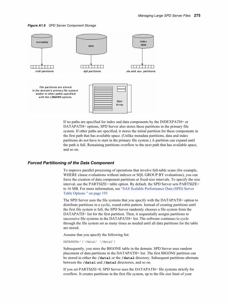
Figure A1.9 SPD Server Component Storage
If no paths are specified for index and data components by the INDEXPATH= or DATAPATH= options, SPD Server also stores these partitions in the primary file system. If other paths are specified, it stores the initial partition for these components in the first path that has available space. (Unlike metadata partitions, data and index partitions do not have to start in the primary file system.) A partition can expand until the path is full. Remaining partitions overflow to the next path that has available space, and so on.
Forced Partitioning of the Data ComponentTo improve parallel processing of operations that involve full-table scans (for example, WHERE clause evaluations without indexes or SQL GROUP BY evaluations), you can force the creation of data component partitions at fixed-size intervals. To specify the size interval, use the PARTSIZE= table option. By default, the SPD Server sets PARTSIZE= to 16 MB. For more information, see “SAS Scalable Performance Data (SPD) Server Table Options ” on page 193
The SPD Server uses the file systems that you specify with the DATAPATH= option to distribute partitions in a cyclic, round-robin pattern. Instead of creating partitions until the first file system is full, the SPD Server randomly chooses a file system from the DATAPATH= list for the first partition. Then, it sequentially assigns partitions to successive file systems in the DATAPATH= list. The software continues to cycle through the file system set as many times as needed until all data partitions for the table are stored.
Assume that you specify the following list:
DATAPATH='('/data1' '/data2')
Subsequently, you store the BIGONE table in the domain. SPD Server uses random placement of data partitions in the DATAPATH= list. The first BIGONE partition can be stored in either the /data1 or the /data2 directory. Subsequent partitions alternate between the /data1 and /data2 directories, and so on.
If you set PARTSIZE=0, SPD Server uses the DATAPATH= file systems strictly for overflow. It creates partitions in the first file system, up to the file size limit of your
Managing Large SPD Server Files 275
operating system. When the first file system is full, it proceeds to the second file system, and so on.
What happens when you issue the first LIBNAME statement for a domain, but you do not specify path options? If your tables are small, the primary file system is probably adequate. However, if your tables are large, the primary file system can fill up quickly. When the primary file system is full, SPD Server returns an error message when you perform an Append operation on an existing table, or when you create a new table in the domain.
If the primary file system is full, you can issue a subsequent LIBNAME statement that specifies additional paths. You can append to an existing table, but you might not be able to create a new table in the domain. The software cannot store the first metadata file partition because the primary file system is still full. What is the solution? You need to either free space in the primary file system or get the SPD Server administrator to create a new LIBNAME domain.
Using Path Options for Large Table Storage
Overview of Using Path OptionsIf you must manage your table storage, anticipate disk space for large tables. Use the LIBNAME path options with the first LIBNAME statement for the domain. To store data and index partitions, use the DATAPATH= and INDEXPATH= options on a different storage device other than the primary file system. By using a different storage device, you reserve the primary file system for metadata files.
Scenario for Using Path OptionsIn this example, the SPD Server administrator has already created the primary file system for MYLIB.
1. Specify an explicit initial set of paths.
SITEUSR1 issues the first LIBNAME statement for the MYLIB domain. By default, the domain's primary file system is used to store metadata partitions. SITEUSR1 specifies another device (MYDISK30) and directory (SITEUSER) to store the data and index partitions.
/* I anticipate the primary file system for the MYLIB domain */ /* is ample for metadata files, but I will use MYDISK30 */ /* to store my data and index partitions. */ LIBNAME myref sasspds 'mylib' datapath=('/mydisk30/siteuser') indexpath=('/mydisk30/siteuser') server=husky.spdsname user='siteusr1' prompt=yes;
2. Specify a subsequent LIBNAME statement to add paths.
SITEUSR1 issues a subsequent LIBNAME statement for the MYLIB domain and specifies additional paths for the data and index partitions. The user is storing large tables, so the list specifies two storage devices and directories for the data. SITEUSR1 also specifies a third device for indexes that are associated with the tables.
/* I noticed today MYDISK30 is getting full. */ /* I am adding MYDISK31 for possible overflow. */
276 Appendix 1 • SPD Server Advanced User Topics
LIBNAME expand sasspds 'mylib' datapath=('/mydisk31/siteuser' '/mydisk32/siteuser') indexpath=('/mydisk33/siteuser') server=husky.spdsname user='siteusr1' prompt=yes;
3. Append the new paths to the existing list for each component type. The following path list is maintained by spdslibll:
datapath=('mydisk30/siteuser' '/mydisk31/siteuser' '/mydisk32/siteuser')indexpath=('mydisk30/siteuser' '/mydisk33/siteuser')
SPD Server stores partitions of the data components for MYLIB tables in the specified data paths. (How the software uses the data paths depends on the value of the PARTSIZE= option.) For index components, SPD Server stores partitions in the first path in the list until that space is full, and then it proceeds to the next path in the list.
Indexing SPD Server TablesSPD Server efficiently indexes tables of varying size and data distributions. The SPD Server SPD index supports queries that require global table views (such as queries that contain BY clause processing or SQL joins), or queries that require segmented views (such as parallel processing of WHERE clause statements).
The SPD Server IndexThe SPD Server index maintains two views of the index values: a global view and a segmented view. SPD Server maintains the global view by using a unique global B-tree that has a single entry for each discrete value. The segmented view is maintained by the data for each value in the global B-tree, which includes a list of segments that contain the value, and includes for each segment a bitmap that identifies which rows in the segment contain the value. The global view is maintained in the SPD Server index.hbx file, and the segmented data is maintained in the SPD Server index.idx file.
For queries that require a global view, SPD Server searches the hybrid global B-tree for a particular value. SPD Server scans the segment lists for the value, and then reads the bitmaps from each segment that contains the value. SPD Server uses the bitmap to locate and retrieve the observations for that segment. This type of query returns results sorted first by value and then by observation number. This sorting is optimal for BY clause processing and SQL joins.
A parallel WHERE clause on a table that is indexed is done in two phases. The first phase, pre-evaluation, uses the SPD Server indexes to build a list of segments that satisfy the query. The list drops segments from the WHERE clause scan queue when those segments contain no data in the clause range. As more and more segments are excluded from the scan queue, the benefit of the pre-evaluation phase increases proportionally. The second phase in the evaluation launches threads that read an index in parallel. Each thread queries a particular segment of the index, using information from the pre-evaluation phase. The thread uses the SPD Server index to read the segment bitmap. The per-segment bitmaps identify the segment rows that satisfy the query for that particular
Indexing SPD Server Tables 277
column. If you include more than one indexed column in the WHERE clause, SPD Server retrieves the per-segment bitmaps for each column in parallel (as are the segments for each column). After SPD Server retrieves all the bitmaps for each column of the segment, it determines which rows satisfy the query and returns those segment rows to the client. The multi-threaded per-segment queries begin execution at the same time, but their finishing order varies and cannot be reasonably predicted. As a result, the overall order of the results cannot be guaranteed when you are using this type of query. For more information about using indexed columns with WHERE clause evaluations, see “WHERE Clause Planner” on page 133 .
When a table is modified as the result of an append or update, all SPD Server indexes on the table are updated. When the index is updated, the per-value segment lists can potentially fragment or some disk space might be wasted. A highly fragmented SPD Server index can negatively impact the performance of queries that use the index. In this case, you should reorganize the index to eliminate the fragmentation and reclaim wasted disk space, using the ixutil utility program. For more information about SPD Server index utilities, see Chapter 16, “Managing SAS Scalable Performance Data (SPD) Server Passwords and Users,” in SAS Scalable Performance Data Server: Administrator's Guide.
SPD Server Join PlannerThe SPD Server Join Planner is a rules-based planner. The join planner searches for a pairwise equijoin match in a particular order. The first plan that the join planner finds that meets requirements is selected. If the join is an n-way join, each pairwise join of the n-way join is planned until all of the joins are exhausted.
Each pairwise join follows the same selection order to determine which join plan is selected. The order of the join planner for a pairwise equijoin is as follows:
1. SPD Server searches for an acceptable star schema optimization.
2. SPD Server searches for an index join.
3. SPD Server searches for a hash join.
4. SPD Server searches for a merge join, with preferences given to parallel merge joins.
5. SPD Server searches for a sequential loop join.
There are several SPD Server SQL reset switches that affect the join planner:
• The SPD Server star schema optimization reset switch NOSTARJOIN disables star joins.
• The index join reset switch INDEX_SELECTIVITY can change the relative usefulness of the index for the join type. High index selectivity settings can affect whether the join planner chooses the index join.
• The hash join reset switch MAXHASHJOINS can increase or decrease the number of hash joins that can be planned for a single query. The hash join BUFFERSIZE reset switch can increase or decrease the amount of memory that is allocated for hash joins.
• The merge join reset switch NOPLLJOIN disables parallel merge joins.
You can favor a join plan by using the JOINTECH_PREF reset switch. Favoring a join plan does not guarantee that the favored join plan will be used, however. For example, if
278 Appendix 1 • SPD Server Advanced User Topics

you favor a hash join, SPD Server still requires sufficient BUFFERSIZE memory allocation to plan the hash join.
You can use the DETAILS= "what_join$why_join$" reset switch to print additional information in the SAS log to determine what join method the SPD Join planner selected, and why it was selected. The why_join information includes how the reset switches affected the join planner.
SPD Server Join Planner Examples
Join Planner DETAILS= Reset Switch ExamplesThe following is an example of using the DETAILS reset switch on a join between two tables. In this case, table A contains an index on the join column.
proc sql; connect to sasspds( dbq='mydomain' host="myhost" serv="14500" user='anonymous');
execute(reset details="why_join$what_join$") by sasspds;
execute (create table tblout as select * from tablea, tableb where a1 = a2) by sasspds;
**WHY_JOIN( 1)?: Plan a Inner Join **WHY_JOIN( 1)?: INDEX available on 1 tables **WHY_JOIN( 1)?: Index Join pass 1 **WHY_JOIN( 1)?: Inner table [X0000001].TABLEA Index a1 **WHY_JOIN( 1)?: Idx dup_ratio(1.00) > indexselectivity(0.70) **WHY_INDX( 1)?: Favorable inner table index dup_ratio SPDS_NOTE: PROC SQL planner chooses indexed join. SPDS_NOTE: Table X0000001.TBLOUT created, with 100 rows and 4 columns.
The WHAT_JOIN$ details produce the SPD Server note that reads PROC SQL planner chooses indexed join.. This note indicates that the index join was selected. The WHY_JOIN$ details provide information that shows that the join performed is an inner join. Table A has an index on column A1. The duplicate variable ratio on the index is favorable (as compared to the index selectivity). As a result, the index join is selected.
Using JOINTECH_PREF Reset Switch to Alter an Index Join to a Hash Join
The following example uses the reset switch JOINTECH_PREF to persuade SPD Server to choose a hash join over an index join.
SPD Server Join Planner Examples 279
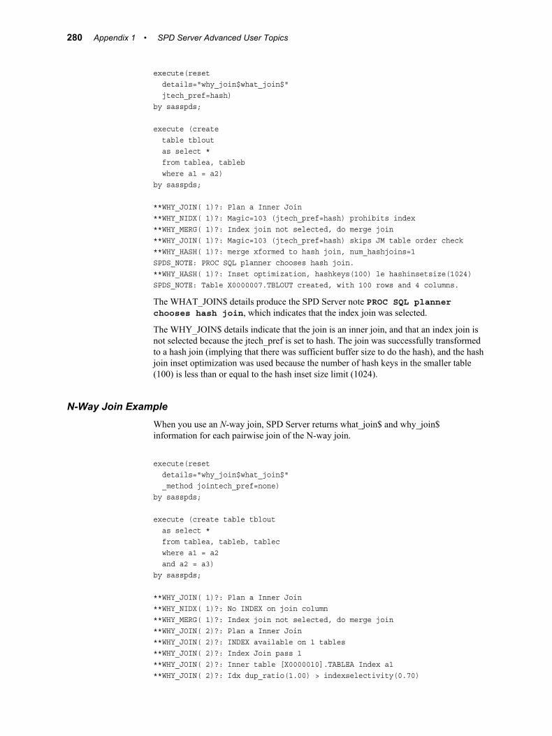
execute(reset details="why_join$what_join$" jtech_pref=hash) by sasspds;
execute (create table tblout as select * from tablea, tableb where a1 = a2) by sasspds;
**WHY_JOIN( 1)?: Plan a Inner Join **WHY_NIDX( 1)?: Magic=103 (jtech_pref=hash) prohibits index **WHY_MERG( 1)?: Index join not selected, do merge join **WHY_JOIN( 1)?: Magic=103 (jtech_pref=hash) skips JM table order check **WHY_HASH( 1)?: merge xformed to hash join, num_hashjoins=1 SPDS_NOTE: PROC SQL planner chooses hash join. **WHY_HASH( 1)?: Inset optimization, hashkeys(100) le hashinsetsize(1024) SPDS_NOTE: Table X0000007.TBLOUT created, with 100 rows and 4 columns.
The WHAT_JOIN$ details produce the SPD Server note PROC SQL planner chooses hash join, which indicates that the index join was selected.
The WHY_JOIN$ details indicate that the join is an inner join, and that an index join is not selected because the jtech_pref is set to hash. The join was successfully transformed to a hash join (implying that there was sufficient buffer size to do the hash), and the hash join inset optimization was used because the number of hash keys in the smaller table (100) is less than or equal to the hash inset size limit (1024).
N-Way Join ExampleWhen you use an N-way join, SPD Server returns what_join$ and why_join$ information for each pairwise join of the N-way join.
execute(reset details="why_join$what_join$" _method jointech_pref=none) by sasspds;
execute (create table tblout as select * from tablea, tableb, tablec where a1 = a2 and a2 = a3) by sasspds;
**WHY_JOIN( 1)?: Plan a Inner Join **WHY_NIDX( 1)?: No INDEX on join column **WHY_MERG( 1)?: Index join not selected, do merge join **WHY_JOIN( 2)?: Plan a Inner Join **WHY_JOIN( 2)?: INDEX available on 1 tables **WHY_JOIN( 2)?: Index Join pass 1 **WHY_JOIN( 2)?: Inner table [X0000010].TABLEA Index a1 **WHY_JOIN( 2)?: Idx dup_ratio(1.00) > indexselectivity(0.70)
280 Appendix 1 • SPD Server Advanced User Topics
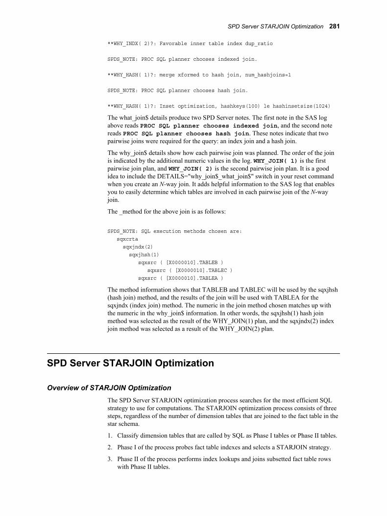
**WHY_INDX( 2)?: Favorable inner table index dup_ratio
SPDS_NOTE: PROC SQL planner chooses indexed join.
**WHY_HASH( 1)?: merge xformed to hash join, num_hashjoins=1
SPDS_NOTE: PROC SQL planner chooses hash join.
**WHY_HASH( 1)?: Inset optimization, hashkeys(100) le hashinsetsize(1024)
The what_join$ details produce two SPD Server notes. The first note in the SAS log above reads PROC SQL planner chooses indexed join, and the second note reads PROC SQL planner chooses hash join. These notes indicate that two pairwise joins were required for the query: an index join and a hash join.
The why_join$ details show how each pairwise join was planned. The order of the join is indicated by the additional numeric values in the log. WHY_JOIN( 1) is the first pairwise join plan, and WHY_JOIN( 2) is the second pairwise join plan. It is a good idea to include the DETAILS="why_join$_what_join$" switch in your reset command when you create an N-way join. It adds helpful information to the SAS log that enables you to easily determine which tables are involved in each pairwise join of the N-way join.
The _method for the above join is as follows:
SPDS_NOTE: SQL execution methods chosen are: sqxcrta sqxjndx(2) sqxjhsh(1) sqxsrc ( [X0000010].TABLEB ) sqxsrc ( [X0000010].TABLEC ) sqxsrc ( [X0000010].TABLEA )
The method information shows that TABLEB and TABLEC will be used by the sqxjhsh (hash join) method, and the results of the join will be used with TABLEA for the sqxjndx (index join) method. The numeric in the join method chosen matches up with the numeric in the why_join$ information. In other words, the sqxjhsh(1) hash join method was selected as the result of the WHY_JOIN(1) plan, and the sqxjndx(2) index join method was selected as a result of the WHY_JOIN(2) plan.
SPD Server STARJOIN Optimization
Overview of STARJOIN OptimizationThe SPD Server STARJOIN optimization process searches for the most efficient SQL strategy to use for computations. The STARJOIN optimization process consists of three steps, regardless of the number of dimension tables that are joined to the fact table in the star schema.
1. Classify dimension tables that are called by SQL as Phase I tables or Phase II tables.
2. Phase I of the process probes fact table indexes and selects a STARJOIN strategy.
3. Phase II of the process performs index lookups and joins subsetted fact table rows with Phase II tables.
SPD Server STARJOIN Optimization 281

Enabling STARJOIN Optimization in SPD ServerSPD Server STARJOIN optimization is enabled by default. For information about statement options that enable or disable the STARJOIN facility in SPD Server, see “STARJOIN RESET Statement Options” on page 93.
Classify Dimension Tables That Are Called by SQL as Phase I Tables or Phase II Tables
After the STARJOIN Planner validates the join subtree, join optimization begins. Join optimization is the process that searches for the most efficient SQL strategy to use to join the tables in the star schema.
The first step in SPD Server’s join optimization is to examine the dimension tables that were called by SQL for structures that SPD Server can use to improve performance. Each dimension table is classified as a Phase I table or a Phase II table. The structure of a dimension table and whether the SQL that you submit filters or subsets the table's contents determine its classification. SPD Server uses different processes to handle Phase I and Phase II dimension tables.
Phase I tables can improve performance. A Phase I table is a dimension table that is either very small (nine rows or fewer), or a dimension table whose SQL queries contain one or more filtering criteria that are expressed with a WHERE clause. A Phase II table is any dimension table that does not meet Phase I criteria. Rows in Phase II tables that are referenced in the SQL query are not subsetted.
Consider the star schema that is shown in Figure 7.1 on page 89, which contains the fact table Sales and the dimension tables Products, Supplier, Location, and Time.
Suppose that you submit an SQL query that requests transaction reports for all suppliers and for all products that meet the following criteria from the fact table Sales:
• the store location is North Carolina
• the time period is the month of January
The SQL query subsets the Location and Time tables, so SPD Server classifies the Location and Time tables as Phase I tables. The query requests information from all of the rows in the Product and Supplier tables. Because those tables are not subsetted by a WHERE clause in the SQL, STARJOIN classifies the Products and Supplier tables in this query as Phase II tables.
Now, using the same star schema, add more detail to the SQL query. Set up a new query that requests transaction reports from the fact table Sales for all stores where the location is the state of North Carolina, for the time period of the month of January, and for products where the supplier is from the state of North Carolina. The subsetted dimension tables Location, Time, and Supplier are classified as Phase I tables. The Products table, unfiltered by the SQL query, is classified as a Phase II table.
Dimension tables are classified as Phase I or Phase II tables because the two types of tables require different index probe methods.
Phase I Probes Fact Table Indexes and Selects a STARJOIN Strategy
Phase I uses the SQL join keys from the subsetted Phase I dimension tables to get a smaller set of candidate rows to query in the central fact table. After the Phase I index probe optimizes the candidate rows in the fact table, the probe examines index structures
282 Appendix 1 • SPD Server Advanced User Topics
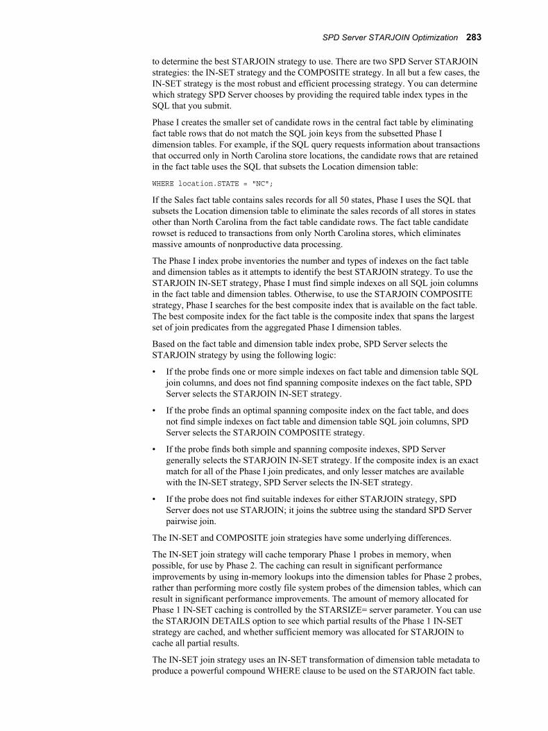
to determine the best STARJOIN strategy to use. There are two SPD Server STARJOIN strategies: the IN-SET strategy and the COMPOSITE strategy. In all but a few cases, the IN-SET strategy is the most robust and efficient processing strategy. You can determine which strategy SPD Server chooses by providing the required table index types in the SQL that you submit.
Phase I creates the smaller set of candidate rows in the central fact table by eliminating fact table rows that do not match the SQL join keys from the subsetted Phase I dimension tables. For example, if the SQL query requests information about transactions that occurred only in North Carolina store locations, the candidate rows that are retained in the fact table uses the SQL that subsets the Location dimension table:
WHERE location.STATE = "NC";
If the Sales fact table contains sales records for all 50 states, Phase I uses the SQL that subsets the Location dimension table to eliminate the sales records of all stores in states other than North Carolina from the fact table candidate rows. The fact table candidate rowset is reduced to transactions from only North Carolina stores, which eliminates massive amounts of nonproductive data processing.
The Phase I index probe inventories the number and types of indexes on the fact table and dimension tables as it attempts to identify the best STARJOIN strategy. To use the STARJOIN IN-SET strategy, Phase I must find simple indexes on all SQL join columns in the fact table and dimension tables. Otherwise, to use the STARJOIN COMPOSITE strategy, Phase I searches for the best composite index that is available on the fact table. The best composite index for the fact table is the composite index that spans the largest set of join predicates from the aggregated Phase I dimension tables.
Based on the fact table and dimension table index probe, SPD Server selects the STARJOIN strategy by using the following logic:
• If the probe finds one or more simple indexes on fact table and dimension table SQL join columns, and does not find spanning composite indexes on the fact table, SPD Server selects the STARJOIN IN-SET strategy.
• If the probe finds an optimal spanning composite index on the fact table, and does not find simple indexes on fact table and dimension table SQL join columns, SPD Server selects the STARJOIN COMPOSITE strategy.
• If the probe finds both simple and spanning composite indexes, SPD Server generally selects the STARJOIN IN-SET strategy. If the composite index is an exact match for all of the Phase I join predicates, and only lesser matches are available with the IN-SET strategy, SPD Server selects the IN-SET strategy.
• If the probe does not find suitable indexes for either STARJOIN strategy, SPD Server does not use STARJOIN; it joins the subtree using the standard SPD Server pairwise join.
The IN-SET and COMPOSITE join strategies have some underlying differences.
The IN-SET join strategy will cache temporary Phase 1 probes in memory, when possible, for use by Phase 2. The caching can result in significant performance improvements by using in-memory lookups into the dimension tables for Phase 2 probes, rather than performing more costly file system probes of the dimension tables, which can result in significant performance improvements. The amount of memory allocated for Phase 1 IN-SET caching is controlled by the STARSIZE= server parameter. You can use the STARJOIN DETAILS option to see which partial results of the Phase 1 IN-SET strategy are cached, and whether sufficient memory was allocated for STARJOIN to cache all partial results.
The IN-SET join strategy uses an IN-SET transformation of dimension table metadata to produce a powerful compound WHERE clause to be used on the STARJOIN fact table.
SPD Server STARJOIN Optimization 283
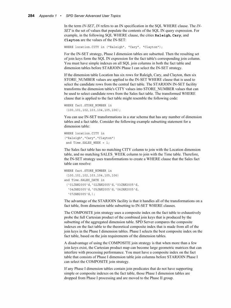
In the term IN-SET, IN refers to an IN specification in the SQL WHERE clause. The IN-SET is the set of values that populate the contents of the SQL IN query expression. For example, in the following SQL WHERE clause, the cities Raleigh, Cary, and Clayton are the values of the IN-SET:
WHERE location.CITY in ("Raleigh", "Cary", "Clayton");
For the IN-SET strategy, Phase I dimension tables are subsetted. Then the resulting set of join keys form the SQL IN expression for the fact table's corresponding join column. You must have simple indexes on all SQL join columns in both the fact table and dimension tables before STARJOIN Phase I can select the IN-SET strategy.
If the dimension table Location has six rows for Raleigh, Cary, and Clayton, then six STORE_NUMBER values are applied to the IN-SET WHERE clause that is used to select the candidate rows from the central fact table. The STARJOIN IN-SET facility transforms the dimension table's CITY values into STORE_NUMBER values that can be used to select candidate rows from the Sales fact table. The transformed WHERE clause that is applied to the fact table might resemble the following code:
WHERE fact.STORE_NUMBER in (100,101,102,103,104,105,106);
You can use IN-SET transformations in a star schema that has any number of dimension tables and a fact table. Consider the following example subsetting statement for a dimension table:
WHERE location.CITY in("Raleigh","Cary","Clayton") and Time.SALES_WEEK = 1;
The Sales fact table has no matching CITY column to join with the Location dimension table, and no matching SALES_WEEK column to join with the Time table. Therefore, the IN-SET strategy uses transformations to create a WHERE clause that the Sales fact table can resolve:
WHERE fact.STORE_NUMBER in (100,101,102,103,104,105,106)and Time.SALES_DATE in ('01JAN2005'd,'02JAN2005'd,'03JAN2005'd, '04JAN2005'd,'05JAN2005'd,'06JAN2005'd, '07JAN2005'd,);
The advantage of the STARJOIN facility is that it handles all of the transformations on a fact table, from dimension table subsetting to IN-SET WHERE clauses.
The COMPOSITE join strategy uses a composite index on the fact table to exhaustively probe the full Cartesian product of the combined join keys that is produced by the subsetting of the aggregated dimension table. SPD Server compares the composite indexes on the fact table to the theoretical composite index that is made from all of the join keys in the Phase I dimension tables. Phase I selects the best composite index on the fact table, based on the join requirements of the dimension tables.
A disadvantage of using the COMPOSITE join strategy is that when more than a few join keys exist, the Cartesian product map can become large geometric matrices that can interfere with processing performance. You must have a composite index on the fact table that consists of Phase I dimension table join columns before STARJOIN Phase I can select the COMPOSITE join strategy.
If any Phase I dimension tables contain join predicates that do not have supporting simple or composite indexes on the fact table, those Phase I dimension tables are dropped from Phase I processing and are moved to the Phase II group.
284 Appendix 1 • SPD Server Advanced User Topics

Phase II Performs Index Lookups and Joins Subsetted Fact Table Rows with Phase II Tables
Phase I optimizes the join strategies between the Phase I dimension tables and the candidate rows from the fact table . After Phase I terminates, Phase II takes over. Phase II completes the indicated joins between the candidate rows from the fact table and the corresponding rows in the subsetted Phase I dimension tables. After Phase II completes the joins with the Phase I dimension tables, Phase II performs index lookups from the fact table to the Phase dimension II tables. Phase II dimension tables should have indexes created on all columns that join with the fact table.
When SPD Server completes the STARJOIN Phase I and Phase II tasks, the STARJOIN optimizations have been performed, the STARJOIN strategy has been selected, and the subsetted dimension tables and fact table joins are ready to run and produce the SQL results set that you want.
SPD Server STARJOIN Optimization 285

286 Appendix 1 • SPD Server Advanced User Topics

Appendix 2
SAS Scalable Performance Data (SPD) Server Frequently Asked Questions
Does SPD Server support files that are larger than 2 Gigabytes in size?
Yes. SPD Server does so by breaking up larger files into partitions that are smaller than 2 Gigabytes. The SPD Server host performs this function automatically and it requires no special syntax.
Can I create file systems that are larger than 2 Gigabytes in size?Yes, if you use a volume manager that lets you create file systems greater than 2 Gigabytes. SAS recommends this practice.
How do SPD Server client and server processes communicate?An SPD Server client communicates with three SPD Server processes.
When a client issues a LIBNAME assignment to the SPD Server host, the client communicates with the SPD Server Name Server process using the HOST= and SERV= options that were specified in the LIBNAME connection. The HOST= option specifies the host system where the SPD Server Name Server is running, and the SERV= option is the well-known port number of the SPD Server Name Server that was specified when the software was started. The SPD Server Name Server ensures that the domain of the LIBNAME assignment is valid and returns the HOST= and SERV= option settings to the client. This ends the interaction of the client with the SPD Server Name Server for that LIBNAME assignment. The client communicates with the SPDSSERV process to complete the LIBNAME assignment.
The SPDSSERV process authenticates the USER and PASSWORD portion of the LIBNAME assignment, and validates whether the USER has access to the domain. If the LIBNAME is successfully authenticated, the SPDSSERV process forks and executes a user proxy, the SPDSBASE process, which continues to service all other client requests for that LIBNAME connection. Subsequent LIBNAME assignments from the same client that are resolved to the same SPD Server user and SPDSSERV context are passed directly to SPDSBASE for processing without any further SPDSSERV interaction. (No further interaction is required because the authentication is inherited by subsequent LIBNAME assignments.)
LIBNAME assignments from the same client for a different SPD Server user or LIBNAME assignments to a domain that is serviced by a different SPDSSERV results in a new SPDSBASE process to service that LIBNAME assignment.
Connections that use the record-level locking option LOCKING=YES to connect to a server in any domain are handled differently. All LIBNAME assignments share the same
287
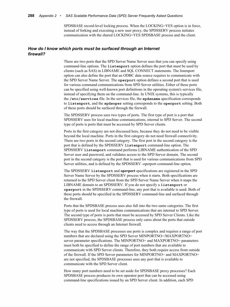
SPDSBASE record-level locking process. When the LOCKING=YES option is in force, instead of forking and executing a new user proxy, the SPDSSERV process initiates communication with the shared LOCKING=YES SPDSBASE process and the client.
How do I know which ports must be surfaced through an Internet firewall?
There are two ports that the SPD Server Name Server uses that you can specify using command-line options. The listenport option defines the port that must be used by clients (such as SAS) in LIBNAME and SQL CONNECT statements. The listenport option can also define the port that an ODBC data source requires to communicate with the SPD Server Name Server. The operport option defines a second port that is used for various command communications from SPD Server utilities. Either of these ports can be specified using well-known port definitions in the operating system's services file, instead of specifying them on the command-line. In UNIX systems, this is typically the /etc/services file. In the services file, the spdsname specification corresponds to listenport, and the spdsoper setting corresponds to the operport setting. Both of these ports should be surfaced through the firewall.
The SPDSSERV process uses two types of ports. The first type of port is a port that SPDSSERV uses for local machine communications, internal to SPD Server. The second type of ports is ports that must be accessed by SPD Server clients.
Ports in the first category are not discussed here, because they do not need to be visible beyond the local machine. Ports in the first category do not need firewall connectivity. There are two ports in the second category. The first port in the second category is the port that is defined by the SPDSSERV listenport command-line option. The SPDSSERV listenport command performs LIBNAME authentication of the SPD Server user and password, and validates access to the SPD Server domain. The second port in the second category is the port that is used for various communications from SPD Server utilities, and is defined by the SPDSSERV -operport command-line option.
The SPDSSERV listenport and operport specifications are registered in the SPD Server Name Server by the SPDSSERV process when it starts. Both specifications are returned to the SPD Server client from the SPD Server Name Server when it maps the LIBNAME domain to an SPDSSERV. If you do not specify a listenport or operport in the SPDSSERV command-line, any port that is available is used. Both of these ports should be specified in the SPDSSERV command-line and surfaced through the firewall.
Ports that the SPDSBASE process uses also fall into the two same categories. The first type of ports is used for local machine communications that are internal to SPD Server. The second type of ports is ports that must be accessed by SPD Server Clients. Like the SPDSSERV process, the SPDSBASE process only cares about the ports that outside clients need to access through an Internet firewall.
The way that the SPDSBASE processes use ports is complex and requires a range of port numbers that are declared using the SPD Server MINPORTNO=/MAXPORTNO= server parameter specifications. The MINPORTNO= and MAXPORTNO= parameters must both be specified to define the range of port numbers that are available to communicate with SPD Server clients. Therefore, they both require access from outside of the firewall. If the SPD Server parameters for MINPORTNO= and MAXPORTNO= are not specified, the SPDSBASE processes uses any port that is available to communicate with the SPD Server client.
How many port numbers need to be set aside for SPDSBASE proxy processes? Each SPDSBASE process produces its own operator port that can be accessed using command-line specifications issued by an SPD Server client. In addition, each SPD
288 Appendix 2 • SAS Scalable Performance Data (SPD) Server Frequently Asked Questions

Server table that is opened creates its own port. Each table's port becomes a dedicated data transfer connection that is used to stream data transfers to and from the SPD Server client. SPD Server table ports are normally dynamically assigned, unless the MINPORTNO= and MAXPORTNO= parameters have been specified. If the MINPORTNO= and MAXPORTNO= parameters have been specified, SPD Server table ports are assigned from within the specified port range.
Therefore, it follows that the range of ports that is specified for the MINPORTNO= and MAXPORTNO= parameters must consider the peak number of concurrent LIBNAME connections that are made to the server, as well as the I/O streams that are channeled between the SPDSBASE processes and the SPD Server clients.
The following ports must be surfaced for access beyond the firewall:
• Two SPD Server Name Server ports, listenport and operport , must be surfaced for access beyond the firewall. This is also true for any other ports that are identified in SPDSNAME and SPDSOPER services.
• Two SPDSSERV ports: listenport and operport , as well as any other ports that are identified in SPDSSERV_SAS and SPDSSERV_OPER services.
• Any other ports that are defined in the MINPORTNO= and MAXPORTNO= range that is specified in the spdsserv.parm file.
How does SPD Server interact with multi-homed hosts?A multi-homed host is a machine that has two or more IP addresses. For SPD Server to work properly on host machines that have more than one IP address, you must define which IP address you want to associate with the socket bind calls. Socket bind calls listen for the SPD Server Name Server and the SPDSSERV processes. You use the SPDSBINDADDR environment variable to define the preferred IP address. You set the SPDSBINDADDR environment variable in the rc.spds script that you use to initiate the SPD Server Name Server and SPDSSERV processes on the SPD Server host machine.
Can I use standard UNIX backup procedures?Yes. SPD Server files are standard files. If all the components of a table are in the same directory, then you can use the standard backup utility. This is our recommendation. SPD Server includes an incremental backup utility.
What do I need to know about SPD Server installation? How long does it take?
The SPD Server install is quick and easy to do. The hard-copy installation instructions and shell scripts that are included on the installation media guides you through the installation process. Installation and verification take less than an hour. You might need additional time if you have several SAS client platforms to update.
On UNIX, the SPD Server installation can be performed using a non-privileged UNIX account, although to implement all recommendations, UNIX root privilege is required.
Is it necessary to run UNIX SPD Server as root?No. SAS recommends that you use a UNIX user ID other than root to run your production SPD Server environment. Root access is not required to run the SPD Server environment when you properly configure the UNIX directory ownership and
SAS Scalable Performance Data (SPD) Server Frequently Asked Questions 289
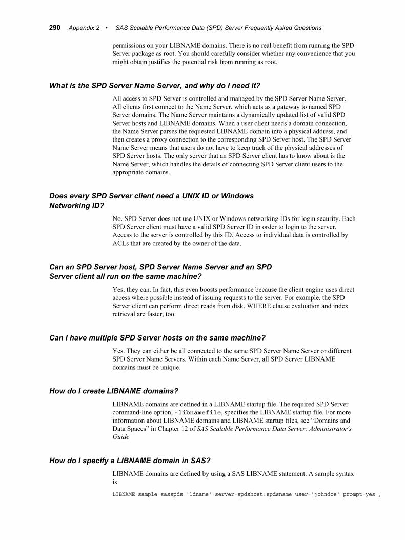
permissions on your LIBNAME domains. There is no real benefit from running the SPD Server package as root. You should carefully consider whether any convenience that you might obtain justifies the potential risk from running as root.
What is the SPD Server Name Server, and why do I need it?All access to SPD Server is controlled and managed by the SPD Server Name Server. All clients first connect to the Name Server, which acts as a gateway to named SPD Server domains. The Name Server maintains a dynamically updated list of valid SPD Server hosts and LIBNAME domains. When a user client needs a domain connection, the Name Server parses the requested LIBNAME domain into a physical address, and then creates a proxy connection to the corresponding SPD Server host. The SPD Server Name Server means that users do not have to keep track of the physical addresses of SPD Server hosts. The only server that an SPD Server client has to know about is the Name Server, which handles the details of connecting SPD Server client users to the appropriate domains.
Does every SPD Server client need a UNIX ID or Windows Networking ID?
No. SPD Server does not use UNIX or Windows networking IDs for login security. Each SPD Server client must have a valid SPD Server ID in order to login to the server. Access to the server is controlled by this ID. Access to individual data is controlled by ACLs that are created by the owner of the data.
Can an SPD Server host, SPD Server Name Server and an SPD Server client all run on the same machine?
Yes, they can. In fact, this even boosts performance because the client engine uses direct access where possible instead of issuing requests to the server. For example, the SPD Server client can perform direct reads from disk. WHERE clause evaluation and index retrieval are faster, too.
Can I have multiple SPD Server hosts on the same machine?Yes. They can either be all connected to the same SPD Server Name Server or different SPD Server Name Servers. Within each Name Server, all SPD Server LIBNAME domains must be unique.
How do I create LIBNAME domains?LIBNAME domains are defined in a LIBNAME startup file. The required SPD Server command-line option, -libnamefile, specifies the LIBNAME startup file. For more information about LIBNAME domains and LIBNAME startup files, see “Domains and Data Spaces” in Chapter 12 of SAS Scalable Performance Data Server: Administrator's Guide
How do I specify a LIBNAME domain in SAS?LIBNAME domains are defined by using a SAS LIBNAME statement. A sample syntax is
LIBNAME sample sasspds 'ldname' server=spdshost.spdsname user='johndoe' prompt=yes ;
290 Appendix 2 • SAS Scalable Performance Data (SPD) Server Frequently Asked Questions

where
sample is the name of the libref
sasspds is the name of the SPD Server engine
ldname is the LIBNAME domain
spdshost is the IP name of the node that is running the Name Server
spdsname is the port number that the Name Server uses
johndoe is the SPD Server login ID
prompt is the prompt for password Y | N
Is there anything else I have to change to run my existing SAS applications?
Typically, no. Once the librefs have been assigned, your existing SAS application runs unchanged.
How can I get existing data loaded into an SPD Server table?There are several ways to accomplish this. Here are the three most common:
1. Use PROC COPY:
PROC COPY in=old out=spds memtype=data ; run ;
This copies the data and build any existing indexes automatically.
2. Use the DATA Step and SET statement:
DATA spds.a ; set old.a ; run ;
This copies the data. You have to specify the indexes that you want to build.
DATA spds.a(index=(z)); set old.a ; run ;
This copies the data and create an index on variable Z.
3. Use the Microsoft Windows ODBC driver.
Also, see “Migrating Tables between SAS and SPD Server” on page 22, which examines table conversions.
Can SPD Server create indexes in parallel?Yes, SPD Server can create multiple indexes at the same time. It does this by launching one thread per index and driving them all at the same time. You can accomplish this with
SAS Scalable Performance Data (SPD) Server Frequently Asked Questions 291

PROC DATASETS lib=spds ; modify a(asyncindex=yes) ; index create x ; index create y ; index create comp=(x y) ;quit;
In the above example, X, Y, and COMP are created in parallel. Notice the ASYNCINDEX=YES data set option in the MODIFY statement.
%LET spdsiasy=YES ;PROC DATASETS lib=spds ; modify a ; index create x ; index create y ; modify a ; index create comp=(x y) comp2=(y x) ;quit ;
In the above example, X and Y are created in parallel; COMP and COMP2 are created in a second parallel index create as soon as the first pair completes. Notice the use of the SPDSIASY macro variable to specify parallel index creation. In this example, a table scan is required for each batch of indexes identified for creation in parallel: one table scan for the X and Y indexes and a second table scan for the COMP and COMP2 indexes.
How many indexes should you create in parallel? It depends on how many CPUs are in the SMP configuration, available disk space for index key sorting, and other tasks. Some results show that on an 8-way UltraSparc, you can create four indexes in almost the same time it takes to create 1. You can group index creates to minimize table scans or auxiliary disk space consumption, but generally there is an inverse relationship between the two: minimizing table scans requires more auxiliary disk space and vice versa. The Help documentation contains more information about “Parallel Index Creation” on page 127.
Does SPD Server append indexes in parallel?Yes, SPD Server appends indexes in parallel by default.
What are ACLs and how do I use them to control access to data tables?
ACLs define who can access a data table and what type of access they are granted. Currently, there are four levels of access defined: Access List Entry, Owner Access, Group Access, and Universal Access. Every SPD Server user has access to at least one group. During login, an SPD Server user must specify a particular ACL group if the SPD Server password file has the user entered as a member of more than one group. Every data table has an ACL owner and the owner's ACL group attached to it. The precedence of the access levels is the following:
• Access List Entry
• Owner Access
292 Appendix 2 • SAS Scalable Performance Data (SPD) Server Frequently Asked Questions

• Group Access
• Universal Access
Types of access are Read, Write, Alter, and Control. To create access lists that you must have CONTROL access. The owner by default has control access. For more information about ACL access lists and commands, see “Using the ACL Command Set” in Chapter 14 of SAS Scalable Performance Data Server: Administrator's Guide.
How do I get a list of the SAS macro variables introduced for SPD Server?
In a SAS session, get into PROC SPDO and issue the SPDSMAC command. For example:
LIBNAME foo sasspds ... ; PROC SPDO lib=foo ; SPDSMAC ;
For more information, see “SAS Scalable Performance Data (SPD) Server Macro Variables ” on page 152.
What about unique indexes? Can I do something to speed appends?
You can use the SPDSAUNQ=YES server option to speed up appends to unique indexes. For information about the SPDSAUNQ option, see “SPDSAUNQ=” on page 171.
What about disk compression for SPD Server tables?You can request compression for an SPD Server table by using the COMPRESS= data set option. You can also set a macro variable named SPDSDCMP to the same value that you would set in the COMPRESS= option. This causes compression on all data sets you generate without explicitly specifying COMPRESS= on each DATA step. SPD Server compresses your table set by "blocks" and the way you control this amount is through the IOBLOCKSIZE= table option. Once you create a compressed table, the compression block size (that is, the number observations per block) cannot be changed. You must PROC COPY the data set to a new data set with a different IOBLOCKSIZE= on the output data set.
For more information about SPD Server disk compression settings, see “COMPRESS=” on page 196.
In any case, you select the default SPD Server compression by asserting COMPRESS=YES or using %let SPDSDCMP=YES. The default compression algorithm is a run-length compression.
What about estimates for disk space consumption when using SPD Server?
Overview of Disk Space ConsumptionThe answer to this question depends on what type of component file within the SPD Server data you need to estimate. Recall that there are three classes of component files
SAS Scalable Performance Data (SPD) Server Frequently Asked Questions 293

that make up an SPD Server table: metadata, data, and indexes. You always get the first two for every table. You get an index component file for each index that you create on the table.
Metadata Space ConsumptionThe approximate estimate here is:
SpaceBytes = 12Kb + (#columns * 120) + (5Kb * #indexes)
This estimate increases if you delete observations from the table or use compression on the table. In general, the size of this component file should not exceed approximately 400K.
Data Space ConsumptionThe estimate here is for uncompressed tables:
SpaceBytes = #rows * RowLength
Your space consumption for compressed tables obviously varies with the compression factor for your table as a whole.
Hybrid Index Space ConsumptionThe hybrid index uses two data files. The .hbx file contains the global portion of the hybrid index. You can estimate space consumption approximately for the .hbx component of a hybrid index as follows:
If the index is NOT unique:
number_of_discrete_values_in_the_index * (22.5 + (length_of_columns_composing_the_index))
If the index IS unique:
number_of_discrete_value_in_the_index * (6 + (length_of_columns_composing_the_index))
The .idx file contains the per-value segment lists and bitmap portion of the hybrid index. Estimating disk space consumption for this file is much more difficult than the .hbx file. This is because the .idx file size depends on the distribution of the key values across the rows of the table. The size also depends on the number of updates and appends performed on the index. The .idx files of an indexed table initially created with "n" rows consumes considerably less space than the .idx files of an identical table created and with several append or updates performed afterward. The wasted space in the latter example can be reclaimed by reorganizing the index.
With the above in mind, a worst case estimate for space consumption of the .idx component of a hybrid index is:
8192 + (number_of_discrete_values_in_more_than_one_obs * (24 + (avg_number_of_segments_per_value * (16 + (seg_size / 8)))))
This estimate does not consider the compression factor for the bitmaps, which could be substantial. The fewer occurrences of a value in a given segment, the more the bitmap for that segment can be compressed. The uncompressed bitmap size is the (seg_size/8) component of the algorithm.
294 Appendix 2 • SAS Scalable Performance Data (SPD) Server Frequently Asked Questions
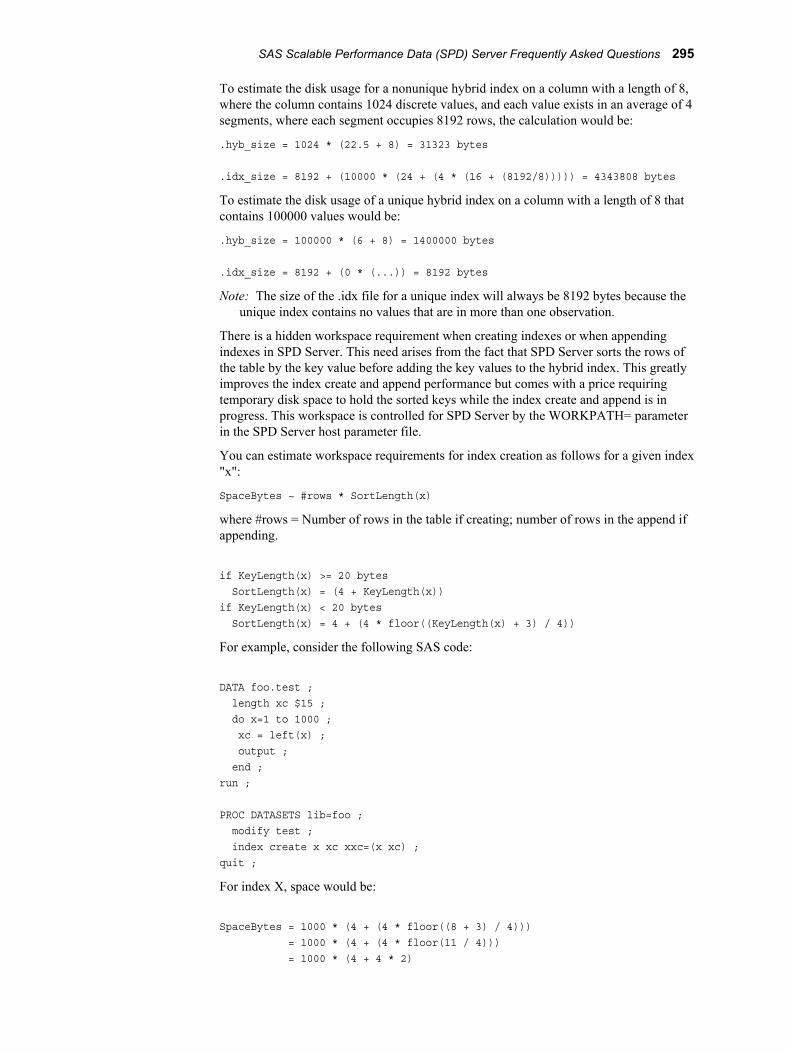
To estimate the disk usage for a nonunique hybrid index on a column with a length of 8, where the column contains 1024 discrete values, and each value exists in an average of 4 segments, where each segment occupies 8192 rows, the calculation would be:
.hyb_size = 1024 * (22.5 + 8) = 31323 bytes
.idx_size = 8192 + (10000 * (24 + (4 * (16 + (8192/8))))) = 4343808 bytes
To estimate the disk usage of a unique hybrid index on a column with a length of 8 that contains 100000 values would be:
.hyb_size = 100000 * (6 + 8) = 1400000 bytes
.idx_size = 8192 + (0 * (...)) = 8192 bytes
Note: The size of the .idx file for a unique index will always be 8192 bytes because the unique index contains no values that are in more than one observation.
There is a hidden workspace requirement when creating indexes or when appending indexes in SPD Server. This need arises from the fact that SPD Server sorts the rows of the table by the key value before adding the key values to the hybrid index. This greatly improves the index create and append performance but comes with a price requiring temporary disk space to hold the sorted keys while the index create and append is in progress. This workspace is controlled for SPD Server by the WORKPATH= parameter in the SPD Server host parameter file.
You can estimate workspace requirements for index creation as follows for a given index "x":
SpaceBytes ~ #rows * SortLength(x)
where #rows = Number of rows in the table if creating; number of rows in the append if appending.
if KeyLength(x) >= 20 bytes SortLength(x) = (4 + KeyLength(x))if KeyLength(x) < 20 bytes SortLength(x) = 4 + (4 * floor((KeyLength(x) + 3) / 4))
For example, consider the following SAS code:
DATA foo.test ; length xc $15 ; do x=1 to 1000 ; xc = left(x) ; output ; end ;run ;
PROC DATASETS lib=foo ; modify test ; index create x xc xxc=(x xc) ;quit ;
For index X, space would be:
SpaceBytes = 1000 * (4 + (4 * floor((8 + 3) / 4))) = 1000 * (4 + (4 * floor(11 / 4))) = 1000 * (4 + 4 * 2)
SAS Scalable Performance Data (SPD) Server Frequently Asked Questions 295

= 12,000
For index XC, space would be:
SpaceBytes = 1000 * (4 + (4 * floor(15 + 3) / 4))) = 1000 * (4 + (4 * floor(18 / 4))) = 1000 * (4 + 4 * 4) = 20,000
For index XXC, space would be:
SpaceBytes = 1000 * (4 + 23) = 1000 * 27 = 27,000
There is one other factor that plays into workspace computation: Are you creating the indexes in parallel or serially? If you create the indexes in parallel by using the ASYNCINDEX=YES data set option or by asserting the SPDSIASY macro variable, you need to sum the space requirements for each index that you create in the same create phase.
As is noted in the FAQ example about creating SPD Server indexes in parallel, “Can SPD Server create indexes in parallel?” on page 291, the indexes X and Y constitute a create phase, as do COMP and COMP2. You would need to sum the space requirement for X and Y, and for COMP and COMP2, and take the maximum of these two numbers to get the workspace needed to complete the PROC DATASETS indexes successfully.
The same applies to PROC APPEND runs when appending to the table with indexes. In this case all of the indexes are appended in parallel, so you would need to sum the workspace requirement across all indexes.
How can I estimate the transient space needed to perform PROC SORT / BY processing?
Workspace is required for SPD Server sorting just as it is required for SPD Server sorted index creation. There are two modes of sorting in SPD Server: tag and non-tag sorting. In either case, you sort based on the columns selected in the BY clause. The difference is in the auxiliary data that is carried along by the sort in addition to the key constructed from the BY columns. The default for SPD Server is to use the non-tag sort.
In the case of non-tag sorting, SPD Server carries along the entire row contents (that is, all columns) as the auxiliary data for the key. In the mode of tag sorting, SPD Server only carries along the row ID that points back to the original table row as the auxiliary data. You control the amount of a sort problem that fits in memory at one time by the SPD Server parameter SORTSIZE. Obviously, for a given sort size the number of sort records that fits is a function of the sort mode(#records = SORTSIZE / (SortKeyLength + AuxillaryLength)). When the sort problem does not fit in one SORTSIZE bin, the bins are written to workspace on disk and then merged back to make the final sorted run.
Estimating the disk space required for SPD Server sorting depends on the mode.
For non-tag sorting the estimate is
SpaceBytes = #rows * (SortKeyLength + 4 + RowLength)
For tag sorting the estimate is
SpaceBytes = #rows * (SortKeyLength + 8)
296 Appendix 2 • SAS Scalable Performance Data (SPD) Server Frequently Asked Questions
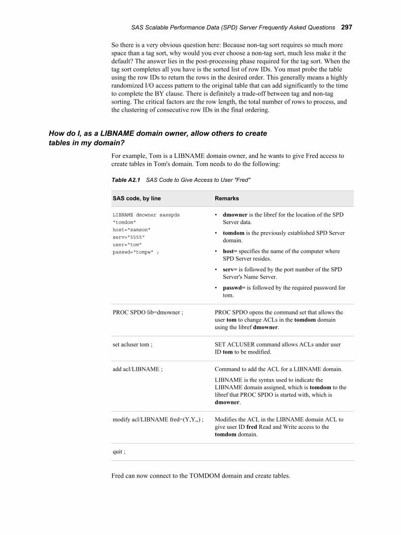
So there is a very obvious question here: Because non-tag sort requires so much more space than a tag sort, why would you ever choose a non-tag sort, much less make it the default? The answer lies in the post-processing phase required for the tag sort. When the tag sort completes all you have is the sorted list of row IDs. You must probe the table using the row IDs to return the rows in the desired order. This generally means a highly randomized I/O access pattern to the original table that can add significantly to the time to complete the BY clause. There is definitely a trade-off between tag and non-tag sorting. The critical factors are the row length, the total number of rows to process, and the clustering of consecutive row IDs in the final ordering.
How do I, as a LIBNAME domain owner, allow others to create tables in my domain?
For example, Tom is a LIBNAME domain owner, and he wants to give Fred access to create tables in Tom's domain. Tom needs to do the following:
Table A2.1 SAS Code to Give Access to User "Fred"
SAS code, by line Remarks
LIBNAME dmowner sasspds"tomdom"host="samson"serv="5555"user="tom"passwd="tompw" ;
• dmowner is the libref for the location of the SPD Server data.
• tomdom is the previously established SPD Server domain.
• host= specifies the name of the computer where SPD Server resides.
• serv= is followed by the port number of the SPD Server's Name Server.
• passwd= is followed by the required password for tom.
PROC SPDO lib=dmowner ; PROC SPDO opens the command set that allows the user tom to change ACLs in the tomdom domain using the libref dmowner.
set acluser tom ; SET ACLUSER command allows ACLs under user ID tom to be modified.
add acl/LIBNAME ; Command to add the ACL for a LIBNAME domain.
LIBNAME is the syntax used to indicate the LIBNAME domain assigned, which is tomdom to the libref that PROC SPDO is started with, which is dmowner.
modify acl/LIBNAME fred=(Y,Y,,) ; Modifies the ACL in the LIBNAME domain ACL to give user ID fred Read and Write access to the tomdom domain.
quit ;
Fred can now connect to the TOMDOM domain and create tables.
SAS Scalable Performance Data (SPD) Server Frequently Asked Questions 297
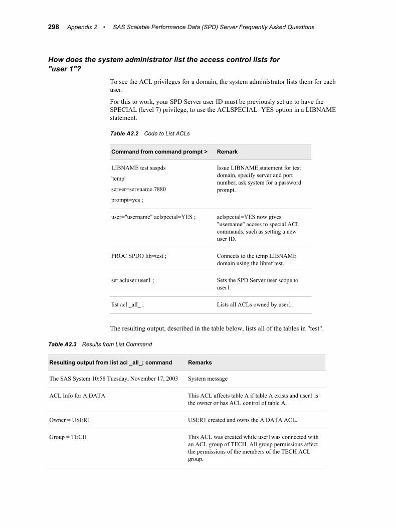
How does the system administrator list the access control lists for "user 1"?
To see the ACL privileges for a domain, the system administrator lists them for each user.
For this to work, your SPD Server user ID must be previously set up to have the SPECIAL (level 7) privilege, to use the ACLSPECIAL=YES option in a LIBNAME statement.
Table A2.2 Code to List ACLs
Command from command prompt > Remark
LIBNAME test saspds
'temp'
server=servname.7880
prompt=yes ;
Issue LIBNAME statement for test domain, specify server and port number, ask system for a password prompt.
user="username" aclspecial=YES ; aclspecial=YES now gives "username" access to special ACL commands, such as setting a new user ID.
PROC SPDO lib=test ; Connects to the temp LIBNAME domain using the libref test.
set acluser user1 ; Sets the SPD Server user scope to user1.
list acl _all_ ; Lists all ACLs owned by user1.
The resulting output, described in the table below, lists all of the tables in "test".
Table A2.3 Results from List Command
Resulting output from list acl _all_; command Remarks
The SAS System 10:58 Tuesday, November 17, 2003 System message
ACL Info for A.DATA This ACL affects table A if table A exists and user1 is the owner or has ACL control of table A.
Owner = USER1 USER1 created and owns the A.DATA ACL.
Group = TECH This ACL was created while user1was connected with an ACL group of TECH. All group permissions affect the permissions of the members of the TECH ACL group.
298 Appendix 2 • SAS Scalable Performance Data (SPD) Server Frequently Asked Questions
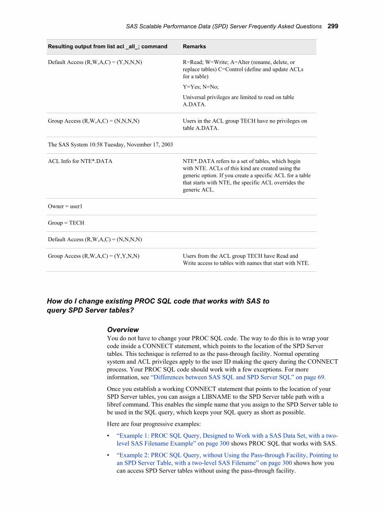
Resulting output from list acl _all_; command Remarks
Default Access (R,W,A,C) = (Y,N,N,N) R=Read; W=Write; A=Alter (rename, delete, or replace tables) C=Control (define and update ACLs for a table)
Y=Yes; N=No;
Universal privileges are limited to read on table A.DATA.
Group Access (R,W,A,C) = (N,N,N,N) Users in the ACL group TECH have no privileges on table A.DATA.
The SAS System 10:58 Tuesday, November 17, 2003
ACL Info for NTE*.DATA NTE*.DATA refers to a set of tables, which begin with NTE. ACLs of this kind are created using the generic option. If you create a specific ACL for a table that starts with NTE, the specific ACL overrides the generic ACL.
Owner = user1
Group = TECH
Default Access (R,W,A,C) = (N,N,N,N)
Group Access (R,W,A,C) = (Y,Y,N,N) Users from the ACL group TECH have Read and Write access to tables with names that start with NTE.
How do I change existing PROC SQL code that works with SAS to query SPD Server tables?
OverviewYou do not have to change your PROC SQL code. The way to do this is to wrap your code inside a CONNECT statement, which points to the location of the SPD Server tables. This technique is referred to as the pass-through facility. Normal operating system and ACL privileges apply to the user ID making the query during the CONNECT process. Your PROC SQL code should work with a few exceptions. For more information, see “Differences between SAS SQL and SPD Server SQL” on page 69.
Once you establish a working CONNECT statement that points to the location of your SPD Server tables, you can assign a LIBNAME to the SPD Server table path with a libref command. This enables the simple name that you assign to the SPD Server table to be used in the SQL query, which keeps your SQL query as short as possible.
Here are four progressive examples:
• “Example 1: PROC SQL Query, Designed to Work with a SAS Data Set, with a two-level SAS Filename Example” on page 300 shows PROC SQL that works with SAS.
• “Example 2: PROC SQL Query, without Using the Pass-through Facility, Pointing to an SPD Server Table, with a two-level SAS Filename” on page 300 shows how you can access SPD Server tables without using the pass-through facility.
SAS Scalable Performance Data (SPD) Server Frequently Asked Questions 299
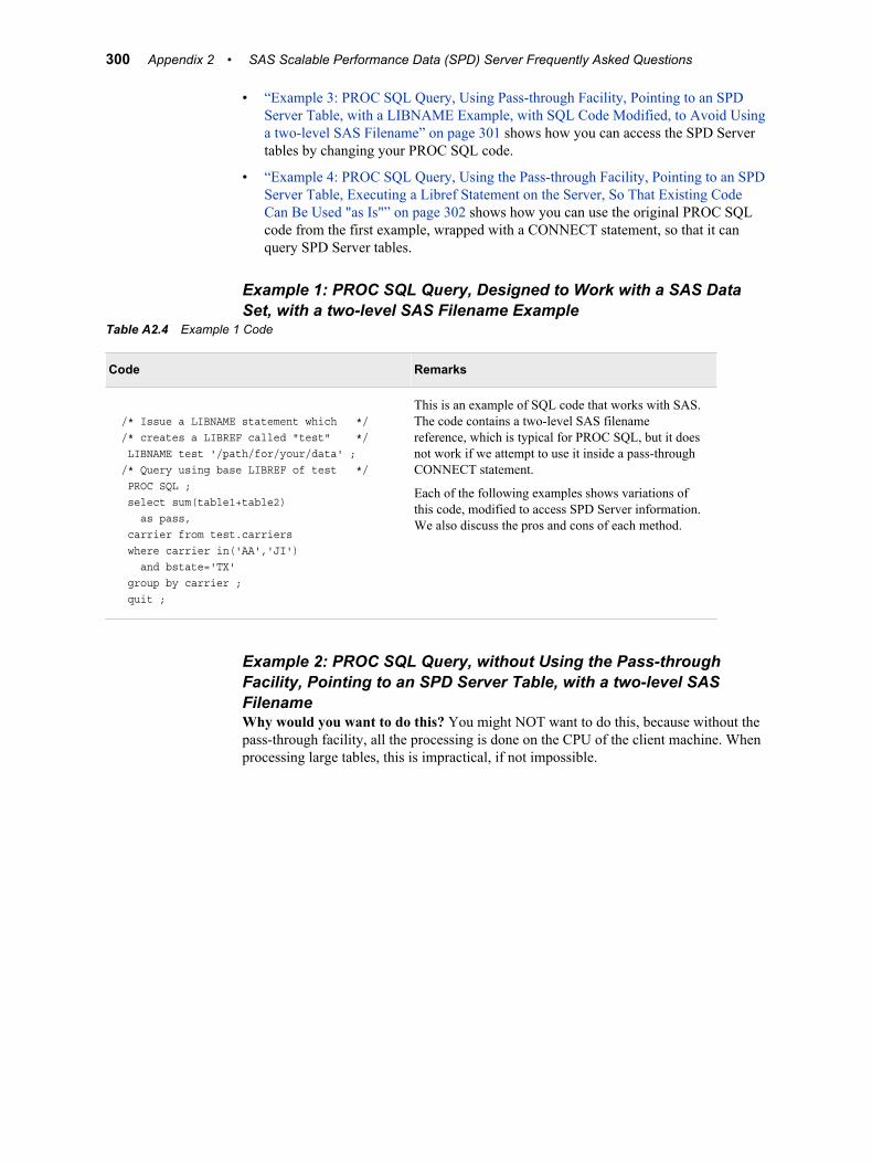
• “Example 3: PROC SQL Query, Using Pass-through Facility, Pointing to an SPD Server Table, with a LIBNAME Example, with SQL Code Modified, to Avoid Using a two-level SAS Filename” on page 301 shows how you can access the SPD Server tables by changing your PROC SQL code.
• “Example 4: PROC SQL Query, Using the Pass-through Facility, Pointing to an SPD Server Table, Executing a Libref Statement on the Server, So That Existing Code Can Be Used "as Is"” on page 302 shows how you can use the original PROC SQL code from the first example, wrapped with a CONNECT statement, so that it can query SPD Server tables.
Example 1: PROC SQL Query, Designed to Work with a SAS Data Set, with a two-level SAS Filename Example
Table A2.4 Example 1 Code
Code Remarks
/* Issue a LIBNAME statement which */ /* creates a LIBREF called "test" */ LIBNAME test '/path/for/your/data' ; /* Query using base LIBREF of test */ PROC SQL ; select sum(table1+table2) as pass, carrier from test.carriers where carrier in('AA','JI') and bstate='TX' group by carrier ; quit ;
This is an example of SQL code that works with SAS. The code contains a two-level SAS filename reference, which is typical for PROC SQL, but it does not work if we attempt to use it inside a pass-through CONNECT statement.
Each of the following examples shows variations of this code, modified to access SPD Server information. We also discuss the pros and cons of each method.
Example 2: PROC SQL Query, without Using the Pass-through Facility, Pointing to an SPD Server Table, with a two-level SAS FilenameWhy would you want to do this? You might NOT want to do this, because without the pass-through facility, all the processing is done on the CPU of the client machine. When processing large tables, this is impractical, if not impossible.
300 Appendix 2 • SAS Scalable Performance Data (SPD) Server Frequently Asked Questions
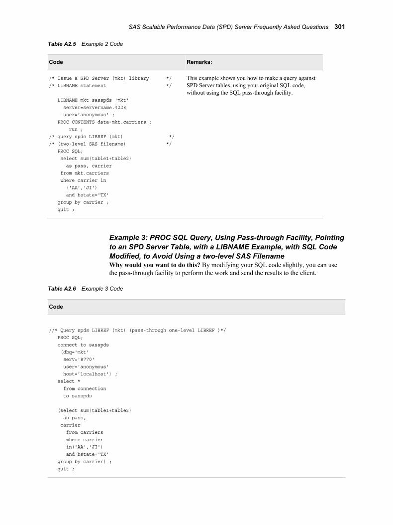
Table A2.5 Example 2 Code
Code Remarks:
/* Issue a SPD Server (mkt) library *//* LIBNAME statement */
LIBNAME mkt sasspds 'mkt' server=servername.4228 user='anonymous' ; PROC CONTENTS data=mkt.carriers ; run ;/* query spds LIBREF (mkt) *//* (two-level SAS filename) */ PROC SQL; select sum(table1+table2) as pass, carrier from mkt.carriers where carrier in ('AA','JI') and bstate='TX' group by carrier ; quit ;
This example shows you how to make a query against SPD Server tables, using your original SQL code, without using the SQL pass-through facility.
Example 3: PROC SQL Query, Using Pass-through Facility, Pointing to an SPD Server Table, with a LIBNAME Example, with SQL Code Modified, to Avoid Using a two-level SAS FilenameWhy would you want to do this? By modifying your SQL code slightly, you can use the pass-through facility to perform the work and send the results to the client.
Table A2.6 Example 3 Code
Code
//* Query spds LIBREF (mkt) (pass-through one-level LIBREF )*/ PROC SQL; connect to sasspds (dbq='mkt' serv='8770' user='anonymous' host='localhost') ; select * from connection to sasspds
(select sum(table1+table2) as pass, carrier from carriers where carrier in('AA','JI') and bstate='TX' group by carrier) ; quit ;
SAS Scalable Performance Data (SPD) Server Frequently Asked Questions 301

Example 4: PROC SQL Query, Using the Pass-through Facility, Pointing to an SPD Server Table, Executing a Libref Statement on the Server, So That Existing Code Can Be Used "as Is"Why would you want to do this? Without modifying your SQL code, you can use the pass-through facility so that SPD Server performs the work and sends the results to the client.
Table A2.7 Example 4 Code
Code
PROC SQL ; connect to sasspds (dbq='mkt' serv='8770' user='anonymous' host='localhost'); /* Issue passthru LIBREF (mkt) for use */ /* in two-level queries */ execute(LIBREF mkt) by sasspds; /* Query the SPD Server LIBREF (mkt) */ /* that is a pass-through LIBREF */ select * from connection to sasspds
(select sum(table1+table2) as pass, carrier from mkt.carriers where carrier in('AA','JI') and bstate='TX' group by carrier) ; quit;
Can I use pass-through async to create multiple indexes on a single existing table?
No. Multiple create indexes on the same existing table are not supported with async.
PROC DATASETS can be used to create indexes in parallel for a single existing table.
For example:
PROC DATASETS lib=foo ;modify customer( asyncindex=yes index=(state) ;index create state ;index create phoneno ;index create custno ;index create totsales ;quit ;
302 Appendix 2 • SAS Scalable Performance Data (SPD) Server Frequently Asked Questions
Can I use pass-through async to create multiple indexes on existing tables?
Yes. As long as you create only one index per table, the index creation can be run with async.
For example, to create an index State on table Customer, an index Totals on table Billing, and an index Orderno on table Orders asynchronously, you use the following code:
execute(begin async operation) by sasspds ;
execute(create index state on customer(state)) by sasspds ;
execute(create index totals on billing(totals)) by sasspds ;
execute(create index orderno on orders(orderno)) by sasspds ;
execute(end async operation) by sasspds ;
What size increases can I expect for tables that are stored in domains with BACKUP=YES?
Tables created in domains that have Backup=YES will have an additional 17 bytes per observation.
What files are created in the SPD Server WORKPATH directory?Some SPD Server operations can create temporary files that are too large to fit in memory. The SPD Server WORKPATH directory contains these temporary files. The temporary files in the WORKPATH directory are also called spill files, because SPD Server spills intermediate files from volatile memory to a temporary file. Temporary files in the WORKPATH directory are removed when the operation that generated the temporary file completes. There are four types of temporary that SPD Server can store in the WORKPATH directory:
Parallel Sort Spill FilesWhen SPD Server sorts a table, it uses multiple concurrent threads to sort portions of the table in memory. Each thread creates a sort bin to which it can spill temporary results files to. When the sort threads complete, the sort bin contents are merged to produce the final result. The sort bin files are named using the following convention:
spdssr_<pid>_<unique_thread_id>.0.0.0.spds9
pid is the identifier for the SPDSBASE user proxy that is performing the parallel sort operation.
Parallel GROUP BY Spill FilesWhen SPD Server performs a parallel GROUP BY operation, it uses multiple concurrent threads to group intermediate results in parallel. Each thread creates a sort bin to which it can spill temporary results files to. When the GROUP BY threads
SAS Scalable Performance Data (SPD) Server Frequently Asked Questions 303

complete, the sort bin contents are merged to produce the final result. The GROUP BY bin files are named using the following convention:
spdspgb_<pid>_<unique_thread_id>.0.0.0.spds9
pid is the identifier for the SPDSBASE user proxy that is performing the parallel GROUP BY operation.
Parallel Join Spill FilesWhen SPD Server performs a parallel join operation, it uses multiple concurrent threads to join portions of the table in memory. Each thread creates a join bin to which it can spill temporary results files to. When the parallel join threads complete, the join bin contents are merged to produce the final result. The join bin files are named using the following convention:
spdspllj_<pid>_<unique_thread_id>.0.0.0.spds9
pid is the identifier for the SPDSBASE user proxy that is performing the parallel join operation.
SQL Temporary Work FilesSPD Server creates temporary work space files for SQL operations that require intermediate results to be spilled to a workspace file. These temporary workspace files are named using the following convention:
spds_<pid>_<unique_id>.0.0.0.spds9
pid is the identifier for the SPDSBASE SQL proxy that created the temporary workspace file.
Debug Log FilesSPD Server can create temporary work space files that contain SPD Server debugging information. The debugging information can be found in the SPD Server SAS log, under headings such as “WHERE Debug” or “SQL Planning.” These temporary workspace files are generally small and are named using the following convention:
spdslog_<pid>_<unique_id>.0.0.0.spds9
pid is the identifier for the SPDSBASE user proxy that created the temporary workspace file.
How can I identify the spdsbase user proxy processes for a given SPD Server user?
The spdsbase process contains identifier start-up parameters. The start-up parameters can be used to determine which SPD User submitted the command to create a particular proxy process.
• The first parameter is the SPD Server User ID that the spdsbase proxy process was created on behalf of.
• The second parameter is the operating system User ID of the client that the spdsbase proxy process was created on behalf of.
• The fifth parameter is the IP address of the client that the spdsbase proxy process was created on behalf of.
You can display spdsbase process parameter information by submitting the command ps -ef in UNIX, or by viewing the command line information in Windows task manager.
304 Appendix 2 • SAS Scalable Performance Data (SPD) Server Frequently Asked Questions

Appendix 3
SAS Scalable Performance Data (SPD) Server SQL Syntax Reference Guide
SPD Server SQL Syntax . . . . . . . . . . . . . . . . . . . . . . . . . . . . . . . . . . . . . . . . . . . . . . . 306
Document Conventions . . . . . . . . . . . . . . . . . . . . . . . . . . . . . . . . . . . . . . . . . . . . . . . 306Productions . . . . . . . . . . . . . . . . . . . . . . . . . . . . . . . . . . . . . . . . . . . . . . . . . . . . . . . 306Literal Text . . . . . . . . . . . . . . . . . . . . . . . . . . . . . . . . . . . . . . . . . . . . . . . . . . . . . . . 306Optional Text . . . . . . . . . . . . . . . . . . . . . . . . . . . . . . . . . . . . . . . . . . . . . . . . . . . . . 306Selection Lists . . . . . . . . . . . . . . . . . . . . . . . . . . . . . . . . . . . . . . . . . . . . . . . . . . . . . 306
SQL Syntax Definitions . . . . . . . . . . . . . . . . . . . . . . . . . . . . . . . . . . . . . . . . . . . . . . . 306Statement or Query . . . . . . . . . . . . . . . . . . . . . . . . . . . . . . . . . . . . . . . . . . . . . . . . . 306Scalar Expressions and Boolean Predicates . . . . . . . . . . . . . . . . . . . . . . . . . . . . . . 307Strings . . . . . . . . . . . . . . . . . . . . . . . . . . . . . . . . . . . . . . . . . . . . . . . . . . . . . . . . . . . 307Identifiers . . . . . . . . . . . . . . . . . . . . . . . . . . . . . . . . . . . . . . . . . . . . . . . . . . . . . . . . 308Reserved Keywords . . . . . . . . . . . . . . . . . . . . . . . . . . . . . . . . . . . . . . . . . . . . . . . . 308
SQL Statements . . . . . . . . . . . . . . . . . . . . . . . . . . . . . . . . . . . . . . . . . . . . . . . . . . . . . 308ALTER TABLE Statement . . . . . . . . . . . . . . . . . . . . . . . . . . . . . . . . . . . . . . . . . . . 308ASYNC OPERATION Statement . . . . . . . . . . . . . . . . . . . . . . . . . . . . . . . . . . . . . 308CONNECT Statement . . . . . . . . . . . . . . . . . . . . . . . . . . . . . . . . . . . . . . . . . . . . . . 309COPY TABLE Statement . . . . . . . . . . . . . . . . . . . . . . . . . . . . . . . . . . . . . . . . . . . . 309CREATE INDEX Statement . . . . . . . . . . . . . . . . . . . . . . . . . . . . . . . . . . . . . . . . . 309CREATE MATERIALIZED VIEW Statement . . . . . . . . . . . . . . . . . . . . . . . . . . . 309CREATE TABLE Statement . . . . . . . . . . . . . . . . . . . . . . . . . . . . . . . . . . . . . . . . . 309CREATE VIEW Statement . . . . . . . . . . . . . . . . . . . . . . . . . . . . . . . . . . . . . . . . . . 309DELETE Statement . . . . . . . . . . . . . . . . . . . . . . . . . . . . . . . . . . . . . . . . . . . . . . . . 310DESCRIBE TABLE Statement . . . . . . . . . . . . . . . . . . . . . . . . . . . . . . . . . . . . . . . 310DESCRIBE VIEW Statement . . . . . . . . . . . . . . . . . . . . . . . . . . . . . . . . . . . . . . . . . 310DISCONNECT Statement . . . . . . . . . . . . . . . . . . . . . . . . . . . . . . . . . . . . . . . . . . . 310DROP INDEX Statement . . . . . . . . . . . . . . . . . . . . . . . . . . . . . . . . . . . . . . . . . . . . 310DROP TABLE Statement . . . . . . . . . . . . . . . . . . . . . . . . . . . . . . . . . . . . . . . . . . . . 310DROP VIEW Statement . . . . . . . . . . . . . . . . . . . . . . . . . . . . . . . . . . . . . . . . . . . . . 311EXECUTE Statement . . . . . . . . . . . . . . . . . . . . . . . . . . . . . . . . . . . . . . . . . . . . . . . 311INSERT Statement . . . . . . . . . . . . . . . . . . . . . . . . . . . . . . . . . . . . . . . . . . . . . . . . . 311LIBREF Statement . . . . . . . . . . . . . . . . . . . . . . . . . . . . . . . . . . . . . . . . . . . . . . . . . 311LOAD TABLE Statement . . . . . . . . . . . . . . . . . . . . . . . . . . . . . . . . . . . . . . . . . . . 311RESET Statement . . . . . . . . . . . . . . . . . . . . . . . . . . . . . . . . . . . . . . . . . . . . . . . . . . 311SELECT Statement . . . . . . . . . . . . . . . . . . . . . . . . . . . . . . . . . . . . . . . . . . . . . . . . . 312TRUNCATE TABLE Statement . . . . . . . . . . . . . . . . . . . . . . . . . . . . . . . . . . . . . . 312UPDATE Statement . . . . . . . . . . . . . . . . . . . . . . . . . . . . . . . . . . . . . . . . . . . . . . . . 312VALIDATE Statement . . . . . . . . . . . . . . . . . . . . . . . . . . . . . . . . . . . . . . . . . . . . . . 312
SQL Building Blocks . . . . . . . . . . . . . . . . . . . . . . . . . . . . . . . . . . . . . . . . . . . . . . . . . 312
305

SPD Server SQL SyntaxSPD Server SQL is a dialect of SQL. It combines SQL-92, SAS SQL, and extensions that are specific to SPD Server. Whenever possible, SPD Server attempts to conform to SAS SQL.
Document Conventions
ProductionsThe syntax uses building blocks that are called productions. Productions are denoted by the symbol ::= . To the left of the symbol is a production name; to the right of the symbol, or on the next line, is a list of production constructs. If a production has more than one possible construct, the alternatives are separated by a vertical bar |. Read productions top-down. For example, the delete statement contains literal keywords and two subproductions, a table specification, and then a WHERE clause.
Literal TextTraversing down a syntax tree leads to leaf or terminal definitions. The definitions consist of either keywords, identifiers (names of tables, columns, and so on), or symbols (punctuation, operators, and so on). Keywords and identifiers are shown with capitalized text. In contrast, symbols are shown with single quotation marks and are bold.
Optional TextOptional syntax is delimited by square brackets ([ ]). Optional lists (syntax elements that are repeated) are denoted by square brackets, followed by an asterisk (*). The * signifies zero or more occurrences of the bracketed syntax.
Selection ListsSelection lists, which enable you to choose from a list of alternative syntax elements, are denoted by braces ({ }). The alternative elements are separated by a vertical bar (|). The selection list itself is not optional; you must choose at least one element. When you specify one or more elements, the list is terminated with a closing brace and a plus sign (}+). The + indicates one or more occurrences of the delimited syntax.
SQL Syntax Definitions
Statement or QueryOne or more syntax elements terminated by a semicolon.
306 Appendix 3 • SAS Scalable Performance Data (SPD) Server SQL Syntax Reference Guide
Scalar Expressions and Boolean PredicatesScalar expressions represent a single data value, either a numeric value or a string from a constant specification. Examples include:
• 1
• 'hello there'
• '31-DEC-60'd)
• a function [for example, avg(a*b)]
• a column or variable (for example, foo.bar)
• the case expression
• a subquery that returns a single run-time value
.
Boolean predicates are either true or false. They are used in WHERE clauses, having clauses, and in the case expression. You cannot select predicates, nor can you assign them to columns (that is, in an update statement). Scalar expressions and Boolean predicates cannot be used interchangeably, although you can mix the expressions in SAS SQL.
StringsSPD Server SQL strings are character streams that are delimited by either single or double quotation marks. If you use a single quotation mark to begin a string, you must use a single quotation mark to terminate the string. To embed a single quotation mark in a string, use two single quotation marks together:
SELECT 'it''s a wonderful life' from mytable.
You can use double quotation marks in the same way. You can use double quotation marks as delimiters:
SELECT "it's a wonderful life" from mytable.
Some of the SQL syntax specifications in this chapter reference user-defined or database-specific strings. Delimit these strings in brackets or parentheses. Characters between the delimiters are considered part of the string up to, but not including, the matching delimiter.
CONNECT to sasspds( user='john' passwd='foobar' options=(a b c) );
The dbms_options string is
user='john' passwd='foobar' options=(a b c).
SQL Syntax Definitions 307
In this example, the first opening parenthesis is considered part of the string. It is not the matching termination delimiter.
IdentifiersIdentifiers are the names of librefs, tables, indexes and columns, as well as table and column aliases.
Reserved KeywordsYou use keywords to initiate statements and syntax elements, for example, WHERE or GROUP BY clauses. Keywords are reserved. You cannot use them for identifiers because this use introduces ambiguity. For example, select unique from; is a valid but ambiguous statement. The following list contains current SPD Server keywords. Some of the words are reserved for future enhancements to SPD Server SQL.
add, all, alter, and, any, as, asc, async, begin, between, both, by,calculated, cascade, case, char, character, column, connect,connection, contains, contents, copy, corr, corresponding, create,cross, date, dec, decimal, default, delete, desc, describe,dictionary, disconnect, distinct, double, drop, else, end, engname,engopt, eq, except, execute, exists, false, float, for, format, from,full, ge, grant, group, gt, having, in, index, indexes, informat,inner, insert, int, integer, intersect, into, is, join, label, le,leading, left, libref, like, load, lower, lt, match, missing, modify,natural, ne, no, not, notin, null, num, numeric, on, operation, option,or, order, outer, overlaps, partial, precision, privileges, public,real, references, reset, restrict, revoke, right, select, set,smallint, some, table, then, to, trailing, trim, true, union, unique,unknown, update, upper, using, validate, values, varchar, verbose,view, when, where, with, without, yes
SQL Statements
ALTER TABLE StatementThe ALTER TABLE statement changes a table definition.
alter table statement ::= ALTER TABLE table spec { { ADD|MODIFY|ALTER [ COLUMN ] column def list } | { DROP [ COLUMN ] column name list } }+ ';'
ASYNC OPERATION StatementThe ASYNC OPERATION statement controls the begin and end of asynchronous processing.
async operation statements ::= { BEGIN | END } ASYNC OPERATION ';'
308 Appendix 3 • SAS Scalable Performance Data (SPD) Server SQL Syntax Reference Guide

CONNECT StatementThe CONNECT statement creates a pass-through connection.
connect statement ::= CONNECT TO libref name [ [ AS ] alias name ] '(' dbms options ')' ] ';'
COPY TABLE StatementUse the COPY TABLE statement to copy tables.
copy table statement ::= COPY TABLE table spec FROM table spec [ WITHOUT INDEXES ] [ORDER BY column name [ ASC | DESC ] [',' column name [ ASC | DESC ]]] ';'
CREATE INDEX StatementThe CREATE INDEX statement creates an index on a table.
create index statement ::= CREATE [ UNIQUE ] INDEX index name ON table spec '(' column name list ')' ';'
CREATE MATERIALIZED VIEW StatementUse the CREATE MATERIALIZED VIEW statement to create a materialized view of a table.
create materialized view statement ::= CREATE MATERIALIZED VIEWtable spec ASselect spec ';'
CREATE TABLE StatementThe CREATE TABLE statement creates a table definition.
create table statement ::= CREATE TABLE table spec { '(' column def list ')' | ASselect spec | LIKEtable spec } ';'
CREATE VIEW StatementThe CREATE VIEW statement creates a view on one or more tables.
create view statement ::= CREATE VIEW
SQL Statements 309
table spec ASselect spec ';'
DELETE StatementThe DELETE statement deletes records.
delete statement ::= DELETE FROMtable spec [where clause ] ';'
DESCRIBE TABLE StatementThe DESCRIBE TABLE statement describes a table definition.
describe table statement ::= DESCRIBE TABLE table spec [ [','] table spec ]* ';'
DESCRIBE VIEW StatementThe DESCRIBE VIEW statement describes a view definition.
describe view statement ::= DESCRIBE VIEW table spec [ [','] table spec ]* ';'
DISCONNECT StatementThe DISCONNECT statement is a pass-through statement.
disconnect statement ::= DISCONNECT FROMlibref name ';'
DROP INDEX StatementThe DROP INDEX statement drops an index from a table.
drop index statement ::= DROP INDEX index name [ [','] index name ]* FROM table spec ';'
DROP TABLE StatementThe DROP TABLE statement drops a table definition.
drop table statement ::= DROP TABLEtable spec [ [',']table spec ]* ';'
310 Appendix 3 • SAS Scalable Performance Data (SPD) Server SQL Syntax Reference Guide

DROP VIEW StatementThe DROP VIEW statement drops a view definition.
drop view statement ::= DROP VIEW table spec [ [','] table spec ]* ';'
EXECUTE StatementThe EXECUTE statement is a pass-through statement.
execute statement ::= EXECUTE '('passthru spec ')' BYlibref name ';'
INSERT StatementThe INSERT statement adds records.
insert statement ::= INSERT INTO table spec [ '(' column name list ')' ] insert source ';'
LIBREF StatementUse the libref statement to assign LIBNAME domains for the SQL server.
LIBREF statement ::= LIBREF libref name [ ENGNAME '=' identifier ] [ ENGOPT '=' string ] ';'
LOAD TABLE StatementUse the LOAD TABLE statement to specify a table to load.
load table statement ::= LOAD TABLE table spec [ WITH with index spec [ ',' with index spec ]* ] AS select spec ';'
RESET StatementThe RESET statement resets session options and flags.
set option statement ::= { SET OPTION | RESET } { identifier [ '=' { constant |
SQL Statements 311

identifier |truth value| DEFAULT } ] }+
SELECT StatementThe SELECT statement retrieves information.
select statement::=select spec ';'
TRUNCATE TABLE StatementThe TRUNCATE TABLE statement drops a table definition.
truncate teble statement::= TRUNCATE TABLEtable spec [ [',']table spec ]* ';'
UPDATE StatementThe UPDATE statement updates records.
update statement ::= UPDATE table spec SET column name '='scalar expr [ ','column name '='scalar expr ]* [ where clause ] ';'
VALIDATE StatementThe VALIDATE statement validates a given SELECT specification.
validate statement ::= VALIDATEselect spec ';'
SQL Building BlocksAlias Name
alias name ::=identifier
Atomic Expression
atomic expr ::=constant |column spec
Between Predicate
312 Appendix 3 • SAS Scalable Performance Data (SPD) Server SQL Syntax Reference Guide
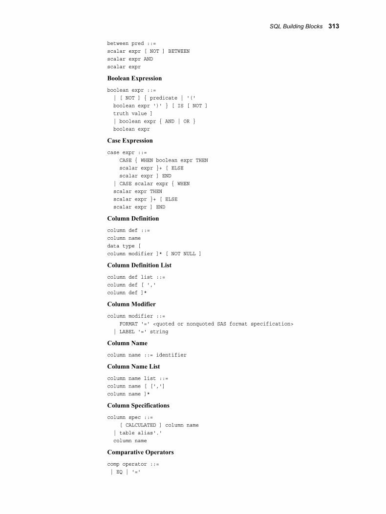
between pred ::=scalar expr [ NOT ] BETWEENscalar expr ANDscalar expr
Boolean Expression
boolean expr ::= | [ NOT ] { predicate | '(' boolean expr ')' } [ IS [ NOT ] truth value ] | boolean expr { AND | OR } boolean expr
Case Expression
case expr ::= CASE { WHEN boolean expr THEN scalar expr }+ [ ELSE scalar expr ] END | CASE scalar expr { WHEN scalar expr THEN scalar expr }+ [ ELSE scalar expr ] END
Column Definition
column def ::=column namedata type [column modifier ]* [ NOT NULL ]
Column Definition List
column def list ::=column def [ ','column def ]*
Column Modifier
column modifier ::= FORMAT '=' <quoted or nonquoted SAS format specification> | LABEL '=' string
Column Name
column name ::= identifier
Column Name List
column name list ::=column name [ [',']column name ]*
Column Specifications
column spec ::= [ CALCULATED ] column name | table alias'.' column name
Comparative Operators
comp operator ::= | EQ | '='
SQL Building Blocks 313
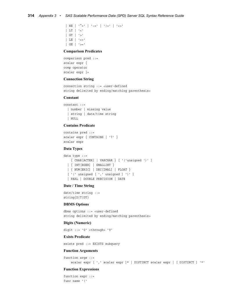
| NE | '^=' | '~=' | '!=' | '<>' | LT | '<' | GT | '>' | LE | '<=' | GE | '>='
Comparison Predicates
comparison pred ::=scalar expr {comp operatorscalar expr }+
Connection String
connection string ::= <user-definedstring delimited by ending/matching parenthesis>
Constant
constant ::= | number | missing value | string | date/time string | NULL
Contains Predicate
contains pred ::=scalar expr { CONTAINS | '?' }scalar expr
Data Types
data type ::= { CHAR[ACTER] | VARCHAR } [ '('unsigned ')' ] | { INT[EGER] | SMALLINT } | { NUM[ERIC] | DEC[IMAL] | FLOAT } [ '(' unsigned [ ',' unsigned ] ')' ] | REAL | DOUBLE PRECISION | DATE
Date / Time String
date/time string ::=string{D|T|DT}
DBMS Options
dbms options ::= <user-definedstring delimited by ending/matching parenthesis>
Digits (Numeric)
digit ::= '0' <through> '9'
Exists Predicate
exists pred ::= EXISTS subquery
Function Arguments
function args ::= scalar expr [ ',' scalar expr ]* | DISTINCT scalar expr | [ DISTINCT ] '*'
Function Expressions
function expr ::=func name '('
314 Appendix 3 • SAS Scalable Performance Data (SPD) Server SQL Syntax Reference Guide
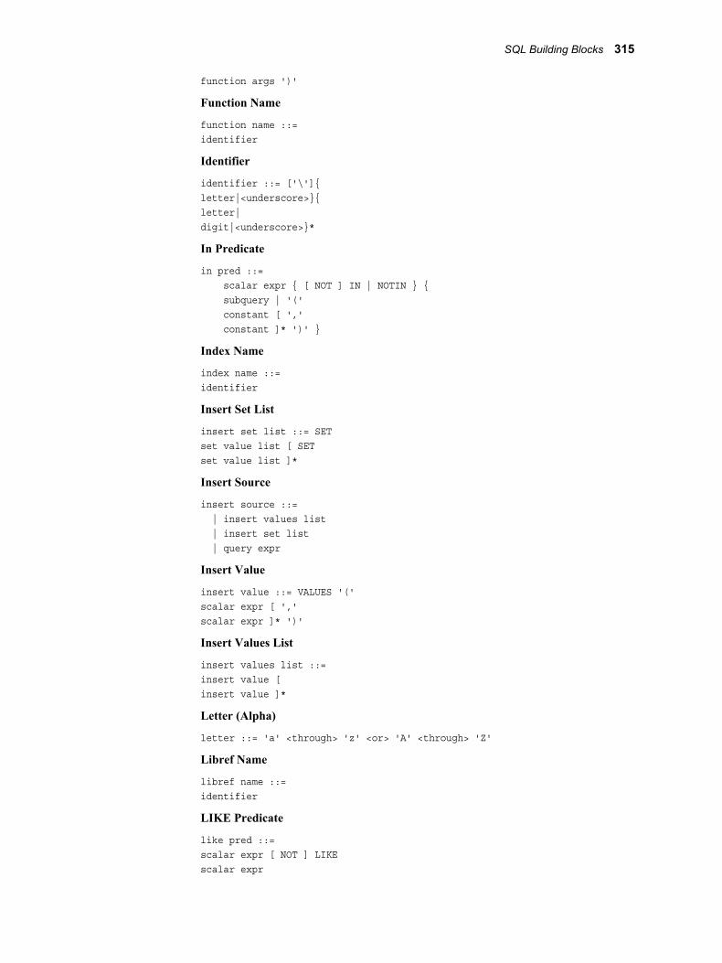
function args ')'
Function Name
function name ::=identifier
Identifier
identifier ::= ['\']{letter|<underscore>}{letter|digit|<underscore>}*
In Predicate
in pred ::= scalar expr { [ NOT ] IN | NOTIN } { subquery | '(' constant [ ',' constant ]* ')' }
Index Name
index name ::=identifier
Insert Set List
insert set list ::= SETset value list [ SETset value list ]*
Insert Source
insert source ::= | insert values list | insert set list | query expr
Insert Value
insert value ::= VALUES '('scalar expr [ ','scalar expr ]* ')'
Insert Values List
insert values list ::=insert value [insert value ]*
Letter (Alpha)
letter ::= 'a' <through> 'z' <or> 'A' <through> 'Z'
Libref Name
libref name ::=identifier
LIKE Predicate
like pred ::=scalar expr [ NOT ] LIKEscalar expr
SQL Building Blocks 315
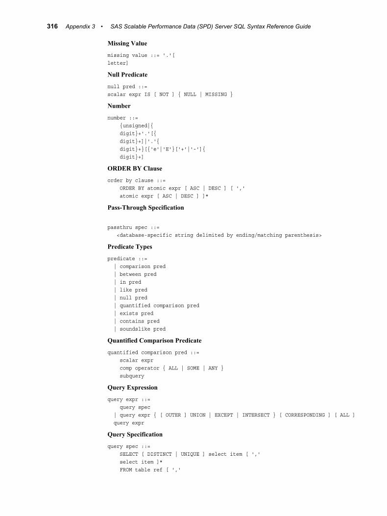
Missing Value
missing value ::= '.'[letter]
Null Predicate
null pred ::=scalar expr IS [ NOT ] { NULL | MISSING }
Number
number ::= {unsigned|{ digit}+'.'[{ digit}+]|'.'{ digit}+}[{'e'|'E'}['+'|'-']{ digit}+]
ORDER BY Clause
order by clause ::= ORDER BY atomic expr [ ASC | DESC ] [ ',' atomic expr [ ASC | DESC ] ]*
Pass-Through Specification
passthru spec ::= <database-specific string delimited by ending/matching parenthesis>
Predicate Types
predicate ::= | comparison pred | between pred | in pred | like pred | null pred | quantified comparison pred | exists pred | contains pred | soundslike pred
Quantified Comparison Predicate
quantified comparison pred ::= scalar expr comp operator { ALL | SOME | ANY } subquery
Query Expression
query expr ::= query spec | query expr { [ OUTER ] UNION | EXCEPT | INTERSECT } [ CORRESPONDING ] [ ALL ] query expr
Query Specification
query spec ::= SELECT [ DISTINCT | UNIQUE ] select item [ ',' select item ]* FROM table ref [ ','
316 Appendix 3 • SAS Scalable Performance Data (SPD) Server SQL Syntax Reference Guide

table ref ]* [ WHERE boolean expr ] [ GROUP BY scalar expr [ ',' scalar expr ]* ] [ HAVING boolean expr ]
Scalar Expression
scalar expr ::= | atomic expr | function expr | '(' scalar expr ')' | subquery | scalar expr { '+' | '-' | '*' | '/' | '||' | '**' }scalar expr | { '+' | '-' } scalar expr | case expr
Select Item
select item ::= '*' | identifier'.*' | scalar expr [ [ AS ] identifier ] [ column modifier ]*
Select Specification
select spec ::=query expr [order by clause ]
Set Value List
set value list ::=column name '='scalar expr [ ','column name '='scalar expr ]*
Soundslike Predicate
soundslike pred ::=scalar expr '=*'scalar expr
String
string ::=<a single- or double-quotedliteral string -- see Strings>
Subquery
subquery ::= '('query expr
Table Alias
table alias ::=identifier
Table Join
SQL Building Blocks 317

table join ::= table ref [ INNER | { LEFT | RIGHT | FULL } [ OUTER ] ] JOIN table ref { ON boolean expr | USING '('column name list ')' } | '(' table join ')'
Table Name
table name ::=identifier
Table Options
table options ::= <user-defined string delimited by ending/matching bracket>
Table Reference
table ref ::= table spec [ [ AS ] identifier ] | subquery [ [ AS ] identifier ] [ '(' column name list ')' ] | CONNECTION TO identifier '(' connection string ')' [ [ AS ] identifier ] | table join
Table Specification
table spec ::= | table name [ '[' table options ']' ] | libref name'.' table name [ '[' table options ']' ]
Truth Value
truth value ::= { TRUE | YES } | { FALSE | NO }
Unsigned
unsigned ::= {digit }+
WHERE Clause
where clause ::= WHEREboolean expr
With Index Specification
with index spec ::= [ UNIQUE ] INDEXindex name ON '('column name list ')'
318 Appendix 3 • SAS Scalable Performance Data (SPD) Server SQL Syntax Reference Guide
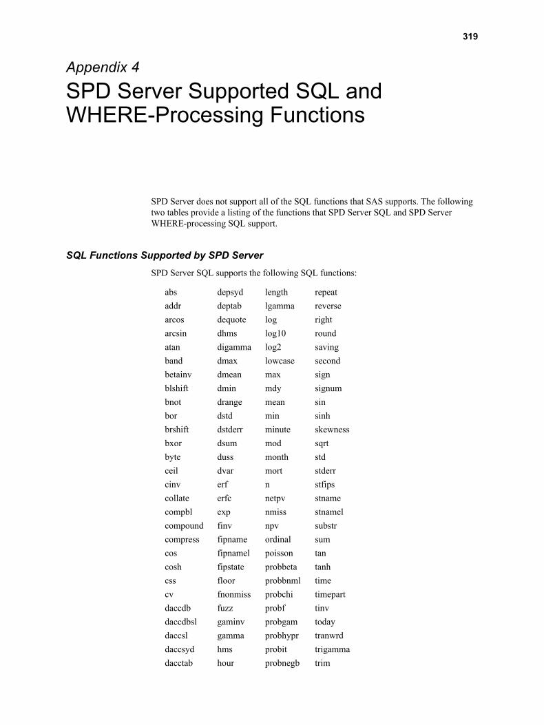
Appendix 4
SPD Server Supported SQL and WHERE-Processing Functions
SPD Server does not support all of the SQL functions that SAS supports. The following two tables provide a listing of the functions that SPD Server SQL and SPD Server WHERE-processing SQL support.
SQL Functions Supported by SPD ServerSPD Server SQL supports the following SQL functions:
abs depsyd length repeataddr deptab lgamma reversearcos dequote log rightarcsin dhms log10 roundatan digamma log2 savingband dmax lowcase secondbetainv dmean max signblshift dmin mdy signumbnot drange mean sinbor dstd min sinhbrshift dstderr minute skewnessbxor dsum mod sqrtbyte duss month stdceil dvar mort stderrcinv erf n stfipscollate erfc netpv stnamecompbl exp nmiss stnamelcompound finv npv substrcompress fipname ordinal sumcos fipnamel poisson tancosh fipstate probbeta tanhcss floor probbnml timecv fnonmiss probchi timepartdaccdb fuzz probf tinvdaccdbsl gaminv probgam todaydaccsl gamma probhypr tranwrddaccsyd hms probit trigammadacctab hour probnegb trim
319

date int probnorm upcasedatejul intck probt ussdatepart intnx put vardatetime intrr qtr weekdayday irr, quote yeardcss ispexec range zipfipsdepdb isplink ranuni zipnamedepdbsl kurtosis rank zipnameldepsl left recip zipstate
SQL WHERE-Processing Functions Supported by SPD ServerSPD Server SQL supports the following SQL WHERE-processing functions:
anyalnum dur klength permanyalpha durp kreverse pmtanycntrl effrate kright ppmtanydigit fact kscan proprobdfbbnrmanyfirst find ksubstr probmcanygraph findc ktranslate probmedanylower findw ktrim prxmatchanyname floorz kverify pvpanyprint garkhclprc largest ranbinanypunct garkhptprc lcm rancauanyspace gcd lengthc randanyupper geodist lengthm ranexpanyxdigit geomean lengthn rangamarcosh geomeanz log1px rannorarsinh gmtoff logbeta ranpoiartanh harmean mad rantblatabetan2 harmeanz margrclprc rantriblackclprc holiday margrptprc rmsblackptprc in median roundeblkshclprc index missing roundzblkshptprc indexc modz scanceilz indext nomrate scanqchoosec indexw notalnum secchoosen inputc notalpha sleepcoalesce inputn notcntrl smallestcoalescec intcindex notdigit streaminitcomb intcycle notfirst stripcompare intfit notgraph substrncompfuzz intfmt notlower sumabsconstant intget notname timevalueconvx intindex notprint translate
320 Appendix 4 • SPD Server Supported SQL and WHERE-Processing Functions
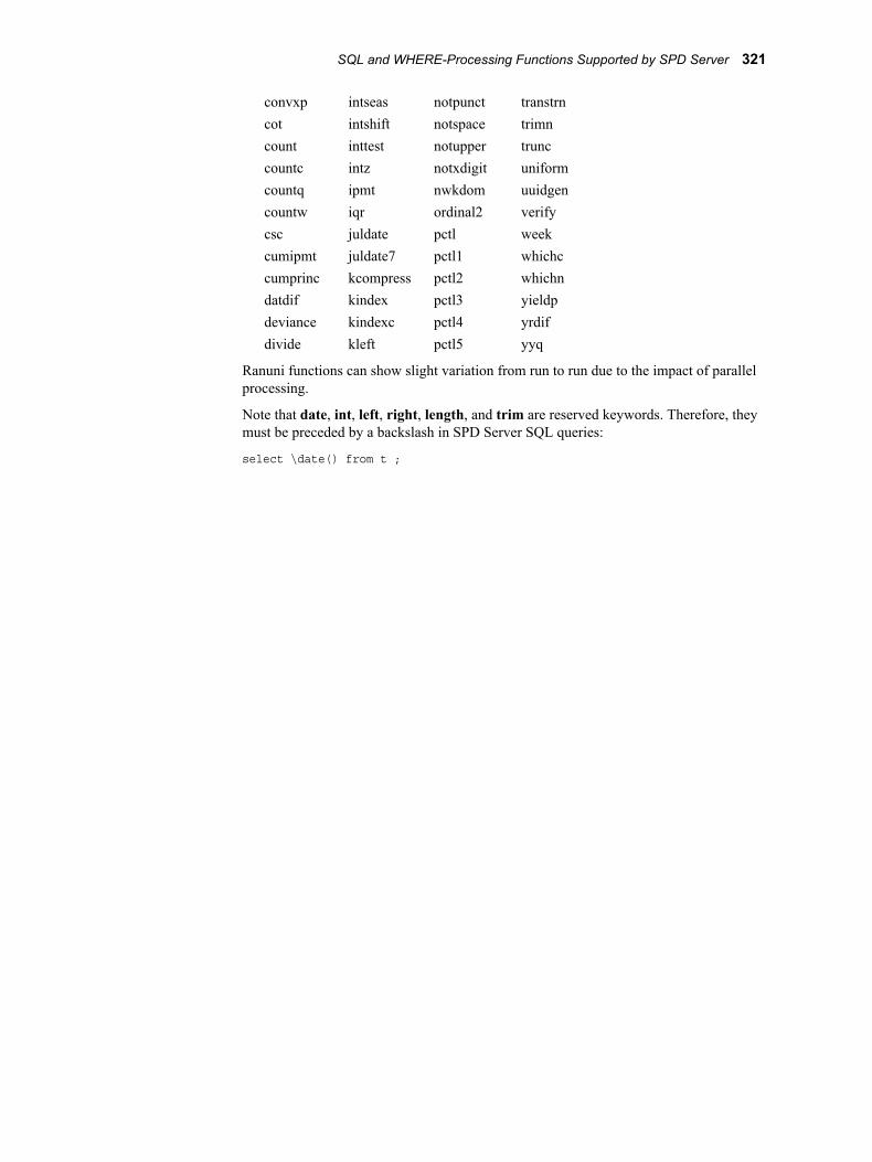
convxp intseas notpunct transtrncot intshift notspace trimncount inttest notupper trunccountc intz notxdigit uniformcountq ipmt nwkdom uuidgencountw iqr ordinal2 verifycsc juldate pctl weekcumipmt juldate7 pctl1 whichccumprinc kcompress pctl2 whichndatdif kindex pctl3 yieldpdeviance kindexc pctl4 yrdifdivide kleft pctl5 yyq
Ranuni functions can show slight variation from run to run due to the impact of parallel processing.
Note that date, int, left, right, length, and trim are reserved keywords. Therefore, they must be preceded by a backslash in SPD Server SQL queries:
select \date() from t ;
SQL and WHERE-Processing Functions Supported by SPD Server 321

322 Appendix 4 • SPD Server Supported SQL and WHERE-Processing Functions