Sampling estimators of total mill receipts for use in ... · Sampling estimators of total mill...

Sampling estimators of total mill receipts for usein timber product output studies

John P. Brown and Richard G. Oderwald

Abstract: Data from the 2001 timber product output study for Georgia was explored to determine new methods for stratify-ing mills and finding suitable sampling estimators. Estimators for roundwood receipts totals comprised several types: simplerandom sample, ratio, stratified sample, and combined ratio. Two stratification methods were examined: the Dalenius–Hodges (DH) square root of the frequency method and a cluster analysis method. Three candidate sizes for the number ofgroups were selected from the cluster analysis and subsequently used in the DH stratification as well. Relative efficiency im-proved when the number of groups increased and when using a ratio estimator, particularly a combined ratio. The two strati-fication methods performed similarly. Neither the DH method nor the cluster analysis method performed better than theother. Six bound sizes (1%, 5%, 10%, 15%, 20%, and 25%) were considered for deriving samples sizes for the total volumeof roundwood receipts. The minimum achievable bound size was found to be 10% of the total receipts volume for the DHmethod using a two-group stratification. This was true for both the stratified and combined ratio estimators. In addition, forthe stratified and combined ratio estimators, only the DH method stratifications were able to reach a 15% bound on the total(six of the 12 stratified estimators). These results demonstrate that the utilized classification methods are compatible withstratified totals estimators and can provide users with the opportunity to develop viable sampling procedures as opposed tocomplete mill censuses.

Résumé : Les données de l’étude de 2001 sur les produits de transformation du bois en Géorgie ont été analysées pouridentifier de nouvelles méthodes de stratification des usines et pour trouver des estimateurs d’échantillonnage appropriés.Quatre estimateurs du volume total des arrivages de bois rond ont été considérés : l’échantillon aléatoire simple, le rapport,l’échantillon stratifié et le rapport combiné. Deux méthodes de stratification ont été examinées : la méthode de la racine car-rée cumulée de la fréquence de Dalenius–Hodges (DH) et une méthode d’analyse par grappes. Trois tailles candidates pourle nombre de grappes ont été sélectionnées à partir de l’analyse par grappes et ensuite elles ont aussi été utilisées dans laméthode de stratification de DH. L’efficacité relative s’est améliorée avec l’augmentation du nombre de grappes et l’utilisa-tion d’un estimateur de rapport, en particulier un rapport combiné. Les deux méthodes de stratification avaient une perfor-mance similaire : la méthode de stratification de DH et la méthode d’analyse par grappes étaient équivalentes. Six tailleslimites (1 %, 5 %, 10 %, 15 %, 20 %, et 25 %) ont été considérées pour calculer la taille des échantillons pour le volume totaldes arrivages de bois rond. La taille minimale réalisable était de 10 % du volume total pour la méthode de DH basée surune stratification en deux groupes. Cette taille minimale était valable à la fois pour l’estimateur stratifié et pour l’estimateurpar rapport combiné. En outre, pour l’estimateur stratifié et l’estimateur par rapport combiné, seule la méthode de stratifica-tion de DH a pu atteindre la limite de 15 % du volume total (six des 12 estimateurs stratifiés). Ces résultats démontrent queles méthodes de classification utilisées sont compatibles avec les estimateurs des totaux stratifiés et peuvent fournir aux utili-sateurs l’occasion de développer des méthodes d’échantillonnage viables par opposition au recensement complet des usines.

[Traduit par la Rédaction]

Introduction

Periodic assessments of timber removals are an importantcomponent of the US Forest Service’s national forest inven-tory and monitoring program. One method of assessment isthe timber product output (TPO) survey, which is conductedunder the direction of each US Forest Service research sta-tion’s forest inventory and analysis (FIA) program. During aTPO survey, a complete canvass of all primary wood-usingmills is conducted in a state. The primary measure of interestis roundwood receipts, which is the cubic foot volume of

roundwood harvested in the state plus roundwood importedfrom other states. The data collected provide important infor-mation on the amount, county of harvest, and species compo-sition of roundwood harvested within each state.TPO designs vary by US Forest Service research station

and sometimes even among states within a specific researchstation’s purview. What is common to all is that a completecensus is attempted by canvassing all primary mills in eachstate (T.G. Johnson, C.E. Keegan, R.J. Piva, and E.H. Whar-ton, personal communications (2005)). Complete canvassescan be problematic due to lack of response, limited monetary

Received 31 August 2011. Accepted 29 November 2011. Published at www.nrcresearchpress.com/cjfr on 21 February 2012.

J.P. Brown. USDA Forest Service, 241 Mercer Springs Road, Princeton, WV 24740, USA.R.G. Oderwald. Department of Forest Resources and Environmental Conservation, Virginia Tech, 138 Cheatham Hall, Blacksburg, VA24061, USA.

Corresponding author: John P. Brown (e-mail: [email protected]).

476

Can. J. For. Res. 42: 476–489 (2012) doi:10.1139/X11-183 Published by NRC Research Press

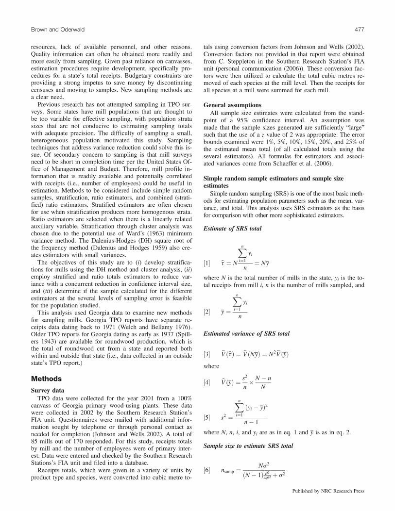
resources, lack of available personnel, and other reasons.Quality information can often be obtained more readily andmore easily from sampling. Given past reliance on canvasses,estimation procedures require development, specifically pro-cedures for a state’s total receipts. Budgetary constraints areproviding a strong impetus to save money by discontinuingcensuses and moving to samples. New sampling methods area clear need.Previous research has not attempted sampling in TPO sur-

veys. Some states have mill populations that are thought tobe too variable for effective sampling, with population stratasizes that are not conducive to estimating sampling totalswith adequate precision. The difficulty of sampling a small,heterogeneous population motivated this study. Samplingtechniques that address variance reduction could solve this is-sue. Of secondary concern to sampling is that mill surveysneed to be short in completion time per the United States Of-fice of Management and Budget. Therefore, mill profile in-formation that is readily available and potentially correlatedwith receipts (i.e., number of employees) could be useful inestimation. Methods to be considered include simple randomsamples, stratification, ratio estimators, and combined (strati-fied) ratio estimators. Stratified estimators are often chosenfor use when stratification produces more homogenous strata.Ratio estimators are selected when there is a linearly relatedauxiliary variable. Stratification through cluster analysis waschosen due to the potential use of Ward’s (1963) minimumvariance method. The Dalenius-Hodges (DH) square root ofthe frequency method (Dalenius and Hodges 1959) also cre-ates estimators with small variances.The objectives of this study are to (i) develop stratifica-

tions for mills using the DH method and cluster analysis, (ii)employ stratified and ratio totals estimators to reduce var-iance with a concurrent reduction in confidence interval size,and (iii) determine if the sample calculated for the differentestimators at the several levels of sampling error is feasiblefor the population studied.This analysis used Georgia data to examine new methods

for sampling mills. Georgia TPO reports have separate re-ceipts data dating back to 1971 (Welch and Bellamy 1976).Older TPO reports for Georgia dating as early as 1937 (Spill-ers 1943) are available for roundwood production, which isthe total of roundwood cut from a state and reported bothwithin and outside that state (i.e., data collected in an outsidestate’s TPO report.)

Methods

Survey dataTPO data were collected for the year 2001 from a 100%

canvass of Georgia primary wood-using plants. These datawere collected in 2002 by the Southern Research Station’sFIA unit. Questionnaires were mailed with additional infor-mation sought by telephone or through personal contact asneeded for completion (Johnson and Wells 2002). A total of85 mills out of 170 responded. For this study, receipts totalsby mill and the number of employees were of primary inter-est. Data were entered and checked by the Southern ResearchStations’s FIA unit and filed into a database.Receipts totals, which were given in a variety of units by

product type and species, were converted into cubic metre to-

tals using conversion factors from Johnson and Wells (2002).Conversion factors not provided in that report were obtainedfrom C. Steppleton in the Southern Research Station’s FIAunit (personal communication (2006)). These conversion fac-tors were then utilized to calculate the total cubic metres re-moved of each species at the mill level. Then the receipts forall species at a mill were summed for each mill.

General assumptionsAll sample size estimates were calculated from the stand-

point of a 95% confidence interval. An assumption wasmade that the sample sizes generated are sufficiently “large”such that the use of a z value of 2 was appropriate. The errorbounds examined were 1%, 5%, 10%, 15%, 20%, and 25% ofthe estimated mean total (of all calculated totals using theseveral estimators). All formulas for estimators and associ-ated variances come from Schaeffer et al. (2006).

Simple random sample estimators and sample sizeestimatesSimple random sampling (SRS) is one of the most basic meth-

ods for estimating population parameters such as the mean, var-iance, and total. This analysis uses SRS estimators as the basisfor comparison with other more sophisticated estimators.

Estimate of SRS total

½1� bt ¼ N

Xni¼1

yi

n¼ Ny

where N is the total number of mills in the state, yi is the to-tal receipts from mill i, n is the number of mills sampled, and

½2� y ¼

Xni¼1

yi

n

Estimated variance of SRS total

½3� bV ðbtÞ ¼ bV ðNyÞ ¼ N2bV ðyÞwhere

½4� bV ðyÞ ¼ s2

n� N � n

N

½5� s2 ¼

Xni¼1

ðyi � yÞ2

n� 1

where N, n, i, and yi are as in eq. 1 and y is as in eq. 2.

Sample size to estimate SRS total

½6� nsamp ¼ Ns2

ðN � 1Þ B2

4N2 þ s2

Brown and Oderwald 477

Published by NRC Research Press

where N is as for eq. 1, B is the error bound desired, and s2

is the population variance. This method uses s2 (eq. 5) as anestimate of s2.

Strata selection by cluster analysisCluster analysis is a statistical technique that attempts to

gather similar objects into a meaningful collection of groups.Data are collected on p variables for m objects. This analysisutilizes hierarchical clustering, one of many clustering techni-ques. The similarity matrix (or resemblance matrix) uses Eu-clidean distance. Agglomeration of clusters is based on theWard’s (1963) minimum variance linkage, with objects start-ing out singly and eventually being placed into groups basedupon minimizing the sum of the squared distances weightedby cluster size (McGarigal et al. 2000). Here, two variablesare included in the clustering: total receipts and number ofemployees. A total of 85 mills have data for both variables.A cluster analysis creates cluster sizes from one cluster —

all cases in one group — up to the n cluster — all groupssingle cases. Strict criteria for determining the number ofclusters do not exist. However, simulation studies performedby Milligan and Cooper (1985) and Cooper and Milligan(1988) indicate that the pseudo F statistic, the pseudo t2 sta-tistic, and the cubic clustering criterion (CCC) all performwell in determining the best number of clusters. Cluster sizescan be chosen by creating a scree plot of the CCC versus thenumber of clusters and examining the figure for peaks (Sarle1983). McGarigal et al. (2000) suggested a combined view ofthe CCC, pseudo F statistic, and pseudo t2 statistic wherelarge pseudo F statistics and increasing pseudo t2 statisticsfrom one cluster to the next are examined at local peaks onthe CCC scree plot. This combination then suggests a stop-ping size for the number of clusters.

Strata selection by the DH cumulative square root of thefrequency methodThe second method chosen to generate a class variable for

stratification was the DH cumulative square root of the fre-quency method (Dalenius and Hodges 1959).The DH method is another method used to generate esti-

mators with small variance. An example is provided in Ta-ble 1 using a population ranging from 0 to 1000, bin sizeb = 100, and three strata (L = 3). The DH method first binsthe observations on the response variable and a frequency ta-ble is constructed. The interval between bins is chosen by theexperimenter much like a standard histogram bin size ischosen. Once the frequencies for the bins are found, thesquare root of each frequency is taken. Then, a cumulativetotal is taken for the square roots of the frequencies. The ex-perimenter will decide how many strata are desired. The cu-mulative sum is then divided by the number of strata,arriving at a rough category size c. Stratum boundaries arethen found by picking the bins closest in cumulative fre-quency to 1·c, 2·c, ..., (L – 1)·c. For consistency, L will beset to the number of strata suggested from the clusteringanalysis.

Stratified random sample estimators and sample sizeestimatesStrata were developed using results of both the cluster

analysis and DH methods. Each method will have one or

Tab

le1.

ExamplefortheDH

method.

(1)Bins

(6)Strata

Observatio

nsy

Low

erUpper

(2)Frequency

(3)√Frequency

√Frequency

Subtotal

Low

erUpper

1610

0100

42.0

2.0

0400

2705

100

200

62.4

2.4

400

600

3959

200

300

82.8

2.8

600

1000

4127

300

400

153.9

(5)c=

30.1/3

∼10

3.9

11.1

535

400

500

214.6

4.6

6581

500

600

184.2

4.2

8.8

7810

600

700

113.3

3.3

8225

700

800

93.0

3.0

800

900

52.2

2.2

100

486

900

1000

31.7

1.7

10.2

(4)To

tal=

30.1

Note:

(1)Bin

size

100;

(2)frequenciescalculated

forbins;(3)calculatesquare

feet;(4)calculatesum

ofsquare

feet;(5)determ

inecategory

size,c

∼10;(6)find

strata

boundaries.

478 Can. J. For. Res. Vol. 42, 2012


more group size solutions. Once initial groupings are deter-mined from each method, summary statistics will be gener-ated for all groups in a solution: minimum, maximum, mean,and standard deviation. These values will help determine amodified solution that finalizes the employee ranges onwhich groups will be stratified.The modified solution ranges will be determined from the

following two procedures for each group size solution. Ifthere is no overlap in the range of the number of employeesfor a group with that of another within a solution, then theminimum and maximum numbers of employees for the con-sidered group are used as draft bounds for that group. Thesedraft bounds will be rounded to tens of employees. If there isoverlap between two groups within a solution, the boundarydivision will be determined as follows. First, take the differ-ence between the group 1 and group 2 means:

½7� d ¼ y2 � y1

Second, calculate a weight for the group one mean that is thegroup 1 standard deviation (SD) divided by the sum of theSD of group 1 and the SD of group 2:

½8� w1 ¼ s1

s1 þ s2

Third, multiply the difference of the means by the weight forgroup 1 and add that value to the group 1 mean:

½9� Upper1 ¼ w1 � d þ y1

This becomes the upper limit for group 1 and the lower limitfor group 2. Fourth, adjust this limit to reasonable tens ofemployees values. Repeat for any other overlapping groups.This method weights the distance between the strata meansand considers the overlap.Calculating sample sizes for stratified totals is more in-

volved than for a SRS. To determine the total sample size,an allocation strategy is required. The costs of obtaining amill’s information are expected to be nearly equal, yet differ-ences in strata variances are evident, so Neyman allocation isemployed to calculate the strata weights. These weights arethen incorporated into the formula for the total sample size.Strata sample sizes are obtained from multiplying out theweights and the total size.

Estimate of the stratified population total

½10� bt ¼ Nyst

where N is as for eq. 1 and

½11� yst ¼1

N

XLi¼1

Niyi

where L is the number of strata, Ni is the number of samplingunits in stratum i, and yi is the estimated mean using eq. 2for mills from stratum i.

Estimated variance of the stratified total

½12� bV ðbtÞ ¼ N2bV ðystÞ

where N is as for eq. 1,

½13� bV ðystÞ ¼ 1

N2

XLi¼1

N2i

Ni � ni

Ni

� �s2ini

where N, i, L, and Ni are as in eq. 11 and ni is the samplesize for stratum i, and

½14� s2i ¼

Xnij¼1

ðyj � yiÞ2

ni � 1

where yj is the jth observation in stratum i and yi is as in eq.11.

Neyman allocation for determining stratum allocationweight

½15� wi ¼ NisiXLk¼i

Nksk

where wi is the sample weight for stratum i, Ni (Nk) is thenumber of sampling units in stratum i (k), and si (sk) is thepopulation variance for stratum i (k). This method uses si (eq.14) as an estimate of si.

Sample size to estimate the total using stratified sampling

½16� nsamp ¼

XLi¼1

N2i s

2i =wi

B2

4þXLi¼1

Nis2i

where Ni and wi are as in eq. 15 and B is as in eq. 6. Thismethod uses s2i (eq. 14) as an estimate of s2

i .

Ratio estimators and sample size estimatesRatio estimators use a well-correlated auxiliary variable as

an aid to estimate either means or totals. Additionally, an es-timate of the population ratio may be of interest. While po-tentially biased, this bias is negligible (of the order 1/n) anddisappears if the regression of y on x (variable of interest,auxiliary variable) is a straight line through the origin(Schaeffer et al. 2006).

Estimate of the population total

½17� bt y ¼ rtx

where tx is the employee population total and

½18� r ¼

Xni¼1

yi

Xni¼1

xi



where n and yi are as in eq. 1 and xi is the number of em-ployees at mill i.

Estimate of the population variance

½19� bV ðbtyÞ ¼ t2xbV ðrÞ

where tx is as in eq. 17,

½20� bV ðrÞ ¼ N � n

N

� �1

m2x

� �s2rn

where N and n are as in eq. 1 and mx is the employee popu-lation mean, and

½21� s2r ¼

Xni¼1

ðyi � rxiÞ2

n� 1

where yi is as in eq. 1 and r and xi are as in eq. 18.

Sample size to estimate the total using a ratio estimator

½22� nsamp ¼ Ns2

B2

4Nþ s2

where N is as in eq. 1 and s2 and B are as in eq. 6. Thismethod uses s2r (eq. 21) as an estimate of s2.

Stratified ratio estimators (combined)The two varieties of stratified ratio estimators are separate

ratio estimators and combined ratio estimators (Schaeffer etal. 2006). Separate ratio estimators estimate r (sample ratio)within the strata and these strata estimates for r are then com-bined with weighted strata means and totals to arrive at pop-ulation estimates for the mean or total. The combined ratioestimator estimates r from the stratified means of both thevariable of interest and its auxillary variable. The combinedestimate for r is then used with the weighted stratum meansor totals to arrive at the desired population estimates.For small sample sizes within strata, it is recommended

that the combined ratio estimator be used (Schaeffer et al.2006). For larger sample sizes, the separate estimator gener-ally provides narrower confidence intervals, especially whenstrata ratios differ markedly. This analysis will use combinedratio estimators due to smaller sample sizes. Sample sizes forthe combined ratio estimator are calculated similarly to thoseof the stratified estimator (eq. 6) with the exception that s2ri isused to estimate s2

i (as opposed to using s2i (eq. 5)).

Estimate of population total

½23� bt yC ¼ ystxsttx

where xst is the stratified mean for mill employees using eq.11, yst is as in eq. 11, and tx is as in eq. 17.

Estimated variance of population total

½24� bV ðbtyCÞ ¼ N2bV ðbmyCÞwhere N is as in eq. 1,

½25� bV ðbmyCÞ ¼XLi¼1

Ni

N

� �2Ni � ni

Ni

� �s2rini

where L, Ni, and ni are as in eq. 11,

½26� s2ri ¼

Xnij¼1

ðyij � rCxijÞ2

ni � 1

where xij is the number of employees for mill j from stratum iand yij is the cubic metres total for mill j from stratum i, and

½27� rC ¼ ystxst

where xst and yst are as in eq. 23.

Sample size to estimate the total using a ratio estimatorCalculations utilize eq. 16 with the exception that s2ri is

used to estimate s2i (as opposed to using s2i (eq. 14)).

Comparison of estimatorsTotals for each of the estimators were calculated using the

85 responding mills. Variances for each of the estimatorswere compared using the estimated relative efficiency

½28� cRE E1

E2

� �¼

bV ðE1ÞbV ðE2Þwhere E1 and E2 are estimators and bV ðE1Þ and bV ðE2Þ are therespective estimated variances.

Results

Cluster analysis stratification and estimatorsValues for the CCC indicated a local peak at two clusters

with a plateau approached at six clusters (Fig. 1). Cluster

Cu

bic

clu

ster

ing c

rite

rion

-1

0

1

2

Number of clusters

1 2 3 4 5 6

Sta

tist

ic v

alu

e

0

50

100

150

200

250

300CCC Pseudo F Pseudo t2

Fig. 1. CCC, pseudo F, and pseudo t2 values for the cluster analysis.

480 Can. J. For. Res. Vol. 42, 2012


numbers of larger than six were rejected due to insufficientpotential sample sizes within clusters. The pseudo t2 andpseudo F statistics suggested two, four, and six groups; thepseudo t2 statistic showed local peaks at four and six, whilethe pseudo F had higher values at two, four, five, and six.Therefore, the data were divided into groups of two, four,and six by liberally considering all criteria.The stratification of mills into groups when sampling will

ultimately be based solely on the number of employees.While the receipts data are a useful auxiliary variable, theyare unknown before sampling (particularly for new mills),whereas the employee data are easily obtainable. This con-straint necessitated examining the cluster solution and devel-oping a stratification that modified the original clusteranalysis group characteristics. Prior mill receipts data arereadily obtainable, as most states have previous TPO data.Future mill stratifications can therefore be conducted on arange of employee values that potentially have incorporatedsome information from the previous receipts relationship. Inthe event that prior receipt data are not available, a pilotstudy could be conducted.The employee ranges obtained from modifying the original

cluster solution are presented in Table 2. Note that for thesix-group cluster solution, a sixth group was not obtainablebased on the distribution of groups from the initial clustering.There is separation in two dimensions, but not reasonableseparation along the employee dimension. Therefore, themodified cluster solution has five groups as the largest groupsize examined and is referred to as the six/five-group solu-tion.The sample variances for the various groups formed from

clustering into two, four, and six/five groups are presented inFig. 2. Several groups had variances smaller than1.00 × 1010. These are the groups shown as gaps in the fig-ure. The majority of the groups had variances less than thatfor the SRS variance, with only five out of the 23 groups ex-ceeding this value.

DH method stratification and estimatorsThe divisions that led to the groupings by the DH method

are presented in Table 3. Bin sizes of 1 million ft3 were usedto develop groupings. Once the cumulative square root of the

frequencies (CSQRTF) was calculated, group divisions weremade.As an example, consider the four-group solution. The

CSQRTF is 37.72, which is divided by 4. This results in aninterval of around 9.4. Divisions are then made at 9.38,18.77, and 27.65, creating four categories of mill sizes. Thereare 47, 13, 12, and 13 mills in each category, respectively.This grouping provides a reasonable number of mills perstratum (and it does so for the other two group sizes as well).The employee ranges obtained from modifying the original

cluster solution are presented in Table 4. There were no is-sues with overlapping groups, as this method used one varia-ble to separate the groups.The sample variances for the two-, four-, and six-group

stratifications for both the DH solution and the modified DHsolution along with the SRS variance are presented in Fig. 3.Again, several of the variances near or below the value 1.0 ×1010 do not appear in the figure. Similar to the cluster solu-tions, the majority of the variances are below the value forthe SRS solution, with only six out of 24 groups having var-iances greater than that of the SRS solution.

Table 2. Cluster analysis group statistics and solution ranges based on number of employees.

Cluster solution Modified cluster solution

No. ofgroups Group Minimum Maximum Mean SD Minimum Maximum2 1 1 381 73.22 91.48 1 400

2 400 907 691.00 159.71 401 9074 1 1 66 20.90 17.15 1 40

2 37 381 168.15 95.21 41 3303 400 907 657.83 188.50 331 7304 692 800 757.33 57.46 731 907

6/5 1 1 66 20.90 17.15 1 502 37 169 113.05 37.45 51 2003 240 381 299.12 47.13 201 3604 400 826 597.50 183.44 361 7205 692 800 757.33 57.46 720 9076 650 907 778.50 181.73

Cluster solution Mod. cluster solution SRS

Va

ria

nce

(m

)3

2

0.00E+00

1.00E+11

2.00E+11

3.00E+11

4.00E+11

5.00E+11

6.00E+11

7.00E+11

Two groups Four groups Six/five groups SRS

Fig. 2. Sample variances for the cluster, modified cluster, and SRSgroupings. Gaps indicate strata with variances too small to plot.



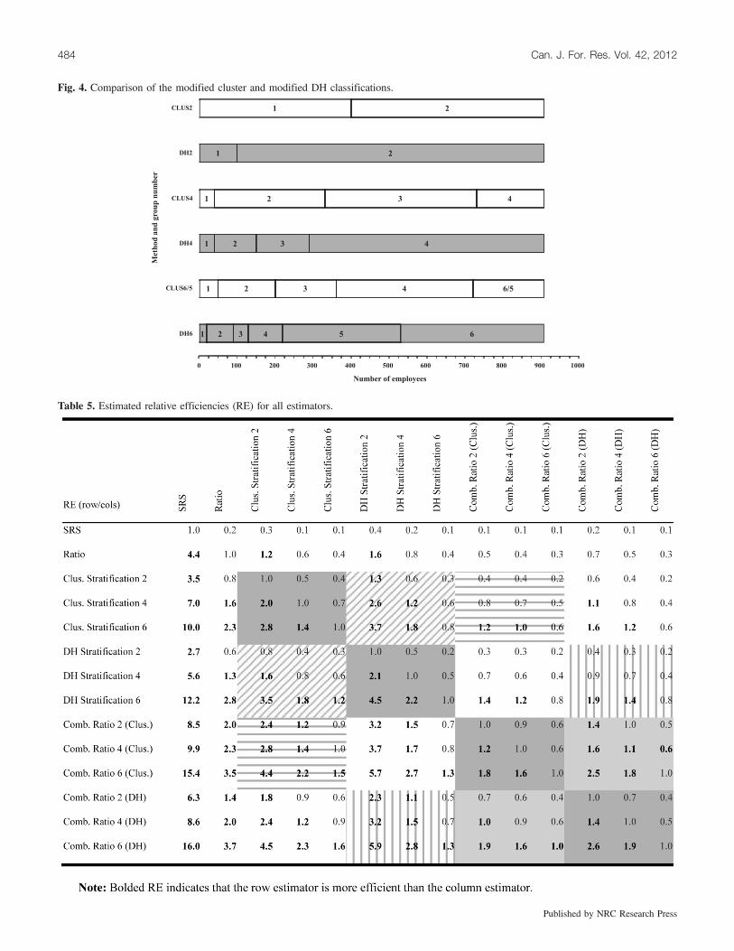
Comparison of the modified cluster and DHclassificationsThe employee ranges obtained for the groupings in both

the DH and cluster classifications differed when consideringthe same number of groups. The two-group solution for thecluster analysis was divided nearly in the middle of the em-

Table 3. DH method cutoff values for two-, four-, and six-group sizes.

Table 4. DH method group statistics and solution ranges based on number of employees.

DH solution Modified DH solution

No. ofgroups Group Minimum Maximum Mean SD Minimum Maximum2 1 1 285 40.30 54.12 1 100

2 70 907 374.64 270.58 101 9074 1 1 103 21.04 19.59 1 40

2 17 285 109.92 78.92 41 1503 70 381 193.33 103.43 151 2904 150 907 542.00 270.94 291 907

6 1 1 40 13.51 10.95 1 202 14 285 58.69 64.17 21 903 37 240 111.78 61.71 91 1304 70 381 167.00 108.66 131 2205 134 826 328.70 231.72 221 5306 400 907 677.58 174.59 531 907

482 Can. J. For. Res. Vol. 42, 2012


ployee range, while the DH method had a much lower breakat about 100 employees (Fig. 4). For the larger number ofgroups, four and six/five, the cluster solution exhibited moreeven employee ranges in its group sizes. The DH solutionhad variable employee ranges among the strata for both thefour- and six-strata solutions.The modified cluster solution generally has group varian-

ces higher than those of the cluster solution, although itshould be noted that the groups do not always comprise thesame mills. The groups having the greatest number of em-ployees tended to have the highest variances, and those ofthe modified cluster solution were larger than those of thecluster solution. The two-group solution had the greatest sim-ilarity between the cluster solution and the modified clustersolution.

Relative efficiencies of estimatorsThe estimated relative efficiencies of the estimators are in-

cluded in Table 5. Efficiencies greater than 1 suggest that theestimator in the row position of the table is more efficientthat the estimator in the column. However, it should be notedthat these are calculated variances and not theoretical varian-ces, and any differences may be due to random chance.Many comparisons are presented in Table 5. The number

of groups is the foremost factor to consider, and these com-parisons are possible at many levels: within a stratificationmethod and type of means analysis (e.g., DH method, strati-fied mean analysis), across stratification methods (e.g., clus-ter stratification versus DH stratification), and across meansmethods (cluster stratified mean versus combined ratio (clus-ter)).First, consider the comparisons for group size within a

stratification method and type of means analysis. These arefound in the 3 × 3 blocks (dark gray blocks) along the maindiagonal of Table 5. For each of the four combinations pro-duced from crossing stratification method and means method(e.g., combined ratio (cluster)), relative efficiency improvesfor increasing numbers of groups. That is, six groups aremore efficient than four groups, which are more efficientthan two groups, and these relationships are transitive.

Next, group sizes can be compared within the stratifiedmean method. When comparing the cluster method with theDH method within stratified means, the relative efficienciesrange from 0.8 to 1.3 (Table 5, main diagonals within diago-nal striped blocks). A similar range in relative efficiencies,0.7–1.4, results for the cluster versus DH comparison withinthe combined ratio method (Table 5, main diagonals withinlight gray blocks).The final group size comparison considered is across

means methods. Comparing the cluster analysis methodacross means methods (Table 5, main diagonals, horizontalstriped blocks), relative efficiency ranges from 0.4 to 2.4.For the DH method, the range across means methods is 0.4–2.3 (Table 5, main diagonals within vertical striped blocks).The last set of comparisons is each individual estimator

versus the SRS (Table 5, first column). All estimators havegreater than 1 relative efficiency versus the SRS. Addition-ally, all specific stratification and means method types showincreasing efficiency versus the SRS with increasing groupsize.

Confidence intervals for totalsThe 95% confidence intervals for the totals of the various

methods range from a lower limit of 1.07 billion ft3 to a highof 2.10 billion ft3 (Fig. 5). Confidence interval ranges arenarrowest for the combined ratio estimators, while the clusterand DH stratified totals are slightly broader. The widest inter-val (1.26, 2.10) billion ft3 is that of the SRS.

Estimated sample sizes for SRS and ratio totalsSRS sample sizes ranged downwards from 170 to 82 to

achieve bounds of 1%–25% of the total state receipts (volumeof logs) (Fig. 6). (Strictly speaking, the 170 sample sizewould force a total census.) Ratio sample sizes ranged from169 down to 44 for the same bounds. Ratio sample sizeswere less than SRS sample sizes for all considered bounds.

Estimated sample sizes for stratified totalsStratum weights were calculated for all strata in each of

the stratification methods using the class sample standard de-viation estimates and the number of sampling units availablefor each stratum (Table 6). One important factor here is thebreakdown of stratum sampling units into the classes gener-ated from the two stratification methods. The cluster analysissolutions have, in all cases, one stratum with 10 or fewermills. Further, within both the four and six/five classifications,there is a stratum with only four sampling units available.The estimated strata standard deviations obtained from the

two stratification methods differ among classes almost exclu-sively by no more than 1 order of magnitude. The DH 6 sol-ution is the only one where this is not true and samplestandard deviations differ by 2 orders of magnitude.Weights for both stratification methods range from 0.05 to

0.86, with most weights ranging from 0.10 to 0.25. TheCluster 2 solution Stratum 1 weight is the greatest and theDH 6 Stratum 1 weight is the smallest. The Cluster 4 Stra-tum 2 and DH 4 Stratum 4 weights, at 0.55 and 0.43, arethe most dissimilar within all of the solutions (Table 6).These weights are then used to calculate the stratum sam-

ple sizes needed for each method from the calculated totalsample size necessary for each bound (Fig. 7). Due to a finite

DH Solution Mod. DH Solution SRS

Va

ria

nce

(m

)3

2

0.00E+00

1.00E+11

2.00E+11

3.00E+11

4.00E+11

5.00E+11

6.00E+11

7.00E+11

Two groups Four groups Six groups SRS

Fig. 3. Sample variances for the DH, modified DH, and SRS group-ings. Gaps indicate strata with variances too small to plot.



1

1

1

1

1

1

2

2

2

2

2

2

3

3

3

3

4

4

4

4

5

6/5

6

0 100 200 300 400 500 600 700 800 900 1000

DH6

CLUS4

Number of employees

Met

hod

an

d g

rou

p n

um

ber

Fig. 4. Comparison of the modified cluster and modified DH classifications.

Table 5. Estimated relative efficiencies (RE) for all estimators.

484 Can. J. For. Res. Vol. 42, 2012


population, several stratum sample size estimates exceededthe total number of sampling units in the stratum and arenoted in bold in Table 6 and as stippled columns in Fig. 7.Sample size estimates are highest at 150 for the 1% bound

of the cluster stratification two-group solution. The lowest

sample size needed is 14 for the 25% bound on the DH strat-ification six-group solution. Sample sizes decrease, as ex-pected, as bound size increases and also decrease as thenumber of groups used to estimate the total increases(Fig. 7).

0

1

2

3

SR

S

Rati

o

Clu

s. S

trati

fica

tion

2

Clu

s. S

trati

fica

tion

4

Clu

s. S

trati

fica

tion

6

DH

Str

ati

fica

tion

2

DH

Str

ati

fica

tion

4

DH

Str

ati

fica

tion

6

Com

b. R

ati

o 2

(C

lus.

)

Com

b. R

ati

o 4

(C

lus.

)

Com

b. R

ati

o 6

(C

lus.

)

Com

b. R

ati

o 2

(D

H)

Com

b. R

ati

o 4

(D

H)

Com

b. R

ati

o 6

(D

H)

Cu

bic

fee

t (b

illi

on

s)

Fig. 5. Estimates for total receipts by all methods.

0

20

40

60

80

100

120

140

160

180

1% 5% 10% 15% 20% 25%

Nu

mb

ero

f m

ills

Bound (% of total)

Ratio SRS

Fig. 6. Ratio and SRS estimated sample sizes for state totals from a population of 170 mills.



Estimated sample sizes for combined ratio totalsThe division of sampling units is the same for each stratum

here, as was noted previously (e.g., the cluster analysis clas-sification into four groups produces the same sample frame).What differs between Table 6 and Table 7 are the estimatesfor each group’s variance.The estimated stratum standard deviations vary from 1 to 2

orders of magnitude within stratification solutions. Here, boththe Cluster 4 and DH 6 solutions have the widest ranges inestimated standard deviations (Table 7).Weights range from a low of 0.05 to 0.78 for the DH 6

Stratum 1 and Cluster 2 Stratum 1 strata, respectively.Weights are again in the 0.10–0.25 range, with some minordeviations from those weights as happened in the stratifica-tions shown in Table 6.Sample sizes were again highest at 117 for the cluster

stratification into two groups (Fig. 8). The lowest samplesize of 12 was for the DH stratification into six groups. Theweights and stratum sample sizes calculated to estimate thecombined ratio totals also result in several strata sample sizesthat are unattainable (Table 7, bold values).

Discussion

Classification methods group rangesThere were clear differences between the employee ranges

for each group obtained by the cluster method and those ob-tained by the DH method. There were many groups with nar-row ranges for the DH method, whereas there is moreuniformity of employee ranges for the cluster solutions withinspecific group size solutions, e.g., CLUS2 (Fig. 4). This is

unexpected, as it was thought that the DH method mightlead to more uniform groupings due to the initial binning ofobservations.This difference in employee range sizes within the DH sol-

ution also leads to more groups for mills with fewer employ-ees. That is not unexpected because the method naturallyconcentrates high frequencies into narrow range categories.Stated differently, the CSQRTF is divided into a set numberof intervals, with each interval a fixed fraction of the totalCSQRTF. Increasing the number of similar observations forthe variable of interest will force the determined range to benarrower. That stands to be a useful technique if the variableof interest is strongly correlated with the auxiliary variableused to classify into strata.

Group sizesThere is a clear increase in estimator efficiency with in-

creasing group size within specific stratification and meansmethods (Table 5, dark gray cells). The stratifications byboth the cluster and DH methods allow for a decrease in var-iability within the groups formed by the methods. The cRE(six groups/two groups) was greatest in all instances, with ahigh of 4.5 calculated for the DH stratification. For the Stateof Georgia, stratification into four or six groups appears to bea reasonable approach to reducing estimator variance.Group size is an important factor in reducing the number

of samples needed to achieve the several bounds examined(Figs. 2 and 3). All of the cluster method by means methodcombinations show a decrease in the necessary sample sizesas the number of groups employed in the stratification in-creases.

Table 6. Stratum sample sizes for state stratified totals.

Sample size for several bounds

Stratum Ni SD Weight 1% 5% 10% 15% 20% 25%Cluster 2 1 160 8.28E+06 0.86 128 120 98 76 58 44

2 10 2.24E+07 0.14 22 20 17 13 10 8Cluster 4 1 91 1.08E+06 0.11 8 8 6 4 3 2

2 63 7.90E+06 0.55 43 39 30 21 15 113 12 1.70E+07 0.22 17 16 12 9 6 54 4 2.78E+07 0.12 10 9 7 5 3 3

Cluster 6/5 1 101 1.07E+06 0.13 9 8 6 4 3 22 46 7.56E+06 0.43 30 27 20 14 10 73 11 8.69E+06 0.12 8 7 5 4 3 24 8 1.82E+07 0.18 13 11 8 6 4 35 4 2.78E+07 0.14 10 9 6 5 3 2

DH 2 1 123 3.84E+06 0.33 31 29 25 21 17 132 47 2.08E+07 0.67 64 61 53 43 34 27

DH 4 1 91 1.08E+06 0.10 7 7 5 4 3 22 49 7.26E+06 0.36 27 24 19 15 11 83 11 8.64E+06 0.10 7 7 5 4 3 24 19 2.25E+07 0.44 32 29 23 18 13 10

DH 6 1 66 5.53E+05 0.05 3 3 2 1 1 12 50 3.28E+06 0.22 16 14 10 7 5 33 16 5.76E+06 0.12 9 8 5 4 3 24 15 8.00E+06 0.16 11 10 7 5 3 25 16 1.12E+07 0.24 17 15 11 7 5 46 7 2.34E+07 0.22 16 14 10 7 5 3

Note: Values in bold indicate that the stratum sample size exceeds the stratum size.

486 Can. J. For. Res. Vol. 42, 2012


Stratification methodsComparison of the stratification methods for similar group

sizes can be considered within a means method, i.e., strati-fied or ratio estimator. For these data, neither the cluster northe DH method appears to be more efficient (Table 5, diago-nals within diagonal striped and light gray cells). The relativeefficiencies for these comparisons are close to 1. Therefore,neither method is recommended over the other based on thismeasure. However, the stratification itself is an improvementin efficiency over the SRS estimator and in most cases overthe simple ratio estimator.There were few differences in sample size estimates for the

two stratification methods (cluster and DH). The differenceswere nearly immeasurable for the four- and six-group solu-tions within any means method. However, there were some-what larger differences when comparing sample sizeestimates for the DH two-group solutions with the clustersolutions for the stratified total (Fig. 7). Differences for thesecomparisons occurred again for the combined ratio samplesize estimates (Fig. 8). These differences in the two-groupsolution may be a result of only having two groups and thatthe cluster solution had an unbalanced distribution of sam-pling units within its two strata: N1 = 170 and N2 = 10.

Totals methodsBy holding the stratification method and group size con-

stant, we can examine the effect of the totals method. Here,there appears to be a clear advantage to using a combined ra-tio estimator versus a regular stratified mean (Table 5, diago-nals within horizontal striped cells and vertical striped cells).Relative efficiencies range upward from 1.3, thereby indicat-ing that the additional information contained within the em-ployee numbers is providing smaller variances on theestimate of the total. In addition, the much simpler compari-son for the cRE (ratio/SRS) yields an efficiency of 4.4 (Ta-ble 5), further evidence that the number of employees is auseful auxiliary variable.There is a marked reduction in the number of samples

needed for a fixed group size and stratification method whenswitching from a stratified total to a combined ratio total innearly all cases (Figs. 7 and 8). Giving specific considerationto the fact that some bound sizes produce unattainable stra-tum sample sizes, at least 20% more samples are needed bythe ordinary stratification total to achieve the same bound asthe combined ratio total.The DH 2 method using combined ratio estimators produ-

ces the only sampling strategy where a 10% bound on the to-tal is attainable. Further, the DH method for the combinedratio estimator is the only method by which 15% bounds onthe total are attainable (all group size solutions). All methodscan be used if a 20% bound is an acceptable range for thetotal.

0

20

40

60

80

100

120

140

160

180

1% 5% 10% 15% 20% 25%

Nu

mb

erof

mil

ls

Bound (% of total)

DH Strat 6

Cluster Strat 6

DH Strat 2

Cluster Strat 2

Fig. 7. Stratified estimated sample sizes for state totals from a population of 170 mills. Stippled columns indicate that one or more stratumsample sizes exceed the stratum for that particular method.



Table 7. Stratum sample sizes for state combined ratio totals.

Sample size for several bounds

Stratum Ni SD Weight 1% 5% 10% 15% 20% 25%Cluster 2 1 160 4.95E+06 0.78 92 81 60 41 29 20

2 10 2.19E+07 0.22 25 22 16 11 8 6Cluster 4 1 91 9.78E+05 0.11 8 7 5 4 3 2

2 63 7.03E+06 0.55 41 36 26 18 13 93 12 1.27E+07 0.19 14 13 9 6 4 34 4 2.98E+07 0.15 11 10 7 5 3 3

Cluster 6/5 1 101 1.02E+06 0.15 10 8 6 4 3 22 46 6.09E+06 0.40 26 23 16 11 7 53 11 7.31E+06 0.12 7 7 5 3 2 24 8 1.37E+07 0.16 10 9 6 4 3 25 4 2.98E+07 0.17 11 10 7 4 3 2

DH 2 1 123 2.45E+06 0.32 30 26 20 14 10 72 47 1.37E+07 0.68 63 57 42 30 21 16

DH 4 1 91 9.81E+05 0.11 8 7 5 4 3 22 49 5.56E+06 0.34 25 22 16 11 8 63 11 1.09E+07 0.15 11 10 7 5 4 34 19 1.74E+07 0.41 31 27 20 14 10 7

DH 6 1 66 4.88E+05 0.05 3 3 2 1 1 12 50 2.51E+06 0.19 12 10 7 5 3 23 16 5.59E+06 0.14 9 7 5 3 2 24 15 7.97E+06 0.18 12 10 7 5 3 25 16 8.02E+06 0.19 13 11 7 5 3 26 7 2.37E+07 0.25 16 14 10 6 4 3

Note: Values in bold indicate that the stratum sample size exceeds the stratum size.

0

20

40

60

80

100

120

140

160

180

1% 5% 10% 15% 20% 25%

Nu

mb

erof

mil

ls

Bound (% of total)

DH Strat 6

Cluster Strat 6

DH Strat 2

Cluster Strat 2

Fig. 8. Combined ratio estimated sample sizes for state totals from a population of 170 mills. Stippled columns indicate that one or morestratum sample sizes exceed the stratum for that particular method.

488 Can. J. For. Res. Vol. 42, 2012


ConclusionNew approaches to conducting TPO studies demonstrate

that statistical estimation procedures can be of benefit to gen-erating estimates for a state’s mill receipts. Results from thisanalysis indicate that stratification, coupled with ratio estima-tors based on employee numbers at mills, can greatly reducethe variance of estimated totals. These reductions will allowfor an expected reduction in the number of samples neededto achieve desired bounds on a state’s receipts total.Stratification and the use of auxiliary information are de-

monstrably useful techniques in achieving reasonable boundson a state’s total receipts data. Slightly better results are pro-duced using the DH stratification method, allowing forbounds of 15% of the estimated total for both means meth-ods, as opposed to the cluster method attaining only the 20%level. The use of a combined ratio total estimator allows for asignificant reduction in the necessary sample size. For thesedata, the easily obtained value for the total number of em-ployees provides a much greater benefit through stratificationversus using a SRS estimator. Given that most states haveprior TPO data recorded, future sampling plans now haveworkable options should bounds be within acceptable toler-ances. Even in cases where there has not been a prior TPOstudy, a pilot study could be conducted to perform necessarystratification. In times of tighter budgets, there is consider-able value in sampling, as costs are traditionally lower thancosts for a census.

AcknowledgementsWe would like to thank Tony Johnson and Carolynn Step-

pleton, two members of the Southern Research Station FIAunit, for providing the data used in this work. Tony was in-

volved in early discussions on how to improve TPO studiesand he suggested the data used herein. Carolynn was ex-tremely helpful, gracious, and patient in helping transfer andexplain the data. Her assistance was invaluable.

ReferencesCooper, M.C., and Milligan, G.W. 1988. The effect of measurement

error on determining the number of clusters in cluster analysis. InData, expert knowledge and decisions. Edited by W. Gaul and M.Schader. Springer-Verlag, Heidelberg. pp. 319–328.

Dalenius, T., and Hodges, J.L. 1959. Minimum variance stratification.J. Am. Stat. Assoc. 54(285): 88–101. doi:10.2307/2282141.

Johnson, T.G., and Wells, J.L. 2002. Georgia’s timber industry — anassessment of timber product output and use, 1999. U.S. For. Serv.Resour. Bull. SRS68.

McGarigal, K., Cushman, S., and Stafford, S. 2000. Multivariatestatistics for wildlife and ecology research. Springer-Verlag, NewYork.

Milligan, G.W., and Cooper, M.C. 1985. An examination ofprocedures for determining the number of clusters in a data set.Psychometrika, 50(2): 159–179. doi:10.1007/BF02294245.

Sarle, W. 1983. Cubic clustering criterion. SAS® Tech. Rep. A-108.SAS® Institute, Inc., Cary, N.C.

Schaeffer, R.L., Mendenhall, W., and Ott, R.L. 2006. Elementarysurvey sampling. 6th ed. Thomson Brooks/Cole, Belmont, Calif.

Spillers, A.R. 1943. Georgia forest resources and industries. U.S. For.Serv. Misc. Publ. 501.

Ward, J.H., Jr. 1963. Hierarchical grouping to optimize an objectivefunction. J. Am. Stat. Assoc. 58(301): 236–244. doi:10.2307/2282967.

Welch, R. L.; Bellamy, T. R. 1976. Changes in output of industrialtimber products in Georgia, 1971–1974. U.S. For. Serv. Resour.Bull. SE-RB-36.



Sampling estimators of total mill receipts for use in ... · Sampling estimators of total mill...

Documents

Transcript of Sampling estimators of total mill receipts for use in ... · Sampling estimators of total mill...