Sampling Distribution of the

Sample Proportion

N(0,1)

zStandardized

height (no units)

Sampling dist. of sample Prop = Distribution of p

Distribution of X:

z =(x− )

Let X=height or height. X ~ N(,)

Q: To find Probability with

common three steps:

Step 1. Standardize; That is, to

find Z-score;

Step2: Draw N(0, 1) and shade;

Step3: Find:

Prob=Area

=NCDF(low, high, 0, 1)

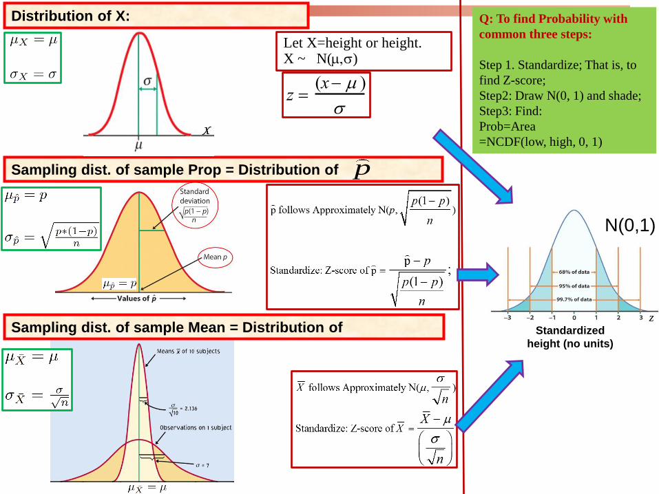
Sampling dist. of sample Mean = Distribution of

Exact N( , ) Exact N( , )

Not Exact Normal, but with Approximately N( , )

Mean and SD

Distribution of X, (n=1): Sampling distribution of , (n>1) :

,

X

n

n

(By Central Limit Theorem)

Standardize: Z-score of Reverse: ; *X Xn

XZ

n

= = +

−

3

Sampling distribution of a sample mean=distribution of X

Population

Simple random sample (SRS)

Data are summarized by statistics

(mean, standard deviation, median,

quartiles, correlation, etc..)

Concerns:

1) Is sample proportion related to population proportion?

2) If yes, what will be the relationship? Or say, how far or how close is a sample

proportion away from the population proportion?

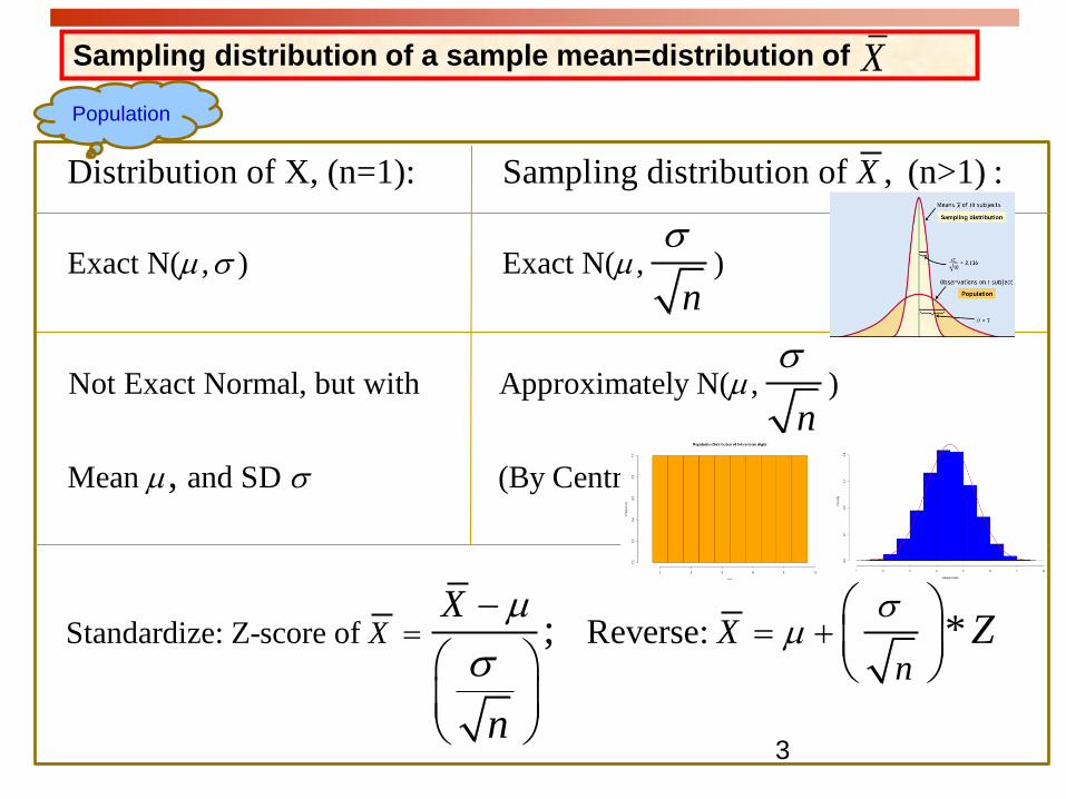
Review: Sampling proportion p-hat

Sample proportion: (p-hat, or relative frequency)

count in the samplep̂

Total=

Population proportion: p

Review: Sampling variability

Each time we take a random sample from a population, we are likely to

get a different set of individuals and calculate a different statistic. This

is called sampling variability.

If we take a lot of random samples of the same size from a given

population, the variation from sample to sample—the sampling

distribution—will follow a predictable pattern.

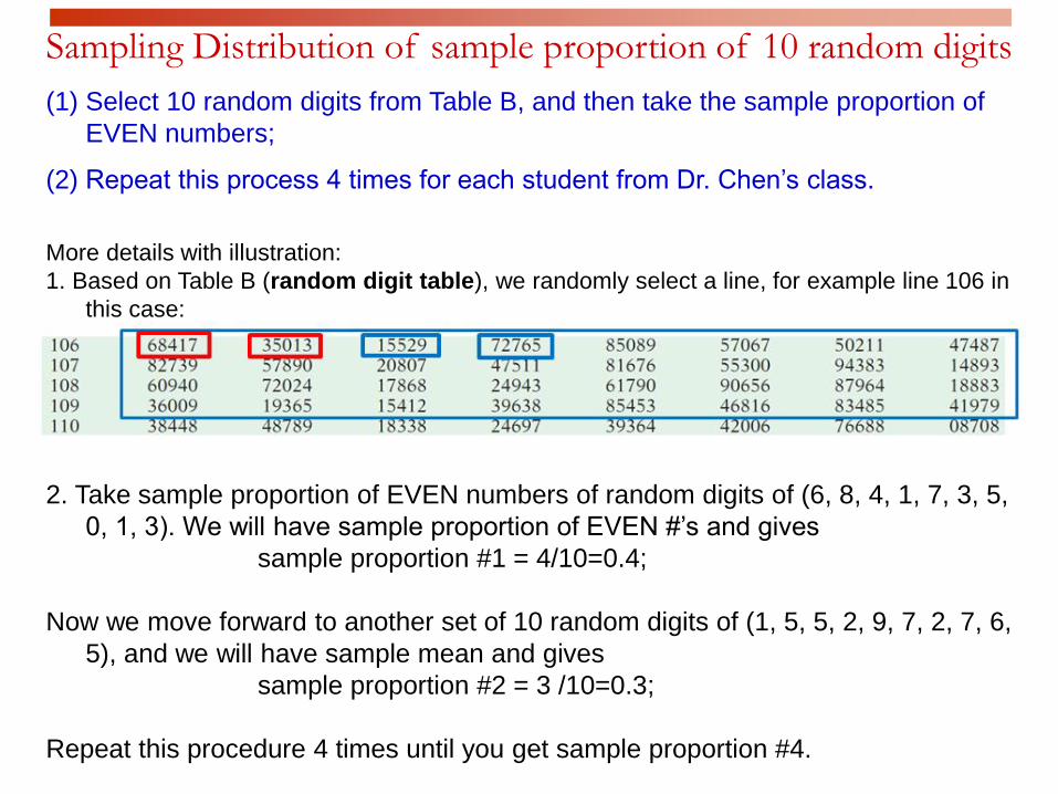
Sampling Distribution of sample proportion of 10 random digits

(1) Select 10 random digits from Table B, and then take the sample proportion of

EVEN numbers;

(2) Repeat this process 4 times for each student from Dr. Chen’s class.

More details with illustration:

1. Based on Table B (random digit table), we randomly select a line, for example line 106 in

this case:

2. Take sample proportion of EVEN numbers of random digits of (6, 8, 4, 1, 7, 3, 5,

0, 1, 3). We will have sample proportion of EVEN #’s and gives

sample proportion #1 = 4/10=0.4;

Now we move forward to another set of 10 random digits of (1, 5, 5, 2, 9, 7, 2, 7, 6,

5), and we will have sample mean and gives

sample proportion #2 = 3 /10=0.3;

Repeat this procedure 4 times until you get sample proportion #4.

For all of your p-hats:

(1)0.1

(2)0.2 0.2

(5)0.3 0.3 0.3 0.3 0.3

(21)0.4 0.4 0.4 0.4 0.4 0.4 0.4 0.4 0.4 0.4 0.4 0.4 0.4 0.4 0.4 0.4 0.4

0.4 0.4 0.4 0.4

(17)0.5 0.5 0.5 0.5 0.5 0.5 0.5 0.5 0.5 0.5 0.5 0.5 0.5 0.5 0.5 0.5 0.5

(17)0.6 0.6 0.6 0.6 0.6 0.6 0.6 0.6 0.6 0.6 0.6 0.6 0.6 0.6 0.6 0.6 0.6

(7)0.7 0.7 0.7 0.7 0.7 0.7 0.7

(5)0.8 0.8 0.8 0.8 0.8

(1)0.9

Q: Draw a histogram with classes as: (for line 101-120 in Table B)

Sampling Distribution of sample mean of 10 random digits

Class (0, 0.1] (0.1, 0.2] (0.2, 0.3] (0.3, 0.4] (0.4, 0.5] (0.5, 0.6] (0.6, 0.7] (0.7, 0.8] (0.8, 0.9]

Counts

Sampling Distribution of sample mean of 10 random digits

Class (0, 0.1] (0.1, 0.2] (0.2, 0.3] (0.3, 0.4] (0.4, 0.5] (0.5, 0.6] (0.6, 0.7] (0.7, 0.8] (0.8, 0.9]

Counts 1 2 5 21 17 17 7 5 1

Sampling

distribution

of “p hat”

Histogram

of some

sample

proportion

Q: Write a journal about how to get the

sampling distribution of Sample

proportion p-hat today, by answering the

following questions:

1) How to obtain p-hat’s from Table B for

each student?

2) How many p-hat’s did we have totally in

the class?

3) How to make a histogram for p-hat?

What is the name of the histogram?

4) What did the smooth curve represent?

5) For the smooth curve, what did the

horizontal axis and vertical axis

present?

0

8

3

74

29

5

16

Population

Sampling Distribution

38

7

4

8

36

4 98

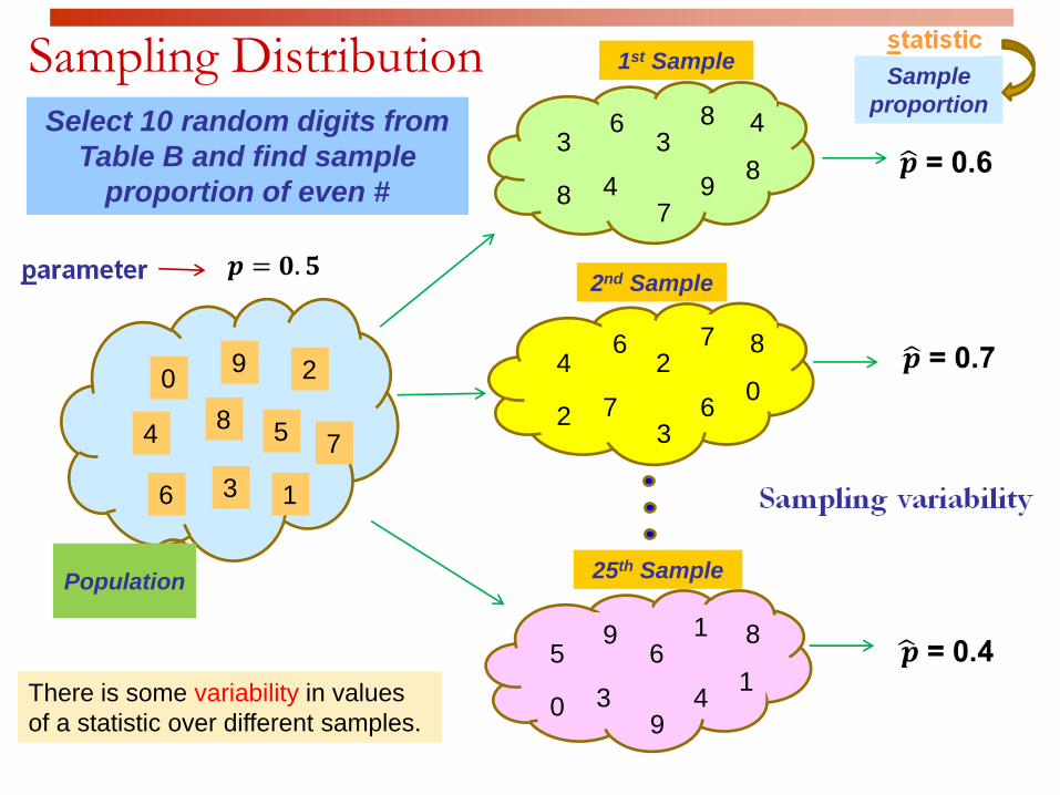
1st Sample

47

3

8

2

26

7 60

2nd Sample

25th Sample

51

9

8

0

69

3 41

Sample

proportion Select 10 random digits from

Table B and find sample

proportion of even #

There is some variability in values

of a statistic over different samples.

Sampling Distribution of sample proportion of even # of 10 random digits

(1) Select 10 random digits from Table B, and then take the sample proportion of even #.

(2) Repeat this process a lot of times, say 10,000 times.

(3) Make a histogram of these 10,000 sample mean’s. The probability distribution looks like a

Normal distribution.

Sampling

distribution

of “p-hat” Histogram

of some

“p-hat”

The probability distribution of

a statistic is called its

sampling distribution.

Center of p-hat = 0.5018

SD of p-hat = 0.1598

Note: n=10.

(1 )p p

n

−SD of p-hat =

Sampling distribution of the sample proportion

The sampling distribution of is never exactly normal. But as the sample size

increases, the sampling distribution of becomes approximately normal.

The normal approximation is most accurate for any fixed n when p is close to

0.5, and least accurate when p is near 0 or near 1.

p̂

p̂

When does the normality apply: np ≥15 and n(1 - p) ≥15

Sampling Distribution of

If data are obtained from a SRS and np>15 and n(1-p)>15, then the sampling distribution of has the following form:

For sample percentage:

is approximately normal with mean p and

standard deviation:

p̂

p̂

p̂

(1 )p p

n

−

p follows Approximately N( , )

Standardize: Z-score of p

(1 )p

(1 )

Reverse:

p

(1 );

*

p

p p

n

p p

n

p

p

p p

n

Z

=

−

−

= +

−

−

14

Sampling distribution of a sample Proportion = distribution of p

Note: data are obtained from a SRS and np>15 and n(1-p)>15.

Example 1 (a)Maureen Webster, who is running for mayor in a large city, claims that she is

favored by 53% of all eligible voters of that city. Assume that this claim is

true. In a random sample of 400 registered voters taken from this city.

Find Population proportion p= _________.

a.) What is the sampling distribution of p-hat?

b) What is the probability of getting a sample proportion less than 49% in which

will favor Maureen Webster?

c.) Find the probability of getting a sample proportion in between 50% and

55%.

d) Is it reasonable to assume Normal shape for this sampling distribution?

Explain.

(c) Z=(0.5-0.53)/0.02495 = -1.20;

Z=(0.55-0.53)/0.02495 = 0.80;

Pr(-1.20 <Z<0.80)

=normalcdf(-1.20, 0.80, 0, 1)

=0.673

(b) Z=(0.49-0.53)/0.02495 = -1.60

Pr(Z<-1.60)

=normalcdf(-E99, -1.6, 0, 1)

= 0.0548

(d) Yes.

n*p=400*0.53=212,

voting for this person.

n*(1-p) = 400*0.47=188,

voting against for this

person.

Note: data are obtained from a

SRS and np>15 and n(1-p)>15.

Example 1 (b)Maureen Webster, who is running for mayor in a large city, claims that she is

favored by 53% of all eligible voters of that city. Assume that this claim is

true. If instead we choose a random sample of 1,000 registered voters

taken from this city.

a.) What is the sampling distribution of p-hat?

b) What is the probability of getting a sample proportion less than 49% in which

will favor Maureen Webster?

(b) Z=(0.49-0.53)/0.0157829 = -2.534388

Pr(Z< -2.534388) = 0.005703126

A researcher studied the use of prenatal care among low-income

American women. She found that only 51 percent of these women

had adequate prenatal care. Let’s assume that the population of

similar low-income American women, 51 percent had adequate

prenatal care. If 200 women from this population are drawn at

random, what is the probability that less than 45 percent will have

received adequate prenatal care?

Example 2:

𝑝 = 0.51 𝑛 = 200 Ƹ𝑝 = 0.45

𝜇 ො𝑝 = 𝑝 = 0.51

𝜎 ො𝑝 =𝑃 1 − 𝑃

𝑛

=0.51 0.49

200

= 0.0353

𝑧 ො𝑝 =Ƹ𝑝 − 𝑝

𝜎 ො𝑝

=0.45 − 0.51

0.0353= −1.7

𝑃( Ƹ𝑝 < 0.45) = 𝑃(𝑧 ො𝑝 < −1.7)

= 𝟎. 𝟎𝟒𝟒𝟔

Researcher estimated that 64 percent of U.S. adults ages 20-74

were overweight or obese (overweight: BMI 25-29, obese: BMI 30 or

greater). Use this estimate as the population proportion for U.S.

adults ages 20-74. If 125 subjects are selected at random from the

population, what is the probability that 70 percent or more would be

found to be overweight or obese?

Example 3:

𝑝 = 0.64 𝑛 = 125 Ƹ𝑝 = 0.7

𝜇 ො𝑝 = 𝑝 = 0.64

𝜎 ො𝑝 =𝑝 1 − 𝑝

𝑛

=0.64 0.26

125

= 0.0428

𝑧 ො𝑝 =Ƹ𝑝 − 𝑝

𝜎 ො𝑝

=0.70 − 0.64

0.0428= 1.40

𝑃( Ƹ𝑝 ≥ 0.7) = 𝑃(𝑧 ො𝑝 ≥ 1.4)

= 1 − 𝑃(𝑧 ො𝑝 < 1.4)

= 1 − 0.9192 = 𝟎. 𝟎𝟖𝟎𝟖

Copyright © 2013, 2009, and 2007, Pearson Education, Inc.19

More exercise

1. 30% of all autos undergoing an emissions inspection at a city fail in the inspection. Among 200 cars randomly selected in the city, the percentage of cars that fail in the inspection is around_____, with SD______. would it be unusual to have sample percentage 35%?

2. 60% of all residents in a big city are Democrats. Among 400 residents randomly selected in the city, would it be unusual to have sample percentage percentage<58%?

3. In airport luggage screening it is known that 3% of people have questionable objects in their luggage. For the next 1600 people, use normal approximation to find the prob that at least 4% of the people have questionable objects.

4. It is known that 60% of mice inoculated with a serum are protected from a certain disease. If 80 mice are inoculated, find the prob that at least 70% are protected from the disease.

Ans: 1. p=0.3, SD=.0324, Z0.35=1.54,

2. p=0.6, sd=0.0245, Z0.58=-0.82, ans=0.2061

3. p=0.03, sd=0.00426, Z0.04=2.35, ans=0.0094

4. p=0.6, sd=0.0548, Z0.7=1.82, ans=0.0344

Sampling Distribution of the Difference

between Two Sample Proportions

Central Limit TheoremSampling Distribution of Sample Mean = Distribution of ഥ𝒙

Sampling Distribution of sample Proprtion = Distribution of ෝ𝒑

Difference Between Two Sample Means

Central Limit Theorem

p1

p2

ෝ𝒑1

ෝ𝒑2

n1

n2

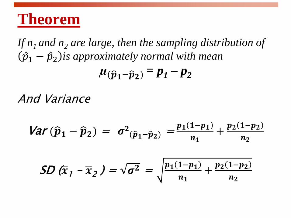
Theorem

If n1 and n2 are large, then the sampling distribution of

Ƹ𝑝1 − Ƹ𝑝2 is approximately normal with mean

µ(ෝ𝒑𝟏−ෝ𝒑𝟐) = p1 – p2

And Variance

Var (ෝ𝒑𝟏 − ෝ𝒑𝟐) = 𝝈𝟐(ෝ𝒑𝟏−ෝ𝒑𝟐) =𝒑𝟏 𝟏−𝒑𝟏

𝒏𝟏+

𝒑𝟐 𝟏−𝒑𝟐

𝒏𝟐

SD (ഥ𝒙1 – ഥ𝒙2 ) = 𝝈𝟐 = 𝒑𝟏 𝟏−𝒑𝟏

𝒏𝟏+

𝒑𝟐 𝟏−𝒑𝟐

𝒏𝟐

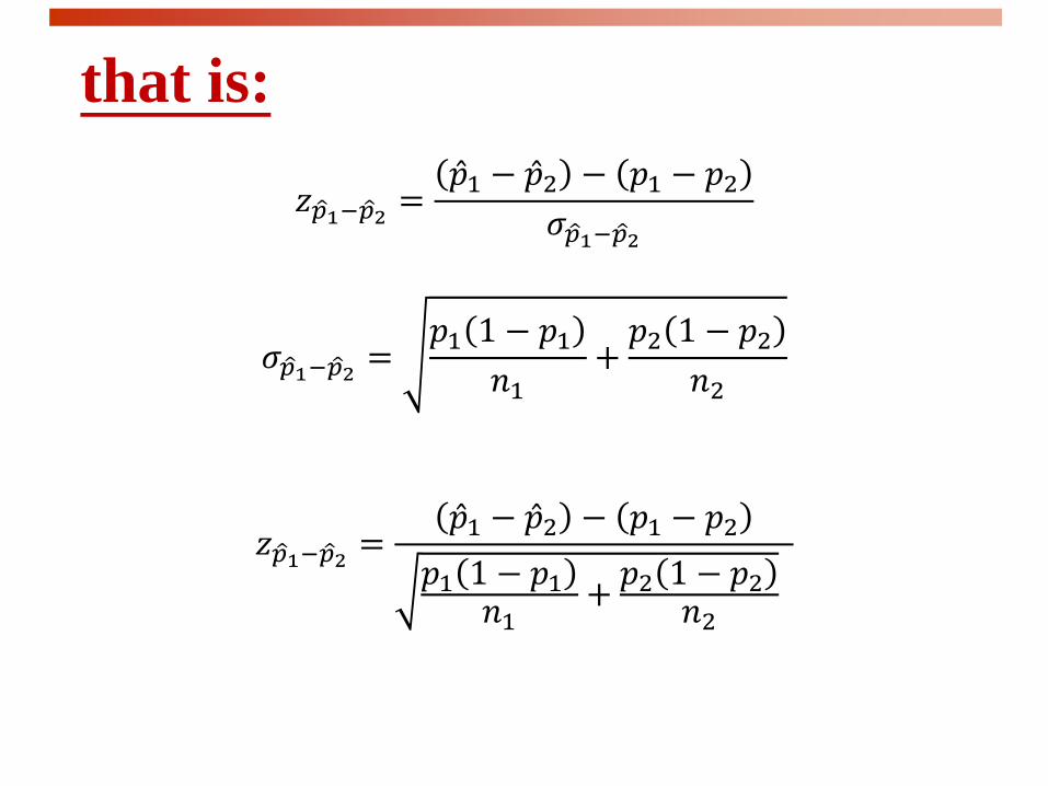
𝑧 ො𝑝1− ො𝑝2 =Ƹ𝑝1 − Ƹ𝑝2 − 𝑝1 − 𝑝2

𝜎 ො𝑝1− ො𝑝2

𝜎 ො𝑝1− ො𝑝2 =𝑝1 1 − 𝑝1

𝑛1+𝑝2 1 − 𝑝2

𝑛2

𝑧 ො𝑝1− ො𝑝2 =Ƹ𝑝1 − Ƹ𝑝2 − 𝑝1 − 𝑝2

𝑝1 1 − 𝑝1𝑛1

+𝑝2 1 − 𝑝2

𝑛2

that is:

Researchers found that among U.S. adults ages 75 or

older, 34 percent had lost all their natural teeth and for

U.S. adults ages 65-74, 26 percent had lost all their

natural teeth. Assume these properties are parameters

for the United States in those age groups. If a random

sample of 200 adults ages 65-74 and an independent

random sample of 250 adults ages 75 or older are

drawn from these populations, find the probability that

the difference in percent of total natural teeth loss is

less than 5 percent between the two population.

Example 4:

Solution

𝑝1 = .34 𝑛1 = 250 Ƹ𝑝1 − Ƹ𝑝2 = 0.05

𝑝2 = .26 𝑛2 = 200

𝜇 ො𝑝1− ො𝑝2 = 𝑝1 − 𝑝2= .34 − 26= 0.08

𝜎 ො𝑝1− ො𝑝2 =𝑝1 1 − 𝑝1

𝑛1+𝑝2 1 − 𝑝2

𝑛2

=0.34 0.66

250+

0.26 0.74

200

= 0.0431

𝑧 ො𝑝1− ො𝑝2 =Ƹ𝑝1 − Ƹ𝑝2 − 𝑝1 − 𝑝2

𝜎 ො𝑝1− ො𝑝2

=0.05 − 0.08

0.0431= −0.7

𝑃( Ƹ𝑝1 − Ƹ𝑝2 < 0.05) = 𝑃(𝑧 ො𝑝 < −0.7)

= 𝟎. 𝟐𝟒𝟐𝟎

𝑧 ො𝑝1− ො𝑝2 =Ƹ𝑝1 − Ƹ𝑝2 − 𝑝1 − 𝑝2

𝜎 ො𝑝1− ො𝑝2

𝜎 ො𝑝1− ො𝑝2 =𝑝1 1 − 𝑝1

𝑛1+𝑝2 1 − 𝑝2

𝑛2