Sampled Traffic Analysis byInternet-Exchange-Level Adversaries

Steven J. Murdoch and Piotr Zielinski

University of Cambridge, Computer Laboratoryhttp://www.cl.cam.ac.uk/users/{sjm217, pz215}

Abstract. Existing low-latency anonymity networks are vulnerable totraffic analysis, so location diversity of nodes is essential to defend againstattacks. Previous work has shown that simply ensuring geographical di-versity of nodes does not resist, and in some cases exacerbates, the risk oftraffic analysis by ISPs. Ensuring high autonomous-system (AS) diver-sity can resist this weakness. However, ISPs commonly connect to manyother ISPs in a single location, known as an Internet eXchange (IX). Thispaper shows that IXes are a single point where traffic analysis can beperformed. We examine to what extent this is true, through a case studyof Tor nodes in the UK. Also, some IXes sample packets flowing throughthem for performance analysis reasons, and this data could be exploitedto de-anonymize traffic. We then develop and evaluate Bayesian trafficanalysis techniques capable of processing this sampled data.

1 Introduction

Anonymity networks may be split into two categories: high latency (e.g. Mixmin-ion [1] and Mixmaster [2]) and low latency (e.g. Tor [3], JAP [4] and Free-dom [5]). High latency networks may delay messages for several days [6] butare designed to resist very powerful attackers which are assumed to be capa-ble of monitoring all communication links, so called global passive adversaries.However, the long potential delay makes these systems inappropriate for pop-ular activities such as web-browsing, where low-latency is required. Although,in low-latency anonymity networks, communications are encrypted to maintainbitwise-unlinkability, timing patterns are hardly distorted, allowing an attackerto deploy traffic analysis to de-anonymize users [7,8,9]. While techniques to resisttraffic analysis have been proposed, such as link padding [10], their cost is highand they have not been incorporated into deployed networks.

Instead, these systems have relied on the assumption that the global passiveadversary is unrealistic, or at least those who are the target of such adversarieshave larger problems than anonymous Internet access. But even excluding theglobal passive adversary, the possibility of partial adversaries remains reason-able. These attackers have the ability to monitor a portion of Internet traffic butnot the entirety. Distributed low-latency anonymity systems, such as Tor, aimto resist this type of adversary by distributing nodes, in the hope that connec-tions through the network will pass through enough administrative domains toprevent a single entity from tracking users.

N. Borisov and P. Golle (Eds.): PET 2007, LNCS 4776, pp. 167–183, 2007.

This raises the question of how to select paths through the anonymity net-work to maximize traffic analysis resistance. Section 2 discusses different topol-ogy models of the Internet and their impact on path selection. We suggest thatexisting models, based on Autonomous System (AS) diversity, do not properlytake account of the fact that while, at the AS level abstraction, a path mayhave good administrative domain diversity, physically it could repeatedly passthrough the same Internet eXchange (IX). Section 3 establishes, based on In-ternet topology measurements, to what extent the Tor anonymity network isvulnerable to traffic analysis at IXes.

Section 4 describes how IXes are particularly relevant since, to assist loadmanagement, they record traffic data from the packets being sent through them.As aggregate statistics are required and the cost of recording full traffic would beprohibitive, only sampled data is stored. Hence, the quality of data is substan-tially poorer than was envisaged during the design and evaluation of previoustraffic analysis techniques. Section 5 shows that, despite low sampling rates, thisdata is adequate for de-anonymizing users of low-latency anonymity networks.Finally, Section 6 discusses further avenues of research under investigation.

2 Location Diversity in Anonymity Networks

Tor has been long suspected, and later confirmed [11,12], to be vulnerable toan attacker who could observe both the entry and exit point of a connectionthrough an anonymity network. As no intentional latency is introduced, timingpatterns propagate through the network and may be used to correlate input andoutput traffic, allowing an attacker to track connection endpoints.

Delaying messages, as done with email anonymity systems, would improveresistance to these attacks, at least for a small number of messages. However,the additional latency here (hours to days) would, if applied to web browsing,deter most users and so decrease anonymity for the remainder [13]. In additionto the scarce bandwidth in a volunteer network, full link-padding would alsointroduce catastrophic denial of service vulnerabilities, because all parties wouldneed to stop communicating and re-negotiate flow levels when one party left.Hence, the only remaining defense against traffic analysis is to ensure that theadversary considered in the system threat model is not capable of simultaneouslymonitoring enough points in the network to break users’ anonymity.

While this approach would be of no help against a global passive adversary,more realistic attackers’ traffic monitoring capabilities are likely to be limited toparticular jurisdiction(s), whether they derive from legal or extra-legal powers.This intuitively leads to the idea that paths through anonymity networks shouldbe selected to go through as many different countries as possible. The hope hereis that an attacker attempting to track connections might have the ability tomonitor traffic in some countries, but not all those on the path.

Unfortunately, Feamster and Dingledine [14] showed this approach couldactually hurt anonymity because international connections were likely to gothrough one of a very small number of tier-1 Internet Service Providers (ISP) –

.se.cn

.au

.us

.br

AS1

AS2

IX

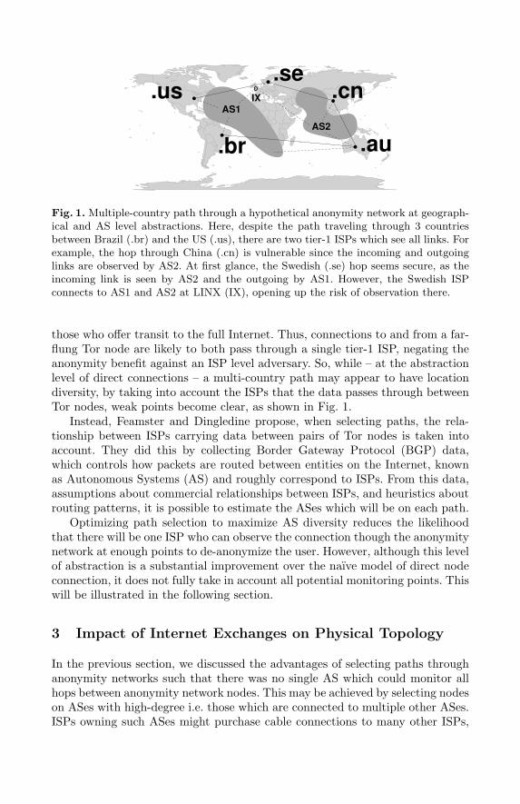
Fig. 1. Multiple-country path through a hypothetical anonymity network at geograph-ical and AS level abstractions. Here, despite the path traveling through 3 countriesbetween Brazil (.br) and the US (.us), there are two tier-1 ISPs which see all links. Forexample, the hop through China (.cn) is vulnerable since the incoming and outgoinglinks are observed by AS2. At first glance, the Swedish (.se) hop seems secure, as theincoming link is seen by AS2 and the outgoing by AS1. However, the Swedish ISPconnects to AS1 and AS2 at LINX (IX), opening up the risk of observation there.

those who offer transit to the full Internet. Thus, connections to and from a far-flung Tor node are likely to both pass through a single tier-1 ISP, negating theanonymity benefit against an ISP level adversary. So, while – at the abstractionlevel of direct connections – a multi-country path may appear to have locationdiversity, by taking into account the ISPs that the data passes through betweenTor nodes, weak points become clear, as shown in Fig. 1.

Instead, Feamster and Dingledine propose, when selecting paths, the rela-tionship between ISPs carrying data between pairs of Tor nodes is taken intoaccount. They did this by collecting Border Gateway Protocol (BGP) data,which controls how packets are routed between entities on the Internet, knownas Autonomous Systems (AS) and roughly correspond to ISPs. From this data,assumptions about commercial relationships between ISPs, and heuristics aboutrouting patterns, it is possible to estimate the ASes which will be on each path.

Optimizing path selection to maximize AS diversity reduces the likelihoodthat there will be one ISP who can observe the connection though the anonymitynetwork at enough points to de-anonymize the user. However, although this levelof abstraction is a substantial improvement over the naıve model of direct nodeconnection, it does not fully take in account all potential monitoring points. Thiswill be illustrated in the following section.

3 Impact of Internet Exchanges on Physical Topology

In the previous section, we discussed the advantages of selecting paths throughanonymity networks such that there was no single AS which could monitor allhops between anonymity network nodes. This may be achieved by selecting nodeson ASes with high-degree i.e. those which are connected to multiple other ASes.ISPs owning such ASes might purchase cable connections to many other ISPs,

but doing so would be extremely expensive. Instead, ISPs may connect theirnetwork to an IX, which will provide connectivity to all other ISPs with a pres-ence at that IX. This approach is more prevalent in Europe than in the US, dueto differing commercial structures and historical development; also because oflanguage differences, intra-country traffic is substantial.

Thus, while at the AS level it appears that the path makes multiple tran-sitions between distinct ASes, physically, each of these connections might passthrough the same IX. Hence, despite the path attaining high AS diversity, thereremains one entity who is able to de-anonymize the traffic. In order to establishhow much of a problem this is for deployed anonymity networks, we set out todetermine how successful an IX level adversary would be, compared to an ASlevel one, in de-anonymizing Tor users.

The techniques of Feamster and Dingledine [14] rely on building a map of ASpaths from BGP data, but this is not helpful for our purposes as the IXes do notappear at this level. From the perspective of a router in an IX, packets traveldirectly to the destination AS. Furthermore, their approach depends on informa-tion about ISP relationships and routing policies which are a carefully guardedsecret and so must be guessed. However, it is common practice to allocate eachrouter in an IX an IP address from a single subnet.

Hence, while the AS path of a connection will not reveal whether it is goingthrough an IX, a traceroute [15] is likely to. Unlike finding AS paths, collectingtraceroute data requires access to the system at both ends of the path. As Tordoes not currently implement a mechanism for performing traceroutes, theoperator of the node must do so manually. To limit the effort to a feasible level,here we take the UK as a case study.

3.1 Experimental Results

Based on geo-location databases and manual investigation, we identified Tornodes hosted in the UK and contacted the operators to request that they runa script to collect data to validate our hypothesis. One of our constraints wasthat no custom binary applications could be used, as the recipient could noteasily confirm they were benign. Instead, we simply invoked the OS providedtraceroute (or on Windows, tracert). These are not designed with speed orparallelism in mind, so to keep the runtime reasonable (2–24 hours, depending ontimeouts) on the slower Windows test machines we only traced 140 destinations,and on *nix machines, tested 595 destinations. These destinations consisted ofthe same 15 websites and 11 US consumer ISPs tested in [14] and the remainderwere randomly selected Tor nodes.

We received 19 (14 *nix, 5 Windows) responses from the 33 operators wewere able to contact. This totaled 9 025 paths with an average path length of 14hops (excluding failed responses). For each hop we established whether it was inone of the subnets of LINX (London InterNet eXchange), AMS-IX (AMSterdamInternet eXchange) or DE-CIX (the German Internet exchange, in Frankfurt).Also, using the Team Cymru Database [16], we established the BGP origin ASfor each IP address. Note that although we are arranging data by AS, this path

Table 1. Number of paths passing through ASes and IXes.

AS name (ASN) Paths %

Level 3 (3356) 1 961 22%NTL (5089) 1 445 16%Zen (13037) 1 258 14%JANET (786) 1 224 14%Datahop (6908) 996 11%Tiscali (3257) 953 11%Sprint (1239) 935 10%Cogent (174) 871 10%Telewest (5462) 698 8%Telia (1299) 697 8%

IX name (subnet) Paths %

LINX (195.66.224.0/22) 2 392 27%DE-CIX (80.81.192.0/22) 231 3%AMS-IX (195.69.144.0/22) 202 2%

is not the same as the BGP path discussed in [14]. Importantly, while IXes mayhave an AS, they do not broadcast routes, and so do not appear in BGP paths,whereas traceroute establishes the IP address of the border routers, from whichthe IX can be inferred.

The results are summarized in Table 1. As can be seen, Level 3, a largetier-1 ISP appears at least once on 22% of paths and other tier-1 ISPs, suchas Tiscali, Sprint, Cogent and Telia also appear. Since our tests were all fromUK Tor nodes, mainly run by volunteers, consumer ISPs also feature, such asNTL, Zen and Telewest, as does the UK academic network operator, JANET.Finally, Datahop, who provide connectivity between 10 data-centers in London,are present on 11% of paths. This broadly matches the results of [14], in that asmall number of ISPs are present many paths.

However, if we now examine whether an IX is on the path, we find a new classof observation points. Despite being invisible at the BGP level, LINX is presenton 27% of paths. There are 22 distinct ASes in the previous hop to LINX and109 following the LINX hop, so AS-diverse paths will not substantially impactLINX crossings. Hence, exploiting the IX as an observation point is an effectiveattack against both existing and proposed anonymity network routing schemes.The connectivity graph of selected ASes, based on our data, is shown in Fig. 2.

4 Traffic Analysis from Sampled Data

The previous section has shown how an adversary positioned at an IX would becapable of monitoring a substantial quantity of traffic through the Tor network.A powerful adversary would be in a position to install expensive hardware tomount conventional traffic analysis attacks but such an adversary would likely beable to deploy other, more effective, attacks. However, the network infrastructureprovided by an IX may already have the traffic analysis capabilities that a moremodest attacker could use.

NTL

Source

Level 3Zen

Cogent

JANET Telia

Telewest

Sprint

Tiscali

DatahopDestination

Fig. 2. AS connectivity via IX graph. Only ASes in Table 1 are shown and all sourcesand destinations are collapsed to single nodes. Links between ASes which pass throughLINX are shown as solid lines, AMS-IX is shown by dotted lines and DE-CIX bydashed lines. Paths which go through none of these IXes are omitted. From this wecan see that, in our data, connections through Sprint and Datahop go from source todestination without passing through any of the IXes we have selected.

To aid network management, high-end switches and routers have monitoringfeatures which, although not designed for this purpose, may still be effective intracing users of anonymity networks. This section will evaluate the suitability ofnetwork monitoring data for traffic analysis.

4.1 Traffic Monitoring in High-Speed Networks

On low-bandwidth small-office or business networks, full packet analysis toolssuch as tcpdump [17] are adequate to monitor traffic for debugging or to measureload. However, on links found on high-speed networks, the capacity required tostore all packets rapidly becomes infeasible. For example, at time of writing, bothLINX and AMS-IX carry approximately 150 Gb/s, which exceeds the theoreticalmaximum capacity of the high-speed PCIe bus, 64 Gb/s (32 lanes at 2 Gb/seach). Despite these difficulties, there is high demand for monitoring of suchhigh-speed links, to detect problems such as routing loops, balance load acrossnetwork infrastructure and anticipate future demands on capacity.

These applications do not rely on packet content, and for privacy reasons itmay be desirable not to record this at all. Thus, medium to high-end networkingequipment is commonly equipped with the ability to record aggregate data onthe traffic passing through it. One such mechanism is NetFlow [18], developedby Cisco Systems but supported by other equipment manufacturers. NetFlowequipped infrastructure records unidirectional flows as defined by a tuple (sourceIP, destination IP, source port, destination port, IP protocol, interface, class ofservice). For each of these, the device will record information such as the numberof packets, total byte count and bitwise-or of TCP flags.

A disadvantage of this approach is that it requires the network hardware toinspect every packet flowing through it. This can incur substantial load at highernetwork speeds, so to counter this difficulty sampled NetFlow only inspects aproportion q of packets. While sampling reduces CPU load, the network hard-ware must still store state for every flow it considers to be live, which couldpotentially be very large. An alternative, as adopted by sFlow [19], is to movethe aggregation out of the network device by immediately exporting sampledpacket headers. This approach also gives access to additional fields in packetheaders, such as the sequence number, which could be useful for traffic analy-sis. However, to ensure generality, we will concentrate on information availablein sampled NetFlow style data, which could be constructed from sFlow logs ifneeded (the converse is not true).

Not only is high-speed traffic monitoring possible with standard networkingequipment, but it is common practice to do so. Two examples which are particu-larly relevant to this paper are that AMS-IX record data for traffic managementmonitoring [20] and LINX (who record 1 in 2 048 packets [21]) additionally areconsidering using sFlow data for detecting email spam [22]. The same data couldalso assist tracking users of an anonymity network because Section 3.1 showedthat a significant number of Tor flows pass through an IX. In the followingsection we will examine how successful this type of traffic analysis would be.

4.2 Traffic Analysis Assumptions

There are two basic types of traffic analysis. The first treats the anonymitynetwork as a “black-box” and only inspects traffic entering and leaving the net-work. The second approach additionally examines flows within the network, andso improves the accuracy of the attack. In this paper, we will concentrate on theformer category. As this does not make any assumptions about the structure ofthe network, it is the more general approach. However, the techniques we presenthere could also be applied to the latter category of attacks, as intra-network Tortraffic will also often cross a small number of Internet exchanges.

We assume that the attacked flow passes through an attacker controlled IXon both its path into and out of the anonymity network. This would be thecase if, for example, both the customer and site are hosted on ISPs whose back-bone connection was through an IX under surveillance. Also, we assume thatpacket sampling is independently and identically distributed over the flow. Al-though some models of network hardware implement periodic sampling, ratherthan random, this assumption will remain true because Tor traffic makes up aninsignificant proportion of overall traffic.

The attacker observes a single flow going into the network and wishes toestablish which of several outgoing flows it corresponds to. This could be, forexample, finding which website a known criminal is uploading stolen data to.Alternatively, the attacker might wish to discover who has uploaded a particularvideo to a news website – now there is one outgoing flow and many incomingcandidates. In both cases, the attacker will have a number of candidates in mindwho are also generating traffic at the same time, and for our simulation we

assume that these produce around 1 000 flows per hour. We also assume thatthe adversary can distinguish Tor traffic from other traffic, which may triviallydone by IP address and port number, based on information in the Tor directory.

5 Mathematical Analysis

5.1 Model

Our model consists of n client-server flows. Each flow p = p1, . . . , pm is a col-lection of packets sent at times t1, . . . , tm. We model the times as a Poissonprocess with a start time s, duration l, and rate r (average packets per second).These three parameters are chosen independently at random for each flow.

Neither s, l, r nor the flow p are directly observable. The attacker sees adown-sampled version of p, in which each packet is retained independently witha fixed probability q, called a sampling rate (typically about 1/2 000). Each flowis sampled at the input and at the output, resulting in two vectors of times: xand y. Given a flow p, the sampling processes p→ x and p→ y are independent:

s, l, rPoisson−→ p x

sampling←− psampling−→ y (1)

In an n-flow system, the attacker sees all n output vectors y1, . . . , yn, andone input vector x, which corresponds to some yk. The task of the attacker isto compute the probability P (Tk) that x corresponds to yk, for each k.

To simplify the model, we assume that no packet from p appears simultane-ously in both x and y. Since x and y are independently sampled from p, a givenpacket from p appears in both x and y with the probability of q2 = 2.5 · 10−7,that is, once every 1/q2 = 4·106 packets (≈ 2 GB). Seeing the same packet on theinput and the output is thus very unlikely, which prevents packet-matching at-tacks [9] and makes independent random delays of individual packets practicallyunobservable in the sampled data. For simplicity, we therefore assume instanta-neous packet transmission. Section 5.5 shows that introducing a moderate delayto the system does not change the effectiveness of our attack.

The assumption of no common packets in x and y allows us to simplify (1)by observing that x and y are now independent Poisson processes with rate rq.

xPoisson←− s, l, rq

Poisson−→ y (2)

This simplification eliminates the original (unobservable) flow p from the model.

5.2 Basic Solution

Let Tk denote the event in which input x and output yk belong to the sameflow. In our model, the exact probabilities P (Tk) can be uniquely determinedfrom Bayes’ formula:

P (Tk|y1..n,x) =P (y1..n|Tk,x)P (Tk|x)∑i P (y1..n|Ti,x)P (Ti|x)

. (3)

Probabilities P (Tk|x) express our prior information about the target, possiblybased on the sampled input flow x (but not output flow y). For example, wemight know that a particular server k is just more popular than others, or thatit is the only one to regularly receive high-volume traffic and x looks to be high-volume. For simplicity, in the rest of the analysis, we treat all servers equally;any prior information can be easily taken into account using (3).

The probabilities P (y1..n|x, Tk) in (3) can be computed as follows:

P (y1..n|x, Tk) = P (yk|x, Tk)∏i 6=k

P (yi) =P (yk|x, Tk)

P (yk)

∏i

P (yi). (4)

Here, we used the fact that output flows yi are independent, and that P (yi|Tk) =P (yi): the information about input-output connection Tk is only relevant forstatements that involve both inputs and outputs (such as P (yk,x|Tk)).

Since we are only interested in relative probabilities for different k’s, we canignore all factors independent of k, such as P (x|Tk) = P (x) or

∏i P (yi), as they

would cancel out in (3) anyway:

P (Tk|y1..n,x)(3)∼ P (y1..n|x, Tk)

(4)∼ P (yk|x, Tk)P (yk)

=P (yk,x|Tk)

P (x|Tk)P (yk)∼ P (x,yk|Tk)

P (yk).

(5)We therefore need to compute P (yk) and P (x,yk|Tk). We are dealing with

a single flow x ← p → yk, so – to avoid notational clutter – we will drop theexplicit index k and assumption Tk from our formulae. In the new notation, wehave P (y) and P (x,y), which can be computed from appropriate conditionalprobabilities by integrating out the unknown parameters s, l, r:

P (y) =∫

s,l,r

P (y|s, l, r)P (s, l, r). (6)

P (x,y) =∫

s,l,r

P (x,y|s, l, r)P (s, l, r) =∫

s,l,r

P (x|s, l, r)P (y|s, l, r)P (s, l, r). (7)

The last equality holds because x and y, generated by model (2), are independentgiven s, l, r. The distribution P (s, l, r) expresses our prior knowledge about flowstarting times, durations, and rates.

We divide the interval [s, s + l] into infinitesimally small windows of size dt.Since y is a Poisson process (2), the probability of observing a single packet inone such window is rq dt. The probability of no packets in [s, s+ l] is e−rql. Thus,

P (y|s, l, r) =

{e−rql(rq dt)ny if all times in y ∈ [s, s + l],0 otherwise.

(8)

Here, ny is the number of packets in y. The same formula (with nx) holds forP (x|s, l, r). Since P (x,y|s, l, r) = P (x|s, l, r)P (y|s, l, r), we also have

P (x,y|s, l, r) =

{e−2rql(rq dt)nx+ny if all times in x,y ∈ [s, s + l],0 otherwise.

(9)

5.3 Long-Lived Flows

We first consider a simplified model, in which all flows start at the same knowntime s and have the same known duration l (basically, [s, s+ l] is our observationwindow). The only factor distinguishing the flows is their (unknown) rate r.From (8), we get:

P (y) =∫

r

P (y|r)P (r) =∫

r

e−rql(rq dt)nyP (r). (10)

where P (r) is our prior information about the rate r. Since r is a positive param-eter, we express our complete lack of prior knowledge by using the scale-invariantJeffrey’s ignorance prior P (r) ∼ r−1 dr [23]. This basically says that log r is dis-tributed uniformly: the probability of r ∈ [a, b] is proportional to log(b/a). Forexample, r ∈ [1, 10] and r ∈ [10, 100] have the same probability.

P (y)(10)=

∫r

(rq dt)nye−rqlP (r) = (q dt)ny

∫ ∞

r=0

rny−1e−rql dr =dtny

lnyΓ (ny).

(11)We used

∫∞0

za−1e−bz dz = Γ (a)/ba; for integer n we have Γ (n) = (n− 1)!.Similarly, from (9),

P (x,y) =∫

r

(rq dt)nx+nye−2rqlP (r) =dtnx+ny

(2l)nx+nyΓ (nx + ny). (12)

We can now use (5) to compute the final probability:

P (Tk|y1..n,x) ∼ P (x,yk|Tk)P (yk)

=dtnx

(2l)nx· Γ (nx + nyk

)2nyk Γ (nyk

)∼ Γ (nx + nyk

)2nyk Γ (nyk

). (13)

Interpretation. Fig. 3(a) shows a normalized plot of (13) for nx = 5 as afunction of ny. The maximum probability is assigned to ny ≈ nx, when thenumbers of observed packets on the input and on the output are similar. Thisconfirms our intuition and also yields quantitative probabilities for different ny’s,which can be used for combining evidence from multiple observations.

The exact maximum occurs for ny > nx because the prior P (r) ∼ r−1 drcauses P (r ∈ [4, 5]) > P (r ∈ [5, 6]) (because 5

4 > 65 ). This makes small ny’s more

probable to be produced by chance than larger ones, decreasing their matchprobability. Using Stirling’s approximation of n!, we get (see appendix):

P (Tk|y1..n,x) ∼ (nx + ny − 1)nx+ny− 12

2ny (ny − 1)ny− 12

, (14)

which very closely matches the original, as shown in Fig. 3(a). The maximum of(14), obtained by comparing its derivative to zero, is ny ≈ nx + 1

2 .

ny

P( T

k | x

, y1.

.n )

0 2 4 6 8 10 12 14

0

real (13)approx (14)

(a) P (Tk|x, y1..n) given by (13) for fixednx = 5 and ny ranging from 0 to 15.

miny

max

y

−25 −20 −15 −10 −5 0 5 10 15

−5

05

1015

2025

3035

(18)

(b) log P (Tk|x, y1..n) given by (18) fornx = ny = 5, min x = 0, max x = 10,and variable min y and max y.

Fig. 3. Relative probabilities based on (a) observed packet counts and (b) lengths.

5.4 General Flows

Now, we consider the general case, in which flows have different (unknown) du-rations l and starting times s. From (8), we can compute P (y|l, r) by integratings out. For a given duration l, the possible starting times s belong to the interval[max y − l, miny]. If ly = max y −miny is the observed length of y, then thisinterval of possible values of s has the length (l−ly)0 = max{l−ly, 0}. Assuminglack of prior knowledge about s (uniform prior P (s) ∼ ds), we have

P (y|l, r) =∫

s

P (y|s, l, r)P (s)(8)∼ (l − ly)0e−rql(rq dt)ny . (15)

Using Jeffrey’s priors P (l) ∼ l−1 dl and P (r) ∼ r−1 dr, we get:

P (y) =∫

l,r

P (y|l, r)P (l, r) =∫

l,r

(l − ly)0e−rql(rq dt)ny l−1r−1 dr dl =

(q dt)ny

∫l

(l − ly)0l−1

∫r

e−rqlrny−1 dr dl =

(q dt)ny

∫l

(l − ly)0l−1Γ (ny)(ql)−ny dl =

dtnyΓ (ny)∫ ∞

l=ly

(l − ly)l−ny−1 dl = dtnyΓ (ny)l−ny+1y

ny(ny − 1). (16)

We can compute P (x,y) in a similar way. Let nxy = nx + ny be the totalnumber of packets in x and y, and lxy = max{max x,max y}−min{minx,miny}

the observed length of superimposed sequences x and y. In general, lxy 6= lx+ly.

P (x,y) =∫

l,r

(l − lxy)0e−2rql(rq dt)nxy l−1r−1 dr dl =

Γ (nxy) dtnxy

2nxy (nxy)(nxy − 1)lnxy−1xy

. (17)

Ignoring all factors independent of k, (5) gives us the final probability

P (Tk|x,y1..n) =P (x,yk|Tk)

P (yk)∼ Γ (nxyk

)2nxyk Γ (nyk

)· nyk

(nyk− 1)

nxyk(nxyk

− 1)· l

nyk−1

yk

lnxyk

−1xyk

. (18)

Interpretation. Formula (18) consists of three factors: (i) the rate formula(13), (ii) a rate-dependent correction ny(ny − 1)/(nxy(nxy − 1)), and (iii) thelength-dependent factor l

ny−1y /l

nxy−1xy , which is of the most interest to us here.

Consider matching an input flow with the observed starting time minx = 0,ending time max x = 10, and nx = 5 observed packets, against output flows ywith the same number of observed packets ny = 5. For various starting and end-ing times min y and maxy, Fig. 3(b) presents the matching likelihood assignedby (18) (since nx and ny are constant, so are the first two factors).

As expected, the maximum is attained when the observed starting and endingtimes of both flows coincide: minx = miny = 0 and maxx = maxy = 10. Eachcontour line consists of two parallel straight lines joined by two curves. The twostraight lines correspond to the observed input flow period completely containingthe observed output flow period, and vice versa.

Optimality. The derivation of (18) is strictly Bayesian, so – given the modelassumptions – the result is exact and uses all relevant information. Note that,despite the timings of all packets being available through x and y, formula (18)uses only the total packet counts (ny, nxy) and the observed lengths (ly, lxy).This shows that the exact timings of individual packets (used by timing-basedattacks) are irrelevant for the inference in our model.

5.5 Evaluation

To evaluate the effectiveness of our method in attacking an individual Tor node,we first collected real traffic distributions of observed flow rates and durations(Fig. 4). Then, we performed a number of simulations of a 120 min execution of anode. Flow durations (1–30 min) and rates (0.1–50 packets/s) were drawn fromthe log-uniform (P (z) ∼ z−1 dz) prior, consistent with Fig. 4. Starting timeswere selected uniformly from the interval [0, 120 min− l].

Our scoring method was “1” if the highest probability was assigned to thecorrect target, and “0” otherwise (if i > 1 targets shared the top probability,

50 100 200 500 1000 2000

0.02

0.10

0.50

2.00

10.0

050

.00

Flow duration (s)

Rat

e (p

acke

ts/s

)

Fig. 4. Distribution of observed rates and flow durations on a single Tor node. Onlyflows that completed the three-way TCP handshake, at least 1 minute long, and consistof at least 5 packets are shown. Flows are closed after being idle for 1 minute.

then the score was 1/i instead of 1). For each simulation, we applied the attackindependently to each input, and then averaged the results.

We varied the following parameters: the number of flows per hour (50–1 000),the sampling rate q (1/100–1/2 000), the mean network latency (0–10 min), andthe attack method. Our parameter ranges are consistent with their real values:our Tor node transmitted 479 flows/h on average, the average Tor network la-tency was 0.5 s, and the current typical sampling rate is 1/2 048, but may increasein the future. The results of our simulations are summarized in Fig. 5.

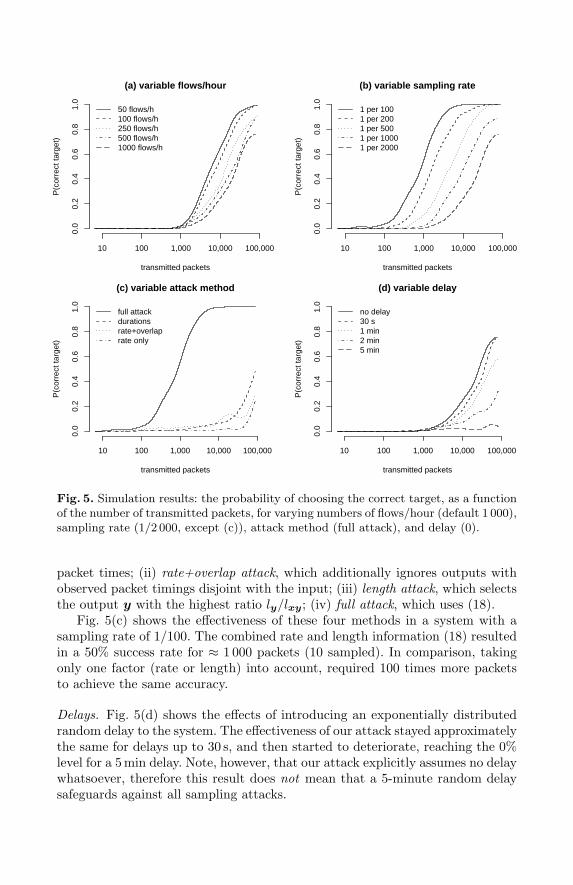
Average number of flows. Fig. 5(a) confirms that more flows provide more pro-tection. For a typical number of 500 flows/h, the attack had a 50% chance ofsuccess when the target sends ≈ 20 000 packets, that is ≈ 10 MB of data. With50 flows/h, the same success rate required only 7 000 packets (3.5 MB).

Sampling rate. Fig. 5(b) suggests that the effectiveness of the attack dependsonly on the number of sampled packets, so doubling the sampling rate is equiva-lent to doubling the number of transmitted packets. For the technically feasiblesampling rate of 1/100, a success rate of 50% required only 1 000 transmittedpackets (500 kB).

Attack methods. We compared the following attacks: (i) rate attack, which ap-plies (13), taking into account the observed number of packets and ignoring

0.0

0.2

0.4

0.6

0.8

1.0

(a) variable flows/hour

transmitted packets

P(c

orre

ct ta

rget

)

10 100 1,000 10,000 100,000

50 flows/h100 flows/h250 flows/h500 flows/h1000 flows/h

0.0

0.2

0.4

0.6

0.8

1.0

(b) variable sampling rate

transmitted packets

P(c

orre

ct ta

rget

)

10 100 1,000 10,000 100,000

1 per 100 1 per 2001 per 5001 per 10001 per 2000

0.0

0.2

0.4

0.6

0.8

1.0

(c) variable attack method

transmitted packets

P(c

orre

ct ta

rget

)

10 100 1,000 10,000 100,000

full attackdurationsrate+overlaprate only

0.0

0.2

0.4

0.6

0.8

1.0

(d) variable delay

transmitted packets

P(c

orre

ct ta

rget

)

10 100 1,000 10,000 100,000

no delay30 s1 min2 min5 min

Fig. 5. Simulation results: the probability of choosing the correct target, as a functionof the number of transmitted packets, for varying numbers of flows/hour (default 1 000),sampling rate (1/2 000, except (c)), attack method (full attack), and delay (0).

packet times; (ii) rate+overlap attack, which additionally ignores outputs withobserved packet timings disjoint with the input; (iii) length attack, which selectsthe output y with the highest ratio ly/lxy; (iv) full attack, which uses (18).

Fig. 5(c) shows the effectiveness of these four methods in a system with asampling rate of 1/100. The combined rate and length information (18) resultedin a 50% success rate for ≈ 1 000 packets (10 sampled). In comparison, takingonly one factor (rate or length) into account, required 100 times more packetsto achieve the same accuracy.

Delays. Fig. 5(d) shows the effects of introducing an exponentially distributedrandom delay to the system. The effectiveness of our attack stayed approximatelythe same for delays up to 30 s, and then started to deteriorate, reaching the 0%level for a 5 min delay. Note, however, that our attack explicitly assumes no delaywhatsoever, therefore this result does not mean that a 5-minute random delaysafeguards against all sampling attacks.

6 Future Work

For simplicity, we ignored several phenomena that occur in practice, such asdifferent sampling rates and how Tor cells are split over IP packets. Generalizingour analysis to support different known sampling rates at input and output seemsstraightforward (but an attack by a single adversary with a fixed sampling rateis most likely). Similarly, the effect of packet splitting by Tor nodes seems tobe statistically equivalent to different sampling rates. Our analysis could alsobe modified to take TCP sequence numbers, available from sFlow records, intoaccount, to give more accurate rate calculation.

As reasonable random delays do not protect against our attack, we plan toexamine other defenses, such as a moderate amount of dummy traffic. We wouldalso like to measure the effectiveness of our attack against real systems, usingan empirically determined prior distribution on durations and rates, for boththe analysis (numerical integration required) and the evaluation. Ideally, suchan evaluation should be performed for the entire Tor system, with its average1 million flows per hour.

Furthermore, we are considering how intra-network traffic analysis could beperformed. Similar techniques could be used, and are likely to work better thanwhole-network analysis since the number of flows will be smaller. However, thereare complications which must be considered, in particular that multiple flowsbetween the same pair of Tor nodes may be multiplexed within one encryptedTLS tunnel. An improved analysis would take this possibility into account andempirical studies would show to what extent this interferes with analysis.

7 Conclusion

We have demonstrated that Internet exchanges are a viable, and previouslyunexamined, monitoring point for traffic analysis purposes. They are present onmany paths through our sample of the Tor network, even where BGP data wouldnot detect any common points of failure. Furthermore, Internet exchanges areparticularly relevant as in some cases they may record, and potentially retaindata adequate to perform traffic analysis.

To validate to what extent this was true, we developed traffic analysis tech-niques which work on the sampled data which is being collected in practice byInternet exchanges. Using a Bayesian approach, we obtained the best possibleinference, which means that we can not only attack vulnerable systems, but alsodeclare others as safe under our threat model. Our probability formula is difficultto obtain by trial-and-error, and – as we show – can give orders of magnitudebetter results than simple intuitive schemes.

We also show that exact “internal” packet timings are irrelevant for optimuminference, so timing-based attacks cannot work with sparsely sampled data. Forthe same reason, deliberate random packet delays do not protect low-latencyanonymity systems against our attack, as the minimum sensible latency (1 min)is unacceptable for web browsing and similar activities.

Acknowledgments We thank Richard Clayton, Chris Hall, Markus Kuhn,Andrei Serjantov and the anonymous reviewers for productive comments, andalso the Tor node operators who collected the data used in this paper.

References

1. Danezis, G., Dingledine, R., Mathewson, N.: Mixminion: Design of a Type IIIAnonymous Remailer Protocol. In: Proceedings of the 2003 IEEE Symposium onSecurity and Privacy. (2003)

2. Moller, U., Cottrell, L., Palfrader, P., Sassaman, L.: Mixmaster Protocol – Version2. Draft (2003)

3. Dingledine, R., Mathewson, N., Syverson, P.: Tor: The second-generation onionrouter. In: Proceedings of the 13th USENIX Security Symposium. (2004)

4. Berthold, O., Federrath, H., Kopsell, S.: Web MIXes: A system for anonymousand unobservable Internet access. In Federrath, H., ed.: Proceedings of DesigningPrivacy Enhancing Technologies: Workshop on Design Issues in Anonymity andUnobservability, Springer-Verlag, LNCS 2009 (2000) 115–129

5. Boucher, P., Shostack, A., Goldberg, I.: Freedom systems 2.0 architecture. Whitepaper, Zero Knowledge Systems, Inc. (2000)

6. Serjantov, A., Murdoch, S.J.: Message splitting against the partial adversary. In:Proceedings of Privacy Enhancing Technologies workshop (PET 2005), Springer-Verlag, LNCS 3856 (2005)

7. Serjantov, A., Sewell, P.: Passive attack analysis for connection-based anonymitysystems. In: Proceedings of ESORICS 2003. (2003)

8. Levine, B.N., Reiter, M.K., Wang, C., Wright, M.K.: Timing attacks in low-latencymix-based systems. In Juels, A., ed.: Proceedings of Financial Cryptography (FC’04), Springer-Verlag, LNCS 3110 (2004)

9. Danezis, G.: The traffic analysis of continuous-time mixes. In: Proceedings ofPrivacy Enhancing Technologies workshop (PET 2004). Volume 3424 of LNCS.(2004)

10. Dai, W.: Pipenet 1.1. Post to Cypherpunks mailing list (1998) http://www.

eskimo.com/~weidai/pipenet.txt.11. Øverlier, L., Syverson, P.: Locating hidden servers. In: Proceedings of the 2006

IEEE Symposium on Security and Privacy, IEEE CS (2006)12. Bauer, K., McCoy, D., Grunwald, D., Kohno, T., Sicker, D.: Low-resource routing

attacks against anonymous systems. Technical Report CU-CS-1025-07, Universityof Colorado at Boulder (2007)

13. Acquisti, A., Dingledine, R., Syverson, P.: On the Economics of Anonymity.In Wright, R.N., ed.: Proceedings of Financial Cryptography (FC ’03), Springer-Verlag, LNCS 2742 (2003)

14. Feamster, N., Dingledine, R.: Location diversity in anonymity networks. In: Pro-ceedings of the Workshop on Privacy in the Electronic Society (WPES 2004),Washington, DC, USA (2004)

15. Jacobson, V.: traceroute (1) (1987) ftp://ftp.ee.lbl.gov/traceroute.tar.gz.16. Team Cymru: IP to ASN lookup (v1.0) http://asn.cymru.com/.17. Jacobson, V., Leres, C., McCanne, S.: tcpdump (1) (1989) http://www.tcpdump.

org/.18. Claise, B.: Cisco systems NetFlow services export version 9. RFC 3954, IETF

(2004)

19. Phaal, P., Panchen, S., McKee, N.: InMon corporation’s sFlow: A method formonitoring traffic in switched and routed networks. RFC 3176, IETF (2001)

20. Jasinska, E.: sFlow – I can feel your traffic. In: 23C3: 23rd Chaos Com-munication Congress. (2006) http://events.ccc.de/congress/2006/Fahrplan/

attachments/1137-sFlowPaper.pdf.21. Hughes, M.: LINX news. http://www.uknof.org.uk/uknof4/Hughes-LINX.pdf

(2006)22. Clayton, R.: spamHINTS project (2006) http://www.spamhints.org/.23. Jaynes, E.T.: Probability Theory: The Logic of Science. Cambridge University

Press (2003)

A Appendix

Theorem 1. Formula (13) attains maximum for ny ≈ nx + 12 .

Proof. Stirling’s factorial approximation gives us

n! ≈(n

e

)n√2πn.

Denoting a = nx, b = ny, and c = a + b, we have:

P (Tk|y1..n,x) ∼ Γ (a + b)2bΓ (b)

=(c− 1)!

2b(b− 1)!≈

(c−1

e

)c−1 √2π(c− 1)

2b(

b−1e

)b−1 √2π(b− 1)

∼

(c− 1)c− 12

2b(b− 1)b− 12

= X. (19)

Instead of finding the maximum of X, it is easier to find the maximum oflog X:

log X = (c− 12 ) log(c− 1)− b log 2− (b− 1

2 ) log(b− 1). (20)

We can find the maximum of log X by differentiating it w.r.t. b, and remem-bering that c′ = (a + b)′ = 1:

(log X)′ = log(c− 1) +c− 1

2

c− 1− log 2− log(b− 1)−

b− 12

b− 1

= log(c− 1) +1

2(c− 1)− log 2− log(b− 1)− 1

2(b− 1)

≈ log(c− 12 )− log 2− log(b− 1

2 ) = log(

c− 12

2b− 1

).

(21)

Now, (log X)′ = 0 implies c − 12 = 2b − 1, which implies b = a + 1

2 , that isny = nx + 1

2 .