S3+Perturbation+2011
22
Page 3.1 SECTION 3: STATIONARY-STATE PERTURBATION THEORY 1. Introduction 2 2. Perturbation of a non-degenerate level 3 2.1 First-order theory 4 2.2 Second-order theory 7 2.3 Condition on the strength of the perturbation 7 3. Perturbation of the harmonic oscillator 8 3.1 Reminder of the one-dimensional harmonic oscillator 8 3.2 Linear perturbation of a one-dimensional oscillator 9 4. Perturbation of a degenerate level 10 4.1 Statement of the problem 10 4.2 First-order theory 12 4.3 Diagonalization of the submatrix 13 4.4 Diagonalizing the submatrix using symmetry 14 5. The Stark Effect in Hydrogen 16 5.1 Reminder of the hydrogen atom 16 5.2 The Stark Effect: hydrogen in a uniform electric field 17 References The original version of these notes was based on sections 7.1 and 7.3 of the book by Mandl, with additional material from sections 6.1 and 6.2 of the textbook of Griffith. The section on the application to the Stark Effect is adapted from the textbooks by Gasiorowicz and Liboff; further details are given as footnotes where ap- propriate. Original Version: 1995; Last Major Revision: October 2002 Revision Date: 26 October 2010 Printed: 26 October 2010
-
Upload
lucas-mosimanegape-gailele -
Category
Documents
-
view
212 -
download
0
description
perturbation theoryquantum mechanics
Transcript of S3+Perturbation+2011

Page 3.1
SECTION 3: STATIONARY-STATE PERTURBATION THEORY
1. Introduction 2
2. Perturbation of a non-degenerate level 3
2.1 First-order theory 4
2.2 Second-order theory 7
2.3 Condition on the strength of the perturbation 7
3. Perturbation of the harmonic oscillator 8
3.1 Reminder of the one-dimensional harmonic oscillator 8
3.2 Linear perturbation of a one-dimensional oscillator 9
4. Perturbation of a degenerate level 10
4.1 Statement of the problem 10
4.2 First-order theory 12
4.3 Diagonalization of the submatrix 13
4.4 Diagonalizing the submatrix using symmetry 14
5. The Stark Effect in Hydrogen 16
5.1 Reminder of the hydrogen atom 16
5.2 The Stark Effect: hydrogen in a uniform electric field 17
References
The original version of these notes was based on sections 7.1 and 7.3 of the book by Mandl, with additional
material from sections 6.1 and 6.2 of the textbook of Griffith. The section on the application to the Stark Effect
is adapted from the textbooks by Gasiorowicz and Liboff; further details are given as footnotes where ap-
propriate.
Original Version: 1995; Last Major Revision: October 2002
Revision Date: 26 October 2010
Printed: 26 October 2010

Page 3.2
1. INTRODUCTION
As already mentioned in connection with the variational method, most physical problems of interest cannot
be solved exactly so approximate methods must be used.
• Perturbation theory is one such method; here we look at its application to bound-state problems (i.e.
problems which are essentially time independent)1.
• In contrast to the variational method, perturbation theory can be used to predict both the energy and
wave function of a quantum system.
• The method involves finding approximately the stationary states of a system which differs only slightly
from a system whose stationary states may be regarded as known.
• As an example, assuming that we know the stationary states of a particular atom, we can use perturbation
theory to determine the states of the atom when placed in a weak electric or magnetic field.
We wish to find the eigenstates Ψn, n = 1, 2, 3, ⋯ and corresponding energies En of a system with Hamiltonian
H, i.e. we want to solve the time-independent Schrödinger equation
n n nH EΨ = Ψ (1)
The label n = 1, 2, 3, ⋯ distinguishes the different eigenstates of the system in order of increasing energy. We
split the Hamiltonian of the system into two terms:
0H H V= + (2)
where
1) H0 is the unperturbed Hamiltonian of the system whose solution is known, and
2) V is a perturbation which is in some sense small (what this means is discussed later).
We assume that the energy spectra of both H and H0 are discrete (this is easily generalized2), with
( )00 n n nH EΦ = Φ . (3)
• The nΦ are the known orthonormal solutions of the unperturbed Hamiltonian H0, and
• The ( )0nE are the corresponding known energies of the unperturbed system.
To solve the physical problem we modify eq.(2):
0( )H H Vλ λ= + (4)
where we have introduced into eq.(2) a variable parameter λ, with
1 corresponding to the physical problem to be solved
0 corresponding to the already solved unperturbed problem.
λ
λ
=
=
We wish to know the effect of the perturbation λV on a particular solution ( )0,n nEΦ of the unperturbed
Hamiltonian.
1Such methods are also used in classical physics. Perturbation theory was introduced into quantum mechanics by Schrödinger (1926). 2See the brief discussion in the textbook by Mandl (in the middle of page 166).

Page 3.3
Fig.1 shows schematically a possible plot of the energy eigenstates of the Hamiltonian H(λ) as a function of
the perturbation strength λ. In this figure
• the state labelled 1 is non-degenerate;
• the states labelled 2 and 3 are degenerate and this degeneracy is removed when the perturbation is
included;
• the states labelled 4 and 5 are degenerate, and remain degenerate as the perturbation is added.
Figure 1: Schematic energy spectrum showing the effect of including a small perturbation
How we proceed depends on whether or not the particular unperturbed energy state under consideration is
degenerate, i.e. on whether more than one solution to the Schrödinger equation corresponds to a given energy
( )0nE .
2. PERTURBATION OF A NON-DEGENERATE LEVEL
We first discuss the case where the unperturbed state n under consideration is non-degenerate3; i.e. corre-
sponding to the unperturbed energy ( )0nE there is a single state nΦ . We must find the eigenvalue En and
corresponding eigenvector Ψn of the full Hamiltonian H, eq.(1):
n n nH EΨ = Ψ
The effect of the small perturbation λV is to modify slightly the state nΦ and its energy ( )0nE : nΦ will go
over into nΨ and ( )0nE will shift slightly to En. We therefore expand both En and nΨ in powers of the
modified perturbation λV and assume that both series converge.
(0) (1) 2 (2)
(1) 2 (2)
zero-order first-order second-order
n n n n
n n n n
E E E Eλ λ
λ λ
= + + +
Ψ = Φ + Φ + Φ +
↑ ↑ ↑
⋯
⋯ (5)
The first-order corrections are proportional to the perturbation V, the second-order corrections proportional
to 2V and so on.
3This discussion is based on section 7.1 of the textbook of Mandl. See also section 6.1 of the book of Griffith.

Page 3.4
The second expansion is not unique; the substitution (1) (1) (0)n n ncΦ → Φ + Φ , where c is an arbitrary constant,
leads to the same energy correction (1)nE . To make the expansion unique we can impose one of two constraints:
• We can insist that the corrections ( )inΦ to the wave function are all orthogonal to the unperturbed wave
function Φn:
(1) (2) 0n n n nΦ Φ = Φ Φ = =⋯ (6)
• As an alternative, we could insist that Ψn is already normalised to all orders of perturbation theory.
Both choices lead to the same energy corrections and to wave functions that differ at most by an overall phase
factor (the predictions for observables would therefore be unchanged). We follow the first choice and impose
constraint (6).
The expansions (5) are now substituted in the Schrödinger equation (1) together with the modified Ham-
iltonian (4) to give
( ) (1) (0) (1) (1)0 n n n n n nH V E Eλ λ λ λ + Φ + Φ + = + + Φ + Φ +
⋯ ⋯ ⋯ .
This equation must hold for all values of the parameter λ, i.e. the coefficients of each power of λ must vanish
separately. This leads to the infinite set of equations:
( ) ( )( ) ( )
0 (0)0
1 (0) (1) (1)0
2 (0) (2) (1) (1) (2)0
Coefficient of
Coefficient of
Coefficient of
n n n
n n n n
n n n n n n
H E
H E V E
H E V E E
λ
λ
λ
Φ = Φ
− Φ = − − Φ
− Φ = − − Φ + Φ
(7)
and so on.
• The first equation is simply the zero-order approximation to the full problem, for which the solution is
known.
• The second of the equations then gives the first-order corrections, (1)nE and (1)
nΦ .
• The next equation can then be solved to give the second-order corrections, and so on.
In principle, the original problem can therefore be solved to any order of perturbation theory. In practice,
however, the equations to be solved become more and more complicated for each successive order, and the
series may in any case start to diverge. If the solution to low order is not sufficiently accurate, then a different
method should be used.
2.1 First-order theory
The second of eqs.(7) gives the first-order corrections, (1)nE and (1)
nΦ , to the unperturbed energy and wave
function:
( ) ( )(0) (1) (1)0 n n n nH E V E− Φ = − − Φ
To determine the first-order correction to the energy, we take the scalar product of this equation with Φn, the
wave function of the unperturbed state, giving
(0) (1) (1)0n n n n n n n nH E V EΦ − Φ = − Φ Φ + Φ Φ (8)
Now
(0) (1) (1) (0) (1)0 0n n n n n n n nH E H EΦ − Φ = Φ Φ − Φ Φ

Page 3.5
From eq.(3),
(0)0n n nH EΦ = Φ
so that
(0) (1) (0) (1) (0) (1)0 0n n n n n n n n nH E E EΦ − Φ = Φ Φ − Φ Φ =
showing that the left-hand side of eq.(8) is identically zero.
The second term on the right-hand side of eq.(8) becomes (1)nE because of the orthonormality of the un-
perturbed states Φn:
(1) (1) (1)n n n n n n nE E EΦ Φ = Φ Φ =
Hence we get the simple result
(1)n n nE V= Φ Φ (9)
This is one of the most useful equations in quantum mechanics.
• It says that the main effect of the perturbation V is simply to shift the unperturbed energy by an amount
equal to the expectation value of the perturbation itself (with respect to the unperturbed state Φn). The
result does not depend in any way on any other state of the system.
Hence we have, to first order,
n n n n nE H H≡ Ψ Ψ Φ Φ≃
To find the first-order correction to the wave function, we return to the second of the eqs.(7) and take the
scalar product with the wave function of any other unperturbed state, i.e. with Φp for some p ≠ n,
(0) (1) (1)0p n n p n p n nH E V EΦ − Φ = − Φ Φ + Φ Φ .
The last term in the equation is identically zero because of the orthogonality of the states Φp and Φn:
(1) (1) 0p n n n p nE EΦ Φ = Φ Φ =
since p ≠ n
We define Vpn as the matrix element of the perturbation in the basis of unperturbed states:
pn p nV V≡ Φ Φ
After simplifying the left-hand side of the equation we have:
( )(0) (0) (1)p n p n pnE E V− Φ Φ = −
Thus a formal expression for the first-order correction to the wave function is:
( )
(1)
(0) (0)
pn
p n
p n
V
E E
−Φ Φ =
−; (10)
this gives the components of the correction in the basis of the unperturbed states. To make this more explicit
and to derive a more useful expression, we expand the correction (1)nΦ in the complete set Φq of eigenstates
of H0:
(1)n nq q
q
aΦ = Φ∑

Page 3.6
Now
(1)n n nq n q nq nq nn
q q
a a aδΦ Φ = Φ Φ = =∑ ∑
But (1) 0n nΦ Φ = according to eq.(6). Hence ann = 0 and the sum over q in the expansion for the correction
does not contain n:
(1)n nq q
q n
a≠
Φ = Φ∑ (11)
Similarly, for p ≠ n
(1)p n nq p q nq pq np
q n q
a a aδ≠
Φ Φ = Φ Φ = =∑ ∑
and eq.(10) becomes
( )(0) (0)
pn
np
p n
Va
E E
−=
−
Finally, from the expansion eq.(11)
(1)
(0) (0)
qnn q
q n n q
V
E E≠
Φ = Φ−∑ (12)
giving, to first order,
(1)
(0) (0)
qnn n n n q
q n n q
V
E E≠
Ψ = Φ + Φ = Φ + Φ−∑
• Note that the expression for the perturbed wave function Ψn of the n’th level contains components
proportional to all the eigenfunctions of the unperturbed Hamiltonian – the perturbation V mixes the
unperturbed state n with all the other unperturbed states q with q ≠ n.
• Obviously, because of the presence of the energy difference (0) (0)n qE E− in the denominator of each term,
neighbouring levels have the largest effect on the wave function, and distant levels will have relatively
little effect, at least individually.
Note also that the normalization of the approximate wave function is
(1) (1)
(1) (1) 2 (1) (1)
n n n n n n
n n n n n n n n
λ λ
λ λ λ
Ψ Ψ = Φ + Φ Φ + Φ
= Φ Φ + Φ Φ + Φ Φ + Φ Φ
But by assertion (6)
(1) (1) 0n n n n
∗Φ Φ = Φ Φ =
Therefore we have
21 ( )n n O λΨ Ψ = +
showing that, in fact, Ψn is correctly normalized to first order. This is not the case when higher-order cor-
rections to the wave function are included; then Ψn must be explicitly normalized.

Page 3.7
2.2 Second-order theory
The first-order correction to the energy is sometimes identically equal to zero (see the example on the
harmonic oscillator below). We must then calculate the second-order correction. Consider the third of the
eqs.(7),
( ) ( )(0) (2) (1) (1) (2)0 n n n n n nH E V E E− Φ = − − Φ + Φ (13)
Taking the scalar product with nΦ we get:
(0) (2) (1) (1) (2)0n n n n n n n n nH E V E EΦ − Φ = − Φ − Φ + Φ Φ .
After slight manipulation, this leads to
(2) (1)n n nE V= Φ Φ
or, finally, using eq.(12) and the fact that, since V is Hermitian, qn nqV V ∗= :
2
(2)
(0) (0)
nq
n
q n n q
VE
E E≠
=−∑ (14)
• Thus, the second-order correction to the energy depends on the wave functions of all unperturbed states
(recall that in first order, the energy correction for state n depends only on the unperturbed wave function
of state n).
• For the ground state, the denominator of each term in the sum is negative. Hence the energy correction
(2)nE must be negative.
• If an important state “q” (i.e. important in the sense of lying nearby, or of Vnq being large) lies above a
given level “n”, then the second-order shift is downwards; if it lies below it, the shift is upwards. This is
often referred to as the tendency of levels to repel one another.
An expression for the second-order correction to the wave function, if needed, can be found by taking the
scalar product of eq.(13) with Φp, p ≠ n. The result, which contains a double sum over all unperturbed states,
can be found in most textbooks on quantum mechanics. The calculation of higher-order terms is not usually
necessary.
2.3 Condition on the strength of the perturbation
For the energy and wave function corrections to be small compared to the zero-order terms we require, from
eqs.(12) and (14),
(0) (0) for all qn n qV E E q n− ≠≪ . (15)
Making the reasonable assumption that all off-diagonal matrix elements of the perturbation V are the same
order of magnitude, this means that we require
(0)(0) for all nq n nV E E q n′− ≠≪ (16)
where n′ labels the unperturbed state closest in energy to state n.
• These conditions ensure that the first-order corrections are small, and first-order theory is sufficient to
describe the system with reasonable accuracy.
• On the other hand, if the energy gap between the state n and the state closest in energy, n′, is small, then

Page 3.8
the condition eq.(16) breaks down and non-degenerate perturbation theory is not useful; the theory to be
developed below for degenerate states should be used instead.
3. PERTURBATION OF THE HARMONIC OSCILLATOR
Many physical systems approximate the harmonic oscillator provided the amplitude of the motion is suffi-
ciently small. A better approximation often results if potential energy terms linear, cubic (or even quartic) in
displacement are added to the usual quadratic potential energy term; the effect of these additional terms can
be computed using low-order perturbation theory.
Alternatively, an extra interaction term in the Hamiltonian may arise by, for example, placing the charged
particle in a magnetic or electric field. This extra term, which may be linear, cubic ... in displacement, can
again be treated using perturbation theory4.
3.1 Reminder of the one-dimensional harmonic oscillator5
The Hamiltonian of an oscillating particle of mass m is given by:
2
2 21
2 2
pH m x
mω= + (17)
where ω is the oscillator parameter. The eigenvalues of this Hamiltonian are:
(0) 1( ) for 0,1,2,
2nE n nω= + =ℏ ⋯ (18)
which are all non-degenerate, and the eigenvectors are denoted:
2 21( )exp( )
2n n nN H x xφ α α= − (19)
where 2 mωα =
ℏ. The normalization factor is
2
1/22 !n n
Nn
α
π=
and the first few Hermite polynomials are:
0
1
22
1
2
(2 ) 2
H
H x
H x
α
α
=
=
= −
⋮
and so on. The matrix elements of x in the basis of oscillator states can be expressed6 as:
4Perturbation of the linear harmonic oscillator by various perturbations is treated in Quantum Mechanics Volume 2, by C Cohen-Tannoudji, B Diu and F Laloë, published by Wiley, 1977. The discussion here is based on pages 1151-2 of this book (they also give the exact solution); see also problem 7.2 of the textbook by Mandl and problem 6.5 of the book by Griffith. 5 See section 2.7 of Mandl or section 2.3 of Griffith. 6 See problem 3.50 (1st edition) or 3.33 (2nd edition) of the textbook by Griffith.
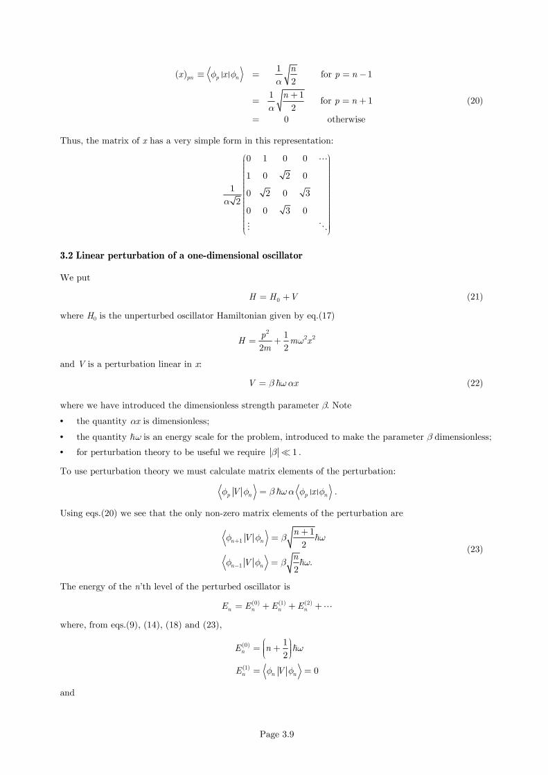
Page 3.9
1( ) for 1
2
1 1for 1
20 otherwise
pn p n
nx x p n
np n
φ φα
α
≡ = = −
+= = +
=
(20)
Thus, the matrix of x has a very simple form in this representation:
0 1 0 0
1 0 2 0
10 2 0 3
20 0 3 0
α
⋯
⋮ ⋱
3.2 Linear perturbation of a one-dimensional oscillator
We put
0H H V= + (21)
where H0 is the unperturbed oscillator Hamiltonian given by eq.(17)
22 21
2 2
pH m x
mω= +
and V is a perturbation linear in x:
V xβ ωα= ℏ (22)
where we have introduced the dimensionless strength parameter β. Note
• the quantity αx is dimensionless;
• the quantity ℏω is an energy scale for the problem, introduced to make the parameter β dimensionless;
• for perturbation theory to be useful we require 1β ≪ .
To use perturbation theory we must calculate matrix elements of the perturbation:
p n p nV xφ φ β ωα φ φ= ℏ .
Using eqs.(20) we see that the only non-zero matrix elements of the perturbation are
1
1
1
2
.2
n n
n n
nV
nV
φ φ β ω
φ φ β ω
+
−
+=
=
ℏ
ℏ
(23)
The energy of the n’th level of the perturbed oscillator is
(0) (1) (2)n n n nE E E E= + + +⋯
where, from eqs.(9), (14), (18) and (23),
(0)
(1)
1
2
0
n
n n n
E n
E V
ω
φ φ
= +
= =
ℏ
and

Page 3.10
2
(2)
(0) (0)
2 2
1 1
(0) (0) (0) (0)1 1
p n
n
p n n p
n n n n
n n n n
VE
E E
V V
E E E E
φ φ
φ φ φ φ
≠
+ −
+ −
=−
= +− −
∑
The values of the matrix elements are given in eqs.(23), and we also have
(0) (0)1
(0) (0)1
n n
n n
E E
E E
ω
ω
+
−
− = −
− = +
ℏ
ℏ
Substituting these values into the previous equation and rearranging yields
(2) 2 2 21 1 1( 1)
2 2 2nE n nβ ω β ω β ω=− + + = −ℏ ℏ ℏ
and finally
21 1
2 2nE n ω β ω
= + − + ℏ ℏ ⋯
Note that
• there is no shift in the oscillator energy to first order, and
• the second-order shift is the same for all energy levels.
In the same way, it is easily shown that to first order the wave function of the perturbed system is, from
eq.(12),
(0) (0)
1 1
1.
2 2
p n
n n n
p n n p
n n n
V
E E
n n
φ φψ φ φ
φ β φ β φ
≠
+ −
= +−
+= − +
∑
We see that the perturbation mixes each oscillator state only with its two neighbouring states; the amount of
configuration mixing is proportional to the strength of the perturbation.
4. PERTURBATION OF A DEGENERATE LEVEL
4.1 Statement of the problem
We now consider the situation where the state Φn of interest is degenerate7. The need for a modification to the
theory already developed is obvious from inspection of eq.(12), for example, where at least one term in the
expansion will be infinite if a second unperturbed state has the same energy as the state Φn. We will see below
how to circumvent this difficulty.
We assume that a particular eigenvalue (0)nE of H0 is N-fold degenerate, i.e. there are N linearly-independent
eigenvectors
7This discussion is based on section 7.3 of the textbook of Mandl (although the discussion here is greatly expanded). See also section 6.2 of the book of Griffith.

Page 3.11
( ) , 1,2, ,n Nα αΦ = … (24)
corresponding to the same unperturbed energy (0)nE . We further assume that the Φn(α) have been made
orthogonal and normalized:
( ) ( ) , 1, , .n n Nβ α βαδ α βΦ Φ = = …
Clearly, any linear combination of the Φn(α) is also an eigenfunction of H0 with the same energy (0)nE .
As illustrated in Fig.2, when the perturbation is included there will be N perturbed states Ψn(i) with corre-
sponding energies En(i) (which may or may not be degenerate).
• Note that the parameter α labels the unperturbed states whereas i is used to label the perturbed states.
Figure 2: Schematic energy spectrum showing the effect of a small perturbation on a degenerate level
As an example, if a particle is placed in a central potential, its energy depends on the orbital angular mo-
mentum l but not its projection m, so that there is degeneracy in the quantum number m. Thus in this case,
the label n in eq.(24) would actually represent the pair of quantum numbers (nl), α is determined by m, and
the degeneracy is N = 2l + 1.
Note that degeneracy in an energy spectrum usually exists, as in this example, because of some special
symmetry of the Hamiltonian, so that the degeneracy shown in Fig.2 implies a possible symmetry of the
Hamiltonian H0.
• If the full Hamiltonian H does not have the same symmetry, then the degeneracy will be removed by
adding the perturbation.
• If the full Hamiltonian H has the same symmetry, then the degeneracy will obviously not be removed by
the perturbation.
• If the perturbation has a lower symmetry than H0, then the degeneracy may be partially removed. For
example, the unperturbed Hamiltonian may be spherically symmetric whereas the perturbations may only
preserve symmetry about an axis. We shall see an example of this later, when we consider a hydrogen
atom placed in a uniform magnetic field.
The perturbation theory developed for non-degenerate states no longer works unmodified because we cannot
uniquely identify a particular state Ψn(i) of the perturbed system with a particular unperturbed state Φn(α), and

Page 3.12
this is necessary to write down eq.(5), which is the basis of the method. In fact, all we can say is that as we
reduce the value of the perturbation strength λ from 1 to 0 the perturbed wave function tends to some linear
combination of the degenerate unperturbed wave functions, i.e.
( ) ( ) for 0n i n i λΨ → Φ →ɶ
where ( )n iΦɶ is some, as yet unknown, linear combination of the Φn(α):
( )( ) ( )
1
Nn i
n i ncα α
α=
Φ ≡ Φ∑ɶ (25)
The problem of degenerate perturbation theory is to find the correct linear combination of the Φn(α) for the
level n(i) of interest; i.e. to determine the vector
( )1
( )2( )
( )
n i
n i
n i
n iN
c
cc
c
α
=
⋮
It is easily seen that normalization of the ( )n iΦɶ
( ) ( )( ) ( ) ( ) ( )
, 1
1N
n i n in i n i n nc cβ α β α
α β
∗
=
Φ Φ = Φ Φ = ∑ɶ ɶ
together with the orthonormality of the Φn(α) for fixed n
( ) ( )n nβ α βαδΦ Φ =
yields the condition
( ) 2 1n icββ
=∑ (26)
4.2 First-order theory
First-order theory can now be developed as for the non-degenerate case, but with eq.(5) replaced by
(1) (2)2( ) ( ) ( ) ( )
(1) (2)(0) 2( ) ( ) ( )
n i n i n i n i
n i n n i n iE E E E
λ λ
λ λ
Ψ = Φ + Φ + Φ +
= + + +
ɶ ɶ ɶ ⋯
⋯ (27)
We substitute these expansions into the Schrödinger equation for the modified Hamiltonian
( )0 ( ) ( ) ( )n i n i n iH V Eλ+ Ψ = Ψ (28)
and equate coefficients of terms linear in λ. This gives, similar to the second of eqs.(7),
( ) ( )(1) (1)(0)0 ( )( ) ( )n n in i n iH E V E− Φ =− − Φɶ ɶ (29)
We now take the scalar product of this equation with ( )n iΦɶ to give
(1)
( ) ( )( ) n i n in iE V= Φ Φɶ ɶ (30)
as we had for non-degenerate perturbation theory, eq.(9). Of course, this equation is useful only once ( )n iΦɶ is
known.

Page 3.13
If we now attempt to calculate the second-order correction to the energy or the first-order correction to the
wave function, we find the method leads to terms in the perturbation series such as
( ) ( )
( )(0) (0)for
n j n i
n j
n n
Vi j
E E
Φ ΦΦ ≠
−
ɶ ɶɶ
where we note that both ( )n jΦɶ and ( )n iΦɶ correspond to the same energy (0)nE . Such a series will therefore be
meaningful only if we demand that
, ( ) ( ) 0 for j i n j n iV V i j≡ Φ Φ = ≠ɶ ɶ ɶ (31)
This equation tells us what linear combination of the ( )n αΦ we must use in eq.(25) – we must choose the
combination ( )n iΦɶ such that
,the submatrix , 1, , is j iV i j N diagonal=ɶ …
• In other words, we must take the matrix ( ) ( )n nV Vβα β α= Φ Φ and turn it into the diagonal matrix
, ( ) ( )j i n j n iV V= Φ Φɶ ɶ ɶ .
• Diagonalization of the matrix Vβα can be carried out using well-known mathematical procedures.
Note that Vβα is the submatrix of V in the space spanned by the degenerate eigenvectors corresponding to
energy (0)nE for given n; it is this matrix, rather than the full matrix of V, that must be diagonalized.
4.3 Diagonalization of the submatrix
Although diagonalizing a matrix is a well-known mathematical procedure, we show explicitly in this section
how this is done in the context of degenerate perturbation theory. As above, we start from the first-order
eq.(29). But now we substitute into this equation the definition of the ( )n iΦɶ , eq.(25), and take the scalar
product with Φn(β) (for any β = 1, ⋯, N) to give, after some rearrangement,
(1) (1)(0) ( )( ) 0 ( ) ( )( ) ( )
n in n n nn i n iH E c E Vβ α β α
α
Φ − Φ = Φ − Φ∑ɶ .
The left-hand side of the equation is identically zero, because (0)( ) 0 ( )n n nH Eβ βΦ = Φ . With the definition
introduced above:
( ) ( ) for fixed n nV V nβα β α= Φ Φ (32)
the last equation can now be written
(1) ( )( )( )
1
for 1, ,N
n in in ic V E c Nα βα β
α
β=
= =∑ … (33)
or
( )(1)( )( )
1
0 for 1, ,N
n in ic V E Nα βα βα
α
δ β=
− = =∑ …
• For fixed n(i), that is for each solution i of the Hamiltonian H corresponding to energy level n of the
unperturbed Hamiltonian, this is a set of N coupled equations for the energy correction (1)( )n iE and the N
coefficients ( )n icβ , β = 1, ⋯, N, that is the corresponding zero-order wave function ( )n iΦɶ .
Eq.(33) is a standard matrix eigenvalue problem:

Page 3.14
( ) ( )1 111 12 1
( ) ( )21 22 2 2(1)
( )
( ) ( )1
n i n i
N
n i n i
n i
n i n iN NN
N N
c cV V V
V V c cE
V V c c
=
⋯
⋮ ⋱ ⋮ ⋮
and we find the eigenvalues by solving the secular equation
( )(1)( )det 0n iV Eβα βαδ− = (34)
or
(1)11 12( )
(1)21 22 ( ) 0
n i
n i
V E V
V V E
−
− =
⋯
⋯
⋮ ⋮ ⋱
(35)
Eq.(35) is a polynomial of degree N. When solved, it gives N solutions which are actually
(1)( ), for 1, ,n iE i N= …
In other words, by solving this equation we in fact get simultaneously energy corrections for all the states Ψn(i)
corresponding to the unperturbed energy (0)nE . Substituting a particular solution (1)
( )n iE back into the ei-
genvalue equation (33), we obtain the corresponding vector
( )1
( )2( )
( )
n i
n i
n i
n iN
c
cc
c
α
=
⋮
which means we have found the corresponding unperturbed wave function ( )n iΦɶ through eq.(25).
• Note that by multiplying eq.(33) by ( )( )n icβ∗ and summing over β = 1, ⋯, N we recover eq.(30),
(1)( ) ( )( ) n i n in iE V= Φ Φɶ ɶ
showing that these two expressions for (1)nE are equivalent. In this derivation we must use the nor-
malization condition eq.(26).
4.4 Diagonalizing the submatrix using symmetry
Of course, the submatrix ( ) ( )n nV Vβα β α= Φ Φ may already be diagonal or, more usually, it can be made so
by a suitable choice of the basis states, the eigenstates Φn(α) which span the subspace corresponding to un-
perturbed energy (0)nE .
• We must choose the set Φn(α) to be eigenstates not only of H0 but simultaneously of some other
Hermitian operator O; i.e. we require
0, 0O H = .
• The eigenvalues of O, defined by
( ) ( ) , 1, ,n nO O Nα α α αΦ = Φ = …
must all be different for all members of the complete set of degenerate states Φn(α).

Page 3.15
• In addition, the operator O must commute with the perturbation V, i.e.
, 0O V = . (36)
To prove that this procedure diagonalizes the submatrix Vβα we proceed as follows. From the last equation we
immediately have
( ) ( ), 0n nO Vβ α Φ Φ =
for all α, β. But
( )
( ) ( ) ( ) ( ) ( ) ( )
( ) ( )
,
.
n n n n n n
n n
O V OV VO
O O V
β α β α β α
β α β α
Φ Φ = Φ Φ − Φ Φ
= − Φ Φ
Combining the last two equations we have
( ) ( ) ( ) 0n nO O Vβ α β α− Φ Φ =
This equation is automatically satisfied if α = β, but for the case α ≠ β we see that
( )0 provided V O Oβα β α α β= ≠ ≠ (37)
In other words, with this choice of basis states ( )n αΦ the submatrix is automatically diagonal, provided all
the eigenvalues of O (for this degenerate state n) are unique.
Note that it is often possible to find an operator O that commutes with both H0 and V, but that does not have
unique eigenvalues for all the degenerate states. Then the submatrix will not be diagonal but many of the
off-diagonal elements will be zero, making it much easier to diagonalize – see the example on the Stark Effect
for the first-excited state of the hydrogen atom discussed below.
Also in such cases it may be possible to use a generalisation of the method.
• More generally, O may represent a set A, B, ⋯ of two or more operators each of which commutes with
both H0 and V.
• Then the set Aα, Bβ, ⋯ of corresponding eigenvalues, taken together, must uniquely identify the
degenerate states.
We will meet some examples of this later.
An example
Consider the situation where H0 is a central potential.
• The normal procedure for solving the Schrödinger equation produces simultaneous eigenstates Φnlm of H0
and the operator Lz (with quantum number m).
• These mutual eigenstates Φnlm are degenerate in m, and for a given l the m are all different.
• Thus, for any perturbation V for which the condition (36)
, 0zL V =
is satisfied, it follows from eq.(37) that the matrix nlm nlm
V ′Φ Φ will be diagonal.
Note also:
• Since the full Hamiltonian H = H0 + V commutes with Lz the eigenstates of H can also be labelled with
the quantum number m.

Page 3.16
• The degeneracy of the unperturbed spectrum may or may not be removed, depending on the actual values
of the diagonal matrix elements nlm nlm
VΦ Φ , which from eq.(30) are just the first-order corrections to
the energy. If these matrix elements are all equal, the energy level is still completely degenerate; if some
of them are different the degeneracy is at least partially broken.
5. THE STARK EFFECT IN HYDROGEN
In this section we investigate the effect of a uniform electric field on the energies of the ground and first-excited
states of the hydrogen atom8. The removal of the degeneracies of the hydrogen spectrum by an electric field
was first investigated by Stark in 1913; he observed splitting of the Balmer lines.
5.1 Reminder of the hydrogen atom9
The Schrödinger equation for the hydrogen atom is
( ) ( )H r E rφ φ=
with Hamiltonian
2 22
02 4
ZeH
m rπε
−= − ∇ +
ℏ
where Z = 1 for hydrogen10 and m is the reduced mass of the electron plus proton. The solutions of the
Schrödinger equation with this Hamiltonian are denoted
( ) ( ) ( , )nlm nl lmr R r Yφ θ ϕ=
where the angular wave functions are simply spherical harmonics and the quantum numbers have the fol-
lowing values:
• For the principal quantum number
1,2,3,n = …
• For given n, the angular momentum l can take on any one of the n values
0,1,2, ,( 1)l n= −…
• For given l, the magnetic quantum number m can take on any of the 2l + 1 values
, 1, 2, ,m l l l l= − − −…
The allowed energies are
2 2 2 2
2 2 20 0
113.6 eV Ry
2 4n
e Z Z ZE
a n n nπε=− =− =−
where the Bohr radius is
2100
0 2
40.529 10 ma
me
πε −= = ×ℏ
8Application of perturbation theory to the n = 3 states of hydrogen, not discussed here, is the subject of Problem 6.32 in the textbook by Griffith. 9See section 2.5.2 of the textbook of Mandl or section 4.2 of Griffith. 10If Z is retained in this and subsequent equations, we could in principle treat other one-electron systems such as the singly-ionised helium atom He+.

Page 3.17
and the energy unit, the Rydberg, is defined as
22 2 2
20 0 0 0
1 Ry 13.6 eV2 4 8 2
m e e
a maπε πε
= = = =
ℏ
ℏ
The degeneracy of each level n is
( )1
2
0
2 2 1 2n
l
l n−
=
+ =∑
where the factor of 2 comes from the degeneracy in intrinsic spin ms and the factor (2l + 1) comes from the
degeneracy in magnetic quantum number ml for a given value of the quantum number l.
5.2 The Stark Effect: hydrogen in a uniform electric field11
We place a hydrogen atom in a static, uniform electric field E and take the z axis to coincide with the direction
of the field. The Hamiltonian of the atom is now H = H0 + V with unperturbed part
2 2
002 4
p ZeH
m rπε= −
For the Hamiltonian H0 we have
( )
(0)(0)
eigenvectors ( )
eigenvalues
n nlm
n nl
r
E E
αφ φ→
→
The perturbation due to the electric field is
cos
V q r
e r e zθ
=− ⋅
= =
E
E E
where e is the magnitude of the electronic charge, a positive quantity.
• We can estimate the order of magnitude of the resulting energy shifts from E0E e a∆ ≈ , where a0 is the
Bohr radius. The validity of perturbation theory requires 1 eVE∆ ≪ , which is the order of magnitude
of the spacing of the low-lying energy levels in the absence of the electric field. This leads to
E102 10 V/m;×≪
in other word, the field does not have to be particularly weak.
• Note that the perturbation V is independent of intrinsic spin, so that its matrix is already diagonal with
respect to the quantum number ms:
0nlm nlmn l m n l mV Vφ α φ β φ φ α β′ ′ ′ ′ ′ ′= = .
Therefore the intrinsic spin of the electron plays no part in the Stark effect and the degeneracy with
respect to spin can be ignored.
11This section of the notes is adapted from S. Gasiorowicz, Quantum Physics, 2nd edition, pp 259-265, published by Wiley in 1974, and R. L. Liboff, Introductory Quantum Mechanics, 2nd edition, section 13.3, published by Addison Wesley in 1992.

Page 3.18
Ground state (quadratic Stark effect)
The ground state, which has quantum numbers (n,l,m) = (1,0,0), is non-degenerate when spin is ignored.
Hence in first order the shift in energy due to the interaction with the field is
E E2(1) 3
100 100 100 100( )
0
E e z e d r r zφ φ φ= =
=∫
The last equality follows from parity arguments:
• The φnlm have definite parity12 under the operation r r→−
so that
2
100( )rφ
has positive parity.
• The operator z has odd parity.
• Hence the integrand has odd parity and the integral over all space is zero.
So, in first order the electric field has no effect on the energy spectrum of hydrogen. The second-order shift is
given by
2
100(2) 2 2100 (0) (0)
100 100
cosnlm
nlm nlm
rE e
E E
φ θ φ
≠
=−
∑E .
The angular integral contained in 100cosnlm rφ θ φ is easily evaluated:
* *00 10
1 0
4 1( , )cos ( , ) ( , ) ( , )
3 41
3
lm lm
l m
d Y Y d Y Yπ
θ φ θ θ φ θ φ θ φπ
δ δ
Ω = Ω
=
∫ ∫
where we have used
00 10
1 4, cos ( , )
34Y Y
πθ θ φ
π= =
and the orthogonality of the spherical harmonics. Unfortunately the radial integral
210 100( ) ( )
nr drR r R r∫
is difficult to calculate. The final result is13
E(2) 3 2100 0 0
94
4E a πε=−
This equation can be used for other one-electron systems by replacing a0 by a0/Z.
12 The parity of a state of orbital angular momentum l is π = (−1)l . This follows from properties of the spherical harmonics under
the parity operation: ( , ) ( , ) ( 1) ( , )l
lm lm lmY Y Yθ φ θ π φ π θ φ→ − + = − . 13 See page 261 of the book by Gasiorowicz.

Page 3.19
First-excited state n = 2 (linear Stark effect)
The n = 2 first-excited state of hydrogen, in the absence of the field and ignoring intrinsic spin, is four-fold
degenerate with eigenvectors
200
211
210
21 1
0 even parity 0
1
1 odd parity 0
1
l m
m
l m
m
φ
φ
φ
φ −
= =
== = = −
To calculate the first-order correction to the energy caused by the electric field we must diagonalize the
4 × 4 submatrix
2 22 2lm lml m l mV e zφ φ φ φ′ ′ ′ ′= E .
We first need to establish whether the matrix can be diagonalized using symmetry arguments.
• The operator Lz might seem to be a good choice for the operator O that diagonalizes the matrix, since it
commutes with both the unperturbed Hamiltonian and the perturbationV. Unfortunately the eigenvalues
of Lz, namely m, do not uniquely distinguish the degenerate eigenstates, since both φ200 and φ210 have
m = 0.
• The combination O = Lz, L2 is another possibility, since the corresponding quantum numbers (m,l)
taken together do uniquely identify the degenerate states. Unfortunately L2 does not commute with the
perturbation, so that the combination O = Lz, L2 does not diagonalize the perturbation.
Since L2 does not commute with the perturbation, V mixes states of different l, which is no longer a good
quantum number. This is related to the loss of rotational symmetry, since the Hamiltonian is not rotationally
invariant due to its dependence on the direction of the electric field.
We conclude that this matrix cannot be completely diagonalized using symmetry arguments, so that a
mathematical diagonalization is necessary. As we shall see, the fact that Lz almost diagonalizes the matrix
greatly simplifies the work needed to perform the mathematical diagonalization.
• All 10 matrix elements with m′ ≠ m are zero14, which we prove as follows. Since the operator Lz commutes
with z:
, , 0z zL V L z ∝ =
and we have
, 0.zm L V m ′ =
But we also have
( ), .z z zm L V m m LV m m VL m m m m V m ′ ′ ′ ′ ′= − = − ℏ
Combining these two equations, we see that
0 if m V m m m′ ′= ≠
14 In the following we denote the state nlmφ by m .

Page 3.20
• All 10 matrix elements between states of the same parity are zero (this obviously includes all diagonal
elements). These matrix elements have the form
322 .lml m
d r zφ φ′ ′∫
The product of wave functions has even parity and z has odd parity; hence the integrand has odd parity
and the integral over all space is zero.
• The only two non-zero matrix elements are complex conjugates of each other. It is easy to show15 that
210 200 200 210 0( 3 )V V e aφ φ φ φ∗
= = −E
The complete matrix of the perturbation V is therefore
0
0
0 3 0 0
3 0 0 0
0 0 0 0
0 0 0 0
a e
a e
− −
E
E
where the columns and rows are ordered according to φ200, φ210, φ21-1, φ211. The wave functions that diagonalize
the perturbation therefore have the form
1 200 2 210 3 21 1 4 211c c c cφ φ φ φ−+ + +
where the normalization condition requires that the coefficients satisfy
( ) ( ) ( ) ( )2 2 2 2
1 2 3 4 1c c c c+ + + =
It follows that the secular equation (35) to be solved is
(1)2 0
(1)0 2
(1)2
(1)2
3 0 0
3 0 00.
0 0 0
0 0 0
E a e
a e E
E
E
− −
− −=
−
−
E
E
The determinant is easily evaluated because of all the zeros, giving
( ) ( ) ( )22 2(1) (1)2 2 03 0E E a e
− = E
so that the four solutions are:
(1)2 00, 0, 3E a e= ± E .
The eigenvector corresponding to a particular solution is found by substituting each solution in turn back into
eq.(33):
(1)2 0
1(1)
0 2 2
(1) 32
4(1)2
3 0 0
3 0 00
0 0 0
0 0 0
E a e c
a e E c
cEc
E
− − − − = − −
E
E
15 See page 264 of the book by Gasiorowicz

Page 3.21
which is equivalent to the set of equations:
(1)2 1 0 2
(1)0 1 2 2
(1)2 3
(1)2 4
3 0
3 0
0
0
E c a e c
a e c E c
E c
E c
+ =
+ =
=
=
E
E
• For the solution (1)2 03E a e= + E these equations yield
1 2 3 40, 0, 0.c c c c+ = = =
The normalization condition for the wave function gives 2 21 2 1c c+ = so that the coefficients are
11 2 2
c c=− = .
• For the solution (1)2 03E a e=− E the equations give
1 2 3 40, 0, 0.c c c c− = = =
Again, the normalization condition gives 2 21 2 1c c+ = so that the coefficients are 1
1 2 2c c= = .
• For the two solution (1)2 0E = , we find
1 20, 0c c= =
and c3 and c4 are not determined.
The results are summarized in the following table:
Energy Correction Eigenvectors
(1)2 03E a e= E ( )1
200 2102φ φ−
(1)2 03E a e=− E ( )1
200 2102φ φ+
(1)2 0E = any linear combination of φ211 and φ21-1
(1)2 0E = any linear combination of φ211 and φ21-1
Fig. 3 shows a schematic representation of the effect of the perturbation due to the weak electric field on the
n = 2 energy level of hydrogen.
Figure 3: Effect of a weak electric field on the n = 2 level of the hydrogen atom

Page 3.22
We see that
• The two l = 1 states with m = ±1 are unshifted and remain degenerate.
• The two m = 0 states are shifted in energy and are no longer degenerate. These states do not have a
definite value for the orbital angular momentum, since their wave functions are mixed l = 0 and l = 1.
In his experiments Stark used fields with strength E 710 V/m≃ (which was presumably considered a strong
field in 1913). For this field the energy corrections for the m = 0 states have magnitude 1.5 × 10⁻³ eV; this is
sufficiently large that it could be measured, but sufficiently small that perturbation theory is valid (the
splitting between the n = 2 and n = 3 levels is about 2 eV).
Note that with this same field the shift in the ground state energy, a second-order effect, is only about 2 × 10⁻⁸
eV, which is much more difficult to detect.