Introduction to Perturbation Methods - Rensselaer...
23
Solutions to Exercises from Introduction to Perturbation Methods by Mark H. Holmes Department of Mathematical Sciences Rensselaer Polytechnic Institute Troy, NY 12180
Transcript of Introduction to Perturbation Methods - Rensselaer...

Solutions to Exercises from
Introduction to Perturbation Methods
by
Mark H. HolmesDepartment of Mathematical Sciences
Rensselaer Polytechnic InstituteTroy, NY 12180
Table of Contents
Chapter 1: Introduction to Asymptotic Approximations ................................................31.3 Order Symbols.......................................................................................................................3
1.4 Asymptotic Approximations .................................................................................................3
1.5 Asymptotic Solution of Algebraic and Transcendental Equations........................................3
1.6 Introduction to the Asymptotic Solution of Differential Equations ......................................4
Chapter 2: Matched Asymptotic Expansions..................................................................62.2 Introductory Example............................................................................................................6
2.3 Examples With Multiple Boundary Layers...........................................................................7
2.4 Interior Layers .......................................................................................................................8
2.5 Corner Layers ........................................................................................................................10
2.6 Partial Differential Equations................................................................................................10
2.7 Difference Equations .............................................................................................................11
Chapter 3: Multiple Scales..............................................................................................123.2 Introductory Example............................................................................................................12
3.3 Slowly Varying Coefficients .................................................................................................12
3.4 Forced Motion Near Resonance ............................................................................................13
3.6 Introduction to Partial Differential Equations .......................................................................13
3.7 Linear Wave Propagation......................................................................................................13
3.8 Nonlinear Waves ...................................................................................................................14
3.9 Difference Equations .............................................................................................................14
Chapter 4: The WKB and Related Methods ...................................................................164.2 Introductory Example............................................................................................................16
4.3 Turning Points .......................................................................................................................17
4.4 Wave Propagation and Energy Methods ...............................................................................17
4.5 Wave Propagation and Slender Body Approximations.........................................................17
4.6 Ray Methods..........................................................................................................................18
4.8 Discrete WKB Method..........................................................................................................18
Chapter 5: The Method of Homogenization ...................................................................205.2 Introductory Example............................................................................................................20
5.4 Porous Flow...........................................................................................................................20
Chapter 6: Introduction to Bifurcation and Stability ......................................................216.2 Introductory Example............................................................................................................21
6.5 Relaxation Dynamics..............................................................................................................21
6.6 An Example Involving A Nonlinear Partial Differential Equation .......................................22
6.7 Bifurcation of Periodic Solutions ..........................................................................................22
6.8 Systems of Ordinary Differential Equations .........................................................................23

Chapter 1Introduction to Asymptotic Approximations
1.3 Order Symbols
1. a) ii) α ≤ 2 , v) α < 1
2. c) f = −g = 1/ε and ε0 = 0
1.4 Asymptotic Approximations
1. d) φ6 >> φ4 >> φ3 >> φ2 >> φ5 >> φ1 , e) φ3 >> φ2 >> φ1 >> φ4 , g) not possible
2. b) 23/2(1 + 3ε2/8) , c) sinh(1) + εxcosh(1)/2 − ε2x2e−1/8 , d) ex(1 − εx2/2) , g) 1 +
εn(n + 1)/2 ]
3. b) f = ε−1 and φ = −ε−1 ; must have f − φ = o(1) ; Yes, because given any δ > 0
we can get f − φ < δφ . But φ = O(1) ⇒ φ ≤ K and so given any δ > 0 we
can get f − φ < δ
5. b) f = 1 + ε2 , g = −1 + ε2 , φ = 1 and ϕ = −1 with ε0 = 0
9. [[S]] ~ cv12
γ (γ2 − 1)ε3 + O(ε4)
1.5 Asymptotic Solution of Algebraic and Transcendental Equations
1. (c) −2 + ε , 1 + ε2 , (e) 1/3 + ε/81 , ±(3/ε)1/2 − 1/6 , (f) ε + ε5 , ε−1(±1 − ε2/2),
(g) ±(e1/2 − 1)1/2 − ε(2 ± (1 − e−1/2)−1/2)/8 , (h) 1 − 31/2ε/2 , −1 + ε/2 ,
(i) setting f = x − ∫0
πexp(εsin(x+s))ds then f(0) < 0 < f(2π) and f ′ > 0 for
0 < ε < 1/3 ⇒ only one solution ; x ~ π − 2ε , (m) x ~ ±(−lnε)1/2( 1 + ε/(2ln2ε) ) ,
(n) x ~ ε(1 + εα + α(α − 1)ε2 + ... ) ,
(o) p(r) ~ p0 + p1r + ... ⇒ x ~ p0−1/3ε − p1ε2/(5p0
5/3) ,
(p) xl ~ ε(1 + eε + ...) and xr ~ κ(ζ − ζ−1 − 1.5ζ−2 + ... ) where ζ > 1 satisfies
ζexp(−ζ) = ε ⇒ ζ ~ z0 + ln(z0) + ln(z0)/z0 where z0 = ln(ε−1) ]
2. a) x ~ k + εx1 where x1 = (−1)k210k19 /[(k − 1)!(20 − k)!]
b) ε < 2.2x10⁻¹¹
3. a) x ~ −cos(1) + 2εsin(1)cos(1) + ...
2 October 24, 2000
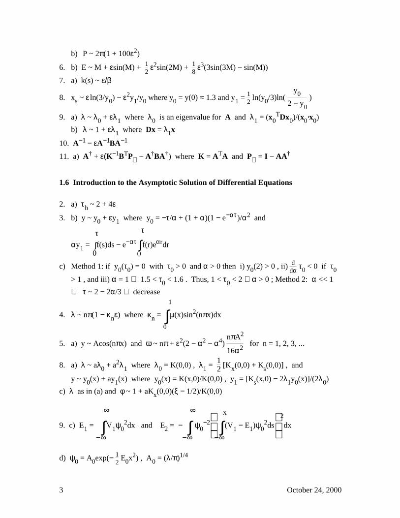
b) P ~ 2π(1 + 100ε2)
6. b) E ~ M + εsin(M) + 12 ε2sin(2M) + 1
8 ε3(3sin(3M) − sin(M))
7. a) k(s) ~ ε/β
8. xs ~ ε ln(3/y0) − ε2y1/y0 where y0 = y(0) ≈ 1.3 and y1 = 12 ln(y0/3)ln(
y0
2 − y0
)
9. a) λ ~ λ0 + ελ1 where λ0 is an eigenvalue for A and λ1 = (x0TDx0)/(x0·x0)
b) λ ~ 1 + ελ1 where Dx = λ1x
10. A−1 − εA−1BA−1
11. a) A† + ε(K−1BTP⊥ − A†BA†) where K = ATA and P⊥ = I − AA†
1.6 Introduction to the Asymptotic Solution of Differential Equations
2. a) τh ~ 2 + 4ε
3. b) y ~ y0 + εy1 where y0 = −τ/α + (1 + α)(1 − e−ατ)/α2 and
αy1 = ∫0
τf(s)ds − e−ατ ∫
0
τ
f(r)eαrdr
c) Method 1: if y0(τ0) = 0 with τ0 > 0 and α > 0 then i) y0(2) > 0 , ii) ddα τ0 < 0 if τ0
> 1 , and iii) α = 1 ⇒ 1.5 < τ0 < 1.6 . Thus, 1 < τ0 < 2 ∀ α > 0 ; Method 2: α << 1
⇒ τ ~ 2 − 2α/3 ⇒ decrease
4. λ ~ nπ(1 − κnε) where κn = ∫0
1
µ(x)sin2(nπx)dx
5. a) y ~ Acos(nπx) and ω ~ nπ + ε2(2 − α2 − α4) nπA2
16α2 for n = 1, 2, 3, ...
8. a) λ ~ aλ0 + a2λ1 where λ0 = K(0,0) , λ1 = 12 [Kx(0,0) + Ks(0,0)] , and
y ~ y0(x) + ay1(x) where y0(x) = K(x,0)/K(0,0) , y1 = [Ks(x,0) − 2λ1y0(x)]/(2λ0)
c) λ as in (a) and φ ~ 1 + aKx(0,0)(ξ − 1/2)/K(0,0)
9. c) E1 = ∫−∞
∞
V1ψ02dx and E2 = − ∫
−∞
∞
ψ0−2
∫−∞
x
(V1 − E1)ψ02ds
2
dx
d) ψ0 = A0exp(− 12 E0x2) , A0 = (λ/π)1/4
3 October 24, 2000
12. ∂tc0 + f(c0) = αg(t) where c0(0) = 0 and α = ∂Ω1/Ω
13. a) ii) L∂n* = ∂z + ε(f∂z2 − fx∂x − fy∂y ) + O(ε2) evaluated at z = 0
14. b) ρ ~ ε2n[(β − 1)(1 − s2)/2]n where r = 1 + εs
4 October 24, 2000

Chapter 2Matched Asymptotic Expansions
2.2 Introductory Example
1. a) y ~ ax + (1 − a)(1 − e−x/ε)
2. a) BL at x=0; y ~ (3 + x)−1/2 − e−2x−/ 3 where x− = x/ε
b) BL at x=0; y ~ g(x) − g(0)e−x− where g(x) = 1 − ∫x
1
f(s)ds and x− = x/ε
c) BL at x=0; y ~ ε(1 + 2x + 2e−x−)/3 where x− = x/ε
d) BL at x = 0; y ~ sech(1)[ − sinh(1) − e−x + (1 + e)e−x−] where x− = x/ε
e) y ~ −3x + 4(5 − 3e−4x−)/(5 + 3e−4x−) where x− = x/ε1/2
g) y ~ (1 + 7x2)1/3 − 21/23/[sinh(z) + 21/2] where z = 31/2x/ε + arcsinh(23/2)
8. a) y ~ βF(x,1) − ∫x
1F(x,r)g(r)dr + e−p(0)x/ε[α − βF(0,1) + ∫
0
1F(0,r)g(r)dr ] where g(r) =
f(r)/p(r) and F(x,r) = exp( ∫x
rq(s)/p(s)ds)
9. a) y ~ 1 + ae x − κ−1(1 + a) ∫x−
∞
e−s3/2ds where x− = x/ε2/3 , a = 2e−1 , and
κ = 23 Γ( 2
3 )
11. a) y ~ f(x) − f(0)exp(−x_2/2) where x
_ = x/ε1/2
b) y ~ f(x) − f(0)exp(−q(0)x_2/2) where x
_ = x/ε1/2
12. a) y ~ γ(γ − 1)−1[f(t) − f(0)e−t−] + g(λ)e−t− + γ[g0 − (γ − 1)−1f(0)][eγ−1(1−γ)t− − e−t−]
where t− = t/ε
13. ∂tc0 + f(c0) = αg(t) where c0(0) = Ω−1 ∫Ω
h(x)dV and α = ∂Ω1/Ω
15. a) y ~ x + 12z/(1 + z)2 where z = e21/2x/ε
5 October 24, 2000
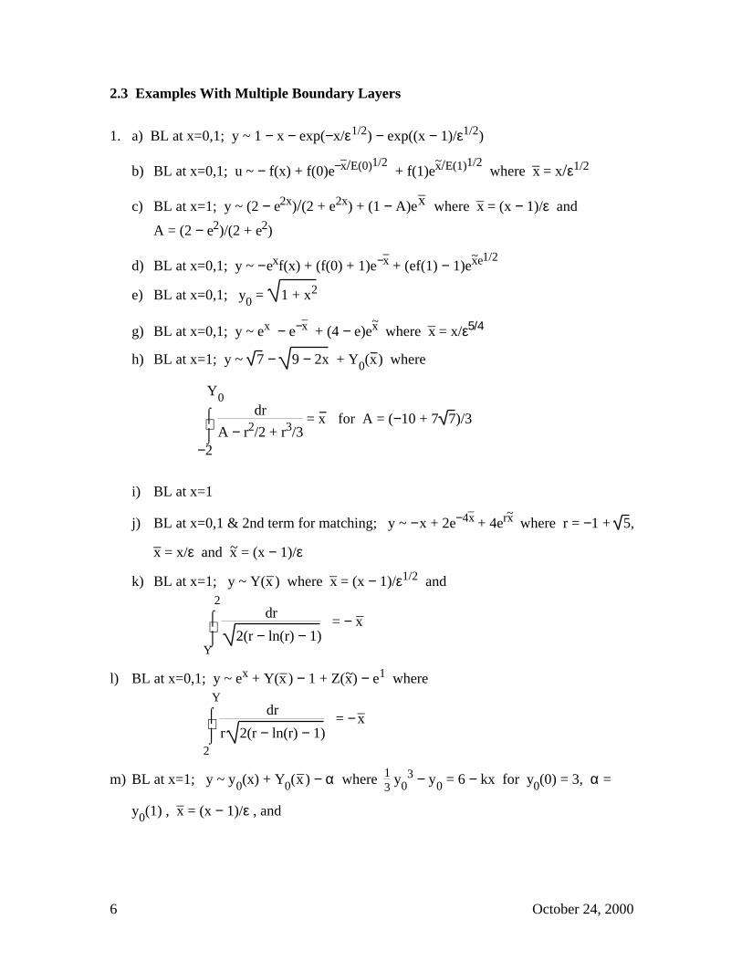
2.3 Examples With Multiple Boundary Layers
1. a) BL at x=0,1; y ~ 1 − x − exp(−x/ε1/2) − exp((x − 1)/ε1/2)
b) BL at x=0,1; u ~ − f(x) + f(0)e−x_/E(0)1/2
+ f(1)ex~/E(1)1/2 where x
_ = x/ε1/2
c) BL at x=1; y ~ (2 − e2x)/(2 + e2x) + (1 − A)ex_
where x_ = (x − 1)/ε and
A = (2 − e2)/(2 + e2)
d) BL at x=0,1; y ~ −exf(x) + (f(0) + 1)e−x_
+ (ef(1) − 1)ex~e1/2
e) BL at x=0,1; y0 = 1 + x2
g) BL at x=0,1; y ~ ex − e−x_
+ (4 − e)ex~ where x_ = x/ε5/4
h) BL at x=1; y ~ 7 − 9 − 2x + Y0(x−) where
⌡⌠
−2
Y0
dr
A − r2/2 + r3/3 = x− for A = (−10 + 7 7)/3
i) BL at x=1
j) BL at x=0,1 & 2nd term for matching; y ~ −x + 2e−4x_
+ 4erx~ where r = −1 + 5,
x_ = x/ε and x~ = (x − 1)/ε
k) BL at x=1; y ~ Y(x_
) where x_ = (x − 1)/ε1/2 and
⌡⌠
Y
2
dr
2(r − ln(r) − 1) = − x
_
l) BL at x=0,1; y ~ ex + Y(x_
) − 1 + Z(x~) − e1 where
⌡⌠
2
Y
dr
r 2(r − ln(r) − 1) = − x
_
m) BL at x=1; y ~ y0(x) + Y0(x_
) − α where 13 y0
3 − y0 = 6 − kx for y0(0) = 3, α =
y0(1) , x_ = (x − 1)/ε , and
6 October 24, 2000

⌡⌠
2
Y0
4dr
(r2 − α2)(r2 + α2 + 2) = x
_
2. BL at x = 0,1; y ~ κ0−1(1 − e−(x+1)/ε − e(x−1)/ε) and κ ~ κ0 + ... ⇒ κ0 = 21/3
3. a) y ~ H(0)/H(x) + Y0(x_
) − H(0)/H(1) where x_ = (x − 1)/ε and
x_/H(1) = H(1)(Y0 − 1) + H(0)ln
H(0) − H(1)Y0
H(0) − H(1)
4. b) λ ~ n2π2(1 + 4ε + (12 + n2π2)ε2)
5. y ~ − f(x)/q(x) + (α + f0/q0)er0x/ε + (β + f1/q1)er1(x−1)/ε where f0 = f(0) , etc. and r0
= − p0 − p02 + q0 and r1 = − p1 + p1
2 + q1
6. a) γ = (β − α)/2
b) φ = εα + ε1/2γΦ(x,ε)
c) outer: φ ~ εα1/(2k+1) ; bdy layer at x = 0: Φ ~ − εκ/(B + kx−/(k+1)1/2)1/k where
κ = (2k + 1)/(2k + 2) , B = (−γ (k + 1)1/2)−k/(k+1) and x− = x/εκ ; solution symmetric
about x = 1/2
d) it's necessary to find the second term in the boundary layer to be able to match ]
e) γ = (β − αΩ)/∂Ω
2.4 Interior Layers
1. a) IL at x=1/2; y ~ erf( (x − 1/2)/ 2ε )
b) IL at x=0; y ~ −2/x for x ≠ 0 and Y ~ 4ε−1/2x_M(1,3/2,−x
_2) where x_=x/ε1/2
c) for 0 ≤ x ≤ 712
, y ~ ( 53 − x)−1 − 2B·DeBx
_
/(1 + DeBx_
) and for 712
≤ x ≤ 1 , y ~ −
( 12 + x)−1 + 2B/(1 + DeBx
_
) where B = 1213
, x_ = (x − 7
12 )/ε
d) BL at x = 0 and IL at x = 3/4 ; for 0 ≤ x ≤ 3/4 , y ~ Y0 − 3exp(−3x−/16) and for
3/4 ≤ x ≤ 1 , y ~ Y0 + [ (x − 1/4)1/2 − 1/ 2 ]/(x − 3/4)3/2 where
Y0 = 1 + κ[ Γ(−1/4)M(3/4, 1/2, −x~2/4) + Γ(1/4)M(5/4, 3/2, − x~2/4) ]
Also, κ−1 = 32ε3/4(3π)1/2 , x~ = (x − 3/4)/ε1/2 and x− = x/ε
7 October 24, 2000

e) IL at x = 12 ; for 1/2 ≤ x ≤ 1 , y ~ y0(x) + Y0(x
_) − α where y0 − 1
3 y0
3 = x/2 +
1/6 for −1 ≤ y0 ≤ −α, α = y0(1/2+) , x_ = (x − 1/2)/ε , and
⌡⌠
0
Y0
4dr
(r2 − α2)(r2 + α2 + 2) = x
_
f) IL at x0 = 1/2
2. y ~ 1 + (1 − x2)1/2 for 0 ≤ x < xs = 3/2 and y ~ 0 for xs < x < 1; near x = 1 , y ~
Y0 where (2 − 3/Y0)exp(3/(2Y0)) = 72 exp(3(x
_ − 1)/4) ; for x near xs , y ~ Z0
where 2/Z0 + 43 ln[ (3/2 − Z0)/Z0 ] = x~ + B for x~ = (x − xs)/ε
3. b) BL at x =0,1; y ~ k(2x − 1) + (−3 − k)ex~ − ke−x_
where x_ = x/ε and x~ = (x −
1)/ε
4. a) outer: y ~ 12 (k + (k2 + 4α)1/2) for k = 1 − α − x/2 ; bdy layer: x− = (x − 1)/ε , 4a
= 1 − 2α + (1 + 12α + 4α2)1/2 , 4b = − 1 + 2α + (1 + 12α + 4α2)1/2 , and 0 ≤ Y ≤ a
satisfies
( a − Y
a )a( b + Y
b )b = e2(a+b)x-
7. c) y = −2 + x/4 + λ ∫0
x
e−2rg(r)/εdr where g(r) = (r − a)(r − b) − r2/3 + ab and λ is an
ε dependent constant that makes y(1) = 3 . The desired conclusion comes from the
fact that λ → 0 if g(r) < 0 anywhere in the interval 0 ≤ r ≤ 1 . If λ → 0 then the
layer is at x = b.8. a) T = T∞b) T ~ 1 − εln(1 − t)
c) T ~ T∞ − εT1 where µ = ε−nexp(− (T∞ − 1)/(εT∞)) and
τ + τ0 = − ∫1
T1
r−nexp(r/T∞)dr
8 October 24, 2000

2.5 Corner Layers
1. a) CL at x=1/2; youter ~ 12 + |x − 1
2 | and yinner ~ 1
2 + ε[2ln(1 + ex
_) − x
_] for x
_ =
(x − 12 )/ε
b) CL at x=1/3; youter ~ −1 + 3|x − 13 |
c) CL at x=0; yR ~ −xe−x , yL ~ x(2e − e−x)
d) BL at x=0 and CL at x=5/8; yR = 0 for 0 < x ≤ 5/8 and yL = 1 − 9/4 − 2x for
5/8 ≤ x ≤ 1e) BL at x=0 and CL at x=1/2; yR = 1/2 for 0 < x ≤ 1/2 and yL = x for 1/2 ≤ x ≤ 1 ;
BL at x=0
2. YCL ~ 1 + εγα0( M(−γ, 1/2, −(b − a)x_2/2) − κx
_M(1/2 − γ, 3/2, −(b − a)x
_2/2) ) where
γ = a2(b − a)
and κ = 2(b − a) Γ(η + 1/2)/Γ(η) for η = b2(b − a)
3. BL at x = 0,1 and a CL at x = xs where xs ~ ε1/2 ln(3/y0(0)); y ~ y0(x) + 3ex~ for
xs < x ≤ 1 and y ~ 3e−x_
for 0 ≤ x < xs where x~ = (x − 1)/ε1/2 , x_ = x/ε1/2 and
⌡⌠
y0
2
dr
arctanh(r − 1) = 1 − x .
4. a) boundary layers at x = 0, 1 and a corner layer at x = 1/3
b) there is an interior layer at x = 13 2 − 3/8 and at x = 11/8 − 1
3 2
c) interior layer at x = 13 2 − 3/8 , a corner layer at x = 1/3 , and a boundary layer at x
= 1
2.6 Partial Differential Equations
4. a) u ~ h(x + s) + [g(t) − h(s)]exp[−xv(t)/ε] where s = ∫0
t
v(τ)dτ
b) the 2nd term in the outer expansion is u1(x, t) = th ′′(x + s)
7. b) X ~ s(t) + 2εln(B)/(u0+ − u0
− )
8. a) outer layers ( x ≠ 0 ): u ~ φ(x − αt)exp(− β2α (x + αt)) and shock layer:
9 October 24, 2000

u ~ 12 e−βt[ φ(0+)erfc(− z) + φ(0−)erfc(z) ] where z =
x − αt
2(εt)1/2
9. u0 = φ(x − f(u0)t) and ∂x_U0 = F(U0) − s′(t)U0 + A(t) where F ′ = f , s′ = (F(u0
+) −
F(u0−))/(u0
+ − u0−) and A = (u0
−F(u0+) − u0
+F(u0−))/(u0
+ − u0−)
12. c ~ 1r + µ erfc(
x
2t1/2 ) + (1 − 1
r + µ )erfc( x2ε
( r + µ
µt )1/2 )
2.7 Difference Equations
4. a) yn ~ Ar+n + Br−
n where r± = [−β ± (β2 + α2)1/2]/α
b) α = hpn/2 , β = h2qn/2 ; the 2nd derivative doesn't contribute
10 October 24, 2000
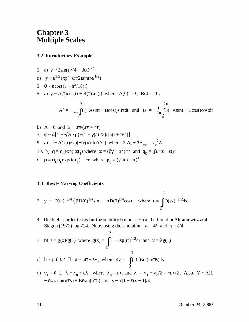
Chapter 3Multiple Scales
3.2 Introductory Example
1. a) y ~ 2sin(t)/(4 + 3εt)1/2
d) y ~ ε1/2exp(−αt/2)sin(t/ε1/2)
3. θ ~ εcos((1 − ε2/16)t)5. a) y ~ A(τ)cos(t) + B(τ)sin(t) where A(0) = 0 , B(0) = 1 ,
A ′ = − 12π ∫
0
2πF(−Asint + Bcost)sintdt and B′ = − 1
2π ∫0
2πF(−Asint + Bcost)costdt
b) A = 0 and B = 3π/(3π + 4τ)
7. φ ~ α[1 − 2exp(−(1 + γ)ε t /2)sin(t + π/4)]
9. a) φ ~ A(x,t)exp[−iv(x)sin(t/ε)] where 2iAt + 2Axx = vx2A
10. b) q = q0exp(iωt1) where ω = (βγ − α2)1/2 and q0 = (β, iω − α)T
c) p = α0p0exp(iωt1) + cc where p0 = (γ, iω + α)T
3.3 Slowly Varying Coefficients
2. y ~ D(εt)−1/4 (βD(0)3/4sinτ + αD(0)1/4cosτ) where τ = ∫0
t
D(εs)−1/2ds
4. The higher order terms for the stability boundaries can be found in Abramowitz andStegun (1972), pg 724. Note, using their notation, a = 4λ and q = ε/4 .
7. b) s = g(x)/g(1) where g(x) = ∫0
x
[1 + εµ(r)]1/2dr and ν = λg(1)
c) h ~ µ′(s)/2 ⇒ ν ~ nπ − εv1 where 4v1 = ∫0
1
µ′(s)sin(2nπs)ds
d) ν1 = 0 ⇒ λ ~ λ0 + ελ1 where λ0 = nπ and λ1 = v1 − v0/2 = −nπ/2 . Also, Y ~ A(1
− εs/4)sin(nπs) + Bεsin(nπs) and s ~ x[1 + ε(x − 1)/4]
11 October 24, 2000

3.4 Forced Motion Near Resonance
1. a) u ~ α + (α0 − α)sin(θ − εαθ + π/2)
b) 2π(1 + α2ε)
c) ∆φ ≈ 42.98"
2. b) A∞2[9λ2 + (6ω − 3κ
4 A∞
2)2] = 1 ⇒ AM = (3λ)−1
3. a) y ~ A(εt)cos(t + θ0) where A = 2 or A = 2[c/(c + 4exp(−ε t))]1/2
4. a) θ ~ ε2(sinωt − ωsint)/(1 − ω2) + O(ε8)
b) 2A ′ = − cos(θ − ωεt) and A∞3 + 16ωA∞ ± 8 = 0
5. y ~ ε1/3A(εt)cos[κt + θ(εt)] where A∞( 3λ8
A∞2 − 2ωκ) = 1
6. a) y ~ ε1/3A(ε2/3t)cos[t + θ(ε2/3t)] where A∞2[α2 + (2ω + A∞
2)2] = 1
b) yes
7. a) y ~ f(v)(1 − e−γεtcos(t)) where γ = β + a(v2 − 1)
b) y ~ ε−1A(εt)cos(t + θ0) where 2A ′ + [β + a(v2 − 1 + 14 A2)]A = 0
Other references: Derjaguin, et al. (1957) and Vatta (1979)
10. a) θ ~ ε1/2A(εt)cos[t + φ(εt)] where 8A′ = [αsin(2φ) − 4µ]A and if A ≠ 0 then
16φ′ = 2αcos(2φ) − A2 − 4α . Note, α < 4µ ⇒ A → 0
3.6 Introduction to Partial Differential Equations
5. a) u(x,t) ~ ∑n=1
∞ βne−εt/2cos((λn
2 − ε/2)t)sinλnx
8. b) u ~ ε(1 − x)U(τ) and ρ ~ (1 − ∫0
τ
U(σ)dσ)−1
3.7 Linear Wave Propagation
1. u ~ [c(0)/c(εt)]1/2[ f(x − ∫0
t
c(ετ)dτ) + f(x + ∫0
t
c(ετ)dτ) ]/2
12 October 24, 2000
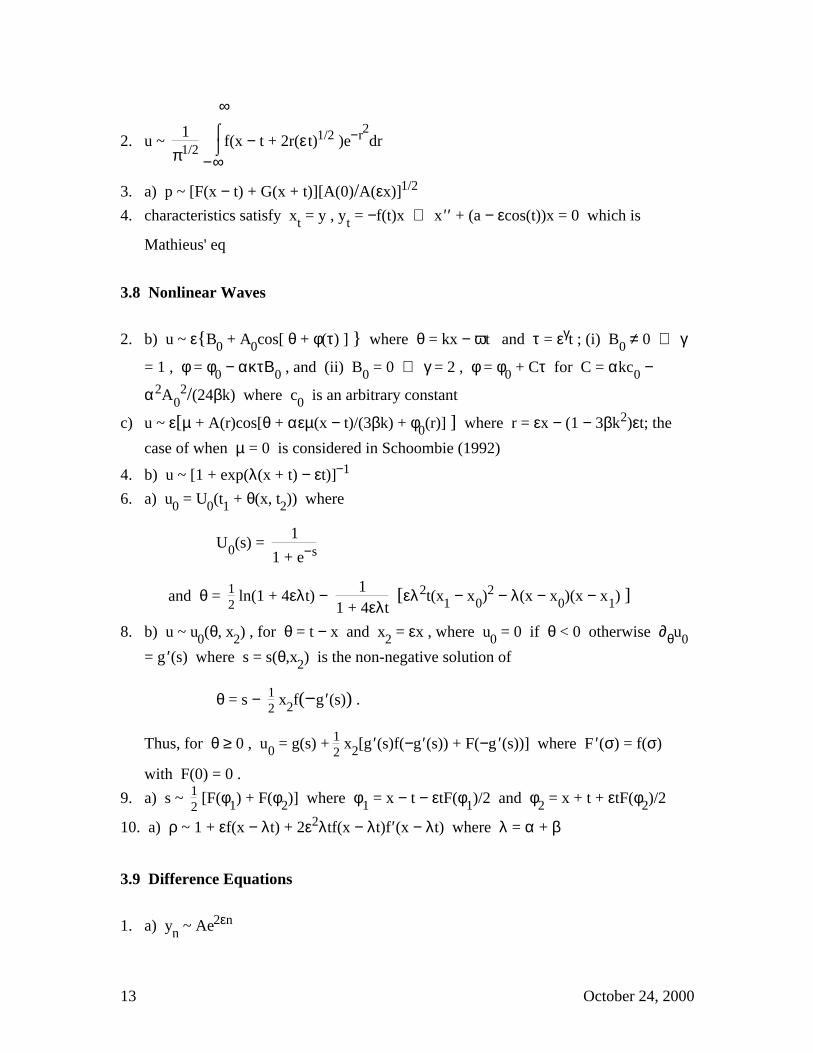
2. u ~ 1
π1/2 ⌡
⌠
−∞
∞
f(x − t + 2r(ε t)1/2 )e−r2dr
3. a) p ~ [F(x − t) + G(x + t)][A(0)/A(εx)]1/2
4. characteristics satisfy xt = y , yt = −f(t)x ⇒ x ′′ + (a − εcos(t))x = 0 which is
Mathieus' eq
3.8 Nonlinear Waves
2. b) u ~ εB0 + A0cos[ θ + φ(τ) ] where θ = kx − ωt and τ = εγt ; (i) B0 ≠ 0 ⇒ γ
= 1 , φ = φ0 − ακτΒ0 , and (ii) B0 = 0 ⇒ γ = 2 , φ = φ0 + Cτ for C = αkc0 −
α2A02/(24βk) where c0 is an arbitrary constant
c) u ~ ε[µ + A(r)cos[θ + αεµ(x − t)/(3βk) + φ0(r)] ] where r = εx − (1 − 3βk2)εt; the
case of when µ = 0 is considered in Schoombie (1992)
4. b) u ~ [1 + exp(λ(x + t) − εt)]−1
6. a) u0 = U0(t1 + θ(x, t2)) where
U0(s) = 1
1 + e−s
and θ = 12 ln(1 + 4ελt) −
11 + 4ελt
[ελ2t(x1 − x0)2 − λ(x − x0)(x − x1) ]
8. b) u ~ u0(θ, x2) , for θ = t − x and x2 = εx , where u0 = 0 if θ < 0 otherwise ∂θu0
= g ′(s) where s = s(θ,x2) is the non-negative solution of
θ = s − 12 x2f(−g ′(s)) .
Thus, for θ ≥ 0 , u0 = g(s) + 12 x2[g ′(s)f(−g′(s)) + F(−g ′(s))] where F ′(σ) = f(σ)
with F(0) = 0 .
9. a) s ~ 12 [F(φ1) + F(φ2)] where φ1 = x − t − εtF(φ1)/2 and φ2 = x + t + εtF(φ2)/2
10. a) ρ ~ 1 + εf(x − λt) + 2ε2λtf(x − λt)f′(x − λt) where λ = α + β
3.9 Difference Equations
1. a) yn ~ Ae2εn
13 October 24, 2000
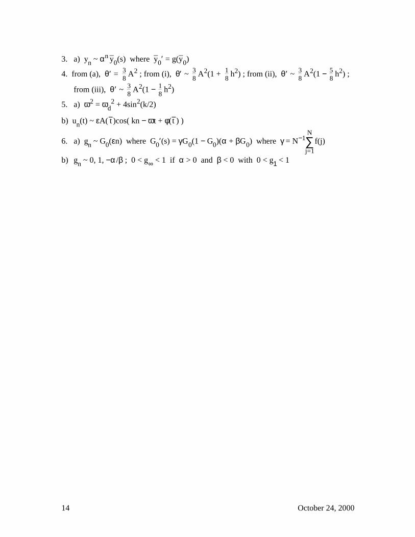
3. a) yn ~ αn y_
0(s) where y_
0′ = g(y_
0)
4. from (a), θ′ = 38 A2 ; from (i), θ′ ~ 3
8 A2(1 + 1
8 h2) ; from (ii), θ′ ~ 3
8 A2(1 − 5
8 h2) ;
from (iii), θ′ ~ 38 A2(1 − 1
8 h2)
5. a) ω2 = ωd2 + 4sin2(k/2)
b) un(t) ~ εA( t−)cos( kn − ωt + φ(t−) )
6. a) gn ~ G0(εn) where G0′(s) = γG0(1 − G0)(α + βG0) where γ = N−1∑j=1
Nf(j)
b) gn ~ 0, 1, −α/β ; 0 < g∞ < 1 if α > 0 and β < 0 with 0 < g1 < 1
14 October 24, 2000
Chapter 4The WKB and Related Methods
4.2 Introductory Example
1. c) ywkb ~ A[exp(−ex) − exp(ex − 2 − x/ε)] where
A = (exp(−e) − exp(e − 2 − 1/ε))−1 and ycom ~ exp(e − ex) − exp(−1 + e − x/ε)
3. d) y ~ q−1/4(Aeη/ε + Be−η/ε)exp(− 12 ∫xf(r)dr) where η = ∫
x
q(r)dr
4. c) y ~ h−1/2[ a0exp( 12ε
⌡⌠x
(− p + h + εp′h )ds + b0exp(−
12ε
⌡⌠x
(p + h + εp′h )ds ]
where h = (p2 − 4q)1/2
7. c) w ~ g(x)[ (a + b/n)sin(λnθ) − acos(λnθ)
2λn∫
0
x
(pq)−1/2(f − 2qλ0λ2 − pg ′′/g)ds ] where
a,b are arbitrary constants, θ = ∫0
x
(q/p)1/2ds and λ0 = π/κ
e) λ ~ n(1 − 49
72(nπ)2 )
8. y± ~ q−1/4exp[ 12ε
∫x
(±(−4q + εp2)1/2 − ε1/2p)dx ]
10. a) y± ~ κ±x±ν[1 −+ 14ν (α± + x2) + ...
b) Jν(x) ~ (2πν)−1/2 ( ex2ν
)ν [1 − 1
12ν (1 + 3x2) ]
11. a) y ~ εet/2 sin[α(1 − e−t)] + 18 ε(et − 1)cos[α(1 − e−t)] where α = 1/ε
b) two principal shortcomings are: (1) differences in zeros --- this is a relatively minor
problem as discussed in Section 1.4, and (2) unboundedness of second term for large
t --- in particular, we need εet << 1 . The latter problem is due to a turning point at t
= ∞ .
c) y = π2 [Y0(α)J0(β) − J0(α)Y0(β)] where α = 1/ε and β = αe−t
12. a) εβR′′ + (−1 + λβ)R′ = 0 and εβR ′(0) − R(0) = 0 ⇒ R = 1 − re−kx/ε where r =
1/(βλ) and k = (−1 + λβ)/β
15 October 24, 2000
b) R ~ 1 + Ae−θ(x)/ε(1 − λβ)−1 where θ = λx − ∫0
x
β−1(s)ds and
A = 1 − (λβ0)−1 ; the conditions are that θ → ∞ as x → ∞ and λβ > 0 for 0 < x < ∞
13. P ~ A(x,ε)exp( θ(x)/ε + ηµ0x(eθx − 1) − ∫
0
ηλ(s)ds ) where θx = ln(ξ) and ξ(x)
satisfies 1 = µ0x ∫0
∞
exp( µ0x(ξ − 1)η − ∫0
h
λ(s)ds )dη . Also, A is determined from
the O(ε) term from the η = 0 condition
4.3 Turning Points
3. b) E = ε(2n + 1)µ1/2
d) E ~ (αµεmN2)1/γ (1 + β/N2) where 4α = π( Γ( 3m+22m
)/Γ( m+1m
))2 and 3π(m +
2)2β = 4m(m − 1)cot(π/m)
4. b) the approximation for ψ(x) is given by (4.44) for x < a , and for x > b one finds
Ψ ~ 2aRq(x)− 1/4e−φ/εexp(i(− Et − θ−/ε − π/4)) where q = V(x) − E ,
φ = ∫a
b
q(s) ds and θ− = ∫x
b
q(s) ds
8. b) balancing ⇒ α = 1/2 and β = 1/4
4.4 Wave Propagation and Energy Methods
4. b) E = 12 Du2
xx + 12 µu2
t , S = −uxtDuxx + ut∂x(Dux) , Φ = 0
4.5 Wave Propagation and Slender Body Approximations
1. a) for the nth mode the general solution has the same form as in (4.84) but
uL = sin(λny)
θx
aLei[ωt − θ(x)/ε] + ζ(x) + bLei[ωt + θ(x)/ε] − ζ(x)
16 October 24, 2000

where θ(x) is given in (4.87) and ζ(x) = ω2 ∫
0
x
α(x)(ω2µ2 − λn)−1/2 dx
4.6 Ray Methods
1. a) It's not hard to show that aidi + ardr + atdt = 0 where ai, ar, at are not all zero.
b) Using the t, n, txn coordinate system, where t is the unit tangent to S in the plane ofincidence which satisfies t·di > 0 , then θI = µ+di·x , θR = µ+dr·x , and θT = µ−dt·x ⇒
uI = (α, −β, 0) , uR = (α, β, 0) and uT = (κα, −(1 − κ2α2)1/2, 0) where κ = µ+/µ− and
β = (1 − α2)1/2
3. a) D(∇θ·∇θ)2 = µ
4. b) SIAM Appl Math, v16, 1968, 783-8075. a) α = µ(−1/2)sin(ϕ) where zR = min0, roots of µ(z) = α for z > −1/2
c) v0 = [tanϕ/(µJ)]1/2/(4π)
7. a) µ = constant ⇒ rays are straight lines ⇒ wave fronts parallel ⇒ Ri = ρi + s ;
in R2 , ρ2 = ∞
8. a) (4.103) ⇒ x_
ss = ax_ − bx
_s ⇒ ps = 0
b) κ = ±r0µ(r0)sin(φ0) where φ0 is the initial angle the ray makes with the radius
vector10. c) note κ ≈ 0.065rc where rc is the scale factor (in km) used to nondimensionalize
r* = rcr
4.8 Discrete WKB Method
6. a) yn ~ (qn2 − 4)−1/4[a0exp(θ+/ε) + b0exp(θ−/ε)] where
θ± = ⌡⌠εn
ln[ 12 (q(ν) ± q(ν)2 − 4 ) ]dν .
b) αn+1 = (cn/an)αn−1
7. a) yn ~ (1 − ν2)−1/4(a0exp(iθ/ε) + b0exp(− iθ/ε)) where ν = εn and
17 October 24, 2000

θ = νcos−1(ν) − (1 − ν2)1/2
b) a0 = (ε/2π)1/2exp(iπ/4) and b0 = (ε/2π)1/2exp(− iπ/4)
8. a) zn ~ ν1−α/2(1 + 4ν)−1/2(arn + b/rn) where ν = εn and
rn = ( 1 + 2ν + (1 + 4ν)1/2
ν )n−α/2
exp( (1 + 4ν)1/2
2ε )
9. b) γ = k − n and R ~ eθ(κ)/ε[ R0(n,κ) + ... ] , where θ = κ + (1 − κ)ln(1 − κ) and
R0 = A[(1 − κ)en]en/2 .
18 October 24, 2000

Chapter 5The Method of Homogenization
5.2 Introductory Example
2. a) ∂x(D_
∂xu0) + g(u0) = ∂tu0 + ⟨f⟩∞8. e) ⟨⟨D−1⟩⟩∞
−1 = 1/(φα/Dα + φβ/Dβ) which is a volume fraction weighted harmonic
mean ; the harmonic mean is obtained only when φα = φβ = 1/2
f) the greatest relative error occurs when φα = 1/2 with a relative absolute error of
(Dα − Dβ)2/(4DαDβ) ; the error is zero if φα = 0 or if φα = 1
5.4 Porous Flow
3. b) setting wq = (uq, vq, wq) for q = s,f ⇒ ∇2wq = 0 where wq is periodic and on
the interface Dsn·(e1 − ∇yus) = αDfn·(e1 − ∇yuf) etc
4. b) ( ∇2y − z
2αezφ0)f = zαe
zφ0 where n·∇yf = 0 on ∂Ωf
e) φ satisfies the Poisson-Boltzmann equation ∇2yφ = zαezφ in Ωf where φ is
periodic and n· yφ = σ on ∂Ωf .
19 October 24, 2000
Chapter 6Introduction to Bifurcation and Stability
6.2 Introductory Example
1. b) y± = ±(1 − 4λ2)1/2/3 for −1 ≤ 2λ ≤ 1 where y+ stable and y− unstable
3. a) supercritical pitchfork when λn = (nπ)2 and θn ~ 2(2ε)1/2cos(nπx)/(nπ)
b) V1 ~ −2ε2/π2 ⇒ θs = 0 unstable for λ > π2
c) for θn one finds Vn ~ −2ε2/(nπ)2 ⇒ V1 < V2 < ... < Vn < 0 and this suggests V1
is the preferred configuration
4. a) y = Asin(nπx) where A = 0 or A2 = 2(λ − (nπ)2) ; pitchfork bifurcation at (λp,
Ap) = ((nπ)2, 0) for n = 1, 2, 3, ...
b) Vn = − An4/2
5. a) θ = 0 stable for 0 < ω < 1 and θ = ±arccos(ω−2) stable for 1 < ω < ∞ ; θ = ±π
unstable6. c) κ0 = 0 and 0 < κ1 < 1/2
d) slope for Ω = 40 is 24.34 and slope for Ω = 30 is 20.36 ; ω = ε(1/2 − κ2)1/2Ω
7. c) ω = 2 and v ~ A(τ)cos(t + θ(τ)) where A = A0(α02 + e−3τ)1/2e3τ/4 and θ = −π/4
+ arctan(α0e3τ/2)
6.5 Relaxation Dynamics
3. b) ln(y0) − 12 y0
2 = t + 12 (ln3 − 3) and the corner is at t = 1 − 1
2 ln3 , y = 1 and v =
−2/3
d) T ~ 3 − 2ln2 ≈ 1.614
5. a) subcritical saddle-node at (λb, gb) ≈ (0.1292, 0.0635)
6. a) supercritical saddle-node at (λ0 , y0) ≈ (280.76, 2.360) and subcritical saddle-
node at (λ1 , y1) ≈ (336.6, 6.6355)
c) Y~
~ y1 − σε1/3(a0Ai ′(−ξτ~) + a1Bi′(−ξτ~))/(a0Ai(−ξτ~) + a1Bi(−ξτ~)) where σ =
ξ/(15y1 − 74) , ξ = [(15y1 − 74)(y1 − 1)]1/3 and τ~ = (τ − λ1)/ε2/3 ⇒ τ0 = λ1 +
(2.3381...)ε2/3/ξ
20 October 24, 2000

7. a) transcritical bifurcation at (0,0) and a subcritical saddle-node at (9/8, 3/4)
c) y ~ ys + ε1/3Acos(ωt + θ) where A∞2 κ2ω2 + 9
4 A∞
4[ −1 + 7(1 − 2ys)2/ω2]2 = 1
6.6 An Example Involving A Nonlinear Partial Differential Equation
1. a) us = ±ε1/2Asin(nx) and λb = n2 where A = 2/ 3
b) us = 0 stable for λ < 1 and us = ±ε1/2Asin(x) stable for 0 ≤ λ − 1 << 1
2. a) us = εαAsin(nπx) and λb = (nπ)2 , where (i) n odd ⇒ A = 3/(8nπ) and α = 1 ,
and (ii) n even ⇒ A2 = 6/(5λb) and α = 1/2
b) stable for λ < π2
Additional References: Bramson (1983) and Fisher (1937)
3. a) (i) us = 0 ∀ λ , and (ii) us = Ansin(nπx) with λ = λn(1 + An2/8) where λn =
(nπ)2
b) unbuckled state is stable if λ < π2 and unstable if λ > π2
6. b) κ = 0 and stable for λ < 1
c) v ~ ε[B0 + A0cos((1 + 12 ε)x + θ0)] and κ ~ 1
4 A0
2ε2 where ε = λ − 1
8. c) u0 = (ui + uj)/2 , αij = −(ui − uj)/2 , βij = (1/8)1/2(uj − ui) , and χij = 21/2sgn(uj −ui)(u1 + u2 + u3 − 3u0) ; see Albano, et al. (1984)
9. b) for 0 ≤ λ < 7 the steady states are ui = αix , for α1 < α2 < α3 , where u1,u3 are
stable and u2 is unstable; for 7 < λ the steady state u3 is unique and stable
10. a) u ~ us + ∑vneint ⇒ λ < 1
6.7 Bifurcation of Periodic Solutions
1. a) saddle-node at (−1/4,−1/2) , a Hopf at (0,0) , and a transcritical at (0,−1)
b) y ~ ε1/2Acos(t1 + θ) where 8A′ = A(4 − A2) and 24θ′ = 36 − 31A2 ]
2. a) ys = 0 asy. stable only when λ < 0
b) y ~ A(εt)sin(t + θ0) where A(τ) = 1/( α0α + cexp(−nτ) )1/2n
3. b) y = 0 unstable; y = y0 stable for 0 < rT < π/2 and for rT > π/2 there are stable
limit cycles4. b) y = y0 is stable for λy0 < 2 and there's a Hopf bifurcation at λy0 = 2
21 October 24, 2000
6.8 Systems of Ordinary Differential Equations
3. a) r′ = − r(r2 − λ(1 − λ)) and θ′ = − 1
4. a) y = v = (1 − α − β + µ)/2
5. a) y = v = 1 is stable for λ < (γ − 1)-1 and unstable for λ > (γ − 1)−1
b) a Hopf bifurcation takes place
6. a) x = γ/(1 − γ) , n2 = (1 − γ)/α is stable for (1 − γ)3 < 4α7. a) cs = Tsexp(−Ts) and Ts = µ/κ ; steady state is asymptotically stable if κ > (Ts −
1)exp(−Ts)
b) supercritical Hopf bifurcation at µl and subcritical Hopf bifurcation at µr
d) µl ~ κ(1 + eκ + e2κ2 + ...) and µr ~ κ(ζ − ζ−1 − 1.5ζ−2 + ... ) where ζ > 1 satisfies
ζexp(−ζ) = κ ⇒ ζ ~ z0 + ln(z0) + ln(z0)/z0 where z0 = ln(κ−1)
8. a) xs = µ/α , ys = α/µ is stable
b) xs = µ/α , ys = α/µ is stable if µ > µc and it's unstable if 0 < µ < µc ,
where µc = α(1 − α)1/2
9. a) θ = z = 0
b) θ = 0 and z = εα0cos(κt) ; the motion is straight up and down; see van der Burgh
(1968)10. a) λ < 0
b) k2 = λ − r02 and 0 < r0 < λ1/2
11. a) Hopf bifurcation along line λ = − µ for − 1 < µ < 1
b) y ~ ε1/2y0(t,τ) and v ~ ε1/2v0(t,τ) where τ = εt . As t → ∞ , y0 → sin(Θ) and v0
→ (1 − µ2)1/2cos(Θ) + µ sin(Θ) where Θ = (1 − εµ)(1 − µ2)1/2 t + θ0
22 October 24, 2000