Technische Universit at Graz

Stabilized Boundary Element Methodsfor Exterior Helmholtz Problems

S. Engleder, O. Steinbach

Berichte aus demInstitut fur Numerische Mathematik

Bericht 2007/4

Technische Universit at Graz

Stabilized Boundary Element Methodsfor Exterior Helmholtz Problems

S. Engleder, O. Steinbach

Berichte aus demInstitut fur Numerische Mathematik

Bericht 2007/4

Technische Universitat GrazInstitut fur Numerische MathematikSteyrergasse 30A 8010 Graz

WWW: http://www.numerik.math.tu-graz.ac.at

c© Alle Rechte vorbehalten. Nachdruck nur mit Genehmigung des Autors.

Stabilized Boundary Element Methods

for Exterior Helmholtz Problems

S. Engleder, O. Steinbach

Institut fur Numerische Mathematik, TU Graz,Steyrergasse 30, A 8010 Graz, Austria

sarah.engleder, o.steinbach@tugraz.at

Abstract

In this paper we describe and analyze some modified boundary element methodsto solve exterior boundary value problems for the Helmholtz equation with eitherDirichlet or Neumann boundary conditions. The proposed approach avoids spuriousmodes even in the case of Lipschitz boundaries. Moreover, the regularisation is donebased on boundary integral operators which are already available in standard bound-ary element formulations. Numerical examples are given to compare the proposedapproach with other already existing regularized formulations.

1 Introduction

The boundary integral formulation [2, 9, 13] of exterior boundary value problems for theHelmholtz equation with either Dirichlet or Neumann boundary conditions may lead toboundary integral equations which are either not uniquely solvable, or not solvable at all. Inparticular we will have spurious modes if the wave number corresponds to an eigenvalue ofthe interior eigenvalue problem for the Laplace operator with either homogeneous Dirichletor Neumann boundary conditions, respectively.

Hence one may use combined boundary integral formulations such as the indirectBrakhage–Werner approach [5], or the direct Burton–Miller formulation [8] to obtainboundary integral equations which are uniquely solvable for all wave numbers. The abovementioned combined boundary integral formulations are usually analyzed in L2(Γ) by usingsome compactness arguments for the Laplace double layer potential. Hence this approachis restricted to the case of sufficiently smooth boundaries.

When introducing appropriate regularization operators one can formulate modifiedboundary integral equations where the unique solvability can be ensured even for Lipschitzdomains when considering the resulting integral equations in the energy spaces H1/2(Γ)and H−1/2(Γ), respectively, see, e.g., [6, 7]. For other regularisation procedures, see forexample [3, 4, 21].

1

In [10] we have proposed an alternative modified boundary integral equation which isbased on the use of standard boundary integral operators only. The unique solvabilityof the proposed combined boundary integral equation follows from a Gardings inequalitywhile the injectivity is based on some mapping properties of the underlying boundaryintegral operators. Here we extend our previous approach to a coupled system which isequivalent to the above mentioned combined boundary integral equation. In particularwe prove a Garding’s inequality also for the system which enables us to use standardarguments [16, 19, 20, 22] to analyze a Galerkin discretization scheme for the system. Notethat the Galerkin discretization of the coupled system also defines an approximation of theGalerkin discreitization of the combined boundary integral equation.

This paper is organized as follows: In Section 2 we recall different combined and regu-larized boundary integral formulations for the exterior Dirichlet boundary value problemof the Helmholtz equation. In particular we prove the unique solvability of a coupledsystem of boundary integral equations. Galerkin boundary element method is formulatedand analyzed in Section 3, again for the Dirichlet problem. In Section 4 we summarizethe corresponding modified boundary element method for the exterior Neumann boundaryvalue problem. Numerical results for the proposed modified boundary element methodsand comparisons with other existing approaches are finally discussed in Section 5.

2 Boundary Integral Equations

As a model problem we consider the exterior Dirichlet boundary value problem for theHelmholtz equation,

∆u(x) + κ2u(x) = 0 for x ∈ Ωc = R3\Ω, u(x) = g(x) for x ∈ Γ = ∂Ω, (2.1)

where in addition

limR→∞

∫

∂BR

∣∣∣∣∂

∂nyu(y)− iκu(y)

∣∣∣∣2

dsy = 0 (2.2)

is the Sommerfeld radiation condition. Moreover, κ ∈ R+ is the wave number, Ω ⊂ R3 is

a bounded Lipschitz domain, and g ∈ H1/2(Γ) are some prescribed Dirichlet data.By using the fundamental solution of the Helmholtz equation in R

3,

U∗κ(x, y) =

1

4π

eiκ|x−y|

|x− y| for x 6= y,

we can find different representations to describe the unique solution of the boundary valueproblem (2.1). In particular when using an indirect approach we can represent the solutioneither by means of the single layer potential

u(x) = (Vκw)(x) =

∫

Γ

U∗κ(x, y)w(y)dsy for x ∈ Ωc (2.3)

2

where w ∈ H−1/2(Γ) is some unknown density function, or we can describe the solution of(2.1) by means of the double layer potential

u(x) = (Wκv)(x) =

∫

Γ

∂

∂nyU∗

κ(x, y)v(y)dsy for x ∈ Ωc (2.4)

where v ∈ H1/2(Γ) is again some unknown density function. When using a direct approach,the solution of (2.1) is given by the representation formula

u(x) = −∫

Γ

U∗κ(x, y)

∂

∂nyu(y)dsy +

∫

Γ

∂

∂nyU∗

κ(x, y)u(y)dsy for x ∈ Ωc. (2.5)

When applying the exterior trace operator γext0 to the single and the double layer potentials

Vκ and Wκ we obtain certain boundary integral equations for the yet unknown densityfunctions w ∈ H−1/2(Γ), v ∈ H1/2(Γ), and t = ∂

∂nu ∈ H−1/2(Γ), respectively. In particular,

when using the single layer potential (2.3) we have to solve the first kind boundary integralequation

(Vκw)(x) := γext0 (Vκw)(x) =

∫

Γ

U∗κ(x, y)w(y)dsy = g(x) for x ∈ Γ, (2.6)

for the double layer potential (2.4) we obtain the second kind boundary integral equation

(1

2I+Kκ)v(x) := γext

0 (Wκv)(x) =1

2v(x)+

∫

Γ

∂

∂nyU∗

κ(x, y)v(y)dsy = g(x) for x ∈ Γ, (2.7)

and for the direct formulation (2.5) we finally get the first kind boundary integral equation

(Vκt)(x) = (−1

2I +Kκ)g(x) for x ∈ Γ. (2.8)

It is well known that if κ2 = λ corresponds to an eigenvalue of the interior Dirichleteigenvalue problem

−∆uλ(x) = λuλ(x) for x ∈ Ω, uλ(x) = 0 for x ∈ Γ, (2.9)

the boundary integral equations (2.6) and (2.8) are not uniquely solvable, and if κ2 = µ

corresponds to an eigenvalue of the interior Neumann eigenvalue problem

−∆uµ(x) = µuµ(x) for x ∈ Ω,∂

∂nx

uµ(x) = 0 for x ∈ Γ, (2.10)

the boundary integral equation (2.7) is not uniquely solvable.

3

2.1 Modified Boundary Integral Equations

The idea of using combined boundary integral equations to overcome the problem of non–unique solvability goes back to Brakhage and Werner in 1965 [5]. They used the followingrepresentation formula

u(x) = (Wkw)(x) − iη(Vkw)(x) for x ∈ Ωc (2.11)

with an unknown density function w ∈ L2(Γ) and η > 0, which leads to the boundaryintegral equation

(1

2I +Kκ)w(x) − iη(Vκw)(x) = g(x) for x ∈ Γ. (2.12)

For domains Ω with a smooth boundary Γ = ∂Ω it can be shown [5] that the boundaryintegral operator corresponding to (2.12)

1

2I +Kκ − iηVκ : L2(Γ) → L2(Γ) (2.13)

is coercive and injective, i.e. (2.12) admits a unique solution w ∈ L2(Γ).In addition to the weakly singular boundary integral equation (2.8) we also consider

the hypersingular boundary integral equation

(1

2I +K ′

κ)t(x) = −(Dκg)(x) for x ∈ Γ. (2.14)

Combining the direct boundary integral equations (2.8) and (2.14), this gives the Burton-Miller formulation [8]

[Vκ − iη

(1

2I +K ′

κ

)]t(x) =

[iηDκ +

(−1

2I +Kκ

)]g(x) for x ∈ Γ. (2.15)

Note that the unique solvability of (2.15) in L2(Γ) follows as for the Brakhage–Wernerformulation (2.12). But the problem is that the coercivity of the operator (2.13) in L2(Γ)does not carry over to domains with a non–smooth boundary. Therefore there is a need toconsider the density function w as an element ofH−1/2(Γ), and to introduce a regularisationoperator B : H−1/2(Γ) → H1/2(Γ), which lifts w in the right energy space, see, e.g. [6, 7].Hence we obtain the representation formula

u(x) = (Vκw)(x) + iη(WκBw)(x) for x ∈ Ωc

and thus the boundary integral equation to be solved

(Vκw)(x) + iη(1

2I +Kκ)Bw(x) = g(x) for x ∈ Γ.

4

In [6, 7] several choices of regularization operators B were discussed, mostly the proofs werebased on some compactness arguments. Instead, in [10] we have proposed an alternativeregularization operator,

B = D−10 (

1

2I +K ′

−κ) : H−1/2(Γ) → H1/2(Γ), (2.16)

which leads to the modified boundary integral equation

(Aκw)(x) := (Vκw)(x) + iη(1

2I +Kκ)D

−10 (

1

2I +K ′

−κ)w(x) for x ∈ Γ. (2.17)

Note that D0 : H1/2(Γ) → H−1/2(Γ) is a modified hypersingular boundary integral operatorfor the Laplace operator [17] defined as

〈D0u, v〉Γ := 〈Du, v〉Γ + 〈u, 1〉Γ〈v, 1〉Γ for u, v ∈ H1/2(Γ).

Theorem 2.1 [10] Let Ω ⊂ R3 be a bounded domain with Lipschitz boundary Γ = ∂Ω.

Then, for all wave numbers κ ∈ R and for all positive regularization parameters η > 0the boundary integral operator Aκ as defined in (2.17) is coercive and injective, i.e. themodified boundary integral equation (2.17) admits a unique solution w ∈ H−1/2(Γ).

Due to the composite structure of the boundary integral operator Aκ in (2.17) a numericalanalysis of a Galerkin discretisation of (2.17) will require the use of some Strang lemma,since the operator Aκ has to be approximated in an appropriate manner. Instead, we willfirst consider a coupled variational problem which is equivalent to the boundary integralequation (2.17) but which itself admits a Gardings inequality.

2.2 Variational Formulations

The boundary integral equation (2.17) is equivalent to find w ∈ H−1/2(Γ) such that

〈Aκw, τ〉Γ = 〈Vκw, τ〉Γ + iη〈(12I +Kκ)D

−10 (

1

2I +K ′

−κ)w, τ〉Γ = 〈g, τ〉

is satisfied for all τ ∈ H−1/2(Γ). By introducing ϕ = D−10 (1

2I+K ′

−κ)w ∈ H1/2(Γ) we obtain

〈Aκw, τ〉Γ = 〈Vκw, τ〉Γ + iη〈(12I +Kκ)ϕ, τ〉Γ = 〈g, τ〉

where ϕ ∈ H1/2(Γ) is the unique solution of the variational problem

〈D0ϕ, φ〉Γ = (1

2I +K ′

−κ)w, φ〉Γ for all φ ∈ H1/2(Γ).

Hence we have to find (w, ϕ) ∈ H−1/2(Γ) ×H1/2(Γ) such that

〈Vκw, τ〉Γ + iη〈(12I +Kκ)ϕ, τ〉Γ = 〈g, τ〉Γ,

〈(12I +K ′

−κ)w, φ〉Γ − 〈D0ϕ, φ〉Γ = 0(2.18)

5

is satisfied for all (τ, φ) ∈ H−1/2(Γ) × H1/2(Γ). According to this variational system wecan define a coercive bilinear form as follows.

Lemma 2.2 The bilinear form

a(w, ϕ; τ, φ) = 〈D0ϕ, φ〉Γ − 〈(12I +K ′

−κ)w, φ〉Γ + 〈(12I +Kκ)ϕ, τ〉Γ − i

η〈Vκw, τ〉Γ

where (w, ϕ), (τ, φ) ∈ H−1/2(Γ) ×H1/2(Γ) is coercive.

Proof: By identifying (τ, φ) = (w, ϕ) ∈ H−1/2(Γ) ×H1/2(Γ) we first have

|a(w, ϕ;w, ϕ)| =

= |〈D0ϕ, ϕ〉Γ − 〈(12I +K ′

−κ)w, ϕ〉Γ + 〈(12I +Kκ)ϕ,w〉Γ − i

η〈Vκw,w〉Γ|

= |〈D0ϕ, ϕ〉Γ − 〈w, (12I +Kκ)ϕ〉Γ + 〈(1

2I +Kκ)ϕ,w〉Γ − i

η〈Vκw,w〉Γ|

= |〈D0ϕ, ϕ〉Γ − i

η〈Vκw,w〉Γ|.

Since Vκ − V0 : H−1/2(Γ) → H1/2(Γ) is compact, and by using

ℑ〈V0w,w〉Γ = ℑ〈D0u, u〉Γ = 0

we finally conclude the coercivity estimate∣∣∣∣a(w, ϕ;w, ϕ) +

i

η〈(Vκ − V0)w,w〉Γ

∣∣∣∣ = |〈D0ϕ, ϕ〉Γ − i

η〈V0w,w〉Γ|

=

√〈D0ϕ, ϕ〉2Γ +

1

η2〈V0w,w〉2Γ

≥ 1√2

(〈D0ϕ, ϕ〉Γ +

1

η〈V0w,w〉Γ

)

≥ 1√2

(c

eD01 ‖v‖2

H1/2(Γ) +cV1η‖w‖2

H−1/2(Γ)

)

≥ 1√2

minc eD01 ,

cV1η[‖v‖2

H1/2(Γ) + ‖w‖2H−1/2(Γ)

].

Combining the coercivity of the bilinear form in the variational problem (2.18) with theinjectivity of the modified boundary integral operator Aκ we obtain the unique solvabilityof the variational problem (2.18).

Theorem 2.3 Let Ω ⊂ R3 be a bounded domain with Lipschitz boundary Γ = ∂Ω. Then,

for all wave numbers κ ∈ R+ and for all positive regularization parameters η > 0 thereexists a unique solution (w, ϕ) ∈ H−1/2(Γ) ×H1/2(Γ) of the variational problem (2.18).

6

Proof: Since the bilinear form of the variational problem (2.18) is coercive, it remains toprove the injectivity. But since the variational problem (2.18) is equivalent to the modifiedboundary integral equation (2.17), the injectivity of the bilinear form in (2.18) follows fromthe injectivity of Aκ.

3 Boundary Element Methods

LetS0

h(Γ) = spanψkNk=1 ⊂ H−1/2(Γ)

be some conforming boundary element space, e.g. of piecewise constant basis functions ψk

which are defined with respect to some shape regular und globally quasi–uniform boundaryelement mesh on Γ, where h is the related mesh size. The Galerkin discretization of themodified boundary integral equation (2.17) is then to find wh ∈ S0

h(Γ) such that

〈Vκwh, τh〉Γ + iη〈(12I +Kκ)D

−10 (

1

2I +K ′

−κ)wh, τh〉Γ = 〈g, τh〉Γ (3.1)

is satisfied for all τh ∈ S0h.

Proposition 3.1 [22] Since the modified operator Aκ = Vκ + iη(12I+Kκ)D

−10 (1

2I+K ′

−κ) isinjective and coercive, an associated stability (LBB) condition is satisfied, i.e. there existsa mesh size h0 > 0 such that for all h < h0

cS‖wN‖H−1/2(Γ) ≤ supτh∈S0

h(Γ),‖τh‖H−1/2(Γ)>0

|〈Aκwh, τh〉Γ|‖τh‖H−1/2(Γ)

(3.2)

is satisfied for all wh ∈ S0h(Γ).

Using Proposition 3.1 and applying Cea’s lemma we can conclude the unique solvability ofthe discrete variational problem (3.1) as well as the a priori error estimate

‖w − wh‖H−1/2(Γ) ≤ c infτh∈S0

h(Γ)‖w − τh‖H−1/2(Γ).

But since the operator Aκ is a composition of three boundary integral operators involvingthe inverse D−1

0 it is in general not possible to compute the Galerkin weights 〈Aκψκ, ψℓ〉Γexactly. Hence we have to define a suitable approximation of Aκ which can be done byconsidering the variational problem (2.18).

LetS1

h(Γ) = spanϕiMi=1 ⊂ H1/2(Γ)

be another boundary element space, e.g. of piecewise linear and continuous basis functionsϕi. For simplicity we may assume that S1

h(Γ) is defined with respect to the same boundary

7

element mesh as S0h(Γ). The Galerkin discretization of the variational problem (2.18) is

then to find (wh, ϕh) ∈ S0h(Γ) × S1

h(Γ) such that

〈Vκwh, τh〉Γ + iη〈(12I +Kκ)ϕh, τh〉Γ = 〈g, τh〉Γ,

〈(12I +K ′

−κ)wh, φh〉Γ − 〈D0ϕh, φh〉Γ = 0(3.3)

is satisfied for all (τh, φh) ∈ S0h(Γ) × S1

h(Γ). Since the related bilinear form is coercive, seeLemma 2.2, and injective, see Theorem 2.3, an associated stability (LBB) condition followsas in Proposition 2.2 for

(Vκ iη(1

2I +Kκ)

(12I +K ′

−κ) −D0

): H−1/2(Γ) ×H1/2(Γ) → H1/2(Γ) ×H−1/2(Γ).

This ensures, when assuming h < h0, the unique solvability of the Galerkin system (3.3)as well as the a priori error estimate

‖w−wh‖H−1/2(Γ)+‖ϕ−ϕh‖H1/2(Γ) ≤ c

[inf

τh∈S0h(Γ)

‖w − τh‖H−1/2(Γ) + infφh∈S1

h(Γ)‖ϕ− φh‖H1/2(Γ)

].

From the approximation properties of the boundary element trial spaces S0h(Γ) and S1

h(Γ)we further conclude the error estimate

‖w − wh‖H−1/2(Γ) + ‖ϕ− ϕh‖H1/2(Γ) ≤ c h3/2[|w|H1

pw(Γ) + |ϕ|H2(Γ)

]

when assuming w ∈ H1pw(Γ) and ϕ ∈ H2(Γ). When applying the Aubin–Nitsche trick, see

e.g. [22], and when using an inverse inequality for a globally quasi–uniform mesh, we canalso derive the general error estimate

‖w − wh‖Hs(Γ) + ‖ϕ− ϕh‖Hs+1(Γ) ≤ c h1−s[|w|H1

pw(Γ) + |ϕ|H2(Γ)

](3.4)

for all s ∈ [−2, 0] when assuming w ∈ H1pw(Γ) and ϕ ∈ H2(Γ). In particular for s = 0 we

obtain‖w − wh‖L2(Γ) + ‖ϕ− ϕh‖H1(Γ) ≤ c h

[|w|H1

pw(Γ) + |ϕ|H2(Γ)

](3.5)

while for s = −2 we get

‖w − wh‖H−2(Γ) + ‖ϕ− ϕh‖H−1(Γ) ≤ c h3[|w|H1

pw(Γ) + |ϕ|H2(Γ)

]. (3.6)

Inserting wh and ϕh into the representation formula

u(x∗) = (Vκw)(x∗) + iη(Wκϕ)(x∗) for x∗ ∈ Ωc,

this defines an approximate solution

uh(x∗) = (Vκwh)(x

∗) + iη(Wκϕh)(x∗) for x∗ ∈ Ωc.

8

To estimate the error, we compute

|u(x∗) − uh(x∗)| =

∣∣∣(Vκw)(x∗) − (Vκwh)(x∗) + iη(Wκϕ)(x∗) − iη(Wκϕh)(x

∗)∣∣∣

≤∣∣∣(Vκw)(x∗) − (Vκwh)(x

∗)∣∣∣+ η |(Wκϕ)(x∗) − (Wκϕh)(x

∗)|

= |〈U∗κ(x∗, ·), w − wh〉Γ| + η

∣∣∣∣〈∂

∂nU∗

κ(x∗, ·), ϕ− ϕh〉Γ∣∣∣∣

≤ ‖U∗κ(x∗, ·)‖H−s(Γ)‖w − wh‖Hs(Γ) + η‖ ∂

∂nU∗

κ(x∗, ·)‖H−s−1(Γ)‖ϕ− ϕh‖Hs+1(Γ)

by using duality for some s ∈ [−2, 0] to obtain, in particular for s = −2

|u(x∗) − uh(x∗)| ≤ c h3

[|w|H1

pw(Γ) + |ϕ|H2(Γ)

](3.7)

when assuming w ∈ H1pw(Γ) and ϕ ∈ H2(Γ).

The Galerkin variational formulation (3.3) is equivalent the following algebraic systemof linear equations

(Vκ,h iη(1

2Mh +Kκ,h)

(12Mh +Kκ,h)

∗ −D0,h

)(w

ϕ

)=

(g

0

)(3.8)

whereVκ,h[ℓ, k] = 〈Vκψk, ψℓ〉Γ, Kκ,h[ℓ, i] = 〈Kκϕi, ψℓ〉ΓD0,h[j, i] = 〈D0ϕi, ϕj〉Γ, Mh[ℓ, i] = 〈ϕi, ψℓ〉Γ

for k, ℓ = 1, . . . , N and i, j = 1, . . . ,M . In addition,

gℓ = 〈g, ψℓ〉Γ =

∫

Γ

g(x)ψℓ(x)dsx for ℓ = 1, . . . , N. (3.9)

Since D0,h is a positve definite and symmetric matrix, we can reformulate the linear system(3.8) as the following Schur complement system

[Vκ,h + iη(1

2Mh +Kκ,h)D

−10,h(

1

2Mh +Kκ,h)

∗]w = g. (3.10)

Note that the stiffness matrix in (3.10) defines an approximation of the Galerkin matrixAκ,h of the composed operator Aκ.

Instead of computing the coefficients (3.9) of the right hand side exactly, one may usean approximation gh ∈ S1

h(Γ) of the given Dirichlet data g, which can be computed eitherby interpolation,

gh(x) =M∑

i=1

g(xi)ϕi(x),

9

or by using a L2 projection satisfying the variational problem

〈gh, ϕj〉Γ = 〈g, ϕj〉Γ for all j = 1, . . . ,M.

When assuming g ∈ H2(Γ) we obtain the following error estimate

‖g − gh‖Hσ(Γ) ≤ c h2−σ |g|H2(Γ)

where we have σ ∈ [0, 1] in the case of interpolation, and σ ∈ [−1, 1] in the case of the L2

projection due to an Aubin–Nitsche argument.Now, instead of (3.8) we have to solve the perturbed linear system

(Vκ,h iη(1

2Mh +Kκ,h)

(12Mh +Kκ,h)

∗ −D0,h

)(w

ϕ

)=

(Mhg

0

)(3.11)

implying perturbed solutions wh ∈ S0h(Γ) and ϕh ∈ S1

h(Γ), respectively. Moreover, byinserting these perturbed solutions into the representation formula, this defines an approx-imate solution

uh(x∗) = (Vκwh)(x

∗) + iη(Wκϕh)(x∗) for x∗ ∈ Ωc.

This perturbed solution satisfies the pointwise error estimate

|u(x∗) − uh(x∗)| ≤ c h3

[|w|H1

pw(Γ) + |ϕ|H2(Γ) + |g|H2(Γ)

](3.12)

in the case of a L2 projection of g, and

|u(x∗) − uh(x∗)| ≤ c h2

[|w|H1

pw(Γ) + |ϕ|H2(Γ) + |g|H2(Γ)

](3.13)

when considering only an interpolation of g.Note that on a first glance it does not make any difference to compute the right hand

side (3.9) directly, or to compute the right hand side of the L2 projection. However, thisquestion becomes important when considering a direct approach such as the Burton–Millerformulation (2.15).

4 Neumann Boundary Value Problem

In addition to the Dirichlet boundary value problem (2.1) we also consider the exteriorNeumann boundary value problem

∆u(x) + κ2u(x) = 0 for x ∈ Ωc = R3\Ω, − ∂

∂nxu(x) = f(x) for x ∈ Γ = ∂Ω (4.1)

together with the Sommerfeld radiation condition (2.2).The formulation and analysis of stabilized boundary integral equations, as well as the

analysis of related boundary element methods is analogous as in the case of the Dirchlet

10

boundary value problem. Hence, here we only provide the formulations, the linear systemsresulting from the Galerkin discretization, and comment on the related error estimates.

Resulting from the single layer potential ansatz (2.3) we get the boundary integralequation

(−1

2I +K ′

κ)w(x) = f(x) for x ∈ Γ, (4.2)

while from (2.4) we obtain

(Dκv)(x) = f(x) for x ∈ Γ. (4.3)

The direct approach for the Neumann boundary value problem gives the boundary integralequation

(Dκu)(x) = −(1

2I +K ′

κ)f(x) for x ∈ Γ. (4.4)

As in the case of the Dirichlet boundary value problem it is known that the boundaryintegral equations (4.2) and (4.4) are not uniquely solvable if κ2 = µ corresponds to aneigenvalue of the interior Neumann eigenvalue problem (2.10). Moreover, (4.2) does nothave a unique solution if κ2 = λ corresponds to an eigenvalue of the interior Dirichleteigenvalue problem (2.9).

Similar to (2.12) we can find a combined boundary integral equation for the Neumannboundary value problem as

(Dκv)(x) + iη(−1

2I +K ′

κ)v(x) = f(x) for x ∈ Γ (4.5)

where v is considered as a function in L2(Γ). Introducing the regularisation operator

R = V −10 (−1

2I +K−κ) : H1/2(Γ) → H−1/2(Γ)

leads to the modified boundary integral equation

(Dκv)(x) + iη(−1

2I +K ′

κ)V−10 (−1

2I +K−κ)v(x) = f(x) for x ∈ Γ. (4.6)

As for the Dirichlet boundary value problem it can be shown that the corresponding bound-ary integral operator

Dκ + iη(−1

2I +K ′

κ)V−10 (−1

2I +K−κ) : H1/2(Γ) → H−1/2(Γ)

is coercive and injective, and therefore invertible. Hence, the modified boundary integralequation (4.6) admits a unique solution v ∈ H1/2(Γ) for any wave number k ∈ R+.

The related variational formulation of (4.6) can be reformulated as a saddle pointformulation to find (v, ψ) ∈ H1/2(Γ) ×H−1/2(Γ) such that

〈Dκv, µ〉Γ + iη〈(−1

2I +K ′

κ)ψ, µ〉Γ = 〈f, µ〉Γ,

〈(12I +K−κ)v, ζ〉Γ − 〈V0ψ, ζ〉Γ = 0

(4.7)

11

is satisfied for all (µ, ζ) ∈ H1/2(Γ) ×H−1/2(Γ). As in Lemma 2.2 we can define a coercivebilinear form which is related to the variational problem (4.7). From this the uniquesolvability of the variational problem (4.7) follows as in Theorem 2.3.

As in Section 3 we now introduce the boundary element spaces

Sh1 (Γ) × Sh

0 (Γ) ⊂ H1/2(Γ) ×H−1/2(Γ)

of piecewise linear and piecewise constant basis functions ϕi and ψk, respectively. Sincethe associated bilinear form is coercive there also holds the corresponding stability (LBB)condition if the mesh size h is small enough. This ensures the unique solvability of thediscrete Galerkin equations which result from a Galerkin variational formulation of (4.7).The discrete Galerkin system is equivalent to a linear system of algebraic equations,

(Dκ,h iη(−1

2Mh +K−κ,h)

∗

(−12Mh +K−κ,h) −V0,h

)(v

w

)=

(f

0

)(4.8)

whereV0,h[ℓ, k] = 〈V0ψk, ψℓ〉Γ, K−κ,h[ℓ, i] = 〈K−κϕi, ψℓ〉ΓDκ,h[j, i] = 〈Dκϕi, ϕj〉Γ, Mh[ℓ, i] = 〈ϕi, ψℓ〉Γ

for k, ℓ = 1, . . . , N and i, j = 1, . . . ,M . In addition,

fj = 〈f, ϕj〉Γ =

∫

Γ

f(x)ϕj(x)dsx for j = 1, . . . ,M. (4.9)

Since the matrix V0,h is positive definite we can reformulate (4.8) as the Schur complementsystem

[Dκ,h + iη(−1

2Mh +K−κ,h)

∗V −10,h (−1

2Mh +K−κ,h)]v = f. (4.10)

As for the exterior Dirichlet boundary value problem we can derive related error estimates,in particular there holds

‖v − vh‖H1/2(Γ) + ‖w − wh‖H−1/2(Γ) ≤ c h3/2[‖v‖H2(Γ) + ‖w‖H1

pw(Γ)

]

when assuming v ∈ H2(Γ) and w ∈ H1pw(Γ). Moreover, when applying the Aubin–Nitsche

trick the optimal error estimate is given by

‖v − vh‖H−1(Γ) + ‖w − wh‖H−2(Γ) ≤ c h3[‖v‖H2(Γ) + ‖w‖H1

pw(Γ)

].

Inserting the approximate solutions (vh, wh) into the representation formula

u(x∗) = (Wκv)(x∗) + iη(Vκw)(x∗) for x ∈ Ωc,

this defines an approximate solution

uh(x∗) = (Wκvh)(x

∗) + iη(Vκwh)(x∗) for x ∈ Ωc

where we can conclude the pointwise error estimate

|u(x∗) − uh(x∗)| ≤ c h3

[‖v‖H2(Γ) + ‖w‖H1

pw(Γ)

]. (4.11)

12

5 Numerical Results

In this chapter we consider several numerical examples for the Dirichlet problem (2.1) aswell as for the Neumann problem (4.1). In particular we will compare different boundaryintegral formulations as discussed in this paper.

5.1 Exterior Dirichlet Boundary Value Problem

We first consider the exterior Dirichlet boundary value problem (2.1) where the givenDirichlet datum g is choosen such that the solution of (2.1) is defined by the monopolefunction

u(x) =eiκ|x−xs|

|x− xs|for x ∈ Ωc, xs ∈ Ω, (5.1)

which is a radiating solution of the Helmholtz equation. For the discretiation we considerthe Galerkin variational problem (3.3) which leads to the Schur complement system (3.10)

[Vκ,h + iη(1

2Mh +Kκ,h)D

−10,h(

1

2Mh +Kκ,h)

∗]w = g.

This system is solved by using a GMRES algorithm with complex arithmetics, and witha relative error reduction of ε = 10−8. The k–th matrix by vector multiplication reads asfollows

Aκ,hwk = Vκ,hw

k + iη(1

2Mh +Kκ,h)p

k, (5.2)

where

pk = D−10,h(

1

2Mh +Kκ,h)

∗wk.

Thus we have to determine the solution pk of the linear system

D0,hpk = (

1

2Mh +Kκ,h)

∗wk (5.3)

at any step of the GMRES iteration. Since the real valued matrix D0,h is symmetric andpositive definite we can compute the solution of (5.3) by applying a conjugate gradientmethod. Once the approximate solution (wh, ϕh) is found, we check the error behaviourby computing an approximate solution

uh(x∗) = (Vκwh)(x

∗) + iη(Wκϕh)(x∗) for x∗ ∈ Ωc.

As computational domain we first consider the unit sphere

Ω = B1(0) = x ∈ R3 : |x| < 1,

with the boundary Γ = ∂B1(0) and where xs = (0, 0, 0.9)⊤ in (5.1).

13

(2.17) (2.6)M N Iter error Iter error42 80 20 7.26 –3 20 1.20 –2162 320 41 1.14 –3 38 5.99 –4642 1280 55 2.20 –4 49 4.51 –52562 5120 70 8.94 –5 61 4.31 –6

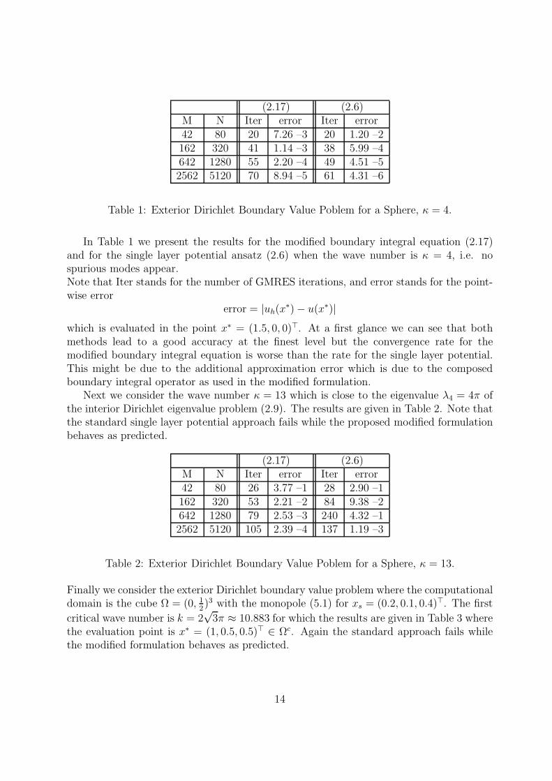
Table 1: Exterior Dirichlet Boundary Value Poblem for a Sphere, κ = 4.

In Table 1 we present the results for the modified boundary integral equation (2.17)and for the single layer potential ansatz (2.6) when the wave number is κ = 4, i.e. nospurious modes appear.Note that Iter stands for the number of GMRES iterations, and error stands for the point-wise error

error = |uh(x∗) − u(x∗)|

which is evaluated in the point x∗ = (1.5, 0, 0)⊤. At a first glance we can see that bothmethods lead to a good accuracy at the finest level but the convergence rate for themodified boundary integral equation is worse than the rate for the single layer potential.This might be due to the additional approximation error which is due to the composedboundary integral operator as used in the modified formulation.

Next we consider the wave number κ = 13 which is close to the eigenvalue λ4 = 4π ofthe interior Dirichlet eigenvalue problem (2.9). The results are given in Table 2. Note thatthe standard single layer potential approach fails while the proposed modified formulationbehaves as predicted.

(2.17) (2.6)M N Iter error Iter error42 80 26 3.77 –1 28 2.90 –1162 320 53 2.21 –2 84 9.38 –2642 1280 79 2.53 –3 240 4.32 –12562 5120 105 2.39 –4 137 1.19 –3

Table 2: Exterior Dirichlet Boundary Value Poblem for a Sphere, κ = 13.

Finally we consider the exterior Dirichlet boundary value problem where the computationaldomain is the cube Ω = (0, 1

2)3 with the monopole (5.1) for xs = (0.2, 0.1, 0.4)⊤. The first

critical wave number is k = 2√

3π ≈ 10.883 for which the results are given in Table 3 wherethe evaluation point is x∗ = (1, 0.5, 0.5)⊤ ∈ Ωc. Again the standard approach fails whilethe modified formulation behaves as predicted.

14

(2.17) (2.6)M N Iter error Iter error14 24 9 1.57 –1 9 1.94 –150 96 27 3.05 –3 27 2.82 –1

184 384 42 1.05 –3 42 4.93 –1770 1536 59 3.12 –4 59 2.32

3074 6144 73 1.38 –4 76 9.05 –1

Table 3: Exterior Dirichlet Boundary Value Poblem for a Cube, κ = 2√

3π.

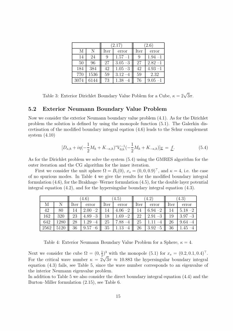
5.2 Exterior Neumann Boundary Value Problem

Now we consider the exterior Neumann boundary value problem (4.1). As for the Dirichletproblem the solution is defined by using the monopole function (5.1). The Galerkin dis-cretisation of the modified boundary integral eqation (4.6) leads to the Schur complementsystem (4.10)

[Dκ,h + iη(−1

2Mh +K−κ,h)

∗V −10,h (−1

2Mh +K−κ,h)]v = f. (5.4)

As for the Dirichlet problem we solve the system (5.4) using the GMRES algorithm for theouter iteration and the CG algorithm for the inner iteration.

First we consider the unit sphere Ω = B1(0), xs = (0, 0, 0.9)⊤, and κ = 4, i.e. the caseof no spurious modes. In Table 4 we give the results for the modified boundary integralformulation (4.6), for the Brakhage–Werner formulation (4.5), for the double layer potentialintegral equation (4.2), and for the hypersingular boundary integral equation (4.3).

(4.6) (4.5) (4.2) (4.3)M N Iter error Iter error Iter error Iter error42 80 14 2.00 –2 14 4.06 –2 14 6.94 –2 14 5.18 –2162 320 23 4.89 –3 18 1.69 –2 22 2.91 –3 19 3.97 –3642 1280 28 1.29 –4 25 7.88 –4 25 1.11 –4 26 9.64 –42562 5120 36 9.57 –6 35 1.13 –4 26 3.92 –5 36 1.45 –4

Table 4: Exterior Neumann Boundary Value Problem for a Sphere, κ = 4.

Next we consider the cube Ω = (0, 12)3 with the monopole (5.1) for xs = (0.2, 0.1, 0.4)⊤.

For the critical wave number κ = 2√

3π ≈ 10.883 the hypersingular boundary integralequation (4.3) fails, see Table 5, since the wave number corresponds to an eigenvalue ofthe interior Neumann eigenvalue problem.In addition to Table 5 we also consider the direct boundary integral equation (4.4) and theBurton–Miller formulation (2.15), see Table 6.

15

(4.6) (4.5) (4.2) (4.3)M N Iter error Iter error Iter error Iter error14 24 7 1.46 –1 7 3.13 –1 7 8.11 –1 7 2.90 –150 96 22 7.67 –3 19 9.61 –2 20 2.22 –1 19 8.10 –2194 384 29 2.43 –3 26 1.25 –2 30 1.45 –1 29 6.01 –2770 1536 36 3.80 –4 39 1.44 –3 35 7.05 –2 44 5.83 –23074 6144 50 5.56 –5 54 2.25 –4 37 3.56 –2 64 6.19 –2

Table 5: Exterior Neumann Boundary Value Problem for a Cube, κ = 2√

3π.

(4.4) (2.15)M N Iter error Iter error14 24 6 2.65 –1 6 2.85 –150 96 19 7.33 –2 19 7.95 –2194 384 29 1.11 –2 25 1.07 –2770 1536 44 2.58 –3 38 2.47 –33074 6144 64 6.35 –4 53 6.09 –4

Table 6: Neumann Boundary Value Problem for a Cube, κ = 2√

3π.

6 Conclusions

In this paper we have formulated and analyzed modified boundary element methods forthe Dirichlet and Neumann boundary value problems of the Helmholtz equation whichare stable for all wave numbers. In contrast to other existing approaches the proposedmethod relies on the use boundary integral operators which are already available in stan-dard boundary element methods. Therefore, the additional effort in the implementation isneglectible.

Open questions concern the construction of efficient preconditioned iterative solutionstrategies where also an optimal choice of the scaling parameter η ∈ R+ is crucial, see[1, 14, 15]. Note that the use of fast boundary element methods [11, 12, 18] will enable usto handle challenging applications.

Acknowledgements

We would like to thank Dr. M. Fischer and Dr. G. Of for providing us parts of their codes.This cooperation and further discussions are greatfully acknowledged.

16

References

[1] S. Amini. On the choice of the coupling parameter in boundary integral formulationsof the exterior acoustic problem. Appl. Anal., 35(1-4):75–92, 1990.

[2] S. Amini and D. T. Wilton. An investigation of boundary element methods for theexterior acoustic problem. Comput. Methods Appl. Mech. Engrg., 54(1):49–65, 1986.

[3] X. Antoine and M. Darbas. Alternative integral equations for the iterative solution ofacoustic scattering problems. Quart. J. Mech. Appl. Math., 58(1):107–128, 2005.

[4] W. Benthien and A. Schenck. Nonexistence and nonuniqueness problems associatedwith integral equation methods in acoustics. Comput. & Structures, 65(3):295–305,1997.

[5] H. Brakhage and P. Werner. Uber das Dirichletsche Aussenraumproblem fur dieHelmholtzsche Schwingungsgleichung. Arch. Math., 16:325–329, 1965.

[6] A. Buffa and R. Hiptmair. Regularized combined field integral equations. Numer.Math., 100(1):1–19, 2005.

[7] A. Buffa and S. Sauter. On the acoustic single layer potential: stabilization andFourier analysis. SIAM J. Sci. Comput., 28(5):1974–1999 (electronic), 2006.

[8] A. J. Burton and G. F. Miller. The application of integral equation methods to thenumerical solution of some exterior boundary-value problems. Proc. Roy. Soc. London.Ser. A, 323:201–210, 1971. A discussion on numerical analysis of partial differentialequations (1970).

[9] D. Colton and R. Kress. Inverse acoustic and electromagnetic scattering theory, vol-ume 93 of Applied Mathematical Sciences. Springer, Berlin, 1998.

[10] S. Engleder and O. Steinbach. Modified Boundary Integral Formulations for theHelmholtz Equation. J. Math. Anal. Appl., 331:396–407, 2007.

[11] M. Fischer. The Fast Multipole Boundary Element Method and its Application toStructure-Acoustic Field Interaction, 2004. Dissertation, Universitat Stuttgart.

[12] K. Giebermann. Schnelle Summationsverfahren zur numerischen Losung von Integral-gleichungen fur Streuprobleme im R

3, 1997. Dissertation, Fakultat fur Mathematik,Universitat Karlsruhe.

[13] R. E. Kleinman and G. F. Roach. Boundary integral equations for the three-dimensional Helmholtz equation. SIAM Rev., 16:214–236, 1974.

[14] R. Kress. Minimizing the condition number of boundary integral operators in acousticand electromagnetic scattering. Quart. J. Mech. Appl. Math., 38(2):323–341, 1985.

17

[15] R. Kress and W. T. Spassov. On the condition number of boundary integral operatorsfor the exterior Dirichlet problem for the Helmholtz equation. Numer. Math., 42(1):77–95, 1983.

[16] W. McLean. Strongly Elliptic Systems and Boundary Integral Equations. CambridgeUniversity Press, Cambridge, 2000.

[17] G. Of and O. Steinbach. A fast multipole boundary element method for a modifiedhypersingular boundary integral equation. Lect. Notes Appl. Comput. Mech., 12:163–169, 2003.

[18] S. Rjasanow and O. Steinbach. The Fast Solution of Boundary Integral Equations.Springer, New York, 2007.

[19] S. Sauter and C. Schwab. Randelementmethoden. Teubner, Stuttgart, Leipzig, Wies-baden, 2004.

[20] A. Schatz, V. Thomee, and W. Wendland. Mathematical theory of finite and boundaryelement methods, volume 15 of DMV Seminar. Birkhauser Verlag, Basel, 1990.

[21] H. A. Schenck. Improved integral formulation for acoustic radiation problems. J.Acoust. Soc. Am., 44:41–58, 1968.

[22] O. Steinbach. Numerical Approximation Methods for Elliptic Boundary Value Prob-lems. Finite and Boundary Elements. Springer, New York, 2007.

18

Erschienene Preprints ab Nummer 2006/1

2006/1 S. Engleder, O. Steinbach: Modified Boundary Integral Formulations for the Helm-holtz Equation.

2006/2 O. Steinbach (ed.): 2nd Austrian Numerical Analysis Day. Book of Abstracts.

2006/3 B. Muth, G. Of, P. Eberhard, O. Steinbach: Collision Detection for ComplicatedPolyhedra Using the Fast Multipole Method of Ray Crossing.

2006/4 G. Of, B. Schneider: Numerical Tests for the Recovery of the Gravity Field by FastBoundary Element Methods.

2006/5 U. Langer, O. Steinbach, W. L. Wendland (eds.): 4th Workshop on Fast BoundaryElement Methods in Industrial Applications. Book of Abstracts.

2006/6 O. Steinbach (ed.): Jahresbericht 2005/2006.

2006/7 G. Of: The All–floating BETI Method: Numerical Results.

2006/8 P. Urthaler, G. Of, O. Steinbach: Automatische Positionierung von FEM–Netzen.

2006/9 O. Steinbach: Challenges and Applications of Boundary Element Domain Decom-position Methods.

2006/10 S. Engleder: Stabilisierte Randintegralgleichungen fur aussere Randwertproblemeder Helmholtz–Gleichung

2007/1 M. Windisch: Modifizierte Randintegralgleichungen fur elektromagnetische Streu-probleme.

2007/2 M. Kaltenbacher, G. Of, O. Steinbach: Fast Multipole Boundary Element Methodfor Electrostatic Field Computations.

2007/3 G. Of, A. Schwaigkofler, O. Steinbach: Boundary integral equation methods forinverse problems in electrical engineering.

2007/4 S. Engleder, O. Steinbach: Stabilized Boundary Element Methods for ExteriorHelmholtz Problems

2007/5 O. Steinbach, G. Unger: A Boundary Element Method for the Dirichlet EigenvalueProblem of the Laplace Operator

2007/6 O. Steinbach, M. Windisch: Modified combined field integral equations for electro-magnetic scattering

2007/7 S. Gemmrich, N. Nigam, O. Steinbach: Boundary Integral Equations for theLaplace–Beltrami Operator.