
Running head: FROM ANOMALIES TO FORECASTS 1 From …
102
Running head: FROM ANOMALIES TO FORECASTS 1 From Anomalies to Forecasts: Toward a Descriptive Model of Decisions under Risk, under Ambiguity, and from Experience Ido Erev Technion and Warwick University Eyal Ert The Hebrew University of Jerusalem Ori Plonsky, Doron Cohen, and Oded Cohen Technion Author Note Ido Erev, Max Wertheimer Minerva Center for Cognitive Studies, Faculty of Industrial Engineering and Management, Technion and Warwick Business School, Warwick University; Eyal Ert, Department of Environmental Economics and Management, The Hebrew University of Jerusalem; Ori Plonsky, Doron Cohen, and Oded Cohen, Max Wertheimer Minerva Center for Cognitive Studies, Faculty of Industrial Engineering and Management, Technion. This research was supported by the I-CORE program of the Planning and Budgeting Committee and the Israel Science Foundation (grant no. 1821/12 for Ido Erev, and grant no. 1739/14 for Eyal Ert). We thank Alvin E. Roth, Asen Kochov, Eric Schulz, and Michael Sobolev for their useful comments. We also thank members of 25 teams for participation in the competition, and Shier Cohen-Amin, Shani Haviv, Liron Honen, and Yaara Nussinovitch for their help in data collection. Correspondence concerning this article should be addressed to Ido Erev, Max Wertheimer Minerva Center for Cognitive Studies, Faculty of Industrial Engineering and Management, Technion, Haifa, 3200003, Israel. E-mail: [email protected]
Transcript of Running head: FROM ANOMALIES TO FORECASTS 1 From …

Running head: FROM ANOMALIES TO FORECASTS 1
From Anomalies to Forecasts: Toward a Descriptive Model of Decisions under Risk, under
Ambiguity, and from Experience
Ido Erev
Technion and Warwick University
Eyal Ert
The Hebrew University of Jerusalem
Ori Plonsky, Doron Cohen, and Oded Cohen
Technion
Author Note
Ido Erev, Max Wertheimer Minerva Center for Cognitive Studies, Faculty of
Industrial Engineering and Management, Technion and Warwick Business School, Warwick
University; Eyal Ert, Department of Environmental Economics and Management, The
Hebrew University of Jerusalem; Ori Plonsky, Doron Cohen, and Oded Cohen, Max
Wertheimer Minerva Center for Cognitive Studies, Faculty of Industrial Engineering and
Management, Technion.
This research was supported by the I-CORE program of the Planning and Budgeting
Committee and the Israel Science Foundation (grant no. 1821/12 for Ido Erev, and grant no.
1739/14 for Eyal Ert). We thank Alvin E. Roth, Asen Kochov, Eric Schulz, and Michael
Sobolev for their useful comments. We also thank members of 25 teams for participation in
the competition, and Shier Cohen-Amin, Shani Haviv, Liron Honen, and Yaara Nussinovitch
for their help in data collection.
Correspondence concerning this article should be addressed to Ido Erev, Max
Wertheimer Minerva Center for Cognitive Studies, Faculty of Industrial Engineering and
Management, Technion, Haifa, 3200003, Israel. E-mail: [email protected]

FROM ANOMALIES TO FORECASTS 2
Abstract
Experimental studies of choice behavior document distinct, and sometimes contradictory,
deviations from maximization. For example, people tend to overweight rare events in one-
shot decisions under risk, and to exhibit the opposite bias when they rely on past experience.
The common explanations of these results assume that the contradicting anomalies reflect
situation-specific processes that involve the weighting of subjective values and the use of
simple heuristics. The current paper analyzes 14 choice anomalies that have been described
by different models, including the Allais, St. Petersburg, and Ellsberg paradoxes, and the
reflection effect. Next, it uses a choice prediction competition methodology to clarify the
interaction between the different anomalies. It focuses on decisions under risk (known payoff
distributions) and under ambiguity (unknown probabilities), with and without feedback
concerning the outcomes of past choices. The results demonstrate that it is not necessary to
assume situation-specific processes. The distinct anomalies can be captured by assuming high
sensitivity to the expected return and four additional tendencies: pessimism, bias toward
equal weighting, sensitivity to payoff sign, and an effort to minimize the probability of
immediate regret. Importantly, feedback increases sensitivity to probability of regret. Simple
abstractions of these assumptions, variants of the model Best Estimate And Sampling Tools
(BEAST), allow surprisingly accurate ex ante predictions of behavior. Unlike the popular
models, BEAST does not assume subjective weighting functions or cognitive shortcuts.
Rather, it assumes the use of sampling tools and reliance on small samples, in addition to the
estimation of the expected values.
Keywords: experience-description gap, out-of-sample predictions, St. Petersburg paradox,
prospect theory, reinforcement learning

FROM ANOMALIES TO FORECASTS 3
From Anomalies to Forecasts: Toward a Descriptive Model of Decisions under Risk, under
Ambiguity, and from Experience
Behavioral decision research is often criticized on the grounds that it highlights
interesting choice anomalies, but rarely supports clear forecasts. The main reason for the
difficulty in deriving clear predictions is that the classical anomalies are explained with
several descriptive models, and in many cases these models suggest contradicting behavioral
tendencies. Thus, it is not easy to predict the joint effect of the different tendencies. Nobel
laureate Alvin E. Roth (see Erev, Ert, Roth, et al., 2010) clarified this critique by asking
authors of papers that explain some of the anomalies to add a 1-800 (toll-free) phone number
and be ready to answer questions concerning the conditions under which their model applies.
In a seminal paper, Kahneman and Tversky (1979) attempted to address this problem
by first identifying four of the most important deviations from maximization (defined here as
violations of the assumption that people maximize expected return), replicating them in one
experimental paradigm, and finally proposing prospect theory, a model that captures the joint
effect of all these phenomena and thus allows clear predictions. Specifically, Kahneman and
Tversky replicated—and prospect theory addresses—the certainty effect (Allais paradox,
Allais, 1953; see Row 1 in Table 1), the reflection effect (following Markowitz, 1952; see
Row 2 in Table 1), overweighting of rare events (following Friedman & Savage, 1948; see
Row 3 in Table 1), and loss aversion (following Samuelson, 1963; see Row 4 in Table 1).
Importantly, the Kahneman and Tversky's replication, and prospect theory, focused on a very
specific choice environment: choice between gambles with “at most two non-zero outcomes”
(Kahneman & Tversky, 1979, p. 275).

FROM ANOMALIES TO FORECASTS 4
Table 1
Examples of Fourteen Phenomena and Their Replications in the Current Study
Classical Demonstration Current Replication
Phenomenon Problems %B Choice Problems %B Choice
Phenomena observed in studies of decisions without feedback
1. Certainty effect/Allais paradox (Kahneman & Tversky, 1979, following Allais, 1953)
A: 3000 with certainty
B: 4000, .8; 0 otherwise
A’: 3000, .25; 0 otherwise
B’: 4000, .20; 0 otherwise
20%
65%
A: 3 with certainty
B: 4, .8; 0 otherwise
Aʹ: 3, .25; 0 otherwise
Bʹ: 4, .20; 0 otherwise
42%
61%
2. Reflection effect (Kahneman & Tversky, 1979)
A: 3000 with certainty
B: 4000, .8; 0 otherwise
A’: −3000 with certainty
B’: −4000, .8; 0 otherwise
20%
92%
A: 3 with certainty
B: 4, .8; 0 otherwise
Aʹ: −3 with certainty
Bʹ: −4, .8; 0 otherwise
42%
49%
3. Over-weighting of rare events (Kahneman & Tversky, 1979)
A: 5 with certainty
B: 5000, .001; 0 otherwise
72%
A: 2 with certainty
B: 101, .01; 1 otherwise
55%
4. Loss aversion (Ert & Erev, 2013, following Kahneman & Tversky, 1979)
A: 0 with certainty
B: −100, .5; 100 otherwise
22%
A: 0 with certainty
B: −50, .5; 50 otherwise
34%
5. St. Petersburg paradox/risk aversion (Bernoulli, 1738/1954)
A fair coin will be flipped until it
comes up heads. The number of
flips will be denoted by the letter k.
The casino pays a gambler 2k.
What is the maximum amount of
money that you are willing to pay
for playing this game?
Modal
response:
less than 8
A: 9 with certainty
B: 2, 1/2; 4, 1/4; 8; 1/8; 16,
1/16; 32, 1/32; 64, 1/64;
128, 1/128; 256 otherwise
38%
6. Ellsberg paradox/Ambiguity aversion (Einhorn & Hogarth, 1986, following Ellsberg, 1961)
Urn K contains 50 red and 50 white
balls. Urn U contains 100 balls,
each either red or white, with
unknown proportions.
Choose between:
A: 100 if a ball drawn from K is
red; 0 otherwise
B: 100 if a ball drawn from U is
red; 0 otherwise
C: Indifference
47%
19%
34%
A: 10 with probability .5;
0 otherwise
B: 10 with probability ‘p’;
0 otherwise (‘p’ unknown
constant)
37%
7. Low magnitude eliminates loss aversion (Ert & Erev, 2013)
A: 0 with certainty
B: −10, .5; 10 otherwise
48%
A: 0 with certainty
B: −1, .5; 1 otherwise
49%

FROM ANOMALIES TO FORECASTS 5
Classical Demonstration Current Replication
Phenomenon Problems %B Choice Problems %B Choice
8. Break-even effect (Thaler & Johnson, 1990)
A: −2.25 with certainty
B: −4.50, .5; 0 otherwise
A': −7.50 with certainty
B': −5.25 .5; −9.75 otherwise
87%
77%
A: −1 with certainty
B: −2, .5; 0 otherwise
Aʹ: −2 with certainty
Bʹ: −3 .5; −1 otherwise
58%
48%
9. Get-something effect (Ert & Erev, 2013, following Payne, 2005)
A: 11, .5; 3 otherwise
B: 13, .5; 0 otherwise
A’: 12, .5; 4 otherwise
B’: 14, .5; 1 otherwise
21%
38%
A: 1 with certainty
B: 2, .5; 0 otherwise
Aʹ: 2 with certainty
Bʹ: 3 .5; 1 otherwise
35%
41%
10. Splitting effect (Birnbaum, 2008, following Tversky & Kahneman, 1986)
A: 96; .90; 14, .05; 12 .05
B: 96; .85; 90, .05; 12, .10
73%
A: 16 with certainty
B: 1, .6; 50, .4
Aʹ: 16 with certainty
Bʹ: 1, .6; 44, .1; 48, .1; 50, .2
49.9%
50.4%
Phenomena observed in studies of repeated decisions with feedback
11. Under-weighting of rare events (Barron & Erev, 2003)
A: 3 with certainty
B: 32, .1; 0 otherwise
A’: −3 with certainty
B’: −32, .1; 0 otherwise
32%
61%
A: 1 with certainty
B’: 20, .05; 0 otherwise
Aʹ: −1 with certainty
Bʹ: −20 .05; 0 otherwise
29%
64%
12. Reversed reflection (Barron & Erev, 2003)
A: 3 with certainty
B: 4, .8; 0 otherwise
A’: −3 with certainty
B’: −4, .8; 0 otherwise
63%
40%
A: 3 with certainty
B: 4, .8; 0 otherwise
Aʹ: −3, with certainty
Bʹ: −4, .8; 0 otherwise
65%
40%
13. Payoff variability effect (Erev & Haruvy, 2009, following Busemeyer & Townsend, 1993)
A: 0 with certainty
B: 1 with certainty
A’: 0 with certainty
B’: −9, .5; 11 otherwise
96%
58%
A: 2 with certainty
B: 3 with certainty
A': 6 if E; 0 otherwise
B': 9 if not E; 0 otherwise
P(E) = 0.5
100%
84%
14. Correlation effect (Grosskopf, Erev, & Yechiam, 2006, following Diederich & Busemeyer, 1999)
A: 150+N1 if E; 50+N1 otherwise
B: 160+N2 if E'; 60 +N2 otherwise
A': 150+N1 if E; 50+N1 otherwise
B': 160+N2 if E; 60 +N2 otherwise
Ni ~ N(0,20), P(E) = P(E') = .5
82%
98%
A: 6 if E; 0 otherwise
B: 9 if not E; 0 otherwise
A’: 6 if E; 0 otherwise
B’: 8 if E; 0 otherwise
P(E) = 0.5
84%
98%
Note. The notation x, p means payoff of x with probability p. In the classical demonstrations, choice rates are for
one-shot decisions in the no-feedback phenomena and for mean of the final 100 trials (of 200 or 400) in the
with-feedback phenomena. In current replications, choice rates are for five consecutive choices without
feedback in the no-feedback phenomena and for the last five trials (of 25) in the with-feedback phenomena.

FROM ANOMALIES TO FORECASTS 6
Tversky and Kahneman (1992; and see Wakker, 2010) presented a refined version of
prospect theory (cumulative prospect theory, CPT) that clarifies the assumed processes and
their relationship to the computations required to maximize expected value (EV). To
compute the EV of a prospect, the decision maker should weight each monetary outcome by
its objective probability. For example, the EV of a prospect that provides “4000 with
probability 0.8, 0 otherwise” is 4000∙(.8) + 0∙(.2) = 3200. CPT assumes modified weighting.
The subjective value of each outcome is weighted by its subjective weight. For example, the
attractiveness of the prospect “4000 with probability 0.8, 0 otherwise” under CPT is
V(4000)∙π(.8) + V(0)∙(1−π(0.8)), where V(∙) is a subjective value function that is assumed to
reflect diminishing sensitivity and loss aversion, and π(∙) is a subjective weighting function
that is assumed to reflect oversensitivity to extreme outcomes.
The success of prospect theory—and later of its successor CPT—has triggered three
lines of follow-up studies that attempt to reconcile this model with other choice anomalies.
One line of research (e.g., Rieger & Wang, 2006; Tversky & Bar-Hillel, 1983; Tversky &
Fox, 1995; Wakker, 2010) focuses on classical choice anomalies originally observed under
experimental paradigms not addressed by the original model: the St. Petersburg paradox
(Bernoulli, 1954; see Row 5 in Table 1) and the Ellsberg paradox (Ellsberg, 1961; see Row 6
in Table 1). This line of research suggests that extending prospect theory or CPT to address
these classical anomalies generally requires additional non-trivial assumptions and/or
parameters. For example, it is difficult to capture the four original anomalies and the St.
Petersburg paradox with one set of parameters (e.g., Blavatskyy, 2005; Rieger & Wang,
2006).
A second line of research focuses on newly-observed choice anomalies documented
within the limited setting of choice between simple fully described gambles, which prospect
theory was developed to address. These studies highlight new anomalies that emerge in this

FROM ANOMALIES TO FORECASTS 7
setting but cannot be captured with CPT. For example, Ert and Erev (2013; see Row 7 in
Table 1) showed that low stakes eliminate the tendency to exhibit loss aversion; Thaler and
Johnson (1990) documented a “break-even” effect (more risk seeking when only the risky
choice can prevent losses; see Row 8 in Table 1); Payne (2005) documented a “get-
something” effect (less risk seeking when only the safe prospect guarantees a gain; see Row 9
in Table 1); and Birnbaum (2008) documented a splitting effect (splitting a possible outcome
into two less desirable outcomes can increase its attractiveness; see Row 10 in Table 1).
Against the background of the difficulty in reconciling CPT with these new anomalies, an
alternative approach has suggested that some anomalies might be more naturally explained as
a reflection of simple heuristics rather than as a reflection of subjective weighting processes.
For example, the get-something effect can be the product of the use of a Pwin heuristic,
which implies choosing the option that maximizes the probability of gaining (e.g.,
Venkatraman, Payne, & Huettel, 2014). Brandstätter, Gigerenzer, and Hertwig (2006) show
that it is also possible to find a simple heuristic that can explain the anomalies that motivated
prospect theory in the first place (see Rows 1 to 4 in Table 1).
A third line of follow-up research focuses on the effects of experience. Thaler,
Tversky, Kahneman, and Schwartz (1997) and Fox and Tversky (1998) presented natural
generalizations of prospect theory to situations in which agents have to rely on their past
experience, but subsequent research (Hertwig, Barron, Weber, & Erev, 2004) highlights
robust phenomena that cannot be captured with these generalizations. This line of research
has proven to be particularly difficult to reconcile with prospect theory, as it questions the
generality of the very anomalies that motivate it. The availability of feedback was found to
reverse some of the anomalies considered above. The clearest examples for the effects of
feedback include underweighting of rare events (Barron & Erev, 2003; see Row 11 in Table
1), a reversed reflection effect (Barron & Erev, 2003; see Row 12 in Table 1), a payoff

FROM ANOMALIES TO FORECASTS 8
variability effect (Busemeyer & Townsend, 1993; see Row 13 in Table 1), and a correlation
effect (Diederich & Busemeyer, 1999; see Row 14 in Table 1). Once again, for
generalizations of prospect theory or CPT to capture anomalies in this line of research,
additional non-trivial assumptions are necessary (see, e.g., Fox & Hadar, 2006; Glöckner,
Hilbig, Henninger, & Fiedler, 2016). Congruently, the leading explanations of the
phenomena observed in decisions involving feedback assume a different underlying process,
according to which decision makers tend to rely on small samples of their past experiences
(Erev & Barron, 2005; Hertwig et al., 2004).
The different studies that aimed to develop descriptive models that capture subsets of
the 14 phenomena we have just described and are summarized in Table 1, have led to many
useful insights. However, they also suffer from a major shortcoming. Different modifications
of prospect theory and models that assume other processes address different well-studied
domains of problems. Thus, it is not clear how to use them outside the boundaries of these
domains. For example, according to Erev, Ert, Roth, et al. (2010), the best models that
capture behavior in decisions under risk assume very different processes than the best models
that capture behavior in repeated decisions with feedback. But which type of model should
we use if our goal is, for example, to design an incentive mechanism to be implemented in in-
vehicle data recorders aimed at promoting safe driving? The drivers of a car equipped with
such devices would be informed of the incentives and would also gain experience using the
system. In other words, which model should be used to predict the choice between fully
described gambles following a few trials with feedback? And what if the gambles include
many possible outcomes (as in the St. Petersburg paradox) or if one of these gambles is
ambiguous (as in the Ellsberg paradox)? The existing models shed only limited light on the
conditions that trigger different behavioral tendencies, so better understanding of these
conditions is required in order to address Roth’s 1-800 critique.

FROM ANOMALIES TO FORECASTS 9
The current research attempts to improve our understanding of the conditions that
trigger the different anomalies by extending the focus of the analysis. Rather than focusing on
a subset of the 14 anomalies presented in Table 1 (specifically, Kahneman & Tversky
focused on a subset of size 4), we try to capture all 14 anomalies with a single model. Unlike
the previous attempts to extend Kahneman and Tversky's (1979) analysis, discussed above,
we build on their method rather than on their model. Like Kahneman and Tversky (1979), we
start by trying to replicate the target anomalies in a single experimental paradigm, and then
develop a single model that captures the behavioral results.
The Problem of Overfitting and The Current Project
As noted above, previous research suggests that choice behavior is possibly affected
by three very different types of cognitive processes: processes that weigh subjective values
by subjective functions of their probabilities; those that assume simple heuristics; and those
that assume sampling from memory. It is also possible that one of these processes captures
behavior better than the others, but it requires making different assumptions in different
settings. An attempt to capture the interaction between several unobserved processes or to
identify the boundaries of the settings in which different assumptions are necessary involves
a high risk of overfitting the data. There are many feasible abstractions of the possible
processes and their interactions, and with so many degrees of freedom, it is not too difficult to
find abstractions that fit all 14 anomalies.
The current research takes four measures to reduce this risk. The most important
measure is the focus on predictions, rather than on fitting. Models are estimated here based
on one set of problems, and then compared based on their ability to predict the behavior in a
second, initially unobserved, set of problems. A second measure involves the replication of
the classical anomalies in one standard paradigm (Hertwig & Ortmann, 2001; like Kahneman
& Tversky, 1979). This replication eliminates the need to estimate paradigm-specific

FROM ANOMALIES TO FORECASTS 10
parameters. A third measure involves the study of randomly-selected problems (in addition to
the problems that demonstrate the interesting anomalies). This serves to increase the amount
of the data used to estimate and evaluate the models. A fourth measure involves the
organization of a choice prediction competition (see Arifovic, McKelvey, & Pevnitskaya,
2006; Erev, Ert, Roth, et al., 2010). The first three co-authors of the current paper (Erev, Ert
& Plonsky; hereinafter EEP) first presented the best model they could find, and then
challenged other researchers to find a better model. The competition methodology is expected
to reduce the risk of overfitting the data caused by focusing on a small set of models
considered by a small group of researchers. That is, rather than putting forth the set of
contender models themselves, EEP asked the research community to provide the contenders.
In the first part of the current project, EEP developed a “standard” paradigm (Hertwig
& Ortmann, 2001) and identified an 11-dimensional space of experimental tasks wide enough
to replicate all 14 behavioral phenomena described above and illustrated in Table 1. Next,
EEP conducted a replication study consisting of 30 carefully selected choice tasks. The
replication study shows that all 14 behavioral phenomena emerge in this 11-dimensional
space. Yet, their magnitude tends to be smaller than it was in the original demonstrations.
The second part of the current project includes a calibration study in which 60
additional problems, randomly selected from the same 11-dimensional space of tasks that
includes the replication problems, were investigated. The results clarify the robustness and
the boundaries of the distinct behavioral phenomena. Based on the results of these 90
problems (30 in the replication study and 60 in the calibration study), EEP developed a
“baseline” model that presents their best attempt to capture behavior in the wide space of
choice tasks. This model assumes that two components drive choice. The first is the option's
expected value (and not a weighting of subjective values, as modeled by EUT and CPT). The
second is the outcome of four distinct tendencies that are products of sampling “tools.”

FROM ANOMALIES TO FORECASTS 11
The paper concludes with the presentation of the choice prediction competition. The
organizers (EEP) posted the results of the first two experiments, as well as a description of
the baseline model, on the web (at http://departments.agri.huji.ac.il/cpc2015). EEP then
challenged other researchers (with emails to members of the popular scientific organizations
in psychology, decision science, behavioral economics, and machine learning) to develop a
better model. The competition focused on the prediction of the results of a third (“test”)
experimental study that was run after posting the baseline model. The call for participation in
the competition was posted in January 2015, and the competition study was run in April 2015
(its results were published only after the submission deadline in May 2015). A famous Danish
proverb (commonly attributed to Niels Bohr) states “it is difficult to make predictions, especially
about the future.” Running the competition study only after everyone submitted their models
ensured that the competition participants actually dealt with this difficulty of predicting the
future, and could not satisfy with fitting data that is already known.
Researchers from five continents responded to the prediction competition challenge,
submitting a total of 25 models. The submissions included three models that are variants of
prospect theory with situation-specific parameters, 14 models that are similar to the baseline
model and assume that behavior is driven by the expected return and four additional
behavioral tendencies, and seven models that do not try to directly abstract the underlying
process, but rely primarily on statistical methods (like machine learning algorithms). All 12
highest ranked submissions were variants of the baseline. The “prize” for the winners was co-
authorship of this paper; the last two authors (Cohen & Cohen) submitted the winning model.
Space of Choice Problems
The previous studies that demonstrated the behavioral phenomena summarized in
Table 1 used diverse experimental paradigms. For example, the Allais paradox/certainty
effect was originally demonstrated in studies that examined choice among fully described

FROM ANOMALIES TO FORECASTS 12
gambles (Allais, 1953; Kahneman & Tversky, 1979), while the Ellsberg paradox was
originally demonstrated in studies that focused on bets on the color of a ball drawn from
partially described urns (Einhorn & Hogarth, 1986; Ellsberg, 1961). In addition, within the
same experimental paradigm, different payoff distributions give rise to different behavioral
phenomena. In other words, the differences among the various demonstrations of the
behavioral phenomena in Table 1 involve multiple dimensions, such as the framing
manipulation, the number of possible outcomes, and the shape of the payoff distributions.
Thus, it is possible to think of the classical demonstrations in Table 1 as points in a
multidimensional space of “choice tasks.” This abstraction clarifies the 1-800 critique against
behavioral decision research. The critique rests on the observation that the leading models
were designed to capture specific sections (typically involving interesting anomalies) in this
space of choice problems. Thus, different models address different points in the space, and
the models’ boundaries are not always clear. Consequently, it is not clear which model should
be used to predict behavior in a new choice task.
Our research attempts to address this critique by facilitating the study of a space of
choice tasks wide enough to give rise to all 14 phenomena summarized in Table 1. We began
by trying to identify the critical dimensions of this multidimensional space. Our effort
suggests that the main properties of the problems in Table 1 include at least 11 dimensions.
Nine of the 11 dimensions can be described as parameters of the payoff distributions. These
parameters include: LA, HA, pHA, LB, HB, pHB, LotNum, LotShape, and Corr. In particular,
each problem in the space is a choice between Option A, which provides HA with probability
pHA or LA otherwise (with probability 1 − pHA), and Option B, which provides a lottery (that
has an expected value of HB) with probability pHB, and provides LB otherwise (with
probability 1 − pHB). The distribution of the lottery around its expected value (HB) is
determined by the parameters LotNum (which defines the number of possible outcomes in the

FROM ANOMALIES TO FORECASTS 13
lottery) and LotShape (which defines whether the distribution is symmetric around its mean,
right-skewed, left-skewed, or undefined if LotNum = 1), as explained in Appendix A. The
Corr parameter determines whether there is a correlation (positive, negative, or zero) between
the payoffs of the two options.
The tenth parameter, Ambiguity (Amb), captures the precision of the initial
information the decision maker receives concerning the probabilities of the possible
outcomes in Option B. We focus on the two extreme cases: Amb = 1 implies no initial
information concerning these probabilities (they are described with undisclosed fixed
parameters), and Amb = 0 implies complete information and no ambiguity (as in Allais, 1953;
Kahneman & Tversky, 1979).
The eleventh dimension in the space is the amount of feedback the decision maker
receives after making a decision. As Table 1 shows, some phenomena emerge in decisions
without feedback (i.e., decisions from description), and other phenomena emerge when the
decision maker can rely on feedback (i.e., decisions from experience). We studied this
dimension within problem. That is, decision makers faced each problem first without
feedback, and then with full feedback (i.e., realization of the obtained and forgone outcomes
following each choice).
The main hypothesis of the replication exercise described below is that this 11-
dimensional space is sufficiently large to give rise to all the behavioral phenomena from
Table 1.1 That is, we examine whether all these phenomena can be replicated within the
1 Notice that the 11 dimensions were selected to ensure that certain value combinations would imply
choice tasks likely to give rise to the 14 phenomena. The first six dimensions are necessary to allow for the
Allais pattern. The LotNum and LotShape dimensions are necessary to allow for the St. Petersburg paradox and
splitting pattern. The Ambiguity dimension is necessary to allow for the Ellsberg paradox. The correlation
dimension is necessary to allow for the regret/correlation effect. And the feedback dimension is necessary to
allow the experience phenomena. We also had to limit the range of values that each of the 11 dimensions could
take, which inevitably added technical constraints to the space of problems we actually studied. For example,

FROM ANOMALIES TO FORECASTS 14
abstract framing of choice between gambles (used, e.g., by Allais, 1953; Kahneman &
Tversky, 1979), although some were originally demonstrated in different experimental
paradigms, such as urns or coin-tosses. To facilitate this examination, we considered, in
addition to the 11 dimensions, two framing manipulations (“coin-toss” and “accept/reject”)
that were suggested by previous studies as important to two of the phenomena (to the St.
Petersburg paradox, see Erev, Glozman, & Hertwig, 2008; and to loss aversion, see Ert &
Erev, 2013, respectively). Under the “accept/reject framing,” Option B is presented as the
acceptance of a gamble, and Option A as the status quo (rejecting the gamble). Under the
“coin-toss framing,” the lottery is described as a coin-toss game similarly to Bernoulli’s
description (1738/1954) in his illustration of the St. Petersburg paradox. Hence, each of the
30 problems studied in our replication study (Appendix B) is uniquely defined by specific
values in each of the 10 dimensions described above in addition to a framing manipulation
(and, as noted, the eleventh dimension, feedback, is studied within the problems).
Initially, we also planned to consider the role of the difference between hypothetical
and real monetary payoffs. We chose to drop this dimension and focus on real payoffs,
following a pilot study in which more than 30% of the subjects preferred the hypothetical
gamble “−1000 with probability .1; +1 otherwise” over the status quo (zero with certainty).
This pilot study reminded us that the main effect of the study of hypothetical problems is an
increase in choice variance (Camerer & Hogarth, 1999).
Replications of Behavioral Phenomena
The current investigation was designed to undertake the following objectives: (a) to
explore whether the current 11-dimensional space is wide enough to replicate the 14 choice
the manner in which the lottery parameters define its distribution limits the possible lottery distributions in the
space (see Appendix A). Hence, the genuine hypothesis of the replication study is that even the limited 11-
dimensional space is sufficiently large to replicate all the classical phenomena from Table 1.

FROM ANOMALIES TO FORECASTS 15
phenomena summarized on the left-hand side of Table 1; (b) to clarify the boundaries and
relative importance of these phenomena; and (c) to test the robustness of two of the
phenomena to certain framing manipulations, which, according to previous research, matter.
To achieve these goals, we studied the 30 choice problems detailed in Appendix B.
Method
One hundred and twenty five students (63 male, MAge = 25.5) participated in the
experimental condition of the replication study, sixty at the Hebrew University of Jerusalem
(HU), and sixty-five at the Technion. Each participant faced each of the 30 decision problems
presented in Appendix B for 25 trials (i.e. each participant made 750 decisions). The order of
the 30 problems was random. Participants were told that they were going to play several
games, each for several trials, and their task in each trial was to choose one of the two options
on the screen for real money. The participants were also told that at the end of the study, one
of the trials would be randomly selected and that their obtained outcome in that trial would be
realized as their payoff (see examples of the experimental screen and a translation of the
instructions in Appendix C). Notice that this payment rule excludes potential “wealth
effects.” It implies that the participants could not “build portfolios,” e.g., by taking risks in
some trials and compensating for losses in others. Furthermore, both rational considerations
and the isolation effect (Kahneman & Tversky, 1979) imply independence between the
choices in the problems without ambiguity.
In the first five trials of each problem, the participants did not receive feedback after
each choice, so they had to rely solely on the description of the payoff distributions. Starting
at Trial 6, participants were provided with full feedback (the outcomes of each prospect) after
each choice; that is, in the last 19 trials, the participants could rely on the description of the

FROM ANOMALIES TO FORECASTS 16
payoff distributions and on feedback concerning the outcomes of previous trials.2 The final
payoff (including show-up fee) ranged from 10 to 110 shekels (M = 41.9, approximately
$11).3
In addition to the experimental condition, we ran two control conditions that used the
same participant recruitment and incentive methods as the main condition. The first, referred
to as “Single Choice”, used Kahneman and Tversky's (1979) paradigm. Each of 60
participants faced each of the 30 problems only once and without any feedback. The second
control, referred to as “FB from 1st” was identical to the main replication study with except
that all choices, from the very first trial, were followed by feedback. This control condition
included 29 participants. The results of both conditions are reported in the Control Conditions
and Robustness Checks section.
Results and Discussion
The main results of the experimental condition, the mean choice rates of Option B per
block of five trials and by feedback type (i.e., no-FB or with-FB) for each of the 30 problems
2 In addition, we compared two order conditions in a between-subject design. Sixty participants (30 in
each location) were assigned to the “by problem” (ByProb) order: they faced each problem for one sequence of
25 trials before facing the next problem. The other participants were assigned to the “by feedback” (ByFB)
order condition. This condition was identical to the ByProb condition, with one exception: the participants first
performed the five no-feedback trials in each of the 30 problems (in one sequence of 150 trials), and then faced
the remaining 20 trials with feedback of each problem (in one sequence of 600 trials, and in the same order of
problems they played in the no-feedback trials). Our analyses suggested almost no differences between the two
conditions, therefore we chose to focus on the choice patterns across conditions, and report these subtle
differences in the section Effects of Location and Order.
3 The show-up fee was determined for each participant individually such that the minimal possible
compensation for the experiment was 10 shekels. This was the maximum between 30 shekels and the sum of 10
shekels and the maximal possible loss in the problem that was randomly selected to determine the payoff. For
example, if Problem 12 was selected, the show-up fee was 60 shekels, but if Problem 1 was selected the show-
up fee was 30 Shekels. This procedure was never disclosed to participants and they only knew in advance their
expected total payoff. Specifically, there was no deception.

FROM ANOMALIES TO FORECASTS 17
are presented in Appendix B. The raw data (nearly 94,000 lines) is available online (see
http://departments.agri.huji.ac.il/cpc2015). In short, the results show that (a) all the 14
phenomena described in Table 1 emerge in our setting, but most description phenomena are
eliminated or even reversed after few trials with feedback; and (b) feedback increases
maximization when the best option leads to the best payoff in most trials, but can impair
maximization when this condition does not hold. Below we clarify the implications of the
results for the 14 behavioral phenomena summarized in Table 1.
The Allais paradox/certainty effect. The Allais paradox (Allais, 1953) is probably
the clearest and most influential counterexample to expected utility theory (Von Neumann &
Morgenstern, 1944). Kahneman and Tversky (1979) show that the psychological tendency
that underlies this paradox can be described as a certainty effect: safer alternatives are more
attractive when they provide gain with certainty. Figure 1 summarizes our investigation of
this effect using variants of the problems used by Kahneman and Tversky (Row 1 in Table 1)
to replicate Allais’ common ratio version of the paradox. Analysis of Block 1 (first 5 trials,
without feedback, or “no-FB”) shows the robustness of the certainty effect in decisions from
description. The safer prospect (A) was more attractive in Problem 1 when it provided a
positive payoff with certainty (A-rate of 58%, B-rate of 42%, SD = 0.42), than in Problem 2
when it involved some uncertainty (A-rate of 39%, B-rate of 61%, SD = 0.44). The difference
between the two rates is significant, t(124) = −3.69, p < .001.4 However, feedback reduced
this difference. The difference between the two problems across the four with-FB blocks (B-
rate of 60%, SD = 0.37 in Problem 1, and B-rate of 62%, SD = 0.39 in Problem 2) is
insignificant: t(124) = −0.59.
4 We report significance tests to clarify the robustness of each finding in our setting, and use a weaker
criterion to define replication. A phenomenon is considered to be “replicated” if the observed choice rates are in
the predicted direction.

FROM ANOMALIES TO FORECASTS 18
Prob. Option A Option B
1 (3, 1) (4, .8; 0)
2 (3, .25; 0) (4, .2; 0)
Figure 1. Problems That Test the Allais Paradox/Certainty Effect in the Replication Study. The notation
(x, p; y) refers to a prospect that yields a payoff of x with probability p and y otherwise. Option B’s choice
proportions are shown in five blocks of five trials each (Block 1: “no-FB,” Blocks 2–5: “with-FB”). The
experimental results are given with 95% CI for the mean. (The right-hand plot presents the prediction of the
baseline model described below).
The reflection and reversed reflection effects. A comparison of Problem 3 and
Problem 4 in Figure 2 demonstrates the reflection effect (Kahneman & Tversky, 1979, and
Row 2 in Table 1) in the no-FB block: risk aversion in the gain domain (B-rate of 35%,
SD = 0.42 in Problem 4) and risk seeking in the loss domain (B-rate of 58%, SD = 0.42 in
Problem 3). The difference is significant, t(124) = −4.99, p < .001. Feedback reduces this
effect. The B-rate across the four with-FB blocks (2 to 5) is 52% (SD = 0.37) in Problem 4
and 59% (SD = 0.35) in Problem 3. This difference is insignificant, t(124) = −1.59.
A comparison of Problem 1 with Problem 5 reveals a weaker indication of the
reflection effect. The results in the no-FB block show risk aversion in the gain domain (B-rate
of 42%, SD = 0.42 in Problem 1) and risk neutrality in the loss domain (B-rate of 49%,
SD = 0.42 in Problem 5); the difference is insignificant, t(124) = −1.24. Feedback reverses
the results and leads to lower risk-taking rate in the loss domain (B-rate of 40%, SD = 0.37 in
Problem 5) than in the gain domain (B-rate of 60%, SD = 0.37 in Problem 1). This reversed
reflection pattern (Barron & Erev, 2003; see Row 12 in Table 1) across the four with-FB
blocks, which suggests learning to maximize EV, is significant, t(124) = 3.90, p < .001.
1 2 3 4 5
Block
Model
0.00
0.25
0.50
0.75
1.00
1 2 3 4 5
P(B
)
Block
Experimental
0.00
0.25
0.50
0.75
1.00
1 2 3 4 5P
(B)
Block
Experimental
1: 3 or (4, .8; 0)
2: (3, .25; 0) or (4, .2; 0)
FROM ANOMALIES TO FORECASTS 19
Prob. Option A Option B
3 (−1, 1) (−2, .5; 0)
4 (1, 1) (2, .5; 0)
Prob. Option A Option B
5 (−3, 1) (−4, .8; 0)
1 (3, 1) (4, .8; 0)
Figure 2. Problems That Test the Reflection Effect in the Replication Study. The notation (x, p; y) refers to a
prospect that yields a payoff of x with probability p and y otherwise. Option B’s choice proportions are shown
in five blocks of five trials each (Block 1: “no-FB,” Blocks 2–5: “with-FB”). The experimental results are
given with 95% CI for the mean.
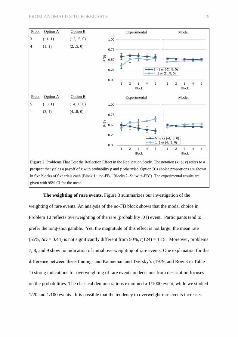
The weighting of rare events. Figure 3 summarizes our investigation of the
weighting of rare events. An analysis of the no-FB block shows that the modal choice in
Problem 10 reflects overweighting of the rare (probability .01) event. Participants tend to
prefer the long-shot gamble. Yet, the magnitude of this effect is not large; the mean rate
(55%, SD = 0.44) is not significantly different from 50%, t(124) = 1.15. Moreover, problems
7, 8, and 9 show no indication of initial overweighting of rare events. One explanation for the
difference between these findings and Kahneman and Tversky’s (1979, and Row 3 in Table
1) strong indications for overweighting of rare events in decisions from description focuses
on the probabilities. The classical demonstrations examined a 1/1000 event, while we studied
1/20 and 1/100 events. It is possible that the tendency to overweight rare events increases
1 2 3 4 5
Block
Model
0.00
0.25
0.50
0.75
1.00
1 2 3 4 5
P(B
)
Block
Experimental
0.00
0.25
0.50
0.75
1.00
1 2 3 4 5
P(B
)
Block
Experimental
3: -1 or (-2, .5; 0)
4: 1 or (2, .5; 0)
1 2 3 4 5
Block
Model
0.00
0.25
0.50
0.75
1.00
1 2 3 4 5
P(B
)
Block
Experimental
0.00
0.25
0.50
0.75
1.00
1 2 3 4 5
P(B
)
Block
Experimental
5: -3 or (-4, .8; 0)
1: 3 or (4, .8; 0)

FROM ANOMALIES TO FORECASTS 20
with their rarity. This explanation is supported by the observation that our results for the
positive rare outcomes reveal higher B-rate in the 1/100 case (mean of 51% in Problems 9
and 10, SD = 0.38) than in the 1/20 case (B-rate of 39%, SD = 0.43, in Problem 8). This
difference is significant, t(124) = 3.32, p = .001.
Prob. Option A Option B
7 (−1, 1) (−20, .05; 0)
8 (1, 1) (20, .05; 0)
9 (1, 1) (100, .01; 0)
10 (2, 1) (101, .01; 1)
Prob. Option A Option B
11 (19, 1) (−20, .1; 20)
Figure 3. Problems That Test the Weighting of Rare Events in the Replication Study. The notation (x, p; y)
refers to a prospect that yields a payoff of x with probability p and y otherwise. Option B’s choice proportions
are shown in five blocks of five trials each (Block 1: “no-FB,” Blocks 2-5: “with-FB”). The experimental
results are given with 95% CI for the mean.
Another explanation for the weaker indication of overweighting of rare events in our
no-FB block involves the possibility that the expectation that choice will be repeated (in the
current paradigm) reduces the weighting of rare events. An experiment that evaluates (and
rejects) this “expected repetitions” hypothesis is presented in the section Control Conditions
and Robustness Checks below.
1 2 3 4 5
Block
Model
0.00
0.25
0.50
0.75
1.00
1 2 3 4 5
P(B
)
Block
Experimental
0.00
0.25
0.50
0.75
1.00
1 2 3 4 5
P(B
)
Block
Experimental
7: -1 or (-20, .05; 0) 9: 1 or (100, .01; 0)
8: 1 or (20, .05; 0) 10: -1 or (101, .01; 1)
1 2 3 4 5
Block
Model
0.00
0.25
0.50
0.75
1.00
1 2 3 4 5
P(B
)
Block
Experimental
0.00
0.25
0.50
0.75
1.00
1 2 3 4 5P(B
)
Block
Experimental
11: 19 or (-20, .1; 20)

FROM ANOMALIES TO FORECASTS 21
Figure 3 also shows that the emergence of underweighting of rare events in decisions
with feedback is robust (Barron & Erev, 2003; Lejarraga & Gonzalez, 2011; and see Row 11
in Table 1). Experience reduces sensitivity to the rare event in all five problems. In the four
equal expected value problems (7, 8, 9, and 10), the choice rate following feedback reflects a
clear indication of underweighting of rare events: the choice rate of the prospect that leads to
the best payoff most of the time is 63% (SD = 0.37), 67% (SD = 0.39), 61% (SD = 0.42), and
57% (SD = 0.44) in problems 7, 8, 9, and 10 respectively (and all four values are significantly
greater than 50%, t(124) = 3.82, 4.77, 2.90, 1.72 respectively). Problem 11 highlights one
boundary of the underweighting of rare events. When the difference in expected value is
sufficiently large (19 versus 16), experience does not eliminate the tendency to prefer the
high expected value option over the risky alternative that leads to better payoff most of the
time (90% of the trials).
Loss aversion and the magnitude effect. The loss aversion hypothesis implies a
preference of the status quo over a symmetric fair gamble (e.g., a gamble that provides equal
probability of winning or losing x, Row 4 in Table 1). Figure 4 summarizes our investigation
of this hypothesis. Evaluation of the no-FB block in Problem 12 shows that the status quo
was preferred over equal chances to win or lose 50 in 66% (SD = 0.43, significantly more
than 50%, t(124) = 4.25, p < .001) of the cases. Problem 13 focuses on the same objective
task as Problem 12, with a different framing. The results show that in the current setting, the
difference between the accept/reject and the abstract framing is small: 64% (SD = 0.42,
significantly more than 50%, t(124) = 3.66, p < .001) of the choices reflect rejection of the
gamble in problem 13, similar to the rates observed in problem 12.5 Problem 14 replicates
5 Ert and Erev (2008, 2013) observed stronger support for loss aversion in the accept/reject framing
manipulation than in the abstract presentation. We believe that the lack of difference here reflects the fact that
our subjects were faced with many abstract problems, and this experience eliminated the format effect.

FROM ANOMALIES TO FORECASTS 22
the finding that low stakes eliminate the initial loss aversion bias (Ert & Erev, 2013; Harinck,
Van Dijk, Van Beest, & Mersmann, 2007; and see Row 5 in Table 1); the gamble was
selected in 49% (SD = 0.44) of the cases. The difference between problems 14 and 12 in the
no-FB block is significant, t(124) = −3.64, p < .001. The results for the last four blocks show
that feedback eliminated the magnitude effect, but not the general tendency to select the
status quo over the fair gamble.
Prob. Option A Option B
12 (0, 1) (50, .5; −50)
13 Reject B Accept a game
that gives equal
chances to win or
lose 50.
14 (0, 1) (1, .5; −1)
Prob. Option A Option B
15 (7, 1) (50, .5; 1)
16 (7, 1) (50, .5; −1)
17 (30, 1) (50, .5; 1)
18 (30, 1) (50, .5; −1)
Figure 4. Problems That Test Loss Aversion and Magnitude Effects in the Replication Study. The notation
(x, p; y) refers to a prospect that yields a payoff of x with probability p and y otherwise. Option B’s choice
proportions are shown in five blocks of five trials each (Block 1: “no-FB,” Blocks 2–5: “with-FB”). The
experimental results are given with 95% CI for the mean.
We added Problems 15, 16, 17, and 18 (lower panel in Figure 4) to study one
boundary of loss aversion, the observation that the addition of small losses to a dominant
(EV-wise) option can increase its attractiveness (Yechiam & Hochman, 2013). Our results do
1 2 3 4 5
Block
Model
0.00
0.25
0.50
0.75
1.00
1 2 3 4 5
P(B
)
Block
Experimental
0.00
0.25
0.50
0.75
1.00
1 2 3 4 5P(B
)
Block
Experimental
12: 0 or (50, .5; -50) 14: 0 or (1, .5; -1)
13: 0 or (50, .5; -50) Acc./Rej.
1 2 3 4 5
Block
Model
0.00
0.25
0.50
0.75
1.00
1 2 3 4 5
P(B
)
Block
Experimental
0.00
0.25
0.50
0.75
1.00
1 2 3 4 5
P(B
)
Block
Experimental
15: 7 or (50, .5; 1) 16: 7 or (50, .5; -1)
17: 30 or (50, .5; 1) 18: 30 or (50, .5; -1)

FROM ANOMALIES TO FORECASTS 23
not reveal this so-called “loss attention” pattern. Rather, they show similar sensitivity to the
expected values in all cases.
St. Petersburg paradox. Our experimental paradigm differs from the St. Petersburg
problem (Row 5 in Table 1) in many ways. Most importantly, we study choice rather than
bidding, and avoid the study of hypothetical tasks (and for that reason cannot examine a
problem with unbounded payoffs). Nevertheless, the robustness of the main behavioral
tendency demonstrated by the St. Petersburg paradox, risk aversion in the gain domain, can
be examined in our setting. Figure 5 summarizes our investigation. We studied two framings
of a bounded variant of the St. Petersburg problem. In Problem 19, the participants were
asked to choose between 9 with certainty, and a coin-toss game with the same expected
value. In Problem 20, the game’s possible outcomes and their objective probabilities were
listed on the screen. The results reveal a tendency to avoid the game that was slightly
increased by experience. The B-rates in the no-FB Block were 36% (SD = 0.42), and 38%
(SD = 0.43) in the “coin-toss” (St. Petersburg) and the “abstract” variants respectively. Both
rates are significantly lower than 50%, t(124) = −3.61 and −3.22, both p < .001. In addition,
the results across all five blocks show slightly lower B-rates in the coin format (34% vs.
37%). This difference is in the direction of the mere presentation hypothesis suggested by
Erev, Glozman, and Hertwig (2008), but the difference in the current setting is insignificant.

FROM ANOMALIES TO FORECASTS 24
Prob. Option A Option B
19 (9, 1) A fair coin will be
flipped until it comes
up heads but no more
than 8 times. Denote
the number of heads
with k. You get 2k.
20 (9, 1) (2, 1/2; 4, 1/4; 8, 1/8;
16, 1/16; 32, 1/32;
64, 1/64; 128, 1/128;
256)
Figure 5. Problems That Test the St. Petersburg Paradox in the Replication Study. The notation (x1, p1;
x2, p2; …; y) refers to a prospect that yields a payoff of x1 with probability p1, a payoff of x2 with probability
p2, …, and y otherwise. Option B’s choice proportions are shown in five blocks of five trials each (Block 1:
“no-FB,” Blocks 2–5: “with-FB”). The experimental results are given with 95% CI for the mean.
Ambiguity aversion/Ellsberg paradox. Ellsberg (1961, see Row 6 in Table 1) shows
a violation of subjective expected utility theory that can be described as an indication of
ambiguity aversion. Figure 6 summarizes our analysis of this phenomenon. The first block in
Problem 21 reveals ambiguity aversion: the typical choice (63%, SD = 0.41) favors the
prospect “10, .5; 0” over the ambiguous prospect “10 or 0 with unknown probabilities.” This
value is significantly greater than 50%, t(124) = 3.49, p < .001. Problem 22 reveals that
when gaining in the non-ambiguous option (A) occurs with low probability, people favor the
ambiguous option (ambiguity rate of 82%, SD = 0.30). Problem 23 shows a strong tendency
to avoid the ambiguous option when gaining in the non-ambiguous option is associated with
high probability (ambiguity rate of 15%, SD = 0.30). Both rates are significantly different
from 0.5, t(124) = 12.0 and −13.1, both p < .001, and are in line with previous findings of
studies in decisions in uncertain settings without feedback (e.g., Camerer & Weber, 1992).
Evaluation of the effect of experience reveals that feedback eliminates these attitudes towards
1 2 3 4 5
Block
Model
0.00
0.25
0.50
0.75
1.00
1 2 3 4 5
P(B
)
Block
Experimental
0.00
0.25
0.50
0.75
1.00
1 2 3 4 5P(B
)
Block
Experimental
19: Coin-toss frame
20: Abstract frame

FROM ANOMALIES TO FORECASTS 25
ambiguity (see Ert & Trautmann, 2014, for similar findings).6 The average choice rate of the
ambiguous option over the four with-FB blocks in these problems was 49%.
Prob. Option A Option B
21 (10, .5; 0) (10, p; 0)
p = .5 unknown
22 (10, .1; 0) (10, p; 0)
p = .1 unknown
23 (10, .9; 0) (10, p; 0)
p = .9 unknown
Figure 6. Problems that Test Ambiguity Attitudes in the Replication Study. The notation (x, p; y) refers to a
prospect that yields a payoff of x with probability p and y otherwise. In these problems, the probabilities of the
outcomes in Option B are undisclosed to participants (an ambiguous problem). Option B’s choice proportions
are shown in five blocks of five trials each (Block 1: “no-FB,” Blocks 2–5: “with-FB”). The experimental
results are given with 95% CI for the mean.
The break-even effect. Thaler and Johnson (1990, see Row 8 in Table 1) noticed that
people are more likely to take a risk in the loss domain when this risk can cover all their
losses and lead to a break-even outcome. The results, summarized in Figure 7, document the
break-even effect in the no-FB block. Our participants took significantly more risk in
Problem 3 (B-rate of 58%, SD = 0.42) and Problem 5 (B-rate 49%, SD = 0.42) when the risk
could eliminate the loss, than in Problem 24 (B-rate of 48%, SD = 0.44) and Problem 6 (B-
rate 38%, SD = 0.42) when the loss could not be avoided, t(124) = −2.01, p = .047 and
t(124) = −2.12, p = .036 respectively. Feedback did not eliminate this difference in the first
pair (3 and 24), but did eliminate it in the second (5 and 6). The B-rates over the four with-FB
blocks are 59% (SD = 0.35) in Problem 3 and 48% (SD = 0.37) in Problem 24, and the
6 Note that the description informed the subjects that the probabilities are fixed throughout the choice
task. Thus, the outcome observed in the early trials reduces the objective ambiguity. As previously noted (e.g.,
Epstein & Schneider, 2007; Maccheroni & Marinacci, 2005) there are situations, which go beyond the scope of
our space (e.g., when the probabilities can change), in which experience cannot eliminate ambiguity.
1 2 3 4 5
Block
Model
0.00
0.25
0.50
0.75
1.00
1 2 3 4 5P
(B)
Block
Experimental
0.00
0.25
0.50
0.75
1.00
1 2 3 4 5
P(B
)
Block
Experimental
21: (10, .5; 0) or (10, p; 0)22: (10, .1; 0) or (10, p; 0)23: (10, .9; 0) or (10, p; 0)

FROM ANOMALIES TO FORECASTS 26
difference is significant, t(124) = −2.76, p = .007. However, in both Problems 5 and 6, the B-
rates over the four with-FB blocks are 41%. The elimination of the break-even effect in the
latter case can be a reflection of an emergence, with feedback, of underweighting of the
relatively rare (20%) attractive no-loss outcome in Problem 5.
Prob. Option A Option B
3 (−1, 1) (−2, .5; 0)
24 (−2, 1) (−3, .5; −1)
Prob. Option A Option B
5 (−3, 1) (−4, .8; 0)
6 (−3, .25; 0) (−4, .2; 0)
Figure 7. Problems That Test the Break-Even Effect in the Replication Study. The notation (x, p; y) refers to a
prospect that yields a payoff of x with probability p and y otherwise. Option B’s choice proportions are shown
in five blocks of five trials each (Block 1: “no-FB,” Blocks 2–5: “with-FB”). The experimental results are
given with 95% CI for the mean.
The get-something effect. Payne (2005) shows that people are more likely to take
action that increases the probability of positive outcome than action that does not affect this
probability (Row 9 in Table 1). Our analysis of this tendency, summarized in Figure 8,
focuses on the comparison of Problem 4 with Problem 25 and the comparison of Problem 9
with Problem 10. Both comparisons reveal that in the no-FB block, our participants took less
risk when only the safer prospect (A) guaranteed a gain (B-rate of 35%, SD = 0.42 in
1 2 3 4 5
Block
Model
0.00
0.25
0.50
0.75
1.00
1 2 3 4 5
P(B
)
Block
Experimental0.00
0.25
0.50
0.75
1.00
1 2 3 4 5P(B
)
Block
Experimental
3: -1 or (-2, .5; 0)24: -2 or (-3, .5; -1)
1 2 3 4 5
Block
Model
0.00
0.25
0.50
0.75
1.00
1 2 3 4 5
P(B
)
Block
Experimental0.00
0.25
0.50
0.75
1.00
1 2 3 4 5
P(B
)
Block
Experimental
5: -3 or (-4, .8; 0)
6: (-3, .25; 0) or (-4, .2; 0)

FROM ANOMALIES TO FORECASTS 27
Problem 4, and B-rate of 47% SD = 0.44 in Problem 9) than they did in problems in which
both options guaranteed a gain (B-rate of 41%, SD = 0.44 in Problem 25, and B-rate of 55%,
SD = 0.44 in Problem 10). The effect is not large, but the difference between the two pairs is
significant in a one-tail test, t(124) = −1.87, p = .032. Feedback eliminated this effect.
Prob. Option A Option B
4 (1, 1) (2, .5; 0)
25 (2, 1) (3, .5; 1)
Prob. Option A Option B
9 (1, 1) (100, .01; 0)
10 (2, 1) (101, .01; 1)
Figure 8. Problems That Test the Get-Something Effect in the Replication Study. The notation (x, p; y) refers
to a prospect that yields a payoff of x with probability p and y otherwise. Option B’s choice proportions are
shown in five blocks of five trials each (Block 1: “no-FB,” Blocks 2–5: “with-FB”). The experimental results
are given with 95% CI for the mean.
The splitting effect. Studies of decisions under risk show that splitting an attractive
outcome into two distinct outcomes can increase the attractiveness of a prospect even when it
reduces its expected value (see Birnbaum, 2008; Tversky & Kahneman, 1986; and see Row
10 in Table 1). Figure 9 summarizes our effort to replicate this effect in our paradigm.
Specifically, we examine the effect of replacing the outcome 50 (in Problem 26) with the
outcomes 44, 48, and 50 (in Problem 27). The results of the no-FB block show a slight
1 2 3 4 5
Block
Model
0.00
0.25
0.50
0.75
1.00
1 2 3 4 5
P(B
)
Block
Experimental
0.00
0.25
0.50
0.75
1.00
1 2 3 4 5
P(B
)
Block
Experimental
4: 1 or (2, .5; 0)25: 2 or (3, .5; 1)
1 2 3 4 5
Block
Model
0.00
0.25
0.50
0.75
1.00
1 2 3 4 5
P(B
)
Block
Experimental
0.00
0.25
0.50
0.75
1.00
1 2 3 4 5
P(B
)
Block
Experimental
9: 1 or (100, .01; 0)
10: -1 or (101, .01; 1)

FROM ANOMALIES TO FORECASTS 28
increase in the predicted direction, from 49.9% (SD = .42) to 50.4% (SD = .42). This
difference is insignificant, but it should be noted that the expected value of the riskier option
decreased, while its choice rate increased slightly. Feedback reverses the effect and moves
behavior toward maximization.
Prob. Option A Option B
26 (16, 1) (50, .4; 1)
27 (16, 1) (50, .2; 48, .1;
44, .1; 1)
Figure 9. Problems That Test the Splitting Effect in the Replication Study. The notation (x1, p1; x2, p2; …; y)
refers to a prospect that yields a payoff of x1 with probability p1, a payoff of x2 with probability p2, …, and y
otherwise. Option B’s choice proportions are shown in five blocks of five trials each (Block 1: “no-FB,”
Blocks 2–5: “with-FB”). The experimental results are given with 95% CI for the mean.
The payoff variability and correlation effects. Studies of decisions from experience
demonstrate that payoff variability moves behavior toward random choice (Busemeyer &
Townsend, 1993, see Row 13 in Table 1), and positive correlation between the payoffs of the
different alternatives reduces the payoff variability effect and facilitates learning (Diederich
& Busemeyer, 1999, see Row 14 in Table 1). Figure 10 summarizes our effort to replicate
these effects in the current setting. A comparison of Problem 28 with Problem 29 documents
the payoff variability effect: lower maximization rate in the high variability problem,
although the expected benefit from maximization is higher in this problem. This difference
was observed in the no-FB block (max-rate of 91%, SD = 0.21 in Problem 28 in comparison
with max-rate of 97%, SD = 0.15 in Problem 29) and intensified in the with-FB blocks (max-
rate of 85%, SD = 0.19 in Problem 28 in comparison with max-rate of 99%, SD = 0.06 in
1 2 3 4 5
Block
Model
0.00
0.25
0.50
0.75
1.00
1 2 3 4 5
P(B
)
Block
Experimental
0.00
0.25
0.50
0.75
1.00
1 2 3 4 5
P(B
)Block
Experimental
26: 16 or (50, .4; 1)
27: 16 or (50, .2; 48, .1; 44, .1; 1)

FROM ANOMALIES TO FORECASTS 29
Problem 29). Both reflections of the payoff variability effect are significant, t(124) = 3.56,
and 8.56, both p < .001.
A comparison of Problems 28 and 30 highlights the significance of the correlation
effect. The positive correlation between the payoffs significantly increased the maximization
rate in the with-FB blocks from 85% in Problem 28 to 97% (SD = 0.10) in Problem 30,
t(124) = 7.39, p < .001. It should be noted that the correlation effect leads to the pattern
predicted by regret theory (Loomes & Sugden, 1982). The negative correlation that impairs
maximization implies regret in 50% of the trials. The current results suggest that feedback
intensifies the impact of regret.
Prob. Option A Option B
28 6 if Event E;
0 otherwise.
0 if Event E;
9 otherwise.
p(Event E) = .5
29 2 with
certainty
3 with certainty
30 6 if Event E;
0 otherwise.
8 if Event E;
0 otherwise.
p(Event E) = .5
Figure 10. Problems That Test the Payoff Variability and Correlation Effects in the Replication Study. The
notation (x, p; y) refers to a prospect that yields a payoff of x with probability p and y otherwise. Option B’s
choice proportions are shown in five blocks of five trials each (Block 1: “no-FB,” Blocks 2–5: “with-FB”).
The experimental results are given with 95% CI for the mean.
Control Conditions and Robustness Checks.
In order to disentangle specific features of the replication experiment that might have
an effect on the results, we ran two additional control conditions and robustness checks. This
section reports briefly on each of the additional measures and their results.
Single-choice condition. The analysis of “decisions under risk” in the current design
focuses on behavior across the first five trials with no feedback. While the results replicated
most of the behavioral phenomena from the previous studies, we chose to run an additional
1 2 3 4 5
Block
Model
0.00
0.25
0.50
0.75
1.00
1 2 3 4 5
P(B
)
Block
Experimental
0.00
0.25
0.50
0.75
1.00
1 2 3 4 5P(B
)
Block
Experimental
28: 6 if "E" or 9 if Not "E" 29: 2 or 3
30: 6 if "E" or 8 if "E"

FROM ANOMALIES TO FORECASTS 30
condition, using more common experimental design of decisions under risk. This condition
used Kahneman and Tversky's paradigm. Each of the 60 participants faced each of the 30
problems only once and without any feedback. Thus, they made one-shot decisions with no
feedback for real money. A comparison of the results of this condition with the results of the
first block of the replication experiment reveals very similar behavioral patterns. In particular,
as noted above, we did not find stronger evidence for overweighting of rare events in the
single choice condition. Appendix D shows the mean choice rates for each of the 30 problems
in this condition.
Repetition, feedback, and the “Feedback from 1st” condition. The clearest effects
of experience, described above (Figures 1, 2, 3, and 7), can be summarized with the assertion
that experience reduces the weighting of rare events. This effect of experience, in turn, can
be either the product of the repetition of the choice process, or the product of the feedback, or
both. We compared these interpretations of the results by focusing on learning within the 25
trials. The light curve in Figure 11 shows the proportions of choices that reflect
overweighting of rare events (in the nine full information problems, with up to two outcomes,
in which the probability of the most extreme outcome is lower than .25; problems 1, 2, 5, 6,
7, 8, 9, 10, and 11) across the 125 participants of the experimental condition. The results
reveal an increase in the weighting of rare events during the five initial no-FB trials and a
decrease during the 20 with-FB trials. Interestingly, the unpredicted increasing linear trend in
the no-FB trails is significant, t(124) = 2.22, p = .028)
To clarify this pattern, we ran another condition, “FB from 1st,” which was identical
to the experimental condition except that the feedback was provided after each choice starting
from the very first trial. This condition was run at HU and included 29 participants. The
proportions of choices consistent with overweighting of rare events in this condition are
presented by the dark curve in Figure 11. The results show that in the “FB from 1st”
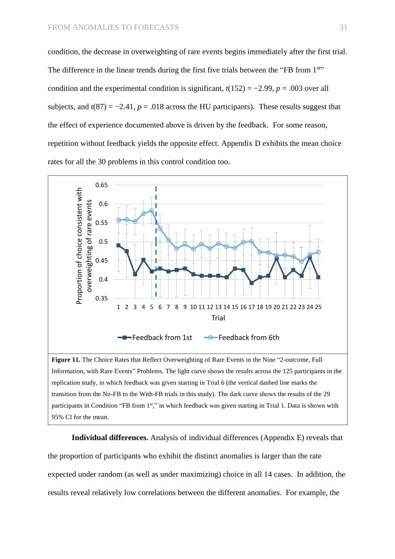
FROM ANOMALIES TO FORECASTS 31
condition, the decrease in overweighting of rare events begins immediately after the first trial.
The difference in the linear trends during the first five trials between the “FB from 1st”
condition and the experimental condition is significant, t(152) = −2.99, p = .003 over all
subjects, and t(87) = −2.41, p = .018 across the HU participants). These results suggest that
the effect of experience documented above is driven by the feedback. For some reason,
repetition without feedback yields the opposite effect. Appendix D exhibits the mean choice
rates for all the 30 problems in this control condition too.
Figure 11. The Choice Rates that Reflect Overweighting of Rare Events in the Nine “2-outcome, Full
Information, with Rare Events” Problems. The light curve shows the results across the 125 participants in the
replication study, in which feedback was given starting in Trial 6 (the vertical dashed line marks the
transition from the No-FB to the With-FB trials in this study). The dark curve shows the results of the 29
participants in Condition “FB from 1st,” in which feedback was given starting in Trial 1. Data is shown with
95% CI for the mean.
Individual differences. Analysis of individual differences (Appendix E) reveals that
the proportion of participants who exhibit the distinct anomalies is larger than the rate
expected under random (as well as under maximizing) choice in all 14 cases. In addition, the
results reveal relatively low correlations between the different anomalies. For example, the
0.35
0.4
0.45
0.5
0.55
0.6
0.65
1 2 3 4 5 6 7 8 9 10 11 12 13 14 15 16 17 18 19 20 21 22 23 24 25
Pro
po
rtio
n o
f ch
oic
e co
nsi
sten
t w
ith
o
verw
eigh
tin
g o
f ra
re e
ven
ts
Trial
Feedback from 1st Feedback from 6th

FROM ANOMALIES TO FORECASTS 32
correlation between overweighting of rare events and the Allais pattern is 0.0008, and the
correlation between loss aversion and risk aversion in the St. Petersburg problem is only 0.07
(p = 0.46). Most of the large correlations could be the product of a “same choices bias” (the
same choice rates are used to estimate two anomalies). The largest correlation free of the
same choice bias involves the negative correlation (r = −0.39) between overweighting of rare
events and risk aversion in the St. Petersburg problem, suggesting that the attitude toward
positive rare events reflects a relative stable individual characteristic.
Effects of location and order. Recall that the experimental condition was run in two
locations, the Technion and HU, under two orders (as explained in Footnote 2). Differences
were found to be minor. The correlations between HU and the Technion and between the two
orders were 0.92 or higher. Moreover, for the purposes of the current study, any existing
differences were of little interest, as all the behavioral phenomena from Table 1 were
reproduced in both locations and most emerged in both locations and order conditions.7
Calibration: Randomly Selected Problems
As noted above, the replication study focuses on 30 carefully selected points in an
11-dimensional space of choice tasks. The results demonstrate that our space is wide enough
to replicate the classical choice anomalies. However, our analysis also highlights the fact that
the classical problems are a small non-random sample from a huge space. Thus, the attempt
7 Some behavioral phenomena, such as the splitting effect and loss aversion, were more common under
the ByFB condition, and other phenomena, such as the break-even effect and the reversed reflection effect, were
more common under the ByProb condition. The largest effect of the order was observed in Trial 6. The ByProb
subjects faced this trial immediately after Trial 5, and exhibited similar behavior to their behavior in that trial.
The ByFB subjects faced many other tasks between Trial 5 and Trial 6 (they first completed the No-FB block in
all problems, and typically also played some problems, 15 on average, with feedback). This gap was associated
with less overweighting of rare events by the ByFB group in Trial 6. Yet, in general, the qualitative differences
are minor.

FROM ANOMALIES TO FORECASTS 33
to develop a model based on the results of the replication study can lead to over-fitting the
classical anomalies. The current study is designed to reduce this risk of over-fitting by
studying 60 new problems selected randomly from the space of problems described above.
Since the two framing manipulations did not reveal interesting effects in the replication study,
the current study focuses only on the abstract representation. Appendix F shows the problem-
selection algorithm. This algorithm implies an inverse relationship between risks and rewards
(correlation of −0.6), a characteristic of many natural environments (Pleskac & Hertwig,
2014). Appendix G details the 60 problems selected.
Method
One hundred and sixty-one students (81 male, MAge = 25.6) participated in the
calibration study.8 Each participant faced one set of 30 problems from Appendix G: 81
participants faced Problems 31 through 60 and the rest faced Problems 61 through 90. The
experiment was run both at the Technion (n = 81) and at HU. The apparatus and design were
similar to those of the replication study. In particular, participants faced each problem for 25
trials, the first five trials without feedback (no-FB), and the rest with full (including the
forgone outcome) feedback (with-FB). Participants were paid for one randomly selected trial
in one randomly selected problem in addition to a show-up fee (determined as in the
replication study). The final payoff ranged between 10 and 144 shekels (M = 47.7).
8 Due to an experimenter error at the Technion, several participants of the current study also
participated in the replication study and a few participated in the current study twice. Because this error was
only revealed late into the competition, the published data includes these participants. However, we ran
robustness checks to make sure that the results are unaffected by these participants: We compared the published
mean choice rates with the rates that would be obtained had we excluded their second participation and found
virtually no differences between the two.

FROM ANOMALIES TO FORECASTS 34
Results and Discussion
The mean choice rates per block and by feedback type (i.e., no-FB or with-FB) for
each of the 60 problems are summarized in Appendix G. The raw data is provided in the
online supplemental material (http:\\departments.agri.huji.ac.il/cpc2015). Below we
summarize the main results.
Full information problems. Analysis of the 46 full information (non-ambiguous)
problems (i.e., those that do not involve ambiguity, Amb = 0) in which the two options had
different expected values (EV) shows a preference for the option with the higher EV. The
maximization rate (i.e., choice rate of the higher-EV option) in the no-FB trials was 64%
(SD = 0.18). In 26 problems, this maximization rate differed significantly from 50% (at .05
significance level, corrected for multiple comparisons according to the procedure by
Hochberg, 1988), and in 24 of these, this rate was higher than 50%. In only two problems
(Problem 44 and Problem 61, see Figure 12) the maximization rate in the no-FB trials was
significantly lower than 50%. The initial deviation from maximization in both problems may
reflect overweighting of rare events. Figure 12 shows that feedback reduced these deviations,
but did not reverse them.

FROM ANOMALIES TO FORECASTS 35
Prob. Option A Option B
44 (23, 1)
[EV=23]
(−33, .01; 24)
[EV= 23.43]
61 (25, .75; 26)
[EV= 25.25]
(23, .025; 24, .95; 25, .0125;
29, .00625; 37, .00313;
53, .00156; 85, .00078;
149, .00078)
[EV= 24.25]
Figure 12. Problems with Initial Low Maximization Rates in the Calibration Study. The notation (x1, p1;
x2, p2; …; y) refers to a prospect that yields a payoff of x1 with probability p1, a payoff of x2 with probability
p2, …, and y otherwise. Maximization rates are shown in five blocks of five trials each (Block 1: “no-FB,”
Blocks 2–5: “with-FB”), and are given with 95% CI for the mean.
Feedback increased maximization. Total maximization rate in the with-FB trials was
67% (SD = 0.21). In 10 of the 11 problems in which choice rates in the no-FB and with-FB
trials significantly differed; maximization rates were higher in the with-FB trials. Analysis of
these ten problems reveals they have a property in common. In all ten problems, the option
that maximizes expected value also minimized probability of immediate regret by providing
the higher payoff most of the time (see Erev & Roth, 2014). Congruently, in the only problem
in which feedback significantly decreased maximization rates (Problem 39, see Figure 14),
the maximizing option provided a better payoff in only 20% of the trials. Figure 13 confirms
the generality of this finding. It examines all 46 relevant problems and shows that the higher
the proportion of better payoffs generated by the maximizing option (i.e. the lower the
probability of regretting a maximizing choice), the larger the increase in maximization rates
brought about by feedback (and vice versa). The correlation between the two is 0.65, 95% CI
[0.45, 0.79]. In other words, the addition of feedback increased the choice rate of the prospect
that minimizes the probability of the regret a decision maker experiences after observing he
0.00
0.25
0.50
0.75
1.00
1 2 3 4 5
P(M
ax)
Block
44: 23 with certainty
61: (25, .75; 26)
0.00
0.25
0.50
0.75
1.00
1 2 3 4 5
P(M
ax)
Block
44: 23 with certainty
61: (25, .75; 26)

FROM ANOMALIES TO FORECASTS 36
or she selected the option that generated the lower payoff in a particular trial (see related
ideas in Hart, 2005; Loomes & Sugden, 1982; Sarver, 2008).
Figure 13. Increase in Choice of the Maximizing Option between With-FB and No-FB trials as a Function of
the Probability that the Maximizing Option Provides Higher Payoff than the Low EV Option in a Random
Trial in the Calibration Study. Each data point represents one problem and is marked with the number of that
problem (see Appendix G). The bold dark markers represent problems with maximization increase
significantly different from zero. The correlation is .65.
Figure 14 demonstrates this observation in four problems: two problems (36 and 70)
in which feedback moved participants towards maximization and two problems (39 and 52)
in which it moved participants away from maximization. The effect of experience in all four
problems is consistent with the hypothesis that feedback increases the tendency to select the
option that is better most of the time and minimizes the probability of immediate regret. Note,
in addition, that the initial maximization rates in three of these problems are in the direction
predicted by several phenomena given in Table 1 (loss aversion in Problems 36, 52, and 70;
break-even effect in Problem 52; and the certainty effect in Problems 36 and 70).
32
33
34
37
3840
41
46
47
51
52
53
54
5556
57
58
59
60
61
6263
65
66
67
6871
73
75
77 78
80 84
85
90
-0.25
-0.2
-0.15
-0.1
-0.05
0
0.05
0.1
0.15
0.2
0.25
0 0.2 0.4 0.6 0.8 1
Maxim
iza
tio
n I
ncre
ase
P(Max Option Better)

FROM ANOMALIES TO FORECASTS 37
Prob. Option A Option B P(Max. Better)
36 (28, 1)
[EV= 28]
(−46, .4; 86, .3;
88, .15; 92, .15)
[EV= 34.4]
60%
39 (29, 1)
[EV= 29]
(6, .2; 31, .05; 32, .2;
33, .3; 34, .2; 35, .05)
[EV= 27.6]
20%
52
(46, .2; 0)
[EV= 9.2]
(46, .25; −2)
[EV= 10]
25%
(20% + 5% tie)
70
(18, 1)
[EV= 18]
(35, .75; −19)
[EV= 21.5]
75%
Figure 14. Problems that Demonstrate the Typical Effect of Feedback in the Calibration Study. The notation
(x1, p1; x2, p2; …; y) refers to a prospect that yields a payoff of x1 with probability p1, a payoff of x2 with
probability p2, …, and y otherwise. P(Max. Better) is the probability that the maximizing option provides
better payoff than the low EV option in a random trial. Maximization rates are shown in five blocks of five
trials each (Block 1: “no-FB,” Blocks 2–5: “with-FB”) and are given with 95% CI for the mean.
Figure 15 summarizes the results for the three full information problems that include
two options with identical EVs. All three problems involve choice between a safe gain and a
multi-alternative symmetric-distribution gamble with the same expected value. The observed
choice rates in the no-FB trials (Block 1) suggest risk neutrality; the gamble’s choice rates
were 50%, 54%, and 44% for problems 45, 49, and 50 respectively (SD = 0.45, 0.46, and
0.44). In none of the problems is the difference from 50% statistically significant:
t(80) = −0.07, 0.75, and −1.3 respectively. Moreover, in two of the three problems, feedback
increased risk taking. These results differ from the common observation of risk aversion in
the gain domain (e.g., Kahneman & Tversky, 1979) and are consistent with recent studies that
demonstrated that feedback can lead to risk seeking in the gain domain (Ludvig & Spetch,
2011; Tsetsos, Chater, & Usher, 2012). The initial risk neutrality could be the product of the
multi-outcome symmetric distribution used here. Another feasible explanation involves the
0.00
0.25
0.50
0.75
1.00
1 2 3 4 5
P(M
ax)
Block
36: 60% max. better
70: 75% max. better
0.00
0.25
0.50
0.75
1.00
1 2 3 4 5
P(M
ax)
Block
39: 20% max. better
52: 25% max. better

FROM ANOMALIES TO FORECASTS 38
fact that in Problems 45 and 49 (where we observe the higher risk-seeking rates) the worst
possible outcome from the gamble is high relative to the safe alternative.
Prob. Option A Option B
45 (13, 1) (9, .00391; 10, .03125;
11, .10938; 12, .21875;
13, .27344; 14, .21875;
15, .10938; 16, .03125;
17, .00391)
49 (23,1) (22, .25; 23, .5; 24, .25)
50 (4, 1) (0, .00391; 1, .03125;
2, .10938; 3, .21875;
4, .27344; 5, .21875;
6, .10938; 7, .03125;
8, .00391)
Figure 15. Problems with Identical Expected Values in the Calibration Study. The notation (x1, p1;
x2, p2; …; y) refers to a prospect that yields a payoff of x1 with probability p1, a payoff of x2 with probability
p2, …, and y otherwise. Proportions of the riskier choice are shown in five blocks of five trials each (Block 1:
“no-FB,” Blocks 2–5: “with-FB”), and are given with 95% CI for the mean.
Another contribution of the full information calibration problems is the suggestion
that the loss aversion bias may be less robust to feedback than suggested by Problems 12, 13,
and 14 (Figure 4) of the replication study. For example, in Problem 75 (“13 with certainty”
or “50, .6; −45”), experience increased the choice rate of the counterproductive mixed gamble
(EV of 12) from 35% to 50%.
Ambiguous problems. Results of the 11 ambiguous problems replicate the main
findings from the replication study. Specifically, the results show that the initial behavior (no-
FB trials) reflects some pessimism and a tendency to maximize expected return assuming all
outcomes of the ambiguous option are equally likely. Feedback tends to increase
maximization; the choice rates of the ambiguous option tend to decrease when the ambiguous
option is objectively inferior to the alternative and increase when the opposite is true.
0.00
0.25
0.50
0.75
1.00
1 2 3 4 5P
(B)
Block
45: EV = 13
49: EV = 23
50: EV = 4

FROM ANOMALIES TO FORECASTS 39
Capturing the Joint Effect of the 14 Behavioral Phenomena
The main goal of this section is to propose a model that can capture the joint effect of
the 14 phenomena discussed above and the interactions between them. Specifically, the
competition’s organizers (EEP) attempted to develop a simple model that could reproduce the
initial choice rates and the effects of feedback in all 90 problems from the replication and
calibration studies, and serve as a baseline model for a choice prediction competition.
The relatively high maximization rates led EEP to assume the model should include
high sensitivity to the expected value (EV) rule and focus their model development on the
deviations from the prescription of this rule. This analysis shows that nearly all of the
anomalies can be described as the product of (at least one of) the following four tendencies:
(a) Equal weighting, a tendency toward the option expected to lead to the best payoff
assuming that all the outcomes are equality likely. This tendency captures the Allais paradox,
overweighting of rare events, and the splitting effect. (b) Payoff sign, a tendency toward the
option that maximizes the probability of the best possible payoff sign. This tendency captures
the reflection effect, the break-even effect, and the get-something effect. (c) Pessimism, a
tendency to assume the worst. This tendency explains the Allais paradox, loss aversion, risk
aversion in the St. Petersburg problem, and the Ellsberg paradox. (d) Minimization of regret,
a tendency to select the option that minimizes the probability of immediate regret. This
tendency captures the experience phenomena: underweighting of rare events, reversed
reflection, the payoff variability effect, and the correlation effect. The results also suggest that
the tendency to favor the option that minimizes the probability of regret increases with
feedback.
Integrating Expected Value and the Four Tendencies
The observation that the main experimental results can be captured with the assertion
that decision makers (a) are highly sensitive to the expected value and (b) exhibit four

FROM ANOMALIES TO FORECASTS 40
behavioral tendencies, naturally raises the question of how these elements should best be
integrated into one model. In answering this question, EEP made three main modelling
decisions.
The first decision involves the basic question of how the four tendencies should be
implemented. The most popular approach for capturing behavioral tendencies of this sort
assumes they are reflections of hard-wired subjective functions of values and/or probabilities.
Expected utility theory and prospect theory are two prominent examples of this approach. For
instance, prospect theory captures the tendency to prefer the status quo over a mixed gambles
with the same EV (see problem 12) by assuming asymmetric subjective value function,
whereas a tendency to overweight rare events and underweight medium-probability events is
captured by assuming an S-shape weighting function. As discussed in preceding text,
however, the main shortcoming of this popular approach is that it is difficult to find functions
that capture all the anomalies addressed here with one set of assumptions and parameters.
This shortcoming led EEP to follow an alternative approach for implementing the four
tendencies. They assumed that the distinct tendencies reflect the use of specific cognitive
strategies, or “tools,” which may be particularly useful in certain settings (Gigerenzer, Todd,
& ABC Group, 1999). For example, a tendency to behave pessimistically can be useful when
decision makers face adversarial settings. Yet, the use of the tool in settings in which it is
inappropriate leads to the behavioral anomalies.
A second modelling decision EEP made involves the output of the decision tools.
Assuming that the tools are used to simplify the decision making process, it is natural to use
their output to determine the final choice (i.e., prescribe choice of Option A, choice of Option
B, or indifference; as in Dhami, 2003; Ert, Erev, & Roth, 2011; Gigerenzer et al., 1999;
Payne, Bettman, & Johnson, 1993) Under an alternative abstraction, the output of the tools is
“just another estimate” of the expected benefit from a specific choice, and this estimate is

FROM ANOMALIES TO FORECASTS 41
weighted with other estimates. EEP chose the just-an-estimate abstraction. Their choice
reflects the observation that the results reveal sensitivity to the magnitude (and not only the
direction) of the differences in expected values. For example, consider Problem 11 (“19 with
certainty” or “20, .9; −20”, EV = 16) and Problem 75 (“13 with certainty” or “50, .6; −45”,
EV = 12). Both problems are similar in the sense that the tendency to minimize the
probability of regret favors the gamble and contradicts the prescription of the EV rule (and
the other three tendencies agree with the EV rule). The results show stronger deviations from
maximization in Problem 75 (50% in the last block), than in Problem 11 (21% in the last
block). This difference suggests that the impact of the tendency to minimize probability of
regret decreases with the expected cost of this behavior.
The final modelling decision EEP made involves the question of whether the values
the tools generate are deterministic or depend on the option’s payoff variability. Analysis of
the current data shows that the latter possibility is the more reasonable one. For example,
compare Problem 23 (“2 with certainty” or “3 with certainty”) with Problem 54 (“18 with
certainty” or “64, .5; −33”, EV = 15.5). All four tendencies agree with the EV rule in both
problems. Yet, the results show a large difference: high maximization rates in problem 23
(97% without and 99% with feedback), and much lower rates in Problem 54 (68% without
and 70% with feedback). Thus, the results suggest more choice variability in the problem
with higher payoff variability (see a similar observation by Busemeyer, 1985). To address
this and similar observations, EEP abstracted the processes that underlie the four tendencies
as “sampling tools” (rather than deterministic tools, which are similar to simple heuristics).
Specifically, the use of a “sampling tool” implies that the decision maker mentally samples
outcomes from payoff distributions that correspond to the underlying tendency. This
abstraction is explained in more detail in the next section, which describes the baseline
model.

FROM ANOMALIES TO FORECASTS 42
Clearly, making the above three modelling decisions does not define a unique model.
There are many possible abstractions that assume high sensitivity to the expected value in
addition to four tendencies implemented as the product of sampling tools. We now turn to
present the best such model EEP were able to find dubbed “Best Estimate And Sampling
Tools” (BEAST).
Baseline Model: Best Estimate And Sampling Tools (BEAST)
BEAST assumes that the attractiveness of each prospect is the sum of the best
estimate of its EV (estimated pessimistically in ambiguous gambles) and the mean value
generated by the use of sampling tools that correspond to the four behavioral tendencies.
Quantitatively, BEAST assumes that Option A is strictly preferred over Option B, after r
trials, if and only if:
[BEVA(r) − BEVB(r)] + [STA(r) – STB(r)] + e(r) > 0 (1)
where BEVA(r) – BEVB(r) is the advantage of A over B based on the best estimation of their
expected values, STA(r) – STB(r) is the advantage of A over B based on the use of sampling
tools, and e(r) is an error term.9 In trivial choices, when one of the options dominates the
other, e(r) = 0.10 In all other cases, e(r) is drawn from a normal distribution with a mean of 0
and standard deviation of σi (a property of agent i).
When the payoff distributions are known (as in the non-ambiguous problems in our
study), the best estimations of the expected values are the actual objective ones. That is,
BEVj(r) equals the expected value of option j, EVj (for all r). The value of option j based on
9 When the left-hand side of Inequality (1) equals exactly zero, we assume random choice between the
options.
10 In dominance, we mean either deterministic dominance or first-order stochastic dominance. In the first
90 problems (i.e., the replication and calibration studies), the trivial problems are problems 28, 29, 30, 38, 43, 72,
74, 81, 83, 84, and 89.

FROM ANOMALIES TO FORECASTS 43
the use of the sampling tools, STj(r), equals the average of κi (a property of i) outcomes that
are each generated by using one sampling tool.11
There are four possible sampling tools. Sampling tool unbiased was introduced to
capture the tendency to minimize immediate regret that implies a preference for the option
that produces a higher outcome most of the time (in one random trial, rather than on average).
It can be described as random and unbiased mental draws, either from the options’ described
distributions or from the options’ observed history of outcomes. Before obtaining feedback
(decisions in Trials 1 to 6), the draws are taken from the objective distributions using a luck-
level procedure. First, the agent draws a luck-level, a uniform number between zero and one.
Then, for each prospect, the agent uses the same luck-level as a percentile in the prospect’s
cumulative distribution function and draws the outcome that fits that percentile.12 When the
agents can rely on feedback (Trials 7 to 25), they first sample one of the previous trials (all
with-FB trials are equally likely to be sampled), and the drawn outcomes for both options are
those observed in that trial.
The other three sampling tools are “biased.” They can be described as a mental draw
from distributions that differ from the objective distributions. The probability of choosing one
of the biased tools, PBias, decreases when the agent receives feedback. Specifically,
PBias(t) = βi / (βi + 1+ tθi), where βi > 0 captures the magnitude of the agent's initial tendency
to use one of the biased tools, t is the number of trials with feedback, and θi > 0 captures
11 For example, consider an agent with κi = 3 who faces Problem 17 (“30” or “50, .5; -1”) based on the
following sampling tools results {30, 50}, {30, 50}, and {30, -1} and the error term e(r) = -2. The left-hand side
of Inequality (1) yields (30 − 24.5) + (90/3 − 99/3) − 2 = 0.5. Thus, the model implies an A choice.
12 That is, the outcome drawn is the result of F-1(x), where x is the luck-level and F-1 is the prospect’s
inverse cumulative distribution function. For example, in Problem 2 (“3, .25; 0” or “4, .2; 0”), a luck level of .67
yields the draw {0, 0}, a luck level of .77 yields the draw {3, 0}, and a luck level of .87 yields the draw {3, 4}.

FROM ANOMALIES TO FORECASTS 44
agent i's sensitivity to feedback.13 The assumption that the probability of using the unbiased
tool increases with feedback was introduced to capture the observation that the main
deviations from maximization after obtaining feedback—the four “experience” phenomena in
Table 1—suggest increased sensitivity to the probability of regret.
The three biased tools are each used with equal probability, PBias(t)/3. The sampling
tool uniform yields each of the possible outcomes with equal probability (see a related idea
by Birnbaum, 2008) using the luck-level procedure described above (the draws are made
from the uniform cumulative distribution function even after feedback is obtained). This tool
corresponds to the tendency “equal weighting” and therefore helps the model capture the
Allais paradox, overweighting of rare events, and the splitting effect.
The sampling tool contingent pessimism is similar to the priority heuristic
(Brandstätter et al., 2006); it depends on the sign of the best possible payoff (SignMax) and
the ratio of the minimum payoffs (RatioMin). When SignMax > 0 and RatioMin ≤ γi
(0 < γi < 1 is a property of i), this tool yields the worst possible payoffs for each option (MINA
and MINB). It corresponds to the tendency to be pessimistic, and helps the model capture loss
aversion, the certainty effect, and risk aversion in the St. Petersburg paradox. When one of
the two conditions is not met, the current tool implies random choice among the possible
payoffs (identically to the uniform tool). RatioMin is computed as:
A B
A B
A B A B
A B
1, if
Min ,, if and sign( ) sign( )
Max ,
0, otherwise
MIN MIN
MIN MINRatioMin MIN MIN MIN MIN
MIN MIN
(2)
13 For example, assuming βi = 3, and θi =.5, the probability of using one of the biased tools in each of
the κi simulations is 3/(3+1) =.75 when t = 0 (Trials 1 to 6), 3/(3+1+1) = .6 when t = 1 (Trial 7), and
3/(3+1+3.36) = .407 when t = 19 (Trial 25).

FROM ANOMALIES TO FORECASTS 45
For example, RatioMin = 0 in Problem 9 (“1” or “100, .01; 0”), and 0.5 in Problem 10 (“2” or
“101, .01; 1”). The contingencies capture two regularities. The sensitivity to SignMax implies
less pessimism (less risk aversion) in the loss domain, hence the reflection effect. The second,
RatioMin contingency, implies less pessimism when the minimal outcomes appear similar
(have the same sign and are close in magnitude). This implies that the addition of a constant
to all the payoffs decreases risk aversion in the gain domain. In addition, it implies higher
sensitivity to rare events in problems like Problem 10 and Problem 61 (large RatioMin) than
in problems like Problem 9 and Problem 25 (small RatioMin).
The sampling tool sign implies high sensitivity to the payoff sign (Payne, 2005). It is
identical to the tool unbiased, with one important exception: positive drawn values are
replaced by R, and negative outcomes are replaced by −R, where R is the payoff range (the
difference between the best and worst possible payoffs in the current problem; e.g., 100 in
Problem 9 and Problem 10).14 It enables the model to capture the reflection effect, the break-
even effect and the get-something effect.
When the probabilities of the different outcomes are unknown (as in the problems
with ambiguous Option B), they are initially estimated with a pessimistic bias (Gilboa &
Schmeidler, 1989). The initial expected value of the ambiguous option is estimated as a
weighted average of three terms: EVA, MINB, and UEVB, the latter being the estimated EV
from Option B, under the assumption that all the possible outcomes are equally likely. The
model assumes the same weighting for EVA and UEVB and captures the weighting of MINB
with 0 ≤ φi ≤ 1, an ambiguity aversion trait of agent i. That is,
BEVB(0) = (1 − φi)(UEVB + EVA)/2 + φi∙MINB, (3)
14 For example, in Problem 9 (“1” or “100, .01; 0”), all the positive outcomes are replaced by +100 (the
value of R), and the 0 remains 0.

FROM ANOMALIES TO FORECASTS 46
For example, assuming φi = 0.05, BEVB(0) in Problem 22 (“10, .1; 0” or “10, p; 0”) equals
.95(5+1)/2 + .05(0) = 2.85. In decisions made prior to receiving feedback (Trials 1 to 6) the
probabilities of the m possible outcomes are estimated under the assumption that the
subjective probability of the worst outcome, SPMINB, is higher than 1/m, and each of the other
m − 1 subjective probabilities equals (1 − SPMINB)/(m − 1). Specifically, SPMINB is computed
as the value that minimizes the difference between BEVB(0) and the estimated expected value
from Option B based on the subjective probabilities: SPMINB∙MINB + (1 − SPMINB)∙UBh, where
UBh = (m∙UEVB − MINB)/(m − 1) denotes the average of the best m − 1 outcomes. This
assumption implies that
B
B B
B
B
0, if 0 >
1, if 0 <
0,otherwise
Bh
MINB
Bh
Bh
BEV U
SP BEV MIN
U BEV
U MIN
(4)
That is, in Problem 22 with φi = 0.05, SPMINB = (10 − 2.85)/(10 − 0) = 0.715.
Each trial with feedback in the ambiguous problems moves BEVB(t) toward EVB.
Specifically,
BEVB(t + 1) = (1 − 1/T)∙BEVB(t) + (1/T)∙OB(r) (5)
where T is the expected number of trials with feedback (20 in the current setting) and OB(r) is
the observed payoff generated from the ambiguous Option B at trial r.15
The six properties of each agent are assumed to be drawn from uniform distributions
between 0 and the model's parameters: σi ~ U(0, σ), κi ~ (1,2, 3, ..., κ), βi ~ U(0, β),
θi ~ U(0, θ), γi ~ U(0, γ), and φi ~ U(0, φ). That is, the model has six free parameters: σ, κ, β,
γ, φ, and θ. Note that only four of these parameters (σ, κ, β, and γ) are needed to capture
15 For example, in Problem 22 with φi = 0.05, observing OB(6) = 0 implies that
BEVB(1) = (1 − 1/20)∙2.85 + (1/20)∙0 = 2.707.

FROM ANOMALIES TO FORECASTS 47
decisions under risk without feedback (the class of problems addressed by prospect theory).
The parameter φ captures attitude toward ambiguity, and θ abstracts the reaction to feedback.
BEAST’s parameters were estimated using the mean squared deviation (MSD)
measure and 14 additional constraints that correspond to the 14 qualitative phenomena
summarized in Table 1. Specifically, we used a grid search procedure to find the set of
parameters that minimizes the MSD over the 450 B-rates (90 problems times 5 blocks) and
also reproduces the 14 qualitative phenomena. Best fit was obtained with the parameters
σ = 7, κ = 3, β = 2.6, γ = .5, φ = .07, and θ = 1. The MSD score is 0.0073. The right-hand
graphs in Figures 1 through 10 present the predictions of BEAST with these parameters.
BEAST, individual differences, and inertia. Notice that under BEAST, each choice
is affected by at least 6 + κi independent draws from the uniform distribution [0, 1], and one
draw from a normal distribution. The first six draws determine the agent's properties (the
values σi, κi, βi , θi, γi, φi), κi uniform draws determine the sampling tools used (and, in most
cases, the outcomes these tools imply are determined by additional independent uniform
draws, e.g., for the luck levels), and the normal draw is the error term. The timing of these
draws does not affect the model's aggregate predictions, but it does affect the predicted
individual differences and inertia statistics. The basic version of BEAST assumes that the six
properties are drawn before the experiment starts (when the virtual agent is “born”), and the
other draws are taken before each choice. Appendix E shows that with this assumption the
model under-predicts the magnitude of the correlations among the different phenomena.
Additional analysis shows that the basic version of BEAST also under-predicts the inertia
level (the tendency to repeat the last choice). The observed inertia level is 0.87 before
feedback and 0.83 with feedback, and BEAST predictions are below 0.65.
These results remind us that BEAST can be improved, and also suggest a natural way
to improve it. Stronger individual differences and higher inertia rates can easily be captured

FROM ANOMALIES TO FORECASTS 48
by changing the assumptions concerning the timing of the random draws (e.g., the sampling
tools used or luck levels) that underlie the predictions of BEAST. Since changes of this type
cannot affect the aggregate predictions of BEAST, which are the focus of the current paper,
we chose to leave the refinement of the abstraction of the individual difference statistics to
future research.
A Choice Prediction Competition
The experimental results summarized above suggest that the main deviations from
maximization presented in Table 1 can be reliably observed in our 11-dimensional space of
problems. In addition, the above analysis suggests that the coexistence of distinct deviations
in contradicting directions (e.g., over- and under-weighting of rare events) can be captured
with a single quantitative model that assumes sensitivity to the expected return and four
additional behavioral tendencies (the product of using sampling tools), one of which, regret
minimization, becomes more prominent when decision makers can use feedback.
The main shortcoming of this analysis is the fact that BEAST, the quantitative model
EEP proposed, lives up to its name: it is not elegant in the sense that the exact
implementation of the different sampling tools includes some post-hoc assumptions that were
introduced to capture the current results. Thus, it is possible that it over-fits the data, and
better models exist or can be easily developed. Moreover, in developing BEAST, EEP made
three major modelling decisions that narrowed the space of possible models they considered,
potentially ignoring better descriptive models. In particular, the fact that EEP did not find it
easy to develop a useful and elegant model using “subjective functions” of values and
probabilities (like prospect theory, and most other decision making models) does not mean
that it is impossible to find one. To explore these possibilities, EEP organized a choice
prediction competition (see Arifovic et al., 2006; Erev, Ert, Roth, et al., 2010; Erev, Ert, &

FROM ANOMALIES TO FORECASTS 49
Roth, 2010; Ert et al., 2011; and a recent review of this approach in Spiliopoulos & Ortmann,
2014) using a generalization criterion (Busemeyer & Wang, 2000). Specifically, EEP ran a
third, test study, using the design of the calibration study, and challenged other researchers to
participate in an open competition that focuses on the prediction of the results of this
experiment. It should be noted that the use of a generalization criterion (which is similar to
cross validation, except that the validation is tested on new experimental designs) for model
comparisons greatly reduces the risk of choosing an overly complex model because it “puts
the models on equal footing in the generalization stage, despite the fact that the more
complex model has an unfair advantage in the calibration stage” (Busemeyer & Wang, 2000,
p. 179).
The participants of the prediction competition were asked to send the organizers a
model implemented in a computer program that reads the 10 parameters of each problem as
input and provides the predicted mean B-rates in five blocks of five trials as output. The
choice problems of the test set were only revealed, together with the main results, a day after
the submission deadline. Yet, it was common knowledge that the problems would be sampled
from the same space of problems studied in the replication and calibration studies, and that
subjects would be drawn from the same student population (Technion and HU). The potential
competition participants knew that the winning model would be the one with the lowest mean
squared deviation score over the five blocks of trials in the test set. Additionally, to facilitate
accumulation of knowledge, the submitted models had to replicate the 14 phenomena from
Table 1. Moreover, to facilitate the models’ usability for future research they had to be
accompanied by a clear, concise verbal description. This latter requirement signifies a
distinction between our competition (and most competitions organized in the social sciences)
and most tournaments or prediction markets aimed at practical applications (primarily of
interest in computer science), which are not interested in interpretability of the successful

FROM ANOMALIES TO FORECASTS 50
models (Spiliopoulos & Ortmann, 2014). The winning participants (Cohen & Cohen) were
invited to co-author the current paper. Appendix H presents the call for the competition and
its detailed requirements.
Competition Criterion: Mean Squared Deviation (MSD)
The current competition focused on the prediction of the mean B-rates in each of five
blocks of trials for each choice problem. As in previous competitions (Erev, Ert, Roth, et al.,
2010; Erev, Ert, & Roth, 2010; Ert et al., 2011), the accuracy of the predictions was evaluated
using MSD scores. We first computed the squared difference between the observed and
predicted rates in each block of five trials for each of the 60 problems, and then computed the
mean across the 300 scores.
The MSD criterion has several advantages over other model estimation criteria (e.g.,
likelihood criteria). In particular, the MSD score underlies traditional statistical methods (like
regression and the t-test), is a proper scoring rule (Brier, 1950; Selten, 1998), and can be
translated to the intuitive Equivalent Number of Observation (ENO) score explained below.
Note that the use of a proper scoring rule is particularly important in prediction competitions
such as ours, and serves to incentivize participants to nominate “truthful” models rather than
biased ones, from which it is more difficult to derive theoretical insights.
Relationship to Previous Competitions
The current competition addresses the critique of previous choice prediction
competitions (Spiliopoulos & Ortmann, 2014), which asserted that since competitions are
typically run as single implementations, they might be susceptible to auxiliary assumptions.
Therefore “before running a tournament it is important to very carefully select the
implementation details based on prior studies and knowledge” (Spiliopoulos & Ortmann,
2014, p. 243). The starting point of the current competition, which focused on the replication

FROM ANOMALIES TO FORECASTS 51
of 14 well-known behavioral phenomena, follows this proposition. Furthermore, we believe
that the requirement that submitted models be clear in their description so other researchers
can easily use them should facilitate the models’ parsimony and usability.
Another relationship to previous competitions involves the similarity of BEAST to the
model that won the learning-in-games competition (Erev, Ert, & Roth, 2010). This model
(Chen, Liu, Chen, & Lee, 2011) assumes high sensitivity to the estimated expected value
(average payoff), some initial biased tendencies, and reliance on small samples of past
experiences that implies immediate regret minimization. The main difference between
BEAST and the 2010 competition winner is the nature of the initial biased tendencies. Hence,
these tendencies appear to be situation-specific.
Competition Submissions
Fifty-three teams of researchers registered for the competition. Twenty-five of these
teams, with members from five continents, submitted models. The submissions can be
classified into three main categories. The first class, which contains three submissions, builds
primarily on the traditional research approach assuming behavior can be well described by
subjective functions of values and probabilities. Specifically, the typical model in this class
uses a variant of prospect theory that assumes that the parameters of the underlying subjective
functions are situation-specific.
The second class, which consists of 14 submissions, includes models that can be
described as variants of BEAST. In particular, all these models assume high sensitivity to the
expected value and four behavioral tendencies that can be captured by assuming the use of
four sampling tools. Moreover, all but one of these models also share with BEAST the three
modelling decisions EEP made and are discussed above.
The third class, which includes seven submissions, involves models that do not
attempt to directly identify the underlying processes, but rather use machine learning or

FROM ANOMALIES TO FORECASTS 52
similar statistical approaches. Three of the models in this class rely on theoretical insights
taken from the decision making literature as input (explanatory variables, or “features”) for
the models. The four other models in this class can be considered theory-free in the sense that
the features used in these models include primarily the structure of the task (the dimensions
that define it), in the hope that the model can predict the choice rates based on these basic
features.
One submission does not fit in any of these three categories. It is a variant of instance-
based learning (IBL; Gonzalez, Lerch, & Lebiere, 2003) that uses the described payoff
distributions to create mental instances prior to obtaining feedback and then applies an IBL
model as usual.
The Test Set
As noted above, the test set includes 60 problems selected randomly from the space
we study, using the algorithm described in Appendix F. As implied by the wide space of
problems and the random drawing mechanism, the test set included different problems than
those examined in the replication and calibration studies. The selected problems are shown in
Appendix I.
Method. One-hundred and sixty (72 male, MAge = 24.5) students from the Technion
(n = 80) and HU participated in the competition study. Half the participants faced problems
91 through 120 and the others faced problems 121 through 150 (see Appendix I). The
apparatus and design were identical to those of the calibration study. The final payoff ranged
between 10 and 149 shekels (M = 38.9).
Results. The main experimental results are summarized in Appendix I. The results
appear to be similar to those of the calibration study. First, where relevant, the maximization
rate of the full information problems was 68% (SD = 0.17) in the no-FB trials and 72%
(SD = 0.19) in the with-FB trials. Second, Figure 16 (cf. Figure 13) shows the robustness of

FROM ANOMALIES TO FORECASTS 53
participants’ tendency to minimize experienced regret by learning to choose the option that is
better most of the time. The correlation between the measures in Figure 16 is 0.71, 95% CI
[0.55, 0.82]. Third, in the only non-ambiguous problem in which both options had identical
EVs (Problem 129), participants seem to exhibit risk neutrality: B-rates are 46% in the no-FB
trials and 51% in the with-FB trials. The difference from 50% is insignificant in every block
of trials. Finally, behavior in the ambiguous problems reflects an initial tendency to assume
uniform probabilities with some ambiguity aversion, and learning toward maximization.
Figure 16. Increase in Choice of the Maximizing Option between With-FB and No-FB trials as a Function of
the Probability that the Maximizing Option Provides Higher Payoff than the Low EV Option in a Random
Trial in the Competition Study. Each data-point represents one problem and is marked with the number of
that problem (see Appendix I). The bold dark markers represent problems with maximization increase
significantly different from zero. The correlation is .71.
Performance of the Baseline Model, BEAST
Figure 17 presents the correlation between the observed B-rates (Y-axis) and the
predictions of the baseline model BEAST (X-axis) in the no-FB and in the with-FB blocks.
Each point presents one of the 60 problems (using the problem numbers, see Appendix I).
The correlations are 0.95 in both the no-FB and with-FB blocks. Correlations in each block
separately are above 0.94 each. The figure also presents the problems in which BEAST
deviates most from the observed rates. Notice that the failure of BEAST in Problem 122
9192 94
96
97
9899
100
101103
105
106107
108
109
113114 115
116
117
118
119
120
122123
125126
128
130
134135
136140
141
143
144
145146149
95
104
110
111
112121
124131
132
133
138
139
142
147
150
-0.25
-0.2
-0.15
-0.1
-0.05
0
0.05
0.1
0.15
0.2
0.25
0 0.2 0.4 0.6 0.8 1
Maxim
ization I
ncre
ase
P(Max Option Better)
9192 94
96
97
9899
100
101103
105
106
107
108
109
113114
115
116
117
118
119
120
122123
125126
128
130
134
135
136140
141
143
144
145146149
95
104
110
111
112121
124131
132
133
138
139
142
147
150
-0.25
-0.2
-0.15
-0.1
-0.05
0
0.05
0.1
0.15
0.2
0.25
0 0.2 0.4 0.6 0.8 1
Maxim
iza
tio
n I
ncre
ase
P(Max Option Better)

FROM ANOMALIES TO FORECASTS 54
implies less overweighting of rare events than predicted by BEAST. We discuss the other
large misses (Problems 93, 126, and 137) below.
B-rate
Problem Option A Option B No-FB With-FB
93 5 with certainty −9, p1; 92, p2; 100, p3; 104, p4; 106, p5
(p1 = .9, p2 = .0125, p3 = .0125, p4 = .025, p5 = .05 unknown)
.56 .39
122 −14, .95; 68, .05 −36, .1; −11, .9 .36 .42
126 −8 with certainty −18, .8; 77, .00313; 78, .0188, 79, .0469; 80, .0625;
81, .0469; 82, .0188; 83, .00313
.53 .51
137 3 with certainty 2, p1; 3, p2; 4, p3; 5, p4; 6, p5
(p1 = .025, p2 = .7, p3 = .15, p4 = .1, p5 = .025 unknown)
.73 .89
Figure 17. BEAST Predictions vs. Observed B-rates by Problem in the Competition Study. Each data point
represents one problem and is marked with the number of that problem (see Appendix I). The diagonal is the
best possible prediction. The red markers represent four problems in which BEAST deviates the most from the
observed choice rates. The table below details these problems and their observed choice rates.
The MSD score of BEAST, across the five blocks and 60 problems, is 0.0098.
Although this value is larger than the corresponding value in Studies 1 and 2 (0.0073),
considering the fact that the parameters were estimated to fit the replication and calibration
studies, the difference is not large. To clarify the implication of the MSD score, we computed
the implied Equivalent Number of Observation (ENO) score (Erev, Roth, Slonim, & Barron,
91
92
94
95
96
97
98
99
100
101
102
103104105
106
107
108
109
110
111
112
113
114
115
116
117
118
119
120
121123
124
125127
128
129
130
131
132
133
134
135
136138
139
140
141
142
143
144145
146
147
148
149
150
93
122
126
137
0
0.1
0.2
0.3
0.4
0.5
0.6
0.7
0.8
0.9
1
0 0.5 1
Observ
ed B
-Rate
BEAST Prediction
No-Feedback block
91
92
94
95
96
97
98
99
100
101
102
103
104105
106
107
108
109
110
111
112
113114
115
116
117
118
119
120
121
123
124
125
127
128129
130
131
132133
134
135
136138
139
140
141
142
143
144145
146
147
148
149
150
93122
126
137
0
0.1
0.2
0.3
0.4
0.5
0.6
0.7
0.8
0.9
1
0 0.5 1O
bserv
ed B
-Rate
BEAST Prediction
With-Feedback Blocks

FROM ANOMALIES TO FORECASTS 55
2007). The ENO of a model is an estimation of the number of subjects that has to be run until
the mean choice rate in each problem provides a better prediction for the behavior of the next
subject than the prediction of the model. The ENO of BEAST in the current setting is 12.07.
That is, the average error of BEAST, over the 60 problems, is smaller than the average error
when predicting the next subject based on the mean choice rates of the first 12 subjects.
The Winning Model and the Performance of Other Submissions.
Twenty-five models were submitted to the competition, and were tested together with
the baseline model, BEAST. Four models failed to replicate at least one of the phenomena in
Table 1 (i.e., failed to comply with the “replication” criterion, detailed in the competition’s
website, as explained in appendix H).16 The other 21 models were ranked according to their
predictions’ MSD on the test set. All 12 top models were variants of the BEAST model.
These models’ MSDs ranged between 0.0089 and 0.0114. Seven of these models had better
MSDs than the baseline BEAST. The other nine models achieved MSDs ranging between
0.0124 and 0.0501.
The winning model, referred to as Cohen’s BEAST (see Appendix J for details) is a
version of BEAST that includes a tendency to avoid “complex prospects” that include
multiple outcomes and/or ambiguity when the payoff range is large, as in Problems 93 and
126. The model also includes a tendency to favor such complex prospects when the payoff
range is narrow, as in Problem 137. Cohen’s BEAST achieved MSD of 0.0089 and ENO of
13.51. It also outperformed all other variants of BEAST in fitting the calibration data (MSD
of 0.0059).
16 Nevertheless, we tested these models on the test set as well. The results revealed that had these
models participated in the competition, they would have been ranked relatively low compared to the other
submissions.

FROM ANOMALIES TO FORECASTS 56
To examine the robustness of the competition’s ranking, we performed a bootstrap
analysis on the submitted models’ scores compared to the competition’s winner. Specifically,
we simulated 1,000 sets of 60 test problems each by randomly sampling from the original test
set (with replacement) and computed the MSD of each submitted model in each simulated
set. Then, we computed the 1,000 differences between each model’s MSDs and the winner’s
MSDs. By removing the 25 smallest MSD differences and the 25 largest MSD differences,
we constructed for each model a 95% confidence interval around its performance relative to
the competition’s winner. This procedure allows for a more robust estimate of the relative
model performance, reducing the dependency on the exact (random) selection of the test set.
The results of this exercise show that the performance of 12 submitted models does
not differ significantly from the performance of the winner: Those ranked 2 through 9 and 11
through 14 in the competition. (The model ranked 10 was similar to Cohen’s BEAST in many
problems, but consistently less accurate in many other problems.) These results merit
additional examination of the similarities and differences among these 12 models and the
winner. Our examination reveals that these 13 models share more similarities than
differences. Specifically, 11 of the 13 models (including the winner) are close variants of
BEAST, whereas the two models that are not close variants of BEAST (ranked 13 and 14 in
the competition) share many of BEAST’s assumptions. In particular, all 13 models assume
relatively high sensitivity to the difference between the actual expected values (or their best
estimates). Moreover, all 13 models assume sensitivity to the probability that one option
generates a better outcome than the other. That is, they assume a tendency to minimize
immediate regret by preferring the option better most of the time. Finally, all 13 models also
reflect additional “biased” behavioral tendencies that BEAST aims to abstract, such as
pessimism.

FROM ANOMALIES TO FORECASTS 57
The main differences among the 13 models are much subtler. In particular, most of
the BEAST-like successful models only differ by assuming different implementation details
of the sampling tools, different likelihoods of using the various sampling tools, or one
additional behavioral tendency or cognitive strategy. Importantly, only three of the 13 models
assume sensitivity to a subjective expected utility construct similar to that assumed by CPT
(in addition to assuming sensitivity to the actual EV). Incidentally, these three models were
ranked at the bottom of the successful models list (12, 13, and 14 in the competition).17 These
three models include the two most successful non-BEAST variants, both of which use
statistical approaches that integrate theoretical insights in order to choose the underlying
features. Appendix K provides more details regarding the 12 successful models that did not
win the competition.
Machine learning and the abstraction of the process
Of the seven submissions that did not aim to identify the underlying processes but
relied on statistical or machine learning methods, four were ranked lowest of all 25
submissions according to their prediction MSD, whereas two did not predict significantly
worse than the competition’s winner. We believe that the main difference between the
successful and the less successful submissions in this category is the choice of building
blocks (features, x-variables) that the machine learning algorithm or statistical method uses to
derive predictions. Indeed, many of the features used by the more successful submissions
were similar to the building blocks assumed by BEAST.
17 We also considered a stochastic expected utility model as a benchmark. It assumes that the utility
from each outcome x is: U(x) = (α + x)β, where α is a free parameter that captures initial wealth, and β is the risk
aversion parameter. In addition, this model assumes a noisy term as in BEAST. The prediction MSD of this
model is 0.0183. Next, we examined the statistical significance of this benchmark relative to other models
(using a bootstrap analysis), and found that all 13 top models (and the baseline BEAST) significantly
outperform it.

FROM ANOMALIES TO FORECASTS 58
In order to evaluate this hypothesis, we performed a post hoc analysis focused around
the importance of the features a machine learning algorithm is supplied with. In this analysis,
we used one of the most successful machine learning algorithms available, Random Forest
(Breiman, 2001; and see Strobl, Malley, & Tutz, 2009 for a review), trained it on the 90
replication and calibration problems and then tested its predictive performance on the 60 test
problems. This procedure was conducted twice, and each time the algorithm was supplied
with a different set of features. First, we supplied it with the dimensions that define the
problems (i.e. without any theory-grounded features). The algorithm then implies extremely
poor performance (it would have come out last in the competition).
In the second run, we supplied the random forest algorithm with features that capture
the main psychological constructs underlying the baseline BEAST. Specifically, we designed
13 features that capture the assertion that choice is driven by sensitivity to the expected return
and four behavioral tendencies that are the result of sampling tools (see Appendix L for
details). The prediction MSD implied by this analysis was found to be identical to that of
BEAST. Therefore, supplying the machine learning algorithm with theory-based features is
fundamental to facilitating its performance.
It should be noted that, although both the random forest algorithm and BEAST use the
same underlying psychological constructs, the observation that they imply similar
performance is non-trivial. The random forest algorithm structures these constructs in a
complex manner, aiming at pure prediction. That is, random forest simultaneously examines
many possible complex interactions among the assumed BEAST components and produces
the best dynamics that the algorithm can find to account for the training data. Notably, it does
not assume a cognitive and/or a learning process. Rather, it produces predictions based on the
observed choice rates of similar problems from the training data (and the complex interaction
among the constructs defines similarity). BEAST, in contrast, assumes a very specific

FROM ANOMALIES TO FORECASTS 59
interpretable interaction among the psychological constructs, one that can potentially shed
light on the underlying process.
Of course, the fact that both methods imply the same predictive performance in the
current data does not mean that they produce the same model dynamics (in fact, this is highly
unlikely). However, it does suggest that it is not easy to find a model that significantly
outperforms BEAST, at least not without adding more (or using different) “building blocks.”
The competition results corroborate this statement by suggesting that the many attempts to
amend BEAST in some way did not result in significantly better performance.
The current method of using random forest with BEAST-inspired features also makes
it possible to test whether removal of some of BEAST’s underlying psychological constructs
impairs performance meaningfully. Specifically, we ran the random forest algorithm with
various subsets of the 13 features that BEAST assumes. Appendix L provides details of this
exercise. The main results show that removal of the sensitivity to the best estimates of the
expected values, as well as removal of the features that capture the tendency to minimize
regret lead to poor predictive performance. In contrast, removal of features that capture each
of the other three behavioral tendencies assumed by BEAST only slightly detracts from the
performance in the current data (but recall they are necessary for replication of known
anomalies). Yet, removal of the all features that capture these three tendencies also
significantly impairs performance.
General Discussion
Experimental studies of human decision making reveal robust deviations from
maximization that appear to suggest contradictory biases. For example, people tend to
overweight rare events in decisions under risk (Kahneman & Tversky, 1979), but to
underweight rare events in decisions from experience (Hertwig et al., 2004). Previous

FROM ANOMALIES TO FORECASTS 60
research addressed the contradictory results by presenting different models to capture
different experimental paradigms. For example, prospect theory (Kahneman & Tversky,
1979) focuses on four choice anomalies that emerge in one-shot decisions under risk (no
feedback) among numerically described prospects with up to two nonzero outcomes.
Similarly, the choice prediction competitions presented in Erev et al. (2010) favor very
different models for decisions from description and for decisions from experience.
The effort to find the best model for each paradigm led to many interesting insights,
but it also entails important shortcomings. It sheds limited light on the relationship between
the different behavioral phenomena and the distinct underlying processes. Thus, it cannot
provide clear predictions of behavior in situations that fall between the well-studied
paradigms (e.g., cases where people receive some description and have some experience,
such as the safer driving vehicle system mentioned above), and, for that reason, cannot
resolve Roth's 1-800 critique.
The current research aimed to address this critique by facilitating the development and
comparison of models that address larger sets of situations and phenomena. Specifically, we
used Kahneman and Tversky’s method (“replicate several behavioral phenomena in one
paradigm and then capture them with a descriptive model”), but increased the number of
anomalies we try to capture from 4 to 14. To reduce the risk of overfitting the data, the
current project also studied randomly selected problems, focused on predictions, and used a
choice prediction competition methodology. The results of this exercise highlight the
following observations.
The Interaction between the Different Behavioral Biases
The current results demonstrate that the existence of contradictory deviations from
maximization does not imply that the different deviations cancel each other out and/or that it
is impossible to develop a descriptive model with high predictive value. Indeed, the main

FROM ANOMALIES TO FORECASTS 61
interactions between the different biases are not complex. For example, when people can use
both description and experience, they initially exhibit overweighting of rare events, but
feedback leads them to exhibit the opposite bias. The results suggest high sensitivity to the
expected values and four additional tendencies: pessimism, a bias toward the option that
maximizes the probability of the best payoff sign, a bias toward the option that leads to the
best payoff assuming that all the outcomes are equally likely, and an effort to minimize the
probability of immediate regret. In addition, the results show an increase in the tendency to
select the option that minimizes the probability of immediate regret with experience.
Subjective Weighting, Simple Heuristics, and Sampling Tools
The leading models of human decision-making generalize the expected value rule by
assuming maximization of weighted subjective values. For example, prospect theory
(Kahneman & Tversky, 1979; Wakker, 2010) assumes the weighting of subjective values
(utilities) by a subjective function of their objective probabilities. The current research
highlights one shortcoming of this approach. It shows that it is not easy to find subjective
function models that can capture the classical deviations from maximization with a single set
of parameters. The attempt to submit models of this type to our competition revealed that
they need different parameters to reproduce the 14 anomalies, and that they do not provide
good predictions.
Most previous attempts to present alternatives to the subjective functions approach
focused on the role of simple heuristics (Brandstätter et al., 2006; Payne et al., 1993). The
basic assumption of this research is that people simplify the decision task by using simple
rules that lead to satisficing choices. The main shortcoming of this approach is the
observation that people behave as if they are weighing the expected value considerations with
other considerations. Thus, assuming decision makers indeed use rules, the outputs of these

FROM ANOMALIES TO FORECASTS 62
rules are abstracted better as “just-additional-estimates” than as “simple determinants of final
choices.”
These shortcomings of the popular subjective functions, and simple heuristics
approaches led EEP to consider a third theoretical approach. Specifically, they assumed that
decisions makers weigh the best estimate of the expected values with the output of several
sampling tools. The results of the current competition suggest that this approach outperforms
the more popular approaches. The main observations (high sensitivity to expected return and
four tendencies) are naturally abstracted with models like BEAST that assume best estimate
and sampling tools.
The Experience–Description Gap.
The current results show that the existence of a large difference between the
deviations from maximization in decisions from description and decisions from experience
(e.g., Barron & Erev, 2003; Hertwig & Erev, 2009; Weber, Shafir, & Blais, 2004) does not
necessarily imply a large difference between the underlying cognitive processes. The
coexistence of overweighting of rare events in decisions from description and the opposite
bias in decisions from experience can be captured with the hypothesis that the availability of
feedback increases the tendency to rely on unbiased draws from the relevant payoff
distributions. This hypothesis implies that feedback increases sensitivity to the probability of
immediate regret.
Overgeneralization, overdiscrimination, and Skinner's critique
Skinner (1985) has criticized the early study of judgment and decision making on the
ground that the popular cognitive explanations are descriptions of specific generalizations,
and are not likely to capture robust features of human behavior. Under Skinner's critique,
organisms always generalize from similar past experiences (behavior is selected by the

FROM ANOMALIES TO FORECASTS 63
contingencies of reinforcements), and the classical deviations from maximization are
reflections of situation specific overgeneralizations that emerge when the subjects face
confusing new problems.
We believe that the current research takes two steps toward addressing this critique.
First, it shows that it is not necessary to assume different generalizations to capture each of
the classical deviations from maximization. In particular, the four behavioral tendencies
assumed by BEAST can be described as generalizations that capture behavior in wide sets of
situations, and their abstraction allows predictions of the initial overgeneralizations in new
settings. This interpretation of BEAST's sampling tools assumes that they approximate
common generalizations of past experiences that occurred before the beginning of our
experiment. For example, contingent pessimism could reflect generalizations from
descriptions provided by salespersons that were found to be too optimistic in retrospect (see
Ert & Erev, 2008). Since the descriptions in our studies were accurate, this reasonable
tendency implies an overgeneralization in the current context.
In addition, our analysis demonstrates that not all the deviations from maximization
reflect overgeneralizations that are eliminated by experience. Specifically, our analysis
suggests that feedback increases the tendency to behave as if relying on small samples of
experiences in the current task (which is abstracted by BEAST as an increased use of the
unbiased sampling tool). This observation is naturally described as overdiscrimination among
relevant trials in the current task. According to this account, feedback leads the subjects to
rely on small samples of past experiences in the current task because they attempt to respond
to patterns (Plonsky, Teodorescu, & Erev, 2015). That is, they believe that the state of nature
changes from trial to trial, and select the option that was found to be the best in (the small set
of) past experiences that are most similar to the current trial. This attempt approximates the

FROM ANOMALIES TO FORECASTS 64
optimal strategy in dynamic settings, but leads to a bias toward the option that minimizes the
probability of immediate regret in the current setting.
An alternative, and perhaps simpler, explanation for an increased use of unbiased
sampling (and less use of biased tools) with feedback involves the observation that the
unbiased sampling tool is likely to be the most effective of all tools. Although it still implies
certain deviations from maximization (such as underweighting of rare events), in most cases
feedback reinforces its use. Specifically, a strategy selection learning (SSL; Rieskamp &
Otto, 2006) framework that assumes the selection of cognitive strategy (or tool) is based on
reinforcement learning would predict, in the current setting, transition from the biased tools
to the unbiased tool with feedback.
The Potential and Limitations of Choice Prediction Competitions
The current project highlights the potential of the choice prediction competition
methodology, but also reveals some of its shortcomings. The potential lies in the fact that it
facilitates studies that focus on wide spaces of problems, can clarify the relationship between
different phenomena and different theoretical approaches, and reduce the risk of overfitting
the data. Competitions can also help satisfy the goal, commonly attributed to Albert Einstein,
that “everything should be made as simple as possible, but not simpler”. Specifically, we
believe that a paper that presented the current investigation and baseline model (BEAST)
without the competition would be criticized on the grounds that the model is too complex.
The competition demonstrates that it is not easy to find a simpler model that allows useful
predictions. At least 25 teams have tried already with no success.
One shortcoming of the prediction competition methodology is the observation that
the winning model is not significantly better than 12 of the other models. This observation
suggests that the main contribution of the current analysis is the clarification of the common
features of the leading models, rather than the identification of a single “correct” model. Yet,

FROM ANOMALIES TO FORECASTS 65
it should also be noted that the relative high proportion of successful models among those
submitted does not mean that it is easy to find a successful model. The set of submitted
models suffers from a selection bias. Specifically, models that were found by their developers
to perform poorly on the calibration data are not likely to be submitted in the first place.
Indeed, 28 additional groups of researchers registered for the competition but did not submit,
and it is very possible that some of them indeed attempted to develop a successful model, but
found this task more challenging than they first thought it would be.
Throughout the paper we have discussed the risk of overfitting data in the social
sciences and the need of studying a large space of tasks. A related risk, which received less
focus in the current examination, might be overgeneralizing results obtained from a specific
sample of participants (Israeli undergraduates in our example) to broader populations. As
such, future competitions should examine diverse populations of interest to increase
confidence in the generalizability of their results.
Summary
The current analysis questions the existence of qualitative differences between
decisions from description and decisions from experience. It shows that both classes of
decisions can be captured with a model that assumes a single process. Yet, it also shows that
the quantitative effect of experience can be very large. Importantly, feedback changes
behavior in predictable ways, even when the decision makers can rely on complete
description of the incentive structure, and the feedback does not add relevant information.
Most of the well-known deviations from maximization in decisions from description,
examined here, are eliminated or reversed by feedback.
In addition, our analysis questions the value of assuming that choice behavior reflects
the weighting of subjective values by subjective functions of their probabilities, and/or
situation specific cognitive shortcuts. It suggests that the initial (reaction to description)

FROM ANOMALIES TO FORECASTS 66
deviations can be captured as reflections of four tendencies: pessimism, maximizing payoff
sign, equal waiting, and minimizing the probability of immediate regret. Experience was
found to decrease the first three tendencies, and increase the impact of the probability of
regret. The results also show high sensitivity to the expected values. This pattern clarifies
the conditions under which people are likely to respond to economic incentives: Before
gaining experience, high maximization rate is predicted when all four tendencies agree with
the prescription of the EV rule. Reliable increase in maximization with experience is
predicted when the prospect that maximizes expected return also minimizes the probability of
immediate regret (that is, leads to the best ex-post payoff most of the time).

FROM ANOMALIES TO FORECASTS 67
References
Allais, M. (1953). Le comportement de l’homme rationnel devant le risque: critique des
postulats et axiomes de l’école américaine. Econometrica: Journal of the Econometric
Society, 21(4), 503–546. http://doi.org/10.2307/1907921
Arifovic, J., McKelvey, R. D., & Pevnitskaya, S. (2006). An initial implementation of the
Turing tournament to learning in repeated two-person games. Games and Economic
Behavior, 57(1), 93–122. http://doi.org/10.1016/j.geb.2006.03.013
Barron, G., & Erev, I. (2003). Small Feedback-based Decisions and Their Limited
Correspondence to Description-based Decisions. Journal of Behavioral Decision
Making, 16(3), 215–233. http://doi.org/10.1002/bdm.443
Bernoulli, D. (1954). Exposition of a New Theory on the Measurement of Risk (original
1738). Econometrica, 22(1), 22–36. Retrieved from http://www.jstor.org/stable/1909829
Birnbaum, M. H. (2008). New paradoxes of risky decision making. Psychological Review,
115(2), 463–501. http://doi.org/10.1037/0033-295X.115.2.463
Blavatskyy, P. R. (2005). Back to the St. Petersburg Paradox? Management Science, 51(4),
677–678. http://doi.org/10.1287/mnsc.1040.0352
Brandstätter, E., Gigerenzer, G., & Hertwig, R. (2006). The priority heuristic: making choices
without trade-offs. Psychological Review, 113(2), 409–432. http://doi.org/10.1037/0033-
295X.113.2.409
Breiman, L. (2001). Random forests. Machine Learning, 45(1), 5–32.
Brier, G. W. (1950). Verification of forecasts expressed in terms of probability. Monthly
Weather Review, 78(1), 1–3.
Busemeyer, J. R. (1985). Decision making under uncertainty: a comparison of simple
scalability, fixed-sample, and sequential-sampling models. Journal of Experimental
Psychology: Learning, Memory, and Cognition, 11(3), 538.

FROM ANOMALIES TO FORECASTS 68
Busemeyer, J. R., & Townsend, J. T. (1993). Decision field theory: a dynamic-cognitive
approach to decision making in an uncertain environment. Psychological Review,
100(3), 432–459. Retrieved from http://psycnet.apa.org/journals/rev/100/3/432/
Busemeyer, J. R., & Wang, Y. (2000). Model Comparisons and Model Selections Based on
Generalization Criterion Methodology. Journal of Mathematical Psychology, 44(1),
171–189. http://doi.org/10.1006/jmps.1999.1282
Camerer, C. F., & Hogarth, R. M. (1999). The effects of financial incentives in experiments:
A review and capital-labor-production framework. Journal of Risk and Uncertainty,
19(1–3), 7–42. http://doi.org/10.1023/A:1007850605129
Camerer, C. F., & Weber, M. (1992). Recent developments in modeling preferences:
Uncertainty and ambiguity. Journal of Risk and Uncertainty, 5(4), 325–370.
http://doi.org/10.1007/BF00122575
Chen, W., Liu, S.-Y., Chen, C.-H., & Lee, Y.-S. (2011). Bounded Memory, Inertia, Sampling
and Weighting Model for Market Entry Games. Games, 2(1), 187–199.
http://doi.org/10.3390/g2010187
Dhami, M. K. (2003). Psychological models of professional decision making. Psychological
Science, 14(2), 175–180.
Diederich, A., & Busemeyer, J. R. (1999). Conflict and the Stochastic-Dominance Principle
of Decision Making. Psychological Science, 10(4), 353–359.
http://doi.org/10.1111/1467-9280.00167
Einhorn, H. J., & Hogarth, R. M. (1986). Decision making under ambiguity. Journal of
Business, 59(4), S225–S250. Retrieved from
http://link.springer.com/chapter/10.1007/978-94-009-4019-2_19
Ellsberg, D. (1961). Risk, ambiguity, and the Savage axioms. The Quarterly Journal of
Economics, 75(4), 643–669. http://doi.org/10.2307/1909829

FROM ANOMALIES TO FORECASTS 69
Epstein, L. G., & Schneider, M. (2007). Learning Under Ambiguity. Review of Economic
Studies, 74(4), 1275–1303.
Erev, I., & Barron, G. (2005). On adaptation, maximization, and reinforcement learning
among cognitive strategies. Psychological Review, 112(4), 912–931.
http://doi.org/10.1037/0033-295X.112.4.912
Erev, I., Ert, E., & Roth, A. E. (2010). A choice prediction competition for market entry
games: An introduction. Games, 1(2), 117–136. http://doi.org/10.3390/g1020117
Erev, I., Ert, E., Roth, A. E., Haruvy, E., Herzog, S. M., Hau, R., … Lebiere, C. (2010). A
choice prediction competition: Choices from experience and from description. Journal
of Behavioral Decision Making, 23(1), 15–47. http://doi.org/10.1002/bdm.683
Erev, I., Glozman, I., & Hertwig, R. (2008). What impacts the impact of rare events. Journal
of Risk and Uncertainty, 36(2), 153–177. http://doi.org/10.1007/s11166-008-9035-z
Erev, I., & Haruvy, E. (2016). Learning and the economics of small decisions. In J. H. Kagel
& A. E. Roth (Eds.), The Handbook of Experimental Economics (2nd ed., Vol. 2).
Princeton university press. Retrieved from
http://www.econ.bgu.ac.il/seminars/monaster/attachments/February 5-2009.pdf
Erev, I., & Roth, A. E. (2014). Maximization, learning, and economic behavior. Proceedings
of the National Academy of Sciences, 111(Supplement 3), 10818–10825.
http://doi.org/10.1073/pnas.1402846111
Erev, I., Roth, A. E., Slonim, R. L., & Barron, G. (2007). Learning and equilibrium as useful
approximations: Accuracy of prediction on randomly selected constant sum games.
Economic Theory, 33(1), 29–51. http://doi.org/10.1007/s00199-007-0214-y
Ert, E., & Erev, I. (2008). The rejection of attractive gambles, loss aversion, and the lemon
avoidance heuristic. Journal of Economic Psychology, 29(5), 715–723.
Ert, E., & Erev, I. (2013). On the descriptive value of loss aversion in decisions under risk:

FROM ANOMALIES TO FORECASTS 70
Six clarifications. Judgment and Decision Making, 8(3), 214–235. Retrieved from
http://journal.sjdm.org/12/12712/jdm12712.html
Ert, E., Erev, I., & Roth, A. E. (2011). A Choice Prediction Competition for Social
Preferences in Simple Extensive Form Games: An Introduction. Games, 2(4), 257–276.
http://doi.org/10.3390/g2030257
Ert, E., & Trautmann, S. (2014). Sampling experience reverses preferences for ambiguity.
Journal of Risk and Uncertainty, 49(1), 31–42. http://doi.org/10.1007/s11166-014-9197-
9
Fox, C. R., & Hadar, L. (2006). “Decisions from experience” = sampling error + prospect
theory: Reconsidering Hertwig, Barron, Weber & Erev (2004). Judgment and Decision
Making, 1(2), 159–161. Retrieved from http://journal.sjdm.org/06144/jdm06144.htm
Fox, C. R., & Tversky, A. (1998). A belief-based account of decision under uncertainty.
Management Science, 44(7), 879–895.
Friedman, M., & Savage, L. J. (1948). The utility analysis of choices involving risk. The
Journal of Political Economy, 56(4), 279–304.
Gigerenzer, G., Todd, P. M., & ABC Group. (1999). Fast and frugal heuristics: The adaptive
toolbox. In Simple heuristics that make us smart (pp. 3–34). New York: Oxford
University Press. http://doi.org/10.1177/1354067X0171006
Gilboa, I., & Schmeidler, D. (1989). Maxmin expected utility with non-unique prior. Journal
of Mathematical Economics, 18(2), 141–153. http://doi.org/10.1016/0304-
4068(89)90018-9
Glöckner, A., Hilbig, B. E., Henninger, F., & Fiedler, S. (2016). The reversed description-
experience gap: Disentangling sources of presentation format effects in risky choice.
Journal of Experimental Psychology: General, 145(4), 486.
Gonzalez, C., Lerch, J. F., & Lebiere, C. (2003). Instance-based learning in dynamic decision

FROM ANOMALIES TO FORECASTS 71
making. Cognitive Science, 27(4), 591–635.
http://doi.org/10.1207/s15516709cog2704_2
Grosskopf, B., Erev, I., & Yechiam, E. (2006). Foregone with the Wind: Indirect Payoff
Information and its Implications for Choice. International Journal of Game Theory,
34(2), 285–302. http://doi.org/10.1007/s00182-006-0015-8
Harinck, F., Van Dijk, E., Van Beest, I., & Mersmann, P. (2007). When gains loom larger
than losses: reversed loss aversion for small amounts of money. Psychological Science,
18(12), 1099–1105. http://doi.org/10.1111/j.1467-9280.2007.02031.x
Hart, S. (2005). Adaptive heuristics. Econometrica, 73(5), 1401–1430.
http://doi.org/10.1111/j.1468-0262.2005.00625.x
Hertwig, R., Barron, G., Weber, E. U., & Erev, I. (2004). Decisions from experience and the
effect of rare events in risky choice. Psychological Science, 15(8), 534–539.
http://doi.org/10.1111/j.0956-7976.2004.00715.x
Hertwig, R., & Erev, I. (2009). The description-experience gap in risky choice. Trends in
Cognitive Sciences, 13(12), 517–523. http://doi.org/10.1016/j.tics.2009.09.004
Hertwig, R., & Ortmann, A. (2001). Experimental practices in economics: A methodological
challenge for psychologists? Behavioral and Brain Sciences, 24(3), 383–403. Retrieved
from http://journals.cambridge.org/abstract_S0140525X01004149
Hochberg, Y. (1988). A sharper Bonferroni procedure for multiple tests of significance.
Biometrika, 75(4), 800–802. http://doi.org/10.1093/biomet/75.4.800
Kahneman, D., & Tversky, A. (1979). Prospect theory: An analysis of decision under risk.
Econometrica: Journal of the Econometric Society, 47(2), 263–292.
http://doi.org/10.2307/1914185
Lejarraga, T., & Gonzalez, C. (2011). Effects of feedback and complexity on repeated
decisions from description. Organizational Behavior and Human Decision Processes,

FROM ANOMALIES TO FORECASTS 72
116(2), 286–295. http://doi.org/10.1016/j.obhdp.2011.05.001
Loomes, G., & Sugden, R. (1982). Regret theory: An alternative theory of rational choice
under uncertainty. The Economic Journal, 92(368), 805–824.
Ludvig, E. A., & Spetch, M. L. (2011). Of black swans and tossed coins: is the description-
experience gap in risky choice limited to rare events? PloS One, 6(6), e20262.
Maccheroni, F., & Marinacci, M. (2005). A strong law of large numbers for capacities, 33(3),
1171–1178. http://doi.org/10.1214/009117904000001062
Markowitz, H. (1952). The utility of wealth. The Journal of Political Economy, 60(2), 151–
158.
Payne, J. W. (2005). It is Whether You Win or Lose: The Importance of the Overall
Probabilities of Winning or Losing in Risky Choice. Journal of Risk and Uncertainty,
30(1), 5–19. http://doi.org/10.1007/s11166-005-5831-x
Payne, J. W., Bettman, J. R., & Johnson, E. J. (1993). The adaptive decision maker. New
York: Cambridge University Press. Retrieved from
http://scholar.google.com/scholar?hl=en&btnG=Search&q=intitle:The+adaptive+decisio
n+maker#2
Pleskac, T. J., & Hertwig, R. (2014). Ecologically rational choice and the structure of the
environment. Journal of Experimental Psychology: General, 143(5), 2000–2019.
Plonsky, O., Erev, I., Hazan, T., & Tennenholtz, M. (2017). Psychological Forest: Predicting
Human Behavior. In The thirty-first AAAI conference on Artificial Intelligence.
Plonsky, O., Teodorescu, K., & Erev, I. (2015). Reliance on Small Samples, the Wavy
Recency Effect, and Similarity-based Learning. Psychological Review, 122(4), 621–647.
http://doi.org/10.1037/a0039413
Rieger, M. O., & Wang, M. (2006). Cumulative prospect theory and the St. Petersburg
paradox. Economic Theory, 28(3), 665–679.

FROM ANOMALIES TO FORECASTS 73
Rieskamp, J., & Otto, P. E. (2006). SSL: A Theory of How People Learn to Select Strategies.
Journal of Experimental Psychology: General, 135(2), 207–236.
http://doi.org/10.1037/0096-3445.135.2.207
Samuelson, P. A. (1963). Risk and uncertainty-a fallacy of large numbers. Scientia, 98(612),
108–113.
Sarver, T. (2008). Anticipating regret: Why fewer options may be better. Econometrica,
76(2), 263–305. http://doi.org/10.1111/j.0012-9682.2008.00834.x
Selten, R. (1998). Axiomatic characterization of the quadratic scoring rule. Experimental
Economics, 1(1), 43–62. Retrieved from
http://link.springer.com/article/10.1007/BF01426214
Skinner, B. F. (1985). Cognitive science and behaviourism. British Journal of Psychology,
76, 291–301. Retrieved from http://onlinelibrary.wiley.com/doi/10.1111/j.2044-
8295.1985.tb01953.x/abstract
Spiliopoulos, L., & Ortmann, A. (2014). Model comparisons using tournaments: likes,
“dislikes,” and challenges. Psychological Methods, 19(2), 230–250.
http://doi.org/10.1037/a0034249
Strobl, C., Malley, J., & Tutz, G. (2009). An introduction to recursive partitioning: rationale,
application, and characteristics of classification and regression trees, bagging, and
random forests. Psychological Methods, 14(4), 323.
Thaler, R. H., & Johnson, E. J. (1990). Gambling with the house money and trying to break
even: The effects of prior outcomes on risky choice. Management Science, 36(6), 643–
660. Retrieved from http://pubsonline.informs.org/doi/abs/10.1287/mnsc.36.6.643
Thaler, R. H., Tversky, A., Kahneman, D., & Schwartz, A. (1997). The effect of myopia and
loss aversion on risk taking: An experimental test. The Quarterly Journal of Economics,
112(2), 647–661.

FROM ANOMALIES TO FORECASTS 74
Tsetsos, K., Chater, N., & Usher, M. (2012). Salience driven value integration explains
decision biases and preference reversal. Proceedings of the National Academy of
Sciences of the United States of America, 109(24), 9659–9664.
http://doi.org/10.1073/pnas.1119569109
Tversky, A., & Bar-Hillel, M. (1983). Risk: The long and the short. Journal of Experimental
Psychology. Learning, Memory, and Cognition, 9(4), 713–717.
Tversky, A., & Fox, C. R. (1995). Weighing risk and uncertainty. Psychological Review,
102(2), 269–283.
Tversky, A., & Kahneman, D. (1986). Rational choice and the framing of decisions. Journal
of Business, 59(4), S251–S278. Retrieved from http://www.jstor.org/stable/2352759
Tversky, A., & Kahneman, D. (1992). Advances in prospect theory: Cumulative
representation of uncertainty. Journal of Risk and Uncertainty, 5(4), 297–323.
http://doi.org/10.1007/BF00122574
Venkatraman, V., Payne, J. W., & Huettel, S. a. (2014). An overall probability of winning
heuristic for complex risky decisions: Choice and eye fixation evidence. Organizational
Behavior and Human Decision Processes, 125(2), 73–87.
http://doi.org/10.1016/j.obhdp.2014.06.003
Von Neumann, J., & Morgenstern, O. (1944). Theory of Games and Economic Behavior.
Princeton, NJ: Princeton university press.
Wakker, P. P. (2010). Prospect theory: For risk and ambiguity. New York, NY: Cambridge
University Press.
Weber, E. U., Shafir, S., & Blais, A.-R. (2004). Predicting Risk Sensitivity in Humans and
Lower Animals: Risk as Variance or Coefficient of Variation. Psychological Review,
111(2), 430–445. http://doi.org/10.1037/0033-295X.111.2.430
Yechiam, E., & Hochman, G. (2013). Losses as modulators of attention: review and analysis

FROM ANOMALIES TO FORECASTS 75
of the unique effects of losses over gains. Psychological Bulletin, 139(2), 497–518.
http://doi.org/10.1037/a0029383

FROM ANOMALIES TO FORECASTS 76
Appendix A: Derivation of Lotteries in Multi-Outcome Problems
When LotNum is larger than 1, Option B includes more than two possible outcomes.
Simple, but longer, descriptions of the payoff distributions in these cases (list of possible
outcomes and their probabilities) appear in the figures of the main text and in
http://departments.agri.huji.ac.il/cpc2015. The derivation of the exact distributions follows
the following algorithm: When LotNum > 1 the high outcome in Option B (HB) implies a
lottery with LotNum outcomes. There are three types of lottery distributions (defined by
LotShape). “Symm”, “R-skew,” and “L-skew”, and all have expected value equal to HB (i.e.,
the lottery maintains the original expected value of Option B).
In problems with LotShape = “Symm,” the lottery’s possible outcomes are generated
by adding the following terms to HB: −k/2, −k/2+1, …, k/2-1, and k/2, where k = LotNum − 1
(hence the lottery includes exactly LotNum possible outcomes). The lottery’s distribution
around HB is binomial, with parameters k and ½. In other words, the lottery’s distribution is a
form of discretization of a normal distribution with mean HB. Formally, if in a particular trial
the lottery (rather than LB) is drawn (which happens with probability pHB), Option B’s
generated outcome is:
1, with probability
02 2
11, with probability
12 2
1, with probability
2 2
k
B
k
B
k
B
kkH
kkH
kkH k
k
In problems with LotShape = “R-skew,” the possible outcomes are generated by
adding the following terms to HB: C+ + 21, C+ + 22, …, C+ + 2n, where n = LotNum and
C+ = −n − 1. In problems with LotShape = “L-skew,” the possible outcomes are generated by
adding the following terms to HB: C− − 21, C− − 22, …, C− − 2n, where C− = n + 1 (and

FROM ANOMALIES TO FORECASTS 77
n = LotNum). Note that C+ and C− are constants that keep the lottery’s distribution at HB. In
both cases (R-skew and L-skew), the lottery’s distribution around HB is a truncated geometric
distribution with the parameter ½ (with the last term’s probability adjusted up such that the
distribution is well-defined). That is, the distribution is skewed: very large outcomes in
R-skew and very small outcomes in L-skew are obtained with small probabilities. For
example, if LotShape = “R-skew” and LotNum = 5 (in which case, C+ = −6), the lottery’s
implied distribution is:
16 2, with probability2
16 4, with probability4
16 8, with probability8
16 16, with probability16
16 32, with probability16
B
B
B
B
B
H
H
H
H
H
If LotShape = “L-skew” and LotNum = 5 (i.e. C− = 6), the implied distribution is:
16 2, with probability2
16 4, with probability4
16 8, with probability8
16 16, with probability16
16 32, with probability16
B
B
B
B
B
H
H
H
H
H

FROM ANOMALIES TO FORECASTS 78
Appendix B: The Choice Problems and Main Results in the Replication Study
B-rate
Option A Option B Lottery No-FB With-FB
Prob. H pH L H pH L Num Shape Corr. Amb 1 2 3 4 5
1 3 1 3 4 0.8 0 1 - 0 0 .42 .57 .57 .60 .65
2 3 0.25 0 4 0.2 0 1 - 0 0 .61 .62 .62 .64 .62
3 -1 1 -1 0 0.5 -2 1 - 0 0 .58 .60 .60 .58 .56
4 1 1 1 2 0.5 0 1 - 0 0 .35 .51 .54 .50 .54
5 -3 1 -3 0 0.2 -4 1 - 0 0 .49 .46 .42 .38 .36
6 0 0.75 -3 0 0.8 -4 1 - 0 0 .38 .40 .40 .42 .41
7 -1 1 -1 0 0.95 -20 1 - 0 0 .48 .63 .62 .62 .64
8 1 1 1 20 0.05 0 1 - 0 0 .39 .38 .33 .34 .29
9 1 1 1 100 0.01 0 1 - 0 0 .47 .40 .39 .39 .39
10 2 1 2 101 0.01 1 1 - 0 0 .55 .45 .43 .42 .42
11 19 1 19 20 0.9 -20 1 - 0 0 .13 .22 .21 .20 .21
12 0 1 0 50 0.5 -50 1 - 0 0 .34 .41 .43 .44 .38
13a 0 1 0 50 0.5 -50 1 - 0 0 .36 .37 .40 .37 .36
14 0 1 0 1 0.5 -1 1 - 0 0 .49 .45 .42 .41 .38
15 7 1 7 50 0.5 1 1 - 0 0 .78 .84 .88 .83 .85
16 7 1 7 50 0.5 -1 1 - 0 0 .71 .79 .81 .83 .83
17 30 1 30 50 0.5 1 1 - 0 0 .24 .33 .33 .30 .29
18 30 1 30 50 0.5 -1 1 - 0 0 .23 .33 .40 .33 .33
19b 9 1 9 9 1 9 8 R-skew 0 0 .37 .39 .36 .31 .30
20 9 1 9 9 1 9 8 R-skew 0 0 .38 .38 .39 .36 .36
21 10 0.5 0 10 0.5 0 1 - 0 1 .37 .42 .47 .48 .51
22 10 0.1 0 10 0.1 0 1 - 0 1 .82 .84 .78 .71 .66
23 10 0.9 0 10 0.9 0 1 - 0 1 .15 .16 .26 .33 .32
24 -2 1 -2 -1 0.5 -3 1 - 0 0 .48 .52 .48 .48 .45
25 2 1 2 3 0.5 1 1 - 0 0 .41 .50 .46 .46 .49
26 16 1 16 50 0.4 1 1 - 0 0 .50 .65 .61 .60 .55
27c 16 1 16 48 0.4 1 3 L-skew 0 0 .50 .57 .60 .58 .57
28 6 0.5 0 9 0.5 0 1 - -1 0 .91 .87 .83 .85 .84
29 2 1 2 3 1 3 1 - 0 0 .97 .98 .99 .99 1.0
30 6 0.5 0 8 0.5 0 1 - 1 0 .94 .97 .96 .98 .98
Note. B-rates are mean choice rates for Option B, presented in five blocks of five trials each: no-FB is the block
without feedback, and with-FB are the blocks with feedback. Simpler but longer descriptions of the payoff
distributions appear in Figures 1 through 10 of the main text and in http:\\departments.agri.huji.ac.il/cpc2015. aAn accept/reject type problem (the problem is replaced with a proposal to accept or reject a game of chance
with Option B’s outcomes). bA coin-toss type problem (Option B is construed as a game of chance similar to
that used by Bernoulli, 1738/1954). Its implied payoff distribution is described in Row 6 of Table 1 in the main
text. c The implied payoff distribution is described in Row 10 of Table 1 in the main text.

FROM ANOMALIES TO FORECASTS 79
Appendix C: Translated Instructions and Examples of the Experimental Screen
The instructions for participants under the ByProb condition (see Footnote 3 in main text)
were:
“This experiment consists of many games, which you will play one after the other.
In every game, there are multiple trials and in every trial you will have to choose
between two options presented on the screen. The choice will be made by clicking on
the button that corresponds with the option you have selected, which will be located
below that option.
Following some of the trials, there will appear on the selected button the outcome you
obtained by selecting that option (this outcome will appear in black font).
On the other button, there will appear the outcome you could have obtained had you
selected the other option (the forgone outcome will appear in dull font).
At the end of the experiment, one trial will be selected at random from all the
experiment’s trials and your obtained outcome in that trial will be your payoff for the
performance in the experiment. Trials in which outcomes did not appear on the screen
may also be selected to count as your payoff.
Please note: The more trials you have with larger obtained outcomes, the greater the
chance you will receive a larger sum of money at the end of the experiment.”
The initial instructions for participants under the ByFB condition were:
“This experiment consists of many games, which you will play one after the other.
In every game there are multiple trials, and in every trial you will have to choose
between two options presented on the screen. The choice will be made by clicking on
the button that corresponds with the option you have selected, which will be located
below that option.

FROM ANOMALIES TO FORECASTS 80
At the end of the experiment, one trial will be selected at random from all the
experiment’s trials and your obtained outcome in that trial will be your payoff for the
performance in the experiment.
Please note: The more trials you have with larger obtained outcomes, the greater the
chance you will receive a larger sum of money at the end of the experiment.”
After completing all (150) no-FB trials (five per problem), the participants in the ByFB
condition were shown the following instructions:
“The first part of the experiment is over.
In the second part of the experiment, there will appear on the selected button the
outcome you obtained by selecting that option (this outcome will appear in black
font).
On the other button, there will appear the outcome you could have obtained had you
selected the other option (the forgone outcome will appear in dull font).
The rest of the instructions remain unchanged.”
Screenshot examples of the experimental paradigm appear in Figures C1 through C5. Figure
C1 demonstrates a problem with abstract representation and Amb = 0; Figure C2
demonstrates a problem with abstract representation and Amb = 1; Figure C3 demonstrates
the coin-toss framing manipulation; Figure C4 demonstrates the accept/reject framing
manipulation; and Figure C5 demonstrates the feedback given to participants following a
choice. Note that the location of each option on the screen was counterbalanced and the
information regarding correlation between options (bottom row on the screen) only appeared
if both options had more than one possible outcome (i.e., when correlation information was
relevant).

FROM ANOMALIES TO FORECASTS 81
Figure C1. Example of a translated experimental screen in an abstract problem with Amb = 0.
Figure C2. Example of a translated experimental screen in an abstract problem with Amb = 1
(ambiguous problem).

FROM ANOMALIES TO FORECASTS 82
Figure C3. Example of a translated experimental screen in a problem framed with a “coin-toss”
manipulation.
Figure C4. Example of a translated experimental screen in a problem framed with an
“accept/reject” manipulation.

FROM ANOMALIES TO FORECASTS 83
Figure C5. Example of a translated experimental screen when full feedback is given (blocks 2–5).
The participant here chose Option B.

FROM ANOMALIES TO FORECASTS 84
Appendix D: The Main Results in the Control Conditions for the Replication Study
Condition
Option A Option B Lottery Single
choice
(n = 60)
FB from 1st (n = 29)
Prob. H pH L H pH L Num Shape Corr. Amb 1 2 3 4 5
1 3 1 3 4 0.8 0 1 - 0 0 .48 .54 .61 .66 .63 .66
2 3 0.25 0 4 0.2 0 1 - 0 0 .52 .56 .56 .58 .66 .62
3 -1 1 -1 0 0.5 -2 1 - 0 0 .63 .64 .52 .46 .48 .57
4 1 1 1 2 0.5 0 1 - 0 0 .47 .50 .50 .50 .40 .44
5 -3 1 -3 0 0.2 -4 1 - 0 0 .62 .46 .31 .28 .31 .31
6 0 0.75 -3 0 0.8 -4 1 - 0 0 .43 .37 .32 .28 .34 .35
7 -1 1 -1 0 0.95 -20 1 - 0 0 .42 .71 .74 .77 .73 .68
8 1 1 1 20 0.05 0 1 - 0 0 .35 .17 .19 .18 .20 .24
9 1 1 1 100 0.01 0 1 - 0 0 .38 .30 .28 .28 .24 .23
10 2 1 2 101 0.01 1 1 - 0 0 .43 .34 .37 .32 .28 .32
11 19 1 19 20 0.9 -20 1 - 0 0 .20 .15 .23 .21 .22 .23
12 0 1 0 50 0.5 -50 1 - 0 0 .37 .46 .43 .46 .43 .46
13a 0 1 0 50 0.5 -50 1 - 0 0 .33 .50 .39 .39 .39 .35
14 0 1 0 1 0.5 -1 1 - 0 0 .72 .44 .38 .36 .31 .32
15 7 1 7 50 0.5 1 1 - 0 0 .82 .69 .72 .68 .72 .70
16 7 1 7 50 0.5 -1 1 - 0 0 .82 .68 .74 .70 .72 .74
17 30 1 30 50 0.5 1 1 - 0 0 .25 .32 .37 .30 .31 .26
18 30 1 30 50 0.5 -1 1 - 0 0 .25 .37 .37 .37 .38 .39
19b 9 1 9 9 1 9 8 R-skew 0 0 .42 .58 .48 .35 .48 .43
20 9 1 9 9 1 9 8 R-skew 0 0 .33 .51 .46 .44 .36 .36
21 10 0.5 0 10 0.5 0 1 - 0 1 .27 .43 .50 .55 .48 .50
22 10 0.1 0 10 0.1 0 1 - 0 1 .87 .77 .68 .60 .61 .59
23 10 0.9 0 10 0.9 0 1 - 0 1 .15 .23 .26 .22 .21 .26
24 -2 1 -2 -1 0.5 -3 1 - 0 0 .60 .51 .46 .35 .48 .45
25 2 1 2 3 0.5 1 1 - 0 0 .53 .50 .53 .54 .54 .48
26 16 1 16 50 0.4 1 1 - 0 0 .55 .48 .53 .57 .59 .52
27c 16 1 16 48 0.4 1 3 L-skew 0 0 .40 .60 .57 .50 .50 .53
28 6 0.5 0 9 0.5 0 1 - -1 0 .97 .85 .81 .74 .79 .79
29 2 1 2 3 1 3 1 - 0 0 .97 .98 .97 .98 .99 .98
30 6 0.5 0 8 0.5 0 1 - 1 0 .93 .88 .92 .93 .97 .98
Note. Values in the six right-most columns are are mean choice rates of Option B. In the single choice condition,
participants made one-shot decisions in each problem. In the FB from 1st condition, participants made 25
repeated decisions of each problem with full feedback following each choice. The choice rates in this condition
are presented in five blocks of five trials each. Simpler but longer descriptions of the payoff distributions appear
in Figures 1 through 10 of the main text and in http:\\departments.agri.huji.ac.il/cpc2015.
aAn accept/reject type problem. bA coin-toss type problem cThe implied payoff distribution is described in Row
10 of Table 1 in the main text.

FROM ANOMALIES TO FORECASTS 85
Appendix E: Observed and Predicted Correlations among Individual Tendencies to
Exhibit 14 Behavioral Phenomena
Phenomenon 1 2 3 4 5 6 7 8 9 10 11 12 13 14 M
1. Allais paradox – 0.39† −0.07 0.00 0.03 0.02 −0.13 0.00 0.00 −0.07 0.12 0.02 −0.01 −0.14 0.33
2. Reflection effect 0.32† – −0.25† 0.07 0.08 0.17 0.10 0.08 0.05 −0.10 −0.03 0.15 0.11 0.11 0.59
3. Reversed
reflection −0.04 −0.05 – 0.08 0.04 −0.15 −0.13 −0.18* 0.06 0.09 −0.05 −0.04 −0.03 0.15 0.66
4. Overweighting
of rare events −0.03 0.03 −0.08* – −0.48† 0.10 0.09 −0.39* −0.08 0.06 0.04 0.03 −0.13 0.16 0.54
5. Underweighting
of rare events 0.02 −0.01 0.04 −0.15† – 0.04 0.05 0.27* 0.08 −0.17 0.08 −0.08 0.04 −0.15 0.58
6. Loss aversion 0.01 0.03 0.04 0.04 −0.01 – 0.51† 0.07 0.14 0.04 −0.02 0.10 0.24* −0.03 0.67
7. Magnitude effect
of LA 0.03 0.01 0.03 0.01 0.01 0.32† – −0.08 −0.04 0.08 −0.22* 0.11 −0.13 0.06 0.60
8. Risk aversion in
St. Petersburg 0.00 −0.03 0.05* −0.09* 0.06* −0.01 −0.01 – 0.20* −0.09 −0.01 0.06 0.05 −0.17 0.61
9. Ambiguity
aversion 0.02 −0.02 0.04 −0.01 0.05* 0.00 0.01 0.05* – 0.10 −0.04 0.06 0.20* −0.14 0.63
10. Break-even
effect 0.04 0.04 0.03 0.00 0.01 0.00 0.00 −0.01 −0.01 – −0.10 0.00 0.05 0.05 0.56
11. Get-
something 0.02 0.01 0.00 −0.01 0.03 −0.01 −0.02 0.01 0.01 0.03 – −0.04 −0.09 −0.02 0.52
12. Splitting
effect −0.02 0.01 0.01 0.03 0.01 −0.01 −0.03 −0.01 0.01 0.01 0.01 – 0.20* 0.08 0.54
13. Payoff
variability 0.01 0.00 0.04 −0.12* 0.09* 0.00 −0.03 0.06 0.03 0.01 0.01 −0.02 – 0.07 0.91
14. Correlation 0.05* 0.02 0.05* 0.06* 0.07* −0.00 −0.00 0.08 0.03 0.04 0.03 0.00 0.1 – 0.74
M 0.31 0.55 0.56 0.54 0.62 0.66 0.55 0.61 0.55 0.53 0.54 0.55 0.71 0.65
Note. Observed intercorrelations are presented above the diagonal, and predicted intercorrelations are presented
below the diagonal. Means represent the proportion of agents who exhibit the behavioral phenomenon: The
observed proportions are shown in the vertical column, and the predicted proportions are shown in the
horizontal row. In all cases, agents who exhibit the behavior consistent with the phenomenon are coded as 1,
agents who exhibit the opposite behavior are coded as 0, and agents who do not exhibit any bias in their
behavior are coded as .5. Predictions are based on 2500 virtual agents of the baseline model BEAST.
* p < .05
† p < .05, but the two measures are based on the same problems.

FROM ANOMALIES TO FORECASTS 86
Appendix F: The Problem Selection Algorithm
The 60 problems in Experiment 2 were generated according to the following
algorithm. (This algorithm was also used to determine the problems in the competition
study.)
1. Draw randomly EVA’ ~ Uni(-10, 30) (a continuous uniform distribution)
2. Draw number of outcomes for Option A, NA: 1 with probability .5; 2 otherwise.
2.1. If NA = 1 then set LA = HA = Round(EVA’); pHA = 1
2.2. If NA = 2 then draw pHA uniformly from the set {.01, .05, .1, .2, .25, .4, .5, .6, .75, .8,
.9, .95, .99, 1}
2.2.1. If pHA = 1 then set LA = HA = Round(EVA’)
2.2.2. If pHA < 1 then draw an outcome temp ~ Triangular[-50, EVA’, 120]
2.2.2.1. If Round(temp) < EVA’ then set LA = Round(temp);
HA = Round{[EVA’ – LA(1 – pHA)]/pHA}
2.2.2.2. If Round(temp) > EVA’ then set HA = Round(temp);
LA = Round[(EVA’ – HA ∙ pHA)/(1 − pHA)]
2.2.2.3. If HA > 150 or LA < -50 then stop and start the process over
3. Draw difference in expected values between options, DEV:
5
i
i = 1
1U
5 DEV , where
Ui ~ Uni[-20, 20]
4. Set EVB’ = EVA + DEV, where EVA is the real expected value of Option A.
5. Draw pHB uniformly from the set {.01, .05, .1, .2, .25, .4, .5, .6, .75, .8, .9, .95, .99, 1}
5.1. If pHB = 1 then set LB = HB = Round(EVB’)
5.2. If pHB < 1 then draw an outcome temp ~ Triangular[-50, EVB’, 120]
5.2.1. If Round(temp) < EVB’ then set LB = Round(temp);
HB = Round{[EVB’ – LB(1 – pHB)]/pHB}

FROM ANOMALIES TO FORECASTS 87
5.2.2. If Round(temp) > EVB’ ten set HB = Round(temp);
LB = Round[(EVB’ – HB ∙ pHB)/(1 – pHB)]
5.2.3. If HB > 150 or LB < -50 then stop and start the process over
6. Set lottery (see Appendix A):
6.1. With probability 0.5 the lottery is degenerate. Set LotNum = 1 and LotShape = “-”
6.2. With probability 0.25 the lottery is skewed. Draw temp uniformly from the set
{-7, -6, … ,-3, -2, 2, 3, … , 7, 8}
6.2.1. If temp > 0 then set LotNum = temp and LotShape = “R-skew”
6.2.2. If temp < 0 then set LotNum = -temp and LotShape = “L-skew”
6.3. With probability 0.25 the lottery is symmetric. Set LotShape = “Symm” and draw
LotNum uniformly from the set {3, 5, 7, 9}
7. Draw Corr: 0 with probability .8; 1 with probability .1; -1 with probability .1
8. Draw Amb: 0 with probability .8; 1 otherwise.
In addition, in the following cases the generated problem was not used for technical
reasons: (a) there was a positive probability for an outcome larger than 256 or an outcome
smaller than -50; (b) options were indistinguishable from participants’ perspectives (i.e., had
the same distributions and Amb = 0); (c) Amb = 1, but Option B had only one possible
outcome; and (d) at least one option had no variance, but the options were correlated.

FROM ANOMALIES TO FORECASTS 88
Appendix G: The Choice Problems and Main Results in the Calibration Study
B-rate
Option A Option B Lottery No-FB With-FB
Prob. H pH L H pH L Num Shape Corr Amb B1 B2 B3 B4 B5 All
31 4 1 4 40 .6 -44 1 - 0 1 .23 .31 .34 .41 .37 .36
32 24 .75 -4 82 .25 3 1 - 0 0 .68 .68 .67 .67 .69 .68
33 -3 1 -3 14 .4 -22 1 - 0 0 .33 .28 .31 .25 .22 .26
34 7 1 7 27 .1 4 3 Symm 0 0 .39 .45 .43 .41 .40 .42
35 -5 1 -5 47 .01 -15 1 - 0 0 .18 .09 .04 .03 .05 .05a
36 28 1 28 88 .6 -46 4 R-skew 0 0 .39 .55 .56 .60 .57 .57a
37 23 .9 0 64 .4 -7 1 - 0 0 .38 .41 .42 .37 .37 .39
38 24 1 24 34 .05 28 1 - 0 0 .91 .98 .99 1.0 1.0 .99
39 29 1 29 33 .8 6 5 Symm 0 0 .50 .69 .70 .68 .66 .68a
40 3 .8 -37 79 .4 -46 7 L-skew 0 0 .49 .54 .61 .60 .56 .58
41 29 1 29 44 .4 21 5 Symm 0 0 .68 .73 .74 .68 .68 .71
42 -6 1 -6 54 .1 -21 1 - 0 1 .61 .48 .25 .23 .20 .29a
43 14 1 14 12 .9 9 1 - 0 0 .13 .04 .00 .00 .01 .01a
44 23 1 23 24 .99 -33 1 - 0 0 .27 .44 .47 .49 .47 .47a
45 13 1 13 13 1 13 9 Symm 0 0 .50 .56 .59 .53 .52 .55
46 37 .01 9 30 .6 -37 1 - 0 0 .20 .27 .27 .31 .30 .29
47 11 1 11 57 .2 -5 6 L-skew 0 0 .22 .20 .21 .16 .15 .18
48 -2 1 -2 24 .5 -24 1 - 0 1 .39 .49 .52 .45 .42 .47
49 23 1 23 23 1 23 3 Symm 0 0 .54 .50 .49 .48 .48 .49
50 4 1 4 4 1 4 9 Symm 0 0 .44 .66 .60 .57 .57 .60
51 42 .8 -18 68 .2 23 1 - 0 0 .79 .71 .74 .72 .70 .72
52 46 .2 0 46 .25 -2 1 - 0 0 .36 .26 .25 .22 .22 .24
53 28 1 28 42 .75 -22 1 - 0 0 .36 .43 .42 .42 .42 .42
54 18 1 18 64 .5 -33 1 - 0 0 .32 .30 .31 .32 .29 .30
55 43 .2 19 22 .25 17 9 Symm -1 0 .21 .16 .09 .07 .07 .10
56 -8 1 -8 -5 .99 -34 1 - 0 0 .76 .88 .91 .90 .89 .90
57 49 .5 -3 33 .95 17 9 Symm -1 0 .77 .71 .70 .73 .75 .72
58 85 .4 -7 40 .25 24 1 - 0 0 .60 .51 .52 .54 .56 .53
59 17 .25 16 43 .4 2 1 - 0 0 .51 .52 .52 .49 .49 .51
60 51 .1 21 38 .6 1 1 - 0 0 .37 .38 .34 .29 .30 .33
61 26 .25 25 29 .05 24 7 R-skew 0 0 .67 .62 .62 .60 .56 .60
62 25 1 25 45 .2 17 1 - 0 0 .32 .32 .35 .34 .34 .34
63 17 1 17 60 .1 15 5 Symm 0 0 .68 .70 .67 .66 .69 .68

FROM ANOMALIES TO FORECASTS 89
64 52 .1 -8 5 .9 -43 1 - 0 1 .35 .55 .70 .72 .68 .66a
65 12 .4 -16 -5 1 -5 1 - 0 0 .33 .40 .44 .45 .45 .43
66 45 .6 2 54 .1 20 5 L-skew 0 0 .43 .35 .40 .44 .43 .40
67 85 .25 4 54 .25 11 1 - 1 0 .45 .47 .46 .48 .43 .46
68 12 1 12 102 .2 -14 1 - 0 0 .39 .27 .29 .32 .31 .30
69 49 .5 11 31 .95 21 3 Symm 0 1 .39 .29 .37 .40 .45 .38
70 18 1 18 35 .75 -19 1 - 0 0 .38 .55 .58 .60 .58 .58a
71 13 .6 -20 76 .2 -26 1 - 0 0 .38 .25 .29 .23 .28 .26
72 -9 1 -9 13 .25 -8 1 - 0 0 .82 .96 1.0 1.0 1.0 .99a
73 2 1 2 51 .05 0 7 Symm 0 0 .37 .38 .39 .39 .41 .39
74 44 .05 16 14 .9 10 3 Symm 0 1 .13 .05 .02 .00 .00 .02a
75 13 1 13 50 .6 -45 1 - 0 0 .35 .44 .42 .44 .50 .45
76 35 .01 16 20 .5 13 5 Symm 0 1 .68 .71 .71 .68 .64 .68
77 1 1 1 38 .4 -9 1 - 0 0 .65 .66 .65 .60 .63 .64
78 19 1 19 44 .05 9 1 - 0 0 .11 .12 .11 .14 .12 .12
79 32 .01 19 65 .01 9 1 - 0 0 .14 .07 .04 .02 .02 .03a
80 3 1 3 50 .4 -36 1 - 0 0 .47 .37 .41 .41 .43 .40
81 10 .25 2 -1 .9 -32 1 - 0 1 .14 .04 .01 .01 .01 .02a
82 25 1 25 26 .01 25 7 Symm 0 1 .55 .72 .77 .81 .82 .78a
83 9 1 9 64 .01 9 1 - 0 0 .87 .96 .98 .98 .99 .98a
84 27 1 27 22 .99 -7 1 - 0 0 .08 .02 .00 .00 .00 .01
85 20 1 20 70 .25 6 1 - 0 0 .43 .45 .49 .46 .44 .46
86 71 .5 -11 61 .75 -49 1 - 0 1 .13 .23 .30 .32 .25 .28a
87 -2 1 -2 4 .99 -34 7 Symm 0 0 .81 .96 .98 .96 .98 .97a
88 17 .05 -7 13 .25 -15 1 - 0 1 .68 .57 .51 .44 .37 .47b
89 17 1 17 44 .1 17 1 - 0 0 .88 .96 .99 1.0 1.0 .99a
90 10 1 10 31 .75 -49 1 - 0 0 .42 .55 .53 .56 .55 .55
Note. B-rates are mean choice rates for Option B, presented according to blocks of five trials each or according
to availability of feedback: no-FB (no feedback) or with-FB (with feedback). The rightmost column shows the
mean B-rate across all four with-FB blocks. Values in bold (in the no-FB and all-with-FB columns)) are
significantly different from .5 at .05 significance level (corrected for multiple testing according to the procedure
in Hochberg, 1988). Simpler but longer descriptions of the payoff distributions appear in Figures 12, 14, 15 and
16, and in http:\\departments.agri.huji.ac.il/cpc2015
a Difference between rates in the no-FB and the with-FB trials is significant at a .05 significance level (corrected
according to Hochberg, 1988).

FROM ANOMALIES TO FORECASTS 90
Appendix H: Call for Competition Submissions and Competition Requirements
The following call was distributed over the mailing lists of leading scientific societies
focused on decision research and experimental and behavioral economics in January 2015:
Ido Erev, Eyal Ert, and Ori Plonsky (henceforth “we”) invite you to participate in a
new choice prediction competition. The goal of this competition is to facilitate the derivation
of models that can capture the classical choice anomalies (including Allais, St. Petersburg,
and Ellsberg paradoxes and loss aversion) and provide useful forecasts of decisions under
risk and ambiguity (with and without feedback).
The rules of the competition are described in
http://departments.agri.huji.ac.il/cpc2015. The submission deadline is May 17, 2015. The
prize for the winners is an invitation to be a co-author of the paper that summarizes the
competition (the first part can be downloaded from
http://departments.agri.huji.ac.il/economics/teachers/ert_eyal/CPC2015.pdf).
Here is a summary of the basic idea. We ran two experiments (replication and
estimation studies, both are described in the site), and plan to run a third one (a target study)
during March 2015. To participate in the competition you should email us (to eyal.ert at
mail.huji.ac.il) a computer program that predicts the results of the target study.
The replication study replicated 14 well-known choice anomalies. The subjects faced
each of 30 problems for 25 trials, received feedback after the 6th trial, and were paid for a
randomly selected choice. The estimation study examined 60 problems randomly drawn from
a space of problems from which the replication problems were derived. Our analysis of these
90 problems (see http://departments.agri.huji.ac.il/cpc2015) shows that the classical
anomalies are robust, and that the popular descriptive models (e.g., prospect theory) cannot
capture all the phenomena with one set of parameters. We present one model (a baseline
model) that can capture all the results, and challenge you to propose a better model. The

FROM ANOMALIES TO FORECASTS 91
models will be compared based on their ability to predict the results of the new target
experiment. You are encouraged to use the results of the replication and estimation studies to
calibrate your model. The winner will be the acceptable model (see criteria details in the site)
that provides the most accurate predictions (lowest mean squared deviation between the
predicted choice rates and the choice rates observed in the target study).
In addition to the call, the competition’s website included, among other things, the
raw data from the replication and calibration studies, a summary of this data, examples of
acceptable submissions (specifically, using BEAST as an example), and the submission rules
and requirements. These rules stated that each submission must include its written verbal
description and its implementation (coded using either SAS, Matlab, or R). Three
requirements were imposed on the submitted models. First, the model was required to have
replicated the 14 qualitative phenomena described in Table 1 in the main text (the exact
replication criteria were detailed on the competition’s website). Second, the verbal
description was required to be no more than 1500 words long in addition to up to 300 words
of footnotes. Third, the verbal description was required to be clear. The clarity of the model’s
description was evaluated by asking skilled behavioral modelers to reproduce the model and
its output (using a programming language of their choice) based only on the verbal
description.

FROM ANOMALIES TO FORECASTS 92
Appendix I: The Choice Problems and the Main Results in the Test Set
B-rate
Option A Option B Lottery No-FB With-FB
Prob. H pH L H pH L Num Shape Corr Amb B1 B2 B3 B4 B5 All
91 7 1 7 16 .1 10 1 - 0 0 .92 .96 .99 .99 1.0 .99
92 8 .8 -37 102 .2 -29 1 - 0 0 .39 .28 .35 .31 .32 .32
93 5 1 5 103 .1 -9 4 L-skew 0 1 .56 .48 .44 .33 .30 .39a
94 7 1 7 6 .75 1 1 - 0 0 .10 .04 .02 .03 .02 .03
95 -3 .05 -9 42 .4 -24 6 L-skew 1 0 .72 .60 .57 .57 .57 .58a
96 35 .5 -47 -10 .75 -15 1 - 0 0 .30 .34 .37 .34 .31 .34
97 10 1 10 45 .2 -5 1 - 0 0 .22 .14 .27 .24 .21 .22
98 94 .5 -40 36 .75 -21 7 Symm 0 0 .51 .45 .43 .44 .45 .44
99 22 1 22 44 .4 15 5 Symm 0 0 .65 .74 .75 .71 .71 .73
100 18 .6 -29 -1 1 -1 1 - 0 0 .54 .46 .50 .54 .53 .51
101 28 1 28 73 .05 27 3 Symm 0 0 .83 .83 .79 .77 .76 .79
102 11 1 11 25 .5 -3 3 Symm 0 1 .39 .51 .59 .62 .59 .58a
103 27 .8 -4 77 .1 22 6 R-skew -1 0 .83 .82 .73 .78 .77 .78
104 -6 1 -6 3 .99 -27 1 - 0 0 .85 .95 .98 .97 .98 .97a
105 30 1 30 90 .01 36 1 - 0 0 .90 .97 1.0 1.0 1.0 .99
106 2 1 2 34 .05 -5 5 Symm 0 0 .20 .14 .15 .15 .12 .14
107 25 1 25 65 .25 9 5 Symm 0 0 .39 .4 .40 .37 .32 .37
108 16 1 16 91 .2 -11 1 - 0 0 .27 .17 .23 .19 .18 .19
109 11 1 11 26 .5 -9 1 - 0 0 .33 .41 .47 .38 .40 .42
110 12 1 12 29 .8 -35 2 L-skew 0 0 .56 .72 .71 .70 .77 .73a
111 28 1 28 47 .6 -13 1 - 0 0 .25 .41 .41 .40 .39 .40a
112 -7 1 -7 28 .2 -18 7 Symm 0 0 .51 .36 .31 .29 .26 .31a
113 9 .95 0 37 .25 -3 6 R-skew 0 0 .35 .37 .37 .38 .37 .37
114 72 .01 -2 112 .25 -33 1 - -1 0 .44 .45 .40 .42 .32 .40
115 50 .4 5 20 .8 -17 7 Symm 0 0 .17 .19 .23 .20 .20 .21
116 2 1 2 45 .05 3 5 Symm 0 0 .95 .99 1.0 1.0 1.0 1.0
117 -6 1 -6 7 .5 -30 1 - 0 0 .33 .39 .36 .35 .34 .36
118 26 1 26 46 .5 10 6 L-skew 0 0 .47 .56 .62 .59 .57 .59
119 19 .4 12 100 .25 -12 2 R-skew 0 0 .33 .32 .34 .34 .35 .34
120 -9 .95 -26 -1 .1 -11 1 - 0 0 .57 .41 .43 .46 .42 .43
121 -8 1 -8 21 .01 0 3 Symm 0 0 .79 .95 .99 1.0 .99 .98a
122 68 .05 -14 -11 .9 -36 1 - 0 0 .36 .39 .42 .46 .40 .42
123 28 .75 -13 57 .1 16 1 - 0 0 .74 .64 .66 .70 .63 .66

FROM ANOMALIES TO FORECASTS 93
124 15 .95 7 42 .01 19 1 - 0 0 .85 .96 .97 .97 .98 .97a
125 28 1 28 41 .4 12 1 - 0 0 .29 .36 .33 .33 .36 .35
126 -8 1 -8 80 .2 -18 7 Symm 0 0 .53 .52 .51 .49 .52 .51
127 4 1 4 29 .6 -40 1 - 0 1 .26 .33 .44 .46 .44 .42a
128 -3 1 -3 32 .4 -16 1 - 0 0 .64 .57 .56 .57 .56 .57
129 -2 1 -2 -2 1 -2 9 Symm 0 0 .46 .53 .51 .48 .53 .51
130 72 .4 -41 16 .01 1 1 - 0 0 .61 .60 .56 .54 .54 .56
131 18 1 18 45 .01 11 1 - 0 0 .19 .09 .08 .08 .06 .08a
132 11 1 11 20 .99 4 7 Symm 0 0 .81 .94 .97 .97 .98 .97a
133 3 1 3 8 .99 -17 9 Symm 0 0 .71 .91 .92 .92 .94 .92a
134 27 .05 24 31 .5 10 3 Symm 0 0 .34 .34 .38 .38 .37 .37
135 6 1 6 8 .5 -1 1 - 0 0 .25 .32 .31 .29 .29 .30
136 4 1 4 25 .01 -5 1 - 0 0 .16 .07 .07 .05 .05 .06
137 3 1 3 4 .4 3 5 Symm 0 1 .73 .86 .90 .90 .90 .89a
138 23 1 23 21 .8 16 1 - 0 0 .13 .07 .01 .02 .02 .03a
139 14 1 14 35 .6 -9 7 Symm 0 0 .48 .67 .70 .64 .65 .67a
140 -2 1 -2 9 .25 8 1 - 0 0 .91 .98 .98 .99 .98 .98
141 28 .8 -26 22 .75 2 1 - 0 0 .77 .70 .62 .60 .62 .64
142 23 1 23 29 .8 -8 1 - 0 0 .30 .44 .43 .51 .54 .48a
143 67 .5 -39 93 .25 -15 1 - 0 0 .53 .58 .54 .60 .63 .59
144 16 .8 12 15 1 15 9 Symm 0 0 .42 .50 .44 .42 .42 .45
145 17 .5 -27 3 .75 -35 7 Symm 0 0 .42 .43 .42 .34 .34 .38
146 45 .2 3 75 .05 13 5 Symm 0 0 .79 .82 .84 .87 .84 .84
147 29 1 29 36 .1 32 7 Symm 0 0 .88 .96 .99 .98 .97 .98a
148 65 .01 1 12 .01 3 1 - -1 1 .73 .81 .82 .84 .85 .83
149 12 1 12 31 .1 12 3 Symm 0 0 .86 .90 .92 .91 .94 .92
150 16 1 16 24 .05 12 3 L-skew 0 0 .35 .25 .22 .19 .17 .21a
Note. B-rates are mean choice rates for Option B, presented according to blocks of five trials each or according
to availability of feedback: no-FB (no feedback) or with-FB (with feedback). The rightmost column shows the
mean B-rate across all four with-FB blocks. Values in bold (in the no-FB and all-with-FB columns) are
significantly different from .5 at .05 significance level (corrected for multiple testing according to the procedure
in Hochberg, 1988).
a Difference between rates in the no-FB and the with-FB trials is significant at a .05 significance level (corrected
according to Hochberg, 1988)
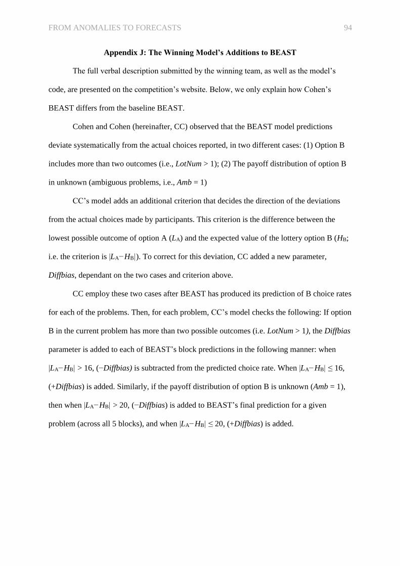
FROM ANOMALIES TO FORECASTS 94
Appendix J: The Winning Model’s Additions to BEAST
The full verbal description submitted by the winning team, as well as the model’s
code, are presented on the competition’s website. Below, we only explain how Cohen’s
BEAST differs from the baseline BEAST.
Cohen and Cohen (hereinafter, CC) observed that the BEAST model predictions
deviate systematically from the actual choices reported, in two different cases: (1) Option B
includes more than two outcomes (i.e., LotNum > 1); (2) The payoff distribution of option B
in unknown (ambiguous problems, i.e., Amb = 1)
CC’s model adds an additional criterion that decides the direction of the deviations
from the actual choices made by participants. This criterion is the difference between the
lowest possible outcome of option A (LA) and the expected value of the lottery option B (HB;
i.e. the criterion is |LA−HB|). To correct for this deviation, CC added a new parameter,
Diffbias, dependant on the two cases and criterion above.
CC employ these two cases after BEAST has produced its prediction of B choice rates
for each of the problems. Then, for each problem, CC’s model checks the following: If option
B in the current problem has more than two possible outcomes (i.e. LotNum > 1), the Diffbias
parameter is added to each of BEAST’s block predictions in the following manner: when
|LA−HB| > 16, (−Diffbias) is subtracted from the predicted choice rate. When |LA−HB| ≤ 16,
(+Diffbias) is added. Similarly, if the payoff distribution of option B is unknown (Amb = 1),
then when |LA−HB| > 20, (−Diffbias) is added to BEAST’s final prediction for a given
problem (across all 5 blocks), and when |LA−HB| ≤ 20, (+Diffbias) is added.

FROM ANOMALIES TO FORECASTS 95
If a problem has more than two possible outcomes and is also an ambiguous problem,
Diffbias is added and/or subtracted (depending on the level of the criterion) both times. Thus,
the process of adding or subtracting the parameter is serial and independent. For example, in
Problem 69, LotNum > 1 and Amb = 1. Because for this problem |LA−HB| = |11−31| = 20, the
first rule subtracts (−Diffbias) and then the second rule adds (+Diffbias).
The parameter Diffbias is a property of the agent, and is assumed to be drawn from a
uniform distribution between 0 and Diffbias: Diffbiasi ~ Uni(0, Diffbias). Best fit of the
Calibration set was obtained with Diffbias = 0.07.

FROM ANOMALIES TO FORECASTS 96
Appendix K: Descriptions of models not statistically inferior to the winner
Model
ID
Rank Prediction
MSD
Problems
Better
Short description
DB49 2 0.0093 28 BEAST with the additional assumptions that (a)
in trivial problems the error term is small but
positive, (b) pBias does not change after more
than 10 trials with feedback, (c) the Sign tool is
used twice as often as the other biased tools,
and (d) the estimates of the model’s parameters
are slightly different (smaller Κ and ψ, larger σ
and β).
EK8 3 0.0093 28 In the absence of feedback, uses BEAST. When
feedback is available, uses IBL with initial
expectations (“prepopulated instances”) based
on BEAST.
DS24 4 0.0096 27 BEAST with increased attractiveness for the
option with the higher maximal gain in the gain
domain, or the lower minimal loss in the loss
domain. Additionally, slightly delayed effect for
feedback, increased aversion for symmetric
mixed gambles compared to certain outcomes,
and some noise in the first two blocks when
predictions are extreme.
NS50 5 0.0096 27 BEAST, with faster convergence towards using
the unbiased tool. Additionally, replacement of
the uniform tool with a pessimistic heuristic
likely to give more weight to minimal
outcomes, and changes to relative probabilities
of using the biased tools.
MK51 6 0.0096 24 BEAST with changes to relative probabilities of
using biased tools (usually less use of the
uniform tool)
BEAST NA 0.0098 24 See main text
DA45 7 0.0098 26 BEAST with increased pessimism for
ambiguous problems.
BS53 8 0.0103 30 BEAST with a chance of using mental draw
(luck-level) for the unbiased tool even after
obtaining feedback. Additionally, sensitivity to
sequences of outcomes in ambiguous problems
and small but positive error in trivial problems.
MS20 9 0.0106 25 In the absence of feedback, uses BEAST. When
feedback is available, uses a weighted average

FROM ANOMALIES TO FORECASTS 97
of BEAST and win-stay-lose-shift strategy.
OY42 11 0.0107 18 In the absence of feedback, uses BEAST. When
feedback is available, uses either BEAST or a
strategy selecting the option providing higher
payoff in a few recent trials (equally likely).
Additionally, uses diminishing sensitivity for
outcomes in all cases.
SH23 12 0.0115 22 BEAST, with changes to sampling tools: (a) the
unbiased tool replaced with draw from
distribution function with probabilities
transformed as in CPT; (b) with feedback, the
uniform tool draws from actual observed
outcomes (as in BEAST’s unbiased); and (c)
with feedback, contingent pessimism sometimes
becomes optimism (maximin). Additionally, Κ
= 1 and the probability of using the new
“unbiased” tool converges slower.
GN27 13 0.0124 26 A support vector regression with 24–28 features
per block per problem including: most of the
problem’s defining parameters; the differences
between the EVs assuming unbiased
distributions, assuming outcomes are equally
likely, assuming the outcomes are sign-
transformed, and assuming the distributions are
transformed as in CPT; the probability of one
option generating better outcome than the other;
SignMax and RationMin (as in BEAST); the
prediction of a stochastic version of CPT; the
difference between the options’ variances; the
difference between the options’ entropies; the
sign of the majority of the possible outcomes;
and the model’s predictions for the previous
blocks. In ambiguous problems, where relevant,
uses BEAST mechanisms to get features’
values. Additionally, the prediction is weighted
with that of stochastic CPT when the problem is
considered particularly difficult or with perfect
maximization when it is particularly easy
(trivial).
WH9 14 0.0127 28 A weighted average of two models. One first
classifies the problem into one of seven classes
and then provides predictions based on a log-
linear model. A problem’s class depends on the
number of outcomes in each option and on their
sign. In each class, the log-linear model uses

FROM ANOMALIES TO FORECASTS 98
one or more of the following as explanatory
variables: the EV; the probability of the option
generating better outcome than the other; the
value, sign, and probability of the maximal
outcome; the sign of the minimal outcome; the
expected rank of an obtained outcome relative
to all possible outcomes; the sum of cues in
which the option is better than the other (cues
are EV, expected rank, maximal and minimal
outcomes, possible regret, and probability of
maximum). The second model is a stochastic
version of CPT where probabilities in
ambiguous problems are considered equally
likely, very small probabilities are neglected,
probabilities are slightly skewed towards
uniform, and updating of probabilities to be
perceived as more extreme with feedback.
Additionally, dominant options are
automatically chosen.
Note. Only submitted models for which a bootstrap analysis of the test set problems suggests they are not
statistically inferior (according to their MSD) to the competition’s winner are listed. Rank refers to the official
ranking in the competition, based on the prediction MSD. Problems Better refers to the number of problems in
the test set (of 60 possible) in which the model provides a better prediction than the competition’s winner.

FROM ANOMALIES TO FORECASTS 99
Appendix L: Analysis of BEAST’s Features Using Random Forest
We have identified 13 features that capture the essence of the baseline model BEAST
(see Plonsky, Erev, Hazan, & Tennenholtz). The first two features, dBEV0 and dBEVFB,
capture the differences between the two options’ BEVs (best estimate of expected values) as
implied by BEAST. Two features are required because BEAST assumes an ambiguous
option’s BEV changes with feedback. Specifically,
0
, 0
/ 3 , 1
B A
B B A A
EV EV AmbdBEV
Min UEV EV EV Amb
, 0
1/ 3 , 1
2
B A
FB
B B A B A
EV EV Amb
dBEVMin UEV EV EV EV Amb
Two additional features capture the logic of sampling using the unbiased tool. It
should be noted that the average outcome drawn using this tool is already captured by the
first two features, but using this tool also implies sensitivity to the probability that one option
will generate a higher outcome than the other (i.e., probability of immediate regret in
choosing the alternative). Again, two features are required because BEAST assumes different
abstractions of this tool before and with feedback. The first feature, pBetter0, equals the
difference between the probability that Option B generates the better outcome when sampling
according to the luck-level procedure and the probability that Option A generates the better
outcome with this procedure. The second feature, pBetterFB, equals the same difference,
except that instead of using luck-level, the draw is made from the observed outcomes (thus, it
is sensitive to the correlation between the outcomes).
The next two features capture the use of the uniform sampling tool. The first feature,
pBetterUni, equals the difference between the probability B generates the better outcome when
sampling using the uniform tool and the probability that A generates the better outcome when
sampling using this tool. The second feature, dUniEV, captures the average outcomes drawn

FROM ANOMALIES TO FORECASTS 100
using this tool. It equals the difference between the options’ EVs after their distributions are
transformed to uniform distributions.
Three other features capture sampling using the sign tool. dSignEV equals the
difference between the options’ EVs after they are transformed according to the sign tool.
The two other features, pBetterSign0 and pBetterSignFB, capture the differences between the
probabilities of drawing a better outcome in B and those of drawing a better outcome in A,
before and with feedback (similarly to the pBetter0 and pBetterFB).
The next three features capture the contingent pessimism tool. The first, dMins, equals
the difference between the options’ minimal outcomes. The other two features capture the
conditions under which BEAST assumes this tool is not used. Specifically, RatioMin is
computed as in Equation (2) in the main text, whereas SignMax equals the sign of the
maximal possible outcome in that problem. The final feature captures the sensitivity of
BEAST’s error term to the presence of dominant options. The feature Dom equals 1 if Option
B dominates Option A, -1 if A dominates B, and 0 otherwise.
In addition to these 13 features, a block feature (equals 1,2,…5) was supplied as input
to the Random Forest algorithm. This was done to allow the algorithm to differentiate
between the five different blocks generated by each of the 90 problems of the training set,
and to allow it to produce different predictions for the different blocks in the test set.
Implementing the algorithm with all these features implies an MSD score of 0.0098 on the
test set, virtually identical to the MSD of BEAST.
Next, we ran the algorithm 13 additional times, each time removing one of the
psychological features described above. The results suggest that all 13 algorithms have
similar predictive power on the test set. Their MSDs ranged between 0.0093 and 0.0113.
Notice, however, that many of the features are very highly correlated (e.g., the correlation
between dBEV0 and dBEVFB is 0.93) and therefore removal of one of the features may not

FROM ANOMALIES TO FORECASTS 101
have greatly affected the algorithm’s performance because another feature compensated for
its absence.
To obtain a clearer picture of the importance of BEAST’s mechanisms, we re-
evaluated the algorithm’s performance after removing sets of features, each capturing a
different mechanism of BEAST. Specifically, running the algorithm without either dBEV0 or
dBEVFB – that is without assuming sensitivity to the best estimates of the expected values –
implies an MSD score of 0.0168, a 72% decrease in the predictive performance relative to the
baseline that includes this mechanism. Running the algorithm without either pBetter0 or
pBetterFB – that is without assuming a tendency to minimize immediate regret – implies an
MSD score of 0.0156, a 59% decrease in the algorithm’s relative predictive performance.
These results highlight the importance of including both mechanisms for a model to provide
useful predictions for the current data.
In contrast, removal of each of the three sets of features that capture the use of each of
the biased sampling tools does not lead to a great decrease in predictive performance.
Specifically, removal of the two uniform features leads to MSD of 0.0104; removal of the
three sign features leads to MSD of 0.0109; and removal of the three contingent pessimism
features leads to MSD of 0.0105. However, this does not mean that the use of biased
sampling tools is unwarranted. Indeed, removal of all eight features that capture the use of
these biased tools implies an MSD score of 0.0162, a 66% decrease in the model’s relative
predictive performance. Therefore, while it may be possible to provide useful predictions
with different abstractions of biased sampling tools (that correspond to certain behavioral
tendencies), BEAST correctly captures the importance of incorporating such biases. One
advantage of BEAST over the abstractions implied by the various Random Forest algorithms
is its relative interpretability.

FROM ANOMALIES TO FORECASTS 102
Finally, running the algorithm without the Dom feature leads, surprisingly, to slightly
better predictive power: It implies MSD of 0.0094. It seems that BEAST’s assumption of a
completely different error mechanism for “trivial” games is too strong.