RPSEA - National Energy Technology Laboratory library/research/oil-gas/deepwater... · RPSEA FINAL...

RPSEA

FINAL TECHNICAL REPORT

Document Number: 08121-2902-07.FINAL

Fiber-containing Sweep Fluids for Ultra Deepwater Drilling Applications

Contract Number: 08121-2902-07

March 3, 2012

Ramadan M. Ahmed

Assistant Professor

The University of Oklahoma

100 Boyd St., Norman, OK 73019

ii

LEGAL NOTICE

This report was prepared by The University of Oklahoma as an account of work sponsored by

the Research Partnership to Secure Energy for America, RPSEA. Neither RPSEA members of

RPSEA, the National Energy Technology Laboratory, the U.S. Department of Energy, nor any

person acting on behalf of any of the entities:

a. MAKES ANY WARRANTY OR REPRESENTATION, EXPRESS OR IMPLIED WITH

RESPECT TO ACCURACY, COMPLETENESS, OR USEFULNESS OF THE INFORMATION

CONTAINED IN THIS DOCUMENT, OR THAT THE USE OF ANY INFORMATION,

APPARATUS, METHOD, OR PROCESS DISCLOSED IN THIS DOCUMENT MAY NOT

INFRINGE PRIVATELY OWNED RIGHTS, OR

b. ASSUMES ANY LIABILITY WITH RESPECT TO THE USE OF, OR FOR ANY AND ALL

DAMAGES RESULTING FROM THE USE OF, ANY INFORMATION, APPARATUS,

METHOD, OR PROCESS DISCLOSED IN THIS DOCUMENT.

THIS IS AN INTERIM REPORT. THEREFORE, ANY DATA, CALCULATIONS, OR CONCLUSIONS

REPORTED HEREIN SHOULD BE TREATED AS PRELIMINARY.

REFERENCE TO TRADE NAMES OR SPECIFIC COMMERCIAL PRODUCTS, COMMODITIES, OR

SERVICES IN THIS REPORT DOES NOT REPRESENT OR CONSTIITUTE AND ENDORSEMENT,

RECOMMENDATION, OR FAVORING BY RPSEA OR ITS CONTRACTORS OF THE SPECIFIC

COMMERCIAL PRODUCT, COMMODITY, OR SERVICE.

iii

Abstract

This report presents experimental and theoretical studies conducted on the rheology and stability of fiber-

containing sweep fluids. In addition, the report shows results of our investigations on settling behavior of

solids particles in fiber sweeps. Spherical glass particles with different diameters were used. We

performed experiments using water and oil-based fluids. Fluid composition and fiber concentration were

varied during the investigation.

Rheological properties of the fluid samples were measured before stability and settling velocity

experiments. Even though 0.04 percent fiber content is recommended in the field for sweep application,

tests were conducted varying fiber content from 0.00 to 0.08 percent. Results indicate the absence of

excessive thickening, which is frequently observed in highly concentrated fiber suspensions. Because of

their low fiber concentration, fiber sweeps are not vulnerable to excessive thickening.

The stability of fiber sweep determined the hole-cleaning performance of the fluid. During our

investigations, we developed mathematical models based on hydrodynamic drag behavior of long

cylinders. They predict the stability of non-Newtonian fiber suspensions. Model predictions showed good

agreement with experimental results. Both theoretical analysis and experimental observation suggested

the critical role of viscosity in maintaining the stability of the fluid. Highly viscous base fluids created

stable fiber suspensions. However, viscosity was not the only parameter that controlled the stability of

these fluids. The polymer type also played a great role. In general, xanthan gum-based fluids showed

very good stability. In addition to the polymer type, the existence of structure in the fluid also stabilized

the fluid. Oil-based muds (OBM and SBM) are structured fluids with a continuous oil phase and

dispersed water droplets. Because of the surfactant (i.e., emulsifier), the fluid maintained its structure for

sufficiently long time. The structure trapped fiber particles and kept them in the suspension without

segregation. All oil-based fluids that were tested show excellent stability.

Settling velocity of cuttings is often used to assess hole-cleaning performance of drilling fluids. The

addition of fiber into a drilling fluid substantially reduced the settling velocity of cuttings and improved

carrying capacity of the fluid. The velocity reduction came from the improvement of the drag force that

opposes the motion of the particle. When fiber particles were fully dispersed in the fluid, they tended to

form a network structure that generated additional drag force (fiber drag). After obtaining settling velocity

measurements, we were able to determine the contribution of the fiber drag to the total drag force. Due to

the strong interactions between the fiber particles and the base fluid, the hydrodynamic component of the

fiber drag dominated the drag that originated because of mechanical friction and fiber entanglement. As a

result, the fiber drag was strongly related to viscous properties of the fluid. In this study, we developed a

settling velocity model by predicting settling behavior of particles in fiber sweeps. The model accounted

for the presence of fiber particle using the fiber drag coefficient. Model predictions showed a satisfactory

agreement with experimental measurements.

iv

Sweep experiments were conducted with fiber-containing water-based and synthetic-based drilling fluids

to study wellbore cleaning performance. Extensive flow loop experiments were carried out by varying

fiber concentration (up to 0.27 lb/bbl) in industry utilized water-based and synthetic-based drilling fluid

formulations. Cuttings bed heights in the flow loop annulus were measured at different flow rates and

pipe rotation speeds for the different fluid-fiber combinations at horizontal and inclined configurations. In

addition, to investigate the hydraulic impact of the fiber, pipe viscometer and wellbore hydraulics

experiments were conducted at varying fiber concentrations. Results showed that fiber sweeps

substantially improved cuttings removal compared to the base fluid sweeps, despite similar equivalent

circulating densities.

A mechanistic model was developed to predict critical cuttings transport velocity or equilibrium bed

height in horizontal and inclined wellbores with fiber-containing fluids. The model was developed by

considering fluid flow over a stationary bed of solid particles of uniform thickness. The model required a

correlation for estimating the additional drag (i.e., fiber drag) resulting from the presence of fiber in the

fluid. Settling velocity experimental data was used to provide a correlation for the fiber drag coefficient,

and the sweep experiments were used to verify the model predictions. The critical transport velocity was

measured by visual observation of the cuttings bed particles movement. The model predictions and

experimental measurements showed good agreement at low flow rates. For fluids without fiber (i.e., base

fluid), mechanistic model predictions were compared with published experimental results and with

predictions of an existing model. The comparisons showed satisfactory agreement with measurements and

better accuracy than the existing model.

v

Signature: __________________________ Date: _______March, 03, 2012__________

vii

Table of Contents

Disclaimer

Abstract

Table of Contents

List of Tables

List of Figures

1. Executive Summary

2. Theoretical Study on Stability of Fiber Sweeps

2.1. Particle Settling Behavior

2.1.1. Classification of Particle Settling Behavior

2.1.2. Motion of Fibrous Particles

2.2. Modeling Rising Velocity of Particles

2.3. Non-Rising Particles under Static Conditions

2.4. Non-Rising Particles under Dynamic Conditions

2.5. Modeling Results

2.6. Conclusions

Nomenclature

References

3. Experimental Study on Stability of Fiber Sweeps

3.1. Scope

3.2. Experimental Setup and Procedure

3.3. Results

3.3.1. Effect of Base Fluid Rheology on Stability of Fiber Sweep

3.3.2. Effect of Temperature on Stability of Fiber Sweep

3.3.3. Comparison of Model Predictions with Experimental Results

3.4. Conclusions

Nomenclature

References

4. Rheological Properties of Fiber Sweeps

4.1. Introduction

4.2. Literature Review

4.3. Fiber Fluid Rheology

ii

iii

vii

x

xi

1

4

4

4

5

6

8

11

12

15

16

17

18

18

18

19

20

26

27

28

29

29

30

30

32

34

viii

4.4. Experimental Investigations

4.4.1. Experimental Setup

4.4.2. Test Procedure

4.5. Experimental Results

4.5.1. Effect of Fiber Concentration

4.5.2. Effect of Temperature

4.5.3. Shear Viscosity Parameters

4.6. Conclusions

Nomenclature

References

5. Settling Behavior of Particles in Fiber-containing Drilling Fluids

5.1. Introduction

5.2. Settling in Fiber Suspensions

5.3. Experimental Study

5.3.1. Experimental Setup

5.3.2. Test Materials

5.3.3. Test Procedure

5.3.4. Test Results

5.4. Analysis of Results and Discussions

5.5. Model Predictions

5.6. Conclusions

Nomenclature

References

6. Hole Cleaning Performance of Fiber Sweeps

6.1. Introduction

6.2. Experimental Setup

6.3. Experimental Procedure

6.4. Experimental Test Matrix

6.4.1. WBM Test Matrix

6.4.2. SBM Test Matrix


6.5.1. Dynamic Variation of Cuttings Bed Height

6.5.2. Effect of Fluid Types

36

36

37

38

38

44

45

48

48

49

51

51

55

56

57

58

58

59

62

63

64

65

65

68

68

69

71

76

76

77

78

78

79

ix

6.5.3. Effect of Fiber Concentration

6.5.4. Effect of Inclination Angle

6.5.5. Effect of Flow Rate

6.5.6. Effect of Pipe Rotation

6.6. Pipe Viscometer Measurements

6.7. Wellbore Hydraulics

6.8. Conclusions

6.9. Guidelines

Nomenclature

References

7. Mechanistic Modeling of Hole Cleaning with Fiber Sweeps

7.1. Introduction

7.2. Forces Involved in Particle Transport

7.2.1. Gravity and Buoyancy Forces

7.2.2. Hydrodynamic Forces

7.2.3. Fiber Drag Force

7.2.4. Plastic Force

7.3. Near-Bed Velocity Profile

7.3.1. Newtonian Fluid

7.3.2. Non-Newtonian Fluid

7.4. Mechanistic Model Formulation


7.5.1. Comparison of Model Predictions with Test Measurements

7.5.2. Comparison of Model Predictions with Published Data and Existing Model

7.6. Conclusions

Nomenclature

References

82

85

87

88

89

92

93

94

95

96

97

97

98

99

99

101

102

103

103

103

106

107

107

108

110

110

111

x

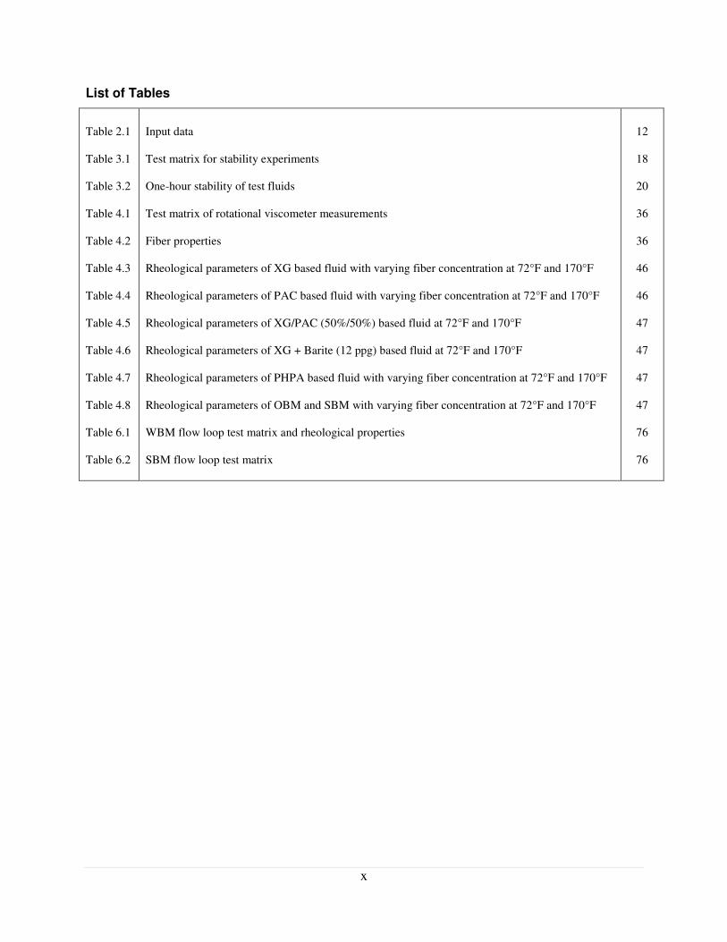
List of Tables

Table 2.1

Table 3.1

Table 3.2

Table 4.1

Table 4.2

Table 4.3

Table 4.4

Table 4.5

Table 4.6

Table 4.7

Table 4.8

Table 6.1

Table 6.2

Input data

Test matrix for stability experiments

One-hour stability of test fluids

Test matrix of rotational viscometer measurements

Fiber properties

Rheological parameters of XG based fluid with varying fiber concentration at 72°F and 170°F

Rheological parameters of PAC based fluid with varying fiber concentration at 72°F and 170°F

Rheological parameters of XG/PAC (50%/50%) based fluid at 72°F and 170°F

Rheological parameters of XG + Barite (12 ppg) based fluid at 72°F and 170°F

Rheological parameters of PHPA based fluid with varying fiber concentration at 72°F and 170°F

Rheological parameters of OBM and SBM with varying fiber concentration at 72°F and 170°F

WBM flow loop test matrix and rheological properties

SBM flow loop test matrix

12

18

20

36

36

46

46

47

47

47

47

76

76

xi

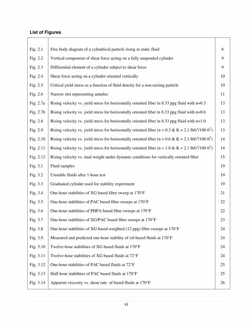
List of Figures

Fig. 2.1

Fig. 2.2

Fig. 2.3

Fig. 2.4

Fig. 2.5

Fig. 2.6

Fig. 2.7a

Fig. 2.7b

Fig. 2.8

Fig. 2.9

Fig. 2.10

Fig. 2.11

Fig. 2.12

Fig. 3.1

Fig. 3.2

Fig. 3.3

Fig. 3.4

Fig. 3.5

Fig. 3.6

Fig. 3.7

Fig. 3.8

Fig. 3.9

Fig. 3.10

Fig. 3.11

Fig. 3.12

Fig. 3.13

Fig. 3.14

Free body diagram of a cylindrical particle rising in static fluid

Vertical component of shear force acting on a fully suspended cylinder

Differential element of a cylinder subject to shear force

Shear force acting on a cylinder oriented vertically

Critical yield stress as a function of fluid density for a non-raising particle

Narrow slot representing annulus

Rising velocity vs. yield stress for horizontally oriented fiber in 8.33 ppg fluid with n=0.3



Rising velocity vs. yield stress for horizontally oriented fiber (n = 0.3 & K = 2.1 lbfsn/100 ft

2)


2)


2)

Rising velocity vs. mud weight under dynamic conditions for vertically oriented fiber

Fluid samples

Unstable fluids after 1-hour test

Graduated cylinder used for stability experiment

One-hour stabilities of XG based fiber sweep at 170°F

One-hour stabilities of PAC based fiber sweeps at 170°F

One-hour stabilities of PHPA based fiber sweeps at 170°F

One-hour stabilities of XG/PAC based fiber sweeps at 170°F

One-hour stabilities of XG based weighted (12 ppg) fiber sweeps at 170°F

Measured and predicted one-hour stability of oil-based fluids at 170°F

Twelve-hour stabilities of XG based fluids at 170°F

Twelve-hour stabilities of XG based fluids at 72°F

One-hour stabilities of PAC based fluids at 72°F

Half-hour stabilities of PAC based fluids at 170°F

Apparent viscosity vs. shear rate of based fluids at 170°F

6

9

9

10

10

11

13

13

13

13

14

14

15

19

19

19

21

22

22

23

24

24

24

24

25

25

26

xii

Fig. 4.1

Fig. 4.2

Fig. 4.3

Fig. 4.4

Fig. 4.5

Fig. 4.6

Fig. 4.7

Fig. 4.8

Fig. 5.1

Fig. 5.2

Fig. 5.3

Fig. 5.4

Fig. 5.5

Fig. 5.6

Fig. 5.7

Fig. 5.8

Fig. 5.9

Fig. 5.10

Fig. 5.11

Fig. 5.12

Fig. 6.1

Fig. 6.2

Fig. 6.3

Fig. 6.4

Fig. 6.5

Fig. 6.6

Fig. 6.7

Fig. 6.8

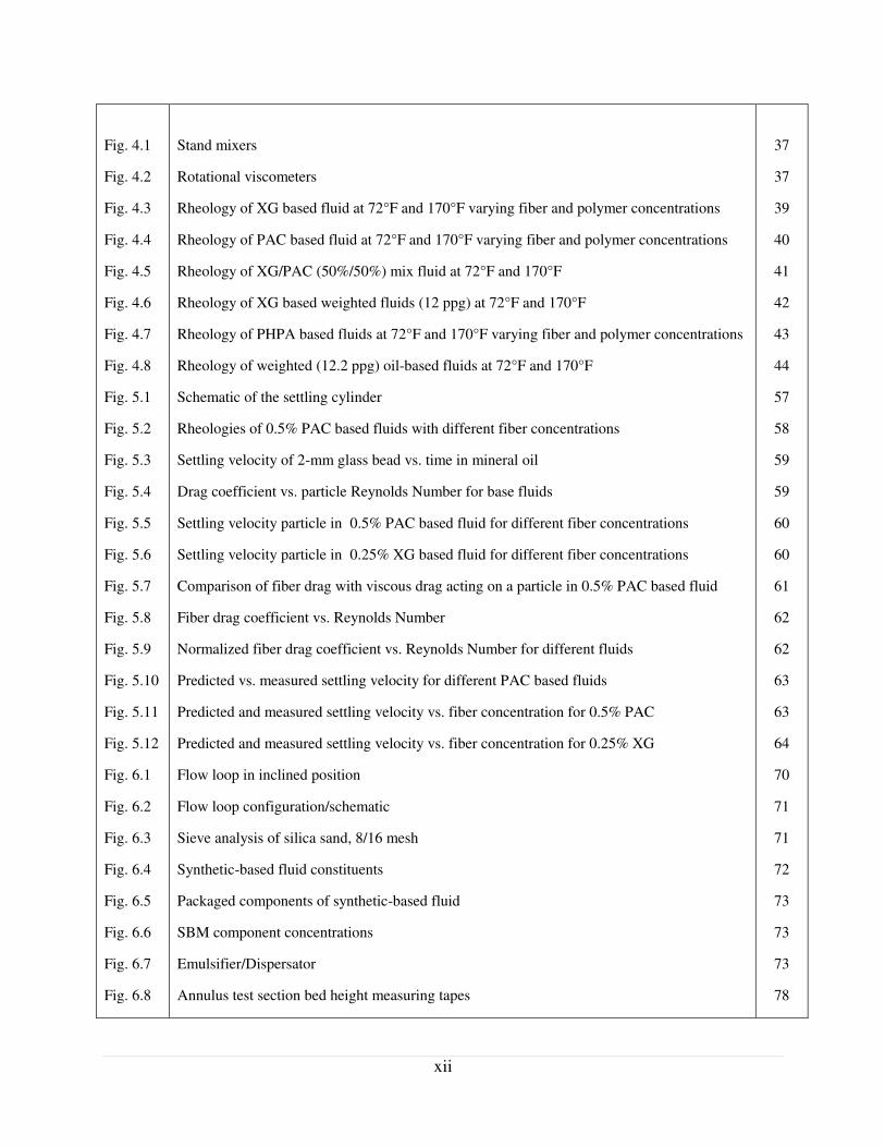
Stand mixers

Rotational viscometers

Rheology of XG based fluid at 72°F and 170°F varying fiber and polymer concentrations

Rheology of PAC based fluid at 72°F and 170°F varying fiber and polymer concentrations

Rheology of XG/PAC (50%/50%) mix fluid at 72°F and 170°F

Rheology of XG based weighted fluids (12 ppg) at 72°F and 170°F

Rheology of PHPA based fluids at 72°F and 170°F varying fiber and polymer concentrations

Rheology of weighted (12.2 ppg) oil-based fluids at 72°F and 170°F

Schematic of the settling cylinder

Rheologies of 0.5% PAC based fluids with different fiber concentrations

Settling velocity of 2-mm glass bead vs. time in mineral oil

Drag coefficient vs. particle Reynolds Number for base fluids

Settling velocity particle in 0.5% PAC based fluid for different fiber concentrations

Settling velocity particle in 0.25% XG based fluid for different fiber concentrations

Comparison of fiber drag with viscous drag acting on a particle in 0.5% PAC based fluid

Fiber drag coefficient vs. Reynolds Number

Normalized fiber drag coefficient vs. Reynolds Number for different fluids

Predicted vs. measured settling velocity for different PAC based fluids

Predicted and measured settling velocity vs. fiber concentration for 0.5% PAC

Predicted and measured settling velocity vs. fiber concentration for 0.25% XG

Flow loop in inclined position

Flow loop configuration/schematic

Sieve analysis of silica sand, 8/16 mesh

Synthetic-based fluid constituents

Packaged components of synthetic-based fluid

SBM component concentrations

Emulsifier/Dispersator

Annulus test section bed height measuring tapes

37

37

39

40

41

42

43

44

57

58

59

59

60

60

61

62

62

63

63

64

70

71

71

72

73

73

73

78

xiii

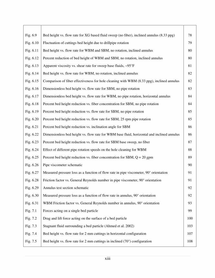
Fig. 6.9

Fig. 6.10

Fig. 6.11

Fig. 6.12

Fig. 6.13

Fig. 6.14

Fig. 6.15

Fig. 6.16

Fig. 6.17

Fig. 6.18

Fig. 6.19

Fig. 6.20

Fig. 6.21

Fig. 6.22

Fig. 6.23

Fig. 6.24

Fig. 6.25

Fig. 6.26

Fig. 6.27

Fig. 6.28

Fig. 6.29

Fig. 6.30

Fig. 6.31

Fig. 7.1

Fig. 7.2

Fig. 7.3

Fig. 7.4

Fig. 7.5

Bed height vs. flow rate for XG based fluid sweep (no fiber), inclined annulus (8.33 ppg)

Fluctuation of cuttings bed height due to drillpipe rotation

Bed height vs. flow rate for WBM and SBM, no rotation, inclined annulus

Percent reduction of bed height of WBM and SBM, no rotation, inclined annulus

Apparent viscosity vs. shear rate for sweep base fluids, ~95°F

Bed height vs. flow rate for WBM, no rotation, inclined annulus

Comparison of fiber effectiveness for hole cleaning with WBM (8.33 ppg), inclined annulus

Dimensionless bed height vs. flow rate for SBM, no pipe rotation

Dimensionless bed height vs. flow rate for WBM, no pipe rotation, horizontal annulus

Percent bed height reduction vs. fiber concentration for SBM, no pipe rotation

Percent bed height reduction vs. flow rate for SBM, no pipe rotation

Percent bed height reduction vs. flow rate for SBM, 25 rpm pipe rotation

Percent bed height reduction vs. inclination angle for SBM

Dimensionless bed height vs. flow rate for WBM base fluid, horizontal and inclined annulus

Percent bed height reduction vs. flow rate for SBM base sweep, no fiber

Effect of different pipe rotation speeds on the hole cleaning for WBM

Percent bed height reduction vs. fiber concentration for SBM, Q = 20 gpm

Pipe viscometer schematic

Measured pressure loss as a function of flow rate in pipe viscometer, 90° orientation

Friction factor vs. General Reynolds number in pipe viscometer, 90° orientation

Annulus test section schematic

Measured pressure loss as a function of flow rate in annulus, 90° orientation

WBM Friction factor vs. General Reynolds number in annulus, 90° orientation

Forces acting on a single bed particle

Drag and lift force acting on the surface of a bed particle

Stagnant fluid surrounding a bed particle (Ahmed et al. 2002)

Bed height vs. flow rate for 2 mm cuttings in horizontal configuration

Bed height vs. flow rate for 2 mm cuttings in inclined (70°) configuration

78

79

80

80

81

82

82

83

84

84

85

85

86

86

87

88

89

90

91

91

92

92

93

99

100

103

107

108

xiv

Fig. 7.6

Fig. 7.7

Bed height vs. flow rate for 0.45 mm cuttings with PAC based fluid

Bed height vs. flow rate for 0.45 mm cuttings with PAC based fluid

109

109

1 | P a g e

1. Executive Summary

Project Management Plan and Technology Status Assessment (Tasks 1 & 2): The project began with

developing the project management plan and assessing the technology status. As required by RPSEA, the

project management plan and technology status assessment report were submitted within 30 days of the

award. The project management plan presents project work breakdown structure, schedules, key

milestones, and planned expenditures for each Task.

Technology Transfer, Project Reporting and Other Activities (Tasks 3 & 4): Different technology

transfer methodologies are being implemented to disseminate the outcomes of the project. Project

outcomes have been presented in different meetings including: Six RPSEA TAC meetings and MPGE

advisory board meeting. A paper on rheology of fiber sweeps (George et al. 2011) was presented at the

2011 AADE meeting. We participated in the 2011 Offshore Technology Conference (OTC), University

showcase. Furthermore, a book chapter (George et al. 2012) and a journal article (Elgaddafi et al. 2012)

have been accepted for publication.

Literature Review and Theoretical Study (Task 5): The research part of the project began with

extensive literature review on fiber-containing fluid systems. Literature review and theoretical

investigations on rheology, hydraulics, stability and carrying capacity of fiber-containing drilling sweeps

were undertaken. The outcomes of this task that are presented in Sections 2, 4, and 5 were used to develop

a mechanistic model to predict the hole cleaning performance of fiber sweeps. The model optimizes fiber

sweep applications.

Bench-Top Experiments (Task 6): These experiments were aimed at developing fiber sweep

formulations that have superior stability and optimum fiber concentration. We developed a stability model

for fiber sweeps and theoretically analyzed their stability (Section 2). This helped us to select the ranges

of base fluid properties that are suitable for fiber sweep applications. The stability of commonly used base

fluids were tested and stable formulations identified (Section 3). Even though excessive thickening is a

common problem with fibrous fluids, our rheology study (Section 4) did not demonstrate the presence of

thickening in fiber sweeps. As the fiber concentration increased, the rheologies of test samples remained

roughly the same. In addition to stability and rheology studies, extensive settling experiments were

carried out (Section 5) to assess carry capacity of fiber sweeps. Based on theoretical analysis and

experimental results, we developed a model that predicts the settling behavior of particles in fiber sweeps.

The model was applied to formulate the mechanistic hole-cleaning model, which was developed in Task

8.

2 | P a g e

Flow Loop Experiments (Task 7): Extensive flow loop experiments were carried out to study rheology,

hydraulics and hole cleaning performance of the base fluids and fiber sweeps. To conduct the

experiments, first the flow loop was modified to perform fiber sweep tests. Fiber concentration,

inclination angle, and pipe rotational speed were varied. Water-based and synthetic-based fluids were

tested. Results showed the hole cleaning performance of the fiber sweep under different conditions.

Mechanistic Modeling (Task 8): Flow loop measurements may not be directly applied to evaluate the

performance of sweep fluid in the field. However, they can be used to validate and calibrate models that

are based on the generalized conservation laws and applicable for both field and lab-scale measurements.

Therefore, in the final stage of the project, modeling study was carried out to formulate a mechanistic that

predicted the performance of the sweep fluid under field conditions and optimized the application of fiber

sweep technology. Flow loop measurements were utilized to evaluate and calibrate the model.

Deliverables of the project:

i. Report and publications presenting:

• Literature review findings (Sections 2.1, 4.2 and 5.1) and data analysis (Sections 3.3, 4.5, 5.4

and 6.4)

• Empirical correlations and semi-empirical models (Section 5.4)

• Mathematical models (Sections 7, 5.2 and 2.2), and

• Mechanisms and physical phenomena involved in the application of fiber sweep (Sections

2.1, 3, 4.1 and 5.1)

ii. Formulations of stable fiber-containing sweep fluids (Section 3.3)

iii. Experimental data describing

• Particle settling velocity (Section 5.3)

• Fiber drag (Section 5.4)

• Rheology and stability under different temperature conditions (Sections 3 and 4)

• Hydraulics and hole cleaning performance of fiber sweeps (Section 6)

iv. Recommendations and guidelines for field applications (Section 6.9)

References

George, M., Ahmed, R. and Growcock, F. 2011.Rheological Properties of Fiber-Containing Drilling

Sweeps at Ambient and Elevated Temperatures, paper AADE-11-NTCE-35, presented at the

AADE National Technical Conference and Exhibition, Houston, Texas, April 12-14, 2011.

3 | P a g e

George, M., Ahmed, R. and Growcock, F. 2012. Stability and Flow Behavior of Fiber-Containing

Drilling Sweeps, Rheology, InTech, Rijeka, Croatia, ISBN: 978-953-51-0187-1,

http://www.intechopen.com/books/rheology/stability-and-flow-behavior-of-fiber-

containing-drilling-sweeps.

Elgaddafi, R., Ahmed, R., George, M. and Growcock, F. 2012. Settling behavior of spherical particles in

fiber-containing drilling fluids, J. Pet. Sci. Eng. (2012), doi:10.1016/j.petrol.2012.01.020.

4 | P a g e

2. Theoretical Study on Stability of Fiber Sweeps

One of the major areas of concerns in the development of fiber sweep technology is fluid instability under

borehole conditions. A recent experimental study (Ahmed and Takach 2008) demonstrated the presence

of fiber separation in low-viscosity sweep fluids. Fiber particle separate or rise in the fluid due to the

buoyant nature of the particles. The separation of the fiber particle substantially reduces the performance

of the sweep fluid.

2.1 Particle Settling Behavior

In contrast to the manufacturing industry, where fiber suspensions are common, the conditions to which

the sweep fluids are subjected can be extremely severe. Modern technological advances within the oil and

gas industry have taken some of the unpredictability out of the well construction phase. Despite this, there

is still no ability to attenuate the harsh environmental conditions that exist within the wellbore, such as

high temperature and high pressure, which necessitate the use of thermally stable, high specific gravity

fluids. These circumstances, unique to the oil and gas industry, and other intangibles, preclude a large

majority of previous work on the flow behavior of homogeneous, non-Brownian suspensions within a

controlled environment. Another dissimilarity is the relative specific gravities of the suspended particles

and the suspending medium. There is a large quantity of experimental, mathematical, and numerical

studies on the settling behavior of spherical and non-spherical particles. However, in the case of fiber

sweeps, the relative gravities are reversed, as the specific gravities of the synthetic fiber and sweep fluid

is less than and greater to water, respectively. This relation encourages buoyancy, and the fibers tend to

rise within the suspension. Despite the opposing directions of motion, the fibers and fiber networks still

exhibit similar general motion and phenomena.

2.1.1 Classification of Particle Settling Behavior

The settling behavior of particles can be divided into four generally accepted classifications, whose

definitions can be revised to reflect the purpose of this study (Scholz 2006):

• Class I: Unhindered settling of discrete particles. The singular particle undergoing this settling

behavior will accelerate until a terminal settling velocity is reached, where the hydrodynamic

drag and gravitational force are balanced. Stokes’ Law is commonly used to describe this motion

of spherical particles.

• Class II: Settling of a dilute suspension of flocculent particles. The randomly moving particles

collide and become entangled, and form aggregates (flocs), which can have increased settling

velocities compared to a single fiber.

• Class III: Hindered and zone settling. Particle concentration is increased to a point where

5 | P a g e

discrete settling no longer occurs. All particles consolidate and displace the liquid phase, which

gives rise to a new upward flow of liquid. This reciprocal motion reduces the overall particle

settling velocity and is called hindered settling. In large surface area settling applications with

high particle concentration, the whole suspension may tend to settle as a “blanket” (zone settling).

• Class IV: Compression settling (compaction and consolidation). As the settling continues, a

compressed layer forms at the bottom of the settling column. As the compression layer is created,

a concentration gradient forms extending upward from the lower sludge region to an increasingly

dilute solids particle concentration.

2.1.2 Motion of Fibrous Particles

Class I and II can be used to describe the motion of synthetic fibers within a low concentrate suspension.

The modeling study considers Class I motion, which simply describes the forces and rising velocity of a

single fiber suspended in a fluid. This prediction can be extrapolated to determine the rising velocity of a

dilute suspension of fiber particles, or Class II motion. Due to the minimal scale of this research, hindered

or zonal settling is readily apparent. While the fibers do rise to the surface of the test cylinders within the

extents of the experiments, there is no true compaction or compression of the fibers at the liquid surface.

The settling motion of a particle is simply a classification of its motion. The settling motion of a fibrous

particle is much more complex (Qi et al. 2011). In the absence of extraneous forces, a sphere settles in a

purely vertical direction. The inconsistent, asymmetrically shaped flexible fiber suspended in a fluid can

exhibit profligate behavior in three dimensions, as well as drift horizontally during its vertical

ascent/descent (Herzhaft and Guazzelli 1999). The rising velocity of these fibers also depends on the fiber

concentration and orientation of the high-aspect ratio particles. Experimental studies investigating dilute

and semi-dilute cylindrical or spheroid particles indicate that concentration is vital in understanding the

settling behavior (Qi et al. 2011; Kuusela et al. 2001, 2003; Koch and Shaqfeh 1989; Herzhaft et al. 1996,

1999). The overall consensus regarding the settling behavior of fiber suspensions was the ability of the

fiber flocs to settle faster than an individual fiber. As the fiber concentration increased, the fibers actually

exhibited hindered settling, and the mean velocity actually decreased below that of a single fiber.

The previous studies mentioned were concerned with phenomena of a similar nature and relevant to this

work. However, due to the particular focus of this study, the ideas and conclusions gathered from

literature must be extrapolated and generalized to correlate to the rising tendency of the fibers. This study

showed rising velocities of fiber particles within a suspension, based on theoretical models and

experimental results.

6 | P a g e

2.2 Modeling Rising Velocity of Particles

The purpose of this modeling study was to predict the behavior of the synthetic monofilament fiber

suspended in fluids with varying rheological properties. In order for the fiber to perform as efficiently and

effectively as possible, the fluid suspending the fiber was engineered to promote the fiber’s wellbore

cleaning capabilities. Thus, a theoretical study was conducted to determine the desirable base fluid

properties and formulate sweep fluids that are stable under borehole conditions.

For the sake of simplicity and to provide easier comparison between fibers oriented perpendicular

(horizontally) and parallel (vertically) to the direction of motion, the analysis only considered a single

fiber suspended in the fluid (Class I settling behavior). This assumption ignored the effect of fiber-fiber

interaction and fiber concentration. The fiber-fiber interaction phenomenon and the fiber concentration in

the fluid were shown to influence the stability of the fiber-fluid system (Ahmed and Takach 2008). This

analysis also addressed two orientations of the fiber: perpendicular to the direction of motion of the fiber

(horizontal) and parallel to the direction of motion of the fiber (vertical). These orientations represent the

boundaries within which the fiber can theoretically orient. However, it has been shown that single settling

fiber will orient itself horizontally (Fan et al. 2004; Kuusela et al. 2001, 2003; Qi et al. 2011). This stable

orientation is also irrespective of fluid velocity, and will eventually return to the horizontal position if

acted upon by an outside force (Qi et al. 2011). Liu and Joseph (1993) investigated how a slender particle

is affected by liquid properties, particle density, length, and shape. They found that only particle

concentration and the end shapes influenced particle orientation during settling. This agrees with studies

by Herzhaft et al. (1996, 1999), which concluded that orientation of a settling spheroid is almost

independent of aspect ratio, but it is correlated to suspension concentration.

As the fiber concentration is increased, the hydrodynamic interactions between the fibers will upset the

stable horizontal fiber. With increasing fiber concentration, the fiber will show greater tendency to orient

parallel toward the direction of motion (Herzhaft et al. 1996; Qi et al. 2011). By analyzing both cases,

we predicted the rheological properties of the base fluid that can keep the fiber in suspension for a

sufficient length of time.

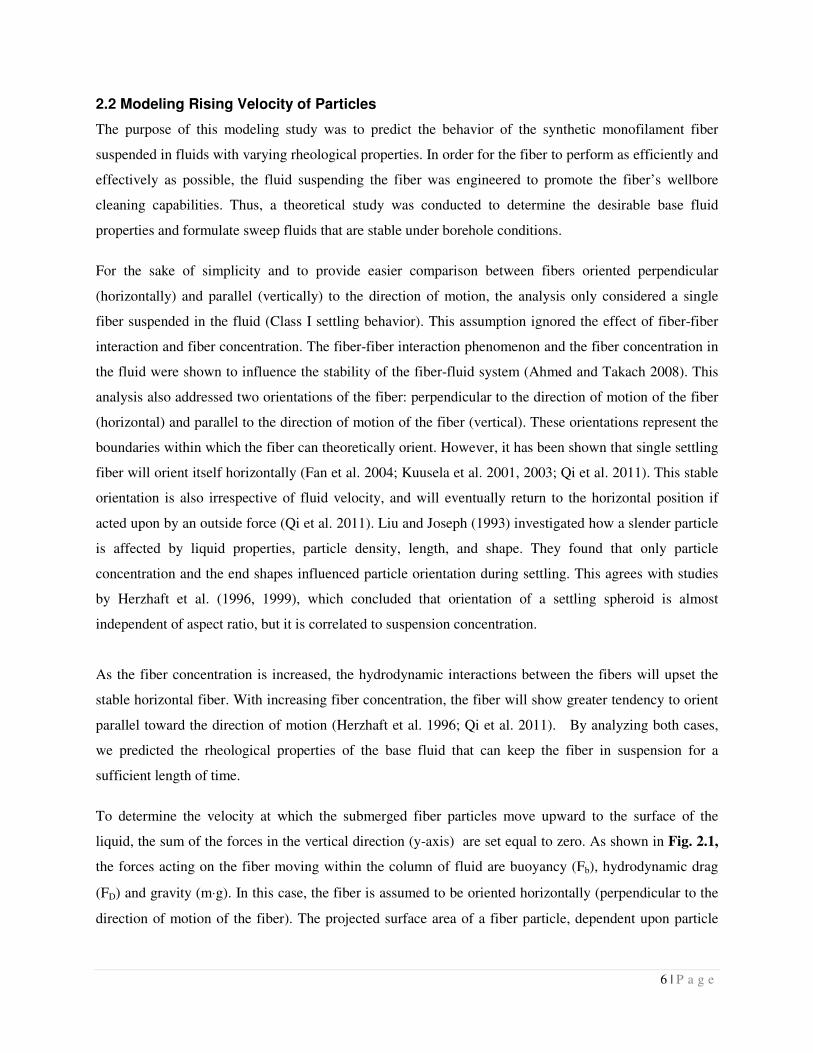
To determine the velocity at which the submerged fiber particles move upward to the surface of the

liquid, the sum of the forces in the vertical direction (y-axis) are set equal to zero. As shown in Fig. 2.1,

the forces acting on the fiber moving within the column of fluid are buoyancy (Fb), hydrodynamic drag

(FD) and gravity (m⋅g). In this case, the fiber is assumed to be oriented horizontally (perpendicular to the

direction of motion of the fiber). The projected surface area of a fiber particle, dependent upon particle

7 | P a g e

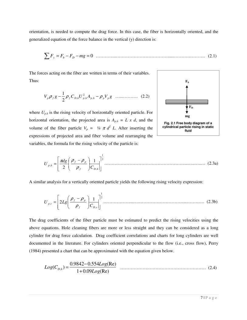
orientation, is needed to compute the drag force. In this case, the fiber is horizontally oriented, and the

generalized equation of the force balance in the vertical (y) direction is:

0=−−=∑ mgFFF Dby …………..………………………………...…………………. (2.1)

The forces acting on the fiber are written in terms of their variables.

Thus:

gVAUCgV pphphphDffp ρρρ −− ,2

,,2

1 …...………. (2.2)

where Up,h is the rising velocity of horizontally oriented particle. For

horizontal orientation, the projected area is Ap,h = L x d, and the

volume of the fiber particle Vp = ¼ π d2 L. After inserting the

expressions of projected area and fiber volume and rearranging the

variables, the formula for the rising velocity of the particle is:

2

1

,

,

1

2

−=

hDf

pf

hpC

dgU

ρ

ρρπ………………………………………………...…..…..… (2.3a)

A similar analysis for a vertically oriented particle yields the following rising velocity expression:

2

1

,

,

12

−=

vDf

pf

vpC

LgUρ

ρρ………………...….…………………………...………… (2.3b)

The drag coefficients of the fiber particle must be estimated to predict the rising velocities using the

above equations. Hole cleaning fibers are more or less straight and they can be considered as a long

cylinder for drag force calculation. Drag coefficient correlations and charts for long cylinders are well

documented in the literature. For cylinders oriented perpendicular to the flow (i.e., cross flow), Perry

(1984) presented a chart that can be approximated with the equation given below.

(Re)09.01

(Re)554.09842.0)( ,

Log

LogCLog hD

+

−= ……………….………………………………… (2.4)

FD

mg

Fb

Fig. 2.1 Free body diagram of a cylindrical particle rising in static

fluid

8 | P a g e

This correlation is valid for Reynolds Numbers (Re) ranging from 10-3 to 10. It has been used extensively

in this study, as most lab experiments involving fibers primarily exist in a Reynolds Number range less

than 1.

The drag coefficient of a cylinder oriented in the direction of the flow is only a function of the aspect ratio

(L/d). Based on available data in the literature (Hoerner 1965), the following equation has been developed

to estimate the drag coefficient, CDv:

23.4,

54.1

/1

317.0825.0

+

+=dl

C vD ………………….…….………………………………… (2.5)

As shown in Eqn. (2.4), the drag coefficient of a cylindrical fiber under cross flow condition is a function

of the Reynolds number, which is generally expressed as Re = ρUp,hd/µ (i.e., the ratio of inertial force to

viscous force). This definition holds true for Newtonian fluids, which possess a linear relationship

between shear stress and shear rate. However, the fluids that are often utilized in fiber sweep applications

are non-Newtonian. Hence, the Reynolds Number needs to be redefined using the apparent viscosity

function as Re = ρUp,hd/µapp. The viscosity for Newtonian fluids is an actual property of the fluid, and is

constant despite the shear rate. However, for non-Newtonian fluids, the apparent viscosity varies with

shear rate and rheological parameters of fluid. Applying the Yield Power Law (YPL) rheology model, the

apparent viscosity, µapp, is expressed as:

( ) ( ) 11 −−+= γτγµ &&

y

n

app K ……………………………..…………………….………...…… (2.6)

This study is to determine the desirable Yield Power Law (YPL) fluid properties that must keep the fiber

in suspension in order to create efficient momentum transfer mechanisms between the sweep fluid and

cuttings bed. Hence, only fluids with sufficient yield stress and/or increased low shear rate viscosity can

be utilized to keep the fibers in suspension.

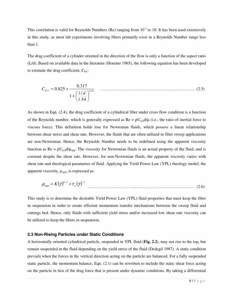
2.3 Non-Rising Particles under Static Conditions

A horizontally oriented cylindrical particle, suspended in YPL fluid (Fig. 2.2), may not rise to the top, but

remain suspended in the fluid depending on the yield stress of the fluid (Dedegil 1987). A static condition

prevails when the forces in the vertical direction acting on the particle are balanced. For a fully suspended

static particle, the momentum balance, Eqn. (2.1) can be rewritten to include the static shear force acting

on the particle in lieu of the drag force that is present under dynamic conditions. By taking a differential

9 | P a g e

element of the cylindrical fiber, the vertical component of the maximum static shear stress (i.e., yield

stress) acting on the fiber can be determined (Fig. 2.2). The direction of the shear stress acting on the

cylinder depends on the location of the differential element as shown in Fig. 2.2. The stress acts on the

area represented by the differential element shown in Fig. 2.3 is expressed as:

θLRddA = ………….………………….………........ (2.7)

Then, the vertical component of the shear force acting on the

differential element is:

θτθθτ sinsin yyshear LRddAdF ⋅=⋅= ……...……. (2.8)

In a fiber oriented vertically and horizontally, shear stresses act on

the circumferential and end areas. However, the end areas are

negligible when compared to circumferential area of the cylinder.

This further simplifies the analysis. Neglecting the forces acting on the cylinder ends, the overall vertical

component of the shear force is subsequently obtained by integrating Eqn. (2.8). After simplification, the

vertical component of the stress force acting on horizontally oriented cylinder becomes:

yhs dLF τ2, = ………….......……………………………………………………...……….. (2.9)

The above equation predicts the maximum value of the

shear force acting on the cylinder. For the sake of

simplicity, the analysis is only concerned with a single

fiber suspended in fluid. The cylinder is considered to

be non-rotating and constantly perpendicular to the

direction of motion of the fiber. In addition, as stated

earlier, the calculations ignore the fiber-fiber

interactions, which will influence the momentum

balance. Writing the force balance in the vertical

direction and replacing the drag force with the shear force in Eqn. (2.1), we get:

gVdLgVF ppyfpy ρτρ −−==∑ 20 ………..………………..…................................. (2.10)

Fig. 2.3 Differential element of a cylinder subject to shear force

Fig. 2.2 Vertical component of shear force acting on a fully

suspended cylinder

10 | P a g e

Replacing the particle volume Vp with πd2L/4, and grouping like terms results in:

( ) 08

2 =

−− ypf

dgdL τρρ

π …………………..…………………………..…………… (2.11)

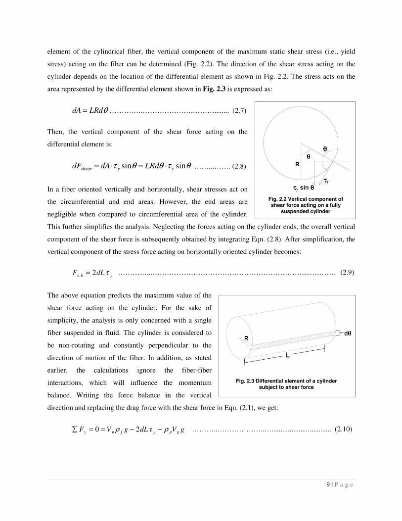
For a fiber particle oriented in the vertical direction (Fig. 2.4), the shear stress acts vertically along the

length of the fiber particle. By taking a circular differential element of height (dh) and circumference

(πd), the shear force can be written as:

y

L

yvs dLdhdF τπτπ == ∫0, …………….……… (2.12)

Once again rewriting the force balance equation to include the

shear force acting on a vertical oriented particle, and grouping

like terms results in:

( )[ ] 044

=−− ypfdgdL

τρρπ

…...……..……... (2.13)

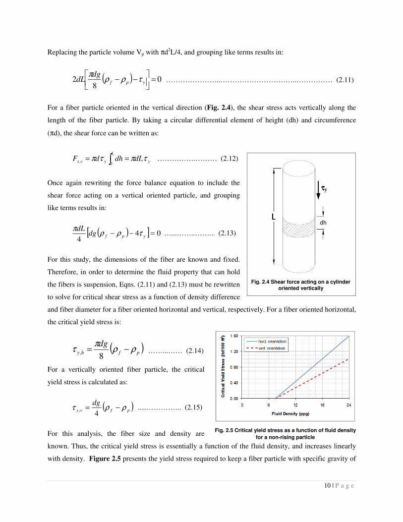
For this study, the dimensions of the fiber are known and fixed.

Therefore, in order to determine the fluid property that can hold

the fibers is suspension, Eqns. (2.11) and (2.13) must be rewritten

to solve for critical shear stress as a function of density difference

and fiber diameter for a fiber oriented horizontal and vertical, respectively. For a fiber oriented horizontal,

the critical yield stress is:

( )pfhy

dgρρ

πτ −=

8, ……...…… (2.14)

For a vertically oriented fiber particle, the critical

yield stress is calculated as:

( )pfvy

dgρρτ −=

4,

......………….. (2.15)

For this analysis, the fiber size and density are

known. Thus, the critical yield stress is essentially a function of the fluid density, and increases linearly

with density. Figure 2.5 presents the yield stress required to keep a fiber particle with specific gravity of

Fig. 2.5 Critical yield stress as a function of fluid density

for a non-rising particle

ττττy

Fig. 2.4 Shear force acting on a cylinder oriented vertically

11 | P a g e

0.9, length of 10 mm, and diameter of 100 µm vertically oriented. Theoretically, very small yield stress

(less than 1.5 lbf/100 ft2) is needed to keep the fiber in suspension.

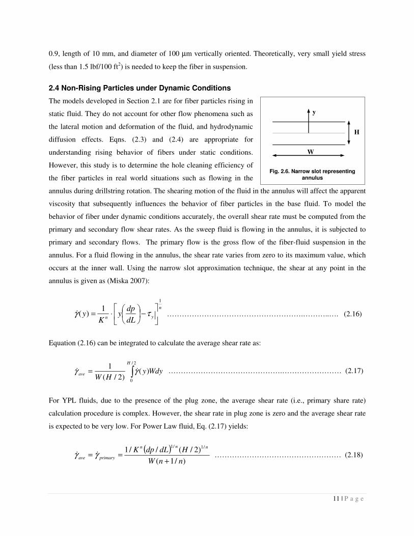
2.4 Non-Rising Particles under Dynamic Conditions

The models developed in Section 2.1 are for fiber particles rising in

static fluid. They do not account for other flow phenomena such as

the lateral motion and deformation of the fluid, and hydrodynamic

diffusion effects. Eqns. (2.3) and (2.4) are appropriate for

understanding rising behavior of fibers under static conditions.

However, this study is to determine the hole cleaning efficiency of

the fiber particles in real world situations such as flowing in the

annulus during drillstring rotation. The shearing motion of the fluid in the annulus will affect the apparent

viscosity that subsequently influences the behavior of fiber particles in the base fluid. To model the

behavior of fiber under dynamic conditions accurately, the overall shear rate must be computed from the

primary and secondary flow shear rates. As the sweep fluid is flowing in the annulus, it is subjected to

primary and secondary flows. The primary flow is the gross flow of the fiber-fluid suspension in the

annulus. For a fluid flowing in the annulus, the shear rate varies from zero to its maximum value, which

occurs at the inner wall. Using the narrow slot approximation technique, the shear at any point in the

annulus is given as (Miska 2007):

n

yn dL

dpy

Ky

1

1)(

−

⋅= τγ& ……………………………………………….………..…. (2.16)

Equation (2.16) can be integrated to calculate the average shear rate as:

∫=2/

0

)()2/(

1H

ave WdyyHW

γγ && ……………………………………….…………………… (2.17)

For YPL fluids, due to the presence of the plug zone, the average shear rate (i.e., primary share rate)

calculation procedure is complex. However, the shear rate in plug zone is zero and the average shear rate

is expected to be very low. For Power Law fluid, Eq. (2.17) yields:

( ))/1(

)2/(//1 /1/1

nnW

HdLdpKnnn

primaryave+

== γγ && …………………………………………… (2.18)

W

H

y

Fig. 2.6. Narrow slot representing annulus

12 | P a g e

The width of the slot W = π(do + di)/2 and the clearance H = (do - di)/2. The primary shear rate is a

function of, flow geometry, properties of the fluid and pressure gradient or annular velocity.

The rising motion of the particle induces the secondary flow, which is a function of the fiber particle

rising velocity and the particle diameter:

p

p

ondaryd

U=secγ& ………………………….…………………………..………………..……. (2.19)

Knowing that shear rate is the magnitude of the deformation tensor, the resultant shear rate scalar can be

determined by the Eucledian norm:

2

sec

2

ondaryprimarytotal γγγ &&& += …………………………...…………………………………… (2.20)

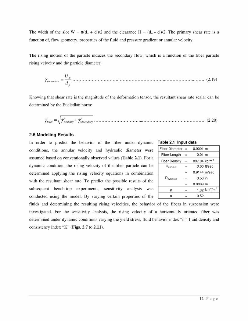
2.5 Modeling Results

In order to predict the behavior of the fiber under dynamic

conditions, the annular velocity and hydraulic diameter were

assumed based on conventionally observed values (Table 2.1). For a

dynamic condition, the rising velocity of the fiber particle can be

determined applying the rising velocity equations in combination

with the resultant shear rate. To predict the possible results of the

subsequent bench-top experiments, sensitivity analysis was

conducted using the model. By varying certain properties of the

fluids and determining the resulting rising velocities, the behavior of the fibers in suspension were

investigated. For the sensitivity analysis, the rising velocity of a horizontally oriented fiber was

determined under dynamic conditions varying the yield stress, fluid behavior index “n”, fluid density and

consistency index “K” (Figs. 2.7 to 2.11).

Table 2.1 Input data

Fiber Diameter = 0.0001 m

Fiber Length = 0.01 m

Fiber Density = 897.04 kg/m3

Uannulus = 3.00 ft/sec

= 0.9144 m/sec

Dhydraulic = 3.50 in

= 0.0889 m

K = 1.32 N-sn/m

2

n = 0.52

13 | P a g e

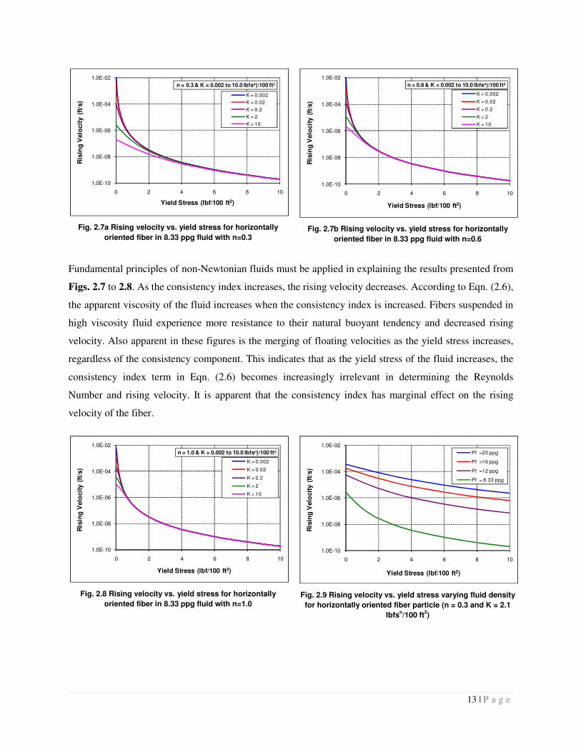
Fig. 2.7a Rising velocity vs. yield stress for horizontally

oriented fiber in 8.33 ppg fluid with n=0.3

Fig. 2.7b Rising velocity vs. yield stress for horizontally


Fundamental principles of non-Newtonian fluids must be applied in explaining the results presented from

Figs. 2.7 to 2.8. As the consistency index increases, the rising velocity decreases. According to Eqn. (2.6),

the apparent viscosity of the fluid increases when the consistency index is increased. Fibers suspended in

high viscosity fluid experience more resistance to their natural buoyant tendency and decreased rising

velocity. Also apparent in these figures is the merging of floating velocities as the yield stress increases,

regardless of the consistency component. This indicates that as the yield stress of the fluid increases, the

consistency index term in Eqn. (2.6) becomes increasingly irrelevant in determining the Reynolds

Number and rising velocity. It is apparent that the consistency index has marginal effect on the rising

velocity of the fiber.

Fig. 2.8 Rising velocity vs. yield stress for horizontally


Fig. 2.9 Rising velocity vs. yield stress varying fluid density

for horizontally oriented fiber particle (n = 0.3 and K = 2.1

lbfsn/100 ft

2)

1.0E-10

1.0E-08

1.0E-06

1.0E-04

1.0E-02

0 2 4 6 8 10

Ris

ing

Velo

cit

y (

ft/s

)

Yield Stress (lbf/100 ft2)

n = 0.3 & K = 0.002 to 10.0 lbfsn)/100 ft2

K = 0.002

K = 0.02

K = 0.2

K = 2

K = 10

1.0E-10

1.0E-08

1.0E-06

1.0E-04

1.0E-02

0 2 4 6 8 10

Ris

ing

Velo

cit

y (

ft/s

)


n = 0.6 & K = 0.002 to 10.0 lbfsn)/100 ft2

K = 0.002

K = 0.02

K = 0.2

K = 2

K = 10

1.0E-10

1.0E-08

1.0E-06

1.0E-04

1.0E-02

0 2 4 6 8 10

Ris

ing

Velo

cit

y (

ft/s

)


n = 1.0 & K = 0.002 to 10.0 lbfsn)/100 ft2

K = 0.002

K = 0.02

K = 0.2

K = 2

K = 10

1.0E-10

1.0E-08

1.0E-06

1.0E-04

1.0E-02

0 2 4 6 8 10

Ris

ing

Velo

cit

y (

ft/s

)


Pf =20 ppg

Pf =16 ppg

Pf =12 ppg

Pf = 8.33 ppg

14 | P a g e

Fig. 2.10 Rising velocity vs. yield stress varying fluid

density for horizontally oriented fiber particle (n = 0.6 and K

= 2.1 lbfsn/100 ft

2)

Fig. 2.11 Rising velocity vs. yield stress varying fluid

density for horizontally oriented fiber particle (n = 1.0 and K

= 2.1 lbfsn/100 ft

2)

The yield stress and inherent “n” value of a specific fluid characterizes the degree to which the fluid

behavior is non-Newtonian. Another trend worth investigating from Figs. 2.7 to 2.8 is the relative

closeness of the rising velocity plots for different fluids with respect to their fluid behavior indices. It is

observed that as the fluid behavior index “n” increasingly deviates from unity, the spread of the rising

velocity plots at low yield stress values tends to increase. A careful examination of Figs 2.7 and 2.8

reveals that the increase in the value of “n” substantially increases the rising velocity in fluids with high

“K” values. Even though this is unusual observation, analysis of Eqn. (2.6) shows that, at low shear rates

(i.e., shear rates less than 1 s-1), decreasing the values of “n” results in increased apparent viscosity.

To explore the effect of yield stress on the upward motion of the fiber particles further, the rising velocity

of a horizontal fiber was analyzed varying the yield stress, fluid density and flow behavior index. From

Figs. 2.9 to 2.11, it can be seen that as the density of the fluid increased, the rising velocity increased.

This was attributed to buoyancy; as the fluid became denser than the fiber, the fiber tended to ascend to

the surface faster. This also correlates to the fact that the less dense fluids require smaller yield stresses to

decrease the rising velocity or indefinitely suspend the fibers.

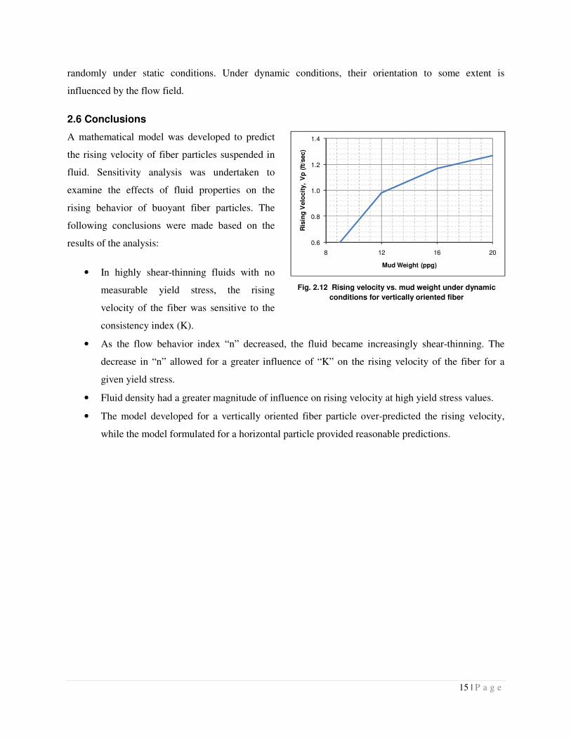
For a vertically oriented fiber particle, the rising velocity strictly relies on the fiber dimensions and

density difference between the particles and the fluid. As shown from Eqn. (2.5), when the fiber particle

orients itself in the direction of motion, the drag coefficient becomes independent of the Reynolds

Number and rheological properties of the fluid. Due to the high aspect ratio and low drag coefficient of

the fiber, the rising velocity of a vertically oriented fiber particle is very high. For a given fiber density,

the rising velocity increases with the increase in mud density (Fig. 2.12). Due to the flexibility of the fiber

and high hydraulic instability, vertical configuration is difficult to maintain; therefore, predicted values do

not reflect the actual rising speeds. In real situations, fibers are not perfectly straight. They also orient

1.0E-10

1.0E-08

1.0E-06

1.0E-04

1.0E-02

0 2 4 6 8 10

Ris

ing

Velo

cit

y (

ft/s

)


Pf =20 ppg

Pf =16 ppg

Pf =12 ppg

Pf = 8.33 ppg

1.0E-10

1.0E-08

1.0E-06

1.0E-04

1.0E-02

0 2 4 6 8 10

Ris

ing

Velo

cit

y (

ft/s

)


Pf =20 ppg

Pf =16 ppg

Pf =12 ppg

Pf = 8.33 ppg

15 | P a g e

randomly under static conditions. Under dynamic conditions, their orientation to some extent is

influenced by the flow field.

2.6 Conclusions

A mathematical model was developed to predict

the rising velocity of fiber particles suspended in

fluid. Sensitivity analysis was undertaken to

examine the effects of fluid properties on the

rising behavior of buoyant fiber particles. The

following conclusions were made based on the

results of the analysis:

• In highly shear-thinning fluids with no

measurable yield stress, the rising

velocity of the fiber was sensitive to the

consistency index (K).

• As the flow behavior index “n” decreased, the fluid became increasingly shear-thinning. The

decrease in “n” allowed for a greater influence of “K” on the rising velocity of the fiber for a

given yield stress.

• Fluid density had a greater magnitude of influence on rising velocity at high yield stress values.

• The model developed for a vertically oriented fiber particle over-predicted the rising velocity,

while the model formulated for a horizontal particle provided reasonable predictions.

Fig. 2.12 Rising velocity vs. mud weight under dynamic

conditions for vertically oriented fiber

0.6

0.8

1.0

1.2

1.4

8 12 16 20

Ris

ing

Velo

cit

y,

Vp

(ft

/sec)

Mud Weight (ppg)

16 | P a g e

Nomenclature

Ap,h = projection area of horizontally oriented

particle

Ap,v = projection area of vertically oriented particle

CD,h = Drag coefficient for a horizontally oriented

particle

CD,v = Drag coefficient for a vertically oriented

particle

d = diameter of fiber particle

di = inner diameter of annulus

do = outer diameter of annulus

Dh = hydraulic diameter (Douter – Dinner)

FB = Buoyancy force

FD = Drag force

g = gravitational acceleration

K = consistency index

L = length of the fiber

m = Mass of a fiber particle

n = flow behavior index

Re = Reynolds Number

R = particle radius (m)

Up,h = rising velocity of particle

Up,h = rising velocity of a horizontally oriented

fiber particle

Up,v = rising velocity of a vertically oriented fiber

particle

W = weight of a fiber particle

VP = volume of a fiber particle

Greek Letters �� = Shear rate

aveγ& = Average shear rate

primaryγ& = Primary shear rate

ondarysecγ& = Secondary shear rate

totalγ& = Total/overall shear rate

µ = fluid viscosity

µapp = Apparent fluid viscosity

θ = Angle

ρf = Fluid density

ρp = Density of a particle

τy = yield stress

τy,h = critical yield stress for a horizontally oriented

particle

τy,h = critical yield stress for a vertically oriented

particle

17 | P a g e

References

Ahmed, R.M. and Takach, N.E. 2008. Fiber Sweeps for Hole Cleaning. Paper SPE 113746 presented at

the Coiled Tubing and Well Intervention Conference and Exhibition, The Woodlands, Texas, 1-2

April. doi: 10.2118/113746.

Dedegil, M.Y. 1987. Drag Coefficient and Settling Velocity of Particles in Non-Newtonian Suspensions.

Journal of Fluids Engineering 109 (3): 319-323.

Fan, L, Mao, Z., and Yang, C. 2004. Experiment on Settling of Slender Particles with Large Aspect Ratio

and Correlation of the Drag Coefficient. Ind. Eng. Chem. Res. 43 (23): 7664-7670.

Herzhaft, B., Guazzelli, E., Mackaplow, M., & Shaqfeh, E. 1996. Experimental Investigation of a

Sedimentation of a Dilute Fiber Suspension. Phys. Rev. Lett. 77 (2): 290-293Hoerner, S. F.

(1965): Fluid-Dynamic Drag. Hoerner Fluid Dynamics, Brick Town, New Jersey.

Herzhaft, B. & Guazzelli, E. 1999. Experimental Study of Sedimentation of Dilute and Semi-Dilute

Suspensions of Fibres. J. Fluid Mech. 384: 133-158Metzner, A.B. and Reed, J.C. 1955. Flow of

Non-Newtonian Fluids – Correlation of the Laminar, Transition, and Turbulent-flow Regions.

A.I.Ch.E. Journal 1 (4): 434-440.

Koch, D. & Shaqfeh, E. 1989. The Instability of a Dispersion of Sedimenting Spheroids. J. Fluid Mech.

209: 521-542.

Kuusela, E., Hofler, K., & Schwarzer, S. 2001. Computation of Particle Settling Speed and Orientation

Distribution in Suspensions of Prolate Spheroids. J. Eng. Math. 41 (2-3): 221-235.

Kuusela, E. & Lahtinen, J. 2003. Collective Effects in Settling of Spheroids Under Steady-State

Sedimentation. Phys. Rev. Lett. 90 (9): 1-4.

Liu, Y.J. & Joseph, D.D. 1993. Sedimentation of Particles in Polymer Solutions. J. Fluid Mech. 255: 565-

595.

Miska, S. 2007. Advanced Drilling, Course Material, University of Tulsa.

Perry, R.H. and Green, D.W. 1984. Perry’s Chemical Engineering Handbook. 6th Edition. Japan:

McGraw-Hill.

Qi, G.Q., Nathan, G.J., & Kelso, R.M. 2011. Aerodynamics of Long Aspect Ratio Fibrous Particles

Under Settling. Paper AJTEC2011-44061 presented at the ASME/JSME 8th Thermal

Engineering Joint Conference, Honolulu, Hawaii, USA, 13-17 March.

Scholz, M. 2006. Wetland Systems to Control Urban Runoff. Amsterdam, The Netherlands: Elsevier.

18 | P a g e

3. Experimental Study on Stability of Fiber Sweeps

The current investigation involved experimental studies of the stability of the fiber in various fluids at

ambient and high temperatures. Several base fluids were chosen to simulate typical drilling and sweep

fluids utilized in the field.

3.1 Scope

The purpose of this investigation was to determine how well various base fluids hold the fiber in

suspension under ambient and high temperature conditions. The fibers had a specific gravity of

approximately 0.9, which was less dense than the typical fluids in which they are suspended. Therefore,

their natural tendency was to rise to the surface of the fluid and form fiber lumps. If the fibers rose while

suspended in the fluid, the hole cleaning performance of the fluid diminished and fiber lumps might plug

some of the downhole tools. As discussed previously, fiber sweep is mainly applied to reduce cuttings in

the wellbore. The fluids utilized for the sweep operations must possess properties conducive to

maintaining a uniform fiber concentration throughout the bulk volume without increasing the ECD.

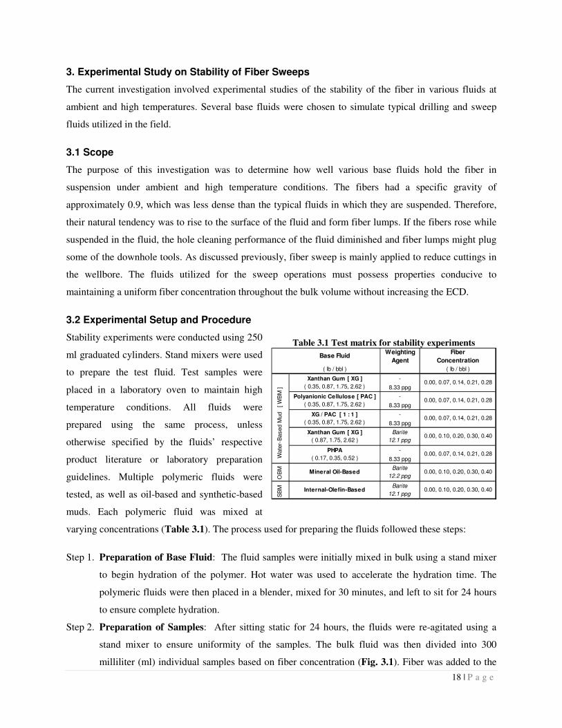
3.2 Experimental Setup and Procedure

Stability experiments were conducted using 250

ml graduated cylinders. Stand mixers were used

to prepare the test fluid. Test samples were

placed in a laboratory oven to maintain high

temperature conditions. All fluids were

prepared using the same process, unless

otherwise specified by the fluids’ respective

product literature or laboratory preparation

guidelines. Multiple polymeric fluids were

tested, as well as oil-based and synthetic-based

muds. Each polymeric fluid was mixed at

varying concentrations (Table 3.1). The process used for preparing the fluids followed these steps:

Step 1. Preparation of Base Fluid: The fluid samples were initially mixed in bulk using a stand mixer

to begin hydration of the polymer. Hot water was used to accelerate the hydration time. The

polymeric fluids were then placed in a blender, mixed for 30 minutes, and left to sit for 24 hours

to ensure complete hydration.

Step 2. Preparation of Samples: After sitting static for 24 hours, the fluids were re-agitated using a

stand mixer to ensure uniformity of the samples. The bulk fluid was then divided into 300

milliliter (ml) individual samples based on fiber concentration (Fig. 3.1). Fiber was added to the

Table 3.1 Test matrix for stability experiments Weighting Fiber

Agent Concentration

( lb / bbl ) ( lb / bbl )

Xanthan Gum [ XG ] -

( 0.35, 0.87, 1.75, 2.62 ) 8.33 ppg

Polyanionic Cellulose [ PAC ] -

( 0.35, 0.87, 1.75, 2.62 ) 8.33 ppg

XG / PAC [ 1 : 1 ] -

( 0.35, 0.87, 1.75, 2.62 ) 8.33 ppg

Xanthan Gum [ XG ] Barite

( 0.87, 1.75, 2.62 ) 12.1 ppg

PHPA -

( 0.17, 0.35, 0.52 ) 8.33 ppg

Barite

12.2 ppg

Barite

12.1 ppg

OB

M

Mineral Oil-Based 0.00, 0.10, 0.20, 0.30, 0.40

SB

M Internal-Olefin-Based 0.00, 0.10, 0.20, 0.30, 0.40

Base Fluid

W

ate

r-B

ased M

ud [ W

BM

]

0.00, 0.07, 0.14, 0.21, 0.28

0.00, 0.07, 0.14, 0.21, 0.28

0.00, 0.07, 0.14, 0.21, 0.28

0.00, 0.10, 0.20, 0.30, 0.40

0.00, 0.07, 0.14, 0.21, 0.28

19 | P a g e

samples by volumetric concentration in increments of 0.07, 0.14, 0.21, and 0.28 lb/bbl for

unweighted, water-based fluid (approx. 0.02, 0.04, 0.06, and 0.08 percent by weight for 8.33

lb/gal mud).

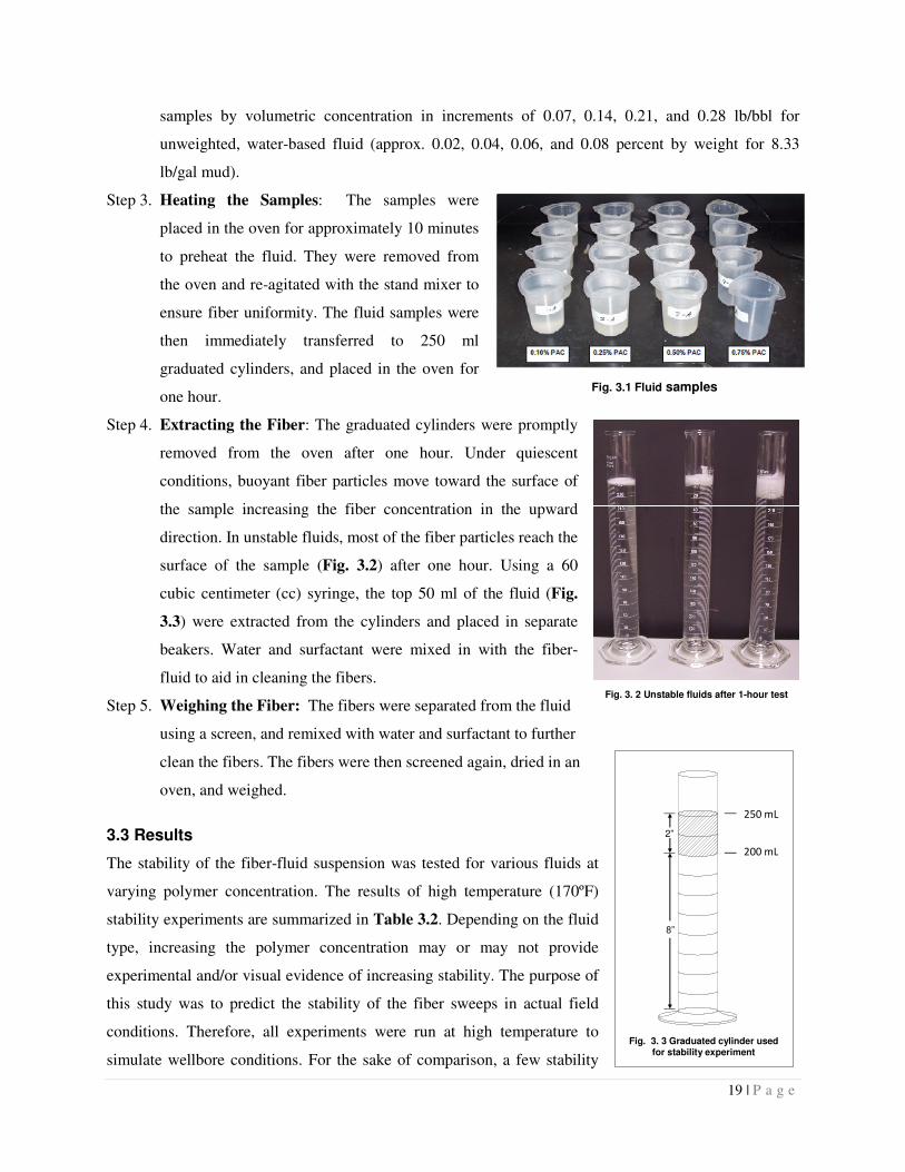
Step 3. Heating the Samples: The samples were

placed in the oven for approximately 10 minutes

to preheat the fluid. They were removed from

the oven and re-agitated with the stand mixer to

ensure fiber uniformity. The fluid samples were

then immediately transferred to 250 ml

graduated cylinders, and placed in the oven for

one hour.

Step 4. Extracting the Fiber: The graduated cylinders were promptly

removed from the oven after one hour. Under quiescent

conditions, buoyant fiber particles move toward the surface of

the sample increasing the fiber concentration in the upward

direction. In unstable fluids, most of the fiber particles reach the

surface of the sample (Fig. 3.2) after one hour. Using a 60

cubic centimeter (cc) syringe, the top 50 ml of the fluid (Fig.

3.3) were extracted from the cylinders and placed in separate

beakers. Water and surfactant were mixed in with the fiber-

fluid to aid in cleaning the fibers.

Step 5. Weighing the Fiber: The fibers were separated from the fluid

using a screen, and remixed with water and surfactant to further

clean the fibers. The fibers were then screened again, dried in an

oven, and weighed.

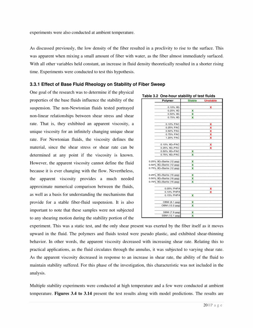
3.3 Results

The stability of the fiber-fluid suspension was tested for various fluids at

varying polymer concentration. The results of high temperature (170ºF)

stability experiments are summarized in Table 3.2. Depending on the fluid

type, increasing the polymer concentration may or may not provide

experimental and/or visual evidence of increasing stability. The purpose of

this study was to predict the stability of the fiber sweeps in actual field

conditions. Therefore, all experiments were run at high temperature to

simulate wellbore conditions. For the sake of comparison, a few stability

Fig. 3. 2 Unstable fluids after 1-hour test

Fig. 3. 3 Graduated cylinder used for stability experiment

250 mL

200 mL

2”

8”

Fig. 3.1 Fluid samples

20 | P a g e

experiments were also conducted at ambient temperature.

As discussed previously, the low density of the fiber resulted in a proclivity to rise to the surface. This

was apparent when mixing a small amount of fiber with water, as the fiber almost immediately surfaced.

With all other variables held constant, an increase in fluid density theoretically resulted in a shorter rising

time. Experiments were conducted to test this hypothesis.

3.3.1 Effect of Base Fluid Rheology on Stability of Fiber Sweep

One goal of the research was to determine if the physical

properties of the base fluids influence the stability of the

suspension. The non-Newtonian fluids tested portrayed

non-linear relationships between shear stress and shear

rate. That is, they exhibited an apparent viscosity, a

unique viscosity for an infinitely changing unique shear

rate. For Newtonian fluids, the viscosity defines the

material, since the shear stress or shear rate can be

determined at any point if the viscosity is known.

However, the apparent viscosity cannot define the fluid

because it is ever changing with the flow. Nevertheless,

the apparent viscosity provides a much needed

approximate numerical comparison between the fluids,

as well as a basis for understanding the mechanisms that

provide for a stable fiber-fluid suspension. It is also

important to note that these samples were not subjected

to any shearing motion during the stability portion of the

experiment. This was a static test, and the only shear present was exerted by the fiber itself as it moves

upward in the fluid. The polymers and fluids tested were pseudo plastic, and exhibited shear-thinning

behavior. In other words, the apparent viscosity decreased with increasing shear rate. Relating this to

practical applications, as the fluid circulates through the annulus, it was subjected to varying shear rate.

As the apparent viscosity decreased in response to an increase in shear rate, the ability of the fluid to

maintain stability suffered. For this phase of the investigation, this characteristic was not included in the

analysis.

Multiple stability experiments were conducted at high temperature and a few were conducted at ambient

temperature. Figures 3.4 to 3.14 present the test results along with model predictions. The results are

Table 3.2 One-hour stability of test fluids

Stable Unstable

0.10% XG X

0.25% XG X

0.50% XG X

0.75% XG X

0.10% PAC X

0.25% PAC X

0.50% PAC X

0.75% PAC X

1.20% PAC X

0.10% XG+PAC X

0.25% XG+PAC X

0.50% XG+PAC X

0.75% XG+PAC X

0.25% XG+Barite (12 ppg) X






0.05% PHPA X

0.10% PHPA X

0.15% PHPA X

OBM (8.1 ppg) X

OBM (12.2 ppg) X

SBM (7.9 ppg) X

SBM (12.1 ppg) X

Polymer

21 | P a g e

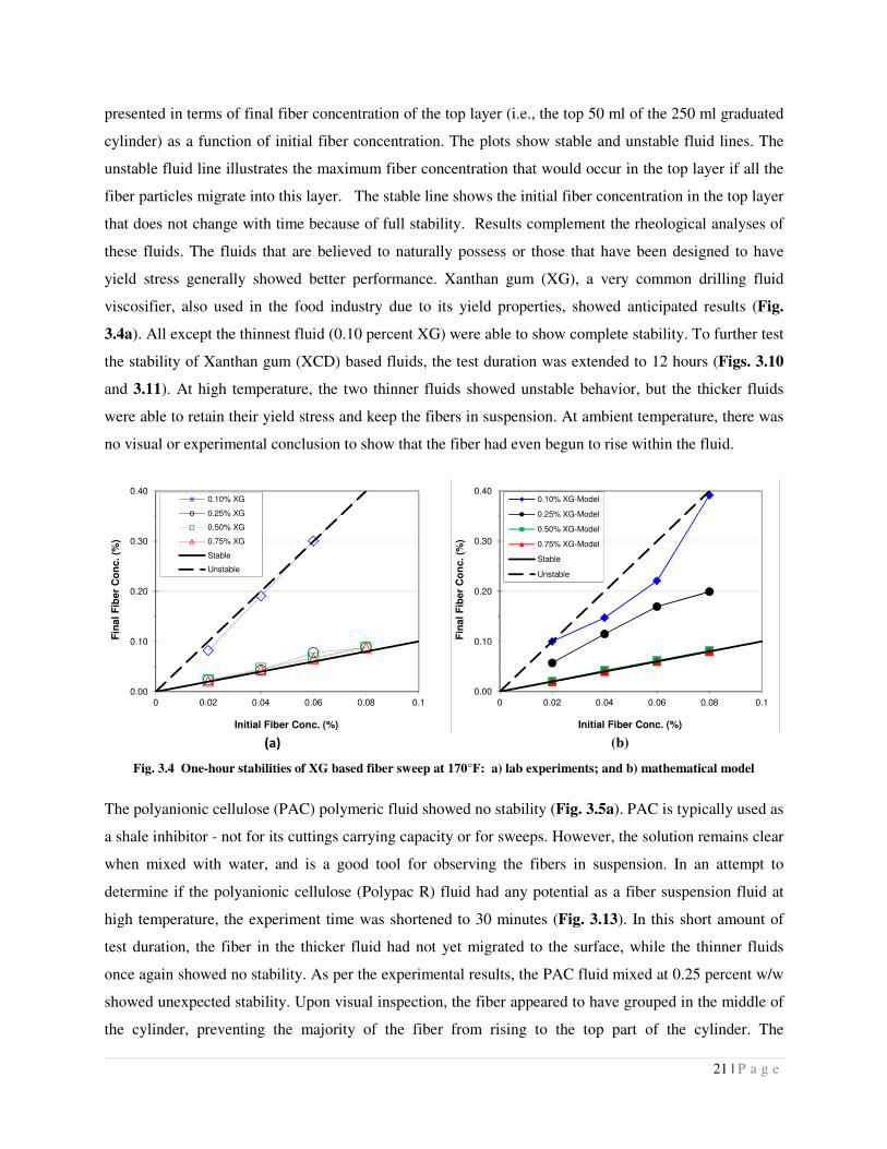
presented in terms of final fiber concentration of the top layer (i.e., the top 50 ml of the 250 ml graduated

cylinder) as a function of initial fiber concentration. The plots show stable and unstable fluid lines. The

unstable fluid line illustrates the maximum fiber concentration that would occur in the top layer if all the

fiber particles migrate into this layer. The stable line shows the initial fiber concentration in the top layer

that does not change with time because of full stability. Results complement the rheological analyses of

these fluids. The fluids that are believed to naturally possess or those that have been designed to have

yield stress generally showed better performance. Xanthan gum (XG), a very common drilling fluid

viscosifier, also used in the food industry due to its yield properties, showed anticipated results (Fig.

3.4a). All except the thinnest fluid (0.10 percent XG) were able to show complete stability. To further test

the stability of Xanthan gum (XCD) based fluids, the test duration was extended to 12 hours (Figs. 3.10

and 3.11). At high temperature, the two thinner fluids showed unstable behavior, but the thicker fluids

were able to retain their yield stress and keep the fibers in suspension. At ambient temperature, there was

no visual or experimental conclusion to show that the fiber had even begun to rise within the fluid.

(a) (b)

Fig. 3.4 One-hour stabilities of XG based fiber sweep at 170°F: a) lab experiments; and b) mathematical model

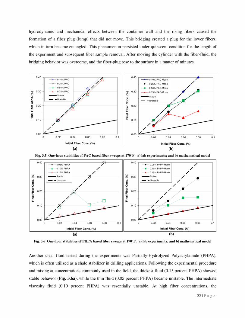
The polyanionic cellulose (PAC) polymeric fluid showed no stability (Fig. 3.5a). PAC is typically used as

a shale inhibitor - not for its cuttings carrying capacity or for sweeps. However, the solution remains clear

when mixed with water, and is a good tool for observing the fibers in suspension. In an attempt to

determine if the polyanionic cellulose (Polypac R) fluid had any potential as a fiber suspension fluid at

high temperature, the experiment time was shortened to 30 minutes (Fig. 3.13). In this short amount of

test duration, the fiber in the thicker fluid had not yet migrated to the surface, while the thinner fluids

once again showed no stability. As per the experimental results, the PAC fluid mixed at 0.25 percent w/w

showed unexpected stability. Upon visual inspection, the fiber appeared to have grouped in the middle of

the cylinder, preventing the majority of the fiber from rising to the top part of the cylinder. The

0.00

0.10

0.20

0.30

0.40

0 0.02 0.04 0.06 0.08 0.1

Fin

al

Fib

er

Co

nc. (%

)

Initial Fiber Conc. (%)

0.10% XG

0.25% XG

0.50% XG

0.75% XG

Stable

Unstable

0.00

0.10

0.20

0.30

0.40

0 0.02 0.04 0.06 0.08 0.1

Fin

al

Fib

er

Co

nc. (%

)


0.10% XG-Model

0.25% XG-Model

0.50% XG-Model

0.75% XG-Model

Stable

Unstable

22 | P a g e

hydrodynamic and mechanical effects between the container wall and the rising fibers caused the

formation of a fiber plug (lump) that did not move. This bridging created a plug for the lower fibers,

which in turn became entangled. This phenomenon persisted under quiescent condition for the length of

the experiment and subsequent fiber sample removal. After moving the cylinder with the fiber-fluid, the

bridging behavior was overcome, and the fiber-plug rose to the surface in a matter of minutes.

(a) (b)

Fig. 3.5 One-hour stabilities of PAC based fiber sweeps at 170°F: a) lab experiments; and b) mathematical model

(a) (b)

Fig. 3.6 One-hour stabilities of PHPA based fiber sweeps at 170°F: a) lab experiments; and b) mathematical model

Another clear fluid tested during the experiments was Partially-Hydrolyzed Polyacrylamide (PHPA),

which is often utilized as a shale stabilizer in drilling applications. Following the experimental procedure

and mixing at concentrations commonly used in the field, the thickest fluid (0.15 percent PHPA) showed

stable behavior (Fig. 3.6a), while the thin fluid (0.05 percent PHPA) became unstable. The intermediate

viscosity fluid (0.10 percent PHPA) was essentially unstable. At high fiber concentrations, the

0.00

0.10

0.20

0.30

0.40

0 0.02 0.04 0.06 0.08 0.1

Fin

al

Fib

er

Co

nc

. (%

)


0.10% PAC

0.25% PAC

0.50% PAC

0.75% PAC

Stable

Unstable

0.00

0.10

0.20

0.30

0.40

0 0.02 0.04 0.06 0.08 0.1

Fin

al

Fib

er

Co

nc

. (%

)


0.05% PHPA

0.10% PHPA

0.15% PHPA

Stable

Unstable

0.00

0.10

0.20

0.30

0.40

0 0.02 0.04 0.06 0.08 0.1

Fin

al

Fib

er

Co

nc. (%

)


0.10% PAC-Model

0.25% PAC-Model

0.50% PAC-Model

0.75% PAC-Model

Stable

Unstable

0.00

0.10

0.20

0.30

0.40

0 0.02 0.04 0.06 0.08 0.1

Fin

al

Fib

er

Co

nc

. (%

)


0.05% PHPA-Model

0.10% PHPA-Model

0.15% PHPA-Model

Stable

Unstable

23 | P a g e

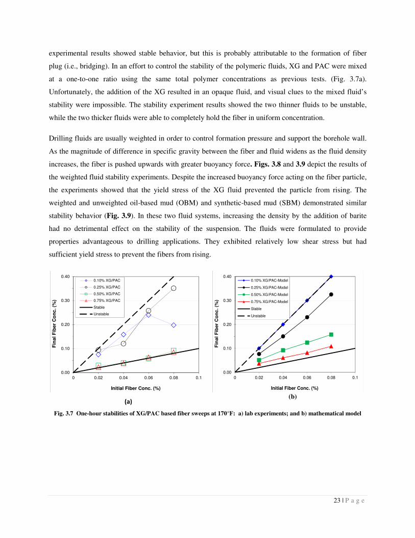
experimental results showed stable behavior, but this is probably attributable to the formation of fiber

plug (i.e., bridging). In an effort to control the stability of the polymeric fluids, XG and PAC were mixed

at a one-to-one ratio using the same total polymer concentrations as previous tests. (Fig. 3.7a).

Unfortunately, the addition of the XG resulted in an opaque fluid, and visual clues to the mixed fluid’s

stability were impossible. The stability experiment results showed the two thinner fluids to be unstable,

while the two thicker fluids were able to completely hold the fiber in uniform concentration.

Drilling fluids are usually weighted in order to control formation pressure and support the borehole wall.

As the magnitude of difference in specific gravity between the fiber and fluid widens as the fluid density

increases, the fiber is pushed upwards with greater buoyancy force. Figs. 3.8 and 3.9 depict the results of

the weighted fluid stability experiments. Despite the increased buoyancy force acting on the fiber particle,

the experiments showed that the yield stress of the XG fluid prevented the particle from rising. The

weighted and unweighted oil-based mud (OBM) and synthetic-based mud (SBM) demonstrated similar

stability behavior (Fig. 3.9). In these two fluid systems, increasing the density by the addition of barite

had no detrimental effect on the stability of the suspension. The fluids were formulated to provide

properties advantageous to drilling applications. They exhibited relatively low shear stress but had

sufficient yield stress to prevent the fibers from rising.

(a) (b)

Fig. 3.7 One-hour stabilities of XG/PAC based fiber sweeps at 170°F: a) lab experiments; and b) mathematical model

0.00

0.10

0.20

0.30

0.40

0 0.02 0.04 0.06 0.08 0.1

Fin

al F

iber

Co

nc. (%

)


0.10% XG/PAC

0.25% XG/PAC

0.50% XG/PAC

0.75% XG/PAC

Stable

Unstable

0.00

0.10

0.20

0.30

0.40

0 0.02 0.04 0.06 0.08 0.1

Fin

al

Fib

er

Co

nc

. (%

)


0.10% XG/PAC-Model

0.25% XG/PAC-Model

0.50% XG/PAC-Model

0.75% XG/PAC-Model

Stable

Unstable

24 | P a g e

(a) (b)

Fig. 3.8 One-hour stabilities of XG based weighted (12 ppg) fiber sweeps at 170°F:

a) lab experiments; and b) mathematical model

(a) (b)

Fig. 3.9 Measured and predicted one-hour stability of oil-based fluids at 170°F: a) OBM; and b) SBM

Fig. 3.10 Twelve-hour stabilities of XG based fluids at 170°F

Fig. 3.11 Twelve-hour stabilities of XG based fluids at 72°F

0.00

0.10

0.20

0.30

0.40

0 0.02 0.04 0.06 0.08 0.1

Fin

al F

iber

Co

nc.

(%)


0.25% XG-Model

0.50% XG-Model

0.75% XG-Model

Stable

Unstable

0.00

0.10

0.20

0.30

0.40

0 0.02 0.04 0.06 0.08 0.1

Fin

al

Fib

er

Co

nc

. (%

)


8.1 ppg

8.1 ppg-Model

12.2 ppg

12.2 ppg-Model

Stable

Unstable

0.00

0.10

0.20

0.30

0.40

0 0.02 0.04 0.06 0.08 0.1

Fin

al F

iber

Co

nc.

(%)


0.10% XG

0.25% XG

0.50% XG

0.75% XG

Stable

Unstable

0.00

0.10

0.20

0.30

0.40

0 0.02 0.04 0.06 0.08 0.1

Fin

al F

iber

Co

nc.

(%)


0.10% XG

0.25% XG

0.50% XG

0.75% XG

Stable

Unstable

0.00

0.10

0.20

0.30

0.40

0 0.02 0.04 0.06 0.08 0.1

Fin

al

Fib

er

Co

nc

. (%

)


7.9 ppg

7.9 ppg-Model

12.1 ppg

12.1 ppg-Model

Stable

Unstable

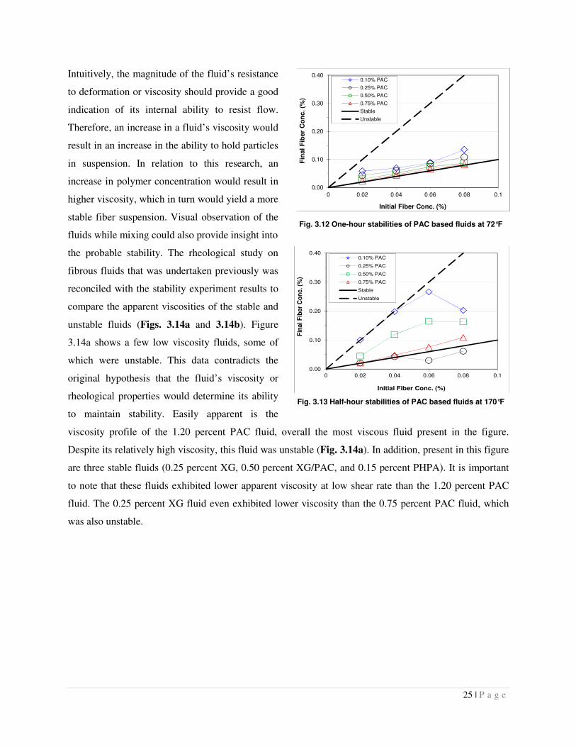
25 | P a g e

Intuitively, the magnitude of the fluid’s resistance

to deformation or viscosity should provide a good

indication of its internal ability to resist flow.

Therefore, an increase in a fluid’s viscosity would

result in an increase in the ability to hold particles

in suspension. In relation to this research, an

increase in polymer concentration would result in

higher viscosity, which in turn would yield a more

stable fiber suspension. Visual observation of the

fluids while mixing could also provide insight into

the probable stability. The rheological study on

fibrous fluids that was undertaken previously was

reconciled with the stability experiment results to

compare the apparent viscosities of the stable and

unstable fluids (Figs. 3.14a and 3.14b). Figure

3.14a shows a few low viscosity fluids, some of

which were unstable. This data contradicts the

original hypothesis that the fluid’s viscosity or

rheological properties would determine its ability

to maintain stability. Easily apparent is the

viscosity profile of the 1.20 percent PAC fluid, overall the most viscous fluid present in the figure.

Despite its relatively high viscosity, this fluid was unstable (Fig. 3.14a). In addition, present in this figure

are three stable fluids (0.25 percent XG, 0.50 percent XG/PAC, and 0.15 percent PHPA). It is important

to note that these fluids exhibited lower apparent viscosity at low shear rate than the 1.20 percent PAC

fluid. The 0.25 percent XG fluid even exhibited lower viscosity than the 0.75 percent PAC fluid, which

was also unstable.

Fig. 3.12 One-hour stabilities of PAC based fluids at 72°F

Fig. 3.13 Half-hour stabilities of PAC based fluids at 170°F

0.00

0.10

0.20

0.30

0.40

0 0.02 0.04 0.06 0.08 0.1

Fin

al F

iber

Co

nc. (%

)


0.10% PAC

0.25% PAC

0.50% PAC

0.75% PAC

Stable

Unstable

0.00

0.10

0.20

0.30

0.40

0 0.02 0.04 0.06 0.08 0.1

Fin

al

Fib

er

Co

nc. (%

)


0.10% PAC

0.25% PAC

0.50% PAC

0.75% PAC

Stable

Unstable

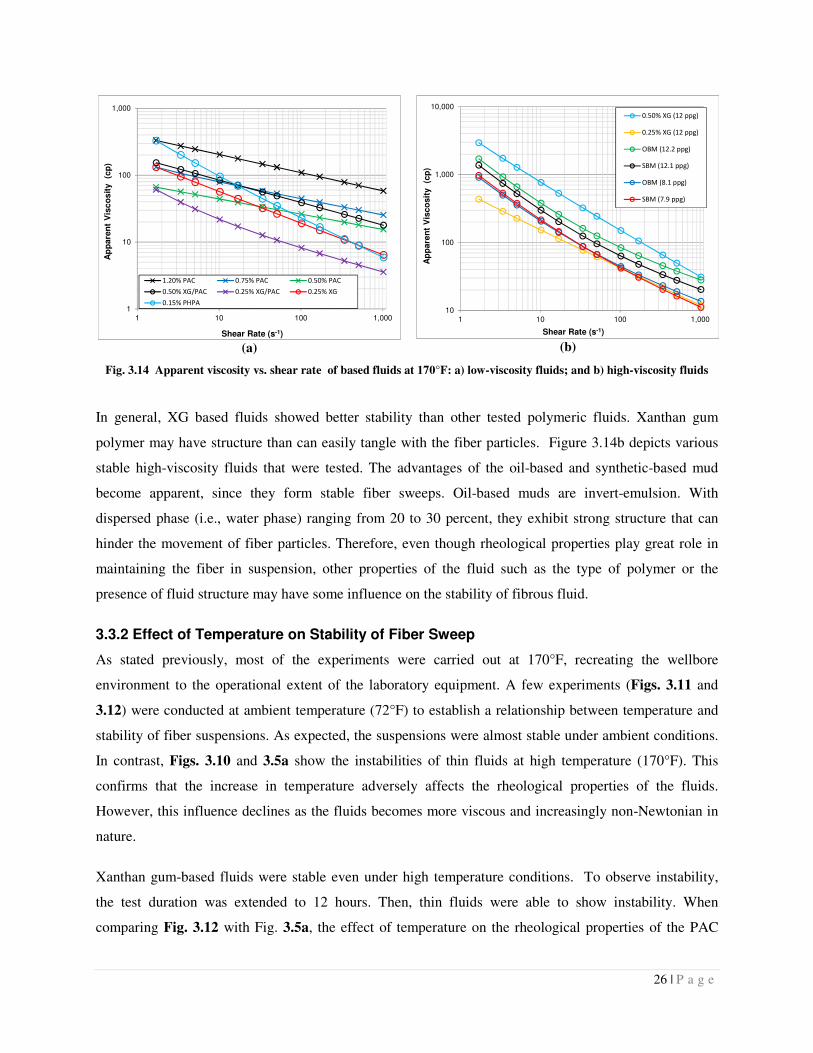
26 | P a g e

(a) (b)

Fig. 3.14 Apparent viscosity vs. shear rate of based fluids at 170°F: a) low-viscosity fluids; and b) high-viscosity fluids

In general, XG based fluids showed better stability than other tested polymeric fluids. Xanthan gum

polymer may have structure than can easily tangle with the fiber particles. Figure 3.14b depicts various

stable high-viscosity fluids that were tested. The advantages of the oil-based and synthetic-based mud

become apparent, since they form stable fiber sweeps. Oil-based muds are invert-emulsion. With

dispersed phase (i.e., water phase) ranging from 20 to 30 percent, they exhibit strong structure that can

hinder the movement of fiber particles. Therefore, even though rheological properties play great role in

maintaining the fiber in suspension, other properties of the fluid such as the type of polymer or the

presence of fluid structure may have some influence on the stability of fibrous fluid.

3.3.2 Effect of Temperature on Stability of Fiber Sweep

As stated previously, most of the experiments were carried out at 170°F, recreating the wellbore

environment to the operational extent of the laboratory equipment. A few experiments (Figs. 3.11 and

3.12) were conducted at ambient temperature (72°F) to establish a relationship between temperature and

stability of fiber suspensions. As expected, the suspensions were almost stable under ambient conditions.

In contrast, Figs. 3.10 and 3.5a show the instabilities of thin fluids at high temperature (170°F). This

confirms that the increase in temperature adversely affects the rheological properties of the fluids.

However, this influence declines as the fluids becomes more viscous and increasingly non-Newtonian in

nature.

Xanthan gum-based fluids were stable even under high temperature conditions. To observe instability,

the test duration was extended to 12 hours. Then, thin fluids were able to show instability. When

comparing Fig. 3.12 with Fig. 3.5a, the effect of temperature on the rheological properties of the PAC

1

10

100

1,000

1 10 100 1,000

Ap

pare

nt

Vis

co

sit

y

(cp

)

Shear Rate (s-1)

1.20% PAC 0.75% PAC 0.50% PAC

0.50% XG/PAC 0.25% XG/PAC 0.25% XG

0.15% PHPA10

100

1,000

10,000

1 10 100 1,000

Ap

pare

nt

Vis

co

sit

y

(cp

)

Shear Rate (s-1)

0.50% XG (12 ppg)

0.25% XG (12 ppg)

OBM (12.2 ppg)

SBM (12.1 ppg)

OBM (8.1 ppg)

SBM (7.9 ppg)

27 | P a g e

fluid becomes apparent. While the ambient temperature experiments were able to show favorable results,

increasing the temperature had adverse effects.

3.3.3 Comparison of Model Predictions with Experimental Results

The rising velocity model presented in Section 2 was developed to predict the stability of the fiber

suspension or determine fluid properties necessary to prevent the separation of fiber particles. These

models took into account various forces acting on each individual particle while suspended in the fluid,

such as the buoyancy force created by the difference between fiber and fluid density, and the gravitational

forced exerted on the fiber particle. The model was formulated to predict rising velocities for particles

oriented horizontal and vertical. This was done to simulate the two extreme cases of particle motion

within the fluid. The rheological parameters of the fluids obtained from viscometeric measurements were

inputs into both models to compare model predictions with the actual experimental measurements. As the

tested fluids exhibit non-Newtonian behavior, the rising velocity of the fiber particles becomes a function

of rheological parameters of the fluid. The Yield Power Law (YPL) model is the most accurate

constitutive equation to describe the majority of drilling fluids currently used in the industry. From the

rheological measurements, the parameters of the test fluids were determined using regression analysis and

used in the models. By determining the distance the fiber particles rose in one hour and the amount of

fiber that entered into the top layer in that period, we were able to estimate the final concentrations of the

top layer. Model predictions shown from Figs. 3.4 to 3.9 were obtained using the horizontal orientation

model. These results compared favorably with the test results. Predominately, the predictions were

consistent with the measurements. However, in some cases, discrepancies were substantial. For instance,

PAC based fluids did not show the ability to hold the fiber in suspension, but the model predictions for

highly viscous fluid (0.75 percent PAC) showed some form of intermediate stability at high fiber

concentrations.

The predictions of the vertical orientation model were also compared with measurements, but the results

were very dissimilar. The model predicted all fluids to be unstable. This contradicted the experimental

results, which demonstrated many of the fluids tested to be stable. When comparing the two mathematical

models, the dimensional terms differed. For both models, the area projected to the fluid flow depended on

the orientation of the fiber. If the fiber was oriented perpendicularly, the rectangular profile variables

(length x diameter = 1.0×10-6 m2) were the governing dimensions, and the vertical orientation profile was

the circular end area (¼πd2 = 7.85×10-9 m2). However, this only partially explained the difference. The

drag coefficient (CD) was also present in both equations and was inversely proportional to rising velocity

because it counteracts the buoyancy force.

28 | P a g e

For a vertically oriented particle, drag force resisting the rising fiber is exclusively related to the fiber

aspect ratio (Hoerner 1965) and independent of the fluid properties. Conversely, for a horizontally

oriented particle, the drag force is implicitly related to the Reynolds Number (Perry 1984). The rather

large aspect ratio in comparison to the rectangular projected area and fluid property dependency resulted

in a vertically oriented particle rising velocity anywhere from three to five orders of magnitude greater

than that for horizontally oriented particles.

Fluid density is one of the controllable model parameters that has a marked influence on the stability fiber

sweep. The equation used to determine the rising velocity is a function of the difference between fluid

density and particle density. Mathematically, the rising velocity increases as the difference between the

two densities increases. In theory, an increasingly dense fluid results in a fiber moving upward

instantaneously to the surface. However, the increased viscosity associated with weighted fluid hinders

the barite particles that tend to settle in the fluid under static conditions. For instance, the model

prediction for the stability of the weighted XG based fluids (Fig. 3.8b) shows both favorable and

unfavorable results, while the experimental results indicated stable fluids with a slight departure from

complete uniformity for the two thicker fluids. With its current formulation, the model considers a single

particle rising in the fluid. It does not account for the hindering effect of barite particles. This model will

be improved in the next phase of the project.

The oil-based and synthetic-based muds showed (Fig. 3.9) remarkable stability, both experimentally and

mathematically. After performing the rheological and regression analyses, the weighted and unweighted

fluids for both muds exhibited higher yield stress. All fiber-fluid combinations tested showed stable

behavior. This was reinforced with the mathematical model predictions of similar results.

3.4 Conclusions

This study was undertaken to investigate the stability of fiber sweeps at ambient and high temperature

conditions. Experiments were conducted using different base fluids (water-based and oil-based fluids)

with varying fiber concentrations. Fibers were extracted from the samples after the test and weighed to

determine the final fiber concentration in the top layer. This data was used to determine if the fiber rose

while in the fluid sample, or if uniformity persisted throughout the length of the experiment. These

measurements were compared with stability predictions obtained from the mathematical model. After

analyzing and comparing all the data to date, the following inferences were made:

• Horizontally oriented particle model predictions were in general concurrence with the

experimental data, and reasonable real-time application performance could be predicted using the

29 | P a g e

model. The vertically oriented particle model overestimated rising velocity of fibers in all fluids

tested which did not reflect experimental results, and would not provide accurate predictions.

• Despite the dominant effect of fluid rheology on the stability of fiber sweeps, other properties of

the fluid, such as the type of polymer, the presence of fluid structure, or hindering effect of other

particles, considerably influenced stability.

• Selecting the type of polymer used for drilling sweep applications was critical in designing fluids

that stable under downhole conditions.

• Oil-based and synthetic-based fluids had high fiber stability. This could be attributed to the high

yield stress that they exhibited and the presence of emulsion structure in the two-phase system.

Nomenclature

Up = Particle floating velocity (m/sec)

d = Particle diameter (m)

Dh = Hydraulic diameter (Douter – Dinner)

ECD = Equivalent circulating density

K = Consistency index

n = Fluid behavior index

OBM = Oil-based mud

PAC = Polyanionic cellulose

PHPA = Partially Hydrolyzed Polyacrylamide

SBM = Synthetic-based mud

XG = Xanthan Gum

Greek Letters

µapp = apparent viscosity

τy = yield stress

References

Hoerner, S. F. (1965): Fluid-Dynamic Drag. Hoerner Fluid Dynamics, Brick Town, New Jersey.

Perry, R.H. and Green, D.W. 1984. Perry’s Chemical Engineering Handbook. 6th Edition. Japan:

McGraw-Hill.

30 | P a g e

4. Rheological Properties of Fiber Sweeps

Fiber-containing sweeps (fiber sweeps) are effective tools for wellbore cleaning in horizontal wells. It

has been shown that adding fiber to traditional sweeps can result in an increase in cuttings removal and

reduction in cuttings bed thickness, which reduces the amount of torque and drag in horizontal wells.

Despite some reported successes in the field and favorable research results, the fluid and fiber properties

that define and influence fiber sweep rheology are not fully understood.

The hole-cleaning capabilities of weighted sweeps, high and low viscosity sweeps, and tandem sweeps

are well documented. However, these conventional sweep methods often result in an increase in

equivalent circulating density (ECD). Fiber-containing sweeps, which have promise to overcome this

ECD disadvantage, are becoming popular alternatives. However, little detail is known about the flow and

cuttings-carrying properties of these slurries.

This article presents the rheological measurements carried out on fiber-containing sweep fluids. Tests

were conducted using various unweighted and weighted water-based, mineral oil-based and internal

olefin-based drilling fluids with concentrations of a monofilament synthetic fiber ranging up to 0.4 lb/bbl.

The rheology was measured at ambient and 170ºF. The study shows that fiber concentration has minimal

effect on viscosity, indicating a negligible increase in ECD while providing improved sweep efficiency.

These results can be useful for formulating sweep fluids utilized in deepwater applications.

4.1 Introduction

Poor hole cleaning can lead to an increase in non-productive time and costly drilling problems such as

stuck pipe, premature bit wear, slow rate of penetration, formation fracturing, and high torque and drag

(Ahmed and Takach 2008). A number of field-tested techniques have been introduced over the years to

improve hole cleaning, cuttings transport, and prevent the formation of cuttings beds in the wellbore.

Previous studies indicate that cuttings transport in directional wells is dependent on fluid rheology,

wellbore inclination angle, rotary speed of the drillpipe, flow rate, wellbore geometry, and other drilling

parameters (Valluri et al. 2006). Considering these factors, the most economical and easily employed

procedures involve adding viscosifiers and weighting agents to the drilling fluid to increase the ability of

the fluid to transport cuttings to the surface. In addition, increasing the flow rate has the ability to re-

suspend cuttings, with the maximum pump rate generally provided the best hole cleaning conditions.

However, pressure losses and the equivalent circulating density (ECD) must be considered when

increasing the flow rate. Experience shows that optimal hole cleaning occurs with turbulent flow, but

turbulent flow can erode the filter cake and borewall, as well as increase ECD. Therefore, using laminar

flow at maximum flow rate, paired with fiber sweeps and mechanical agitation such as drillstring rotation

31 | P a g e

and reciprocation, is usually the preferred method for removing cuttings beds (Cameron et al. 2003).

However, these methods often only slow the formation and buildup of cuttings beds and are not very

effective at removing cuttings beds. In response to these problems, drilling fluid sweeps are utilized. The

sweeps remove cuttings that cannot be transported to the surface during normal fluid circulation while

drilling and provide additional vertical lift to the cuttings. Sweeps can be performed in all well

inclinations from vertical to horizontal, as required by wellbore conditions. In deviated, highly inclined,

and extended reach drilling (ERD) wells, sweeps are an essential tool to facilitate wellbore cleaning.

In highly deviated wellbores and especially ERD wells, the cuttings transport performance of a drilling

fluid generally diminishes. Some highly shear-thinning fluids, such as are used in milling operations, are

an exception; even in horizontal wells, the strong viscous coupling between the rotating drill string and

fluid can bring up even metal shavings and fist-sized rock. In highly deviated wellbores, the fluid velocity

has little vertical component, reducing the ability of the drilling fluid to suspend and carry the cuttings.

The increased wellbore length results in higher ECD that limits the flow rate and provides more

opportunity for the cuttings to form a bed on the low side of the wellbore. In addition, the drillpipe rests

on the low side of the wellbore in horizontal sections, forcing the majority of the fluid to the high side and

further encouraging the formation of cuttings beds. Inadequate hole cleaning is common with ERD wells.

Sweeps containing traditional fibrous lost circulation materials (LCM) have been shown to decrease

cuttings and silt beds, as well as reduce torque and drag and improve the rate of penetration (Cameron et

al. 2003). These materials generally refer to organic fibers or plant-derived abrasive substances.

Experimental studies (Ahmed and Takach 2008) and field applications (Bulgachev and Pouget 2006)

have shown that specially designed sweeps containing synthetic monofilament fibers show improved hole

cleaning efficiency over comparable non-fiber sweeps. While these and other cases demonstrate favorable

results when utilizing fiber sweeps, the method for designing these sweeps is still not fully developed.

Visually observing shaker screens to determine whether cuttings transport rate is constant or changing and

plotting these trends versus the sweep volume and fiber concentration are the predominant methods of

monitoring hole-cleaning efficiency.

When fully dispersed in the sweep fluid, fibers form a stable network structure that tends to support

cuttings due to fiber-fiber and fiber-fluid interactions. The fiber-fiber interactions can be by direct

mechanical contact and/or hydrodynamic interference among fiber particles. Mechanical contact among

fibers improves the solids-carrying capacity of the fluid (Ahmed and Takach 2008). Mechanical contact

between the fibers and cuttings beds aid in re-suspending cuttings deposited on the low-side of the

wellbore. As the fibers flow through the annulus, mechanical stresses develop between the settled cuttings

32 | P a g e

and the fibers. These mechanical stresses result in a frictional force that helps to re-suspend the cuttings

while the fiber networks carry the solids to the surface. Also aiding in the solids transport is the fiber-fiber

interaction that enables the fiber network to move as a single phase This fiber network can separate from

the fluid phase. Therefore, at the surface of the cuttings bed the fiber may have a higher velocity than the

fluid phase, which is typically very low. These fast moving fibers can therefore transfer more momentum

to the deposited solids, overcoming the static frictional forces and initiating movement.

This study was undertaken to determine the effect of a fiber on drilling fluid rheology. This

monofilament synthetic material is used in hole-cleaning sweeps throughout the industry. Tests were

conducted of various unweighted and weighted water-based, mineral oil-based and internal olefin-based

drilling fluids with a range of fiber concentrations. The rheology was measured at ambient and 170°F.

The results are expected to be useful for formulating sweep fluids in deviated and deepwater applications.

4.2 Literature Review

Hole-cleaning sweeps may be classified as high-viscosity; high-density; low-viscosity; combinations; and

tandem (Hemphill and Rojas 2002). Factors that govern sweep selection include hole angle, fluid density,

lithology, cuttings diameter, drill pipe rotation, and fracture gradient (Power et al. 2000). In deepwater

and deviated wells, the drilling window between the fracture gradient and pore pressure generally narrows

with increasing depth and hole angle, respectively, reducing the available options for hole cleaning

sweeps. In addition, long horizontal departures are common in order to reduce the environmental impact.

This, combined with the marginal operating window, necessitates a strict adherence to a manageable

ECD. To manage the ECD properly, drilling fluid rheology must be optimized for the conditions, and the

wellbore must be as free of cuttings as possible.

Surface torque and the ability of the rig to overcome it is an important factor when deciding the feasibility

of drilling a well, especially an extended read drilling (ERD) well. The friction generated between the

wellbore and the drillstring in long horizontal sections creates the surface torque. Hole tortuosity in ERD

wells further reduces the ability of the drilling fluid to adequately carry cuttings to the surface. Leaving

cuttings behind adds resistance to the drillstring, which proportionately increases wellbore friction and

surface torque (Maehs et al. 2010). The incorporation of fibrous lost circulation material (LCM) in the

drilling fluid proved a major factor in reducing torque 25 percent on ultra-extended reach wells (Cameron

2001). In drilling an extended reach well in Abu Dhabi, the incorporation of fibrous hole cleaning sweeps

resulted in a dramatic decrease in torque and drag and increased the rate of cuttings return to the surface

by 50 percent (Cameron et al. 2003). While drilling Wytch Farm extended reach wells, it was observed

that the addition of fibrous LCM affected the measurable torque and drag (Robertson et al. 2005). In this

33 | P a g e

case, the LCM was added both to the whole mud system and supplemented with sweeps. It is thought that

the sweeps initiated the decrease in torque, and the LCM in the drilling fluid maintained the reduced

torque levels. The mechanism by which the fibrous LCM decreased the torque was believed to be better

hole cleaning and increased lubricity. The manner in which these mechanisms developed and operated is

not fully understood, but one explanation is that the fibers intertwined to form a mesh, which scoured the

wellbore. The fibers could also have acted as little roller bearings, increasing the lubricity of the

drillstring, further reducing torque (Robertson et al. 2005).

Flexible fibers in suspension form three-dimensional networks that exhibit shear strength and viscoelastic

properties because of the mechanical entanglement. At higher concentrations, the fiber suspension is

capable of supporting a load and transmitting shear stress through the entire flow regime (Swerin 1997).

The mechanical entanglement of the fiber networks can actually hold particles in suspension, preventing

or slowing their segregation. As such, fiber fluid suspensions have also been shown to be an effective

transport mechanism for hydraulic fracturing proppant (Bivins et al. 2005). In fiber free fluids, settling

proceeds according to Stokes’ Law. However, in suspensions with fibers, Stokes’ Law cannot be applied

directly. The sedimentation process may be better characterized as hindered settling. Fibers interfere with

particle settling, generating additional drag, and a distinct liquid-particle boundary does not develop. A

slot test was conducted to evaluate the proppant transport capability and settling prevention property of

the fiber. Proppant in the fiber slurry was stable, and all proppant remained in suspension during the test.

Graphical data showed a decrease in settling velocity of greater than one order of magnitude, as compared

to fluid with no fiber. Furthermore, under the test conditions it was determined that the minimum fluid

viscosity to ensure adequate proppant transport was about 100 cp at 100 s-1 shear rate (Bivins et al. 2005).

The addition of fiber to a fluid also delays the onset of turbulent flow, thus reducing drag and maintaining

the flow in the laminar regime (Gupta et al. 2002). When fibers are added to a shear flow, the fiber

particles orient themselves in the direction of the deformation tensor. This realignment enhances the

fluid’s ability to resist amplification of disturbances. The critical Reynolds Number increases as well as

the general stability of the fluid as the fiber volume fraction and aspect ratio increase (Gupta et al. 2002).

It has also been shown that the presence of fiber or fiber flocs can reduce the intensity of turbulence and

encourage plug flow (Xu and Aidun 2005). This property of fiber-laden fluids is beneficial for hole

cleaning operations as higher pump rates may be used while keeping the fluid in laminar flow. Turbulent

flow while beneficial for wellbore cleaning, can erode the filter cake, resulting in lost circulation or

formation damage.

34 | P a g e

4.3 Fiber Fluid Rheology

Controlling the rheology of the drilling and sweep fluids is essential to maintain favorable wellbore

hydraulics and hole cleaning efficiency. This is of utmost importance when drilling extended and ultra-

extended reach wells in deepwater where the pressure window often requires a minimum overbalanced

wellbore pressure condition. In such environments, the pressure and temperature ranges rise to levels that

are difficult to emulate in laboratory experiments, making it difficult to predict the rheology of the fluids

downhole precisely.

To predict the transport properties and performance of fiber fluid sweeps in downhole conditions, the

basic rheology of the base fluid and suspension must be understood. The proposed formulations for such

fiber sweeps will be most effective when the rheology has been accurately modeled and fine-tuned for

specific wellbore eccentricities. To begin to grasp how the fluid behaves, the relationship between shear

stress and shear rate must be known. This is denoted as the shear viscosity profile, which is an aspect of

the rheology of a fluid that is thought to control laminar flows in pipes, annuli, and other geometries. The

most common shear viscosity models used to characterize non-Newtonian drilling fluids include:

- Bingham-Plastic (BP)

τ = YP + PV·γ

- Power Law (PL)

τ = Kγ

- Yield Power Law (YPL)

τ = τy + Kγn

where τ = shear stress at the wall, γ = shear rate, YP = yield point, PV = plastic viscosity, K = consistency

index, n = fluid behavior index, and τy = yield stress. It will be noted that thixotropic effects like gel

strength are not included in these treatments.

As cuttings carrying capacity is a desirable trait of drilling fluid, a measurable yield stress must be present

to hold the cuttings in suspension. The classic viscosity model used for drilling fluids is the Bingham-

Plastic or pseudoplastic model. Here the shear stress rises linearly with shear rate, with a slope given by

PV. The intercept on the τ axis, YP, is often identified with the carrying capacity of the fluid. Most

drilling fluids exhibit a non-linear shear stress-shear rate relationship, which is best described by the Yield

Power Law model. The YPL model is useful in describing a wide range of polymer-based, oil-based, and

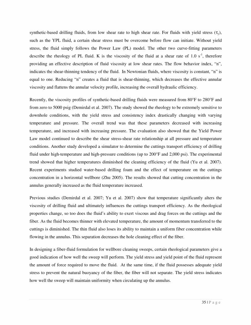
35 | P a g e

synthetic-based drilling fluids, from low shear rate to high shear rate. For fluids with yield stress (τy),

such as the YPL fluid, a certain shear stress must be overcome before flow can initiate. Without yield

stress, the fluid simply follows the Power Law (PL) model. The other two curve-fitting parameters

describe the rheology of PL fluid. K is the viscosity of the fluid at a shear rate of 1.0 s-1, therefore

providing an effective description of fluid viscosity at low shear rates. The flow behavior index, “n”,

indicates the shear-thinning tendency of the fluid. In Newtonian fluids, where viscosity is constant, “n” is

equal to one. Reducing “n” creates a fluid that is shear-thinning, which decreases the effective annular

viscosity and flattens the annular velocity profile, increasing the overall hydraulic efficiency.

Recently, the viscosity profiles of synthetic-based drilling fluids were measured from 80°F to 280°F and

from zero to 5000 psig (Demirdal et al. 2007). The study showed the rheology to be extremely sensitive to

downhole conditions, with the yield stress and consistency index drastically changing with varying

temperature and pressure. The overall trend was that these parameters decreased with increasing

temperature, and increased with increasing pressure. The evaluation also showed that the Yield Power

Law model continued to describe the shear stress-shear rate relationship at all pressure and temperature

conditions. Another study developed a simulator to determine the cuttings transport efficiency of drilling

fluid under high-temperature and high-pressure conditions (up to 200°F and 2,000 psi). The experimental

trend showed that higher temperatures diminished the cleaning efficiency of the fluid (Yu et al. 2007).

Recent experiments studied water-based drilling foam and the effect of temperature on the cuttings

concentration in a horizontal wellbore (Zhu 2005). The results showed that cutting concentration in the

annulus generally increased as the fluid temperature increased.

Previous studies (Demirdal et al. 2007; Yu et al. 2007) show that temperature significantly alters the

viscosity of drilling fluid and ultimately influences the cuttings transport efficiency. As the rheological

properties change, so too does the fluid’s ability to exert viscous and drag forces on the cuttings and the

fiber. As the fluid becomes thinner with elevated temperature, the amount of momentum transferred to the

cuttings is diminished. The thin fluid also loses its ability to maintain a uniform fiber concentration while

flowing in the annulus. This separation decreases the hole cleaning effect of the fiber.

In designing a fiber-fluid formulation for wellbore cleaning sweeps, certain rheological parameters give a

good indication of how well the sweep will perform. The yield stress and yield point of the fluid represent

the amount of force required to move the fluid. At the same time, if the fluid possesses adequate yield

stress to prevent the natural buoyancy of the fiber, the fiber will not separate. The yield stress indicates

how well the sweep will maintain uniformity when circulating up the annulus.

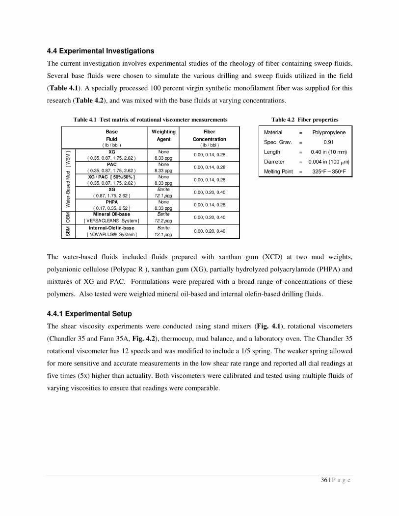
36 | P a g e

4.4 Experimental Investigations

The current investigation involves experimental studies of the rheology of fiber-containing sweep fluids.

Several base fluids were chosen to simulate the various drilling and sweep fluids utilized in the field

(Table 4.1). A specially processed 100 percent virgin synthetic monofilament fiber was supplied for this

research (Table 4.2), and was mixed with the base fluids at varying concentrations.

Table 4.1 Test matrix of rotational viscometer measurements

Table 4.2 Fiber properties

The water-based fluids included fluids prepared with xanthan gum (XCD) at two mud weights,

polyanionic cellulose (Polypac R ), xanthan gum (XG), partially hydrolyzed polyacrylamide (PHPA) and

mixtures of XG and PAC. Formulations were prepared with a broad range of concentrations of these

polymers. Also tested were weighted mineral oil-based and internal olefin-based drilling fluids.

4.4.1 Experimental Setup

The shear viscosity experiments were conducted using stand mixers (Fig. 4.1), rotational viscometers

(Chandler 35 and Fann 35A, Fig. 4.2), thermocup, mud balance, and a laboratory oven. The Chandler 35

rotational viscometer has 12 speeds and was modified to include a 1/5 spring. The weaker spring allowed

for more sensitive and accurate measurements in the low shear rate range and reported all dial readings at

five times (5x) higher than actuality. Both viscometers were calibrated and tested using multiple fluids of

varying viscosities to ensure that readings were comparable.

Base Weighting Fiber

Fluid Agent Concentration( lb / bbl ) ( lb / bbl )

XG None

( 0.35, 0.87, 1.75, 2.62 ) 8.33 ppg

PAC None

( 0.35, 0.87, 1.75, 2.62 ) 8.33 ppg

XG / PAC [ 50%/50% ] None

( 0.35, 0.87, 1.75, 2.62 ) 8.33 ppg

XG Barite

( 0.87, 1.75, 2.62 ) 12.1 ppg

PHPA None

( 0.17, 0.35, 0.52 ) 8.33 ppg

Mineral Oil-base Barite

[ VERSACLEAN® System ] 12.2 ppg

Internal-Olefin-base Barite

[ NOVAPLUS® System ] 12.1 ppgSB

M

0.00, 0.20, 0.40

OB

M

0.00, 0.14, 0.28

0.00, 0.20, 0.40

0.00, 0.14, 0.28

0.00, 0.14, 0.28

0.00, 0.14, 0.28

0.00, 0.20, 0.40

Wate

r-B

ased M

ud [ W

BM

]

Material = Polypropylene

Spec. Grav. = 0.91

Length = 0.40 in (10 mm)

Diameter = 0.004 in (100 μm)

Melting Point = 325°F – 350°F

Fig. 4.1 Stand mixers

4.4.2 Test Procedure

The steps required to prepare the samples and

Step 1. Preparation of Base Fluid:

and barite. Immediately after mixing, all water

a minimum of 24 hours to ensure full hydration. The fluids were then re

sample was obtained to determine the specific gravity using

Step 2. Preparation of Samples: After fluids were mixed and hydrated (if necessary), individual samples

were weighed and organized according to the polymer and fiber concentration. Fiber was added to

the samples at weight concentrations of 0.02,

water-based fluids, 0.08 percent

based and non-aqueous fluids it corresponded to 0.4 lb/bbl fiber.

Step 3. Viscometer Measurements at Ambient Tempera

rheologies of the base fluids were measured using two rotational viscometers (Chan

Fann 35A). If the viscosity of the fluid being measured exceeded the spring capacity of the

Chandler 35, the less sensitive but

measurements.

Step 4. Viscometer Measurements at High Temperature:

The oven was set at approximately 180°F, and samples were agitated every 15

uniformity. Once a sample was heated to 170°F as confirmed by a mercury thermometer, the

Fig. 4.2 Rotational viscometers

The steps required to prepare the samples and record measurements are as follows:

Preparation of Base Fluid: Bulk base fluid samples were prepared by mixing water, viscosifiers

and barite. Immediately after mixing, all water-based fluids were covered and left undisturbed for

a minimum of 24 hours to ensure full hydration. The fluids were then re-agitated, and a uniform

sample was obtained to determine the specific gravity using the mud balance.

After fluids were mixed and hydrated (if necessary), individual samples


the samples at weight concentrations of 0.02, 0.04, 0.06, and 0.08 percent. For the unweighted

percent corresponded to 0.28 lb/bbl fiber, whereas for the 12

aqueous fluids it corresponded to 0.4 lb/bbl fiber.

Viscometer Measurements at Ambient Temperature: After all samples were prepared, the

rheologies of the base fluids were measured using two rotational viscometers (Chan


tive but larger range Fann 35A was utilized for the higher shear rate

Viscometer Measurements at High Temperature: Samples were placed in an oven for heating.

The oven was set at approximately 180°F, and samples were agitated every 15


37 | P a g e

2 Rotational viscometers

Bulk base fluid samples were prepared by mixing water, viscosifiers,

based fluids were covered and left undisturbed for

agitated, and a uniform

After fluids were mixed and hydrated (if necessary), individual samples


. For the unweighted

corresponded to 0.28 lb/bbl fiber, whereas for the 12-ppg water-

After all samples were prepared, the

rheologies of the base fluids were measured using two rotational viscometers (Chandler 35 and


Fann 35A was utilized for the higher shear rate

Samples were placed in an oven for heating.

The oven was set at approximately 180°F, and samples were agitated every 15 minutes to ensure


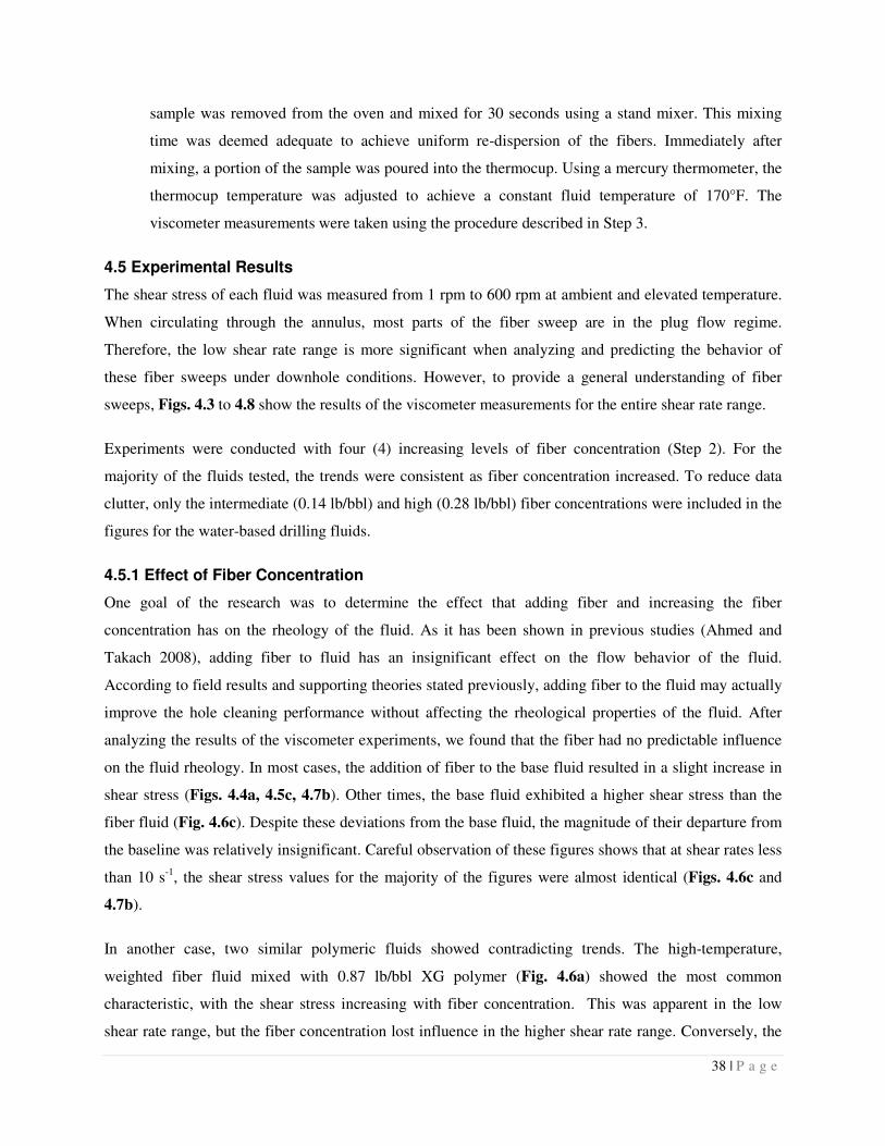
38 | P a g e

sample was removed from the oven and mixed for 30 seconds using a stand mixer. This mixing

time was deemed adequate to achieve uniform re-dispersion of the fibers. Immediately after

mixing, a portion of the sample was poured into the thermocup. Using a mercury thermometer, the

thermocup temperature was adjusted to achieve a constant fluid temperature of 170°F. The

viscometer measurements were taken using the procedure described in Step 3.

4.5 Experimental Results

The shear stress of each fluid was measured from 1 rpm to 600 rpm at ambient and elevated temperature.

When circulating through the annulus, most parts of the fiber sweep are in the plug flow regime.

Therefore, the low shear rate range is more significant when analyzing and predicting the behavior of

these fiber sweeps under downhole conditions. However, to provide a general understanding of fiber

sweeps, Figs. 4.3 to 4.8 show the results of the viscometer measurements for the entire shear rate range.

Experiments were conducted with four (4) increasing levels of fiber concentration (Step 2). For the

majority of the fluids tested, the trends were consistent as fiber concentration increased. To reduce data

clutter, only the intermediate (0.14 lb/bbl) and high (0.28 lb/bbl) fiber concentrations were included in the

figures for the water-based drilling fluids.

4.5.1 Effect of Fiber Concentration

One goal of the research was to determine the effect that adding fiber and increasing the fiber

concentration has on the rheology of the fluid. As it has been shown in previous studies (Ahmed and

Takach 2008), adding fiber to fluid has an insignificant effect on the flow behavior of the fluid.

According to field results and supporting theories stated previously, adding fiber to the fluid may actually

improve the hole cleaning performance without affecting the rheological properties of the fluid. After

analyzing the results of the viscometer experiments, we found that the fiber had no predictable influence

on the fluid rheology. In most cases, the addition of fiber to the base fluid resulted in a slight increase in

shear stress (Figs. 4.4a, 4.5c, 4.7b). Other times, the base fluid exhibited a higher shear stress than the

fiber fluid (Fig. 4.6c). Despite these deviations from the base fluid, the magnitude of their departure from

the baseline was relatively insignificant. Careful observation of these figures shows that at shear rates less

than 10 s-1, the shear stress values for the majority of the figures were almost identical (Figs. 4.6c and

4.7b).

In another case, two similar polymeric fluids showed contradicting trends. The high-temperature,

weighted fiber fluid mixed with 0.87 lb/bbl XG polymer (Fig. 4.6a) showed the most common

characteristic, with the shear stress increasing with fiber concentration. This was apparent in the low

shear rate range, but the fiber concentration lost influence in the higher shear rate range. Conversely, the

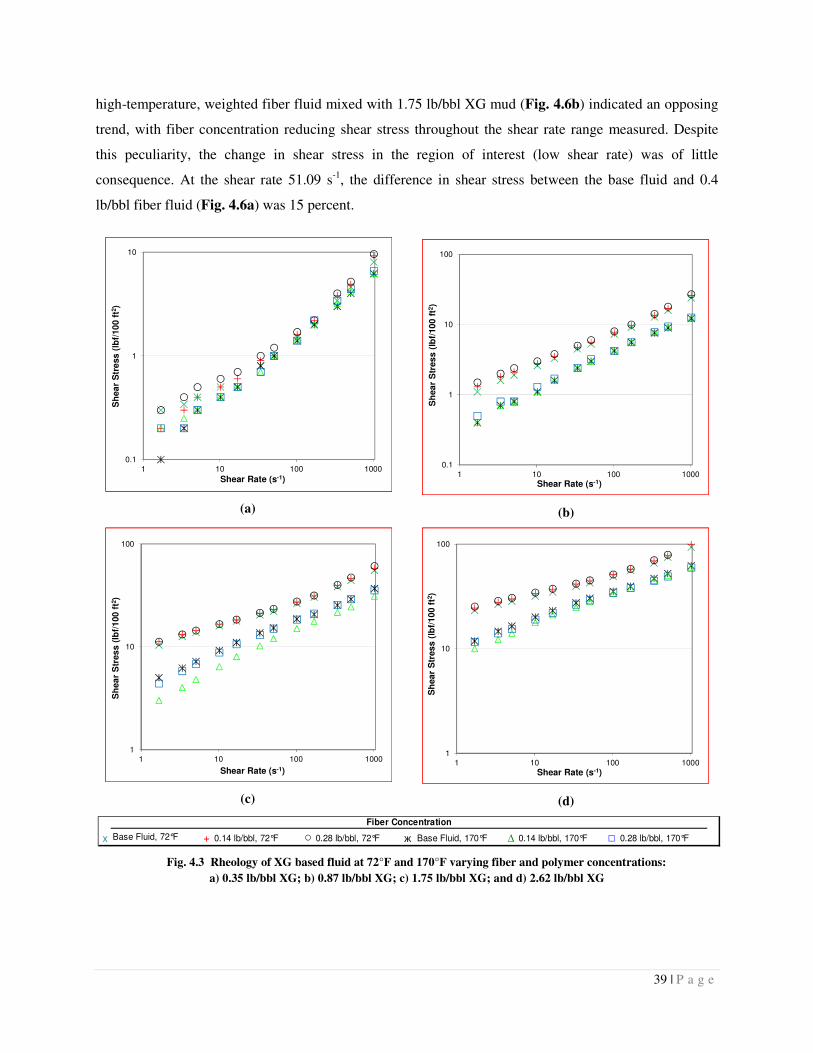
39 | P a g e

high-temperature, weighted fiber fluid mixed with 1.75 lb/bbl XG mud (Fig. 4.6b) indicated an opposing

trend, with fiber concentration reducing shear stress throughout the shear rate range measured. Despite

this peculiarity, the change in shear stress in the region of interest (low shear rate) was of little

consequence. At the shear rate 51.09 s-1, the difference in shear stress between the base fluid and 0.4

lb/bbl fiber fluid (Fig. 4.6a) was 15 percent.

(a)

(b)

(c)

(d)

Fig. 4.3 Rheology of XG based fluid at 72°F and 170°F varying fiber and polymer concentrations:

a) 0.35 lb/bbl XG; b) 0.87 lb/bbl XG; c) 1.75 lb/bbl XG; and d) 2.62 lb/bbl XG

0.1

1

10

1 10 100 1000

Sh

ea

r S

tre

ss

(lb

f/10

0 f

t2)

Shear Rate (s-1)

1

10

100

1 10 100 1000

Sh

ea

r S

tres

s (

lbf/

100

ft2

)

Shear Rate (s-1)

x Base Fluid, 72°F + 0.14 lb/bbl, 72°F ○ 0.28 lb/bbl, 72°F ж Base Fluid, 170°F ∆ 0.14 lb/bbl, 170°F □ 0.28 lb/bbl, 170°F

Fiber Concentration

0.1

1

10

100

1 10 100 1000

Sh

ea

r S

tres

s (

lbf/

10

0 f

t2)

Shear Rate (s-1)

1

10

100

1 10 100 1000

Sh

ea

r S

tres

s (

lbf/

10

0 f

t2)

Shear Rate (s-1)

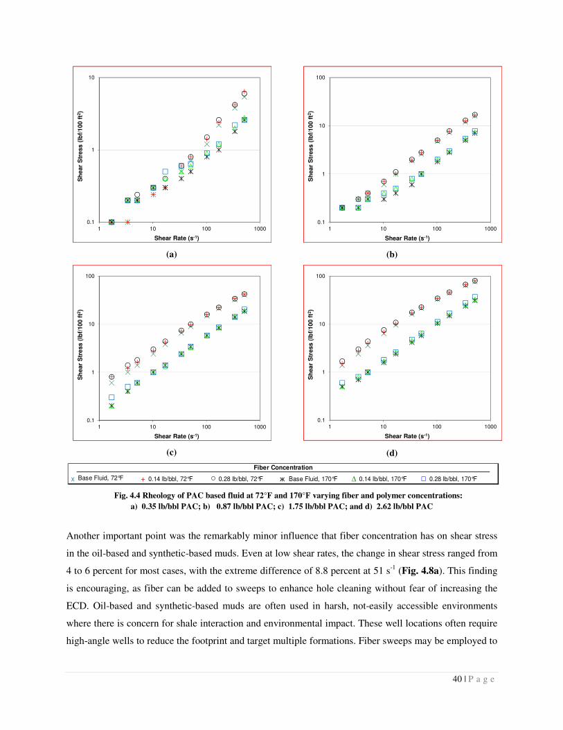
40 | P a g e

(a)

(b)

(c)

(d)

Fig. 4.4 Rheology of PAC based fluid at 72°F and 170°F varying fiber and polymer concentrations:

a) 0.35 lb/bbl PAC; b) 0.87 lb/bbl PAC; c) 1.75 lb/bbl PAC; and d) 2.62 lb/bbl PAC

Another important point was the remarkably minor influence that fiber concentration has on shear stress

in the oil-based and synthetic-based muds. Even at low shear rates, the change in shear stress ranged from

4 to 6 percent for most cases, with the extreme difference of 8.8 percent at 51 s-1 (Fig. 4.8a). This finding

is encouraging, as fiber can be added to sweeps to enhance hole cleaning without fear of increasing the

ECD. Oil-based and synthetic-based muds are often used in harsh, not-easily accessible environments

where there is concern for shale interaction and environmental impact. These well locations often require

high-angle wells to reduce the footprint and target multiple formations. Fiber sweeps may be employed to

0.1

1

10

1 10 100 1000

Sh

ear

Str

ess

(lb

f/1

00

ft2

)

Shear Rate (s-1)

0.1

1

10

100

1 10 100 1000

Sh

ear

Str

ess

(lb

f/10

0 f

t2)

Shear Rate (s-1)


Fiber Concentration

0.1

1

10

100

1 10 100 1000

Sh

ea

r S

tres

s (

lbf/

100

ft2

)

Shear Rate (s-1)

0.1

1

10

100

1 10 100 1000

Sh

ea

r S

tress

(lb

f/10

0 f

t2)

Shear Rate (s-1)

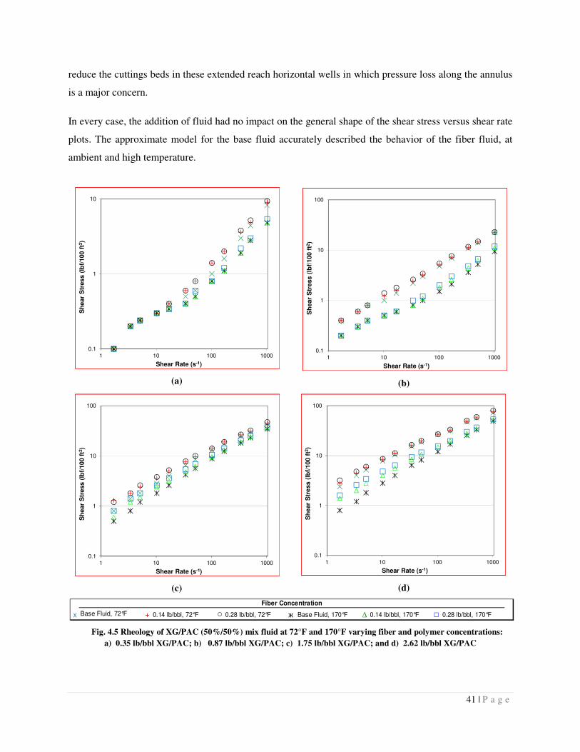
41 | P a g e

reduce the cuttings beds in these extended reach horizontal wells in which pressure loss along the annulus

is a major concern.

In every case, the addition of fluid had no impact on the general shape of the shear stress versus shear rate

plots. The approximate model for the base fluid accurately described the behavior of the fiber fluid, at

ambient and high temperature.

(a)

(b)

(c)

(d)

Fig. 4.5 Rheology of XG/PAC (50%/50%) mix fluid at 72°F and 170°F varying fiber and polymer concentrations:

a) 0.35 lb/bbl XG/PAC; b) 0.87 lb/bbl XG/PAC; c) 1.75 lb/bbl XG/PAC; and d) 2.62 lb/bbl XG/PAC

0.1

1

10

1 10 100 1000

Sh

ear

Str

es

s (

lbf/

100

ft2

)

Shear Rate (s-1)

0.1

1

10

100

1 10 100 1000

Sh

ear

Str

ess

(lb

f/1

00 f

t2)

Shear Rate (s-1)


Fiber Concentration

0.1

1

10

100

1 10 100 1000

Sh

ear

Str

ess

(lb

f/1

00 f

t2)

Shear Rate (s-1)

0.1

1

10

100

1 10 100 1000

Sh

ear

Str

ess

(lb

f/10

0 f

t2)

Shear Rate (s-1)

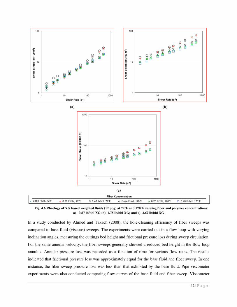
42 | P a g e

(a)

(b)

(c)

Fig. 4.6 Rheology of XG based weighted fluids (12 ppg) at 72°F and 170°F varying fiber and polymer concentrations:

a) 0.87 lb/bbl XG; b) 1.75 lb/bbl XG; and c) 2.62 lb/bbl XG

In a study conducted by Ahmed and Takach (2008), the hole-cleaning efficiency of fiber sweeps was

compared to base fluid (viscous) sweeps. The experiments were carried out in a flow loop with varying

inclination angles, measuring the cuttings bed height and frictional pressure loss during sweep circulation.

For the same annular velocity, the fiber sweeps generally showed a reduced bed height in the flow loop

annulus. Annular pressure loss was recorded as a function of time for various flow rates. The results

indicated that frictional pressure loss was approximately equal for the base fluid and fiber sweep. In one

instance, the fiber sweep pressure loss was less than that exhibited by the base fluid. Pipe viscometer

experiments were also conducted comparing flow curves of the base fluid and fiber sweep. Viscometer

1

10

100

1 10 100 1000

Sh

ea

r S

tre

ss

(lb

f/1

00

ft2

)

Shear Rate (s-1)

10

100

1000

1 10 100 1000

Sh

ear

Str

ess

(lb

f/10

0 f

t2)

Shear Rate (s-1)


Fiber Concentration

1

10

100

1 10 100 1000

Sh

ea

r S

tress

(lb

f/10

0 f

t2)

Shear Rate (s-1)

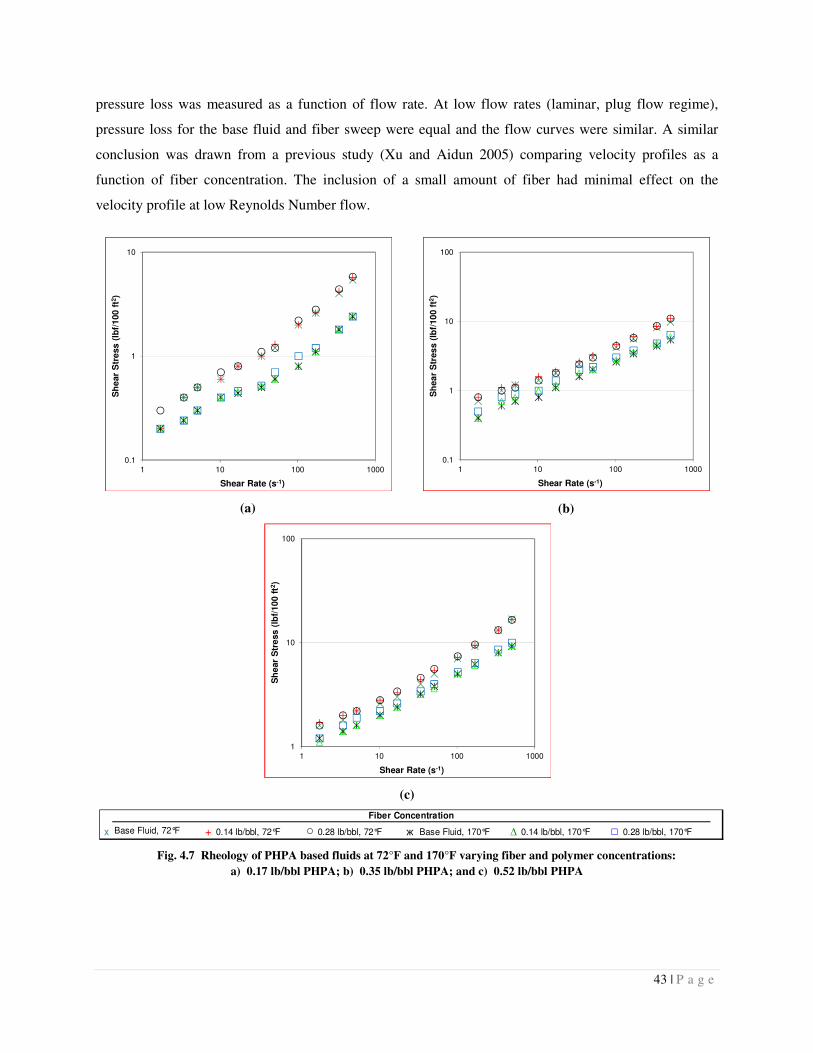
43 | P a g e

pressure loss was measured as a function of flow rate. At low flow rates (laminar, plug flow regime),

pressure loss for the base fluid and fiber sweep were equal and the flow curves were similar. A similar

conclusion was drawn from a previous study (Xu and Aidun 2005) comparing velocity profiles as a

function of fiber concentration. The inclusion of a small amount of fiber had minimal effect on the

velocity profile at low Reynolds Number flow.

(a)

(b)

(c)

Fig. 4.7 Rheology of PHPA based fluids at 72°F and 170°F varying fiber and polymer concentrations:

a) 0.17 lb/bbl PHPA; b) 0.35 lb/bbl PHPA; and c) 0.52 lb/bbl PHPA

0.1

1

10

1 10 100 1000

Sh

ear

Str

ess

(lb

f/1

00

ft2

)

Shear Rate (s-1)

1

10

100

1 10 100 1000

Sh

ear

Str

ess

(lb

f/10

0 f

t2)

Shear Rate (s-1)


Fiber Concentration

0.1

1

10

100

1 10 100 1000

Sh

ea

r S

tres

s (

lbf/

10

0 f

t2)

Shear Rate (s-1)

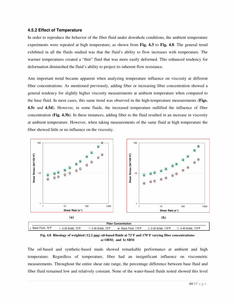
44 | P a g e

4.5.2 Effect of Temperature

In order to reproduce the behavior of the fiber fluid under downhole conditions, the ambient temperature

experiments were repeated at high temperature, as shown from Fig. 4.3 to Fig. 4.8. The general trend

exhibited in all the fluids studied was that the fluid’s ability to flow increases with temperature. The

warmer temperatures created a “thin” fluid that was more easily deformed. This enhanced tendency for

deformation diminished the fluid’s ability to project its inherent flow resistance.

Ann important trend became apparent when analyzing temperature influence on viscosity at different

fiber concentrations. As mentioned previously, adding fiber or increasing fiber concentration showed a

general tendency for slightly higher viscosity measurements at ambient temperature when compared to

the base fluid. In most cases, this same trend was observed in the high-temperature measurements (Figs.

4.5c and 4.5d). However, in some fluids, the increased temperature nullified the influence of fiber

concentration (Fig. 4.3b). In these instances, adding fiber to the fluid resulted in an increase in viscosity

at ambient temperature. However, when taking measurements of the same fluid at high temperature the

fiber showed little or no influence on the viscosity.

(a)

(b)

Fig. 4.8 Rheology of weighted (12.2 ppg) oil-based fluids at 72°F and 170°F varying fiber concentrations:

a) OBM; and b) SBM

The oil-based and synthetic-based muds showed remarkable performance at ambient and high

temperature. Regardless of temperature, fiber had an insignificant influence on viscometric

measurements. Throughout the entire shear rate range, the percentage difference between base fluid and

fiber fluid remained low and relatively constant. None of the water-based fluids tested showed this level

1

10

100

1 10 100 1000

Sh

ear

Str

es

s (

lbf/

10

0 f

t2)

Shear Rate (s-1)


Fiber Concentration

1

10

100

1 10 100 1000

Sh

ear

Str

es

s (

lbf/

100

ft2

)

Shear Rate (s-1)

45 | P a g e

of control over the entire shear rate range at both temperatures.

The temperature of the fluids was altered to provide a closer representation to actual downhole conditions.

However, elevated pressure conditions in the wellbore were not considered in this study, partly as a

consequence of the operational capability of the equipment available for these experiments. Previous

studies investigated the effect of elevated pressure on the rheology of various fluids. Zhou et al. (2004)

conducted experiments to investigate aerated mud cuttings transport in an HPHT flow loop. The effect of

elevated pressure (up to 500 psi) was found to have minimal influence on cuttings concentration.

Another study (Alderman et al. 1988) investigated the influence of high temperature and high pressure on

water-based mud. The viscous behavior of the fluids in the HPHT conditions reflected the characteristics

of their respective continuous phases: a weak pressure dependence and an exponential temperature

dependence. It was also shown that the fluid yield stress was essentially independent of pressure, but

highly influenced by temperature. Other studies concentrating on the pressure and temperature effects on

cement slurry rheology gave similar results. The plastic viscosity of the cement slurry showed little

increase with increasing pressure (up to 5000 psi) in relation to the significant effect of increased

temperature up to 260°F (Ravi and Sutton 1990).

4.5.3 Shear Viscosity Parameters

The first step in analyzing the fiber fluid shear viscosity was to record all the viscometer shear stress

measurements. Least-square regression was performed to determine the rheological parameters for all

fluid-fiber-temperature formulations (Tables 4.3 through 4.8). The coefficient of determination, R2,

represents how well the measured shear stress values correlate with the values predicted by the Yield

Power Law model. An R2 value of 1.00 represents an exact match of experimental data with the

predictive model data. The vast majority of the experimental data points fit the regression model

extremely well.

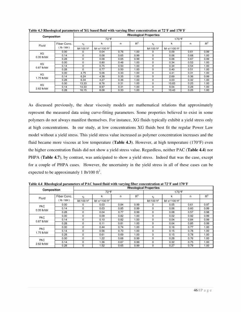
46 | P a g e

Table 4.3 Rheological parameters of XG based fluid with varying fiber concentration at 72°F and 170°F

As discussed previously, the shear viscosity models are mathematical relations that approximately

represent the measured data using curve-fitting parameters. Some properties believed to exist in some

polymers do not always manifest themselves. For instance, XG fluids typically exhibit a yield stress only

at high concentrations. In our study, at low concentrations XG fluids best fit the regular Power Law

model without a yield stress. This yield stress value increased as polymer concentration increases and the

fluid became more viscous at low temperature (Table 4.3). However, at high temperature (170°F) even

the higher concentration fluids did not show a yield stress value. Regardless, neither PAC (Table 4.4) nor

PHPA (Table 4.7), by contrast, was anticipated to show a yield stress. Indeed that was the case, except

for a couple of PHPA cases. However, the uncertainty in the yield stress in all of these cases can be

expected to be approximately 1 lb/100 ft2.

Table 4.4 Rheological parameters of PAC based fluid with varying fiber concentration at 72°F and 170°F

τy k n R2τy k n R2

lbf /100 ft2 lbf-sn/100 ft2 lbf /100 ft2 lbf-sn/100 ft2

0.00 0 0.04 0.76 1.00 0 0.09 0.61 0.99

0.14 0 0.08 0.65 0.99 0 0.06 0.68 1.00

0.28 0 0.08 0.65 0.99 0 0.06 0.67 0.99

0.00 0 0.80 0.48 1.00 0 0.34 0.53 1.00

0.14 0 0.75 0.50 1.00 0 0.34 0.54 1.00

0.28 0 0.77 0.50 1.00 0 0.40 0.51 1.00

0.00 4.75 5.06 0.33 1.00 0 4.41 0.31 1.00

0.14 6.24 4.38 0.35 1.00 0 2.69 0.36 0.99

0.28 6.34 4.27 0.36 1.00 0 4.03 0.32 1.00

0.00 13.33 8.76 0.31 1.00 0 10.83 0.25 1.00

0.14 14.33 8.97 0.31 1.00 0 9.04 0.28 1.00

0.28 16.15 8.08 0.33 1.00 0 10.43 0.25 1.00

Rheological Properties

72°F 170°FComposition

XG

1.75 lb/bbl

XG

2.62 lb/bbl

FluidFiber Conc.

( lb / bbl )

XG

0.35 lb/bbl

XG

0.87 lb/bbl



0.00 0 0.03 0.84 0.99 0 0.05 0.61 0.97

0.14 0 0.03 0.85 0.99 0 0.06 0.60 0.99

0.28 0 0.04 0.77 0.99 0 0.08 0.57 0.98

0.00 0 0.09 0.82 1.00 0 0.02 0.92 0.99

0.14 0 0.10 0.82 1.00 0 0.04 0.84 0.99

0.28 0 0.11 0.81 1.00 0 0.04 0.85 0.99

0.00 0 0.44 0.74 1.00 0 0.16 0.77 1.00

0.14 0 0.56 0.70 1.00 0 0.15 0.78 1.00

0.28 0 0.61 0.69 1.00 0 0.15 0.78 1.00

0.00 0 1.22 0.68 0.99 0 0.28 0.76 1.00

0.14 0 1.36 0.67 0.99 0 0.32 0.75 1.00

0.28 0 1.52 0.65 0.99 0 0.27 0.79 1.00

72°F


170°F

FluidFiber Conc.

( lb / bbl )

Composition

PAC

0.35 lb/bbl

PAC

0.87 lb/bbl

PAC

1.75 lb/bbl

PAC

2.62 lb/bbl

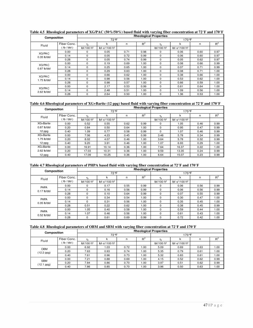
47 | P a g e

Table 4.5 Rheological parameters of XG/PAC (50%/50%) based fluid with varying fiber concentration at 72°F and 170°F

Table 4.6 Rheological parameters of XG+Barite (12 ppg) based fluid with varying fiber concentration at 72°F and 170°F

Table 4.7 Rheological parameters of PHPA based fluid with varying fiber concentration at 72°F and 170°F

Table 4.8 Rheological parameters of OBM and SBM with varying fiber concentration at 72°F and 170°F

τy k n R2 τy k n R

2


0.00 0 0.05 0.71 0.98 0 0.06 0.60 0.97

0.14 0 0.05 0.72 0.99 0 0.06 0.60 0.97

0.28 0 0.05 0.74 0.99 0 0.05 0.62 0.97

0.00 0 0.19 0.69 1.00 0 0.08 0.66 0.99

0.14 0 0.25 0.65 1.00 0 0.07 0.71 0.99

0.28 0 0.29 0.63 1.00 0 0.08 0.71 1.00

0.00 0 0.66 0.62 1.00 0 0.38 0.66 1.00

0.14 0 0.98 0.56 1.00 0 0.53 0.62 1.00

0.28 0 0.98 0.57 1.00 0 0.66 0.59 1.00

0.00 0 2.17 0.53 0.99 0 0.61 0.64 1.00

0.14 0 2.48 0.51 1.00 0 1.09 0.56 1.00

0.28 0 2.64 0.50 1.00 0 1.36 0.53 1.00

Composition170°F72°F


XG/PAC

0.35 lb/bbl

XG/PAC

0.87 lb/bbl

XG/PAC

1.75 lb/bbl

XG/PAC

2.62 lb/bbl

FluidFiber Conc.

( lb / bbl )



XG+Barite 0.00 0.52 0.55 0.62 0.99 0 1.05 0.46 0.99

0.87 lb/bbl 0.20 0.84 0.50 0.64 1.00 0 0.95 0.47 0.99

12 ppg 0.40 1.09 0.77 0.58 0.99 0 1.07 0.46 0.99

XG+Barite 0.00 7.06 4.23 0.45 0.99 3.48 5.78 0.34 0.99

1.75 lb/bbl 0.20 8.02 4.07 0.46 1.00 3.64 5.78 0.32 0.99

12 ppg 0.40 9.20 3.91 0.46 1.00 1.07 6.93 0.29 1.00

XG+Barite 0.00 16.91 10.14 0.36 1.00 7.64 16.37 0.22 1.00

2.62 lb/bbl 0.20 17.03 10.31 0.36 1.00 9.59 13.35 0.24 0.99

12 ppg 0.40 17.09 10.25 0.36 1.00 6.64 15.07 0.23 0.99

72°F


170°F

FluidFiber Conc.

( lb / bbl )

Composition



0.00 0 0.17 0.55 0.99 0 0.06 0.56 0.99

0.14 0 0.16 0.56 0.99 0 0.06 0.56 0.99

0.28 0 0.10 0.64 0.99 0 0.07 0.55 0.99

0.00 0 0.34 0.54 1.00 0 0.30 0.47 1.00

0.14 0 0.31 0.56 1.00 0 0.35 0.45 1.00

0.28 0.51 0.22 0.62 1.00 0 0.38 0.45 0.99

0.00 1.05 0.40 0.58 1.00 0 0.59 0.44 1.00

0.14 1.07 0.46 0.56 1.00 0 0.61 0.43 1.00

0.28 0 0.61 0.69 0.99 0 0.72 0.42 1.00

PHPA

0.17 lb/bbl


FluidFiber Conc.

( lb / bbl )


PHPA

0.35 lb/bbl

PHPA

0.52 lb/bbl

τy k n R2

τy k n R2


0.00 6.92 1.03 0.72 1.00 5.09 0.69 0.63 1.00

0.20 7.63 0.93 0.74 1.00 5.35 0.79 0.61 1.00

0.40 7.61 0.96 0.73 1.00 5.32 0.83 0.61 1.00

0.00 7.21 0.88 0.69 1.00 4.15 0.52 0.62 0.99

0.20 7.84 0.86 0.70 1.00 3.97 0.51 0.62 0.99

0.40 7.86 0.85 0.70 1.00 3.96 0.50 0.63 1.00



FluidFiber Conc.

( lb / bbl )

OBM

(12.2 ppg)

SBM

(12.1 ppg)

48 | P a g e

4.6 Conclusions

This study was conducted to investigate the effects of temperature and fiber concentration on the rheology

of fiber-containing sweeps. Rheology experiments were conducted using rotational viscometers to

measure the rheology of base fluids and fiber-containing fluids at ambient temperature and 170°F. The

shear viscosity profiles of fiber sweep fluids were compared using graphical and curve-fitting regression

analyses. Based on the experimental results and data analysis, the following conclusions were made:

• The addition of fiber up to 0.08 weight percent has a minor effect on the fluid’s shear viscosity

profile, whether at ambient temperature or 170°F. Some instances showed slight increases in

viscosity, while others showed a decrease with increasing fiber concentration.

• Increasing the temperature of the fluid decreased the non-Newtonian behavior of the fiber fluid

and decreased the viscosity throughout the shear rate range of 2 to 1000s-1.

• In most cases, as fiber concentration increased, the viscosity showed increasingly non-Newtonian

behavior: in the Yield Power Law model, n decreased while K and τy increased.

• Neither oil-based nor synthetic-based fluids exhibited any significant shear viscosity sensitivity to

fiber concentration at ambient temperature or at 170°F. It may be possible for oil-based or

synthetic-based mud sweeps to be utilized in the field with no increase in ECD.

Nomenclature

BHA = Bottomhole Assembly

BP = Bingham Plastic


ERD = Extended reach drilling

K = Consistency index (lbf-sn/100 ft2)

N = Flow behavior index

ppg = Pounds per gallon

PAC = Polyanionic Cellulose

PHPA = Partially Hydrolyzed Polyacrylamide

PL =Power Law

XG = Xanthan Gum

YPL =Yield Power Law

Greek Letters

τ = Shear stress (lbf/100 ft2)

τy = Yield stress (lbf/100 ft2)

49 | P a g e

γ = shear rate (s-1)

µ = Viscosity

References

Ahmed, R.M. and Takach, N.E. 2008. Fiber Sweeps for Hole Cleaning. Paper SPE 113746 presented at

the SPE/ICoTA Coiled Tubing and Well Intervention Conference and Exhibition, The Woodlands,

Texas, 1-2 April. DOI: 10.2118/113746-MS.

Alderman, N.J., Gavignet, A., Guillot, D. and Maitland, G.C. 1998. High-Temperature, High-Pressure

Rheology of Water-Based Muds. Paper SPE 18035 presented at the SPE Annual Technical

Conference and Exhibition, Houston, Texas, October 2-5. DOI: 10.2118/18035-MS.

Bivins, C.H., Boney, C., Fredd, C., Lassek, J. Sullivan, P., Engels, J., Fielder, E.O. et al. 2005. New

Fibers for Hydraulic Fracturing. Schlumberger Oilfield Review 17 (2): 34-43.

Bulgachev, R.V. and Pouget, P. 2006. New Experience in Monofilament Fiber Tandem Sweeps Hole

Cleaning Performance on Kharyaga Oilfield, Timan-Pechora Region of Russia. Paper SPE 101961

presented at the SPE Russian Oil and Gas Technical Conference and Exhibition, Moscow, Russia, 3-6

October. DOI: 10.2118/101961-MS.

Cameron C. 2001. Drilling Fluids Design and Management for Extended Reach Drilling. Paper SPE

72290 presented at the IADC/SPE Middle East Drilling Technology conference, Bahrain, 22-24

October. DOI: 10.2118/72290-MS.

Cameron, C., Helmy, H., and Haikal, M. 2003. Fibrous LCM Sweeps Enhance Hole Cleaning and ROP

on Extended Reach Well in Abu Dhabi. Paper SPE 81419 presented at the SPE 13th Middle East Oil

Show and Conference, Bahrain, 5-8 April. DOI: 10.2118/81419-MS.

Demirdal, B., Miska, S., Takach, N.E. and Cunha, J.C. 2007. Drilling Fluids Rheological and Volumetric

Characterization Under Downhole Conditions. Paper SPE 108111 presented at the SPE Latin

American and Caribbean Petroleum Engineering Conference, Buenos Aires, Argentina, 15-18 April.

DOI: 10.2118/108111-MS.

Drilling Fluid Rheology. 2001. Kelco Oil Field Group, Houston, Texas (Rev. Sep 2005).

Gupta, V.K., Sureshkumar, R., Khomami, B. and Azaiez, J. 2002. Centrifugal Instability of Semidilute

non-Brownian Fiber Suspensions. Physics of Fluids 14 (6): 1958-1971

Hemphill, T. and Rojas, J.C. 2002. Drilling Fluid Sweeps: Their Evaluation, Timing, and Applications.

Paper SPE 77448 presented at the SPE Annual Technical Conference and Exhibition, San Antonio,

Texas, 29 September-2 October. DOI: 10.2118/77448-MS.

Maehs, J., Renne, S., Logan, B. and Diaz, N. 2010. Proven Methods and Techniques to Reduce Torque

and Drag in the Pre-Planning and Drilling Execution of Oil and Gas Wells. Paper SPE 128329

50 | P a g e

presented at the IADC/SPE Drilling Conference and Exhibition, New Orleans, Louisiana, 2-4

February. DOI: 10.2118/128329-MS.

Power, D.J., Hight, C., Weisinger, D. and Rimer, C. 2000. Drilling Practices and Sweep Selection for

Efficient Hole Cleaning in Deviated Wellbores. Paper SPE 62794 presented at the IADC/SPE Asia

Pacific Drilling Technology conference, Kuala Lumpur, Malaysia, 11-13 September. DOI:

10.2118/62794-MS.

Ravi, K.M. and Sutton, D.L. 1990. New Rheological Correlation for Cement Slurries as a Function of

Temperature. Paper SPE 20449 presented at the SPE Annual Technical Conference and Exhibition,

New Orleans, Louisiana, 23-26 September. DOI: 10.2118/20449-MS.

Robertson, N., Hancock, S., and Mota, L. 2005. Effective Torque Management of Wytch Farm

Extended-Reach Sidetrack Wells. Paper SPE 95430 presented at the SPE Annual Technical

Conference and Exhibition, Dallas, Texas, 9-12 October. DOI: 10.2118/95430-MS.

Swerin, A. 1997. Rheological properties of cellulosic fibre suspensions flocculated by cationic

polyacrylamides. Colloids and Surfaces A: Physiochemical and Engineering Aspects 133 (3): 279-

294

Valluri, S.G., Miska, S.Z., Ahmed, R.M. and Takach, N.E. 2006. Experimental Study of Effective Hole

Cleaning Using “Sweeps” in Horizontal Wellbores. Paper SPE 101220 presented at the SPE Annual

Technical Conference and Exhibition, San Antonio, Texas, 24-27 September. DOI: 10.2118/101220-

MS.

Xu, A.H. and Aidun, C. K. “Characteristics of fiber suspension flow in a rectangular channel,”

International Journal of Multiphase Flow 31 (2005) 318–336.

Yu, M., Takach, N.E., Nakamura, D.R. and Shariff, M.M. 2007. An Experimental Study of Hole Cleaning

Under Simulated Downhole Conditions. Paper SPE 109840 presented at the SPE Annual Technical

Conference and Exhibition, Anaheim, California, 11-14ovember. DOI: 10.2118/109840-MS.

Zhou, L., Ahmed, R.M., Miska, S.Z., Takach, N.E., Yu, M., and Pickell, M.B. 2004. Experimental Study

& Modeling of Cuttings Transport with Aerated Mud in Horizontal Wellbore at Simulated Downhole

Conditions. Paper SPE 90038 presented at the SPE Annual Technical Conference and Exhibition,

Dallas, Texas, 26-29 September. DOI: 10.2118/90038-MS.

Zhu, C. 2005. Cuttings Transport with Foam in Horizontal Concentric Annulus Under Elevated Pressure

and Temperature Conditions. Ph.D. Dissertation, University of Tulsa, Tulsa, Oklahoma.

51 | P a g e

5. Settling Behavior of Particles in Fiber-containing Drilling Fluids

Fiber-containing fluids are utilized in many industrial applications. In the upstream petroleum industry,

fiber suspensions are used to transport rock cuttings from the bottom of the hole to the surface. Moreover,

fibrous fluids are applied in fracturing operations to transport proppant particle to the fractured space.

Solids transport performances of these fluids largely depends on the settling behavior of suspended

particles.

This section of the report presents results of experimental and theoretical investigations conducted on the

settling behavior of spherical particles in fiber-containing fluid. Settling experiments were carried out in a

4-inch fully transparent cylinder that is sufficiently long (6.5 feet) to establish terminal settling conditions.

Both Newtonian and non-Newtonian fluids were considered in the investigation. A moving digital camera

system was used to track and locate a particle while it was settling in fully transparent test fluid. The

camera records were used to determine the settling velocity of each particle as a function of time. Tests

were performed with particles that have different sizes (2 mm to 8 mm). Fiber concentration was varied

from 0.00 to 0.08 percent by weight.

When a particle settles in the fibrous fluid, it experiences fiber drag in addition to the conventional

hydrodynamic resistance (i.e., viscous drag). Measured terminal velocity was used to compute the

viscous component of the total drag. Subsequently, applying the momentum balance, the fiber drag

component acting on the particle was determined from the total drag. Results showed that the fiber drag

was a function of the projection area of the particle, settling velocity, fiber drag coefficient, and density

difference between the fluid and particle. The fiber drag coefficient varied with Reynolds Number, fiber

concentration, and fluid behavior index. Using the experimental data, a semi-empirical model was

developed to predict terminal settling velocity of a particle in fiber-containing fluids. The correlation was

validated for both Newtonian and non-Newtonian base fluids that have low concentrations of hole-

cleaning fibers. The correlation is applicable to suspensions containing fully dispersed fibers with length

of approximately 10 mm and diameter of 100 µm.

5.1 Introduction

Settling and sedimentation occur in many areas of the petroleum industry and process engineering

operations. Typical applications of settling velocity include drill cuttings and proppants, transport

prediction, design of separators and settling tanks, and hydraulic and pneumatic transportation of solids

particle in mining, coal, and other industrial applications.

52 | P a g e

Studies on settling velocity of solids particles in Newtonian and non-Newtonian fluids have been well-

documented (Shah 1982; Klessidis 2004; Chhabbra & Peri 1991; Dallon 1967; Prakash 1983; Lali et al.

1989; and Chhabra 1980). Shah (1982) developed a new approach to analyze proppant settling in non-

Newtonian fluid. The study showed that the drag coefficient correlation is a function of Reynolds Number

and fluid behavior index ”n”. Especially at low Reynolds numbers, the fluid behavior index “n” has a

significant effect on the proppant settling velocity and this effect diminishes at high Reynolds Numbers. It

also shows that the correlation developed for static settling velocity can predict the dynamic settling data.

It was recommended to plot C�� versus Reynolds Number to get a better curve fit with a single straight

line on a log-log plot. The method had been tested (Shah et al. 2007) with data from the previous studies

(Dallon 1967; Prakash 1983; Lali et al. 1989; and Chhabra 1980) and satisfactory agreements had been

obtained. An experimental study (Fang 1992) conducted on free settling of spherical particles in

Newtonian and non-Newtonian fluids showed both stable and swinging settling patterns.

Particles in fluids with yield stress show different settling behavior. Fine and/or light particles can fully

suspend in the fluid due the yield stress. Dedegil (1987) developed a method to predict settling velocity

of particles in Herschel-Bulkley (Yield Power Law) fluid. The method relates the drag coefficient to the

generalized Reynolds Number based on apparent viscosity calculated from the representative shear rate

(V/d). The method accounts for the effect of yield stress on the settling velocity. It condensed most of the

published data (Valentik and Whitmore 1965) into a single curve when the drag coefficient was plotted

against the generalized Reynolds Number.

Many of the fluids used in the industry exhibit viscoelastic behavior. A study (Acharga 1986) conducted

on particle settling in viscoelastic fluid indicated that the fluid elasticity does not affect the settling rate in

the creeping flow region (low Reynolds Number). However, it enhances the sedimentation rate in the

transition zone. Predictions from a theoretical model were compared with measurements and showed

good agreement. Drag coefficient is strongly influenced by viscoelastic properties of the fluid.

Experiments (Jin and Penny 1995) revealed the variation of drag coefficient with the Reynolds Number

(NRep) and dimensionless viscoelastic parameter of the test fluid. In addition to fluid properties, the shape

of a particle has substantial effect on its settling behavior. Empirical models (Peden and Luo 1987; Chien

1994) developed to predict settling velocities of non-spherical particles showed the relationship between

the drag coefficient and shape factor.

Furthermore, the presence of a wall can create hydrodynamic interference with the settling particles. As

particles settle in fluids, their motion is affected by the presence of other particles and/or container walls.

The wall effect tends to reduce the settling velocity. The hydrodynamic effects of container walls have

53 | P a g e

been investigated (Brown et al. 1950; Lali et al. 1988; Di Felice et al. 1995) extensively. Experiments

(Lali et al. 1988 and Brown et al. 1950) showed that the diameter ratio (i.e., the ratio of the diameter of

the container to the diameter of the particle) and Reynolds Number determines the wall effect. Empirical

correlations are available to determine correction factors that account for the presence of a wall. These

factors relate the wall-free settling velocity to the actual velocity under both laminar and turbulent

conditions.

The presence of neighboring particles creates hydrodynamic interference that hinders particle

sedimentation. A number of experimental and theoretical studies (Richardson and Zaki 1954; Govier and

Aziz 1972; Smith 1997; Daneshy 1978) were conducted to investigate sedimentation in concentrated

suspensions, which demonstrated the reduction of settling velocity at high solids concentrations.

Increasing the particle concentration tends to increase the hydrodynamic interference and particle

collision, which are highly dependent on the flow regime (Govier and Aziz 1972). Uniformly-sized

particles in laminar motion have identical velocities, and collision is not expected even as concentration

increases. However, in turbulent flow collisions can occur due to settling speed differences that arise from

random fluctuations of fluid velocity. Moreover, in actual situations the solids particles do not have

uniform size distribution. As a result, even under laminar conditions, particle collision can exist. The

collisions intensify with the increase in particle concentration and differences in particle settling speeds.

Smith (1998) developed a theoretical model to predict the sedimentation velocity of uniformly-sized

particles in Newtonian fluid under laminar conditions. The model was compared with the correlation of

Richardson and Zaki (1954). Even though general agreement was obtained at high concentrations,

discrepancies were observed at low concentrations.

Rheological behavior of fiber suspensions is very complex. The introduction of fiber can significantly

alter the fluid rheology. Rajabian et al. (2008) developed a rheological model for fiber-containing

polymer suspensions. The model includes the fiber-fiber and fiber-polymer interaction. The experimental

measurements obtained from simple shear flows agreed with the model predictions. Another study of

fiber suspensions (Marti et al. 2005) showed minor gains in viscosity as the fiber concentration was

incrementally increased from an initial dilute suspension. However, at higher fiber concentrations, the

viscosity showed greater sensitivity to fiber concentration.

In the drilling industry, sweep fluid is used to improve wellbore cleaning in inclined and horizontal wells

when the regular drilling fluid fails to clean the wellbore sufficiently. Conventional sweeps are commonly

categorized as i.) high-viscosity; ii.) high-density; iii.) low-viscosity; iv.) combination; and v.) tandem

sweeps (Hemphill 2002). Sweeps provide a number of benefits, such as reducing cuttings beds and

54 | P a g e

subsequent decrease in annular pressure loss, as well as a reduction in torque and drag at the surface. As

a result, it is often applied to reduce excessive annular pressure losses and clean the wellbore prior to

tripping operation. Hole cleaning fiber is added to the sweep fluid to improve its performance with a

negligible increase in viscosity and pressure loss. Previous studies (Ahmed and Takach 2008; Cameron

et al. 2003; Bulgachev & Pouget 2006) reported that adding a small amount of hole cleaning fiber (less

than 0.1 percent by weight) improves solid transport performance of the sweep with no noticeable change

in fluid rheology.

Fiber has also shown considerable promise in well stimulation operations. Hydraulic fracturing requires

extremely high downhole fluid pressure to induce cracks into the reservoir rock, fracturing the formation.

A material that can withstand highly compressive forces, proppant, is necessary to prevent the fractures

from closing after the fluid pressure subsides and hydrocarbon production begins. As the fracturing fluid

is pumped downhole, the proppant travels with and behind it, and remains in the fracture after the fluid is

imbibed into the formation and/or flows back. With insufficient particle suspension properties, the

fracturing fluid will allow the proppant to settle before the fracture face closes and reduce the uniformity

and effectiveness of the proppant within the fracture. Conventional fracturing fluids rely on viscosity for

particle suspension, which precipitate excessive pressure losses and consequently require high pump

pressures. Fiber has been added to stimulation fluids to achieve the suspension properties necessary to

transport and deposit the proppant as designed, ensuring desired fracture conductivity and overall

productivity of the well. The fiber fluid can achieve equivalent suspension characteristics with less

viscosity, therefore requiring less pressure during stimulation operations. An experimental investigation

was conducted to evaluate the benefits of using fiber to prevent proppant settling in hydraulic fractures

(Bivins et al. 2005). Results showed a substantial reduction in the proppant settling velocity, which was

attributed to fiber concentration.

The settling behavior of particles in fiber suspensions is more complex than in the base fluid (i.e., fluid

without suspension). The interactions among the fiber particles, suspended solids and base fluid are

difficult, if not impossible, to express mathematically. When the fiber is fully dispersed in fluid, it can

form a stable network structure. The strength of the network depends on the fiber concentration and

length. Suspensions with low fiber concentrations and/or short fiber length form a very weak network.

The network structure created by the fiber particles tends to reduce the settling velocity of dense particles

due to fiber-fiber and fiber-particle interactions. The origins of these interactions can be mechanical

contact and/or hydrodynamic interference between fiber particles. Mechanical contact between fiber

particles generate a strong friction force that hinders the settling of suspended particles or drill cuttings. A

numerical investigation was conducted to study the settling of a small sphere through a suspension of

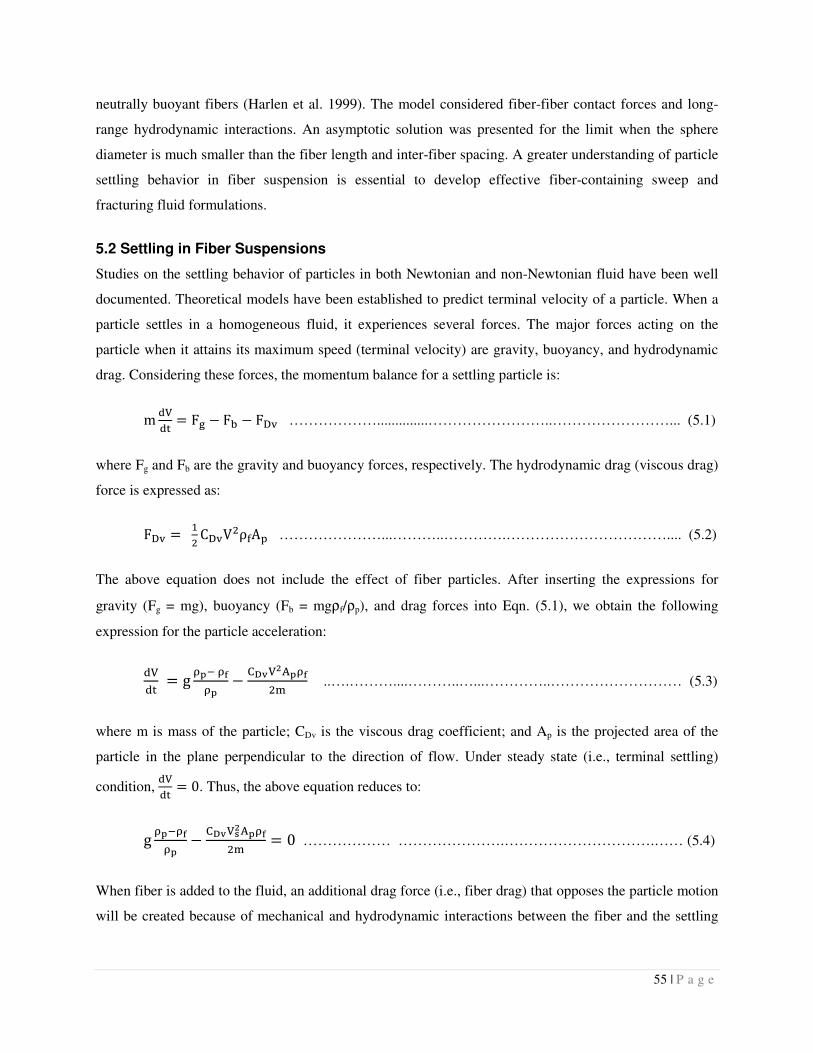
55 | P a g e

neutrally buoyant fibers (Harlen et al. 1999). The model considered fiber-fiber contact forces and long-

range hydrodynamic interactions. An asymptotic solution was presented for the limit when the sphere

diameter is much smaller than the fiber length and inter-fiber spacing. A greater understanding of particle

settling behavior in fiber suspension is essential to develop effective fiber-containing sweep and

fracturing fluid formulations.

5.2 Settling in Fiber Suspensions

Studies on the settling behavior of particles in both Newtonian and non-Newtonian fluid have been well

documented. Theoretical models have been established to predict terminal velocity of a particle. When a

particle settles in a homogeneous fluid, it experiences several forces. The major forces acting on the

particle when it attains its maximum speed (terminal velocity) are gravity, buoyancy, and hydrodynamic

drag. Considering these forces, the momentum balance for a settling particle is:

m �� F� � F� � F�� ………………..............……………………..……………………... (5.1)

where Fg and Fb are the gravity and buoyancy forces, respectively. The hydrodynamic drag (viscous drag)

force is expressed as:

F�� C��V�ρ�A� …………………...………..………….…………………………….... (5.2)

The above equation does not include the effect of fiber particles. After inserting the expressions for

gravity (Fg = mg), buoyancy (Fb = mgρf/ρp), and drag forces into Eqn. (5.1), we obtain the following

expression for the particle acceleration:

�� g �� !"��# ..….………....………..…...…………..……………………… (5.3)

where m is mass of the particle; CDv is the viscous drag coefficient; and Ap is the projected area of the

particle in the plane perpendicular to the direction of flow. Under steady state (i.e., terminal settling)

condition, �� 0. Thus, the above equation reduces to:

g �� %!"��# 0 ……………… ………………….………………………….…… (5.4)

When fiber is added to the fluid, an additional drag force (i.e., fiber drag) that opposes the particle motion

will be created because of mechanical and hydrodynamic interactions between the fiber and the settling

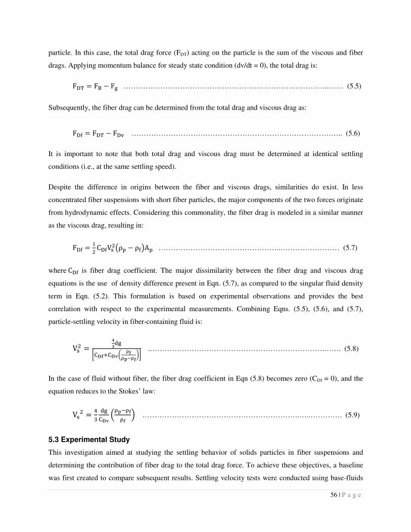
56 | P a g e

particle. In this case, the total drag force (FDT) acting on the particle is the sum of the viscous and fiber

drags. Applying momentum balance for steady state condition (dv/dt = 0), the total drag is:

F�& F' � F� …………………………………………………………….…………..…… (5.5)

Subsequently, the fiber drag can be determined from the total drag and viscous drag as:

F�� F�& � F�� ………………………………………………………………………….. (5.6)

It is important to note that both total drag and viscous drag must be determined at identical settling

conditions (i.e., at the same settling speed).

Despite the difference in origins between the fiber and viscous drags, similarities do exist. In less

concentrated fiber suspensions with short fiber particles, the major components of the two forces originate

from hydrodynamic effects. Considering this commonality, the fiber drag is modeled in a similar manner

as the viscous drag, resulting in:

F�� C��V(�)ρ� � ρ�*A� …………………………………………..…………………… (5.7)

whereC�� is fiber drag coefficient. The major dissimilarity between the fiber drag and viscous drag

equations is the use of density difference present in Eqn. (5.7), as compared to the singular fluid density

term in Eqn. (5.2). This formulation is based on experimental observations and provides the best

correlation with respect to the experimental measurements. Combining Eqns. (5.5), (5.6), and (5.7),

particle-settling velocity in fiber-containing fluid is:

V(� +,�-��.�� / 0�0�10�23 ..…………………………………………………………….……. (5.8)

In the case of fluid without fiber, the fiber drag coefficient in Eqn (5.8) becomes zero (CDf = 0), and the

equation reduces to the Stokes’ law:

V(� 45 �� 6�� 7 ……………………………………………………….…..…………. (5.9)

5.3 Experimental Study

This investigation aimed at studying the settling behavior of solids particles in fiber suspensions and

determining the contribution of fiber drag to the total drag force. To achieve these objectives, a baseline

was first created to compare subsequent results. Settling velocity tests were conducted using base-fluids

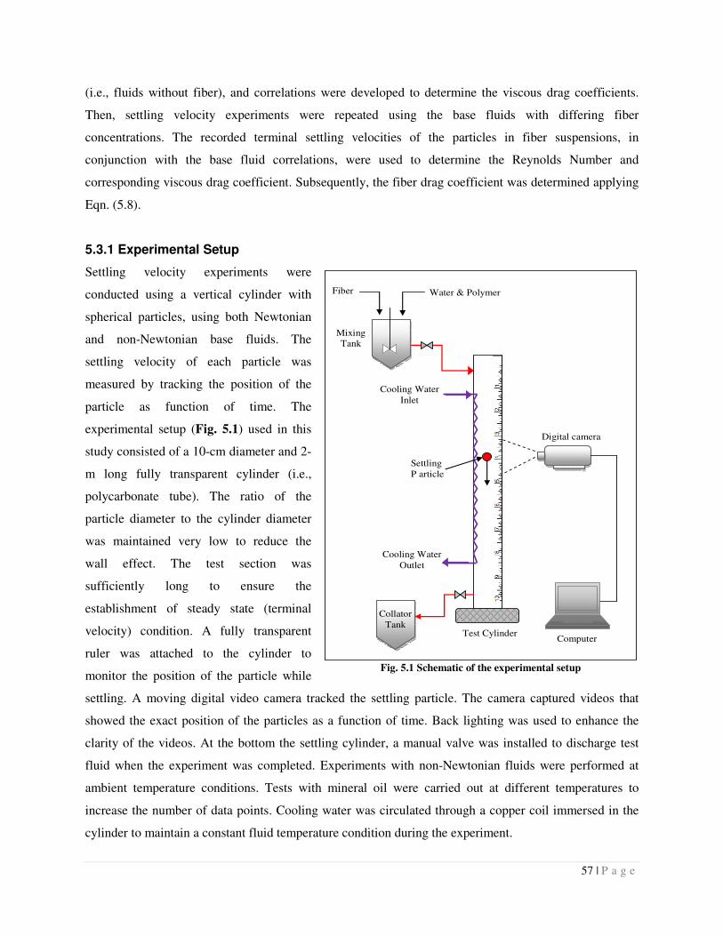
57 | P a g e

(i.e., fluids without fiber), and correlations were developed to determine the viscous drag coefficients.

Then, settling velocity experiments were repeated using the base fluids with differing fiber

concentrations. The recorded terminal settling velocities of the particles in fiber suspensions, in

conjunction with the base fluid correlations, were used to determine the Reynolds Number and

corresponding viscous drag coefficient. Subsequently, the fiber drag coefficient was determined applying

Eqn. (5.8).

5.3.1 Experimental Setup

Settling velocity experiments were

conducted using a vertical cylinder with

spherical particles, using both Newtonian

and non-Newtonian base fluids. The

settling velocity of each particle was

measured by tracking the position of the

particle as function of time. The

experimental setup (Fig. 5.1) used in this

study consisted of a 10-cm diameter and 2-

m long fully transparent cylinder (i.e.,

polycarbonate tube). The ratio of the

particle diameter to the cylinder diameter

was maintained very low to reduce the

wall effect. The test section was

sufficiently long to ensure the

establishment of steady state (terminal

velocity) condition. A fully transparent

ruler was attached to the cylinder to

monitor the position of the particle while

settling. A moving digital video camera tracked the settling particle. The camera captured videos that

showed the exact position of the particles as a function of time. Back lighting was used to enhance the

clarity of the videos. At the bottom the settling cylinder, a manual valve was installed to discharge test

fluid when the experiment was completed. Experiments with non-Newtonian fluids were performed at

ambient temperature conditions. Tests with mineral oil were carried out at different temperatures to

increase the number of data points. Cooling water was circulated through a copper coil immersed in the

cylinder to maintain a constant fluid temperature condition during the experiment.

Fig. 5.1 Schematic of the experimental setup

Mixing Tank

Test Cylinder

Digital camera

Computer

Collator Tank

Cooling Water Inlet

Cooling Water Outlet

Fiber Water & Polymer

Settling P article

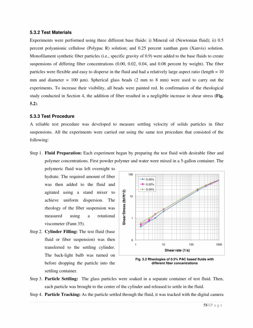
58 | P a g e

5.3.2 Test Materials

Experiments were performed using three different base fluids: i) Mineral oil (Newtonian fluid); ii) 0.5

percent polyanionic cellulose (Polypac R) solution; and 0.25 percent xanthan gum (Xanvis) solution.

Monofilament synthetic fiber particles (i.e., specific gravity of 0.9) were added to the base fluids to create

suspensions of differing fiber concentrations (0.00, 0.02, 0.04, and 0.08 percent by weight). The fiber

particles were flexible and easy to disperse in the fluid and had a relatively large aspect ratio (length = 10

mm and diameter = 100 µm). Spherical glass beads (2 mm to 8 mm) were used to carry out the

experiments. To increase their visibility, all beads were painted red. In confirmation of the rheological

study conducted in Section 4, the addition of fiber resulted in a negligible increase in shear stress (Fig.

5.2).

5.3.3 Test Procedure

A reliable test procedure was developed to measure settling velocity of solids particles in fiber

suspensions. All the experiments were carried out using the same test procedure that consisted of the

following:

Step 1. Fluid Preparation: Each experiment began by preparing the test fluid with desirable fiber and

polymer concentrations. First powder polymer and water were mixed in a 5-gallon container. The

polymeric fluid was left overnight to

hydrate. The required amount of fiber

was then added to the fluid and

agitated using a stand mixer to

achieve uniform dispersion. The

rheology of the fiber suspension was

measured using a rotational

viscometer (Fann 35).

Step 2. Cylinder Filling: The test fluid (base

fluid or fiber suspension) was then

transferred to the settling cylinder.

The back-light bulb was turned on

before dropping the particle into the

settling container.

Step 3. Particle Settling: The glass particles were soaked in a separate container of test fluid. Then,

each particle was brought to the center of the cylinder and released to settle in the fluid.

Step 4. Particle Tracking: As the particle settled through the fluid, it was tracked with the digital camera

Fig. 5.2 Rheologies of 0.5% PAC based fluids with different fiber concentrations

0

1

10

100

1 10 100 1000

Sh

ea

r S

tre

ss (

lbf/

ft^

2)

Shear rate (1/s)

0.00%

0.02%

0.04%

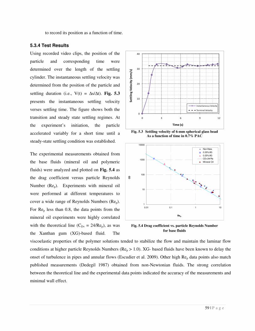
59 | P a g e

to record its position as a function of time.

5.3.4 Test Results

Using recorded video clips, the position of the

particle and corresponding time were

determined over the length of the settling

cylinder. The instantaneous settling velocity was

determined from the position of the particle and

settling duration (i.e., V(t) = ∆s/∆t). Fig. 5.3

presents the instantaneous settling velocity

verses settling time. The figure shows both the

transition and steady state settling regimes. At

the experiment’s initiation, the particle

accelerated variably for a short time until a

steady-state settling condition was established.

The experimental measurements obtained from

the base fluids (mineral oil and polymeric

fluids) were analyzed and plotted on Fig. 5.4 as

the drag coefficient versus particle Reynolds

Number (Rep). Experiments with mineral oil

were performed at different temperatures to

cover a wide range of Reynolds Numbers (Rep).

For Rep less than 0.8, the data points from the

mineral oil experiments were highly correlated

with the theoretical line (CDv = 24/Rep), as was

the Xanthan gum (XG)-based fluid. The

viscoelastic properties of the polymer solutions tended to stabilize the flow and maintain the laminar flow

conditions at higher particle Reynolds Numbers (Rep > 1.0). XG- based fluids have been known to delay the

onset of turbulence in pipes and annular flows (Escudier et al. 2009). Other high Rep data points also match

published measurements (Dedegil 1987) obtained from non-Newtonian fluids. The strong correlation

between the theoretical line and the experimental data points indicated the accuracy of the measurements and

minimal wall effect.

Fig. 5.3 Settling velocity of 6-mm spherical glass bead

As a function of time in 0.7% PAC

Fig. 5.4 Drag coefficient vs. particle Reynolds Number

for base fluids

0

10

20

30

40

0 3 6 9 12

Se

ttli

ng

Ve

loci

ty (

mm

/s)

Time (s)

Instantaneous Velocity

Terminal Velocity

1

10

100

1000

10000

0.01 0.1 1 10

Rep

CD

Non-New.

0.35%XG

0.25%XG

CD=24/Re

Mineral Oil

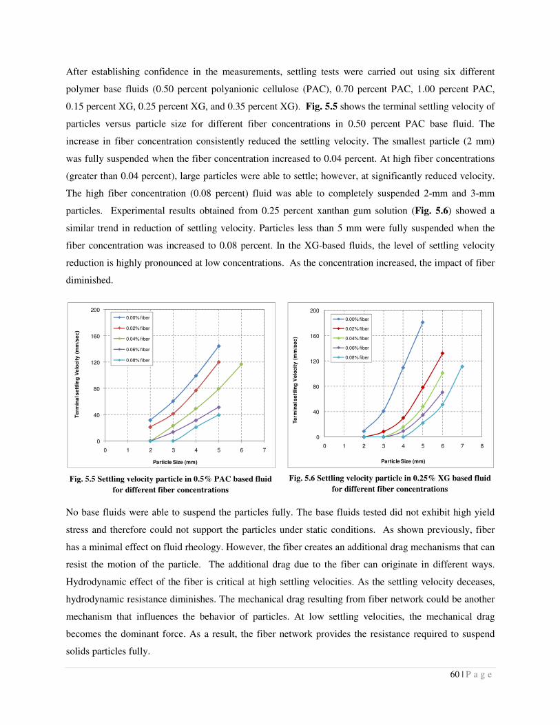
60 | P a g e

After establishing confidence in the measurements, settling tests were carried out using six different

polymer base fluids (0.50 percent polyanionic cellulose (PAC), 0.70 percent PAC, 1.00 percent PAC,

0.15 percent XG, 0.25 percent XG, and 0.35 percent XG). Fig. 5.5 shows the terminal settling velocity of

particles versus particle size for different fiber concentrations in 0.50 percent PAC base fluid. The

increase in fiber concentration consistently reduced the settling velocity. The smallest particle (2 mm)

was fully suspended when the fiber concentration increased to 0.04 percent. At high fiber concentrations

(greater than 0.04 percent), large particles were able to settle; however, at significantly reduced velocity.

The high fiber concentration (0.08 percent) fluid was able to completely suspended 2-mm and 3-mm

particles. Experimental results obtained from 0.25 percent xanthan gum solution (Fig. 5.6) showed a

similar trend in reduction of settling velocity. Particles less than 5 mm were fully suspended when the

fiber concentration was increased to 0.08 percent. In the XG-based fluids, the level of settling velocity

reduction is highly pronounced at low concentrations. As the concentration increased, the impact of fiber

diminished.

Fig. 5.5 Settling velocity particle in 0.5% PAC based fluid

for different fiber concentrations

Fig. 5.6 Settling velocity particle in 0.25% XG based fluid

for different fiber concentrations

No base fluids were able to suspend the particles fully. The base fluids tested did not exhibit high yield

stress and therefore could not support the particles under static conditions. As shown previously, fiber

has a minimal effect on fluid rheology. However, the fiber creates an additional drag mechanisms that can

resist the motion of the particle. The additional drag due to the fiber can originate in different ways.

Hydrodynamic effect of the fiber is critical at high settling velocities. As the settling velocity deceases,

hydrodynamic resistance diminishes. The mechanical drag resulting from fiber network could be another

mechanism that influences the behavior of particles. At low settling velocities, the mechanical drag

becomes the dominant force. As a result, the fiber network provides the resistance required to suspend

solids particles fully.

0

40

80

120

160

200

0 1 2 3 4 5 6 7

Te

rmin

al s

ett

lin

g V

elo

cit

y (

mm

/se

c)

Particle Size (mm)

0.00% fiber

0.02% fiber

0.04% fiber

0.06% fiber

0.08% fiber

0

40

80

120

160

200

0 1 2 3 4 5 6 7 8

Te

rmin

al s

ett

lin

g V

elo

cit

y (

mm

/se

c)

Particle Size (mm)

0.00% fiber

0.02% fiber

0.04% fiber

0.06% fiber

0.08% fiber

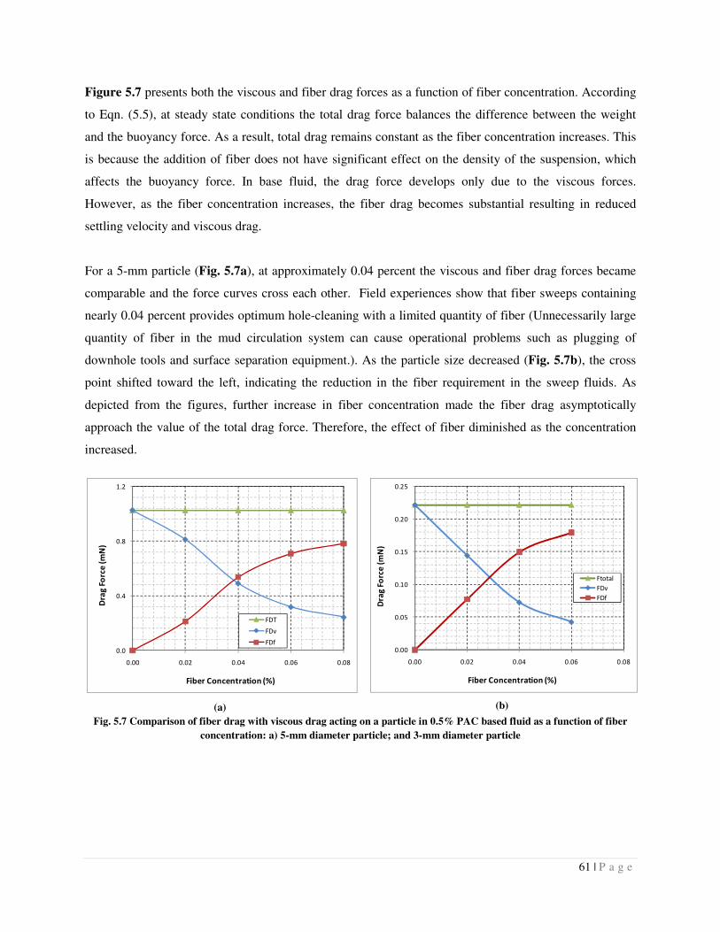
61 | P a g e

Figure 5.7 presents both the viscous and fiber drag forces as a function of fiber concentration. According

to Eqn. (5.5), at steady state conditions the total drag force balances the difference between the weight

and the buoyancy force. As a result, total drag remains constant as the fiber concentration increases. This

is because the addition of fiber does not have significant effect on the density of the suspension, which

affects the buoyancy force. In base fluid, the drag force develops only due to the viscous forces.

However, as the fiber concentration increases, the fiber drag becomes substantial resulting in reduced

settling velocity and viscous drag.

For a 5-mm particle (Fig. 5.7a), at approximately 0.04 percent the viscous and fiber drag forces became

comparable and the force curves cross each other. Field experiences show that fiber sweeps containing

nearly 0.04 percent provides optimum hole-cleaning with a limited quantity of fiber (Unnecessarily large

quantity of fiber in the mud circulation system can cause operational problems such as plugging of

downhole tools and surface separation equipment.). As the particle size decreased (Fig. 5.7b), the cross

point shifted toward the left, indicating the reduction in the fiber requirement in the sweep fluids. As

depicted from the figures, further increase in fiber concentration made the fiber drag asymptotically

approach the value of the total drag force. Therefore, the effect of fiber diminished as the concentration

increased.

(a)

(b)

Fig. 5.7 Comparison of fiber drag with viscous drag acting on a particle in 0.5% PAC based fluid as a function of fiber

concentration: a) 5-mm diameter particle; and 3-mm diameter particle

0.0

0.4

0.8

1.2

0.00 0.02 0.04 0.06 0.08

Dra

g F

orc

e (

mN

)

Fiber Concentration (%)

FDT

FDv

FDf0.00

0.05

0.10

0.15

0.20

0.25

0.00 0.02 0.04 0.06 0.08

Dra

g F

orc

e (

mN

)

Fiber Concentration (%)

Ftotal

FDv

FDf

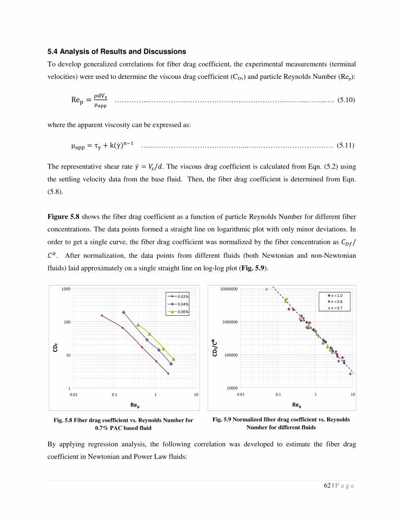
62 | P a g e

5.4 Analysis of Results and Discussions

To develop generalized correlations for fiber drag coefficient, the experimental measurements (terminal

velocities) were used to determine the viscous drag coefficient (CDv) and particle Reynolds Number (Rep):

Re� ��%:;�� …………...………………………………………………………...……..…. (5.10)

where the apparent viscosity can be expressed as:

μ=�� τ? @ kBγ� D�� …...………………………………...……………………………… (5.11)

The representative shear rate �� EF/H. The viscous drag coefficient is calculated from Eqn. (5.2) using

the settling velocity data from the base fluid. Then, the fiber drag coefficient is determined from Eqn.

(5.8).

Figure 5.8 shows the fiber drag coefficient as a function of particle Reynolds Number for different fiber

concentrations. The data points formed a straight line on logarithmic plot with only minor deviations. In

order to get a single curve, the fiber drag coefficient was normalized by the fiber concentration as IJK/IL. After normalization, the data points from different fluids (both Newtonian and non-Newtonian

fluids) laid approximately on a single straight line on log-log plot (Fig. 5.9).

Fig. 5.8 Fiber drag coefficient vs. Reynolds Number for

0.7% PAC based fluid

Fig. 5.9 Normalized fiber drag coefficient vs. Reynolds

Number for different fluids

By applying regression analysis, the following correlation was developed to estimate the fiber drag

coefficient in Newtonian and Power Law fluids:

1

10

100

1000

0.01 0.1 1 10

Rep

CD

f

0.02%

0.04%

0.06%

10000

100000

1000000

10000000

0.01 0.1 1 10

Rep

CD

f/C

αα αα

n = 1.0

n = 0.8

n = 0.7

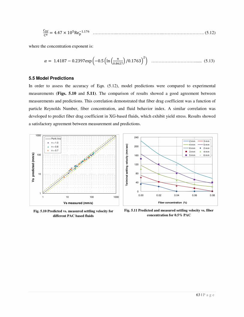
63 | P a g e

��M 4.47 Q 10SRe��.�TU ……………..…………………………..………………………. (5.12)

where the concentration exponent is:

V 1.4187 � 0.2397exp /�0.5 6ln 6 �`.aU�T7 /0.17637�2 …………………………...... (5.13)

5.5 Model Predictions

In order to assess the accuracy of Eqn. (5.12), model predictions were compared to experimental

measurements (Figs. 5.10 and 5.11). The comparison of results showed a good agreement between

measurements and predictions. This correlation demonstrated that fiber drag coefficient was a function of

particle Reynolds Number, fiber concentration, and fluid behavior index. A similar correlation was

developed to predict fiber drag coefficient in XG-based fluids, which exhibit yield stress. Results showed

a satisfactory agreement between measurement and predictions.

Fig. 5.10 Predicted vs. measured settling velocity for

different PAC based fluids

Fig. 5.11 Predicted and measured settling velocity vs. fiber

concentration for 0.5% PAC

1

10

100

1000

1 10 100 1000

Vs measured (mm/s)

Vs p

red

icte

d (m

m/s

)

Perfc line

n = 1.0

n = 0.8

n = 0.7

0

40

80

120

160

200

240

0.00 0.02 0.04 0.06 0.08

Teri

min

al sett

lin

g v

elo

cit

y (

mm

/sec)

Fiber concentration (%)

2 mm 3 mm

4 mm 5 mm

6 mm 2 mm

3 mm 4 mm

5 mm 6 mm

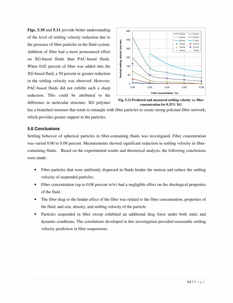
64 | P a g e

Figs. 5.10 and 5.11 provide better understanding

of the level of settling velocity reduction due to

the presence of fiber particles in the fluid system.

Addition of fiber had a more pronounced effect

on XG-based fluids than PAC-based fluids.

When 0.02 percent of fiber was added into the

XG-based fluid, a 50 percent or greater reduction

in the settling velocity was observed. However,

PAC-based fluids did not exhibit such a sharp

reduction. This could be attributed to the

difference in molecular structure. XG polymer

has a branched structure that tends to entangle with fiber particles to create strong polymer-fiber network,

which provides greater support to the particles.

5.6 Conclusions

Settling behavior of spherical particles in fiber-containing fluids was investigated. Fiber concentration

was varied 0.00 to 0.08 percent. Measurements showed significant reduction in settling velocity in fiber-

containing fluids. Based on the experimental results and theoretical analysis, the following conclusions

were made:

• Fiber particles that were uniformly dispersed in fluids hinder the motion and reduce the settling

velocity of suspended particles.

• Fiber concentration (up to 0.08 percent w/w) had a negligible effect on the rheological properties

of the fluid.

• The fiber drag or the hinder effect of the fiber was related to the fiber concentration, properties of

the fluid, and size, density, and settling velocity of the particle.

• Particles suspended in fiber sweep exhibited an additional drag force under both static and

dynamic conditions. The correlations developed in this investigation provided reasonable settling

velocity prediction in fiber suspensions.

Fig. 5.12 Predicted and measured settling velocity vs. fiber

concentration for 0.25% XG

0

80

160

240

320

400

480

0.00 0.02 0.04 0.06 0.08

Term

inal sett

lin

g v

elo

cit

y (

mm

/sec)

Fiber concentration (%)

2 mm 3 mm

4 mm 5 mm

6 mm 7 mm

2 mm 3 mm

4 mm 5 mm

6 mm 7 mm

65 | P a g e

Nomenclature

AP = projection area of a particle

CDv = Viscous drag coefficient

CDf = Fiber drag coefficient

d = diameter of a particle

FB = Buoyancy force

FD = Drag force

FDf = Fiber drag force

FDT = Total drag force

FDv = Viscous drag force

Fg = Gravitational force



m = Mass of a solids particle

NRep = Reynolds Number

n = fluid behavior index

Re = Reynolds Number

ReP = Particle Reynolds Number

t = Time

V = Instantaneous settling velocity of a particle

Vs = Terminal settling velocity of a particle

Greek Letters �� = Shear rate


µapp = Apparent fluid viscosity

ρf = Fluid density

ρp = Density of a particle

τy = yield stress

References

Ahmed, R.M. and Takach, N.E., 2008. Fiber Sweeps for Hole Cleaning. Paper SPE 113746 presented at

the SPE/ICoTA Coiled Tubing and Well Intervention Conference and Exhibition, The

Woodlands, Texas, 1-2 April.

Bivins. C.H., Bomey, CV., Fredd, C., Lassek, J., Sullivan, P., Engels, J., Fielder, E. O., Gorham, T.,

Judd, T., Mogollon, A E.S., Tabor, L., Munoz, A., and Willberg, D., 2005. New fibers for

hydraulic fracturing. Oilfield Review, Vol. 17, Issue 2, Schlumberger.

Baldock, T.E., Tomkins, M.R., Nielsen, P., Hughes, M.G., 2004. Settling velocity of sediments at high

concentrations. Coastal Eng. 51, 91-100.

Bulgachev, R.V. and Pouget, P., 2006., New Experience in Monofilament Fiber Tandem Sweeps Hole

Cleaning Performance on Kharyaga Oilfield, Timan-Pechora Region of Russia. Paper SPE

101961, presented at the SPE Russian Oil and Gas Technical Conference and Exhibition,

Moscow, 3–6 October. doi: 10.2118/101961-MS.

Cameron, C., Helmy, H., and Haikal, M. 2003., Fibrous LCM Sweeps Enhance Hole Cleaning and ROP

on Extended Reach Well in Abu Dhabi. Paper SPE 81419 presented at the Middle East Oil Show,

Bahrain, 9–12 June. doi: 10.2118/81419-MS.

66 | P a g e

Chhabra, R.P. and Peri, S.S. 1991., A simple method for the estimation of free fall velocity of spherical

particles in Power Law liquids. Powder Technology 67 (1991), pp. 287–290.

Chhabra, R. P. 2007., Bubbles, drops, and particles in non-Newtonian fluids, Second Edition, Taylor and

Francis Group, CRC Press, Florida.

Chhabra, R.P., 1980. Ph.D. Thesis, Monash University, Melbourne, Australia.

Chhabra. R.P., Agarwal. S. and Chaudhary. K., 2003. A note on wall effect on the terminal falling

velocity of a sphere in quiescent Newtonian media in cylindrical tube. Powder Technology, 129,

53-58.

Chien. S.F., 1994. Settling velocity of irregularly shaped particles, SPE Drilling & Completion, Vol. 9,

Num. 4, 281-289.

Dallon, D.S., 1967. A drag coefficient correlation for spheres settling in Ellis fluids. PhD Thesis,

University of Utah, Salt Lake City, UT.

Daneshy, A.A., 1978. Numerical Solution of Sand Transport in Hydraulic Fracturing. Journal of

Petroleum Technology, Vol. 30, Number 1, 132-140.

Dedegil, M.Y., 1987. Drag coefficient and settling velocity of particles in non-Newtonian suspensions.

Journal of fluids engineering, vol. 109/319.

De Felice, R., 1996. A relationship for the wall effect on the settling velocity of sphere at any flow

regime. Int. J. Multiphase Flow, vol. 22, No.3, 527-533.

Govier, G.W. and Aziz. K., 1972. The flow of complex mixtures in pipes, Second Edition, Krieger Pub

Co., Malabar, Florida.

George, M., Ahmed, R. and Growcock, F., 2011. Rheological Properties of Fiber-Containing Drilling

Sweeps at Ambient and High Temperature Conditions. Paper AADE-11-NTCE-35, presented at

the 2011 AADE National Technical Conference and Exhibition, Houston, April 12-14.

Harlen, O.G., Sundararajakumar, R.R., Koch. D.L., 1999. Numerical simulations of a sphere settling

through a suspension of neutrally buoyant fibers. J. fluid mech., vol. 388, pp. 355-388.

Hemphill, T. and Rojas, J.C., 2002. Exploration Drilling Fluid Sweeps: Their Evaluation, Timing, and

Applications. Paper SPE 77448 presented at the SPE Annual Technical Conference and

Exhibition, San Antonio, Texas, USA, 29 September–2 October. doi: 10.2118/77448-MS.

Highgate, D.J. and Whorlow, R.W., 1967. The viscous resistance to motion of a sphere falling through a

sheared non-Newtonian liquid. J. Appl. Phys. 18 1019.

Holzer, A. and Sommerfeld, M., 2008. New simple correlation formula for the drag coefficient of non-

spherical particle, Powder Technology, Vol. 184, Issue 3, 361-365.

Jin, L. and Penny, G.S., 1995. Dimensionless methods for study of particle settling in Non-Newtonian

fluids. Journal of Petroleum Technology, Vol. 47, Num. 3, 223-228.

67 | P a g e

Kelessidis. V.C., 2004. An explicit equation for the terminal velocity of solid spheres falling in

pesudoplastic liquid, Chem. Eng. 59, 4435-4445.

Lali, A.M., Khare, A.S. and Joshi, J.B., 1988. Behavior of solid particles in viscous Non-Newtonian

solutions: settling velocity, wall effect and bed expansion in solid-liquid fluidized beds. Powder

Technology, 57, 39-50.

Marti, I., Höfler,O., Fischer P. and Windhab, E.J., 2005 Rheology of concentrated suspensions containing

mixtures of spheres and fibres, Rheol Acta, 44: 502–512

Prakash, S., 1983. Experimental evaluation of terminal velocity in non-Newtonian fluids in the turbulent

region, Ind. Chem. Eng. 25 (1983), pp. 1–4.

Phani, B.G., Yajun, L., Jay, N., Roger, B. and Mukul, M.S., 2004. Modeling proppant settling in water-

Fracs, paper SPE 89875, presented at the SPE Annual Technical Conference and Exhibition, 26-

29 September, Houston, Texas.

Rajabian, M., Dubois, C., Grmela, M. and Carreau, P.J., 2008. Effects of polymer–fiber interactions on

rheology and flow behavior of suspensions of semi-flexible fibers in polymeric liquids. Rheol

Acta 47:701–717.

Sadowski.Z., Mager. J. and Laskowski. J. 1978., Hindered settling of coagulating suspensions. Powder

Technology, Vol. 21, Issue 1, 73-79.

Shah, S.N., El Fadili. Y. and Chhabra. R.P., 2007. New model for single spherical particle settling

velocity in power law (visco-inelastic) fluids. Int. J. multiphase flow. 33, 51-66.

Shah, S.N., 1982. Proppant settling correlations for Non-Newtonian fluids under static and dynamic

conditions. SPE Journal, Vol. 22, Num. 2, 164-170.

Smith, T.N., 1998. A model of settling velocity. Chemical Eng. Science, Vol. 53, Issue 2, 315-323.

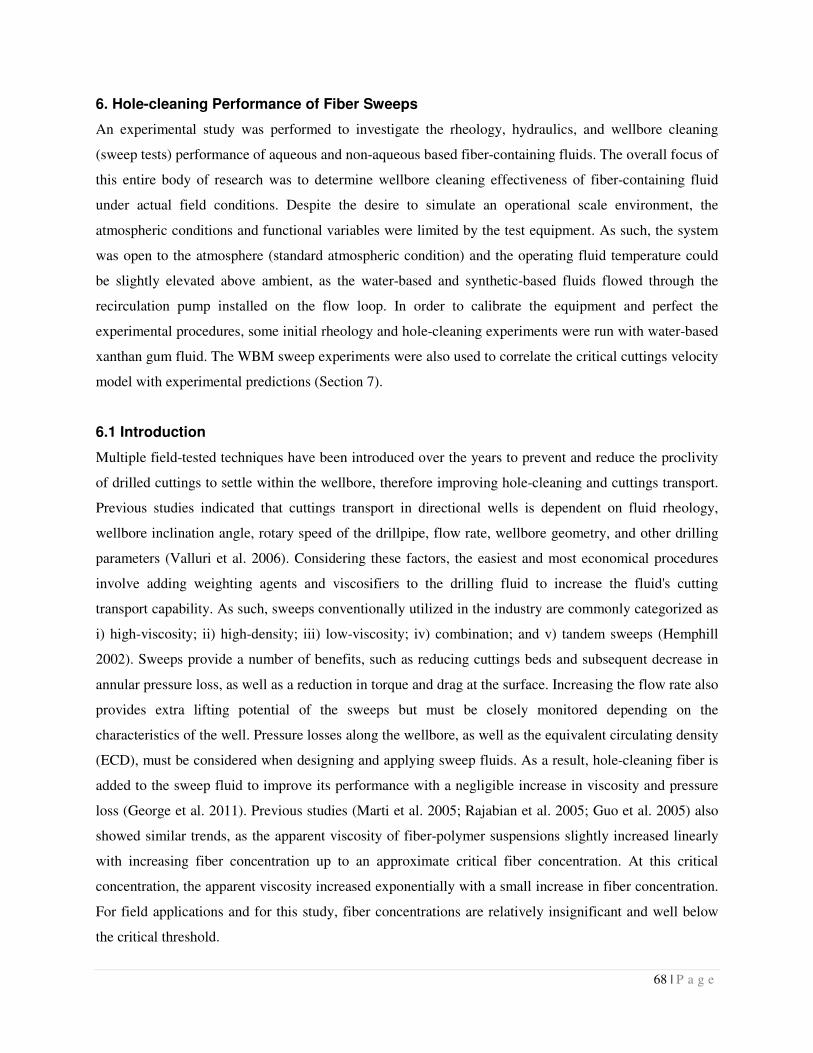
68 | P a g e

6. Hole-cleaning Performance of Fiber Sweeps

An experimental study was performed to investigate the rheology, hydraulics, and wellbore cleaning

(sweep tests) performance of aqueous and non-aqueous based fiber-containing fluids. The overall focus of

this entire body of research was to determine wellbore cleaning effectiveness of fiber-containing fluid

under actual field conditions. Despite the desire to simulate an operational scale environment, the

atmospheric conditions and functional variables were limited by the test equipment. As such, the system

was open to the atmosphere (standard atmospheric condition) and the operating fluid temperature could

be slightly elevated above ambient, as the water-based and synthetic-based fluids flowed through the

recirculation pump installed on the flow loop. In order to calibrate the equipment and perfect the

experimental procedures, some initial rheology and hole-cleaning experiments were run with water-based

xanthan gum fluid. The WBM sweep experiments were also used to correlate the critical cuttings velocity

model with experimental predictions (Section 7).

6.1 Introduction

Multiple field-tested techniques have been introduced over the years to prevent and reduce the proclivity

of drilled cuttings to settle within the wellbore, therefore improving hole-cleaning and cuttings transport.

Previous studies indicated that cuttings transport in directional wells is dependent on fluid rheology,

wellbore inclination angle, rotary speed of the drillpipe, flow rate, wellbore geometry, and other drilling

parameters (Valluri et al. 2006). Considering these factors, the easiest and most economical procedures

involve adding weighting agents and viscosifiers to the drilling fluid to increase the fluid's cutting

transport capability. As such, sweeps conventionally utilized in the industry are commonly categorized as

i) high-viscosity; ii) high-density; iii) low-viscosity; iv) combination; and v) tandem sweeps (Hemphill

2002). Sweeps provide a number of benefits, such as reducing cuttings beds and subsequent decrease in

annular pressure loss, as well as a reduction in torque and drag at the surface. Increasing the flow rate also

provides extra lifting potential of the sweeps but must be closely monitored depending on the

characteristics of the well. Pressure losses along the wellbore, as well as the equivalent circulating density

(ECD), must be considered when designing and applying sweep fluids. As a result, hole-cleaning fiber is

added to the sweep fluid to improve its performance with a negligible increase in viscosity and pressure

loss (George et al. 2011). Previous studies (Marti et al. 2005; Rajabian et al. 2005; Guo et al. 2005) also

showed similar trends, as the apparent viscosity of fiber-polymer suspensions slightly increased linearly

with increasing fiber concentration up to an approximate critical fiber concentration. At this critical

concentration, the apparent viscosity increased exponentially with a small increase in fiber concentration.

For field applications and for this study, fiber concentrations are relatively insignificant and well below

the critical threshold.

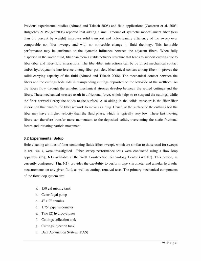
69 | P a g e

Previous experimental studies (Ahmed and Takach 2008) and field applications (Cameron et al. 2003;

Bulgachev & Pouget 2006) reported that adding a small amount of synthetic monofilament fiber (less

than 0.1 percent by weight) improves solid transport and hole-cleaning efficiency of the sweep over

comparable non-fiber sweeps, and with no noticeable change in fluid rheology. This favorable

performance may be attributed to the dynamic influence between the adjacent fibers. When fully

dispersed in the sweep fluid, fiber can form a stable network structure that tends to support cuttings due to

fiber-fiber and fiber-fluid interactions. The fiber-fiber interactions can be by direct mechanical contact

and/or hydrodynamic interference among fiber particles. Mechanical contact among fibers improves the

solids-carrying capacity of the fluid (Ahmed and Takach 2008). The mechanical contact between the

fibers and the cuttings beds aids in resuspending cuttings deposited on the low-side of the wellbore. As

the fibers flow through the annulus, mechanical stresses develop between the settled cuttings and the

fibers. These mechanical stresses result in a frictional force, which helps to re-suspend the cuttings, while

the fiber networks carry the solids to the surface. Also aiding in the solids transport is the fiber-fiber

interaction that enables the fiber network to move as a plug. Hence, at the surface of the cuttings bed the

fiber may have a higher velocity than the fluid phase, which is typically very low. These fast moving

fibers can therefore transfer more momentum to the deposited solids, overcoming the static frictional

forces and initiating particle movement.

6.2 Experimental Setup

Hole-cleaning abilities of fiber-containing fluids (fiber sweep), which are similar to those used for sweeps

in real wells, were investigated. Fiber sweep performance tests were conducted using a flow loop

apparatus (Fig. 6.1) available at the Well Construction Technology Center (WCTC). This device, as

currently configured (Fig. 6.2), provides the capability to perform pipe viscometer and annular hydraulic

measurements on any given fluid, as well as cuttings removal tests. The primary mechanical components

of the flow loop system are:

a. 150 gal mixing tank

b. Centrifugal pump

c. 4” x 2” annulus

d. 1.75” pipe viscometer

e. Two (2) hydrocyclones

f. Cuttings collection tank

g. Cuttings injection tank

h. Data Acquisition System (DAS)

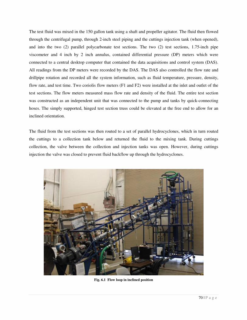
70 | P a g e

The test fluid was mixed in the 150 gallon tank using a shaft and propeller agitator. The fluid then flowed

through the centrifugal pump, through 2-inch steel piping and the cuttings injection tank (when opened),

and into the two (2) parallel polycarbonate test sections. The two (2) test sections, 1.75-inch pipe

viscometer and 4 inch by 2 inch annulus, contained differential pressure (DP) meters which were

connected to a central desktop computer that contained the data acquisitions and control system (DAS).

All readings from the DP meters were recorded by the DAS. The DAS also controlled the flow rate and

drillpipe rotation and recorded all the system information, such as fluid temperature, pressure, density,

flow rate, and test time. Two coriolis flow meters (F1 and F2) were installed at the inlet and outlet of the

test sections. The flow meters measured mass flow rate and density of the fluid. The entire test section

was constructed as an independent unit that was connected to the pump and tanks by quick-connecting

hoses. The simply supported, hinged test section truss could be elevated at the free end to allow for an

inclined orientation.

The fluid from the test sections was then routed to a set of parallel hydrocyclones, which in turn routed

the cuttings to a collection tank below and returned the fluid to the mixing tank. During cuttings

collection, the valve between the collection and injection tanks was open. However, during cuttings

injection the valve was closed to prevent fluid backflow up through the hydrocyclones.

Fig. 6.1 Flow loop in inclined position

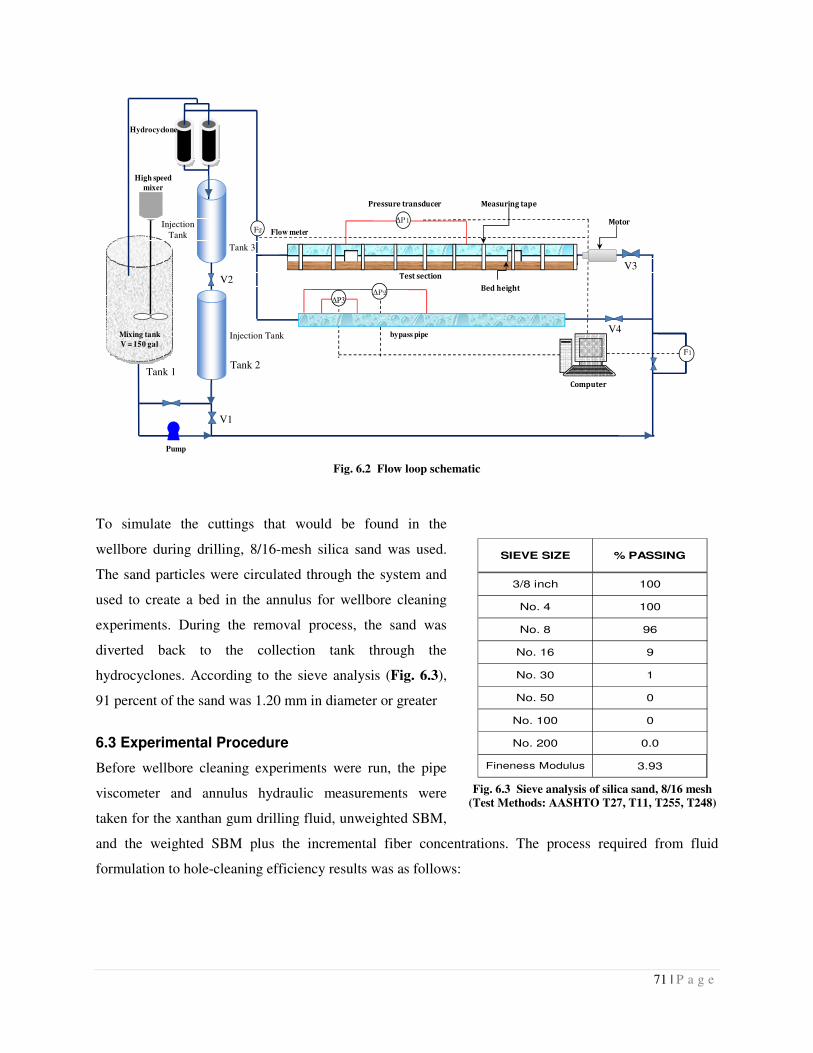
71 | P a g e

Fig. 6.2 Flow loop schematic

To simulate the cuttings that would be found in the

wellbore during drilling, 8/16-mesh silica sand was used.

The sand particles were circulated through the system and

used to create a bed in the annulus for wellbore cleaning

experiments. During the removal process, the sand was

diverted back to the collection tank through the

hydrocyclones. According to the sieve analysis (Fig. 6.3),

91 percent of the sand was 1.20 mm in diameter or greater

6.3 Experimental Procedure

Before wellbore cleaning experiments were run, the pipe

viscometer and annulus hydraulic measurements were

taken for the xanthan gum drilling fluid, unweighted SBM,

and the weighted SBM plus the incremental fiber concentrations. The process required from fluid

formulation to hole-cleaning efficiency results was as follows:

Fig. 6.3 Sieve analysis of silica sand, 8/16 mesh

(Test Methods: AASHTO T27, T11, T255, T248)

Fineness Modulus

No. 30

No. 8

3/8 inch

No. 4

No. 200 0.0

3.93

No. 50 0

No. 100 0

1

No. 16 9

96

100

100

SIEVE SIZE % PASSING

F1F1

∆P1

∆P2

F2

bypass pipe

Test section

Pump

Cutting Collection

or injection tank

Hydrocyclone

High speed

mixer

Mixing tank

V = 150 gal

Pressure transducer

Flow meter

∆P3

F1

Measuring tape

Computer

Bed height

Motor

Tank 1 Tank 2

Tank 3

Injection Tank

Injection Tank

V1

V2

V3

V4

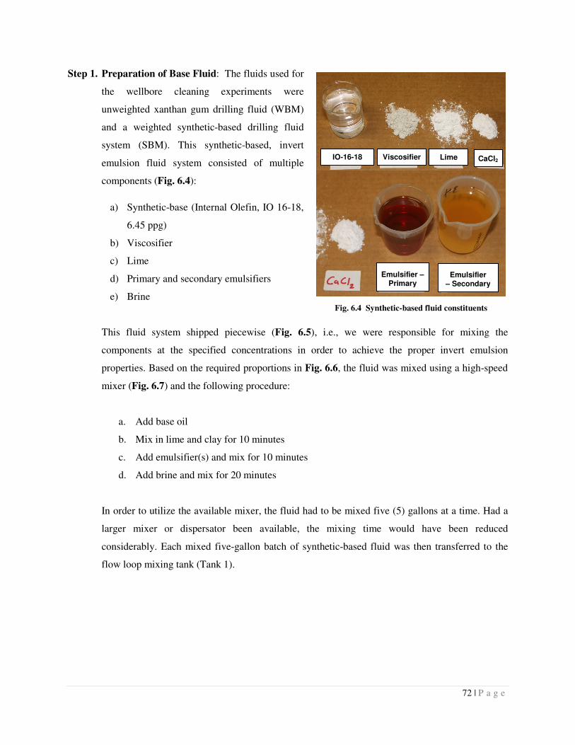
72 | P a g e

Step 1. Preparation of Base Fluid: The fluids used for

the wellbore cleaning experiments were

unweighted xanthan gum drilling fluid (WBM)

and a weighted synthetic-based drilling fluid

system (SBM). This synthetic-based, invert

emulsion fluid system consisted of multiple

components (Fig. 6.4):

a) Synthetic-base (Internal Olefin, IO 16-18,

6.45 ppg)

b) Viscosifier

c) Lime

d) Primary and secondary emulsifiers

e) Brine

This fluid system shipped piecewise (Fig. 6.5), i.e., we were responsible for mixing the

components at the specified concentrations in order to achieve the proper invert emulsion

properties. Based on the required proportions in Fig. 6.6, the fluid was mixed using a high-speed

mixer (Fig. 6.7) and the following procedure:

a. Add base oil

b. Mix in lime and clay for 10 minutes

c. Add emulsifier(s) and mix for 10 minutes

d. Add brine and mix for 20 minutes

In order to utilize the available mixer, the fluid had to be mixed five (5) gallons at a time. Had a

larger mixer or dispersator been available, the mixing time would have been reduced

considerably. Each mixed five-gallon batch of synthetic-based fluid was then transferred to the

flow loop mixing tank (Tank 1).

Fig. 6.4 Synthetic-based fluid constituents

Viscosifier Lime CaCl2

Emulsifier – Primary

IO-16-18

Emulsifier – Secondary

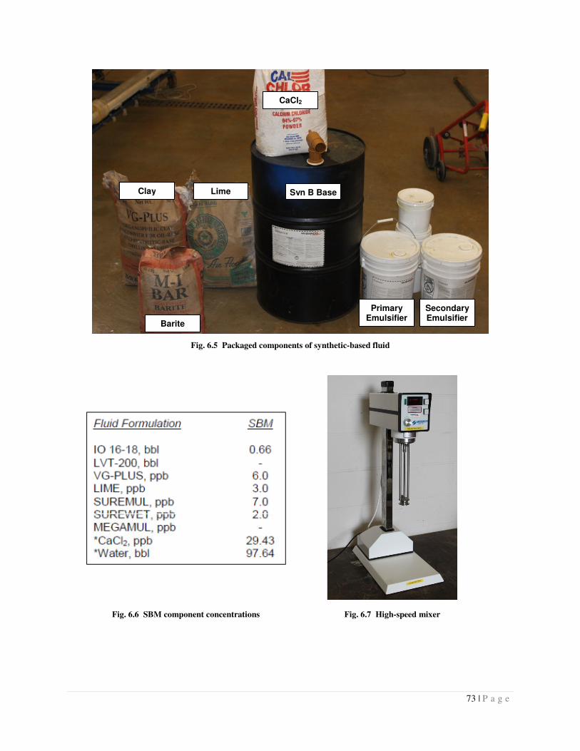
73 | P a g e

Fig. 6.5 Packaged components of synthetic-based fluid

Fig. 6.6 SBM component concentrations Fig. 6.7 High-speed mixer

Syn B Base

Primary Emulsifier

Secondary Emulsifier

Lime Clay

Barite

CaCl2

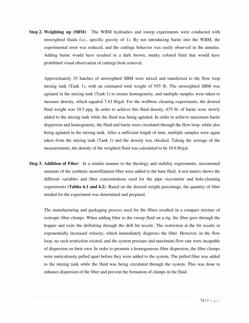
74 | P a g e

Step 2. Weighting up (SBM): The WBM hydraulics and sweep experiments were conducted with

unweighted fluids (i.e., specific gravity of 1). By not introducing barite into the WBM, the

experimental error was reduced, and the cuttings behavior was easily observed in the annulus.

Adding barite would have resulted in a dark brown, murky colored fluid that would have

prohibited visual observation of cuttings beds removal.

Approximately 35 batches of unweighted SBM were mixed and transferred to the flow loop

mixing tank (Tank 1), with an estimated total weight of 955 lb. The unweighted SBM was

agitated in the mixing tank (Tank 1) to ensure homogeneity, and multiple samples were taken to

measure density, which equaled 7.43 lb/gal. For the wellbore cleaning experiments, the desired

fluid weight was 10.5 ppg. In order to achieve this fluid density, 675 lb. of barite were slowly

added to the mixing tank while the fluid was being agitated. In order to achieve maximum barite

dispersion and homogeneity, the fluid and barite were circulated through the flow loop, while also

being agitated in the mixing tank. After a sufficient length of time, multiple samples were again

taken from the mixing tank (Tank 1) and the density was checked. Taking the average of the

measurements, the density of the weighted fluid was calculated to be 10.6 lb/gal.

Step 3. Addition of Fiber: In a similar manner to the rheology and stability experiments, incremental

amounts of the synthetic monofilament fiber were added to the base fluid. A test matrix shows the

different variables and fiber concentrations used for the pipe viscometer and hole-cleaning

experiments (Tables 6.1 and 6.2). Based on the desired weight percentage, the quantity of fiber

needed for the experiment was determined and prepared.

The manufacturing and packaging process used for the fibers resulted in a compact mixture of

isotropic fiber clumps. When adding fiber to the sweep fluid on a rig, the fiber goes through the

hopper and exits the drillstring through the drill bit nozzle. The restriction at the bit results in

exponentially increased velocity, which immediately disperses the fiber. However, in the flow

loop, no such restriction existed, and the system pressure and maximum flow rate were incapable

of dispersion on their own. In order to promote a homogeneous fiber dispersion, the fiber clumps

were meticulously pulled apart before they were added to the system. The pulled fiber was added

to the mixing tank while the fluid was being circulated through the system. This was done to

enhance dispersion of the fiber and prevent the formation of clumps in the fluid.

75 | P a g e

Step 4. Pipe Viscometer Measurements: The test fluid (base fluid and fiber) was first thoroughly

homogenized by circulating through the flow loop at a high flow rate until the fluid temperature

reached approximately 40°C due to viscous heating. Once the fluid increased to proper

temperature, the flow was diverted through the 1.75-inch pipe viscometer. Starting with a flow

rate of 10 gpm, the fluid was allowed to flow until the data acquisition system stabilized the flow

rate and a sufficient number of data points were recorded. The flow rate was then adjusted

accordingly.

Step 5. Cuttings Bed/Accumulation in Annulus: Once all pipe viscometer measurements were taken,

the flow was diverted back to the annulus. The valve (V1) below the cuttings injection tank (Tank

2) was then opened, while the valve (V2) between the collection tank (Tank 3) and injection tank

(Tank 2) was closed. The flow was again initiated at a medium rate (∼ 40 gpm) until cuttings

begin to appear in the annulus. The flow rate was then decreased (∼ 10 gpm) to allow the cuttings

to settle out of the fluid and form a bed on the low side of the annulus. This process was

continued until the cuttings bed was sufficiently deep and is no longer increasing in depth. For the

high-inertia, SBM this process took up to 30 - 45 minutes, since the cuttings did not easily settle

out of the high yield stress, plug flow zone.

Step 6. Flush Cuttings from System: Once the cuttings bed was established, the injection tank (Tank 2)

outlet valve (V1) was closed, and the middle valve (V2) was opened. Then the valve to the

annulus (V3) was closed while the pipe viscometer valve (V4) was opened. Once the valve

configurations were complete, the fluid was pumped through the system at a high flow rate to

clear the piping of any remaining cuttings. This process was continued until no cuttings were

observed in the transparent pipe viscometer, and until the density readings of the inlet and outlet

coriolis flow meters (F1 and F2) were approximately equivalent.

Step 7. Sweep Fluid Circulation/Cuttings Removal: Once the latent cuttings were flushed from the

system, the flow was stopped and the annulus and pipe viscometer valves were opened and

closed, respectively. Flow again was initiated at a low flow rate (10 gpm), with or without pipe

rotation, depending on the test matrix. The fluid was circulated through the annulus until the

density readings the coriolis meters at the entrance and exit of the annulus converged to within

0.015 g/cc.

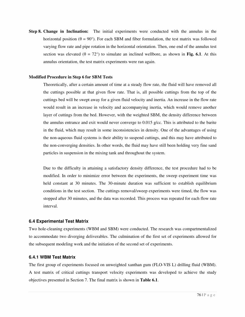
76 | P a g e

Step 8. Change in Inclination: The initial experiments were conducted with the annulus in the

horizontal position (θ = 90°). For each SBM and fiber formulation, the test matrix was followed

varying flow rate and pipe rotation in the horizontal orientation. Then, one end of the annulus test

section was elevated (θ = 72°) to simulate an inclined wellbore, as shown in Fig. 6.1. At this

annulus orientation, the test matrix experiments were ran again.

Modified Procedure in Step 6 for SBM Tests

Theoretically, after a certain amount of time at a steady flow rate, the fluid will have removed all

the cuttings possible at that given flow rate. That is, all possible cuttings from the top of the

cuttings bed will be swept away for a given fluid velocity and inertia. An increase in the flow rate

would result in an increase in velocity and accompanying inertia, which would remove another

layer of cuttings from the bed. However, with the weighted SBM, the density difference between

the annulus entrance and exit would never converge to 0.015 g/cc. This is attributed to the barite

in the fluid, which may result in some inconsistencies in density. One of the advantages of using

the non-aqueous fluid systems is their ability to suspend cuttings, and this may have attributed to

the non-converging densities. In other words, the fluid may have still been holding very fine sand

particles in suspension in the mixing tank and throughout the system.

Due to the difficulty in attaining a satisfactory density difference, the test procedure had to be

modified. In order to minimize error between the experiments, the sweep experiment time was

held constant at 30 minutes. The 30-minute duration was sufficient to establish equilibrium

conditions in the test section. The cuttings removal/sweep experiments were timed, the flow was

stopped after 30 minutes, and the data was recorded. This process was repeated for each flow rate

interval.

6.4 Experimental Test Matrix

Two hole-cleaning experiments (WBM and SBM) were conducted. The research was compartmentalized

to accommodate two diverging deliverables. The culmination of the first set of experiments allowed for

the subsequent modeling work and the initiation of the second set of experiments.

6.4.1 WBM Test Matrix

The first group of experiments focused on unweighted xanthan gum (FLO-VIS L) drilling fluid (WBM).

A test matrix of critical cuttings transport velocity experiments was developed to achieve the study

objectives presented in Section 7. The final matrix is shown in Table 6.1.

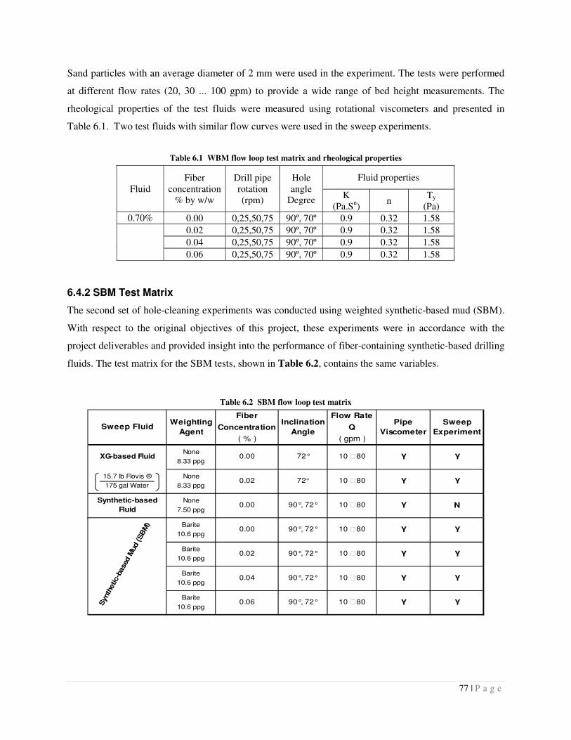
77 | P a g e

Sand particles with an average diameter of 2 mm were used in the experiment. The tests were performed

at different flow rates (20, 30 ... 100 gpm) to provide a wide range of bed height measurements. The

rheological properties of the test fluids were measured using rotational viscometers and presented in

Table 6.1. Two test fluids with similar flow curves were used in the sweep experiments.

Table 6.1 WBM flow loop test matrix and rheological properties

6.4.2 SBM Test Matrix

The second set of hole-cleaning experiments was conducted using weighted synthetic-based mud (SBM).

With respect to the original objectives of this project, these experiments were in accordance with the

project deliverables and provided insight into the performance of fiber-containing synthetic-based drilling

fluids. The test matrix for the SBM tests, shown in Table 6.2, contains the same variables.

Table 6.2 SBM flow loop test matrix

Fluid Fiber

concentration % by w/w

Drill pipe rotation (rpm)

Hole angle

Degree

Fluid properties

K (Pa.Sn)

n Ty

(Pa)

0.70% XG

0.00 0,25,50,75 90º, 70º 0.9 0.32 1.58

0.02 0,25,50,75 90º, 70º 0.9 0.32 1.58

0.04 0,25,50,75 90º, 70º 0.9 0.32 1.58

0.06 0,25,50,75 90º, 70º 0.9 0.32 1.58

Fiber Flow Rate

Concentration Q

( % ) ( gpm )

None

8.33 ppg

15.7 lb Flovis ® None

175 gal Water 8.33 ppg

None

7.50 ppg

Sweep Fluid

Synthetic-based

Fluid

XG-based Fluid

Synth

etic-b

ased

Mud (SB

M)

72°

72°

10 ‒ 80

10 ‒ 80

10 ‒ 80

10 ‒ 80

Weighting

Agent

Inclination

Angle

90°, 72°

Sweep

Experiment

Pipe

Viscometer

Y

Y

0.00

0.02

0.00

0.00

Y

Y

N

Y

Y

Y

90°, 72°

Barite

10.6 ppg

Barite

10.6 ppg

Barite

10.6 ppg

Barite

10.6 ppgSynth

etic-b

ased

Mud (SB

M)

10 ‒ 80

10 ‒ 80

10 ‒ 80

10 ‒ 80

90°, 72°

90°, 72°

90°, 72°

90°, 72°

0.06 Y

Y

Y

Y

Y

0.00

0.02

0.04

Y

Y

Y

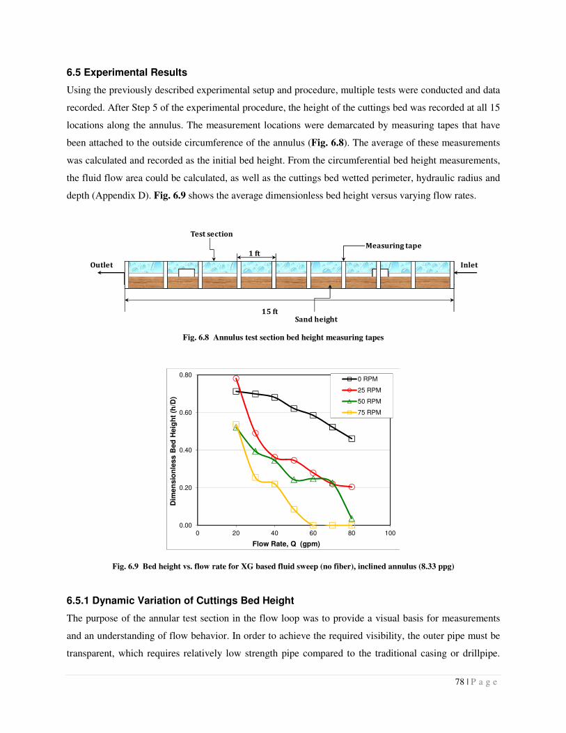
78 | P a g e


Using the previously described experimental setup and procedure, multiple tests were conducted and data

recorded. After Step 5 of the experimental procedure, the height of the cuttings bed was recorded at all 15

locations along the annulus. The measurement locations were demarcated by measuring tapes that have

been attached to the outside circumference of the annulus (Fig. 6.8). The average of these measurements

was calculated and recorded as the initial bed height. From the circumferential bed height measurements,

the fluid flow area could be calculated, as well as the cuttings bed wetted perimeter, hydraulic radius and

depth (Appendix D). Fig. 6.9 shows the average dimensionless bed height versus varying flow rates.

Fig. 6.8 Annulus test section bed height measuring tapes

Fig. 6.9 Bed height vs. flow rate for XG based fluid sweep (no fiber), inclined annulus (8.33 ppg)

6.5.1 Dynamic Variation of Cuttings Bed Height

The purpose of the annular test section in the flow loop was to provide a visual basis for measurements

and an understanding of flow behavior. In order to achieve the required visibility, the outer pipe must be

transparent, which requires relatively low strength pipe compared to the traditional casing or drillpipe.

Inlet Outlet

Measuring tape1 ft

15 ftSand height

Test section

0.00

0.20

0.40

0.60

0.80

0 20 40 60 80 100

Dim

en

sio

nle

ss

Bed

He

igh

t (h

/D)

Flow Rate, Q (gpm)

0 RPM

25 RPM

50 RPM

75 RPM

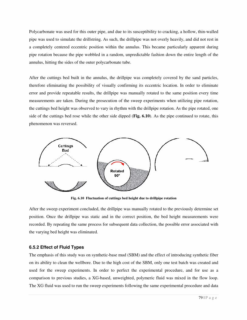
Polycarbonate was used for this outer pipe, and due to its susceptibility to cracking, a hollow, thin

pipe was used to simulate the drillstring. As such, the drillpipe

a completely centered eccentric position within the annulus. This

pipe rotation because the pipe wobble

annulus, hitting the sides of the outer polycarbonate tube.

After the cuttings bed built in the annulus, the drillpipe

therefore eliminating the possibility of visually confirming its eccentric location. In order to eliminate

error and provide repeatable results, the drillpipe

measurements are taken. During the prosecution of the sweep experiments when utilizing pipe rotation,

the cuttings bed height was observed to vary in rhythm wit

side of the cuttings bed rose while the other side dipped (

phenomenon was reversed.

Fig. 6.10 Fluctuation of cuttings bed height due to drillpipe

After the sweep experiment concluded, the drillpipe was manually rotated to the previously determine set

position. Once the drillpipe was static and in the correct position, the bed height measurements were

recorded. By repeating the same process for subsequent data collection, the possible error associated with

the varying bed height was eliminated.

6.5.2 Effect of Fluid Types

The emphasis of this study was on synthetic

on its ability to clean the wellbore. Due to the high cost of the SBM, only one test batch was created and

used for the sweep experiments. In order to perfect the experimental procedure, and for use as a

comparison to previous studies, a XG

The XG fluid was used to run the sweep experiments following the same experimental procedure and data

Polycarbonate was used for this outer pipe, and due to its susceptibility to cracking, a hollow, thin

pipe was used to simulate the drillstring. As such, the drillpipe was not overly heavily, and

a completely centered eccentric position within the annulus. This became particularly apparent during

wobbled in a random, unpredictable fashion down the entire length of the

of the outer polycarbonate tube.

After the cuttings bed built in the annulus, the drillpipe was completely covered by the sand particles,


provide repeatable results, the drillpipe was manually rotated to the same position every time


the cuttings bed height was observed to vary in rhythm with the drillpipe rotation. As the pipe rotated, one

side of the cuttings bed rose while the other side dipped (Fig. 6.10). As the pipe continued to rotate, this

Fig. 6.10 Fluctuation of cuttings bed height due to drillpipe rotation



process for subsequent data collection, the possible error associated with

the varying bed height was eliminated.

on synthetic-base mud (SBM) and the effect of introducing synthetic fiber

bility to clean the wellbore. Due to the high cost of the SBM, only one test batch was created and


comparison to previous studies, a XG-based, unweighted, polymeric fluid was mixed in the flow loop.


79 | P a g e

Polycarbonate was used for this outer pipe, and due to its susceptibility to cracking, a hollow, thin-walled

ly, and did not rest in

particularly apparent during

fashion down the entire length of the

completely covered by the sand particles,


manually rotated to the same position every time


h the drillpipe rotation. As the pipe rotated, one

). As the pipe continued to rotate, this



process for subsequent data collection, the possible error associated with

base mud (SBM) and the effect of introducing synthetic fiber

bility to clean the wellbore. Due to the high cost of the SBM, only one test batch was created and


meric fluid was mixed in the flow loop.


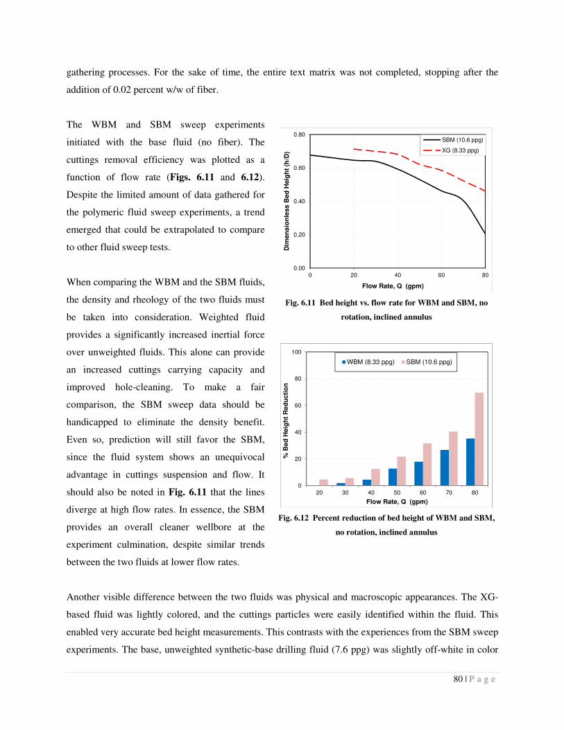
80 | P a g e

gathering processes. For the sake of time, the entire text matrix was not completed, stopping after the

addition of 0.02 percent w/w of fiber.

The WBM and SBM sweep experiments

initiated with the base fluid (no fiber). The

cuttings removal efficiency was plotted as a

function of flow rate (Figs. 6.11 and 6.12).

Despite the limited amount of data gathered for

the polymeric fluid sweep experiments, a trend

emerged that could be extrapolated to compare

to other fluid sweep tests.

When comparing the WBM and the SBM fluids,

the density and rheology of the two fluids must

be taken into consideration. Weighted fluid

provides a significantly increased inertial force

over unweighted fluids. This alone can provide

an increased cuttings carrying capacity and

improved hole-cleaning. To make a fair

comparison, the SBM sweep data should be

handicapped to eliminate the density benefit.

Even so, prediction will still favor the SBM,

since the fluid system shows an unequivocal

advantage in cuttings suspension and flow. It

should also be noted in Fig. 6.11 that the lines

diverge at high flow rates. In essence, the SBM

provides an overall cleaner wellbore at the

experiment culmination, despite similar trends

between the two fluids at lower flow rates.

Another visible difference between the two fluids was physical and macroscopic appearances. The XG-

based fluid was lightly colored, and the cuttings particles were easily identified within the fluid. This

enabled very accurate bed height measurements. This contrasts with the experiences from the SBM sweep

experiments. The base, unweighted synthetic-base drilling fluid (7.6 ppg) was slightly off-white in color

Fig. 6.11 Bed height vs. flow rate for WBM and SBM, no

rotation, inclined annulus

Fig. 6.12 Percent reduction of bed height of WBM and SBM,

no rotation, inclined annulus

0.00

0.20

0.40

0.60

0.80

0 20 40 60 80

Dim

en

sio

nle

ss

Be

d H

eig

ht

(h/D

)Flow Rate, Q (gpm)

SBM (10.6 ppg)

XG (8.33 ppg)

0

20

40

60

80

100

20 30 40 50 60 70 80

% B

ed

Heig

ht

Re

du

cti

on

Flow Rate, Q (gpm)

WBM (8.33 ppg) SBM (10.6 ppg)

81 | P a g e

and clean. Once barite was added to the system, the color changed to dark brown, and small barite clumps

could be seen floating in the fluid. This provided difficulty in precisely measuring the bed height because

the dark color of the fluid closely matched that of the cuttings particles. Therefore, bed height

measurements were taken based on the shaded areas of the annulus, present from the cuttings beds inside.

Individual cuttings particles could no longer be identified. Due to the density of the fluid and the particles

suspended within, the coriolis flow meters were constantly measuring relatively large differences in

density. The difference was apparent during rheology and hydraulics measurements, but it was

exacerbated during sweep experiments. The ability of the fluid to suspend the cuttings and the presence of

the barite clumps, provided for a constantly changing fluid density.

The greatest advantage evident from the experimental results was the greater ability of the SBM over the

XG-based fluid to reduce the cuttings beds with a reduced pressure loss. Using strictly water-based muds,

an increase in viscosity or density would be required to increase cuttings removal, but it would

detrimentally result in increased pressure loss in the annulus and pipe. However, the weighted SBM is

able to eliminate cuttings beds and the accompanying measured apparent viscosity is less than that

measured for the unweighted WBM (Fig. 6.13).

Fig. 6.13 Apparent viscosity vs. shear rate for sweep base fluids, 95°F

10

100

1,000

10,000

1 10 100 1,000

Ap

pa

ren

t V

isc

os

ity

(cp

)

Shear Rate (s-1)

XGM (8.33 ppg)

SBM (10.6 ppg)

SBM (7.5 ppg)

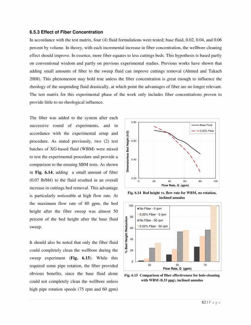
82 | P a g e

6.5.3 Effect of Fiber Concentration

In accordance with the test matrix, four (4) fluid formulations were tested; base fluid, 0.02, 0.04, and 0.06

percent by volume. In theory, with each incremental increase in fiber concentration, the wellbore cleaning

effect should improve. In essence, more fiber equates to less cuttings beds. This hypothesis is based partly

on conventional wisdom and partly on previous experimental studies. Previous works have shown that

adding small amounts of fiber to the sweep fluid can improve cuttings removal (Ahmed and Takach

2008). This phenomenon may hold true unless the fiber concentration is great enough to influence the

rheology of the suspending fluid drastically, at which point the advantages of fiber are no longer relevant.

The test matrix for this experimental phase of the work only includes fiber concentrations proven to

provide little to no rheological influence.

The fiber was added to the system after each

successive round of experiments, and in

accordance with the experimental setup and

procedure. As stated previously, two (2) test

batches of XG-based fluid (WBM) were mixed

to test the experimental procedure and provide a

comparison to the ensuing SBM tests. As shown

in Fig. 6.14, adding a small amount of fiber

(0.07 lb/bbl) to the fluid resulted in an overall

increase in cuttings bed removal. This advantage

is particularly noticeable at high flow rate. At

the maximum flow rate of 80 gpm, the bed

height after the fiber sweep was almost 50

percent of the bed height after the base fluid

sweep.

It should also be noted that only the fiber fluid

could completely clean the wellbore during the

sweep experiment (Fig. 6.15). While this

required some pipe rotation, the fiber provided

obvious benefits, since the base fluid alone

could not completely clean the wellbore unless

high pipe rotation speeds (75 rpm and 60 gpm)

Fig. 6.14 Bed height vs. flow rate for WBM, no rotation,

inclined annulus

Fig. 6.15 Comparison of fiber effectiveness for hole-cleaning

with WBM (8.33 ppg), inclined annulus

0.20

0.40

0.60

0.80

0 20 40 60 80 100

Dim

en

sio

nle

ss

Be

d H

eig

ht

(h/D

)

Flow Rate, Q (gpm)

Base Fluid

0.02% Fiber

0

20

40

60

80

100

30 50 70

% B

ed

He

igh

t R

ed

uc

tio

n

Flow Rate, Q (gpm)

No Fiber - 0 rpm

0.02% Fiber - 0 rpm

No Fiber - 50 rpm

0.02% Fiber - 50 rpm

83 | P a g e

were applied.

Introducing fiber into the weighted synthetic-based fluid (SBM) provided slightly different results. Due to

the weight of the fluid, the inertial force of the moving fluid in the annulus was greater than that of the

unweighted XG-based fluid. This factor alone could have provided enhanced hole-cleaning performance

over the WBM. The inertia of the SBM could have limited the significance of the addition of the fiber. As

shown in Figs. 6.16 to 6.18, the addition of fiber in the horizontal and inclined annulus, without pipe

rotation, provided no real predictable or reliable benefit to cuttings bed eradication. This was in contrast

with the results from the WBM sweep experiments, in which the addition of a small amount of fiber

resulted in a decrease in bed height over the base fluid (Fig. 6.14).

When the annulus was in the horizontal position, the inertial force pushing the cuttings through the

annulus was at the maximum. This left little room for improvement with the addition of fiber. However,

in the inclined position, the cuttings wanted to slide down the annulus, creating more work for the sweep

fluid. Critical evaluation of Fig. 6.18 showed that in the inclined position, the high concentration fiber

sweep provided visual and measurable improved wellbore cleaning over the base fluid. This trend was

slightly apparent at low flow rates, but it became unequivocally obvious at high flow rates. The addition

of fiber may have increased the lifting capacity of the sweep fluid, which enabled the fluid to carry the

cuttings through the annulus and return them to the collection/accumulation tank.

(a)

(b)

Fig. 6.16 Dimensionless bed height vs. flow rate for SBM, no pipe rotation

a) Horizontal annulus, and b) Inclined annulus

0.00

0.20

0.40

0.60

0.80

0 20 40 60 80

Dim

en

sio

nle

ss B

ed

He

igh

t (h

/D)

Flow Rate, Q (gpm)

Base Fluid

0.02% Fiber

0.04% Fiber

0.06% Fiber

0.00

0.20

0.40

0.60

0.80

0 20 40 60 80

Dim

en

sio

nle

ss B

ed

He

igh

t (h

/D)

Flow Rate, Q (gpm)

Base Fluid

0.02% Fiber

0.04% Fiber

0.06% Fiber

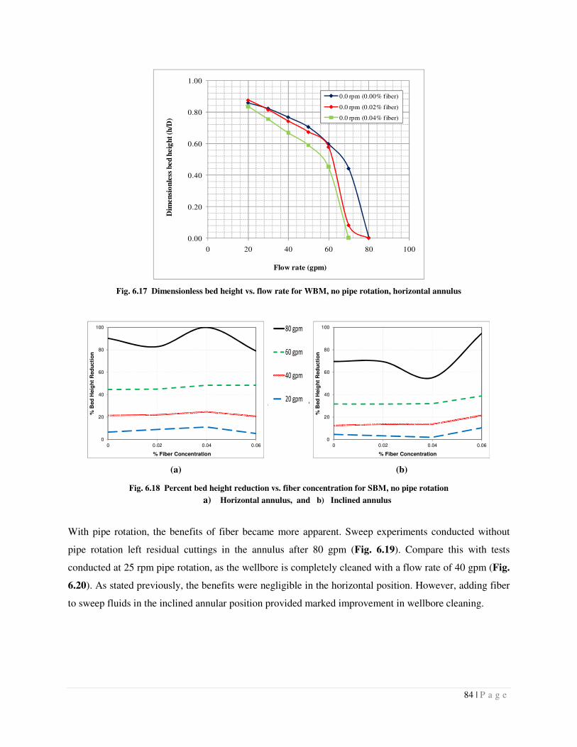
84 | P a g e

Fig. 6.17 Dimensionless bed height vs. flow rate for WBM, no pipe rotation, horizontal annulus

(a)

(b)

Fig. 6.18 Percent bed height reduction vs. fiber concentration for SBM, no pipe rotation


With pipe rotation, the benefits of fiber became more apparent. Sweep experiments conducted without

pipe rotation left residual cuttings in the annulus after 80 gpm (Fig. 6.19). Compare this with tests

conducted at 25 rpm pipe rotation, as the wellbore is completely cleaned with a flow rate of 40 gpm (Fig.

6.20). As stated previously, the benefits were negligible in the horizontal position. However, adding fiber

to sweep fluids in the inclined annular position provided marked improvement in wellbore cleaning.

0.00

0.20

0.40

0.60

0.80

1.00

0 20 40 60 80 100

Dim

en

sio

nle

ss b

ed

heig

ht

(h/D

)

Flow rate (gpm)

0.0 rpm (0.00% fiber)

0.0 rpm (0.02% fiber)

0.0 rpm (0.04% fiber)

0

20

40

60

80

100

0 0.02 0.04 0.06

% B

ed

Heig

ht

Red

ucti

on

% Fiber Concentration

80 gpm

60 gpm

40 gpm

20 gpm

0

20

40

60

80

100

0 0.02 0.04 0.06

% B

ed

Heig

ht

Red

ucti

on


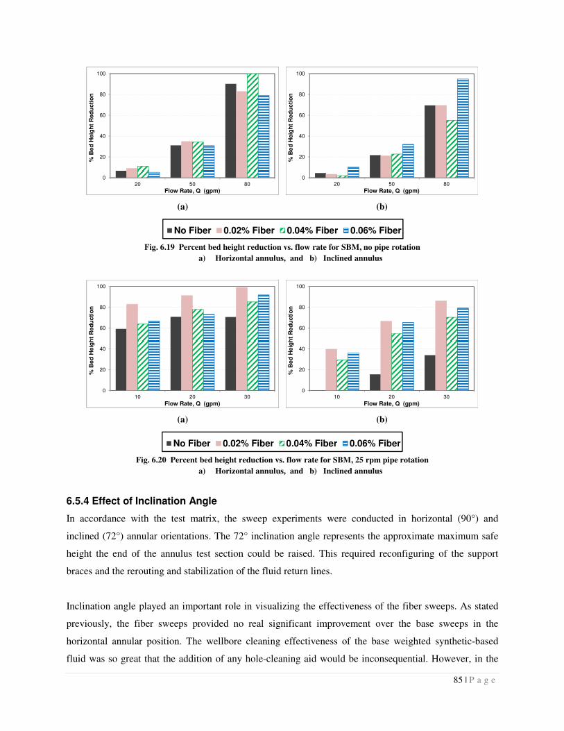
85 | P a g e

(a)

(b)

Fig. 6.19 Percent bed height reduction vs. flow rate for SBM, no pipe rotation


(a)

(b)

Fig. 6.20 Percent bed height reduction vs. flow rate for SBM, 25 rpm pipe rotation


6.5.4 Effect of Inclination Angle

In accordance with the test matrix, the sweep experiments were conducted in horizontal (90°) and

inclined (72°) annular orientations. The 72° inclination angle represents the approximate maximum safe

height the end of the annulus test section could be raised. This required reconfiguring of the support

braces and the rerouting and stabilization of the fluid return lines.

Inclination angle played an important role in visualizing the effectiveness of the fiber sweeps. As stated

previously, the fiber sweeps provided no real significant improvement over the base sweeps in the

horizontal annular position. The wellbore cleaning effectiveness of the base weighted synthetic-based

fluid was so great that the addition of any hole-cleaning aid would be inconsequential. However, in the

0

20

40

60

80

100

20 50 80

% B

ed

He

igh

t R

ed

ucti

on

Flow Rate, Q (gpm)

0

20

40

60

80

100

20 50 80

% B

ed

Heig

ht

Re

du

cti

on

Flow Rate, Q (gpm)

100

No Fiber 0.02% Fiber 0.04% Fiber 0.06% Fiber

0

20

40

60

80

100

10 20 30

% B

ed

Heig

ht

Re

du

cti

on

Flow Rate, Q (gpm)

0

20

40

60

80

100

10 20 30

% B

ed

Heig

ht

Re

du

cti

on

Flow Rate, Q (gpm)

100

No Fiber 0.02% Fiber 0.04% Fiber 0.06% Fiber

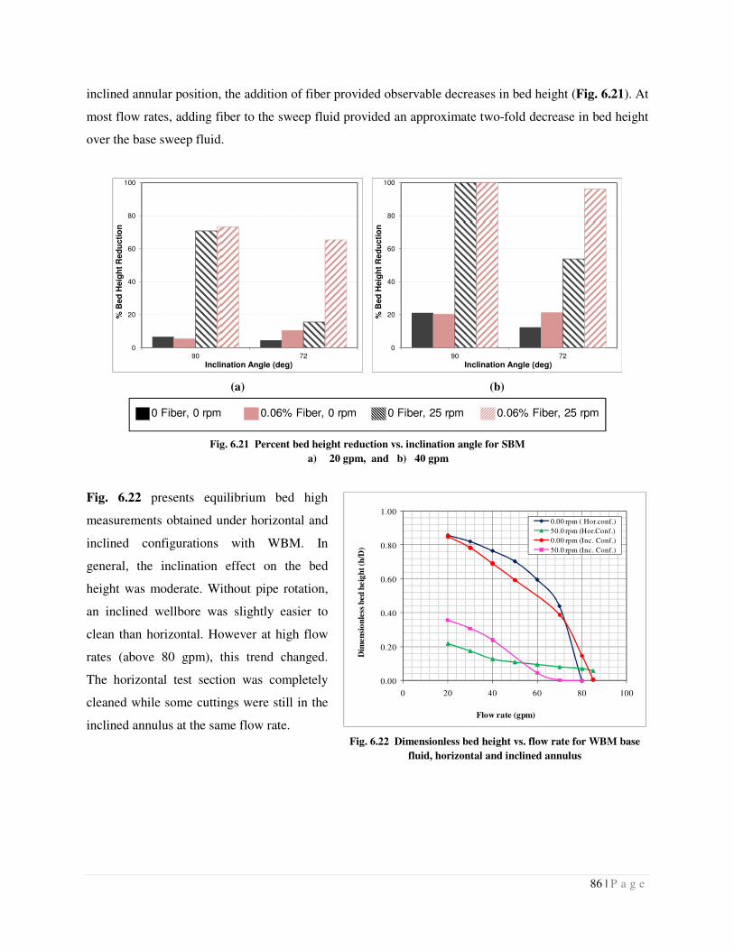
86 | P a g e

inclined annular position, the addition of fiber provided observable decreases in bed height (Fig. 6.21). At

most flow rates, adding fiber to the sweep fluid provided an approximate two-fold decrease in bed height

over the base sweep fluid.

(a)

(b)

Fig. 6.21 Percent bed height reduction vs. inclination angle for SBM

a) 20 gpm, and b) 40 gpm

Fig. 6.22 presents equilibrium bed high

measurements obtained under horizontal and

inclined configurations with WBM. In

general, the inclination effect on the bed

height was moderate. Without pipe rotation,

an inclined wellbore was slightly easier to

clean than horizontal. However at high flow

rates (above 80 gpm), this trend changed.

The horizontal test section was completely

cleaned while some cuttings were still in the

inclined annulus at the same flow rate.

0

20

40

60

80

100

90 72

% B

ed

He

igh

t R

ed

ucti

on

Inclination Angle (deg)

0

20

40

60

80

100

90 72

% B

ed

He

igh

t R

ed

ucti

on

Inclination Angle (deg)

0.06% Fiber, 25 rpm0 Fiber, 25 rpm0.06% Fiber, 0 rpm0 Fiber, 0 rpm

Fig. 6.22 Dimensionless bed height vs. flow rate for WBM base

fluid, horizontal and inclined annulus

0.00

0.20

0.40

0.60

0.80

1.00

0 20 40 60 80 100

Dim

en

sio

nle

ss b

ed

heig

ht

(h/D

)

Flow rate (gpm)

0.00 rpm ( Hor.conf.)

50.0 rpm (Hor.Conf.)

0.00 rpm (Inc. Conf.)

50.0 rpm (Inc. Conf.)

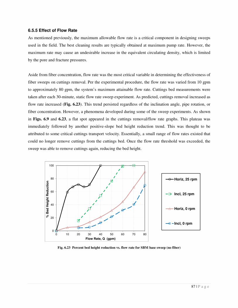
87 | P a g e

6.5.5 Effect of Flow Rate

As mentioned previously, the maximum allowable flow rate is a critical component in designing sweeps

used in the field. The best cleaning results are typically obtained at maximum pump rate. However, the

maximum rate may cause an undesirable increase in the equivalent circulating density, which is limited

by the pore and fracture pressures.

Aside from fiber concentration, flow rate was the most critical variable in determining the effectiveness of

fiber sweeps on cuttings removal. Per the experimental procedure, the flow rate was varied from 10 gpm

to approximately 80 gpm, the system’s maximum attainable flow rate. Cuttings bed measurements were

taken after each 30-minute, static flow rate sweep experiment. As predicted, cuttings removal increased as

flow rate increased (Fig. 6.23). This trend persisted regardless of the inclination angle, pipe rotation, or

fiber concentration. However, a phenomena developed during some of the sweep experiments. As shown

in Figs. 6.9 and 6.23, a flat spot appeared in the cuttings removal/flow rate graphs. This plateau was

immediately followed by another positive-slope bed height reduction trend. This was thought to be

attributed to some critical cuttings transport velocity. Essentially, a small range of flow rates existed that

could no longer remove cuttings from the cuttings bed. Once the flow rate threshold was exceeded, the

sweep was able to remove cuttings again, reducing the bed height.

Fig. 6.23 Percent bed height reduction vs. flow rate for SBM base sweep (no fiber)

0

20

40

60

80

100

0 10 20 30 40 50 60 70 80

% B

ed

Heig

ht

Re

du

cti

on

Flow Rate, Q (gpm)

Horiz, 25 rpm

Incl, 25 rpm

Horiz, 0 rpm

Incl, 0 rpm

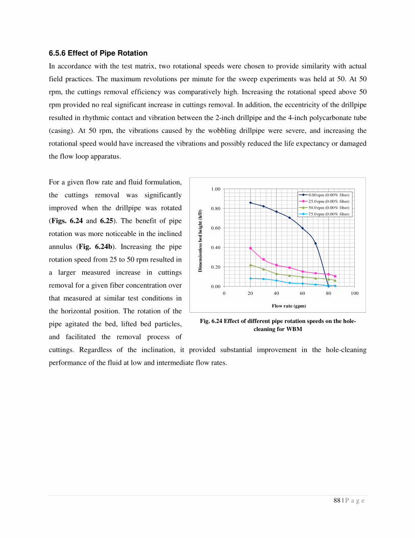
88 | P a g e

6.5.6 Effect of Pipe Rotation

In accordance with the test matrix, two rotational speeds were chosen to provide similarity with actual

field practices. The maximum revolutions per minute for the sweep experiments was held at 50. At 50

rpm, the cuttings removal efficiency was comparatively high. Increasing the rotational speed above 50

rpm provided no real significant increase in cuttings removal. In addition, the eccentricity of the drillpipe

resulted in rhythmic contact and vibration between the 2-inch drillpipe and the 4-inch polycarbonate tube

(casing). At 50 rpm, the vibrations caused by the wobbling drillpipe were severe, and increasing the

rotational speed would have increased the vibrations and possibly reduced the life expectancy or damaged

the flow loop apparatus.

For a given flow rate and fluid formulation,

the cuttings removal was significantly

improved when the drillpipe was rotated

(Figs. 6.24 and 6.25). The benefit of pipe

rotation was more noticeable in the inclined

annulus (Fig. 6.24b). Increasing the pipe

rotation speed from 25 to 50 rpm resulted in

a larger measured increase in cuttings

removal for a given fiber concentration over

that measured at similar test conditions in

the horizontal position. The rotation of the

pipe agitated the bed, lifted bed particles,

and facilitated the removal process of

cuttings. Regardless of the inclination, it provided substantial improvement in the hole-cleaning

performance of the fluid at low and intermediate flow rates.

Fig. 6.24 Effect of different pipe rotation speeds on the hole-

cleaning for WBM

0.00

0.20

0.40

0.60

0.80

1.00

0 20 40 60 80 100

Dim

ensi

on

less

bed

heig

ht

(h/D

)

Flow rate (gpm)

0.00 rpm (0.00% fiber)

25.0 rpm (0.00% fiber)

50.0 rpm (0.00% fiber)

75.0 rpm (0.00% fiber)

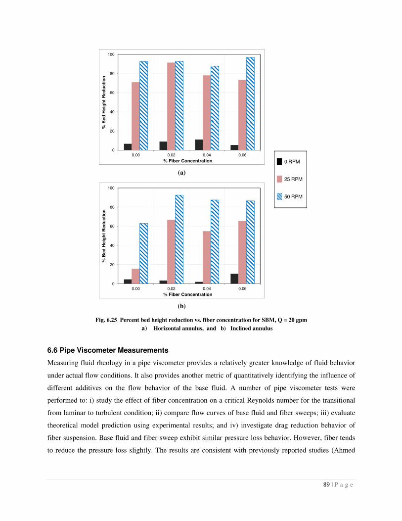
89 | P a g e

(a)

(b)

Fig. 6.25 Percent bed height reduction vs. fiber concentration for SBM, Q = 20 gpm


6.6 Pipe Viscometer Measurements

Measuring fluid rheology in a pipe viscometer provides a relatively greater knowledge of fluid behavior

under actual flow conditions. It also provides another metric of quantitatively identifying the influence of

different additives on the flow behavior of the base fluid. A number of pipe viscometer tests were

performed to: i) study the effect of fiber concentration on a critical Reynolds number for the transitional

from laminar to turbulent condition; ii) compare flow curves of base fluid and fiber sweeps; iii) evaluate

theoretical model prediction using experimental results; and iv) investigate drag reduction behavior of

fiber suspension. Base fluid and fiber sweep exhibit similar pressure loss behavior. However, fiber tends

to reduce the pressure loss slightly. The results are consistent with previously reported studies (Ahmed

0

20

40

60

80

100

0.00 0.02 0.04 0.06

% B

ed

Heig

ht

Red

ucti

on

% Fiber Concentration 0 RPM

25 RPM

50 RPM

0

20

40

60

80

100

0.00 0.02 0.04 0.06

% B

ed

Heig

ht

Red

ucti

on


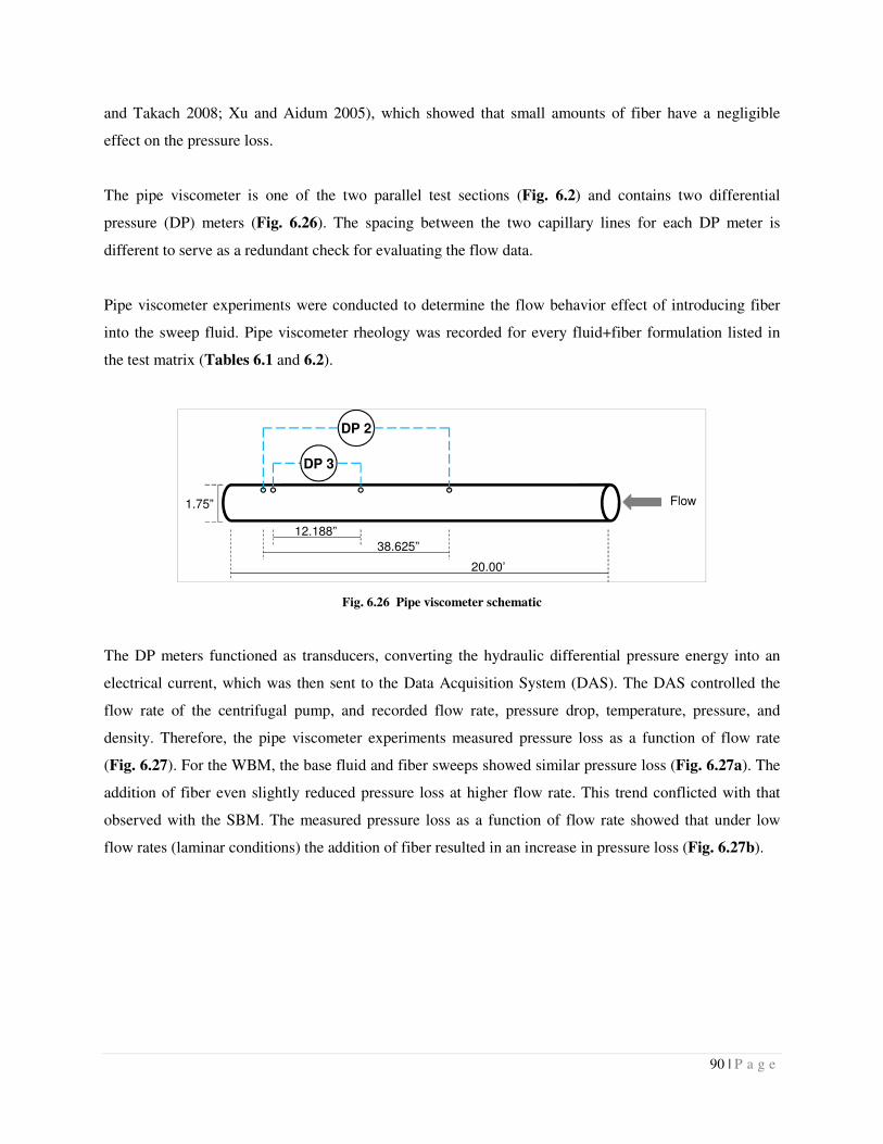
90 | P a g e

and Takach 2008; Xu and Aidum 2005), which showed that small amounts of fiber have a negligible

effect on the pressure loss.

The pipe viscometer is one of the two parallel test sections (Fig. 6.2) and contains two differential

pressure (DP) meters (Fig. 6.26). The spacing between the two capillary lines for each DP meter is

different to serve as a redundant check for evaluating the flow data.

Pipe viscometer experiments were conducted to determine the flow behavior effect of introducing fiber

into the sweep fluid. Pipe viscometer rheology was recorded for every fluid+fiber formulation listed in

the test matrix (Tables 6.1 and 6.2).

Fig. 6.26 Pipe viscometer schematic

The DP meters functioned as transducers, converting the hydraulic differential pressure energy into an

electrical current, which was then sent to the Data Acquisition System (DAS). The DAS controlled the

flow rate of the centrifugal pump, and recorded flow rate, pressure drop, temperature, pressure, and

density. Therefore, the pipe viscometer experiments measured pressure loss as a function of flow rate

(Fig. 6.27). For the WBM, the base fluid and fiber sweeps showed similar pressure loss (Fig. 6.27a). The

addition of fiber even slightly reduced pressure loss at higher flow rate. This trend conflicted with that

observed with the SBM. The measured pressure loss as a function of flow rate showed that under low

flow rates (laminar conditions) the addition of fiber resulted in an increase in pressure loss (Fig. 6.27b).

DP 2

DP 3

12.188”

38.625”

Flow

20.00’

1.75”

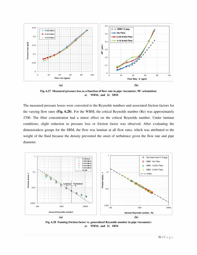
91 | P a g e

(a)

(b)

Fig. 6.27 Measured pressure loss as a function of flow rate in pipe viscometer, 90° orientation:

a) WBM; and b) SBM

The measured pressure losses were converted to the Reynolds numbers and associated friction factors for

the varying flow rates (Fig. 6.28). For the WBM, the critical Reynolds number (Re) was approximately

2700. The fiber concentration had a minor effect on the critical Reynolds number. Under laminar

conditions, slight reduction in pressure loss or friction factor was observed. After evaluating the

dimensionless groups for the SBM, the flow was laminar at all flow rates, which was attributed to the

weight of the fluid because the density prevented the onset of turbulence given the flow rate and pipe

diameter.

(a)

(b)

Fig. 6.28 Fanning friction factor vs. generalized Reynolds number in pipe viscometer:

a) WBM; and b) SBM

0

0.1

0.2

0.3

0.4

0.5

0.6

0 20 40 60 80 100

∆P

(

ps

i )

Flow Rate, Q (gpm)

SBM-7.5 ppg

No Fiber

0.09 lb/bbl Fiber

0.18 lb/bbl Fiber

0.001

0.01

0.1

1

100 1000 10000

Fr

icti

on

fa

cto

r,

f

General Reynolds number

Predicted

0.00%fiber

0.02%fiber

0.04%fiber

0.06%fiber

16/Re

TurbulentLaminar

0.001

0.01

0.1

1

100 1000 10000

Fri

cti

on

fa

cto

r,

f

General Reynolds number, Re

Syn-base fluid (7.5 ppg)

SBM - No Fiber

SBM - 0.02% Fiber

SBM - 0.04% Fiber

16/Re

0

0.05

0.1

0.15

0.2

0.25

0 20 40 60 80 100

Pre

ssu

re l

oss

(p

si)

Flow rate (gpm)

0.00%fiber

0.02%fiber

0.04%fiber

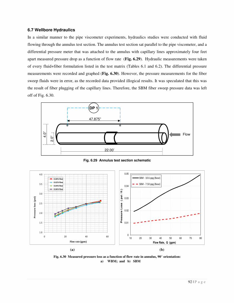
92 | P a g e

6.7 Wellbore Hydraulics

In a similar manner to the pipe viscometer experiments, hydraulics studies were conducted with fluid

flowing through the annulus test section. The annulus test section sat parallel to the pipe viscometer, and a

differential pressure meter that was attached to the annulus with capillary lines approximately four feet

apart measured pressure drop as a function of flow rate (Fig. 6.29). Hydraulic measurements were taken

of every fluid+fiber formulation listed in the test matrix (Tables 6.1 and 6.2). The differential pressure

measurements were recorded and graphed (Fig. 6.30). However, the pressure measurements for the fiber

sweep fluids were in error, as the recorded data provided illogical results. It was speculated that this was

the result of fiber plugging of the capillary lines. Therefore, the SBM fiber sweep pressure data was left

off of Fig. 6.30.

(a)

(b)

Fig. 6.30 Measured pressure loss as a function of flow rate in annulus, 90° orientation:

a) WBM; and b) SBM

1.0

1.5

2.0

2.5

3.0

3.5

4.0

0 20 40 60

Pr

es

su

re

lo

ss

(p

si)

Flow rate (gpm)

0.00% fiber

0.02% fiber

0.04% fiber

0.06% fiber

0

0.01

0.02

0.03

0.04

0.05

10 20 30 40 50 60 70 80

Pres

su

re L

oss

(

ps

i / ft

)

Flow Rate, Q (gpm)

SBM - 10.6 ppg (Base)

SBM - 7.50 ppg (Base)

Fig. 6.29 Annulus test section schematic

DP 1

47.875”

Flow

22.00’

4.0

”

2.0

”

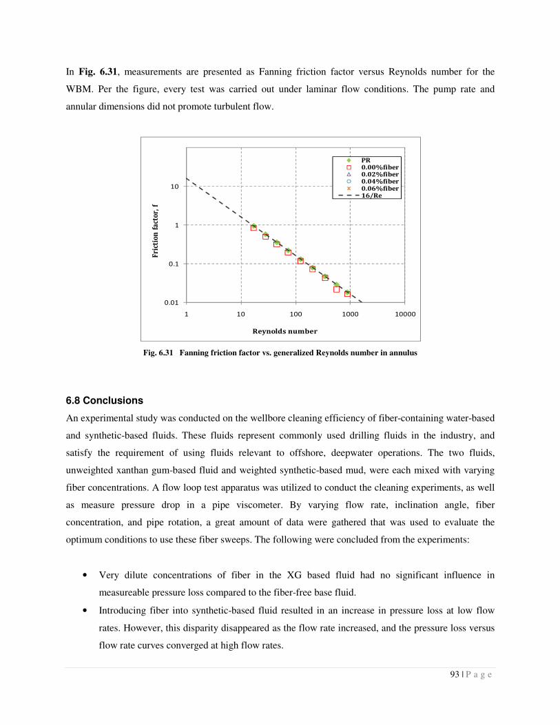
93 | P a g e

In Fig. 6.31, measurements are presented as Fanning friction factor versus Reynolds number for the

WBM. Per the figure, every test was carried out under laminar flow conditions. The pump rate and

annular dimensions did not promote turbulent flow.

Fig. 6.31 Fanning friction factor vs. generalized Reynolds number in annulus

6.8 Conclusions

An experimental study was conducted on the wellbore cleaning efficiency of fiber-containing water-based

and synthetic-based fluids. These fluids represent commonly used drilling fluids in the industry, and

satisfy the requirement of using fluids relevant to offshore, deepwater operations. The two fluids,

unweighted xanthan gum-based fluid and weighted synthetic-based mud, were each mixed with varying

fiber concentrations. A flow loop test apparatus was utilized to conduct the cleaning experiments, as well

as measure pressure drop in a pipe viscometer. By varying flow rate, inclination angle, fiber

concentration, and pipe rotation, a great amount of data were gathered that was used to evaluate the

optimum conditions to use these fiber sweeps. The following were concluded from the experiments:

• Very dilute concentrations of fiber in the XG based fluid had no significant influence in

measureable pressure loss compared to the fiber-free base fluid.

• Introducing fiber into synthetic-based fluid resulted in an increase in pressure loss at low flow

rates. However, this disparity disappeared as the flow rate increased, and the pressure loss versus

flow rate curves converged at high flow rates.

0.01

0.1

1

10

1 10 100 1000 10000

Fri

ctio

n f

act

or,

f

Reynolds number

PR0.00%fiber0.02%fiber0.04%fiber0.06%fiber16/Re

94 | P a g e

• For a non-rotating pipe case, noticeable increase in cuttings removal was not observed with

increasing fiber concentration. The inertia of the weighted fluid is great enough to mask any

slight improvement that might be gained by adding fiber to the system.

• With pipe rotation, cuttings removal increased with the introduction of fiber to the system. Only a

slight amount of fiber was necessary to observe the improved wellbore cleaning performance of

the fiber sweep over the base fluid sweep.

• Maximum wellbore cleaning performance with a very dilute concentration of fiber was achieved

at maximum flow rate and pipe rotation.

6.9 Guidelines

The applicability of this study to the industry is apparent in the experimental results. As this study was

oriented towards offshore, deepwater drilling operations, the results regarding oil-based muds and

synthetic-based muds are of the utmost importance. The rheological studies implicate that the addition of

fiber up to 0.08 percent will have no significant impact of rheology, and subsequently the hydraulics and

ECD will remain unaffected. The sweep experiments and pipe viscometer rheology also reinforce the

usefulness of fiber in sweep fluids. Under similar conditions, fiber sweeps improved wellbore cleaning

over base fluid sweeps. Taking this into consideration, the recommendations here-to-fore in the use of

fiber-containing sweeps are as follows:

• Utilize base sweep fluids that have gelling property (i.e., measurable yield stress). The presence

of yield stress is necessary to achieve stable and homogeneous suspension of fiber particles

within the sweep fluid.

• Use fiber concentration of approximately 0.04 percent. As shown in Section 5.3.4, the best hole-

cleaning performance is generally achieved with an optimum fiber concentration that makes the

fiber drag comparable with the viscous drag force. Increasing fiber concentration beyond this

optimum value results in minimal cleaning improvement. In addition, using optimum fiber

concentration will ensure a minimal ECD influence.

• Rotate the drillstring while applying fiber sweep material to optimize wellbore cleaning. Without

drillstring rotation, the performance improvement obtained from the application of fiber sweep is

minimal.

95 | P a g e

Nomenclature

bbl = Barrel

cp = Centipoise

DAS = Data acquisition system

DP = Differential pressure


gpm = Gallons per minute



ppg = Pounds per gallon

Q = Flow rate

Re = Reynolds number

rpm = Rotations per minute

SBM = Synthetic-based mud

Ty = yield stress

WBM = Water-based mud

XG = Xanthan Gum

Greek Letters

θ = Inclination angle �� = Shear rate


96 | P a g e

References

Ahmed, R.M. & Takach, N.E. 2008. Fiber Sweeps for Hole Cleaning. Paper SPE 113746 presented at the

SPE/ICoTA Coiled Tubing and Well Intervention Conference and Exhibition, The Woodlands,

Texas, 1-2 April.

Bulgachev, R.V. & Pouget, P. 2006. New Experience in Monofilament Fiber Tandem Sweeps Hole

Cleaning Performance on Kharyaga Oilfield, Timan-Pechora Region of Russia. Paper SPE

101961 presented at the SPE Russian Oil and Gas Technical Conference and Exhibition,

Moscow, Russia, 3-6 October.

Cameron, C., Helmy, H., & Haikal, M. 2003. Fibrous LCM Sweeps Enhance Hole Cleaning and ROP on

Extended Reach Well in Abu Dhabi. Paper SPE 81419 presented at the SPE 13th Middle East Oil

Show and Conference, Bahrain, 5-8 April.

George, M.L., Ahmed, R.M. & Growcock, F.B. 2011. Rheological Properties of Fiber-Containing

Drilling Sweeps at Ambient and High Temperature Conditions. Paper AADE-11-NTCE-35

presented at the AADE National Technical Conference & Exhibition, Houston, Texas, USA, 12-

14 April.

Guo, R., Azaiez, J., & Bellehumeur, C. 2005. Rheology of Fiber Filled Polymer Melts: Role of Fiber-

Fiber Interactions and Polymer-Fiber Coupling. Polymer Eng. and Sci. 45 (3): 385-399.

Hemphill, T. & Rojas, J.C. 2002. Drilling Fluid Sweeps: Their Evaluation, Timing, and Applications.

Paper SPE 77448 presented at the SPE Annual Technical Conference and Exhibition, San

Antonio, Texas, 29 September-2 October.

Marti, I., Hofler, O., Fischer, P. & Windhab, E.J. 2005. Rheology of Concentrated Suspensions

Containing Mixtures of Spheres and Fibres. Rheologica Acta 44 (5): 502–512

Rajabian, M., Dubois, C., & Grmela, M. 2005. Suspensions of Semiflexible Fibers in Polymeric Fluids:

Rheology and Thermodynamics. Rheologica Acta 44 (5): 521–535.

Valluri, S.G., Miska, S.Z., Ahmed, R.M. & Takach, N.E. 2006. Experimental Study of Effective Hole

Cleaning Using “Sweeps” in Horizontal Wellbores. Paper SPE 101220 presented at the SPE

Annual Technical Conference and Exhibition, San Antonio, Texas, 24-27 September.

97 | P a g e

7. Mechanistic Modeling of Hole Cleaning with Fiber Sweeps

The mechanistic model presented in this study is an extension of existing cuttings transport models

(Ahmed et al. 2002; Duan 2005; Larsen et al. 1997; Clark et al. 1994). It was developed to predict critical

transport velocity (CTV) in fiber-containing fluid. The CTV for fiber-containing fluid is different from

that of the fluid without fiber (base fluid). Adding fiber to the base fluid creates additional force, fiber

drag force, acting on bed particles in the same direction as the viscous drag force. The fiber drag can

initiate particle movement even at low fluid velocities in which the viscous drag is minimal. As shown in

Eqn. (5.7), the fiber drag is a function of the fiber drag coefficient, and a reliable correlation is needed to

estimate the coefficient. A mathematical model for the CTV has been developed considering linear and

angular momentum balances of a bed particle.

7.1 Introduction

Mathematical hole-cleaning models are often preferred because of their wide range of applicability. Clark

and Bickham (1994) presented a mechanistic model for predicting the minimum fluid velocity for

transporting cuttings without formation of a cuttings bed. This model considers major forces acting on a

single stationary cuttings particle deposited on the surface of the bed. To verify the model, they performed

flow loop tests using different test fluids (water, solution of HEC, and xanthan gum). The tests were run

at angles ranging from near vertical (20° minimum) to horizontal (90°). The model prediction showed a

good agreement with the experimental results. Recently, an improved mechanistic model (Ahmed et al.

2002) was developed to predict the critical transport velocity (CTV). The model was verified using

experimental data obtained using water and polypnoinic cellulose suspension as test fluids. The average

cuttings size was varied from 0.125 mm to 3.5 mm. The model predictions showed satisfactory agreement

with experimental measurements.

Although mechanistic models provide general CTV predictions for different drilling applications, their

accuracy is lower than that of the empirical models. To improve the accuracy of the mechanistic models,

studies were conducted to develop models that combine both mechanistic models and empirical

correlations. Rasi (1994) presented a semi-empirical model that combines fluid mechanics-based

analytical model with correlations developed using experimental and field data. Later, an improved semi-

empirical model (Larson et al. 1997) was developed to predict the required critical transport velocity in

high angle wells. The model was developed after performing an extensive experimental study using a

medium-scale flow loop. The model predicted critical transport velocity and annular cuttings

concentration under different drilling conditions for highly deviated and horizontal wells. The study

concluded that cuttings start to accumulate in the wellbore if the annular velocity becomes insufficient,

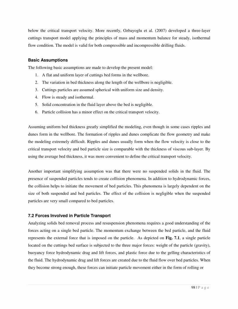
98 | P a g e

below the critical transport velocity. More recently, Ozbayoglu et al. (2007) developed a three-layer

cuttings transport model applying the principles of mass and momentum balance for steady, isothermal

flow condition. The model is valid for both compressible and incompressible drilling fluids.

Basic Assumptions

The following basic assumptions are made to develop the present model:

1. A flat and uniform layer of cuttings bed forms in the wellbore.

2. The variation in bed thickness along the length of the wellbore is negligible.

3. Cuttings particles are assumed spherical with uniform size and density.

4. Flow is steady and isothermal.

5. Solid concentration in the fluid layer above the bed is negligible.

6. Particle collision has a minor effect on the critical transport velocity.

Assuming uniform bed thickness greatly simplified the modeling, even though in some cases ripples and

dunes form in the wellbore. The formation of ripples and dunes complicate the flow geometry and make

the modeling extremely difficult. Ripples and dunes usually form when the flow velocity is close to the

critical transport velocity and bed particle size is comparable with the thickness of viscous sub-layer. By

using the average bed thickness, it was more convenient to define the critical transport velocity.

Another important simplifying assumption was that there were no suspended solids in the fluid. The

presence of suspended particles tends to create collision phenomena. In addition to hydrodynamic forces,

the collision helps to initiate the movement of bed particles. This phenomena is largely dependent on the

size of both suspended and bed particles. The effect of the collision is negligible when the suspended

particles are very small compared to bed particles.

7.2 Forces Involved in Particle Transport

Analyzing solids bed removal process and resuspension phenomena requires a good understanding of the

forces acting on a single bed particle. The momentum exchange between the bed particle, and the fluid

represents the external force that is imposed on the particle. As depicted on Fig. 7.1, a single particle

located on the cuttings bed surface is subjected to the three major forces: weight of the particle (gravity),

buoyancy force hydrodynamic drag and lift forces, and plastic force due to the gelling characteristics of

the fluid. The hydrodynamic drag and lift forces are created due to the fluid flow over bed particles. When

they become strong enough, these forces can initiate particle movement either in the form of rolling or

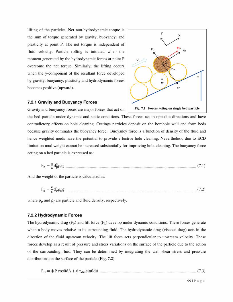
99 | P a g e

lifting of the particles. Net non-hydrodynamic torque is

the sum of torque generated by gravity, buoyancy, and

plasticity at point P. The net torque is independent of

fluid velocity. Particle rolling is initiated when the

moment generated by the hydrodynamic forces at point P

overcome the net torque. Similarly, the lifting occurs

when the y-component of the resultant force developed

by gravity, buoyancy, plasticity and hydrodynamic forces

becomes positive (upward).

7.2.1 Gravity and Buoyancy Forces

Gravity and buoyancy forces are major forces that act on

the bed particle under dynamic and static conditions. These forces act in opposite directions and have

contradictory effects on hole cleaning. Cuttings particles deposit on the borehole wall and form beds

because gravity dominates the buoyancy force. Buoyancy force is a function of density of the fluid and

hence weighted muds have the potential to provide effective hole cleaning. Nevertheless, due to ECD

limitation mud weight cannot be increased substantially for improving hole-cleaning. The buoyancy force

acting on a bed particle is expressed as:

F� cU d�5ρ�g (7.1)

And the weight of the particle is calculated as:

F� cU d�5ρ�g (7.2)

where ρ� and ρ� are particle and fluid density, respectively.

7.2.2 Hydrodynamic Forces

The hydrodynamic drag (FD) and lift force (FL) develop under dynamic conditions. These forces generate

when a body moves relative to its surrounding fluid. The hydrodynamic drag (viscous drag) acts in the

direction of the fluid upstream velocity. The lift force acts perpendicular to upstream velocity. These

forces develop as a result of pressure and stress variations on the surface of the particle due to the action

of the surrounding fluid. They can be determined by integrating the wall shear stress and pressure

distributions on the surface of the particle (Fig. 7.2):

F� ∮PcosθdA @ ∮τk(sinθdA (7.3)

Fig. 7.1 Forces acting on single bed particle

Ф

α

FL

FP

W

FD

P

U

FDf

Xy

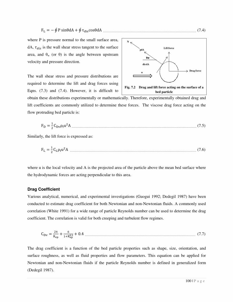
100 | P a g e

Fm �∮PsinθdA @ ∮τk(cosθdA (7.4) where P is pressure normal to the small surface area,

dA, nopF is the wall shear stress tangent to the surface

area, and θw (or θ) is the angle between upstream

velocity and pressure direction.

The wall shear stress and pressure distributions are

required to determine the lift and drag forces using

Eqns. (7.3) and (7.4). However, it is difficult to

obtain these distributions experimentally or mathematically. Therefore, experimentally obtained drag and

lift coefficients are commonly utilized to determine these forces. The viscose drag force acting on the

flow protruding bed particle is:

F� ��C��ρ�u�A (7.5)

Similarly, the lift force is expressed as:

Fm ��Cmρ�u�A (7.6)

where u is the local velocity and A is the projected area of the particle above the mean bed surface where

the hydrodynamic forces are acting perpendicular to this area.

Drag Coefficient

Various analytical, numerical, and experimental investigations (Guogui 1992; Dedegil 1987) have been

conducted to estimate drag coefficient for both Newtonian and non-Newtonian fluids. A commonly used

correlation (White 1991) for a wide range of particle Reynolds number can be used to determine the drag

coefficient. The correlation is valid for both creeping and turbulent flow regimes.

C�� 4rs� @ U�.rs�t.u @ 0.4 (7.7)

The drag coefficient is a function of the bed particle properties such as shape, size, orientation, and

surface roughness, as well as fluid properties and flow parameters. This equation can be applied for

Newtonian and non-Newtonian fluids if the particle Reynolds number is defined in generalized form

(Dedegil 1987).

Fig. 7.2 Drag and lift force acting on the surface of a

bed particle

Drag force

Lift force

θw

pdA

�dis dA

N

u

101 | P a g e

Rv� w!��x (7.8)

The shear stress, τ, is evaluated at the representative shear rate of (u/dp). Eqn. (7.7) was developed and

used to predict drag coefficient of a single particle without considering the effect of neighboring particles.

In order to predict reasonable values of drag force, the equation should be modified to account for the

variation of drag coefficient due to the presence of other particles on the surface of the solids bed (Ahmed

et al. 2002). An extensive experimental study (Liang et al. 1995) performed to determine the effect

surrounding particles on drag coefficient presented a correction factor, Dr, which varies from 1.05 to 0.35.

The correction factor is 1.05 without the presence of particles and 0.35 with the presence of several

neighboring particles. Due to the presence of many particles on the surface of the bed, more realistic

value for the correction is 0.35. However, during model testing and calibration, the best drag correction

factor was found to be 0.4.

Lift Coefficient

Lift force exists due to the asymmetry in the flow field around the particle. The asymmetry flow condition

is established because of the no-slip boundary condition at the cuttings bed surface. This phenomenon is

responsible for the lift mechanism. A small spherical particle moving through very viscous liquid in slow

shear flow experiences a lift force resulting from the velocity gradient (Saffman 1964). Two assumptions

are made in the development of Saffman’s lift force equation: i) the particle is not influenced by solid

boundaries, and ii) constant fluid velocity gradient. The equation is expressed as:

Fm 1.615 4�!:y! 6w?7`.S (7.9)

where v is the kinematic viscosity and y is the vertical distance from the mean bed level. The validation of

his formula is limited to instances in which certain values of gradient Reynolds number, Rvz d�Bdu/dyD| , Rep and ReG is less than unity. By combining Eqns. (7.6) and (7.9), lift coefficient can be

expressed as:

Cm 4.11 - �wrs� w?3`.S (7.10)

7.2.3 Fiber Drag Force

When fiber is introduced to pure liquid, an additional drag force will develop if the particle slips in the

fluid or the fluid flows past the particle. Fiber drag force, F��, acts in the same direction as the viscous

drag force (Fig. 7.1). In order to estimate this force, a model has been developed. Even though limited

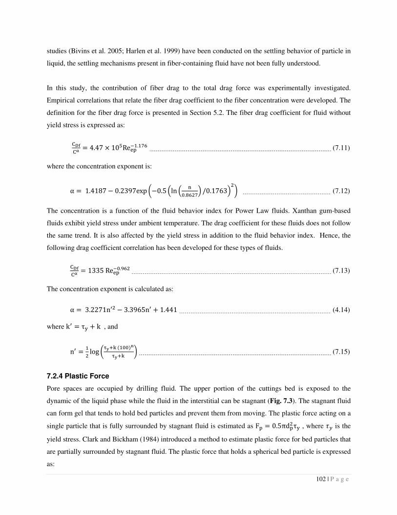
102 | P a g e

studies (Bivins et al. 2005; Harlen et al. 1999) have been conducted on the settling behavior of particle in

liquid, the settling mechanisms present in fiber-containing fluid have not been fully understood.

In this study, the contribution of fiber drag to the total drag force was experimentally investigated.

Empirical correlations that relate the fiber drag coefficient to the fiber concentration were developed. The

definition for the fiber drag force is presented in Section 5.2. The fiber drag coefficient for fluid without

yield stress is expressed as:

��M 4.47 Q 10SRev��.�TU (7.11)

where the concentration exponent is:

α 1.4187 � 0.2397exp /�0.5 6ln 6 �`.aU�T7 /0.17637�2 (7.12)

The concentration is a function of the fluid behavior index for Power Law fluids. Xanthan gum-based

fluids exhibit yield stress under ambient temperature. The drag coefficient for these fluids does not follow

the same trend. It is also affected by the yield stress in addition to the fluid behavior index. Hence, the

following drag coefficient correlation has been developed for these types of fluids.

��M 1335Rev��`.~U� (7.13)

The concentration exponent is calculated as:

α 3.2271n�� 3.3965n� @ 1.441 (4.14) where k� τ? @ k , and

n� �� log /x�.�B�``D�x�.� 2 (7.15)

7.2.4 Plastic Force

Pore spaces are occupied by drilling fluid. The upper portion of the cuttings bed is exposed to the

dynamic of the liquid phase while the fluid in the interstitial can be stagnant (Fig. 7.3). The stagnant fluid

can form gel that tends to hold bed particles and prevent them from moving. The plastic force acting on a

single particle that is fully surrounded by stagnant fluid is estimated as F� 0.5πd��τ? , where n� is the

yield stress. Clark and Bickham (1984) introduced a method to estimate plastic force for bed particles that

are partially surrounded by stagnant fluid. The plastic force that holds a spherical bed particle is expressed

as:

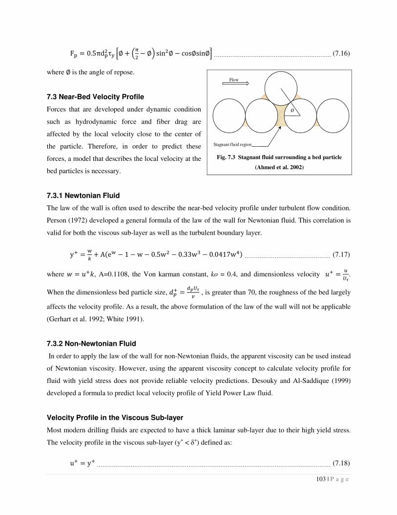
103 | P a g e

F� 0.5πd��τ? �∅ @ 6c� � ∅7 sin�∅ � cos∅sin∅� (7.16)

where ∅is the angle of repose.

7.3 Near-Bed Velocity Profile

Forces that are developed under dynamic condition

such as hydrodynamic force and fiber drag are

affected by the local velocity close to the center of

the particle. Therefore, in order to predict these

forces, a model that describes the local velocity at the

bed particles is necessary.

7.3.1 Newtonian Fluid

The law of the wall is often used to describe the near-bed velocity profile under turbulent flow condition.

Person (1972) developed a general formula of the law of the wall for Newtonian fluid. This correlation is

valid for both the viscous sub-layer as well as the turbulent boundary layer.

y. �� @ ABe� � 1 � w� 0.5w� � 0.33w5 � 0.0417w4D (7.17)

where � �.�, A=0.1108, the Von karman constant, ko = 0.4, and dimensionless velocity �. ��. When the dimensionless bed particle size, H�. o��y , is greater than 70, the roughness of the bed largely

affects the velocity profile. As a result, the above formulation of the law of the wall will not be applicable

(Gerhart et al. 1992; White 1991).

7.3.2 Non-Newtonian Fluid

In order to apply the law of the wall for non-Newtonian fluids, the apparent viscosity can be used instead

of Newtonian viscosity. However, using the apparent viscosity concept to calculate velocity profile for

fluid with yield stress does not provide reliable velocity predictions. Desouky and Al-Saddique (1999)

developed a formula to predict local velocity profile of Yield Power Law fluid.

Velocity Profile in the Viscous Sub-layer

Most modern drilling fluids are expected to have a thick laminar sub-layer due to their high yield stress.

The velocity profile in the viscous sub-layer (y+ < δ+) defined as:

u. y. (7.18)

Fig. 7.3 Stagnant fluid surrounding a bed particle

(Ahmed et al. 2002)

Ø

Stagnant fluid region

Flow

104 | P a g e

where y. is the dimensionless distance from the mean bed surface and is expressed as

y. y�Ux�� 6��7, y is the distance from the mean bed surface, Ux 6x�s�� 7`.S , and n��o is average of

bed shear stress, n��o ��o ��!� . Dimensionless thickness of the laminar sub-layer, δ. is calculated as:

δ. δ�Ux�� 6��7 (7.19)

where

δ S��rs� 6 �K� ¡7`.S (7.20)

Substituting u+ and y+ into Eqn. (7.18) and rearranging it:

u y 6x�s�� B1 � xD7�/� (7.21)

Hence, the local velocity gradient can be determined from the above equation.

w? 6x�s�� B1 � xD7�/� (7.22)

X x�x�s� (7.23)

where n is the fluid behavior index, and K is the consistency index.

Velocity Profile outside the Viscous Sub-layer

Outside the viscous sub-layer, the velocity profile for Yield Power Law fluid is determined using the

following formula.

u £¤� ¥¦1 � �?�§@ ln¨1 � ¦1 � �?�§©ª @ U#=« (7.24)

where U#=« is the maximum fluid velocity that can be expressed as:

U#=« �6x�s�� B1 � xD7��/� δ � £¤�t �1 @ ln 6 ¬�§7� (7.25)

Similarly, the velocity gradient can be obtained from the above equation.

105 | P a g e

w? £¤�t ��§¦!��

@ ��§®¦��!��6��!��7¯° (7.26)

The annular flow Reynolds number can be expressed in a generalized form.

Rv�� a£!��x± (7.27)

where τ� is the wall shear stress. According to Ahmed and Miska (2009), the average wall shear stress in

a concentric annulus can be calculated using the narrow slot approximation technique.

��£�²��³ )x±�x�*6´µ�� 7

��́x±! 6 5��.��7 6τ� @ 6 ��.��7 τ?7 (7.28)

In order to calculate average bed shear stress,τ�v, the bed friction factor,��o , must first be obtained.

Many correlations (Dodge and Metzner 1959; Colebrook 1939) have been developed to estimate friction

factor for Newtonian and non-Newtonian fluids under turbulent flow conditions for both smooth and

rough pipes and annuli. Reed and Pilehvari (1993) proposed the following correlation for non-Newtonian

turbulent flow in rough pipe.

�·K �4log¨`.�T¸�s�� @ �.�U�1´.!)rs��KB´1�/!D*�1t.¹u© (7.29)

where ε is absolute pipe roughness, which is a function of the angle of repose, ∅; effective diameter, Dv��; andgeneral Reynolds number, Rv��, that can be obtained from Eqn. (7.27). According to Duan

(2005), pipe roughness, ε �� B1 @ sin∅D. The hydraulic diameter, Dhyd is used to approximate the

effective diameter.

D§? "�¾².¾³.¾� (7.30)

where Af is the flow area above the cuttings bed, So is the wetted perimeter of the wellbore, Si is the

wetted perimeter of the drill pipe wall, and Sb is the wetted perimeter of the cuttings bed. Calculation

procedure for the area and perimeter is shown in Appendix A. For the laminar regime, bed friction factor

reads:

��o �Urs�� (7.31)

106 | P a g e

7.4 Mechanistic Model Formulation

In order to determine the mechanical equilibrium status of a single bed particle, the net torque at the

contact point, P (Fig. 7.1), and the resultant left force in the lateral direction must be determined. Lifting

of the particle occurs when the inclination angle is low (nearly vertical). However, in horizontal and

highly deviated wells bed particles that are exposed to the fluid movement start rolling when the net

rotating torque has a positive value. Forces acting on a single particle are shown on Fig. 7.1. The contact

point P is considered as the axis of rotation during rolling. Particles rolling over the surface of the bed

have been visually observed during laboratory experiments at high inclination angles. Applying the

angular momentum balance at point P, the rotating torque, ΓÀ , can be expressed as:

ΓÁ �� ÂF�sinϕ @ F��sinϕ @ Fmcosϕ � F�cosϕ � )F� � F�*sinBα @ ϕDÄ (7.32a)

where α and ϕ are the inclination angle and angle of repose, respectively. By substituting the force

expressions developed in the Section 7.2 into Eqn. (7.32a), the following simplified equation for torque

can be obtained.

ΓÁ c�,��4 ��(k�∅.�Å�� (k�Æ.�ÇÈÉ(Æ4 u� � x�ÈÉ(∅�� B(��D(k�BÊ.∅D5 � (7.32b)

where, s is the ratio of the density fluid to that of the solid and Dr is the drag correction factor. The

following steps show the numerical procedure:

1. A constant flow rate is set at a certain value.

2. Maximum and minimum bed height values are selected to determine the average bed height.

3. Hydraulic diameter and generalized Reynolds number are calculated.

4. Bed friction factor is obtained from Eqn. (7.29) or (7.31).

5. The local velocity and velocity gradient should be determined from Eqns. (7.21 to 7.26).

6. Reynolds number is calculated particle using Eqn. (7.27).

7. Drag and lift coefficients are estimated using Eqns. (7.7 to 7.15).

The forces acting on the particle are predicted using Vr. Eqn. (7.5) and (7.6) and substituted into

Eqn. (7.32a).

8. If ΓÁ > 0.0, then the maximum value of bed height is replaced by the average value. Otherwise,

the minimum value of bed height is replaced by the average value and the procedure requires

repeating Steps 2 to 8 until ΓÁ converges to a certain value.

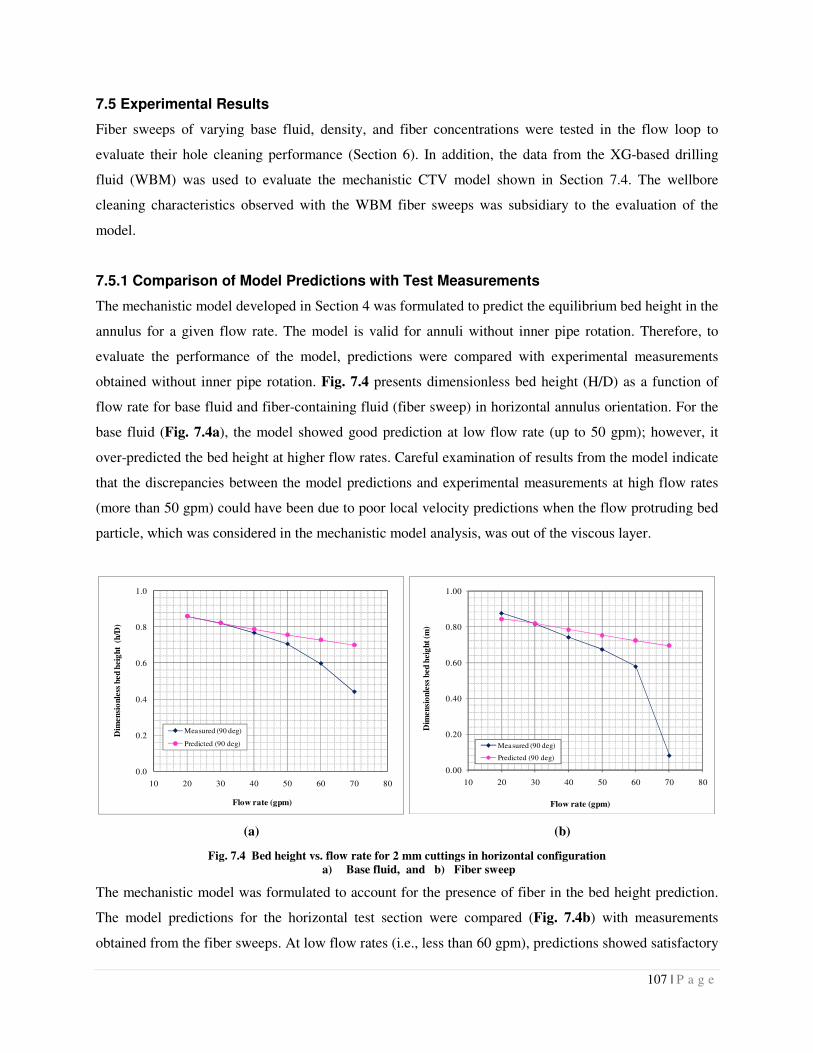
107 | P a g e


Fiber sweeps of varying base fluid, density, and fiber concentrations were tested in the flow loop to

evaluate their hole cleaning performance (Section 6). In addition, the data from the XG-based drilling

fluid (WBM) was used to evaluate the mechanistic CTV model shown in Section 7.4. The wellbore

cleaning characteristics observed with the WBM fiber sweeps was subsidiary to the evaluation of the

model.

7.5.1 Comparison of Model Predictions with Test Measurements

The mechanistic model developed in Section 4 was formulated to predict the equilibrium bed height in the

annulus for a given flow rate. The model is valid for annuli without inner pipe rotation. Therefore, to

evaluate the performance of the model, predictions were compared with experimental measurements

obtained without inner pipe rotation. Fig. 7.4 presents dimensionless bed height (H/D) as a function of

flow rate for base fluid and fiber-containing fluid (fiber sweep) in horizontal annulus orientation. For the

base fluid (Fig. 7.4a), the model showed good prediction at low flow rate (up to 50 gpm); however, it

over-predicted the bed height at higher flow rates. Careful examination of results from the model indicate

that the discrepancies between the model predictions and experimental measurements at high flow rates

(more than 50 gpm) could have been due to poor local velocity predictions when the flow protruding bed

particle, which was considered in the mechanistic model analysis, was out of the viscous layer.

(a)

(b)

Fig. 7.4 Bed height vs. flow rate for 2 mm cuttings in horizontal configuration

a) Base fluid, and b) Fiber sweep

The mechanistic model was formulated to account for the presence of fiber in the bed height prediction.

The model predictions for the horizontal test section were compared (Fig. 7.4b) with measurements

obtained from the fiber sweeps. At low flow rates (i.e., less than 60 gpm), predictions showed satisfactory

0.0

0.2

0.4

0.6

0.8

1.0

10 20 30 40 50 60 70 80

Dim

en

sio

nle

ss b

ed

hei

gh

t (

h/D

)

Flow rate (gpm)

Measured (90 deg)

Predicted (90 deg)

0.00

0.20

0.40

0.60

0.80

1.00

10 20 30 40 50 60 70 80

Dim

en

sio

nle

ss b

ed h

eig

ht

(m)

Flow rate (gpm)

Measured (90 deg)

Predicted (90 deg)

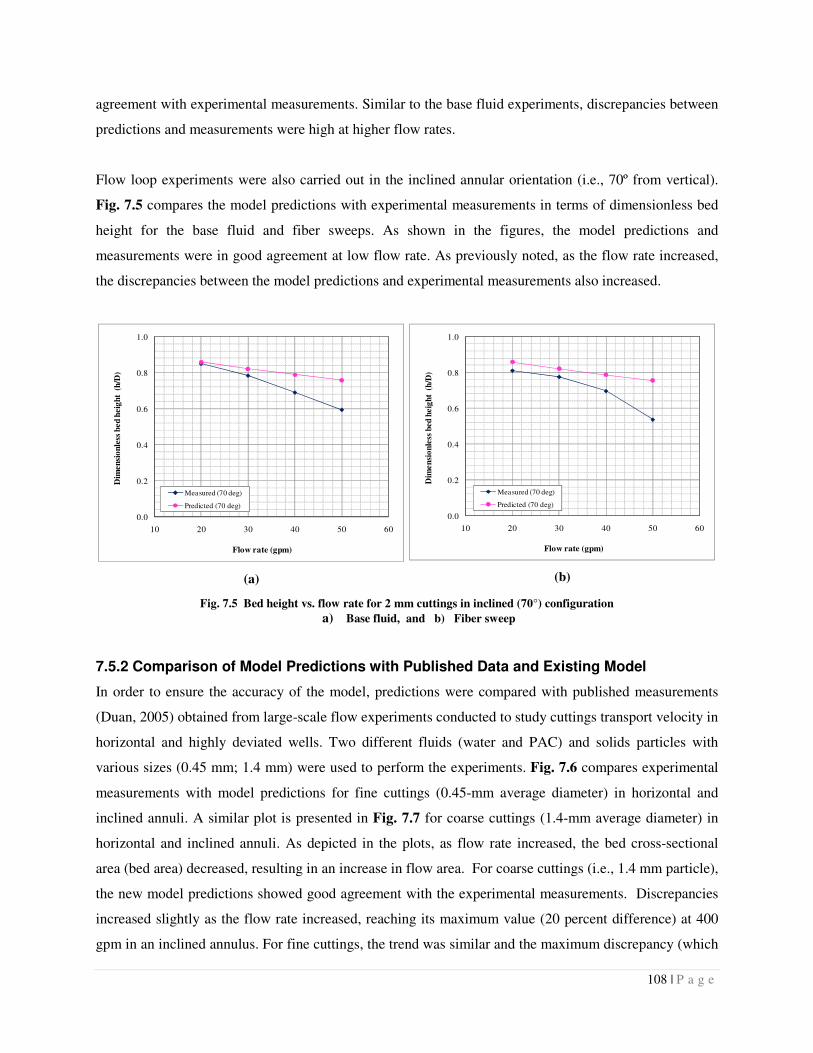
108 | P a g e

agreement with experimental measurements. Similar to the base fluid experiments, discrepancies between

predictions and measurements were high at higher flow rates.

Flow loop experiments were also carried out in the inclined annular orientation (i.e., 70º from vertical).

Fig. 7.5 compares the model predictions with experimental measurements in terms of dimensionless bed

height for the base fluid and fiber sweeps. As shown in the figures, the model predictions and

measurements were in good agreement at low flow rate. As previously noted, as the flow rate increased,

the discrepancies between the model predictions and experimental measurements also increased.

(a)

(b)

Fig. 7.5 Bed height vs. flow rate for 2 mm cuttings in inclined (70°) configuration

a) Base fluid, and b) Fiber sweep

7.5.2 Comparison of Model Predictions with Published Data and Existing Model

In order to ensure the accuracy of the model, predictions were compared with published measurements

(Duan, 2005) obtained from large-scale flow experiments conducted to study cuttings transport velocity in

horizontal and highly deviated wells. Two different fluids (water and PAC) and solids particles with

various sizes (0.45 mm; 1.4 mm) were used to perform the experiments. Fig. 7.6 compares experimental

measurements with model predictions for fine cuttings (0.45-mm average diameter) in horizontal and

inclined annuli. A similar plot is presented in Fig. 7.7 for coarse cuttings (1.4-mm average diameter) in

horizontal and inclined annuli. As depicted in the plots, as flow rate increased, the bed cross-sectional

area (bed area) decreased, resulting in an increase in flow area. For coarse cuttings (i.e., 1.4 mm particle),

the new model predictions showed good agreement with the experimental measurements. Discrepancies

increased slightly as the flow rate increased, reaching its maximum value (20 percent difference) at 400

gpm in an inclined annulus. For fine cuttings, the trend was similar and the maximum discrepancy (which

0.0

0.2

0.4

0.6

0.8

1.0

10 20 30 40 50 60

Dim

en

sio

nle

ss b

ed

heig

ht

(h

/D)

Flow rate (gpm)

Measured (70 deg)

Predicted (70 deg)

0.0

0.2

0.4

0.6

0.8

1.0

10 20 30 40 50 60

Dim

en

sio

nle

ss b

ed h

eig

ht

(h

/D)

Flow rate (gpm)

Measured (70 deg)

Predicted (70 deg)

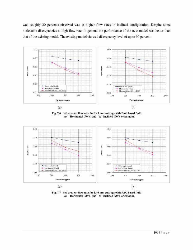
109 | P a g e

was roughly 20 percent) observed was at higher flow rates in inclined configuration. Despite some

noticeable discrepancies at high flow rate, in general the performance of the new model was better than

that of the existing model. The existing model showed discrepancy level of up to 90 percent.

(a)

(b)

Fig. 7.6 Bed area vs. flow rate for 0.45 mm cuttings with PAC based fluid

a) Horizontal (90°), and b) Inclined (70°) orientation

(a)

(b)

Fig. 7.7 Bed area vs. flow rate for 1.40 mm cuttings with PAC based fluid

a) Horizontal (90°), and b) Inclined (70°) orientation

0.00

0.20

0.40

0.60

0.80

1.00

100 200 300 400 500

Ab

ed/A

an

nu

Flow rate (gpm)

Ozbayoglu Model

Mechanistic Model

Measured Data (Duan,2005)

0.00

0.20

0.40

0.60

0.80

1.00

100 200 300 400 500

Ab

ed/A

an

nu

Flow rate (gpm)

Ozbayoglu Model

Mechanistic Model


0.00

0.20

0.40

0.60

0.80

1.00

100 200 300 400 500

Ab

ed/A

an

nu

Flow rate (gpm)

Ozbayoglu Model

Mechanistic Model


0.00

0.20

0.40

0.60

0.80

1.00

100 200 300 400 500

Ab

ed/A

an

nu

Flow rate (gpm)

Ozbayoglu Model

Mechanistic Model


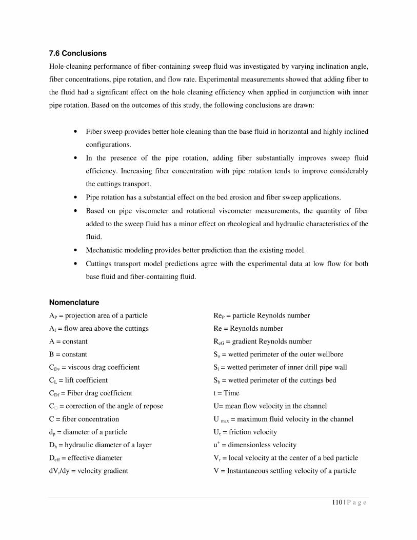
110 | P a g e

7.6 Conclusions

Hole-cleaning performance of fiber-containing sweep fluid was investigated by varying inclination angle,

fiber concentrations, pipe rotation, and flow rate. Experimental measurements showed that adding fiber to

the fluid had a significant effect on the hole cleaning efficiency when applied in conjunction with inner

pipe rotation. Based on the outcomes of this study, the following conclusions are drawn:

• Fiber sweep provides better hole cleaning than the base fluid in horizontal and highly inclined

configurations.

• In the presence of the pipe rotation, adding fiber substantially improves sweep fluid

efficiency. Increasing fiber concentration with pipe rotation tends to improve considerably

the cuttings transport.

• Pipe rotation has a substantial effect on the bed erosion and fiber sweep applications.

• Based on pipe viscometer and rotational viscometer measurements, the quantity of fiber

added to the sweep fluid has a minor effect on rheological and hydraulic characteristics of the

fluid.

• Mechanistic modeling provides better prediction than the existing model.

• Cuttings transport model predictions agree with the experimental data at low flow for both

base fluid and fiber-containing fluid.

Nomenclature

AP = projection area of a particle

Af = flow area above the cuttings

A = constant

B = constant

CDv = viscous drag coefficient

CL = lift coefficient

CDf = Fiber drag coefficient

Cϕ = correction of the angle of repose

C = fiber concentration

dp = diameter of a particle

Dh = hydraulic diameter of a layer

Deff = effective diameter

dVr/dy = velocity gradient

ReP = particle Reynolds number

Re = Reynolds number

ReG = gradient Reynolds number

So = wetted perimeter of the outer wellbore

Si = wetted perimeter of inner drill pipe wall

Sb = wetted perimeter of the cuttings bed

t = Time

U= mean flow velocity in the channel

U max = maximum fluid velocity in the channel

Uτ = friction velocity

u+ = dimensionless velocity

Vr = local velocity at the center of a bed particle

V = Instantaneous settling velocity of a particle

111 | P a g e

dp+ = particle diameter dimensionless

Dr = correction factor of the drag coefficient

Fb = buoyancy force

FD = drag force

FDf = fiber drag force

fbed = friction factor of the bed

FL = lift force

f = friction factor

FDT = total drag force

FDv = viscous drag force

Fg = gravitational force

Fp = plastic force



k' = equivalent consistency index

m = mass of a solids particle

n' = equivalent fluid behavior index


p = pressure

Vs = Terminal settling velocity of a particle

y = vertical distance from the mean bed level

y+ = dimensionless distance

Greek Letters

Гp = rotating torque at point p

ε = pipe roughness

∏ = angle of repose

α = angle of inclination from vertical

α = exponent power of the fiber concentration �� = Shear rate

δ+ = dimensionless of thickness laminar sub-layer


ρf = Fluid density

ρp = density of a particle Ë= kinematic viscosity

τy = yield stress

τbed = average bed shear stress

τw = wall shear stress

τdis = shear stress distribution around a bed particle

References

Ahmed, R.M., Skalle. P. and Johansen. S.T. 2002. A Mechanistic Model to Determine the Critical Flow

Velocity Required to Initiate the Movement of Spherical Bed Particles in Inclined Channels.

Chemical engineering science , 58 (2003) 2153-2163, 4 November.

Ahmed, R.M, Takach, N.E. and Savitri. 2009. Experimental Study on Fiber Sweeps in Horizontal and

Highly Deviated Configurations. Paper SPE 120644 presented at the production operation

Symposium held in Oklahoma city, USA, 4-8 April.

Ahmed, R.M. and Miska, S.Z. 2009. Drilling Hydraulics: Advanced Drilling and Well Technology,

Edited by: Aadnoy, B.; Cooper, I.; Miska, S.; Mitchell, R.F.; Payne, M.L., Society of Petroleum

Engineering, Chap 4.1, 191-220.

112 | P a g e

Bivins, C.H., Bomey, C.V., Fredd, C., Lassek, J., Sullivan, P., Engels, J., Fielder, E. O., Gorham, T.,

Judd, T., Mogollon, A E.S., Tabor, L., Munoz, A. and Willberg, D. 2005. New Fibers for

Hydraulic Fracturing. Oilfield Review, Vol. 17, Issue 2, Schlumberger.

Clark, R.K. and Bickham, K.L. 1994. A Mechanistic Model for Cuttings Transport. Paper SPE presented

at 69th annual technical conference and Exhibition held in New Orleans, La, USA, 25-28

September.

Colebrook, C.F. 1939. Friction Factors for Pipe Flow, Inst. Civil Eng., 11, 133

Dedegil, M.Y. 1987. Drag Coefficient and Settling Velocity of Particles in Non-Newtonian Suspensions.

Journal of fluids engineering, vol. 109/319.

Dodge, D.W. and Metzner, A.B. 1959. Turbulent flow of non-newtonian systems. AIChE Journal, Vol. 5,

No. 2, pp. 189-204.

Duan, M. 2005. An Experimental Study of Small Sand- Size Cuttings Transport in Horizontal and High

Angle Wellbores. The University of Tulsa.

Desouky, S.E.D.M. and Al Saddique, M.A. 1999. Turbulent Pressure Loss of Yield Fluids in Pipes.

Journal of Canadian petroleum technology, Vol. 38, No. 13.

Gerhart, P. M, Gross, R. J., & Hochstein, J. I. (1992). Fundamental of Fluid Mechanics (pp. 480–650).

New York: Addison Wesley Publishing Company.

Guogui, F. 1992. An Experimental Study of Free Settling of cuttings in Newtonian and Non-Newtonian

Drillings Fluids: Drag Coefficient and Settling Velocity. Technical University of Berlin.

Harlen, O.G., Sundararajakumar, R.R. and Koch. D.L. 1999. Numerical Simulations of a Sphere Settling

through a Suspension of Neutrally Buoyant Fibers. J. fluid mech., Vol. 388, pp. 355-388.

Larsen, T.I., Pilehvari, A.A. and Azar. J.J. 1997. Development of a New Cuttings-Transport Model for

High-Angle Wellbore Including Horizontal Wells. SPE drilling & completion, June.

Liang, S.C., Hong. T. and Fan. L.S. 1995. Effect of Particle Arrangements on the Drag Force of a Particle

in the Intermediate Flow Regime. International journal multiphase flow, Vol. 22, No.2, pp.285-

306.

Duan, M., Stefan. M., Mengjiao. Y., Nicholas. T. and Ahmed. R. 2006. Transport of Small Cuttings in

Extended Reach Drilling. Paper SPE 104192 presented at international Oil and Gas conference ,

China , 5-7 December.

Ozbayoglu, M., Saasen, A., Sorgun, M. and Svanes, K. 2007. Estimating Critical Velocity to Prevent Bed

Development for Horizontal-Inclined Wellbores. Paper SPE/IADC 108005 presented at middle

east technology conference and exhibition held in Cairo, Egypt, 22-24 October.

Persen, L. N. (1972). Boundary Layer Theory (pp. 83–130). Trondhiem:Tapir.

113 | P a g e

Rasi, M. 1994. Hole Cleaning in Large, High Angle Wellbore. Paper IADC/SPE 27464 presented at the

drilling conference held in Dallas, Texas, 15-16 February.

Reed. T.D. and Pilehavari. A.A. 1993. A New Model for Laminar, Transitional and Turbulent Flow of

Drilling Muds. Paper SPE 25456 presented at the production operation Symposium held in

Oklahoma city, USA, 21-23 March.

Saffman. P.G. 1964. The Lift on a Small Sphere in a Slow Shear Flow. Journal fluid mechanic, Vol.22,

part 2, pp. 385-400.

White, F. M. (1991). Viscous Fluid Flow (2nd ed .) (pp. 181–200). New York: McGraw-Hill.

RPSEA - National Energy Technology Laboratory library/research/oil-gas/deepwater... · RPSEA FINAL...

Documents

Transcript of RPSEA - National Energy Technology Laboratory library/research/oil-gas/deepwater... · RPSEA FINAL...