Rotordynamic Machines - Durham Universitycommunity.dur.ac.uk/g.l.ingram/download/NLNG2017... ·...

Rotordynamic Machines NLNG Course 2017

Rotordynamic Machines Table of Contents 1 Velocity Vectors and Turbomachinery Definition ..................................................................... 2

1.1 Cycling Example ..................................................................................................................2 1.2 Sailing Example ....................................................................................................................2 1.3 Definition ..............................................................................................................................3 1.4 Understanding Turbomachine Geometry .............................................................................3 1.5 Fundamental Principle ..........................................................................................................4 1.6 Cascade Model ......................................................................................................................5 1.7 Analysis Model .....................................................................................................................6 1.8 Notation Used in the Course .................................................................................................6 1.9 Additional Notes ...................................................................................................................7

1.9.1 Classification .................................................................................................................7 1.9.2 Design Objectives .........................................................................................................7

2 Conservation of Mass, Momentum and Energy ......................................................................... 8 2.1 Continuity (Conservation of Mass) ......................................................................................8

Axial Flow Machines.............................................................................................................8Radial Machines.....................................................................................................................8Centrifugal Machines.............................................................................................................8

2.1.1 Axial Flow Gas Turbine CrossSection ........................................................................9 2.2 Conservation of Angular Momentum .................................................................................10

Turbines and Compressors...................................................................................................10 2.2.1 Implications and Simplifications of the Euler Work Equation ...................................11

2.3 How to draw a Velocity Triangle .......................................................................................11 2.4 Conservation of Energy .....................................................................................................12

2.4.1 Rothalpy: Stator Row ..................................................................................................13 2.4.2 Rothalpy: Rotor Row ..................................................................................................13

3 Efficiency ................................................................................................................................. 15 3.1 Total and Static Conditions ................................................................................................16 3.2 Using Efficiency .................................................................................................................17

4 Reaction and Dimensionless Parameters .................................................................................. 18 4.1 Reaction Definition .............................................................................................................19 4.2 Reaction in Compressors ....................................................................................................20 4.3 Enthalpy Entropy Diagram for a Turbine (For Reference) ................................................20 4.4 Dimensionless Parameters for Turbomachinery .................................................................21

4.4.1 Typical Values of Dimensionless Parameters .............................................................22 4.5 Flow and Stage Loading Coefficient applied to Axial Turbine Stages ..............................22 4.6 Common Design Choices ...................................................................................................23

5 Repeating Stage and Choice of Reaction ................................................................................. 24 5.1 Zero Reaction (Impulse) Stage ...........................................................................................25 5.2 50% Reaction Stage ............................................................................................................25 5.3 Choice of Reaction .............................................................................................................26 5.4 Stage Efficiency ..................................................................................................................27 5.5 Other factors influencing the choice of Reaction ...............................................................28 5.6 A Note on Compressor Design ...........................................................................................29

1


1 Velocity Vectors and Turbomachinery DefinitionVelocity vectors are absolutely fundamental to the understanding of the course. Key Rule:

Absolute Velocity = Relative Velocity + Frame Velocity V= W U

Absolute velocity (V) is the velocity from a stationary reference point.

Relative velocity (W) is the velocity experienced if you were sitting on the moving object.

Frame velocity (U) is the velocity of the moving object.

1.1 Cycling Example

U

1.2 Sailing Example

U

V

Exercise 1: Consider an Office Desk Fan. It rotates at 200 rpm and has a diameter of 30 cm Air enters the fan at 3 m/s, parallel to the axis of rotation. Calculate the relative velocity (W) at the tip of the fan.

2


1.3 DefinitionFeatures:a) Device to exchange mechanical energy with fluid ‘potential energy’ (head or pressure).b) Involves continuously flowing fluid and rotating blades.

From fluid to mechanical energy – pressure or head drop TURBINETo fluid from mechanical energy – pressure or head rise COMPRESSOR, FAN (gases)

PUMP (liquids)Turbomachinery is the generic name for all these machines.

1.4 Understanding Turbomachine GeometryTurbomachinery (usually) hastwo important components: rotor and stator.

Two views are used to show turbomachinery throughout this course:cascade view:

meridional view:

3


1.5 Fundamental PrincipleTorque = Rate of Change of Angular Momentum

Power = Torque Rotational Speed

TURBINE (usually) has stationary blades (also called stator, vanes, nozzles)followed by rotating blades (rotor).

Area decreaseVelocity increasePressure fallsSwirl increases(Angular momentum increase)

Swirl decreasesT= M movement PowerP=T Angular Momentum falls & T in same direction: P = out

(May also get more pressure drop)

COMPRESSOR (usually) Rotor followed by Stator

Rotor increases angular momentumP=T & T opposite, Power INTO fluid

(Usually pressure rise also)

Stator removes swirl (Angular momentum)Area increaseVelocity decreasePressure rise

Generally more difficult to design for rising (adverse) pressure gradient – boundary layers tend to separate high loss.So turbines can do more work for a stage (stator and rotor) than compressors. Turbines can have higher loading per stage. So for given work, need more compressor stages – see jet engine picture.

4


1.6 Cascade ModelIsolated Aerofoil. Consider blade still and air moving with flight velocity, V

Flow for upstream and downstream is the same (e.g. horizontal). Lift reaction acts on an infinite mass of air, so net air deflection is zero.

Cascade Model.Tangential force on finite mass produces net deflection of the flow.

Understanding the cascade model and the meridional view is the most important concept in the entire course. Make sure you fully recognise what is going on here!

5


1.7 Analysis ModelFlow in a real turbomachine is threedimensional, flow varies across blade passage and flow varies up blade span. Even in the flow was totally uniform rotor blade speed varies radially so conditions change up the span! The flow is also unsteady due to relative motion

For Simple Analysis we assume

1. Flow is axisymmetric – ignore variations in circumferential direction (large number blades, very thin).

2. Consider mean stream surface between hub and casing. This is reasonable if hub to casing radius ratio is high – blades are short. However full analysis will have to consider flow at different blade heights.

3. Flow is steady. This turns out to be quite a good assumption you design blades with 90% efficiency using this assumption. Though cutting edge blade design requires thinking about this.

4. Flow follows the blade metal angles. This is actually not true but you will deal with methods to account for this in L4.

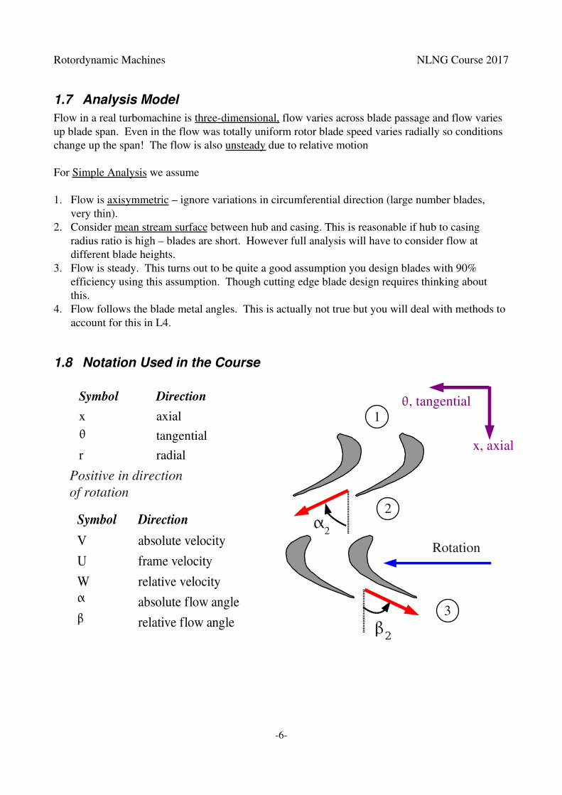
1.8 Notation Used in the Course

Positive in direction of rotation

Symbol Directionx axial tangentialr radial

Rotation

2

2

1

2

3

x, axial

, tangential

Symbol DirectionV absolute velocity U framevelocityW relative velocity absolute flow angle relative flow angle

6


1.9 Additional Notes

1.9.1 ClassificationTurbomachines are generally classified in one of two ways either by type of fluid or by flow direction.

A) Working FluidLiquids – Constant density. Possibility of cavitation if plocal < pvapour pressure poor performance, blade erosion.Gases – Variable density. Possibility of shock waves if Mlocal > 1 Poor performance, blade vibration damage, noise

B) Flow Direction (direction of flow compared to rotational axis)

Axial Machines – Flow roughly along therotational axis

e.g. Jet Engine, Wind Turbine, Fan.

Radial Machine – Flow issubstantially in the radial direction.

The flow may turn from axial to radial (or visa versa).

Often known as centrifugalmachine.

1.9.2 Design ObjectivesThese are the same as most engineering equipment: High efficiency and reliability, low cost, weight, noise, maintenance and pollution. To achieve this, we need to know: a) How does a turbomachine work?b) What are the important performance parameters?c) What affects performance, and how can we estimate it?d) How can we select and design a machine for a given application?This course aims to answer (in part!) the above questions.

7


2 Conservation of Mass, Momentum and EnergyEngineering study of fluid dynamics (and turbomachinery) is built on three sets of equations: 1. Conservation of mass (continuity), 2. Conservation of Momentum and 3. Conservation of Energy.

2.1 Continuity (Conservation of Mass)

m= AV Area and velocity at right angles.

Axial Flow Machines.

Radial Machines

Centrifugal Machinesm1=2 rm1

bV 1x

m2=2 r2 bV 2 r

⇒ rm1b1=r 2b2 ,r 2rm1⇒b2b1

8

If we set V1x ≈ V2r for an incompressible fluid:


Exercise 4: An industrial gas turbine operates at an 8.8:1 pressure ratio and a massflow of 77 kg/s. The exhaust temperature is at 437 degrees centigrade and the inlet temperature to the machine isaround 1000 degrees centigrade. The mean blade radius is 0.4m. The machine is to be designed for a constant axial velocity of 200 m/s.

Estimate the blade heights at entry and exit and sketch the meridional view

2.1.1 Axial Flow Gas Turbine CrossSection

Note: 1). Power output of a turbine stage is much higher than power input of a compressor stage. In terms of Pressure variation along the machine:

2). Overall crosssectional area contracts in compressor part, but expands in the turbine part. In terms of Density variation along the machine:

9


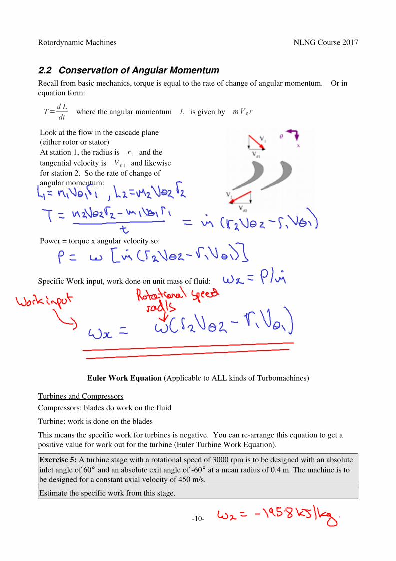
2.2 Conservation of Angular MomentumRecall from basic mechanics, torque is equal to the rate of change of angular momentum. Or in equation form:

T=d Ldt

where the angular momentum L is given by mV r

Look at the flow in the cascade plane (either rotor or stator)At station 1, the radius is r1 and the tangential velocity is V 1 and likewise for station 2. So the rate of change of angular momentum:

Power = torque x angular velocity so:

Specific Work input, work done on unit mass of fluid:

Euler Work Equation (Applicable to ALL kinds of Turbomachines)

Turbines and CompressorsCompressors: blades do work on the fluid

Turbine: work is done on the blades

This means the specific work for turbines is negative. You can rearrange this equation to get a positive value for work out for the turbine (Euler Turbine Work Equation).

Exercise 5: A turbine stage with a rotational speed of 3000 rpm is to be designed with an absolute inlet angle of 60° and an absolute exit angle of 60° at a mean radius of 0.4 m. The machine is to be designed for a constant axial velocity of 450 m/s.

Estimate the specific work from this stage.

10


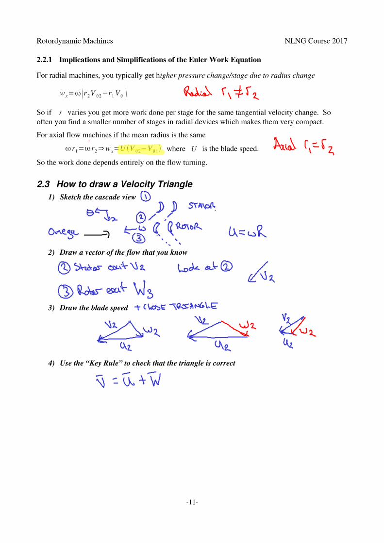
2.2.1 Implications and Simplifications of the Euler Work Equation

For radial machines, you typically get higher pressure change/stage due to radius change

wx=r 2V 2−r1V 1

So if r varies you get more work done per stage for the same tangential velocity change. So often you find a smaller number of stages in radial devices which makes them very compact.

For axial flow machines if the mean radius is the same

r1=r2⇒wx=U V 2−V1 where U is the blade speed.

So the work done depends entirely on the flow turning.

2.3 How to draw a Velocity Triangle1) Sketch the cascade view

2) Draw a vector of the flow that you know

3) Draw the blade speed

4) Use the “Key Rule” to check that the triangle is correct

11


2.4 Conservation of EnergySFEE (L1 Thermo/fluids) between entry (point 1) and exit (point 2) of a turbomachine blade.

QW=m {h2−h112

V 22−V1

2 g z2−z1 }

Ignore height changes:

Divide by mass flow rate:

Where h0 is stagnation enthalpy, total energy change is measured by the change in this quantity.

You will recall the property stagnation pressure: p0=p12

V 2

This is obtained when a fluid is reversibly brought to rest.

There is a similar property stagnation enthalpy: h0=h12V 2

There is also a stagnation temperature: T 0=T 1

2Cp

V 2

Assume negligible heat transfer for turbomachines, i.e. Q=0. This might seem a bit odd as the temperatures inside the machine are quite hot (up to 1800°C or more!) but the velocities through the machine are also very large so the assumption of no heat transfer is quite accurate.

Use wx for work to avoid confusion with relative velocity, so:

Equating with the Euler Work Equation:

So across each blade row (rotor or stator!):

Define Rothalpy, I, as: I=h0−UV

12


Energy conservation (SFEE) is shown in the form of Rothalpy conservation across each blade row:

Rothalpy Conservation (Applicable to rotors, stators in axial and radial turbomachines)

2.4.1 Rothalpy: Stator RowThis is extremely straightforward! For a stator row, U = 0 so:

I=h01=h02 ⇒h1V 1

2

2=h2

V 22

2

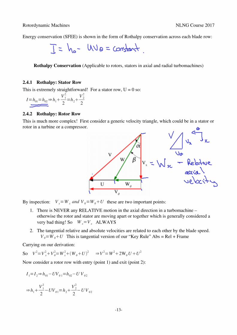
2.4.2 Rothalpy: Rotor RowThis is much more complex! First consider a generic velocity triangle, which could be in a stator orrotor in a turbine or a compressor.

By inspection: V x=W x and V =W U these are two important points:

1. There is NEVER any RELATIVE motion in the axial direction in a turbomachine – otherwise the rotor and stator are moving apart or together which is generally considered a very bad thing! So W x=V x ALWAYS

2. The tangential relative and absolute velocities are related to each other by the blade speed.V =W U This is tangential version of our “Key Rule” Abs = Rel + Frame

Carrying on our derivation:

So V 2=V x2V

2=Wx2W U 2 ⇒V 2=W 22WUU 2

Now consider a rotor row with entry (point 1) and exit (point 2):

I 1=I 2⇒h01−UV 1=h02−U V 2

⇒h1V 1

2

2−UV 1=h2

V 22

2−UV 2

13


Consider LHS:

Substitute for V and V:

Define Relative Stagnation Enthalpy:

Substitute into the above:

Note:1. Axial machines (with little change of, radius): U1=U2

, So Rothalpy conservation is

equivalent to h0rel1=h0rel2

2. Constant relative enthalpy implies no work done in the relative rotor coordinate system, rotor blades do not move in this coordinate system. Energy/work depends on the coordinatesystem. Static Pressure and Temperature do not!

3. Rothalpy is like Enthalpy – a convenient thermodynamic function. You can manage without it but it makes certain things simple! See later in the course on Reaction for example.

Bonus Exercise: Advanced Velocity Triangles.

Most turbomachine parts rotate in the same direction, however it is possible to use contrarotating blades. With a suitably complex arrangement of shafts for power transmission. The photograph on the screen shows several views of a contrarotating fan from the Antonov An70 aircraft.

i) Identify the direction of rotation.

ii) Sketch the meridional and cascade views.

iii) Draw the velocity triangles.

14


3 EfficiencyThere are over one hundred different ways of defining the efficiency of a turbomachine, we will discuss only two of them in this lecture course. Consider a turbine and a compressor on a hs diagram.

Compressor Turbine

Three points are shown on this diagram: 1 the entry condition to the machine, 3 the real exit condition and 3s the isentropic (or ideal) exit condition. (We use 3 rather than 2 as we will considerthe stator/rotor interface as 2 later)

Efficiency can be defined in term of “what you get” divided by “what you pay for”

For a TURBINE, the Isentropic Efficiency is the ratio:Actual Work OutputIdeal Work Output

=wxA

wxI

⇒ it=h3−h1

h3s−h1

The actual is less than the ideal.

For a COMPRESSOR the Isentropic Efficiency is the ratio:Ideal WorkActual Work

=wxI

wxA

⇒ ic=h3s−h1

h3−h1

The actual is greater than the ideal.

Exercise 6. A compressor stage working on air at 1 bar and 25 degrees centigrade has a work inputof 16.81 kJ/kg and an isentropic efficiency of 90%.

Assuming that the air properties are unchanged over the stage calculate the pressure output of the stage.

Fluid properties: R = 287 J/kg K, Cp = 1.01 kJ/kg K, γ=1.4

Hint: For a perfect gas T 3

T1

=( p3

p1)(γ−1)

γand Δh=Cp ΔT

15


3.1 Total and Static ConditionsOne of the reasons there are hundreds of definitions of efficiency is that there are various ways of accounting for the kinetic of the flow at inlet and outlet.

Recall that for each location in a fluid machine there is a static condition and a corresponding stagnation condition. The stagnation condition is the condition that occurs when the fluid is broughtreversibly to rest so the entropy is the same between the static and stagnation conditions.

Consider a turbine stage on the hs diagram: For each condition 1,3,3s there is a corresponding stagnation condition 01,03,03s which is plotted as a vertical line on the hs chart.

ho=hV 2

2By definition, so the vertical length of the line is: V 2

2

Using stagnation conditions allows us to deal with two cases:

1. Where the exit kinetic energy is useful – e.g. for thrust in a jet engine, or subsequent stages in a multistage machine. In this case the energy is not part of the maximum work available.

2. Where the exit kinetic energy is not useful – e.g. the last stage of a steam turbine exhausting to the condenser, or a hydraulic turbine where the water flows away done the exit pipe. An ideal turbine would make use of that exit k.e., so it must be included.

16


Case 1 leads to the isentropic totaltototal efficiency, for a turbine:

it=h01−h03

h01−h03s

Case 2 leads to the isentropic totaltostatic efficiency, for a turbine:

it=h01−h03

h01−h3s

3.2 Using EfficiencyActual efficiencies can be determined by either measurement or by more detailed calculation using computational fluid dynamics (CFD). Though measurement is more reliable at producing absolute values of performance.

The key point is that efficiency provides a link between the work from flow geometry (Euler work equation V ) and actual pressure change delivered or required.

The Euler equation gives you the actual work input/output from the stage. The derivation of the Euler equation takes no account of losses etc in the turbomachine.

For a steam turbine , h1−h3s is obtained from the h – s diagram from the isentropic changep1 to p2

For a turbine using a compressible gas (ideal), using the isentropic relationship:T 3

T1

=( p3

p1)(γ−1)

γ

gives:

w xI=h01−h03S=C pT 011−T 03

T 01 =C pT 011− p03

p01 −1

For incompressible fluid (water or low speed gas flow):

wxI=h01−h03S=v p0=1

p0=g H0

where ΔH0 is the change in total head across the turbine.

Similar relationships exist for a compressor.

Exercise 7. A steam turbine stage operates with inlet stagnation conditions of 120 bar and 500°C, the exit static pressure is 10 bar. If the total to static efficiency of the stage is 90% calculate the specific work output.

17


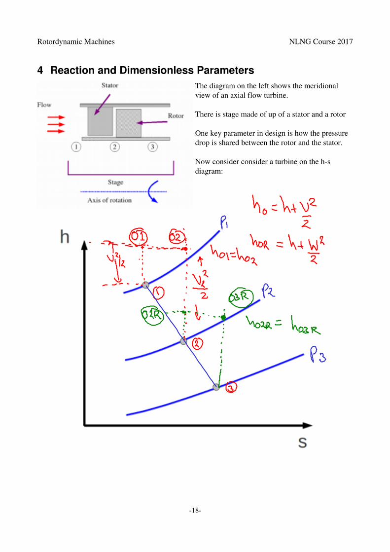
4 Reaction and Dimensionless ParametersThe diagram on the left shows the meridional view of an axial flow turbine.

There is stage made of up of a stator and a rotor

One key parameter in design is how the pressure drop is shared between the rotor and the stator.

Now consider consider a turbine on the hs diagram:

18


There are three key aspects as we build up the diagram:

Stagnation Enthalpy drop in Stator: In the stator h01 = h02 because no work is done in the stator

and h01=h2V 2

2

2⇒h01−h2=

V 22

2similarly

V 12

2=h01−h1

Static Enthalpy drop in the Stator: Note that from the hs diagram it is immediately apparent that:

h01−h2h01−h1⇒V 22V 1

2 and the difference is given by V 2

2

2−V 1

2

2=h1−h2

So there is a static enthalpy drop through the stator due to the acceleration of the flow. No energy isextracted from the stator so there is no stagnation enthalpy drop.

Relative Stagnation Enthalpy: In the rotor (if the flow is axial) there is no change of relative

stagnation enthalpy, h02R=h03R so: W 3

2

2−W 2

2

2=h2−h3

There is a static enthalpy drop through the rotor due to the acceleration of the relative flow.

4.1 Reaction Definition

We define Reaction, R=Static enthalpy drop through rotorStatic enthalpy drop through stage

= hROTOR

hSTAGE

=h2−h3h1−h3

If the flow is reversible, we have:

Tds=dh−1dp=0 , so that dh=

1dp Thus: h≈

1

p ,

or R= hROTOR

hSTAGE

≈ pROTOR

pSTAGE

Thus the reaction is approximately the ratio of the pressure drop across the rotor to that across the stage.

For most turbines: 0.5 > R > 0.050% Reaction, pressure drop shared equally between stator and rotor0%, Zero Reaction (also known as Impulse), all the pressure drop is across the stator.

Exercise 8. Sketch an hs diagram for a 50% and 0% reaction turbine.

19


4.2 Reaction in CompressorsFor Compressors or Pumps, 1 2 is across the rotor so:

R= hROTOR

hSTAGE

=h2−h1

h3−h1≈

pROTOR

pSTAGE

For a compressor minimising the adversepressure gradient is important to avoid boundary layer separation and hence stall and surge.

For a given stage pressure rise the minimum adverse pressure gradient is found with a 50% reaction machine.

For axial compressors, R 50%, the pressure rise is shared equally between rotor and stator. For radial compressors, R > 50%, more pressure rise is across the rotor due to radius increase.

Exercise 9. An industrial gas turbine operates at an 8.8:1 pressure ratio. The turbine exhaustis at 437ºC and the inlet temperature to the turbine is around 1000ºC. The turbine has two equally loaded stages and is designed for a constant axial velocity of 200 m/s. If the entry to the turbine is entirely axial determine the stator exit angle for the first stage if the reaction is 45%.

4.3 Enthalpy Entropy Diagram for a Turbine (For Reference)

20


4.4 Dimensionless Parameters for TurbomachineryThe following dimensionless groups have been found to be very useful in turbomachinery design.

The Flow Coefficient defined as: =V x

Um

This gives the dimensionless flow per unit area compared to the blade speed

The Stage Loading Coefficient: Ψ=wx

Um2=

Δ ho

Um2

This is a measure of work output. Normally we use ∣wx∣ rather than just wx

Reaction : R= hROTOR

hSTAGE

≈ pROTOR

pSTAGE

Efficiency s=h03−h01h03s−h01

Understanding the tradeoffs between these different groups is key to producing successful turbomachinery designs. The figure below shows a number of turbine designs with stage loading and flow coefficient as the axes and efficiency as the contours. This is from Smith (1965) and concerns measurements on the Spey Aircraft Engine.

A number of design choices are hidden by this chart – but it gives an idea of the general tradeoffs inturbomachinery design.

In general the designer of turbomachinery blading does not have complete freedom to determine thedimensionless coefficients that the design will operate at.

For example the mean blade speed is often fixed by mechanical considerations, or the rotation

21


frequency of the machine is fixed by the frequency of the electrical supply and the number of poles in the electrical generator.

The stage loading is often fixed by the number of stages and the required enthalpy drop in the machine.

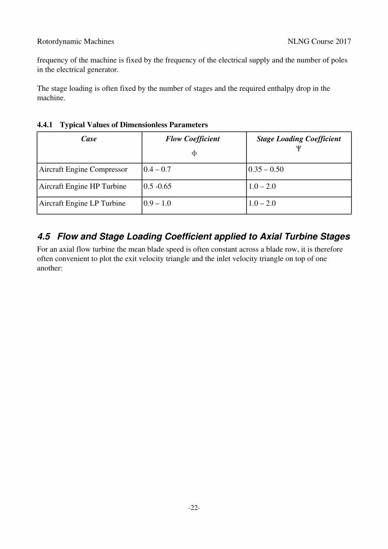
4.4.1 Typical Values of Dimensionless Parameters

Case Flow Coefficient

Stage Loading Coefficient

Aircraft Engine Compressor 0.4 – 0.7 0.35 – 0.50

Aircraft Engine HP Turbine 0.5 0.65 1.0 – 2.0

Aircraft Engine LP Turbine 0.9 – 1.0 1.0 – 2.0

4.5 Flow and Stage Loading Coefficient applied to Axial Turbine StagesFor an axial flow turbine the mean blade speed is often constant across a blade row, it is therefore often convenient to plot the exit velocity triangle and the inlet velocity triangle on top of one another:

22


Now the Euler turbine equation gives:

wx=r 2V 2−r1V 1=Um V

Thus Ψ=wx

Um2=

1Um

ΔV θ

Also =V x

Um

So for a given blade speed, Um: gives the width of the diagram.And for constant axial velocity, Vx: gives the height of the diagram.

Note: Since V =W Um for constant Um then V =W

Exercise 10. Given a turbine blade row with constant axial velocity of 150 m/s at 5000 rpm on a mean radius of 0.7 m and an absolute flow angle at exit from the stator of seventy degrees. Calculate flow coefficient, stage loading coefficient and reaction if the exit flow is axial.

4.6 Common Design ChoicesAs we have alluded to frequently one common design choice is to have constant axial velocity:

V x1=V x2=V x3= constant

There is no fundamental physical law that produces this constraint it is a design choice, although it is often used.

For multistage machines, successive stages are often designed to have identical flow angles and velocities at corresponding positions in each stage:

V 1=V 3⇒ 1=3 and V 1=V 3

This is know as a repeating stage (velocity at inlet = velocity at exit).

Often we design for axial leaving velocity from stage for given V x

Since V 3=V x2V 3

2 V 3 is a minimum when 3=0 , i.e. minimum exit kinetic energy wasted in the last row of blades.

Reference: Smith SF, A simple correlation of turbine efficiency. Journal of Royal Aeronautical Society, Vol. 69, 1965.

23


5 Repeating Stage and Choice of ReactionThe aim of this section is to relate reaction to blade dimensions for a common special case: a repeating stage with constant axial velocity.

Consider the hs diagram opposite,

Δhstage=h1−h3=h01−V 1

2

2 −h03−V 32

2 And this case is for a repeating stage

V 1=V 3

hstage= h0=wx=Um V 2−V 3=UmW 2−W 3

(Recall that V =rW )

hrotor=h2−h3

Earlier we had Rothalpy, I = constant across a rotor row and I=h0−UmVθ=hW 2

2−Um

2

2 so:

h2+W 2

2

2−Um

2

2=h3+

W 32

2−Um

2

2

Rerranging:

h2−h3=12

W 32−W 2

2=12

W 32 V x

2−W 22 −V x

2=12

W 3W 2W 3−W 2

Recall our definition of Reaction R and substitute for h2−h3 and h1−h3 :

R= hrotor

hstage

=h2−h3

h1−h3

=

12

W 3W 2W 3−W 2

Um W 2−W 3=−

12

W 3W 2

Um

We can write W 3=V x tan 3 , and W 2=V x tan2

So R=−12V x

U m

tan2tan3 or

R=−12

tan 2tan 3 (1)

24


Exercise 11. Express reaction for a repeating stage in terms of the absolute stator exit angle and the relative rotor exit angle. A turbine stage of a reaction 0.4 is to operate at a flow coefficient of 1.0. If the stator exit flow angle is 60°. Estimate the rotor relative inlet and exit flow angles.

Following the above exercise:

R=12

−2

tan2tan3 (2)

5.1 Zero Reaction (Impulse) StageIf R = 0, Eqn. (1) tan 2=−tan3 Rotor inlet and outlet equal and opposite: “bucket” shaped blades.

∣W 3∣=∣W 2∣ and β3=−β2 also h2=h3 . So there is no static enthalpy change across rotor.

Since R≈ protor

pstage, no pressure change across rotor: all acceleration of the flow is across the stator.

Note:a) Zero reaction has high turning in rotor – typically β2=60=−β3 ~120 of flow turning in

rotor.b) All the stagnation enthalpy drop must be across the rotor, since only rotor is moving. There can

be no work in the stator as there is force but no distance travelled.

5.2 50% Reaction Stage

Eqn. (2) R=0.5⇒12=12

−2 tanα2tanβ3 After some algebra:

3=−2 and β2=−α3=−α1

So rotor blades are mirror image of stator. 50% reaction gives equal acceleration through rotor and stator, and equal pressure drop.

25


5.3 Choice of Reaction What implications does changing blade design have on loading and performance? Consider a turbine stage with constant axial velocity, repeating stages and an axial exit velocity.

For impulse blades R =0: β3=−β2

So W 2=−W 3 and from the exit velocity triangleV 3=0⇒U=−W 3

So at position 2:V θ2=U+W θ 2=U+U=2U

Euler Equation:wx=U (Vθ3−Vθ 2)=U2×−U=−2U2 take ∣wx∣ :

Ψ=∣wx∣U 2

=2U2

U 2=2

So =2 for impulse blading, repeating stages, constant axial velocity and zero swirl at exit.

For reaction blading R=0.5: stator is mirror of rotor.

We have 2=3=0 and 3=−2

Rotor/stator velocity triangles are a mirror image:

From velocity triangle at 2: V 2=U

From velocity triangle at 3: V 3=0

Euler Equation: wx=U (Vθ3−Vθ 2)=U×−U=−U2

again use ∣wx∣ :

Ψ=∣wx∣U 2

=U2

U2=1

So =1 for 50% reaction blading, repeating stages, constant axial velocity and zero swirl at exit.

V3

Um

W3

W2

Um

V2

Um

Twice the work for Impulse Stage compared to 50% Reaction Stage for the same design constraints.

26


5.4 Stage EfficiencyTurbine efficiency is related to the energy loss or entropy gain within turbomachines. This is an enormously complex topic and the best reference is Denton (1993). There are three basic mechanisms for entropy creation inside a blade row:

1. Viscous friction in either boundary layers or free shear layers.

2. Heat transfer across a finite temperature difference.

3. Nonequilibrium processes such as occur in shock waves.

The latter two are complex subjects and we will leave them aside in this course.

The entropy rise in a boundary layer can be taken to be proportional to a Reynolds number based onboundary layer thickness. In particular for a turbulent boundary layer:

CD=0.0056 Reb−1/6

where Reb=V b

where , are fluid properties and V is the freestream velocity and b

is the boundary layer thickness.

So for a given boundary layer thickness a high freestream velocity will result in greater entropy rise and a lower efficiency.

The peak velocity value in a turbine stage is at stator exit V2.

For: 0% Reaction, Impulse, V 22=V x

2V 2=V x

22U2

50% Reaction V 22=V x

2V 2=V x

2U 2

So for a comparable blade the higher velocity for impulse blading gives more frictional loss and lowers peak efficiency.

27


5.5 Other factors influencing the choice of ReactionTip leakage losses occur at A) stator tip/rotating hub and B) rotor tip/casing clearance

Leakage flow driven by the p across each row which is

linked to reaction as: R≃Δ protor

Δ pstage

For 50% reaction, there is a pressure drop across both the stator and the rotor. So we get some leakage for each row, but the sealing is relatively straightforward. So we can make do with a simple “drum” construction:

For 0% reaction (impulse) all the pressure drop is across stator so the leakage flows would be muchlarger. A “Disc and Diaphragm” construction is often used. Leakage path is at small radius so although p is large the area for flow is reduced, reducing the leakage. However it requires a more complex construction:

28


Gas conditions might influence your choice of reaction. At turbine inlet, temperature and pressure are very high. So it is an advantage to get high work/stage to reduce temperature and pressure quickly:

● Reduce casing stresses● Reduce blade cooling problems

50% Reaction Zero Reaction – ImpulseEqual Δp’s All Δp across stator

Possible adverse (rising) pressure near rotor exit. increased boundary layer loss

High Efficiency, Low Work Output per stage Lower Efficiency, High Work/stage

5.6 A Note on Compressor DesignCompressors operate in an adverse pressure gradient so there is a limit to how much pressure rise you can obtain in a single stage without boundary layer separation.

Moreover for a turbine excursions from design values of or are likely to reduce efficiency, for a compressor they are likely to destroy the performance of the machine.

This means that the design imperative for compressors are about ensuring consistent performance, i.e. avoiding stall and surge rather than achieving maximum efficiency.

Exercise 12.

An intermediate pressure steam turbine is to be designed with 50% reaction stages, constant axial velocity and zero exit swirl. Repeating stages with a stator exit flow angle of 60° are to be used. A mean radius of 0.6 m has been selected and the turbine will be rotated at 3000 rpm. Steam is available at 5 bar, 300 °C and will be exhausted at 1 bar. The turbine is expected to have an efficiency of 90%. The kinetic energy of the flow entering and exiting the turbine and its stages may be ignored.

1) Draw the velocity triangles at entry to the stator, exit from the stator/entry to the rotor and at exitfrom the rotor. Note the key simplifications that the design choices introduce.

2) Demonstrate that nine stages will be sufficient. Steam tables are provided.

3) The tip speed of the machine is limited to 220 m/s. Calculate the steam mass flow and power output from the machine.

Answers to Q3: 48.4 kg/s and 15.26 MW

29

Rotordynamic Machines - Durham Universitycommunity.dur.ac.uk/g.l.ingram/download/NLNG2017... ·...

Documents

Transcript of Rotordynamic Machines - Durham Universitycommunity.dur.ac.uk/g.l.ingram/download/NLNG2017... ·...