Rotordynamic Analysis of Theoretical Models and ...
112
ROTORDYNAMIC ANALYSIS OF THEORETICAL MODELS AND EXPERIMENTAL SYSTEMS A Thesis presented to the Faculty of California Polytechnic State University, San Luis Obispo In Partial Fulfillment of the Requirements for the Degree Master of Science in Mechanical Engineering by Cameron Naugle April 2018
Transcript of Rotordynamic Analysis of Theoretical Models and ...

ROTORDYNAMIC ANALYSIS OF THEORETICAL MODELS AND
EXPERIMENTAL SYSTEMS
A Thesis
presented to
the Faculty of California Polytechnic State University,
San Luis Obispo
In Partial Fulfillment
of the Requirements for the Degree
Master of Science in Mechanical Engineering
by
Cameron Naugle
April 2018

© 2018
Cameron Naugle
ALL RIGHTS RESERVED
ii

COMMITTEE MEMBERSHIP
TITLE: Rotordynamic Analysis of Theoretical
Models and Experimental Systems
AUTHOR: Cameron Naugle
DATE SUBMITTED: April 2018
COMMITTEE CHAIR: Xi (Julia) Wu, Ph.D.
Professor of Mechanical Engineering
COMMITTEE MEMBER: Mohammad Noori, Ph.D.
Professor of Mechanical Engineering
COMMITTEE MEMBER: Peter Schuster, Ph.D.
Professor of Mechanical Engineering
iii

ABSTRACT
Rotordynamic Analysis of Theoretical Models and Experimental Systems
Cameron Naugle
This thesis is intended to provide fundamental information for the construction and
analysis of rotordynamic theoretical models, and their comparison the experimental
systems. Finite Element Method (FEM) is used to construct models using Timo-
shenko beam elements with viscous and hysteretic internal damping. Eigenvalues
and eigenvectors of state space equations are used to perform stability analysis, pro-
duce critical speed maps, and visualize mode shapes. Frequency domain analysis
of theoretical models is used to provide Bode diagrams and in experimental data
full spectrum cascade plots. Experimental and theoretical model analyses are used
to optimize the control algorithm for an Active Magnetic Bearing on an overhung
rotor.
iv

ACKNOWLEDGMENTS
Thanks to:
• Bently Nevada for their support through the Donald E. Bently Center for En-
gineering Innovation at Cal Poly. The equipment provided by Bently Nevada
made this work possible.
• my Advisor, Xi Wu, for always thinking big, and for supporting all my work.
• my family and friends for their support and love.
v

TABLE OF CONTENTS
Page
LIST OF TABLES . . . . . . . . . . . . . . . . . . . . . . . . . . . . . . . . . viii
LIST OF FIGURES . . . . . . . . . . . . . . . . . . . . . . . . . . . . . . . . ix
CHAPTER
1 Vibration Signal Analysis . . . . . . . . . . . . . . . . . . . . . . . . . . . 1
1.1 Data Collection and Processing . . . . . . . . . . . . . . . . . . . . . 1
1.1.1 Amplitude . . . . . . . . . . . . . . . . . . . . . . . . . . . . . 4
1.1.2 Spectrum . . . . . . . . . . . . . . . . . . . . . . . . . . . . . 4
1.1.3 Phase . . . . . . . . . . . . . . . . . . . . . . . . . . . . . . . 6
1.1.3.1 Time Domain Approach . . . . . . . . . . . . . . . . 6
1.1.3.2 Frequency Domain Approach . . . . . . . . . . . . . 7
1.2 Rotordynamic Figures . . . . . . . . . . . . . . . . . . . . . . . . . . 8
1.2.1 Bode . . . . . . . . . . . . . . . . . . . . . . . . . . . . . . . . 8
1.2.2 Full Spectrum and Full Spectrum Cascade . . . . . . . . . . . 10
1.2.3 Orbit . . . . . . . . . . . . . . . . . . . . . . . . . . . . . . . . 11
1.2.4 Filtering . . . . . . . . . . . . . . . . . . . . . . . . . . . . . . 13
1.2.5 Frequency and Time Resolution . . . . . . . . . . . . . . . . . 14
2 Finite Element Method For Rotordynamic systems . . . . . . . . . . . . . 18
2.1 Timoshenko Beam Finite Element . . . . . . . . . . . . . . . . . . . . 18
2.1.1 Kinematic Relationships . . . . . . . . . . . . . . . . . . . . . 19
2.1.2 Internal Constitutive Relationship . . . . . . . . . . . . . . . . 22
2.1.3 Differential Equations of Motion . . . . . . . . . . . . . . . . . 25
2.1.4 Shape Functions . . . . . . . . . . . . . . . . . . . . . . . . . 29
2.1.5 Finite Equations of Motion . . . . . . . . . . . . . . . . . . . . 34
2.1.6 Rotating Internal Damping . . . . . . . . . . . . . . . . . . . 34
2.1.7 Beam Element in Complex Coordinates . . . . . . . . . . . . . 37
2.2 Disk Nodal Equations . . . . . . . . . . . . . . . . . . . . . . . . . . 39
2.2.1 Disk in complex coordinates . . . . . . . . . . . . . . . . . . . 40
2.3 Bearing Nodal Equations . . . . . . . . . . . . . . . . . . . . . . . . . 40
vi

2.3.1 Bearing in Complex Coordinates . . . . . . . . . . . . . . . . 41
2.4 Assembly of the Global System of Equations . . . . . . . . . . . . . . 41
2.4.1 Assembly In the Real Coordinate System . . . . . . . . . . . . 42
2.4.2 In the Complex Coordinate System . . . . . . . . . . . . . . . 42
2.5 Analysis of the Resulting Model . . . . . . . . . . . . . . . . . . . . . 42
3 Frequency Domain Analysis . . . . . . . . . . . . . . . . . . . . . . . . . . 44
3.1 State Space Representation and the Eigenvalue Problem . . . . . . . 45
3.2 Dynamic Response . . . . . . . . . . . . . . . . . . . . . . . . . . . . 47
3.3 Roots Locus and Stability Analysis . . . . . . . . . . . . . . . . . . . 50
3.4 Campbell . . . . . . . . . . . . . . . . . . . . . . . . . . . . . . . . . 53
3.5 Shapes . . . . . . . . . . . . . . . . . . . . . . . . . . . . . . . . . . . 54
4 Synthesis in Example of a Magnetic Bearing on an Overhung Rotor . . . . 58
4.1 Physical System Description . . . . . . . . . . . . . . . . . . . . . . . 58
4.2 Experimental Results . . . . . . . . . . . . . . . . . . . . . . . . . . . 59
4.3 Theoretical Model . . . . . . . . . . . . . . . . . . . . . . . . . . . . . 61
4.3.1 Active Magnetic Bearing . . . . . . . . . . . . . . . . . . . . . 65
4.3.1.1 Proportional Derivative Control . . . . . . . . . . . . 67
4.4 Addition of Magnetic Bearing to the Rotor Model . . . . . . . . . . . 68
5 Conclusion . . . . . . . . . . . . . . . . . . . . . . . . . . . . . . . . . . . . 74
5.1 Summary . . . . . . . . . . . . . . . . . . . . . . . . . . . . . . . . . 74
5.2 Future Work . . . . . . . . . . . . . . . . . . . . . . . . . . . . . . . . 74
BIBLIOGRAPHY . . . . . . . . . . . . . . . . . . . . . . . . . . . . . . . . . 76
APPENDICES
A Bernoulli-Euler Beam equation . . . . . . . . . . . . . . . . . . . . . 79
B RotorFEM MATLAB Code for Constructing and Analyzing FEM Models 82
B.1 Main Object File . . . . . . . . . . . . . . . . . . . . . . . . . . . . . 82
B.2 Matrix Assembly File . . . . . . . . . . . . . . . . . . . . . . . . . . . 82
B.3 Elemental Matrices . . . . . . . . . . . . . . . . . . . . . . . . . . . . 84
B.4 Plotting Functions . . . . . . . . . . . . . . . . . . . . . . . . . . . . 87
C RotorDAQ MATLAB Code for Analyzing Vibration Signals . . . . . 97
C.1 Main Object File . . . . . . . . . . . . . . . . . . . . . . . . . . . . . 97
C.2 Plotting Functions . . . . . . . . . . . . . . . . . . . . . . . . . . . . 101
vii
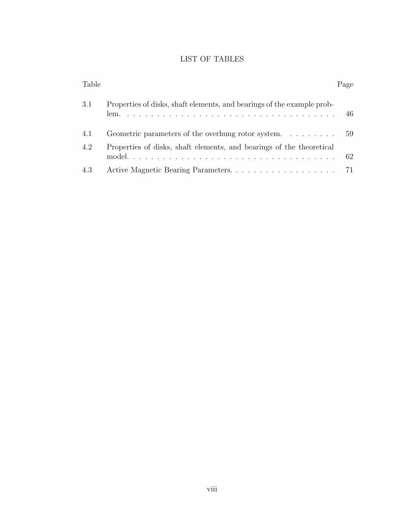
LIST OF TABLES
Table Page
3.1 Properties of disks, shaft elements, and bearings of the example prob-lem. . . . . . . . . . . . . . . . . . . . . . . . . . . . . . . . . . . . 46
4.1 Geometric parameters of the overhung rotor system. . . . . . . . . 59
4.2 Properties of disks, shaft elements, and bearings of the theoreticalmodel. . . . . . . . . . . . . . . . . . . . . . . . . . . . . . . . . . . 62
4.3 Active Magnetic Bearing Parameters. . . . . . . . . . . . . . . . . . 71
viii

LIST OF FIGURES
Figure Page
1.1 Position of the rotor shaft over a period in time. . . . . . . . . . . . 2
1.2 Rotor Spin Speed Windowing effect. . . . . . . . . . . . . . . . . . 3
1.3 A window in time of the transient vibration signals for a window, N ,with nspw of 2048[samples]. . . . . . . . . . . . . . . . . . . . . . . 4
1.4 Bode diagram of the experimental example overhung system. Signalsare filtered to synchronous speed. . . . . . . . . . . . . . . . . . . . 9
1.5 Example Full Spectrum of experimental example system at Ω =1500[RPM]. . . . . . . . . . . . . . . . . . . . . . . . . . . . . . . . 10
1.6 Cascade of the experimental system described in §1.2. . . . . . . . . 11
1.7 3D Orbit of the experimental system described in §1.2. Lighter colorsindicate larger vibration. . . . . . . . . . . . . . . . . . . . . . . . . 12
1.8 Orbits of the experimental example. Spin speed is counterclockwise.Dots indicate the reference position of the shaft, and the beginningof each orbit. . . . . . . . . . . . . . . . . . . . . . . . . . . . . . . 13
1.9 Cascade of the experimental system with a synchronous filter applied. 14
1.10 Cascade of the experimental system with an fres of 0.2[Hz] and aresulting Ωres of 54[RPM]. . . . . . . . . . . . . . . . . . . . . . . . 16
1.11 Cascade of the experimental system with an fres of 2[Hz] and a re-sulting Ωres of 5.5[RPM]. . . . . . . . . . . . . . . . . . . . . . . . . 17
2.1 Timoshenko beam section with degrees of freedom at some point xalong beam axis. . . . . . . . . . . . . . . . . . . . . . . . . . . . . 19
2.2 Beam Element with nodal displacements. . . . . . . . . . . . . . . . 20
2.3 Beam differential element with generalized forces. . . . . . . . . . . 26
2.4 Beam Element with nodal displacements. . . . . . . . . . . . . . . . 30
2.5 Shape Functions as they vary with ζ using two different ratios oflength to radius of beam element. . . . . . . . . . . . . . . . . . . . 33
3.1 Diagram of Two disk model example problem. . . . . . . . . . . . . 45
3.2 Bode diagram of the second disk subject to an unbalance at thesecond disk. Amplitudes of v & w are identical for this asymmetricsystem, phase of w would be lagging v by 90[deg]. . . . . . . . . . . 48
ix

3.3 Nyquist plots for the first two modes at node 6 for the example twodisk problem. . . . . . . . . . . . . . . . . . . . . . . . . . . . . . . 49
3.4 Nyquist Diagram for the first mode at node 6 in the whirl speedrange 1100 < ω < 1300[RPM] at a spin speed, Ω = 4000[RPM].Counter-clockwise path indicates instability. . . . . . . . . . . . . . 49
3.5 Roots Locus of the example problem with an internal damping coef-ficient of 0.0002[s]. . . . . . . . . . . . . . . . . . . . . . . . . . . . 51
3.6 Roots Locus of the example problem in 3-D with an internal dampingcoefficient of 0.0002[s]. . . . . . . . . . . . . . . . . . . . . . . . . . 52
3.7 Stability plot of the example problem. . . . . . . . . . . . . . . . . 53
3.8 Damping ratio of the first three modes of the example problem, withindication of threshold of stability for each mode. . . . . . . . . . . 54
3.9 Campbell Diagram of the example problem. . . . . . . . . . . . . . 55
3.10 Modal shapes of the example problem. . . . . . . . . . . . . . . . . 56
4.1 Overhung rotor system diagram. . . . . . . . . . . . . . . . . . . . 58
4.2 3D Orbit of the experimental overhung rotor system. . . . . . . . . 59
4.3 Cascade of the experimental overhung rotor system. . . . . . . . . . 60
4.4 Bode diagram of the experimental overhung rotor filtered to 1X. . . 61
4.6 Bode Diagram of overhung system without AMB. . . . . . . . . . . 64
4.7 Campbell Diagram of the overhung system without AMB. . . . . . 64
4.8 Roots Locus of overhung system without AMB. . . . . . . . . . . . 65
4.11 Roots locus of Overhung rotor system with varying kv. . . . . . . . 72
4.12 Bode diagram at node 6 comparing the rotor without AMB(solid)and with AMB(dashed). . . . . . . . . . . . . . . . . . . . . . . . . 73
4.13 Bode diagram at node 6 comparing the rotor without AMB(solid)and with AMB(dashed) for complete levitation at node 4. . . . . . 73
A.1 Free body diagram of a beam section in planar bending. . . . . . . 80
x

Chapter 1
VIBRATION SIGNAL ANALYSIS
1.1 Data Collection and Processing
The most important measurement to be made in order to perform significant rotor-
dynamic analysis is the Vibration Signal, V or W . Other important measurements
include Spin Speed, Ω, of the rotating shaft (especially important if during a start-up
or run-down), and a Reference Signal, R, that indicates a rotational position of the
shaft. Orthogonal vibration signals (meaning two independent directions), V & W ,
measuring the position of the shaft centerline can help in characterizing anisotropic
systems. Sampling Rates, fs of the signals mentioned thus far must be high enough
to measure the vibration of interest, typically this is at least several times the highest
expected spin speed of the shaft. It is important to note that these signals can come
from an experiment or a theoretical model. In the case of a theoretical model, the
sampling rate is inversely proportional to the time interval of the differential equation
solver. Or, if a closed form solution exists, the time interval of the time vector chosen
to express the solution within.
There are four variables deduced from the above signals that form the basis for the
majority of rotordynamic figures and analysis. These are: Amplitude of Vibration,
A[m,mils]; Amplitude Spectrum, A(ω)[m,mils]; Phase of Vibration, β[deg, Rad];
and Spin Speed, Ω[Hz,Rad/s,RPM ]. Amplitude Spectrum is actually a two dimen-
sional variable where the variable, ω[Hz,Rad/s,RPM ], represents the Frequency of
Vibration (often called Whirl Speed if its in units of rotation). Figures to be presented
in this work are varying combinations of these four variables. The Bode diagram plots
A against Ω alongside β against Ω. A Spectrum figure plots the absolute value of
1

2 3 4 5 6 7 8
Time [Seconds]
-0.1
-0.05
0
0.05
0.1
Vib
ration S
ignal V
or
W [m
ils]
Figure 1.1: Position of the rotor shaft over a period in time.
A(ω). An extension of this is the Cascade which adds the third dimension of Ω. Orbit
plots represent one cycle of the time domain signals V & W . Lastly, 3D Orbits are
formed by plotting the orbit (V,W ) against Ω. Explanations of the importance and
methods in producing these plots are to follow.
A difficulty to rotordynamic analysis arises in the continuous change of Ω causing a
continuous change in time of its dependent variables A, A(ω), & β. A visualization of
these changes is given in Figure 1.1. This transient nature poses difficulty because the
techniques used to produce A, A(ω), & β from V, W& R rely on a span of subsequent
rotations. A solution to this dilemma utilized in this work is the discretization of
signals V, W, R & Ω into windows in time. Window width will be represented by
the variable nspw[samples] and total number of samples divided by nspw will give
the number of windows in the signals, NW . There is a trade off between resolution
in time, and resolution in frequency of variables as nspw is changed. This trade off
will be elaborated on in §1.2.5.
The windowing approach is visually depicted using Ω in figure 1.2 as it changes
over time. When the width of the window is small enough, such as in Figure 1.2b,
the change in the dependent variable becomes vanishingly small. Other continuous
2

0 50 100
Time (seconds)
15
20
25
30
35
Fre
qu
en
cy o
f R
ota
tio
n (
Hz)
(a) Rotor speed change over time during a
ramp up.
54 54.05 54.1 54.15 54.2
Time (seconds)
20
25
30
Sp
in S
pe
ed
, [H
z]
(b) Rotor speed change over time during a
ramp up.
Figure 1.2: Rotor Spin Speed Windowing effect.
variables such as A, A(ω), & β are expected to behave similarily, in that their value
may be approximated by a single number, or in the case of A(ω) as a single spectrum,
inside the window despite the change in that variable throughout the entire length of
time. The variables V (t), W (t)& R(t) will now take the form V (n), W (n)& R(n)
inside the window (fig. 1.3), where n is sample number. Spin Speed is simply taken as
an average in the window, Ω(N) = avg(Ω(0 : nspw)), where N is the current window
index. Therefore, no further explanation is given for its determination. Amplitude,
Phase, Amplitude Spectrum, and Spin Speed must be calculated in each window, for
a series of windows that cover the entire length of signals. Then a vector of each
variable will exist where the length is equal to the number of windows, NW , and is
given by
NW =length(signals)
nspw
The calculation of each of the variables inside the window, at some N , is given
in the following sections. A useful visual representation of the windowed signals
3

0 200 400 600 800 1000 1200 1400 1600 1800 2000-10
-5
0
5
10
V(n)
W(n)
Figure 1.3: A window in time of the transient vibration signals for awindow, N , with nspw of 2048[samples].
V (n) &W (n) are presented in Figure 1.3 to aid in understanding the sections to
follow.
1.1.1 Amplitude
Amplitude calculation is fairly straightforward within the window. One approach to
calculate the peak to peak amplitude is to take the average over the whole window,
Av(N) = max(V (0 : nspw)) −min(V (0 : nspw)). Another is to use a peak-finding
algorithm to determine the height of each peak and average them all over the sample
length. General computer code packages, such as MATLAB, will contain a peak
finding algorithm, the details of which are out of the scope of this work.
1.1.2 Spectrum
The frequency spectrum of the signal is calculated inside the window using a Fourier
Transform. Influence for this representation of complex amplitude spectrum comes
from [4]. In MATLAB the Fast Fourier Transform (fft) has been preprogrammed
4

allowing easy working between time and frequency domains.
AV (n) =fft(V (n))
nspw, & AW (n) =
fft(W (n))
nspw(1.1)
A useful way to represent the data is using a complex variable to compact the two
orthogonal displacements V & W as
Z(n) = V (n) + iW (n) (1.2)
now the spectrum of this complex value represents both equation planes of vibration
in one equation:
A±(n) =fft(Z(n))
nspw(1.3)
Thus far, the frequency spectrum in the real coordinates and in the complex is in
terms of samples on the independent axis. The frequency vector to which the fft()
corresponds must be calculated–this is the whirl speed, ω. It is known that the slope
of ω is dω = fs/nspw. This value is also called the frequency resolution, fres. It is
also known that the frequency vector is the same length as the time domain signal
f = dω(0 : nspw − 1)
and to center the spectrum at a frequency of 0
Q = ceiling((nspw + 1)/2)
fQ = dω(Q− 1)
ωj = f − fQ
where ωj, here in Hz, is the variable that pairs with the real or complex Ampli-
tude spectrum and the subscript j is a reminder that ω is a discrete variable that
ranges 1 < j < nspw. Now the complex amplitude spectrums can be represented as
AV (ω), AW (ω), & A±(ω). The Amplitude spectrum in real coordinates(1.1) is sym-
metric for positive and negative ω, so typically when the spectrum of a single signal
5

is presented in a spectrum plot or in a cascade it is only on the positive frequency
side. On the other hand, the complex representation of the amplitude spectrum(1.3)
is not symmetric on the positive and negative sides of ω. Understanding why this is
the case stems from realizing the form of the Fourier transform as the summation of
circles in the complex plane, Z(n) =∑j=nspw
j=1 A±(ωj)eiωjt. When ωj is positive this
represents a positive rotation, and when negative represents a negative rotation. For
a given whirl speed, ωj, the positive of that value will be represented by +ω and the
negative as −ω. These two representations of ω correspond to two separate indexes j
as ωj is symmetric about j = nspw/2. This results in the sum of a positively rotating
circle of amplitude, A(+ω) and a negatively rotating circle of amplitude A(−ω). The
ellipse formed by this summation is the orbit of the shaft centerline at this specific
speed[13],[2]. With the understanding of contributions of A(ω) and A(−ω), we realize
that the resulting ellipse will rotate in the counterclockwise direction if A(ω) > A(−ω)
and in the clockwise direction otherwise. This rotation is in reference to the positive
rotation about the z axis defined by the right hand rule from the y-z plane. Since the
same coordinate system is used to represent the sign of Ω, the whirl can be interpreted
as in or opposed to the direction of spin. For a positive Ω, a negative ω corresponds
with an opposing whirl, and vice-versa for a positive ω.
1.1.3 Phase
1.1.3.1 Time Domain Approach
A rather direct way of calculating the phase angle comes from an inspection of the
time domain signal. If some once-per-turn reference is available, then a zero-crossing,
peak-finding, or threshold algorithm can be employed to locate a specific reference
angle of the shaft rotation. In the case that the vibration signal is mostly synchronous
(vibrating at the same frequency as the rotation of the shaft) then a peak-finding or
6

zero-crossing algorithm can be used to determine the number of samples from the shaft
reference angle to the peak of the vibration. Comparison of this sample distance to
the sample distance of an entire cycle of the reference signal will reveal the amount
a signal lags the reference angle as a portion of a full rotation. In terms of samples
this can be represented by the equation
βk = 2π#refk −#peakk#refk −#refk−1
(1.4)
where βk is the phase lag of the signal of interest from the reference signal at the kth
reference cycle, #refk is the sample number of the reference trigger, and #peaki is
the sample number of the peak of the signal of interest. One large advantage to this
brute force method is that it can run continuously and provide phase information
on just the last rotation of the shaft. In the application to the window of vibration
data, fig. 1.3, the measurements of each cycle would be averaged across the window
as β(ω) = avg(βk). This would be done for however many indexes k were found in
the window. In the case of windowed data in Figure 1.3 k = 7[rotations].
1.1.3.2 Frequency Domain Approach
Alternatively, the phase angle can be determined using the frequency domain rep-
resentation of the signals. If the speed of the rotor is known and the time domain
signals V & W are known to be synchronous, or filtered to synchronous, then the
spectrums of the signals of interest can be used to calculate the phase delay. For any
frequency, ω, the angle is calculated using the equation
β(ω) = angle(A(ω))− angle(K(ω))
where, K = fft(K)nspw
is the frequency domain representation of the reference signal.
Either AV , or AW is used to find the phase delay of the V or W time domain vibration
in reference to the once per turn reference of K. It is also possible to find the delay
7

of any time domain signals in reference to any other time domain signal at a specific
frequency using the above equation, though the common practice is to compute the
β angle of both signals and subtract one from another. In synchronous vibration,
ω = Ω.
1.2 Rotordynamic Figures
In the previous section Amplitude, Phase, and Amplitude Spectrum were calculated
for the interior of a window of index N . Each of these variables then need to be
indexed, as all of the windows are processed until the entire signal has been exhausted.
The total number of windows can be realized in the equation NW = length(X)nspw
where X
is a placeholder for any time domain signal. After all windows have been exhausted,
vectors for A(N), β(N) & Ω(N) will all be of length NW , and A(N,ω) is a matrix
of size (NW,nspw).
For visualization of the plots, experimental data from a overhung rotor system,
with one disk supported by two bushings, will used to demonstrate the figures in
use. Data was taken during this experiment with two orthogonal position sensors,
and a reference sensor providing shaft angle and speed information. The experiment
consisted of a ramp-up from 1000[RPM] to 2000[RPM].
1.2.1 Bode
The Bode diagram for the example overhung rotor system is given in Figure 1.4. By
looking at the amplitude portion of the plot it is evident that the V signal undergoes
a natural frequency before the W signal, because the peak for AV occurs before AW .
This idea is also supported through the inspection of the phase lag portion of the plot,
as two seperate transitions are evident. Having two seperate peaks is an indication of
high stiffness anisotropy in the system. By observing the phase lag of each signal, it
8

1000 1200 1400 1600 1800 2000
Spin Speed, [RPM]
0
20
40
Am
plit
ud
e,
A[m
ils]
V
W
1000 1200 1400 1600 1800 2000
Spin Speed, [RPM]
135180225270315
0
Ph
ase
la
g,
[de
g]
Figure 1.4: Bode diagram of the experimental example overhung system.Signals are filtered to synchronous speed.
is evident that the orbit direction is opposite the spin speed between speeds 1280-
1350[RPM]. If normally W lags V with a positive counterclockwise rotation of the
shaft (as is suggested by the phase angles in sub-synchronous and super-synchronous
range), then during the critical speed, the orbit is reversed since V begins to lag W.
Bode diagrams are extremely useful in diagnosing system unbalance through in-
spection of phase lag information. If the shaft was perfectly straight before any
deformation due to rotating unbalance, then the phase lag just before the first natu-
ral frequency is the angle of the unbalance vector. This is due to the fact that before
the first natural frequency, the unbalance vector is aligned with the vibration radially
out from the center of rotation. Furthermore, natural frequencies can be detected
through the use of the phase lag information. Phase lag typically shifts 180[deg] after
completely passing through a natural frequency, and is at 90[deg] during a natural
frequency.
9

-50 -40 -30 -20 -10 0 10 20 30 40 50
2
4
6
8
Figure 1.5: Example Full Spectrum of experimental example system atΩ = 1500[RPM].
1.2.2 Full Spectrum and Full Spectrum Cascade
A single Complex Amplitude Spectrum at a specific speed, A±(1500[RPM ], ω) is
shown as Figure 1.5. This complex representation of the spectrum is referred to as
the “Full Spectrum” of the time domain signal because it contains both positive and
negative frequencies. This figure tells us that the orbit at this speed is in the positive
whirl direction at the dominant frequency, since the positive amplitude, A±(+ω) =
9.13[mils] at its peak is greater than A±(−ω) = 3.47[mils]. Also, there is minimal
amplitude in the spectrum other than this single frequency of ±23.7[Hz] indicating
the vibration is highly synchronous.
A Cascade plot is demonstrated with the experimental system described in §1.2, as
Figure 1.6. Using this figure it is easy to detect the portion of the start-up in which the
orbit is whirling opposite the spin speed. A sharp dip in positive amplitude, A±(ω),
correlated with a sharp rise in negative amplitude, A±(−ω), at around 1320[RPM]
leads to this phenomena.
The Cascade plot is particularly useful in characterizing non-synchronous vibra-
tion. Slightly evident in the example cascade and spectrum of figures 1.6, & 1.5
respectively, is the super-synchronous vibration at twice the spin speed, this is often
10
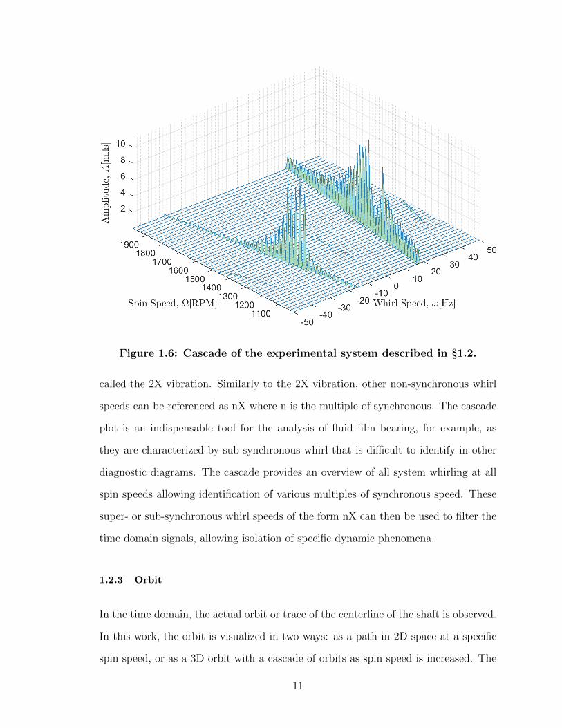
Figure 1.6: Cascade of the experimental system described in §1.2.
called the 2X vibration. Similarly to the 2X vibration, other non-synchronous whirl
speeds can be referenced as nX where n is the multiple of synchronous. The cascade
plot is an indispensable tool for the analysis of fluid film bearing, for example, as
they are characterized by sub-synchronous whirl that is difficult to identify in other
diagnostic diagrams. The cascade provides an overview of all system whirling at all
spin speeds allowing identification of various multiples of synchronous speed. These
super- or sub-synchronous whirl speeds of the form nX can then be used to filter the
time domain signals, allowing isolation of specific dynamic phenomena.
1.2.3 Orbit
In the time domain, the actual orbit or trace of the centerline of the shaft is observed.
In this work, the orbit is visualized in two ways: as a path in 2D space at a specific
spin speed, or as a 3D orbit with a cascade of orbits as spin speed is increased. The
11
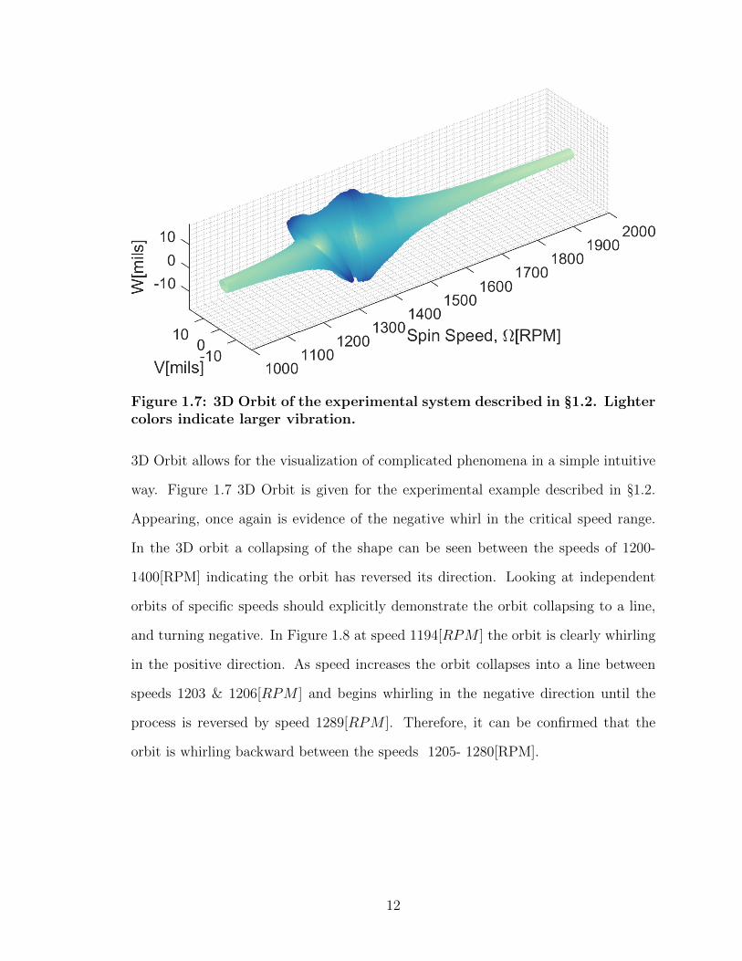
Figure 1.7: 3D Orbit of the experimental system described in §1.2. Lightercolors indicate larger vibration.
3D Orbit allows for the visualization of complicated phenomena in a simple intuitive
way. Figure 1.7 3D Orbit is given for the experimental example described in §1.2.
Appearing, once again is evidence of the negative whirl in the critical speed range.
In the 3D orbit a collapsing of the shape can be seen between the speeds of 1200-
1400[RPM] indicating the orbit has reversed its direction. Looking at independent
orbits of specific speeds should explicitly demonstrate the orbit collapsing to a line,
and turning negative. In Figure 1.8 at speed 1194[RPM ] the orbit is clearly whirling
in the positive direction. As speed increases the orbit collapses into a line between
speeds 1203 & 1206[RPM ] and begins whirling in the negative direction until the
process is reversed by speed 1289[RPM ]. Therefore, it can be confirmed that the
orbit is whirling backward between the speeds 1205- 1280[RPM].
12

−10 0 10
−100
10
Position[mils]
1194[RPM]
−10 0 10
−100
10
Position[mils]
1203[RPM]
−10 0 10
−100
10
Position[mils]
1206[RPM]
−10 0 10
−100
10
Position[mils]
1222[RPM]
−10 0 10
−100
10
Position[mils]
1289[RPM]
Figure 1.8: Orbits of the experimental example. Spin speed is counter-clockwise. Dots indicate the reference position of the shaft, and the be-ginning of each orbit.
1.2.4 Filtering
Correlating phase angles between signals can be extremely difficult due to the noise
and harmonic frequencies that may disrupt the measurement of a phase lag at a
specific frequency. Furthermore, it can be useful to decompose a real signal into
specific harmonic components of the spin speed. One such instance is in the analysis
of a fluid film bearing. Often, the fluid film bearing will cause an unbalance at the
subsynchronous frequency of just under 0.5X. Using a filter, the response of the system
to this specific frequency can be extracted, allowing the analysis of phase angle and
amplitude directly due to the influence of interest.
MATLAB has an extensive library of digital filters that can be adjusted to filter
specific frequency ranges with no phase delay, and recall the states from the previous
window as to not loose dynamic information from one step to the next. Explanation
of filtering in MATLAB has been spared from this work as it is out of the scope.
A synchronous filter was applied the experimental example and the cascade plot
is shown in Figure 1.9. All amplitudes of frequencies other than the synchronous
frequencies have been eliminated. This system did not have strong super- or sub-
synchronous response, so this filtering does not make an appreciable effect to the
13
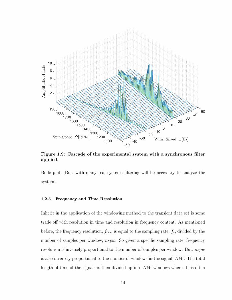
Figure 1.9: Cascade of the experimental system with a synchronous filterapplied.
Bode plot. But, with many real systems filtering will be necessary to analyze the
system.
1.2.5 Frequency and Time Resolution
Inherit in the application of the windowing method to the transient data set is some
trade off with resolution in time and resolution in frequency content. As mentioned
before, the frequency resolution, fres, is equal to the sampling rate, fs, divided by the
number of samples per window, nspw. So given a specific sampling rate, frequency
resolution is inversely proportional to the number of samples per window. But, nspw
is also inversely proportional to the number of windows in the signal, NW . The total
length of time of the signals is then divided up into NW windows where. It is often
14

more convenient in rotordynamics to talk about change in speed instead of time, as
it is more often the independent variable. Total speed range of Ω is divided up into
NW windows, making the speed resolution (the difference in speed from one window
to the next) proportional to NW . Therefore, as NW increases, fres increases, and
Ωres decreases. Where Speed resolution is being referenced here by the variable Ωres.
This relationship is easily explored through the use of the Cascade plot since it
contains both frequency and speed information. An example of a high nspw, low NW ,
low fres, & high Ωres is found in Figure 1.10. The result of low fres, at 0.2[Hz], is
sharp peaks in whirl speed, but since the amplitude spectrum is changing with speed
increase, the spectrum is spread over a large frequency range of Ωres = 54[RPM ].
The opposite condition leading to low Ωres and high fres is presented in Figure 1.11.
In this plot, the fres = 2[Hz] is so high that the whirl speeds are spread over a
large range. On the other hand, the resulting Ωres of 5.5[RPM] provides detailed
information on the effect of changing spin speed. Also, with such high fres a ripple
effect can be seen in the Amplitude spectrum as the actual dominate whirl speed is
between the resolution of 2[Hz] and bleeds into the nearest multiples of 2[Hz]. This
effect is not representative of the actual amplitude spectrum of the signal and is
avoided by choosing a lower fres. The choice of fres is dependent on many factors,
including: fs, spin speed ramp rate, and spin speed range.
15

Figure 1.10: Cascade of the experimental system with an fres of 0.2[Hz]and a resulting Ωres of 54[RPM].
16

Figure 1.11: Cascade of the experimental system with an fres of 2[Hz] anda resulting Ωres of 5.5[RPM].
17

Chapter 2
FINITE ELEMENT METHOD FOR ROTORDYNAMIC SYSTEMS
In this chapter the Finite Element Method(FEM) will be employed in the simulation
of rotordynamic systems. There are many advantages to using this discretized method
to solve problems of rotating machines. One of which is the generic form that the
global equation, and its parts take. The method makes it possible to define all
components of a system separately, only to combine them at the end. Also, FEM
makes it possible to move components around in space without a need to reevaluate
the physics. Finally, the analysis techniques for the resulting equations of motion
are wide-reaching, and will serve to richly enhance our understanding of a complex
system made of simple parts.
First, the beam element commonly refered to as the Timoshenko Beam Element
will be derived from the kinematic and constitutive constraints (derivation of an
alternative element, the Bernoulli-Euler beam element is provided in Appendix A).
The solution to the resulting equation of motion will be discretized and variables
separated in position and time to give the finite element equations of motion. An
extension to the Timoshenko beam element model will be presented that will consider
viscous damping effects in the beam element. Equations for disks, bearings, and
complex versions of all equations will be presented.
2.1 Timoshenko Beam Finite Element
The Timoshenko beam element allows for the beam cross section plane at any axis
location to differ from normal with the axis of the beam. In other words, the element
allows for shear stresses. This element often also includes the effects of rotary inertia
18

u(x, t)
xφ(x, t)
θ(x, t)
v(x, t)
w(x, t)
ψ(x, t)
x
y
z
Figure 2.1: Timoshenko beam section with degrees of freedom at somepoint x along beam axis.
and gyroscopic moments, as it will in this derivation. Generalized displacements used
are assumed to be variable in both time and space. The element has six degrees of
freedom–three translation and three rotations all defined on the beam axis. Beam
displacement coordinates are defined in Figure 2.1. All displacements are functions
of time, t, and the axial spacial coordinate, x. Derivations herein are a synthesis from
references provided in the literature review, further interpretations are adapted from:
[1];[11];[16]. For internal damping interpretations and sources: [6];[15];[9];[7];[23].
2.1.1 Kinematic Relationships
In order to develop the relationship between internal stresses and strains in the beam,
and subsequently the equations of motion, the motion of some arbitrary point on the
beam must be defined in terms of the generalized coordinates. Motion of two points
is taken into consideration to assist in dividing the motion into a translation and a
rotation. These points are shown in Figure 2.2. The first point, C, falls on the beam
axis at location x, and in the undeformed configuration, the vector ~r′c =−→OC forms
a right angle with the surface of the cross section. The second point, P is at some
arbitrary (y, z) location on the cross section. The vecor ~t =−→CP points from the beam
19

y
z
x
C
P
C ′
~rc
P ′
~r
~r′c
~r′
up vp
wp
~ t′
~t
S
S ′
O
Figure 2.2: Beam Element with nodal displacements.
20

axis to the point along the cross section. If we follow this point P we will be able
to define the motion of the cross section as a whole, or more succinctly, to define the
displacements up, vp, wp in terms of the coordinates u, v, w, ψ, θ, & φ. The motion of
point P is split into translation and rotation, where ~t is rotated and ~rc is translated
to point to the deformed location P ′. The vector pointing to P in the undeformed
state is defined as
~r = ~rc + ~t (2.1)
Rotations are represented with a rotation transformation matrix,
~t′ = R~t (2.2)
The linearized first order rotational matrix for small angles is represented by
R =
1 −θ ψ
θ 1 −φ
−ψ φ 1
(2.3)
and the translation with a displacement vector
~r′c = ~rc + ~u (2.4)
Combined motion from P to P ′ can be defined by
~up = ~r′ − ~r (2.5)
where ~up is the vector containing up, vp, &wp. The vector definitions for ~r′ and ~r are
substituted to the above equation to obtain
~up = ~r′c + ~t′ − ~rc + ~t (2.6)
and now using the definition for ~u and ~t′ leads to the simplified expression for the
motion of P
~up = ~u+ (R− I)~t (2.7)
21

expanding matrices reveals the equation
~up =
up
vp
wp
=
u
v
w
+
0 −θ ψ
θ 0 −φ
−ψ φ 0
0
y
z
(2.8)
Therefore, the motion of any point on the beam may be approximated with
~up =
u− θy + ψz
v − φz
w + φy
(2.9)
This equation will be used, in conjunction with material properties, to integrate
over the beam cross sectional area and obtain generalized internal beam forces and
moments.
2.1.2 Internal Constitutive Relationship
Stresses are assumed to exist in the beam in the axial direction, and in shear on
the face of the beam section. Stresses in the transverse, or the y and z, directions
are assumed negligible. Shear stresses out of the plane section are assumed to be
vanishing as the differential element shrinks. Internal damping is to be considered
independently from this material constitutive relationship. Written out, these stresses
are represented by the matrix
σij =
σxx σxy σxz
σxy 0 0
σxz 0 0
(2.10)
Using the Hooke’s Law for a linear elastic isotropic material, expressed as
εij =1
E[(1 + ν)σij − νδijσkk] (2.11)
22

allows the determination of the stress strain relationship in engineering notation asσxx
σxy
σxz
=
E 0 0
0 2G 0
0 0 2G
εxx
εxy
εxz
(2.12)
where, G = E2(1+ν)
. Strains are derived from displacements of equation (2.9) using
a linear strain-displacement relationship for infinitesimal strains: 2εij = ui,j + uj,i.
Non-trivial internal strains areεxx = u′ − θ′y + ψ′z
εxy = 12(v′ − φ′z − θ)
εxz = 12(w′ + φ′y + ψ)
(2.13)
Note that in the case of the Euler-Bernoulli beam derivation the slope in a transverse
direction displacement is equal to the rotation angle about the orthogonal transverse
axis, i.e., v′ = θ and w′ = ψ. Application of those would reduce the system to the
Euler-Bernoulli beam.
It will be proven useful to introduce generalized strains that group strain contri-
butions above as axial, bending, torsion, and shear, represented by the symbols ε, ρ,
ϕ, γ,respectively, as
ε= u′
ρy = −θ′
ρz = ψ′
ϕ= φ′
γy = v′ − θ
γz = w′ + ψ
(2.14)
Plugging in theses new generalized strains in (2.13) givesεxx = ε+ ρyy + ρzz
εxy = 12(γy − ϕz)
εxz = 12(γz + ϕy)
(2.15)
23

Now the stresses in equation (2.12) can be represented with the displacements or the
generalized strains asσxx
σxy
σxz
=
E(u′ − θ′y + ψ′z)
G(v′ − φ′z − θ)
G(w′ + φ′y + ψ)
=
E(ε+ ρyy + ρzz)
G(γy − ϕz)
G(γz + ϕy)
(2.16)
Total strain energy from internal stresses can be expressed by the integral expression
U =
∫V–σijεijdV– (2.17)
and expanded as
U =
∫V–
[σxxεxx + 2σxyεxy + 2σxzεxz] dV– (2.18)
Expand strains using generalized strain expressions (2.15) and collect terms on gen-
eralized strains to get
U =
∫V–
[σxxε+ σxxyρy + σxxzρz + σxyγy + σxzγz + (σxzy − σxyz)ϕ] dV– (2.19)
This internal mechanical energy expression allows us to recognize stresses conjugate
with each generalized strain as the corresponding stress for that phenomena. Integra-
tion allows the determination of the forces and moments related to each generalized
strain as
N =∫AσxxdA = E(Aε+ Syρy + Szρz)
My =∫AσxxzdA = E(Szε+ Ixyρy + Iyρz)
Mz =∫AσxxydA = E(Syε+ Izρy + Ixyρz)
Qy =∫AσxydA = κG(Aγy − Szϕ)
Qz =∫AσxzdA = κG(Aγz + Syϕ)
Mx =∫A
(σxzy − σxyz)dA= κG (Ayγz − Azγy + Jxϕ)
(2.20)
where,
κ = 6(1+ν)7+6ν
, for circular cross sections.
A=∫AdA Sy =
∫AydA
Sz =∫AzdA Iy =
∫Az2dA
Iz =∫Ay2dA Jx= Iy + Iz
24

κ is the shear coefficient which attempts to correct for the fact that the shear strain
is not constant over the beam cross section. Assuming the central axis of the beam
is coincident with the shear center, then Ay = Az = Ixy = 0. Which simplifies the
conjugate forces to
N = EAε = EAu′
My = EIyρz = EIyψ′
Mz = EIzρy = −EIzθ′
Qy = κGAγy = κGA(v′ − θ)
Qz = κGAγz = κGA(w′ + ψ)
Mx = κGJxϕ= κGJxφ′
(2.21)
These forces will be used to evaluate the motion of a beam element using a free body
diagram and resultant motion.
2.1.3 Differential Equations of Motion
The equations of motion will now be derived for the Timoshenko beam element.
External forces are not included in this derivation. Though they may easily be added
to the diagram of figure 2.3 and included in the analysis. It is also assumed that
the cross section remains planar during deformation and the material properties are
homogeneous through time and space. The derivation is the same as for a Euler-
Bernoulli beam with the exception of the constitutive relations used at the end and the
inclusion of torsion and axial degrees of freedom. Using conservation of momentum
and conservation of the moment of momentum a relationship between inertia and
internal forces is developed. Using Figure 2.3 and applying summation of forces in
the x-direction leads to
(N +1
2
∂N
∂xdx)− (N − 1
2
∂N
∂xdx) = ρAdx
∂2u
∂x2(2.22)
25

y
z
x
dx
Ω
N + 12∂N∂xdx
N − 12∂N∂xdx
Mx + 12∂Mx
∂xdx
Mx − 12∂Mx
∂xdx
My + 12
∂My
∂xdx
My − 12
∂My
∂xdx
Mz + 12∂Mz
∂xdx
Qy + 12
∂Qy∂xdx
Qy − 12
∂Qy∂xdx
Mz − 12∂Mz
∂xdx
Qz − 12∂Qz∂xdx
Qz + 12∂Qz∂xdx
Figure 2.3: Beam differential element with generalized forces.
26
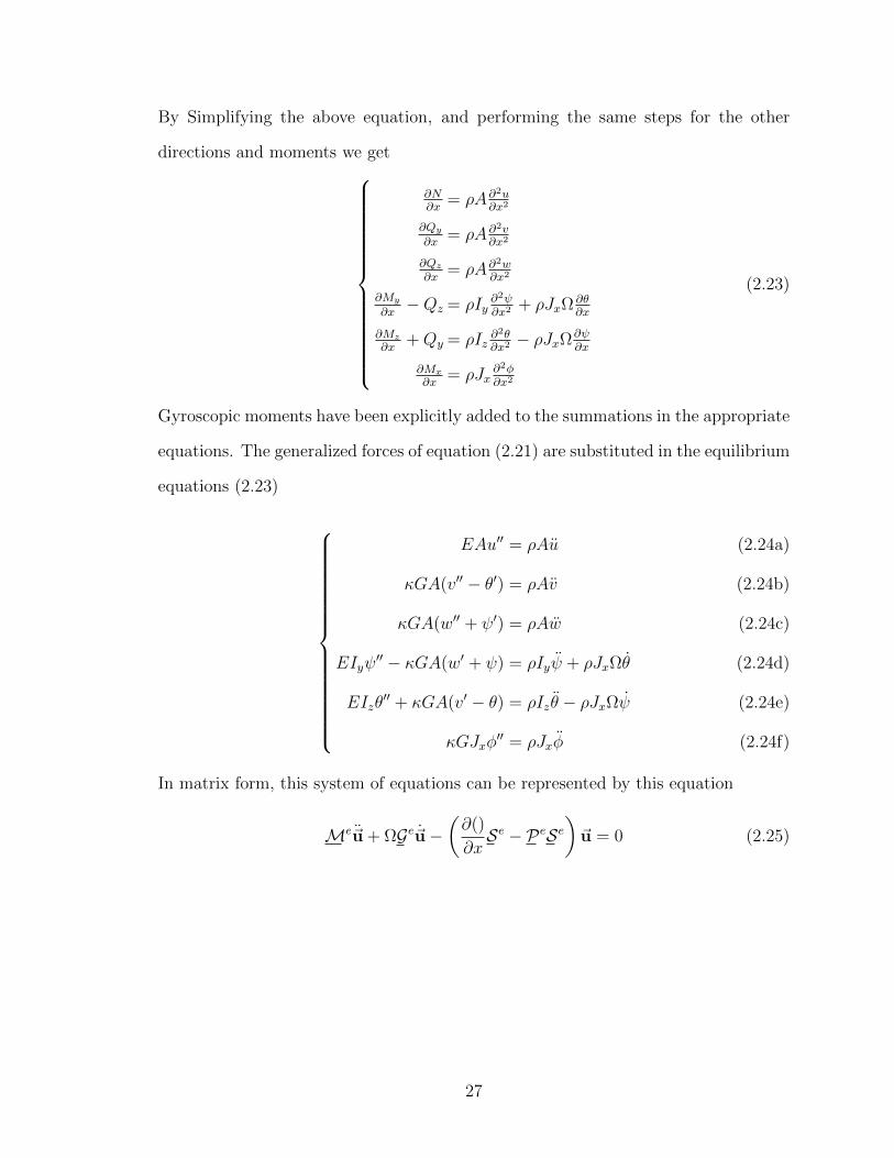
By Simplifying the above equation, and performing the same steps for the other
directions and moments we get
∂N∂x
= ρA∂2u∂x2
∂Qy∂x
= ρA ∂2v∂x2
∂Qz∂x
= ρA∂2w∂x2
∂My
∂x−Qz = ρIy
∂2ψ∂x2
+ ρJxΩ∂θ∂x
∂Mz
∂x+Qy = ρIz
∂2θ∂x2− ρJxΩ∂ψ
∂x
∂Mx
∂x= ρJx
∂2φ∂x2
(2.23)
Gyroscopic moments have been explicitly added to the summations in the appropriate
equations. The generalized forces of equation (2.21) are substituted in the equilibrium
equations (2.23)
EAu′′ = ρAu
κGA(v′′ − θ′) = ρAv
κGA(w′′ + ψ′) = ρAw
EIyψ′′ − κGA(w′ + ψ) = ρIyψ + ρJxΩθ
EIzθ′′ + κGA(v′ − θ) = ρIz θ − ρJxΩψ
κGJxφ′′ = ρJxφ
(2.24a)
(2.24b)
(2.24c)
(2.24d)
(2.24e)
(2.24f)
In matrix form, this system of equations can be represented by this equation
Me~u + ΩGe~u−(∂()
∂xSe − PeSe
)~u = 0 (2.25)
27

where,
Me =
ρA 0 0 0 0 0
0 ρA 0 0 0 0
0 0 ρIy 0 0 0
0 0 0 ρIz 0 0
0 0 0 0 ρA 0
0 0 0 0 0 ρJx
Ge =
0 0 0 0 0 0
0 0 0 0 0 0
0 0 0 ρJx 0 0
0 0 −ρJx 0 0 0
0 0 0 0 0 0
0 0 0 0 0 0
Pe =
0 0 0 0 0 0
0 0 0 0 0 0
0 1 0 0 0 0
−1 0 0 0 0 0
0 0 0 0 0 0
0 0 0 0 0 0
Se =
κGA∂()∂x
0 0 −κGA 0 0
0 κGA∂()∂xκGA 0 0 0
0 0 EIy∂()∂x
0 0 0
0 0 0 EIz∂()∂x
0 0
0 0 0 0 EA∂()∂x
0
0 0 0 0 0 κGJx∂()∂x
(2.26)
and ~u = [v, w, ψ, θ, u, φ]T. The principle of virtual displacements is utilized on the
equations of motion to obtain the weak form of the equations of motion and integrated
over the length of the beam.∫ l
0
δ~uTMe~udx+
∫ l
0
δ~uTΩGe~u−∫ l
0
δ~uT∂()
∂xSe~udx+
∫ l
0
δ~uTPSe~udx = 0 (2.27)
integration by parts on the third term and replacing S with DeB, and making use of
the Identity matrix, I where ∂()∂x
I is interpreted here as if the partial was a scalar∫ l
0
δ~uTMe~udx+ Ω
∫ l
0
δ~uTGe~u +
∫ l
0
δ~uT
(∂()
∂xI + P
)DeB~udx = 0 (2.28)
De =
κGA 0 0 0 0 0
0 κGA 0 0 0 0
0 0 EIy 0 0 0
0 0 0 EIz 0 0
0 0 0 0 EA 0
0 0 0 0 0 κGJx
& B =
∂()∂x
0 0 -1 0 0
0 ∂()∂x
1 0 0 0
0 0 ∂()∂x
0 0 0
0 0 0 ∂()∂x
0 0
0 0 0 0 ∂()∂x
0
0 0 0 0 0 ∂()∂x
(2.29)
Notice that ∂()∂xI + P = BT so the equation of motion becomes∫ l
0
δ~uTMe~udx+ Ω
∫ l
0
δ~uTGe~u +
∫ l
0
δ~uTBTDeB~udx = 0 (2.30)
28

Me is the inertia of the element, Ge is the rotating inertia, De is the material stress-
strain relationship, and Be is the strain-displacement operator. The solution of this
differential system motivates a separation of variables that will be discussed in the
next section.
2.1.4 Shape Functions
The displacements thus far have been assumed to be functions of both position and
time. Now the total displacement is separated into functions that depend on time and
functions that depend on position. This is a fundamental part of the discretization
of the beam element, and the use the finite element method.
~u(x, t) = N(x)~q(t)
~u(x, t) = N(x)~q(t)
~u(x, t) = N(x)~q(t)
δ~u(x, t) = N(x)δ~q(t)
(2.31)
~u = [v, w,−ψ, θ, u, φ]T & ~q = [v1, w1,−ψ1, θ1, v2, w2,−ψ2, θ2, u1, φ1, u2, φ2]T. This
specfic order of ~q is chosen with u and φ at the end to ease the condensation of
the axial and torsional degrees of freedom out of the system if their use is not nec-
essary for the system of interest. ψ angles are defined as negative to allow for the
same stiffness matrix to define the motion in both planes, and more importantly, to
allow for the use of the complex plane to simplify the problem. The shape functions
N(x) interpolate the displacements between the beam ends. These functions must
must solve the static portion of the differential equations (2.24). These shape func-
tions are chosen as a polynomials that satisfy the boundary nodal displacements and
rotations at the ends of a beam element. These nodal degrees of freedom, depicted in
Figure 2.4 are considered to be interpolated through the beam element by the shape
functions. Interpolation functions chosen are listed in Equation (2.32). Axial dis-
29

y
z
u1
φ1
u2
φ2
Ω
θ2
θ1
v1
v2u(x)
xφ(x)
θ(x)
v(x)
w(x)
w2
w1ψ(x)
ψ2
ψ1
l
x
Figure 2.4: Beam Element with nodal displacements.
placement, u, and torsional rotation, φ are independent, so their shape functions are
chosen as polynomials that satisfy the differential equation. Conversely, transverse
displacements, v & w, and bending rotations, ψ & θ are coupled. Coupling of the
shape functions has been proven to reduce some negative effects of linearly interpo-
lated elements [17]. Polynomial functions are chosen for v & w and their rotational
counterparts are derived using the differential relations.
u = c1 + c2x
v = c3 + c4x+ c5x2 + c6x
3
w = c7 + c8x+ c9x2 + c10x
3
φ = c11 + c12x
(2.32a)
(2.32b)
(2.32c)
(2.32d)
c1,2,... are the unknown constants of the polynomial solutions. Using transverse dis-
placement of equations (2.32b) & (2.32c) in the differential equations (2.24b), (2.24c),
30

(2.24d), (2.24e) the interpolation functions of bending rotations are derived as:
ψ = Kyc10 − c8 − 2c9x− 3c10x2
θ = Kzc6 + c4 + 2c5x+ 3c6x2
(2.33a)
(2.33b)
where, Ky = 6EIyκGA
& Kz = 6EIzκGA
.
Boundary conditions for the interpolation polynomials of equations (2.32) & (2.33)
are defined as the components of the vector ~quj = u(xj) and similarily for other
degrees of freedom. Where, j = 1, 2 and defines the two states. In this derivation,
x1 = 0 and x2 = l. Application of these boundary condition results in the below
relationship with the polynomial constants.
u1
u2
v1
v2
w1
w2
ψ1
ψ2
θ1
θ2
φ1
φ2
=
1 0 0 0 0 0 0 0 0 0 0 0
1 l 0 0 0 0 0 0 0 0 0 0
0 0 1 0 0 0 0 0 0 0 0 0
0 0 1 l l2 l3 0 0 0 0 0 0
0 0 0 0 0 0 1 0 0 0 0 0
0 0 0 0 0 0 1 l l2 l3 0 0
0 0 0 0 0 0 0 -1 0 -Ky 0 0
0 0 0 0 0 0 0 -1 -2l -Ky-3l2 0 0
0 0 0 1 0 Kz 0 0 0 0 0 0
0 0 0 1 2l Kz+3l2 0 0 0 0 0 0
0 0 0 0 0 0 0 0 0 0 1 0
0 0 0 0 0 0 0 0 0 0 1 l
c1
c2
c3
c4
c5
c6
c7
c8
c9
c10
c11
c12
(2.34)
Inversion of this matrix results in a system of equations defining the constant c1
through c12. These constants are then substituted in to the polynomial expressions
31

(2.32) & (2.33) giving the interpolations as functions of the nodal displacements as
u = N1u1 +N2u2
v = Tt1yv1 + Tt2yv2 + Tr1yθ1 + Tr2yθ2
w = Tt1zw1 + Tt2ww2 + Tr1zψ1 + Tr2zψ2
ψ = Rt1zw1 +Rt2ww2 +Rr1zψ1 +Rr2zψ2
θ = Rt1yv1 +Rt2yv2 +Rr1yθ1 +Rr2yθ2
φ = N1φ1 +N2φ2
(2.35)
with,
N1 = 1− ζ N2 = ζ
Tt1y,z = 11+αy,z
(2ζ3 − 3ζ2 − αy,zζ + 1 + αy,z) Tt2y,z = 11+αy,z
(−2ζ3 + 3ζ2 + αy,zζ)
Tr1y,z = l1+αy,z
[ζ3 − (2 + 12αy,z)ζ
2 + (1 + 12αy,z)ζ] Tr2y,z = l
1+αy,z[ζ3 − (1− 1
2αy,z)ζ
2 − 12αy,zζ]
Rt1y,z = 6/l1+αy,z
(ζ2 − ζ) Rt2y,z = 6/l1+αy,z
(−ζ2 + ζ)
Rr1y,z = 11+αy,z
(3ζ2 − (4 + αy,z)ζ + 1 + αy,z) Rr2y,z = 11+αy,z
(3ζ2 − (2− αy,z)ζ)
(2.36)
where, αy = 2Ky/l2 = 12EIy
κGAl2, αz = 2Kz/l
2 = 12EIzκGAl2
, & ζ = x/l. (2.35) is expressed in
matrix form as it appears in (2.31) where
N(x) =
Tt1y 0 0 Tr1y Tt2y 0 0 Tr2y 0 0 0 0
0 Tt1z Tr1z 0 0 Tt2z Tr2z 0 0 0 0 0
0 Rt1z Rr1z 0 0 Rt2z Rr2z 0 0 0 0 0
Rt1y 0 0 Rr1y Rt2y 0 0 Rr2y 0 0 0 0
0 0 0 0 0 0 0 0 N1 0 N2 0
0 0 0 0 0 0 0 0 0 N1 0 N2
(2.37)
still with the generalized displacement vector ~q = [v1, w1,−ψ1, θ1, v2, w2,−ψ2, θ2, u1, φ1, u2, φ2]T
Shape functions depend on the term α which is sometimes called the shear cor-
rection factor. This shear correction factor is proportional to the square of the ratio
of radius to length of the beam element. So, as the length increases relative to the
radius, α tends to zero. It will be evident in the following section that as α ap-
proaches zero, the equations of motion approach the equations of the Bernoulli-Euler
32

beam. A spatial representation of the shape functions of equation (2.36) is given in
figure 2.5. Shape functions plotted with respect to the non-dimensional length lend
Tt1 Tr1
Tt2 Tr2
Rt1 Rr1
Rt2 Rr2
(a) length to radius ratio of 100.
Tt1 Tr1
Tt2 Tr2
Rt1 Rr1
Rt2 Rr2
(b) length to radius ratio of 1.
Figure 2.5: Shape Functions as they vary with ζ using two different ratiosof length to radius of beam element.
a visualization to the contribution of each shape function. Shape functions for axial
and torsion are omitted since they are just linear polynomials. Each individual plot
can be interpreted as a transformation from the corresponding input coordinate to
the output. For instance, the first shape function plot is the output of v(x) with an
input of v1 while all other coordinates are zero. The shape makes sense under this
interpretation, as the translation starts at some value, v1 and decreases to zero at the
end since v2 is zero. Also, notice how bending is nearly completely eliminated as the
radius approaches the length as in Figure 2.5b. All shapes the Timoshenko beam will
make in the model results is a linear combination of the shapes shown here.
33

2.1.5 Finite Equations of Motion
To obtain the equations of motion in terms of the generalized coordinates, ~q, dis-
placement variables ~u are replaced with definitions in equation 2.31.∫ l
0
NTδ~qTMeN~qdx+ Ω
∫ l
0
NTδ~qTGeN~qdx+
∫ l
0
NTδ~qTBTDeBN~qdx = 0 (2.38)
Note that ~q is not dependent on x so it, and it’s derivatives, may be pulled out of the
integrals. Define B = BN and substitute in, noting that B interpolates strains from
discrete displacements ~q. The motion equations are then∫ l
0
NTMeNdx~q + Ω
∫ l
0
NTGeNdx~q +
∫ l
0
BTDeBdx~q = 0 (2.39)
Define
Me =
∫ l
0
NTMeNdx
Ge =
∫ l
0
NTGeNdx
Ke =
∫ l
0
BTDeBdx
(2.40a)
(2.40b)
(2.40c)
so that, the general equations of motion for the timoshenko beam element are
Me~q + ΩGe~q + Ke~q = 0 (2.41)
notwithstanding the inclusion of viscous and hysteretic internal damping phenomena.
Derivations, and inclusion of these phenomena in the equations of motion are to be
included in the following section.
2.1.6 Rotating Internal Damping
Rotating damping is the main cause of instability in rotating machines. Non-rotating
damping, such as the damping contributions from bearing supports, introduce a sta-
bilizing effect. But, as rotating damping is dependent on rotation, its direction of
34

force can contribute to destabilization. Typically, friction components such as bear-
ings with shrink fits or oil bearings are responsible for this destabilizing force. Due
to the inherent complexity of modeling loose bearing components, or shrink fit dy-
namics, the analysis of the internal damping in the shaft elements is considered alone
for this work. This will allow for the study of the destabilizing effect in general with-
out requiring too much specificity in design parameters. Inclusion of the rotating
damping effect in this way will allow for the design of components, and geometry of
rotor system, to maximize stability. This stability analysis is only possible with the
inclusion of some destabilizing force, [9],[10],[15],[24].
To motivate understanding of this force a simple derivation is provided with a
rotating damping whose force is proportional to the flex of rate of change of the flex
in the shaft. This is easier to define in the rotating reference frame, as the variables
in this coordinate system directly represent the shaft flex from its neutral position.
The rotating coordinates are located in the same plane as the fixed coordinates, but
they rotate with the shaft speed, Ω. They are angularly displaced from the fixed
coordinates at any point in time by the angle Ωt. The viscous damping in this
rotating coordinate system is defined as
~Fξη = −cr
ξc
ηc
(2.42)
translating this force back to the stationary reference frame requires the rotation
transformation matrix
R =
cos Ωt sin Ωt
− sin Ωt cos Ωt
(2.43)
35

which transforms stationary into rotating coordinates as
ξc
ηc
= R
yc
zc
ξc
ηc
= R
yc
zc
+ R
yc
zc
(2.44)
where,
R = Ω
− sin Ωt cos Ωt
− cos Ωt − sin Ωt
(2.45)
Substituting the second equation in 2.44 for the velocities in 2.42
~Fxy = −cr
yc
zc
− crΩ 0 1
−1 0
yc
zc
(2.46)
From equation (2.46) a dependence on both velocity and position is evident. The
portion dependent on the velocity is inherently stable as pulls opposite the motion.
Conversely, the portion dependent on position cross couples the two displacements.
This causes a destabilizing effect that grows as Ω increases. A net destabilizing force
is produced once the latter portion of the exceeds the former. Without the presence
of other non-rotating damping forces, the system will destabilize.
For the beam element, the constitutive relationship given in [24] is comprised of
both viscous and hysteretic forms of damping, ηv & ηh respectively.
σxx = E
εxx√1 + η2
h
+
(ηv +
ηh
ω√
1 + η2h
)εxx
(2.47)
Through the use of kinematics to obtain strain-displacement relations from the above
constraints, εxx = −r cos (Ω− ω) t∂2R∂x2
εxx = (Ω− ω)r sin (Ω− ω)t∂2R∂x2− r cos (Ω− ω)t ∂
∂t∂2R∂x2
(2.48)
36

and inspection to obtain moment equations, My =∫ 2π
0
∫ a0
[w + r sin Ωt]σxxdr(rd(Ωt))
Mz =∫ 2π
0
∫ a0−[v + r cos Ωt]σxxdr(rd(Ωt))
(2.49)
we can complete a moment bending relationship to be used in the equations of motionMy
Mz
= EI
[ηa Ωηv + ηb
Ωηv + ηb −ηa
]v′′
w′′
+ EI
[ηv 0
0 −ηv
]v′′
w′′
(2.50)
where, ηa = 1+ηh√1+η2h
& ηb = ηh√1+η2h
Using the same strategy followed when solving for the weak form of the beam
differential equations following the Principle of Virtual Displacements starting at
equation (2.27) will reveal the new equations of motion. Then use of a seperation of
variables as defined by equation (2.31) to arrive at the total beam element equations
of motion including internal damping as
Me~q + (ηvKe + ΩGe)~q + [ηaK
e + (Ωηv + ηb)Ce]~q = 0 (2.51)
where,
I =
0 1 0 0 0 0
−1 0 0 0 0 0
0 0 0 1 0 0
0 0 −1 0 0 0
0 0 0 0 0 0
0 0 0 0 0 0
& Ce =
∫ l0BTIDBdx (2.52)
Ce is the “Circulation matrix”, or the skew symmetric stiffness matrix.
2.1.7 Beam Element in Complex Coordinates
Complex coordinates collapse the equations of each plane into one set of equations.
This lends properties to a axisymmetric rotor systems that will be exploited in the
analysis of the model. For the complex analysis in this body of work, the system
is assumed to be axisymmetric and the torsional and axial degrees of freedom are
37
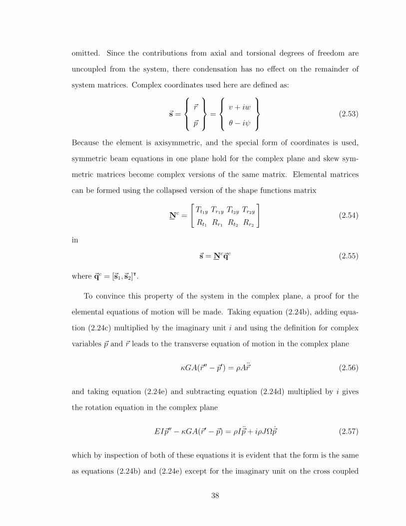
omitted. Since the contributions from axial and torsional degrees of freedom are
uncoupled from the system, there condensation has no effect on the remainder of
system matrices. Complex coordinates used here are defined as:
~s =
~r
~p
=
v + iw
θ − iψ
(2.53)
Because the element is axisymmetric, and the special form of coordinates is used,
symmetric beam equations in one plane hold for the complex plane and skew sym-
metric matrices become complex versions of the same matrix. Elemental matrices
can be formed using the collapsed version of the shape functions matrix
Nc =
[Tt1y Tr1y Tt2y Tr2y
Rt1 Rr1 Rt2 Rr2
](2.54)
in
~s = Nc~qc (2.55)
where ~qc = [~s1,~s2]T.
To convince this property of the system in the complex plane, a proof for the
elemental equations of motion will be made. Taking equation (2.24b), adding equa-
tion (2.24c) multiplied by the imaginary unit i and using the definition for complex
variables ~p and ~r leads to the transverse equation of motion in the complex plane
κGA(~r′′ − ~p′) = ρA~r (2.56)
and taking equation (2.24e) and subtracting equation (2.24d) multiplied by i gives
the rotation equation in the complex plane
EI~p′′ − κGA(~r′ − ~p) = ρI~p+ iρJΩ~p (2.57)
which by inspection of both of these equations it is evident that the form is the same
as equations (2.24b) and (2.24e) except for the imaginary unit on the cross coupled
38

parts of the equation. Now that this idea is motivated, the finite element equations
of motion analogous to equation (2.51) are
Mec~qc + (ηvKec − iΩGec)~qc + [ηaK
ec − i(Ωηv + ηb)Cec]~qc = 0 (2.58)
2.2 Disk Nodal Equations
Since the beam element has been discretized into nodal degrees of freedom, so long
as the locations of disks in the model are chosen to coincide with one of these nodal
locations, the expressions for stiffness and inertia can be directly combined with the
global matrices at that node. The mass element is considered as a body at a point
with inertia, gyroscopic moments, and unbalance considered as external forces.
Md~qk + ΩGd~qk = Ω2~Fd (2.59)
The superscript d in the above equation represents that the matrix or array is for
a disk, and the subscript k on the displacement array indicates the array is only
displacements for a single node, written out as: ~qk = [v, w, ψ, θ, u, φ]T. The matrices
and forcing array of (4.6) are as follows
Md =
ρAl 0 0 0 0 0
0 ρAl 0 0 0 0
0 0 ρIz 0 0 0
0 0 0 ρIy 0 0
0 0 0 0 ρAl 0
0 0 0 0 0 ρJx
G =
0 0 0 0 0 0
0 0 0 0 0 0
0 0 0 ρJx 0 0
0 0 −ρJx 0 0 0
0 0 0 0 0 0
0 0 0 0 0 0
~Fd =
ρAlε cos(Ωt+ δε)
ρAlε sin(Ωt+ δε)
−ρ(Iy − Jx)χ sin(Ωt)
ρ(Iz − Jx)χ cos(Ωt)
0
0
(2.60)
39

Disk unbalance is caused by an eccentricity, or a distance between the axis of
rotation and the center of mass of the disk. Eccentricity is represented here as ε and
is equivalent to that geometric distance. The unbalance moments, third and fourth
equations of ~Fd in (2.60), are caused by the skew angle, χ, which is the angle the
disk major axis forms with the axis of rotation. A more detailed explanation of the
moment function from skew angle can be found in [18]. The major axis is the axis
normal from the disk face from which the polar moment of inertia, Jx is defined.
2.2.1 Disk in complex coordinates
Disk equations of motion (4.6) are converted to the complex plane in the same manner
the beam element was derived in §2.1.7
Mdc~qck − iΩGdc~qck = Ω2~Fdc (2.61)
where,
Mdc =
ρAl 0
0 ρI
, Gdc =
0 0
0 ρJx
, ~Fdc =
ρAlεeiδεeiΩt
ρ(I − Jx)χeiΩt
2.3 Bearing Nodal Equations
Bearings in this work are to be considered massless points of stiffness and damping
acting at a node. Represented by the local equations of motion
Db~qk + Kb~qk = 0 (2.62)
The superscript b indicates the matrix is for a bearing. A simple model for the
stiffness and damping is used. Structural damping of the bearing is considered to
be proportional to the stiffness, Raleigh Damping for the local bearing system. The
40

stiffness matrix is comprised of only transverse stiffness terms, as
Kb =
kyy kyz 0 0 0 0
kzy kzz 0 0 0 0
0 0 0 0 0 0
0 0 0 0 0 0
0 0 0 0 0 0
0 0 0 0 0 0
Db = aKb (2.63)
The stiffness is typically simplified further to represent an orthotropic bearing, where
kyz = kzy = 0 or further yet as a isotropic bearing, where kyz = kzy = 0 & kyy = kzz =
k. Generally, these unknown parameters of stiffness are determined by changing the
values to achieve the correct natural frequencies of the system.
2.3.1 Bearing in Complex Coordinates
Following the same methodology as sections §2.1.7 & §2.2.1, the equation of motion
in the complex plane is
Dbc~qck + Kbc~qck = 0 (2.64)
where,
Kbc =
k 0
0 k
, Dbc = aKbc
k is the isotropic bearing stiffness. It is possible to define the complex system with
anisotropic terms of stiffness, but the complexity added to the system outweighs the
benefit of using the complex plane in the first place.
2.4 Assembly of the Global System of Equations
The matrices in the global system of equations are determined using the direct ap-
proach of taking the summation of the inertia, damping, stiffness, or force at each
degree of freedom.
41

2.4.1 Assembly In the Real Coordinate System
Combining all beam elements, disks, and bearings leads to the following global equa-
tions of motion in real coordinates.
M~q + G~q + K~q = Ω2~F (2.65)
where M = MeG + Mb
G + MdG D = ηvK
eG + ΩGe
G + ΩGdG + Db
G
K = ηaKeG + (Ωηv + ηb)C
eG + Kb
G~F = ~Fd
G
Subscript G indicates the matrix is in the global coordinate system that contains all
of the degrees of freedom. Care must be taken here to associate the correct degrees of
freedom, and recognize that some of the matrices are elemental and others are nodal.
2.4.2 In the Complex Coordinate System
Performing the same summation as in the real coordinate system, but using complex
coordinates results in the following global equations of motion. There are half as many
equations in this expression than in the equivalent expression in real coordinates 2.65.
M~qc + D~qc + K~qc = Ω2~F (2.66)
where, M = MecG + Mdc
G + MbcG D = ηvK
ecG − iΩ(Gec
G + GdcG ) + Dbc
G
K = ηaKecG − i(Ωηv + ηb)C
ecG + Kbc
G~F = ~Fdc
G
2.5 Analysis of the Resulting Model
A benefit of the finite element method is the resulting general linear Ordinary Dif-
ferential Equations (ODEs) that are left to solve in equations (2.65) & (2.66). Many
42

techniques exist to provide frequency and time domain information on the solution
of this system of equations. In their current state, equations (2.65) & (2.66) may be
analyzed using frequency domain analysis techniques to be discussed in §3. On the
other hand, in order to provide time domain solutions, numerical integration of these
ODEs must be conducted. Details of the process of numerical integration is out of the
scope of this work. Resulting time domain solutions of the ODEs for a specific nodal
location can then be processed using the techniques outlined in §1. This time do-
main method of processing the FEM model is vital for analyzing non-linear differential
equations because frequency domain analysis of non-linear differential equations often
produces disjointed results that are difficult to extrapolate useful information from.
Non-linear effects may result from a more detailed model of bearings, anisotropic
beam elements, loose fittings, and many other sources.
43

Chapter 3
FREQUENCY DOMAIN ANALYSIS
Eigenvalues and eigenvectors of equations of motion will be used to provide informa-
tion on the modal content of the system being analyzed. Eigenvalues can provide
information on the natural frequencies, damping, and stability of the modes of vi-
bration. Eigenvectors will be used to describe the shape of each of these modes of
vibration including relative phase information for each nodal location. Frequency
response functions will describe amplitude of response, phase lag of response from
forcing input, and further stability information on modes. Inspiration for the content
in this section came about as a synthesis of content provided on frequency domain
analysis in [4], & [10].
Rotordynamic analyses are often interested in the dependence of the system on
the spin speed Ω. The inclusion of this parameter as a time dependent variable would
make the solutions of the system much more difficult. In this work, the spin speed
is considered to be constant in each operation, taken in a series of operations as the
spin speed is changed. In this way, the effect of spin acceleration is not taken into
account, but the dependence on spin speed is approximated. For the vast majority
of rotordynamic systems this approximation is sufficiently accurate, especially when
considering that it is not a very common neccessity to ramp up quickly in speed.
For a simple critical speed computation, assuming the form of a homogeneous
solution ~q = eiΩt while neglecting all damping and forcing in the equations of motion
will provide the dynamic undamped forced whirling matrix. Exploring the eignevalues
of this equation will give the undamped critical speeds of the system. In the case that
the natural frequencies (whirl speeds) need to be calculated independent of spin speed,
like in the Campbell diagram, a solution of the form ~q = est is assumed so that the
44

L
a
1 2 3 4 5 6 7
ld
dsdd
b
B2
D1
B1
D2
Figure 3.1: Diagram of Two disk model example problem.
spin speed and whirl speed can vary independently. Eigenvalues of this dynamic free
whirling matrix will provide complex numbers of which the real part is proportional to
damping, and the imaginary is damped natural frequencies of the system. Particular
integrals of the form ~q = eiωt & ~q = eiΩt will be assumed to find the frequency
response.
Details of the different analyses to follow will be accompanied by an example
problem to demonstrate the results. The problem of interest is a simple two disk
rotor system depicted in Figure 3.1. The geometry and material properties are listed
in Table 3.1. The rotor is discretized as in figure 3.1 into 6 elements with geometry
of L = 1.8[m], a = .3[m], & b = .6[m] and bearings located at the ends of the shaft.
3.1 State Space Representation and the Eigenvalue Problem
The system can be represented in state space where,
~z = A~z + B~w, ~z =
~q
~q
(3.1)
45
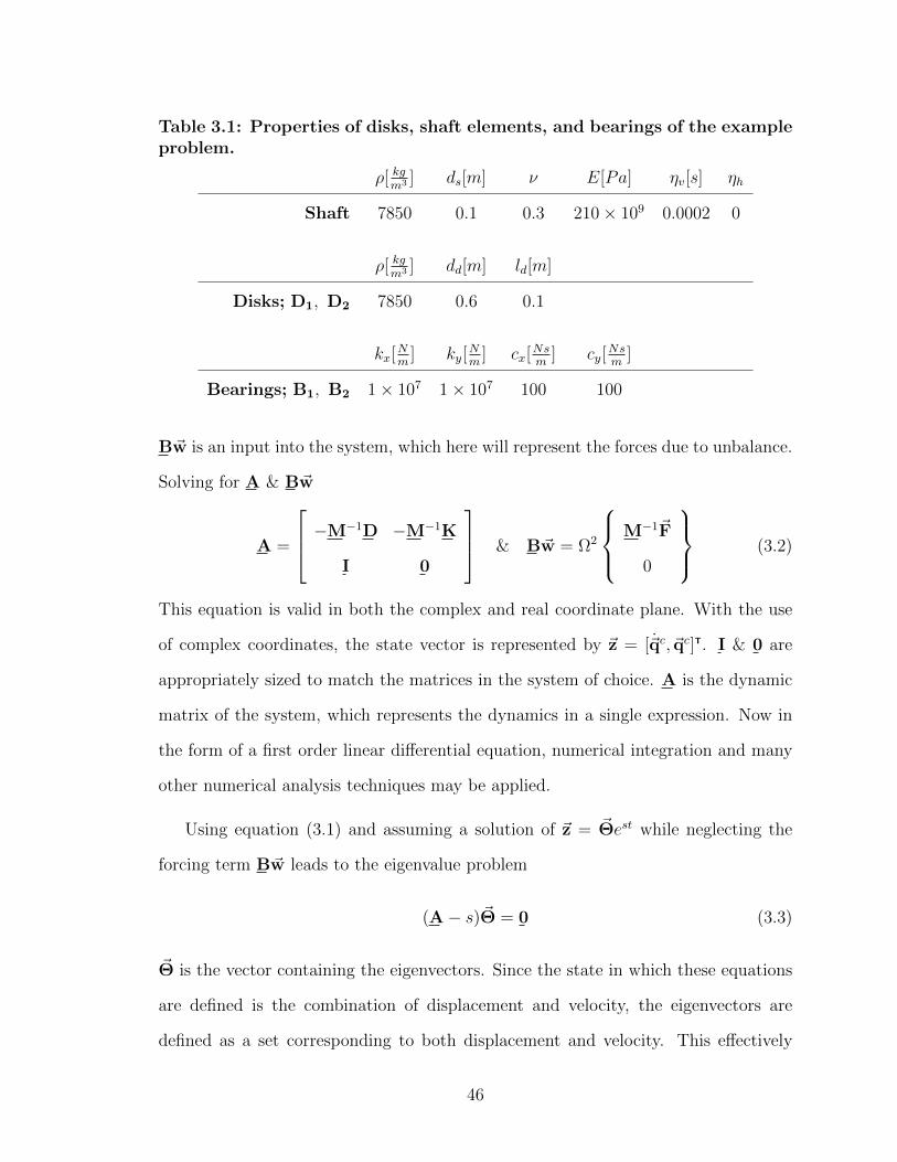
Table 3.1: Properties of disks, shaft elements, and bearings of the exampleproblem.
ρ[ kgm3 ] ds[m] ν E[Pa] ηv[s] ηh
Shaft 7850 0.1 0.3 210× 109 0.0002 0
ρ[ kgm3 ] dd[m] ld[m]
Disks; D1, D2 7850 0.6 0.1
kx[Nm
] ky[Nm
] cx[Nsm
] cy[Nsm
]
Bearings; B1, B2 1× 10⁷ 1× 10⁷ 100 100
B~w is an input into the system, which here will represent the forces due to unbalance.
Solving for A & B~w
A =
−M−1D −M−1K
I 0
& B~w = Ω2
M−1~F
0
(3.2)
This equation is valid in both the complex and real coordinate plane. With the use
of complex coordinates, the state vector is represented by ~z = [~qc, ~qc]T. I & 0 are
appropriately sized to match the matrices in the system of choice. A is the dynamic
matrix of the system, which represents the dynamics in a single expression. Now in
the form of a first order linear differential equation, numerical integration and many
other numerical analysis techniques may be applied.
Using equation (3.1) and assuming a solution of ~z = ~Θest while neglecting the
forcing term B~w leads to the eigenvalue problem
(A− s)~Θ = 0 (3.3)
~Θ is the vector containing the eigenvectors. Since the state in which these equations
are defined is the combination of displacement and velocity, the eigenvectors are
defined as a set corresponding to both displacement and velocity. This effectively
46
duplicates the set as
~Θ =
~θ~q
~θ~q
=
s~θ~q
~θ~q
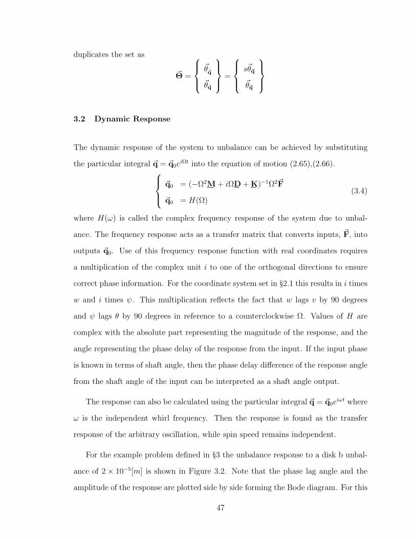
3.2 Dynamic Response
The dynamic response of the system to unbalance can be achieved by substituting
the particular integral ~q = ~q0eiΩt into the equation of motion (2.65),(2.66). ~q0 = (−Ω2M + iΩD + K)−1Ω2~F
~q0 = H(Ω)(3.4)
where H(ω) is called the complex frequency response of the system due to unbal-
ance. The frequency response acts as a transfer matrix that converts inputs, ~F, into
outputs ~q0. Use of this frequency response function with real coordinates requires
a multiplication of the complex unit i to one of the orthogonal directions to ensure
correct phase information. For the coordinate system set in §2.1 this results in i times
w and i times ψ. This multiplication reflects the fact that w lags v by 90 degrees
and ψ lags θ by 90 degrees in reference to a counterclockwise Ω. Values of H are
complex with the absolute part representing the magnitude of the response, and the
angle representing the phase delay of the response from the input. If the input phase
is known in terms of shaft angle, then the phase delay difference of the response angle
from the shaft angle of the input can be interpreted as a shaft angle output.
The response can also be calculated using the particular integral ~q = ~q0eiωt where
ω is the independent whirl frequency. Then the response is found as the transfer
response of the arbitrary oscillation, while spin speed remains independent.
For the example problem defined in §3 the unbalance response to a disk b unbal-
ance of 2× 10⁻⁵[m] is shown in Figure 3.2. Note that the phase lag angle and the
amplitude of the response are plotted side by side forming the Bode diagram. For this
47

0 1,000 2,000 3,000 4,000 5,000 6,000 7,000 8,000-270
-180
-90
0
Speed, Ω[RPM]
Phas
e,β
[deg
]
0 1,000 2,000 3,000 4,000 5,000 6,000 7,000 8,000
10−8
10−6
10−4
Speed, Ω[RPM]
Am
plitu
de,A
[m]
Figure 3.2: Bode diagram of the second disk subject to an unbalance atthe second disk. Amplitudes of v & w are identical for this asymmetricsystem, phase of w would be lagging v by 90[deg].
same set of data, real and imaginary parts of the complex frequency response may
be plotted on the complex plane to form the Nyquist diagram. Figure 3.3 contains
a seperate diagram for each mode. During a natural frequency, if one of the circles
traverses in the counterclockwise direction that mode is deemed unstable. Also, if the
path of one circle crosses the path of the other pertaining to the orthogonal direction,
the whirl is in the negative direction. Using the particular integral of ~q = ~q0eiωt
instead of the synchronous solution, provides whirl frequencies independent of spin
speed. This allows for the investigation of all modes of vibration at a specific spin
speed. For instance, if the spin speed is set to 4000[RPM ] and the Nyquist plot
for the first mode is revisited (Figure 3.4) it is evident that the path traced is in
the counter-clockwise direction indicating instability of mode 1 at the spin speed of
4000[RPM ].
48

−1 0 1
·10−3
−1
−0.5
0
0.5
1·10−3
<(H)
=(H
)
vw
1180
1195ω[RPM ]
(a) Nyquist Diagram for the second mode in the speed range 1180 < Ω < 1195[RPM ].
−2 0 2
·10−4
−2
0
2
·10−4
<(H)
=(H
)
vw
5100
5300
ω[RPM ]
(b) Nyquist Diagram for the second mode in the speed range 5100 < Ω < 5300[RPM ].
Figure 3.3: Nyquist plots for the first two modes at node 6 for the exampletwo disk problem.
1100
1300
ω[RPM ]
−1 0 1
·10−5
−1
0
1
·10−5
<(H)
=(H
)
vw
Figure 3.4: Nyquist Diagram for the first mode at node 6 in the whirl speedrange 1100 < ω < 1300[RPM] at a spin speed, Ω = 4000[RPM]. Counter-clockwise path indicates instability.
49

3.3 Roots Locus and Stability Analysis
One valuable facet of a rotordynamic model is its ability to predict instability. Unsta-
ble operation of rotor systems can lead to failures and unsafe operating conditions.
Before the advent of modern predictive models for rotating machinery, it was not
common to operate a machine above the first critical speed. Internal damping and
other rotating damping can cause a subsynchronous whirl when operating above the
first critical speed, this would often lead to failure of machines. The rotating damp-
ing effect is worse for machines with stiff bending modes, and is often instigated by
loose fittings, shrink fits, and couplings. As mentioned in §2.1.6, the effect of external
rotating damping sources will not be investigated here. Rather, the stability will be
tested by modeling the internal damping of the rotor due to viscous heat production
during loading and unloading of the beam in bending. See §2.1.6 for a more detailed
explanation and derivation.
Roots Locus is the plot of eigenvalues on the <−= plane as some value they are
dependent on changes. In rotordynamic analysis the dependent variable is often the
spin speed Ω. Using the definition of the state space eigenvalue problem set out in
(3.3), the eigenvalues s represent a complex set of which the real part is proportional
to damping and the imaginary is the damped natural frequency. The roots locus is
useful in determining stability of the system, and which mode is responsible for the
instability. Using the eigenvalues s of the eigenvalue problem defined in equation
(3.3) on the example problem defined in §3 a plot of the roots locus can be found
as in figure 3.5. Internal damping coefficient, ηv, is added to the system at the
value of 0.0002[s]. The first three modes are presented with the negative complex
eigenvalue being represented in the positive imaginary axis alongside each positive
mode of vibration. In completely symmetric systems, positive and negative modes
have identical eigenvalues at a spin speed of zero. As the spin speed increases, positive
50

−80 −70 −60 −50 −40 −30 −20 −10 0 10
200
400
600
800
<(s)
=(s)[Rad/s]
Positive Whirl SpeedNegative Whirl Speed
Figure 3.5: Roots Locus of the example problem with an internal dampingcoefficient of 0.0002[s].
modes move in the positive real direction–becoming more unstable. On the other
hand, the negative frequencies move in the negative real direction–becoming more
stable. This phenomena of the positive modes becoming more unstable and the
negative becoming more stable is a general trend, but not a rule, rotating damping
defined in §2.1.6 assists in this trend. It is evident by looking at figure 3.5 that the
system becomes unstable at some point, as many of the eigenvalues are in the positive
real region of the plane. According to the plot, the first and second modes both
become unstable as speed increases. Gyroscopic effects tend to increase the whirl
frequency (imaginary part of eigenvalue) of the positive mode, while the opposite
effect is seen in the negative mode. In general, the effect of non-rotating damping is
to rotate modes in the counter-clockwise direction, at first away from the imaginary
axis, and eventually on to the real axis when the mode becomes over-damped. The
goal of the application of the magnetic bearing in §4 will be to provide enough non-
rotating damping to render as many modes as possible over-damped.
51

−70 −60 −50 −40 −30 −20 −10 0
0
200
400
600
800
0
5,000
<(s)
=(s)
Positive Whirl SpeedNegative Whirl Speed
Figure 3.6: Roots Locus of the example problem in 3-D with an internaldamping coefficient of 0.0002[s].
The Roots Locus for the example problem is also presented in three dimensions
to lend in the understanding of the relationship with spin speed. This can be seen in
Figure 3.6. A direct method of measuring the stability of the system is to observe only
the real part of the eigenvalues of the dynamic matrix as they vary with spin speed.
Since the solution was assumed the be of the form ~z = ~Θest, then the eigenvalues
represent the values of the complex exponent s. Splitting s into its real and complex
components as s = σ+ iωd, and plugging into ~z gives: ~z = ~Θeσ+iωd . By inspection, it
is evident that when the real part is positive, the response will grow without bound–an
unstable system.
Damping is commonly represented as a the ratio of the real part of the eigenvalue
to the natural frequency as
ζ =−σωn
, ωn =√σ2 + ω2
d (3.5)
52
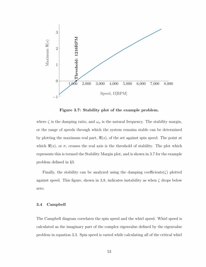
1,000 2,000 3,000 4,000 5,000 6,000 7,000 8,000
−1
0
1
2
3
Thre
shold
:1216R
PM
Speed, Ω[RPM]
Max
imum<
(s)
Figure 3.7: Stability plot of the example problem.
where ζ is the damping ratio, and ωn is the natural frequency. The stability margin,
or the range of speeds through which the system remains stable can be determined
by plotting the maximum real part, <(s), of the set against spin speed. The point at
which <(s), or σ, crosses the real axis is the threshold of stability. The plot which
represents this is termed the Stability Margin plot, and is shown in 3.7 for the example
problem defined in §3.
Finally, the stability can be analyzed using the damping coefficients(ζ) plotted
against speed. This figure, shown in 3.8, indicates instability as when ζ drops below
zero.
3.4 Campbell
The Campbell diagram correlates the spin speed and the whirl speed. Whirl speed is
calculated as the imaginary part of the complex eigenvalue defined by the eigenvalue
problem in equation 3.3. Spin speed is varied while calculating all of the critical whirl
53

1,000 2,000 3,000 4,000 5,000 6,000 7,000 8,0000
0.05
0.1
1216
6081
Speed, Ω[RPM]
Dam
pin
gR
atio
,ζ Negative Whirl Speed
Positive Whirl Speed
Figure 3.8: Damping ratio of the first three modes of the example problem,with indication of threshold of stability for each mode.
speeds at each step of spin speed. The campbell diagram for the example problem
is given in figure 3.9. This diagram can be used to discern the critical speeds of the
system by inspecting where the ω = Ω synchronous line passes through positive and
negative modes in this speed range. Here the synchronous line passes through three
separate modes, each with a positive and negative whirl speed. Note: with the large
influence of the gyroscopic effect in the example problem presented here, the positive
and negative whirl speeds for the second and third modes diverge from one another
rather quickly, but this is not the case for the first mode. A physical interpretation
of this phenomena will be presented in §3.5
3.5 Shapes
Deformed shape of each mode can be predicted using the eigenvectors of the eigenvalue
problem from equation 3.3. Eigenvectors contain displacement arrangement that
corresponds to a natural frequency; this includes phase and relative amplitude of
the generalized displacements from one another. A simple model will be utilized to
conceptualize this idea, consider a rigid rod that can only translate in one direction at
each end. The eigenvectors will contain all linearly independent combinations of the
54

0 1,000 2,000 3,000 4,000 5,000 6,000 7,000 8,0000
2,000
4,000
6,000
8,000
Spin speed Ω[RPM]
Whir
lsp
eed,ωd
[RPM
]
Negative Whirl SpeedPositive Whirl SpeedSynchronous ω = Ω
Figure 3.9: Campbell Diagram of the example problem.
movement of the left side relative to the right. This would be in general; opposite left
and right (i.e. one up, one down), and same left and right(i.e. both up, or both down).
The bending modes of the beam operate in a similar manner but scaled up, and just
like in the simple case, including the same number of modes as there are degrees of
freedom in the system. Since the state space representation used for eigenanalysis
contains ~q, & ~q the eigenvector will contain 2N modes. For a general ith mode
of vibration, the eigenvector ~Θi contains the displacement information. But, since
the portion of ~Θi pertaining to velocities, ~θ~qi, is a linear combination of ~θ~qi, all of
the information is contained in one of these arrays. Therefore, the interpolation of
displacements for the ith mode is given by
~ui = N~θ~qi (3.6)
where, the value of ~ui is now a function of x. So, through the choice of an array of
positions that span the length of the beam element the displacement, and phase angle
distribution of the ith mode of vibration is determined. Amplitude in eah direction is
55
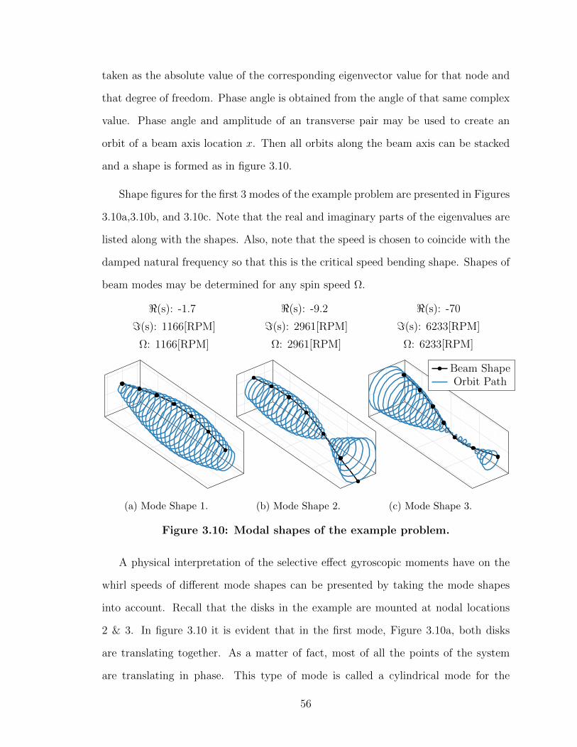
taken as the absolute value of the corresponding eigenvector value for that node and
that degree of freedom. Phase angle is obtained from the angle of that same complex
value. Phase angle and amplitude of an transverse pair may be used to create an
orbit of a beam axis location x. Then all orbits along the beam axis can be stacked
and a shape is formed as in figure 3.10.
Shape figures for the first 3 modes of the example problem are presented in Figures
3.10a,3.10b, and 3.10c. Note that the real and imaginary parts of the eigenvalues are
listed along with the shapes. Also, note that the speed is chosen to coincide with the
damped natural frequency so that this is the critical speed bending shape. Shapes of
beam modes may be determined for any spin speed Ω.
<(s): -1.7
=(s): 1166[RPM]
Ω: 1166[RPM]
(a) Mode Shape 1.
<(s): -9.2
=(s): 2961[RPM]
Ω: 2961[RPM]
(b) Mode Shape 2.
<(s): -70
=(s): 6233[RPM]
Ω: 6233[RPM]
Beam ShapeOrbit Path
(c) Mode Shape 3.
Figure 3.10: Modal shapes of the example problem.
A physical interpretation of the selective effect gyroscopic moments have on the
whirl speeds of different mode shapes can be presented by taking the mode shapes
into account. Recall that the disks in the example are mounted at nodal locations
2 & 3. In figure 3.10 it is evident that in the first mode, Figure 3.10a, both disks
are translating together. As a matter of fact, most of all the points of the system
are translating in phase. This type of mode is called a cylindrical mode for the
56
fact that as the shaft’s path is traced, as it is in 3.10a, it forms a cylinder. The
consequence of this type of motion is small transverse rotation angles, ψ & θ, of
the mass elements. Since the gyroscopic moments are proportional to these angles,
their magnitude is very low compared to transverse effects and as a result the whirl
speeds are nearly unaffected by spin speed changes. On the contrary, modes 2 & 3
of figures 3.10b & 3.10c respectively, the angle of the disks and other mass elements
is changing significantly through rotation. Because of this, large gyroscopic moments
induce an out of phase force that stiffens positive whirl and softens negative whirl
tendencies. Gyroscopic moments are larger in these types of modes where there is a
point of inflection on the beam, commonly called an antinode of vibration. This mode
is called a conical mode because the shape of the path forms one or many cones.
57

Chapter 4
SYNTHESIS IN EXAMPLE OF A MAGNETIC BEARING ON AN OVERHUNG
ROTOR
Analysis and modeling techniques of the previous chapters will now be put to use in a
practical example. The goal of which will be to reduce vibration on an overhung disk
rotor system with the use of an Active Magnetic Bearing(AMB). An experimental
test rig, not unlike the system used in the experimental example of §1.2, will be used
to calibrate a finite element theoretical model. Then, the theoretical model will be
extended to include an AMB near the overhung disk. The model will be evaluated
for stability, and parameters of the control algorithm for the AMB will be varied to
attempt to eliminate modes and stabilize the system.
4.1 Physical System Description
The rotor system of interest is depicted in Figure 4.1. Geometric parameters are
listed in Table 4.1. The springs at nodes 1 & 4 are intended to represent bushings,
portion at node 6 is the rotating disk, and nodal numbers are indications of how the
rotor will be discretized for the finite element model.
L
ab
1 2 3 4 5 6 7 8
ld
ds dd
Figure 4.1: Overhung rotor system diagram.
58

Table 4.1: Geometric parameters of the overhung rotor system.
L[m] a[m] b[m] ld[m] dd[m] ds[m]
0.5 0.23 0.13 0.025 0.075 0.01
Figure 4.2: 3D Orbit of the experimental overhung rotor system.
4.2 Experimental Results
The rotor system was tested in a start-up from slow roll to 3000[RPM ]. Data shown
here is taken from 1000[RPM ] to 2000[RPM ]. A set of orthogonal eddy current
position sensors placed near the disk on the outboard side were used to measure
the position of the shaft throughout the start-up. Position data was recorded at a
sampling rate of 128000[Hz] with no processing applied, this sampling rate is much
higher than the required rate to avoid aliasing. The resulting 3D orbit of the start-up
is shown in Figure 4.2. Of note is the necking in the 3D orbit during the natural fre-
quency that is indicative of high anisotropy inducing a negative whirl during the first
natural frequency. Also resulting from the experiment is the full spectrum cascade
plot of Figure 4.3, in which it is evident that synchronous vibration dominates the
spectra. Though, for the production of the bode diagram (Figure 4.4) there was a
benefit in clarity from filtering the data to synchronous speed.
59

Figure 4.3: Cascade of the experimental overhung rotor system.
60

1,000 1,100 1,200 1,300 1,400 1,500 1,600 1,700 1,800 1,900 2,0000
5
10
15
Running Speed, Ω[RPM ]
Am
plitu
de,A
[mils]
VW
1,000 1,100 1,200 1,300 1,400 1,500 1,600 1,700 1,800 1,900 2,0000
90
180
270
0
Running Speed[RPM]
Phas
eL
ag[d
eg.]
Figure 4.4: Bode diagram of the experimental overhung rotor filtered to1X.
4.3 Theoretical Model
To create a finite element model for this rotor system the shaft will be discretized
into 7 elements a disk at node 6 and bearings at nodes 1 and 4, as depicted in Figure
4.1. In the experiment, a small length of shaft continued after the overhung disk
and has been included in this model. The AMB will be included as a nodal point
element with with stiffness and damping to be derived in §4.3.1. Parameter values
for the finite element model are provided in Table 4.2. Discovered values such as ηv
and the stiffnesses of bearing are listed here, but the process for their determination
is discussed. First the model is formed to match the experimental results. Known
parameters, such as beam lengths, beam diameters, density of the material, and
geometry of the disk and rotor are used to begin construction of the model. Then,
guesses are made for the stiffnesses in the rotor bearings. The first natural frequency
is calculated with the resulting model and its value compared to the experimentally
61

Table 4.2: Properties of disks, shaft elements, and bearings of the theo-retical model.
ρ[kgm3
]r[m] ν E[Pa] ηv[s] ηh
Shaft 7850 0.005 0.3 210× 109 0.0002 0
ρ[kgm3
]r[m] l[m]
Disks 7850 0.0375 0.025
ky[Nm
]kz[Nm
]cy[Nsm
]cz[Nsm
]Bearing A 1.7× 10⁵ 2.2× 10⁵ 68 88
Bearing B 2.04× 10⁵ 2.64× 10⁵ 81.6 105.6
found natural frequency from the bode diagram (fig.4.4). Stiffness are then adjusted
to better match the natural frequency, and this is repeated until the natural frequency
of the model matches the experiment. After this process, the stiffness was determined
to be around 2× 10⁵[Nm
].
It is evident by inspection of the Bode diagram for the experimental system
(fig.4.4), and the 3D orbit, that there is anisotropy in the system, leading to the
dip in amplitude of one plane of vibration. It is also known from inspection of the
frequency spectrum in the cascade of figure 4.3 that in this speed range the orbit is
in the opposite direction of the rotation–a phenomena only possible with anisotropy
of the stiffness. Figures 4.5a & 4.5b demonstrate this affect anisotropy has on both
the real coordinates, as well as positive and negative whirl amplitudes. In the real
coordinates, cross coupling of from gyroscopic moments causes an interaction of the
two peaks in amplitude. As the stiffness anisotropy approaches a value of 1, the vi-
bration of the more flexible plane will split into two peaks. One peak coinciding with
that planes natural frequency and one plane coinciding with the orthogonal natural
frequency. During this change in anisotropy of stiffness, the peaks of both positive
and negative amplitude spectrums split to coincide with either plane’s natural fre-
quency. When the two orthogonal planes have widely separated natural frequencies,
62

(a) Comparison of v & w as stiffness
anisotropy is changed.
(b) Comparison of positive and negative orbit
amplitudes as stiffness anisotropy is changed.
the negative amplitude spectrum is greater than the positive amplitude spectrum for
the range of speed between the two natural frequencies.
Using the bode diagram, the stiffness anisotropy is adjusted until the shapes
of the amplitudes and phases match the experimental results of figure 1.4. Then
damping is added to the system to appropriately match the experimental results.
The resulting bode diagram is Figure 4.6. Stiffnesses were determined to be ky =
1.7 × 10⁵[N/m] & kz = 2.2 × 10⁵[N/m]. And now the resulting system is further
described with an expanded speed range of 20000[RPM ]. This resulting model is
described with the new Campbell diagram of Figure 4.7, the roots locus of Figure
4.8, and the first three mode shapes (Figures 4.9a, 4.9b, & 4.9c). Note that the first
mode is conical in shape, but the disk is far from an antinode at node 6 so it does not
experience significant gyroscopic moments. This idea is supported by the campbell
diagram, fig. 4.7, as the first mode natural frequency does not change significantly
over the speed range. On the other hand, the second mode has its antinode atode 6
so the disk experience maximum gyroscopic moments and the second mode critical
speed is much more dependent on speed.
63
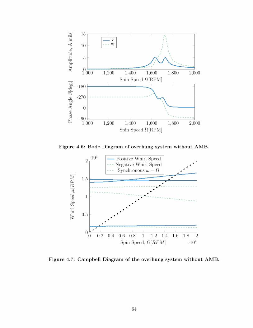
1,000 1,200 1,400 1,600 1,800 2,0000
5
10
15
Spin Speed Ω[RPM]
Am
plitu
de,
A[m
ils]
vw
1,000 1,200 1,400 1,600 1,800 2,000-90
0
-270
-180
Spin Speed Ω[RPM]
Phas
eA
ngl
eβ
[deg
.]
Figure 4.6: Bode Diagram of overhung system without AMB.
0 0.2 0.4 0.6 0.8 1 1.2 1.4 1.6 1.8 2
·104
0
0.5
1
1.5
2·104
Spin Speed, Ω[RPM ]
Whir
lSp
eed,ω
[RPM
]
Positive Whirl SpeedNegative Whirl SpeedSynchronous ω = Ω
Figure 4.7: Campbell Diagram of the overhung system without AMB.
64

−500 −400 −300 −200 −100 0
500
1,000
1,500
<(s)
=(s)
Positive Whirl SpeedNegative Whirl Speed
Figure 4.8: Roots Locus of overhung system without AMB.
4.3.1 Active Magnetic Bearing
Magnetic pole-rotor relationship will be derived based on the detailed derivation in
[5], with influence from [3]. Assumptions made in this model are as follows:
• Air gap between the magnet pole face and the rotor is vanishingly small com-
pared to the diameter of the shaft.
• Flux leakage from the magnetic pole is negligible.
• Curvature of rotor surface under the pole face is ignored.
• A linear relationship of flux density and magnetic field is assumed.
• Hysteresis of the magnetic field is negligible.
These assumptions lead to a magnetic force due to coil current in the relationship of
Fm =−kmi2
l2g(4.1)
65

<(s): -2.6,
=(s): 1633[RPM]
Ω: 1633[RPM]
(a) Mode Shape 1.
<(s): -1.5e+02,
=(s): 1.015e+04[RPM]
Ω: 1.015e+04[RPM]
(b) Mode Shape 2.
<(s):-3.7e+02,
=(s): 1.451e+04[RPM]
Ω: 1.451e+04[RPM]
Beam ShapeOrbit Path
(c) Mode Shape 3.
where, km = µ0ApN2
4, and µ0 = 4π× 10−7 is the absolute permeability in free air, N is
the number of coil turns, Ap is the pole face area, i is the supplied electrical current,
and lg is the air gap.
Consider a set of magnetic pole pairs in each the y & z directions (i.e. One on
the left and one on the right; one on top and one on bottom), where each pole pair
has its own electrical circuit. There are four total magnets in this model, two in each
direction, and eight total poles where two form a magnet. All poles in the neutral
position of the system will have a nominal air gap of g0 and will be supplied by a
bias current of i0. Deviations of the current from this bias will be considered as iy
and iz. Deviations of the position from this neutral position are the displacements
of the rotor at this beam axis location, v, & w. Therefore, total current will be
(i0± iy) & (i0± iz) for opposing poles in the y & z directions respectively. Similarly,
total gaps are given by (g0 ± v) & (g0 ± w). Using these new definitions for the gap
and current, and summing forces in the y & z directions leads to the total forces
Fy = Km
(i0 + iyg0 + v
)2
−(i0 − iyg0 − v
)2
& Fz = Km
(i0 + izg0 + w
)2
−(i0 − izg0 − w
)2
(4.2)
66

where, Km = km cos(α), and α is half of the angle between the poles of a magnet.
Linearizing the magnetic force equations (4.2), while assuming the operating point
for the system is where all positions and control currents are zero, results in
Fy = kiiy + kyv, & Fz = kiiz + kzw (4.3)
where, ki = 4Kmi0g20
is the current stiffness developed by the bias current, and ky =
kz = ks = −4Kmi20g30
.
4.3.1.1 Proportional Derivative Control
A control algorithm is used to control the current sent to each pair of poles based on
the position (proportional) and velocity (derivative) of the rotor. It is assumed that
each set of pole pairs will receive opposite currents to act as a unit. Current control
is given by
iy = −kg(kpv + kvv), & iz = −kg(kpw + kvw) (4.4)
where, kg is the power amplifier gain, kp is the proportional gain, and kv is the
derivative gain. The total linearized force becomes
Fy = −(kgkikp − ks)v − kgkikvv, & Fz = −(kgkikp − ks)w − kgkikvw (4.5)
so then the stiffness of the AMB is kmag = (kgkikp − ks) and the damping is dmag =
kgkikv. As an equation of nodal stiffness and damping in the finite element system it
can be represented by
Dm~qk + Km~qk = 0 (4.6)
67

where,
Km =
kmag 0 0 0 0 0
0 kmag 0 0 0 0
0 0 0 0 0 0
0 0 0 0 0 0
0 0 0 0 0 0
0 0 0 0 0 0
Dm =
dmag 0 0 0 0 0
0 dmag 0 0 0 0
0 0 0 0 0 0
0 0 0 0 0 0
0 0 0 0 0 0
0 0 0 0 0 0
4.4 Addition of Magnetic Bearing to the Rotor Model
In order to measure the effectiveness of the AMB, the Stability of the theoretical
model before the addition is shown in Figure 4.10a. The magnetic bearing added is
modeled after a magnetic bearing that is currently in the lab at California Polytechnic
State University. This theoretical exercise is intended to be followed by experimental
verification not included in this work. The parameters used are listed in 4.3 as well
as the control values whose determinations will be evaluated.
First the axial position of the AMB must be determined. By inspection of the
mode shapes, it is evident that in the first mode (the mode we are most concerned
about suppressing) a shape exists with increasing amplitude toward the end of the
beam after the second bearing. It is also known that the source of vibration, the
rotating disk, is located at nodal index six. With both these pieces of information,
node seven is chosen as a starting point for the AMB for two reasons: having the
AMB closer to the source of vibration reduces the phase lag between the source and
the bearing, increasing the effectiveness of control; amplitude of vibration, according
to the mode shape, is higher on the outboard side of the disk and placing the AMB on
this side will minimize more vibration. Additionally, this location should significantly
suppress the second mode of vibration as node seven is near the maximum amplitude
of that mode as well.
68

In order to choose a value for bias current, ib, and provide upper range estimates
of the controller outputs, kv, & kp, the maximum expected current output of the
control loop must be determined. ib will be set so that under peak power output,
in the expected speed range, the control current will push the total current output
beyond the system limits.
Knowing that the amplitude of vibration, A, in the experimental system peaks
at about 10 mils, or 2.54 × 10⁻⁴[m], the greatest possible velocity for synchronous
vibration is determined using the simple equation vel = (A/2)ω, where ω is the whirl
speed in rad/s. Under the assumption of synchronous vibration, ω during the natural
frequency is then 167.6[Rad/s]. Leading to a velocity, vel, of 0.02[m/s]. Also, another
possible peak velocity occurs in the upper speed range. Knowing that the amplitude of
vibration after the first natural frequency is equal to the eccentricity of the unbalance,
with an eccentricity of 1× 10⁻⁵, and an upper speed of 15000[RPM ], the velocity is
calulated to be 0.008[m/s]. Since the estimated velocity during the natural frequency
is higher, it will be used to limit the output of the AMB controller. Total voltage
supply of most digital to analog converters is limited to 10[V ]. So the control voltage
is calculated to be within this range for the given velocity and positions that will be
seen under synchronous vibration. This results in a limitation of the term kv, which
is proportional to the voltage control signal that is sent to the amplifier for conversion
to control current. A value of 480[V s/m] would max the converter, so the value to
be determined must be less than this. With a similar, but separate, evaluation of the
displacement leads to a maximum allowable value of 500000[V/m] for kp–a value not
anticipated to be necessary. The maximum force due to unbalance is εmdΩ2, where ε
is the eccentricity, and md is the mass of the disk. At the maximum speed expected
of 15000[RPM ], the force will be 24[N ]. To counteract this force with a single coil
would require 1.25[A], or 0.625[A] per coil in a opposing pair. The amplifier gain
is assumed to be programmable to kg = 1[A/V ], this leads to a reasonable choice
69

of bias current at 0.5[A] to maintain a good resolution on the voltage output of the
controller. Under the operating conditions described, the control voltage should not
exceed 1.25[V ], and will rest at an output of 0.5[V ]. Now in the next section, control
parameters kv & kp will be determined to maximize stability of the system while also
minimizing vibration.
To determine best derivative control constant (kv), the proportional control con-
stant (kp) was set to zero. kv is increased until the first mode on the Roots locus(fig.
4.8) moves away from the imaginary axis, becoming more damped. The resulting
movement of the Roots on the Roots Locus is given in Figure 4.11. Note that be-
cause of bias current flowing through the bearing, a baseline stiffness of kS is present
in the system even withou kp. None of the modes that appear on the roots locus
of the system with kp = 0, & kv = 10[V ms
] control algorithm cross the real plane–
this demonstrates the stability of the new system. Stability of the system with the
AMB addition is confirmed in the stability plot of Figure 4.10b. In fact from the
roots locus with kv = 1 to the roots locus with kv = 10 the first mode of vibration
is completely relegated to the imaginary axis and not reaching break-away for this
entire speed range–this indicates that the first mode has been over-damped. With
additional damping through the increase of kv it would be possible to over-damp
the second mode as well, but in the speed range given, it would not improve the
performance.
Proportional control, kp, was added after the ideal derivative control was deter-
mined, but it did not improve the performance of the controller. It is the case that
the stiffness of the bearing inherent to the bias current is sufficient. In any case,
proportional control in this scenario is only adding stiffness to the system, and with
the objective being to minimize vibration, kp is not effective. So the optimal control
is determined to be with kp = 0, & kv = 10[V s/m]. The remaining parameters for
this resulting controller are listed in table 4.3. It is worthwhile to note that this
70

Table 4.3: Active Magnetic Bearing Parameters.
α[rad] g0[m] i0[A] kp[Vm
] kv[V sm
] kg[AV
] N [#] Ap[m2]
π8
2.5× 10⁻³ 0.5 0 10 1 800 5100∗100
optimal control is standing on the basis that the feedback is of synchronous vibration
only. In a scenario where there is significant sub or super-synchronous vibrations,
this controller may exceed its voltage limit. It is recommended that the feedback
signal be filtered to match rotor speed to ensure this scenario does not take place.
Furthermore, without at least low-pass filtering of the feedback signal the control
would certainly provide out of range signals due to the volatile nature of derivatives
of discrete signals.
The frequency spectrum is provided showing the result of the AMB application
in the bode diagram of Figure 4.12. Certainly it can be concluded that the AMB is
successfully performing the desired task of reducing the vibration while also inproving
the stability of the system.
The result from this synthesis exercise can be implemented on the actual exper-
imental test rig with the AMB set to the control parameters suggested. The power
of the finite element method in this application is the ability to move components
around with ease. For instance, with the changing of just two parmeters in the input
file for this model, a new simulation is created for complete levitation of the overhung
rotor. The AMB is put in place of bearing b and the resulting frequency spectrum is
plotted in Figure 4.13
71

0.5 1 1.5 2·104
0
5
4646
[RP
M]
Speed, Ω[RPM ]Max
imum<
(s)
(a) Stability plot of rotor without AMB,
threshold of stability: 4646[RPM ].
0.5 1 1.5 2·104
−300
−200
−100
0
Speed, Ω[RPM ]
Max
imum<
(s)
(b) Stability plot of rotor with AMB, indicates
complete stability through speed range.
−600 −500 −400 −300 −200 −100 0
200
400
600
800
1,000
1,200
1,400
1,600
1,800
<(s)
=(s
)
Uncontrolledkp = 0 & kv = 0.0kp = 0 & kv = 0.1kp = 0 & kv = 1.0kp = 0 & kv = 10.
Figure 4.11: Roots locus of Overhung rotor system with varying kv.
72

0 0.2 0.4 0.6 0.8 1 1.2 1.4 1.6 1.8 2
·104
-270
-180
-90
0
Spin Speed Ω[RPM]
Phas
eA
ngl
e,β
[deg
] vw
v, with AMBw, with AMB
0 0.2 0.4 0.6 0.8 1 1.2 1.4 1.6 1.8 2
·104
10−2
100
102
Spin Speed Ω[RPM]
Am
plitu
de,
A[m
ils]
Figure 4.12: Bode diagram at node 6 comparing the rotor withoutAMB(solid) and with AMB(dashed).
0 0.2 0.4 0.6 0.8 1 1.2 1.4 1.6 1.8 2
·104
-270
-180
-90
0
Spin Speed Ω[RPM]
Phas
eA
ngl
e,β
[deg
] vw
v, with AMBw, with AMB
0 0.2 0.4 0.6 0.8 1 1.2 1.4 1.6 1.8 2
·104
10−2
100
102
Spin Speed Ω[RPM]
Am
plitu
de,
A[m
ils]
Figure 4.13: Bode diagram at node 6 comparing the rotor withoutAMB(solid) and with AMB(dashed) for complete levitation at node 4.
73

Chapter 5
CONCLUSION
5.1 Summary
The aim of this work was to provide a basis for development of rotordynamic mod-
els, and their comparison to experimental results. A finite element method designed
specifically for creation of these models was presented. Techniques for analyzing mod-
els in the frequency domain were explained and the results demonstrated. Methods for
also analyzing experimental vibration signals provided a correlation between models
and experimental results. Correlations between experimental results and theoretical
models were explored in the optimization of an overhung rotor levitated by an active
magnetic bearing. Interpretations of both model and experimental signal analysis
were provided to lend in understanding results. Resulting analyses and interpreta-
tions can be used to identify problems with existing rotating machines as well as aid
in the design process of new rotating machines.
5.2 Future Work
This work is intended to be a building block on which future students at Cal Poly
may build more advanced models and signal processing techniques in the field of
rotordynamics. Possible future projects related to the extension of this work are:
• an experiment with the application of an active magnetic bearing on an over-
hung rotor system, using the parameters and methods determined in this work
• extension of this finite element model to include non-linear internal damping
constitutive relationships
74

• extension of this finite element model to include a more detailed disk model for
the analysis of turbomachines
• extension of this finite element model to include damping effects from various
fittings and couplings
75
BIBLIOGRAPHY
[1] L. Andersen and S. R. Nielsen. Elastic beams in three dimensions. Aalborg
University, 2008.
[2] D. E. Bently and C. T. Hatch. Fundamentals of rotating machinery
diagnostics. Mechanical Engineering-CIME, 125(12):53–54, 2003.
[3] D. W. Childs. Turbomachinery rotordynamics: phenomena, modeling, and
analysis. John Wiley & Sons, 1993.
[4] R. R. Craig and A. J. Kurdila. Fundamentals of structural dynamics. John
Wiley & Sons, 2006.
[5] A. Das, M. Nighil, J. Dutt, and H. Irretier. Vibration control and stability
analysis of rotor-shaft system with electromagnetic exciters. Mechanism and
Machine Theory, 43(10):1295–1316, 2008.
[6] B. Ertas and J. Vance. The influence of same-sign cross-coupled stiffness on
rotordynamics. Journal of Vibration and Acoustics, 129(1):24–31, 2007.
[7] L. Forrai. Stability analysis of symmetrical rotor-bearing systems with internal
damping using finite element method. In International Gas Turbine and AeroB
engine Congress and Exhibition, Birmingham, UK, 1996.
[8] G. Genta. Consistent matrices in rotor dynamic. Meccanica, 20(3):235–248,
1985.
[9] G. Genta. On a persistent misunderstanding of the role of hysteretic damping
in rotordynamics. TRANSACTIONS-AMERICAN SOCIETY OF
MECHANICAL ENGINEERS JOURNAL OF VIBRATION AND
ACOUSTICS, 126(3):459–461, 2004.
76

[10] G. Genta. Dynamics of rotating systems. Springer Science & Business Media,
2007.
[11] T. Gmur and J. Rodrigues. Shaft finite elements for rotor dynamics analysis.
Journal of Vibration and Acoustics, 113(4):482–493, 1991.
[12] U. Goerguelue. Beam theories the difference between euler-bernoulli and
timoschenko. Lecture Handouts, 2009.
[13] P. Goldman and A. Muszynska. Application of full spectrum to rotating
machinery diagnostics. Orbit, 20(1):17–21, 1999.
[14] L. Greenhill, W. Bickford, and H. Nelson. A conical beam finite element for
rotor dynamics analysis. Journal of Vibration, Acoustics, Stress, and Reliability
in Design, 107(4):421–430, 1985.
[15] M. A. Kandil. On rotor internal damping instability. PhD thesis, Imperial
College London (University of London), 2005.
[16] B. Kirchgaßner. Finite elements in rotordynamics. Procedia Engineering,
144:736–750, 2016.
[17] Y. Luo. An efficient 3d timoshenko beam element with consistent shape
functions. Adv. Theor. Appl. Mech, 1(3):95–106, 2008.
[18] A. Muszynska. Rotordynamics. CRC press, 2005.
[19] H. Nelson. A finite rotating shaft element using timoshenko beam theory.
Journal of mechanical design, 102(4):793–803, 1980.
[20] H. Nelson and J. McVaugh. The dynamics of rotor-bearing systems using finite
elements. Journal of Engineering for Industry, 98(2):593–600, 1976.
77

[21] H. N. Ozguven and Z. L. Ozkan. Whirl speeds and unbalance response of
multibearing rotors using finite elements. Journal of vibration, acoustics, stress,
and reliability in design, 106(1):72–79, 1984.
[22] E. Swanson, C. D. Powell, and S. Weissman. A practical review of rotating
machinery critical speeds and modes. Sound and vibration, 39(5):16–17, 2005.
[23] H. Wettergren and K.-O. Olsson. Dynamic instability of a rotating asymmetric
shaft with internal viscous damping supported in anisotropic bearings. Journal
of sound and vibration, 195(1):75–84, 1996.
[24] E. Zorzi and H. Nelson. Finite element simulation of rotor-bearing systems
with internal damping. Journal of Engineering for Power, 99(1):71–76, 1977.
78

APPENDICES
Appendix A
BERNOULLI-EULER BEAM EQUATION
Assumptions used to derive the Bernoulli-Euler beam equation are (Complete deriva-
tion in [4]):
1. Beam is bending in a plane, in this case in the y-direction, where the x-direction
is along the length of the beam.
2. The neutral axis undergoes no deformation in the longitudinal direction.
3. Cross sections remain plane and perpendicular to the nuetral axis.
4. The material is linear-elastic.
5. Stresses in the y and z direction are negligible compared to those in the x
direction.
6. Rotary inertial effects are not considered.
7. Mass density is constant at each cross section, so that each mass center is
coincident with the centroid of that section.
Using kinematics and assumptions 2 & 3, the strain in the x direction may be related
to the curvature of the beam, µ(x, t), and the distance from the neutral axis by
ε = −yµ
(A.1)
then, with assumption 4 & 7 the relation from curvature to moment is
M(x, t) =EI
µ(A.2)
79

x
y
F (x, t)
F (x+ ∆x, t)
M(x+ ∆x, t)M(x, t)
v(x, t)
G
Figure A.1: Free body diagram of a beam section in planar bending.
where E, Young’s modulus, and I, area moment of inertia are constant in cross
sections. By using Newton’s laws and the free body diagram of a single beam element,
see Figure A.1, the equations of motion are summarized as:
∑Fy = ∆mv &
∑MG = 0 (A.3)
Moment equation is represented as moments summarized at the center of mass, G.
The right hand side of moment equation of EOM (A.3) is know to be null due to
assumption 6. Applying Newton’s equations (A.3) to the FBD of Figure A.1 results
in the force equation
F (x, t)− F (x+ ∆x, t) = ρA∆x∂2v
∂t2(A.4)
and moment equation
−M(x, t) +M(x+ ∆x, t) + F (x, t)
(−∆x
2
)+ [−F (x+ ∆x, t)]
(∆x
2
)= 0 (A.5)
Taking the limit of equations (A.4) & (A.5) as ∆x→ 0 results in equations (A.6) &
(A.7) respectively.
∂F
∂x= −ρA∂
2v
∂t2(A.6)
∂M
∂x− F = 0 (A.7)
80

Assuming the beam slope, ∂v∂x
, remains relatively small, then linearized curvature of
the beam is inversely related to ∂2v∂x2
. Substituting this linearized curvature in (A.2)
produces
M(x, t) = EI∂2v
∂x2(A.8)
Using linearized moment equation (A.8), combined with (A.6) & (A.7) lends the Euler
beam equation
∂2
∂x2
(EI
∂2v
∂x2
)= −ρA∂
2v
∂t2(A.9)
This is the governing differential equation for transverse motion of a slender beam.
This equation is not suitable for an application involving lengths that are not much
greater than the width of the beam [10].
81

Appendix B
ROTORFEM MATLAB CODE FOR CONSTRUCTING AND ANALYZING FEM
MODELS
B.1 Main Object File
1 c l a s s d e f RotorFEM< handle
2 %MODEL Summary o f t h i s c l a s s goes here
3 % Deta i l ed exp lanat ion goes here
4
5 p r op e r t i e s
6 M
7 C
8 K
9 F
10 i n p u t f i l e
11 npos
12
13 end
14 p r op e r t i e s ( Access = pr i va t e )
15
16 end
17 methods
18 func t i on obj = Model ( i nput f i l ename )
19 i f narg in == 1
20 obj . Assem( input f i l ename ) ;
21 obj . i n p u t f i l e = input f i l ename ;
22 end
23 end
24 end
25
26 end
B.2 Matrix Assembly File
1 func t i on Assem( obj , i n p u t f i l e )
2 run ( i n p u t f i l e )
3
4 nodes = s i z e ( elems , 1 ) +1;
5 npos = ze ro s ( nodes , 1 ) ;
6 f o r i i = 1 : nodes−1
7 npos ( i i +1) = npos ( i i ) + elems ( i i , 2 ) ;
8 end
9 obj . npos = npos ;
10
11 K = ze ro s ( nodes *DOF, nodes *DOF) ;
82

12 C = ze ro s ( nodes *DOF, nodes *DOF) ;
13 M = zero s ( nodes *DOF, nodes *DOF) ;
14 F = ze ro s ( nodes *DOF, 1 ) ;
15 f o r i i = 1 : 1 : s i z e ( elems , 1 )
16 E = mate ( elems ( i i , 1 ) ,2 ) ;
17 l = elems ( i i , 2 ) ;
18 do = elems ( i i , 3 ) ;
19 i f s i z e ( elems ( i i , : ) )<4
20 di =0;
21 e l s e
22 do=elems ( i i , 4 ) ;
23 end
24 I = obj . AInert (do , d i ) ;
25 A = obj . Area (do , d i ) ;
26 rho = mate ( elems ( i i , 1 ) ,3 ) ;
27 nuv = mate ( elems ( i i , 1 ) ,4 ) ;
28 poi = mate ( elems ( i i , 1 ) ,5 ) ;
29 Id = obj . Dia Iner t (do , l , rho , d i ) ;
30 Ip = obj . Po l Ine r t (do , l , rho , d i ) ;
31 [ kbe , cbe , mbe ] = obj .TBeam(E, I , l ,A, rho , Id , Ip , nuv , poi ,DOF) ;
32 K = obj .Add(K, kbe , ( i i −1)*DOF+1:( i i +1) *DOF) ;
33 C = obj .Add(C, cbe , ( i i −1)*DOF+1:( i i +1) *DOF) ;
34 M = obj .Add(M,mbe , ( i i −1)*DOF+1:( i i +1) *DOF) ;
35 end
36
37 i f e x i s t ( ' d i sk s ' , 'var ' )
38 f o r i i = 1 : 1 : s i z e ( d i sks , 1 )
39 do = d i sk s ( i i , 3 ) ;
40 l = d i sk s ( i i , 2 ) ;
41 rho = mate ( d i s k s ( i i , 1 ) ,3 ) ;
42 a = d i sk s ( i i , 4 ) ;
43 Ki = d i sk s ( i i , 5 ) ;
44 i f s i z e ( d i s k s ( i i , : ) )<7
45 di =0;
46 e l s e
47 di=d i sk s ( i i , 7 ) ;
48 end
49 md = obj . Mass (do , l , rho , d i ) ;
50 Ip = obj . Po l Ine r t (do , l , rho , d i ) ;
51 Id = obj . Dia Iner t (do , l , rho , d i ) ;
52 [ mi , gi , f i ] = obj . Disk (md, Id , Ip , a , Ki ,DOF) ;
53 M = obj .Add(M,mi , ( d i s k s ( i i , 6 ) *DOF−DOF+1: d i s k s ( i i , 6 ) *DOF) ) ;
54 C = obj .Add(C, gi , ( d i s k s ( i i , 6 ) *DOF−DOF+1: d i s k s ( i i , 6 ) *DOF) ) ;
55 F = obj . AddVect (F , f i , ( d i s k s ( i i , 6 ) *DOF−DOF+1: d i s k s ( i i , 6 ) *DOF) ) ;
56 end
57 end
58
59 f o r i i = 1 : 1 : s i z e ( bears , 1 )
60 kx = beartypes ( bears ( i i , 1 ) ,2 ) ;
61 ky = beartypes ( bears ( i i , 1 ) ,3 ) ;
62 c = beartypes ( bears ( i i , 1 ) ,4 ) ;
63 [ ki , c i ] = obj . Bear (kx , ky , c ,DOF) ;
64 K = obj .Add(K, ki , ( bears ( i i , 2 ) *DOF−DOF+1: bears ( i i , 2 ) *DOF) ) ;
65 C = obj .Add(C, c i , ( bears ( i i , 2 ) *DOF−DOF+1: bears ( i i , 2 ) *DOF) ) ;
66
83

67 end
68 i f e x i s t ( 'mags ' , 'var ' )
69 f o r i i = 1 : 1 : s i z e (mags , 1 )
70 o l dd i r = pwd ;
71 cd ( char ( mag f i l e (mags ( i i , 1 ) ,2 ) ) )
72 Magfn = s t r2 func ( char ( mag f i l e (mags ( i i , 1 ) ,3 ) ) ) ;
73 [ ki , c i ] = Magfn ( ) ;
74 cd ( o l dd i r )
75 K = obj .Add(K, ki , ( mags ( i i , 2 ) *DOF−DOF+1:mags ( i i , 2 ) *DOF) ) ;
76 C = obj .Add(C, c i , ( mags ( i i , 2 ) *DOF−DOF+1:mags ( i i , 2 ) *DOF) ) ;
77
78 end
79 end
80 obj .M = M;
81 obj .C = C;
82 obj .K = K;
83 obj .F = F;
B.3 Elemental Matrices
1 func t i on [ K,D,M ] = TBeam( obj , E, I , l ,A, rho , Id , Ip , nuv , poi ,DOF )
2 %TBeam Timoshenko beam element
3 % disp1y di sp1z ang1y ang1z disp2y d i sp2z ang2y ang2z disp1x ang1x disp2x ang2x
4 %
5 %| | disp1y
6 %| | disp1z
7 %| | ang1y
8 %| | ang1z
9 %| | disp2y
10 %| | disp2z
11 %| | ang2y
12 %| | ang2z
13 %| | ang2x
14 %% Prope r t i e s %%
15 k = 6*(1+ poi ) /(7+6* poi ) ;
16 G = E/2/(1+ poi ) ;
17 alph = 12*E* I /k/G/A/ l ˆ2 ;
18 %% Var iab l e s %%
19 syms x
20 z = x/ l ;
21 %% Shape Functions %%
22 N1 = 1−z ;
23 N2 = z ;
24 Tt1 = (1/(1+ alph ) ) * (2 * z ˆ3 − 3* z ˆ2 − alph * z + 1 + alph ) ;
25 Tt2 = (1/(1+ alph ) ) *(−2* zˆ3+3*zˆ2+alph * z ) ;
26 Tr1 = ( l /(1+alph ) ) * ( z ˆ3 − (2+1/2* alph ) * z ˆ2 + (1+1/2* alph ) * z ) ;
27 Tr2 = ( l /(1+alph ) ) * ( z ˆ3 − (1−1/2* alph ) * z ˆ2 − 1/2* alph * z ) ;
28 Rt1 = 6/ l *(1/(1+ alph ) ) * ( zˆ2−z ) ;
29 Rt2 = −Rt1 ;
30 Rr1 = (1/(1+ alph ) ) * (3 * z ˆ2 − (4+alph ) * z + 1 + alph ) ;
31 Rr2 = (1/(1+ alph ) ) * (3 * z ˆ2 − (2−alph ) * z ) ;
32 %% Transformation Mat r i c i e s %%
84

33 P = [0 0 0 0 0 0 ;
34 0 0 0 0 0 0 ;
35 0 −1 0 0 0 0 ;
36 1 0 0 0 0 0 ;
37 0 0 0 0 0 0 ;
38 0 0 0 0 0 0 ] ;
39 Di = [12 *E* I / alph / l ˆ2 0 0 0 0 0 ;
40 0 12*E* I / alph / l ˆ2 0 0 0 0 ;
41 0 0 E* I 0 0 0 ;
42 0 0 0 E* I 0 0 ;
43 0 0 0 0 E*A 0 ;
44 0 0 0 0 0 12*E* I / alph / l ˆ2/A*2* I ] ;
45 Mi = diag ( [ rho *A* l , rho *A* l , Id , Id , rho *A* l , Ip ] ) . / l ;
46 Gi = kron ( diag ( [ 0 , 1 , 0 ] ) , [ 0 , Ip ;−Ip , 0 ] ) . / l ;
47 T = kron ( diag ( [ 1 , 1 , 0 ] ) , [ 0 , 1 ; −1 , 0 ] ) ;
48 N = [ Tt1 0 0 Tr1 Tt2 0 0 Tr2 0 0 0 0 ;
49 0 Tt1 Tr1 0 0 Tt2 Tr2 0 0 0 0 0 ;
50 0 Rt1 Rr1 0 0 Rt2 Rr2 0 0 0 0 0 ;
51 Rt1 0 0 Rr1 Rt2 0 0 Rr2 0 0 0 0 ;
52 0 0 0 0 0 0 0 0 N1 0 N2 0 ;
53 0 0 0 0 0 0 0 0 0 N1 0 N2 ] ;
54 %% DOF Mod i f i c a t i on s%%
55 switch DOF
56 case 6
57 I = diag ( [ 1 , 1 , −1 ,1 , 1 , 1 ] ) ;
58 N = I *N* [ I , z e r o s (6 ) ; z e ro s (6 ) , I ] ; % Adjust f o r use o f −angy ,−ang1 , 2 y d e f i n i t i o n s in shape
func t i on s
59 case 4
60 P = P( 1 : 4 , 1 : 4 ) ;
61 Di = Di ( 1 : 4 , 1 : 4 ) ;
62 Mi = Mi ( 1 : 4 , 1 : 4 ) ;
63 Gi = Gi ( 1 : 4 , 1 : 4 ) ;
64 T = T( 1 : 4 , 1 : 4 ) ;
65 I = diag ( [1 ,1 , −1 ,1 ] ) ; % Adjust f o r use o f −angy ,−ang1 , 2 y d e f i n i t i o n s in shape func t i on s
66 N = I *N(1 : 4 , 1 : 8 ) * [ I , z e r o s (4 ) ; z e ro s (4 ) , I ] ;
67 case 2
68 P = P( 2 : 3 , 2 : 3 ) ;
69 Di = Di ( 2 : 3 , 2 : 3 ) ;
70 Mi = Mi ( 2 : 3 , 2 : 3 ) ;
71 Gi = Gi ( 2 : 3 , 2 : 3 ) ;
72 T = T( 2 : 3 , 2 : 3 ) ;
73 N = N( 2 : 3 , [ 2 , 3 , 6 , 7 ] ) ;
74 end
75 %% Elemental I n t e g r a t i on %%
76 B = d i f f (N. ' , x ) − N. ' *P;
77 B = B. ' ;
78 K B = in t (B. ' *Di *B, x , 0 , l ) ;
79 K C = in t (B. ' *T*Di *B, x , 0 , l ) ;
80 G = in t (N. ' *Gi *N, x , 0 , l ) ;
81 M = in t (N. ' *Mi*N, x , 0 , l ) ;
82 %% Case o f symbol ic I n t e g r a t i on %%
83 i f i s a ( l , 'sym ' ) | | i s a (E, 'sym ' ) | | i s a ( I , 'sym ' ) | | i s a (nuv , 'sym ' )
84 e l s e
85 K B = double (K B) ;
86 K C = double (K C) ;
85
87 G = double (G) ;
88 M = double (M) ;
89 end
90 K = K B + nuv . *1 i . *K C;
91 D = nuv . *K B + 1 i . *G;
92
93 end
1 func t i on [Md,Gd,Fd ] = Disk ( obj ,md, Id , Ip , a , Ki ,DOF)
2 %% Creates Disk nodal s t i f f n e s s matrix in the form :
3 % disp1x disp1y ang1x ang1y
4 %
5 %| | disp1x
6 %| | disp1y
7 %| | ang1x
8 %| | ang1y
9
10 %% Begin Function
11 Fx = md*a ;
12 Fy = md*a ;
13 Mx = ( Id−Ip ) *Ki ;
14 My = ( Id−Ip ) *Ki ;
15 Gi=[0 , Ip ;−Ip , 0 ] ;
16 switch DOF
17 case 6
18 Md = diag ( [md,md, Id , Id ,md, Ip ] ) ;
19 Gd = 1 i * kron ( diag ( [ 0 , 1 , 0 ] ) ,Gi ) ;
20 Fd = [Fx ; Fy ; Mx; My; 0 ; 0 ] ;
21 case 4
22 Md = diag ( [md,md, Id , Id ] ) ;
23 Gd = 1 i * kron ( diag ( [ 0 , 1 ] ) ,Gi ) ;
24 Fd = [Fx ; Fy ; Mx; My ] ;
25 case 2
26 Md = diag ( [md, Id ] ) ;
27 Gd = 1 i * [ 0 , 0 ; 0 , Ip ] ;
28 Fd = [Fx ; My ] ;
29 end
30 % Fx = md*a * (wˆ2* cos ( theta+phi1 )−alph * s i n ( theta+phi1 ) ) ; %N, Forcing funt ion at d i sk 1
31 % Fy = md*a * (wˆ2* s i n ( theta+phi1 )+alph * cos ( theta+phi1 ) ) ; %N, Forcing funt i on at d i sk 2
32 % Mx = −wˆ2*( Ip − Id ) *Ki * cos ( theta+phi2 ) ; %N, Forcing funt ion at d i sk 1
33 % My = wˆ2*( Ip − Id ) *Ki * s i n ( theta+phi2 ) ; %N, Forcing funt i on at d i sk 2 ;
34 end
1 func t i on [ Kb,Cb ] = Bear ( obj , kx , ky , c ,DOF)
2 %% Creates bear ing nodal s t i f f n e s s matrix in the form :
3 % disp1y di sp1z ang1y ang1z disp1x ang1x
4 %
5 %| | disp1y
6 %| | disp1z
7 %| | ang1y
8 %| | ang1z
9 %| | disp1x
10 %| | ang1x
11 %% Begin func t i on
12 switch DOF
86

13 case 6
14 Kb = diag ( [ kx , ky , 0 , 0 , 0 , 0 ] ) ;
15 Cb = diag ( [ c *kx , c *ky , 0 , 0 , 0 , 0 ] ) ;
16 case 4
17 Kb = diag ( [ kx , ky , 0 , 0 ] ) ;
18 Cb = diag ( [ c *kx , c *ky , 0 , 0 ] ) ;
19 case 2
20 k = mean ( [ kx , ky ] ) ;
21 Kb = diag ( [ k , k ] ) ;
22 Cb = diag ( [ c *k , c *k ] ) ;
23 end
24 end
B.4 Plotting Functions
1 func t i on RootLocus (Model obj ,Omega , plotmodes , ax , l i n e tp , c o l o r )
2 %CAMPBELL Summary o f t h i s func t i on goes here
3 % Deta i l ed exp lanat ion goes here
4 z c i = @(v ) f i nd (v ( : ) . * c i r c s h i f t ( v ( : ) , [−1 0 ] ) <= 0) ;
5 i f narg in < 6
6 co l o r = [ 0 , 0 , 0 ] ;
7 i f narg in <5
8 l i n e t p = ' . ' ;
9 end
10 i f narg in < 4
11 f i g u r e
12 ax = axes ;
13 end
14 i f narg in < 3
15 plotmodes = 1 : 2 ;
16 end
17 i f narg in < 2
18 return
19 end
20
21 end
22
23 f o r i i = 1 : 1 : l ength (Omega)
24 w = Omega( i i ) /60*2* pi ;
25 Mnew = Model obj .M;
26 Cnew = r e a l ( Model obj .C) + w. * imag ( Model obj .C) ;
27 Knew = r e a l ( Model obj .K) + w. * imag ( Model obj .K) ;
28 Zer = ze ro s ( s i z e (Mnew) ) ;
29 ey = eye ( s i z e (Mnew) ) ;
30 A = [−Mnewˆ−1*Cnew , −Mnewˆ−1*Knew ;
31 ey , Zer ] ;
32 v1=e i g (A) ;
33 % AA=[Cnew Mnew;Mnew Zer ] ;
34 % B=[Knew Zer ; Zer −Mnew ] ;
35 % v1=e i g (B,−1 i *AA) ;
36 [ ˜ , I ] = ( s o r t ( abs ( ( v1 ) ) ) ) ;
37 e i v ( : , i i ) = v1 ( ( I ) ) ;
87
38 end
39 % whi le min ( abs ( imag ( e i v ( 1 , : ) ) ) ) == 0
40 % e iv ( 1 : 2 , : ) = [ ] ;
41 % end
42 % e iv = e iv ( ˜any ( i snan ( e i v ) | i s i n f ( e i v ) , 2 ) , : ) ;
43
44 hold on
45 f o r j j = 1 : 1 : l ength ( plotmodes )
46
47 % plo t ( ax , r e a l ( e i v ( plotmodes ( j j ) *4−1 , :) ) , ( imag ( e i v ( plotmodes ( j j ) *4−1 , :) ) ) , l i n e tp , ' Color
' , [ 0 . 8 5 0 0 , 0 . 3 2 5 0 , 0 . 0 9 8 0 ] )
48 % p lo t ( ax , r e a l ( e i v ( plotmodes ( j j ) *4−3 , :) ) , ( imag ( e i v ( plotmodes ( j j ) *4−3 , :) ) ) , l i n e tp , ' Color
' , [ 0 , 0 . 4 4 7 0 , 0 . 7 4 1 0 ] )
49 p lo t3 ( r e a l ( e i v ( plotmodes ( j j ) *4−1 , :) ) , abs ( imag ( e i v ( plotmodes ( j j ) * 4 , : ) ) ) ,Omega , l i n e tp , 'Color ' ,
co lo r , 'MarkerSize ' , 1 ) ;%, 'o ' , 'Color ' , [ 0 . 8 5 00 , 0 . 3 2 50 , 0 . 0 9 80 ] , ' MarkerSize ' , 3 )
50 p lo t3 ( r e a l ( e i v ( plotmodes ( j j ) *4−3 , :) ) , abs ( imag ( e i v ( plotmodes ( j j ) *4−2 , :) ) ) ,Omega , l i n e tp , 'Color ' ,
co lo r , 'MarkerSize ' , 1 ) ;% , ' . ' , ' Color ' , [ 0 , 0 . 4 4 7 0 , 0 . 7 4 10 ] , ' MarkerSize ' , 4 )
51 % plot3 ( r e a l ( e i v ( plotmodes ( j j ) *4−0 , :) ) , imag ( e i v ( plotmodes ( j j ) *4−0 , :) ) ,Omega , ' . ' , ' Color
' , [ 0 , 0 . 4 4 7 0 , 0 . 7 4 1 0 ] )
52 % plot3 ( r e a l ( e i v ( plotmodes ( j j ) *4−2 , :) ) , imag ( e i v ( plotmodes ( j j ) *4−2 , :) ) ,Omega , ' . ' , ' Color
' , [ 0 , 0 . 4 4 7 0 , 0 . 7 4 1 0 ] )
53 % r ( 1 , : ) = r e a l ( e i v ( plotmodes ( j j ) *4−1 , :) ) ;
54 % r ( 2 , : ) = r e a l ( e i v ( plotmodes ( j j ) *4−3 , :) ) ;
55 % ZeroCross1 = z c i ( r ( 1 , : ) ) ;
56 % ZeroCross2 = z c i ( r ( 2 , : ) ) ;
57 % i f isempty ( ZeroCross1 )
58 % e l s e
59 % s t r c r o s s 1 = [ num2str (Omega( ZeroCross1 (1) ) ,4 ) ' (RPM) ' newl ine ] ;
60 % text ( ax , 0 , abs ( imag ( e i v ( plotmodes ( j j ) *4−1 , ZeroCross1 (1) ) ) ) , s t r c r o s s 1 , ' HorizontalAlignment ' , '
r ight ' , ' Vert ica lAl ignment ' , ' bottom ' , 'FontWeight ' , ' bold ' ) ;
61 % p lo t ( ax , 0 , abs ( imag ( e i v ( plotmodes ( j j ) *4−1 , ZeroCross1 (1) ) ) ) , '*k ' ) ;
62 % end
63 % i f isempty ( ZeroCross2 )
64 % e l s e
65 % s t r c r o s s 2 = [ num2str (Omega( ZeroCross2 (1) ) ,4 ) ' (RPM) ' newl ine ] ;
66 % text ( ax , 0 , abs ( imag ( e i v ( plotmodes ( j j ) *4−3 , ZeroCross2 (1) ) ) ) , s t r c r o s s 2 , ' HorizontalAlignment ' , '
r ight ' , ' Vert ica lAl ignment ' , ' bottom ' , 'FontWeight ' , ' bold ' ) ;
67 % p lo t ( ax , 0 , abs ( imag ( e i v ( plotmodes ( j j ) *4−3 , ZeroCross2 (1) ) ) ) , '*k ' ) ;
68 % end
69 end
70 hold o f f
71 ax . YAxisLocation = ' o r i g i n ' ;
72 ax i s ([− i n f , in f , 0 , i n f ] )
73 x l ab e l ( 'Real ( s ) ' )
74 y l ab e l ( 'Imag ( s ) ' )
75 end
1 func t i on Campbell ( Model obj ,Omega , plotmodes , ax , l i n e t p )
2 %CAMPBELL Summary o f t h i s func t i on goes here
3 % Deta i l ed exp lanat ion goes here
4 i f narg in < 5
5 i f narg in == 2
6 plotmodes = 1 : 2 ;
7 e l s e i f narg in < 2
8 return
88

9 end
10 l i n e t p = ' . ' ;
11 i f narg in < 4
12 ax = [ ] ;
13 end
14 end
15 f o r i i = 1 : 1 : l ength (Omega)
16 w = Omega( i i ) /60*2* pi ;
17 Mnew = Model obj .M;
18 Cnew = r e a l ( Model obj .C) + w. * imag ( Model obj .C) ;
19 Knew = r e a l ( Model obj .K) + w. * imag ( Model obj .K) ;
20 Zer = ze ro s ( s i z e (Mnew) ) ;
21 ey = eye ( s i z e (Mnew) ) ;
22 A = [−Mnewˆ−1*Cnew , −Mnewˆ−1*Knew ;
23 ey , Zer ] ;
24 v1=e i g (A) ;
25 [ ˜ , I ] = so r t ( abs ( ( v1 ) ) ) ;
26 e i v ( : , i i ) = v1 ( I ) ;
27 % e iv ( : , i i )=v1 ;
28 end
29 i f isempty ( ax )
30 f i g u r e
31 ax = axes ;
32 end
33 % whi le min ( abs ( imag ( e i v ( 1 , : ) ) ) ) == 0
34 % e iv ( 1 : 2 , : ) = [ ] ;
35 % end
36 % e iv = e iv ( ˜any ( i snan ( e i v ) | i s i n f ( e i v ) , 2 ) , : ) ;
37
38 hold on
39 f o r j j = 1 : 1 : l ength ( plotmodes )
40 p lo t ( ax ,Omega , abs ( imag ( e i v ( plotmodes ( j j ) *4−2 , :) ) ) /2/ pi *60 , ' . k ' ) ;%, 'Color ' , [ 0 , 0 . 4 4 7 0 , 0 . 7 4 10 ] , '
LineWidth ' , 1 )
41 p lo t ( ax ,Omega , abs ( imag ( e i v ( plotmodes ( j j ) * 4 , : ) ) ) /2/ pi *60 , ' . k ' ) ;%, 'Color
' , [ 0 . 8 5 00 , 0 . 3 2 50 , 0 . 0 9 80 ] , ' LineWidth ' , 1 , ' MarkerSize ' , 4 )
42 % p lo t ( ax ,Omega , ( imag ( e i v ( plotmodes ( j j ) *4−3 , :) ) ) /2/ pi *60 , l i n e tp , ' Color
' , [ 0 , 0 . 4 4 7 0 , 0 . 7 4 10 ] , ' LineWidth ' , 1 )
43 % p lo t ( ax ,Omega , ( imag ( e iv ( plotmodes ( j j ) * 4 , : ) ) ) /2/ pi *60 , l i n e tp , 'Color
' , [ 0 . 8 5 00 , 0 . 3 2 50 , 0 . 0 9 80 ] , ' LineWidth ' , 1 )
44 %
45 % plo t ( ax ,Omega , imag ( e iv ( plotmodes ( j j ) , : ) ) /2/ pi *60 , l i n e tp , ' Color ' , [ 0 , 0 . 4 4 7 0 , 0 . 7 4 10 ] , ' LineWidth
' , 1 )
46
47 end
48 p lo t (Omega ,Omega , '−−k ' , 'LineWidth ' , 2 )
49 % plo t (Omega,−Omega,'−−k ' , 'LineWidth ' , 2 )
50 hold o f f
51 x l ab e l ( 'Spin speed [RPM] ' )
52 y l ab e l ( 'Whirl speed [RPM] ' )
53 t i t l e ( 'Campbell Diagram ' )
54
55
56 end
1 func t i on S t a b i l i t y ( Model obj , Omega , ax , l i n e t p )
89

2 %STABILITY Summary o f t h i s func t i on goes here
3 % Deta i l ed exp lanat ion goes here
4 z c i = @(v ) f i nd (v ( : ) . * c i r c s h i f t ( v ( : ) , [−1 0 ] ) <= 0) ;
5 i f narg in < 4
6 l i n e t p = '−' ;
7 i f narg in < 3
8 f i g u r e
9 ax = axes ;
10 e l s e i f narg in < 2
11 return
12 end
13
14 end
15
16 f o r i i = 1 : 1 : l ength (Omega)
17 w = Omega( i i ) /60*2* pi ;
18 Mnew = Model obj .M;
19 Cnew = r e a l ( Model obj .C) + w. * imag ( Model obj .C) ;
20 Knew = r e a l ( Model obj .K) + w. * imag ( Model obj .K) ;
21
22 Zer = ze ro s ( s i z e (Mnew) ) ;
23 ey = eye ( s i z e (Mnew) ) ;
24 A = [−Mnewˆ−1*Cnew , −Mnewˆ−1*Knew ;
25 ey , Zer ] ;
26 v1=e i g (A) ;
27 e iv ( : , i i ) = so r t ( v1 ) ;
28 end
29 whi le min ( abs ( imag ( e iv ( 1 , : ) ) ) ) == 0
30 e iv ( 1 : 2 , : ) = [ ] ;
31 end
32 e iv = e iv ( ˜any ( i snan ( e i v ) | i s i n f ( e i v ) , 2 ) , : ) ;
33 hold on
34 p lo t (Omega ,max( r e a l ( e i v ) ) , 'LineWidth ' , 1 , ' LineSty l e ' , l i n e t p ) ;
35 ZeroCross = Omega( z c i (max( r e a l ( e i v ) ) ) ) ;
36 i f ˜ isempty ( ZeroCross )
37 s t r c r o s s = [ ' Threshold : ' num2str ( ZeroCross (1 ) ,4 ) 'RPM' ] ;
38 text ( ZeroCross (1 ) ,0 , s t r c r o s s , 'HorizontalAl ignment ' , ' l e f t ' , 'Vert ica lAl ignment ' , 'middle ' , '
FontWeight ' , 'bold ' , 'Rotation ' , 90) ;
39 p lo t ( ZeroCross (1 ) ,0 , ' *k ' ) ; hold o f f
40 end
41 ax . XAxisLocation = ' o r i g i n ' ;
42 x l ab e l ( 'Speed (RPM) ' )
43 y l ab e l ( 'Maximum \Re( s ) ' )
44 t i t l e ( ' S t a b i l i t y r eg i on ' )
45 end
1 func t i on Damping(Model obj ,Omega , plotmodes , ax , l i n e tp , ch )
2 %CAMPBELL Summary o f t h i s func t i on goes here
3 % Deta i l ed exp lanat ion goes here
4 z c i = @(v ) f i nd (v ( : ) . * c i r c s h i f t ( v ( : ) , [−1 0 ] ) <= 0) ;
5
6 i f narg in < 6
7 i f narg in == 2
8 plotmodes = 1 : 2 ;
9 e l s e i f narg in < 2
90

10 return
11 end
12 ch = 'dec ' ;
13 i f narg in < 5
14 l i n e t p = '−' ;
15 end
16 i f narg in < 4
17 f i g u r e
18 ax = axes ;
19 end
20 end
21
22 f o r i i = 1 : 1 : l ength (Omega)
23 w = Omega( i i ) /60*2* pi ;
24 Mnew = Model obj .M;
25 Cnew = r e a l ( Model obj .C) + w. * imag ( Model obj .C) ;
26 Knew = r e a l ( Model obj .K) + w. * imag ( Model obj .K) ;
27
28 Zer = ze ro s ( s i z e (Mnew) ) ;
29 ey = eye ( s i z e (Mnew) ) ;
30 A = [−Mnewˆ−1*Cnew , −Mnewˆ−1*Knew ;
31 ey , Zer ] ;
32 v1=e i g (A) ;
33 [ ˜ , I ] = ( s o r t ( abs ( ( v1 ) ) ) ) ;
34 e i v ( : , i i ) = v1 ( ( I ) ) ;
35 end
36
37 whi le min ( abs ( imag ( e iv ( 1 , : ) ) ) ) == 0
38 e iv ( 1 : 2 , : ) = [ ] ;
39 end
40 e iv = e iv ( ˜any ( i snan ( e i v ) | i s i n f ( e i v ) , 2 ) , : ) ;
41
42 hold on
43 f o r j j = 1 : 1 : l ength ( plotmodes )
44 i d f = plotmodes ( j j ) *4−1; %forward mode index l o c a t i on
45 idb = i d f − 2 ; %backward mode index l o c a t i o n
46 zeta = −r e a l ( e i v ( [ idb , i d f ] , : ) ) . / abs ( e i v ( [ idb , i d f ] , : ) ) ;
47 % de l t a = 2* pi . * zeta . / sq r t (1− zeta . ˆ 2 ) ; %Logarithmic Decriment
48 % de l t a = −2*pi * r e a l ( e i v ( [ idb , i d f ] , : ) ) . / imag ( e i v ( [ idb , i d f ] , : ) ) ;
49 p lo t (Omega , zeta ( 1 , : ) , l i n e tp , 'Color ' , [ 0 , 0 . 4 4 7 0 , 0 . 7 4 1 0 ] , 'LineWidth ' , 1 ) ;
50 p lo t (Omega , zeta ( 2 , : ) , l i n e tp , 'Color ' , [ 0 . 8 5 0 0 , 0 . 3 2 5 0 , 0 . 0 9 8 0 ] , 'LineWidth ' , 1 ) ;
51 ZeroCross1 = Omega( z c i ( zeta ( 1 , : ) ) ) ;
52 ZeroCross2 = Omega( z c i ( zeta ( 2 , : ) ) ) ;
53 i f isempty ( ZeroCross1 )
54 e l s e
55 s t r c r o s s 1 = [ num2str ( ZeroCross1 (1) ,4 ) newl ine ] ;
56 text ( ZeroCross1 (1) ,0 , s t r c r o s s 1 , 'HorizontalAl ignment ' , ' l e f t ' , 'Vert ica lAl ignment ' , 'bottom ' , '
FontWeight ' , 'bold ' ) ;
57 p lo t ( ZeroCross1 (1) ,0 , ' *k ' ) ;
58 end
59 i f isempty ( ZeroCross2 )
60 e l s e
61 s t r c r o s s 2 = [ num2str ( ZeroCross2 (1) ,4 ) newl ine ] ;
62 text ( ZeroCross2 (1) ,0 , s t r c r o s s 2 , 'HorizontalAl ignment ' , ' l e f t ' , 'Vert ica lAl ignment ' , 'bottom ' , '
FontWeight ' , 'bold ' ) ;
91

63 p lo t ( ZeroCross2 (1) ,0 , ' *k ' ) ;
64 end
65
66 end
67 hold o f f
68 ax . XAxisLocation = ' o r i g i n ' ;
69 x l ab e l ( 'Speed (RPM) ' )
70 y l ab e l ( '\ zeta ' )
71 t i t l e ( 'Damping Cha r a c t e r i s t i c s ' )
72
73 end
1 func t i on Shape (Model obj ,Omega , plotmodes , ax , l i n e t p )
2 %CAMPBELL Summary o f t h i s func t i on goes here
3 % Deta i l ed exp lanat ion goes here
4 i f narg in < 5
5 i f narg in < 2
6 return
7 end
8 l i n e t p = '−' ;
9 i f narg in < 4
10 f i g u r e
11 ax = axes ;
12 end
13 end
14
15 syms x ;
16 l =1;
17 z=x/ l ;
18 alph =.25;
19 Tt1 = (1/(1+ alph ) ) * (2 * z ˆ3 − 3* z ˆ2 − alph * z + 1 + alph ) ;
20 Tt2 = (1/(1+ alph ) ) *(−2* zˆ3+3*zˆ2+alph * z ) ;
21 Tr1 = ( l /(1+alph ) ) * ( z ˆ3 − (2+1/2* alph ) * z ˆ2 + (1+1/2* alph ) * z ) ;
22 Tr2 = ( l /(1+alph ) ) * ( z ˆ3 − (1−1/2* alph ) * z ˆ2 − 1/2* alph * z ) ;
23 cp s i = [ Tt1 0 0 Tr1 Tt2 0 0 Tr2 ;
24 0 Tt1 −Tr1 0 0 Tt2 −Tr2 0 ] ;
25 % ps i = [1 − 3* ( x/ l ) ˆ2 + 2* ( x/ l ) ˆ3 , x − 2* l * ( x/ l ) ˆ2 + l * ( x/ l ) ˆ3 , 3* ( x/ l ) ˆ2 − 2* ( x/ l ) ˆ3 , − l * ( x/ l ) ˆ2
+ l * ( x/ l ) ˆ 3 ] ;
26 % cp s i = [ p s i (1 ) , 0 , 0 , p s i (2 ) , p s i (3 ) , 0 , 0 , p s i (4 ) ;
27 % 0 , p s i (1 ) , −ps i (2 ) , 0 , 0 , p s i (3 ) , −ps i (4 ) , 0 ] ;
28 i p t s = 4 ;
29 d = ( 0 : ip t s −1)/ i p t s ;
30 f o r i i = 1 : 1 : l ength (d)
31 Nx( i i , : ) = subs ( cp s i ( 1 , : ) , x , d( i i ) ) ;
32 Ny( i i , : ) = subs ( cp s i ( 2 , : ) , x , d( i i ) ) ;
33 end
34 Nx = double (Nx) ;
35 Ny = double (Ny) ;
36 w = Omega/60*2* pi ;
37 Mnew = Model obj .M;
38 Cnew = r e a l ( Model obj .C) + w. * imag ( Model obj .C) ;
39 Knew = r e a l ( Model obj .K) + w. * imag ( Model obj .K) ;
40 nM = length (Mnew) ;
41
42 % Zer = ze ro s (nM) ;
92

43 % AA=[Cnew Mnew;Mnew Zer ] ;
44 % B=[Knew Zer ; Zer −Mnew ] ;
45 Zer = ze ro s ( s i z e (Mnew) ) ;
46 ey = eye ( s i z e (Mnew) ) ;
47 A = [−Mnewˆ−1*Cnew , −Mnewˆ−1*Knew ;
48 ey , Zer ] ;
49
50 [V,D] = e i g (A, ' vector ' ) ;
51 % ind=f ind ( ( imag (D) > 0) & ( abs (D)>1e−3) ) ; % take p o s i t i v e f r e qu en c i e s only
52 % l1=D( ind ) ;
53 % v1=V(nM+1:end , ind ) ;
54 l 1=D;
55 v1=V(nM+1:end , : ) ;
56 % v1=V(1 :nM, : ) ;
57 [ ˜ , I ] = so r t ( abs ( ( l 1 ) ) ) ;
58 l 2 = D( I ) ;
59 v2 = V( : , I ) ;
60 v = v2 ( : , plotmodes ) ;
61 v=v/norm(v ) ;
62 f o r i i = 1 : 1 : l ength ( Model obj .M)/4−1
63 Li = Model obj . npos ( i i +1)−Model obj . npos ( i i ) ;
64 Nxnew = Nx* diag ( [ 1 1 1 Li 1 1 1 Li ] ) ;
65 Nynew = Ny* diag ( [ 1 1 Li 1 1 1 Li 1 ] ) ;
66 pos ( i p t s * ( i i −1)+1: i p t s * ( i i −1)+i p t s +1) = l i n spa c e ( Model obj . npos ( i i ) , Model obj . npos ( i i +1) , i p t s
+1) ;
67 pos ( end ) = [ ] ;
68 shapex ( i p t s * ( i i −1)+1: i p t s * ( i i −1)+i p t s ) = Nxnew*v (4 * ( i i −1)+1:4*( i i −1)+8) ;
69 shapey ( i p t s * ( i i −1)+1: i p t s * ( i i −1)+i p t s ) = Nynew*v (4 * ( i i −1)+1:4*( i i −1)+8) ;
70 end
71 pos = [ pos , Model obj . npos ( end ) ] ;
72 shapex = [ shapex , v (nM−3) ] ;
73 shapey = [ shapey , v (nM−2) ] ;
74 p lo t ( ax , [ pos ; pos ] ' , r e a l ( [ shapex ; shapey ] ) ')
75 hold on
76 f o r i i = 1 : l ength ( Model obj . npos )
77 p lo t ( [ Model obj . npos ( i i ) ; Model obj . npos ( i i ) ] ' , r e a l ( [ shapex ( i p t s * ( i i −1)+1) ; shapey ( i p t s * ( i i −1)
+1) ] ) ' , ' . k ' , 'MarkerSize ' , 8 )
78 end
79 hold o f f
80 f i g u r e
81 cpts = 20 ;
82 theta = l i n spa c e (0 ,2 * pi , cpts ) ;
83 f o r i i =1: l ength ( shapex )
84 xx ( : , i i )=r e a l ( shapex ( i i ) ) * cos ( theta ) − imag ( shapex ( i i ) ) * s i n ( theta ) ;
85 y ( : , i i )=r e a l ( shapey ( i i ) ) * cos ( theta ) − imag ( shapey ( i i ) ) * s i n ( theta ) ;
86 end
87 N = repmat ( pos , cpts , 1 ) ;
88 hold on
89 p lo t3 ( r e a l ( shapex ) , pos , r e a l ( shapey ) , '−k ' )
90
91 p lo t3 (xx ,N, y , 'Color ' , [ 0 , 0 . 4 4 7 0 , 0 . 7 4 1 0 ] )
92
93 f o r i i = 1 : l ength ( Model obj . npos )
94 p lo t3 ( r e a l ( shapex ( i p t s * ( i i −1)+1) ) , Model obj . npos ( i i ) , r e a l ( shapey ( i p t s * ( i i −1)+1) ) , ' . k ' , '
MarkerSize ' , 8 )
93

95 end
96
97 hold o f f
98 mx = max ( [ abs ( shapex ) , abs ( shapey ) ] ) ;
99 ax i s ([−mx, mx, −i n f , in f ,−mx, mx ] ) ;
100 d i sp ( [ 'Damping : ' num2str ( r e a l ( l 2 ( plotmodes ) ) ) ' . Frequency : ' num2str ( imag ( l 2 ( plotmodes ) ) /2/ pi
*60) ' (RPM) . ' ] )
101 ax=gca ;
102 ax . XDir=' r e v e r s e ' ;
103 ax . T i t l e . S t r ing =([ '\Re( s ) : ' num2str ( r e a l ( l 2 ( plotmodes ) ) ,2 ) ' , \Im( s ) : ' num2str ( imag ( l 2 (
plotmodes ) ) /2/ pi *60 ,4) ' [RPM] ' ] ) ; ( [ '\Omega : ' num2str (Omega , 4 ) ' [RPM] ' ] ) ;
104 %
105 % [V, D] = e i g (Knew, Mnew, ' vector ' ) ;
106 % D = sqr t (D) *60/2/ pi ;
107 % [D, ind ] = so r t ( abs (D) ) ;
108 % D( plotmodes )
109 % V = V( : , ind ) ;
110 % v2 = (V( : , plotmodes ) ) ;
111 % v3 = reshape ( v2 , 4 , [ ] ) ;
112 % v4 = bsxfun (@times , v3 , 1 ./ sq r t (sum( v3 . ˆ2 , 2) ) ) ;
113 % v2 = reshape ( v4 , 1 , [ ] ) ' ;
114 % f o r i i = 1 : 1 : l ength ( Model obj .M)/4−1
115 % shape (8 * ( i i −1)+1:8*( i i −1)+8) = N*v2 (4 * ( i i −1)+1:4*( i i −1)+8) ;
116 % end
117 % shape = [ shape , v2 ( end−3) ] ;
118 % plo t ( r e a l ( shape ) )
119
120
121 % i f isempty ( ax )
122 % f i g u r e
123 % ax = axes ;
124 % end
125 %
126 % hold on
127 % fo r j j = 1 : 1 : l ength ( plotmodes )
128 % pv ( 1 , : ) = r e a l ( e i v e c t ( speed , [ 4 . * ( 1 : 1 4 ) −3] , plotmodes ( j j ) ) ) ;
129 %
130 % plo t (pv )
131 % end
132 % hold o f f
133
134
135 end
1 func t i on FreqResponse (Model obj , Omega , node , p lottype , f i , l i n e t p )
2 i f narg in < 6
3 i f narg in == 2
4 node = 1 ;
5 e l s e i f narg in < 2
6 e r r o r ( 'Not enough input arguments .\n Provide : Omega( r equ i r ed ) , node #s ( opt i ona l ) , axes (
op t i ona l ) , l i n e t yp e ( op t i ona l ) ' , c l a s s ( Model obj ) )
7 end
8 l i n e t p = '−' ;
9 i f narg in < 5
10 f i = f i g u r e ;
94

11 ax = axes ( f i ) ;
12 i f narg in < 4
13 p lot type = 'Bode ' ;
14 end
15 i f strcmp ( plottype , 'Bode ' ) == 1
16 ax (1)=subplot (2 , 1 , 1 , ax ) ;
17 ax (2)=subplot (2 , 1 , 2 ) ;
18 end
19 end
20
21 end
22
23 f o r i i = 1 : 1 : l ength (Omega)
24 w = Omega( i i ) /60*2* pi ;
25 Fnew = wˆ2 . * ( Model obj .F) ;
26 Mnew = Model obj .M;
27 Cnew = r e a l ( Model obj .C) + w. * imag ( Model obj .C) ;
28 Knew = r e a l ( Model obj .K) + w. * imag ( Model obj .K) ;
29 n=length (Mnew) ;
30 I=kron ( eye (n/2) , diag ( [ 1 , 1 i ] ) ) ;
31 Z = I * (Knew + 1 i *w. *Cnew − wˆ2 . *Mnew) ;
32 X( i i , : ) = Zˆ−1*Fnew ;
33 end
34 switch p lo t type
35 case 'FreqResponse '
36 hold on
37 f o r j j = 1 : 1 : l ength ( node )
38 ax=f i . Chi ldren ;
39 p lo t ( ax , Omega , ( abs (X( : , node ( j j ) *4−3) ) ) , l i n e t p )
40 p lo t ( ax , Omega , ( abs (X( : , node ( j j ) *4−2) ) ) , l i n e t p )
41 ax . YScale = ' l og ' ;
42 end
43 hold o f f
44 ax . XLabel . S t r ing='Spin Speed \Omega [RPM] ' ;
45 ax . YLabel . S t r ing='Amplitude [m] ' ;
46 case 'Bode '
47 hold on
48 f o r j j = 1 : 1 : l ength ( node )
49 subplot (211) ; hold on
50 ax (1)=f i . Chi ldren (1) ;
51 % plo t (Omega , abs (X( : , node ( j j ) *4−3) ) , l i n e t p )
52 % plo t (Omega , abs (X( : , node ( j j ) *4−2) ) , l i n e t p )
53 p lo t ( ax (1) ,Omega , abs (39370 .1 *X( : , node ( j j ) *4−3) ) , l i n e t p )
54 p lo t ( ax (1) ,Omega , abs (39370 .1 *X( : , node ( j j ) *4−2) ) , l i n e t p )
55 ax (1) . YScale = ' l og ' ;
56 ax (1) . XLabel . S t r ing='Spin Speed \Omega [RPM] ' ;
57 % ax (1) . YLabel . S t r ing='Amplitude [m] ' ;
58 ax (1) . YLabel . S t r ing='Amplitude [ mi l s ] ' ;
59 subplot (212) ; hold on
60 ax (2)=f i . Chi ldren (2) ;
61 % plo t (Omega , unwrap (mod( angle (X( : , node ( j j ) *4−3) ) ,2* pi ) ) , l i n e t p )
62 % plo t (Omega , unwrap (mod( angle (X( : , node ( j j ) *4−2) ) ,2* pi ) ) , l i n e t p )
63 p lo t ( ax (2) ,Omega,180/ pi *unwrap (mod( angle (X( : , node ( j j ) *4−3) ) ,2* pi ) ) , l i n e t p )
64 p lo t ( ax (2) ,Omega,180/ pi *unwrap (mod( angle (X( : , node ( j j ) *4−2) ) ,2* pi ) ) , l i n e t p )
65 ax (2) . XLabel . S t r ing='Spin Speed \Omega [RPM] ' ;
95

66 % ax . YLabel . S t r ing='Phase Angle [ Rad ] ' ;
67 ax (2) . YLabel . S t r ing='Phase Angle [ deg . ] ' ;
68 % ax . YTick=[−3*pi /2 : p i / 2 : 0 ] ;
69 % ax . YTickLabel='−3\pi /2 ' , '−\pi ' ,'−\ pi /2 ' , '0 ' ;
70 ax (2) . YTick=[ −360 :90 :0 ] ;
71 ax (2) . YTickLabel='0 ' , '−270 ' , '−180 ' , '−90' , '0 ' ;
72 end
73 hold o f f
74
75
76 end
77 % plo t (Omega ,max( abs (X) ') )
78 % ax = gca ;
79 % ax . YScale = ' log ' ;
96

Appendix C
ROTORDAQ MATLAB CODE FOR ANALYZING VIBRATION SIGNALS
C.1 Main Object File
1 c l a s s d e f RotorData < handle
2 p r op e r t i e s
3 X %Hor i zonta l S igna l
4 Y %Ver t i c a l S igna l
5 r e f %Keyphasor S igna l
6 Fs %Sampling Rate (Samp/Sec )
7 Fres %Frequency Reso lut ion
8 n %f i l t e r synchronous mu l t i p l i e r : 1X, 2X, 3X, . . . nX the running speed
9 end
10 p r op e r t i e s ( SetAccess = pr iva t e )
11 Zf %Total Amplitude
12 Phase %Phase
13 Amp %Property that holds X and Y amplitudes
14 Speed %RPM
15 end
16 p r op e r t i e s ( Access = pr i va t e )
17 re fchop %%%%%%%%%%%%
18 xchop %% Organizes the data ar rays in to matr i ces based on windows
19 ychop %%%%%%%%%%%%
20 end
21 p r op e r t i e s (Dependent , Access = pr i va t e )
22 NW %Number o f windows
23 f r e q %Frequency
24 nspw %Number o f samples per window
25
26 end
27 methods
28 func t i on obj = RotorData (x , y , r , f , f r e s )%F i l l s p r op e r t i e s with data
29 i f narg in == 5
30 obj .X = x ;
31 obj .Y = y ;
32 obj . r e f = r ;
33 obj . Fs = f ;
34 obj . Fres = f r e s ;
35 end
36 end
37 func t i on s e t .X( obj , va l )
38 obj .X = val ;
39 end
40 func t i on s e t .Y( obj , va l )
41 obj .Y = val ;
42 end
43 func t i on s e t . r e f ( obj , va l )
44 obj . r e f = va l ;
45 end
97

46 func t i on s e t . Fs ( obj , va l )
47 obj . Fs = val ;
48 i f isempty ( obj .X) | | isempty ( obj .Y) | | isempty ( obj . r e f ) | | isempty ( obj . Fs ) | | isempty (
obj . Fres )
49 e l s e
50 obj . update ;
51 end
52 end
53 func t i on s e t . Fres ( obj , va l )
54 obj . Fres = val ;
55 i f isempty ( obj .X) | | isempty ( obj .Y) | | isempty ( obj . r e f ) | | isempty ( obj . Fs ) | | isempty (
obj . Fres )
56 e l s e
57 obj . update ;
58 end
59 end
60 func t i on s e t . n( obj , va l )
61 obj . n = val ;
62 i f isempty ( obj .X) | | isempty ( obj .Y) | | isempty ( obj . r e f ) | | isempty ( obj . Fs ) | | isempty (
obj . Fres )
63 e l s e
64 obj . update ;
65 end
66 end
67 func t i on nspw = get . nspw( obj )
68 nspw = c e i l ( obj . Fs/ obj . Fres ) ;
69 end
70 func t i on f r e q = get . f r e q ( obj )
71 df = obj . Fs/ obj . nspw ;
72 f = df * ( 0 : obj . nspw−1) ;
73 Q = c e i l ( ( obj . nspw+1)/2) ; % M/2+1 f o r M even
74 fQ = df * (Q−1) ;
75 f r e q = f−fQ ;
76 end
77 func t i on NW = get .NW( obj )
78 NW = f l o o r ( l ength ( obj .X) / obj . nspw) ; %Rounds number o f windows down to c l o s e s t i n t e g e r
79 end
80 func t i on f i l t e r ( obj )
81 d i sp ( ' f i l t e r i n g ' )
82 f o r i = 1 : 1 : obj .NW
83 Fpass1 = obj . Speed ( i ) * obj . n/60−5; %Upper f requency o f bandpass f i l t e r
84 Fpass2 = obj . Speed ( i ) * obj . n/60+5; %Lower f requency o f bandpass f i l t e r
85 i f i == 1
86 h = fde s i gn . bandpass ( 'N, Fp1 , Fp2 , Ast1 ,Ap, Ast2 ' , 10 , Fpass1 , Fpass2 , 50 , . 1 ,
50 , obj . Fs ) ;
87 Hd( i ) = des ign (h , ' e l l i p ' ) ;
88 Hd( i ) . pers istentmemory = true ;
89 obj . xchop ( : , i ) = f i l t e r (Hd( i ) , obj . xchop ( : , i ) ) ; %Apply f i l t e r to data
90 xf = Hd( i ) . s t a t e s ;
91 r e s e t (Hd( i ) ) ;
92 obj . ychop ( : , i ) = f i l t e r (Hd( i ) , obj . ychop ( : , i ) ) ; %| |
93 yf = Hd( i ) . s t a t e s ;
94 e l s e
95 h = fde s i gn . bandpass ( 'N, Fp1 , Fp2 , Ast1 ,Ap, Ast2 ' , 10 , Fpass1 , Fpass2 , 50 , . 1 ,
50 , obj . Fs ) ;
98

96 Hd( i ) = des ign (h , ' e l l i p ' ) ;
97 Hd( i ) . pers istentmemory = true ;
98 Hd( i ) . s t a t e s = xf ;
99 obj . xchop ( : , i ) = f i l t e r (Hd( i ) , obj . xchop ( : , i ) ) ; %Apply f i l t e r to data
100 xf = Hd( i ) . s t a t e s ;
101 Hd( i ) . s t a t e s = yf ;
102 obj . ychop ( : , i ) = f i l t e r (Hd( i ) , obj . ychop ( : , i ) ) ; %| |
103 yf = Hd( i ) . s t a t e s ;
104 end
105 end
106 end
107 func t i on update ( obj )
108 obj . xchop = ze ro s ( obj . nspw , obj .NW) ;
109 obj . ychop = ze ro s ( obj . nspw , obj .NW) ;
110 obj . r e f chop = ze ro s ( obj . nspw , obj .NW) ;
111 obj . Speed = ze ro s ( obj .NW, 1 ) ;
112 x = obj .X( 1 : obj . nspw * obj .NW) ;
113 y = obj .Y( 1 : obj . nspw * obj .NW) ;
114 r = obj . r e f ( 1 : obj . nspw * obj .NW) ;
115 obj . xchop = reshape (x , obj . nspw , obj .NW) ;
116 obj . ychop = reshape (y , obj . nspw , obj .NW) ;
117 obj . r e f chop = reshape ( r , obj . nspw , obj .NW) ;
118 f o r i = 1 : 1 : obj .NW
119 pp = pu l s epe r i od ( obj . r e f chop ( : , i ) , obj . Fs , 'Tolerance ' , 7 ) ;
120 obj . Speed ( i ) = 1 ./mean(pp) *60 ;
121 end
122 i f ˜ isempty ( obj . n) && ˜obj . n == 0
123 f i l t e r ( obj )
124 end
125
126 obj .Amp.XAmp = max( obj . xchop ) − min( obj . xchop ) ; %Ca l cu la t e s Amplitude by subt rac t ing
min and max from each column
127 obj .Amp.YAmp = max( obj . ychop ) − min( obj . ychop ) ; %Ca l cu la t e s Amplitude by subt rac t ing
min and max from each column
128 Zwin = hanning ( obj . nspw , 'Per i od i c ' ) ;
129 Z = obj . xchop + 1 i * obj . ychop ;
130 f o r i = 1 : 1 : obj .NW
131 Z ( : , i ) = Zwin . *Z ( : , i ) ;
132 end
133 obj . Zf = 2* abs ( f f t (Z) / obj . nspw) ;
134 obj . Zf = f f t s h i f t ( obj . Zf ' , 2 ) ; %Sh i f t s graph to cente r on the x ax i s
135
136 obj . Phase . PhaseX = ze ro s ( obj .NW, 1 ) ;
137 obj . Phase . PhaseY = ze ro s ( obj .NW, 1 ) ;
138 d i s t ance = . 5 * obj . Fs /100 ;
139 thre sho ld = . 5 * (max( obj . r e f chop ( : , c e i l ( end /2) ) ) − mean( obj . r e f chop ( : , c e i l ( end /2) ) ) ) ;
140 f o r i = 1 : 1 : obj .NW
141 [ ˜ , l o c s r e f ] = f indpeaks ( obj . r e f chop ( : , i ) , 'MinPeakHeight ' , thresho ld , '
MinPeakDistance ' , d i s t ance ) ;
142 [ ˜ , locsX ] = f indpeaks ( obj . xchop ( : , i ) , 'MinPeakProminence ' , 1 , 'MinPeakDistance ' ,
d i s t ance ) ;
143 [ ˜ , locsY ] = f indpeaks ( obj . ychop ( : , i ) , 'MinPeakProminence ' , 1 , 'MinPeakDistance ' ,
d i s t ance ) ;
144 i f l ength ( l o c s r e f ) < 2 | | l ength ( locsX ) < 2 | | l ength ( locsY ) < 2
145 obj . Phase . PhaseX( i ) = NaN;
99

146 obj . Phase . PhaseY( i ) = NaN;
147 e l s e
148 i f l ength ( locsX ) ˜= length ( locsY )
149 i f l ength ( locsX ) < l ength ( locsY )
150 i f abs ( locsX (1) − locsY (1) ) < abs ( locsX ( end ) − locsY ( end ) )
151 locsY ( end ) = [ ] ;
152 e l s e
153 locsY (1) = [ ] ;
154 end
155 e l s e
156 i f abs ( locsX (1) − locsY (1) ) < abs ( locsX ( end ) − locsY ( end ) )
157 locsX ( end ) = [ ] ;
158 e l s e
159 locsX (1) = [ ] ;
160 end
161 end
162 end
163 i f l o c s r e f (1 ) > locsX (1) | | l o c s r e f (1 ) > locsY (1)
164 locsX (1) = [ ] ;
165 locsY (1) = [ ] ;
166 end
167 i f l ength ( l o c s r e f ) > l ength ( locsX )
168 l o c s r e f ( l ength ( locsX ) : end ) = [ ] ;
169 end
170 phx = ze ro s ( l ength ( l o c s r e f )−1 ,1) ;
171 phy = ze ro s ( l ength ( l o c s r e f )−1 ,1) ;
172 f o r j = 1 : 1 : l ength ( l o c s r e f )−1
173 phx ( j ) = mod( ( locsX ( j ) − l o c s r e f ( j ) ) /( l o c s r e f ( j +1) − l o c s r e f ( j ) ) *2* pi , 2 * pi
) ;
174 phy ( j ) = mod( ( locsY ( j ) − l o c s r e f ( j ) ) /( l o c s r e f ( j +1) − l o c s r e f ( j ) ) *2* pi , 2 * pi
) ;
175 end
176 obj . Phase . PhaseX( i ) = 180/ pi *mod(mean(phx ( : ) ) ,2* pi ) ;
177 obj . Phase . PhaseY( i ) = 180/ pi *mod(mean(phy ( : ) ) ,2* pi ) ;
178 c l e a r l o c s r e f locsX locsY j
179 end
180 end
181
182 end
183 func t i on acqL i s t ene r ( obj , src , event )
184 obj . newData = [ event . TimeStamps , event . Data ] ' ;
185 obj . r e f = [ obj . r e f , event . Data ( 1 , : ) ] ;
186 obj .X = [ obj .X, event . Data ( 2 , : ) ] ;
187 obj .Y = [ obj .Y, event . Data ( 3 , : ) ] ;
188 obj . update ;
189
190 end
191 %Plo t t ing func t i on s below
192 bode ( obj )
193 cascade ( obj )
194 obj = downsample ( obj , r )
195 o rb i t 3 ( obj )
196 orbitAnimation ( obj )
197 mainplot ( obj )
198 end
100

199 end
C.2 Plotting Functions
1 func t i on bode ( obj )
2 f i g u r e ( 'Name' , 'Bode Plot ' )
3 subplot (211)
4 p lo t ( obj . Speed , obj .Amp.XAmp, obj . Speed , obj .Amp.YAmp)
5 x l abe l ( 'Running Speed (RPM) ' ) ;
6 y l ab e l ( 'Amplitude ( mi l s ) ' ) ;
7 legend ( 'Hor i zonta l Plane ' , 'Ver t i c a l Plane ' ) ;
8 subplot (212)
9 p lo t ( obj . Speed , obj . Phase . PhaseX , obj . Speed , obj . Phase . PhaseY)
10 x l ab e l ( 'Running Speed (RPM) ' ) ;
11 y l ab e l ( 'Phase lag ( deg . ) ' ) ;
12 s e t ( gca , ' yt i ck ' ,−720:45:720 , 'YTickLabel ' , '0 ' , '45 ' , '90 ' , '135 ' , '180 ' , '225 ' , '270 ' , '315 ')
13 end
1 func t i on cascade ( obj )
2 f i g u r e ( 'name ' , 'Cascade Plot ' )
3 wa t e r f a l l ( obj . f req , obj . Speed , obj . Zf )
4 x l ab e l ( 'Frequency o f Vibrat ion (Hz) ' ) ;
5 y l ab e l ( 'Running Speed (RPM) ' ) ;
6 z l a b e l ( 'Amplitude o f Vibrat ion ( mi l s ) ' ) ;
7 ax i s ([−100 100 − i n f i n f 0 i n f ] )
8 end
1
2 func t i on o rb i t 3 ( obj )
3 N = length ( obj .X( : ) ) ;
4 F = ( obj . Speed ( end ) − obj . Speed (1) ) /N* ( 0 :N−1) + obj . Speed (1) ;
5 s = f i x ( sq r t (N) ) ;
6 Xlin = obj .X( 1 : s ˆ2) ;
7 Ylin = obj .Y( 1 : s ˆ2) ;
8 w = F( 1 : s ˆ2) ;
9 x = reshape ( Xlin , s , s ) ;
10 y = reshape ( Ylin , s , s ) ;
11 o = reshape (w, s , s ) ;
12 C = sqr t (x.ˆ2+y . ˆ2 ) ;
13 h = mesh (o , x , y ,C) ;
14 ax i s ( [ 1000 2000 − i n f i n f − i n f i n f ] ) ;
15 x l ab e l ( 'Running Speed (RPM) ' ) ;
16 y l ab e l ( 'Hor i zonta l Amplitude ( mi l s ) ' ) ;
17 z l a b e l ( 'Ver t i c a l Amplitude ( mi l s ) ' ) ;
18 h . FaceColor = 'none ' ;
19 h . MeshStyle = 'column ' ;
20 end
1 func t i on orbitAnimation ( obj )
2
3 d i s t ance = . 5 * obj . Fs /100 ;
101

4 thre sho ld = . 5 * (max( obj . r e f chop ( : , c e i l ( end /2) ) ) − mean( obj . r e f chop ( : , c e i l ( end /2) ) ) ) ;
5 [ ˜ , l o c ] = f indpeaks ( obj . r e f , 'MinPeakHeight ' , thresho ld , 'MinPeakDistance ' , d i s t ance ) ;
6 pksx=obj .X( l o c ) ;
7 pksy=obj .Y( l o c ) ;
8 Fsh = obj . Fs ;
9 maxlm = max( obj .X) ;
10 speedarray = ( obj . Speed ( end )−obj . Speed (1) ) / l ength ( pksy ) * ( 0 : l ength ( pksy )−1)+obj . Speed (1) ;
11 f o r i = 1 : 1 : l ength ( pksx )−1;
12 p lo t ( obj .X( l o c ( i ) : l o c ( i +1)− f i x ( (1/10) * ( l o c ( i +1)−l o c ( i ) ) ) ) , obj .Y( l o c ( i ) : l o c ( i +1)− f i x ( (1/10) * (
l o c ( i +1)−l o c ( i ) ) ) ) , '−k ' , pksx ( i ) , pksy ( i ) , ' . ' , 'markers i ze ' , 15)
13 text = [ ' Running Speed : ' , num2str ( f i x ( speedarray ( i ) ) ,4 ) , ' (RPM) ' ] ;
14 u i c on t r o l ( ' Sty l e ' , ' t ext ' , . . .
15 ' St r ing ' , text , . . .
16 'Units ' , ' normal ized ' , . . .
17 'Pos i t i on ' , [ . 2 5 . 9 0 .5 . 0 5 ] ) ;
18 ax i s ([−maxlm maxlm −maxlm maxlm ] ) ;
19 ax i s square
20 x l ab e l ( 'Hor i zonta l Amplitude ( mi l s ) ' ) ;
21 y l ab e l ( 'Ver t i c a l Amplitude ( mi l s ) ' ) ;
22 % pause (1/Fsh )
23 pause
24
25 end
26 end
102