Roles for Spectral Centroid and Other Factors in...

Roles for Spectral Centroid and Other Factors in Determining "Blended" Instrument Pairingsin OrchestrationAuthor(s): Gregory J. SandellSource: Music Perception: An Interdisciplinary Journal, Vol. 13, No. 2 (Winter, 1995), pp. 209-246Published by: University of California PressStable URL: http://www.jstor.org/stable/40285694 .

Accessed: 03/12/2013 20:13

Your use of the JSTOR archive indicates your acceptance of the Terms & Conditions of Use, available at .http://www.jstor.org/page/info/about/policies/terms.jsp

.JSTOR is a not-for-profit service that helps scholars, researchers, and students discover, use, and build upon a wide range ofcontent in a trusted digital archive. We use information technology and tools to increase productivity and facilitate new formsof scholarship. For more information about JSTOR, please contact [email protected].

.

University of California Press is collaborating with JSTOR to digitize, preserve and extend access to MusicPerception: An Interdisciplinary Journal.

http://www.jstor.org

This content downloaded from 216.87.207.2 on Tue, 3 Dec 2013 20:13:48 PMAll use subject to JSTOR Terms and Conditions

http://www.jstor.org/action/showPublisher?publisherCode=ucal

http://www.jstor.org/stable/40285694?origin=JSTOR-pdf

http://www.jstor.org/page/info/about/policies/terms.jsp


Music Perception © 1995 by the regents of the Winter 1995, Vol. 13, No. 2, 209 -246 university of California

Roles for Spectral Centroid and Other Factors in Determining "Blended" Instrument Pairings in

Orchestration

GREGORY J. SANDELL

Parmly Hearing Institute, Loyola University Chicago

Three perceptual experiments using natural-sounding instrument tones arranged in concurrently sounding pairs investigate a problem of orchestration: what factors determine selection of instruments to achieve various degrees of blend (fusion of multiple timbres into a single timbrai image). The principal finding concerns the spectral centroid of the instruments (the midpoint of the spectral energy distribution). Blend worsened as a function of the overall centroid height of the combination (the centroid of the composite spectrum of the pair) or as the amount of difference between the centroids of the two instruments increased. Slightly different results were found depending on whether the instruments were on the same pitch or separated by a minor third. For unisons, composite centroid, attack similarity, and loudness envelope correlation accounted for 51% of the variance of blend. For minor thirds, centroid difference, composite centroid, attack similarity, and synchrony of offset accounted for 63% of the variance of blend. In a third experiment, instruments were manipulated to have different centroid levels to test if centroid made an independent contribution to blend. The results show that changes in centroid affect blend even when that is the only aspect of the sound that is changing. The findings create the potential for an approach to orchestration based on abstract properties of sound as a substitute for the traditional approach of teaching entirely by example.

Introduction

ORCHESTRATION AS TIMBRE RESEARCH

Interest in the role of timbre in music is hardly new: orchestration, for

example, has been a member of the family of musical disciplines for a few centuries.1 However, its status in that family has always been somewhat

Requests for reprints may be sent to Gregory J. Sandell, Parmly Hearing Institute, Loyola University Chicago, 6525 N. Sheridan Rd., Chicago, IL 60626. (e-mail: [email protected])

1. Becker (1969) identifies Valentin Roeser as having published the first orchestration manual in 1764 (Paris).

209



210 Gregory J. Sandell

secondary, as scholarship in that area has never approached the volume or theoretical precision of sibling fields such as harmony, counterpoint, and form. This unfortunate lack of scholarship in timbre and orchestration leaves the timbre researcher with few paradigms to prove, disprove, or refine, and the burden of having to start from the beginning. In recent times, the gap has narrowed somewhat with the increasingly high quality of studies of musical timbre in the fields of music psychology, audio engineering, and computer music. Nonetheless, the timbre researcher still has much to envy of the investigator of harmonic or melodic relationships, who has several centuries of theoretical thought to draw upon.

Few studies in musical timbre have sought to motivate their research in terms of goals of orchestration. As a beginning, it may be useful to begin with an overview of orchestration, why it has failed to make a strong theoretical contribution in musical scholarship, and the questions of orchestration that would make a worthy and interesting subject for a timbre perception study.

An examination of the contents of orchestration texts, manuals, and treatises shows how unlike "music theory" the study of orchestration is. Typically, such writings amount to (a) factual observations (instrument playing ranges, fingering practicalities), (b) prescriptions and prohibitions (reliably successful combinations, combinations to avoid), and (c) short musical examples from masters to be emulated. A more desirable resource would be organizing principles or abstract paradigms for producing instances of a sonic concept from the instruments at hand. Sadly, the lack of a theoretical base for orchestration over history has prevented the development of such a resource and led many musicians to believe that timbre is by nature a dimension that is secondary, decorative, supportive to the musical dimensions of its sibling disciplines of harmony, counterpoint, and form, and even "less interesting" by nature (Cook, 1987, p. 4).

Another viewpoint to consider is that traditional practical limitations involved in getting orchestral music performed (availability, rehearsal time) have probably necessitated the evolution of an "apprenticeship" approach to orchestration pedagogy: the emphasis of tried-and-true over experimentation. This is evident, at its extreme, in the "stock" sounds one hears in musical theater and film soundtracks.

It was Schoenberg's vision of Klangfarbenmelodie, and its apparent use in his and Webern's compositions, that finally improved timbre's status as a source of compositional structuring and, thus, theoretical inquiry. Schoenberg himself defined Klangfarbenmelodie as the selection and ar- rangement of tone colors into successions "whose relations with one another work with a kind of logic entirely equivalent to that logic which satisfies us in the melody of pitches" (Schoenberg, 1911/1978, pp. 421- 422). Schoenberg correctly predicted that it would remain an ideal for some future generation to realize. Only much later, with the advent of computer



Orchestration & Blend 21 1

sound analysis and synthesis, was the door to the study of timbre opened. Klangfarbenmelodie was a serendipitous choice: it required only the con- sideration of singly presented timbres (and thus fell within the limits of early computers), while it was aesthetically compelling enough to engage the crucial collaboration between scientists and composers of electronic and computer music.

Among the many studies that have addressed one aspect or another of the technical requirements for such a system are Grey (1975, 1977), Ehresman and Wessel (1978), Wessel (1979), McAdams and Saariaho (1985), Slawson (1985), Lerdahl (1987), Krumhansl (1989), McAdams and Cunible (1992), and Iverson (1995). Composers now have an abundance of theoretical and technical information with which to achieve Schoenberg's once "futuristic" goal, and as a measure of its ultimate success, Klangfarbenmelodie has earned its place in both orchestration manuals and current compositional practice.

Few would consider Klangfarbenmelodie to be the only orchestration

technique meriting attention, however. With the increasing maturation of the field of timbre perception, the limitation of research to problems of

singly presented timbres is no longer necessary. One seemingly obvious candidate for study is concurrent timbre, the selection of instruments for simultaneous presentation. Combining timbres, such as for melodic dou-

bling, has been an important part of ensemble writing for centuries (see Carse, 1964; Becker, 1969; Koury, 1986) and is likely to remain an important compositional concern in the future. Technology has recently put ex-

traordinary new powers of exploration into the hands of composers in the form of low-cost MIDI synthesizer setups and computer sequencing pro- grams. The opportunity for experimentation in orchestration is now so

readily available that the "tried and true" approach to orchestration can

safely be rendered a thing of the past.

SELECTING A PROBLEM TO STUDY

Perhaps it is first important to establish whether there is in fact any logic to choices of orchestration. The fact that composers tend to reject the vast number of possibilities in favor of a very few (consider, for example, the

large set of possible pairings of just two instruments among the large number of instruments available in an orchestra) suggests that the answer is

yes. Unless one holds the simplistic view that all orchestration strategy consists of nothing more than so-called intuition, it is logical to assume that orchestration consists of defining a sonic goal and using some principle to obtain that goal.

Some of the goals that are relevant to concurrently sounding timbres are considered below. Consider the following musical context: a melody played by a single instrument, and upon a second presentation of the melody, a




second instrument is added to the first. The second instrument can double the first either in the simplest sense (e.g. violin and flute in unison) or at a constant intervallic distance (such as parallel minor thirds). Three such sonic goals might be

1. Timbre heterogeneity. One may wish to emphasize the indepen- dence or segregation of timbre. If the listener recognizes both with equal clarity, they are probably segregated. Imagine, for example, the case of violin and trumpet, two instruments un- likely to fuse. This is, of course, a trivial goal because it involves little orchestration skill (a large proportion of randomly selected instrument pairings probably attain such an effect).

l.Timbre augmentation. One may want to have one timbre embel- lishing another. For example, a cello and a bassoon may sound like a cello primarily, but with an added quality. Because this characterizes a large proportion of concurrent timbre practices of 18th and 19th century ensemble music, this is the veritable bread and butter of orchestration.

3. Emergent timbre. One may wish to synthesize a new sound from the two timbres. For example, a particular pairing of trumpet and clarinet may sound like neither instrument, creating a new sound altogether. Or one may wish to imitate a familiar sound by such a synthesis; Blatter (1980), for example, provides a re- markable list of no fewer than 60 "instrument substitutions." Such special effects are often found in the orchestration of Ravel, for instance.

All three goals can be described with respect to a higher level attribute: blend. Blend is defined in a dictionary as "to combine or associate so that the separate constituents or the line of demarcation cannot be distinguished." Blend is frequently mentioned in orchestration writings as a sonic goal.2 Goals two and three both require that the timbres blend, that is, that they create the illusion of having originated from a single source and from a composite timbre. Goal one, on the other hand, is the absence of that illusion. Because this is such a widely encountered problem of orchestration, it merits the attention of timbre researchers. The aim of this investigation is

2. Specific mentions of the concept of "blend" that correspond to the present meaning may be found in the following sources: Piston (1955), p. 160; Rimsky-Korsakov (1912/ 1964), p. 34; Erickson (1975), p. 165; Belkin (1988), p. 50; Stiller (1985), p. 8; Becker (1969), p. 15; Ott (1969), p. 53; Varèse (1936); Adler (1989), pp. 152, 210; Blatter (1980), p. 112; Rogers (1951), p. 26; Riddle (1985), p. 124. Other terms in orchestration books that signify the same meaning are fused ensemble timbre (Erickson, 1975, p. 165), and homogeneous orchestration (Brant, 1971, p. 541).



Orchestration & Blend 213

therefore to discover principles and generalized rules for selecting instruments that attain a blend.3

RESEARCH IN AUDITORY PERCEPTION

The concept of "blend" is consistent with the terms fusion and segregation as used in research into auditory grouping (Bregman, 1990; Darwin & Carlyon, 1995). Auditory grouping research addresses how the auditory system decides which of many audible sounds in an environment belong together and hence are likely to have originated from a common physical source. McAdams (1984) has coined the term auditory image to describe the mental construction of a source that follows from a particular grouping of sounds. The tendency for harmonically related partials to form a single auditory image with the attribute of a particular pitch, for example, is a ubiquitous aural experience. Although one usually experiences it when sounds do indeed arise from a single source, the ear will also form images from frequency collections that do not arise from a single source. Bregman has coined the term chimeric groupings to characterize such "fictions" of hearing. Auditory images can occur at another level: as a higher level grouping phenomenon in which multiple pitch objects (already grouped together from frequency components in an earlier stage) themselves form into a composite sound. This too is a "chimera." Bregman writes: the ear may "accept the simultaneous roll of the drum, clash of the cymbal, and brief pulse of noise from the woodwinds as a single coherent event with its own striking emergent properties" (Bregman, 1990, pp. 459-460).

Such composite auditory images are an important part of listening to ensemble music. Little is known about the mechanisms that may underlay this aspect of auditory perception and the roles that attention, motivation, and previous experience play. For example, a listener hearing oboes playing in parallel thirds can easily identify the notes as consisting of two sources, yet the musical context may lead the listener to hear them as single fused objects. Because composite auditory images seem to play a role in music but not other forms of audition, specialized research beyond the customary domain of speech and communication problems is called for. Nevertheless, even auditory perception literature outside of music can be a valuable source of information on some of the mechanisms that may play a role in the determination of blend, so a brief overview of the relevant grouping mecha-

3. "Blend" is of course only one of many technical problems of orchestration that one might investigate; for example, the roles for polyphony and rhythm in establishing musical texture could be the source of interesting research as well. The exclusive attention given to blend in this paper is not intended to imply a greater status than these or other potentially interesting topics of orchestration.




nisms of pitch, temporal modulation, onsets, and spectrum is presented here.

Role Of Pitch In Auditory Grouping

The role of pitch separation in the segregation of simultaneously sounding objects has been the focus of a number of "double vowel" studies (Assmann & Summerfield, 1990; Chalikia & Bregman, 1989, 1993; Cull- ing & Darwin, 1993; Scheffers, 1979, 1983; Zwicker, 1984). These studies investigate the recognition of synthetic concurrent vowels as a function of their separation in fundamental frequency, or Fo. Listeners hear two vowels selected from a pool of five or more, and each trial is scored on the correct identification of both vowels. The results widely observed are that only unison (same Fo) presentations show poor accuracy, and accuracy increases with further FQ separation. The majority of the improvement is obtained with the first, tiny pitch separations (quarter to semitone), and maximum accuracy is reached by two semitones. Stern (1972) found similar results in a brief study using synthetic musical instrument sounds. What these findings suggest for this study is that unison interval presentations present a far greater degree of blend than other intervals (assuming that blend is related inversely to identifiability). How blend is affected by the particular vowels (or instruments) that are present in a pair, for a fixed interval, has not been studied, however.

Role Of Temporal Modulation In Auditory Grouping

Auditory grouping theory states that sounds that vary according to a common temporal envelope will tend to be grouped together by the listener; this mechanism is termed common fate. For example if one sound is modulated against other nonmodulated sounds, it is heard as more prominent (McAdams, 1989), and thus segregates from the other sounds. Conse- quently, applying the same or similar modulating patterns (such as vibrato or an attack-sustain-decay envelope) to musical instruments will cause them to blend. A more interesting problem is posed when different modulation patterns are applied to different sounds (incoherent modulation): does this produce more segregation than when they share the same patterns? Musi- cal intuition suggests that it should produce segregation, and convincing illustrations have been shown in the computer music community (see McAdams, 1984, pp. 198-200). Also Darwin, Ciocca, & Sandell (1994) show that coherent modulation helps group a harmonic in a complex. However, a number of studies in auditory perception indicate that incoherent modulation provides no such advantage to segregation (Carlyon, 1991; Culling & Summerfield, 1995; McAdams, 1989).




Role Of Onsets In Auditory Grouping

Onset and offset synchrony would seem to be an obvious and necessary condition for creating oneness of sound. Rasch (1978) presented a two- tone sequence that had a pitch change and asked listeners to report on the direction of the pitch change. Co-occurring with this was a masking two- tone sequence on a fixed pitch. Correct responses increased as onset asynchrony between the co-occurring tones increased, showing that disad- vantages produced by the masking could be compensated for by an increased onset difference between the voices. Stern (1972) found a similar advantage in his instrument recognition study.

A later study by Rasch (1979) studied between-instrument onset dis- parities as they occur in live performing ensembles and found a strong relationship between the rise time of the instruments involved and the amount of asynchrony tolerated. Rasch showed that "shorter and sharper rises of notes make better synchronization both necessary and possible" (p. 128). Furthermore, in analyzing the recorded performances, he found a systematic relationship with tempo, showing that slow tempos were asso- ciated with greater amounts of onset asynchrony than fast tempos. Evi- dently, blend can be obtained with various amounts of onset asynchrony, depending on the instruments involved and the tempo.

Role Of Spectrum In Auditory Grouping Few studies have investigated how the spectral properties of sound (i.e.,

without the influence of onset or FM [frequency modulation] cues) influence fusion and segregation. Zwicker (1984) used information from a model of the auditory periphery to observe how masking patterns would determine the results of a "double vowel" study. When, for example, vowels [a] and [e] were presented simultaneously, Zwicker hypothesized that if the composite spectrum strongly resembled the pattern for [a], but not [e], that [a] was masking [e], and correct judgments for [a] would exceed those for [e]. Indeed, subject data could be predicted reasonably well by a pattern matcher that compared excitation patterns for solo and composite vowels.4 A similar feature-matching approach was used by Assmann and Summerfield (1989) to explain double-vowel data. They proposed that small details in the excitation patterns- "shoulders"- may give important cues for the presence of a less-prominent vowel even when the overall pattern strongly resembles a different vowel. An example of a shoulder is when a

pattern strongly shows a formant, but has an odd discontinuity in the "skirt" of the formantes slope, cueing the listener that a second formant (belonging to a co-occurring vowel) is present.

4. Excitation patterns are introduced later in the paper; see Figure 2.




STUDIES OF BLEND IN MUSICAL CONTEXTS

One of the few studies investigating the effects of spectrum on blend is Goodwin (1989), which investigated the results of singers' conscious ef- forts to blend with other choir singers. Goodwin analyzed the spectra of singers singing in a solo manner and compared them with spectra of the same singers when singing with a tape recording of a choir, in which they attempted to make their own voice indiscernible from the choir sound. The comparisons showed that vowels sung in choir manner had stronger fundamental frequencies (and first formants) and fewer and weaker upper partials (and thus weaker upper formants) than did vowels sung in solo manner. Singers often refer to "darkening" their tone to blend with other singers, a description that probably corresponds to the spectral result observed here.

Since then, Kendall and Carterette (1993a) have reported work studying the relationship between blend and identifiability of five musical instruments (oboe, flute, trumpet, alto saxophone, and clarinet). Instruments were presented in concurrent pairs (e.g., oboe/flute). In one study, listeners rated blend, and in another, they were scored on correct identification of the name of the pair (e.g., the label oboe/flute). Of particular interest was the use of natural instrument sounds and multiple contexts of presentation: pairs of instruments on single performed notes (unison or major third) and melodies (at unison or in polyphony). There were significant differences between conditions: unisons blended better than nonunisons, whereas iden- tifications improved in the opposite order (a finding consistent with "double- vowel" studies). They also observed that the oboe tended to blend poorly across all conditions, but especially worse in the polyphony conditions. One open question is whether the findings would extend to a wider variety of orchestral instruments: their number of instruments is small, in a soprano range, and nearly all quite high in spectral cèntroid. A second question concerns how the judgments relate to the properties of the instruments, because the authors do not directly relate their identification and blend ratings to acoustic properties of the instruments.

Finally, there are the contributions of orchestration manuals themselves. Although few manuals offer what one might call "strategies" for obtaining blend, one can infer them in their observations about instrument qualities and "good" and "bad" combinations. Such implicit strategies fall in three categories:

1. Pitch Selection Keep instruments in close pitch proximity Avoid extreme registers For nonunison, four-part (or more) chords: Interlocked voicings Use "natural order of register" (pitch range of instruments

dictates their relative pitch placements)




"Harmonic series spacing" (use wider intervals in low registers)

2. Instrument Selection Choose instruments that share common qualities Keep number of different instruments low

3. Performance Directions Maximize attack synchrony Use soft dynamic markings Spatial closeness (i.e., seating positions)

EXPERIMENTS IN BLEND

Three experiments will be reported here that investigate the relationship between the physical makeup of simultaneously sounding musical instruments and the psychological judgment of blend. A number of candidate experimental paradigms are suggested by previous research, such as identification, judgments of prominence, masking, and analysis of performed sound. In orchestration, combinations are evaluated in these ways, but also explicitly in terms of whether they blend or not. No previous study has established any psychophysical principles of blend for natural musical instruments, so it would be useful to explore the simplest case, direct judgments of blend. The first experiment commences by exploring the simplest possible condition first: instruments on a unison.

Timbre research since the 1960s has made it clear that musical timbre consists of highly complex spectrotemporal events (see Moorer, 1985; Risset & Wessel, 1982). Unlike the sounds used in speech perception research, musical timbres cannot be simplified into a "schematic" steady state form while retaining the qualities that determine their use in orchestration. Thus the selection of stimuli for these experiments is critical: in addition to re- quiring convincingly real-sounding instruments, one must also be prepared to study their acoustic properties. The set of synthetic musical instruments used by Grey (1975, 1977) offers several advantages in this regard. They have been used in many other perceptual studies of timbre (Gordon, 1984, 1987; Grey & Gordon, 1978; Wessel, 1979), facilitating comparison to earlier timbre research. They originated from live performances and are considered by many to be very natural sounding. The fact that listeners confused the synthesized tone with the recorded originals an average of 22% of the time provides some tangential evidence of their natural qualities (Grey, 1975, study A; Grey & Moorer, 1977). They have been equalized for loudness, pitch, and perceived duration, which solves many problems in advance. The sounds also possess the advantage of being parameterized (with the method of additive synthesis) in a way that facili- tates higher level acoustic analysis.




Experiment 1

STIMULI

Fifteen musical instrument sounds used in Grey's (1975; 1977) study were used. The manner in which they were derived from real performed notes has been discussed exten- sively elsewhere (Grey, 1975, 1977; Moorer, 1973; Moorer & Grey, 1977; Moorer, Grey, & Strawn, 1977, 1978). The instruments are flute, oboe, English horn (Cor Anglais), B clarinet, bass clarinet, soprano saxophone, alto saxophone (abbreviated asaxl), alto saxophone played forte (asax2), bassoon, trumpet, French horn, muted trombone, cello bowed sul ponticello (near the bridge), cello bowed normally, muted cello bowed sul tasto (over the bridge). Table 1 shows two sets of abbreviations for the tones that will be used in this study, with references to abbreviations used in previous studies.5 All tones were at the same pitch, B above middle C (ca. 311 Hz), of similar durations, between 0.218 and 0.319 sec long. Grey had equalized the tones for loudness, perceived duration, and pitch, and the first two of these were preserved for this experiment.6 The 15 stimuli were then arranged in all possible dyads, that is, concurrent pairs of instruments at a unison interval (N = 120, including same-instrument pairs). Further adjustments had to be made to the pitch of the tones; also their start times were aligned to account for their different perceptual attack times (Gordon, 1984, 1987), to ensure that presentations reflected good ensemble playing style. For more detail on these changes, see the Appendix of this paper.

Table 1 Information and Abbreviations for the 15 Tones of John Grey

Long Name Short Label Grey (1975) Gordon (1984) No. of Duration (s) Partials

1 flute FL FL FL 13 0.280 2 oboe OB Ol O6 19 0.239 3 englhorn EH EH EH 23 0.218 4 Eklar EC EC EC 21 0.256 5 bassclar BC BC BC 17 0.270 6 sopsax SS X3 SS 15 0.253 7 asaxl Al X2 X6 19 0.250 8 asax2 A2 XI X9 29 0.257 9 bassoon BN BN BN 9 0.221 10 frhorn FH FH FH 11 0.243 11 trumpet TP TP TP 12 0.280 12 trombone TB TM TM 33 0.255 13 sulpontcello SC SI V3 17 0.319 14 normcello NC S2 V7 13 0.308 15 mutecello MC S3 V6 14 0.248

note. "asax2" refers to the saxophone played forte.

5. Gordon (1984) refers to the saxophones as tenors, but this is an error, according to Grey (personal communication, October 1988).

6. Although it was not clear that the linear acoustic manipulation performed in this study preserved the same loudness sensation as experienced by Grey's listeners, many listeners who heard the tones presented in succession reported that they sounded equal in loudness.




PROCEDURE

Listeners heard one concurrent pair on each trial, and rated them for "blend" with a 10- point scale: lower numbers were to indicate a sense of "oneness," or fusion into a single timbre, higher numbers were to indicate a sense of "twoness," or segregation into two timbres.7 Their answers were given by adjusting the length of a line on a computer screen falling on a 10-point scale with a mouse. All listeners rated four replications of the 120 stimuli, each in a random order.

The sounds were stored on the computer as mono, 16-bit digital sound files with a sampling rate of 44.1 kHz. They were played through a custom-made 16-bit digital-to- analog converter by Analogic Systems and low-passed at 22 kHz before being sent to the amplifier. The highest frequency component presented over the course of the three experiments was 10.263 kHz (the 33rd harmonic of the trombone on B4). The signals were sent to a pair of QSC model 1200 amplifiers and played over a pair of Urei Model 809 loud- speakers separated from each other by 6 feet, and located about 6 feet from the listener's head. The room was a small sound studio designed for professional evaluation of recorded music (described in Jones, Kendall, & Martens, 1984). The presentation level for the tones, at peak, was 85 dB SPL with A-weighting (a comfortable listening level for these stimuli). The level of presentation was calibrated before each session.

LISTENERS

For efficiency, listeners from all three experiments are described here. All were musicians from the Northwestern University community, active either as performers, composers, or researchers in musical sound. Experiments 1, 2, and 3 tested 8, 8, and 12 listeners, respectively, with some listeners overlapping between studies. An important objective of these studies was to discover if there was a consensus among listeners from this population as to what constituted "blend," so as to rationalize the analysis of pooled data rather than focus- ing on subject differences. In all experiments, listeners gave answers for four replications of the trials; once a listener's data was retained, his or her four blocks of replications were averaged into one block of data. A listener was rejected from the pool if his or her blocks of replications correlated poorly with one another, or if their average data (i.e., averaged across replications) correlated poorly with the data from the rest of the listeners. For Experiment 1, only one listener was rejected for having an average between-subjects correlation that was negative; the rest all had average within- and between-subjects correlations of r > .363 (p < .0001, df = 118). For Experiment 2, one listener was rejected for an average between- subjects correlation of r = .191, whereas the average within- and between-subjects correlations for the retained listeners were all r > .273 (p < .01, df= 98). For Experiment 3, two listeners were rejected for having either an average within- or average between-subjects correlation that was low (r < .167); the retained subjects all had r > .302 (p < .001, df = 154). Thus the data presented for Experiments 1, 2, and 3 are pooled from subject groups of size 7, 7, and 10, respectively.

ANALYZED PROPERTIES OF THE GREY TONES

The analysis approach will be to correlate the patterns of blend judgments to various properties of the signals. Figure 1 shows the time-amplitude functions for the flute as specified by Grey. This representation was transformed a step further into an auditory filter-bank representation.

The model used here is one that takes into account the frequency selectivity of the human auditory periphery (Moore, 1986). Each tone of N ms

7. Sandell (1989a) and (1989b) reversed the reporting of the rating scale (i.e., high numbers for "oneness," low numbers for "twoness").




Fig. 1. Additive synthesis data for the amplitude portion of the flute tone used in Experi- ments 1-3.

duration and M partials was transformed to an N x M spectrotemporal matrix by interpolating between the values supplied in Grey's data set.8 Each spectral "slice" of M harmonics at each time n was transformed into an excitation pattern, following the method described in Moore and Glasberg (1983). An excitation pattern models the displacement of the basilar membrane of the cochlea at different positions along its length and is thus a model of how spectrum is processed by the auditory periphery. Each position can be represented by a band-pass filter: that is, favoring one particular frequency but also responding to a range of frequencies around that center. Distance along the basilar membrane is reflected by linear units called ERBs (equivalent rectangular bandwidths). Figure 2 shows the relationship between an excitation pattern and the source spectrum. Note that the flute's partials, equally spaced in hertz, are not equally spaced in ERBs; this reflects the tonotopic organization and frequency selectivity of the basilar membrane. The filter bank of the analyses in this study had a density of 10 channels per ERB, spanning a range of 0.1-11 kHz, and yielding a total of 330 frequency channels. Combining the N excitation patterns produced an N*330 excitation matrix. The excitation matrix for the flute shown in Fig- ure 1 is shown in Figure 3. The advantages of the transformation are (a) it

8. Grey's tones are represented as a series of "breakpoints" connected by straight line functions; the values in-between the breakpoints are realized at synthesis time with linear interpolation (see Grey, 1975).




Fig. 2. Demonstration of an excitation pattern (dotted lines) for a flute from Sandell (1995) and the spectrum from which it is derived (vertical lines).

shows that the lower harmonics are "resolved" by the auditory system, whereas the higher ones are not; (b) it shows that the energy of the sinusoi- dal components "spreads" into adjacent frequency channels; (c) it repre-

Fig. 3. Excitation matrix for the flute used in the experiment (duration 0.28 s, frequency values from 3.0 to 35.9 ERBs, or 87 to 10,736 Hz).




sents frequency and amplitude in the same matrix, and (d) it provides a common domain to represent both solo and multiple-sounding Grey tones.

The excitation matrices will subsequently become the source of a number of modeled psychoacoustical factors. First, consider spectral centroid, the location of the midpoint of a spectrum's energy distribution. Centroid is a property that has been widely observed to play a role in timbre perception (Grey, 1975; Krumhansl, 1989; Iverson &c Krumhansl, 1993; McAdams, Winsberg, Donnadieu, De Soete, &c Krimphoff, in press; Wessel, 1979).9 In this paper, centroids are calculated from excitation patterns as follows:

330

330

Le k=\ k

where e is the vector of channels representing excitation (by linear amplitudes), and f is the vector of frequencies corresponding to each of the 330 channels. Time-varying spectral centroids were calculated by performing this calculation at each time n in the excitation matrix. These functions are

given in the solid lines in the first four rows of Figure 4. A dotted horizontal line identifies the mean value of each function, with the value itself written in hertz above the line. Alternatively, the centroid can be given in ERBs, whose values are identified on the axes on the right side of the figure.

Excitation patterns also offer the opportunity to estimate relative loudness by using a method described by Moore and Glasberg (in press). This is calculated as follows:

330

Ze0M k = i *

where e is the vector of 330 channels representing excitation (by linear

amplitudes), as before. If this is done at each point in time along the excitation matrix, one arrives at a time-varying loudness function. In order to show the relationship between spectral centroid and relative loudness within each instrument, each loudness curve (dotted lines) has been overlaid on the centroid curves in Figure 4. The overlaying of the two functions allows us to

see, for example, that many of the instruments have an attack portion with a

very high centroid, although it occurs at a point where the level is low. Excitation matrices were also constructed for each of the 120 trials in

the experiment, that is, representing the composite of the two instruments

sounding in each trial. This made it possible to apply the same analysis methods that were used for solo instruments to combined instruments. The

temporal centroid and loudness functions for four arbitrarily selected trials of the experiment, for example, are shown in the bottom row of Figure 4.

9. The ratio of energy of high harmonics to low, spectral tilt, and so on are equally valid

ways of characterizing this aspect of spectrum. Centroid is chosen mainly for its precision and simplicity.




Fig. 4. Time-varying centroid (solid lines) and loudness curves (dotted lines) for the 15 John Grey tones, and for four of the trials from Experiment 1 (bottom row). Average centroids are shown by horizontal dotted lines.

The excitation matrices were thus the source of nine factors to be used for correlation to blend judgments, selected to test some of the auditory mechanisms for blend that were discussed earlier:

1. Composite centroid. Centroid for the composite sound (based on the means of the time-varying centroid curves in the bottom row of Figure 4). A positive correlation with blend judgments would mean that as the overall spectral centroid of sounds increased, blend worsened.

2. Centroid difference. Centroids are calculated individually for each instrument (based on the means of the curves shown in Figure 4), and the absolute difference between the centroids for each




pair of instruments is taken. A positive correlation with blend judgments would indicate that blend worsens with greater differences in centroid.

3. Temporal centroid correlation. The coefficients obtained by correlating the centroid curves of the two instruments in a pair. A negative correlation with blend judgments indicates that the more dissimilar the functions, the worse the blend.

4. Temporal loudness correlation. Same as in (3), above, but with the loudness curves. Again, the more dissimilar the functions, the worse the blend.

5. Attack contrast. Mean of the absolute difference of the instruments' loudness functions in the first 80 ms of the event, by which time all instruments have completed their attack portion. Figure 5 shows the varying amount of difference in the loudness functions of four arbitrarily selected instrument pairs from Experi- ment 1; this factor essentially measures the area falling between the lines. A positive correlation shows that the greater difference in attack time, the worse the blend.

6. Total synchrony. Average correlation between channels of the time-varying excitation pattern for the composite sound of a trial. The time-varying output of Channel 1 was correlated with that of Channel 2; 1 with 3, 1 with 4, and so on, for a complete half matrix of correlations. The mean of these correlations was taken,

Fig. 5. Plots of the first 80 ms of loudness functions for pairs of instruments from four trials in Experiment 1. The solid line corresponds to the first named instrument.




resulting in a characterization of the overall between-channel synchrony.10 A negative correlation with blend judgments would show that the poorer the synchrony, the poorer the blend.

7. Onset synchrony. Variance in time of onset for the channels of the excitation pattern for a composite sound. The standard de- viation of the times, over all channels, at which energy first crossed a threshold of 0.05% of the maximum amplitude found in the set of instruments. A negative correlation with blend judgments indicates poorer blend.

8. Peak synchrony. Same as (7), but measured for the synchrony at which the channels arrive at their peak value. A negative correlation with blend judgments indicates poorer blend.

9. Offset synchrony. Same as (7), but measured for the synchrony at which energy in the channels ceases (using the same threshold as before). A negative correlation with blend judgments indicates poorer blend.

RESULTS

The l-to-10 scale that the listeners used in the experiment was rescaled to the range 0.0 to 1.0, and the data for the seven retained listeners were

averaged together into one block of 120 points. Two correlation procedures were used to measure the influence of each psychoacoustic factor on the blend judgments: overall correlations (simply correlating the 120 blend judgments with those trials' corresponding acoustical factors) and single- instrument correlations. Single-instrument correlations are performed on the subset of the data comprising the trials for which a particular instrument was present. For example, the flute trials consisted of the pairs flute- flute, flute-oboe, flute-englhorn, flute-Eklar, flute-bassclar, flute-sopsax, flute-asaxl, flute-asax2, flute-bassoon, flute-trumpet, flute-frhorn, flute- trombone, flute-sulpontcello, flute-normcello, and flute-mutecello. A single- instrument correlation comprises a correlation between the blend judgments and the corresponding psychoacoustic factors for these 15 trials. This allows us to see if certain acoustical factors tended to dominate in the presence of some instruments more than others.

The spectral property of centroid, introduced earlier, will be discussed

throughout the remainder of the paper. The terms "dark" and "bright"

10. This analysis highlights one of the advantages of using the auditory transform em-

ployed here. If the original Grey data sets were used in such a procedure, each harmonic would have been weighted equally, giving equal prominence to high, unresolved harmonics in determining synchrony. Excitation patterns, on the other hand, allocate fewer channels to that spectral region. Thus, this synchrony measure effectively gives greater weight to the harmonics that can be heard out than those that are not discernible from one another.




will be used, as a purely linguistic convenience, to describe spectra of low and high centroid, respectively.11 When these words are used, the reader should only infer a mapping to the acoustical continuum of centroid. No mapping of this acoustical continuum to a perceptual sensation falling along a dark-bright verbal continuum is implied or considered to be well under- stood (but see von Bismarck, 1974a,1974b, and Kendall &c Carterette, 1993b).

The correlations for the nine factors are shown on the left side of Table 2. For overall correlations, the correlation coefficient and the probability is shown for each. For single-instrument correlations, only the names of instruments achieving a correlation with a corresponding probability p < .05 are shown, and their correlation coefficient is shown next to the instrument's short label. Figures 6 and 7 illustrate the two types of correlations with the factor of composite centroid. Figure 6 plots the blend judgments (y-axis) against the corresponding composite centroid for each trial in the experiment (N = 120). Figure 7 shows the 15 trials for which one of the two instruments was a flute. The labels that appear in the plot identify the instrument that is paired with the flute: for example, oboe represents the pair flute-oboe, Bclar means the pair flute-Eklar. The label is located according to the blend judgment the pair was given (y-axis) and the composite centroid for the pair (x-axis).12

The overall significance of a given factor can be evaluated in two ways: by the magnitudes of the overall correlation, the number of instruments having large, significant single-instrument correlations. There is some evidence that as the composite centroid of the pair increases, blend worsens: the overall correlation accounts for 24% of the variance, and the eight significant single-instrument correlations show an amount of accounted variance of between 28% and 60%. Evidence for a role for centroid difference, on the other hand, is almost completely lacking. Several factors related to various temporal aspects of the sound (loudness and centroid envelope correlations, and onset synchrony) all show relationships to blend judgments of a strength similar to that of composite centroid. The temporal factors of peak synchrony and offset synchrony are very weak.

It is well-known that timbre is multidimensional. Researchers strive for low-dimensional explanations of results to make them understandable and useful. The use of six different candidate factors to account for the vari-

11. The use of these terms as spectral descriptors is a colloquialism that has been in frequent use among researchers for some time (possibly arising from such influential studies as Ehresman & Wessel, 1978, pp. 13-14; Wessel, 1979, p. 48; and Beauchamp, 1982, p. 396).

12. For all correlations involving centroids, values were given in hertz. An alternative is to enter the centroids in the more auditory representation of ERBs. This indeed yielded slightly higher correlations in every case. However, because they were slight, the more familiar hertz scale was chosen for this presentation.




Table 2

Single-Instrument Correlations and Overall Correlations for Nine Acoustical Factors, Experiments 1 and 2

Experiment 1 Experiment 2

Factor Instruments with SIC Overall Instruments with SIC Overall p < .05 (N = 15) Correlation p < .05 (N = 19) Correlation

(N=120) (N=100)

1. Composite FL(.78) OB(.65) r = .492 FL( .70) OB(-.49) r = .463 centroid SS(.52) Al(.53) p < .0001 EC(-.50)BN( .83) p < .0001

BN(.75) FH(.67) FH( .88) TP( .59) NC(.68) MQ.53) NC( .60)MC( .78)

2. Centroid FH(.62) MQ.58) n.s. OB(.79) EH(.65) r = .615 difference EQ.79) FH(.86) p < .0001

TP(.59) NC(.65) MC(.82)

3. Dynamic OB(-.68)EH(-.67) r = -.428 BN(-.57) r = -.304 centroid BN(-.55)FH(-.64) P < -0001 p < .01 correlation TB(-.55) NC(-.54)

4. Dynamic OB(-.62)EH(-.56) r = -.474 BN(-.47) r = -.267 loudness BN(-.54)FH(-.71) p < .0001 p < .01 correlation TP(-.61 ) TB(-.7O)

SQ-.59) NC(-.52) 5. Attack FL(.72) A2(.55) r=.439 FL(.77) OB(.51) r = .587

contrast BN(.61) FH(.77) p < .0001 EQ.77) BN(.58) p < .0001 SQ.52) NC(.75) FH(.76) NQ.69) MC(.65) MC(.84)

6. Total OB(-.73)BC( .54) r = -.411 BC(.6O) BN(-.72) n.s. harmonic SS( .60) BN(-.66) p < .0001 synchrony FH(-.62)TB(-.65)

NC(-.61) 7. Onset FL(.62) OB(.61) r=.482 MC(.51) r = .204

synchrony EH(.58) TP(.52) p < .0001 p < .05 TB(.6O) SQ.65) MC(.65)

8. Peak A2(.52) TP(.52) r=.186 (none) n.s.

synchrony NC(.58) p < .05

9. Offset (none) r = -.252 FL(-.6O) BN(-.5O) r = -.394 synchrony p < .01 FH(-.73)NC(-.58) p < .0001

MC(-.76)

note. SIC = single-instrument correlation.

ance of the blend data is perhaps cumbersome and possibly unnecessary. One can reduce the number of factors using stepwise regression (program 2R in Dixon, 1992), a procedure that finds a set of predictor variables from the candidate variables by separating the more important variables from those that may not be necessary. This is done by a series of partial




Fig. 6. Correlation of blend ratings from Experiment 1 (n = 120) with composite centroid.

Fig. 7. Single-instrument correlations for the flute, Experiment 1.

r^ asax2 ©

H ° asaxl

iu trombone englhorn

iu

oboe ebclar

° bassclar

bafiBBh ^ sulpontccllo 2 ^ - trumpet sopsax

g normcello

I n - O ° frhorn

m itecello l- , ^ ^ 1 1

400 600 800 1000 1200

Centroid of named instrument (Hz) (r«0.786*,p< 0.001)

correlations. First, the predictor whose correlation with the dependent variable yields the highest F value is used to generate predicted values. These values are subtracted from the dependent variable to form a residual. Once




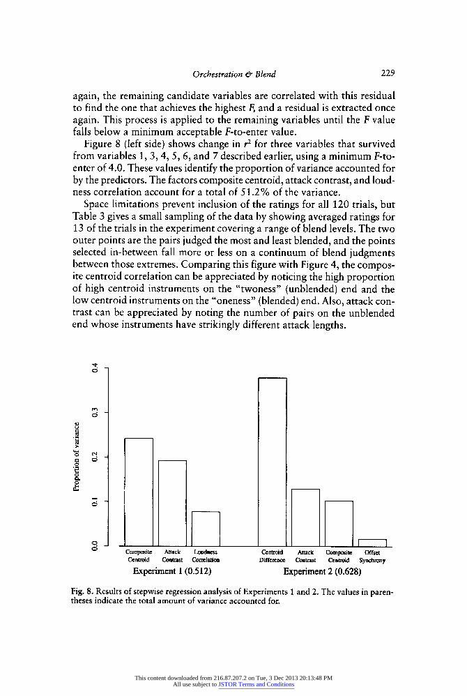
again, the remaining candidate variables are correlated with this residual to find the one that achieves the highest F, and a residual is extracted once again. This process is applied to the remaining variables until the F value falls below a minimum acceptable F-to-enter value.

Figure 8 (left side) shows change in r2 for three variables that survived from variables 1, 3, 4, 5, 6, and 7 described earlier, using a minimum F-to- enter of 4.0. These values identify the proportion of variance accounted for by the predictors. The factors composite centroid, attack contrast, and loudness correlation account for a total of 51.2% of the variance.

Space limitations prevent inclusion of the ratings for all 120 trials, but Table 3 gives a small sampling of the data by showing averaged ratings for 13 of the trials in the experiment covering a range of blend levels. The two outer points are the pairs judged the most and least blended, and the points selected in-between fall more or less on a continuum of blend judgments between those extremes. Comparing this figure with Figure 4, the composite centroid correlation can be appreciated by noticing the high proportion of high centroid instruments on the "twoness" (unblended) end and the low centroid instruments on the "oneness" (blended) end. Also, attack contrast can be appreciated by noting the number of pairs on the unblended end whose instruments have strikingly different attack lengths.

Fig. 8. Results of stepwise regression analysis of Experiments 1 and 2. The values in paren- theses indicate the total amount of variance accounted for.




Table 3 Thirteen Arbitrarily Selected Trials and Their Blend Ratings from the

120 Trials of Experiment 1

Instrument Pair Average Blend Rating

French horn and French horn .15 & French horn and bassoon .25 c Muted cello and trumpet .33 a Cello and flute .35 O Bassoon and soprano sax .38 ^ French horn and B clarinet .40 English horn and B clarinet .43 Muted trombone and bassoon .47 Muted trombone and bass clarinet .51 ^ English horn and flute .55 % Cello (sul ponticello) and alto sax .58 § Soprano and alto saxes .65 9 Alto sax and oboe .79 H

note. Trials were selected to show a range of variation of blend.

DISCUSSION

The appearance of composite centroid as the strongest predictor variable suggests that as the overall spectral centroid of the two instruments increases, the blend worsens. It does not seem to matter much whether the two instruments are close in centroid or not. This suggests the following heuristic: if both instruments are dark, blend should be maximal; but even if one of the two instruments is dark, the pair should blend better than if both are bright, since the dark instruments contributes to a lowering of the composite centroid. This is also consistent with Goodwin's (1989) findings that singers used an effectively darker tone when seeking to blend with one another. The appearance of the next strongest factor, attack contrast, con- firms the rather obvious expectation that attack asynchrony causes worse blend, and as shown in the findings of Rasch (1978, 1979). Finally, the appearance of the temporal loudness correlation factor is consistent with the notion of "common fate" from auditory grouping research: instruments with similar attack-sustain-decay characteristics will tend to blend with one another.

QUESTIONS

The "double-vowel" studies mentioned earlier showed that a strong degree of fusion (measured in terms of ability to recognize the component sounds in a pair) was obtained when sounds were on the same pitch, but that fusion decreased dramatically with small pitch separations (even less




that a semitone). Experiment 1, therefore, investigated blend where the sounds were already nearly optimal in their blend; indeed, most listeners reported that the task was hard because "they all blended." It would be useful to know how the patterns of blend change when there is no such advantage, and this is explored in Experiment 2. A pitch separation of three semitones, or a musical minor third, was chosen because the maximum advantage of fundamental frequency separation found in the double- vowel studies is three semitones, and Grey's tones can be altered to supply tones for this interval with a minimal number of transpositions.13 The use of an interval will now mean that instruments can be in different positions (e.g., there will be two versions of the pairing flute/oboe).

Experiment 2

STIMULI

Ten of the fifteen sounds used in Experiment 1 were used here: flute, oboe, englhorn, Bclar, bassclar, bassoon, frhorn, trumpet, normcello, and mutecello. Tones were arranged in pairs three semitones (minor third) apart using the pitches Cf4 and E4. Transposition to the two new pitches was achieved by wholesale shifting of frequency values. The perceptual changes caused by transposition were minimal, and the instruments' identities were satis- factorily preserved. All tones were equalized for presentation level by matching the overall root-mean-squared amplitude of the tones to one another; various listeners in the lab who compared the level of tones to one another reported that they sounded equally loud. Taking into account all pairs, with inversions and same-instrument pairings, there were 100 trials.

PROCEDURE

The task was identical to that of Experiment 1. Listeners were advised that the presence of two pitches would necessarily make the instruments more distinguishable, but that they should continue to rate the degree to which the aggregate sound suggested one or two timbres. Each listener rated the full set of 100 trials four times. The data for the seven retained listeners were averaged together into one block of 100 points.

RESULTS

One question of interest was whether the use of a new musical interval introduced new tendencies in the blend judgments, for example, if flute blended differently with Ek:lar depending upon whether it was above or below. One may speak of the two trials for flute/Ek:lar as being "inverse pairs." The mean rating difference between pairs of inversions was .087 (SE = .056), and the highest difference observed for a single pair of inver-

13. It may be noted that the tones have been transposed for use in other experiments (Grey, 1978) and for realizations of compositions (Erickson, 1974, as reported in Gordon, 1984, p. 2 and Erickson, 1982, p. 528).




sions was a mere .227 (Elclar-trumpet pair). These are very small differences, showing that inverse pairs obtained roughly the same amount of blend. Furthermore, similarity among the patterns of responses was checked by correlating groups of 10 inversionally related trials in which one of the instruments was constant (e.g., correlating the 10 trials with flute on Cf with the 10 trials with flute on E). The average correlation for the 10 possible pair-groups was r = .821 (p < .01, df= 8). Indeed, there appeared to be little difference in the ratings for inverse pairs, with the exception of a possible effect for the oboe: a t-test comparing the mean of all the trials in which oboe was on Cf4 (M = .366) to the mean of all the trials in which the oboe was on E (M = .456) showed a significant difference [£(18) = 2.232, p = .039], suggesting that the oboe blended better when on the bottom than on the top. Similar tests on all the remaining nine instruments, on the other hand, yielded nonsignificant results. Furthermore, the oboe finding is de- batable, because the presence of multiple tests requires the Bonferroni cor- rection (see Keppel, 1991); this effectively lowers the significance of the oboe £-test to p = .328. Therefore, the remaining analyses group all pairs of inversions together rather than analyzing them separately.

The nine factors used in the analysis of the results of Experiment 1 were also used here; the results for the two types of correlations are shown on the right side of Table 2. Centroid difference, not a strong factor in the previous experiment, played a much more significant role than in Experi- ment 1 (38% of the variance accounted for); the positive correlation indicates that blend worsened as the instruments in a pair were more distant in centroid.14 Although composite centroid correlates nearly as high as before, not all of the single-instrument correlations are positive, and the overall correlation is decidedly less than for centroid difference. Factors relating to transients are important once again: attack contrast is in fact slightly higher than before, and a role for offset synchrony has emerged. This latter correlation indicates that blend improved the more synchronously the aggregate of harmonics in a pair "turned off." The three temporal factors that were important in Experiment 1 (temporal centroid, loudness correlation, and harmonic synchrony) have either shrunk or disappeared in significance. A stepwise regression was applied to factors 1, 2, 5, and 9, as before (minimum F-to-enter = 4.0); in this case, all four factors were retained (accounting for 62.8% of the variance altogether) as shown in the right half of Figure 8.

14. The centroid difference correlation is preserved even when factoring out the changes in centroid due to the pitch shifts from B4 to Ci4 and E4. The possibility that the increased role for centroid difference in Experiment 2 is simply related to the increased pitch difference is remote, because the pitch shifts did not alter the centroid relationships between instruments in a consistent way: for many pairs, the distance was decreased, and for some, the sign of the difference was changed.




DISCUSSION

The absence of the factor of centroid difference in Experiment 1 and its emergence here raises the question of whether the separation of three semitones changed the way in which pairs were rated for blend. One hypothesis is that when the interval was a unison (Experiment 1), listeners did not compare the centroids of the two, but for a wider interval, they did. This may be a consequence of the increased pitch separation, which made the spectral features of each instrument more distinguishable, thus allow- ing the listeners to use this cue more reliably in making their blend judgments. This might also explain the disappearance of temporal factors (temporal centroid and loudness) from Experiments 1 to 2: that is, they did not provide any information beyond the cues provided by the now-enhanced spectral factors. Sensitivity to onsets is involved in roughly the same degree as before, but listeners show a sensitivity to offsets as well now.

Although it was clear from the listeners' comments that unisons blended far better in general, the two experiments were run several weeks apart and with only some of the listeners in common, so this difference is lost: listeners used the same range of blend ratings in Experiments 1 and 2. Kendall and Carterette (1993a) collected blend judgments for unison and nonunison conditions within a single experiment and found that the former blended much better; "double-vowel" studies show a pronounced advantage for unison intervals. It is highly probable that the same would have occurred in the present study if the two were run together.

The other interesting finding is the almost total lack of any effect for relative position of instrument. This is interesting because many of the pairs of inversions were easily distinguished from one another, and despite this, they tended to have the same degree of blend. Obviously, other instruments at other pitch separations would need to be tested before this finding could be extended to some general rule of orchestration.

QUESTIONS

Two experiments so far have shown aspects of centroid to be a primary factor in the judgments of blend. The factor of centroid was not manipulated independently, but was the fortuitous outcome of the fact that Grey's instruments represent a continuum of levels of centroid. To show centroid's contribution as an independent factor, however, it must be shown that when centroid alone changes, the blend increases or decreases according to the expected pattern. In the findings so far, one cannot rule out that the resulting blend judgments might have been due to confounding variables (e.g., other co-occurring acoustical factors of the instruments); after all, note how many diverse factors correlate in Table 2. The next experiment parameterized centroid so that individual instruments could be synthesized




with different centroids; this made it possible to explore the independent contribution of centroid to blend.

Additionally, manipulation of an amplitude condition was explored to see if this factor also has an independent effect on blend. Adjustments in amplitude are interesting because ensemble performers, when trying to obtain a blend among themselves, often adjust their dynamics to match one another in loudness. Usually the strategy is to make the louder instrument match the softer one (Scherchen, 1933, pp. 69-70). Considered together, the centroid and amplitude conditions are of potential interest. In real performance, centroid and amplitude level covary with performed dynamic variation: louder tones tend to be brighter, and softer tones tend to be darker. One can view the centroid and amplitude conditions as independent tests of the effect of these two aspects of dynamic variation on blend.

Experiment 3

STIMULI

The instruments flute, oboe, bassoon, and frhorn were selected for investigation because their centroids covered a large portion of Grey's tones' total range of centroids. Two sets of conditions were created: centroid and amplitude. For the centroid condition, the slope of the harmonic patterns was altered for each by applying a rate of attenuation or amplifica- tion (3 dB per octave) on the amplitudes of all the harmonics. This produced a "dark" and "bright" version of each of the tones, respectively. Normal versions of each instrument were created as well. Figure 9 shows the results of these transformations on the flute: in the dark version, upper harmonics were attenuated relative to the lower ones, whereas the reverse occurred for the bright version.

Instruments were synthesized on the pitches of Cf4 and E4, as in Experiment 2. Including the normal tones, this produced a total of 24 tones (4 instruments x 2 notes x 3 centroids), which were all equalized for root-mean-squared amplitude. The new and old centroids for all the tones are shown in Figure 10.

The reader will note that the differences between the centroids for the three levels of dark, normal, and bright within each instrument are not the same for all four instruments. The relationship between units of centroid in hertz and the corresponding amount of change in a perceptual attribute such as "brightness" or "sharpness" is a somewhat open question. A study by von Bismarck (1974b) presented evidence that an increase in the upper limiting frequency of a spectrum by seven critical bands corresponds to a doubling of sharpness. If this is true, what has been obtained in Figure 10 is in the right direction, because to achieve the same amount of perceptual change, a larger centroid change is necessary for a high- centroid instrument than for a low one. This nonlinearity became apparent during exploration of various methods for manipulating centroid while preparing the current experiment; for example, it was noticed that the 58-Hz difference between dark and normal centroid levels for frhorn (Figure 10) was nearly undetectable when applied to the oboe. A related problem is the fact that the flexibility with which the slope-changing approach can be applied is constrained by the fundamental frequency, number of harmonics, and native centroid of the tone to be modified. Consider, for example the pitch Cf, with a fundamental frequency of 277 Hz. The 300-Hz centroid change that is possible (and aurally acceptable) for the oboe (19 harmonics, centroid of 1084 Hz) is impossible for the French horn (11 harmonics, centroid of 475 Hz); the result of a -100-Hz change for the French horn, for



C <u

& X

PL]

c

I "3 o u r° 3 4-» G <v CJ

"03 >

M i <u

O

a D

03

<u

i nj

T3

|

I CD >

1




Fig. 10. A comparison of centroids for the instruments in the centroid condition of Experi- ment 3.

example, begins to approach a sine tone. Because the objective was to keep the identities of the instrument constant, this was unacceptable. The transformations of amplitude slopes described above, on the other hand, managed to preserve the naturalness or recognizability of the instrument sounds in a satisfactory way. The changes effected by centroid resembled transformations that a "treble" knob on a stereo amplifier would produce.

A second set of stimuli, with new amplitude levels, was synthesized for the amplitude condition. The same instruments, at both pitches, were synthesized with all harmonics attenuated equally by either 3 or 6 dB. Including the "normal" condition (0-dB attenuation), this produced a total of 24 tones.

PROCEDURE

Two sets of concurrent pairings were made, corresponding to the two conditions (centroid and amplitude). The following will describe how pairings were made, using the centroid condition as an example. Trials consisted of a pair of instruments playing the interval

Ct4-E4, as in Experiment 2. For a given pair of instruments (say, oboe on Cf, flute on E), there would be three trials in which one of the two notes would be in normal condition, and the other would vary between dark, normal, and bright. If the variable instrument was the flute, for example, these three trials would be oboe(normal)/flute(dark), oboe(normal)/ flute(normal), and oboe(normal)/flute(bright).

Although this "triad" of trials would appear nonconsecutively in the experiment (because trial orders were randomized), the goal was to observe how the changing level of centroid affected the judgments of blend. For instance, one might expect blend to worsen as the flute increases in centroid because the composite centroid becomes higher as a result.

Three further triads of trials were constructed with the same dyad: flute[E] kept "normal" with the oboe[Cf] varying in centroid, plus two other sets of triads equivalent to the two described so far, but with the instruments' pitch positions reversed. This produced,




when redundant "normal-normal" trials were eliminated, 10 trials for each instrument pairing. Same-instrument trials were not included in this experiment.

Each condition consisted of 24 triads, comprising a total of 60 trials when redundancies were eliminated. A harmonicity condition, also comprising 60 trials, was included in the stimulus set and judged for blend; it was later decided that these stimuli were not well designed for the purpose of exploring harmonicity, so their data will not be discussed further. Exploring all combinations of instruments, including the three conditions of centroid, amplitude, and harmonicity (discarded), and eliminating redundancies led to a total of 156 trials. Trials were presented in scrambled order (thus all the conditions were mixed together).

RESULTS

The data for the 10 retained listeners was averaged together into one block of 156 points; these were broken up according to the three conditions (60 trials each) and analyzed separately. The centroid condition will be analyzed first. First, the blend judgments for the centroid trials (N = 60) correlated overall both with composite centroid (r = .842, p < .0001, df = 58) and centroid difference (r = .709, p < .0001, df= 58), corroborating the results of the previous two experiments. More to the point, it is of interest whether such correlations occur within "triads" of pairs, where the instruments were held constant and only the centroids changed. From the previous evidence regarding composite centroid, it may be hypothesized that blend will successively worsen over the course of the dark, normal, and bright levels of centroid. With respect to centroid difference, on the other hand, it may be hypothesized that blend will successively worsen as the levels result in increasing centroid distance.

This was tested by arranging the three trials in a triad according to the increase in the factor and seeing if their corresponding blend values (x, y, and z) increased monotonically, that is, if the three blend ratings were in the relationship x < y < z. For example, for the triad shown in Table 4, x, y, and z would correspond to Trials 1, 2 and 3 (respectively) in the case of composite centroid, but Trials 3, 2, and 1 (respectively) for centroid difference. The blend ratings column shows how the findings are ultimately evaluated. Using the former ordering, blend judgments increase, but for the lat-

Table 4 Centroids and Blend Judgments for the Flute-Oboe Triad of Trials in

Experiment 3 to Illustrate the Analysis Procedure

Flute on Ct Frhorn on E Composite Centroid Blend Ratings Centroid (Hz) Difference (Hz)

T. Normal Dark 527 192 ^289 2. Normal Normal 534 154 .325 3. Normal Bright 548 102 .327




Table 5

Results for the f-Tests Used for Analyzing Experiment 3

Condition Slope Curvature

Composite Centroid M = .183 M = -.009 f(46) = 4.44 t{46) = -0.67 p < .001 * p = .504

Centroid Difference M = .181 M = -.018 ,(46) = 4.74 t(46) = -0.94 p < .001 * p = .358

Amplitude Hypothesis 1 M = .031 M = -.007 t(46) = -1.94 t(46) = -9.40

p = .064 p = .357

Amplitude Hypothesis 2 M = -.031 M = -.007 *(46) = 1.94 ^(46) = -9.40

/? = .064 p = .357

The tests "Slope" and "Curvature" refer to the degree to which the three blend judgments x, y, and z increased in the hypothesized order. Slope tests if z > x, and curvature tests if y falls between x and z. Asterisks indicate results with probabilities p < .05.

ter ordering, they do not, so effects for composite centroid but not centroid difference are found for this triad.

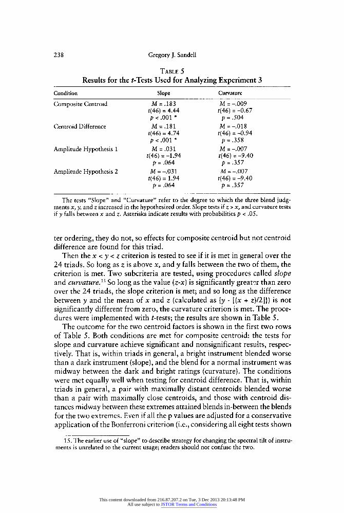
Then the x < y < z criterion is tested to see if it is met in general over the 24 triads. So long as z is above x, and y falls between the two of them, the criterion is met. Two subcriteria are tested, using procedures called slope and curvature. ,15 So long as the value (z-x) is significantly greater than zero over the 24 triads, the slope criterion is met; and so long as the difference between y and the mean of x and z (calculated as {y - [(x + z)/2]}) is not significantly different from zero, the curvature criterion is met. The procedures were implemented with t- tests; the results are shown in Table 5.

The outcome for the two centroid factors is shown in the first two rows of Table 5. Both conditions are met for composite centroid: the tests for slope and curvature achieve significant and nonsignificant results, respectively. That is, within triads in general, a bright instrument blended worse than a dark instrument (slope), and the blend for a normal instrument was midway between the dark and bright ratings (curvature). The conditions were met equally well when testing for centroid difference. That is, within triads in general, a pair with maximally distant centroids blended worse than a pair with maximally close centroids, and those with centroid dis- tances midway between these extremes attained blends in-between the blends for the two extremes. Even if all the p values are adjusted for a conservative application of the Bonferroni criterion (i.e., considering all eight tests shown

15. The earlier use of "slope" to describe strategy for changing the spectral tilt of instruments is unrelated to the current usage; readers should not confuse the two.




in Table 5 to be related), the still significant level p < .01 is obtained for the slope test. The mean slope value, averaged over both factors of centroid is .182, meaning that the mean difference in blend rating between adjacent levels of spectral centroid was nearly 20% of the rating scale; the maximum difference observed was nearly 50% of the blend scale. The results show that when centroid is manipulated independently of instrument, blend worsens (a) as the composite centroid gets higher and (b) as the difference in centroid between two instruments increases.

It was noted in the earlier discussion of the stimuli for this experiment that the amount of centroid changes between the levels dark, normal, and bright differed for the four instruments. The resulting changes in blend for these levels were proportional (correlation of r = .781): for example, the changes in blend judgments resulting from the French horn centroid changes were smaller than the changes in blend judgment for the analogous trials for the oboe, which had larger centroid changes. This suggests that the centroid steps were not perceptually equal across all the instruments. How- ever, this does not invalidate the basic test of whether blend judgments changed in the hypothesized direction as a result of changes in centroid.

Two hypotheses concerning the outcome of the amplitude condition were tested. Amplitude Hypothesis 1 is the idea that blend improves the closer two instruments are in loudness. This is consistent with a practice described by many musicians of "matching loudness" with another instrument to obtain a blend. Amplitude Hypothesis two is the idea that blend improves as one of the instruments becomes softer than the other. It is known that characteristic identifying features of instruments often become less salient when they are played softly, and a pair of instruments may achieve greater blend as the identity of the softer instrument is masked by the louder one (see timbre augmentation, earlier). Tests for these relationships were made using the same procedures as those for centroid. However, the results were null for both hypotheses, as shown in rows 3 and 4 of Table 5.

DISCUSSION

Whereas Experiments 1 and 2 were exploratory in nature and identified acoustical factors correlating with judgments of blend for pairs of instruments, Experiment 3 tested the hypothesis (along with others) that one of these factors (centroid) made an independent contribution to blend. The results do show that, even when only centroid is altered and everything else about the instrument is held constant, blend is a function of the composite centroid and/or the centroid difference of the pair: blend worsens as the composite centroid is made higher or the centroid difference is made larger. In contrast to the findings of Experiment 2, the effect was not stronger for centroid difference than composite centroid.




General Discussion

Blend for concurrently sounding musical instruments sounding on the same pitch could be explained in terms of three factors that accounted for 51% of the variance: the overall centroid height of the pair, the similarity of their attacks, and the similarity of their changes in loudness over time. When instruments were on different pitches separated by a minor third, 63% of the variance was accounted for by four factors: the difference in centroid between the two instruments, composite centroid, attack similarity, and synchrony of offset. In both, the centroid factors accounted for the largest proportion of this variance, and a third experiment confirmed that centroid made an independent contribution to blend by keeping instrument identities constant and manipulating their centroids.

The importance of closeness of centroid and attack patterns in this experiment is consistent with numerous other timbre studies that have shown them to be important for judgments of timbre similarity (Grey, 1975; Krumhansl, 1989; Iverson & Krumhansl, 1993; McAdams et al., in press; Wessel, 1979), timbre analogies (Ehresman & Wessel, 1978; McAdams & Cunible, 1992), and timbre streaming (Iverson, 1995) as well. The importance of combining like qualities in order to achieve a blend is stressed in orchestration writings (Adler, 1989, p. 472; Belkin, 1988, p. 50; Ott, 1969, p. 53; Russo, 1968, p. 562; Schoenberg, 1931/1975, p. 335; Stiller, 1985, p. 8).

The composite centroid factor suggests that a tone having strong high- frequency components possesses some advantage for segregation. This might be explained in terms of the distinguishability of spectral shapes in different frequency regions. In English vowels, first formants (FJ tend to be found in a small range (200-800 Hz) compared with the range in which second formants (F2) are found (800-2000 Hz). The bandwidths of these formants, on the other hand, are not nearly so dissimilar (F1 = 90 Hz, F2 = 110 Hz). Thus, in a concurrent pair of vowels, the locations of their Fxs are not as good a cue that two sounds are present than the locations of their P2s, because the two Fts are more likely to fall atop one another, whereas the F2s are more likely to be clearly distinguished. Thus having greater high-frequency information will lead to stronger F2s and thus greater segregation. If musical instrument spectra share such spectral features, this might explain the effect of composite centroid.

Another explanation for the advantage of bright sounds (composite centroid) for segregation is that higher frequency filters in the auditory system respond more slowly than lower frequency filters. Synchronies between harmonics would be more evident, then, when high frequencies were strong. Total harmonic synchrony was indeed a factor in Experiment 1 (although not in Experiment 2).




Conversely, composite centroid also means that a tone lacking in strong high-frequency components possesses some advantage for blend. This is consistent with Goodwin's (1989) "choral blend" findings, which showed that singers striving to attain a blend exhibit stronger fundamental frequencies and fewer and weaker upper partials than when singing in a solo manner. This factor is also widely confirmed in orchestration writings, which point out that conditions for blend are favorable when certain characteris- tically "dark" instruments are present: French horn (Piston, 1955, pp. 244, 365; Riddle, 1985, p. 51; Rimsky-Korsakov, 1912/1964, pp. 24, 35; Rogers, 1951, p. 104), bassoon (Adler, p. 210; Blatter, p. 112; Rimsky-Korsakov, 1912/1964, pp. 34-35), viola (Rogers, 1951, p. 26), and muted strings (Riddle, 1985, p. 124).

The centroid difference factor was found only for cases of nonunison pairings of instruments. Possibly the spectra were more indistinguishable at unison presentations so listeners relied more on temporal features, whereas when instruments were separated in pitch, the spectra were more distinguishable.

Instrument position did not seem to matter in nonunison pairs, for example, the blend obtained by flute-bassoon is more or less the same as that obtained by its inversional pair, bassoon-flute. In contrast, Kendall and Carterette (1993a) noted several differences between inversionally related pairs: for example, they observed that a group of instrument pairs classi- fied as "non-inverted" blended better as a group than their inversional counterparts. The assignment of pairs to the noninverted group appears to have been arbitrary, however, so it is unclear if the finding was fortuitous or related to some aspect of the instruments themselves. A correlation between their blend data and equivalent data of the present study is poor: r = -.272, p = .446 (using their figure 5). However, this can be explained by different number, pitch range, and characteristics of the instruments used in the two studies.

Only a small portion of a rather large problem has been explored in this study. In particular, the conclusions are constrained by the use of a limited number and pitch range of musical instruments, the fact that a few instruments were in unidiomatic registers, and the short, single-note presentations. However, the short, single notes may be sufficient to investigate blend. Kendall and Carterette (1993a) compared the blend of single-note presentations to richer contexts consisting of melodies in unison and nonunison (major third), but found that differences between contexts fell along unison versus nonunison lines, rather than single-note versus melody lines.

It is hoped that this study provided the beginning steps for a more modern approach to orchestration, by addressing the components of orchestration in terms of abstract attributes of musical sound. Teaching by example alone or with respect to one set of instruments ultimately renders an or-




chestration manual to a historical curiosity, as examples too easily reflect stylistic biases that rapidly become dated. With further research, it might be possible to teach orchestration in terms of acoustic properties such as the ones studied here (centroid, attack time, temporal similarity, etc.). The advantage of such a method is that it would be applicable to any musical sounds, acoustic or electronic, and could be used as a tool for analysis of orchestration as well.16'17

Appendix Problems Posed By Differences In Attack Time

The time at which a musical instrument tone is perceived to fall "on the beat" is not the same as the beginning of its attack. When musicians play in an ensemble, each musician delays or anticipates his or her time of physical onset relative to the conductor's downbeat to account for difference between native attack properties in the ensemble. Gordon (1984) termed the difference between the physical onset of sound in an instrument and the time of perceived downbeat as perceptual attack time (PAT).

When Grey's tones were aligned according to physical onset and combined in concurrent pairs for these experiments, many of the pairs sounded as though they were not attacked at the same time. An approximation of good ensemble playing, by adjusting the physical onsets of instruments in a pair, was desired so that the blend data would not be dominated by the too-obvious factor of attack difference. Such a simulation does not change any property of Grey's tone, it merely changes the times at which they begin relative to one another. The problem of arriving at some objective measure for simulating good ensemble timing was provided by Gordon (1984). Gordon studied the problem of PAT in a series of experiments in which listeners adjusted the interonset time of two successively presented instruments (looped repeatedly) until the instruments were perceived as isochronous. Gordon then modeled the results on the basis of the slope of the attack and the point at which the level of the tone crossed a threshold, resulting in a correlation of .995 between predicted and measured PAT. In all of the current experiments, each pair of instruments was adjusted for start time using the PAT values from Gordon's model.

16. This article is based on research that formed part of a Ph.D. dissertation (Sandell, 1991) submitted to Northwestern University. Some of the research was reported in previ- ously in Sandell (1989a, 1989b).

17. Support for Dr. Sandell was provided by Northwestern University (Committee on Interdisciplinary Research in the Arts), the Acoustical Society of America (F. V. Hunt Fel- lowship), a research grant in Experimental and Computational Studies of Human Cogni- tion (Science and Engineering Research Council, U.K.), and research grant number 5 P01 DC 00293-11 from the National Institute on Deafness and Other Communication Disor- ders, National Institutes of Health. My thanks go to Albert Bregman, Tom Carrel, Christo- pher Darwin, Zoltan Dienes, Toby Dye, Brian Glasberg, Gary Kendall, Roger Kendall, Jochen Krimphoff, Carol Krumhansl, Chris Plack, Steve McAdams, Trevor Shackleton, Stan Sheft, Alan Stout, David Wessel, and Bill Yost for their valuable advice, criticism, and assistance.

References

Adler, S. (1989). The study of orchestration (2nd éd.). New York: W. W. Norton. Assmann, P. F., ÔC Summerfield, Q. (1989). Modeling the perception of concurrent vowels:

Vowels with the same fundamental frequency. Journal of the Acoustical Society of America, 85, 327-338.




Assmann, P. F., & Summerfield, Q. (1990). Modeling the perception of concurrent vowels: Vowels with different fundamental frequencies. Journal of the Acoustical Society of America, 88, 680-697.

Beauchamp, J. W. (1982). Synthesis by spectral amplitudeand "brightness" matching of analyzed musical instrument tones. Journal of the Audio Engineering Society, 6, 396- 406.

Becker, H. (1969). The history of instrumentation. In K. G. Fellerer (Ed.), Anthology of music: A collection of complete musical examples illustrating the history of music (R. Kolben, Trans.). Cologne: A. Volk Verlag.

Belkin, A. (1988). Orchestration, perception, and musical time: A composer's view. Com- puter Music Journal, 12(2), 47-53.

von Bismarck, G. (1974a). Timbre of steady sounds: a factorial investigation of its verbal attributes. Acustica, 30, 146.

von Bismarck, G. (1974b). Sharpness as an attribute of the timbre of steady sounds. Acustica, 30, 159-172.

Blatter, A. (1980). Instrumentation/orchestration. New York: Longman. Brant, H. (1971). Orchestration. In J. Vinton (Ed.), Dictionary of contemporary music (pp.

538-546). New York: E. P. Dutton. Bregman, A. S. (1990). Auditory scene analysis. Cambridge, MA: MIT Press. Carlyon, R. P. (1991). Discriminating between coherent and incoherent frequency modula-

tion of complex tones. Journal of the Acoustical Society of America. 89. 329-340. Carse, A. (1964). The history of orchestration. New York: Dover. Chalikia, M. H., & Bregman, A. S. (1989). The perceptual segregation of simultaneous

auditory signals: Pulse train segregation and vowel segregation. Perception and Psychophysics, 46(5), 487-496.

Chalikia, M. H., & Bregman, A. S. (1993). The perceptual segregation of simultaneous vowels with harmonic, shifted, or random components. Perception and Psychophysics, 53(2), 125-133.

Cook, N. (1987). A guide to musical analysis. New York: George Braziller. Culling, J. E, & Darwin, C. J. (1993). Perceptual separation of simultaneous vowels: Within

and across-formant grouping by F0. Journal of the Acoustical Society of America, 93, 3454_3467.

Culling, J. E, & Summerfield, Q. (1995). The role of frequency modulation in the perceptual segregation of concurrent vowels. Journal of the Acoustical Society of America, 98, 837-846.

Darwin, C. J., & Carlyon, R. P. (1995). Auditory grouping. In B. C. J. Moore (Ed.), The handbook of perception and cognition: Vol. 6. Hearing (pp. 387-424). London: Aca- demic Press.

Darwin, C. J., Ciocca, V., & Sandell, G. J. (1994). Effects of frequency and amplitude modulation on the pitch of complex tone with a mistuned harmonic. Journal of the Acoustical Society of America, 95, 2631-2636.

Dixon, W. J. (1992). BMDP statistical software manual (Vol. 1). Berkeley: University of California Press.

Ehresman, D. L., ÔC Wessel, D. L. (1978). Perception of timbrai analogies (IRCAM Tech. Rep. 13). Paris: IRCAM.

Erickson, R. (1974). LOOPS: An informal timbre experiment (Tech. Rep. Q-037). Center for Music Experiment, University of California at San Diego, La folia, California.

Erickson, R. (1975). Sound structure in music. Berkeley: University of California Press. Erickson, R. (1982). New music and psychology. In D. Deutsch (Ed.), The psychology of

music (pp. 517-536). New York: Academic Press. Goodwin, A. W. (1989). An acoustic study of individual voices in choral blend. Journal of

Research in Singing, 13(1), 25-34. [Reprinted from The Journal of Research in Music Education, 1980,25(2), 119-128.1

Gordon, J. W. (May 1984). Perception of attack transients in musical tones. Doctoral dissertation, Stanford University, Stanford, CA. Issued through the Department of Music, Center for Computer Research in Music and Acoustics, Report no. STAN-M-17.




Gordon, J. W. (1987). The perceptual attack time of musical tones. Journal of the Acousti- cal Society of America, 82, 88-105.

Grey, J. M. (1975). An exploration of musical timbre. Doctoral dissertation, Stanford Uni- versity, Stanford, CA. Issued through the Department of Music, Center for Computer Research in Music and Acoustics, Report no. STAN-M-2.

Grey, J. M. (1977). Multidimensional scaling of musical timbres. Journal of the Acoustical Society of America, 61, 1270-1277.

Grey, J. M. (1978). Timbre discrimination in musical patterns. Journal of the Acoustical Society of America, 64, 467-472.

Grey, J. M., & Gordon, J. W. (1978). Perceptual effects of spectral modifications on musical timbres. Journal of the Acoustical Society of America, 63, 1493-1500.

Grey, J. M., & Moorer, J. A. (1977). Perceptual evaluation of synthesized musical instrument tones. Journal of the Acoustical Society of America, 62, 454-466.

Iverson, P. (1995). Auditory stream segregation by musical timbre: Effects of static and dynamic acoustic attributes. Journal of Experimental Psychology: Human Perception and Performance, 21, 751-763.

Iverson, P., ÔC Krumhansl, C. L. (1993). Isolating the dynamic attributes of musical timbre. Journal of the Acoustical Society of America, 94, 2595-2603.

Jones, D., Kendall, G., ÔC Martens, W. (1984). Designing a sound room for auditory research using the TEF™. Poster presented at the 1984 International Computer Music Conference.

Kendall, R. A., & Carterette, E. C. (1993a). Identification and blend of timbres as a basis for orchestration. Contemporary Music Review, 9, 51-67.

Kendall, R. A., 8t Carterette, E. C. (1993b). Verbal attributes of simultaneous wind instrument timbres: I. von Bismarck's adjectives; II. Adjectives induced from Piston's orchestration. Music Perception, 10, 445-468, 469-502.

Keppel, G. (1991). Design and analysis: A researcher's handbook. Englewood Cliffs, NJ: Prentice-Hall.

Koury, D. J. (1986). Orchestral performance practices in the nineteenth century. Ann Ar- bor, MI: UMI Research Press.

Krumhansl, C. L. (1989). Why is timbre so hard to understand? In S. Nielzén & O. Olsson (Eds.), Structure and perception of electroacoustic sound and music (pp. 43-53). Amsterdam: Excerpta Medica.

Lerdahl, E (1987). Timbrai hierarchies. Contemporary Music Review, 2, 135-160. McAdams, S. (1984). Spectral fusion, spectral parsing and the formation of auditory im-

ages. Doctoral dissertation, Stanford University, Stanford, CA. Issued through the De- partment of Music, Center for Computer Research in Music and Acoustics, Report no. STAN-M-22. .

McAdams, S. (1989). Concurrent sound segregation. I: Effects of frequency modulation coherence. Journal of the Acoustical Society of America, 86, 2148-2159.

McAdams, S., & Cunible, J.-C. (1992). Perception of timbrai analogies. Philosophical Trans- actions of the Royal Society of London, 336, 383-389. [Also in Carlyon, R. P., Darwin, C. J., & Russell, I. J. (Eds.), Processing of complex sounds by the auditory system (pp. 89-95). Oxford: Clarendon Press.]

McAdams, S., & Saariaho, K. (1985). Qualities and functions of musical timbre. Proceed-

ings of the 1985 International Computer Music Conference (pp. 367-374). San Fran- cisco: The Computer Music Association.

McAdams, S., Winsberg, S., Donnadieu, S., De Soete, G., & Krimphoff, J. (in press). Per-

ceptual scaling of synthesized musical timbres: common dimensions, specificities, and latent subject classes. Psychological Research, 58.

Moore, B. C. J. (1986). Frequency selectivity in hearing. London: Academic Press. Moore, B. C. J., ÔC Glasberg, B. R. (1983). Suggested formulae tor calculating auditory-

filter bandwidths and excitation patterns. Journal of the Acoustical Society of America, 74y 750-753.




Moore, B. C. J., & Glasberg, B. R. (in press). A revision of Zwicker's loudness model. Acustica

Moorer, J. A. (1973). The heterodyne method of analysis of transient waveforms (Tech. Rep.). Stanford, CA: Artificial Intelligence Laboratory, Stanford University.

Moorer, J. A. (1985). Signal processing aspects of computer music: A survey. In J. Strawn (Ed.), Digital audio signal processing: An anthology. Los Altos, CA: W. Kaufmann.

Moorer, J. A., & Grey, J. (1977). Lexicon of analyzed tones: Part I. A violin tone. Computer Music Journal, 1(2), 39-45.

Moorer, J. A., Grey, J., ÔC Strawn, J. (1977). Lexicon of analyzed tones: Part II. Clarinet and oboe tones. Computer Music Journal, 1(3), 12-29.

Moorer, J. A., Grey, J., 8c Strawn, J. (1978). Lexicon of analyzed tones: Part III. The trumpet. Computer Music Journal, 2(2), 23-31.

Ott, J. (April 1969). A new approach to orchestration. The Instrumentalist, 23(9), 53-55. Piston, W. (1955). Orchestration. New York: Norton. Rasch, R. A. (1978). The perception of simultaneous notes such as in polyphonic music.

Acustica, 40, 21-33. Rasch, R. A. (1979). Synchronization in performed ensemble music. Acustica, 43, 121-

131. Riddle, N. (1985). Arranged by Nelson Riddle. Secaucus, NJ: Warner Brothers. Rimsky-Korsakov, N. (1964). Principles of orchestration (E. Agate, Trans.). New York:

Dover. (Original work published 1912) Risset, J., & Wessel, D. (1982). Exploration of timbre by analysis and synthesis. In D.

Deutsch (Ed.), The psychology of music (pp. 25-88). New York: Academic Press. Rogers, B. (1951). The art of orchestration: Principles of tone color in modern scoring.

New York: Appleton-Century-Crofts. Russo, W. (1968). Jazz composition and orchestration. Chicago: Universitv of Chicaeo Press. Sandell, G. J. (1989a). Perception of concurrent timbres and implications for orchestration.

In Proceedings of the 1989 International Computer Music Conference (pp. 268-272). San Francisco: Computer Music Association.

Sandell, G. J. (1989b). Effect of spectrum and attack properties on the evaluation of concurrently sounding timbres. Journal of the Acoustical Society of America, #6(Suppl. 1 ), S89. Abstract of presentation to the 118th Meeting of the Acoustical Society of America, St. Louis, October 1989.

Sandell, G. J. (1991). A library of orchestral instrument spectra. In Proceedings of the 1991 International Computer Music Conference. San Francisco: The Computer Music Asso- ciation.

Sandell, G. J. (1995). The SHARC timbre database. World Wide Web URL: <http:// www.parmly.luc.edu/sharc> (electronic publication).

Scheffers, M. T. M. (1979). The role of pitch in perceptual separation of simultaneous vowels. IPO Progress Report, 14, 51-54.

Scheffers, M. T. M. (1983). Sifting vowels: auditory pitch analysis and sound segregation. Doctoral dissertation, Groningen University, The Netherlands.

Scherchen, H. (1933). Handbook of conducting. London: Oxford University Press. Schoenberg, A. (1978). Theory of harmony (Roy E. Carter, Trans.). Berkeley: University of

California Press. (Original work published 1911) Schoenberg, A. (1975). Instrumentation. In L. Stein (Ed), Style and idea (pp. 330-336).

New York: St. Martin's. (Original work published 1931) Slawson, A. W. (1985). Sound color. Berkeley: University of California Press. Stern, R. M. (July 15 1972). Perception of simultaneously presented musical timbres (Tech.

Rep.). Massachusetts Institute of Technology, Research Laboratory of Electronics, Cam- bridge, Massachusetts Quarterly Progress Report, pp. 202-210.

Stiller, A. (1985). Handbook of instrumentation. Berkeley: University of California Press. Varèse, E. (1967). New instruments and new music. In E. Schwartz & B. Childs (Eds.),

Contemporary composers on contemporary music (pp. 196-198). New York: Holt,




Rinehart & Winston. (Lecture given at Mary Austin House, Santa Fe, New Mexico, 1936)

Wessel, D. L. (1979). Timbre space as a musical control structure. Computer Music Jour- nal 3, 45-52.

Zwicker, U. T. (1984). Auditory recognition of diotic and dichotic vowel pairs. Speech Communication, 3, 265-277.



Roles for Spectral Centroid and Other Factors in...

Documents

Transcript of Roles for Spectral Centroid and Other Factors in...