Rockfall Hazard Assessment in Gunung Kelir Area Yogyakarta...

Memoirs of the Faculty of Engineering, Kyushu University, Vol. 74, No. 2, September 2014

Rockfall Hazard Assessment in Gunung Kelir Area Yogyakarta, Indonesia

by

Guruh SAMODRA*, Guangqi CHEN** , Junun SARTOHADI ***

and Kiyonobu KASAMA†

(Received July 23, 2014)

Abstract

Rockfall hazard assessment should be treated in a different way compared to

other mass wasting phenomena due its complex nature. Rockfall hazard

assessment involves determination of rockfall source, size-frequency, onset

susceptibility, temporal probability and deposit area. In this paper, we propose a

methodological framework of rockfall hazard assessment which is expected to

answer "where", “how frequent” and “how large” rockfall are likely to occur.

Rockfall inventory and frequency-size analysis are employed to assess temporal

distribution, size and frequency of rockfall which may occur in the future.

GIS-lumped mass rockfall simulation is employed to identify potential rockfall

source based on the distribution of boulders from the past rockfall events. And

then, reliable trajectories are estimated once the potential rockfall sources are

identified. It represents the rockfall susceptibility degree in the study area. Since

GIS-lumped mass model does not consider the size, shape and fragmentation of

the boulder, 2D DDA is employed to analyze the trajectory which has a potency

of high risk, e.g. trajectory passing a building. Information of rockfall hazard

represented as the susceptible location and magnitude-frequency, including

temporal probability of rockfall can be further employed to formulate an

appropriate landuse planning in a rockfall prone area.

Keywords: Rockfall, Hazard, GIS, DDA, Frequency-magnitude

1. Introduction

The word rockfall is often distinguished from more general landslide phenomena due its typical

material, size and failure mechanism. It is defined as rock fragments1) with size from a few dm3 to

104 m3 2) started by the detachment of blocks from their original position3) and followed by free

falling, bouncing, rolling or sliding 4). As a consequence, determining rockfall hazard will not be

simple to achieve in practice3) due to its complex nature. Rockfall hazard assessment involves

determination of rockfall source, size-frequency, spatial probability/onset susceptibility, intensity,

and deposit area.

* Graduate Student, Department of Civil and Structural Engineering ** Professor, Department of Civil and Structural Engineering *** Professor, Department of Environmental Geography Universitas Gadjah Mada † Associate Professor, Department of Civil and Structural Engineering

38 G. SAMODRA, G. CHEN, J. SARTOHADI and K. KASAMA

Identification of potential rockfall source in medium to large scale mapping is one of the main

difficulties in rockfall hazard assessment5). Several authors have proposed simple empirical

threshold angles for potential rockfall source such as slope >45°6), slope >60°7) and slope >37°8).

Recent methods are by combining several parameters such as slope angle, discontinuity, curvature,

slope scree, distance to fault, block size9), geology and rock condition, slope, ditch dimension,

seepage, event history10); by using DEM-based geomorphometric analysis5); and by employing

terrestrial laser scanner11).

Size-frequency is usually based on the rockfall inventory data. However, complete inventory

data are not available in many developing countries. Most complete inventory data are available in

developed country e.g. Grenoble French Alps, French2), Yosemite California, USA12,7) and British

Columbia, Canada 13). Several laws for frequency-magnitude of rockfall have been successfully

proposed by Hungr et al.13) and Dussauge et al.14) because of the availability of complete historical

data. However, the major limitations to size-frequency analysis include the lack of rockfall

inventories for most sites and the spatial and temporal heterogeneity of available inventories.

Rockfall spatial probability/onset susceptibility employed several approaches such as GIS

(Geographic Information System) susceptibility mapping, numerical simulations and full scale

experiment15). The application of rockfall susceptibility assessment usually depends on the scale of

the area. GIS susceptibility mapping is usually applied in regional scale, whereas numerical

simulations and full scale experiment are applied in a limited area or large scale. Most spatial

probability approaches include intensity analysis, i.e. velocity and energy.

GIS susceptibility mapping is a powerful tool to assess spatial probability of rockfall in regional

scale (large area). It is based on Digital Terrain Model (DTM) representing topography in raster

format. The model is very powerful to simulate the physical characteristics of the surface rather

than the physical characteristic of the boulder itself. The additional attribute related to geology,

land use or vegetation type and rock type represented in spatial data can also be included in the

model. GIS model is able to determine the trajectory of rockfall movement, the deposit area and the

potential intensity of rockfall. However, GIS models usually use lumped mass approach16). It means

that the boulder of rockfall is dimensionless; without considering the size, shape and mass of the

boulder.

Numerical rockfall simulation such as DDA17) is able to represent rockfall more realistic. The

contact forces are calculated during the interaction between boulder and slope. Modeling the

dynamic displacement and deformation of an elastic body in any shape are the advantages of the

DDA. It includes the rigid body displacement, rotation and deformation of a block. Reliable

trajectory and dynamic behavior of boulder when travel along the slope are also able to be

identified based on the characteristic of material, shape and size. However, DDA simulation will be

more complex, need excessive computational requirements16) and time consuming when it is

applied in large area or regional scale.

Rockfall threat in Gunung Kelir is one of the main concerns in Kulon Progo local government.

Several rock fragments fell down through the colluvial foot slope and18). PSBA UGM19) conducted

a preliminary qualitative hazard assessment to provide guidance on the design of rockfall measures

for the local government. It involves expert judgement on the potential occurrence of rockfall

hazard based on geomorphological survey and the position of element at risk. The qualitative

hazard assessment was the only possible approach employed at that time due to the limited time

and the absence of available rockfall data.

This paper is aimed to propose an additional hazard analysis for better understanding of rockfall

hazard containing susceptibility, size-frequency and temporal probability. It involves

frequency-volumes statistics of rockfall deposits inventory, spatial trajectories of potential rockfall

Rockfall Hazard Assessment in Gunung Kelir Area Yogyakarta 39

and simulating physical mechanism of rockfall displacement and deformation in the trajectory

which has a potency of high risk. In addition, impact force analysis is also performed to infer the

physical vulnerability of element at risk in a specific scenario.

2. Study Area

Gunung Kelir is located in the western part of Yogyakarta Province, Indonesia (Fig. 1). It lies in

the upper part of Menoreh Dome that is located in central part of Java Island. The area is dominated

by Tertiary Miocene Jonggrangan Formation that consists of calcareous sandstone and

limestone. Bedded limestone and coralline limestone which form isolated conical hills may

also be found in the highest area surrounding study area. Weathering, erosion, and mass

movement are common geomorphological processes in the study area. Gunung (Mountain) Kelir,

of Javanese origin, literally means a curtain that is used to perform wayang (Javanese

traditional puppet). Its toponym describes a 100-200 meter high escarpment that has slope

nearly 90°.

Fig. 1 (a) Map of Indonesia with the red box indicates Java Island (b) Gunung Kelir Area is located in the

middle part of Java Island (c) DEM of Menoreh Dome with the red box indicates Gunung Kelir Area (d)

3D view of Gunung Kelir Area with building and main road.

The escarpment is a product of the final uplifting of the Complex West Progo Dome in the

Pleistocene20). The slope gradient of escarpment varies between 50° and 80°, meanwhile mean

of slope gradient is 23.14°. The elevation ranges from 600 to 837.5 m. There are 152 buildings

exposed as element at risk in the lower slope of the escarpment.


3. Methodology and Data Collection

3.1 Rockfall Inventory and Frequency-Size

Rockfall inventory is a key issue for frequency-size analysis. Research on rockfall hazard is

more challenging in developing country such as Indonesia where no available rockfall catalogue is

present. Inventory of rockfall boulder/deposits must be carried on by intensive fieldwork to infer

the probability distribution of rockfall size. Recently, several techniques of landslide inventory

mapping are developed well, such as aerial photo interpretation21, 22, 23, 24), surface morphology

interpretation of very high resolution DEM10,25,26 ,27) and interpretation of satellite imagery28, 29,30).

However, it is rather difficult to be applied in rockfall inventory mapping. For example, the rockfall

size in Gunung Kelir area is 31.57 m3 in average, meaning too small to be interpreted by imagery

analysis.. In addition, high density of a canopy layer may reduce the visibility of rockfall boulder

below the vegetation layer from imagery data. Thus, extensive geomorphology inventory with

transect walk was carried on to plot 521 rockfall boulders in Gunung Kelir area. Coordinate

location was recorded by GPS (Global Positioning System) and the size of a boulder was measured

by laser rangefinder. Then, all data obtained from fieldwork are transferred into GIS environment.

The temporal probability of rockfall can be inferred from the magnitude-frequency distribution.

It was derived from magnitude-cumulative frequency (MCF) curves constructed from rockfall

inventory using graphical method2,13). Magnitude-cumulative frequency curve was generated by

sorting the volume of rockfall and accumulating the incremental frequencies from largest to

smallest. It was inferred that the length in years of the total of 521 boulders in the entire area is 141

years. The resulting magnitude-cumulative frequency (MCF) plot is shown in Fig. 2.

Fig. 2 Magnitude-cumulative Frequency (MCF) Curve

However, the cumulative frequency or incremental frequency is sometime difficult to be

employed directly as temporal probability in the hazard analysis. Small volume boulder can have

incremental frequency more than 1 (Fig. 2 and Table 1). It means that rockfall may occur once or

more in each year in a given volume. It does not represent a probability value ranging from 0 to 1.

Thus, Poisson probability was employed to calculate the temporal probability of rockfall with the

volume in a given volume class.


Table 1 Number of Boulders in each Volume Class in Gunung Kelir Area.

Year = 141 Vol class Number Incremental freq.

<10 352 2.50

10-100 137 0.97

100-1000 29 0.21

>1000 3 0.02

The temporal probability of rockfall was calculated from the observation of the frequency of the

past event and MCF relation. It is defined as a percent chance of one or more rockfall in a given

volume falling during specified time. It is similar to the hydrology analysis. In this case, rockfalls

were treated as recurrent events that occur randomly and independently. Actually, this assumption

does not fully accepted because once the rockfall occurs, it may change the slope morphometry

which can affect the independency of future events. However, given a certain lack of understanding

the physical process on the changing morphometry that control rockfall, Poisson model is one of

feasible method to estimate the temporal probability of rockfall events.

There were 16 rockfall events reported by eyewitnesses during 1970-2009 (16 events during

period of 39 years) in the lower slope where the total number observed by geomorphological

mapping are 58. The rockfall inventory data were collected and documented from field survey

which is calculated in the 141-year period (521 rockfall events). The main assumption of temporal

probability of rockfall is that rockfall can be considered as independent random point-events in

time. The probability of rockfall occurrence during time t is:

[ ]1)( ≥= tNPPN (1)

where N(t) is the number of rockfalls that occur during time t in the investigated area.

Probability model is commonly used to investigate the occurrence of independent random

point-events in time i.e. Poisson model. The Poisson model considers naturally continuous rockfall

data.

[ ]!

)()exp()(

n

ttntNP

nλλ−== n=0,1,2,.... (2)

where P[N(t) = n] is the probability of experiencing n landslides during time t, λ is the

estimated average rate of occurrence of rockfalls which corresponds to 1/µ, with µ is the estimated

mean recurrence interval between successive failure events. The variable λ and µ can be obtained

from a historical catalogue of landslide events or from a multi-temporal landslide inventory map.

The probability of experiencing one or more rockfalls during time t (exceedance probability) as

follows:

[ ] [ ] ttNPtNP λ−−==−=≥ exp10)(11)( (3)

[ ] µ

t

tNP

−

−=≥ exp11)( (4)

By adopting a Poisson model (eq. 4), the author computed the exceedance probability of having

one or more rockfall in each landform (Table 2).

3.2 Potential Source Area Identification

The potential rockfall source area was identified by thematic map analysis. Identification of


potential rockfall source was identified by thematic map analysis, e.g. landuse and threshold of

slope (Fig. 3). Shrub and outcrop are the most potential area being rockfall source, whereas

farm/plantation is less potential area being rockfall source. Some farmer plant Teak (Tectona

Grandis), Pinus Mercusi, Agathis Alba, Maleleuca sp., and Dalbegia Latifolia in the farm/plantation

landuse type. Based on the empirical experience in Gunung Kelir area, slope threshold >55 degree

was determined as a potential rockfall source area. The overlay technique of spatial thematic data

(e.g. landuse and slope) and analysis of cracking, lithology were employed to determine the

potential rockfall area. Once the rockfall trajectory has been simulated, the potential rockfall source

was also compared to the boulder deposits obtained from geomorphology inventory.

Fig. 3 (a) Landuse Map (b) Slope Map (c) Boulder Deposits from Inventory Mapping (d) Potential

Rockfall Source.

3.3 Rockfall Susceptibility Analysis

3.3.1 GIS Rockfall Analyst

GIS modeling based on lumped mass32) was applied to model the trajectory and velocity of

rockfall along the escarpment of Gunung Kelir Indonesia. It considers the dynamic process of

rockfall based on the cell plane obtained from raster based Digital Elevation Model (DEM). DEM

represents the earth surface or topography containing actual height points. GIS can produce various

topographic parameters (derivative of DEM) such as slope, aspect, curvature easily. In GIS


Rockfall analyst, the DEM derivatives, i.e. slope angle and aspect angle are used to construct the

normal vector of each cell plane32). It is expressed in the global Cartesian system as:

un = (sin θ sin φ, sin θ cos φ, cos θ) (5)

where un unit normal vector, θ is the slope angle and φ is the aspect angle.

To reduce the excessive computational requirements in a GIS environment, rockfall analyst

employs lumped mass approach to assess the trajectory and velocity of rockfall. It means that the

rockfall simulation will not consider the size and shape of the boulder. The rockfall process

including the modeling of free falling, bouncing and rolling or sliding is performed by discrete time

steps. It is automatically determined by both cell size and particle velocity. Physical quantity of

boulder such as rock position, displacement, velocity, acceleration, force and momentum is

represented in 3D vector space. For instance, the flying path of boulder computed by parabolic

equation is defined as

�̅ = � 00−�� + �� + �� (6)

where g is the acceleration due to gravity (9.8 m/s2), X0, Y0, Z0 is the initial position and Vx0, Vy0,

Vz0 is the initial velocity of the rock in x, y, z direction. Whereas, the velocity vector of the rockfall

is defined as

�̅ = � �� − � = � 00−� + �� (7)

In addition, coefficient restitution is also included to calculate the bouncing velocity in the

intersection location between flight path parabola and the grid cell surface. It involves coefficient

of normal restitution RN and coefficient of tangential restitution RT. The bouncing velocity vector in

a local coordinate system is defined as

V’Dip = VDipRT (8)

V’Trend = VTrend RT (9)

V’N = VNRN (10)

where VDip is the velocity components of rock in the dip direction, VTrend is the velocity components

of rock in the trend direction, VN is the velocity components in normal direction of slope cell.

Beside projectile algorithm for falling, the rolling or sliding algorithm is also determined by the

interaction between rock velocity vector and the normal vector of cell plane32).

Table 2 Properties of Surface Material (Adopted from Rocscience website, 2014).

Surface Types RN RT

Sandstone face 0.53 0.9

Vegetated soil slope 0.28 0.78

Soft soil, some vegetation 0.30 0.3

Limestone face 0.31 0.71

Talus cover with vegetation 0.32 0.8

However, GIS-lumped mass model is dimensionless, meaning that it does not consider the size,

shape and fragmentation of the boulder. The more mechanically numerical rockfall simulation is

needed as a complementary tool to analyze the trajectory which has a potency of high risk, e.g.

trajectory passing a building. It should be able to model the dynamic displacement and deformation


of an elastic body in any shape and consider the rigid body displacement, rotation and deformation

of a block. Thus, 2D DDA was employed to confirm the reliable trajectory and dynamic behavior

of boulder when travel along the slope having high risk possibility.

3.3.2 2D DDA

Extended 2D DDA33) was employed to assess the motion behavior of the most dangerous

rockfall trajectory obtained from GIS modeling. DDA is one of numerical simulation that can be

applied to simulate the motion behavior of rock. It deals with the problem of rigid body movement

and large deformation of a rock block system under general loading and boundary17). Even though

DDA is parallel to finite element, the advantage of 2D DDA is that every single block can be

convex or concave in two dimensional polygon. In addition, Coulomb’s law is applied to the

contact interface and the simultaneous equilibrium equations are solved for each loading or time

increment34). Each block can interact and deform independently.

There are six displacement variables working in DDA when a block experiences constant

stresses and constant strains throughout35). The displacement (u,v) of any point (x,y) of a block can

be defined as six variables as follows:

(u0 v0 r0 εx εy γxy) (11)

where u0,v0 are the parallel translation (u,v) of a specific point (x0,y0) on the block; r0 is the rotation

angle (in radians) of the block with the rotation center at (x0,y0). εx εy γxy are the normal and shear

strains of block at (x0,y0). Displacements (u,v) of the point (x,y) containing several mechanisms

such as parallel translation, rotation, normal strain and shear strains are formulated separately.

Thus, the total displacement (u,v) of the same point (x,y) is the accumulation of displacements

induced by six variables (Shi, 1988) . It can be defined as:

�� = �1 00 0−� − �! �� − ��!�� − ��! 0 0 � − �!� − �! �� − ��!"#$$$$%��&�ε�ε�γ'()*

***+ (12)

2D DDA model will take an advantage of a GIS model to simulate the motion behavior of the

boulder. 2D slope profile from DEM was imported to the 2D DDA to draw rock block system and

to simulate the contact force of multiple falling rock. The displacement behavior of each block in

the dynamic simulation can be traced and can be seen at the end of each calculation step.

3.4 Rockfall Hazard Assessment

Hazard in term of landslide is often defined as an estimation of spatial distribution/susceptibility,

temporal distribution, size and frequency of landslide which may occur in the future. The

information should include the location, size (volume) and velocity of the potential landslides and

any resultant detached material and the probability of their occurrence within a given period of

time36). Rockfall hazard assessment is expected to answer “where”, “how frequent” and “how large”

rockfall are likely to occur which are not taken into account in landslide susceptibility zoning.

However, conducting rockfall hazard assessment that fully complies the rockfall definition is still a

challenge and will not be simple to achieve in practice. In this paper, we proposed a methodological

framework of rockfall hazard assessment (Fig. 4), i.e. identifying the release/potential source,

path/trajectories, depositional area, temporal probability, and rockfall intensity. This can bridge the

gap between a statistical method which only predict where rockfall will occur in the future based

on past inventory and deterministic method which usually analyze rockfall based on simple


mechanical laws and usually applied in limited areas.

Fig. 4 Methodological Framework of Rockfall Hazard Assessment.

Rockfall hazard (spatial, temporal and magnitude) was defined by integration of

geomorphology suvey, statistics and GIS-spatial analysis. Geomorphology survey of rockfall

boulders and semi structured interview were conducted to determine the magnitude probability and

temporal probability of rockfall. Frequency magnitude analysis of rockfall volume was calculated

by observing the cumulative frequency distribution in log-log chart. The size-volume data was used

as an input in 2D DDA in order to obtain motion behavior of the most dangerous rockfall trajectory.

The spatial probability of rockfall was described by potential trajectory along the sub-vertical cliff. The result of potential trajectory is controlled by the geomorphology inventory of rock boulder/deposits and spatial analysis of rockfall source. Spatial probability containing the release/potential source, path/trajectories, depositional area has been firstly defined. The most dangerous rockfall trajectory is chosen from the result of the GIS trajectory

model. Then, the slope profile of the most dangerous rockfall trajectory and rockfall size

distribution are used as input for 2D DDA to compute displacement, rotation and deformation of a

block. Thus, the proposed methodological framework does not only provide quantitative input data

for the estimation of future risk, but also important for policy making to assist establishment of

structural and or nonstructural preventive measures including landuse planning by considering the

spatial, temporal and intensity distribution of rockfall occurrence.

4 Results and Discussions

4.1 Temporal Probability

Beside geomorphology inventory, we also conducted semi closed questionnaire interviews to

obtain the temporal data of rockfall occurrences. We found that 16 rockfall occurrences have been


observed by eyewitness during 1970-2009. The temporal information was combined with

frequency magnitude analysis to obtain probability occurrence of a given volume in a given time

period in a given area. The temporal probability is described by the chance one or more rockfall

during specified time.

The temporal information applies for hazard assessment in Gunung Kelir. Based on the

equation (3) and (4), rockfall in each volume class has a chance of one or more rockfall during a

specified time for an area 0.12 km2. It shows that the smaller volume will have higher chance to

occur in a specified time (Table 3).

Table 3 Poisson Model for Percent Chance One or more Rockfall on each Volume Class, during Specified

Time.

Volume

Class

Number

per Class

Chance of one or more rockfall during specified time

1 yr. 5 yrs. 10 yrs. 25 yrs. 50 yrs. 100 yrs. 141 yrs.

<10 352 0.92 1.00 1.00 1.00 1.00 1.00 1.00

10-100 137 0.62 0.99 1.00 1.00 1.00 1.00 1.00

100-1000 29 0.19 0.64 0.87 0.99 1.00 1.00 1.00

>1000 3 0.02 0.10 0.19 0.41 0.65 0.88 0.95

4.2 Rockfall Hazard in Gunung Kelir

The calculation of GIS rockfall modeling is represented by vector format. It shows trajectories

along the escarpment. The starting point of boulder is treated as a seeder location in the convex

creep slope. The potential rockfall source area was identified by field survey and thematic map

analysis. Sampling distance for seeder along the source area was set as 5 m. The simulation of rock

fall trajectory predicts how far a boulder passes through slope. Bouncing, falling, rolling or sliding

including the velocity are also able to be investigated in each trajectory. It describes that highest

velocity is attained before the end of rock’s flight. The potential rockfall source area as polyline

seeder were positioned separately based on the pattern of boulder deposition and slope direction.

Coefficient of surface parameters (Table 2) was also used to control boulder movement during

impact at the end of rock flight. The result of trajectory model is also compared to the boulder

deposition obtained from GPS plotting and fieldwork activities. The trajectory stop point is good in

agreement with the boulder deposition in GIS model.

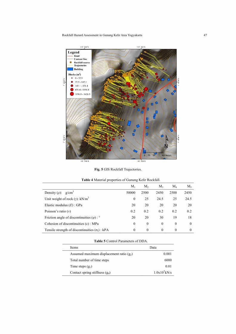
The rockfall trajectory shows that the northern part and middle part have higher susceptibility

than the southern part (Fig. 5). There are three buildings potentially obstructed by rockfall. The

location of the building is 163 meters from the source of material. The result of the rockfall

trajectory model shows that no one of the building is obstructed by rockfall in the southern part.

The size of the boulder deposition in the southern part is also relatively small < 20 m3.

More attention should be prioritized in northern and middle part that can potentially cause

building damage. However, the detail of preventive measures development needs more analysis on

the mechanic of rockfall process. Thus, 2D DDA was applied to explore the motion behavior of

rockfall in the highest potency of high risk. There are 5 materials involved to model the motion

behavior of a boulder which has the potential to damage the building in the northern part. The

material properties are shown in Table 4 and control parameter is shown in Table 5.


Fig. 5 GIS Rockfall Trajectories.

Table 4 Material properties of Gunung Kelir Rockfall.

M1 M2 M3 M4 M5

Density (ρ): g/cm3 50000 2500 2450 2500 2450

Unit weight of rock (γ): kN/m3 0 25 24.5 25 24.5

Elastic modulus (E) : GPa 20 20 20 20 20

Poisson’s ratio (v) 0.2 0.2 0.2 0.2 0.2

Friction angle of discontinuities (φ) : ° 20 20 30 19 18

Cohesion of discontinuities (c) : MPa 0 0 0 0 0

Tensile strength of discontinuities (σt) : kPA 0 0 0 0 0

Table 5 Control Parameters of DDA.

Items Data

Assumed maximum displacement ratio (g2) 0.001

Total number of time steps 6000

Time steps (g1) 0.01

Contact spring stiffness (g0) 1.0x107kN/s


Fig. 6 Rockfall Impact Force.

The result shows that the boulder in the northern part can potentially cause the building damage.

The contact between boulder and building was introduced by small boulders with impact force 0.4

MPa at 30.95 seconds. The maximum impact force between boulders and building was 11.9 MPa

(32.74 seconds after failure) (Fig. 6 and Fig. 7). It happened before the contact between the big

boulder and the building. It was almost 80 times higher compared with the first contact between

small boulders and the building. After the maximum impact force, it was followed by contact

between medium boulder and the building with the maximum impact force 2.3 MPa in 33.4

seconds. Then, finally the small boulders stoped moving in 43.04 seconds with the impact force

around 0.91. The velocity of the boulders is less than 15 m/s. Rolling and sliding are the most

common of boulders motion.

Fig. 7 Rockfall Behaviour for Potential High Risk.

By defining spatial, temporal and intensity distribution of rockfall; structural protection, land

planning and or evacuation can be designed effectively. Information of trajectories and deposition

is useful for landuse planning. Landuse planning is related to area zoning which needs rockfall

information including spatial probability of rockfall hazard, trajectories and final deposition

information. Rockfall information can assist policy maker to make zonation on high risk and

acceptable risk zone.

0

2

4

6

8

10

12

14

0 10 20 30 40 50 60

Impa

ct (

MP

a)

Time (Seconds)


In the case of Gunung Kelir area, it is also possible to establish structural preventive measures

along the escarpment. However, it is difficult to install structural preventive measures along the

escarpment due to limitation of the budget and the socioeconomic condition of Gunung Kelir Area.

Thus, the information of trajectories, velocity, impact, and final deposition can assist policy maker

to make prioritization for protecting important assets by establishing several scenarios of

preventive measures and computing a cost-benefit ratio of applied mitigation technique.

5 Conclusion

Hazard assessment as defined by spatial, temporal and intensity distribution should involve

determination of rockfall source, size-frequency, onset susceptibility, temporal probability and

deposit area. It represents "where", “how frequent” and “how large” rockfall are likely to occur.

GIS-lumped mass rockfall simulation has been employed to identify potential rockfall source based

on the distribution of boulders from the past rockfall events. The reliable trajectories can be

estimated once the potential rockfall sources were identified. It represents where rockfall is likely

to occur called as susceptibility. The rockfall susceptibility shows that the northern part and middle

part have higher susceptibility than the southern part and may cause three building damage

obstructed by rockfall (potential high risk). More attention should be prioritized on the potential

high risk. Since GIS-lumped mass model does not consider the size, shape and fragmentation of the

boulder, the more mechanically numerical rockfall simulation is needed as a complementary tool to

analyze the trajectory which has a potency of high risk. Thus, 2D DDA was employed to confirm

the reliable trajectory and dynamic behavior of boulder when travel along the slope having high

risk possibility. Thus, the methodological framework resulting information of rockfall hazard

represented as the susceptible location and magnitude-frequency, including temporal probability of

rockfall can be further employed to formulate an appropriate landuse plan in a rockfall prone area.

Acknowledgements

The authors would like to acknowledge the funding of Hibah Bersaing DIKTI research grant

(contract number UGM/PHB/XVI/2010/1) for field work and data collection.

References

1) O. Hungr and S. G. Evans. Engineering evaluation of fragmental rockfall hazards,

Proceedings 5th International Symposium on Landslides, Lausanne, Switzerland, 1, 685–690,

(1988).

2) C. Dussauge, J. Grasso, and A. Helmstetter. Statistical analysis of rockfall volume

distributions: Implications for rockfall dynamics. Journal of Geophysical Research 108

(2003).

3) G. B. Crosta and F.Agliardi. A methodology for physically based rockfall hazard assessment,

Nat. Hazards Earth Syst. Sci., 3,407–422 (2003).

4) D. Peila, C. Oggeri, C. Castiglia. Ground reinforced embankments for rockfall protection:

design and evaluation of full scale tests, Landslides 4 : 255-265 (2007).

5) A. Loye, M. Jaboyedoff, A. Pedrazzini. Identification of Potential Rockfall Source areas at

regional scale using DEM-based geomorphometric analysis, Nat. Hazards Earth Syst. Sci.,

9,1643–1653 (2009).

6) M. Jaboyedoff, and V.Labiouse. Preliminary assessment of rockfall hazard based on GIS data,

in: 10th International Congress on Rock Mechanics ISRM 2003 – Technology roadmap for


rock mechanics, South African Institute of Mining and Metallurgy, Johannesburgh, South

Africa, 575–578 (2003).

7) F. Guzzetti, P. Reichenbach, and G. F. Wieczorek. Rockfall hazard and risk assessment in the

Yosemite Valley, California, USA,Nat. Hazards Earth Syst. Sci., 3, 491–503 (2003).

8) P. Frattini, G. Crosta, A. Carrara, and F. Agliardi. Assessment of rockfall susceptibility by

integrating statistical and physicallybased approaches, Geomorphology, 94, 419–437 (2008).

9) H. Aksoy, and M. Ercanoglu. Determination of the rockfall source in an urban settlement area

by using a rule-based fuzzy evaluation, Nat. Hazards Earth Syst. Sci., 6, 941–954 (2006).

10) H. Lan, C.D. Martin, C. Zhou, C.H. Lim. Rockfall hazard analysis using LiDAR and spatial

modeling. Geomorphology 118 (1–2), 213–223 (2010).

11) D. Santana, J. Corominas, O. Mavrouli, D. Garcia-Selles. Magnitude-frequency relation for

rockfall scars using a Terrestrial Laser Scanner. Engineering Geology 145-146 50-64 (2012).

12) G. F. Wieczorek, J. B. Snyder, C. S. Alger, and K. A. Isaacson, Yosemite historical rockfall

inventory, U.S Geol. Surv. Open File Rep., 92– 387, 38 pp. (1992).

13) O. Hungr, S. G. Evans, and J. Hazzard, Magnitude and frequency of rock falls along the main

transportation corridors of southwestern British Columbia, Can. Geotech. J., 36, 224–238.

(1999).

14) C. Dussauge-Peisser, A. Helmstetter, J. R. Grasso, D. Hantz, P. Desvarreux, M. Jeannin, and

A. Giraud. Probabilistic approach to rock fall hazard assessment: potential of historical data

analysis, Nat. Hazards Earth Syst. Sci. 2, 15–26 (2002).

15) A. Volkwein, K. Schellenberg, V. Labiouse, F. Agliardi, F. Berger, F. Bourrier, L. K. A.

Dorren, W. Gerber, M. Jaboyedoff. Rockfall characterisation and structural protection—a

review. Nat Hazards Earth Syst 11:2617–2651 (2011).

16) F. Guzzetti, G. Crosta, R. Detti, F. Agliardi. STONE: a computer program for

three-dimensional simulation of rock-falls. Computer & Geosciences 28 pp. 1079-1093

(2002).

17) G. Shi. Discontinuous deformation analysis a new numerical model for the static and

dynamics of block systems. Ph. D thesis. Berkeley University of California (1988).

18) Winaryo and Sunarto Pengkajian Mitigasi Tanah Longsor Pasca Gempabumi 27 Mei 2006 di

Dusun Gunung Kelir, Kecamatan Girimulyo, Kabupaten Kulon Progo DIY. Jurnal

Kebencanaan Indonesia (2008).

19) PSBA UGM. Penyusunan Sistem Informasi Penanggulangan Bencana Tanah Longsor di

Kabupaten Kulon Progo. UGM (2008).

20) R.W. van Bemmelen. The Geology of Indonesia, Vol II., GovernmentPrinting Office the

Hague (1949).

21) M. Cardinali, F. Guzzetti, E.E. Brabb. Preliminary map showing landslide deposits and

related features in New Mexico. U.S. Geological Survey Open File Report 90/293, 4 sheets,

scale 1:500,000 (1990).

22) F. Brardinoni, O. Slaymaker, M.A. Hassan. Landslide inventory in a rugged forested

watershed: a comparison between air-photo and field survey data. Geomorphology 54 (3–4),

179–196 (2003).

23) T.Y. Duman, T. Çan, Ö. Emre, M. Keçer, A. Doğan, A. Şerafettin, D. Serap. Landslide

inventory of northwestern Anatolia, Turkey. Engineering Geology 77(1–2), 99–114 (2005).

24) F. Fiorucci, M. Cardinali, R. Carlà, M. Rossi, A.C. Mondini, L. Santurri, F. Ardizzone, F.

Guzzetti. Seasonal landslides mapping and estimation of landslide mobilization rates using

aerial and satellite images. Geomorphology 129 (1–2), 59–70 (2011).


25) W.H. Schulz. Landslides Mapped using LIDAR Imagery, Seattle, Washington. U.S.

Geological Survey Open-File Report 2004-1396 (2004).

26) M.H. Derron and M. Jaboyedoff. Preface to the special issue: LIDAR and DEM techniques

for landslides monitoring and characterization. Natural Hazards and Earth System Sciences 10

(9), 1877–1879 (2010).

27) K.A. Razak, M.W. Straatsma, C.J. van Westen, J.-P. Malet, S.M. de Jong.. Airborne laser

scanning of forested landslides characterization: terrain model quality and visualization.

Geomorphology 126, 186–200. (2011).

28) J. Barlow, S. Franklin, Y. Martin. High spatial resolution satellite imagery, DEM derivatives,

and image segmentation for the detection of mass wasting processes. Photogrammetric

Engineering and Remote Sensing 72, 687–692 (2006).

29) A.M. Borghuis, K. Chang, H.Y. Lee. Comparison between automated and manual mapping of

typhoon-triggered landslides from SPOT-5 imagery. International Journal of Remote Sensing

28, 1843–1856 (2007).

30) Z. Ren and A. Lin. Co-seismic landslides induced by the Wenchuan Mw 7.9 earthquake,

revealed by ALOS PRISM and AVNIR2 imagery data. International Journal of Remote

Sensing 31, 3479–3493 (2010).

31) J. R.Taylor. An Introduction to Error Analysis, 2nd Ed., 327 pp., Univ. Sci. Books, Sausalito,

Calif. (1997).

32) H. Lan, C. D. Martin, and C. H. Lim. RockFall analyst: a GIS extension for three-dimensional

and spatially distributed rockfall hazard modelling, Computer and Geoscience., 33, 262–279

(2007).

33) G. Chen. Numerical Modelling of Rockfall using Extended DDA. Chinese Journal of Rock

Mechanics and Engineering, 22 (6):926-931 (2003).

34) G. Shi and R. E. Goodman. Generalization of Two-Dimensional Discontinuous Deformation

Analysis for Forward Modelling. International Journal for Numerical and Analytical Methods

in Geomechanics, vol. 13, pp. 359-380 (1989).

35) G. Shi and R. E. Goodman. Two dimensional Discontinuous Deformation Analysis.

International Journal for Numerical and Analytical Methods in Geomechanics, vol. 9, pp.

541-556 (1985).

36) Joint Technical Committee on Landslide and Engineered Slope (JTC-1). Guidelines for

Landslide Susceptibility, Hazard and Risk Zoning for Landuse Planning. Engineering

Geology 103, 85-98 (2008).

Rockfall Hazard Assessment in Gunung Kelir Area Yogyakarta...

Documents

Transcript of Rockfall Hazard Assessment in Gunung Kelir Area Yogyakarta...