PRELIMINARY REGIONAL ROCKFALL HAZARD MAPPING USING LIDAR-BASED SLOPE FREQUENCY DISTRIBUTION AND CONEFALL MODELLING Alexandre Loye Institute of Geomatics and Risk Analysis, University of Lausanne, Switzerland, alexandre.loye@unil.ch Andrea Pedrazzini and Michel Jaboyedoff Institute of Geomatics and Risk Analysis, University of Lausanne, Switzerland RÉSUMÉ L’élaboration des cartes de danger à l’échelle régionale est souvent limitée par le manque de connaissance des zones sources potentielles. Grâce aux données numériques de terrain haute-résolutions (LiDAR), l’analyse morphométrique de la topographie est devenue une approche appropriée pour détecter les instabilités rocheuses sur des surfaces relativement étendues. A l’aide du concept des « familles de pentes » tiré du modèle numérique de terrain (MNT) laser et autres documents contenu dans la carte topographique nationale, une carte des dangers potentiels chute du bloc a été établie sur l’ensemble du canton de Vaud, Suisse. Les zones sources potentielles sont définies à partir de seuils de pentes établis par analyse géomorphométrique et leur propagation maximale modélisée à l’aide du logiciel CONEFALL. Une comparaison avec les données de terrain ainsi qu’un modèle trajectographique révèle de grandes concordances, démontrant qu’il est possible d’évaluer le danger chute de bloc à grande échelle à partir de paramètres extraits du MNT et des éléments topographiques. ABSTRACT A factor limiting preliminary rockfall hazard mapping at regional scale is often the lack of knowledge of potential source areas. Nowadays, high resolution topographic data (LiDAR) can account for realistic landscape details even at large scale. With such fine-scale morphological variability, quantitative geomorphometric analyses become a relevant approach for delineating potential rockfall instabilities. Using digital elevation model (DEM)-based “slope families” concept over areas of similar lithology and cliffs and screes zones available from the 1:25,000 topographic map, a susceptibility rockfall hazard map was drawn up in the canton of Vaud, Switzerland, in order to provide a relevant hazard overview. Slope surfaces over morphometrically-defined thresholds angles were considered as rockfall source zones. 3D modelling (CONEFALL) was then applied on each of the estimated source zones in order to assess the maximum runout length. Comparison with known events and other rockfall hazard assessments are in good agreement, showing that it is possible to assess rockfall activities over large areas from DEM-based parameters and topographical elements. 1. INTRODUCTION To assess whether an area is potentially endangered by rockfall, preliminary hazard mapping throughout relatively large mountainous zones provides a fast and cost-effective overview of rockfall prone areas. In the framework of susceptibility mapping, the purpose consists of defining potentially rockfall sources zones and their runout zones for rockfall of small size (Lateltin, 1997). Larger events, such as rock avalanches, cannot be taken into account in this modelling approach, because the runout distance depends on the sliding volume (Scheidegger, 1973). The outcome gives a susceptibility hazard map, which can be used as a scientific reference for regional policies of territory management. The increasing availability of geographic information system (GIS) data, such as digital elevation models (DEM) and topographic vector maps, makes GIS-based and 3D modelling approach very convenient to predict hazards posed by rockfall at regional scales. One of the great limiting factors, however, in predicting and therefore mapping rockfall prone areas, is the lack of knowledge of the potential rockfall source areas and fall tracks. Rockfall sources areas are usually taken from distinctive evidence, such as talus slope deposits at the foot of steep cliff faces or as information extracted from maps (historical register of

observations, field measurements) (Hantz, 2003). But rockfalls also occur on slope surfaces covered with vegetation where evidence is less distinct and their related sources areas are not taken into account in planning rockfall hazard assessment. A variety of empirical and process-based rockfall models exist (Dorren, 2003), but were developed for specifically known regions where rockfall causes problems. Only a few methods were tested for predicting rockfall runout zones at a regional scale (>500km2) (Dorren et al, 2000; Crosta et al, 2003). For a preliminary assessment of the runout length, the integration of empirical or process-based methods in GIS has shown very promising results (ie, Meissl, 1998; Van Dijke & Van Westen, 1990; Jaboyedoff & Labiouse, 2003). Those models can be defined as distributed models, since they are process-based and they take into account the spatial variability within a certain region. Terrain properties are represented by multiple rasters derived from GIS data layers (Dorren, 2003). Identification of rockfall source areas has started with simple methods that consist of defining thresholds for mean slope gradients (Toppe, 1987; Van Dijke & Van Westen, 1990) or for steep slopes (e.g. > 45°; Jaboyedoff & Labiouse, 2003). Rockfall source areas have also been derived from cliff faces and rocky outcrops on topographical maps (Krummenacher, 1995; Meissl, 1998) or from areas defined as active rockfall slopes on

In : J. Locat, D. Perret, D. Turmel, D. Demers et S. Leroueil, (2008). Comptes rendus de la 4e Conférence canadienne sur les géorisques: des causes à la gestion. Proceedings of the 4th Canadian Conference on Geohazards : From Causes to Management. Presse de l’Université Laval, Québec, 594 p.

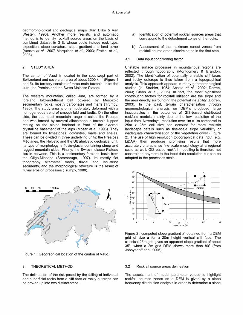
geomorphological and geological maps (Van Dijke & Van Westen, 1990). Another more realistic and automatic method is to identify rockfall source areas on the basis of combined dataset in GIS, whose could include rock type, exposition, slope curvature, slope gradient and land cover (Acosta et al., 2007 Marquinez et al., 2003; Frattini et al., 2008). 2. STUDY AREA The canton of Vaud is located in the southwest part of Switzerland and covers an area of about 3200 km2 (Figure 1 and 5). Its territory consists of three main tectonic units: the Jura, the Prealps and the Swiss Molasse Plateau. The western mountains, called Jura, are formed by a foreland fold-and-thrust belt covered by Mesozoic sedimentary rocks, mostly carbonates and marls (Trümpy, 1980). The study area is only moderately deformed with a homogeneous trend of smooth fold and faults. On the other side, the southeast mountain range is called the Prealps and was formed by several allochthonous tectonic klippen resting on the alpine foreland in front of the external crystalline basement of the Alps (Mosar et al. 1996). They are formed by limestones, dolomites, marls and shales. These can be divided in three underlying units: the Préalpes Médianes, the Helvetic and the Ultrahelvetic geological unit. Its type of morphology is fluvio-glacial containing steep and rugged mountain sides. Finally, the Swiss molasse Plateau lies in between. This is a sedimentary foreland basin from the Oligo-Miocene (Sommaruga, 1997). Its mostly flat topography alternates marin, fluvial and lacustrine sediments, and the morphological structure is the result of fluvial erosion processes (Trümpy, 1980).

Figure 1 : Geographical location of the canton of Vaud. 3. THEORETICAL METHOD The delineation of the risk posed by the falling of individual and superficial rocks from a cliff face or rocky outcrops can be broken up into two distinct steps:

a) Identification of potential rockfall sources areas that

correspond to the detachment zones of the rocks. b) Assessment of the maximum runout zones from

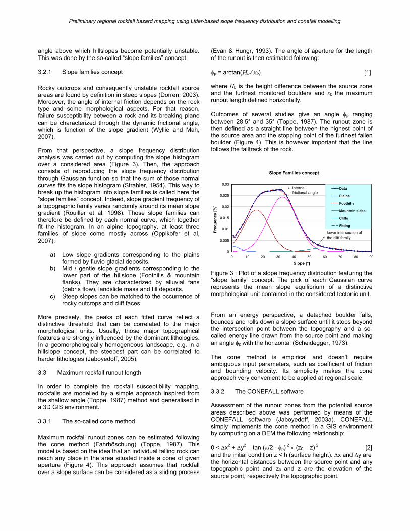
rockfall source areas discriminated in the first step. 3.1 Data input conditioning factor Unstable surface processes in mountainous regions are reflected through topography (Montgomery & Brandon, 2002). The identification of potentially unstable cliff faces and rocky outcrops is thus taken from a topographical analysis. This approach appears in many geomorphological studies (ie. Strahler, 1954; Acosta et al., 2002; Dorren, 2003; Glenn et al., 2005). In fact, the most significant contributing factors for rockfall initiation are the slope and the area directly surrounding the potential instability (Dorren, 2003). In the past, terrain characterisation through geomorphological analysis on DEM’s produced large inaccuracies in the outcomes of GIS-based distributed rockfalls models, mainly due to the low resolution of the input data. Nowadays, resolution over 1m x 1m compared to 25m x 25m cell size can account for more realistic landscape details such as fine-scale slope variability or inadequate characterisation of the vegetation cover (Figure 2). The use of high resolution topographical data input (e.g. LiDAR) then produces promising results that more accurately characterise fine-scale morphology at a regional scale as well. GIS-based rockfall modelling is therefore not constrained anymore to the input data resolution but can be adapted to the processes scale.

Figure 2 : computed slope gradient α° obtained from a DEM grid of size a for a 20m height vertical cliff face. The classical 25m grid gives an apparent slope gradient of about 35°, when a 2m grid DEM shows more than 80° (from Jaboyedoff et al. 2005). 3.2 Rockfall source areas delineation The assessment of model parameter values to highlight rockfall sources zones on a DEM is given by a slope frequency distribution analysis in order to determine a slope

A. Loye et al.

angle above which hillslopes become potentially unstable. This was done by the so-called “slope families” concept. 3.2.1 Slope families concept Rocky outcrops and consequently unstable rockfall source areas are found by definition in steep slopes (Dorren, 2003). Moreover, the angle of internal friction depends on the rock type and some morphological aspects. For that reason, failure susceptibility between a rock and its breaking plane can be characterized through the dynamic frictional angle, which is function of the slope gradient (Wyllie and Mah, 2007). From that perspective, a slope frequency distribution analysis was carried out by computing the slope histogram over a considered area (Figure 3). Then, the approach consists of reproducing the slope frequency distribution through Gaussian function so that the sum of those normal curves fits the slope histogram (Strahler, 1954). This way to break up the histogram into slope families is called here the “slope families” concept. Indeed, slope gradient frequency of a topographic family varies randomly around its mean slope gradient (Rouiller et al, 1998). Those slope families can therefore be defined by each normal curve, which together fit the histogram. In an alpine topography, at least three families of slope come mostly across (Oppikofer et al, 2007):

a) Low slope gradients corresponding to the plains formed by fluvio-glacial deposits.

b) Mid / gentle slope gradients corresponding to the lower part of the hillslope (Foothills & mountain flanks). They are characterized by alluvial fans (debris flow), landslide mass and till deposits.

c) Steep slopes can be matched to the occurrence of rocky outcrops and cliff faces.

More precisely, the peaks of each fitted curve reflect a distinctive threshold that can be correlated to the major morphological units. Usually, those major topographical features are strongly influenced by the dominant lithologies. In a geomorphologically homogeneous landscape, e.g. in a hillslope concept, the steepest part can be correlated to harder lithologies (Jaboyedoff, 2005). 3.3 Maximum rockfall runout length In order to complete the rockfall susceptibility mapping, rockfalls are modelled by a simple approach inspired from the shallow angle (Toppe, 1987) method and generalised in a 3D GIS environment. 3.3.1 The so-called cone method Maximum rockfall runout zones can be estimated following the cone method (Fahrböschung) (Toppe, 1987). This model is based on the idea that an individual falling rock can reach any place in the area situated inside a cone of given aperture (Figure 4). This approach assumes that rockfall over a slope surface can be considered as a sliding process

(Evan & Hungr, 1993). The angle of aperture for the length of the runout is then estimated following: φp = arctan(Hb/xb) [1] where Hb is the height difference between the source zone and the furthest monitored boulders and xb the maximum runout length defined horizontally. Outcomes of several studies give an angle φp ranging between 28.5° and 35° (Toppe, 1987). The runout zone is then defined as a straight line between the highest point of the source area and the stopping point of the furthest fallen boulder (Figure 4). This is however important that the line follows the falltrack of the rock.

Slope Families concept

0

0.005

0.01

0.015

0.02

0.025

0.03

0 10 20 30 40 50 60 70 80 90

Slope [°]

Freq

uenc

y [%

]

Data

Plains

Foothills

Mountain sides

Cliffs

Fitting

internalfrictional angle

lower intersection ofthe cliff family

Figure 3 : Plot of a slope frequency distribution featuring the “slope family” concept. The pick of each Gaussian curve represents the mean slope equilibrium of a distinctive morphological unit contained in the considered tectonic unit. From an energy perspective, a detached boulder falls, bounces and rolls down a slope surface until it stops beyond the intersection point between the topography and a so-called energy line drawn from the source point and making an angle φp with the horizontal (Scheidegger, 1973). The cone method is empirical and doesn’t require ambiguous input parameters, such as coefficient of friction and bounding velocity. Its simplicity makes the cone approach very convenient to be applied at regional scale. 3.3.2 The CONEFALL software Assessment of the runout zones from the potential source areas described above was performed by means of the CONEFALL software (Jaboyedoff, 2003a). CONEFALL simply implements the cone method in a GIS environment by computing on a DEM the following relationship: 0 < Δx2 + Δy2 – tan (π/2 - φp) 2 × (z0 – z) 2 [2] and the initial condition z < h (surface height). Δx and Δy are the horizontal distances between the source point and any topographic point and z0 and z are the elevation of the source point, respectively the topographic point.

Preliminary regional rockfall hazard mapping using Lidar-based slope frequency distribution and conefall modelling

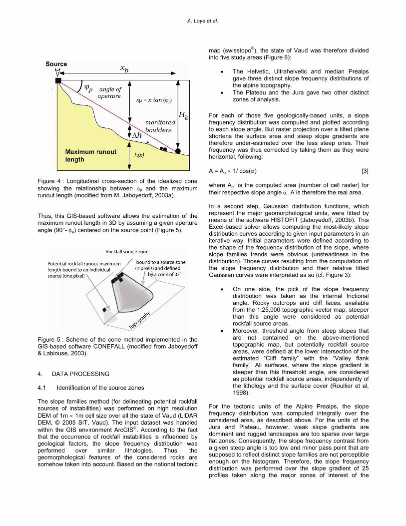
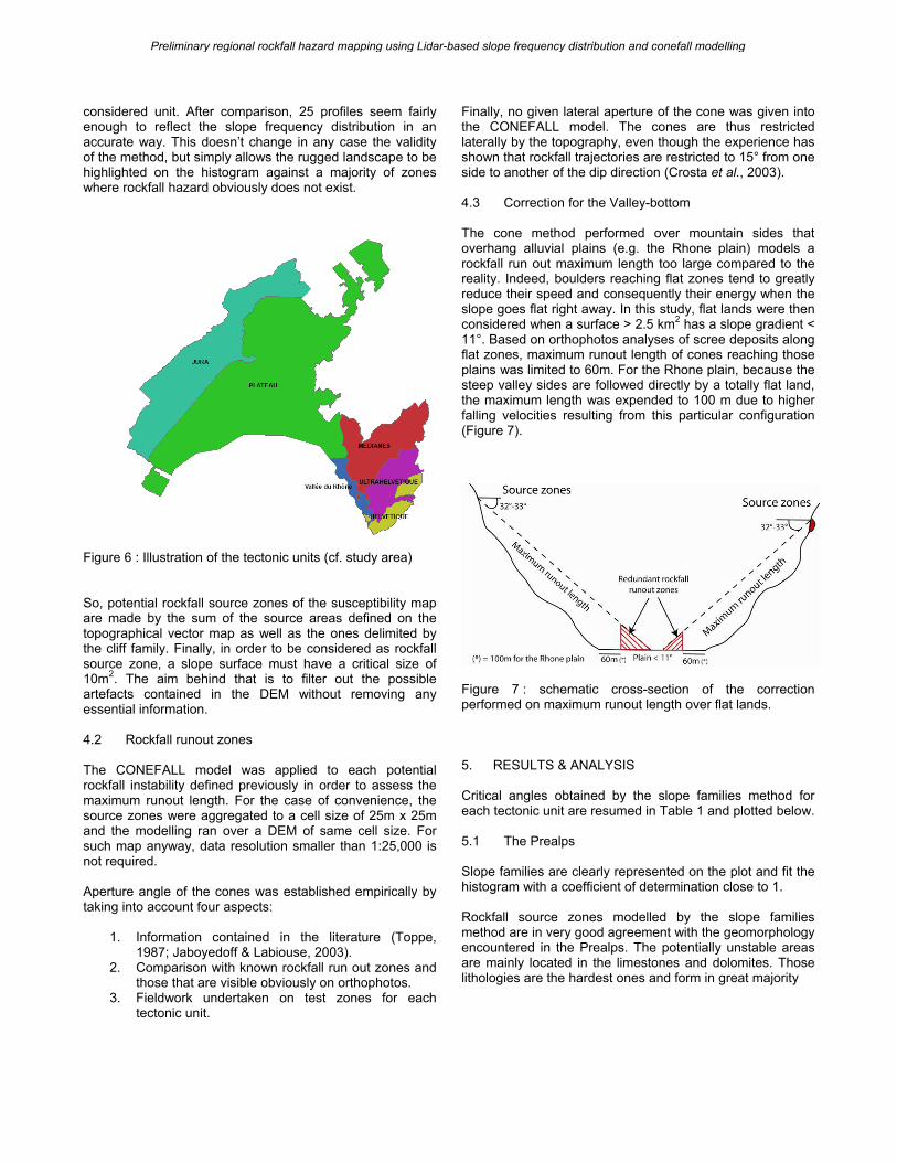
Figure 4 : Longitudinal cross-section of the idealized cone showing the relationship between φp and the maximum runout length (modified from M. Jaboyedoff, 2003a). Thus, this GIS-based software allows the estimation of the maximum runout length in 3D by assuming a given aperture angle (90°- φp) centered on the source point (Figure 5).

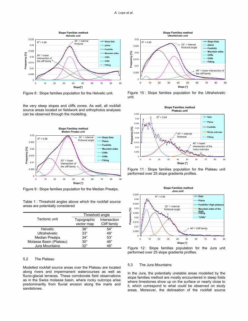
Figure 5 : Scheme of the cone method implemented in the GIS-based software CONEFALL (modified from Jaboyedoff & Labiouse, 2003). 4. DATA PROCESSING 4.1 Identification of the source zones The slope families method (for delineating potential rockfall sources of instabilities) was performed on high resolution DEM of 1m × 1m cell size over all the state of Vaud (LIDAR DEM, © 2005 SIT, Vaud). The input dataset was handled within the GIS environment ArcGIS®. According to the fact that the occurrence of rockfall instabilities is influenced by geological factors, the slope frequency distribution was performed over similar lithologies. Thus, the geomorphological features of the considered rocks are somehow taken into account. Based on the national tectonic

map (swisstopo©), the state of Vaud was therefore divided into five study areas (Figure 6):

• The Helvetic, Ultrahelvetic and median Prealps gave three distinct slope frequency distributions of the alpine topography.

• The Plateau and the Jura gave two other distinct zones of analysis.

For each of those five geologically-based units, a slope frequency distribution was computed and plotted according to each slope angle. But raster projection over a tilted plane shortens the surface area and steep slope gradients are therefore under-estimated over the less steep ones. Their frequency was thus corrected by taking them as they were horizontal, following: A = Aα × 1/ cos(α) [3] where Aα is the computed area (number of cell raster) for their respective slope angle α. A is therefore the real area. In a second step, Gaussian distribution functions, which represent the major geomorphological units, were fitted by means of the software HISTOFIT (Jaboyedoff, 2003b). This Excel-based solver allows computing the most-likely slope distribution curves according to given input parameters in an iterative way. Initial parameters were defined according to the shape of the frequency distribution of the slope, where slope families trends were obvious (unsteadiness in the distribution). Those curves resulting from the computation of the slope frequency distribution and their relative fitted Gaussian curves were interpreted as so (cf. Figure 3):

• On one side, the pick of the slope frequency distribution was taken as the internal frictional angle. Rocky outcrops and cliff faces, available from the 1:25,000 topographic vector map, steeper than this angle were considered as potential rockfall source areas.

• Moreover, threshold angle from steep slopes that are not contained on the above-mentioned topographic map, but potentially rockfall source areas, were defined at the lower intersection of the estimated “Cliff family” with the “Valley flank family”. All surfaces, where the slope gradient is steeper than this threshold angle, are considered as potential rockfall source areas, independently of the lithology and the surface cover (Roullier et al, 1998).

For the tectonic units of the Alpine Prealps, the slope frequency distribution was computed integrally over the considered area, as described above. For the units of the Jura and Plateau, however, weak slope gradients are dominant and rugged landscapes are too sparse over large flat zones. Consequently, the slope frequency contrast from a given steep angle is too low and minor pass point that are supposed to reflect distinct slope families are not perceptible enough on the histogram. Therefore, the slope frequency distribution was performed over the slope gradient of 25 profiles taken along the major zones of interest of the

A. Loye et al.

considered unit. After comparison, 25 profiles seem fairly enough to reflect the slope frequency distribution in an accurate way. This doesn’t change in any case the validity of the method, but simply allows the rugged landscape to be highlighted on the histogram against a majority of zones where rockfall hazard obviously does not exist.

Figure 6 : Illustration of the tectonic units (cf. study area) So, potential rockfall source zones of the susceptibility map are made by the sum of the source areas defined on the topographical vector map as well as the ones delimited by the cliff family. Finally, in order to be considered as rockfall source zone, a slope surface must have a critical size of 10m2. The aim behind that is to filter out the possible artefacts contained in the DEM without removing any essential information. 4.2 Rockfall runout zones The CONEFALL model was applied to each potential rockfall instability defined previously in order to assess the maximum runout length. For the case of convenience, the source zones were aggregated to a cell size of 25m x 25m and the modelling ran over a DEM of same cell size. For such map anyway, data resolution smaller than 1:25,000 is not required. Aperture angle of the cones was established empirically by taking into account four aspects:

1. Information contained in the literature (Toppe, 1987; Jaboyedoff & Labiouse, 2003).

2. Comparison with known rockfall run out zones and those that are visible obviously on orthophotos.

3. Fieldwork undertaken on test zones for each tectonic unit.

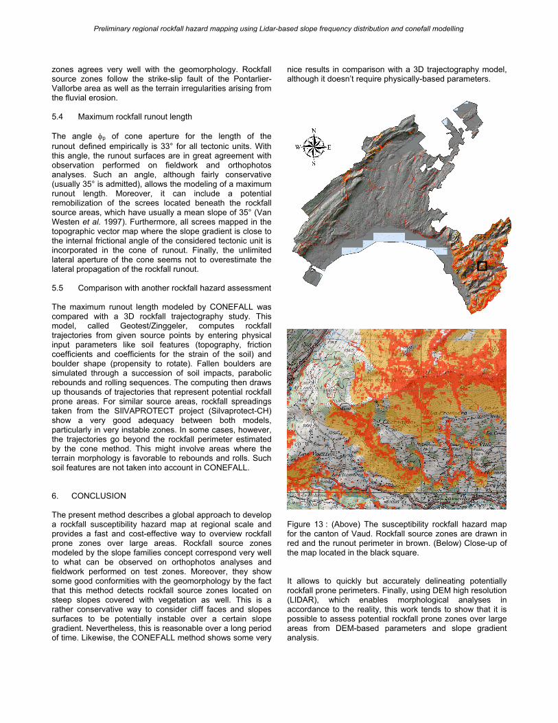
Finally, no given lateral aperture of the cone was given into the CONEFALL model. The cones are thus restricted laterally by the topography, even though the experience has shown that rockfall trajectories are restricted to 15° from one side to another of the dip direction (Crosta et al., 2003). 4.3 Correction for the Valley-bottom The cone method performed over mountain sides that overhang alluvial plains (e.g. the Rhone plain) models a rockfall run out maximum length too large compared to the reality. Indeed, boulders reaching flat zones tend to greatly reduce their speed and consequently their energy when the slope goes flat right away. In this study, flat lands were then considered when a surface > 2.5 km2 has a slope gradient < 11°. Based on orthophotos analyses of scree deposits along flat zones, maximum runout length of cones reaching those plains was limited to 60m. For the Rhone plain, because the steep valley sides are followed directly by a totally flat land, the maximum length was expended to 100 m due to higher falling velocities resulting from this particular configuration (Figure 7).

Figure 7 : schematic cross-section of the correction performed on maximum runout length over flat lands. 5. RESULTS & ANALYSIS Critical angles obtained by the slope families method for each tectonic unit are resumed in Table 1 and plotted below. 5.1 The Prealps Slope families are clearly represented on the plot and fit the histogram with a coefficient of determination close to 1. Rockfall source zones modelled by the slope families method are in very good agreement with the geomorphology encountered in the Prealps. The potentially unstable areas are mainly located in the limestones and dolomites. Those lithologies are the hardest ones and form in great majority

Preliminary regional rockfall hazard mapping using Lidar-based slope frequency distribution and conefall modelling

Slope Families methodHelvetic unit

0

0.005

0.01

0.015

0.02

0.025

0.03

0.035

0 10 20 30 40 50 60 70 80 90

Slope[°]

Freq

uenc

y [%

]

Slope Data

plains

Foothills

Mountain sides

Cliffs

Cliffs

Fitting

36° = internal frictional

l

54° = lower intersection ofthe cliff family

R2 = 0.98

Figure 8 : Slope families population for the Helvetic unit. the very steep slopes and cliffs zones. As well, all rockfall source areas located on fieldwork and orthophotos analyses can be observed through the modelling.

Slope Families methodMedian Prealps unit

0

0.005

0.01

0.015

0.02

0.025

0.03

0 10 20 30 40 50 60 70 80 90

Slope [°]

Freq

uenc

y [%

]

Slope Data

Plains

Foothills

Mountain sides

Cliffs

Cliffs

Fitting

34° = internal frictional angle

53° = lower intersection ofthe cliff family

R2 = 0.98

Figure 9 : Slope families population for the Median Prealps. Table 1 : Threshold angles above which the rockfall source areas are potentially considered

Threshold angle Tectonic unit Topographic

vector map Intersection Cliff family

Helvetic 36° 54° Ultrahelvetic 33° 49°

Median Prealps 34° 53° Molasse Basin (Plateau) 30° 46°

Jura Mountains 32° 46° 5.2 The Plateau Modelled rockfall source areas over the Plateau are located along rivers and impermanent watercourses as well as fluvio-glacial terraces. These corroborate field observations as in the Swiss molasse basin, where rocky outcrops arise predominantly from fluvial erosion along the marls and sandstones.

Slope Families methodUltraHelvetic unit

0

0.005

0.01

0.015

0.02

0.025

0.03

0 10 20 30 40 50 60 70 80 90

Slope [°]

Freq

uenc

y [%

]

Slope DataplainsFoothillsMountain sidesCliffsCliffsFitting

33° = internal frictional angle

49° = lower intersection ofthe cliff family

R2 = 0.99

Figure 10 : Slope families population for the Ultrahelvetic unit.

Slope Families methodPlateau unit

0

0.005

0.01

0.015

0.02

0.025

0.03

0.035

0.04

0.045

0 10 20 30 40 50 60 70 80 90

Slope [°]

Freq

uenc

y [%

]

Data

Plains

Foothills

Rocky outcrops

Fitting

46° = lower intersection of the rocky outcrops f

R2 = 0.94

30° = internal frictional

Figure 11 : Slope families population for the Plateau unit performed over 25 slope gradients profiles.

Slope Families methodJura unit

0

0.005

0.01

0.015

0.02

0.025

0.03

0.035

0.04

0.045

0 10 20 30 40 50 60 70 80 90

Slope [°]

Freq

uenc

y [%

]

Data

Plains

Foothills+ High plateaus

Mountain sides of thefoldsFitting

"Cliffs"

32° = internal frictional angle

46°= Cliff family

R2 = 0.96

Figure 12 : Slope families population for the Jura unit performed over 25 slope gradients profiles. 5.3 The Jura Mountains In the Jura, the potentially unstable areas modelled by the slope families method are mostly encountered in steep folds where limestones show up on the surface or nearly close to it, which correspond to what could be observed on study areas. Moreover, the delineation of the rockfall source

A. Loye et al.

zones agrees very well with the geomorphology. Rockfall source zones follow the strike-slip fault of the Pontarlier-Vallorbe area as well as the terrain irregularities arising from the fluvial erosion. 5.4 Maximum rockfall runout length The angle φp of cone aperture for the length of the runout defined empirically is 33° for all tectonic units. With this angle, the runout surfaces are in great agreement with observation performed on fieldwork and orthophotos analyses. Such an angle, although fairly conservative (usually 35° is admitted), allows the modeling of a maximum runout length. Moreover, it can include a potential remobilization of the screes located beneath the rockfall source areas, which have usually a mean slope of 35° (Van Westen et al. 1997). Furthermore, all screes mapped in the topographic vector map where the slope gradient is close to the internal frictional angle of the considered tectonic unit is incorporated in the cone of runout. Finally, the unlimited lateral aperture of the cone seems not to overestimate the lateral propagation of the rockfall runout. 5.5 Comparison with another rockfall hazard assessment The maximum runout length modeled by CONEFALL was compared with a 3D rockfall trajectography study. This model, called Geotest/Zinggeler, computes rockfall trajectories from given source points by entering physical input parameters like soil features (topography, friction coefficients and coefficients for the strain of the soil) and boulder shape (propensity to rotate). Fallen boulders are simulated through a succession of soil impacts, parabolic rebounds and rolling sequences. The computing then draws up thousands of trajectories that represent potential rockfall prone areas. For similar source areas, rockfall spreadings taken from the SIlVAPROTECT project (Silvaprotect-CH) show a very good adequacy between both models, particularly in very instable zones. In some cases, however, the trajectories go beyond the rockfall perimeter estimated by the cone method. This might involve areas where the terrain morphology is favorable to rebounds and rolls. Such soil features are not taken into account in CONEFALL. 6. CONCLUSION The present method describes a global approach to develop a rockfall susceptibility hazard map at regional scale and provides a fast and cost-effective way to overview rockfall prone zones over large areas. Rockfall source zones modeled by the slope families concept correspond very well to what can be observed on orthophotos analyses and fieldwork performed on test zones. Moreover, they show some good conformities with the geomorphology by the fact that this method detects rockfall source zones located on steep slopes covered with vegetation as well. This is a rather conservative way to consider cliff faces and slopes surfaces to be potentially instable over a certain slope gradient. Nevertheless, this is reasonable over a long period of time. Likewise, the CONEFALL method shows some very

nice results in comparison with a 3D trajectography model, although it doesn’t require physically-based parameters.

Figure 13 : (Above) The susceptibility rockfall hazard map for the canton of Vaud. Rockfall source zones are drawn in red and the runout perimeter in brown. (Below) Close-up of the map located in the black square. It allows to quickly but accurately delineating potentially rockfall prone perimeters. Finally, using DEM high resolution (LIDAR), which enables morphological analyses in accordance to the reality, this work tends to show that it is possible to assess potential rockfall prone zones over large areas from DEM-based parameters and slope gradient analysis.

Preliminary regional rockfall hazard mapping using Lidar-based slope frequency distribution and conefall modelling

7. AKNOWLEDGMENT The authors would like to thank the authorities of the state of Vaud for the grant, especially Diane Morattel and Patrik Fouvy from the Forest and Wildlife Service. Moreover, they are grateful to Marc-Henri Derron from Norway Geological Survey (NGU) for his precious comments all along the development of this project. This manuscript benefited from two reviewers: Giovanni Crosta and Corey Froese.

8. REFERENCES

Acosta, E., Agliardi, F., Crosta, G.B. & Rìos Aragués, S. 2007. Regional Rockfall Hazard Assessment in the Benasque Valley (Central Pyrenees) using 3D Numerical Approach. Project DAMOCLES.

Frattini, P., Crosta, G. B., Carrara, A. and Agliardi, F. 2008. Assessment of rockfall susceptibility by integrating statistical and physically-based approaches, Geomorphology. 94: 419-437.

Crosta, G. B. and Agliardi, F. 2003. A methodology for physically-based rockfall hazard assessment. Natural Hazards and Earth System Sciences. 3, 5, 407-422.

Dorren, L.K.A and Seijmonsbergen, A. C. 2000. GIS-based modeling of rockfall on a broad scale using remotely sensed data and detailed geomorphological maps AGIT, GIS-congress, Salzburg, Austria. http://dare.uva.nl/fr/record/180159.

Dorren, L. K. A. 2003. A review of rockfall mechanics and modelling approaches. Progress in Physical Geography 27, 1: pp. 69-87.

Evans, S. and Hungr, O. 1993. The assessment of rockfall hazard at the base of talus slopes. Canadian Geotechnical Journal, 30, pp. 620 - 630.

Glenn, N. F., Steutker, D. R. et al. 2005. Analysis of LIDAR-derived topographic information for characterizing and differentiating landslide morphology and activity. Geomorphology. Volume 73, Issues 1-2, January 2006, pp. 131-148.

Hantz, D., Vengeon, J. M. and Dussauge-Peisser, C. 2003. An historical, geomechanical and probabilistic approach to rockfall hazard assessment. Natural Hazards and Eart System Sciences, 3: 1-9.

Jaboyedoff, M. 2003a. CONEFALL 1.0 : A program to estimate propagation zones of rockfall based on cone method. Quanterra, www. quanterra.ch.

Jaboyedoff, M. 2003b. HISTOFIT : modélisation de l'histogramme des pentes par populations gaussiennes. IGAR - Université de Lausanne. Logiciel interne.

Jaboyedoff, M. 2005. Extrait de cours sur les dangers naturels et les destructions des chaînes orogéniques. Document IGAR, Université de Lausanne. Inédit.

Jaboyedoff, M. and Labiouse, V. 2003. Preliminary assessment of rockfall hazard based on GIS data. ISRM 2003 - Technology roadmap for rock mechanics, South African Institute of Mining and Metallurgy.

Jaboyedoff, M., Giorgis, D. and Riedo, M. 2005. Apport des modèles numériques d'altitude pour la géologie et l'étude des mouvements de versant. Bull. Soc. Vaud. Sc. nat. 90.1: 1-21.

Krummenacher, B. 1995: Modellierung der Wirkungsräume von Erd- und Felsbewegungen mit Hilfe Geographischer Informationssysteme (GIS). Schweizerischen Zeitschrift für Forstwesen 146, 741–61.

Lateltin, O. (1997). Recommandations - Prise en compte des dangers dus aux mouvements de terrain dans le cadre des activités de l’aménagement du territoire. Office fédéral de l’Environnement, des forêts et du paysage.

Marquinez, J., Menéndez, R., Farias, P. & Jiménez, M. 2003. Predictive GIS-Based Model of Rockfall Activity in Mountain Cliffs. Natural Hazards 30: 341-360. Kluwer Academic Publishers.

Meissl, G. 1998. Modellierung der Reichweite von Felsstürzen. Fallbeispeile zur GIS-gestützten Gefahrenbeurteilung aus dem Beierischen und Tiroler Alpenraum. Innsbrucker Geografischen Studien 28. Ph.D. Thesis, Universität Innsbruck, Innsbruck, 249 pp.

Montgomery, D. and Brandon, T. 2002. Topographic controls on erosion rates in tectonically active mountain ranges. Earth and Planetary Sciences Letters.

Mosar, J., Stampfli, G.M. & Girod, F. 1996. Western Préalpes Médianes Romandes: timing and structure. A Review. Eclogae geologicae Helvetiae, 89/1: 389-425.

Oppikofer, T., Jaboyedoff, M. et Coe, J., 2007. Rockfall hazard at Little Mill Campgournd, Uinta National Forest: Part 2. DEM analysis. 1st North American Landslide Conference, Vail, Colorado, USA. Association of Environmental & Engineering, pp 1351 - 1361.

Roullier, J.-D., Jaboyedoff, M. et al. 1998. MATTEROCK: une méthodologie d'auscultation des falaises et de détection des éboulements majeurs potentiels. Rapport final PRN 31, vdf - ETH Zürich.

Scheidegger, A. E. 1973. On the prediction of the reach and velocity of catastrophic landslides, Rock Mechanics, 5 : 231 - 236.

Silvaprotect-CH, 2006. Schutzwaldhinweiskarte der Schweiz. Giamboni & Wehrli. Office fédéral de l'environnement, des forêts et du paysage (OFEFP).

Sommaruga, A., 1997. Geology of the central Jura and the Molasse Basin. New insights into an evaporite-based foreland fold and thrust belt. Mém. Soc. Neuchâteloise Sci. naturell. 12 176 pp.

Strahler, A. N. 1954. Quantitative geomorphology of erosional landscapes. Compt. Rend. 19th Intern. Geol. Cong., Sec.13: pp. 341-354.

Toppe, R. 1987. Terrain models – a tool for natural hazard mapping. In Salm, B. and Gubler, H., editors, Avalanche formation, movement and effects. IAHS Publication no. 162, 629–38.

Trumpy, R. 1980. Geology of Switzerland, a Guide Book. Part A, an outline of the geology of Switzerland, Wepf & CO., Basel, Swizerland.

van Dijke, J.J. and van Westen, C.J. 1990: Rockfall hazard, a geomorphological application of neighbourhood analysis with ILWIS. ITC Journal 1, 40–44.

Van Westen, C. J., Rengers, N., Terlien, M. & Soeters, R. 1997. Prediction of the occurrence of slope instability phenomena through GIS-based hazard zonation - Geologische Rundschau, 86, 404 - 414.

Wyllie, D. C. and Mah, C. W. 2007. Rock slope engineering. Civil and Mining, 4th edition. Spon press, London.

A. Loye et al.