Robustly Optimal Monetary Policy in aMicrofounded New Keynesian Model∗

Klaus AdamUniversity of Mannheim

Michael WoodfordColumbia University

January 27, 2012

Abstract

We consider optimal monetary stabilization policy in a New Keynesianmodel with explicit microfoundations, when the central bank recognizes thatprivate-sector expectations need not be precisely model-consistent, and wishesto choose a policy that will be as good as possible in the case of any beliefs closeenough to model-consistency. We show how to characterize robustly optimalpolicy without restricting consideration a priori to a particular parametric fam-ily of candidate policy rules. We show that robustly optimal policy can be im-plemented through commitment to a target criterion involving only the paths ofinflation and a suitably defined output gap, but that a concern for robustness re-quires greater resistance to surprise increases in inflation than would be consid-ered optimal if one could count on the private sector to have “rational expecta-tions.”

JEL Nos. D81, D84, E52

Keywords: robust control, near-rational expectations, belief distortions, tar-get criterion

∗Prepared for the Carnegie-Rochester-NYU Conference on Public Policy, “Robust Macroeco-nomic Policy,” November 11-12, 2011. We thank Pierpaolo Benigno, Roberto Colacito, Lars Hansen,Burton Hollifield, Luigi Paciello and Tack Yun for helpful comments, and the European ResearchCouncil (Starting Grant no. 284262) and the Institute for New Economic Thinking for researchsupport.

1 Introduction

A central issue in macroeconomic policy analysis is the need to take account of the

likely changes in people’s expectations about the future — not just what they expect

is most likely to happen, but also the degree of certainty that they attach to that

expectation — that should result from the adoption of one policy or another, and

also from one way or another of explaining that policy to the public. This is a

key issue because expectations are a crucial determinant of rational behavior, and

to the extent that one seeks to analyze the consequences of a policy by asking how

it changes the behavior that one expects from rational decisionmakers, one must

consider the question of how one expects the policy to affect people’s expectations

about their future conditions and the future consequences of the alternative actions

(for example, alternative investment decisions) available to them now.

The most common approach to this question in analyses of macroeconomic pol-

icy over the past 30-40 years has been to assume “rational” (or model-consistent)

expectations on the part of all economic agents. In the case of each of some set of

contemplated policies, one determines the outcome (meaning, the predicted state-

contingent evolution of the economy over some horizon that may extend far, or even

indefinitely, into the future) that would represent a rational expectations equilibrium

(REE) according to one’s model, under the policy in question. One then compares

the outcomes under these different REE associated with the different policies, in order

to decide which policy is preferable. Yet, there are important reasons to doubt the

reliability of policy evaluation exercises that are based — or at least that are solely

based — on models that assume that whatever policy may be adopted, everyone in

the economy will necessarily (and immediately) understand the consequences of the

policy commitment in exactly the same way as the policy analyst does.

While this is certainly a hypothesis of appealing simplicity and generality, it is

both a very strong (i.e., restrictive) hypothesis and one of doubtful realism. Even if

one is willing to suppose that people are thoroughly rational and possess extraordinary

abilities at calculation, it is hardly obvious that they must forecast the economy’s

evolution in the same way as an economist’s own model forecasts it; for even if

the model is completely correct, there will be many other possible models of the

economy’s probabilistic evolution that are (i) internally consistent, and (ii) not plainly

contradicted by observations of the economy’s evolution in the past (in particular,

over the relatively short sample of past observations that will be available in practice).

1

The assumption is an even more heroic one in the case that a change in policy is

contemplated, relative to the pattern of conduct of policy with which people will

have had experience in the past. Hence one should be cautious about drawing strong

conclusions about the character of desirable policies solely on the basis of an analysis

that maintains this assumption.

Here we explore a different approach, under which the policy analyst should not

pretend to be able to model the precise way in which people will form expectations

if a particular policy is adopted. Instead, under our recommended approach, the

policy analyst recognizes that the public’s beliefs might be anything in a certain

set of possible beliefs, satisfying the requirements of (i) internal consistency, and

(ii) not being too grossly inconsistent with what actually happens in equilibrium,

when people act on the basis of those beliefs. These requirements reduce to the

familiar assumption of model-consistent (“rational”) expectations if the words “not

too grossly inconsistent” are replaced by “completely consistent.”1 The weakening

of the standard requirement of model-consistent expectations is motivated by the

recognition that it makes sense to expect people’s beliefs to take account of patterns

in their environment that are clear enough to be obvious after even a modest period

of observation, while there is much less reason to expect them to have rejected an

alternative hypothesis that is not easily distinguishable from the true model after

only a series of observations of modest length.2

Under this approach, the economic analyst’s model will associate with each con-

templated policy not a unique prediction about what people in the economy will

expect under that policy, but rather a range of possible forecasts; and there will

correspondingly be a range of possible predictions for economic outcomes under the

policy, rather than a unique prediction. In essence, it is proposed that one’s economic

model be used to place bounds on what can occur under a given policy, rather than

expecting a point prediction. This does not mean that there will be no ground for

choice among alternative policies. While the economic analyst will not able to assert

with confidence that a better outcome must occur if a given policy is adopted, one

1The more general proposal is termed an assumption of “near-rational expectations” in Woodford

(2010).2Of course, the content of the proposal depends on the precise definition that is proposed for

the criterion of “not being too grossly inconsistent” with the true pattern — or more precisely, the

pattern predicted by the economic analyst’s own model.

2

may well prefer the range of possible outcomes associated with one policy rather than

another. Woodford (2010) proposes, in the spirit of the literatures on “ambiguity aver-

sion” and on “robust control”3 that one should choose a policy that ensures as high

as possible a value of one’s objective under any of the set of possible outcomes asso-

ciated with that policy (or alternatively, that ensures that a certain “satisficing” level

of the policy objective can be ensured under as broad as possible a range of possible

departures from model-consistent expectations). Under a particular precise definition

of what it means for expectations to be sufficiently close to model-consistency, this

criterion again allows a unique policy to be recommended. It will, however, differ

in general from the one that would be selected if one were confident that people’s

expectations would have to be fully consistent with the predictions of one’s model.

As in Woodford (2010), we explore the consequences of such a concern for ro-

bustness under a particular interpretation of the requirement of “near-rational ex-

pectations.” We suppose that the policy analyst assumes that people’s beliefs will be

absolutely continuous with respect to the measure implied by her own model4 and

that she furthermore assumes that their beliefs will not be too different from the pre-

diction of her model, where the distance is measured by a relative entropy criterion.

A policy can then be said to be “robustly optimal” if it guarantees as high as possible

a value of the policymaker’s objective, under any of the subjective beliefs consistent

with the above criterion. This very non-parametric way of specifying the range of

beliefs that are “close enough” to the policy analyst’s own beliefs to be considered

as possible is based on the approach to bounding possible model mis-specifications

in the robust policy analysis of Hansen and Sargent (2005).5 It has the advantage,

3See Hansen and Sargent (2008, 2011) for a discussion of these ideas and their application to

decision problems arising in macroeconomics.4This implies that people correctly identify zero-probability events as having zero probability,

though they may differ in the probability they assign to events that occur with positive probability

according to her model.5Our use of this measure of departure from model-consistent expectations is somewhat different

from theirs, however. Hansen and Sargent assume a policy analyst who is herself uncertain that her

model is precisely correct as a description of the economy; when the expectations of other economic

agents are an issue in the analysis, these are typically assumed to share the policy analyst’s model,

and her concerns about mis-specification and preference for robustness as well. We are instead

concerned about potential discrepancies between the views of the policy analyst and those of the

public; and the potential departures from model-consistent beliefs on the part of the public are not

assumed to reflect a concern for robustness on their part. In Benigno and Paciello (2010), instead,

3

in our view, of allowing us to be fairly agnostic about the nature of the possible

alternative beliefs that may be entertained by the public, while at the same time

retaining a high degree of theoretical parsimony. Even given the proposed definition

of “near-rationality,” there remains a decision to be made about how large a value of

the relative entropy should be contemplated by the policy analyst; but this simply

defines a one-parameter family of robustly optimal policies, indexed by a parameter

that can be taken to measure the policy analyst’s degree of concern for the robustness

of the policy to possible departures from model-consistent expectations.

Woodford (2010) illustrates the possibility of policy analysis in accordance with

this proposal, in the context of a familiar log-linear New Keynesian model of the trade-

off between inflation and output stabilization.6 Here we re-examine the conclusions

of that paper, in the context of a model with explicit choice-theoretic foundations.

It is not obvious from the analysis in the earlier paper whether the allowance for

near-rational expectations in a more explicit, non-linear model of the decision prob-

lems of economic agents would yield similar conclusions; for while the solution to

the linear-quadratic policy problem assumed in Woodford (2010) can be shown to

provide a local approximation to the dynamics under an optimal policy commitment

in a microfounded New Keynesian model under rational expectations (Benigno and

Woodford, (2005)), it is not obvious that the proposed modification of these equations

when expectations are allowed not to be model-consistent can similarly be justified as

a local approximation.7 Here we derive exact, nonlinear equations that characterize

a robustly optimal policy commitment in the context of our microfounded model,

before log-linearizing those equations to provide a local linear approximation to the

solution to those equations; this is intended to guarantee that the linear approxima-

tions that are eventually relied upon to obtain our final, practical characterizations

are invoked in an internally consistent manner.

The analysis in Woodford (2010) also optimizes over only a family of linear policy

rules of a particular restrictive form, namely ones involving an advance commitment

optimal policy is computed under the assumption that members of the public are concerned about

the robustness of their own decisions, and the policymaker correctly understands the way that this

distorts their actions (relative to what the policymaker believes would be optimal for them). Hansen

and Sargent (2012) consider a similar exercise.6See section 5.4 for further discussion of the earlier paper.7Benigno and Paciello (2010) criticize the analysis of Woodford (2010) on this ground. Tack Yun

has raised the same issue, in a discussion of Woodford (2010) at a conference at the Bank of Korea.

4

to a particular inflation target that depends solely on the history of exogenous dis-

turbances, assumed to be observed by the central bank. While restricting attention

to this particular class of rules is known not to matter in the case of an analysis of

optimal policy in the log-linear approximate model under rational expectations,8 it

is not obvious that there may not be advantages to alternative types of rules when

one allows for departures for rational expectations. For example, one might expect

it to be desirable for policy to respond to observed departures of public expectations

from those that the central bank regards as correct — something that has no advan-

tage under an REE analysis, since no such discrepancy can ever exist in an REE.

Here we consider robustly optimal policy choice from among a much more flexibly

specified class of policies, including allowance for the possibility of explicit response

to measures or indicators of private-sector expectations. In fact — to the extent that

our criterion for robustness is simply one of ensuring that the highest possible lower

bound for welfare (across alternative “near-rational” beliefs) is achieved9 — we find

that there is no benefit from expanding the set of candidate policy commitments to

include ones that are explicitly dependent on private-sector expectations. But it is an

important advance of the current analysis that this can be shown rather than simply

being assumed.

In section 2, we explain our general approach to the characterization of robustly

optimal policy. In addition to introducing our proposed definition of “near-rational

expectations,” this section explains in general terms how it is possible for us to charac-

terize robustly optimal policy without having to restrict the analysis to a parametric

family of candidate policy rules, as is done in Woodford (2010). Section 3 then sets out

the structure of the microfounded New Keynesian model, showing how the model’s

exact structural relations are modified by the allowance for distorted private-sector

expectations. Section 4 begins the analysis of robustly optimal policy in the New

Keynesian model by characterizing an evolution of the economy that represents an

upper bound on what can possibly be achieved. Section 5 provides an approximate

analysis of the upper-bound dynamics by log-linearizing the exact conditions estab-

lished in section 4; section 6 then shows that (at least up to the linear approximation

8See, e.g., Clarida, Gali and Gertler(1999), or section 1 in Woodford (2011).9In section 7.1 below, we discuss a stronger form of robustness that is more difficult to achieve,

and argue that robustness in this stronger sense would require a commitment to respond to fairly

direct measures of belief distortions.

5

introduced in section 5) the upper-bound dynamics are attainable by a variety of

policies, and hence solve the robust policy problem stated earlier. Section 7 then

considers further extensions, including a stronger form of robustness and robustly

optimal policy when policy must be conducted subject to partial information on the

part of the central bank; section 8 concludes.

2 Robustly Optimal Policy: Preliminaries

Here we first describe the general strategy of the approach that we use to characterize

robustly optimal policy. These general ideas are then applied to a specific New

Keynesian model in section 3.

2.1 The Robustly Optimal Policy Problem

Our general strategy for characterizing robustly optimal policy can be usefully ex-

plained in a fairly abstract setting, before turning to an application of the approach in

the context of a specific model. In particular, we wish to explain how it is possible to

characterize robustly optimal policy without restricting consideration to a particular

parametric family of policy rules, as is done in Woodford (2010).

Let us suppose in general terms that a policymaker cares about economic outcomes

that can be represented by some vector x of endogenous variables, the values of which

will depend both on policy and on private-sector belief distortions, with the latter

parameterized by some vector m.10 Among the determinants of x are a vector of

structural equations, that we write as

F (x,m) = 0. (1)

We assume that the equations (1) are insufficient to completely determine the vector

x, under given belief distortions m, so that the policymaker has a non-trivial choice.

We further assume that in absence of any concern for possible belief distortions on

the part of the private sector, i.e., if it were possible to be confident that private-sector

beliefs would coincide with his own, the policymaker would wish to achieve as high a

value as possible of some objectiveW (x). In the application below, this objective will

10In section 2.3 we discuss a particular approach to the parameterization of belief distortions, but

our general remarks here do not rely on it.

6

correspond to the expected utility of the representative household. In the presence

of a concern for robustness, we instead assume, following Hansen and Sargent (2005)

and Woodford (2010), that alternative policies are evaluated according to the value

of

minm∈M

[W (x) + θV (m)], (2)

where the minimization is over the set of all possible belief distortions M ; V (m) ≥ 0

is a measure of the size of the belief distortions, equal to zero only in the case of

beliefs that agree precisely with those of the policymaker; θ > 0 is a coefficient that

indexes the policymaker’s degree of concern about potential belief distortions; and

(2) is evaluated taking into account the way in which belief distortions affect the

determination of x. Here a small value of θ implies a great degree of concern for

robustness, while a large value of θ implies that only modest departures from model-

consistent expectations are considered plausible. In the limit as θ → ∞, criterion (2)

reduces to W (x), and the rational expectations analysis is recovered.11

More specifically, let us suppose that the policymaker must choose a policy com-

mitment c from some set C of feasible policy commitments. Our goal is to show

that we can obtain results about robustly optimal policy that do not depend on the

precise specification of the set C; for now, we assume that there exists such a set, but

we make no specific assumption about what its boundaries may be. We only make

two general assumptions about the nature of the set C. First, we assume that each

of the commitments in the set C can be defined independently of what the belief

distortions may be.12 And second, we shall require that for any c ∈ C, there exists

an equilibrium outcome for any choice of m ∈M .

We thus rule out policy commitments that would imply non-existence of equilib-

rium for some m ∈ M , and thereby situations in which one might be tempted to

conclude that belief distortions must be of a particular type under a given policy

commitment, simply because no other beliefs would be consistent with existence of

11Adam (2004) shows that the modified objective function (2) assumed for the case with a concern

for robustness can be interpreted as inducing infinite risk aversion over a subset of the possible belief

distortions. Again, the size of this subset depends inversely on the robustness parameter θ.12As is made more specific in the application below, we specify policy commitments by equations

involving the endogenous and exogenous variables x, and not explicitly involving the belief distortions

m. But of course the endogenous variables referred to in the rule will typically also be linked by

structural equations that involve the belief distortions.

7

equilibrium. Instead of assuming that private-sector beliefs will necessarily be con-

sistent with some equilibrium that allows the intended policy to be carried out, we

assume that it is the responsibility of the policymaker to choose a policy commitment

that can be executed (so that an equilibrium exists in which it is fulfilled), regardless

of the beliefs that turn out to be held by the private sector. Thus, if under certain

beliefs, the policy would have to be modified on ground of infeasibility, then a cred-

ible description of the policy commitment should specify that the outcome will be

different in the case of those beliefs.13

Note that the set C may involve many different types of policy commitments. For

example, it may include policy commitments that depend on the history of exogenous

shocks; commitments that depend on the history of endogenous variables, as is the

case with Taylor rules; and commitments regarding relationships between endogenous

variables, as is the case with so-called targeting rules. Also, the endogenous variables

in terms of which the policy commitment is expressed may include asset prices (futures

prices, forward prices, etc.) that are often treated by central banks as indicators of

private-sector expectations, as long as the requirement is satisfied that the policy

commitment must be consistent with belief distortions of an arbitrary form.

In order to define the robustly optimal decision problem of the policymaker, we

further specify an outcome function that identifies the equilibrium outcome x associ-

ated with a given policy commitment and a given belief distortion m.

Definition 1 The economic outcomes associated with belief distortions m and com-

mitments c are given by an outcome function

O :M × C → X

with the property that for all m ∈ M and c ∈ C, the outcome O(m, c) and m jointly

constitute an equilibrium of the model. In particular, the outcome function must

satisfy

F (O(m, c),m) = 0

for all all m ∈M and c ∈ C.

13Alternatively, instead of ruling out commitments that give rise to non-existence of equilibrium

under some belief distortions, it is equivalent to allow for such commitments and to assign a value

of −∞ to the policymaker’s objective when an equilibrium does not exist.

8

Here we have not been specific about what we mean by an “equilibrium,” apart from

the fact that (1) must be satisfied. In the context of the specific model presented

in the next section, equilibrium has a precise meaning. For purposes of the present

discussion, it does not actually matter how we define equilibrium; only the definition

of the outcome function matters for our subsequent discussion.14

Note also that we do not assume that there is necessarily a unique equilibrium

associated with each policy commitment c and belief distortion m. We simply sup-

pose that the policymaker’s robust policy problem can be defined relative to some

assumption about which equilibrium should be selected in order to evaluate a given

policy. For example, consistent with the desire for robustness, one might specify

that the outcome function O(c,m) selects the worst of the equilibria, in the sense

of yielding the lowest value for W (x)) consistent with the pair (c,m). Our approach

to the characterization of robustly optimal policy, however, does not depend on such

a specification; it can also be used to determine the robustly optimal policy for a

policymaker who is willing to assume that the best equilibrium will occur, among

those consistent with the given belief distortion.

We are now in a position to define the robustly optimal policy problem as the

choice of a policy commitment to solve

maxc∈C

minm∈M

Λ(m, c) (3)

where

Λ(m, c) ≡ W (O(m, c)) + θV (m).

2.2 An Upper Bound on What Policy Can Robustly Achieve

We shall now determine an upper bound for the economic outcomes that robustly

optimal policy can achieve in the decision problem (3), that does not depend on the

choice of the set C of feasible commitments or the outcome function O(·, ·). We

proceed in three incremental steps.

First, we use the min-max inequality (see appendix A.1 for a proof) to obtain

maxc∈C

minm∈M

Λ(m, c) ≤ minm∈M

maxc∈C

Λ(m, c). (4)

14If the set of equations (1) is not a complete set of requirements for x to be an equilibrium, this

only has the consequence that the upper-bound outcome defined below might not be a tight enough

upper bound; it does not affect the validity of the assertion that it provides an upper bound.

9

This inequality captures the intuitively obvious fact that it is no disadvantage to be

the second mover in the “game”.

Second, using the right-hand side in (4), we free the policymaker from the re-

striction to choose commitments from the strategy space C and from the restrictions

imposed by the outcome function O(·, ·). Instead, we allow the policymaker to choose

directly the preferred economic outcomes x consistent with an equilibrium. This

yields

minm∈M

maxc∈C

Λ(m, c)

≤ minm∈M

maxx∈X

[W (x) + θV (m)] (5)

s.t. : F (x,m) = 0,

where the constraint F (x,m) = 0 captures the restrictions required for x to be an

equilibrium.15

In a third step, we define a Lagrangian optimization problem associated with

problem (5):

minm∈M

maxx∈X

L(m,x, γ), (6)

where L is the Lagrange function

L(m,x, γ) ≡ W (x) + θV (m) + γF (x,m),

and γ is a vector of Lagrange multipliers. We will now state conditions under which

the outcome of the Lagrangian problem (6) generates weakly higher utility to the

policymaker than problem (5). Under these conditions it will also be the case that

the solution of the Lagrangian problem represents an upper bound on what policy

can achieve in the robustly optimal policy problem (3).

Suppose we have found a point (m∗, x∗, γ∗) and the Lagrange function has a saddle

at this point, i.e., satisfies

L(m∗, x, γ∗) < L(m∗, x∗, γ∗) ∀x = x∗ (7a)

L(m,x∗, γ∗) > L(m∗, x∗, γ∗) ∀m = m∗ (7b)

L(m∗, x∗, γ) ≥ L(m∗, x∗, γ∗) ∀γ. (7c)

Appendix (A.1) then proves the following result:

15The constraint represents a restriction on the choice of the second mover, i.e., the policymaker

choosing x.

10

Proposition 1 Suppose (m∗, x∗, γ∗) satisfies the saddle point conditions (7) and let

(xR,mR) denote the solution of the robustly optimal policy problem (3), then (x∗,m∗)

is an equilibrium and

W (xR) + θV (mR) ≤ W (x∗) + θV (m∗).

The solution to the Lagrangian optimization problem thus delivers an upper bound

on what policy can achieve in the robustly optimal policy problem, provided the

saddle-point conditions hold.

Assuming differentiability, it follows from conditions (7a) and (7b) that the solu-

tion to the Lagrangian problem necessarily satisfies the first order conditions

Wx(x∗) + γ∗Fx(x

∗,m∗) = 0 (8)

θVm(m∗) + γ∗Fm(x

∗,m∗) = 0. (9)

Moreover, condition (7c) holds if and only if

F (x∗,m∗) = 0. (10)

Conditions (8)-(10) represent necessary conditions that allow us to generate candidate

solutions for the Lagrangian optimization problem. If a candidate solution satisfies

(7a)-(7b), then Proposition 1 implies that one has found an upper bound to the value

of the robustly optimal policy problem (3).16 For simplicity we refer to the solution

of the Lagrangian problem as the “upper-bound solution” in the remainder of the

paper.

2.3 Distorted Private Sector Expectations

We next discuss our approach to the parameterization of belief distortions, and the

cost function V (m). At this point it becomes necessary to specify that our analysis

concerns dynamic models in which information is progressively revealed over time, at

a countably infinite sequence of successive decision points.

Let (Ω,B,P) denote a standard probability space with Ω denoting the set of pos-

sible realizations of an exogenous stochastic disturbance process ξ0, ξ1, ξ2, ..., B the

16Condition (7c) is implied by the necessary condition (10).

11

σ−algebra of Borel subsets of Ω, and P a probability measure assigning probabili-

ties to any set B ∈ B. We consider a situation in which the policy analyst assigns

probabilities to events using the probability measure P but fears that the private

sector may make decisions on the basis of a potentially different probability measure

denoted by P .

We let E denote the policy analyst’s expectations induced by P and E the cor-

responding private sector expectations associated with P . A first restriction on the

class of possible distorted measures that the policy analyst is assumed to consider

— part of what we mean by the restriction to “near-rational expectations” — is

the assumption that the distorted measure P , when restricted to events over any

finite horizon, is absolutely continuous with respect to the correspondingly restricted

version of the policy analyst’s measure P .

The Radon-Nikodym theorem then allows us to express the distorted private sector

expectations of some t+ j measurable random variable Xt+j as

E[Xt+j|ξt] = E[Mt+j

Mt

Xt+j|ξt]

for all j ≥ 0 where ξt denotes the partial history of exogenous disturbances up to pe-

riod t. The random variable Mt+j is the Radon-Nikodym derivative, and completely

summarizes belief distortions.17 The variable Mt+j is measurable with respect to the

history of shocks ξt+j, non-negative and is a martingale, i.e., satisfies

E[Mt+j|ωt] = Mt

for all j ≥ 0. Defining

mt+1 =Mt+1

Mt

one step ahead expectations based on the measure P can be expressed as

E[Xt+1|ξt] = E[mt+1Xt+1|ξt],

where mt+1 satisfies

E[mt+1|ξt] = 1 and mt+1 ≥ 0. (11)

17See Hansen and Sargent (2005) for further discussion.

12

This representation of the distorted beliefs of the private sector is useful in defining

a measure of the distance of the private-sector beliefs from those of the policy analyst.

As discussed in Hansen and Sargent (2005), the relative entropy

Rt = Et[mt+1 logmt+1]

is a measure of the distance of (one-period-ahead) private-sector beliefs from the

policymaker’s beliefs with a number of appealing properties.

We wish to extend this measure of the size of belief distortions to an infinite-

horizon economy with a stationary structure. In the kind of model with which we

are concerned, the policy objective in the absence of a concern for robustness is of

the form

W (x) ≡ E0

[∞∑t=0

βtU(xt)

], (12)

for some discount factor 0 < β < 1, where U(·) is a time-invariant function, and xt

is a vector describing the real allocation of resources in period t. Correspondingly,

we propose to measure the overall degree of distortion of private-sector beliefs by a

discounted criterion of the form

V (m) ≡ E0

[∞∑t=0

βt+1mt+1 logmt+1

], (13)

as in Woodford (2010). This is a discounted sum of the one-period-ahead distortion

measures Rt. We assign relative weights to the one-period-ahead measures Rt for

different dates and different states of the world in this criterion that match those of

the other part of the policy objective (12). Use of this cost function implies that

the policymaker’s degree of concern for robustness (relative to other stabilization

objectives) remains constant over time, regardless of past history.

Hansen and Sargent (2005) appear to use a different cost function, but this is

because they consider a problem in which a decisionmaker is concerned about the

possible inaccuracy of her own probability beliefs. In their problem, the decision-

maker’s basic objective is of the form

WHS(x) ≡ E0

[∞∑t=0

βtU(xt)

], (14)

instead of (12), as she wishes to maximize expected utility under the correct prob-

abilities, which may be different from those implied by her baseline model. They

13

correspondingly define a discounted measure of belief distortions

V HS(m) ≡ E0

[∞∑t=0

βt+1mt+1 logmt+1

]= E0

[∞∑t=0

βt+1Mt+1 logmt+1

](15)

instead of (13). As in their analysis, our worst-case belief distortions minimize a

discounted sum of terms of the form U(xt) + βθRt, with a relative weight θ that

is time-invariant.18 This allows us to obtain a characterization of robustly optimal

policy with a stationary form, which simplifies the presentation of our results below.

It may be asked why we do not assume an objective of the form (14) in our

case, in which case it would also be appropriate to assume a cost function (15) for

belief distortions. This would imply a desire to maximize the expected utility of

the representative household as evaluated by that household when forecasting the

consequences of its actions, whether the policymaker agrees with those beliefs or not.

We instead assume a paternalistic objective: the policymaker wishes to maximize

people’s true welfare, whether they understand it correctly or not.

There are arguments to be made for either objective in a normative analysis.

Here we focus on the paternalistic case, because our results are less trivial in that

case. The policymaker’s problem in the non-paternalistic case would be equivalent

to the choice of a policy under the assumption that a rational-expectations equilib-

rium must result, but with uncertainty about the true probabilities of the stochastic

disturbances (assumed to be correctly understood by the private sector). Since the

rational-expectations analysis of Giannoni and Woodford (2010) has already shown

that there exists a form of policy commitment (commitment to an optimal target cri-

terion) that achieves a welfare-optimal equilibrium regardless of the stochastic process

assumed for the exogenous disturbances, this would also be a robustly optimal pol-

icy commitment under the non-paternalistic objective. The case considered here is

instead more complex.19

We now apply these results to a specific New Keynesian DSGE model of the

options for monetary stabilization policy.

18The point of the discount factor in (15) is clearly to make this relative weight time-invariant.19See Hansen and Sargent (2011) for additional discussion of alternative possible robustly optimal

policy problems in the context of a dynamic New Keynesian model.

14

3 A New Keynesian Model with Distorted Private

Sector Expectations

We shall begin by deriving the exact structural relations of a New Keynesian model

that is completely standard, except that the private sector holds potentially distorted

expectations. The exposition here follows and extends Woodford (2011), who writes

the exact structural relations in a recursive form for the case with model-consistent

expectations.

3.1 Private Sector

The economy is made up of identical infinite-lived households, each of which seeks to

maximize

U ≡ E0

∞∑t=0

βt

[u(Ct; ξt)−

∫ 1

0

v(Ht(j); ξt)dj

], (16)

subject to a sequence of flow budget constraints20

PtCt +Bt ≤∫ 1

0

wt(j)PtHt(j)dj +Bt−1(1 + it−1) + Σt + Tt,

where E0 is the common distorted expectations held by consumers conditional on

the state of the world in period t0, Ct an aggregate consumption good which can be

bought at nominal price Pt, Ht(j) is the quantity supplied of labor of type j and

ωt(j) the associated real wage, Bt nominal bond holdings, it the nominal interest

rate, and ξt is a vector of exogenous disturbances, which may include random shifts

of either of the functions u or v. The variable Tt denotes lump sum taxes levied by

the government and Σt profits accruing to households from the ownership of firms.

The aggregate consumption good is a Dixit-Stiglitz aggregate of consumption of

each of a continuum of differentiated goods,

Ct ≡[∫ 1

0

ct(i)η−1η di

] ηη−1

, (17)

20We abstract from state contingent assets in the household budget constraint because the rep-

resentative agent assumption implies that in equilibrium there will be no trade in these assets. We

consider the prices of state contingent assets in section 7.2 below.

15

with an elasticity of substitution equal to η > 1. Each differentiated good is supplied

by a single monopolistically competitive producer. There are assumed to be many

goods in each of an infinite number of “industries”; the goods in each industry j are

produced using a type of labor that is specific to that industry, and suppliers in the

same industry also change their prices at the same time, but are subject to frictions

in price adjustment as described below.21 The representative household supplies all

types of labor as well as consuming all types of goods. To simplify the algebraic form

of the results, it is convenient to assume isoelastic functional forms

u(Ct; ξt) ≡C1−σ−1

t C σ−1

t

1− σ−1 , (18)

v(Ht; ξt) ≡λ

1 + νH1+ν

t H−νt , (19)

where σ, ν > 0, and Ct, Ht are bounded exogenous disturbance processes which are

both among the exogenous disturbances included in the vector ξt.

There is a common technology for the production of all goods, in which (industry-

specific) labor is the only variable input,

yt(i) = Atf(ht(i)) = Atht(i)1/ϕ, (20)

where At is an exogenously varying technology factor, and ϕ > 1. The Dixit-Stiglitz

preferences (17) imply that the quantity demanded of each individual good i will

equal22

yt(i) = Yt

(pt(i)

Pt

)−η

, (21)

where Yt is the total demand for the composite good defined in (17), pt(i) is the

(money) price of the individual good, and Pt is the price index,

Pt ≡[∫ 1

0

pt(i)1−ηdi

] 11−η

, (22)

21The assumption of segmented factor markets for different “industries” is inessential to the results

obtained here, but allows a numerical calibration of the model that implies a speed of adjustment

of the general price level more in line with aggregate time series evidence. For further discussion,

see chapter 3 in Woodford (2003).22In addition to assuming that household utility depends only on the quantity obtained of Ct,

we assume that the government also cares only about the quantity obtained of the composite good

defined by (17), and that it seeks to obtain this good through a minimum-cost combination of

purchases of individual goods.

16

corresponding to the minimum cost for which a unit of the composite good can be

purchased in period t. Total demand is given by

Yt = Ct + gtYt, (23)

where gt is the share of the total amount of composite good purchased by the gov-

ernment, treated here as an exogenous disturbance process.

3.2 Government Sector

We assume that the central bank can control the riskless short-term nominal interest

rate it,23 and that the zero lower bound on nominal interest rates never binds.24 We

equally assume that the fiscal authority ensures intertemporal government solvency

regardless of what monetary policy may be chosen by the monetary authority. This

allows us to abstract from the fiscal consequences of alternative monetary policies

and to ignore the bond versus lump sum tax financing decision of the fiscal authority

in our consideration of optimal monetary policy, as is implicitly done in Clarida et

al.(1999), and much of the literature on monetary policy rules. Finally, we assume

that the fiscal authority implements a bounded path for the real value of outstanding

government debt, so that the transversality conditions associated with optimal private

sector behavior are automatically satisfied.

3.3 Household Optimality Conditions

Each household maximizes utility by choosing state contingent sequences Ct, Ht(j), Bttaking as given the process for Pt, wt(j), it,Σt, Tt. The first order conditions give

rise to an optimal labor supply relation

wt(j) =vh(Ht(j); ξt)

uc(Ct; ξt), (24)

23This is possible even though we abstract from monetary frictions that would account for a

demand for central-bank liabilities that earn a substandard rate of return, as explained in chapter

2 in Woodford (2003).24This can be shown to be true in the case of small enough disturbances, given that the nominal

interest rate is equal to r = β−1 − 1 > 0 under the optimal policy in the absence of disturbances.

Consequences of a binding zero lower bound for the case with non-distorted private sector expecta-

tions are explored in Eggertson and Woodford (2003) and Adam and Billi (2006, 2007), for example.

17

and a consumption Euler equation

uC(Ct; ξt) = βEt

[uC(Ct; ξt)

1 + itΠt+1

], (25)

which characterize optimal household behavior.

3.4 Optimal Price Setting by Firms

The producers in each industry fix the prices of their goods in monetary units for a

random interval of time, as in the model of staggered pricing introduced by Calvo

(1983) and Yun (1996). Let 0 ≤ α < 1 be the fraction of prices that remain unchanged

in any period. A supplier that changes its price in period t chooses its new price pt(i)

to maximize

Et

∞∑T=t

αT−tQt,TΠ(pt(i), pjT , PT ;YT , ξT ), (26)

where Et is the distorted expectations of price setters conditional on time t infor-

mation, which are assumed identical to the expectations held by consumers, Qt,T is

the stochastic discount factor by which financial markets discount random nominal

income in period T to determine the nominal value of a claim to such income in

period t, and αT−t is the probability that a price chosen in period t will not have

been revised by period T . In equilibrium, this discount factor is given by

Qt,T = βT−t uc(CT ; ξT )

uc(Ct; ξt)

Pt

PT

. (27)

Profits are equal to after-tax sales revenues net of the wage bill. Sales revenues are

determined by the demand function (21), so that (nominal) after-tax revenue equals

(1− τ t)pt(i)Yt

(pt(i)

Pt

)−η

.

Here τ t is a proportional tax on sales revenues in period t; τ t is treated as an

exogenous disturbance process, taken as given by the monetary policymaker. We

assume that τ t fluctuates over a small interval around a non-zero steady-state level τ .

We allow for exogenous variations in the tax rate in order to include the possibility

of “pure cost-push shocks” that affect equilibrium pricing behavior while implying no

change in the efficient allocation of resources.

18

The real wage demanded for labor of type j is given by equation (24) and firms are

assumed to be wage-takers. Substituting the assumed functional forms for preferences

and technology, the function

Π(p, pj, P ;Y, ξ) ≡ (1− τ)pY (p/P )−η

− λP( pP

)−ηϕ(pj

P

)−ηϕν

H−ν

(Y

A

)1+ω ((1− g)Y

C

)1/σ

(28)

then describes the after-tax nominal profits of a supplier with price p, in an industry

with common price pj, when the aggregate price index is equal to P and aggregate

demand is equal to Y . Here ω ≡ ϕ(1+ν)−1 > 0 is the elasticity of real marginal cost

in an industry with respect to industry output. The vector of exogenous disturbances

ξt now includes At, gt and τ t, in addition to the preference shocks Ct and Ht.

Each of the suppliers that revise their prices in period t chooses the same new

price p∗t , that maximizes (26). Note that supplier i’s profits are a concave function of

the quantity sold yt(i), since revenues are proportional to yt(i)η−1η and hence concave

in yt(i), while costs are convex in yt(i). Moreover, since yt(i) is proportional to

pt(i)−η, the profit function is also concave in pt(i)

−η. The first-order condition for the

optimal choice of the price pt(i) is the same as the one with respect to pt(i)−η; hence

the first-order condition with respect to pt(i),

Et

∞∑T=t

αT−tQt,TΠ1(pt(i), pjT , PT ;YT , ξT ) = 0,

is both necessary and sufficient for an optimum. The equilibrium choice p∗t (which

is the same for each firm in industry j) is the solution to the equation obtained by

substituting pt(i) = pjt = p∗t into the above first-order condition.

Under the assumed isoelastic functional forms, the optimal choice has a closed-

form solutionp∗tPt

=

(Kt

Ft

) 11+ωη

, (29)

where Ft and Kt are functions of current aggregate output Yt, the current exogenous

state ξt, and the expected future evolution of inflation, output, and disturbances,

defined by

Ft ≡ Et

∞∑T=t

(αβ)T−tf(YT ; ξT )

(PT

Pt

)η−1

, (30)

19

Kt ≡ Et

∞∑T=t

(αβ)T−tk(YT ; ξT )

(PT

Pt

)η(1+ω)

, (31)

where

f(Y ; ξ) ≡ (1− τ)C σ−1

(Y (1− g))−σ−1

Y, (32)

k(Y ; ξ) ≡ η

η − 1λϕ

1

A1+ωHνY 1+ω. (33)

Relations (30)–(31) can instead be written in the recursive form

Ft = f(Yt; ξt) + αβEt[Πη−1t+1Ft+1] (34)

Kt = k(Yt; ξt) + αβEt[Πη(1+ω)t+1 Kt+1], (35)

where Πt ≡ Pt/Pt−1.25

The price index then evolves according to a law of motion

Pt =[(1− α)p∗1−η

t + αP 1−ηt−1

] 11−η , (36)

as a consequence of (22). Substitution of (29) into (36) implies that equilibrium

inflation in any period is given by

1− αΠη−1t

1− α=

(Ft

Kt

) η−11+ωη

. (37)

Equations (34), (35) and (37) jointly define a short-run aggregate supply relation

between inflation and output, given the current disturbances ξt, and expectations

regarding future inflation, output, and disturbances.

3.5 Summary of the Model Equations and Equilibrium Def-

inition

For the subsequent analysis it will be helpful to express the model in terms of the

endogenous variables (Kt, Ft, Yt, it,∆t,mt) only, where mt is the belief distortions of

25It is evident that (30) implies (34); but one can also show that processes that satisfy (34) each

period, together with certain bounds, must satisfy (30). Since we are interested below only in the

characterization of bounded equilibria, we can omit the statement of the bounds that are implied by

the existence of well-behaved expressions on the right-hand sides of (30) and (31), and treat (34)–

(35) as necessary and sufficient for processes Ft,Kt to measure the relevant marginal conditions

for optimal price-setting.

20

the private sector and

∆t ≡∫ 1

0

(pt(i)

Pt

)−η(1+ω)

di ≥ 1 (38)

a measure of price dispersion at time t. The vector of exogenous disturbances is given

by ξt =(At, gt, τ t, Ct, Ht

)′.

We begin by expressing expected household utility (evaluated under the objective

measure P) in terms of these variables. Inverting the production function (20) to

write the demand for each type of labor as a function of the quantities produced

of the various differentiated goods, and using the identity (23) to substitute for Ct,

where gt is treated as exogenous, it is possible to write the utility of the representative

household as a function of the expected production plan yt(i). One thereby obtains

U ≡ E0

∞∑t=0

βt

[u(Yt; ξt)−

∫ 1

0

v(yjt ; ξt)dj

], (39)

where

u(Yt; ξt) ≡ u(Yt(1− gt); ξt)

and

v(yjt ; ξt) ≡ v(f−1(yjt/At); ξt).

In this last expression we make use of the fact that the quantity produced of each

good in industry j will be the same, and hence can be denoted yjt ; and that the

quantity of labor hired by each of these firms will also be the same, so that the total

demand for labor of type j is proportional to the demand of any one of these firms.

One can furthermore express the relative quantities demanded of the differentiated

goods each period as a function of their relative prices, using (21). This allows us to

write the utility flow to the representative household in the form

U(Yt,∆t; ξt) ≡ u(Yt; ξt)− v(Yt; ξt)∆t.

Hence we can express the household objective (39) as

U = E0

∞∑t=0

βtU(Yt,∆t; ξt). (40)

Here U(Y,∆; ξ) is a strictly concave function of Y for given ∆ and ξ, and a mono-

tonically decreasing function of ∆ given Y and ξ.

21

Using this notation, the consumption Euler equation (25) can be expressed as

uY (Yt; ξt) = βEt

[mt+1uY (Yt+1; ξt+1)

1 + itΠt+1

1− gt1− gt+1

]. (41)

Using (37) to substitute for the variable Πt equations (34) and (35) can be expressed

as

Ft = f(Yt; ξt) + αβEt [mt+1ϕF (Kt+1, Ft+1)] (42)

Kt = k(Yt; ξt) + αβEt [mt+1ϕK(Kt+1, Ft+1)] , (43)

where the functions ϕF , ϕK are both homogeneous degree 1 functions of K and F .

Because the relative prices of the industries that do not change their prices in

period t remain the same, one can use (36) to derive a law of motion for the price

dispersion term ∆t of the form

∆t = h(∆t−1,Πt),

where

h(∆,Π) ≡ α∆Πη(1+ω) + (1− α)

(1− αΠη−1

1− α

) η(1+ω)η−1

.

This is the source of welfare losses from inflation or deflation. Using once more (37)

to substitute for the variable Πt one obtains

∆t = h(∆t−1, Kt/Ft). (44)

Equation (41)-(44) represent four constraints on the equilibrium paths of the six

endogenous variables (Yt, Ft, Kt,∆t, it,mt). For a given sequence of belief distortions

mt satisfying restriction (11) there is thus one degree of freedom left, which can be

determined by monetary policy. We are now in a position to define the equilibrium

with distorted private sector expectations:

Definition 2 (DEE) A distorted expectations equilibrium (DEE) is a stochastic pro-

cess for Yt, Ft, Kt,∆t, it,mt∞t=0 satisfying equations (11) and (41)-(44).

22

4 Upper Bound in the New Keynesian Model

We shall now formulate the Lagrangian optimization problem (6) for the nonlinear

New Keynesian model with distorted private sector expectations, and derive the non-

linear form of the necessary conditions (8)-(10).

The Lagrangian game (6) for the New Keynesian model is given by

minmt+1∞t=0

maxYt,Ft,Kt,∆t∞t=0

E0

∞∑t=0

βt

U(Yt,∆t; ξt) + θβmt+1 logmt+1

+γt

(h(∆t−1, Kt/Ft)−∆t

)Γ′t[z(Yt; ξt) + αβmt+1Φ(Zt+1)− Zt]

+βψt (mt+1 − 1)

+ αΓ′−1Φ(Z0), (45)

where γt,Γt, ψt denote Lagrange multipliers and we used the shorthand notation

Zt ≡

[Ft

Kt

], z(Y ; ξ) ≡

[f(Y ; ξ)

k(Y ; ξ)

], Φ(Z) ≡

[ϕF (K,F )

ϕK(K,F )

], (46)

and added the initial pre-commitment αΓ′−1Φ(Z0) to obtain a time-invariant solution.

The Lagrange multiplier vector Γt is associated with constraints (42) and (43) and

given by Γ′t = (Γ1t,Γ2,t). The multiplier γt relates to equation (44) and the multiplier

ψt to constraint (11). We also eliminated the interest rate and the constraint (41)

from the problem. Under the assumption that the zero lower bound on nominal

interest rates is not binding, constraint (41) imposes no restrictions on the path of

the other variables. The path for the nominal interest rates can thus be computed

ex-post using the solution for the remaining variables and equation (41).

The nonlinear FOCs for the policymaker (8) are then given by

UY (Yt,∆t; ξt) + Γ′tzY (Yt; ξt) = 0 (47)

−γth2(∆t−1, Kt/Ft)Kt

F 2t

− Γ1t + αmtΓ′t−1D1(Kt/Ft) = 0 (48)

γth2(∆t−1, Kt/Ft)1

Ft

− Γ2t + αmtΓ′t−1D2(Kt/Ft) = 0 (49)

U∆(Yt,∆t; ξt)− γt + βEt[γt+1h1(∆t, Kt+1/Ft+1)] = 0 (50)

for all t ≥ 0. The nonlinear FOC (9) defining the worst-case belief distortions takes

the form

θ(logmt + 1) + αΓ′t−1Φ(Zt) + ψt−1 = 0 (51)

23

for all t ≥ 1. Above, hi(∆, K/F ) denotes the partial derivative of h(∆, K/F ) with

respect to its i-th argument, and Di(K/F ) is the i-th column of the matrix

D(Z) ≡

[∂FϕF (Z) ∂KϕF (Z)

∂FϕK(Z) ∂KϕK(Z)

]. (52)

Since the elements of Φ(Z) are homogeneous degree 1 functions of Z, the elements of

D(Z) are all homogenous degree 0 functions of Z, and hence functions of K/F only.

Thus we can alternatively write D(K/F ). Finally, the structural equations (10)

are given by equations (42)-(44). This completes the description of the necessary

conditions equations (8)-(10) for the New Keynesian model.

5 Locally Optimal Dynamics under the Upper Bound

Policy

We shall be concerned solely with optimal outcomes that involve small fluctuations

around a deterministic optimal steady state. An optimal steady state is a set of

constant values (Y , Z, ∆, γ, Γ, ψ, m) that solve the structural equations (42)-(44) and

the FOCs (47)-(51) in the case that ξt = ξ at all times and initial conditions consistent

with the steady state are assumed. We now compute the steady-state, then derive

the local dynamics implied by these FOCs and show that the saddle point conditions

(7) are locally satisfied.

5.1 Optimal Steady State

In a deterministic steady state, restriction (11) implies m = 1, so that the optimal

steady state is the same as derived in Benigno and Woodford (2005) for the case

with non-distorted private sector expectations. Specifically, it satisfies F = K = (1−αβ)−1k(Y ; ξ), which implies Π = 1 (no inflation) and ∆ = 1 (zero price dispersion),

and the value of Y is implicitly defined by

f(Y , ξ) = k(Y , ξ).

Because h2(1, 1) = 0 (the effects of a small non-zero inflation rate on the measure of

price dispersion are of second order), conditions (48)–(49) reduce in the steady state

24

to the eigenvector condition

Γ′ = αΓ′D(1). (53)

Moreover, since when evaluated at a point where F = K,

∂ log(ϕK/ϕF )

∂ logK= −∂ log(ϕK/ϕF )

∂ logF=

1

α,

and we observe that D(1) has a left eigenvector [1 − 1], with eigenvalue 1/α; hence

(53) is satisfied if and only if Γ2 = −Γ1. Condition (47) provides then one additional

condition to determine the magnitude of the elements of Γ1. It implies

UY (Y , 1; ξ) + Γ1(fY (Y ; ξ)− kY (Y ; ξ)) = 0. (54)

Since ky − fy = ω + σ−1 > 0 we have that

Γ1 > 0,

whenever UY > 0, i.e., whenever steady state output Y falls short of the first best or

efficient steady state level Yedefined as

UY (Ye, 1; ξ) = 0.

In the limiting case Y → Yewe have Γ1 = 0. Finally, condition (50) provides a

restriction allowing to determine the steady state value of γ :

U∆(Y , 1; ξ)− γ + βγh1(1, 1) = 0.

Since U∆ < 0 and h1(1, 1) = α, we have

γ =U∆(Y , 1; ξ)

(1− βα)< 0.

5.2 Optimal Dynamics

Let us define the endogenous variables

πt ≡ log Πt

mt ≡ logmt

xt ≡ Yt − Y ∗t , (55)

25

where xt denotes the ‘output gap’ with Yt = log Yt/Y , Y ∗t = log Y ∗

t /Y and Y ∗t being

the ‘target level of output’, which is a function of the exogenous disturbances only

and implicitly defined as

UY (Y∗t , 1; ξt) + Γ′zY (Y

∗t ; ξt) = 0. (56)

The following proposition characterizes the log-linear local approximation to the dy-

namics implied by the nonlinear structural equations (42)-(44) and the nonlinear

first-order conditions (47)-(51):

Proposition 2 If initial price dispersion ∆−1 is small (of order O(||ξ||2)) and the

initial precommitments such that Γ1,0 = −Γ2,0 > 0, then equations (42)-(44) and

(47)-(51) imply up to first order that

πt = κxt + βEtπt+1 + ut (57)

0 = ξππt + λx(xt − xt−1) + ξmmt (58)

mt = λm (πt − Et−1[πt]) . (59)

The constants (κ > 0, ξπ, ξm, λx, λm) are functions of the deep model parameters (ex-

plicit expressions are provided in Appendix A.2). In the empirically relevant case

in which steady state output falls short of its efficient level (Y < Ye) we have

ξπ > 0, ξm > 0, λm > 0; and if the steady-state output distortion is sufficiently small,

λx > 0 as well.

The proof of the proposition is given in appendix A.2. The disturbance ut above

denotes a ‘cost-push’ term and is defined as

ut ≡ κ[Y ∗t + u′ξ ξt], (60)

where uξ is defined in equation (81) in Appendix A.2. It is straightforward to gener-

alize the above proposition to the case with larger degrees of initial price dispersion

(∆−1 of order O(||ξ||)). As becomes clear from Appendix A.2, this would add addi-

tional deterministic dynamics to the optimal path. Also, in the case that the initial

precommitments fail to imply the condition stated in the proposition, the results of

the proposition would still become valid asymptotically, as the effects of the initial

conditions vanishes with time.

The following proposition shows that the economic outcomes characterized by

Proposition 2 indeed constitute a local solution to the upper-bound problem (5).

26

Proposition 3 If steady state output falls short of its efficient level (Y < Y e) and the

steady state output distortions are sufficiently small, then the Lagrangian (45) locally

satisfies the saddle point properties (7a)-(7b) at the solution implied by equations

(57)-(59).

The proof of the proposition can be found in appendix A.2.

5.3 The Optimal Inflation Response to Cost-Push Distur-

bances

In this section we derive a closed form solution for the optimal inflation response to a

cost push disturbance, as implied by equations (57)-(59). For simplicity, we assume

that the evolution of the cost-push disturbances is described by

ut = ρut−1 + ωt, (61)

where ρ ∈ [0, 1) captures the persistence of the disturbance and ωt is an iid innova-

tion. We then use the relationship (59) to substitute for mt in (58), and equation

(57) to substitute for xt. This delivers a second order expectational difference equa-

tion describing the worst-case inflation evolution under a robustly optimal policy

commitment:

0 = ξππt +λxκ

(πt − βEtπt+1 − ut − πt−1 + βEt−1πt + ut−1)

+ ξmλm (πt − Et−1πt) .

We now consider the impulse response dynamics to an unexpected cost push shock

ωt0 in some period t0 that are implied by this equation. Because of the linearity of our

system, we can calculate the dynamic response to an individual shock independently

of any assumptions about the shocks that occur in other periods, so let us consider

the case in which no shocks have occurred in the past and none will occur in any

later periods either; in this case we need only solve for the perfect-foresight dynamics

after the occurrence of the one-time shock. We suppose, then, that we start from

the deterministic steady state, so that the initial conditions are given by πt0−1 =

27

Et0−1πt0 = ut0−1 = 0. The previous equation then implies

0 = (ξπ + ξmλm +λxκ)πt0 −

λxκ

(βπt0+1 + ut0) , (62)

0 = (ξπ +λx(1 + β)

κ)πt −

λxκ

(βπt+1 + πt−1 + ut − ut−1) for t > t0, (63)

where the second equation applies for all t > t0. (All variables in these equations refer

to the expected values of the variables after the shock is realized in period t0.)

The eigenvalues of the characteristic equation imply that equation (63) has a

unique non-explosive solution for πt (t > t0) for a given initial value πt0 and a given

bounded exogenous sequence for ut. In the case that (as implied by (61)) ut+j = ρjut

for all j ≥ 0, so that at each date ut is a sufficient statistic for the entire anticipated

future evolution of the disturbance term, this solution takes the simple form

πt = aπt−1 + but−1, (64)

where 0 < a < 1 is the smaller of the two real roots of

βµ2 − (1 + β + ξπκ/λx)µ+ 1 = 0,

and

b = −(1− ρ)a < 0.

Note that the coefficients a and b are independent of the policymaker’s concern for

robustness θ. Thus the optimal dynamics for t > t0 depend in the same way on

the lagged inflation rate and the path of the exogenous disturbance as in a pure RE

analysis of the model. The result is different, though, for the initial period t0 when

inflation jumps unexpectedly in response to the shock.

Combining equation (62) with equation (64) for t = t0 + 1 delivers a solution of

the form πt0 = b0ut0 for the initial impact of the shock, where

b0 ≡b+ β−1

κλxβ

(ξπ + ξmλm + λx

κ

)− a

.

Note that the numerator and denominator of this fraction are both positive for all

ξmλm ≥ 0, so that b0 > 0. With robustness concerns we have ξmλm > 0, so that the

optimal immediate impact effect of the shock on inflation is smaller than under the

RE analysis. And in the limiting case where robustness concerns increase without

28

bound (θ → 0), we have ξmλm → ∞, so that it becomes optimal to prevent any

unexpected jump in inflation at all in response to a shock. (Under an optimal policy,

inflation will be completely forecastable one period in advance.)

It follows that the cumulative price level response to a shock is given by

∞∑t=t0

πt =b0ut01− a

+∞∑

t=t0+1

but1− a

=

[b0 +

(ρ

1− ρ

)b

]ut0

1− a.

In the absence of robustness concerns, this implies that∑∞

t=0 πt = 0, so that cost-push

shocks have no effect on the long-run price level under an optimal commitment. (This

results in the familiar conclusion from the RE literature that price-level targeting

is optimal.) Since a and b are independent of robustness concerns, but the initial

response b0 is dampened under robustness concerns, the term in square brackets is

negative when robustness is taken into account. Hence robustness concerns make

it optimal to plan to decrease (increase) the price level in the long run following a

positive (negative) cost-push shock.

Because of certainty-equivalence, the above results translate directly to the case

with a random shock each period, as specified in (61). Under the upper-bound dy-

namics, in any period t0, the conditional expectation Et0πt (for any t ≥ t0) depends

linearly on ut0 through precisely the coefficient obtained in the perfect-foresight cal-

culation, so that the sequence of coefficients describes the impulse response function

of inflation to a cost-push shock. The law of motion for inflation in the general case

is given by

πt = Et−1πt + (πt − Et−1πt)

= (aπt−1 + but−1) + b0(ut − ρut−1

= aπt−1 + b0ut + b1ut−1, (65)

where b1 ≡ b−ρb0 < 0. Thus inflation evolves according to the stationary ARMA(2,1)

process

(1− aL)(1− ρL)πt = b0ωt + b1ωt−1.

29

5.4 Comparison with Results in Woodford (2010)

As noted in the introduction, Woodford (2010) considers a similar problem, but

assuming a quadratic loss function

minE0

∞∑t=t0

βt[π2t + λ(xt − x∗)2] (66)

with coefficients λ, x∗ > 0 for the policy objective, and a New Keynesian Phillips

curve that depends on subjective private-sector expectations,

πt = κxt + Etπt+1 + ut. (67)

The structural relation (67) is assumed to be linear in the (potentially) distorted

expectations, but when written in terms of the policymaker’s expectation operator,

πt = κxt + Et[mt+1πt+1] + ut, (68)

the structural relation includes a quadratic term.

It is known from the results in Benigno and Woodford (2005) that the charac-

terization of the optimal policy commitment obtained from such a linear-quadratic

analysis coincides with the linear approximation to the dynamics under an optimal

policy commitment that can be derived (as in the present paper) by log-linearizing

the exact equations that characterize an optimal commitment in a microfounded New

Keynesian model.26 Here we comment on the extent to which a similar justification

for the linear-quadratic analysis is valid when policy is required to be robust to de-

partures from model-consistent expectations.

In Woodford (2010), worst-case dynamics under the robustly optimal policy com-

mitment are described by linear equations, as they are here, but the linearity is

obtained not from a local linear approximation to the exact optimal dynamics, but

rather as a consequence of only optimizing over a class of linear policy rules. The

analysis in Woodford (2010) therefore leaves open the question of the extent to which

nonlinear policy rules could improve upon the constrained-optimal policy character-

ized in that paper, while our present analysis leaves open the question of the extent to

which the optimal policy commitment should be different in the case of larger shocks

than those assumed in our local analysis. Hence we should not expect the results of

26See Woodford (2011), section 2, for further discussion of the relation between the two approaches.

30

the two analyses to coincide, except in the case to which both are intended to give

a solution, which is the case of small enough shocks for terms other than those of

first order in the amplitude of the shocks to be neglected.27 Woodford (2010) also

presents an explicit solution for the dynamics under robustly optimal policy only in

the case of i.i.d. cost-push disturbances, corresponding to the special case ρ = 0 of

the process (61) considered in the previous section.

We can, however, compare the results obtained here to those obtained in Woodford

(2010) for the case ρ = 0 in the small-shock limit (i.e., the limiting values of the

coefficients that describe the robustly optimal dynamics as σu → 0). In that limiting

case, the results presented in (2010) coincide with those derived here, with a suitable

interpretation of the coefficients λ, x∗ of the policy objective (66) in terms of the

parameters of our microfounded model.

In Woodford (2010), as here, the dynamics of inflation under the robustly optimal

policy commitment28 are given by a law of motion of the form (65); in the earlier

paper, the coefficient a is referred to as µ, the coefficient b0 is referred to as p1/σu,

and the coefficient b1 (which is equal to −a in the case that ρ = 0) is written as −µ.The characteristic equation defining a in the present solution is furthermore seen to

coincide with the quadratic equation defining µ in Woodford (2010) if the coefficient

λ in that paper is defined as

λ ≡ λxκ

ξπ

in terms of our current notation.29 Moreover, the nonlinear equation that implicitly

defines p1 in Woodford (2010) implies that p1 → 0 as σu → 0, but that the ratio p1/σu

converges to a non-zero limit. That limiting value is given by an equation identical

27In fact, the results obviously do not coincide more generally, since the coefficients of the robustly

optimal linear dynamics derived in Woodford (2010) are functions of the parameter σu, indicating

the standard deviation of the “cost-push shocks,” whereas they are independent of all shock variances

in the local linear approximation calculated in this paper.28Under the kind of policy assumed in Woodford (2010), the dynamics of inflation are determined

solely by the policy commitment and are independent of private-sector belief distortions. As dis-

cussed in the next section, this is also one possible way of implementing the upper-bound dynamics

in our model as well, though not the only one.29Note that as long as steady-state distortions are not too large, the value of λ implied by this

formula is positive, as assumed in the earlier paper.

31

to the one given above for b0, if x∗ is the positive quantity30 such that(

βλ

κx∗)2

=ξmξπλmθ > 0.

Hence with these identifications of the parameter values, the linear dynamics for

inflation derived in Woodford (2010) are identical to those obtained here as a linear

approximation to the upper-bound dynamics.

A local linear approximation to the implied dynamics of the output gap under the

robustly optimal policy commitment can be derived from the dynamics of inflation,

by substituting the predicted evolution of inflation into the aggregate-supply relation

and solving for the implied path of the output gap. In the method employed here,

the solution (65) for inflation is substituted into the linearized structural relation

(57), whereas in Woodford (2010) the path of inflation is substituted into the relation

(68), which involves the expectation distortion factor. It might seem, then, that

our current method should not predict the same upper-bound dynamics of output,

even if the dynamics of inflation are the same; indeed, in the earlier paper it was

shown that under the kind of linear policy rule that is considered there, the implied

fluctuations in the output gap are amplified (divided by a constant factor ∆ < 1) as

a result of the worst-case belief distortions, relative to the prediction of the log-linear

New Keynesian Phillips curve in the absence of distorted beliefs. But in the limit as

σu → 0, the optimal value of the coefficient p1 → 0, as just noted, and this implies

that ∆ → 1. Hence in the small-noise linear approximation, the predicted output

dynamics are the same using both methods. This is just what one should expect,

given that in the small-noise linear approximation,

Et[mt+1πt+1] = Etmt+1 + Etπt+1 = Etπt+1,

so that (57) and (68) are equivalent, to that order of approximation.

Hence the problem considered in Woodford (2010) has the same solution as the

robustly optimal dynamics of our microfounded model, up to a linear approximation

of these respective characterizations in the limiting case of small-enough exogenous

disturbances. We have no reason, however, to expect that the characterization in

Woodford (2010) of the way in which robustly optimal policy changes as σu is in-

creased should also be correct for the microfounded model. There is no reason to30Here we assume, as in our discussion above, that steady-state output is inefficiently low, so that

Γ1 > 0.

32

expect even that the calculations in the earlier paper describe robustly optimal policy

within the class of linear policy rules; for in this sort of calculation for the large-shock

case, nonlinearities of the various structural equations become relevant, and we have

no reason to suppose that the particular nonlinearity that is considered in Woodford

(2010) — the effect of the distorted expectations in (68) — is the only that is quanti-

tatively significant. But we leave the quantitative investigation of this issue for future

work.

6 Implementing the Upper Bound

We now study whether a monetary policymaker can achieve the upper-bound solu-

tion characterized in the previous section, so that it represents the solution to the

robustly optimal monetary policy problem (3). Since we have only characterized the

upper-bound dynamics to a linear approximation, we similarly only show that certain

policies result in dynamics that coincide with the upper-bound dynamics in this local

linear approximation. We do show that local implementation is feasible, and present

a variety of policy commitments, each of which would suffice for this purpose.

The result that we rely upon applies to policy commitments of the following form.

Assumption 1 Under policy commitment c, the policymaker commits to ensure that

some relationship ct(·) = 0 holds every period, where for each t, ct(·) is a function of

the paths of the variables Πτ , Yτ , iτ , ξτ for τ ≤ t, and there exists some neighborhood

of the steady-state values of these variables such that the functions ct(·) are all definedand twice continuously differentiable for all paths that remain forever within that

neighborhood.

We shall furthermore seek a robustly optimal member of a class of rules of the fol-

lowing form.

Definition 3 In the case of any neighborhood N of the steady-state values of the

endogenous variables (Πt, Yt, it); any bound ||ξ|| > 0 on the amplitude of the exogenous

disturbances; and any class M of belief distortions, including all processes mt+1 in

which mt+1 remains forever within a certain neighborhood of 1; we define the class Cof policy commitments as the set of all commitments c such that

33

1. Assumption 1 is satisfied, in the case of exogenous disturbances satisfying the

bound ||ξ|| and paths of the endogenous variables remaining forever within neigh-

borhood N ; and

2. for any belief distortions in the class M, and any disturbance process satisfying

the bound ||ξ||, there exists at least one DEE in which the endogenous variables

remain forever in the neighborhood N .

Suppose furthermore that there exists a policy commitment with the following

additional properties.

Assumption 2 The policy commitment c is consistent with the steady state in the

case that all disturbance processes are at all times equal to their steady-state values.

Moreover, a log-linear approximation of the sequence of policy commitments around

the steady state is such that

1. the linearized policy commitments are consistent with the log-linear approxima-

tion to the upper-bound solution (defined by equations (57)-(59)),and

2. the linearized policy commitments imply a locally determinate equilibrium under

rational expectations (i.e., there exist a bound on the amplitude of the exogenous

disturbances and a neighborhood of the steady-state values of the endogenous

variables, such that for any disturbance process satisfying the bound there ex-

ists a unique REE in which the endogenous variables remain always within the

neighborhood).

If there exists a policy commitment c satisfying these assumptions, then we can

show that, up to a log-linear approximation, c represents a robustly optimal policy

commitment that implements the upper-bound solution defined above.

More precisely, our key result can be stated as follows.

Proposition 4 Suppose there exists a policy commitment c that satisfies Assump-

tions 1 and 2. Then it is possible to define the bound ||ξ|| > 0, the neighborhood N ;

the class of belief distortions M; and a particular policy commitment c∗ ∈ C, where Cis the class of rules specified in Definition (3), under which the policymaker commits

to ensure that certain relations c∗t (·) = 0 hold for all t; such that

34

1. for each t, the function c∗t (·) is equal to the function ct(·), to a log-linear ap-

proximation (i.e., , the log-linearizations of policies c and c∗ are identical);

2. in the case of any disturbance process satisfying the bound, and any outcome

function O(m, c), defined for all belief distortions m ∈ M and all policy commit-

ments c ∈ C, and associating to any pair (m, c) a DEE in which the endogenous

variables remain forever in the neighborhood N , the policy commitment c∗ solves

the robustly optimal policy problem

maxc∈C

minm∈M

W (O(m, c)) + θV (m); (69)

and

3. the belief distortions m∗ that solve the inner problem in (69) are identical to

the worst-case belief distortions m∗ associated with the upper-bound solution;

and the dynamics of the endogenous variables given by the outcome function

O(m∗, c∗) are identical to the dynamics under the upper-bound solution.

Hence by choosing a policy commitment that (to a log-linear approximation) cor-

responds to a policy c that satisfies the conditions stated in the proposition, monetary

policy can implement the upper-bound outcome regardless of the assumed outcome

function O(·, ·), as long as the outcome function selects only equilibria in the neigh-

borhood of the optimal steady state. The proof of Proposition 4 is given in Appendix

A.3.

Note that our assumption that the policy commitment c (and hence similarly

the robustly optimal policy commitment c∗) is expressed by a sequence of backward-

looking functions of the path of the particular variables mentioned in Assumption

1 is not intended to imply that this is the only coherent formulation of a policy

commitment, nor that only rules of this form can possibly be robustly optimal policies.

We simply have established that it is not necessary for the policy commitment to be

of some more complex form — for example, it is not necessary either for the policy

commitment to refer explicitly to the evolution of the belief distortions mt+1 or

to private-sector forecasts of any variables — in order for a robustly optimal policy

commitment to exist. In fact, we show below that there are several ways in which

once can find robustly optimal policy commitments that have the form assumed in

the proposition. Commitments from this simple class have the advantage that the

35

policymaker does not have to commit to a specific empirical measure of private-sector

belief distortions when stating its policy commitment.

The corollaries below present a number of specific policy commitments that satisfy

the conditions stated in Proposition 4. Among other things, these examples verify

that there do exist policy rules satisfying Assumptions 1 and 2.

Corollary 1 If monetary policy commits to implement the state-contingent inflation

sequence of the upper-bound solution (as implied by the solution to equations (57)-

(59)), then the upper bound is the locally unique outcome of the robust monetary

policy problem (69).

For the commitment considered in the previous corollary, condition 1 of Assumption

2 holds by assumption; and as is easily shown, the commitment also implies a locally

determinate outcome under rational expectations, so that the second condition of

Assumption 2 holds as well.

The following result shows that monetary policy can alternatively implement the

upper bound outcome by committing to a Taylor rule.31

Corollary 2 Suppose monetary policy commits to follow a Taylor rule of the form

1 + it = (1 + i∗t )

(Πt

Π∗t

)ϕΠ(YtY ∗t

)ϕY

, (70)

where (i∗t ,Π∗t , Y

∗t ) denotes the evolution of the interest rate, inflation and output in

the upper-bound solution. If the coefficients (ϕΠ, ϕY ) satisfy the local determinacy

conditions under private-sector rational expectations, then the upper-bound solution

is the locally unique outcome of the robust monetary policy problem (69).

Finally, monetary policy could implement the upper-bound outcome instead by

committing to a targeting rule. In this case somewhat more stringent conditions

apply.

Corollary 3 Suppose steady-state output falls short of its efficient level (Y < Y e),

and the steady state output distortions are sufficiently small. If monetary policy

commits to insure that the target criterion

ξππt + λx(xt − xt−1) + ξmλm (πt − Et−1[πt]) = 0 (71)

31Note that conditions 1 and 2 of Assumption 2 are guaranteed to hold by the hypotheses of

corollary 2.

36

holds each period, then the upper-bound solution is the locally unique outcome of the

robust monetary policy problem (69).

Condition 1 of Assumption 2 holds because the targeting rule (71) is implied by

the log-linearized upper-bound dynamics (58) and (59). Appendix A.3 shows that

condition 2 of Assumption 2 also holds, provided that the additional conditions stated

in the corollary are satisfied.

To sum up, this section has shown that monetary policy can implement the upper-

bound solution as the locally unique outcome of the robustly optimal policy problem

by making an appropriate policy commitment. Importantly, the required policy com-

mitments do not need to make explicit reference to private-sector belief distortions,

and thus are not fundamentally more difficult to explain to the public than policy

commitments that would be desirable under the assumption of private-sector rational

expectations.

7 Extensions of the Basic Analysis

Here we address two possible extensions of the analysis above. The first considers a

possible strengthening of our definition of robustly optimal policy, under which the

policies just described would no longer suffice. The second considers the consequences

of additional restrictions on the class of feasible policies, as a result of which the

policies just described would not necessarily be available.

7.1 Maximally Robust Optimal Policy

The previous sections were concerned with monetary policy rules that implement the

best possible level of policymaker objective under worst-case private sector beliefs.

We now ask whether one can find monetary policy rules that improve robustness in

the sense that they perform better than the robust policy considered thus far in the

case of some possible private sector beliefs other than the worst-case beliefs,32 while

32For example, Benigno and Paciello (2010) hypothesize a particular kind of private-sector belief

distortions, resulting from a concern for robustness on the part of the public, and suppose that the

policymaker should be able to predict this kind of concern on the part of the public. The maximally

robust optimal policy characterized in this section would also represent an optimal policy under that

hypothesis.

37

doing equally well in the case of the worst-case beliefs.

The best that monetary policy can do in response to general belief distortions is

to bring about the highest-welfare equilibrium consistent with the given belief distor-

tions, regardless of what those belief distortions may be. This is the outcome that

would result if, purely hypothetically, the private sector had to commit to particular

belief distortions before the policymaker’s choice of its policy commitment, and the

policymaker could observe those distortions before making its decision. Again, this

defines a problem that can be formulated and solved without reference to any par-

ticular class of policy commitments — it is simply necessary to optimize over the set

of paths for the endogenous variables that constitute a DEE under the given belief

distortions — and again this provides an upper bound for what can conceivably be

achieved by any policy. If a policy commitment can then be found that achieves this

upper bound, it would necessarily be a maximally robust optimal policy.

Under the present, stronger criterion for robustness, it is less obvious that we

should expect that the upper bound can be attained; certainly a much more complex

type of policy commitment will have to be contemplated if this is to be possible.

Nonetheless, here we restrict our discussion to a derivation of the state-contingent

evolution corresponding to this upper bound. The following proposition locally char-

acterizes the best response dynamics for output and inflation for a general belief

distortion process:33

Proposition 5 If initial price dispersion ∆−1 is small (of order O(||ξ||2)) and the

initial precommitments such that Γ1,0 = −Γ2,0 > 0, then equations (42)-(44) and (47)-

(51) imply up to first order that the best response dynamics of output and inflation

for any given process of belief distortions satisfy

πt = κxt + βEtπt+1 + ut (72)

0 = ξππt + λx(xt − xt−1) + ξmmt, (73)

where again mt ≡ logmt, and the constants (κ > 0, ξπ, ξm, λx, λm) satisfy the condi-

tions stated in Proposition 2.

For the particular case that private sector belief distortions are given by worst-

case belief distortions, the previous result reduces to the one given in Proposition 2.

33The proof of Proposition 5 follows directly from the steps of the proof of Proposition 2 up to

equation (91).

38

For a general process of belief distortions and if the evolution of mark-up shocks is of

the autoregressive form (61), Proposition 5 implies that the best response dynamics

are given (to first order) by the following recursion

(xt

πt

)=

(e2

λx(1−e2)ξπ

)xt−1 +

(− ξπ

βλx(e1−ρ)1

β(e1−ρ)

)ut +

(−1 ξm

e1βλx1−e1βe1β

ξmξπ

)mt, (74)

where e1 > β−1 and e2 ∈ (0, 1). This is shown in Appendix A.4. Since e1β > 1,

the best response dynamics imply that monetary policy optimally reduces inflation

in states to which private agents assign higher than objective likelihood (mt > 0) and

increases it in states whose likelihood private agents underpredict (mt < 0).

We also have the following result, which is proven in Appendix A.4:

Proposition 6 Suppose that monetary policy commits to implement the state-contingent

best-response dynamics for inflation, defined in (74). Then the worst-case belief dis-

tortions are the distortions m∗ defined in our derivation of the upper-bound dynamics,

and the associated worst-case value of the augmented objective (2) is the same as un-

der the upper-bound solution.

This shows that committing to the best-response dynamics for inflation, instead of

to the upper-bound process for inflation, as a monetary policy commitment comes

at no cost, if the criterion used to evaluate alternative policy commitments is simply

the value of the augmented objective under worst-case beliefs. However, under other

types of belief distortions than the ones that would be worst for the policymaker, the

best-response commitment will in general deliver a higher value for the policymaker’s

objective than that guaranteed by the upper-bound dynamics for inflation. Hence the

fact that a policy commitment is robustly optimal in the weaker sense defined earlier

does not imply that it cannot be dominated by other types of policy commitments.

The example of a maximally robust policy commitment just given requires the

policy commitment to make explicit reference to the magnitude of private-sector belief

distortions. While we have no proof, it seems likely that a strongly robust policy must

necessarily refer to a larger set of state variables than the ones allowed by the class

C of policy commitments defined earlier.

39

7.2 Implications of Central Bank Information Constraints

In the previous sections we assumed that the policymaker has perfect information

about the state of the economy at time t. One implication of this - clearly unrealis-

tic - assumption is that monetary policy can contemporaneously and costlessly undo

any distortion in private sector output expectations by appropriately adjusting the

nominal interest rate.34 As a result, someone seeking to choose the private-sector be-

lief distortions that will most embarrass the policymaker has no incentives to distort

output expectations, and focuses instead on distorting inflation expectations. One

may wonder whether this exclusive concern with distorted inflation expectations in

the worst-case scenario is itself robust to assuming a more realistic information set

for the monetary policymaker. If monetary policy cannot react contemporaneously

to distortions in output expectations, because of information lags for example, then

perhaps the worst-case belief distortions should also distort expectations about states

in which there are unexpected movements in output. This would in turn provide in-

centives for the policymaker to stabilize output movements, thereby potentially over-

turning our previous results, which require policy to dampen unexpected movements

in inflation.

In order to investigate this possibility, we consider now a setting where at time

t the policymaker has only information available up to time t − 1, and study the

resulting upper bound outcome under this information setting. As we show below,

our baseline results turn out to be robust. Worst case belief distortions continue to be

associated - to a first order approximation - exclusively with unexpected movements

in inflation.

Under the assumed lagged information set, the Lagrangian game determining the

34This assumes that the zero lower bound on nominal interest rates is not binding.

40

upper bound outcome is given by

minmt+1∞t=0

maxYt,Ft,Kt,∆t,it∞t=0

(75)

E0

∞∑t=0

βt

U(Yt,∆t; ξt) + θβmt+1 logmt+1

+γt

(h(∆t−1, Kt/Ft)−∆t

)Γ′t[z(Yt; ξt) + αβmt+1Φ(Zt+1)− Zt]

+βψt (mt+1 − 1)

+Ωt

(uY (Yt; ξt)− βmt+1uY (Yt+1; ξt+1)

1+it−1

Πt+1

1+gt1+gt+1

)

+ αΓ′

−1Φ(Z0) + Ω−1uY (Y0; ξ0)1 + i−2

Π0

1 + g−1

1 + g0,

where unlike in problem (45) we can no longer drop the constraint (41), because the

interest rate now has to be determined based on one period lagged information.35

We also added the last term, which is an initial commitment useful for obtaining a

time-invariant solution.

The following proposition summarizes the main finding:

Proposition 7 Suppose in period t the policymaker has access to information up to

period t − 1 only. The worst case belief distortions associated with the upper bound

outcome then continues to be given up to first order by equation (59).

The proof of the proposition can be found in appendix A.5. It shows that the

effects of unexpected movements in output have at most second order effects on

the worst case belief distortions. This finding is ultimately due to the fact that

the Lagrange multiplier Ωt associated with constraint (41) is zero in steady state,

which results from the fact that the deterministic steady-state information set of the

policymaker is unbiased.

8 Conclusions

We have shown how it is possible to analyze optimal monetary stabilization policy,

taking into account the possibility that private-sector expectations may not be pre-

cisely model-consistent. Our approach shows how one can choose a policy that is

35The timing convention is that it denotes the interest rate between period t + 1 and t + 2, as

chosen in period t.

41

intended to be as good as possible in the case of any beliefs close enough to model-

consistency. Moreover, we have shown how to characterize robustly optimal policy

without restricting consideration a priori to a particular parametric family of candi-

date policy rules.

One of our key goals in this reconsideration of the results of Woodford (2010)

has been to consider whether policy rules that allow direct dependence of the central

bank’s policy targets on measures of private-sector expectations may have superior

robustness properties relative to policy rules of the kind shown to be optimal in the

literature that assumes rational-expectations equilibrium. We have found that even

if we were to consider rules involving arbitrary dependence of that kind on private-

sector forecasts, it would not be possible to choose a policy commitment that could

ensure a higher lower bound for welfare (across the set of belief distortions that satisfy

our criterion for “near-rationality”) than the one that can be achieved by a policy of

the kind considered by Woodford (2010), in which the central bank’s state-contingent

inflation target is expressed as a function of the history of exogenous disturbances.

Among the policy commitments that we have shown should suffice to achieve this

greatest lower bound is a commitment to a particular target criterion, that maintains

a linear relationship between the paths of inflation and of a suitably defined output

gap. This particular characterization of the robustly optimal policy commitment

has the advantage that it can be stated without any reference to any exogenous

disturbances, and the coefficients of the optimal target criterion are independent (in

the linear approximation used here) of all parameters describing the properties of the

exogenous disturbance processes as well, just as in the optimal target criteria derived

by Giannoni and Woodford (2010) under the assumption of rational expectations.

The form of the optimal target criterion is similar to the one derived by Giannoni

and Woodford in the RE case, except that it no longer refers solely to variations

in inflation, regardless of the extent to which these may be anticipated in advance.

Instead, under the robustly optimal target criterion, “objective” inflation surprises

(by which we mean the component of inflation that is understood by the policy analyst

to differ from what should have been predicted the period before) receive a greater

weight — and so require a greater output reduction in order to be justifiable — than

do variations in inflation that are predicted in advance by the central bank. As a

consequence, shocks will not be allowed to cause unexpected movements in inflation as

large in magnitude as those that would be considered optimal if the central bank could

42

be certain that the private sector would share its expectations about the economy’s

future evolution.

Among the further implications of this change in the target criterion are the

fact that an optimal policy commitment no longer implies complete stationarity of

the long-run price level, as is true of the optimal policy prescription under rational

expectations. However, we do not feel that this result does much to weaken the case

for the desirability of a (suitably flexible) price-level target. By comparison with

the type of forward-looking inflation targets actually adopted by inflation-targeting

central banks — under which temporary departures of the inflation rate from its

long-run target are allowed to persist for a time and are certainly never reversed —

a price-level target, which would require temporary departures from the price-level

target path to eventually be reversed, would still be closer to the policy recommended

by our analysis. For while we show that the robustly optimal policy commitment

implies that there should be a unit root in the price level, the central bank’s forecasted

change in the long-run price level in response to a shock should have the opposite sign

to the short-run effect on prices, rather than allowing a further cumulative change in

prices that is in the same direction as (and larger than) the initial effect on prices.

A commitment to maintain a fixed target path for the price level — so that at least

short-run departures from the path would eventually be reversed — would represent

a change to something much closer to the robustly optimal policy, and would most

likely raise the welfare lower bound (even if not quite to its theoretical maximum

level), though we do not provide any explicit calculation of this gain here.

Our specific conclusions depend, of course, on a specific conception of which kinds

of departures from model-consistent expectations should be regarded as most plausi-

ble. We have proposed a non-parametric specification of the possible belief distortions

that is intended to be fairly flexible. Nonetheless, we are well aware that in some

ways our specification remains fairly restrictive. In particular, our assumption that

the only belief distortions that are contemplated in the robust policy analysis are ones

that are absolutely continuous with respect to the policy analyst’s own probability

measure — a restriction that was necessary in order for our relative entropy measure

of the “size” of belief distortions to be defined — is hardly an innocuous one. We

are concerned that this assumption may have an important effect on our results. It

implies that a determination on the part of the central bank to ensure that a certain

relation among variables will hold in all states of the world is sufficient to ensure

43

that the private sector cannot doubt that it will hold in all states of the world; and

such an assumption may well still exaggerate the extent to which central bank policy

commitments can shape private-sector expectations, even if not to the extent that an

assumption of fully model-consistent expectations would. This may lead us to exag-

gerate the value of a policy commitment to inflation stabilization. An extension of

our analysis to allow for alternative definitions of “near-rational expectations” would

accordingly be of great value in further clarifying the nature of a robust approach to

the conduct of monetary policy.

44

References

Adam, K. (2004): “On the Relation Between Bayesian and Robust Decision Mak-

ing,” Journal of Economic Dynamics and Control, 28, 2105–2117.

Adam, K., and R. Billi (2007): “Discretionary Monetary Policy and the Zero

Lower Bound on Nominal Interest Rates,” Journal of Monetary Economics, 54,

728–752.

Adam, K., and R. M. Billi (2006): “Optimal Monetary Policy under Commitment

with a Zero Bound on Nominal Interest Rates,” Journal of Money Credit and

Banking, 38(7), 1877–1905.

Benigno, P., and L. Paciello (2010): “Monetary Policy, Doubts and Asset

Prices,” LUISS Guido Carli (Rome) working paper.

Benigno, P., and M. Woodford (2005): “Inflation Stabilization And Welfare:

The Case Of a Distorted Steady State,” Journal of the European Economic Asso-

ciation, 3, 1185–1236.

Calvo, G. A. (1983): “Staggered Contracts in a Utility-Maximizing Framework,”

Journal of Monetary Economics, 12, 383–398.

Clarida, R., J. Galı, and M. Gertler (1999): “The Science of Monetary Policy:

Evidence and Some Theory,” Journal of Economic Literature, 37, 1661–1707.

Eggertsson, G., and M. Woodford (2003): “The Zero Interest-Rate Bound and

Optimal Monetary Policy,” Brookings Papers on Economic Activity, (1), 139–211.

Giannoni, M., and M. Woodford (2010): “Optimal Target Criteria for Stabi-

lization Policy,” NBER Working Paper no. 15757.

Hansen, L. P., and T. J. Sargent (2005): “Robust Estimation and Control under

Commitment,” Journal of Economic Theory, 124, 258–301.

Hansen, L. P., and T. J. Sargent (2008): Robustness. Princeton University

Press, Princeton.

(2011): “Wanting Robustness in Macroeconomics,” inHandbook of Monetary

Economics, ed. by B.M.Friedman, and M. Woodford, vol. 3B. Elsevier, Amsterdam.

45

(2012): “Two Views of a Robust Ramsey Planner,” unpublished, University

of Chicago, January.

Woodford, M. (2003): Interest and Prices. Princeton University Press, Princeton.

(2010): “Robustly Optimal Monetary Policy with Near-Rational Expecta-

tions,” American Economic Review, 100, 274–303.

(2011): “Optimal Monetary Stabilization Policy,” in Handbook of Monetary

Economics, ed. by B. M. Friedman, and M. Woodford, vol. 3B. Elsevier, Amster-

dam.

Yun, T. (1996): “Nominal Price Rigidity, Money Supply Endogeneity, and Business

Cycles,” Journal of Monetary Economics, 27, 345–370.

46

A Appendix

A.1 Proofs for Section 2.2

Proof of the minmax inequality. Let us define

m∗(c) ≡ argminm

Λ(m, c)

c∗(m) ≡ argmaxc

Λ(m, c)

m ≡ argminm

Λ(m, c∗(m)),

then

maxc

minm

Λ(m, c) ≤ maxc

Λ(m, c)

= Λ(m, c∗(m))

= minm

Λ(m, c∗(m))

= minm

maxc

Λ(m, c).

Proof of Proposition 1. We first note that (x∗,m∗) is an equilibrium. This

follows directly from (7c), which only holds if F (x∗,m∗) = 0. Next, we show that a

triple (x∗,m∗, γ∗) satisfying (7) delivers a weakly higher value than problem (5). Let(xU ,mU

)denote the solution to (5), then

W (xU) + θV (mU) = minm

maxx

W (x) + θV (m) s.t. F (x,m) = 0

≤ maxx

W (x) + θV (m∗) s.t. F (x,m∗) = 0 (76)

= W (x∗) + θV (m∗).

The last equality follows from the fact that any alternative solution x with x = x∗

achieves a strictly lower value than x∗; using F (x,m∗) = 0 and (7a), we have

W (x) + θV (m∗) = W (x) + θV (m∗) + γ∗F (x,m∗)

= L(m∗, x, γ∗)

< L(m∗, x∗, γ∗)

= W (x∗) + θV (m∗).

It then follows from (5) and (4) that (x∗,m∗) also delivers a weakly higher value than

the the robustly optimal policy problem (3).

47

A.2 Proofs for Section 5

Proof of Proposition 2. We start by log-linearizing the constraints (42)-(44)

around the deterministic steady state. Using Etmt+1 = 0 this delivers

Ft = (1− αβ)[fyYt + f ′ξ ξt] + αβEt[(η − 1)πt+1 + Ft+1]

Kt = (1− αβ)[kyYt + k′ξ ξt] + αβEt[η(1 + ω)πt+1 + Kt+1]

∆t = α∆t−1, (77)

using the notation

Ft ≡ log(Ft/F ), fy ≡∂ log f

∂ log Y, f ′

ξ ≡∂ log f

∂ξ,

and corresponding definitions when K replaces F and ξt for ξt − ξ. Subtracting the

first of these equations from the second, one obtains an equation that involves only

the variables Kt − Ft, πt, Yt, and the vector of disturbances ξt. Log-linearization of

(37) yields

πt =1− α

α

1

1 + ωη(Kt − Ft); (78)

and using this to substitute for Kt − Ft in the relation just mentioned, we obtain

πt = κ[Yt + u′ξ ξt] + βEtπt+1 (79)

as an implication of the log-linearized structural equations, where

κ ≡ (1− α)(1− αβ)

α

ω + σ−1

1 + ωη> 0, (80)

and

u′ξ ≡k′ξ − f ′

ξ

ky − fy. (81)

This last expression is well-defined, since ky − fy = ω + σ−1 > 0. Finally, using

the definition of the output gap (55) and of the mark-up disturbance (60), one can

rewrite equation (79) as

πt = κxt + βEtπt+1 + ut. (82)

Next, we log-linearize the FOCs (47)–(50) around the steady-state values. Log-

linearizing (48)–(49) yields the vector equation

− γ

K

1− α

α

η(1 + ω)

1 + ωη[(Kt − Ft) + α∆t−1]

[1

−1

]−Γt + αD(1)′Γt−1 + αCZt + αD(1)′Γmt = 0, (83)

48

where Γt ≡ Γt − Γ, Z ′t ≡ [Ft Kt]

′, mt = logmt, and C is K times the Hessian matrix

of second partial derivatives of the function Φ(Z) ≡ Γ′Φ(Z). The fact that Φ(Z) is

homogeneous of degree 1 implies that its derivatives are homogeneous of degree 0,

and hence functions only of K/F ; it follows that the matrix C is of the form

C = c

[1 −1

−1 1

], (84)

where c is a scalar given by

c = Γ1F

K

(−(1− α)

α

η(1 + ω)

1 + ωη−((1− α)

α

)2η(1 + ω)

1 + ωη

)(85)

and satisfies c < 0 whenever steady state output falls short of its first best level, as

then Γ1 > 0. Similarly, the fact that each element of Φ(Z) is homogeneous of degree

1 implies that

D(1) e = e,

where e′ ≡ [1 1].

Pre-multiplying (83) by e′ therefore yields

e′tΓ = αe′t−1Γt−1 (86)

for all t ≥ 0, which implies that e′tΓt converges to zero with probability 1, regard-

less of the realizations of the disturbances; hence under the optimal dynamics, the

asymptotic fluctuations in the endogenous variables are such that

Γ2,t = −Γ1,t (87)

at all times. And if we assume an initial commitment of the kind that (87) is satisfied

also t = 0, as we do, then (87) will hold for all t ≥ 0.

There must also exist a vector v such that v2 = v1 and such that D(1)v = α−1v,

since 1/α is one of the eigenvalues of the matrix D(1). (The vector v must also not

be a multiple of e, as e is the other right eigenvector, with associated eigenvalue 1.)

Pre-multiplying (83) by v′ then yields

− γ

K

1− α

α

η(1 + ω)

1 + ωη[(Kt−Ft)+α∆t−1]− Γ1,t+Γ1,t−1−αc (Kt−Ft)+Γ1mt = 0. (88)

49

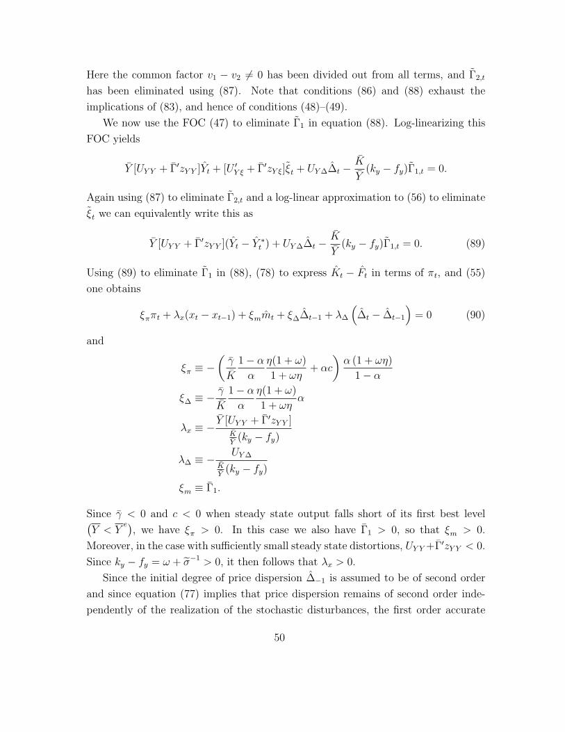
Here the common factor v1 − v2 = 0 has been divided out from all terms, and Γ2,t

has been eliminated using (87). Note that conditions (86) and (88) exhaust the

implications of (83), and hence of conditions (48)–(49).

We now use the FOC (47) to eliminate Γ1 in equation (88). Log-linearizing this

FOC yields

Y [UY Y + Γ′zY Y ]Yt + [U ′Y ξ + Γ′zY ξ]ξt + UY∆∆t −

K

Y(ky − fy)Γ1,t = 0.

Again using (87) to eliminate Γ2,t and a log-linear approximation to (56) to eliminate

ξt we can equivalently write this as

Y [UY Y + Γ′zY Y ](Yt − Y ∗t ) + UY∆∆t −

K

Y(ky − fy)Γ1,t = 0. (89)

Using (89) to eliminate Γ1 in (88), (78) to express Kt − Ft in terms of πt, and (55)

one obtains

ξππt + λx(xt − xt−1) + ξmmt + ξ∆∆t−1 + λ∆

(∆t − ∆t−1

)= 0 (90)

and

ξπ ≡ −(γ

K

1− α

α

η(1 + ω)

1 + ωη+ αc

)α (1 + ωη)

1− α

ξ∆ ≡ − γ

K

1− α

α

η(1 + ω)

1 + ωηα

λx ≡ − Y [UY Y + Γ′zY Y ]KY(ky − fy)

λ∆ ≡ − UY∆

KY(ky − fy)

ξm ≡ Γ1.

Since γ < 0 and c < 0 when steady state output falls short of its first best level(Y < Y

e), we have ξπ > 0. In this case we also have Γ1 > 0, so that ξm > 0.

Moreover, in the case with sufficiently small steady state distortions, UY Y +Γ′zY Y < 0.

Since ky − fy = ω + σ−1 > 0, it then follows that λx > 0.

Since the initial degree of price dispersion ∆−1 is assumed to be of second order

and since equation (77) implies that price dispersion remains of second order inde-

pendently of the realization of the stochastic disturbances, the first order accurate

50

optimal relationship (90) simplifies to

ξππt + λx(xt − xt−1) + ξmmt = 0. (91)

For the sake of brevity, we skip the log-linearization of the FOC (50), which only

serves to determine the value of the Lagrange multiplier γt.

Finally, it remains to log-linearize the FOC (51)

αΦ(Z)′Γt−1 + KαΓ′D(1)Zt + θmt + ψt−1 = 0.

Applying the expectations operator Et−1 to the previous equation, subtracting the

result from it, and using αΓ′D(1) = Γ′ and Γ1 = Γ2 yields

mt =KΓ1

θ

((Kt − Ft

)− Et−1[Kt − Ft]

).

Using once more (78) gives

mt = λm (πt − Et−1[πt]) , (92)

with

λm =KΓ1

θ

α (1 + ωη)

1− α.

Again in with Y < Yeit follows from Γ1 > 0 that λm > 0. Equations (91), (92), and

(82) are those stated in the proposition.

Proof of Proposition 3. We prove that the saddle point properties (7a) and

(7b) hold at the steady state. Continuity then insures that the same applies in a

small enough neighborhood around the steady state.

Since mt = 1 in steady state, inequality in (7a) follows from results derived in

Benigno and Woodford (2005) who show that the Lagrangian (45) is locally concave

(on the set of paths consistent with the model structural relations) near the optimal

steady state if the difference between steady state output and the efficient output

level is sufficiently small.

Since the Lagrangian (45) is locally convex in mt+1 (it contains only terms linear

in mt+1 and the convex term mt+1 logmt+1) the first order conditions for the optimal

choice (92) indeed determine a minimum for the Lagrangian, so that inequality (7b)

also holds.

51

A.3 Proofs for Section 6

To prove proposition 4, we use two auxiliary results, that we prove below:

Lemma 1 Let c be a policy commitment that satisfies Assumptions 1 and 2. Then

under this policy commitment, the equilibrium dynamics of Yt, Πt, Ft, Kt, ∆t are

unaffected to first order by the belief distortions. Moreover, to second order, the

equilibrium dynamics depend at most linearly on the belief distortions mt, but areotherwise independent of them.

Lemma 2 Let c be a policy commitment that satisfies Assumptions 1 and 2. Then

there exists a neighborhood of 1 such that the function Λ(m, c) is a strictly convex

function of m on the domain M, defined as the set of all belief distortions such that

mt+1 remains forever within that neighborhood.

Given these results, we are able to prove the proposition.

Proof of Proposition 4:. For some neighborhood of 1, let M be the set of

belief distortions such that mt+1 remains in this neighborhood at all times; and for

some neighborhood N of the steady-state values of the endogenous variables, let X be

the set of all paths x for the endogenous variables along which the period-t variables

remain within N at all times. Then our local characterization of the upper-bound

solution implies that there exist neighborhoods for which the upper-bound dynamics

x∗ and the associated worst-case belief distortions m∗ solve the problem

minm∈M

maxx∈X

[W (x) + θV (m)] s.t. F (x,m) = 0. (93)

Here x∗ and m∗ refer to the exact solutions to the nonlinear FOCs characterizing the

upper-bound dynamics (rather than to the log-linear approximation to these dynamics

that we have computed); our local analysis above implies that such solutions exist, at

least in the case of a tight enough bound ||ξ|| on the exogenous disturbances, though it

cannot tell us whether these dynamics would also represent a global minmax solution

if we were to relax the bounds on M and X .

Our goal is to show that for an appropriate choice of the bounds that define the

class of policy commitments C, and any outcome function with the property assumed

52

in the proposition,

maxc∈C

minm∈M

[W (O(m, c)) + θV (m)] = minm∈M

maxx∈X

[W (x) + θV (m)] s.t. F (x,m) = 0.

(94)

so that the commitment c∗ that solves this local version of the robustly optimal policy

problem (the problem on the left-hand side of (94)) implements the upper-bound

dynamics. We have already established in section 2.2 the upper bounds

maxc∈C

minm∈M

Λ(m, c) ≤ minm∈M

maxc∈C

Λ(m, c) (95)

≤ minm∈M

maxx∈X

[W (x) + θV (m)] s.t. F (x,m) = 0, (96)

where Λ(m, c) is again shorthand for the objective function in the robustly optimal

policy problem. It therefore suffices for this step of the proof that we establish that

both inequalities hold with equality, under the conditions assumed in the proposition.

This will establish the existence of a c∗ that attains the upper bound; the construction

used to show it will also imply that c coincides with c∗ to a log-linear approximation.

The proof proceeds in stages.

(1) We first establish that (96) holds with equality. We begin by noting that (93)

implies that for suitable bounds M and X , it must be the case that for any m ∈ M,

there exists an allocation xm ∈ X such that F (xm,m) = 0, and

W (xm) + θV (m) ≥ W (x∗) + θV (m∗). (97)

Moreover, there must exist a commitment cm ∈ C that implements the outcome xm

in the case of belief distortions m. Fixing m, for each possible date and state of the

world, let ct ≡ ct(xm), where ct(·) is the function that specifies commitment c at that

date and in that state of the world. Then we can define a policy commitment cm by

a sequence of functions cmt(·), where cmt(x) ≡ ct(x) − ct for each date and each

possible state of the world. The policy commitment cm is, by construction, consistent

with the DEE outcome xm in the case of belief distortions m. We wish to show that

policy cm is also consistent with the existence of a nearby DEE outcome in the case

of any belief distortions that are close enough to m, so that cm is an element of the

class C.Consider the set of (exact, nonlinear) structural equations that define a DEE, in

the case of arbitrary belief distortions m and an arbitrary policy commitment of the

form

ct(x) = ct, (98)

53

for some process ct (not necessarily the one that defines the commitment cm).

When there are no belief distortions and ct = 0 at all times, this system of equations

has a locally unique solution, by condition 2 of Assumption 2, which is equal to the

steady-state values of the endogenous variables if the exogenous disturbances take

their steady-state values. Hence log-linearization of the system around the steady

state (and this policy commitment) must yield a log-linear system with a unique

bounded solution for the endogenous variables in the case of any bounded distur-

bance processes, under the assumption of rational expectations. It follows (since the

conditions for a unique bounded solution are exactly the same when additional ad-

ditive disturbance terms are added to the structural equations) that the log-linear

system also has a unique bounded solution for the endogenous variables in the case of

any bounded processes ξt, mt, ct. This then implies that the original (exact, nonlin-

ear) structural equations have a locally unique solution for the endogenous variables

in the case of any small enough perturbations of the exogenous disturbance process,

the belief distortions, or the process ct that defines the policy commitment.

It is therefore possible to choose the bounds ||ξ||,N ,M tight enough so that (i)

condition (93) holds, and (ii) for any disturbance process satisfying the bound and

any m ∈ M, there is a unique DEE consistent with the policy commitment cm in

which the endogenous variables remain forever within the neighborhood N , and the

allocation associated with this DEE is xm. It follows that for any m ∈ M, the policy

commitment cm defined above belongs to the class C. Moreover, for any outcome

function O(m, c) with the property assumed in the proposition, we must have

O(m, cm) = xm

for any m ∈ M.

It then follows from (97) that

maxc∈C

Λ(m, c) ≥ Λ(m, cm) = W (O(m, cm)) + θV (m) ≥ W (x∗) + θV (m∗)

for any m ∈ M. Hence the minimum value of the left-hand expression (minimizing

over m ∈ M) must also be at least as large as the right-hand expression. Since (96)

asserts that it is also no greater, the two expressions must be equal. This establishes

that (96) holds as an equality.

(2) Before completing the demonstration of (94), we define a policy commitment

c∗ that can be shown to solve the problem on the left-hand side of (94). Let c∗ be

54

the commitment cm (defined above) in the case that m = m∗. It follows from the

discussion above that O(m∗, c∗) = x∗, so that Λ(m∗, c∗) = W (x∗) + θV (m∗). the

minmax value of the problem on right-hand side of (96).

By the definition of the upper-bound solution, x∗ is (at least locally) the best

DEE consistent with belief distortions m∗; then since c∗ achieves this level of the

policymaker’s objective, c∗ must also be a best-response policy commitment within

the class of policies C, so that

maxc∈C

Λ(m∗, c) = Λ(m∗, c∗). (99)

And it is similarly evident that m∗ must be a solution to the outer problem on the

right-hand side of (95).

We further note that, to a log-linear approximation, c∗ is identical to c. Each is a

commitment of the form (98); they differ only to the extent that the process ct is

different in the two cases. In the case of policy c∗, the process ct is obtained as

ct = ct(x∗).

But, by condition 1 of Assumption 2, the functions ct(·) are all consistent with the

upper-bound solution, at least to a log-linear approximation. This implies that in that

log-linear approximation, ct = 0 at all times. Hence in the log-linear approximation,

c and c∗ are identical policies.

(3) Finally, we establish that (95) holds with equality as well, and that c∗ is a

policy commitment that achieves the upper bound. Given the results of step (2) of

the proof, we can alternatively write the proposition that we wish to establish as

maxc∈C

minm∈M

Λ(m, c) = Λ(m∗, c∗). (100)

Moreover, it will suffice to prove that

minm∈M

Λ(m, c∗) = Λ(m∗, c∗). (101)

For we already know from (95) that there exists no commitment c for which minm Λ(m, c)

is larger than Λ(m∗, c∗); since (101) suffices to ensure that the bound can be obtained,

it will imply (100). Furthermore, it implies that c∗ is a policy commitment that

achieves the bound.

55

Let us define the function

Ω(m) ≡ maxc∈C

Λ(m, c)

for arbitrary m ∈ M. It follows from the discussion in step (2) that

minm∈M

Ω(m) = Ω(m∗) = Λ(m∗, c∗),

and hence that

Ωm(m∗) = 0.

But by the envelope theorem, Ωm(m∗) = Λm(m

∗, c∗), so that we must have

Λm(m∗, c∗) = 0. (102)

Finally, let us consider the function Λ∗(m) ≡ Λ(m, c∗), also defined for arbitrary

m ∈ M. We wish to show that m∗ minimizes this function (at least locally). By

(102), m∗ is a critical point of the function, so it suffices to show that Λ∗(m) is a

strictly convex function of m, at least for m in a neighborhood of m∗. By Lemma 2,

Λ(m, c) is (at least locally) a strictly convex function, for any commitment c satisfy-

ing Assumptions 1 and 2. But we have shown that c∗ is an example of a commitment

satisfying Assumptions 1 and 2, and so the lemma can be applied. It follows that

Λ∗(m) is a strictly convex function of m, for m in some neighborhood of the undis-

torted beliefs. By choosing tight enough bounds ||ξ||, we can ensure that m∗ is in the

neighborhood on which the function is strictly convex, and hence it is strictly convex

in a neighborhood of m∗.

This establishes that we can define the bounds so that (101) holds, from which

(100) follows. It then follows directly that (95) holds with equality, and that the

commitment c∗ defined in step (2) is an example of a policy that solves the local

robust policy problem. Hence c is equivalent, to a log-linear approximation, to the

solution to the local robust policy problem, and the value of the objective achieved by

the locally robustly optimal policy is the one achieved by the upper-bound solution.

We now prove Lemmas 1 and 2, required for the above proof. (The proof of

Proposition 4 relies upon Lemma 2, which in turn relies upon Lemma 1.) We first

note that a DEE consistent with a policy commitment c of the kind assumed in

56

the lemmas, and with given belief distortions m, corresponds to a set of processes

Yt, Ft, Kt, it,∆t∞t=0 satisfying the conditions

uY (Yt; ξt) = βEt

[mt+1uY (Yt+1; ξt+1)

1 + itΠt+1

1− gt1− gt+1

](103)

Ft = f(Yt; ξt) + αβEt

[mt+1Π

η−1t+1Ft+1

](104)

Kt = k(Yt; ξt) + αβEt

[mt+1Π

η(1+ω)t+1 Kt+1

](105)

∆t = h(∆t−1, Kt/Ft) (106)

Etmt+1 = 1

ct(·) = 0 (107)

for all t.

The problem defining worst-case belief distortions in the case of the policy c is

then

minmt+1,Yt,Ft,Kt,it,∆t∞t=0

E0

∞∑t=0

βt [U(Yt,∆t; ξt) + θβmt+1 logmt+1] (108)

+ αΓ′−1Φ(Z0) (109)

subject to constraints (103)–(107), where αΓ′−1Φ(Z0) captures an initial precommit-

ment to achieve a time-invariant solution, as in problem (45). In the case of a policy

commitment c satisfying Assumptions 1 and 2, there will be a locally unique DEE

(solution to equations (103)–(106) and (107)) in the case of any given small enough

belief distortions m, and this will have to be the allocation given by the outcome

function. The value of the objective function in (109) for those belief distortions will

then define the objective Λ(m, c) in our reduced-form statement of the robustly opti-

mal policy problem. Lemmas 1 and 2 state some properties of local approximations

to the solutions to these equations.

Proof of Lemma 1:. We first prove that the solution for the endogenous

variables Yt, Πt, Ft, Kt, ∆t, in the case of arbitrary (small) belief distortions, is

unaffected by the belief distortions up to first order. To do so, we linearize the

system of nonlinear equations listed above.

57

Defining the exogenous process Yt =Ct

1−gtand noting that uY (Yt; ξt) = (Yt/Yt)

−1/σ (1− gt),

we can rewrite equation (103) as(Yt

Y t

)−1/σ

= βEt

[mt+1

(Yt+1

Y t+1

)−1/σ1 + itΠt+1

].

Denoting exogenous terms by e.t., using Etmt+1 = 0 and (1 + ı)β = 1, a linear

approximation to this equation is given by

− σ−1

YYt = Et[−

σ−1

YYt+1 + βıt − Πt+1] + e.t.+O(∥ξ∥2). (110)

Next, we linearize (104) and (105):

Ft = fY Yt + αβEt

[(η − 1)F Πt+1 + Ft+1

]+ e.t+O(∥ξ∥2) (111)

Kt = kY Yt + αβEt

[(η(1 + ω))KΠt+1 + Kt+1

]+ e.t.+O(∥ξ∥2). (112)

Subtracting the first from the second equation and using K = F

Kt − Ft = (kY − fY ) Yt + αβEt

[(1 + ηω)KΠt+1 +

(Kt+1 − Ft+1

)]+ e.t+O(∥ξ∥2).

A linear approximation to (106) delivers

Πt =(1− α)

α

1

1 + ωη

1

K

(Kt − Ft

)+O(∥ξ∥2),

so that

Πt = (kY − fY )1− α

K (1 + ωη)αYt + βEt

[Πt+1

]+ e.t+O(∥ξ∥2). (113)

Note that equations (110)-(113) are independent of the belief distortions up to first

order, and thus identical as in the case with rational private sector expectations.

Since the policy commitment c is also assumed independent of the belief distortions

and because c insures a locally determinate outcome under rational expectations,

equations (110)-(113) have a locally unique solution that — to first-order accuracy

— is independent of the belief distortions.

We now show that to second order, the solution forYt, Πt, Ft, Kt, ∆t

depends

only linearly on mt. Since up to first order the solutionYt, Πt, Ft, Kt, ∆t

evolves

58

independently of the belief distortions, a quadratic approximation to equation (103)

is given by

− σ−1

YYt = Et[−

σ−1

YYt+1 + βıt − Πt+1 −

σ−1

YYt+1mt+1 − Πt+1mt+1 +

σ−1

YY t+1mt+1]

+ t.i.m+ e.t.+O(∥ξ∥3).

The only new terms appearing in a quadratic approximation are thus either indepen-

dent of the belief distortions (as they involve squares of the variables Yt, Πt, Ft, Kt, ∆t

and exogenous terms) or of the form EtXt+1mt+1, where Xt+1 is a variable indepen-

dent of the belief distortions. The same can be noted when quadratically approxi-

mating (104), (105) and (106). Moreover, a quadratic approximation to the policy

commitment involves no terms in m. We can thus perform the same steps as in the lin-

earization above and solve for a unique non-explosive solution forYt, Πt, Ft, Kt,∆t

,

which is accurate to second order. The only newly appearing terms will be t.i.m and

terms linear in m, which completes the proof.

Proof of Lemma 2:. Let c be a policy commitment satisfying Assumptions

1 and 2. The problem defining worst-case belief distortions is then given by (109).

When the exogenous disturbances take their steady-state values at all times, the

locally unique DEE consistent with zero belief distortions is given by the steady

state. We wish to consider the value Λ(m, c) of the objective in (109) in the case

that both belief distortions and the exogenous disturbances are small; in such a case,

the DEE allocation will be correspondingly close to the steady state. We locally

approximate Λ(m, c) through Taylor series expansions around the steady-state values

of all variables.

From Lemma 1 we know that the variables (Yt, Πt, Ft, Kt, ∆t) are to first order

independent of the belief distortions. A second-order accurate approximation of the

objective function in problem (109) is thus given by

E0

∞∑t=0

βt[U(Yt,∆t; ξt) + θβmt+1 logmt+1 + αΓ′

−1Φ(Z0)]

= E0

∞∑t=0

βt

[UY Yt + U∆∆t +

1

2θβ (mt+1)

2 + αΓ′−1D(1)

(F0

K0

)]+ t.i.m+O(∥ξ∥3), (114)

59

where t.i.m refers to (first- and higher-order) terms that are independent of the

belief distortion process m. Lemma 1 also implies that the endogenous variablesYt, ∆t, F0, K0

showing up in (114) depend up to second-order accuracy only linearly

on the chosen process for the belief distortions mt+1, but are otherwise independentof the choices of the belief distortions (to second-order accuracy). Strict convexity

of (114) is thus implied by the quadratic term in m, so that second-order conditions

for the worst-case belief distortions problem necessarily hold at the solution to the

first-order conditions.

Proof of corollary 3:. Suppose policy commits to the targeting rule (71) from

date t onwards. To establish determinacy of the solution under rational expectations

with such a commitment, we have to analyze the system of equations

ξππt+j + λx(xt+j − xt+j−1) + ξmλm (πt+j − Et+j−1[πt+j]) = 0 (115)

πt+j − κxt+j − βEt+jπt+j+1 − ut+j = 0, (116)

which holds for all j ≥ 0. Taking the expectation Et−1[·] and rearranging terms

delivers a system describing the dynamics of the t − 1 dated expectations of the

endogenous variables(Et−1πt+j

Et−1xt+j

)=

(β−1

(1 + κ ξπ

λx

)−κ

β

− ξπλx

1

)(Et−1πt+j

Et−1xt+j−1

)+

(−β−1

0

)Et−1ut+j.

Under the additional assumptions stated in the corollary, we have λx > 0, λπ > 0,

and κ > 0, so that the characteristic polynomial of the autoregressive matrix in the

preceding equation implies that both roots are positive with one root being explosive

and one being stable. Since Et−1xt−1 is predetermined at date t, the previous equation

system has a unique non-explosive solution for the dynamics of Et−1Πt+j and Et−1xt+j

for all j ≥ 0, given any bounded path for Et−1ut+j for all j ≥ 0. Repeating this

procedure for any date h ≥ t − 1 determines also unique non-explosive values for

EhΠt+j and Ehxt+j for all j > h − t. Taking the expectation Et−1[·] of equations(115) and (116) and subtracting the corresponding results from equations (115) and

(116), respectively, delivers for j = 0

(ξπ + ξmλm) (πt − Et−1[πt]) + λx(xt − Et−1xt) = 0

πt − Et−1[πt]− κ(xt − Et−1xt)− β (Etπt+1 − Et−1πt+1)− (ut − Et−1ut) = 0,

60

which uniquely determines πt and xt as a linear function of the already determined ex-

pectations (Et−1πt, Et−1πt+1, Etπt+1, Et−1xt) and the exogenous terms (ut+j−Et−1ut+j).

Repeating this last step for each j > 0 determines the locally unique state contingent

path for πt+j, xt+j and completes the proof of local determinacy of the outcome

under rational expectations.

A.4 Proofs for Section 7.1

Derivation of the best response dynamics (74). Equation (73) implies

ξππt = −λx(xt − xt−1)− ξmmt (117)

and substituting into (72)delivers

Et

(βxt+1 − (1 + β +

ξπκ

λx)xt + xt−1

)=ξπλxut +

ξmλxmt. (118)

The lag polynomial on the l.h.s. can be expressed as

L

(βL−2 − (1 + β +

ξπκ

λx)L−1 + 1

)= −βe1(1− (e1L)

−1)(1− e2L),

where e1 and e2 solve βe2 − (1 + β + ξπκλx

)e + 1 and satisfy e1 > β−1 and e2 ∈ (0, 1).

Using the lag polynomial, we can write (118) as

−βe1Et

[(1− (e1L)

−1)(1− e2L)xt]=ξπλxut +

ξmλxmt

−βe1(1− e2L)xt =ξπλxEt

[(1− (e1L)

−1)−1ut]+ξmλxEt

[(1− (e1L)

−1)−1mt

].

Assuming that ut evolves according to (61) and using Et[mt+j] = 0 for all j ≥ 1 we

have

−βe1(1− e2L)xt =ξπλx

1

1− ρ/e1ut +

ξmλxmt.

Solving for x1 gives

xt = e2xt−1 −ξπβλx

1

e1 − ρut −

1

e1

ξmβλx

mt,

which is the upper row in (74). Substituting this into (117) delivers the lower row in

(74).

61

Proof of Proposition 6. Let m denote a state contingent belief distortion and

π a state contingent inflation commitment. Similarly, let (m∗, π∗) the corresponding

contingent sequences of the the upper bound solution. Letting BR denote the best

response function for inflation, we have that π∗ = BR(m∗). Furthermore, letting

O(π,m) denote the objective function of the policymaker, we know from corollary 1

that

O(π∗,m∗) < O(π∗,m),

for all m = m∗. Since

O(π∗,m) ≤ maxπ

O(π,m) = O(BR(m),m),

this implies that

O(π∗,m∗) < O(BR(m),m)

for all m = m∗. This shows that the worst-case belief distortions are given by m∗

whenever the policymaker has committed to the best-response function BR(·).

A.5 Proofs for Section 7.2

Proof of Proposition 7. Consider problem (75). The first-order condition for it−1

is given by

Et−1[Ωtmt+1uY (Yt+1; ξt+1)1

Πt+1

1 + gt1 + gt+1

] = 0

and linearizing this around the optimal steady state where Ω = 0 delivers

Et−1

[Ωt

]= 0. (119)

The first order condition for mt is given by

θ(1 + logmt) + αΓ′t−1Φ(Zt) + ψt−1 + Ωt−1uY (Yt; ξt)

1 + it−2

Πt

1 + gt−1

1 + gt= 0

and its linearization by

θmt + αKΓ′D(1)Zt + αΦ(Z)′Γt−1 + ψt−1 + β−1Ωt−1 = 0.

Applying the operator Et−1 [·] to this equation, subtracting the result from it and

using (119) gives

θmt + αKΓ′D(1)

(Zt − Et−1Zt

)= 0.

Using a log-linearization of (37) then delivers (59).

62