Robust Two-Stage Least Squares: some Monte Carlo experiments · estimators. Unlike the Three-Stage...
24
Munich Personal RePEc Archive Robust Two-Stage Least Squares: some Monte Carlo experiments Mishra, SK North-Eastern Hill University, Shillong (India) 26 July 2008 Online at https://mpra.ub.uni-muenchen.de/9737/ MPRA Paper No. 9737, posted 29 Jul 2008 07:23 UTC
Transcript of Robust Two-Stage Least Squares: some Monte Carlo experiments · estimators. Unlike the Three-Stage...

Munich Personal RePEc Archive
Robust Two-Stage Least Squares: some
Monte Carlo experiments
Mishra, SK
North-Eastern Hill University, Shillong (India)
26 July 2008
Online at https://mpra.ub.uni-muenchen.de/9737/
MPRA Paper No. 9737, posted 29 Jul 2008 07:23 UTC

Robust Two-Stage Least Squares: Some Monte Carlo Experiments
SK Mishra
Department of Economics
North-Eastern Hill University
Shillong (India)
1. Introduction: The Two-Stage Least Squares (2-SLS) is a well known econometric technique
used to estimate the parameters of a multi-equation (or simultaneous equations) econometric
model when errors across the equations are not correlated and the equation(s) concerned is
(are) over-identified or exactly identified. It is one of the members of the family of k-class
estimators. Unlike the Three-Stage Least Squares, it does not estimate the parameters of all the
equations of the model in one go. The 2-SLS estimates the parameters of an econometric model
equation by equation, that is, one equation at a time.
Let a multi-equation econometric model be described by the system of its structural equations
0,YA XB U+ + = where Y is an n m× data matrix of m endogenous variables in n observations,
X is an n k× data matrix of k exogenous or pre-determined variables in n observations, A is
an m m× full rank matrix of unknown parameters or coefficients associated with ,Y B is a k m×
matrix of unknown parameters or coefficients associated with X and U is an n m× matrix of
(unobserved) errors. The elements of A and B are called the structural parameters. Since U is
often correlated with Y which is itself stochastic, the parameters in the columns of A and B
cannot be estimated by means of the Ordinary Least Squares (OLS) in view of the violation of the
Gauss-Markov assumptions for the applicability of the OLS. Instead of using the OLS directly, the
system of equations 0YA XB U+ + = is first transformed into the reduced form equations. The
reduced form equations describe Y in terms of X only. Indeed if we post-multiply the system
of equations 0YA XB U+ + = by 1,A− we have 1 1 1 0YAA XBA UA− − −+ + = or ,Y XP E= + where
1P BA
−= − and 1.E UA−= − Now since X is fixed (non-stochastic) and it cannot be correlated
with ,E the system of reduced form equations Y XP E= + is amenable to estimation by the OLS.
Therefore, P (which is the matrix of the reduced form coefficients) is estimated by the OLS as 1ˆ [ ]P X X X Y
−′ ′= and used to obtain ˆ ˆ.Y XP= Then in each equation where any endogenous
variable jY Y⊂ appears as an explanatory variable, jY is replaced by ˆjY . Due to this
replacement, the explanatory variables are no longer stochastic or correlated with the error
term in the equation concerned, and so the equation is amenable to estimation by the OLS.
Application of the OLS (once again) on this transformed equation readily gives the estimates of
the parameters in that equation.
2. Implications of the Presence of Outliers in the Data Matrices: Now suppose there are some
outliers in ,X Y or both the data matrices. This would affect 1ˆ [ ]P X X X Y−′ ′= and consequently
ˆ ˆ.Y XP= At the second stage since ˆ ˆjY Y⊂ appear as explanatory variables, all the estimated
parameters would be affected. As a matter of fact, the effects of outliers will pervade through
all the equations and the estimated structural parameters in them. These effects are so
intricately pervasive that it is very difficult to assess the influence of outliers on the estimated
structural parameters.

2
A number of methods have been proposed to obtain robust estimators of regression parameters
but most of them are limited to single equation models. Their adaptation to estimation of the
structural parameters of multi-equation models is not only operationally inconvenient, it is also
theoretically unconvincing. Moreover, generalization of those methods to multi-equation cases
has scarcely been either successful or popular.
3. The Objectives of the Present Study: In this study a method has been proposed to
conveniently generalize the 2-SLS to the weighted 2-SLS (W2-SLS) so that 1ˆ [( ) ( )] ( ) ( ),P wX wX wX wY
−′ ′= where w is the weight matrix applied to Y and .X Accordingly, we
have ˆ ˆ.Y XP= At the 2nd
stage, for the thi equation we have 1[( ) ( )] ( ) ( ),i i i i i i i i ig Z Z Z yω ω ω ω−′ ′=
where ˆ ˆ ˆ ˆˆ[ | ] ; [ | ]; ; ; ;i i i i i i i i i ig a b Z Y X y Y Y Y y Y′= = ⊂ ⊂ ∉ iX X⊂ ; iy is the observed endogenous
variable appearing in the thi structural equation as the dependent variable, ˆiY is the set of
estimated endogenous variables appearing in the thi equation as the explanatory variables and
iX is the set of exogenous (or predetermined) variables appearing in the thi equation as the
explanatory variables. It may be noted that at the second stage of the proposed W2-SLS we use
different weights ( )ω for different equations. These weights ( w and iω ) are obtained in a
particular manner as described latter in this paper. We also conduct some Monte Carlo
experiments to demonstrate that our proposed method performs very well in estimating the
structural parameters of multi-equation econometric models while the data matrices are
containing numerous large outliers.
4. Determination of Weights in the Weighted Two-Stage Least Squares: Using the Mahalanobis
distance as a measure of deviation from center, Campbell (1980) obtained a robust covariance
matrix that is almost free from the influence of outliers. Campbell’s method is an iterative
method. Given an observed data matrix, Ζ , in n observations (rows) and v variables (columns)
it obtains a v -elements vector of weighted (arithmetic) mean, ,z and weighted variance-
covariance matrix, ( , ),S v v in the following manner. Initially, all weights, ; 1, nϖ =
�� are
considered to be equal, ,/1 n and the sum of weights, 1
1.n
ϖ=
=� �� Further, we define
0 1 1 2/ 2; 2, 1.25.d v β β β= + = =
Then we obtain
1 1/
n nz zϖ ϖ
= ==� �� � �� �
2 2
1 1( ) ( ) / 1
n nS z z z zϖ ϖ
= =� �′= − − −� �� �� � � �� �
{ }
1/ 21( ) ( ) ; 1,d z z S z z n− ′= − − =
� � ��
( ) / ; 1, :d d nϖ ϖ= =� � �
�2 2
0 0 0 2( ) ( ) exp[ 0.5( ) / ].d d if d d else d d d dϖ ϖ β= ≤ = − −� � � � �
If 0d ≅�
then 1.ϖ =�
We will call it the original Campbell procedure to obtain a robust
covariance matrix. However, our experience with this procedure to obtain a robust covariance
matrix is not very encouraging in this study as well as elsewhere (Mishra, 2008). We will use the
acronym OCP for this original Campbell procedure.
Hampel et al. (1986) defined the median of absolute deviations (from median) as a measure of
scale, ( ) | ( ) |H a a as z median z median z= −� �
� �
which is a very robust measure of deviation. Using

3
this measure of deviation also, we may assign weights to different data points. If we choose to
heuristically assign the weight 1ϖ =� for ( ) ( ),
H Hd s d d d s d− ≤ < +� � �
2(1/ 2)ϖ =
� for
2 ( ) ( )H H
d s d d d s d− ≤ < −� � �
as well as 2 ( ) ( )H H
d s d d d s d+ ≥ > +� � �
and so on, and use
Campbell’s iterative method incorporating these weights, we may obtain a robust covariance
matrix and weights. Our experience with this procedure has been highly rewarding in this study
as well as elsewhere (Mishra, 2008). We will call it the Modified Campbell Procedure (MCP) to
obtain a robust covariance matrix and weights to different data points.
The weights ( )ϖ obtained through the MCP (or OCP, as the case may be) are used as w in
1ˆ [( ) ( )] ( ) ( )P wX wX wX wY−′ ′=
at the first stage of the W2-SLS to obtain the robust estimates of
the matrix of reduced form coefficients. In this procedure of obtaining ˆ,P X contains the
unitary vector to take care of the intercept term, although weights ( )w ϖ= are obtained with *Z
that contains Y and all the variables in ,X sans the unitary vector relating to the intercept term.
Similarly, at the second stage, the MCP/OCP weights ( )i iω ϖ= are obtained from
* *ˆ[ | | ],i i iZ y Y X= where *iX contains all exogenous (predetermined) variables appearing in the
thi structural equations, sans the unitary vector related to the intercept term. However, in
obtaining [ | ]i i ig a b ′= , the matrix ˆ[ | ]i i iZ Y X= is used wherein iX contains all exogenous
(predetermined) variables, including the one related to the intercept term in the thi equation.
5. Some Monte Caro Experiments: In order to assess the performance of our proposed method
and compare it with the 2-SLS when data matrices (Y and X ) contain outliers, we have
conducted some Monte Carlo experiments. Using the random number generator seed=1111, we
have generated X containing five exogenous variables in 100 observations and appended to it
the 6th
column of unitary vector to take care of the intercept term. Thus, in all, we have X in
100 rows and 6 columns. All values of X lie between 0 and 20 such that 0 20.ijx< < Then the
data matrix for endogenous variables, ,Y has been generated with the parameter matrices, A
and B and adding a very small normally distributed random error, (0,0.001)U N� directly,
without going into the subtleties of obtaining .U EA= − The magnitude of error has been kept at
a very low level since our objective is not to mingle the effects of errors with those of outliers
on the estimated parameters. If the magnitude of errors is large, it would affect the estimated
values of parameters and it would be difficult to disentangle the effects of outliers from those of
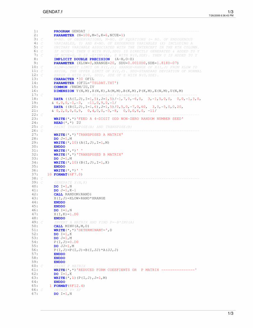
the errors. The computer program GENDAT (in FORTRAN 77) to generate data is appended. As
already mentioned, the program was run with the random number generator seed = 1111. The
following are the matrices of structural parameters used in our experiments.
-1 7 0 -6 0 0 5 0 -7 0 60
3 -1 5 0 0
0 0 -1 3 0 ;
6 0 0 -1 -3
-11 0 9 0 -1
A B
� �� �� �� �′ ′= =� �� �� �� �
3 0 -5 0 0 20
0 2 0 0 0 9
0 4 0 0 -3 -8
0 0 0 6 0 -11
� �� �� �� �� �� �� �� �
The data (Y and X ) thus generated are used as the base data to which different number and
different sizes of perturbation quantities are added in different experiments. For every
experiment we have limited the number of replicates (NR) to 100, although this number could

4
have been larger or smaller. For each experiment the mean, standard deviation and RMS (Root-
Mean-Square) of expected parameters ( A and B ) have been computed over the 100 replicates.
The following formulas are used for computing these statistics.
1 1
ˆ ˆˆ ˆ( ) (1/ ) ; , 1, ; ( ) (1/ ) ; 1, ; 1,NR NR
ij ij ij ijMean a NR a i j m Mean b NR b i k j m= =
= = = = =� �� �� �
0.5 0.52 2 2 2
1 1
1 1ˆ ˆ ˆˆ ˆ ˆ( ) ( ) ( ) ; , 1, ; ( ) ( ) ( ) ; 1, ; 1,NR NR
ij ij ij ij ij ijSD a a Mean a i j m SD b b Mean b i k j mNR NR= =
� � � �= − = = − = =� � � �� � � �� �� �� �
0.5 0.52 2
1 1
1 1ˆ ˆˆ ˆ( ) ( ) ; , 1, ; ( ) ( ) ; 1, ; 1,NR NR
ij ij ij ij ij ijRMS a a a i j m RMS b b b i k j mNR NR= =
� � � �= − = = − = =� � � �� � � �� �� �� �
A distance between RMS and SD entails bias of the estimation formula and a larger SD entails
inefficiency of the estimation formula. Reduction in SD as a response to increase in the number
of replicates entails consistency of the estimator formula. In the present exercise we have not
looked into the consistency aspect by fixing the number of replicates (NR) to 100, although it
could have been done without much effort by increasing NR from (say) 20 to 200 (or more) by
an increment of 20 or so.
Experiment-1: In this experiment we have set the number of perturbations at 10 (i.e. NOUT=10)
and the size of perturbation (OL) in the range of 10 25± or between -15 to 35. In this range the
size of perturbation quantities is randomly chosen and those quantities are added to the data at
equiprobable random locations. Accordingly, in the program ROB2SLS the parameters are set at
OMIN=10, OMAX=50 such that OL=OMIN+(OMAX-OMIN)*(RAND-0.5). The random number
RAND lays between zero and unity (exclusive of limits). To generate the random numbers seed =
2211 has been used (in this as well as subsequent experiments). With this design, we have
estimated the structural parameters by 2-SLS, OCP and MCP. The results are presented in tables
1.1 through 3.3.
Table-1.1. Mean of Estimates of Structural Parameters: Method –2-SLS
Variables/
Equations
Mean of Estimated A Matrix Mean of Estimated B Matrix
1y 2y 3y 4y 5y 1x 2x 3x 4x 5x 6x
Eq-1 ��� ������� � ����� � � ����� � ����� � � ��������
Eq-2 ������ ��� ������ � � ����� � � ����� �� � � ����� ��
Eq-3 � � ��� ������ � � ������ � � � ����� �
Eq-4 ����� � � ��� ����� � ���� � � � ��� �� ��� ���
Eq-5 ������� � ������ � ��� � � � ������� � �������
.
Table-1.2. Standard Deviation of Estimates of Structural Parameters: Method –2-SLS
Variables/
Equations Standard Dev of Estimated A Matrix Standard Dev of Estimated B Matrix
1y 2y 3y 4y 5y 1x 2x 3x 4x 5x 6x
Eq-1 � ������ � ������ � � ������ � ��� ��� � ������
Eq-2 ������ � �� ��� � � ������ � ������ � � ������
Eq-3 � � � ���� � � � ����� � � � �����
Eq-4 ������ � � � ����� � ���� �� � � ������ �����
Eq-5 ����� � ������ � � � � � ��� � � �����
.

5
Table-1.3. Root Mean Square of Estimates of Structural Parameters: Method –2-SLS
Variables/
Equations RMS of Estimated A Matrix RMS of Estimated B Matrix
1y 2y 3y 4y 5y 1x 2x 3x 4x 5x 6x
Eq-1 � ����� � �� � � � ������� � ��� �� � ��� ����
Eq-2 �� �� � �� ��� � � ������ � ����� � � ������
Eq-3 � � � ������ � � ������ � � � �������
Eq-4 ������� � � � ������ � ������� � � ��� �� �����
Eq-5 ���� � ������ � � � � � ����� � � �� �� �
.
Table-2.1. Mean of Estimates of Structural Parameters: Method –W2-SLS (OCP)
Variables/
Equations
Mean of Estimated A Matrix Mean of Estimated B Matrix
1y 2y 3y 4y 5y 1x 2x 3x 4x 5x 6x
Eq-1 ��� ������ � �������� � � �� ���� � ������� � � ������
Eq-2 ������ ��� ������ � � ������� � ���� �� � � ��� ����
Eq-3 � � ��� �� ��� � � �� ��� � � � �����
Eq-4 ����� � � ��� ����� �� � ������� � � �������� ���� � �
Eq-5 ������� � ������� � ��� � � � �� � � ����� �
.
Table-2.2. Standard Deviation of Estimates of Structural Parameters: Method –W2-SLS (OCP)
Variables/
Equations Standard Dev of Estimated A Matrix Standard Dev of Estimated B Matrix
1y 2y 3y 4y 5y 1x 2x 3x 4x 5x 6x
Eq-1 � ���� � � ������ � � ����� � ������� � �������
Eq-2 ������ � ����� � � ����� � ����� � � � ������
Eq-3 � � � ������� � � ��� �� � � � ��� ��
Eq-4 ������ � � � ������� � ���� � � � ���� ��� ���
Eq-5 �������� � ������ � � � � � ���� � � ����� �
.
Table-2.3. Root Mean Square of Estimates of Structural Parameters: Method –W2-SLS (OCP)
Variables/
Equations RMS of Estimated A Matrix RMS of Estimated B Matrix
1y 2y 3y 4y 5y 1x 2x 3x 4x 5x 6x
Eq-1 � ������ � �� � �� � � ���� �� � �� �� � � ��� ����
Eq-2 ������� � ������ � � ������ � �� �� � � �� � ��
Eq-3 � � � ������ � � ����� � � � � ��� ��
Eq-4 �� ��� � � � �� ���� � ����� � � ������ ������
Eq-5 �������� � ������� � � � � � � � �� � �������
.
Table-3.1. Mean of Estimates of Structural Parameters: Method –W2-SLS (MCP)
Variables/
Equations
Mean of Estimated A Matrix Mean of Estimated B Matrix
1y 2y 3y 4y 5y 1x 2x 3x 4x 5x 6x
Eq-1 ��� ����� � � ��� � � ��� �� � ������� � �����
Eq-2 ���� ��� ����� � � ���� � ������ � � ����
Eq-3 � � ��� ������� � � ������� � � � ������
Eq-4 ������� � � ��� ������� � ������� � � ����� � ����� ��
Eq-5 ������ � ���� � ��� � � � ������� � �������
.

6
Table-3.2. Standard Deviation of Estimates of Structural Parameters: Method –W2-SLS (MCP)
Variables/
Equations Standard Dev of Estimated A Matrix Standard Dev of Estimated B Matrix
1y 2y 3y 4y 5y 1x 2x 3x 4x 5x 6x
Eq-1 � � �� � ��� � � ���� � ���� � ����
Eq-2 ��� � ��� � � ��� � ��� � � ����
Eq-3 � � � ��� � � ��� � � � ���
Eq-4 ��� � � � ��� � �� � � � ���� ����
Eq-5 ���� � ��� � � � � � � � � ���
.
Table-3.3. Root Mean Square of Estimates of Structural Parameters: Method –W2-SLS (MCP)
Variables/
Equations RMS of Estimated A Matrix RMS of Estimated B Matrix
1y 2y 3y 4y 5y 1x 2x 3x 4x 5x 6x
Eq-1 � ���� � ���� � � �� �� � ��� � � �����
Eq-2 ��� � ���� � � ��� � ���� � � �� �
Eq-3 � � � ��� � � ��� � � � ���
Eq-4 ���� � � � ���� � ��� � � ���� ����
Eq-5 ���� � ��� � � � � � � � � ����
A perusal of these table immediately reveals that the 2-SLS and the W2-SLS(OCP) perform very
poorly. Of the two, the 2-SLS appears to perform somewhat better. However, the performance
of the W2-SLS(MCP) is excellent.
Experiment-2: In this experiment we have set the number of perturbations at 10 (i.e. NOUT=10)
and the size of perturbation (OL) in the range of 10 50± or between -40 to 60. The parameters in
the program are set at OMIN=10, OMAX=100 and hence OL=OMIN+(OMAX-OMIN)*(RAND-0.5).
The dismal performance of 2-SLS and W2-SLS(OCP) observed in experiment-1 has been further
aggravated and therefore we do not consider it necessary to report the mean, SD and RMS of
estimated structural parameters for those estimators. However, once again the W2-SLS(MCP)
has performed exceedingly well and the results have been presented in Tables 4.1 through 4.3.
Table-4.1. Mean of Estimates of Structural Parameters: Method –W2-SLS (MCP)
Variables/
Equations
Mean of Estimated A Matrix Mean of Estimated B Matrix
1y 2y 3y 4y 5y 1x 2x 3x 4x 5x 6x
Eq-1 ��� ����� � � ����� � � ��� �� � ������� � �����
Eq-2 ���� ��� ����� � � ���� � ������ � � �����
Eq-3 � � ��� ������� � � �� � � � ���� �
Eq-4 ������� � � ��� ������� � ������� � � ����� � ����� ��
Eq-5 ������ � ���� � ��� � � � ������� � �������
.
Table-4.2. Standard Deviation of Estimates of Structural Parameters: Method –W2-SLS (MCP)
Variables/
Equations Standard Dev of Estimated A Matrix Standard Dev of Estimated B Matrix
1y 2y 3y 4y 5y 1x 2x 3x 4x 5x 6x
Eq-1 � � �� � �� � � � ���� � � �� � �����
Eq-2 ��� � ��� � � ��� � ��� � � ���
Eq-3 � � � ��� � � ��� � � � ���
Eq-4 ��� � � � ��� � ���� � � ��� ����
Eq-5 ���� � ��� � � � � � � � � ���
7
.
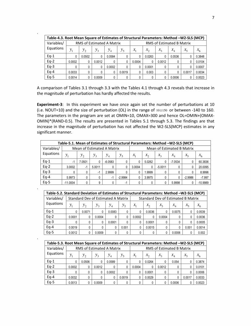
Table-4.3. Root Mean Square of Estimates of Structural Parameters: Method –W2-SLS (MCP)
Variables/
Equations RMS of Estimated A Matrix RMS of Estimated B Matrix
1y 2y 3y 4y 5y 1x 2x 3x 4x 5x 6x
Eq-1 � ���� � ���� � � �� �� � ��� � � ����
Eq-2 ��� � ���� � � ��� � ���� � � ����
Eq-3 � � � ��� � � ��� � � � ���
Eq-4 ���� � � � ���� � ��� � � ���� ����
Eq-5 ���� � ��� � � � � � � � � ����
A comparison of Tables 3.1 through 3.3 with the Tables 4.1 through 4.3 reveals that increase in
the magnitude of perturbation has hardly affected the results.
Experiment-3: In this experiment we have once again set the number of perturbations at 10
(i.e. NOUT=10) and the size of perturbation (OL) in the range of 10 150± or between -140 to 160.
The parameters in the program are set at OMIN=10, OMAX=300 and hence OL=OMIN+(OMAX-
OMIN)*(RAND-0.5). The results are presented in Tables 5.1 through 5.3. The findings are that
increase in the magnitude of perturbation has not affected the W2-SLS(MCP) estimates in any
significant manner.
Table-5.1. Mean of Estimates of Structural Parameters: Method –W2-SLS (MCP)
Variables/
Equations
Mean of Estimated A Matrix Mean of Estimated B Matrix
1y 2y 3y 4y 5y 1x 2x 3x 4x 5x 6x
Eq-1 ��� ����� � � ���� � � ��� �� � ������� � ��� �
Eq-2 ���� ��� ����� � � ���� � ������ � � �����
Eq-3 � � ��� ������� � � ������� � � � ���� �
Eq-4 ������� � � ��� ������� � ������� � � ����� � �������
Eq-5 ������ � �� � ��� � � � ������ � �������
.
Table-5.2. Standard Deviation of Estimates of Structural Parameters: Method –W2-SLS (MCP)
Variables/
Equations Standard Dev of Estimated A Matrix Standard Dev of Estimated B Matrix
1y 2y 3y 4y 5y 1x 2x 3x 4x 5x 6x
Eq-1 � ���� � ��� � � �� � � ���� � �����
Eq-2 ��� � ��� � � ��� � ��� � � �� �
Eq-3 � � � ��� � � ��� � � � ���
Eq-4 ���� � � � ��� � ���� � � ��� ����
Eq-5 ���� � ��� � � � � � � � � ���
.
Table-5.3. Root Mean Square of Estimates of Structural Parameters: Method –W2-SLS (MCP)
Variables/
Equations RMS of Estimated A Matrix RMS of Estimated B Matrix
1y 2y 3y 4y 5y 1x 2x 3x 4x 5x 6x
Eq-1 � �� � � ���� � � �� �� � ���� � �����
Eq-2 ��� � ���� � � ��� � ���� � � ����
Eq-3 � � � ��� � � ��� � � � � �
Eq-4 ���� � � � ���� � ���� � � ���� ����
Eq-5 ���� � ��� � � � � � � � � ����

8
Experiment-4: In this experiment we have set the number of perturbations at 30 (i.e. NOUT=30)
and the size of perturbation (OL) in the range of 10 25± or between -15 to 35 as in the
experiment-1. We want to look into the effects of increasing the number of perturbations in the
data matrix. A perusal of the results (presented in Tables 6.1 through 6.3) reveals that the W2-
SLS estimator continues to be robust.
Table-6.1. Mean of Estimates of Structural Parameters: Method –W2-SLS (MCP)
Variables/
Equations
Mean of Estimated A Matrix Mean of Estimated B Matrix
1y 2y 3y 4y 5y 1x 2x 3x 4x 5x 6x
Eq-1 ��� ��� �� � � ����� � � ������ � ������� � �����
Eq-2 ���� ��� ���� � � ���� � ����� � � �����
Eq-3 � � ��� ������ � � ������� � � � ������
Eq-4 ������ � � ��� ������ � ������ � � ������� ������
Eq-5 ������� � ���� � ��� � � � ��� � ������
.
Table-6.2. Standard Deviation of Estimates of Structural Parameters: Method –W2-SLS (MCP)
Variables/
Equations Standard Dev of Estimated A Matrix Standard Dev of Estimated B Matrix
1y 2y 3y 4y 5y 1x 2x 3x 4x 5x 6x
Eq-1 � ���� � ���� � � � �� � ����� � �����
Eq-2 ��� � ��� � � ��� � � � � � ����
Eq-3 � � � ��� � � ��� � � � ���
Eq-4 �� � � � � ���� � ���� � � ���� ����
Eq-5 ���� � ��� � � � � � ��� � ����
.
Table-6.3. Root Mean Square of Estimates of Structural Parameters: Method –W2-SLS (MCP)
Variables/
Equations RMS of Estimated A Matrix RMS of Estimated B Matrix
1y 2y 3y 4y 5y 1x 2x 3x 4x 5x 6x
Eq-1 � �� � � ��� � � � ���� � ����� � ��� ��
Eq-2 ��� � ���� � � ��� � ���� � � ����
Eq-3 � � � ��� � � ��� � � � ���
Eq-4 ���� � � � ��� � ��� � � ���� ����
Eq-5 ���� � ���� � � � � � �� � �� �
Experiment-5: In this experiment we set NOUT=30 as in experiment-4, but increase the size of
perturbations (OL) in the range of 10 150± or between -140 to 160 (as in experiment-3). The
results are presented in the Tables 7.1 through 7.3. It is observed that the increase in the size of
perturbation has not affected the robustness of W2-SLS(MCP) in any significant manner.
Table-7.1. Mean of Estimates of Structural Parameters: Method –W2-SLS (MCP)
Variables/
Equations
Mean of Estimated A Matrix Mean of Estimated B Matrix
1y 2y 3y 4y 5y 1x 2x 3x 4x 5x 6x
Eq-1 ��� ������ � � ��� � � � ����� � ������ � �����
Eq-2 ���� ��� ���� � � ���� � ����� � � �����
Eq-3 � � ��� ������� � � ������� � � � ������
Eq-4 ������ � � ��� ������� � ������ � � ������� �������
Eq-5 ����� � � ���� � ��� � � � ��� � ������
.

9
Table-7.2. Standard Deviation of Estimates of Structural Parameters: Method –W2-SLS (MCP)
Variables/
Equations Standard Dev of Estimated A Matrix Standard Dev of Estimated B Matrix
1y 2y 3y 4y 5y 1x 2x 3x 4x 5x 6x
Eq-1 � ����� � ����� � � � � � ����� � ����
Eq-2 ��� � ��� � � ��� � � � � � ����
Eq-3 � � � ��� � � ��� � � � ��
Eq-4 ���� � � � ���� � ��� � � ���� ����
Eq-5 �� � � ���� � � � � � ��� � �� �
.
Table-7.3. Root Mean Square of Estimates of Structural Parameters: Method –W2-SLS (MCP)
Variables/
Equations RMS of Estimated A Matrix RMS of Estimated B Matrix
1y 2y 3y 4y 5y 1x 2x 3x 4x 5x 6x
Eq-1 � ��� � ���� � � ��� � �� � � �����
Eq-2 ��� � ���� � � ��� � ��� � � ����
Eq-3 � � � ��� � � ��� � � � ����
Eq-4 ���� � � � ���� � ���� � � ���� �� �
Eq-5 ���� � ���� � � � � � ��� � ���
Experiment-6: Now we increase the number of perturbations (NOUT=60) but keep the size as in
experiment-1 (between -15 to 35). The results are presented in the Tables 8.1 through 8.3.
Table-8.1. Mean of Estimates of Structural Parameters: Method –W2-SLS (MCP)
Variables/
Equations
Mean of Estimated A Matrix Mean of Estimated B Matrix
1y 2y 3y 4y 5y 1x 2x 3x 4x 5x 6x
Eq-1 ��� ����� � ������ � � ������� � � � ��� � ������
Eq-2 ������ ��� ������ � � ����� � ����� � � � �������
Eq-3 � � ��� ������ � � ������� � � � ������
Eq-4 ������ � � ��� ���� ��� � ������ � � �������� ���� ���
Eq-5 ������� � ������ � ��� � � � ���� � ����� ��
.
Table-8.2. Standard Deviation of Estimates of Structural Parameters: Method –W2-SLS (MCP)
Variables/
Equations Standard Dev of Estimated A Matrix Standard Dev of Estimated B Matrix
1y 2y 3y 4y 5y 1x 2x 3x 4x 5x 6x
Eq-1 � � ��� � ���� � � ����� � ������ � � ����
Eq-2 ����� � �� ��� � � �� �� � ���� � � ������
Eq-3 � � � ��� � � ��� � � � ���
Eq-4 �� �� � � � �� �� � ������ � � ��� �� ��� �
Eq-5 ������� � ���� � � � � � � ����� � ��� ���
.
Table-8.3. Root Mean Square of Estimates of Structural Parameters: Method –W2-SLS (MCP)
Variables/
Equations RMS of Estimated A Matrix RMS of Estimated B Matrix
1y 2y 3y 4y 5y 1x 2x 3x 4x 5x 6x
Eq-1 � �� �� � ����� � � ����� � ������ � ������
Eq-2 ����� � ��� � � � ��� � � ����� � � �� �
Eq-3 � � � ��� � � ��� � � � ����
Eq-4 �� �� � � � ����� � ���� � � � ���� ������
Eq-5 ���� �� � ������ � � � � � ������ � �������

10
We observe an increase in the RMS of estimated parameters. Yet, the SD and the RMS values
are quite close to each other and the mean coefficients are not far from the true values. These
findings indicate that even now the robustness of W2-SLS has not been much affected.
Experiment-7: Now we keep NOUT=60 but increase the size of perturbations to -140 to 160 (as
in experiment-3). The results are presented in the Tables 9.1 through 9.3. We observe that the
mean estimated structural parameters are as yet quite close to the true values, SDs are quite
close to the RMS values, much smaller than the magnitude of the mean estimates in most cases.
Hence, we may hold that the W2-SLS continues to be robust to outliers/perturbations.
Table-9.1. Mean of Estimates of Structural Parameters: Method –W2-SLS (MCP)
Variables/
Equations
Mean of Estimated A Matrix Mean of Estimated B Matrix
1y 2y 3y 4y 5y 1x 2x 3x 4x 5x 6x
Eq-1 ��� ������ � �������� � � ������ � � �� ��� � � �����
Eq-2 ������ ��� ��� ��� � � ������� � ������� � � �����
Eq-3 � � ��� ������ � � ������ � � � �����
Eq-4 �� ���� � � ��� ��� �� � ������� � � ������ ������
Eq-5 �������� � ����� � ��� � � � ������� � ��������
.
Table-9.2. Standard Deviation of Estimates of Structural Parameters: Method –W2-SLS (MCP)
Variables/
Equations Standard Dev of Estimated A Matrix Standard Dev of Estimated B Matrix
1y 2y 3y 4y 5y 1x 2x 3x 4x 5x 6x
Eq-1 � �� �� � ������ � � �� �� � ������ � ���� ���
Eq-2 ������ � ������ � � ����� � ����� � � ������ �
Eq-3 � � � ����� � � ������ � � � ������
Eq-4 ������� � � � ���� � � ������� � � ����� �� ���
Eq-5 ������ � �� ���� � � � � � ������� � �������
.
Table-9.3. Root Mean Square of Estimates of Structural Parameters: Method –W2-SLS (MCP)
Variables/
Equations RMS of Estimated A Matrix RMS of Estimated B Matrix
1y 2y 3y 4y 5y 1x 2x 3x 4x 5x 6x
Eq-1 � ������ � ������ � � ������ � ��� � � ������ �
Eq-2 ������ � ���� � � ���� � ��� � � � ������
Eq-3 � � � ���� � � ����� � � � ���� �
Eq-4 ������� � � � ������ � ������ � � ����� ���� �
Eq-5 �� ��� � ������ � � � � � ����� � �����
Experiment-8: Next, we increase the number of perturbations to set NOUT=75 and set the size
of perturbations in the range of -15 to 35. The results are presented in the Tables 10.1 through
10.3. We observe that the unbiasedness of W2-SLS is not much disturbed since the SDs and the
RMS values are close to each other. However, many of the mean estimated structural
parameters are now quite far from the true values and many SDs are not much smaller than the
mean estimated structural parameters. These observations suggest that the W2-SLS is no longer
robust to perturbations and it has surpassed its breakdown point. It may be noted that the data
matrix has 100 points. When NOUT=60, on an average about 45 of the points are perturbed.
Some points are perturbed more than once. For NOUT= 75 about 52 of the points are
perturbed; some points are perturbed more than once. Hence we may conclude that W2-SLS

11
has a breakdown point somewhere between 45 to 50 percent. When more than 45 percent of
points are perturbed, the estimator may break down and hence may not be reliable.
Table-10.1. Mean of Estimates of Structural Parameters: Method –W2-SLS (MCP)
Variables/
Equations
Mean of Estimated A Matrix Mean of Estimated B Matrix
1y 2y 3y 4y 5y 1x 2x 3x 4x 5x 6x
Eq-1 ��� ������� � ����� �� � � ����� � ����� � ��������
Eq-2 ��� ��� ��� ����� � � ���� � �������� � � ������
Eq-3 � � ��� ������� � � ������� � � � �������
Eq-4 ��� �� � � ��� ������� � ������� � � ������� �������
Eq-5 ������� � �� �� � ��� � � � ������ � �������
.
Table-10.2. Standard Deviation of Estimates of Structural Parameters: Method –W2-SLS (MCP)
Variables/
Equations Standard Dev of Estimated A Matrix Standard Dev of Estimated B Matrix
1y 2y 3y 4y 5y 1x 2x 3x 4x 5x 6x
Eq-1 � ������ � ����� � � �� ��� � ������� � � � ��
Eq-2 ����� � ��� �� � � ����� � ������� � � ��� ��
Eq-3 � � � ��� �� � � ��� �� � � � �������
Eq-4 ������� � � � ������ � ������� � � ������ ������
Eq-5 ������� � ������� � � � � � ����� � ������
.
Table-10.3. Root Mean Square of Estimates of Structural Parameters: Method –W2-SLS (MCP)
Variables/
Equations RMS of Estimated A Matrix RMS of Estimated B Matrix
1y 2y 3y 4y 5y 1x 2x 3x 4x 5x 6x
Eq-1 � ����� � ����� � � ������� � ������� � �� ����
Eq-2 ����� � ����� � � ����� � ������ � � ��� � �
Eq-3 � � � ����� � � ����� � � � ������
Eq-4 ��� �� � � � ������ � �� ��� � � ������� ����� �
Eq-5 ���� �� � ����� � � � � � � ��� ��� � ������
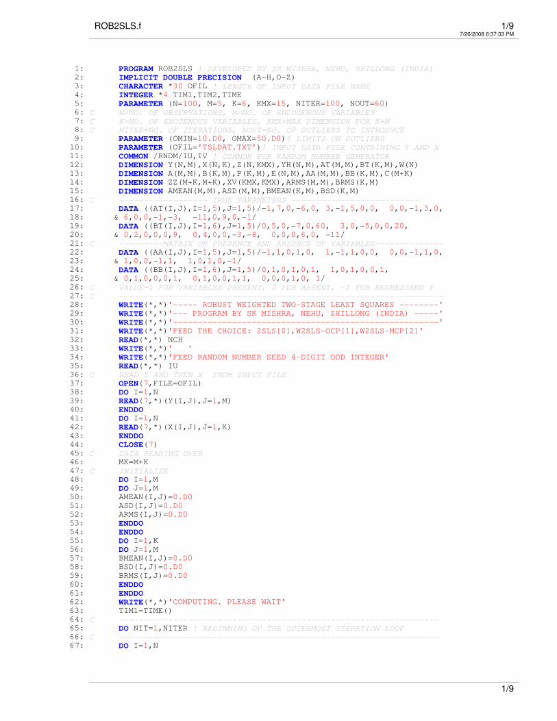
6. Conclusion: In this paper we have proposed a robust 2-Stage Weighted Least Squares
estimator for estimating the parameters of a multi-equation econometric model when data
contain outliers. The estimator is based on the procedure developed by Norm Campbell which
has been modified by using the measure of robust median deviation suggested by Hampel et al.
The estimation method based on the original Campbell procedure performs poorly, while the
method based on the modified Campbell procedure shows appreciable robustness. Robustness
of the proposed method is not much destabilized by the magnitude of outliers, but it is sensitive
to the number of outliers/perturbations in the data matrix. The breakdown point of the method,
is somewhere between 45 to 50 percent of the number of points in the data matrix.
References
• Campbell, N. A. (1980) “Robust Procedures in Multivariate Analysis I: Robust Covariance
Estimation”, Applied Statistics, 29 (3): 231-237
• Hampel, F. R., Ronchetti, E.M., Rousseeuw, P.J. and W. A. Stahel, W.A. (1986) Robust Statistics:
The Approach Based on Influence Functions, Wiley, New York.
• Mishra, S. K. (2008) “A New Method of Robust Linear Regression Analysis: Some Monte Carlo
Experiments”, Working Paper Series, SSRN at http://ssrn.com/abstract=1155135
GENDAT.f 1/37/26/2008 6:36:43 PM
1: PROGRAM GENDAT ! ------------------------------------------------2: PARAMETER (N=100,M=5,K=6,NCUE=1)
3: C N=NO. OF OBSERVATIONS, M=NO. OF EQUATIONS (= NO. OF ENDOGENOUS4: C VARIABLES, Y) AND K=NO. OF EXOGENOUS VARIABLES (X) INCLUDING A5: C UNITARY VARIABLE ASSOCIATED WITH THE INTERCEPT IN THE KTH COLUMN.6: C IF NCUE=1 THEN U WITH N(0,SDU) IS DIRECTLY GENERATED & ADDED TO Y7: C IF NCUE=0, U IS -E*INV(A), E WITH N(0,SDE). THEN U IS ADDED TO Y8: IMPLICIT DOUBLE PRECISION (A-H,O-Z)
9: PARAMETER (XLOW=0,XRANGE=20, SDU=0.0010D0,SDE=1.818D-07)
10: C XLOW=LOWEST LIMIT ON X(I,J); XRANGE=RANGE OF X(I,J) FROM XLOW TO11: C XHIGH, THE UPPER LIMIT OF X(I,J). SDU=STANDARD DEVIATION OF NORMAL12: C ERROR U WITH N(0, SDU), SDE OF E WITH N(0,SDE).13: CHARACTER *30 OFIL
14: PARAMETER (OFIL='TSLDAT.TXT')
15: COMMON /RNDM/IU,IV
16: DIMENSION Y(N,M),X(N,K),A(M,M),B(K,M),P(K,M),E(N,M),U(N,M)
17: C -------------- Structural Parameters -----------------------18: DATA ((A(I,J),I=1,5),J=1,5)/-1,7,0,-6,0, 3,-1,5,0,0, 0,0,-1,3,0,
19: & 6,0,0,-1,-3, -11,0,9,0,-1/
20: DATA ((B(I,J),I=1,6),J=1,5)/0,5,0,-7,0,60, 3,0,-5,0,0,20,
21: & 0,2,0,0,0,9, 0,4,0,0,-3,-8, 0,0,0,6,0, -11/
22: C -----------------------------------------------------------------23: WRITE(*,*)'FEED A 4-DIGIT ODD NON-ZERO RANDOM NUMBER SEED'
24: READ(*,*) IU
25: C PRINT TRANSPOSE(A) AND TRANSPOSE(B)26: C -----------------------------------------------------------------27: WRITE(*,*)'TRANSPOSED A MATRIX'
28: DO J=1,M
29: WRITE(*,10)(A(I,J),I=1,M)
30: ENDDO
31: WRITE(*,*)' '
32: WRITE(*,*)'TRANSPOSED B MATRIX'
33: DO J=1,M
34: WRITE(*,10)(B(I,J),I=1,K)
35: ENDDO
36: WRITE(*,*)' '
37: 10 FORMAT(6F7.0)
38: C -----------------------------------------------------------------39: C GENERATE X(N,K)40: DO I=1,N
41: DO J=1,K-1
42: CALL RANDOM(RAND)
43: X(I,J)=XLOW+RAND*XRANGE
44: ENDDO
45: ENDDO
46: DO I=1,N
47: X(I,K)=1.D0
48: ENDDO
49: C INVERT A MATRIX AND FIND P=-B*INV(A)50: CALL MINV(A,M,D)
51: WRITE(*,*)'DETERMINANT=',D
52: DO I=1,K
53: DO J=1,M
54: P(I,J)=0.D0
55: DO JJ=1,M
56: P(I,J)=P(I,J)+B(I,JJ)*A(JJ,J)
57: ENDDO
58: ENDDO
59: ENDDO
60: C PRINT P MATRIX61: WRITE(*,*)'REDUCED FORM COEEFIENTS OR P MATRIX ---------------'
62: DO I=1,K
63: WRITE(*,1)(P(I,J),J=1,M)
64: ENDDO
65: 1 FORMAT(6F12.4)
66: C OBTAIN Y= XP67: DO I=1,N
1/3

GENDAT.f 2/37/26/2008 6:36:43 PM
68: DO J=1,M
69: Y(I,J)=0.D0
70: DO JJ=1,K
71: Y(I,J)=Y(I,J)+X(I,JJ)*P(JJ,J)
72: ENDDO
73: ENDDO
74: ENDDO
75: C PRINT Y (WITHOUT ERROR)76: WRITE(*,*)'-------Y WITHOUT ERROR ------------------------------'
77: DO I=1,N
78: WRITE(*,1)(Y(I,J),J=1,M)
79: ENDDO
80: C --------------- ADDING U WITH N(0,SDU) TO Y DIRECTLY -----------81: IF(NCUE.EQ.1) THEN
82: C ADD NORMAL ERRORS TO Y83: DO J=1,M
84: DO I=1,N
85: CALL NORMAL(RAND) ! GENERATE NORMALLY DISTRIBUTED ERRORS N(0,SDE)86: Y(I,J)=Y(I,J)+RAND*SDU ! ADD ERROR TO Y87: ENDDO
88: ENDDO
89: ENDIF
90: C --- GENERATING U = -E INV(A) AND ADDING TO Y ------------------91: IF(NCUE.EQ.0) THEN
92: DO I=1,N
93: DO J=1,M
94: CALL NORMAL(RAND)
95: E(I,J)=RAND*SDE
96: ENDDO
97: ENDDO
98: DO I=1,N
99: DO J=1,M
100: U(I,J)=0.D0
101: DO JJ=1,M
102: U(I,J)=U(I,J)-E(I,JJ)*A(JJ,J)
103: ENDDO
104: ENDDO
105: ENDDO
106: DO I=1,N
107: DO J=1,M
108: Y(I,J)=Y(I,J)+U(I,J)
109: ENDDO
110: ENDDO
111: ENDIF
112: C -----------------------------------------------------------------113: C PRINT Y (WITH ERROR ADDED)114: WRITE(*,*)'-------Y WITH ERROR ------------------------------'
115: DO I=1,N
116: WRITE(*,1)(Y(I,J),J=1,M)
117: ENDDO
118: OPEN(7,FILE=OFIL)
119: DO I=1,N
120: WRITE(7,1)(Y(I,J),J=1,M)
121: ENDDO
122: DO I=1,N
123: WRITE(7,1)(X(I,J),J=1,K)
124: ENDDO
125: WRITE(7,*)'P MATRIX -------------------------------------------'
126: DO J=1,K
127: WRITE(7,1)(P(J,JJ),JJ=1,M)
128: ENDDO
129: CLOSE(7)
130: END
131: C -----------------------------------------------------------------132: C RANDOM NUMBER GENERATOR (UNIFORM BETWEEN 0 AND 1 - BOTH EXCLUSIVE)133: SUBROUTINE RANDOM(RAND)
134: IMPLICIT DOUBLE PRECISION (A-H,O-Z)
2/3

GENDAT.f 3/37/26/2008 6:36:43 PM
135: COMMON /RNDM/IU,IV
136: IV=IU*65539
137: IF(IV.LT.0) THEN
138: IV=IV+2147483647+1
139: ENDIF
140: RAND=IV
141: IU=IV
142: RAND=RAND*0.4656613E-09
143: RETURN
144: END
145: C -----------------------------------------------------------------146: SUBROUTINE NORMAL(R)
147: C PROGRAM TO GENERATE N(0,1) FROM RECTANGULAR RANDOM NUMBERS148: C IT USES VARIATE TRANSFORMATION FOR THIS PURPOSE.149: C -----------------------------------------------------------------150: C IF U1 AND U2 ARE UNIFORMLY DISTRIBUTED RANDOM NUMBERS (0,1),151: C THEN X=[(-2*LN(U1))**.5]*(COS(2*PI*U2) IS N(0,1)152: C PI = 4*ARCTAN(1.0)= 3.1415926535897932384626433832795153: C 2*PI = 6.283185307179586476925286766559154: C -----------------------------------------------------------------155: IMPLICIT DOUBLE PRECISION (A-H,O-Z)
156: COMMON /RNDM/IU,IV
157: C -----------------------------------------------------------------158: CALL RANDOM(RAND) ! INVOKES RANDOM TO GENERATE UNIFORM RAND [0, 1]159: U1=RAND ! U1 IS UNIFORMLY DISTRIBUTED [0, 1]160: CALL RANDOM(RAND) ! INVOKES RANDOM TO GENERATE UNIFORM RAND [0, 1]161: U2=RAND ! U1 IS UNIFORMLY DISTRIBUTED [0, 1]162: R=DSQRT(-2.D0*DLOG(U1))
163: R=R*DCOS(U2*6.283185307179586476925286766559D00)
164: C R=R*DCOS(U2*6.28318530718D00)165: RETURN
166: END
167: C -----------------------------------------------------------------168: C SUBROUTINE FOR MATRIX INVERSION169: SUBROUTINE MINV(A,N,D)
170: IMPLICIT DOUBLE PRECISION (A-H,O-Z)
171: DIMENSION A(N,N)
172: U=1.D0
173: D=U
174: DO I=1,N
175: D=D*A(I,I)
176: A(I,I)=U/A(I,I)
177: DO J=1,N
178: IF(I.NE.J) A(J,I)=A(J,I)*A(I,I)
179: ENDDO
180: DO J=1,N
181: DO K=1,N
182: IF(I.NE.J.AND.K.NE.I) A(J,K)=A(J,K)-A(J,I)*A(I,K)
183: ENDDO
184: ENDDO
185: DO J=1,N
186: IF(J.NE.I) A(I,J)= -A(I,J)*A(I,I)
187: ENDDO
188: ENDDO
189: RETURN
190: END
3/3
ROB2SLS.f 1/97/26/2008 6:37:33 PM
1: PROGRAM ROB2SLS ! DEVELOPED BY SK MISHRA, NEHU, SHILLONG (INDIA)2: IMPLICIT DOUBLE PRECISION (A-H,O-Z)
3: CHARACTER *30 OFIL ! LENGTH OF INPUT DATA FILE NAME4: INTEGER *4 TIM1,TIM2,TIME
5: PARAMETER (N=100, M=5, K=6, KMX=15, NITER=100, NOUT=60)
6: C N=NO. OF OBSERVATIONS, M=NO. OF ENDOGENOUS VARIABLES7: C K=NO. OF EXOGENOUS VARIABLES, KMX=MAX DIMENSION FOR K+M8: C NITER=NO. OF ITERATIONS, NOUT=NO. OF OUTLIERS TO INTRODUCE9: PARAMETER (OMIN=10.D0, OMAX=50.D0)! LIMITS ON OUTLIERS10: PARAMETER (OFIL='TSLDAT.TXT')! INPUT DATA FILE CONTAINING Y AND X11: COMMON /RNDM/IU,IV ! COMMON FOR RANDOM NUMBER GENERATOR12: DIMENSION Y(N,M),X(N,K),Z(N,KMX),YH(N,M),AT(M,M),BT(K,M),W(N)
13: DIMENSION A(M,M),B(K,M),P(K,M),E(N,M),AA(M,M),BB(K,M),C(M+K)
14: DIMENSION ZZ(M+K,M+K),XV(KMX,KMX),ARMS(M,M),BRMS(K,M)
15: DIMENSION AMEAN(M,M),ASD(M,M),BMEAN(K,M),BSD(K,M)
16: C ------------------ TRUE PARAMETERS --------------------------17: DATA ((AT(I,J),I=1,5),J=1,5)/-1,7,0,-6,0, 3,-1,5,0,0, 0,0,-1,3,0,
18: & 6,0,0,-1,-3, -11,0,9,0,-1/
19: DATA ((BT(I,J),I=1,6),J=1,5)/0,5,0,-7,0,60, 3,0,-5,0,0,20,
20: & 0,2,0,0,0,9, 0,4,0,0,-3,-8, 0,0,0,6,0, -11/
21: C ---------MATRIX OF PRESENCE AND ABSENCE OF VARIABLES--------------22: DATA ((AA(I,J),I=1,5),J=1,5)/-1,1,0,1,0, 1,-1,1,0,0, 0,0,-1,1,0,
23: & 1,0,0,-1,1, 1,0,1,0,-1/
24: DATA ((BB(I,J),I=1,6),J=1,5)/0,1,0,1,0,1, 1,0,1,0,0,1,
25: & 0,1,0,0,0,1, 0,1,0,0,1,1, 0,0,0,1,0, 1/
26: C VALUE=1 FOR VARIABLES PRESENT, 0 FOR ABSENT, -1 FOR REGRESSAND Y27: C ------------------------------------------------------------------28: WRITE(*,*)'----- ROBUST WEIGHTED TWO-STAGE LEAST SQUARES --------'
29: WRITE(*,*)'--- PROGRAM BY SK MISHRA, NEHU, SHILLONG (INDIA) -----'
30: WRITE(*,*)'------------------------------------------------------'
31: WRITE(*,*)'FEED THE CHOICE: 2SLS[0],W2SLS-OCP[1],W2SLS-MCP[2]'
32: READ(*,*) NCH
33: WRITE(*,*)' '
34: WRITE(*,*)'FEED RANDOM NUMBER SEED 4-DIGIT ODD INTEGER'
35: READ(*,*) IU
36: C READ Y AND THEN X FROM INPUT FILE37: OPEN(7,FILE=OFIL)
38: DO I=1,N
39: READ(7,*)(Y(I,J),J=1,M)
40: ENDDO
41: DO I=1,N
42: READ(7,*)(X(I,J),J=1,K)
43: ENDDO
44: CLOSE(7)
45: C DATA READING OVER46: MK=M+K
47: C INITIALIZE48: DO I=1,M
49: DO J=1,M
50: AMEAN(I,J)=0.D0
51: ASD(I,J)=0.D0
52: ARMS(I,J)=0.D0
53: ENDDO
54: ENDDO
55: DO I=1,K
56: DO J=1,M
57: BMEAN(I,J)=0.D0
58: BSD(I,J)=0.D0
59: BRMS(I,J)=0.D0
60: ENDDO
61: ENDDO
62: WRITE(*,*)'COMPUTING. PLEASE WAIT'
63: TIM1=TIME()
64: C -----------------------------------------------------------------65: DO NIT=1,NITER ! BEGINNING OF THE OUTERMOST ITERATION LOOP66: C -----------------------------------------------------------------67: DO I=1,N
1/9
ROB2SLS.f 2/97/26/2008 6:37:33 PM
68: DO J=1,M
69: Z(I,J)=Y(I,J)
70: ENDDO
71: DO J=1,K
72: Z(I,M+J)=X(I,J)
73: ENDDO
74: ENDDO
75: C ADD NOUT NUMBER OF OUTLIERS AT RANDOM LOCATIONS76: IF(NOUT.EQ.0) THEN
77: NOUTLIER=1
78: MULT=0
79: ELSE
80: NOUTLIER=NOUT
81: MULT=1
82: ENDIF
83: DO I=1,NOUTLIER
84: CALL OUTLIER(N,M,OMIN,OMAX,IX,JX,OL)
85: Z(IX,JX)=Z(IX,JX)+OL*MULT
86: ENDDO
87: C ASSIGNMENT OF WEIGHTS -------------------------------------------88: DO I=1,N
89: W(I)=1.D0
90: ENDDO
91: IF(NCH.EQ.1) CALL RCAMPBELL(Z,N,MK,W)
92: IF(NCH.EQ.2) CALL MCAMPBELL(Z,N,MK,W)
93: C -----------------------------------------------------------------94: C COMPUTE Z'Z95: DO J=1,MK
96: DO JJ=1,MK
97: ZZ(J,JJ)=0.D0
98: DO I=1,N
99: ZZ(J,JJ)=ZZ(J,JJ)+Z(I,J)*Z(I,JJ)*W(I)**2
100: ENDDO
101: ENDDO
102: ENDDO
103: C STORE X'X INTO XV104: DO J=1,K
105: DO JJ=1,K
106: XV(J,JJ)=ZZ(M+J,M+JJ)
107: ENDDO
108: ENDDO
109: C WRITE(*,*)'XV MATRIX'110: C DO J=1,K111: C WRITE(*,1)(XV(J,JJ),JJ=1,K)112: C ENDDO113: C INVERT XX114: CALL MINV(XV,K,D)
115: C PRE-MULTIPLY INVERTED XV BY X'Y116: C WRITE(*,*)'INVERTED MATRIX DET =',D117: C DO J=1,K118: C WRITE(*,2)(XV(J,JJ),JJ=1,K)119: C ENDDO120: DO J=1,K
121: DO JJ=1,M
122: P(J,JJ)=0.D0
123: DO I=1,K
124: P(J,JJ)=P(J,JJ)+XV(J,I)*ZZ(I+M,JJ)
125: ENDDO
126: ENDDO
127: ENDDO
128: C PRING COMPUTED P MATRIX129: C WRITE(*,*)'ESTIMATED P MATRIX'130: C DO I=1,K131: C WRITE(*,1)(P(I,J),J=1,M)132: C ENDDO133: 1 FORMAT(6F12.4)
134: 2 FORMAT(6E12.5)
2/9

ROB2SLS.f 3/97/26/2008 6:37:33 PM
135: C COMPUTE ESTIMATED Y; YH=XP136: DO I=1,N
137: DO J=1,M
138: YH(I,J)=0.D0
139: DO JJ=1,K
140: YH(I,J)=YH(I,J)+X(I,JJ)*P(JJ,J)
141: ENDDO
142: ENDDO
143: ENDDO
144: C SECOND STAGE OF 2-STAGE LEAST SQUARES145: DO J=1,M ! FOR M EQUATIONS146: DO I=1,N
147: Z(I,1)=Y(I,J)
148: ENDDO
149: J1=0
150: DO JJ=1,M
151: IF(AA(JJ,J).GT.0) THEN
152: J1=J1+1
153: DO I=1,N
154: Z(I,J1+1)=YH(I,JJ)
155: ENDDO
156: ENDIF
157: ENDDO
158: DO JJ=1,K
159: IF(BB(JJ,J).GT.0) THEN
160: J1=J1+1
161: DO I=1,N
162: Z(I,J1+1)=(-X(I,JJ))
163: C ! ------ (-X DUE TO CHANGE IN SIGN OF Y)164: ENDDO
165: ENDIF
166: ENDDO
167: J2=J1+1
168: IF(NCH.EQ.1) CALL RCAMPBELL(Z,N,J2,W)
169: IF(NCH.EQ.2) CALL MCAMPBELL(Z,N,J2,W)
170: DO JA=1,J2
171: DO JB=1,J2
172: ZZ(JA,JB)=0.D0
173: DO I=1,N
174: ZZ(JA,JB)=ZZ(JA,JB)+Z(I,JA)*Z(I,JB)*W(I)**2
175: ENDDO
176: ENDDO
177: ENDDO
178: DO JA=1,J1
179: DO JB=1,J1
180: XV(JA,JB)=ZZ(JA+1,JB+1)
181: ENDDO
182: ENDDO
183: CALL MINV(XV,J1,D)
184: DO JA=1,J1
185: C(JA)=0.D0
186: DO JB=1,J1
187: C(JA)=C(JA)+XV(JA,JB)*ZZ(JB+1,1)
188: ENDDO
189: ENDDO
190: C WRITE(*,*)'EQUATION NUMBER =', J191: C WRITE(*,1)(C(JA),JA=1,J1)192: C PLACE COEFFICIENTS IN PROPER MATRIX CELL193: J1=0
194: DO JA=1,M
195: IF(AA(JA,J).GT.0) THEN
196: J1=J1+1
197: A(JA,J)=C(J1)
198: ELSE
199: IF(JA.EQ.J) A(JA,J)=-1
200: ENDIF
201: ENDDO
3/9

ROB2SLS.f 4/97/26/2008 6:37:33 PM
202: DO JA=1,K
203: IF(BB(JA,J).GT.0) THEN
204: J1=J1+1
205: B(JA,J)=C(J1)
206: ENDIF
207: ENDDO
208: C WRITE(*,*)'EQUATION NUMBER =', J209: C WRITE(*,1)(A(JA,J),JA=1,M)210: C WRITE(*,1)(B(JA,J),JA=1,K)211: ENDDO
212: C ------------------------------------------------------------------213: DO I=1,M
214: DO J=1,M
215: AMEAN(I,J)=AMEAN(I,J)+A(I,J)
216: ASD(I,J)=ASD(I,J)+A(I,J)**2
217: ARMS(I,J)=ARMS(I,J)+(A(I,J)-AT(I,J))**2
218: ENDDO
219: ENDDO
220: DO I=1,K
221: DO J=1,M
222: BMEAN(I,J)=BMEAN(I,J)+B(I,J)
223: BSD(I,J)=BSD(I,J)+B(I,J)**2
224: BRMS(I,J)=BRMS(I,J)+(B(I,J)-BT(I,J))**2
225: ENDDO
226: ENDDO
227: ENDDO ! END OF THE OUTERMOST ITERATION LOOP228: WRITE(*,*)' '
229: WRITE(*,*)'----------- RESULTS OF MONTE CARLO EXPERIMENT --------'
230:
231: WRITE(*,*)' '
232: WRITE(*,*)'MEAN OF TRANSPOSE(A) COEFFICIENTS'
233: DO J=1,M
234: WRITE(*,1)(AMEAN(I,J)/NITER,I=1,M)
235: ENDDO
236: WRITE(*,*)'SD OF TRANSPOSE(A) COEFFICIENTS'
237: DO J=1,M
238: WRITE(*,1)(DSQRT(ASD(I,J)/NITER-(AMEAN(I,J)/NITER)**2),I=1,M)
239: ENDDO
240: WRITE(*,*)'RMS OF TRANSPOSE(A) COEFFICIENTS'
241: DO J=1,M
242: WRITE(*,1)(DSQRT(ARMS(I,J)/NITER),I=1,M)
243: ENDDO
244: WRITE(*,*)' '
245: WRITE(*,*)'MEAN OF TRANSPOSE(B) COEFFICIENTS'
246: DO J=1,M
247: WRITE(*,1)(BMEAN(I,J)/NITER,I=1,K)
248: ENDDO
249: WRITE(*,*)'SD OF TRANSPOSE(B) COEFFICIENTS'
250: DO J=1,M
251: WRITE(*,1)(DSQRT(BSD(I,J)/NITER-(BMEAN(I,J)/NITER)**2),I=1,K)
252: ENDDO
253: WRITE(*,*)'RMS OF TRANSPOSE(B) COEFFICIENTS'
254: DO J=1,M
255: WRITE(*,1)(DSQRT(BRMS(I,J)/NITER),I=1,K)
256: ENDDO
257: WRITE(*,*)' '
258: TIM2=TIME()
259: WRITE(*,*)'END OF THE EXPERIMENT. TIME TAKEN(SECONDS)=',TIM2-TIM1
260: END
261: C -----------------------------------------------------------------262: SUBROUTINE MEDIAN(X,N,A,V) ! ------------------------------------263: C SUBROUTINE MEDIAN : FINDS MEDIAN (A) AND MEAN DEVIATION (V) OF A264: C GIVEN VARIATE, VARIATE X(N)265: PARAMETER (NMAX=100)
266: IMPLICIT DOUBLE PRECISION (A-H,O-Z)
267: DIMENSION X(N),Z(NMAX)
268: C STORE X IN Z
4/9

ROB2SLS.f 5/97/26/2008 6:37:33 PM
269: DO I=1,N
270: Z(I)=X(I)
271: ENDDO
272: C ARRANGE Z IN AN ASCENDING ORDER273: DO I=1,N-1
274: DO J=I+1,N
275: IF(Z(I).GT.Z(J)) THEN ! EXCHANGE276: TEMP=Z(I)
277: Z(I)=Z(J)
278: Z(J)=TEMP
279: ENDIF
280: ENDDO
281: ENDDO
282: K=(N+1)/2 ! K IS OBTAINED AS INT((N+1)/2.0D0)283: A=(Z(K)+Z(N+1-K))/2.D0 ! GIVES MEDIAN FOR ODD AS WELL AS EVEN N284: C FIND MEAN DEVIATION285: V=0.D0
286: DO I=1,N
287: V=V+DABS(Z(I)-A) ! A IS MEDIAN288: ENDDO
289: V=V/N ! V IS MEAN DEVIATION FROM MEDIAN290: C WRITE(*,*)'MEDIAN =',A,' MEAN DEVIATION =',V291: RETURN
292: END
293: C ------------------------------------------------------------------294: C CAMPBELL COVARIANCE MATRIX (TYPE-I)295: SUBROUTINE RCAMPBELL(Z,N,MM,W)
296: PARAMETER(NV=100,MV=15,ITRN=200)
297: IMPLICIT DOUBLE PRECISION (A-H,O-Z)
298: DIMENSION X(NV,MV),V(MV,MV),AV(MV),W(NV),XD(MV)
299: DIMENSION D(NV),VV(MV,MV),DN(NV),Z(NV,MV)
300: DATA B1,B2/2, 1.5/
301: C SOME DEFINITIONS302: D0=DSQRT(DFLOAT(M))+B1/DSQRT(2.D0)
303: B22=B2**2
304: M=MM-1
305: DO I=1,N
306: DO J=1,M
307: X(I,J)=Z(I,J)
308: ENDDO
309: ENDDO
310: NSKIP=1
311: IF(NSKIP.NE.1) THEN ! DO NOT STANDARDIZE THE VARIABLES312: C STANDARDIZE313: DO J=1,M
314: AV(J)=0.D0
315: XD(J)=0.D0
316: DO I=1,N
317: AV(J)=AV(J)+X(I,J)
318: XD(J)=XD(J)+X(I,J)**2
319: ENDDO
320: AV(J)=AV(J)/N
321: XD(J)=DSQRT(XD(J)/N-AV(J)**2)
322: ENDDO
323: DO J=1,M
324: DO I=1,N
325: X(I,J)=(X(I,J)-AV(J))/XD(J)
326: ENDDO
327: ENDDO
328: ENDIF
329: C INITIALIZE WEIGHT VECTOR BY UNITY330: DO I=1,N
331: W(I)=1.D0
332: ENDDO
333: C FIND SUM OF WEIGHTS334: DO ITER=1,ITRN
335: SW=0.D0
5/9

ROB2SLS.f 6/97/26/2008 6:37:33 PM
336: SSW=0.D0
337: DO I=1,N
338: SW=SW+W(I)
339: SSW=SSW+W(I)**2
340: ENDDO
341: SSW=SSW-1.D0
342: C COMPUTE MEAN VECTOR AND COVARIANCE MATRIX343: DO J=1,M
344: AV(J)=0.D0
345: DO I=1,N
346: AV(J)=AV(J)+X(I,J)*W(I)
347: ENDDO
348: AV(J)=AV(J)/SW
349: ENDDO
350: DO J=1,M
351: DO JJ=J,M
352: V(J,JJ)=0.D0
353: DO I=1,N
354: V(J,JJ)=V(J,JJ)+(X(I,J)-AV(J))*(X(I,JJ)-AV(JJ))*W(I)**2
355: ENDDO
356: V(J,JJ)=V(J,JJ)/SSW
357: IF(J.NE.JJ) V(JJ,J)=V(J,JJ)
358: ENDDO
359: ENDDO
360: DO J=1,M
361: DO JJ=1,M
362: VV(J,JJ)=V(J,JJ)
363: ENDDO
364: ENDDO
365: C INVERT V366: CALL MINV(V,M,DD) ! ON RETURN V IS INVERTED V367: DO I=1,N
368: D(I)=0.D0
369: DO J=1,M
370: XD(J)=0.D0
371: DO JJ=1,M
372: XD(J)=XD(J)+(X(I,JJ)-AV(JJ))*V(JJ,J)
373: ENDDO
374: ENDDO
375: DD=0.D0
376: DO J=1,M
377: DD=DD+XD(J)*(X(I,J)-AV(J))
378: ENDDO
379: D(I)=DD
380: DN(I)=DD
381: ENDDO
382: DO I=1,N
383: IF(D(I).LE.D0)THEN
384: WD= D(I)
385: ELSE
386: WD=D0*DEXP(-0.5D0*(D(I)-D0)**2/B22)
387: ENDIF
388: W(I)=1.D0
389: IF(DABS(D(I)).GT.1.0D-05) W(I)=WD/D(I)
390: ENDDO
391: ENDDO
392: DO J=1,M
393: DO JJ=1,M
394: V(J,JJ)=VV(J,JJ)
395: ENDDO
396: ENDDO
397: C DO J=1,M398: C WRITE(*,1)(V(J,JJ),JJ=1,M)399: C ENDDO400: 1 FORMAT(10F7.3)
401: C WRITE(*,*)'------------------------------------------------------'402: C WEIGTING Z MATRIX
6/9

ROB2SLS.f 7/97/26/2008 6:37:33 PM
403: DO J=1,MM
404: DO I=1,N
405: Z(I,J)=Z(I,J)*W(I)
406: ENDDO
407: ENDDO
408: RETURN
409: END
410: C ------------------------------------------------------------------411: C CAMPBELL COVARIANCE MATRIX (TYPE-II)412: SUBROUTINE MCAMPBELL(Z,N,MM,W)
413: PARAMETER(NV=100,MV=15,ITRN=200)
414: IMPLICIT DOUBLE PRECISION (A-H,O-Z)
415: DIMENSION X(NV,MV),V(MV,MV),AV(MV),W(NV),XD(MV)
416: DIMENSION D(NV),VV(MV,MV),DN(NV),Z(NV,MV)
417: M=MM-1
418: DO I=1,N
419: DO J=1,M
420: X(I,J)=Z(I,J)
421: ENDDO
422: ENDDO
423: NSKIP=1
424: IF(NSKIP.NE.1) THEN ! DO NOT STANDARDIZE THE VARIABLES425: C STANDARDIZE426: DO J=1,M
427: AV(J)=0.D0
428: XD(J)=0.D0
429: DO I=1,N
430: AV(J)=AV(J)+X(I,J)
431: XD(J)=XD(J)+X(I,J)**2
432: ENDDO
433: AV(J)=AV(J)/N
434: XD(J)=DSQRT(XD(J)/N-AV(J)**2)
435: ENDDO
436: DO J=1,M
437: DO I=1,N
438: X(I,J)=(X(I,J)-AV(J))/XD(J)
439: ENDDO
440: ENDDO
441: ENDIF
442: C INITIALIZE WEIGHT VECTOR BY UNITY443: DO I=1,N
444: W(I)=1.D0
445: ENDDO
446: C FIND SUM OF WEIGHTS447: DO ITER=1,ITRN
448: SW=0.D0
449: SSW=0.D0
450: DO I=1,N
451: SW=SW+W(I)
452: SSW=SSW+W(I)**2
453: ENDDO
454: SSW=SSW-1.D0
455: C COMPUTE MEAN VECTOR AND COVARIANCE MATRIX456: DO J=1,M
457: AV(J)=0.D0
458: DO I=1,N
459: AV(J)=AV(J)+X(I,J)*W(I)
460: ENDDO
461: AV(J)=AV(J)/SW
462: ENDDO
463: DO J=1,M
464: DO JJ=J,M
465: V(J,JJ)=0.D0
466: DO I=1,N
467: V(J,JJ)=V(J,JJ)+(X(I,J)-AV(J))*(X(I,JJ)-AV(JJ))*W(I)**2
468: ENDDO
469: V(J,JJ)=V(J,JJ)/SSW
7/9

ROB2SLS.f 8/97/26/2008 6:37:33 PM
470: IF(J.NE.JJ) V(JJ,J)=V(J,JJ)
471: ENDDO
472: ENDDO
473: DO J=1,M
474: DO JJ=1,M
475: VV(J,JJ)=V(J,JJ)
476: ENDDO
477: ENDDO
478: C INVERT V479: CALL MINV(V,M,DD) ! ON RETURN V IS INVERTED V480: DO I=1,N
481: D(I)=0.D0
482:
483: DO J=1,M
484: XD(J)=0.D0
485: DO JJ=1,M
486: XD(J)=XD(J)+(X(I,JJ)-AV(JJ))*V(JJ,J)
487: ENDDO
488: ENDDO
489: DD=0.D0
490: DO J=1,M
491: DD=DD+XD(J)*(X(I,J)-AV(J))
492: ENDDO
493: D(I)=DD
494: DN(I)=DD
495: ENDDO
496: CALL MEDIAN(DN,N,DNA,DNV)
497: DO I=1,N
498: DN(I)=DABS(DN(I)-DNA)
499: ENDDO
500: CALL MEDIAN(DN,N,DNAA,DNVV)
501: DNAA=DNAA/0.6745D0
502: DO I=1,N
503: W(I)=0.D0
504: DX=DABS(D(I)-DNA)
505: IF(DX.LE.DNAA) W(I)=1.D0
506: IF(DX.LE.2*DNAA.AND.DX.GT.DNAA) W(I)=.25D0
507: IF(DX.LE.3*DNAA.AND.DX.GT.2*DNAA) W(I)=0.1111111111D0
508: IF(DX.LE.4*DNAA.AND.DX.GT.3*DNAA) W(I)=0.0625D0
509: ENDDO
510: ENDDO
511: DO J=1,M
512: DO JJ=1,M
513: V(J,JJ)=VV(J,JJ)
514: ENDDO
515: ENDDO
516: C DO J=1,M517: C WRITE(*,1)(V(J,JJ),JJ=1,M)518: C ENDDO519: 1 FORMAT(10F7.3)
520: C WRITE(*,*)'------------------------------------------------------'521: C WEIGHTING Z MATRIX522: DO J=1,MM
523: DO I=1,N
524: Z(I,J)=Z(I,J)*W(I)
525: ENDDO
526: ENDDO
527: RETURN
528: END
529: C -----------------------------------------------------------------530: C SUBROUTINE FOR MATRIX INVERSION531: SUBROUTINE MINV(A,N,D)
532: PARAMETER(KMX=15)! MUST BE CONSISTEN WITH KMX IN THE MAIN PROGRAM533: IMPLICIT DOUBLE PRECISION (A-H,O-Z)
534: DIMENSION A(KMX,KMX)
535: U=1.D0
536: D=U
8/9

ROB2SLS.f 9/97/26/2008 6:37:33 PM
537: DO I=1,N
538: D=D*A(I,I)
539: A(I,I)=U/A(I,I)
540: DO J=1,N
541: IF(I.NE.J) A(J,I)=A(J,I)*A(I,I)
542: ENDDO
543: DO J=1,N
544: DO K=1,N
545: IF(I.NE.J.AND.K.NE.I) A(J,K)=A(J,K)-A(J,I)*A(I,K)
546: ENDDO
547: ENDDO
548: DO J=1,N
549: IF(J.NE.I) A(I,J)= -A(I,J)*A(I,I)
550: ENDDO
551: ENDDO
552: RETURN
553: END
554: C -----------------------------------------------------------------555: C RANDOM NUMBER GENERATOR (UNIFORM BETWEEN 0 AND 1 - BOTH EXCLUSIVE)556: SUBROUTINE RANDOM(RAND)
557: IMPLICIT DOUBLE PRECISION (A-H,O-Z)
558: COMMON /RNDM/IU,IV
559: IV=IU*65539
560: IF(IV.LT.0) THEN
561: IV=IV+2147483647+1
562: ENDIF
563: RAND=IV
564: IU=IV
565: RAND=RAND*0.4656613E-09
566: RETURN
567: END
568: C -----------------------------------------------------------------569: SUBROUTINE OUTLIER(N,M,OMIN,OMAX,IX,JX,OL)
570: IMPLICIT DOUBLE PRECISION (A-H,O-Z)
571: COMMON /RNDM/IU,IV
572: 1 CALL RANDOM(RAND)
573: KK=INT(RAND*N*M)+1
574: JX=MOD(KK,M)
575: IF(JX.EQ.0) GOTO 1
576: IX=KK/M+1
577: CALL RANDOM(RAND)
578: OL=OMIN+(OMAX-OMIN)*(RAND-0.5D0)
579: C OL IS THE SIZE (quantum) OF PERTURBATION AND IX AND JX POINT580: C TO THE LOCATION WHERE OL WOULD BE ADDED TO DATA, Z.581: RETURN
582: END
583:
9/9