Fuzzy Least Squares

INFORMATION SCIENCES 46,141-157 (1988) 141

F-Yh=tsqu-

PHIL DIAMOND*

Centre de Ghstaiistique, ENSMP, Fontainebleay France

ABSTRACT

Several models for simple least-squares fitting of fuzzy-valued data are developed. Criteria are given for when fuzzy data sets can be fitted to the models, and analogues of the normal

equations are derived.

INTRODUCTION

Most modeling techniques, control problems, and operations-research algorithms are designed for manipulating exact numerical data, or data which are uncertain in some well-defined statistical sense. Moore [6] has suggested not only that the first approach might often be unrealistic, but also that it could frequently obscure some aspects of structural behavior, and has advocated the use of interval analysis as a conjoint. On the other hand, stochastic models may not be appropriate because necessary information is simply unavailable, or is very imprecise or even couched in terms that are not truly numerical. Fuzzy set theory has been regarded as a natural way of describing data of this type [l, 3, 7, 12, 131.

The commonest approach to fuzzy data appears to consist in the adaptation of existing algorithms by the extension principle, as in Prade [8] and Zimmerman [14], or of using fuzzy arithmetic on models already developed from nonfuzzy data. Yager [ll] and Hammerbacher and Yager [4] handled this last aspect by substituting fuzzy values into regression equations formulated from previous crisp data. Little seems to have been done in actually using the available fuzzy data themselves to determine fuzzy parameters, although [ll] hints at the possibility. Tanaka et al. [lo] used linear programming techniques to develop a model superficially resembling linear regression, but it is unclear

*Permanent address: Mathematics Department, University of Queen&nd, Brisbane Qld, 4067 Australia.

Wlsevier Science Publishing Co., Inc. 1988 655 Avenue of the Ame&as, New York, NY 10010 0020-0255/88/$03.50

142 PHIL DIAMOND

what the relation is to a least-squares concept, or that any measure of best fit by residuals is present. If genuinely fuzzy algorithms are to use fuzzy initial conditions, and are to incorporate fuzzy parameters estimated from existing data, it is of some importance to measure how accurately these reflect the

prevailing fuzziness. This note addresses part of this problem. Several models are proposed as

fuzzy analogues of simple linear least squares, and use fuzzy data to compute

the parameters. Criteria are developed for the classes of fuzzy data which can

be meaningfully processed using this approach. Equations are derived which are rather similar to the normal equations of classic least squares. Data will be

restricted to triangular fuzzy numbers, but the severity of this condition is more than compensated for by the resulting computational simplicity.

MATHEMATICAL PRELIMINARIES

Let 9(R) denote the set of normalized fuzzy numbers: that is, the set of upper semicontinuous convex functions X: R + [0, l] such that

{UER: X(24)=1} is nonempty. Denote by 2$(R) the set of fuzzy numbers

with compact cw-levels X,, for each a > 0. A metric d* can be defined on q(R)

byd*(X,Y)=sw,>, ,, d (X,, Y,), where the Hausdorff metric dH is given as

The metric space (S$( R), d*) is complete [9]. Suppose that L, R are even, nonincreasing real functions on [0, co), satisfy-

ing L(0) = R(0) =l. Fuzzy numbers of the form

i

for x<m, a>O,

X(u) = for x>m, b>O,

(1)

have proved extremely useful. For given functions L and R, (1) is called an L, R-representation and denoted X= (m, a, b),,, where m is the modal value of X and u, b the left and right spreads respectively [2,3]. A linear structure can be defined on L, R-fuzzy numbers by (m, a, b),, + (m’, a’, b’),, = (m + m’, a + a’, b + b?,,, t(m, a, b),, = (tm, ta, tb),, if t > 0, t(m, a, b),,

FUZZY LEAST SQUARES 143

= (fm, tb, la),, if t < 0. If L, R are of the form

then X- (m, a, b)T is said to be triangular. Let Y(R) denote the set of triangular fuzzy numbers (m, a, b)=.

To digress briefly: the space of nonempty compact convex subsets of R” can be embedded in a Banach space by identification with support functions. For such a set A c R”, define

s(X,A) =su~((XJ}:AW’-~, x=A).

Here (,) is the usual inner product in R”, and .67-l the (n - l)-sphere in R”. The continuous function h * s(X, A) completely determines A (151. It is now possible to define an b-metric

For compact intervals, the metric Dr takes au especially simple form because the support function is defined at just two points, - 1 and -t- 1. If A = [_A, x], B=fB,Zj], thell

This is an equivalent metric to dH on the space of compact intervals. For X, Y E J(R) define

where supp X denotes the compact interval of support of X, and m(X) its modal vahre. Clearly (r(R), d) is complete. If X = (x, {, g),, Y = ( y, 2, y)r, then

Let B(R) be that subspace of y(R) all of whose elements have nonnegative support: that is, for each (m, a, b)T, m - a > 0. Then 8(R) is a cone in

144 PHIL DIAMOND

9(R) and is a closed convex subset of r(R) with respect to the topology induced by d.

EXISTENCE OF MINIMIZING FUZZY NUMBERS

Let Y be a cone in 9(R), and let X= (x, 5, {), E 9(R). Write elements of Y as V= (u,_w,i& The supports of X,V are-closedintervals [_X, %],[_V,v]. If

there exists a fuzzy number V, E Y such that for every V in V

then X is said to be V,-orthogonal to Y.

THEOREM 1. Let -Y be a closed cone in 9(R). For any X in 9(R) there is a unique triangular fuzzy number V, in Y such that d( X, V,) G d( X, V) for all V in VT. A necessary and sufficient condition for V, to be the unique minimizing fwzy number in Y is that X is VO-orthogonal to Y.

Two lemmas facilitate the proof of Theorem 1.

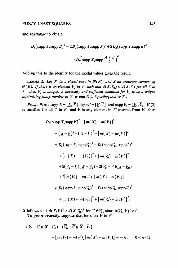
LEMMAS. d(A,B)*=2d(A,X)*+2d(X,B)*-4d(X,(A+B)/2)*.

Proof.

2[m(A)-m(X)]*+2[m(X)-m(B)]*

= {[m(A)-m(X)l+[m(X)-m(B)l}*

by the usual parallelogram law calculation. Moreover, 2(_F* + F*) + 2(_G2+~2)=(_F-_G)2+(~-G)2+(_F+G)2+(~+~)2. Let A= (m(A), cll, G, B=(m(B),L%&, X=(m(X),$,&; put F=~(A)-cz- [m(X)-$1, G=m(X)-$zim(B)-_81,

?=m(A)+Z-[m(X)+g], G=m(X)+g-[m(B)+B];


and rearrange to obtain

.

Adding this to the identity for the modal values gives the result.

LEMMA 2. L-et V be a closed cone in 9(R), and X an arbitra? element of 9(R). If there is an element V, in Y such that d( X, V,) < d( X, V) for all V in V, then V, is unique. A necessary and sufficient condition for V, to be a unique minimizing fuzzy number in Y is that X is VO-orthogonal to Y.

Proof. Write suppX= [_X, k], suppV= [_V,v], and suppV, = [IO,%]. If (3) is satisfied for all V in Y, and V is any element in Y distinct from V,, then

+[m(X)-m(V,)12+[m(VO)--m(V)12

+qKl -!!>(_x-KI) +q 6 - q(x-_voo)

+2[m(V,)-m(V)l[m(X)-m(~‘,)l

It follows that d( X, V)2 > d( X, V,)2 for V# V,, since d(&, V)2 > 0. To prove necessity, suppose that for some V in Y

<_v,-_v)(_x--v,)+(v,-V)(X-v,)

+[m(v,)-m(V>l[m(X)-m(~‘,)] =-A, O<h<l.

146

Without loss of generality, suppose + XV, which is in Y by convexity:

PHIL DIAMOND

that d(V,G)=l. Consider 6-(1-A)&

and V, is not a minimizing element on Y.

Proof of Theorem 1. Uniqueness and the sufficiency of I$-orthogonality follow from Lemma 2. It remains to show the existence of V,. If X is in Y there is nothing to prove. So assume X is not in Y, and define S = inf{ df X, V) : V E Y}. Let v be a sequence of fuzzy numbers in V such that d(X,y)+& ByLemmal,

d(&y)2=2d(&,X)2+26(X,q)2-4d X ( ,qq’.

For all i, j, (y + I$)/2 is in Ilr because the cone Y is convex. Thus d( X, (y + 5)/2) 2 6 and d(& 5)” G Zd(q, X)2 + 2d( X, 5)” - 4S2, so d( 5, I$) + 0 as i, j + 00. So (&} is a Cauchy sequence, and since F(R) is complete and Y closed, V, = lim F is in 7v.

COROLLARY 1. Let N be a positive integer, and suppose that Y is a closed cone in zF(R)~. Denote by dhr the metric on LS’(R)~ deemed by

d,(v,W)2= : d(WK)2, V,WE~‘(R)~, i-l

where K,H$EE(R), i=l,..., N, are the components of V, W. Then for any X in .f3r( R)N there is a unique N-vector V, in Y such that dN( X, V,) Q dN( X, V) for aI/ V in Y.

Proof. The parahelogram-like law of Lemma 1 extends to d,, so the existence of V, follows in the theorem. Uniqueness comes from a similar argument to that of Lemma 2.


FUZZY INPUT, FUZZY OUTPUT

Suppose that observations consist of data pairs X,, y, i = 1,2,. . . , N, where X,(x;,&,&&, q=(_y,,~~,j~)r. It is assumed throughout that xi-&>O, by a simple translation of all data if necessary, and that X is the explanatory variable. The following notation will be used: 6(X) = g - I, 5 = Ex, /N, S(d) = Z:S( 4)/N, and similarly for the Y ‘s.

Two models will be considered, both affine functions from 9(R) to y(R):

(Fl) :

(F2) :

Y=a+bX, a,bgR,

Y=E+bX, bER, EE.~-(R).

Each is to be fitted to the data in the sense of best fit with respect to the d-metric. clearly (F2) mildly generalizes (Fl).

In association with the model (Fl), consider the least-squares optimization problem

(Ml) : minimize r(a,b) =~d(a+bX,,~)*.

Two cases arise according as b > 0 or b < 0. If the first holds, from (2),

d(a+bX,,F)=[ a+bxx,-~i-(b$i-~i)]*

On the other hand, if b < 0, it is easy to see that

Consequently, if a solution to (Ml) exists for b > 0, it is given by the solutions a+, 6, to the equations

(4)

148 PHIL DIAMOND

A solution to (Ml) for b < 0 is found by replacing (5) with

(S_): U~[3Xi+S(X,)J+hC[X:+(xi+ej)2+(Xi-_E,)2]

leaving Equation (4) unchanged, and will be written as a_, b_. The systems(4), (S+),(S_ ) are derived in the usual way, b’r/au = 0 gitig (4) and 6’r/ab = 0 giving (5) or (6) according as b 5 0.

If not alI observations in a data set are made at the same datum X, the set is said to be nondegenerate.

LEMMA 3. For every nondegenerate data set

b+>b_.

Proof. It is easy to show that

(7)

where T2 =?([3(x, -a)+ 6(X;:)- &(_@I’ t-2&}, and that T2(b+ - b_ ) = 3X(& + T~)(& + 5ji) > 0. Eqa.lity holds in (7),-in particular, in the case where both numbers in each datum pair are crisp.

DEFINITION 1. The fmy data set X,= (Xi,~i, ~i)T, q =(yipli,+i)r,

i-1,2,..., IV, is said to be tight if either b_ >, 0 or b, < 0. If b_ 2 0 the data set is said to be tight positive; if b, < 0, tight negative.

THEOREM 2. The problem (Ml) has a unique solution if the nondegenerate fuzzy data set is tight. If the data set is tight positive, the least-squares fit is given by (S, ), and if tight negative, by (S_ ).

Proof. Suppose that the data set is tight positive. A similar argument prill hold for the tight-negative case. By the lemma, b, > b_ 3 0. However, if b_ 2 0, then the system (S_ ) simply cannot arise as a possible solution to the minimization problem. Let Y be the cone in 9( R)N generated by the N-vec-


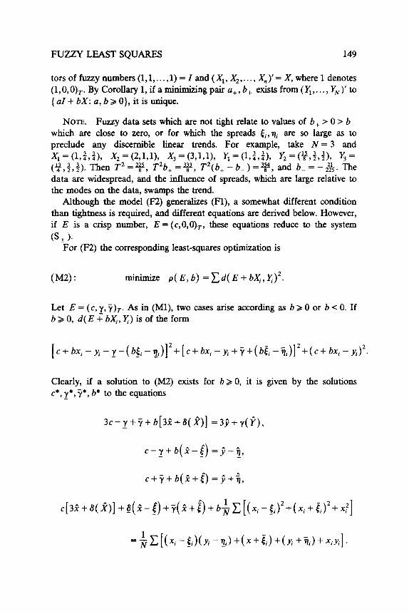
torsoffuzzynumbers(l,l,...,l)=Zand(X,,X,,...,X,)‘=X,whereldenotes

(l,O,O),. By Corollary 1, if a mmimizmgpaira+,b+ existsfrom(Y,,...,Y,)‘to

{ al + bX: u, b > 0}, it is unique.

NOTE. Fuzzy data sets which are not tight relate to values of b, > 0 > b_ which are close to zero, or for which the spreads &, vi are so large as to

preclude any discernible linear trends. For example, take N = 3 and x, = (1 ,$,!), x, = (2,&l), X3 = (3,1,1), r, = (I,!,$), Y7 = <!?,+,t>, r, = (y,t,$). Then T*= y, T*b+=y, T*(b+-b_)=y, and b_=-3. The data are widespread, and the influence of spreads, which are large relative to the modes on the data, swamps the trend.

Although the model (F2) generalizes (Fl), a somewhat different condition than tightness is required, and different equations are derived below. However, if E is a crisp number, E = ( c,O,O)~, these equations reduce to the system

(S, )* For (F2) the corresponding least-squares optimization is

(M2) : minimize p(E,b) =xd(E+bXi,q)*.

Let E = (c, y, Y)T. As in (Ml), two cases arise according as b > 0 or b -C 0. If b>O, d(EjbX,,Y)isoftheform

Clearly, if a solution to (M2) exists for b 2 0, it is given by the solutions c*, y*, y*, b* to the equations -

3c-_v+~+b[32++(Ji!)] =3j+y(f),

c-r+b(R-i) =9-t,

c+v+b(Z++) =j++/,

150 PHIL D~MOND

To simplify the exposition, assume in what follows that E is symmetric, E = (c, y, Y)~; that is, y = r. The equation for b > 0 reduces to

(s*) :

fi+$ i+z y==-z--b=- 2

(8)

(9)

A solution to (M2) for b c 0 and E symmetric is given by replacing (9) and

(IO) by

(Sd:

with (8) unchanged, and will be written as c,, y*, b,. Clearly if y = 0, (S*) and (S,) reduce to the systems (S * ) considered earlier.

DEFINITION 2. For x = (x, $, &, write sp( X) = t f g. The nondegenerate fuzzy data set X,q, i-l ,..., N, is said to be c&erent if the following conditions are satisfied:

(if E[sp( 4) - sp( X)l[sp(Y;) - sp( f)l2 0; (ii) either b, > 0 or b* 6 0.

If b, > 0, the data set is coherent positive, and if b* Q 0 it is coherent negative.

LEBSA 4. For every ~o~dege~erure data set which is coherent,

b* > b*. (11)


Przof. Let T:

(ii - t>f + N&f .k)*.

= 6z{[Xi - 4 + 6(q) - q&p + 2(Xi - a)2 + 2(& - [)

Calculations from (S*) show that

T2b*~6~(3(Xi-~)(~~-~)+(Yi-Y)[6t~)-Yt~)1 1

+(xj-a)[S(~)-6(P)] +(Ei-i)(Tj-t)

and using (S,),

From the coherency condition (i), it is thus sufficient to show T: > 0. Consider the real numbered data set q, z,, i = 1,2,. . . ,3N, which is defined as follows: for i=l,..., N, wi=yj-TJ and zi=xi-&; for i=N+l,..., 2N, y=y, and z.=xi; andfori=2N+l,..., 3N, wi = y, + ii and zi = xi + ii. Clearly (8)-(10) correspond to the classical normal equations for fitting the model w = c + yu + bz,whereuisanindicatorvariable: u,=-lifl<i<N,z+=OifN+lgi< 2N,andui-+lif2N+ldi<3N.ThusT:>O.

NOTE. Reworking the example of widespread data given above, Trr = 5, T,‘b* = 42, T,*b* = 42, T12( b* - b,) = 3, and so b, > 0. The data set is coherent. Observe how the replacement of the crisp constant a by the fuzzy constant E “‘explains” the relatively large spreads and reveals that the modified model now fits the data with a discernible linear trend. As an example of incoherent data, consider X, = (1 2 1 ,4r4), X2 = (l.l,f,L), X, = (1.2,1,1), K = (L$,S), r, = (+$,j,;), Y,=($,$,$)_ Now T’~0.86 T2b*=2.8, T;(b*--b,)=3, and b, < 0. Here the trend on the mc$els of ‘the’data points is out of kilter with trends on the spreads. The “compatibility” of discernible trends on modes and spreads is roughly what coherency means.

TBEOREM 3. The ~rob~ern (M2) has a unique solution if the nondegenerute data set is coherent. If the dotu set is coherent positive, the least-squares fit is given by the (S) system of equations, and if coherent negative by the (S,).

Proof. As in Theorem 2, if the data set is coherent positive, the system (S,) simply cannot arise as a possible solution, and if coherent negative, then (S*) is excluded in a similar way. Let 9(R) consist of all symmetric triangular fuzzy

152 PHIL DIAMOND

TABLE1

(4.0, 0.6, 0.8) (3.0, 0.3, 0.3) (3.5,0.35,0.35) (2.0, 0.4, 0.4) (3.0, 0,3,0.45) (3.5,0.53, 0.7) (2.5,0.25,0.38) (2.5, 0.5, OS)

(21.0, 4.2, 2.1) (15.0,2.25,2.25) (15.0, 1.5,2.25) ( 9.0,1.35,1.35) (12.0, 1.2, 1.2) (18.0, 3.6, 1.8) ( 6.0, 0.6, 1.2) (12.0, 1.8, 2.4)

numbers, and let Y* be the cone in g(#” consisting of elements of the form A+bX,whereb>O,A=(E,E ,..., E)‘,EEY(R),andX=(X,,X,,...,X,)‘. By Corollary 1, if a ~gvector~*+~*Xe~~from(Y~,...,Y~~ tothe cone y*, it is unique. The A*, b* correspond to the solution of (S*) in the coherent positive case. The conclusion for coherent negative data wilI follow in asimilarfashionbyconsidering~~={A-bX:A=(E,...,E)and b>O}.

EXAMPLE 1. A very simple example is taken from 1171, involving student grades and family income. It is not unreasonable to regard both these variables as fuzzy to some extent, and the data were fuzzified as triangular fuzzy numbers as follows:

(1) xi, yj were taken as m(X), m(Y), i =l,..., N; (2) using random digits k from [16], ii etc. were c~c~ated as 10% of xi if

k = 1,2, or 3; 15% of xi if k = 4, 5, or 6; and 20% of xi if k = 7, 8, or 9. Zero digits were discarded.

The result is shown in Table 1, with entries in the form of triangular fuzzy numbers.

Using the model (Fl), it was found that

Y = 1.052+0.147x,

with a sum of residuals 2.898 as compared with 0.713 for the original crisp data. Since T2 =1.612, the formulas of Lemma 3 give b_ = 0.051~ 0, and the data set of Table 1 is tight positive.

Computing with the model (F2) gives

Y= (1.201,0.180,0.180)+0.136X,

with a sum of residuals 2.413. Here T;” = 3156.697, and the formulas of Lemma


4 give b, = 0.131> 0, so the data set is coherent positive.

NUMERICAL INPUT, FUZZY OUTPUT

Suppose that data pairs xi, y, i = 1,. . . , N, are obselved, where the real numbers xi are nonnegative and each I: E y(R). The affine function from R to r(R) defined by

Y=A+xB, x=R, AET(R), BEP(R),

is to be fitted to the data with respect to the best d-fit. Let I be the N-vector (l,l,... ,l)’ and U=(xi,xz ,..., xN)‘. Solutions are sought in either 9?+ = {AI+BU:AET(R), BEB(R)} or V_={AI+BU:AET(R), -BE zP( R)}. In this model, the cones %‘+ or V could be thought of as representing positive or negative fuzzy trends. Writing A = (a, a, (Y)r, B = (b, j3, B)=, con- - sider the problem

(MR): minimize r(A,B) =~d(A+xiB,~)’

If a solution is sought in V+, then

and a similar expression for 64_. If such solutions exist, the parameters of A, B E F(R) satisfy a linear system of six equations in the same number of tuilcnowns, these equations arising from the derivatives of r( A, B) being set equal to zero. For illustrative purposes, attention will be restricted to the case where A, B, q E Y(R) are symmetric triangular fuzzy numbers. This gives a dramatic simplification, but the principles involved are the same as in the more general case and not obscured by tiresome detail.

DEFINITION 3. A nondegenerate data set xi, y = (y, n, q)r, i =l,. . . , N, where each x E Y(R), is said to be cohesive if

$C(Xi-2)(~j-_) >2C(Xi-a)(rli-i) >O* (12)

154 PHIL DIAMOND

NOTE. If the inequalities (12) are reversed, Lemma 5 below shows that a reflection of the explanatory crisp part x, of the data pairs (x,, Y), in the mean P, zi = 22 - xi, renders the data set of pairs (I,, Y) cohesive. If this is done and

Y=A+zB first fitted to {(z,,Y):i=1,2,...,N}, then Y=(A+29B)-xB fits the original data set. Such data sets will also be called cohesive. When the cohesive property is lacking, it demonstrates that there is an underlying incom-

patibility between the trend of modes ): and that of spreads ni, and that the model using crisp input xi is inappropriate. For example, consider data pairs xi =l, Y, = (l,$,$); x2 = 2, Y2 = (y,$,i); x3 = 3, Y, = (y,&,&). The modes have an increasing trend, but the spreads are decreasing. The formal equations

[(13) and Lemma 6 below] give negative spreads for either A or B, an absurdity. This is not to say that a solution to (MR) does not exist-indeed, a minimizing element must exist by Corollary 1. It is just that this solution is not provided by

the equations (13). In the example above, a! > 0 but B < 0 before reflection z = 232 - x, and OL < 0, B > 0 if the data are first reflected.

LEMMAS. Ifthedafusetxi,Y, i=1,2,...,N, issuchrhat 4c(xi-P)(yi-j) <22c(xi-2)(q,-5j)<0, thenzi,q, i=1,2 ,..., N, wherez,=2&-x,, iscohe- sive.

Proof. Now 4,2 are nonnegative and f = 2, so z, - i = 2 - xi and the inequalities reverse to give a relation of the form (12).

LEMMA 6. Let the parameters of A = (a, a, a)r, B = (b, p, f3)r satisfy the system

a = 9 - b2, a=fi-j3A

(13) b = K/T’, /3 = u/T2,

where K=C(xi-2)(y,-j), K=E(x~-~)(~~-?), T2=E(x,-2)2. Suppose the data set is cohesive and nondegenerate. Then a, f3 > 0 and the fuzzy numbers A, B are well defined.

Proof. From (12), (13), (Y, B > 0 iff the data set is cohesive.

THEOREM 4. Let the data set xi, y be cohesive and nondegenerate. If K > K >

0, the problem (MR) has a unique solution in V+ and no solution in V_ , given by (13). Zf K < - K < 0, the problem (MR) has a unique solution in ‘%_ and no solution in W+, given by (13).

Proof. The existence and uniqueness of solutions follows from Corollary 1. The equations (13) arise as necessary conditions to minimize r(A, B) with respect to a, a, b, 8. By Lemmas 5,6, B > 0 if the data are cohesive, and B~g(R)ifb-/3>O.Similarly -BEB(R)if b+/?<O.

FUZZY LEAST SQUARES

y= (Y>%9) x

155

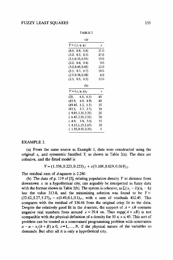
TABLE 2

(a)

(4.0, 0.8, 0.8) 21.0 (3.0, 0.3, 0.3) 15.0 (3.5,0.35,0.35) 15.0 (2.0, 0.4, 0.4) 9.0 (3.0,0.45,0.45) 12.0 (3.5, 0.7, 0.7) 18.0 (2.5,0.38,0.38) 6.0 (2.5, 0.5, 0.5) 12.0

(b)

(21, 6.5, 6.5) 45 (15.9, 4.9, 4.9) 40 (18.45, 1.3, 1.3) 35 (12.5, 2.7, 2.7) 30 ( 9.85,3.35,3.35) 25 ( 6.45,2.55,2.55) 20 ( 4.9, 3.0, 3.0) 15 ( 4.15,1.15,1.15) 10 ( 1.35,0.35,0.35) 5

EXAMPLE 2.

(a) From the same source as Example 1, data were constructed using the

original x, and symmetric fuzzified Y as shown in Table 2(a). The data are

cohesive, and the fitted model is

Y= (1.538,0.223,0.223), + x(0.108,0.019,0.019)r.

The residual sum of d-squares is 2.280. (b) The data of p. 119 of [5], relating population density Y to distance from

downtown x in a hypothetical city, can arguably be interpreted as fuzzy data with the format shown in Table 2(b). The system is cohesive, as X( xi - _?)( vi - 4) has the value 313.0, and the minimizing solution was found to be Y=

(22.62,5.27,5.27),-x(0.49,0.1,0.1),, with a sum of residuals 452.45. This compares with the residual of 336.66 from the original crisp fit to the data. Despite the relatively good fit in the d-metric, the support of A + xB contains negative real numbers from around x = 29.4 on. Thus supp( A + xB) is not compatible with the physical definition of a density for 30 Q x Q 45. This sort of problem can be treated as a constrained programming problem with constraints a-cw-xi(b+j3)>0, i=l,..., N, if the physical nature of the variables so demands. But after all it is only a hypothetical city.

156 PHIL DIAMOND

CONCLUSION

Several models have been proposed for data analysis of fuzzy numbers using a least-squares approach with a suitable metric. The methods are rigorously justified by a projection-type theorem for cones on a Banach space containing the cone of triangular fuzzy numbers. The techniques are simple to apply to actual data sets of such fuzzy numbers. Simple algebraic criteria are given in terms of the data for when it is or is not appropriate to fit a model to a given data set. These are intuitively explained in geometric terms and are the criteria described for tight, coherent, or cohesive data sets, depending on the nature of the model to be fitted.

It is possible to extend this approach to multivariable data (X;:, Y;), where X is a k-vector of triangular fuzzy numbers, and this is described in [15f. Analysis of such models is connately considerably more complicated than the simple linear models treated above. There are 2k cones on which to project, and as yet no simple algebraic criteria have been developed to distinguish them like, for example, those of tight positive or negative in Theorem 2. It seems likely that a selection algorithm, similar to those used in choosing explanatory variates for multilinear statistical regression, will prove useful in this regard.

When the data consist of pairs of fuzzy numbers (4, Y), it is natural to ask whether they can be fitted with models of the form Y = AX+ B, where A, X, and B are fuzzy numbers and AX is fuzzy multiplication. If (X;., Y) are received in the form of triangular or trapezoidal fuzzy numbers, such a fit is not possible, nor would it make good sense. This is because multiplication AX results in members~p functions with due sides (Ch’en 1161) and it is inappropriate to equate a triangular or trapezoidal function with such. It might be possible to fit some data sets ( X, , q), where the membership functions of the X differ from those of the q, by some such model. But this will be a very special case, depending on the type of membership functions not only of X, Y but also of A, B, and it seems likely that much will be lost of the computational simplicity of the models we have discussed.

A simple modification of the metric extends the methodology to the class of trapezoidal numbers 9(R). Denote by Xi the set { t E R : t has a membership grade of 1 for X}. For trapezoidal fuzzy numbers, X1 is a compact interval. If X,Y E?Z(R), define p(X,Y)2=~(~~ppX,s~ppY)2+ 4(X1,Y’)2. This is a metric, and clearly (9”(R), p) is complete. So ~g elements exist in cones in T(R) by an obvious generalization of Theorem 1, and a very similar least-squares method goes through. Other types of fuzzy numbers could be treated with a least-squares approach, but the metrics are more complicated and the simplicity and geometrical intuition are much diminished.

Computational procedures exist also for solving fuzzy relational equations $ = Fe X;, a.U i (sup-min composition); for simple cases see [Z], [3]. As a


general rule these involve large-scale computational schemes and are much

more difficult and complicated problems than the ones addressed here. We have cut our coat to suit our cloth: none of the three models considered need more than a pocket calculator for their fitting.

I would like to thank the referee for suggestions which improved the style and presentation of the paper.

REFERENCES

1. R. E. Bellman and L. A. Zadeh, Decision-making on a fuzzy environment, Management Sci. 17:B141-B164 (1971).

2. D. Dubois and H. Prade, Fuzzy Sets and Systems: Theory and Applications, Academic.

New York, 1980.

3. D. Dubois and H. Prade, Additions of interactive fuzzy numbers, IEEE Trans. Automat.

Central AC-26:926-936 (1981).

4. I. M. Hammerbacher and R. R. Yager, Predicting television revenues using fuzzy subsets,

TIMS Stud. Management Sci. 20~469-477 (1984).

5. L. J. King, Statistical Analysis in Geography, Prentice-Hall, Englewood Cliffs, N.J., 1969.

6. R. E. Moore, Methodc and Applications of Interval Analysis, SIAM, Philadelphia, 1979.

7. C. V. Negoita and D. A. Ralescu, Applications of Fuzzy Sets to Systems Analysis, Wiley,

New York, 1975.

8. H. Prade, Operations research with fuzzy data, in Fuzzy Sets: Theory and Applications to

Policy Analysis and Information Systems (P. P. Wang and S. K. Chang, Eds.), Plenum, New

York, 1980, pp. 115-169.

9. M. L. Puri and D. A. Ralescu, Fuzzy random variables, J. Math. Anal. Appl. 114:409-422

(1986).

10. H. Tanaka et al., Linear regression analysis with fuzzy model, IEEE Trans. Systems Man

Cybernet. SMC-14:325-328 (1984).

11. R. R. Yager, Fuzzy prediction based upon regression models, Inform. Sci. 26:45-63

(1982).

12. L. A. Zadeh, The concept of a linguistic variable and its application to approximate

reasoning, Inform. Sci. 8:199-244, 301-357, 9:43-80 (1975).

13. L. A. Zadeh, Fuzxy sets as a basis for a possibility theory, Fuzzy Sets and Systems 1:3-28 (1978).

14. H. J. Zimmerman, Fuzzy programmin g and linear programming with several objective

functions, Fuzzy Sets and Systems 1:45-55 (1978).

15. P. Diamond, Least squares fitting of several fuzzy variables, in Proceedings of the 2nd

IFSA Congress, Tokyo, July 1987.

16. S. H. Ch’en, Operations on fuzzy numbers with function principle, Tamkang J. Manage-

ment Sci. 6:13-25 (1985) (MR 87a:03088).

Received 26 September 1986; revised 26 May 1987.

Fuzzy Least Squares

Documents

Transcript of Fuzzy Least Squares