Robust Model Predictive Control -...

Robust Model Predictive ControlMotivation: An industrial C3/C4 splitter:

MPC assuming ideal model:

MPC considering model uncertainty

Robust Model Predictive Control

Nominal model of the plant:

0( ) ( )G z G z= + ∆

[ ]0( ) ( ) 1G z G z= + ∆

10 0 0( ) ( ) ( )G z D z N z−=

Norm-bounded uncertainty:

[ ] [ ]10 0( ) ( ) ( )D NG z D z N z−= + ∆ + ∆

Uncertainty is measured through the H infinity norm ∞∆

Closed Loop with Model Uncertainty

K(z) stabilizes the nominal plant G0(z)

Additive uncertainty: 0( ) ( )G z G z= + ∆

( ) 10( ) ( ) ( ) ( )M z K z I G z K z −= +

Small gain theorem:( )( ) 1j TM e ∞∆ <ωσ

( ) 10( ) ( ) ( ) 1j T j T j TK e I K e G e

−

∞ + ∆ <

ω ω ωσ

Closed Loop Stability – Multiplicative Uncertainty

Multiplicative uncertainty: [ ]0( ) ( ) 1G z G z= + ∆

( ) 10 0( ) ( ) ( ) ( )M z K z G z I KG Z −= +

Small gain theorem:( )( ) 1j TM e ∞∆ <ωσ

( ) 10 0( ) ( ) ( ) ( ) 1j T j T j T j TK e G e I K e G e

−

∞ + ∆ <

ω ω ω ωσ

Robust Stability of DMC

Question:

How much model uncertainty a well tuned DMC can tolerate?

[ ] [ ] [ ] / 1/ 1 / 1( 1) F kk k k k k ky A y B u k K y C y− − −= + ∆ − + −

( ) ( 1) ( )TT T T

hy y k y k y k n = + + !

Robust Stability of the Unconstrained DMC

[ ] [ ]/ 1 1/ 1 ( 1)k k k ky A y B u k− − −= + ∆ −

0 0 00 0 0

,0 0 00 0 0

ny

ny

ny

ny

II

AII

=

!!

" " " # "!!

1

2

1

,

h

h

n

n

SS

BS

S +

=

" ,

ny

ny

F

ny

ny

II

KII

=

"

1,1, 1,2, 1, ,

2,1, 2,2, 2, ,

,1, ,2, , ,

i i nu i

i i nu ii

ny i ny i ny nu i

S S SS S S

S

S S S

=

!!

" " # "!

Predicting Model

0 0nyC C I = = ![ ] /( ) k ky k C y=

Robust Stability of the Unconstrained DMCTrue Plant Model

[ ] [ ]/ 1/ 1 ( )k k k ky A y B u k− −= + ∆

DMC control law

[ ] ( ) ( ) [ ] [ ] 1

/ /

T Tm T m T m T sp sps n n n MPCk k k k ku N S Q QS R R S Q QN y y K y y

−

∆ = + − = −

[ ] ( ) ( 1) ( 1)TT T T

ku u k u k u k m ∆ = ∆ ∆ + ∆ + − !

( )

( )

. ( . ) .( 1)

( ) .( 1)

0

0

ny n ny n ny nh

s nu nu nu m

N I

N I

× −

× −

=

=

1

2 1

1 1

1 1

0 00

mn

m m

n n n m

SS S

SS S S

S S S

−

− − +

= " " "

!!

" " # "!

!


Combining predicting model and plant

Additive uncertainty

/ 1/ 1

0( 1)

( ) ( )F F Fk k k k

Ay y Bu k

K CA I K C Ay y B K C B B− −

= + ∆ − − + −

[ ]/ /

( ) 0sp sp

MPC sp spk k k k

y y y yu k K K

y y y y

− −∆ = =

− −

SB B= + ∆1 2 1nh

TT T TS S S S +

∆ = ∆ ∆ ∆ !


Closed loop with DMC

[ ] [ ] 1 21/ 1 / ( ) ( )k k k ky y u k u k+ + = + ∆ + ∆$ $φ β β

0( )F F

AK CA I K C A = −

φ 1BB

=

β '2 2S S

F

IK C

= ∆ = ∆

β β

/

( )sp

spk k

y yu k K

y y

−∆ =

−

11 1 '1 2( ) ( ) ( )M z K I zI K zI

−− − = − + − − φ β φ β


Example 1

11 1 '1 2( ) ( ) ( )M z K I zI K zI

−− − = − + − − φ β φ β

11 12

21 22

1.77 5.8860 1 50 1( )

4.41 7.244 1 19 1

s sG s

s s

+ ∆ + ∆ + += + ∆ + ∆ + +

DMC parameters: T=5, n=12, m=5, Q=diag(1,1), R=diag(0.3,0.3)

Question: What is the max size of ∆11, ∆12, ∆21 and ∆22 such that DMC will remain stable?

Response: DMC will be stable for ∆S not larger than

( ) 1min( )S TiM e

∆ =

ωωσ

σ

Example 1 DMC with: T=5, n=12, m=5, Q=diag(1,1), R=diag(0.3,0.3)

The approximate bounds are:

1min 1.195( )TiM e

=

ωω σ

, , , , , ,0.13 0.13 1,2; 1,2; 1, ,12i j l i j l i j lS S S i j l− ≤ ≤ + = = = …

Or: ,0.13 0.13 1,2; 1,2i j i j− ≤ ∆ ≤ + = =

Example 1 Stability bounds are very conservative


1.77 0.13 5.88 0.1360 1 50 1( )

4.41 0.13 7.2 0.1344 1 19 1

s sG s

s s

+ − + += − + + +



1.77 0.3 5.88 0.360 1 50 1( )

4.41 0.3 7.2 0.344 1 19 1

s sG s

s s

+ − + += − + + +


1.77 0.9 5.8860 1 50 1( )

4.41 7.244 1 19 1

s sG s

s s

− + += + +

Robust Stability - Multiplicative gain uncertainty

/ 1/ 1

0( 1)

( ) ( )F F Fk k k k

Ay y Bu k

K CA I K C Ay y B K C B B− −

= + ∆ − − + −

SB B= + ∆( ),1ij ij i jB B= + ∆

1,1 1,2 1,

2,1 2,2 2,

,1 ,2 ,

0 0 0 0 0 00 0 0 0 0 0

0 0 0 0 0 0

nu

nuS

ny ny ny nu

S S SS S S

S S S

∆ = ×

! ! ! !! ! ! !

" " # " " " # " ! " " # "! ! ! !

1,1

,1

1,

,

1 0 00

0 1 00 1 0

0 1 00 0 0 1

0 0 1

ny

nu

ny nu

nu

∆ ∆ ∆ ∆

!" " !

# ! "!

# " " ! "!

# !" " ! "

!&''('')S K uS N∆ = ∆$

[ ] [ ] 1 21/ 1 / ( ) ( )k k k ky y u k u k+ + = + ∆ + ∆$ $φ β β

0( )F F

AK CA I K C A = −

φ 1BB

=

β 2 2K u K uF

BN N

K CB

= ∆ = ∆

$$

$β β

Robust Stability - Multiplicative gain uncertainty

=

11 11 2( ) ( ) ( )uM z N K I zI K zI

−− − = − + − − $φ β φ β

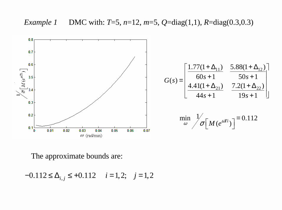
Example 1 DMC with: T=5, n=12, m=5, Q=diag(1,1), R=diag(0.3,0.3)

The approximate bounds are:

1min 0.112( )TiM e

=

ωω σ

,0.112 0.112 1,2; 1,2i j i j− ≤ ∆ ≤ + = =

11 12

21 22

1.77(1 ) 5.88(1 )60 1 50 1( )

4.41(1 ) 7.2(1 )44 1 19 1

s sG s

s s

+ ∆ + ∆ + += + ∆ + ∆ + +

Example 1 Gain uncertainty - Stability bounds are not so conservative

1.77(1 0.11) 5.88(1 0.11)60 1 50 1( )

4.41(1 0.11) 7.2(1 0.11)44 1 19 1

s sG s

s s

− + + += + − + +

,0.112 0.112 1,2; 1,2i j i j− ≤ ∆ ≤ + = =

Example 1 Gain uncertainty - Stability bounds are not so conservativebut misses some particular systems

1.77(1 0.5) 5.8860 1 50 1( )

4.41 7.244 1 19 1

s sG s

s s

+ + += + +

,0.112 0.112 1,2; 1,2i j i j− ≤ ∆ ≤ + = =

Robust Stability with H∞ Approach

-The ranges of general unstructured model uncertainties where DMC is guaranteed to be stable are quite conservative. Less conservative bounds can be obtained by taking into account the structure of the uncertainty. However, the results are still not useful for practicalapplications.

-The procedure does not account for constraints on the inputs and input moves. When a constraint becomes active, the closed loop system may become unstable, even if uncertainty is smaller than the maximum uncertainty tolerated by the unconstrained DMC controller.

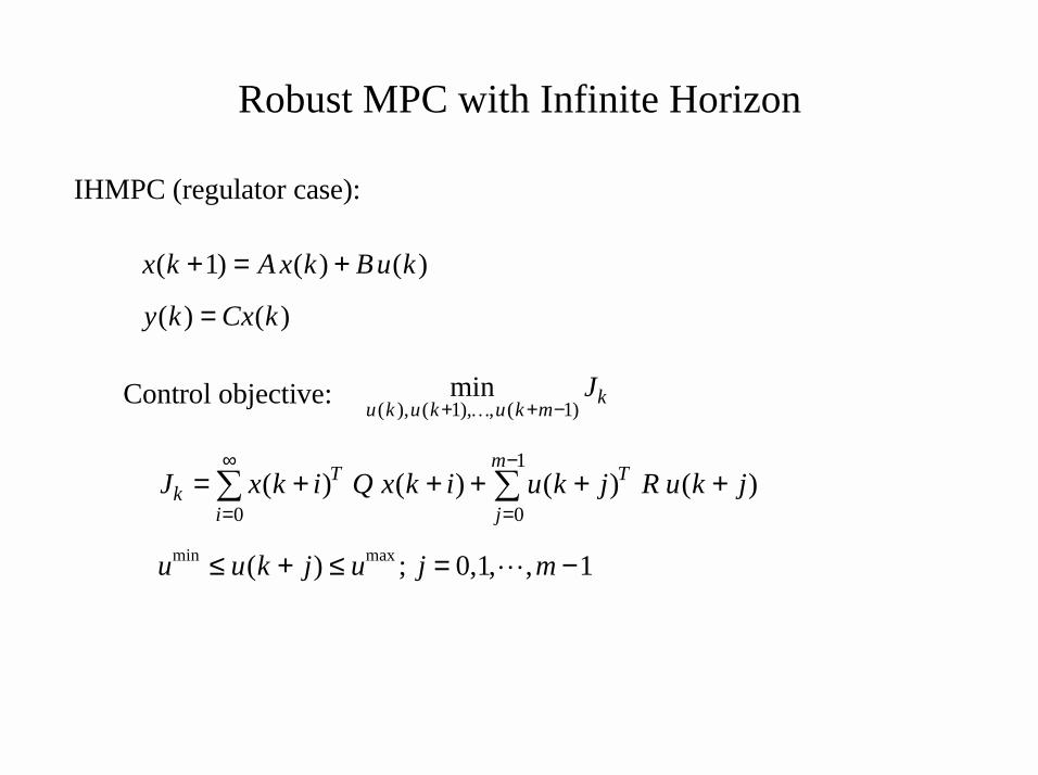
Robust MPC with Infinite Horizon

IHMPC (regulator case):

( 1) ( ) ( )x k A x k Bu k+ = +

( ) ( )y k Cx k=

Control objective: ( ), ( 1), , ( 1)min ku k u k u k m

J+ + −…

1

0 0( ) ( ) ( ) ( )

mT Tk

i jJ x k i Q x k i u k j R u k j

∞ −

= == + + + + +∑ ∑

min max( ) ; 0,1, , 1u u k j u j m≤ + ≤ = −!

Robust MPC with Infinite HorizonIHMPC (regulator case) for stable systems:

( ), ( 1), , ( 1)min ku k u k u k m

J+ + −…

min max( ) ; 0,1, , 1u u k j u j m≤ + ≤ = −!

1

0 0( ) ( ) ( ) ( ) ( ) ( )

m mT T Tk

j jJ x k j Q x k j x k m Px k m u k j Ru k j

−

= == + + + + + + + +∑ ∑

TA PA P Q− = −

Advantage: The closed-loop is stable for any set of tuning parameters

Drawback: Cannot be applied to the set point tracking caseModel is written in terms of and ssu u− ssy y−

Robust MPC with Infinite HorizonRobust IHMPC (regulator case):

( 1) ( ) ( )x k A x k Bu k+ = +( ) ( )y k Cx k=

( , )A B=θ

( , )T T T TA B= ∈Ωθ θ

Multi plant system: 1 2, , , LΩ * …θ θ θ

True plant:

Nominal plant: ( , )N N N NA Bθ θ= ∈Ω

1

,0 0

( ) ( ) ( ) ( ) ( ) ( )i i i i i i

m mT T Tk

j jJ x k j Q x k j x k m P x k m u k j Ru k j

−

θ θ θ θ θ θ= =

= + + + + + + + +∑ ∑

i i i iTA P A P Qθ θ θ θ− = −

Robust MPC with Infinite HorizonRobust IHMPC (regulator case) is obtained from the solution to:

,( ), ( 1),..., ( 1)min

Nku k u k u k mJ

+ + − θ

Subject to:

, ,ˆ

i ik kJ J≤θ θ i ∈Ωθmin max( ) ; 0,1, , 1u u k j u j m≤ + ≤ = −!

,ˆ ( 1,..., )

ikJ i L=θ is obtained with the following control sequence:* *

1ˆ ( ) ( 2) 0k ku u k u k m

− = + − !

* * *( ) ( 1) ( 1)k ku u k u k u k m ⇒ = + + − !

Robust IHMPC (regulator) cannot be applied to the set-point tracking:

is not bounded for all plants with different gains. iθ ∈Ω,ˆ

ikJ θ

Extended Infinite Horizon MPC

Process model in the incremental form:

0( 1) ( )( )

0( 1) ( )

s s sny

d d d

Ix k x k Bu k

Fx k x k B+ = + ∆ +

( )( )

( )

s

ny d

x ky k I

x k

= Ψ

( ) ( ) ( 1)u k u k u k∆ = − −

Control objective:

1

0 0( ( ) ) ( ( ) ) ( ) ( )

mTT T

k k k k kj j

V e k j Q e k j u k j R u k j S∞ −

= == + − δ + − δ + ∆ + ∆ + + δ δ∑ ∑

( ) ( ) spe k j y k j y+ = + −

Extended IHMPC

Problem P2:

Subject to:

,min

k kk

uV

∆ δ

( ) ( )0

-1

0

( ) ( ) ( ) ( )

( ) ( )

m T d T dk k k

j

mT T

k kj

V e k j Q e k j x k m Q x k m

u k j R u k j S

=

=

= + − δ + − δ + + +

+ ∆ + ∆ + + δ δ

∑

∑T T TQ F QF F Q F− = Ψ Ψ

( ) 0s sk ke k B u+ ∆ − δ =$ [ ]s s s

m

B B B=$ !&''('')max max

min max

0

( )

( 1) ( ) ; 0,1, , 1j

i

u u k j u

u u k u k i u j m=

−∆ ≤ ∆ + ≤ ∆

≤ − + ∆ + ≤ = −∑ !

[ ]( ) ( 1) ( 1)k ku u k u k u k m∆ = ∆ ∆ + ∆ + −!

Extended Robust IHMPC

Problem P3:

Subject to:

, , 1,...,,

,min N

k k i Lik

uV

θθ

δ =∆

,( ) 0 1,...,i

s si k ke k B u i Lθ+ ∆ − δ = =$

max max

min max

0

( )

( 1) ( ) ; 0,1, , 1j

i

u u k j u

u u k u k i u j m=

−∆ ≤ ∆ + ≤ ∆

≤ − + ∆ + ≤ = −∑ !

, ,ˆ 1,...,

i ik kV V i Lθ θ≤ =

,ˆ

ikV θ is computed with: and ˆku∆ ,ˆ

ik θδ

* *1

ˆ ( ) ( 2) 0−

∆ = ∆ ∆ + − !k ku u k u k m

,ˆˆ( ) 0 1,...,θ+ ∆ − δ = =$

is s

i k ke k B u i L

Robust Extended IHMPC

Example 2 : The high purity distillation column

1 1 2 1

2 1 2 2

( ) 0.7868(1 ) 0.6147(1 ) ( )1( ) 0.8098(1 ) 0.982(1 ) ( )22.98 1

+ γ − +γ = + γ − + γ+

y s u sy s u ss

1 20.4 , 0.4Ω ⇒ − ≤ γ γ ≤

[ ](0,0) ( 0.4, 0.4) ( 0.4,0.4) (0.4, 0.4) (0.4,0.4)Ω ≅ − − − −

Tuning parameters of RE-IHMPC: T = 2, m = 3, Q = diag(1, 1), R = diag(10-2,10-2),

S = diag(102,102), ∆umax = 0.25, umax = 1.5, umin = -1.5

Example 2 ( ) ( )1 2, 0,0γ γ =Nominal model:

Case 1: true plant is ( ) ( )1 2, 0,0γ γ =Case 2: true plant is ( ) ( )1 2, 0.4, 0.4γ γ = − −Case 3: true plant is ( ) ( )1 2, 0.4,0.4γ γ = −

( )( - - - -)

( ⋅ ⋅ )

Example 2 RE-IHMPC with input saturation: Case 2: with umax = 0.5

Robust Stability with IHMPC

Advantages:-Quite large ranges of model uncertainties can be considered in the

MPC control law computation. -The structure of MPC is preserved (constraints are included) andcan be implemented in practice.

-Performance is expected to deteriorate if uncertainty is too large but better than the controller with nominal model.

Disadvantages:-Computer effort tends to be larger than in the nominal MPC. Should be applied only in subsystems where uncertainty is critical.

-Still lacking a practical solution to integrating and unstable systems.

Robust Model Predictive Control -...

Documents

Transcript of Robust Model Predictive Control -...