Process Control Design WorkshopSolutions...

Copyright © 2005 by T. Marlin 1

Process Control Design

Solutions for PASI Workshops

This document contains solutions for most of the workshops in the Lesson on “Process Control Design” presented at the PASI Course at Iguazu Falls on August 16-25, 2005. The workshops are designated by the main topic and the workshop number within the topic. The following table of contents enables you to quickly find the solution you seek. Workshop No. Topic

Page No.

Defining the Control Problem 1 Control Design Form for a Distillation Tower No solution 2 Control Design Form for a Fired Heater No solution 3 Information for design from a Flowsheet No solution 4 Strategies for Reduced Variance 3 5 Assumption in Benefits Calculation 4 6 Optimum Variance for Several Performance Correlations 5

Single-Loop Feedback Control 1 Large range in a Manipulated variable 7 2 Using the Optimum manipulated variable 8 3 Minimizing flow to waste 9 4 Heat Exchanger Control - Three designs 10 5 Distillation Tower Pressure Control - Using Cooling Water 11 6 Distillation Tower Pressure Control - Using Refrigeration 12 7 PH Control for Strong Acid/Base 13

Interaction 1 Operating Window for a Blending Process 14

Controllability 1 Controllability of a Mixing Process 15 2 Controllability of Boiler Temperature and Pressure 16 3 Controllability of Flash Temperature and Pressure 17 4 Controllability of a CSTR 18

Integrity 1 Integrity of Controls for a Head Box 20 2 Integrity of Controls for a Distillation Tower - Energy Balance 21 3 Integrity of Controls for a Distillation Tower - Material Balance 23 4 Integrity of Controls for a 4x4 Process 24 5 Effect of Regulatory Controls and Operating Conditions on Integrity 25


Directionality and Performance 1a Directionality for single Set Point Change 26 1b Directionality for disturbance through manipulated variable process 28 1c Directionality for one-way interaction 29 1d Considering Input Directionality in Decoupling 30 2 Analysis of a distillation tower with tray temperatures 31

Short-Cut Design Procedures 1A Selecting Controlled Variables for Seven Categories of Objectives 32 1B Selecting Manipulated Variables 46 1C Check if Achieving Control Objectives is Possible 47 1D Eliminating Unacceptable Design Candidates 48 2 Maleic Anhydride Feed Vaporizer 50 3 Fuel Gas Distribution 52 4 Vapor Compression Refrigeration 54 5 Flash Separation Process 56 6 CSTR with Recycle 59 7 Two Units with Intermediate Storage 67 8 Liquid-Liquid Decanter 69 9 Hydrocracker - Packed Bed Reactors with Exothermic Reaction 70

10 Optimize Preheat 71-73


Defining the Control Problem

Two process examples show the benefit of reduced variability, the fired heater reactor and the boiler. Discuss the differencebetween the two examples. Can you think of another example that shows the principle of each?

0

0.1

0.2

0.3

0.4

frequency of occurrence

-3 -2 -1 0 1 2 3 deviation from mean

Squeeze down the variability

DEFINING THE PROBLEM: Workshop 4


The principle involves using the entire distribution to evaluateperformance. This is the same for both examples.

They differ in the actions taken to improve performance.

• In Case A the action involved reducing the variability (through improved control) and taking advantage of the reduced variance by changing the set point closer to an inequality constraint. Someprocess examples include

i. Maximizing the production of an existing process by operatingnear equipment limitation (distillation tray hydraulics, pumping, hest transfer, etc.)

ii. Operating near limits to reduce manufacturing costs, for example, minimum distillation pressure and minimum disillation reflux ratio (that achieves desired separation)


The principle involves using the entire distribution to evaluateperformance. This is the same for both examples.

They differ in the actions taken to improve performance.

• In Case B the action involved reducing the variability (through improved control) while maintaining the variable average at its desired value. Some process examples include

i. Reducing variability in key product qualities (paper thickness, polymer molecular weight, and the color of ink or paint.

Note that the customer requires the same quality all of the time. If the paper jams in your printer because it is too thick, you will not appreciate the supplier telling you that you obtained “extra” paper.




Discuss an important assumption that is made on the procedure proposed for calculating the average process performance. (Hint: consider dynamics)

How would you evaluate the assumption?

Note that the histogram summarizes the dynamic plant data. The data contains no information on the frequency content.

The “Process Performance” correlation is nearly always based on steady-state behavior of the process.

The key assumption is that each instant of the dynamic operation represents a “quasi-steady state”, in which the process performance correlation is valid.

Dynamic data

Steady-state model





The following performance vs. process variable correlations are provided. All applications require the same average valuefor the process variable (see arrow). What is the best distribute for each case? (Sketch histogram as your answer.)

Process variable

Dis

trib

utio

n Pr

oces

s per

form

ance

Process variable

Dis

trib

utio

n Pr

oces

s per

form

ance

BA

Process variable

Dis

trib

utio

n Pr

oces

s per

form

ance

C


Process variable

Dis

trib

utio

n Pr

oces

s per

form

ance

Any distribution with the required mean value for the variable will have the same process performance, because the performance is linear with the variable!

A

Process variable

Dis

trib

utio

n Pr

oces

s per

form

ance

Average performance

Average performance



A narrow distribution about the average value will yield the highest average profit!

This is the typical process situation.B

Average performance

Average performance

Process variable

Dis

trib

utio

n Pr

oces

s per

form

ance

Process variable

Dis

trib

utio

n Pr

oces

s per

form

ance


A broad distribution about the average value will yield the highest average profit!

This is not the typical process situation.C

Average performance

Average performance

Process variable

Dis

trib

utio

n Pr

oces

s per

form

ance

Process variable

Dis

trib

utio

n Pr

oces

s per

form

ance


Single-Loop Feedback Control

Feed

MethaneEthane (LK)PropaneButanePentane

Vaporproduct, C2-

Liquidproduct, C3+Steam

F3

T3

T5

TC6 PC1

LC1

A1

L. Key

What if the % ethaneis sometimes 2%

and other times 50%?

Single-loop Control, Workshop #1

Feed


Vaporproduct, C2-

Liquidproduct, C3+Steam

F3

T3

T5

TC6 PC1

LC1

A1

L. Key

What if the % ethaneis sometimes 2%

and other times 50%?





The consumers vary and we must satisfy them by purchasing fuel gas. Therefore, we want to control the pressure in the gas distribution network. Design a control system. By the way, fuel A is less expensive.


The two valves are calibrated so that A opens from 0-50% of signal and valve B opens from 50-100% of signal.




Design a controller that will control the level in the bottom ofthe distillation tower and send as much flow as possible to Stream A




Freedom to adjust flows

Stream A Stream B

1. Constant Adjustable

2. Adjustable Constant

3. Constant Constant

Stream A(cold)

Stream B(hot)

TC1

Stream A(cold)

Stream B(hot)

TC

3

Stream A(cold)

Stream B(hot)

TC

2


You can add valve(s) and piping.

Freedom to adjust flows

Stream A Stream B

1. Constant Adjustable

2. Adjustable Constant

3. Constant Constant

Stream A(cold)

Stream B(hot)

TC1

Stream A(cold)

Stream B(hot)

TC

3

Stream A(cold)

Stream B(hot)

TC

2

It is not typical to adjust a stream flow to control its temperature; if the temperature is important, likely the flow rate is also. But, the design will function




CW

NC

Class exercise: Distillation overhead system. Design a pressure controller. (Think about affecting U, A and ∆T)


PC

No vapor product


CW

PC

LC

NC

NOTES• Changes LMTD and hi

• Response is slow & non-linear

• The cooling water can become too hot, leading to excessive fouling (Tcout < 50C)

Not recommended!

Class exercise: Distillation overhead system. Design a pressure controller.


Affecting U & ∆T

CWPC

LC

NC

Fully open NOTES• The liquid in the condenser

affects the area on the hot side

• Generally fast response

• Widely used in practice

Recommended



Affecting A



Class exercise: Distillation overhead system. Design a pressure controller. (Think about affecting U, A and ∆T)


Refrigerant

NCLC

PC




Affecting A

Refrigerant

NCLC

PC NOTES• Generally acceptable

speed of response

• Valve in refrigerant liquid affects the area for heat transfer on cooling side

OK, best efficiency

Refrigerant

NC

LC

LC

PC NOTES• Very fast response

• Valve in refrigerant vapor increases pressure drop through refrigeration cycle and lowers efficiency

OK, slightly lower efficiency



Affecting A



L

A1C

Strong base

F1

Strongacid

The following control system has a very large gain near pH = 7. For a strong acid/base, performance is likely to be poor. How can we improve the situation?

pH


L

A1C

Strong base

F1

Strongacid

L

A2C

VC

large

small

Controller adjusts the large valve only when the small valve is near saturation. This feedback controller has a deadband.

Variable structure control (valve-position controller) can provide good control over a large range because the high frequency disturbances are corrected using the high resolution, small valve.

If this had only the small valve - poor range

If this had only the large valve - poor resolution

pH

pH

Second tank reduces high frequency variations



Interaction

Multivariable Interaction, Workshop #1

0

10

20

30

40

50

60

70

80

90

100

0.00 0.1 0.2 0.3 0.4 0.5 0.6 0.7 0.8 0.9 1.00

Composition (fraction A), xAM

Tota

l flo

w, F

M

The ranges of the two mixing flows are given in the figure.

Sketch the feasible steady-state operating window in the Figure.

Note:

You may assume no disturbances for this exercise.

FA, xA=1FS, xAS = 0 FM, xAM

0-30 m3/h

0-60 m3/h

Multivariable Interaction, Workshop #1

We see that because of interaction, the steady-state feasible region (operating window) is not a rectangle.

FA, xA=1FS, xAS = 0 FM, xAM

0-30 m3/h

0-60 m3/h

0

10

20

30

40

50

60

70

80

90

100

0.00 0.1 0.0 0.3 0.4 0.5 0.6 0.7 0.8 0.0 1.00

Composition (fraction A)

Tota

l flo

w, F

3

infeasible

feasible


Controllability

We need to control the mixing tank effluent temperature and concentration.

You have been asked to evaluate the steady-state controllability of the process in the figure.

Discuss good and poor aspects and decide whether you would recommend the design.

F1T1CA1

F2T2CA2

T

A

CONTROLLABILITY : Workshop 1

Controlled variables are the temperature and concentration in the tank effluent.


Answer based on process insight for the mixing process.

We can plot the operating window, which is shown in the figure. We see that the window is a line, operations off of the line are not possible. Clearly, the process is not controllable; i.e., we cannot achieve arbitrary values of the temperature and concentration.

Also, we note that an arbitrary temperature would be achieved by adjusting the ratio of flows F1/(F1+F2). However, the arbitrary concentration would be achieved by adjusting the same ratio. Therefore, the process is not controllable.

T1 T2

CA1

CA2

Operating window


A more formal approach would be to linearize the process model about the operating point and evaluate the gain matrix.

−−−−

=

'

2

'1

221121

221121'

'

)()()()(

FF

TTTTCCCC

TC

ss

sAAsAAA

αααα

221

12

221

21

)(

)(

ss

s

ss

s

FFF

FFF

+=

+=

α

αwith

We observe that the gain matrix has dependent rows and columns. Therefore, the matrix is singular, and the system is not controllable.


Controllability

The sketch describes a simplified boiler for the production of steam. The boiler has two fuels that can be manipulated independently. We want to control the steam temperature and pressure. Analyze thecontrollability of this system and determine the loop pairing.



The pressure and temperature of saturated steam are related through equilibrium; see the steam tables. It is not possible to control T and P to independent values.

The system is not controllable!


Controllability

The sketch describes a simplified flash drum. A design is proposed to control the temperature and pressure of the vapor section. Analyze the controllability of this system and determine if the loop pairing is correct.

vapor

liquid

Hot streams


Feed


The question is whether the temperature and pressure of this two-phase system are independent. For a multicomponent system, the variables are independent, as shown in the standard figure below, with P1<P2<P3.


Fraction of light key

Tem

pera

ture

P1

P2

P3Also, we see that valve v1 affects the temperature and v5 affects the pressure.

Therefore, the system is controllable, in at least the steady-state sense.


Controllability

A non-isothermal CSTR

• Does interaction exist?

• Are the CVs (concentrations) independently controllable?

A → B + 2C-rA = k0 e -E/RT CA

A

ACB

CC

+ +

+ +

G11(s)

G21(s)

G12(s)

G22(s)

Gd2(s)

Gd1(s)v1

v2


non-isothermal CSTR

• Are the CVs independently controllable?



A

ACB

CC

v1

v2

Using the symbol Ni for the number of moles of component “i” that reacts, we have the following.

ACAB NNNN 2−=−=

Because of the stoichiometry,

NC = 2 NB

and the system is not controllable!

Solution continued on

next slide

CONTROLLABILITY


Controllability

non-isothermal CSTR

• Are the CVs independently controllable?



A

ACB

CC

v1

v2

Solution continued on

next slide

=

=

2

1

2121

1111

2200

MVMV

KKKK

CC

C

B

Det (K) = 0; not controllable!

CONTROLLABILITY

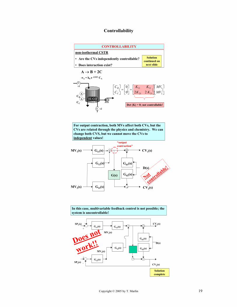
For output contraction, both MVs affect both CVs, but the CVs are related through the physics and chemistry. We can change both CVS, but we cannot move the CVs to independent values!

+

+

G11(s)

G22(s)

Gd2(s)

Gd1(s)D(s)

CV1(s)

CV2(s)MV2(s)

MV1(s)

G12(s)

+

G(s)

“output contraction”

Not

controllable!

+-

++

+ +-

+

Gc1(s)

Gc2(s)

G11(s)

G12(s) Gd2(s)

Gd1(s)

D(s)

CV1(s)

CV2(s)

MV2(s)

MV1(s)

SP1(s)

SP2(s)

Does not

work!!

In this case, multivariable feedback control is not possible; the system is uncontrollable!

Solutioncomplete


Integrity

The process in the figure is a simplified head box for a paper making process. The control objectives are to control the pressure at the bottom of the head box (P1) tightly and to control the slurry level (L) within a range. The manipulated variables are the slurry flow rate in (Flin) and the air vent valve opening.

Integrity Workshop 1

1. Determine the integrity of the two possible pairings based process insight.

2. Recommend which pairing should be used.

3. Discuss the integrity of the resulting system.

Pulp and water slurry

Paper mat on wire mesh

Air

The key factor in analyzing this system is the open-loop dynamics which are discussed qualitatively below.

1. For an increase in the slurry flow in (with the vapor valve constant) both the level and the pressure at the bottom of the head box increase. At the new steady state, the flows in and out are equal; since the flow out depends on P1, it must increase.

2. For an increase in the opening of the vapor valve (with constant slurry flow in) the pressure P decreases. At the new steady state, the flows in and out are equal; thus P1 must be unchanged. P1 is constant because the level and pressure P change in compensating directions.

As a result, there is no steady-state causal relationship between the vapor valve and the flow out Flout, although this is the fastest influence on the flow out, not requiring a change of the slurry inventory. However, we want the fast respose for tight control of P1.

Pairing the loops as shown in the following figure involves pairing on a relative gain of zero.

This is probably the best control design, but requires a monitoring program to ensure that the level controller is functioning (in automatic with the manipulated variable not at an upper or lower bound). If the level controller is not functioning, the P1 controller must be placed in manual and an alarm annunciated to inform the operator.


For model, see McAvoy, T., IEC PDD, 22, 42-49 (1982)


Air

Pulp and water slurry


Integrity

AC

AC

The following transfer function matrix and RGA are given for a binary distillation tower. Discuss the integrity for the two loop pairings.

+−

+

+−

+=

−−

−−

)()(

12.101253.0

175.111173.0

1150667.0

1120747.0

)()(

23.3

23

sFsF

se

se

se

se

sXBsXD

V

Rss

ss

1.61.5 1.51.6

−−

XBXD

FVFR


AC

AC

1.61.5 1.51.6

−−

XBXD

FVFR


The pairing in the accompanying figure has good integrity. If one loop is placed in manual, the sign of the controller gain for stabilizing control will be unchanged.

There is no guarantee that one loop with the same tuning will be stable for both statuses (on/off) of an interacting loop.


Integrity

1.61.5 1.51.6

−−

XBXD

FVFR


The pairing in the accompanying figure has poor integrity. However, it can function if the sign of one controller is switched from its proper single-loop sign.

If the interacting loop is placed in manual, the remaining single-loop controller (with the switched sign) will be unstable.

AC

AC

0 100 200 300 4000.975

0.98

0.985

0.99

0.995IAE = 0.3338 ISE = 0.0012881

XD, D

istil

late

Lt K

ey

0 100 200 300 4000.005

0.01

0.015

0.02

0.025

0.03IAE = 0.58326 ISE = 0.0041497

XB, B

otto

ms

Lt K

ey

0 100 200 300 400 50013.3

13.4

13.5

13.6

13.7

13.8

Time

Reb

oile

dV

apor

0 100 200 300 400 5008.5

8.6

8.7

8.8

8.9

9

Time

Ref

lux

Flow

Stable multiloop feedback control

AC

AC

XF


An example of stable multiloop control with pairing on a negative relative gain. (The bottoms (XB) controller has a sign opposite needed to stabilize the single-loop situation.)


Integrity

The following transfer function matrix and RGA are given for a binary distillation tower. Discuss the integrity for the two loop pairings.

AC

AC

XD

XB

FD

FV

XF

+−

+−

++−

=

−−

−−

)()(

13008.0

175.111173.0

15008.0

1120747.0

)()(

23.3

23

sFsF

se

se

se

se

sXBsXD

V

Dss

ss

39.061.0 61.039.0

XBXD

FVFD



39.061.0 61.039.0

XBXD

FVFDAC

AC

XB

FD

FV

XF

AC

AC

XB

FD

FV

XF

Both of the designs in the figures have acceptable integrity. That does not mean that

• Their dynamic performance is acceptable

• If one controller is in manual, the other will be stable in single-loop


Integrity

0100483.10083.383.0083.12

001014321

CVCVCVCV

mvmvmvmv

−−


We will consider a hypothetical 4 input, 4 output process.

• How many possible combinations are possible for the square mutliloop system?

• For the system with the RGA below, how many loop pairings have good integrity?


The number of loop pairings for an nxn process is n!. For the 4x4 system, the number of loop pairings is 4! = 4*3*2*1 = 24.

Only one loop pairing for the following RGA.

0100483.10083.383.0083.12

001014321

CVCVCVCV

mvmvmvmv

−−


Integrity

XD, XB FeedComp.

RGA RGA

.998,.02 .25 46.4 .07

.998,.02 .50 45.4 .113

.998,.02 .75 66.5 .233

.98, .02 .25 36.5 .344

.98, .02 .50 30.8 .5

.98, .02 .75 37.8 .65

.98, .002 .25 66.1 .787

.98, .002 .50 46 .887

.98, .002 .75 48.8 .939

Small distillation column

Rel. vol = 1.2, R = 1.2 Rmin

From McAvoy, 1983


AC

AC

XD

XB

FR

FV

XF

AC

AC

XD

XB

FD

FV

XF

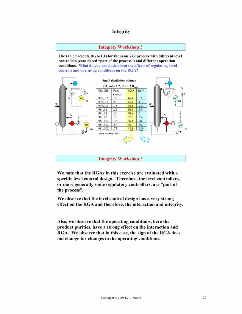
The table presents RGA(1,1) for the same 2x2 process with different level controllers (considered “part of the process”) and different operation conditions. What do you conclude about the effects of regulatory level controls and operating conditions on the RGA?


We note that the RGAs in this exercise are evaluated with a specific level control design. Therefore, the level controllers, or more generally some regulatory controllers, are “part of the process”.

We observe that the level control design has a very strong effect on the RGA and therefore, the interaction and integrity.

Also, we observe that the operating conditions, here the product purities, have a strong effect on the interaction and RGA. We observe that in this case, the sign of the RGA does not change for changes in the operating conditions.


Directionality and Performance

Directionality & Performance Workshop 1

Prove the following important results.

A. For a single set point change, RDG = RGA

B. For a disturbance with same effect as an MV, the RDG = 0 to 2.0 (depending on the output variable)

C. For one-way interaction, RDG = 1

D. Decouple only for unfavorable directionality, i.e., large RDG

Evaluate the RDG and integral errors for this special case,

Set point change: Kd1 = ∆SP1 Kd2 = ∆SP2 = 0

∫

∫

dttE

dttE

)(

)(

2

1

What is the RDG equal to in this case?

∫ ∫∞ ∞

=0 0

)( )( dttEfRDGdttE iSLtuneijiML







SLc

ID

SLc

IDD

SL

c

IDD

KKT

KfKKRGA

KKT

fK

KKKRGAdttE

EfRGA

KKT

fK

KKKRGAdttE

)(**

)(*)()(

**

)(*)()(

222

21detune

11

2122

222

2detune

11

2112222

1detune11

111

1detune

22

1221111

−

−=

−−=

=

−−=

∫

∫

∫

∫ ∫∞ ∞

=0 0


Basic conclusion?





∫ ∫∞ ∞

=0 0


∫∫ = 1detune111 **)( SLEfRGAdttE

)(**)( 2detune11

21222 ∫∫

= SLEf

KKRGAdttE

CONCLUSIONS• The RDG=RGA for this

disturbance

• For large |RGA| systems, changing a single set point will lead to poor performance (relative to single-loop)







∫ ∫=∞ ∞

0 0dttEfRDGdttE SLtuneML )( )(


Disturbance through MV process: Kd1 = K11 Kd2 = K22

∫

∫

dttE

dttE

)(

)(

2

1

∫ ∫=∞ ∞




0

)(*)()(

**)/(

)(*)()(

222

2detune

11

2112222

1detune1detune1111

111

1detune

22

1221111

=

−=

==

−−=

∫

∫∫

∫

c

DD

SLSL

SLc

DD

KKTIf

KKKKRGAdttE

EfEfRGARGA

KKTIf

KKKKRGAdttE



0)(

*)(

2

1detune1

=

=

∫

∫∫

dttE

EfdttE SL


CONCLUSIONS• The RDG ≈ 1 for this

disturbance

• For disturbances through the MV process, the control performance will be likely close to single-loop

∫ ∫=∞ ∞









∫ ∫=∞ ∞



One-Way Interaction: K12 ≠ 0 K21 = 0

∫

∫

dttE

dttE

)(

)(

2

1

∫ ∫=∞ ∞




∫

∫

∫

∫

=

−−=

−=

−−=

2

222

2detune

11

2112222

1221

122

111

1detune

22

1221111

)(*)()(

*)1(

)(*)()(

SL

SLc

DD

SLD

D

SLc

DD

E

KKTIf

KKKKRGAdttE

EKKKK

KKTIf

KKKKRGAdttE

1 1

1 1




∫ ∫=∞ ∞




∫∫

∫∫

=

−=

22

1221

1221

)(

*)1()(

SL

SLD

D

EdttE

EKKKK

dttE

CONCLUSIONS• The RDG ≈ 1 for this

disturbance

• For disturbances through the MV process, the control performance will be likely close to single-loop The “total disturbance” might

be larger than KD1 alone.




+-+

+

+ +-

+

Gc1(s)

Gc2(s)

G11(s)

G21(s)

G12(s)

G22(s)

Gd2(s)

Gd1(s)

D(s)

CV1(s)

CV2(s)

MV2(s)

MV1(s)

SP1(s)

SP2(s)

GD21(s)

GD12(s)

+

+



)()(

)(sGsG

sGii

ijDij −=One design approach:

+-+

+

+ +-

+

Gc1(s)

Gc2(s)

G11(s)/λ11

G22(s)/λ22

Gd2(s)

Gd1(s)

D(s)

CV1(s)

CV2(s)

SP1(s)

SP2(s)

We must return controller in response to the change in the process “seen by the controller”.



Decoupling - Deciding when to decouple

)f)(RDG(dtE

dtE .

dtE

dtEtune

SL

ML

SL

dec==

∫∫

∫∫ 01

(RDG)(f tune ) Interpretation Decision< 1 Favorable interaction Do not decouple≈ 1 No significant

differenceDo not decouple

> 1 Unfavorable interaction Decouple(Caution regarding robustness)





T4


The following model for a two-product distillation tower was presented by Waller et. al. (1987).

Determine the following.

a. Is the system controllable in the steady state?

b. What loop pairings have good integrity?

c. For the pairings with good integrity, is the interaction favorable or unfavorable?

d. Do you recommend decoupling for the disturbance response?

)(

12.965.0

15.8004.0

)()(

12.1055.0

11.823.0

111048.0

11.8045.0

)(14)(4

5.5.1

5.05.0

sX

se

se

sFsF

se

se

se

se

sTsT

Fs

s

V

Rss

ss

+−

++

++−

++−

=

−

−

−−

−−

T14


a. Controllability in the s-s

0137.055.023.048.0045.

det)det( ≠=

−−

=KThe system is controllable!

b. Loop pairings with good integrity.

8.18.0148.08.14

−−

TT

FVFR

RGA

Loop pairing T4-FR and T14-FV has good integrity. The other pairing has poor integrity

c. For the pairings with good integrity, is the interaction favorable or unfavorable?


8.1)045.0)(65.0(

)23.0)(004.0(1 8.1

7.23)55.0)(004.0()048.0)(65.0(1 8.1

14

4

=

−

−=

−=

−−=

T

T

RGD

RDG

Since the magnitude of the RDG’s is large compared with 1.0, the system has unfavorable interaction, and we recommend decoupling.

(The RGA is not large, so sensitivity should not be a major issue.)


Short-Cut Design Procedures

Class Workshop 1: Develop a comprehensive set of control design guidelines

Some hints:

• Define the objectives first! Consider the seven categories of design objectives

• Insure that the goals are possible for the process!

• Integrate principles from single-loop and interaction topics

• Use all process insights!

Structured, Short-cut Control Design

1. Process analysis and control objectives

2. Select measurements and sensors

3. Select manipulated variables and final elements

4. Check whether goals are achievable for the process

5. Eliminate clearly unacceptable loop pairings

6. Define one or a few acceptable loop pairings

Short-cut Approach Completed

Further study required, e.g.,

dynamic simulation or

plant tests

Structured, Short-cut Control Design

A.

B.

C.

D.



Workshop 1A. Guidelines for Selecting Controlled Variables These guidelines offer assistance for engineers in selecting variables to be measured and used in control and monitoring in the process industries. The guidelines are presented in the seven categories of control objectives proposed by Marlin (2000). 1. Safety 2. Environmental Protection 3. Equipment Protection 4. Smooth operation 5. Product Quality 6. Profit 7. Monitoring and Diagnosis The order of the categories represents the relative importance of each element, i.e., safety is the highest priority. While no list of categories can represent every control objective in every process plant, nearly all control objectives fall naturally in one of the seven. Defining the control objectives is the key initial step in proper control system design. The engineer should thoroughly review the process to identify relevant objectives in each of the seven categories. The engineer should define the objectives without specifically offering control designs during the initial review. Only after the entire set of objectives is understood should design begin. The following presentation discusses each category. First, a brief discussion is given. Second, guidance is given on typical objectives in process plants. In many cases, process sketches are provided. Finally, a quick summary is presented on some innovative, new concepts that have reached industrial application. This presentation is not meant to be comprehensive, a goal that would be unachievable because of the diversity of processes and materials in the process industries. The presentation provides many typical objectives, so that the engineer will have a foundation of issues to be addressed in all plants. The engineer will build on this foundation and uncover novel issues using proven problem solving techniques, e.g., Woods (1994) and Fogler and LeBlanc (2000). Many important topics are not discussed here because of space limitations. Two of the most important are noted below. • Sensors – The selection of the sensor for each measured variable is an important topic

that would require extensive materials. Key issues in sensor selection include accuracy, reproducibility, reliability, safety, and cost. Some reference material is available at http://www.pc-education.mcmaster.ca/instrumentation/go_inst.htm, as well as many other resources.

• Inferential Variables – Often, an onstream sensor for an important variable is not available or is extremely expensive. In these cases, the engineer should investigate whether a surrogate or inferential variable can be calculated using more easily measured variables. The choice of inferential variable (or calculation, if multiple inferential sensors


are used) can be made based on theory (See Marlin (2000), Chapter 17) or on historical process data (see Kresta, J., T. Marlin, and J. MacGregor, Selection of Inferential Variables Using PLS with Application to Distillation, Comp. Chem. Eng., 18, 597-611 (1994)).

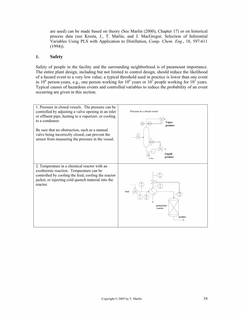
1. Safety Safety of people in the facility and the surrounding neighborhood is of paramount importance. The entire plant design, including but not limited to control design, should reduce the likelihood of a hazard event to a very low value; a typical threshold used in practice is lower than one event in 106 person-years, e.g., one person working for 106 years or 103 people working for 103 years. Typical causes of hazardous events and controlled variables to reduce the probability of an event occurring are given in this section. 1. Pressure in closed vessels. The pressure can be controlled by adjusting a valve opening in an inlet or effluent pipe, heating to a vaporizer, or cooling to a condenser. Be sure that no obstruction, such as a manual valve being incorrectly closed, can prevent the sensor from measuring the pressure in the vessel.

Vaporproduct

Liquidproduct

T6 PC1

LC1

A1

L. Key

Pressure in a closed vessel

2. Temperature in a chemical reactor with an exothermic reaction. Temperature can be controlled by cooling the feed, cooling the reactor jacket, or injecting cold quench material into the reactor.

feed

product

packed bedreactor

TC3

T2

F2

F1

T1

A2


3. Flows and composition in a system that can enter an explosive concentration. See Workshop 2 in the Short-cut design topic.

4. Levels when the material is hazardous 5. Pressures when the flow must be in a specific direction. An example is maintaining good hygiene, which can require that no air enter the system. The process must be maintained at a pressure above ambient.

Special Issues: 1. Alarms are addressed in objective seven. However, every safety-related variables should have an alarm that warns the operator before an unsafe value occurs. 2. A feedback loop can fail because it relies on a sensor, computation, and final element. Therefore, safety interlock systems (SIS) and pressure relief systems are included for safety-related objectives. 3. Safety of the product to consumers is covered in Product Quality.

2. Environmental Protection Process plants handle large quantities of material, so that if even a small percentage is hazardous, the effluents from a plant have the potential to cause harm to the environment outside of the manufacturing facility. Major reductions in hazardous emissions result from modifications to process chemistry and flowsheet structure. However, control contributes to the reduction of undesired effluents by monitoring and introducing corrective actions when needed. 1. The concentration in liquid streams can be monitored and actions can be taken based on the measured value. a. When a water-based stream has unacceptably high concentrations, it can be recycled to a holding pond for further processing before release. b. The pH of a stream can be controlled by addition of acid or base, as appropriate. c. The BOD of waste water treatment effluent can be measured and influenced by adjusting key


operating variables, for example, air flow to the biological reactors. 2. Emissions to the air can be undesirable as well. For example, incomplete combustion of fuel can create smoke; however, smoke (opacity) can be measured and nearly eliminated by achieving the desired excess air to a combustion process. We also note that having a deficiency of air in a combustion system can be hazardous. The uncombusted (or partially combusted) fuel can be mixed with air from a leak in the combustion chamber, away from the flame. An explosion can occur.

3. In some jurisdictions, flaring fuel is prohibited. A control system must control pressure by diverting fuel gas for immediate use in the process.

4. The Kyoto Protocol requires reductions in many effluents. One natural manner for reducing emissions is to increase the efficiency of existing processes. For example, a 1% increase in boiler efficiency, by improved control of excess air, results in a 1% reduction in CO2. Similarly, reductions in heating or cooling recycles, increased reactor yields to reduce feed flow and other improvements contribute directly to reduced effluents as well.

See the following WEB sites. http://www.ec.gc.ca/pdb/ghg/kyoto_protocol_e.cfm http://unfccc.int/2860.php

3. Equipment Protection Typically, process equipment is physically robust. However, operation outside of recommended regions of variables can lead to serious damage. The costs for equipment damage can be large, both in repair to the equipment and in lost production while the process is being repaired. Control systems are used to maintain acceptable values for key variables and if undesired regions occur due to upsets, to shutdown the equipment to prevent damage.


1. Flow is an important variable. a. Some pumps require a continuous flow, and no pump should be operated for a long time with no flow rate. Therefore, controls often ensure a continuous flow by opening a recycle when the net flow through the process is too low. b. Compressors are used for the flow of gases and in vapor compression refrigeration systems. Centrifugal compressors have required minimum flows; lower flows can lead to unstable flows, high frequency oscillations, and severe damage. Recycle flows are required to ensure the minimum flow is exceeded. c. Fired heaters usually require a minimum flow rate to prevent excessive heating of the tubes and decomposition of fluids in the pipes. d. Some chemical reactors require a minimum flow rate, for example, a packed bed to prevent excessive temperatures

b. Compressor with minimum flow anti-surge control

2. High temperature can damage even high quality steels. a. The maximum metal temperatures can be exceeded in fired heaters. They are measured with thermocouples welded to the pipes and by optical pyrometers. b. Special equipment can have limits on temperature and rate of change of temperature, for example, a glass lined, steel CSTR.

3. Pressure always has a range of acceptable values. a. Vessels with pressures above atmospheric are designed for a range, with the maximum never exceeded. b. We should also guard against low pressures, which can cause a vessel to collapse.

Coolingwater

Compressor

Motor

Frecycle

FC

Ffeed

Dump to safe locationDump to safe location

FC

LC

CW

fc

fo

fo

TPC

fo

Pressure relief valve


4. In some equipment, the level must be maintained to prevent damage. An example is a boiler, in which the flow of water from the drum to the tubes for heat exchange must be maintained at all times. This requires a sufficient water level in the drum.

5. Improper compositions can be harmful to equipment. a. Rapid corrosion can occur when an undesired composition occurs. One typical cause is liquid water in a hydrocarbon stream, which can corrode carbon steel. The water can be detected by a conductivity sensor, or the corrosion can be detected directly by a sensor. b. In some processes, very different compositions are required in selected equipment. For example, a softening resin is periodically regenerated using acid. A sensor should be installed to ensure that the acid never flows to integrated units that are not constructed to withstand the acid.

4. Smooth Operation Process plants are subject to continual disturbances in nearly all input streams. A well-designed control system should reduce the effects of these continuous disturbances on all important variables. In addition, the operations personnel appreciate a plant that operates smoothly, i.e., all trend plots show (nearly) straight lines. While the following objectives are not strictly required to achieve the higher priority objectives (or the lower priority either), good designs at this stage will improve the performance of controls for all other objectives. In addition, the controllers for this objective do not conflict with other controllers; because the controllers achieving smooth operation are generally lower in the control hierarchy and are directed by controllers for other objectives. The typical implementation approach involves the cascade control structure.

BFW

Superheated steam

air

Fuel gas

Natural circulation

Drum level


1. Control all unstable variables. An unstable variable will exceed desired values and lead to poor, if not dangerous, plant operation. Liquid levels in tanks with pumped effluent are unstable.

LC

Fin

Fout

Tank level with pump

1. The plant production rate should be determined by a single controller. a. Many other flows can be maintained in a ratio to the production flow rate. b. The production rate is typically located at the beginning or the end of the process. c. Only in unusual circumstances will the production controller adjust a flow rate that is neither the entering feed or leaving product. This can be done to provide a very smooth flow to a unit that is extremely sensitive to flow disturbances.

2. Plants contain inventory to allow short-term differences between unit flows in and out. a. Intermediate liquid levels in a plant are controlled to enable one controller to achieve production rate control. b. For Vapors, pressure control achieves a balance of flows in and out. c. For granular solids, the level or weight of a container can be controlled to achieve flow balancing.

3. Important properties of flows entering the process should be held constant. Typical properties are flow rate and temperature.

F0

LC LC LC

F1 F2 F3

“Feed push” with levels adjusting flows out

F0

LC LC LC

F1 F2 F3

“Product pull” with levels adjusting flows in

F0

LC LC LC

F1 F2 F3

“Feed push” with levels adjusting flows out

F0

LC LC LC

F1 F2 F3

“Product pull” with levels adjusting flows in


4. The “process environment” should be controlled in most units. a. In distillation towers, the feed flow rate, enthalpy and tower pressure are key variables. b. In a series of packed bed reactors, the pressure, feed flow rate, and bed inlet temperatures are key.

Pressure and temperature in a flash process.

Vaporproduct

Liquidproduct

T6 PC1

LC1

A1

L. Key

5. Many variables will tend to “drift” if not measured and controlled. For example, maintaining a valve at a constant % open will not ensure constant flow, because of disturbances in pressures and fluid density.

5. Product Quality Most processing plants desire to achieve strict quality specifications on the material produced. Usually, this is a product for sale, but it could be an effluent for release to the environment or a utility stream, such as steam, that will be used in an integrated plant. Since the purpose of the facility is to make the product, success depends on excellent quality control. Not all plants make a final product for sale; some plants make intermediate products that are used in subsequent steps to ultimately make a final product. Control of the intermediate products is also important, even if poor intermediate quality can be rectified in subsequent manufacturing steps, because these corrections usually involve increased cost and lower production capacity. 1. Product quality is related to its final use a. In some cases, qualities are directly related to a stream composition; thus, the selection of measured variable is obvious. For example, the quality of ethylene for use in polymerization is measured by impurities of components like acetylene, ethane and methane. b. In other cases, the performance must be measured directly, because it is a complex function of many material components. For example, • fuel properties are measured in test engines for

octane • tensile strength of fiber is tested


2. Depending on the sensor technology and need for rapid measurement, the variable can be measured in many ways. a. In Situ - A sensor is inserted in the process and measures the variable in the process. For example, this approach is used for temperature measurement using thermocouples, pH measurement, and pressure measurement. b. Onstream sample - When the process environment is too hostile for the sensor, a sample can be withdrawn and sent to the sensor. In this case, the sensor is located at the process unit, the sample is withdrawn automatically, and the measured value is transmitted automatically to the control computer for use in monitoring and control. c. Remote laboratory - When the analysis is very complex and expensive, a sample may be collected and transported to a laboratory. The measured value is reported when available and can be used for adjusting the process.

Analyzer feedback control using onstream measurements

3. To achieve desired product qualities, we generally adjust process environment variables based on process fundamentals and empirical data. Therefore, we must be sure to measure the key process environment variables.

4. Inferential variables - Often, measuring product quality is quite expensive and introduces significant delays in the measurement. Therefore, we seek “surrogate” or inferential variables that are strongly correlated to the product quality. Naturally, the inferential variables should be much easier to measure, i.e, a lower cost and fast measurement. An appropriate inferential variable depends upon the process. Some examples include • For reaction conversion, the temperature

difference across an adiabatic packed bed reactor • For distillation product composition, a tray

temperature • For BOD, COD • Stirrer power for liquid viscosity

Control of the temperature increase for an adiabatic chemical reactor with exothermic reaction

6. Profit For commercial endeavors, profit is required. In other facilities, such as waste water processing, no option exists to not operate the plant; however, profit maximization is equivalent to a cost minimization, and every plant benefits from achieving its goals at as low a cost as possible.

AC

AC

AC

AC

feed

product

heating stream

packed bedreactor

T4

T3

T2

F2

F1

T1

A2

TY3

dTC5

T4-T3

Set point is desired temperature rise across reactor


Maximizing the profit involves many engineering functions, such as feed purchasing, price negotiation, and process equipment design. Here, we will concentrate on the actions possible after the process flowsheet and equipment have been defined. We do not want to degrade the achievement of higher priority goals; therefore, the approaches presented here are usually implemented slowly, to prevent unfavorable interaction. 1. Often, the process can be analyzed offline, and the results of the analysis implemented as set points to feedback controllers. a. In combustion systems, achieving several hundred parts per million CO in the flue gas by adjusting the air flow to the burner is typically nearly optimal. b. The optimum tradeoff between distillation product purity and energy consumption in the reboiler and condenser can be estimated, and the product composition controlled to achieve the optimum. c. The trajectory of a key measured variable may define good operation in a batch process. It should be measured and controlled to the pre-calculated trajectory. d. The optimum can be defined by the proper ratio of flows. It should be measured and controlled to the pre-calculated value. • Ratio of dilution steam to hydrocarbon feed in

an olefins-producing pyrolysis reactor • Ratio of reflux to feed for a distillation tower

The optimum value of the product compositions depends on the values of the products (as the compositions change) and the energy required for separation.

Many times, the best operation is near a limitation or constraint in a specific variable. Control should maintain the variable near the constraint without violating the limit. Examples include • Minimum pressure in many distillation towers • Minimum anti-surge recycle around a

compressor • Maximizing production as limited by various

equipment capacities

The most profitable operation is at a high temperature, but temperatures beyond a maximum will damage the equipment.

AC

AC

AC

AC


3. Often, the plant contains more manipulated than controlled variables. Thus, the process has flexibility to achieve all controlled variables while reducing costs, since different manipulated variables can have different costs. • Make the total steam from several boilers at

the lowest fuel cost • Achieve the maximum heat recovery from

parallel heat exchangers • Compress gas to the desired pressure with a

minimum energy cost using parallel compressors

4. In some cases, the optimum operation changes frequently, depending on changes to variables such as feed composition, equipment performance, and production rate. An online calculation is performed to determine the optimum operation. The sensors required depend on the calculations and on which variables change significantly. • Optimal blending of hydrocarbons to produce

gasoline • Optimum operation of parallel refrigeration

units to provide cooling to a process. • Optimum operation of parallel reactors whose

yields change over time.

Gasoline blending is controlled and optimized in closed-loop

Reformate

LSR Naphtha

N-Butane

FCC Gas

Alkylate

Final BlendFT

AT

FC

FC

FC

FC

FC

Flow setpoints

Flows

Blend Octane

BlendRVP

Measured

+

-

Predicted

BiasLP


7. Monitoring and Diagnosis Typically, a plant contains many sensors that are not used for closed-loop control; in fact, more sensors are normally installed for monitoring and diagnosis than for feedback control. In general, the sensors provide considerable information, but no one sensor provides a unique indication that a specific problem has occurred, or is likely to occur in the near future. Thus, some diagnosis is required and this diagnosis involves people applying problem-solving techniques. In general, there are two distinct categories of monitoring and diagnosis. The first category involves issues that occur relatively rapidly and must be corrected quickly to prevent a hazard, equipment damage or large economic loss. The plant personnel near the equipment, i.e., the plant operators, will perform these rapid diagnostics and implement corrective actions. When actions are required quickly, an alarm can be generated using the measured value. An alarm activates a blinking light and an audio signal to the operator. After the operator acknowledges the alarm, the audio signal is stopped and the light associated with the alarm variable remains on (without blinking) until the variable returns to its acceptable range. The second category involves slower changes that can be monitored periodically. Often, engineers perform the diagnosis and plan the corrective action, because the correction can involve temporarily taking a unit out of service for repair, catalyst regeneration, or cleaning. Typically, daily reports are generated that summarize the performance of all key units. The reports can contain values of measured variables, calculated values that summarize equipment performance (e.g., heat transfer coefficients) and values that summarize process performance (e.g., yields, energy/feed, etc.). One important calculation involves material balances on the process. 1. High priority alarms require immediate action by plant personnel. The variable should be measured by a sensor that is separate from the control system, i.e., a redundant sensor should be used.

2. A medium priority alarm indicates a situation that should be monitored closely. Whether a separate sensor is required depends on the consequence of the situation.

A low level could damage the pump; a high level could allow liquid in the vapor line.

The pressure affects safety, add a high alarm

F1

PAH

LAHLAL

Too much light key could result in a large economic loss

AAH


3. Many sensors are provided to the centralized control room for monitoring the process environment. Some examples are • Temperatures on several trays in a distillation

column • Pressure profile in a column with packing or

trays • Temperatures and pressures in refrigeration

cycle. Note that the pressures and temperatures are related for the boiling/condensing refrigerant.

5. Redundant sensors are provided for very critical measurements, which enables people to identify a sensor malfunction.

6. Some sensors are provided with local displays so that operators performing tasks at the equipment (start up, maintenance, etc.) can monitor values.

7. Sensors can be provided to calculate equipment and performance calculations.

FC

LC

CW

TC

fc

fo

fo

L LAHLAL

TAH

T T

TY>

PC

fo

PAH



Workshop 1B. Guidelines for Selecting Manipulated Variables Most manipulated variables in the process industries are easily identified and naturally provided in the process design. However, the principles of strong, precise, and fast feedback action, along with high profit, leads to some special designs. A few general issues are discussed in the following. a. Remote actuation - Most processes are managed from a remote, centralized control room, where most personnel and the control computing equipment are located. If the response of the feedback must be implemented rapidly and reliably, the final element must be adjustable from the control room. This is nearly always the case for automatic control. Some final elements are changed very infrequently, for example, a valve that determines the source of feed material from several storage tanks; a person could adjust these valves manually. b. Strong effect - This is essentially a “large steady-state gain”. We can determine the gain from the product of the gain between the adjusted variable (usually flow rate) and the controlled variable and the gain between the controller output and the adjusted variable. Typically the gain should be in the range of 1 (% controlled variable)/(%controller output). Note that in this equation, the range of the controlled variable should be the typical range over which control is applied. If the gain is too small, the control system cannot correct for large disturbances or achieve a range of desired set points. c. Good Precision - The manipulated variable should achieve “close” to the value commanded by the controller. Naturally, an exact implementation is not achievable, and the meaning of “close” varies depending on the process application. When the final element is a control valve, friction impedes the movement of the valve and can lead to dead band and hysteresis. In addition, a valve with a large maximum flow rate (i.e., a larger valve”) generally has poorer precision. d. Fast response - Feedback performance is better for fast dynamics between the final element and the controlled variable (sensor). This is an important factor in deciding which final element to adjust for feedback of a specific controlled variable. e. Linear process dynamics - The typical feedback controller is linear, with constant tuning parameters. This controller will function best when the process is also linear, so that the closed-loop behavior of the system is relatively constant over the range of operation. f. High profit - In some cases, the cost for manipulating one final element may be different fro a similar final element. For example, using a hot process stream for reboiling may have not net cost, if the stream must be cooled for subsequent processing. The alternative of using steam from a fired boiler is much more costly, as fuel is required in the boiler.



Workshop 1C. Is the Desired Control Performance Achievable?

This issue is addressed in the topics of controllability and optimization-based control design. The approaches using linear dynamic models will not be repeated here. However, a steady-state flowsheet can be helpful for processes that normally operate at steady state. The advantage for using a flowsheeting simulation is the natural inclusion of non-linear behavior. In addition, commercial steady-state flowsheets are widely available, low cost and easily used. Non-linear behavior is important as the operation deviates form the point of linearization. Thus, the flowsheet gives a better indication of the range of achievable behavior, albeit in the steady state. Often, the simulator is used to determine the largest disturbance that can be compensated with the equipment in the design. The disturbance can be increased until one (or more) manipulated variable reaches a bound (e.g., maximum reflux flow rate) or another equipment limitation is encountered (e.g., maximum vapor flow rate in a section of a distillation tower).



Workshop 1D. Eliminate Unacceptable Loop Pairings? In most design procedures, we eliminate many unacceptable designs using limited data and simple calculations or rules. This enables us to consider a problem with many potential solutions and to concentrate the available time and resources on evaluating the most promising designs in greater detail. While we seek to narrow our search quickly, we must be cautious. When we use simple calculations and guidelines, we limit our solution of “conventional” designs. This limitation may be acceptable in some cases, but we could miss opportunities for substantial improvement in some cases. Here, we will concentrate on process insight, guidelines and simple calculations for design. We will accept the possibility of missing a very good design; however, the section on optimization-based control design addresses a more thorough screening procedure that should converge to all good candidates. Before presenting these guidelines, we offer a caution: the guidelines are often violated in practical control. The solutions to the design cases in this lesson provide many examples. This situation results from the multi-objective nature of the design problem. The highest priority objective can change, depending on the situation. Therefore, guidelines always have the caveat, “With all other considerations equal”. With the preceding caution in mind, we present a few steps that can be used to test candidates. a. Is performance achievable? - For short-cut analysis, we will concentrate of steady-state

behavior.

i. The number manipulated variables must be equal to or greater than the number of controlled variables.

ii. The linear gain matrix must be invertible, i.e., its determinant must exist. (Other tests are available and can be used in the optimization-based approach; here, we concentrate on simple calculations.)

iii. The largest expected disturbances must be compensated by the manipulated variables, as evaluated using a steady-state flowsheet.

b. Favorable dynamics - The basics of feedback support the following guidelines. i. The feedback dynamics should be fast, especially the dead times. ii. Disturbances should pass through processes with large time constants.

iii. Disturbances should occur at frequencies much larger than the critical frequencies of the feedback loop.

iv. Inventories should be large enough to attenuate changes in flows to critical units.

c. Achieve integrity – We use steady-state gain information at this step.

i. Avoid control designs with loop pairings on negative relative gain elements. ii. Avoid control designs with loop pairings on zero relative gain elements


iii. If a design has a loop paired on a negative or zero RGA element, an “interlock” should be implemented to ensure that appropriate loops are “off” simultaneously to retain stability.

d. Interaction and performance – Select designs with modest and favorable interaction, f

possible. i. Avoid designs with loop pairings on very small positive (e.g., 0.15) elements. Very

small elements indicate a much larger effective process gain in the multiloop system, which will require retuning the controllers as loops change from on to off.

ii. Avoid designs with loop pairings on very large RGA elements. Large elements indicate a much smaller gain in the multiloop system, which usually cannot be compensated by a large controller gain because of stability.

iii. Select designs with favorable interaction for key disturbances. This can be determined using the RDG.

e. Minimize effects of disturbances – Some disturbances are inevitable, os that their

effects should be minimized.

i. Control the “process environment”, as measured by inexpensive, fast and reliable sensors. By controlling these variables, the deviations of critical variables, such as product qualities are reduced. This concept is referred to using two terms; inferential control or partial control.

ii. Where an appropriate secondary variable exists, apply cascade control to reduce the effects of some disturbances.

iii. Where an appropriate sensor for a disturbance exists, apply feedforward control to reduce the effects of some disturbances.

iv. Apply averaging level control where appropriate to reduce the effects of changing flow rates.



Class Workshop: Design controls for the Butane vaporizer which is the first unit in a Maleic Anhydride process.

Periodic feed delivery

Short-cut Control Design Workshop 2

L2

P2

Short-cut Control Design Workshop 2Some useful information about the plant. 1. Essentially pure butane is delivered to the plant periodically via rail car. 2. Butane is stored under pressure. 3. The "feed preparation" unit is highlighted in the figure. The goal is to vaporize the appropriate

amount of butane and mix it with air. After the feed preparation, the mixed feed flows to a packed bed reactor; effluent from the reactor is processed in separation units, which are not shown in detail.

4. Heat is provided by condensing steam in the vaporizer. 5. Air is compressed by a compressor that is driven by a steam turbine. 6. There is an explosion limit for the air/C4 ratio. Normal is 1.6% butane, and the explosive range is

1.8% to 8.0% You are asked to design a control system for the process in the dashed box. You should a. Briefly, list the control objectives for the seven categories. b. Add sensors and valves needed for good control. c. Sketch the loop pairing on the figure. d. Provide a brief explanation for your design. e. If you feel especially keen, include "control for safety" in your design. This would include the

following items (among others). - alarms - safety shutdown systems - pressure relief - failure position for valves

Short-cut Control Design Workshop 2Table 1. Control objectives

Control Objective

1. Safety

• Control pressure in vaporizer • Control pressure in reactor and downstream vessels • Prevent explosive composition in the reactor feed

• Environmental protection

• Send any vent gas with hydrocarbons to flare for combustion

• Equipment protection

• Ensure air flow to compressor • See safety above.

• Smooth operation

• Control the liquid level in the vaporizer because it is open-loop unstable • Control the feed/production rate with the air flow rate to mixing point Adjust the steam flow to achieve the desired vaporizer pressure and reduce disturbances to the butane flow

• Product quality

• Profit • Monitoring and

Diagnosis

• Monitor pressure drop across the packed bed reactors • Compare the butane temperature and pressure to check the pressure sensor • Compare the ratio of steam/butane to check for steam losses via leaks. • Compare butane/air ratio as a check on the analyzer

The key vaporizer variable is pressure, because of safety issues due to material limits of the steel. Note that the temperatures are low, so that the temperature is not a limiting factor. Because the feed is a pure component and is boiling in the vaporizer, the temperature and pressure are related; only one can be specified independently! Therefore, both cannot be controlled with feedback controllers. The pressure is important and the pressure sensor is fast; therefore, we control pressure. Since the pressure response is as fast as the temperature response, a cascade design (PC→TC→v2) is NOT appropriate.




Periodic feed delivery

L2


Valve Failure position Valve positioner recommended?

v1 Closed – prevent liquid carryover to reactor. May have to have recirculation line from pump back to storage.

No, because tight level control is not required and loop has no dead time.

v2 Closed – lower pressure in vaporizer vessel.

Yes, because tight pressure control is important and dynamics could be a couple of minutes (heating the coils).

v3 Closed – Safe low concentration of butane in reactor feed. Note that this closes outlet to the vessel; therefore, safety relief valves must prevent high pressure.

No, if the loop is fast. Yes, if the loop is slow compared with the safety issues.

v4 Open – Dilute the butane with air to yield low (safe) concentration. This also protects compressor from running without air flow.

No, because the loop is fast. Yes, if the valve has strong unbalanced forces or sticking.

v5 Open – lower pressure No, loop is fast



Class Workshop: Design controls for the fuel gas distribution system.


The gas distribution process in the figure provides fuel to the process units. Several processes in the plant generate excess gas, and this control strategy is not allowed to interfere with these units. Also, several processes consume gas, and the rate of consumption of only one of the processes can be manipulated by the control system. The flows from producers and to consumers can change rapidly. Extra sources are provided by the purchase of fuel gas and vaporizer, and an extra consumer is provided by the flare. The relative dynamics, costs and range of manipulation are summarized in the following table.

flow manipulated dynamics range (% of total flow) cost

producing no fast 0-100% n/a

consuming only one flow fast 0-20% very low

generation yes ? 0-100% low

purchase yes ? 0-100% medium

disposal yes ? 0-100% high

a. Complete the blank entries in the table based on engineering judgement for the processes

in the figure. b. Complete a Control Design Form for the problem. Specifically, define the dynamic and

economic requirements. Hint: To assist in defining the proper behavior, plot all fuel gas flows vs. (consumption -

production) on the x-axis. c. Design a multiloop control strategy to satisfy the objectives. You may add sensors as

required but make no other changes. d. Suggest process change(s) to improve the performance of the system.


Fuel gas header pressure control - The pressure of the fuel gas header is a crucial variable for theentire plant because many units produce or consume the gas and disturbance in the header can affectmany units simultaneously.

The completion of the table is

generation slowpurchase fastdisposal fast

The control design should be constructed to control pressure tightly while operating the system isan efficient manner. Efficiency is achieved by 1) purchasing only when necessary, 2) disposing onlywhen necessary, and 3) vaporizing only when necessary.

Two solutions using the split range concept are presented because many valves are adjusted tocontrol a single variable. Since four valves are manipulated, the split range approach is modified toprevent a four-way split; no more than a two-way split is used. The selection between the two solutionswould depend on plant experience on the speed of response of the vaporizer for typical disturbances.

Solution I assumes that the vaporizer dynamics are fast enough to tightly control pressure. In thisdesign, the normal pressure controller is a split range which adjusts the consuming and fuel vaporizationvalves. For large upsets, a single pressure controller adjusts the disposal valve; to prevent competitionwith the normal controller, this controller has a set point that is slightly higher than the desired pressure. Thus, this controller only opens the disposal valve when the pressure is (slightly) elevated. Also, a singlecontroller adjusts the purchase valve; to prevent competition, this controller has a set point which isslightly lower than the desired pressure. These two controller implement extreme, but necessary, actionswhen the pressure deviates significantly from the desired value.

Solution II assumes that the vaporizer dynamics are too slow for control of the header pressure. The normal pressure controller is a split range which adjusts the consuming fuel and the purchase valves;both of these provide extremely fast dynamic responses. For large upsets, a single pressure controlleradjusts the disposal valve; to prevent competition with the normal controller, this controller has a set pointthat is slightly higher than the desired pressure. Thus, this controller only opens the disposal valve whenthe pressure is (slightly) elevated. To reduce the expense fuel purchase, a valve position controller isprovided to slowly reduce the purchasing (when it exists) by vaporizing the less expense liquid fuel.




Solution I


Short-cut Control Design Workshop 3Solution II



Class Workshop: Design controls for the refrigeration system.


Refrigeration is very important for industrial processes and our daily comfort in the summer. In industry, it is used to provide cooling when the temperatures are below the temperature of cooling water. The controlled objective could be a temperature (heat exchanger), a pressure (condenser) or any other variable that could be influenced by heat transfer. Refrigeration can consume large amounts of energy for the heat transfer, especially at low temperatures. Thus, the control system should provide the desired control performance at the lowest energy input possible. Before designing the controllers for this exercise, you might need to quickly review the principles of vapor recompression refrigeration. This exercise involves the simple, single stage refrigeration circuit in Figure 1. A. Develop a regulatory control design for this system which satisfies the demands of the

consumers. Two consumers are shown as a heat exchanger (T3) and a condenser (P2); naturally, many others could exist. Part of your design should provide control for the twoconsumers shown in the figure. Provide a brief explanation for each controller.

B. Add necessary controls to minimize the energy consumption to the turbine while

satisfying the consumers' demands. Explain your design. In both parts of this question you may add sensors and add and delete valves.



Refrigeration circuit - This single-stage refrigeration process has most of the elements of a morecomplex multistage process.

a. Generally, a refrigeration system is provided to satisfy the varying demands of process consumers. Controllers to satisfy the consumers adjust the flow of liquid refrigerant to heat exchangers where therefrigerant vaporizes as heat is transferred. In Figure a, the temperature and pressure controllers usesingle-loop PI controllers to adjust the flows of the appropriate liquid refrigerant.

b. The design in a above could be quite inefficient. The first step would be to remove unnecessary valveswhich create pressure drops that would increase energy consumption. The eliminated valves are circled.

The next step is to maximize the cooling water which will reduce the exhaust pressure, again reducingenergy consumption. Finally, the power to the compressor should be just enough to satisfy the process, orstated another way, the refrigerant should be just cold enough to satisfy the process requirements. Theprocess requirements are indicated by the liquid refrigerant valves to the consumers. The most openvalve should be (slightly) below 100% to allow the controller to respond to higher frequencydisturbances. This is determined by a signal select and valve position controller. The valve positioncontroller adjusts the compressor speed, which is cascaded to the steam flow (power source). Thecompleted design is shown in Figure b.



Short-cut Control Design Workshop 4Solution A

Short-cut Control Design Workshop 4Solution B



Class Workshop: Design controls for the flash process.

Feed


Vaporproduct

Liquidproduct

Processfluid

Steam

F1

F2 F3

T1 T2

T3

T5

T4

T6 P1

L1

A1L. Key

P ≈ 1000 kPa

T ≈ 298 K


v1

v3

v5

v4

−−−−−

−−−−−

=

54321

0265.179.31.136.0113.36.5039.180.6567.

043.044.11.00917.19.044.85.0708.000.200

/1161

1 vvvvv

dtdLPATF

1. Safety- Maintain vessel pressure below 1200 kPa

2. Environmental protection- Prevent release of hydrocarbons to the atmosphere

3. Equipment protection- Ensure that liquid flows through the pump

4. Smooth operation- When possible, make slow adjustments to liquid product product flow rate

5. Product quality- Maintain the liquid product at 10 ± 1 mole% L. Key.

6. Profit- Minimize the use of the expensive steam for heating

7. Monitoring and diagnosis- Provide alarms for immediate attention by operating personnel

Here is the process gain

matrix calculated at the nominal operation.


• Can we control these with the valvesshown, i.e., is the system controllable?

Let’s select:

F1 production rate

T6 feed vaporization

A1 product quality

P safety

L liquid to pump

−−−−−

−−−−−

=

54321

0265.179.31.136.0113.36.5039.180.6567.

043.044.11.00917.19.044.85.0708.000.200

/1161

vvvvv

dtdLPATF

The effects of v1 and v2 are identical, within a constant. Therefore, the five CVs cannot be independently affected by the five valves.

Det [KP] = 10-7


Not Controllable!×12




• Can we control these with the valvesshown, i.e., is the system controllable?

Let’s select:

F1 production rate

T6 feed vaporization

A1 product quality

P safety

L liquid to pump

The effects of v1 and v2 are identical, within a constant. Therefore, the five CVs cannot be independently affected by the five valves.

T6v2

v1

T2

A1

P1

sL1

Both v1 and v2 affect CVs of interest through T6. This is a contraction that reduces the controllability.

Not Controllable!


−−−−

−−=

5432

0265.179.31.136.36.5039.180.6

043.044.11.

000.20

/11

1

vvvv

dtdLPA

F

The effects of v1 and v2 are identical, within a constant. Here, we remove v1 (arbitrarily).

Det [KP] = 10-1 ≠ 0

Yes, controllable!

0100/183.10083.183.0083.11001015432

dtdLPAF

vvvv

−−

RGA

The pairings with positive RGA elements also have good dynamics and range




Our process insight indicated that T6 is an important variable. However, we recognized that P1, A1 and T6 cannot be controlled independently. Should we ignore T6?

No! The temperature is an important part of the process environment, and it can be measured quickly and at low cost. Our process insight indicates that the temperature provides an indication of the composition.

Thus, T6 is a good “inferential” or “partial control” variable. It can be controlled and reset by AC-1 in a cascade structure.


Feed


Vaporproduct

Liquidproduct

Processfluid

Steam

FC-1

F2 F3

T1 T2

T3

T5

TC-6 PC-1

LC-1

AC-1

L. Key

Split range PAH

LALLAH

cascade



Class Workshop: Design controls for the CSTR with recycle.

v1

Hot Oil

v2

v3

L1

v7

v5 v6

Hot Oil

F1 T1 T3

T2

F2

T4T5

F3 T6

T8

F4

L2

v8

T7

P1F5

F6T9

Feed

Product

Periodic feed delivery to storage tank


Adiabatic CSTR

Unreacted feed with trace product

Flash separator

v4

A2

TITLE: Chemical reactor |ORGANIZATION: McMaster Chemical EngineeringPROCESS UNIT: Hamilton chemical plant |DESIGNER: I. M. LearningDRAWING : Figure 25-8 |ORIGINAL DATE: January 1, 1994 |REVISION No. 1 CONTROL OBJECTIVES:1) SAFETY OF PERSONNEL

a) the maximum pressure in the flash drum must not be exceeded under any circumstancesb) no material should overflow the reactor vessel

2) ENVIRONMENTAL PROTECTIONa) none

3) EQUIPMENT PROTECTIONa) none

4) SMOOTH, EASY OPERATIONa) the production rate, F5, need not be controlled exactly constant; its instantaneousvalue may deviate by 1 unit from its desired value for periods of up to 20 minutes. Itshourly average should be close to its desired value, and the daily feed rate should be setto satisfy a daily total production target.b) the interaction of fresh and recycle feed should be minimized

5) PRODUCT QUALITYa) the vapor product should be controlled at 10 mole% A, with deviations of ±0.7% allowedfor periods of up to 10 minutes.

6) EFFICIENCY AND OPTIMIZATIONa) the required equipment capacities should not be excessive

7) MONITORING AND DIAGNOSISa) sensors and displays needed to monitor the normal and upset conditions of the unit mustbe provided to the plant operatorb) sensors and calculated variables required to monitor the product quality and thermalefficiency of the unit should be provided for longer term monitoring

DISTURBANCES:

SOURCE MAGNITUDE PERIOD MEASURED?

1) impurity in feed day no (Influences the reaction rate, basically affecting the frequency factor, k0.)2) hot oil temperature ± 20EC 200+ min yes (T2)3) hot oil temperature ± 20EC 200+ min yes (T8)4) feed rate ±1, step shift-day yes (F1)



Short-Cut Design Procedures Workshop 6 The following is a brief consideration of the first four levels of the temporal decomposition for the CSTR with recycle design problem. Level 1 - flow and inventory i) The feed tanks have periodic deliveries of material and continuous outflow to the process.

Therefore, it is not possible or necessary to control the level. The tanks must be large enough so that they neither overflow nor go empty for expected delivery and outflow policies.

ii) The feed to the reactor is a combination of fresh feed and recycle. The flow and inventory design must consider this factor to prevent oscillations caused by interactions. Also, there seem to be several possible ways to control the flow to the reactor since there are valves in the fresh feed, recycle flow and combined flow.

iii) There is no option for the disposition of the reactor effluent; it must proceed directly to the flash drum.

iv) The vapor product comes from a small drum inventory and flow fluctuations can be expected. Since the control objectives allow for variability in the product rate, this is not likely to be a concern.

v) Two liquid levels are non-self-regulatory and should be controlled via feedback to prevent them from exceeding their limits. Also, one vapor space pressure, while theoretically self-regulating, can quickly exceed the acceptable pressure of the equipment; therefore, the pressure should also be controlled.

Level 2 - process environment vi) Several manipulated variables (v1, v2, v3, v4, v7) and all disturbances affect the reactor

temperature and reaction rate. Level 3 - product quality vii) There appear to be several manipulated variables that affect the flash product quality, A2. Level 4 - profit viii) There are no objectives specified to increase profit beyond controlling product flow rate

and quality. However, there appear to be extra manipulated variables, or at least extra valves in the process. This inconsistency must be resolved.

Since no severe difficulties were identified in the third step, we proceed to the fourth step where we begin to design the control structure. Since we anticipate strong interaction among variables due to the process recycle, process decomposition is not applied. However, the control is designed according to the five-level temporal hierarchy. The overall structure is first selected; then, enhancements are added; finally, algorithms and modes are chosen. Level 1 - flow and inventory The first decision is usually the flow controller which determines the throughput in the process. Usually, this controls either the feed rate or the production rate. The control objectives state that


the production rate does not have to be maintained invariant, which is fortunate since controlling the vapor flow from a flash drum would be difficult without allowing the pressure to vary excessively. For this process and objectives, the feed rate, F1, will be controlled. Any of three valves, v1, v3, or v4, could be adjusted to control F1. From the overview, it is realized that the v4 may be adjusted to control the liquid level control in the flash drum, so this is eliminated from consideration as a manipulated variable for controlling F1. Either of the remaining valves may be adjusted to control F2. Somewhat arbitrarily, we will select v1 as the manipulated variable; this selection has the minor advantage that the fresh feed can be reduced to zero and the system can be operated on total recycle for a short time. The remaining valve v3 is not needed and could be removed; in the example, we will simply maintain the valve position constant at its base case value. The reactor level must be controlled since it is non-self-regulating and the residence time affects the chemical reaction. The outlet flow is manipulated to control the level because the inlet flow has already been selected as the feed flow controller. The outlet flow is affected by both valves v5 and v6; thus, there are one controlled and two manipulated variables. We shall select valve v6 to maintain the highest pressure in the heat exchanger which tends to prevent vaporization. The redundant valve, v5, will not be adjusted. The liquid level in the flash must also be controlled within limits, and no objective compels tight or averaging control. Tight level control is selected since the level control is part of the recycle process and the entire process would not attain steady-state operation until the level attains steady state. The valve v4 was allocated to control the level when the feed flow was designed. The final issue at this level of the hierarchy is the pressure control of the flash drum. The vapor valve, v8, is selected to give fast control of pressure. In summary, the following allocation of controlled and manipulated variables have been made at this point.

controlled manipulated F1 v1 L1 v6 L2 v4 P1 v8

Levels 2 - process environment The reactor environment is affected by the flow rates and temperatures of the incoming streams. The fresh feed flow rate was specified to satisfy objectives at Level 1 of the hierarchy, but the total flow rate, F2, and the inlet temperature, T4, are available for reactor control, unless we chose to iterate and change the earlier decision. Of these two variables, only the inlet temperature, T4, is directly influenced by the manipulated valve, v2, although the total flow may be (and is) influenced through the recycle. The valve v7 would affect the reactor inlet temperature, but the dynamics would be slow because of the dynamics in the flash liquid inventory. Also, we can look ahead to the need to control the flash temperature, where v7 would give fast dynamics. Thus, we chose to adjust v2 to control reactor environment.


Level 3 - product quality The flash composition is to be controlled because it is the key measure of product quality, and it is controlled directly, without a temperature cascade, because the composition sensor is continuous with fast dynamics. The proper choice for the manipulated variable would be the heating oil valve v7 since it gives fast feedback dynamics over a large range of operation. In summary, the following allocation of controlled and manipulated variables have been made at levels 2 and 3.

controlled manipulated reactor v2 A2 v7

A reactor variable to be controlled has not yet been selected and could be temperature or concentration. Two alternative designs will be evaluated, temperature control and reactor concentration control. Level 4 - optimization There are no optimization objectives in the Control Design Form. The control design to this point has allocated all manipulated variables, except for v3 and v6 that were found to be redundant for the previous control objectives. These valves provide no additional process flexibility, except that of controlling some intermediate pressures in liquid flow lines. There seems to be no reason to control these pressures, and ordinarily, these valves would normally be eliminated to save equipment and pumping costs. In this case, the valves will simply be retained at their base case percent opening. To complete this step, enhancements to the basic structure of controller pairings is considered. For this simple process, the enhancements will be restricted to cascade and feedforward, and each controlled variable is discussed individually. F1 - The flow process is very fast, and the control design needs no enhancement. A PI

controller is appropriate for this process with nearly no dead time and significant high frequency noise.

L1 - The process has little or no dead time, and the pump pressure is relatively constant.

Thus, no cascade or feedforward is required, although a level-flow cascade may be used. The algorithm selected is a PI with tight tuning because the level influences the residence time, and zero steady-state offset is desired.

L2 - The process has little or no dead time, and the pump pressure is relatively constant.

Thus, no cascade or feedforward is required, although a level-flow cascade may be used. The algorithm is a PI with tight level tuning.

P1 - The process is fast, and the pressure should be maintained at its set point since it affects

the flash product compositions. Therefore, a PI controller is selected. A2 - The concentration of A in the product stream is the key product quality and is affected by

the disturbance in T8. Note that a cascade is not possible because there is no causal relationship between the valve v7 and the measured variable T8. A feedforward


controller is possible because the criteria for feedforward would be satisfied. However, as a preliminary decision, no enhancement will be selected because of the relatively fast feedback dynamics. This decision will be evaluated at the completion of this study. The feedback controller should have a PI or PID algorithm depending on the dynamics, fraction dead time, and measurement noise.

Finally, the reactor environment control options are evaluated to determine the best control design. Each is discussed briefly below. Design I - Figure 25-7 T5 - The reactor temperature is affected by several disturbances. These disturbances influence other measured variables before the reactor temperature measurement responds; thus, the potential for enhancements exists. For example, the measured fresh feed temperature, T3, could be a feedforward variable and the feed temperature T3 could be a secondary cascade variable. As a preliminary decision, the single-loop design T56 v2 is chosen with a PI algorithm. The resulting control of F1, T5 and A2 is controllable, as can be verified using the gains in equation (25-2) Design II - Figure 25-8 A1 - A more direct measure of the reactor operation is the concentration of A, which can be

controlled by adjusting valve v2, although with slow dynamics. Therefore, the cascade design A16T46v2 is selected, which gives good responses to temperature disturbances. The resulting control of F1, A1, and A2 is controllable, as can be verified using the gains in equation (25-2).

Level 5 – Monitoring All processes should be monitored for short term operation and longer term performance diagnostics. Shorter term issues involve alarms for critical variables, like the liquid levels and the flash drum pressure. Some of the longer term issues involve the reaction rate which is influenced by impurities in the feed; recognition of poor feed characteristics would enable the engineer to trace the cause of the poor feed and take actions to prevent recurrence of such conditions. To monitor the product rate, the flow measurement F5 should be accurate. If the density of the stream changes significantly, the conversion of sensor signal to the flow rate should be corrected based on a real-time sensor or laboratory data of density. Another monitoring goal would involve the performance of the heat exchangers, which might foul over time. The measurements of the flows, temperatures and valve positions enable some monitoring; for example, if the hot oil valve position increases over time at relatively constant production rate, the heat exchanger is most likely fouling. The lack of hot oil flow measurements prevents a complete check on the data; thus, the addition of flow and temperature sensors might be appropriate so that heat transfer coefficients can be calculated. Designs I and II are now complete. To evaluate their performances and select a final design, the dynamic performance of the process with each design was determined. In both cases, the process begins at the same initial steady state and is subjected to a change in feed impurity which reduces the reaction rate (frequency factor) to 90% of its base case value. The response of Design I is


shown in Figure 25-9. The operation of the process, especially the recycle flow rates, changes dramatically. The reason for this large change can be understood from process principles. The feed flow and the product purity remain unchanged. Therefore, the rate of production of B, Vk0e-

E/RTCA, must return to its initial value when steady state is attained. Since the reactor temperature and volume are maintained at their constant set points (in the steady-state) the concentration of the reactant must increase to compensate for the impurity. Because of the low "single-pass" conversion in the reactor, a large recycle flow rate change accompanies the change in concentration. For successful operation, the process equipment, pumps, pipes and valves, would have to have to have very large capacities, and thus, the plant design would be costly. The response of Design II is shown in Figure 25-10. After a transient, the process returns to nearly the same operating conditions, with the reactor concentration and volume at their initial values. To return the concentration to its set point, the A1 controller increased the reactor temperature, thus maintaining the production rate of B constant. This response returns to steady-state faster, satisfies all performance objectives for F5 and A2, and would not require excessive equipment capacity. Control Design II should be evaluated for all disturbances in the CDF; these others are discussed briefly here but not plotted. It performs well for the +20EC disturbance in T2, with only very small deviations in the compositions and product flow. The system experiences a rather large, but brief, disturbance when T8 increases in a step of 20EC. The maximum allowable short term variations in the product flow, F5, and the product composition, A2, are reached or slightly exceeded. If plant experience indicated that this disturbance occurred frequently, a feedforward compensation for changes in T8 adjusting v7 could be added to Design II. Finally, the response of a change in desired production rate, F5, is rather sluggish, since the feed flow rate is manipulated manually, and the product increases slowly as the recycle system responds, finally attaining steady-state. This is a direct result of the problem definition, since short term variation in the product rate was stated to have negligible influence on the process performance in the CDF.

The IAE for the product quality variable (A2) is 7.11 for Design I and 6.62 for Design II. Since Design II has good performance for the key quality variable, has well behaved dynamics for all variables, satisfies the control objectives, and requires equipment with smaller capacities, it is selected as the better control design for this process.



Design I


Design I

Disturbance is impurity that reduces the reaction rate by 10%.

Snow ball effect

Performance OK

Why did this occur?



Design II


Design II

Disturbance is impurity that reduces the reaction rate by 10%.

No snow ball effect

Performance OK

Why did this occur?



LC FC

fc

fc

fc

heatingcooling

from unit 1

to

unit 2

storage tank

v100

v110 v200

Class Workshop: Design controls tank with by-pass.


Control objectives:

1. Control the level in the bottom of the Unit 1 tower2. Control the flow rate to Unit 23. Cool any flow to the tank, which has an upper limit for

material stored4. Reheat any material from the tank to Unit 2, which

requires heated feed5. Minimize the heating and cooling

Disturbances:

The flows from Unit 1 and to Unit 2 cannot be adjusted by this control system. They are typically not equal, and either can be larger at a specific time.




This example demonstrates how split range and signal select can be combined in control designs toachieve good control performance. A more efficient alternative approach would be to provide themaximum allowable direct flow from unit 1 to unit 2. The maximum direct flow between units would belimited by either the availability from unit 1 or the demand for unit 2, with the limiting conditionchanging as unit operations changed. A control system to automatically maximize the direct flow whilealways achieving proper level and flow control would be desirable. Such a system is shown in Figure 22-11, where both the level and flow controllers have split range outputs. Both controller outputs are send tothe low signal select which determines the proper signal to manipulate the direct flow valve, which in thisexample is the smallest signal (resulting in the smallest flow rate). Thus, one controller will adjust thedirect flow valve, and the other controller will continue to increase its output until it adjusts the flow tothe tank (for level control) or flow from the tank (for flow control), as appropriate. The resulting designis given in Figure a, and the operations for the two situations are summarized below.

how each valve is adjustedrelative flows v100 v110 v200 net flow

unit 1 flow > unit 2 flow by FC by LC closed to storageunit 1 flow < unit 2 flow by LC closed by FC from storage

With this control system, the plant personnel need only input the set points to the level controller(normally 50% of range) and the flow controller (required flow to unit 2). The system automaticallyadjusts the valves as described to meet the level and flow requirements while minimizing flows to andfrom storage, thus minimizing energy use.





Class Workshop: Design controls for a decanter.


Control Objectives:1. Pressure in the vessel2. Interface level in the vessel3. Flow rate(s) How many can be controlled independently?

Disturbances:The following additional information is provided about the variability of the process operation; the feed flow is 1400-2600, the percent overhead in feed is 1-5%, and the pressures are essentially constant.

Process information:You may assume that the flows are proportional to the square root of the pressure drop and the valve % open; the valves are all 50% open at the base case conditions.


Short-cut Control Design Workshop 8However In the process, a change in the flow into the vessel requires an immediate change in the flow outbecause the inventory is (essentially) incompressible. Thus, the pressure controller must adjust a valvewith a range large enough to respond to the change of feed rate. Valve 2 is much too small for thispurpose, while valve 3 is large enough. The liquid level controller adjusts for changes in the ratio of lightto heavy material in the feed, which can be accomplished by adjusting valve 2.



T1

T2

T3

T4

T01

T10

T02

T03

T04

Quench gas

Fuel

Feed

V01

Product

Hydrocracker reactor, preheat andquench process

Class Workshop: Design controls for the series of packed bed reactors with highly exothermic reactions.

Cold quench gas used to moderate temperatures


Control Objectives

1. Prevent runaway reaction

2. Control “total conversion”, weighted average bed temperature (T1, T2, ..)

3. Prevent too high/low temperature in any bed

4. Minimize fuel to fired heater

Open-loop responses for step changes



The control objectives for this process present a complex set of goals. The amount of conversion in a bed depends on the conversion in the other beds.

While multiloop control is always possible, Model-Predictive Control is recommended for this process. The measured and manipulated variables are shown in the figure.



Class Workshop: Design controls to minimize fuel consumption for a specified feed rate.

F

T

F

fuel

T2

T1

T7

T8

T5

T6

F7

F9

feed v1

v2

v3

v4


Control objectives:

1. Maintain TC at a desired value (set point)

2. Maintain feed flow at a desired value (set point)

3. Minimize the fuel to the fired heater

Disturbances:

F9, F7, T7 and T5 change frequently and over large magnitudes


Minimize fuel consumption - This design is to achieve selected regulatory control objectives withminimum fuel consumption. The control of flow and heater outlet temperature are straightforward withthe feed FC single-loop controller and the TC to FC cascade controllers.

Achieving minimum fuel consumption requires 1) a measurement indicating the fuel consumption, 2) amanipulated variable, and 3) an algorithm to locate the optimum operating conditions. The fuel flowcould be used as a measure of the consumption, but it would increase (decrease) as the process flowincreased (decreased). Process knowledge allows us to recognize that the fuel consumption would beminimized when the temperature to the furnace was maximized. Thus, the measure is the temperatureincrease across the heat exchangers, T2-T1. The adjusted variable is the split of flow between the twoheat exchangers, FA/FB. (FA is through the top exchanger; FB through the bottom.) Note that FA+FB iscontrolled by the feed flow controller.

The algorithm cannot be a simple PI because the sign of the process gain, ∆(T2-T1)/∆(FA/FB), changessign depending on the ratio value. Thus a search algorithm must be used. A suitable algorithm isdescribed in Section 26.2 of Marlin (2000) which continually adjusts the ratio to maximize the measuredestimate of plant profit. The control design is given in the figure.





FC

TC

FC

fuel

T2

T1

T7

T8

T5

T6

F7

F9

feed v1

v2

v3

v4

T1

T2 Adjust v3/(v2+v3) toIncrease (T2-T1)

Key principles in Direct Search Optimization

Problem Definition- Measure of profit max T2-T1- Manipulated variables v2 and v3

• Experimental design- Select the complexity of model linear- Calculate using noisy data least squares- Decide on direction and sign (slope)

size of move constant




Manipulated variable, flow ratio

Calculated

Profit

(T2-T1)

slope

1. Retain last “n” points

2. Calculate the slope

3. Controller output = |∆x| sign(slope)

4. Wait for next s-s

5. Take new point & delete oldest, go to 1


The control algorithm learns the sign of the gain through small experiments

Parameters are tuned for specific application

Execution ∆t achieve S-S quick response

∆X Signal/noise small processsmall change

memory reduce noise small oscillations


Process Control Design WorkshopSolutions...

Documents

Transcript of Process Control Design WorkshopSolutions...