River ﬂow forecasting with artiﬁcial neural networks using ... there are various formulations...

Hydrol. Earth Syst. Sci., 13, 1607–1618, 2009www.hydrol-earth-syst-sci.net/13/1607/2009/© Author(s) 2009. This work is distributed underthe Creative Commons Attribution 3.0 License.

Hydrology andEarth System

Sciences

River flow forecasting with artificial neural networks using satelliteobserved precipitation pre-processed with flow length and traveltime information: case study of the Ganges river basin

M. K. Akhtar 2, G. A. Corzo1, S. J. van Andel1, and A. Jonoski1

1UNESCO-IHE Institute for Water Education, Dept. of Hydroinformatics and Knowledge management, P.O. Box 3015,2601 Delft, The Netherlands2University of western Ontario, Dept. of Civil and Environmental Engineering, Spencer Engineering Building, London,Ontario, N6A 5B9, Canada

Received: 8 April 2009 – Published in Hydrol. Earth Syst. Sci. Discuss.: 24 April 2009Revised: 13 August 2009 – Accepted: 18 August 2009 – Published: 10 September 2009

Abstract. This paper explores the use of flow length andtravel time as a pre-processing step for incorporating spa-tial precipitation information into Artificial Neural Network(ANN) models used for river flow forecasting. Spatially dis-tributed precipitation is commonly required when modellinglarge basins, and it is usually incorporated in distributedphysically-based hydrological modelling approaches. How-ever, these modelling approaches are recognised to be quitecomplex and expensive, especially due to the data collec-tion of multiple inputs and parameters, which vary in spaceand time. On the other hand, ANN models for flow fore-casting are frequently developed only with precipitation anddischarge as inputs, usually without taking into considera-tion the spatial variability of precipitation. Full inclusion ofspatially distributed inputs into ANN models still leads to acomplex computational process that may not give acceptableresults. Therefore, here we present an analysis of the flowlength and travel time as a basis for pre-processing remotelysensed (satellite) rainfall data. This pre-processed rainfall isused together with local stream flow measurements of previ-ous days as input to ANN models. The case study for thismodelling approach is the Ganges river basin. A compara-tive analysis of multiple ANN models with different hydro-logical pre-processing is presented. The ANN showed itsability to forecast discharges 3-days ahead with an accept-able accuracy. Within this forecast horizon, the influence ofthe pre-processed rainfall is marginal, because of dominantinfluence of strongly auto-correlated discharge inputs. Forforecast horizons of 7 to 10 days, the influence of the pre-processed rainfall is noticeable, although the overall model

Correspondence to:G. A. Corzo([email protected])

performance deteriorates. The incorporation of remote sens-ing data of spatially distributed precipitation information aspre-processing step showed to be a promising alternative forthe setting-up of ANN models for river flow forecasting.

1 Introduction

Many of the activities associated with the planning and oper-ation of the components of a water system require forecastsof future events. There is a need for both short-term andlong-term forecasts of stream flow, in order to optimise thewater resources system. Moreover, operational river man-agement strongly depends on accurate and reliable flow fore-casts. Such forecasting of river flow provides warnings ofapproaching floods and assists in regulating reservoir outflowduring low river flows for water resources management.

Next to the widely applied distributed (semi) physically-based based hydrological models, data driven techniques areincreasingly being applied for flow forecasting. In particular,flow forecasting with artificial neural network (ANN) modelshas been accepted as a good alternative to forecasting withhydrological and hydrodynamic models (ASCE, 2000a,b).ANN models extract the relationship between the inputs andoutputs of a process, without the physics being explicitly pro-vided. These models need only a limited number of inputvariables, such as discharge and rainfall, while, distributed(semi) physically-based based models need a large number ofadditional parameters to be provided, such as flow resistance,cross-sections, groundwater flow characteristics, etc. theseparameters are difficult to measure or to estimate, mainly be-cause of strong spatial and temporal variability. In additionto this, ANN models are computationally fast and reliable,

Published by Copernicus Publications on behalf of the European Geosciences Union.

http://creativecommons.org/licenses/by/3.0/

1608 M. K. Akhtar et al.: Flow forecasting with ANNs using satellitle observed rainfall

which makes them very suitable for real-time applications,such as flood forecasting and early warning. Their disadvan-tages are related to the interpretation of the ANN structure(“black box”), and on their extrapolation capacity (Minnsand Hall, 1996). It is important to highlight that the ANN so-lution is obtained through an optimisation process validatedthrough trials and errors (ASCE, 2000a,b; Brath et al., 2002;Brath and Rosso, 1993). Recently, researchers have beenexploring the use of different pre-processing approaches forinclusion of additional hydrological knowledge as input toANN models to improve the hydrological representation andgeneralisation (Corzo and Solomatine, 2007a,b; Corzo et al.,2009).

The ANN models can be setup with limited number ofinput variables, but comprehensive number of records isneeded. This is required, because data-driven methods havelimited capability to provide accurate forecasts of events thatare outside the range of the data set. On the other hand, whenexcessive numbers of variables are used as input the mostcorrelated variables dominate the model and therefore it isnot possible to use all the physical knowledge or measure-ments available. This is normally solved by pre-processingtechniques aimed at reduction of the input space by select-ing the most sensitive variables (Bowden et al., 2005a,b). Aproblem in the implementation of a big river basin is the highnumber of variables that an ANN model should manage, andtherefore most of the studies found seem to deal only withsmall river basins. However, the recent work ofLin et al.(2006) shows the potential of ANN models when applied tolarge scale hydrological prediction.

The use of distributed rainfall input in ANN models is notnew, as demonstrated by several examples from literature.Campolo et al.(2003) used distributed rainfall measured atseveral rain gauges; whereasDawson et al.(2006) used a setof peripheral catchment weather station records. The mod-elling approach presented in this paper follows the principleof exploring different ways of using and adapting spatial pre-cipitation in order to analyze the ANN model results in fore-casting flows.

The pre-processing applied includes different methods ofspatial and time integration of the rainfall data, on the basisof flow path and travel time information. This analysis isdone for flood forecasting in the Ganges river basin.

2 Artificial Neural Networks (ANNs)

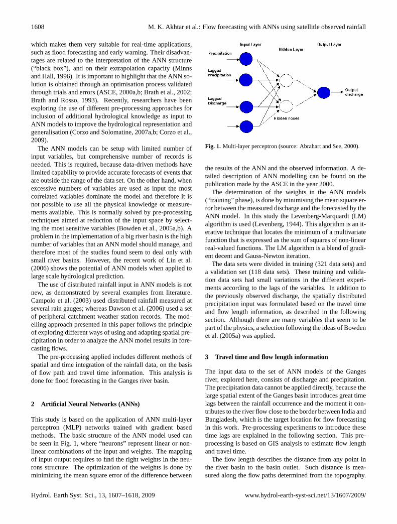
This study is based on the application of ANN multi-layerperceptron (MLP) networks trained with gradient basedmethods. The basic structure of the ANN model used canbe seen in Fig.1, where “neurons” represent linear or non-linear combinations of the input and weights. The mappingof input output requires to find the right weights in the neu-rons structure. The optimization of the weights is done byminimizing the mean square error of the difference between

Fig. 1. Multi-layer perceptron (source:Abrahart and See, 2000).

the results of the ANN and the observed information. A de-tailed description of ANN modelling can be found on thepublication made by the ASCE in the year 2000.

The determination of the weights in the ANN models(“training” phase), is done by minimising the mean square er-ror between the measured discharge and the forecasted by theANN model. In this study the Levenberg-Marquardt (LM)algorithm is used (Levenberg, 1944). This algorithm is an it-erative technique that locates the minimum of a multivariatefunction that is expressed as the sum of squares of non-linearreal-valued functions. The LM algorithm is a blend of gradi-ent decent and Gauss-Newton iteration.

The data sets were divided in training (321 data sets) anda validation set (118 data sets). These training and valida-tion data sets had small variations in the different experi-ments according to the lags of the variables. In addition tothe previously observed discharge, the spatially distributedprecipitation input was formulated based on the travel timeand flow length information, as described in the followingsection. Although there are many variables that seem to bepart of the physics, a selection following the ideas ofBowdenet al.(2005a) was applied.

3 Travel time and flow length information

The input data to the set of ANN models of the Gangesriver, explored here, consists of discharge and precipitation.The precipitation data cannot be applied directly, because thelarge spatial extent of the Ganges basin introduces great timelags between the rainfall occurrence and the moment it con-tributes to the river flow close to the border between India andBangladesh, which is the target location for flow forecastingin this work. Pre-processing experiments to introduce thesetime lags are explained in the following section. This pre-processing is based on GIS analysis to estimate flow lengthand travel time.

The flow length describes the distance from any point inthe river basin to the basin outlet. Such distance is mea-sured along the flow paths determined from the topography.

Hydrol. Earth Syst. Sci., 13, 1607–1618, 2009 www.hydrol-earth-syst-sci.net/13/1607/2009/

M. K. Akhtar et al.: Flow forecasting with ANNs using satellitle observed rainfall 1609

In GIS, the flow length of an arbitrary pixel is determined bysumming the incremental distances from centre-to-centre ofpixel along the flow path from the selected pixel to the outletpixel. The concept of flow length is an important issue to hy-drologists. When it rains, a drop of water landing somewherein the basin must first travel some distance before reachingthe outlet. Assuming constant flow velocities the pixel withthe greatest flow length to the outlet represents the hydrolog-ically most remote pixel. So, the time of concentration canbe obtained through flow length divided by the flow velocity.Therefore the time of concentration indicates how much timeis required for the entire basin to contribute to surface flowat the outlet, after a certain amount of rainfall. In watershedhydrology, there are various formulations (Izzard formula,Kerby formula, Kirpich formula, Bransby Williams equation,National Resources Conservation Service, Kinematic waveformula and etc.) to calculate time of concentration based onthe nature of flow as well as availability of information andscope of work (Wanielista, 1996).

The general assumption of calculating the travel time isthat a uniform velocity sustains throughout the basin, whichcan be interpreted as the Instantaneous Unit Hydrograph(IUH) function. IUH is defined as the flow response thatwould be observed at the basin outlet if a unit pulse of waterwere instantaneously placed uniformly over the entire riverbasin at a given instant. With the travel lengths known and asingle uniform velocity of flow observed throughout the wa-tershed, the travel time (tt i) to the outlet for any randomlychosen pixel,i, would be given by:

tt i = di/v (1)

Where,di is the distance fromith pixel to the watershedoutlet andv is the uniform flow velocity. This concept isexploited by using the Digital Elevation Models (DEMs) todiscern the flow organisation of the watershed and its uniquehydrologic signal (IUH) which is dependent on the watershedsize, shape, and connectivity.

The mentioned equation (Eq.1) neglects the velocity dif-ference between overland flow and river flow. An improve-ment to this approach is expected to come from introductionof different velocities for the overland and the river. Thisvelocity differences can be conceptually understood as com-ing from differences in the Mannings roughness (n) of theflow-surface encountered on the watershed versus the riverchannels. Velocity differences could be easily such that theriver flow velocities are 10 to 100 times larger then the over-land flow velocities (Moglen and Maidment, 2005). With thisapproach, a modified travel time can be applied:

tt i =dH,i

vH

+dC,i

vC

(2)

where,dH,i is the flow distance for pixeli, along the basin,dC,i is the flow distance for pixeli, along the river channel,vH is the overland velocity along the watershed,vC is the ve-locity along the river channel. If we consider the river basinas a system and its objective it is to drain water as quicklyas possible, then the presence of channel pixels with hightravel velocities represents efficiency within the system, asindicated by the small travel times associated with these pix-els.

An important consideration is the expected reduction inthe ANN processes to be represented due to the preprocess-ing transformation of the input precipitation.

4 Case Study: flood forecasting in Bangladesh

4.1 Study area and problem description

Bangladesh is a low-lying country located at the confluenceof three major rivers: the Ganges, the Brahmaputra and theMeghna (Fig. 2). About 92% of the catchment area of theserivers is located outside the country (Jakobsen and Bhuiyan,2005) and 80% of the annual rainfall occurs in the monsoonseason from June to September (Mirza, 2002). Thus hugecross-border monsoon flows, in addition to discharges fromlocal rainfall are drained through Bangladesh into the Bay ofBengal. In many occasions, the volume of generated runoffexceeds the capacity of the rivers, causing serious floodingin Bangladesh.

The river Ganges originates as the Bhagirathi from theGangotri Glacier in the Uttaranchal Himalaya and joins theAlaknanda near Deoprayang to form the Ganga. From there,the Ganges flows across the large plains of north India andempties in to the bay of Bengal after dividing up into manydistributaries (Fig.2). The source of the Ganges is at anelevation of 7010 m. The river has a bed slope of about1:10 000 in the stretch between the Allahabad and the Ba-naras. From the Banaras onward to the Calcutta the bed slopechanges from 1:12 000 to about 1:20 000. Along its greatlength, the Ganges passes through Bangladesh, which isalmost everywhere flat. The total length of the river is about2507 km. The Ganges has nine main sub-basins (Chambal,Betwa, Yamuna, Ramganga, Sone, Karnali, Gandak, Bag-mati and Kosi). The total basin area is 907×103 km2. Thefirst five tributaries originate in India and the last four tribu-taries join the Ganges from Nepal. Among these nine tribu-taries, the Yamuna is the most important one, which drainsabout one–third of the entire Ganges basin. The Kosi andKarnali drain about 12% and 9% of the basin, respectively(Mirza, 1997). In 1987, 1988, 1998 and 2004, several seri-ous floods occurred in Bangladesh, which are good examplesof the need for a forecasting and warning system as an essen-tial tool to reduce flood damage.

www.hydrol-earth-syst-sci.net/13/1607/2009/ Hydrol. Earth Syst. Sci., 13, 1607–1618, 2009


Fig. 2. Ganges-Brahmaputra-Meghna Basin.

In Bangladesh, there are about 52 forecasting stationswhere 24, 48, and 72-h forecasts are made every day (FFWC,2007). The lead-time of the model for the Northern part ofthe country is shorter. Improved model performance, in prin-ciple, can be achieved through regional cooperation amongthe countries that share the river basins in question, particu-larly for exchanging flood information and data sharing. Theactual model in Bangladesh consists of three modules: (a) arainfall-runoff modules (NAM), (b) a one-dimensional finitedifference hydrodynamic model (HD) based on St. Venantequations, (c) an updating module. The updating moduleanalyses measured and simulated water levels and dischargesup to the time of forecasting in order to eliminate amplitudeand phase errors which could influence the forecast results(Chowdhury, 2000). However the developed model can onlyforecast water level 3-day ahead for the Southern part of thecountry.

Due to regional limitation on the availability of data thecurrent physical based modelling of the region is more com-plex. The regional initiative of the World meteorologi-cal Organisation (WMO) and International Centre for Inte-grated Mountain Development (ICIMOD) is establishing aregional data exchange in the Hindukush Himalayan coun-ties (Bangladesh, India, Bhutan, Nepal, and Pakistan). How-ever, until now there is no significant improvement in datashearing, which hampers the expansion of the model bound-ary further upstream of the Brahmaputra and the Ganges.

Therefore, the major contribution of this case study is toexplore the possibility for provision of accurate flood fore-casts for the river Ganges, close to its entry point from Indiainto Bangladesh. If ANN models can provide sufficiently ac-curate forecasts several days ahead at this location, the lead-time for flood forecasting and warning within Bangladeshcan be extended, and the subsequent flood emergency mea-sures can be better planned and executed. The setup of theANN models is done by making use of freely available re-motely sensed (satellite) rainfall data and water level mea-surement records.

4.2 Tropical Rainfall Measurement Mission (TRMM)

Inputs to the ANN model are of critical importance. Satel-lite derived rainfall data of Tropical Rainfall MeasurementMission (TRMM,NASDA, 2001) is providing 3 hourly rain-fall, which is very promising. The reliability of the remotelysensed data is always facing challenges, but it is found fromvarious validation projects that precipitation radar of TRMMis producing error within acceptable range. However the ac-curacy of such data, when compared with rainfall observedfrom ground stations varies from place to place and it hasalready been tested over Bangladesh. The study proves thatthe correlation coefficient (R) is more than 0.773, which issensible to certain extent (Akhtar, 2006).

4.3 Data preparation

In this study, ANN is used to predict the river flow atHardinge Bridge (close to the entry point of the Ganges intoBangladesh, see Fig.2), utilising (i) the calculated dischargefrom water level gauge which is located at the same loca-tion (with known rating curve for conversion of water levelsinto discharges) and (ii) satellite based rainfall for the entirecatchment.

The documentation of satellite-derived rainfall is providedin Huffman et al. (2007) (ftp://meso-a.gsfc.nasa.gov/pub/trmmdocs/) and data from the Tropical Rainfall Measure-ment Mission are available in a regular 0.25 degree lat/longgrid (TRMM V6.3B42). The extracted data has resolution of0.25◦×0.25◦ (approximately: Lat. 27.7 km, Lon. 25.2 km),with a temporal resolution of three hour, which is accumu-lated to daily data for the period from 2001 to 2005. A dataprocessing tool has been developed to generate time seriesfor each pixel or areal average rainfall depending on the usersrequirement.

A DEM (digital elevation model) has been extracted fromthe website of Shuttle Radar Topography Mission (SRTM,http://www2.jpl.nasa.gov/srtm/) with a grid size of 1.0 km.The extracted DEM is then smoothened with ArcGIS andthen modified by FAP-19 (Flood Action Plan) information.Sinks (and peaks) are isolated grids with missing or abnor-mal values that often occur due to the resolution of the data orrounding of elevation to the nearest integer value. Sinks cangenerate discontinuity on the process of drainage networkderivation. The DEM has also been adjusted with knownriver lines and catchment boundaries.

Five years (from 2001 to 2005) of daily river flow datawas generated using rating equations based on the continuousobserved water level and validation discharge measurementsof Bangladesh Water Development Board (BWDB).

Both discharge and rainfall data from 2001 to 2003 wereselected for training, the data from 2004 to 2005 were se-lected for verification. Only high flow data were used to re-duce the influence of low flow condition as the study aims


ftp://meso-a.gsfc.nasa.gov/pub/trmmdocs/

ftp://meso-a.gsfc.nasa.gov/pub/trmmdocs/

http://www2.jpl.nasa.gov/srtm/


Fig. 3. Example of precipitation cluster-area analysis for 9th of July 2003.

to develop flood forecasting model. It is important to high-light that low flow are less dominated by the precipitation act-ing on previosu days and instead determined by the ground-water dynamics in the region. Therefore, the selection ofdata is reduced. The number of samples used for training to321 and 118 for verification. Statistical comparisons of themean, standard deviation and probability distribution of thedata sets has been performed. The results showed a goodagreement between the training and verification data sets.

In order to take into account the spatiotemporal distribu-tion of rainfall as an input to the ANN model, a GIS-basedanalysis of the satellite rainfall data has been carried outwhich resulted in areal clusters of rainfall data time-series,each with different lag time. The areal clusters have beendefined according to their calculated travel time to the outletof the catchment. In conventional approaches to such cluster-ing usually one average velocity is assumed for both overlandand channel flow. A new method has been applied here thatassumed different velocities for these two flow components(Sect. 3, Eq.2). The velocity along the river channel (vC)is assumed 1 m/s and the overland velocity along the water-shed is assumed 40 times smaller (vH =1/40 m/s), which iswithin the range indicated byMoglen and Maidment(2005),(10–100 times smaller).

Comparison of the areal clusters between the conventionaland the new method that has been applied here is presentedin Fig. 4aand b. The spatial distribution of equal travel timeareas is obviously coinciding with the drainage pattern byusing the new method.

Fig. 4a. Catchment delineation by travel time: velocity in channeland flood plain.

In the process of building the best ANN model, a 10-foldcross validation is performed. Figure5 shows the trainingand validation data sets, together with one of the 10 fold crossvalidation data sampled. It can be seen that the maximumand minimum values are in the same bounds. Although thedistribution seems shifted, its shape shows good agreementwith the training data set.

Subsequently to this analysis, a composite of the rainfalltime series was also generated by adding all the individ-ual areal rainfall time series, keeping in mind their lag time



Fig. 4b. Catchment delineation by travel time: conventional average velocity method.

Fig. 5. Probability distribution of training, cross validation and val-idation data sets.

(following the calculated travel times). It has been foundfrom correlation analysis that composite rainfall derivedfrom the new two-velocity travel time approach, demon-strates better correlation with the outlet discharge comparedto the conventional one.

Furthermore, in order to improve the performance of theANN model the usual practice is to consider previous dis-charges, as they contain more information than rainfall forlarger basins. Further correlation analysis has been carriedout to select the number of previous discharges, whichshowed that 1 day previous discharge should be included inthe input as it contains 99% information of the present dis-charge.

4.4 Modelling

4.4.1 ANN Setup

A number of scripts have been prepared to pre-process andanalyse the models using the ANN toolbox of Matlab. Theoptimal structure of the model was analysed by testing thetraining data set with different hidden nodes, ranging from 1to 10. Various combinations of input data are tested to com-pare and evaluate the sensitivity of the ANN. Fifteen differ-ent options were tested in an extensive analysis carried out byAkhtar (2006). Most of the result that excluded precipitationhad the disadvantage of performance reduction on the highflow situations. The results found are in accordance with thestudies done byToth(2008); Elshorbagy et al.(2009). In thispaper the options with most important results are discussedas follows:

[A] Only Discharge is used as input data (Only Q). Twodischarge time series, one of the present day and one of theday before, are used as input data for the ANN.

[B] Two discharges and 25 average areal rainfall withlagged time as input data (RF+Q). The area-average rainfalltime series are used with their respective lag time along withtwo discharge (present and 1 day before) time series.

[C] Two discharges, and lagged sum of the rainfall as inputdata (TRF+Q). All the 25 lagged area-average rainfall timeseries are added to form one, composite rainfall time series.Again two discharge (present and 1 day before) time seriesare used. The idea behind this reduction of the number ofrainfall time series is to test if ANN may be able to performbetter with fewer input data series.



Table 1. Root mean square error of the verification results for dif-ferent options.

Option Description 1 day 2 day 3 day 4 day 5 day

A Only Q 952 2108 3281 4432 5375B RF+Q 1117 2578 3730 6211 6244C TRF+Q 968 2223 3250 4322 5290D TRF+Q+Act.ET 968 2176 3390 4543 5427

[D] Two discharges, actual evapotranspiration and laggedsum of rainfall as input data (TRF+Q+Act.Evp). Actualevapotranspiration is used in this option as an input alongwith the other inputs of option [C], to take into account theevaporation losses. The actual evapotranspiration data weregenerated by a quasi-physically based model built with theSoil and Water Assessment Tool (SWAT).

4.4.2 Performance analysis

Training and verification has been performed for all differentANN model setups (option A to D). To measure the perfor-mance of the models, four criteria are selected, which areRoot Mean Square Error (RMSE), Normalised Root MeanSquare Error (NRMSE), Mean Average Error (MAE) andCorrelation coefficient (CoE,Nash and Sutcliffe, 1970). Adi-tionally the PERS index, which is a more conventional mea-sure for time series is included (Eq.6). Their values aresupplied in the following tables (Tables1 to 6). The errorscalculated numerically are supplemented by visual inspec-tion of the hydrographs (Fig.6) based on verification set.Root mean square error is calculated as:

RMSE=

√SSE

n(3)

SSE=

n∑t=1

(Qest,t − Qobs,t

)2 (4)

whereQobsandQestare the values of the observed and es-timated discharge, respectively. The total number of samplesis represented byn and the SSE is the abbreviation for thesum of square errors. Equation (3) is used to answer what isthe average magnitude of the forecast errors.

Sometimes it is important to compare two time series us-ing a reference of statistical properties of measurements.Therefore, here we use root relative squared error (Wittenand Frank, 2000), which compares the root square of themean of squared errors with the standard deviation of mea-surement. This means that we can see if the average errorsare outside of the standard deviation of measurements. Thismeasure is sometimes expressed as percentage, so a value of

Fig. 6a. Option A, only discharge Q.

Fig. 6b. Option B (distributed rainfall and discharge (RF+Q)) andC (composite rainfall and discharge (TRF+Q)).

Fig. 6c. Option C (composite rainfall and discharge (TRF+Q)) andD (discharge and actual evapotranspiration, (TRF+Q+Act. Evp)).



Table 2. Normalised root mean square error of the verification re-sults for different options.


A Only Q 8.937 19.76 30.7 41.4 50.1B RF+Q 10.49 24.17 34.91 58.01 58.2C TRF+Q 9.087 20.84 30.41 40.38 49.31D TRF+Q+Act.ET 9.09 20.4 31.73 42.43 50.59

Table 3. Mean abasolute error of the verification results for differ-ent options.


Only Q 681.4 1602 2592 3398 4288B RF+Q 847.7 1965 2948 4939 4891C TRF+Q 688.9 1676 2535 3421 4292D TRF+Q+Act.ET 687.9 1641 2564 3507 4443

100% means that the RMSE is in the bound of the standarddeviation. If the errors are much higher than these boundvalues the root relative squared error will be above 100%. Inthis sense the root relative error is a Normalized Root MeanSquare, term used in this thesis (NRMSE, Eq.5).

NRMSE=

√SSEn

σobs(5)

Where the value ofσ is the standard deviation of the mea-sured or observed discharges.

The persistence index (PERS) focuses on the relationshipof the model performance and the performance of the naıve(“no-change”) model which assumes that the forecast at eachtime step is equal to the current value (Kitanidis and Bras,1980):

PERS= 1 −SSE

SSEn

(6)

SSEn =

n∑t=1

(Qobs,t+L − Qobs,t

)2 (7)

SSEn is a scaling factor based on the performance of thenaıve model;Qest,t is the DDM forecast or a process-basedmodel simulation of the next time step,Qobs,t is the observeddischarge at timet wheret=1, 2, . . . , n; L is the lead time(L=1 for one day ahead forecast); andn is the number ofsteps for which the model error is to be calculated.

PERS is a unit that is relative to the naıve model. Itcan range between 1 and minus infinite (i.e. it is degradingthe provided information), values above 0 indicate that theconsidered model is better than the naıve model (where the

Fig. 7a. Comparison between target and predicted values togetherwith errors (NRMSE) for Option C in training stage.

(a) Comparison between target and predicted values together with errors

(NRMSE) for Option C in training stage

(b) Comparison between target and predicted values together with errors

(NRMSE) for Option C in cross-validation stage

(c) Comparison between target and predicted values together with errors

(NRMSE) for Option C in verification stage

Fig. 717

Fig. 7b. Comparison between target and predicted values togetherwith errors (NRMSE) for Option C in cross-validation stage.

(a) Comparison between target and predicted values together with errors

(NRMSE) for Option C in training stage

(b) Comparison between target and predicted values together with errors

(NRMSE) for Option C in cross-validation stage

(c) Comparison between target and predicted values together with errors

(NRMSE) for Option C in verification stage

Fig. 717

Fig. 7c. Comparison between target and predicted values togetherwith errors (NRMSE) for Option C in verification stage.



Fig. 8: Comparison of correlation coefficients for Options A (only Q) and Option C (TRF+Q) for

extended forecast horizon up to 10 days.

Comparison of Discharge Hydrograph (E)

09/01/2001 28/07/2001 13/02/2002 01/09/2002 20/03/2003 06/10/2003 23/04/2004 09/11/2004 28/05/2005

Time

0

50000

100000

150000

200000

250000

300000

350000

400000

To

tal ra

infa

ll(m

3/s

)

rated discharge

Simulation result

Total Rainfall

Fig. 9: Hydrograph comparison between SWAT model simulation results and the rated discharge

18

Fig. 8. Comparison of correlation coefficients for Options A (onlyQ) and Option C (TRF+Q) for extended forecast horizon up to 10days.

closer to 1 the better), and negative values show less perfor-mance than the naıve model. Lauzon et al.(2006) suggestusing PERS in cases when the discharge forecast is made onthe basis of previous values.

For each option (A–D), five different simulations are per-formed to check the performance of the model for a 1-day,2-day, 3-day, 4-day and 5-day forecast horizon. The resultsindicate that the model performance is showing decreasingtrend with the increase of lead-time. However, from the sim-ulated hydrographs and performance tables, it is establishedthat forecasting performance is acceptable up to 3-days. Be-yond this period, results are getting worse. To keep the dis-cussion within limits and also to review the results metic-ulously, 3-day forecast (verification) results are discussedhere. The results of the 3-day forecasts are shown in Fig. 6.

Option [A], with only Q time series as input, does notshow large differences from the options where rainfall timeseries are included (Fig.6a). Option [C] exhibits some im-provement in the forecasting performances compared to Op-tion [B], which can also be seen from the performance cri-teria tables (Tables1 to 6). This indicates that large numberof input parameters is not suitable to develop an ANN for abasin area like the Ganges. After inclusion of the actual evap-otranspiration as a separate time series in Option [D], Fig.6cand the performance analysis criteria (Table1 to 6) indicatedeterioration of model result. This is most likely due to veryhigh uncertainty of the SWAT model results which were usedfor generating the time series of actual evapotranspiration.Assessment of the values of the performance analysis tablesindicates that option [C] is most suitable for flood forecastingof Ganges basin with a 3-day forecast horizon.

Figure7 has been introduced to visualise the performanceof the model (option C) by comparison plots of training,cross-validation and verification as well as errors analysisin terms of NRMSE. It shows that there is an excellentagreement between the observed and simulated data for thetraining phase but the performance deteriorates in the cross-

Table 4. Correlation coefficient of the verification results for differ-ent options.


A Only Q 0.996 0.98 0.952 0.911 0.866B RF+Q 0.995 0.971 0.938 0.821 0.817C TRF+Q 0.996 0.978 0.953 0.915 0.87D TRF+Q+Act.ET 0.996 0.979 0.948 0.906 0.863

Table 5. Mean of the forecast predictions.

Option Description 1 day 2 days 3 days 4 days 5 days

A Only Q 2.6544 2.6635 2.6508 2.6495 2.654B RF+Q 2.6536 2.6598 2.6941 2.723 2.6018C TRF+Q 2.6521 2.6474 2.6522 2.6517 2.6512D TRF+Q+Act. ET 2.652 2.6523 2.5773 2.6202 2.6715

validation stage. However, model performance in the veri-fication stage is satisfactory, as several peaks show good re-semblance with observation.

Moreover, accurate timing is also important and is a crit-ical factor in operational management and decision-makingactivities related to high magnitude flood events. Timing er-rors (phase lag) of the model results have, however, beenidentified from all the options. This is a common problemin neural network rainfall-runoff models and causes are stillunder investigation by neuro-hydrologists. One approach tothis problem (as suggested byAbrahart et al., 2007) is to usea time-error correction procedure as an integrated part of theneural network optimisation process. However, at the timeof this writing the full description of this procedure was notavailable for testing.

Note that Fig.7ais not completely continuous in time andin sample 116, 28 October 2001, there is a gap of low flows,so sample 117 corresponds to 9 July 2002. Figures7b and care continous in time for all the time series plot. Their timeframe is between 5 July 2003 till 5 October 2003 and 1 July2004 till 26 October 2004, respectively.

4.4.3 Expanded forecast horizons

The similar performance of option [A] to options [B,C,D]confirms that for short- to medium-term forecasts and forlarge rivers, ANN can provide good forecasts based only oncurrent and previous discharge measurements. For long-termforecasts it is expected that this predictability on the basisof real-time discharge measurements decreases. In that caserainfall information and rainfall-runoff modelling would be-come more important. To investigate whether this applies tothe Ganges case study, forecasting horizon is increased from5 days to 10 days for option [A] (only Q), and option [C](TRF + Q). The correlation performance of the two ANNsis presented in Fig.8. It shows that for forecast horizonsfrom 7–10 days the inclusion of the rainfall as an input to



Fig. 9. Hydrograph comparison between SWAT model simulation results and the rated discharge.

Table 6. PERS index of the verification results for different options.

Option Description 1 day 2 days 3 days 4 days 5 days

A Only Q 0.647 −0.7107 −3.3473 −7.4138 −11.5369B RF+Q 0.5783 −1.2459 −3.6998 −2.0217 −12.1628C TRF+Q 0.6836 −0.6696 −2.5676 −5.3076 −8.4465D TRF+Q+Act. ET 0.6832 −0.6 −3.23 −5.615 −8.9429

the ANN (option [C]), improves the forecasting performance.Note that with the increase of forecasting horizon, the perfor-mance of the model is getting worse and the performance ofthe forecast beyond three days is not acceptable, whateverimprovement can be seen by including the rainfall. Howeverthis exercise proves that composite rainfall (which is satellitedriven) along with previous discharge can help to build betterANN, for longer forecasting lead times.

Figure9 shows the rated and simulated discharge togetherwith total rainfall over the catchment. This simulated dis-charge is the best performed simulation output of our SWATmodel setup. The results presented in this paper were com-pared to the Soil Water Assessment Tool (SWAT) model ofthe basin. Although a number of complex optimization algo-rithms were tested, the SWAT model results did not achievethe performance of the ANN model results presented here(van Griensven et al., 2007). The errors for the SWAT modelresults were a RMSE of 11600, a MAE of 8930 and a Cor-relation coefficient of 0.359. This is most likely due to thelarge spatial extension of the basin and lack of information oncatchment parameters data, as required for the SWAT model.

5 Conclusions

An ANN flow forecasting model that makes use of spatialprecipitation obtained from pre-processing based on hydro-logical concepts of travel time and flow length has beendeveloped for the Ganges river basin. This was done bycombining ground station flow measurements with satellitederived rainfall and DEMs, and hydrological GIS analyses.A new method for estimation of travel time has also beenapplied and tested with artificial neural networks.

From the analysis of various options for input data, it wasrevealed that the forecasted discharge is highly influencedby the previous discharge input data, because of their strongcorrelation. This was expected, particularly because of theexceptionally large spatial scale of the river. For this rea-son, different combinations of rainfall input did not influencethe model much for the short forecast horizons, For forecasthorizons of 7 to 10 days inclusion of rainfall information inaddition to discharge data, improves the ANN model perfor-mance.

Accurate timing is a critical factor in operational manage-ment and decision-making activities related to high magni-tude flood events. Timing errors (phase lag), however, havebeen identified, which is a common problem in ANN rainfall-runoff models. Inclusion of a time-error correction proce-dure as an integral part of the ANN optimisation process canimprove the model performance.

The finally selected ANN model shows some disagree-ment with the observed values, especially during the peakdischarge. The causes may be hidden within the unknownprocesses of the catchment, unverified rainfall data and rateddischarge, etc. For further improvement of the model, itis essential to investigate the target value (rated discharge),



where discharge is generated from a conventional ratingcurve.

The method that has been used to calculate travel-time anddelineate the clustered areas, from which water can reachthe outlet of the basin within a certain range of time, can befurther improved. In this study only two different velocitieswere assumed, one for channels and the other for land surfaceflow, but in reality the velocity is not the same in all rivers,even velocity differs from reach to reach of a river. Surface-runoff velocity is also considered constant for all over thebasin, irrespective of land use and land slope, which is con-trary of the physical conditions. More detailed velocity esti-mates by considering the land use characteristics can help toimprove the model performance.

From the overall analysis it is found that one-day previousdischarge along with composite rainfall (derived from GIS-based travel time calculation) gives the best result comparedto other options. This shows that remote sensing techniquesand data driven modelling can be combined successfully toprepare a spatially distributed ANN for flow forecasting oflarge-scale river basins like the Ganges.

The study presented is a particular case and the findingshere can be tested and extended in further research. Thismethodology will be explored and benchmarked togetherwith other methodologies reported in literature, specially onsmaller catchments in order to see the effect of distributedrainfall input more clearly.

Acknowledgements.This study was possible due to the financialsupport provided by the Delft Cluster project in the Netherlands.Many thanks to Editor N. Verhoest for his careful editing whichgreatly improves the manuscript.

Edited by: N. Verhoest

References

Abrahart, R. J. and See, L.: Comparing neural network and autore-gressive moving average techniques for the provision of conti-nous river flow forecasts in two contrasting catchments, Hydrol.Process., 14, 2157–2172, 2000.

Abrahart, R. J., Heppenstall, A. J., and See, L. M.: Timing error cor-rection procedure applied to neural network rainfall-runoff mod-elling, Hydrolog. Sci. J., 52, 414–431, 2007.

Akhtar, M. K.: Flood Forecasting for Bangladesh with satel-lite Data, Msc Thesis, UNESCO-IHE, Delft, the Netherlands,134 pp., 2006.

ASCE: Task Committee on Application of Artificial Neural Net-works in Hydrology, Artificial Neural Networks in Hydrology,II:Hydrologic Application, J. Hydrol. Eng., 5, 124–136, 2000a.

ASCE: Task Committee on Application of Artificial Neural Net-works in Hydrology, Artificial Neural Networks in Hydrology. I:Preliminary Concepts, J. Hydrol. Eng., 5, 115–123, 2000b.

Bowden, G. J., Dandy, G. C., and Maier, H. R.: Input determinationfor neural network models in water resources applications. Part1-background and methodology, J. Hydrol., 301, 75–92, 2005a.

Bowden, G. J., Dandy, G. C., and Maier, H. R.: Input determinationfor neural network models in water resources applications. Part2. Case study: forecasting salinity in a river, J. Hydrol., 301, 93–107, 2005b.

Brath, A. and Rosso, R.: Adaptive calibration of a conceptual modelfor flash flood forecasting, Water Resour. Res., 29, 2561–2572,1993.

Brath, A., Montanari, A., and Toth, E.: Neural networks and non-parametric methods for improving real-time flood forecastingthrough conceptual hydrological models, Hydrol. Earth Syst.Sci., 6, 627–639, 2002,http://www.hydrol-earth-syst-sci.net/6/627/2002/.

Campolo, M., Soldati, A., and Andreussi, P.: Artificial neural net-work approach to flood forecasting in the River Arno/Une ap-prochea base de reseau de neurones artificiels pour la previsiondes crues du fleuve Arno, Hydrolog. Sci. J., 48, 381–398, 2003.

Chowdhury, M.: An assessment of flood forecasting in Bangladesh:the experience of the 1998 flood, Nat. Hazards, 22, 139–163,2000.

Corzo, G. and Solomatine, D.: Knowledge-based modularizationand global optimization of artificial neural network models inhydrological forecasting, Neural Networks, 20, 528–536, 2007a.

Corzo, G., Solomatine, D., Hidayat, de Wit, M., Werner, M., Uh-lenbrook, S., and Price, R.: Combining semi-distributed process-based and data-driven models in flow simulation: a case study ofthe Meuse river basin, Hydrol. Earth Syst. Sci. Discuss., 6, 729–766, 2009,http://www.hydrol-earth-syst-sci-discuss.net/6/729/2009/.

Corzo, G. A. and Solomatine, D. P.: Baseflow separation techniquesfor modular artificial neural networks modelling in flow forecast-ing, Hydrolog. Sci. J., 52, 491–507, 2007b.

Dawson, C., See, L., Abrahart, R., and Heppenstall, A.: Symbioticadaptive neuro-evolution applied to rainfall–runoff modelling innorthern England, Neural Networks, 19, 236–247, 2006.

Elshorbagy, A., Corzo, G., Srinivasulu, S., and Solomatine, D.:Experimental investigation of the predictive capabilities of softcomputing techniques in hydrology., Technical Rep., 49 pp.,2009.

FFWC: Flood Forecasting and Warning Centre; Annual Flood Re-port 2007, Technical Rep., Dhaka, Bangladesh, 4, 86 pp., 2007.

Huffman, G., Adler, R., Curtis, S., Bolvin, D., and Nelkin, E.:Global rainfall analyses at monthly and 3-hr time scales, Mea-suring Precipitation from Space: EURAINSAT and the Future,Springer, Dordrecht, The Netherlands, 28, 291–305, 2007.

Jakobsen, F., Hoque, A. K. M. Z. , Paudyal, G. N., and Bhuiyan,S.: Evaluation of the Short-Term Processes Forcing the Mon-soon River Floods in Bangladesh, Hydrolog. Sci. J., 30, 389–399,2005.

Kitanidis, P. K. and Bras, R. L.: Real-Time Forecasting With a Con-ceptual Hydrologic Model: Analysis of Uncertainty, Water Re-sour. Res., 16, 1025–1033, 1980.

Lauzon, N., Anctil, F., and Baxter, C. W.: Clustering of het-erogeneous precipitation fields for the assessment and possibleimprovement of lumped neural network models for streamflowforecasts, Hydrol. Earth Syst. Sci., 10, 485–494, 2006,http://www.hydrol-earth-syst-sci.net/10/485/2006/.

Levenberg, K.: A method for the solution of certain problems inleast squares, Quart. Appl. Math, 2, 164–168, 1944.

Lin, J., Cheng, C., and Chau, K.: Using support vector machines for


http://www.hydrol-earth-syst-sci.net/6/627/2002/

http://www.hydrol-earth-syst-sci-discuss.net/6/729/2009/

http://www.hydrol-earth-syst-sci.net/10/485/2006/


long-term discharge prediction, Hydrolog. Sci. J., 51, 599–612,2006.

Minns, A. W. and Hall, M.: Artificial Neural Networks as rainfall-runoff models, Hydrolog. Sci. J., 41, 399–417, 1996.

Mirza, M.: The runoff sensitivity of the Ganges river basin to cli-mate change and its implications, J. Environ. Hydrol., 5, 1–13,1997.

Mirza, M.: Global warming and changes in the probability of oc-currence of floods in Bangladesh and implications, Global Envi-ronmental Change, 12, 127–138, 2002.

Moglen, G. E. and Maidment, D. R.: Digital Elevation Model Anal-ysis and Geographic Information Systems, Encyclopedia of Hy-drological Sciences, Part 2., Hydroinformatics, Vol. 1, John Wi-ley & Sons, Ltd., Chichester, England, UK, 239–255, 2005.

NASDA: TRMM data users Handbook, Technical Rep., 226 pp.,2001.

Nash, J. E. and Sutcliffe, J. V.: River flow forecasting through con-ceptual models Part 1- A Discussion Principles, J. Hydrol., 10,282–290, 1970.

Toth, E.: Data-Driven Streamflow Simulation: The Influence of Ex-ogenous Variables and Temporal Resolution, in: Practical Hy-droinformatics: Computational Intelligence and TechnologicalDevelopments in Water Applications, edited by: Abrahart, R.J., Linda, M. S., and Dimitri, P., Solomatine, Berlin Heidelberg,Germany, 2008.

van Griensven, A., Akhtar, M. K., A., Haguma, D., Sintayehu, R.,Schuol, J., Abbaspour, K., van Andel, S., and Price, R.: CATCH-MENT Modeling using Internet-Based Global Data, 4th SWATconference UNESCO-IHE Delft, The Netherlands, 2007.

Wanielista, M. P., Kersten, E., and Robert, R.: Hydrology: WaterQuantity and Quality Control, John Wiley and Sons, Ltd., NewYork, USA, 567 pp., 1996.

Witten, I. H. and Frank, E.: Data Mining: Practical Machine Learn-ing Tools and Techniques with Java Implementations, MorganKaufmann, 525 pp., 2000.


River ﬂow forecasting with artiﬁcial neural networks using ... there are various formulations...

Documents

Transcript of River ﬂow forecasting with artiﬁcial neural networks using ... there are various formulations...