Risk Parity approach to Asset Allocation
99
COPENHAGEN BUSINESS SCHOOL Master Thesis MSc.ASC RISK PARITY APPROACH TO ASSET ALLOCATION Author: Jacob Buhl Jensen Supervisor: Daniel W. Probst A thesis submitted in fulfilment of the requirements for the degree of MSs ASC in the Department of Operations Management Copenhagen Business School 17 September, 2013 154.594 characters / 80 pages
Transcript of Risk Parity approach to Asset Allocation

COPENHAGEN BUSINESS SCHOOL
Master ThesisMSc.ASC
RISK PARITY APPROACH TO ASSETALLOCATION
Author:
Jacob Buhl Jensen
Supervisor:
Daniel W. Probst
A thesis submitted in fulfilment of the requirements
for the degree of MSs ASC
in the
Department of Operations Management
Copenhagen Business School
17 September, 2013
154.594 characters / 80 pages

Risk Parity approach to Asset Allocation
Jacob Buhl Jensen†
17 September, 2013
Keywords: Asset Allocation, Risk Parity, Risk-Based Portfolios, Portfolio Optimization
ABSTRACT: Since the financial crisis, portfolios based on risk diversification are of greatinterest to both academic researchers and market practitioners. They have been employed byseveral asset mangement firms and their performance appears promising. Since they do notrely on estimates of expected returns, they are assumed to be more robust. Of the multitudeof alternative asset allocation portfolios that are being proposed, a collection of approachesbroadly referred to under the heading of Risk Parity seems to be gaining traction.
This thesis presents a review of asset allocation strategies and develops and backtests theseportfolio strategies in a consistent framework. Reviewed are four risk-based portfolios, GlobalMinimum-Variance, Inverse Volatility, Most Diversification Portfolio and Risk Parity. In ad-dition, the traditional 60/40 portfolio is applied, reflecting a portfolio strategy applied by along-term investor. This thesis uses an evaluation methodology that consider risk adjustedreturns, maximum drawdowns, diversification ratio, turnover and risk contribution. Based onthree emperical backtests some very attractive aspects are to be found in the Risk Parity ap-proach to asset allocation. First, it purports to reduce the dependence on statistical parameters,such as returns, that are difficult to estimate. Second, for a given level of risk, when measured asportfolio volatility, it is much more diversified than an any other portfolio strategy. Third, whenleverage is applied the risk adjusted performance is superior. However, turnover and associatedtransaction costs can be a substantial drag on returns. Further, the drawdowns in a Risk Paritystrategy can be a significant factor when determining ones asset allocation strategy.
When backtested on market data, all risk-based portfolios are shown to be effective in improvingportfolio performance over the traditional 60/40 portfolio. Yet, the performance within eachrisk-based portfolio is mixed. The Inverse Volatility portfolio requires no optimization makingit less complex than any of the other portfolio strategies. Nevertheless, the portfolio strategydisplays good risk adjusted returns relative to a low turnover. The Global Minimum-Varianceportfolio exhibits great risk adjusted returns at the expense of high portfolio turnover. TheMost Diversification Portfolio entails the highest ex-ante diversification but delievers lower riskadjusted returns than the Global-Minimum Variance and at a higher turnover.
Contents
1 Introduction 1
1.1 Background . . . . . . . . . . . . . . . . . . . . . . . . . . . . . . . . . . . . . . . 2
1.2 Motivation . . . . . . . . . . . . . . . . . . . . . . . . . . . . . . . . . . . . . . . 3
1.3 Research question . . . . . . . . . . . . . . . . . . . . . . . . . . . . . . . . . . . . 5
1.4 Outline . . . . . . . . . . . . . . . . . . . . . . . . . . . . . . . . . . . . . . . . . 6
1.5 Limitations . . . . . . . . . . . . . . . . . . . . . . . . . . . . . . . . . . . . . . . 6
I The Quest for Returns in New Economic Regimes 7
2 The death of Markowitz optimization? 8
2.1 From Asset Allocation by the book to practical Asset Allocation . . . . . . . . . 10
2.2 Asset Allocation by the 21st century . . . . . . . . . . . . . . . . . . . . . . . . . 11
2.3 Improving the quality of input estimates . . . . . . . . . . . . . . . . . . . . . . . 13
2.4 Reducing dependency on expected return . . . . . . . . . . . . . . . . . . . . . . 14
2.5 Case study: Risk Parity in ATP . . . . . . . . . . . . . . . . . . . . . . . . . . . 15
3 A Changed World 18
3.1 Central Banks and Their Bazookas . . . . . . . . . . . . . . . . . . . . . . . . . . 19
3.2 Lessons Applied by QE . . . . . . . . . . . . . . . . . . . . . . . . . . . . . . . . 22
3.3 Asset Allocation in Low Yield Environment . . . . . . . . . . . . . . . . . . . . . 23
II On the Properties of Risk-Based Asset Allocation with Empirical Re-sults 26
4 Theoretical Framework 27
4.1 Portfolio terminology . . . . . . . . . . . . . . . . . . . . . . . . . . . . . . . . . . 28
4.1.1 Returns . . . . . . . . . . . . . . . . . . . . . . . . . . . . . . . . . . . . . 28
4.1.2 Sharpe Ratio . . . . . . . . . . . . . . . . . . . . . . . . . . . . . . . . . . 30
4.1.3 Risk factors . . . . . . . . . . . . . . . . . . . . . . . . . . . . . . . . . . . 31
4.2 Fundamentals of Risk Parity portfolio . . . . . . . . . . . . . . . . . . . . . . . . 32
ii

Contents iii
4.3 Benchmark strategies . . . . . . . . . . . . . . . . . . . . . . . . . . . . . . . . . . 35
4.3.1 Traditional 60/40 portfolio . . . . . . . . . . . . . . . . . . . . . . . . . . 36
4.3.2 Inverse Volatility portfolio . . . . . . . . . . . . . . . . . . . . . . . . . . . 36
4.3.3 Global Minimum-Variance portfolio . . . . . . . . . . . . . . . . . . . . . 37
4.3.4 Maximum Diversification portfolio . . . . . . . . . . . . . . . . . . . . . . 38
5 Emperical Results 40
5.1 Portfolio construction and backtesting setup . . . . . . . . . . . . . . . . . . . . . 40
5.2 Methodology for evaluating portfolio performance . . . . . . . . . . . . . . . . . . 42
5.2.1 Maximum Drawdown . . . . . . . . . . . . . . . . . . . . . . . . . . . . . 43
5.2.2 Diversification ratio . . . . . . . . . . . . . . . . . . . . . . . . . . . . . . 43
5.2.3 Turnover . . . . . . . . . . . . . . . . . . . . . . . . . . . . . . . . . . . . 43
5.3 Global Diversified Portfolios . . . . . . . . . . . . . . . . . . . . . . . . . . . . . . 44
5.4 Global Portfolios . . . . . . . . . . . . . . . . . . . . . . . . . . . . . . . . . . . . 53
5.5 World Equity Sectors Portfolios . . . . . . . . . . . . . . . . . . . . . . . . . . . . 61
III Robustness of Risk Parity 67
6 The impact of biases in Asset Allocation 68
6.1 Pitfalls of backtesting . . . . . . . . . . . . . . . . . . . . . . . . . . . . . . . . . 69
6.1.1 Rebalancing . . . . . . . . . . . . . . . . . . . . . . . . . . . . . . . . . . . 70
6.1.2 Parameter estimation period . . . . . . . . . . . . . . . . . . . . . . . . . 70
6.1.3 Cost of borrowing . . . . . . . . . . . . . . . . . . . . . . . . . . . . . . . 71
6.2 Pitfalls of Risk Parity . . . . . . . . . . . . . . . . . . . . . . . . . . . . . . . . . 71
6.2.1 Rising yields . . . . . . . . . . . . . . . . . . . . . . . . . . . . . . . . . . 72
6.2.2 Leverage . . . . . . . . . . . . . . . . . . . . . . . . . . . . . . . . . . . . . 73
6.2.3 Return distribution . . . . . . . . . . . . . . . . . . . . . . . . . . . . . . . 74
IV Discussion 75
7 Conclusion 76
Bibliography 78
A Derivation of the CAPM Equation 82
B Derivation of MRC and TRC 84
C Figures of robustness check 86
D Matlab code 90

Chapter 1
Introduction
To anyone who has researched the risk allocation of the classical 60/40 portfolio and its return
implications, the large drawdowns to many institutional portfolios during the financial crisis
should not be surprising. The fact is that a 60/40 portfolio does not offer true diversification
due to 80-90% of its risk profile is contributed by equity while the remaining fixed income
instruments contribute with only 10-20% to the overall risk. By definition, equities are typically
considered to be more risky than bonds and, all else being equal, investors who follow such
allocation end up with a highly concentrated risk allocation.
Traditional strategic asset allocation theory is deeply rooted in the mean-variance portfolio op-
timization framework developed by Markowitz (1952)[32] for constructing portfolios. However,
the mean-variance optimization methodology is difficult to implement due to the challenges
associated with estimating the expected return and covariances for asset classes with accuracy.
Subjective estimates on forward returns and risks can often be influenced by individual biases
of the investor, such as overestimating expected returns due to the recent strong momentum of
an asset class or the other way around, underestimate risk because of personal interpretation
on the distribution of returns which may results in ignoring fat tails when markets frozen. As
such, parameter estimation based on historical data can be exposed to noise, especially if risk
premia and correlations are time varying1.
1 See Merton (1980)[34] for a discussion on the impact of time varying volatility on the estimate for expectedreturns. Further, Cochrane (2005)[11] discuss the time varying equity premium and models for forecasting equityreturns and Campbell (1995)[4] reflects on the bond premium
1

Chapter 1. Introduction 2
1.1 Background
The natural reaction to any crises, once the imminent danger has subsides, is to look back,
evaluate what went wrong and develop strategies to avoid or mitigate the impact of future
crises with similar characteristics. The recent financial crisis is no expection. As markets has
begun to recover, practitioners and academics alike have disgorged a seemingly endless litany
of ’next generation solutions’ to everything that went wrong with the financial sector. One of
the more common refrains has been an attack on the mean-variance framework as well as the
traditional 60/40 split between equities and bond which is central to the asset allocation process
employed by many institutional as well as private investors.
On one hand, these new models and theories which seem to gain significant traction due to a
better protection against substantial losses next time equity and credit market tightness, should
be viewed with a great deal of scepticism as they are bound to incorporate a healthy dose of
data mining and fitting biases. On the other hand, so far, the twenty-first century has not been
in line with good performance for most institutional investors. US equities underperformed
not only expectations, but fixed income as well, calling for the Risk Parity has flourished, not
only because it (usually) leveraged fixed income exposure has experiened high returns, but also
because it advances a novel investment principle; The key to asset allocation is to allocate equal
shares of portfolio risk to each asset class.
Table 1.1: Key statistics of MSCI World Index and J.P. Morgan Aggregate BondIndex, 1990-Q12013
MSCI World Index J.P. Morgan Aggregate Bond Index
Mean ann. (%) 5.19 7.12Standard deviation ann. (%) 18.05 6.52Skewness ann. -0.65 0.12Kurtosis ann. 1.29 0.46
Rolling Sharpe Ratio 0.20 0.32
Note: The Sharpe ratio is 6 month rolling. Source: Bloomberg
As shown in table 1.1 MSCI World Index has underperformed J.P. Morgan Aggregate Bond
Index by 1.93% a year since 1990, with volatility of the bond index being 1/3 of the volatility of
the equity index. Similarly, table 1.1 shows rolling 6 month Sharpe Ratios which clearly indicates
that J.P. Morgan Aggregate Bond Index has outperformed MSCI World Index during the last
two decades. One could argue that going forward it is difficult for the bond index to repeat the
Chapter 1. Introduction 3
performance of the last 22 years. Therefore, any model that recommends a significant allocation
to fixed income should be carefully analyzed and its assumptions should be questioned.
Moreover, the important question for investors is whether Risk Parity will work as well in the
future. This is more a matter of the investment principles it involves than whether bonds will
continue to outperform equities. The aim of this thesis in the following chapters is to under-
stand and evaluate these investment princicples as well as making an comparison with relevant
benchmarks strategies. Ultimately, based on the emperical backtests, the thesis incorporate
their positive contribution as well as drawbacks into an improved approach to strategic asset
allocation.
1.2 Motivation
After a decade of extremely high macroeconomic uncertainties and increased volatility within
the equity markets, investors have started to rethink their traditional asset allocation models
that have often fallen short of expected risk reward. For that reason, new risk-based portfolio
construction techniques, like Risk Parity, have become popular among researchers and investors.
The crisis of the last decade have highlighted several inconvenient truths about the evolution
of asset management and asset allocation. First, investing in pure asset classes and passive,
market-capitalization benchmarks has not met investors needs and has resulted in inadequate
and highly volatile returns. Second, institutions have learned the hard way that risk-neutral
portfolios are not actually risk neutral. If a portfolio is not adequately diversified, a major
market or liquidity event can wipe out the accumulated alpha. Third, increasing the number
of asset classes in a portolio does not always increase effective diversification beacuse many of
the so-called new asset classes have the same types of risks and exposures as traditional asset
classes.
Based on the lessons learned from these inconvenient truths, asset allocation researchers and
practioners are building new approaches to address the range of challenges that lie ahead.
The latter challenge represents the highly increased cross-market correlations. Fourty years
ago, as portfolio managers began to add international equity and fixed income to a portfolio
of domestic equity and fixed income, diversification improved because cross-market correlations
were low. But progressive globalization of markets combined with global quantitative easing and
financial engineering has dramatically reduced the diversification effect of cross-asset allocation.

Chapter 1. Introduction 4
Together with low correlations across asset classes it is desirable to have reasonable long term
risk adjusted return expectations. However, as the world enters new economic regimes, asset
managers find it difficult to meet long term return targets with reasonable associated risk. As
stated in table 1.1 fixed income has outperformed equities the last two decades. Moreover, the
Sharpe ratio has diminished significantly during this sample period. The average risk adjusted
return of the MSCI World Index has dropped from 0.39 over the last two decades to just 0.04 over
the last five years (2007-2012). Similarly, the Sharpe ratio of S&P 500 from 1992 to 2012 was
0.43, but during the last five years, it has been only 0.08, and the MSCI Emerging Markets Index
average risk adjusted return has fallen from 0.53 to 0.07 (see Straatman (2013)[45]). Further,
the drawdowns for equities have been increasing over the last decade as well as illustrated in
figure 1.1. At the expense of the poor performance of equities, the great performer in the global
financial markets has been fixed income instruments, measured not only by average return but
also average risk adjusted return.
Figure 1.1: Implied volatility of MSCI World Index (Upper left), J.P. Morgan Aggre-gate Bond Index (upper right), and the five largest relative drawdowns in equity bear
markets, 2003-Q12013
Source: Bloomberg
A relevant question to ask is whether Risk Parity make sense in the current environment, when
interest rates are likely to rise in the medium to long term perspective? Recent evidence clarify
that Risk Parity has been a good solution in the past. Being able to leverage up low volatile asset
classes, such as fixed income, to reproduce equity returns without having the same volatility has

Chapter 1. Introduction 5
worked well. Over the next couple of years, opportunities to leverage a low volatile asset class to
get equity returns might seem unlikely2. In constrast, by producing an acceptable Sharpe ratio
and managing drawdown risk properly, high volatile asset classes can strengthen the overall
portfolio performance because managers will not be relying entirely on fixed income to provide
leverage.
1.3 Research question
One of the well-known rules in asset allocation is that an investor should not put all eggs in
one basket. Some investors do not seem concerned by risk contribution and are thinking that a
traditional 60/40 portfolio offers a real diversified portfolio.
This thesis will adress the problem facing investors in seeking to form an truly diversified optimal
asset allocation strategy. As such, the thesis follows the footsteps of Maillard et. al (2010)[14]
who was the first to solve such problems in detail and whom advocate the Risk Parity paradigm
in general. More specifically, the aim of the thesis is twofold. First, the Risk Parity paradigm in
portfolio construction and its unique construction method is examined based on the simple idea
that the allocation of risk must be done with the same level of risk for all assets in the portfolio.
In order to dwell on the Risk Parity approach to asset allocation, four well-known portfolios are
applied as benchmark strategies. Moreover, the portfolios are the traditional 60/40 portfolio
which represents the widely applied portfolio among institutional and private investors as well
as three risk-based portfolio techniquies which feature the same characteristics as Risk Parity,
namely the focus on risk contribution and their disregard for expected return. The three risk-
based portfolios are Inverse Volatility or Naive Risk Parity portfolio, Maximum Diversification
portfolio and Global Minimum Variance portfolio.
Secondly, based on emperical backtests the problem of interest is whether the Risk Parity
approach to asset allocation can generate alpha and protect the value of portfolios under the
new post-crisis world as well as in a longer historical perspective.
2 The low yield environment is a major factor when examining the great performance in fixed income instru-ments. When interest rates are likely to rise the tables seem to turn - equities are in general in favor of risingyields due to a sign of a better economy reflected by growth whereas fixed income instruments would suffer fromthis shift in capital into equities

Chapter 1. Introduction 6
1.4 Outline
The remainder of this thesis is structured as follows. In chapter 2 and 3 the evolution of
asset allocation is elaborated and presented in connecting with the quest for returns in the
new economic regime. In chapter 4 the theory and portfolio optimization schemes for all risk-
based models is introduced and outlined in a consistent framework. Chapter 5 introduces the
backtesting setup and further presents main results within the three sets of emperical backtests.
In particular, the Risk Parity performance are outlined in detail with respect to the traditional
60/40 portfolio as well as the other risk-based portfolios. The emperical backtesting framework
and results are discussed in comparison with its robustness in chapter 6. Chapter 7 concludes.
1.5 Limitations
This thesis will evaluate portfolios which consist of international asset classes. All asset classes
are dominated in USD so no further discussing with respect to currency risk or hedging through
currency derivatives would be touch upon. Discussing regarding derivatives, currency hedging
and optimal hedging are beyong the scope of this research.
For simplicity, trading costs are assumed to be non-existent. Thus, the results will not in-
clude any calculated costs incurred by transactions. Whereas, trading costs are ignored cost of
borrowing is included when leverage is used in levered the Risk Parity portfolio.
Throughout this thesis, it is assumed that short sales are not allowed.

Part I
The Quest for Returns in New
Economic Regimes
7

Chapter 2
The death of Markowitz
optimization?
The Capital Asset Pricing Model (CAPM) stated that the market portfolio is optimal. The
CAPM equation can be derived (see appendix A for a formal proof) by assuming that, for every
investor, portfolio selection is done based on Markowitz’s theory. Under this assumption, at
equilibrium each investor’s optimal portfolio coincides with the market portfolio, and it can be
shown that asset expected excess returns must be proportional to the market expected excess
return times their beta coefficients, measuring non-diversifiable systematic risk. During the
1990s, the development of passive management confirmed the work done by Sharpe (1964)[43].
At that same time, the number of instituional investors grew at an impressive pace. Many
of these investors used passive management for their equity and bond exposure. Regarding
strategic asset allocation, they used the optimization scheme developed by Markowitz (1952)[32],
even though such an approach is very sentitive to input parameters, and in particular, to
expected returns (see Merton (1980)[34]). One reason is that there was no other alternative
model at that time. Another reason is that the main advantage of the mean-variance approach
is the simplicity, and it is a good way to introduce the economic insights related to portfolio
choice, in particular the need to balance expected return (mean) against the associated risk
(variance), and the gains from diversification. For expected return, these investors generally
considered long-term historical figures, stating that past history can serve as a reliable guide
for the future.
8

Chapter 2. History of asset allocation 9
The first serious warning came with the dot-com crisis. Some institutional investors, in par-
ticular defined benefit pension plans, lost substantial amounts of capital because of their high
exposure to equities (see Ryan and Fabozzi (2002)[40]). Nevertheless, the performance of the
equity market between 2003 and 2007 restored confidence that standard asset allocation models
would continue to work and that the dot-com crisis was a non-recurring event. However, the
2008 financial crisis highlighted the risk inherent in many strategic asset allocations. Moreover,
for institutional investors, the crisis was unprecedentedly severe. In 2000, the dot-com crisis was
limited to large capitalization stocks and certain sectors. In 2008, the financial crisis led to a
violent drop in credit strategies and other fixed-income related instruments as well. In addition,
equities posted negative returns of approximately 50%. The performance of hedge funds was
poor. More strickingly, even the use of several asset classes and exposure to different regions,
this diversification was not enough to protect them.
Most institutional portfolios were calibrated through portfolio optimization. In this context,
Markowitz’s modern portfolio theory (MPT) was strongly criticized by professionals3. These
extreme reactions can be explained by the fact that diversification is traditionally associated
with Markowitz’s optimization scheme, and it failed during the financial crisis. However, the
problem was not entirely due to the allocation method. Indeed, much of the failure was caused
by the input parameters. With expected returns calibrated to past figures, the model induced
an overweight in equities. It also promoted assets that were supposed to have a low correlation
to equities. Nonetheless, correlations between asset classes increased significantly during the
crisis. In the end, the promised diversification did not occur.
Today, a number of alternative approaches to asset allocation have gained popularity by claiming
to offer risk-adjusted performance superior to that of traditional market capitalization-weighted
indices. Moreover, Jagannathan and Ma (2003)[27] have developed a framework to measure the
impact of constraints in portfolio optimization. More recently, robust estimation of the input
parameters has also improved portfolio construction (see DeMiguel et. al. (2009)[15]). Indeed,
this advocates that the model developed by Markowitz is not dead. Still, the intuitive relation-
ship between return and risk is a unique framework together as construction a portfolio that
will chooce between these parameters. By construction, it is noted that the model is sentitive
to input parameters suggested by Green and Hollifield (1992)[24]. Changing the parameters
modify the implied allocations. Accordingly, if input parameters are wrong, then the resulting
3 AsianInvestor, Is Markowitz Dead?, December 2012

Chapter 2. History of asset allocation 10
portfolio is not satisfied. In consequence, the death of Markowitz optimization have been greatly
exaggerated, because it will continue to be used intensively in strategic asset allocation.
2.1 From Asset Allocation by the book to practical Asset Allo-
cation
Asset Allocation textbooks derives an optimal portfolio from known parameters describing asset
returns: means, volatilities and correlations. Were these parameters indeed known, this would
be the end of this thesis. Simply by plugging them into the textbook step-by-step guide one
would end up derive the tangent portfolio and leverage this portfolio according to risk preference.
More practical asset allocation is not as intuitive due to the uncertainty in these parameters and
must be estimated, forecasted or proxied. Therefore, in evaluating Risk Parity or any other asset
allocation approach, the efficiency in dealing with the uncertainty about the true parameters
must be an important factor in the assessment of the true benefit from using this optimization.
The theoretical apporach to asset allocation ignores uncertainty altogether. It simply plugs
in historical estimates or forecasts of returns where the parameters belong and acts as if they
are the true known figures. This approach often translates seemingly incidental features of the
inputs into extreme and counterintuitive asset weights. Wieved as uncertainty management,
Risk Parity also finesses the problem of forecasting returns. The Risk Parity strategy assumes
that all asset classes have the same Sharpe ratio. When this condition holds, it is an extreme
assumption to build an asset allocation from return forecasts because of the errors forecasting
introduces. Though, an investor could benefit from the Risk Parity approach which does not
require forecasts of expected returns. However, this results in the new tradeoff in whether to
apply the plug-in approach with the potential of forecast errors or the Risk Parity’s error in
making an approximation.
Picking a portfolio in advance is a different matter. The change in the methodology as one apply
theory from textbooks often deals with that returns are driven by true parameters that investors
cannot observe directly. Nonetheless, investors need to come up with forecasts of average returns
and their volatility and correlation throughout the relevant investment period. For this they
typically use some combination of historical returns, formal and informal economic views and
valuation models. Often, volatility and correlation are estimated directly from history, while
returns are the product of a more qualitative approach. Asset allocation decisions are made

Chapter 2. History of asset allocation 11
using these estimated parameters, but future returns are still the result of the true paramters.
In other words, forecasts are necessarily infected with uncertainty about the true parameters.
This forecast uncertainty is distinct from, and additional to, the more familiar version of risk,
which refers to the fact that realized returns in any period will not equal average returns.
2.2 Asset Allocation by the 21st century
Underlying every portfolio two major decisions arise 1) the choice of asset classes and 2) the
method for allocating investments. In recent years, both of these underlying concepts have been
challanged by academics as well as financial practitioners. There has been a strong movement
toward defining asset classes along risk types rather than asset types and an increased focus in
portfolio construction on explicitly diversifying risk types. The latter is often presented as a
move away from what is thought of as MPT.
This shift in the asset allocation process draws on recent insights into risk and return behavior
to more effectively use existing investment frameworks. To understand the recent evolution of
asset allocation, figure 2.1 illustrates these two steps evolved historically. For much of recent
history, macro-level allocation decisions were driven by equity and fixed income choices, resulting
in the traditional 60/40 allocation of capital. Commodities were a more recent addition to the
allocation classification of most investors. Other asset types that historically play smaller roles,
such as real estate, hedge funds, FX and emerging markets, were included in the allocation
process at various points in time. In addition, investors increasingly take a global approach
to their allocation decisions, with geographical dispersion of investment performance providing
another dimension of potential diversification.
It has long been understood that the return and risk behavior of most asset classes can be
captured through a limited number of common factors. These factors capture the systematic
sources of return and risk within the asset class. In both fixed income and equities, practitioners
have long made use of factor models that capture major sources of risk, i.e. interest rate risk,
credit risk and inflation risk, to describe common risk exposures in portfolios. The greater focus
on risk premia factors is a natural evolution of the use of risk factors in the investment process,
one that primarily aims for more consistency between allocation, risk and attribution decisions.
While the majority of the academic literature are advocates in this trend toward consistency, it
should be noted that the interpretation matter in this context - large differences exist between
investors view and definition of risk premia factors. Some will see their investment universe as a

Chapter 2. History of asset allocation 12
collection of tradeable factors consisting of traditional beta factors and alternative risk premia
factors whereas others will take a deeper macro-approach and relate these tradeable factors to
growth, inflation and policy issues in underlying economies and treat these as the ultimate risk
factors on which to base decisions. Asset allocation results can be hugely different depending on
the investor’s view of how to define investment factors. Should returns be defined on nominal
treasuires in excess of returns on inflation-linked bonds? In genereal, how are excess returns
defined? Choices such as these can dramatically affect the portfolio allocation process. Further,
as fewer and fewer pension funds rely their asset allocation on the traditional 60/40 allocation
they thereby abandon the historical search capturing the equity risk premium. The Risk Parity
approach can help investors match new objectives, namely capital protection and diversification.
While of central importance in asset allocation, some major failings of the standard risk/return
maximization approach for portfolio construction have long been identified. First, investors
arguably dislike only downside risk, especially the risk of extreme negative returns. MPT
typically takes a symmetric treatment of risk as the starting point, and although many solutions
to this issue have been proposed, they often lead to complex and fragile practical outcomes. A
second issue with MPT stems more from practice than theory. As mentioned, MPT requieres
forecast of the risk and return of the asset classes. Often those forecast are obtained from
historical estimates. These estimates do not always make for good forecasts, and different
approaches to risk estimation can affect the final portfolio significantly. The third major issue
with MPT comes from capacity constraints an liquidity limitations. While of major practical
concern, MPT is silent on how best to address the practical limitations of marketplaces and
financial instruments. Efforts to incorporate, lets say, capacity constraints and transaction costs
in the MPT framework have led to complex constrained optimization approaches. The resulting
allocations are often significantly at odds with an optimal risk/return objective. Fourth and
perhaps most important, unconstrained risk/return optimization typically does not deliever
well-diversified solutions. As already mentioned and which this thesis also will show, more than
80-90% of the risk in a typically 60/40 portfolio is driven by the equities allocation, a fact
that has become painfully obvious to many investors in recent years. Lack of diversification in
allocations is often driven by some form of the error-maximixation problem, in which mistaken
assumptions about future expected returns and correlations lead to extreme allocation outcomes.
A variety of allocation methods have been advocated to address the various shortcomings of
MPT. These are typically presented as revolutionary and often specifically focused on risk di-
versification arguments. Prominent examples are Global Minimum Variance (GMV) portfolios,

Chapter 2. History of asset allocation 13
Figure 2.1: Historical evolution of the initial steps in asset allocation
1970s
Modern Portfolio Theory
(Equity & bonds)
1980s
Tail-risk
(Equity, bonds, commodities)
1990s
(Equity, bonds, commodities, EM & alternatives)
Black-Litterman 2000s
Constraints optimization
(Geographical diversification)
2010s
Risk-based portfolios
(Risk premia)
Maximum Diversification portfolios (MDP), and the most recognized of them all, Risk Parity
portfolios4.
2.3 Improving the quality of input estimates
The simplest and earliest models developed for better estimating input factors were single-index
models, in paticular the market model popularised by Sharpe (1964)[43]. By uniquely linking
the expected return of any security to its sensitivity with respect to the overall market return,
the CAPM not only allows a considerable reduction in the number of estimates required, but also
improves the accuracy of portfolio optimization. However, the CAPM fails on many dimension.
Above all, it does not capture all risk factors affecting a security’s return. Accordingly, soon
after the advent of the market model, multi-index models were explored. While both the nature
and number of such indices are not restricted from a theoretical point of view, the three-factor
asset pricing model of Fama and French (1992)[18] has attained particular attention. Besides
the market return, Fama and French identified size and value as major driving forces explaining
an individual security’s return. To further reduce the uncertainty of sample estimates, Black
and Litterman (1992)[3] suggested the Black-Litterman Model. In the spirit of the separation
theorem, this strategy assumes that the optimal asset allocation is proportional to the market
values of the available assets. Accordingly, equilibrium expected returns can be derived from
observable security prices, and modified to represent the optimizations’ specific opinion about
that assets future perspective. Similarly, in an attempt to reduce the sensitivity of the final
allocation to the accuracy of the input estimates, Michaud (1998)[36] proposed the resampled
efficient frontier approach. By resampling the available data, the number of efficient portfolio
sets can be increased, and an average over these sets can be taken. The resulting portfolio is
4 Sometimes implemented as an Equal Risk-Contribution portfolio or simply ERC

Chapter 2. History of asset allocation 14
not optimal with respect to any of the underlying resampled optimisation problems (in general),
but is considered more stable with respect to input parameters.
2.4 Reducing dependency on expected return
While these methods significantly improved both the accuracy and robustness of the mean-
variance portfolio theory, they still depend on expected returns. Popular techniques developed
with the aim of eliminating that dependency have been proposed in the literature. Within the
scope of this thesis, four main typologies of alternative allocation approaches are applied.
In risk-based approaches, portfolio weights are only function of specific risk properties of the
constituents. A first example of risk-based portfolio is given by the Global Minimum Variance
(GMV), first suggested by Haugen and Baker (1991)[25], which arises naturally as the left-most
portfolio on Markowitz’s efficient frontier, and in simple terms can be thought to be the fully-
invested portfolio with minimum risk. As the name suggests, it selects the portfolio with the
lowest variance, irrespective of the return associated with it. Thus, the GMV has the advantage
of not relying on expected return estimates. However, the clear drawback of this approach is
that it generally lacks diversification. Accordingly, despite its low risk profile from a variance
point of view, it may suffer considerably from single extreme events due to its often high cluster
risk.
A second and more recent example of risk-based approach is represented by the Maximum Di-
versification Portfolio (MDP), introduced by Chouefiaty and Coignard (2008)[8]. This portfolio
is designed to maximize the ratio between the portfolio-weighted sum of asset volatilities and
portfolio volatility. In a universe of perfectly correlated assets, these two quantities coincide,
whereas, when correlations are allowed to be lower than one, the weighted sum of asset volatil-
ities is always higher than portfolio volatility. Fernholz (2002)[19] has been the first author
in the literature to emphasize that the difference between the portfolio-weighted sum of asset
variances and portfolio variance provides a positive contribution to portfolio expected return
and can be interpreted as the free lunch coming from diversification.
A third example of risk-based approach is represented by the Risk Parity Portfolio, first intro-
duced by Qian (2005, 2009)[38][39], whose properties have been extensively studied by Maillard
et. al. (2010)[31]. The Risk Parity strategy is defined as the portfolio in which the risk con-
tribution from each asset is made equal on an ex-ante basis. This strategy equalises the risk
contributions of the various portfolio components, not in terms of weights. As a consequence,

Chapter 2. History of asset allocation 15
no security contributes more than its peers to the total risk of the portfolio. In this sense, the
Risk Parity portfolio is an approach that seeks to diversify the risk dimension. An investor
can still pick a portfolio matching ones individual risk-tolerance, but may be required to lever
positions up or down in order for each asset class or instrument to contribute the same amount
of risk and attain the desired portfolio risk-target.
Different authors have come up with empirical studies analyzing whether any of the above
alternative allocation approaches can be considered superior from a return/risk perspective,
particularly in comparison with cap-weighted indices. Chow et. al. (2011)[9] find that most
alternative allocation strategies outperform their cap-weighted counterparts because of exposure
to value and size factors. Leote et. al. (2012)[29] compare different alternative allocation
strategies on an equity universe and analyze the factors behind their risk and performance. They
show that each of these strategies, irrespective of its underlying complexity, can be explained
by few equity style factors: low beta, small cap, value, and low residual volatility. Anderson
et. al (2012)[1] compare the return-generating potential of levered and unlevered risk parity vs.
value weighted and the traditional 60/40 portfolios. They find that it is not possible to conclude
that the risk parity approach is superior, since the start and end dates of the back test have a
material effect on results, and transaction costs can reverse rankings, especially when leverage
is employed. Chaves et. al. (2011)[5] compare Risk Parity with other diversified portfolios and
find that Risk Parity has some appealing characteristics in terms of Sharpe ratio. However,
they also warn investors about these backtests, because they are highly dependent on the study
period and the choice of universe. Recently, Gander et. al (2013)[22] show that investing in
just one type of alternative allocation methodology often leads to unwanted concentration and
cluster risks. They claim that, in order to avoid this problem, it is crucial to diversify across
the different alternative allocation methods.
Accordingly, the focus started to shift from static, capital-weighted investing to dynamic, risk-
based investing. By eliminating the dependency on expected return estimates and instead
relying on more robust portfolio construction techniques, approaches such as the GMV, MDP,
and the Risk Parity have gained momentum.
2.5 Case study: Risk Parity in ATP
As strategic asset allocation suggest, it concerns the choice of equities, bonds, commodities
and alternative assets that the investor wishes to hold over the long run. By construction,

Chapter 2. History of asset allocation 16
strategic asset allocation requires long-term assumptions of asset risk/return characteristics as
a key input. This can be achieved by using macroeconomic models and forecasts of structural
factors (see Eychenne et. al (2011)[17]). Using these inputs, one can obtain a portfolio using
a mean-variance optimization approach. Because of the uncertainty of these inputs and the
instability of mean-variance portfolios, some institutional investors prefer to use these figures
as a criterion when selecting the asset classes they would like to have in their strategic portfolio
and to define the corresponding risk contributions. For instance, such an approach is applied
by the Danish pension fund ATP. Indeed, it defines its strategic asset allocation using a Risk
Parity approach. According to Henrik Gade Jensen5, CIO of ATP:
”Like many Risk Parity practitoiners, ATP follows a portfolio construction method-
ology that focuses on fundamentals economic risks, and on the relative volatility
contribution from its five risk classes. [...] The strategic risk allocation is 35% eq-
uity risk, 25% inflation risk, 20% interest risk, 10% credit risk and 10% commodity
risk.”
ATP’s Risk Parity approach is then transformed into asset class weights. At the end of Q1 2012,
the asset allocation of ATP was 52% in fixed-income related asset classes, 15% in credit, 15%
in equities, 16% in inflation and 3% in commodities6. Assuming this allocation is unchanged, a
Risk Parity approach is illustrated with following example. Note, that for this case study and
for illustrative purpose only, no elabroating is done on each step in the optimization scheme nor
any calculations is shown.
Consider an investment universe of seven asset classes; US bonds (1), Euro bonds (2), IG bonds
(3), US equities (4), Euro equities (5), EM equities (6) and commodities (7). Further, given
volatilites and correlation matrix
5 Investment & Pensions Europe, June 20126 Financial Times, June 10, 2012

Chapter 2. History of asset allocation 17
σ =
5.0
5.0
7.0
10.0
15.0
15.0
15.0
18.0
30.0
ρ =
1
0.8 1
0.6 0.4 1
−0.2 0.2 0.5 1
−0.1 −0.2 0.3 0.6 1
−0.2 −0.1 0.2 0.6 0.9 1
−0.2 −0.2 0.2 0.5 0.7 0.6 1
−0.2 −0.2 0.3 0.6 0.7 0.7 0.7 1
0 0 0.1 0.2 0.2 0.2 0.3 0.3 1
(2.1)
Based on these statistics and assuming that ATP decides the strategic asset allocation according
to its constraints, table 2.1 exhibits each asset class’ risk contribution in both an mean-variance
optimization and Risk Parity scheme. Not surpringsly, and as this thesis will confirm later, the
Risk Parity portfolio is much more diversified than the GMV portfolio, which concentrates 50%
of its risk in the EM equities asset class. As a consequence, the GMV is too far from ATP’s
objective in terms of risk contribution in order to be an acceptable strategic portfolio.
Table 2.1: Risk contribution of strategic asset allocation in ATP
Asset class RPω RPTRC GMVω GMVTRCUS bonds 45.9(%) 18.1(%) 66.7(%) 25.5(%)Euro bonds 8.3 2.4 0.0 0.0IG bonds 13.5 11.8 0.0 0.0US equities 10.8 21.4 7.8 15.1Euro equities 6.2 11.1 4.4 7.6EM equities 11.0 24.9 19.7 49.2Commodities 4.3 10.3 1.5 2.7
In fact, the roots of Risk Parity come from this asset mix, i.e. what relative proportion of
equities, bonds and alternative assets must be held by an instituional investor, for instance a
pension fund like ATP. Many long-term investors evaluate their asset allocation on a yearly
basis, which explains why they are more sensitive to losses than gains. The fact that equities
are too risky in short and medium-term horizons then pushes institutional investors to diversify
their portfolios, by including alternative assets. This is particular true for ATP which faces
liability constraints. Indeed, pension liabilities modify ATP’s asset allocation, because of the
need of matching assets and liability durations.

Chapter 3
A Changed World
Given the backdrop of stagnating global growth, lower returns from traditional assets and
rising correlations, investors are seeking alternative approaches to investing. Allowing for this
low return environment, the outline for generate accepted returns while at the same time think
of ones risk exposure, demands even more efficient portfolios. The world’s financial markets
continue to disappoint by the stagnation of developed economies, a increasingly large sovereign
debt crisis together with political uncertainty and the continuing regulatory initiatives from the
financial crisis. As a result, the economy are in an extended period of low market returns, high
volatility and increased correlations across traditional asset classes. Even worse, the world’s
economic prospects depend even more than usual on highly uncertain events which can affect
the financial markets in fragile ways, as markets already have seen. As a consequence and as
many investors have realised, the economy enters a world where the old methods and approaches
may not work anymore. New theories and ways of thinking are needed under the new economic
regime.
While the traditional 60/40 portfolio has worked well in low inflationary markets, risk of a decade
of bull markets in bonds means caution should be the primary message to investors. The future
may be different from the recent past, and traditional allocations of heavily weighted portfolios
in fixed income creates a poor risk reward scenario. Just a few years ago it would have been
difficult for many fixed income holders to consider they would be facing the soverign debt issues
across Southern Europe.
As illustrating in figure 3.1, the market looks to the prospect of a more ’normal’ recovery phase,
however, the unknown factor is how quickly bond yields might rise and adressing this question
18

Chapter 3. Is the old paradigm broken? 19
is even more in focus. Current yield levels are unusual, and some economists even subscribe
the view that these low yields are a bond bubble. Other argues that the extreme economic
circumstances of the past few years and the unprecedented central bank responses to this are
the main forces that explain why yields have been where they have been7.
Figure 3.1: Implied yield curve expectations for Euro (left), USA (right) and Japan(lower)
Source: Bloomberg
3.1 Central Banks and Their Bazookas
One thing is for sure - there are good reasons why, in the developed market at least, bond
yields have been unusually low since mid 2007. As Chariman B. Bernanke put it in a recent
speech8 on long term interest rates, it is unquestionable that Ben Bernanke is right. The current
yields is unusual but may not seem unjustified. As illustrated in figure 3.2 the extraordinary
economic weakness and the fragility of growth recovery the last few years with low inflation
and high unemployment as a result, is not a anomali. When comparing the last 50 years of
real GDP growth for the seventh largest economies in the world, one observes a significant
trend in the decline of the countries output. This economic situation suggests or justifies easy
7 M. Feldstein, Goldman Sachs, Top of mind - bond bubble breakdown, 20138 B. Bernanke, Federal Reserve, The past and future of monetary policy, 2013

Chapter 3. Is the old paradigm broken? 20
monetary policy, as already heavily implemented in the G3 countries, and the expectation that
QE programs will continue for an extended period.
Figure 3.2: The development in the G7 countries’ real GDP YoY (%), 1963-2012
Note: G-7 is an international finance group consisting of sevenindustrialized nations: USA, UK, France, Germany, Italy,Canada and Japan. Source: Bloomberg
As mentioned, both the FED, ECB and now BoJ have engaged in outright purchases of gov-
ernment bond through the various QE programmes and in forward guidance that signals a
commitment to keep the funds rate near zero for the next few years. Excatly these signals from
the central banks with respect to the QE programmes and forward guidance are likely to have
had a significant impact on long term yields. In figure 3.3, when the FED lowered their fund
rates by 500 bp in late 2007 to late 2008, it drove the 10 year benchmark yield down by approx-
imately 175 bp. When the FED entered their QE 1, QE 2 and recently the Operation Twist it
is reflected in more than a 100 bp drop in the long term yield. When long term yields are at
such low levels historical speaking, the real interest rate, all else being equal, must experience
significant low levels as well and as figure 3.4 indicates both USA and Europe9 have been facing
negative real interest rates10 since November 2011.
The level of the real interest rate conveys a large amount of information about pressures on
asset prices in the past as well as in the future. A low real rate can be a reflection of either
high inflation expectations or low nominal rates11. This suggests an environment favourable
to holding real assets at the expense of cash. Even with inflation expectations remaining well
9 Germany is used as a proxy for the Euro zone due to data transparency10 The real rate is measured as the 10 year government bond yield - core consumer prices (CPI)11 High inflation expectations was the case in the late 70s for USA and low nominal rates as in the case now.
For Japan, due to their extreme situation with recession and deflation in the majority of the last few decades,even though they have an even lower benchmark yield than USA or Europe, the real rates is positive

Chapter 3. Is the old paradigm broken? 21
Figure 3.3: FED’s incentives and success in lowering long term interest rates withpolicy rates and QE, 2006-Q12013
Note: The first red-dotted area represents the QE1 and thesecond red-dotted area illustrates the programme refrerred asQE2. The latter area represents both Operation Twist andQE3 . Source: Reuters EcoWin
anchored as they are at the moment, unprecedentedly low nominal rates make the opportunity
cost of holding cash much lower than it would be otherwise. Further, the real rates has some
important ex-ante properties. As imposed by the central banks’, the capacity to influence real
rates in their respective economies is a powerful tool to steer investor behaviour together with
economic activity. At low or negative rates, investors are pressured into ’searching for yield’ and
taking on or advancing investment decisions as the opportunity costs declines. This influence in
investors behaviour can provide some useful information about future asset flows and economic
activity.
Figure 3.4: 10-year real interest rates, 1971-Q12013
Note: The figure to the right is a breakdown of the 10 year real rates from 2004-Q12013 and shows adominant impact of QE and its consequences. Source: Reuters EcoWin

Chapter 3. Is the old paradigm broken? 22
3.2 Lessons Applied by QE
Central banks’ unconventional policies can be divided into two distinct categories. The first in-
cludes all those actions designed to support the banking system directly - through the unlimited
provision of central bank liquidity against an ever wide array of illiquid collateral or funding
facilities. Such policies are designed to repair the transmission mechanism of conventional policy
and work through the banking system in order to boost the supply of bank credit. The second
includes all effort to inject liquidity directly into the economy. Those policies are specifically
designed to bypass the banking system, increasing the availability of non-banking credit and the
broad money supply. In contrast to the ECB, the Fed have looked to ease monetary conditions
primarily by the latter design, mainly by bypassing the banking system. In the most acute
phase of the crisis, small quantities of private assets were bought to improve market liquidity in
credit markets. But the main stimulus has been provided by large scale purchases of government
debt, what most regard as QE. The Fed has also bought MBS’s in order to have a more direct
effect on mortgage rates and the housing market.
Five years in, what have we learnt about QE? If one should address this question in one sentence,
the majority would definetly point to the fact that QE has a powerful positive effect on a range of
asset prices as well as a major impact on the yield of the assets being purchased. As illustrated
in figure 3.5, QE explicit implies higher asset prices due to QE implicit lowers the implied
risk-free interest rate, by convincing financial markets of the central banks’ commitment to
policy stimulus. Further, when the monetary policy involves government bonds, duration risk
is taken out of the market, lowering term premia along the yield curve12. The prices of other
assets rise because of the lower risk-free yield curve, i.e. a lower discount rate. In addition, the
announcement effect of QE is considerable. Assets prices adjust quickly to news about centrals
banks’ asset purchases - Japan is an example in how the financial markets interprent this kind
of signal from central banks where they experienced a significant rally in stocks prices from mid
2012 to Q12013. However, one should keep in mind that the full effect of QE are likely to take
some time to filter through, as portfolios are rebalanced.
To conclude, QE’s initial effect is on asset prices. Through a number of channels, higher
assets prices should feed through to increased demand and then inflation. Academic litterature
suggests the macroeconomic effects are large and equivalent to large reductions in short-term
12 The more risk absorbed by the central bank, the bigger the effect on asset prices. For instance, the purchaseof long-term government bonds, by taking more duration risk out of investors’ portfolios, should have a biggerimpact on the yield curve than an equivalent amount of purchases at the short-end

Chapter 3. Is the old paradigm broken? 23
Figure 3.5: QE and its impact on stocks indicies, 2008-Q12013
Note: USA is measured by S&P500 index, Euro is represented by MSCIEuroZone index and Topix 150 Index is refrerred as Japan. Normalized asof 01/08/2008 . Source: Reuters EcoWin
policy rates. However, the work done estimating the growth effects of QE generally suffer from
the same flaw - they plug-in estimated asset price changes to economic models estimated on pre-
crisis data. Given the extensive balance sheet repair underway, this method is likely to overstate
the growth benefit of QE. The size of the stimulus to private sector demand from increased
wealth, lower borrowing costs and higher collateral values could be significantly smaller than
in normal times. Further, there are evident costs to aggressive monetary ease in the current
environment. Preventing necessary structural adjustment is one of them. But QE is playing a
vital role in smoothing the transition i) by supporting asset prices, it is sustaining the collateral
that underpins the banking system and preventing debt-deflation, ii) is it anchoring inflation
expectations and a damaging spike in real interest rates, iii) preventing a much deeper fall in
demand and output that could do even greater damage to the economy’s supply capacty in the
long-run.
3.3 Asset Allocation in Low Yield Environment
The apparent disconnecting between equities and bonds is an overarching theme in the global
financial markets. The S&P 500 earnings yield is more than 300 bp above the 10 year US
treasury bond yield13, presenting an enormous, and persistent, historical outlier. Bond yields
13 Based on Shiller’s cyclically adjusted P/E ratio

Chapter 3. Is the old paradigm broken? 24
pose an interesting puzzle for equity investors as yields are low, the curve is steep, and corre-
lation with equity returns is positive. Further, the sentiment in the markets were focuced on
the perceived differences between the hawkish tone of The Federal Open Market Committee
(FOMC) minutes14 where risks of asset purchases were debated and subsequent speeches by
FED Governors that were comparatively dovish. Chariman Ben Bernanke and Vice Chairman
Janet Yellen both emphasized that short term interest rates would remain low and the current
QE program of buying Treasuries bonds and MBS’s would likely persists. The downside risk
of ending easy money policy too soon is viewed to be greater than maintaining existing accom-
modative policies for an extended period. However, at the FOMC minutes released May 22, Ben
Bernanke raised the possibility that the pace of QE purchases could potentially be tapered in
the next few meetings if the outlook for the economy continues to improve but also noted that
the next move in the purchase rate could either be up or down. Bernanke’s prepared remarks
were very much in line with recent communications from the Fed leadership. He acknowledged
the gradual improvement in the labor market, but stressed that the labor market remains weak
and allocated a considerable amount of time to discussing fiscal drag. Bernanke reiterated an
argument which he made in the past, that raising interest rates prematurely could choke off the
recovery, ultimately resulting in a longer period of low interest rates. Though, rises in bond
yields from unusually low levels that reflect rising growth expectations and lower systemic risks
are good for equities so long as the rises are moderate and slow. Though, there are circum-
stances in which rising bond yields would be bad for equities, in particular if triggered by rising
risk premia attached to funding sovereigns or rising inflation expectations15. The relationship
between changes in bond yields and equity prices is not a constant one. In general, for most of
the post-war period, rising bond yields have been inversely correlated with equity prices. When
the tech-bubble burst in 2000, the correlation reversed and has become very closely correlated
since the financial crisis - falling bond yields have been accompanied by falling equity prices as
growth expectations have collapsed. As shown in figure 3.6 the correlation between European
equity market performance and moves in the bond yield has been positive since 2001. Higher
yields have been synonymous with stronger growth while lower yields have been associated with
both weakening growth and rising chances of deflation - both poor outcomes for equities.
Prior to 1999 the reverse was true. Rising bond yields were generally seen as negative. The
shift in the relationship could very much be attached to the level of bond yields and therefore
whether there is more to fear from weak growth and deflation, which has been the case in recent
14 The Federal Open Market Committee held in January 29-30, 201315 The 1994 experience was a case of a bad rise in yields. Bond yields rose sharply following an unexpected
rise in Fed funds target rate and rising inflation risk

Chapter 3. Is the old paradigm broken? 25
years, or from high growth leading to inflationary concerns. Moreover, as figure 3.6 shows there
appears to be an important tipping point aounrd 4-5%. Higher than this - when yields are more
in line with long run averages - a rise in bond yields tends to be negative for equities, and vice
verse. Below this level, and in particular when yields fall to the very low levels that the financial
markets have experienced in recent years, the correlation tend to benefit of a lower risk free
rate. In effect, the lower risk free rate is more than offset by a higher required risk premium on
equities, pushing their value down. The relationship also holds when applying for the US equity
market and 10 year bond yields as well as when bond yields are analysed in real terms.16
Figure 3.6: European equity versus bond yield correlation, 1978-Q12013
Note: 2-year rolling monthly returns. Source: Reuters EcoWin
How stocks will trade when QE ends is a question on the minds of many investors. Unfortunately,
there is no simple answer to this question. It depends on what prompts the FED to change
its policy. However, removing QE from basic valuations models based on fundamentals shows
valuations 5-15% above current levels.
Table 3.1: What the S&P 500 is worth in a post-QE world applied by the FED model
S&P 500 S&P 500 ex. QE impact
Earnings yield (%) 7.3 7.310-year T-bill (%) 1.96 3.0Fair value 1670 1810
Fair value (end-2013) 1770 1910
Note: S&P 500 earnings yield is based on consensus 2013 EPSestimate of $112. The 10-year Treasury bill yield is as of March 29,2013 . Source: Reuters EcoWin
16 The correlation for US equity and bond yields is somewhat identical as for Europe, however US hasexperienced a even slightly higher correlation in recent years despite an 36-year average of -0.12%. When runningthe regression in real terms, US equity and bond yield correlation are still at post-war alltime high levels butwith lower explanatory variable

Part II
On the Properties of Risk-Based
Asset Allocation with Empirical
Results
26

Chapter 4
Theoretical Framework
In portfolio construction, all paths start at mean-variance. Mean-variance is the search for
portfolio weights ωi that maximize the expected return E(Rp) subject to σp to a portfolio p.
This is known as the risk-return space that contains an investor’s investment opportunity sets.
These sets are all feasible pairs of E(Ri) and σi from all portfolio resulting from different values
of asset allocations.
The classical Markowitz mean-variance optimization model can be formulated as follows
min ω′Ωω, w.r.t.
µ′ω ≥ E∗(4.1)
Equation 4.1 suggests to minimize the variance subject to a lower limit on the expected return
where µ and Ω denote the estimated expected return vector and covariance matrix of given
assets, respectively and E∗ indicates a specified target return.
One main advantage of the mean-variance approach is the simplicity, and it is a good way to
introduce the economic insights related to portfolio choice, in particular the need to balance ex-
pected return (mean) against the associated risk (variance), and the gains from diversification.
The mean-variance analysis is a fully sufficient characterization of the portfolio choice possibil-
ities under some particular assumptions on asset return distributions and utility functions17.
17 This thesis do not dwell on all possible details and therefore do not discuss extensions of the degree of riskaversion
27

Chapter 4. Definitions, notations and properties 28
Moreover, it is possible to derive the equilibrium state under the mean-variance assumptions,
and it leads directly to the well-known CAPM (appendix A).
Under more general assumptions on utility functions or return distributions, the investor may
be concerned also with the asymmetry (i.e. skewwness) of the distribution or the probability of
very large negative shocks, and a more elabroate analysis is needed.
4.1 Portfolio terminology
To introduce the notation used in the following chapters, consider a risk-free asset with return
Rf and N risky assets with returns Ri. The portfolio weight of asset i is given by ωi. The
N -dimensional column vector W ≡ ω1, ..., ωN contains the portfolio weights ωi of all assets i.
Each asset i is characterized by the standard deviation of its returns σi.
The correlation between the linear returns of two assets i and j is given by the correlation
coefficient ρi,j ε[−1; 1]. The symmetric N -dimensional matrix Ω summaizes the risk structure
of the system. The main diagonal of Ω contains the variances σ2i , the off diagonal elements
correspond to the covariances between assets i and j given by σi,j = ρi,jσiσj.
To obtain a fair comparison of the robustness of the different asset allocation strategies, the
following constraints are applied for every optimization technique within each portfolio
N∑i=1
ωi = 1
0 ≤ ωi ≤ 1
(4.2)
Later on, however, the robustness of Risk Parity and the other risk-based portfolios will be
tested where equation 4.2 needs to be modified.
4.1.1 Returns
Markowitz’s mean-variance approach to optimal asset allocation seeks to maximize a portfolio’s
expected linear return while minimizing the volatility of the portfolio’s linear return. This thesis
refers to the price of an asset at time t as Pt. All prices are closing prices, either at the end

Chapter 4. Definitions, notations and properties 29
of the day or the end of the month. Asset prices tend to vary a lot on a daily basis, less on
monthly basis. The less often one sample prices, the smoother ones price curve gets. One way
of saying this is that there is a lot of noise in the market and that one can smooth this out by
taking wider time frames, all else being equal.
In this thesis, linear returns at time t with horizon T are used and defined as
Rt,T =PtPt−1
− 1 (4.3)
where
E[R(p)] =
N∑i=1
ωi(PtPt−1
− 1) =
N∑i=1
ωiRi = ω′R (4.4)
is the linear return of the portfolio p with ω1, ...ωN being the weights of assets at time t − 1,
and R1, ...Rn expressing the linear returns of those assets at time t. As mentioned, Markowitz
suggested to use linear returns, however, practitioners instead often use logarithmic returns
knowing that this is mathematically inconsistent and the resulting asset allocation is potentially
suboptimal18. In short, the two types of returns act very differently when it come to aggregation.
Each has an advantage over the other, where
• Linear returns aggregate across assets
• Logarithmic returns aggregate across time
The Logarithmic return for a timeperiod is the sum of the logarithmic returns of partitions of
the time period, i.e. the logarithmic return for a year is the sum of the logarithmic returns of
the days within the year.
To estimate annualized portfolio returns one can use standard methods. Some use geometric
averages
RG = [(1 +Ri) + (1 +Ri)...+ (1 +RT )]1T − 1 (4.5)
18 See Meucci (2010)[35] for solving the incorrect way, i.e. with logarithmic returns versus the correct way,i.e. with linear returns

Chapter 4. Definitions, notations and properties 30
while others use arithmetic ones,
RA =[Ri +Ri...+RT ]
T(4.6)
The geometric average corresponds to the experience of a buy-and-hold investor who neither
adds capital nor takes capital out of an asset allocation strategy. The arithmetic average is the
optimal estimator from a statistical point of view, and it corresponds more closely to the expe-
rience of an investor who adds and redeems capital in order to keep a constant dollar exposure
to the strategy. However, whether using geometric or arithmetic averages, it is important to
keep in mind that any estimate of returns is extremely noisy.
4.1.2 Sharpe Ratio
According to Scholz and Wilkens (2005)[42], the literature of finance offers almost no broadly
accepted answer to the question which performance measure to choose in order to evaluate
different asset allocation strategies. However, in order to make an comparison of risk-adjusted
performance, Sharpe ratio (SR) are applied as introduced by Sharpe (1994)[44].
An asset that has a certain future return is called risk-free asset. Treasury Bills and Money
Market indicies (i.e. certificates of deposits (CD)) are considered to be one because they are
backed by the U.S. Government and interbank market, respectively. With respect to chapter 3
one can argue whether T-bills and/or CDs really are risk-free, however, taking into consideration
that these indicies are short-term papers and in order to work with excess return no further
elabroation is done upon these issues. The return of risk free rate is denoted Rf , usually with
a lower rate of return. Analytical complexity may arise when Rf becomes higher than some of
the assets, which further influences the resampling procedure.
Let E[R(p)] be the return of the portfolio p. We have
SR[p | r] =
N∑i=1
σi√N∑j=1
σ2i
∗µi −Rfσi
(4.7)
which simplifies to

Chapter 4. Definitions, notations and properties 31
N∑i=1
ωiSRi (4.8)
with σi√N∑
j=1σ2i
being the ωi andµi−Rf
σibeing the SRi. Given this notation, the Sharpe ratio of
the portfolio is a linear combination of the Sharpe ratios of each assets in the portfolio. For the
rest of this thesis, all returns would be measured in excess of the risk-free rate.
4.1.3 Risk factors
As risk-based asset allocation have experienced great attention so has the term σ gained in-
creased focus. Apart from volatility, risk decomposition, is also verified, among others, by
Value at Risk (see Scaillet et. al. (2000)[13]) and Expected Shortfall (see Scaillet (2004)[41]).
However, in this thesis risk is delimited to volatility as the only risk factor when optimizing the
portfolios.
If one assumes standard deviations and correlations to be given, then portfolio volatility σ can
be expressed as a function of the weights vector
σp =√ω′Ωω =
√∑i
ω2i +
∑i
∑j¬i
ωiωjρi,jσiσj (4.9)
The change in risk by a marginal variation in portfolio weights is given by the derivate
∂σ
∂ω=
Ωω
σ(4.10)
The elements of this vector are the marginal contributions to risk (MCR) of each asset i
MCRi ≡∂σ
∂ωi=ωiσ
2i +
∑j 6=i ωjρi,jσiσj
σ(4.11)
The total contribution to risk (TRC) of asset i equals the marginal contribution to risk times
the portfolio weight

Chapter 4. Definitions, notations and properties 32
TCRi ≡ ωi∂σ
∂ωi=ω2i σ
2i +
∑j 6=i ωjρi,jσiσj
σ(4.12)
Using equation 4.9 and 4.10, the sum of the TCR’s yields
N∑i=1
TCRi = ω′∂σ
∂ω= σ (4.13)
Equation 4.12 illustrates the elasticity of portfolio volatility w.r.t. a small change in the weight
of asset i.
4.2 Fundamentals of Risk Parity portfolio
This section encompasses a detailed overview of the cornerstone in risk-based asset allocation
strategies. As detailed earlier, the GMV at the left most tip of the mean-variance frontier
has the property that asset weights are independent of expected returns on the individual
assets. Though Maximum Diversification and Risk Parity portfolios apply different objective
functions, risk is used as unique selection factors. For each portfolio an introduction to the
optimization problem and how this is solved is examined. Table 4.1 summarizes the main
theoretical properties for all risk-based portfolios covered in this thesis.
Table 4.1: Theoretical properties of risk-based Asset Allocation
Portfolio Strategy definition Optimality properties
Inverse Volality Invertes ω 1/σi∑1/σi,j
=1/σj∑1/σj,i
Maximum Diversification Equalizes vol-scaled MRC σ−1i MRCi = σ−1j MRCjGlobal Minimum Variance Equalizes MRC MRCi = MRCjRisk Parity Equalizes TRC ωi ∗MRCi = ωj ∗MRCj
It is often said that diversification is the only free lunch in finance (see Fernholz (2002)[19]).
Portfolio diversification across asset classes is a widely accepted concept in financial markets.
Investers allocate their holdings across intruments with an imperfect correlation structure. As a
result, overall portfolio risk is reduced. One problem with this conventional form of diversifica-
tion is that different market segment can become increasingly correlated, especially in distressed
times. As shown in figure 3.6 the historical correlation between European equities and bond
yields has increased steadily over the past several years. Diversification among the two asset

Chapter 4. Definitions, notations and properties 33
classes represented did not protect investors from portfolio-wide losses as well as they might
have hoped.
A example of a traditional long horizon investor with an allocation of 50% in equities, 30%
in bonds and 20% in commodities is illustrated in table 4.2. At first hindsight the traditional
approach seems to be diversified with respect to capital but when each asset class’ total risk
contribution is examined one can tell that equities hold more than 70% (14.720.9 = 70%) of overall
portfolio risk whereas both bonds and commodities hold approximately 15%. When looking at
the Risk Parity approach the capital allocation is somewhat inverted in respect to the traditional
approach but more important, the total risk contribution is now equal among all asset classes
which truly enable the portfolio to be more diversified as well as less risky in terms of volatility.
A theoretical underpinning for all investing decisions starts with an assumption that there
should be an equal expected return for a given unit of risk across assets. Next, investors should
diversify such that they maximize return for a given level of risk. Recently, there has been
much press about Risk Parity being implemented by still more and more hedge funds as well
as pension funds (see Corkery (2013)[12]). The article highlights that the core tenet of Risk
Parity is that when stocks are falling, bond prices typically rise. By using leverage, bond returns
can help make up for losses on stocks. Without leverage, bond returns in a traditional 60/40
allocation would not be large enough to compensate for low stock returns. In particular, in a
paper by Asness et. al. (2011)[2], it is noted that allocating equal risk rather than equal dollars
across assets, on a leveraged basis, outperforms a 60/40 allocation over a long sample period.
According to Franzzini and Pedersen (2010)[21], the relative outperformance of safer assets is
consistent across the universe of asset classes and globally. According to Asness et. al. (2011)[2],
this happens because investors which are more risk-loving and want high expected returns are
unable to acquire leverage and apply it to the most optimum portfolio. As such, they overweight
risky assets in hopes of getting higher expected returns. Being overweight these ricky assets
further reduces their future expected returns. So safer assets tend to outperform risikier ones
on a risk-adjusted basis. Investors with leverage can exploit this bias by applying leverage to an
Risk Parity portfolio. As mentioned above, an Risk Parity portfolio allocates equal amount of
risk to each assets and usually uses leverage to meet investors’ risk-appetite. First, with such an
approach, investors do not need, as a starting point, to have a view on future expected returns.
Second, by definition, equal risk weighting means that investors are overweight less risky assets
versus risikier ones. As such, in a Risk Parity portfolio, the fixed income assets would have a
higher relative weight than equities (see table 4.2).

Chapter 4. Definitions, notations and properties 34
Table 4.2: True diversification with Risk Parity
Long-horizon portfolio Weight MRC TRC RP portfolio Weight MRC TRC
Equities 50.0(%) 29.4(%) 14.7(%) 19.7(%) 27.3(%) 5.4(%)Commodities 20.0 16.6 3.3 32.4 16.6 5.4Bonds 30.0 9.5 2.9 47.9 11.2 5.4
Volatility 20.9% 16.1%
Note: The example asuumes three assets with volatilities 30%, 20% and 15% respectively. Correlations are set to80% between asset 1 and asset 2, 50% between asset 1 and asset 3 and 30% between asset 2 and asset 3. Seeappendix B for prove of all calculations.
There are various approaches to Risk Parity portfolio but in this thesis the focus is on the one
proposed by Maillard et. al. (2010)[31].
Risk Parity theorem: Knowing that ωi∂σ∂ωi
= ωj∂σ∂ωj
, i.e. TRC, must be equal for each
asset in the portfolio, consider the following optimization problem
ω∗ = minf(ω)
f(ω) =
N∑i=1
N∑j=1
[ωi(Ωω)i − ωj(Ωω)j ]2
(4.14)
satisfying
ω = ε[0; 1]
n∑i=1
ωi = 1(4.15)
where (Ωω)i denotes the ith row of the vector issued from the product of Ω with w. The
determination of risk parity portfolio weights is related to a mathematical problem known
as matrix equilibration, which can only be solved with numerical algorithms, when no as-
sumptions are made on the structure of the asset correlation matrix, and the number of
assets are >2. An Sequential Quadratic Programming (SQP) algorithm within the function
quadprog in Matlab is used to find the optimal weights. An overview of SQP is found
in Fletcher (1987)[20], Gill (1981)[23], Powell (1983)[37], and Hock and Schittkowski[26].
The Risk Parity portfolio is obtained by equalizing TRC from the assets of the portfolio. The
risk contribution is computed as the product of the asset weight with its MRC, the latter being
given by the change in the total risk of the portfolio induced by an increase in holdings of the

Chapter 4. Definitions, notations and properties 35
asset. As pointed out earlier, the principle can be applied to different risk measures, however,
the portfolio is restricted to the volatility of the portfolio as the only risk measure.
As the unlevered Risk Parity portfolio, the levered Risk Parity portfolio equalizes ex ante volatil-
ities across asset classes. In this thesis, the leverage is either chosen so that the ex post volatility
matches the ex post volatility of the traditional 60/40 portfolio at each rebalancing or simply
to match a given volatility target. Given an historical estimation period of 24 months, i.e.
M = 24, the time t estimated volatility of the unlevered Risk Parity portfolio when matching
the traditional 60/40 portfolio is given by
σp = std(rt−24, rt−23, rt−22, ...rt−1) (4.16)
The leverage ratio (ı) required to match the trailing 24-month realized volatility of the traditional
60/40 portfolio is the quotient of the volatility estimate for the 60/40 portfolio, σ60/40,t, and the
volatility estimate for the unlevered Risk Parity portfolio, σu,t
ıt =σ60/40
σu(4.17)
The time t portfolio weight for asset class i in the levered Risk Parity portfolio is given by
ωı,i = ı ∗ ωu,i (4.18)
The return of the levered Risk Parity portfolio at time t is
rı =
N∑i=1
ωu,iri +
N∑i=1
(ı− 1)ωu,i(ri − rb) (4.19)
where rb is the borrowing rate at time t.
4.3 Benchmark strategies
This section covers a detailed overview of already introduced risk balanced portfolio construc-
tion techniques. For benchmarking the Risk Parity strategy, three alternative risk-based asset

Chapter 4. Definitions, notations and properties 36
allocation strategies are applied. Further, a fourth portfolio is conducted, namely the traditional
60/40 asset allocation, which is popular within pension funds and other long-horizon investors.
4.3.1 Traditional 60/40 portfolio
Traditional balanced portfolio with a 60/40 mix between equities and bonds may sound diversi-
fied but in fact and as this thesis will state, over any period of time, equities will have accounted
for between 80/90% of the volatility of the portfolio. Risk Parity was therefore introduced as
a way to adress this imbalance by emphasising balanced risk contribution among each asset
class. While the solution to this disproportionate influence of the equity porfolio simply can be
achieved by decreasing the equity exposure in favour of the bond weight, the problem with this
approach is that the expected return would also decline.
When this is said, this portfolio is still applied among various institutional as well as private
investors with a long-term perspective on their investments why this is among one of the bench-
mark strategies in order to evalute the performance of the Risk Parity strategy.
4.3.2 Inverse Volatility portfolio
Secondly, the Inverse Volatility portfolio is implemented which follows a volatility scheme that
suggest that assets are weighted inversely to their volatility. There is no objective function
associated with the Inverse Volatility portfolio. Hence, the portfolio seeks to relative downweight
more volatile assets. The optimal portfolio weight is
ωi =1/σi∑n
1/σi (4.20)
The main drawback of the InvVol, also called Naive Risk Parity, is that it does not take into
considerations the correlation between assets. An asset may be unneccessarily penalized, i.e.
down weighted, simply because it’s relatively more volatile, while it may provide more diver-
sification benefits should correlations also be considered. Nevertheless, with respect to asset
weights, this strategy is well diversified.

Chapter 4. Definitions, notations and properties 37
4.3.3 Global Minimum-Variance portfolio
There is a general perception that optimal portfolio weights are more sensitive to estimation
errors in the mean than estimation errors in the covariance matrix (see Chopra and Ziemba
(1993)[7]. This motivates the use of benchmark strategies that completely ignore expected
returns and only use the covariances between different assets to form optimal portfolio weights.
The prime example of such strategy is the minimum-variance strategy which aim to weight
portfolios such that the overall portfolio risk is minimized without taking any particular view
on expected return.
Global Minimum-Variance theorem: In order to construct a portfolio, which minimizes
variance under the bugdet contraint, the following optimization algorithm has to be solved
ω∗ = minf(ω)
f(ω) =1
2ω′Ωω
(4.21)
satisfying
ω = ε[0; 1]
ω′1 = 1(4.22)
where 1 is a vector of 1’s. This quadratic optimization problem with equality constraints
can be solved in closed form (see Gruber and Elton (1995)[16] and Merton (1972)[33]).
In Matlab the function quadprog which attempts to solve the quadratic programming
problem is used as a first estimate and then the fmincon function that finds a constrained
minimum of a function of several variables is applied to find the optimal weights.
Portfolios on the efficient frontier are efficient, in the sense that they have the best possible
expected return for their level of risk. The Global Minimum-Variance portfolio, ex ante, is the
portfolio with the lowest risk on the efficient frontier. In theory, it is also the portfolio with
the lowest expected return. Ex post, however, as this thesis will show in later sections, it can
outperform many (if not all) active portfolios that obtains more risk.

Chapter 4. Definitions, notations and properties 38
4.3.4 Maximum Diversification portfolio
Last, the Maximum Diversification portfolio is applied. This asset allocation strategy attempts
to create portfolios that are more diversified by maximizing the distance between the weighted
average volatility of each underlying portfolio assets and the overall portfolio volatility. Given
the idea of a portfolio which is minimally exposed to exogenous shocks and in order to maximize
benefits from diversification, Choueifaty and Coignard (2008)[8] propose to construct a portfolio
with equal correlations across all portfolio assets and the final portfolio itself. Therefore, they
introduced the diversification ratio of any portfolio as the ratio of the weighted average of
volatilities of portfolio assets to total portfolio volatility.
Equation 4.23 to 4.27 warrants some further explanation. In equation 4.23 the numerator is the
weighted sum of the underlying asset volatilities. The denominator is the total portfolio volatility
which takes into account the correlation between the underlying assets. The difference between
the two is essentially the correlation terms. To maximize the overall ratio, the denominator
containing the correlations must be minimized. This allocation strategy attempts to select assets
that minimize the correlation between the underlying assets and hence maximize diversification
as the name suggests.
Numerically, the Maximum Diversification portfolio can be solved by minimizing the term ζ ′ρζ
as shown in step 2 in equation 4.26. Therefore, the Maximum Diversification optimization is
almost the same as for the Global Minimum-Variance portfolio. The difference is to replace
the covariance matrix, Ω, with the correlation matrix, ρ. The final weights are then retrieved
by rescaling the intermediate weight vector (optimized using the correlation matrix) with the
standard deviations of the asset returns. Finally, in step 3 in equation 4.27 rescaling of the
second intermediate asset weight vector of the total weight is done, so the sum of the final
weights equal to 100%, i.e. no leverage are applied.

Chapter 4. Definitions, notations and properties 39
Maximum Diversification theorem: Given the diversification ratio of any portfolio is
the ratio of the weighted average of volatilities of portfolio assets to total portfolio volatility,
thus following needs to be solved
ω∗ = maxf(ω)
f(ω) =
N∑i=1
ωiσi
σ=
ω′σ√ω′Ωω
(4.23)
satisfying
ω = ε[0; 1]
ω′1 = 1(4.24)
Step 1
ω∗ = minf(ω)
f(ω) =1
2Ψ′ρΨ
(4.25)
where Ψ is the first intermediate vector of asset weights at time t, and ρ is the asset-by-asset
correlation matrix at time t.
Step 2
ζ = Ω−12 Ψ or ζ =
Ψ
σ(4.26)
where ζ is the second intermediate vector of asset weights at time t, and Ω is the diagonal
matrix of asset variance at time t.
Step 3
ω =ζN∑j=1
ζ
(4.27)
The Maximum Diversification portfolio is a quadratic programming problem on a convex set
with equailty constraints given by equation 4.24. According to Chincarini and Kim (2006)[6]
this require numerical routines to be solved why the function quadprog in Matlab is
applied.

Chapter 5
Emperical Results
This chapter details the results from the portfolio constructions highlighted in chapter 4 and
investigate the benefits of various asset allocation strategies’ features such as return, risk, diver-
sification and risk weighting. All returns are shown over cash but at the expense of estimated
trading costs. Nevertheless, turnover is calculated for each portfolio to reflect the amount of
trading required to implement the optimum asset allocation strategy.
5.1 Portfolio construction and backtesting setup
This thesis aims to study the performance of each of the previous discussed portfolios across
various data set. The analyzes relie on a rolling sample approach. The rolling sample approach
is to estimate a series of out-of-sample portfolio returns by using a rolling estimation window
over the entire data set. Specifically, given a T -days long dataset of asset returns, the primary
estimation window length in this thesis is 24 months (2 year), but later on M = 12 (1 year) and
M = 60 (5 years) is chosen as alternative specifications for a robustness check. One iteration of
the rolling sample approach has several steps
• Starting at time t = M the parameters required for each of the portfolio strategies over
the estimation window of the M previous months are estimated. For example, for the Risk
Parity portfolio this step entails estimating the sample volatility and variance-covariance
matrix on excess returns over the previous 24 months when M = 24
40

Chapter 5. Evaulating portfolio performance 41
• The next step involves solving the constrained optimization problem for each of the port-
folio strategies applied in this thesis
• The final step is to compute the portfolio return in period t, based on the optimal set of
asset weights at time t−1. In the first iteration, the portfolio’s return would be the excess
returns on the risky assets at time t = 25 with asset weights t = 24 when M = 24.
This rolling window approach involves adding the return for the next month in the data set
and dropping the earliest return, which keeps the estimation window length fixed. For example,
in the second iteration, the estimation window is from t = 2 to t = 25 and the out-of-sample
portfolio return is for t = 25. This process is repeated until the end of the data set is reached.
Given a return history of length T -months, the rolling sample methodology results in a time
series of T −M monthly out-of-sample returns.
These estimated volatilities σ and covariance matrices Ω are used to construct the portfolios
based on each portfolio’s optimization scheme using data up to month t − 1. The weights,
calculated from the estimated parameters, are used to compute the return for each portfolio
strategy at time t. The last feature of the backtesting setup is the portfolio rebalancing which is
important becuase it helps investors to maintain their targeted asset allocation. By periodically
rebalancing, investors can diminish the tendency for portfolio drift, and thus potentially reduce
their exposure to risk relative to their target asset allocation. Therefore, in this thesis monthly
rebalancing is chosen to reflect this issue, but as this thesis will show later on, rebalancing N = 3
(every quater) or N = 12 (every year) can have significant effects of the overall performance of
the portfolio strategy.
This thesis impose restrictive constraints on weights with equation 4.2 avoiding short-selling.
This method should restrict extreme concentration in the less volatile or less correlated assets
regarding the GMV and MDP portfolios. In practice, one can not construct a GMV or MDP
portfolio without imposing some constraints becuase these portfolios are too concentrated in less
volatile and less correlated assets, respectively. The definition of constraints is however an open
question, because it introduces a discretionary part in the strategy and may not be rigourously
justified. Both Demey et. al. (2010)[14] and Jagannathan and Ma (2003)[27] consider several
sets of weight constraints and show their impact on the optimized portfolio weights. Generally,
weight constraints are used by (almost) all portfolio managers. The approach of Jagannathan
and Ma is a very powerful tool to understand the impact of the bounds on these portfolios
in order to obtain a more robust portfolio with lower turnover, smaller concentrations and
better overall performance. In short, the authors show that imposing long-only portfolios has a

Chapter 5. Evaulating portfolio performance 42
shrinkage-like effect with the benefit of portfolio performance in line with portfolios constructed
using covariance matrices estimated using factor models and shrinkage methods.
For the rest of this chapter several emperical backtests are conducted. Moreover, the thesis
contains results within three different investment universe all selected on the basis of its ability to
assure robustness with respect to inputs and in accordance with valid backtests. The portfolios
are as follows:
• Global Diversified Portfolios
• Global Portfolios
• World Equity Sector Portfolios
The first emperical backtest is conducted upon the belief for construction portfolios within a few
global asset classes with the quality of a natural hedge between those asset classes, measured
by the low correlations. Next, a broader universe is considered with the distinction of higher
correlations but with the ability to allocate within several sub-asset classes. In addition to the
two global portfolios, this thesis examines how Risk Parity works within a single asset class. If
this portfolio strategy is superios, this would suggest it to, not only outperform the traditional
60/40 portfolio, but also outperform the other risk-based portfolios within a universe of only
one asset class.
First, however, the quantities for evaluating the portfolio performance is introduced.
5.2 Methodology for evaluating portfolio performance
Within each investment universe the Risk Parity portfolio is compared with the benchmark
portfolios which are the ones outlined in chapter 4. For each backtest, annulized excess return
as in equation 4.4 and annulized volatility as in equation 4.9 are applied. Further, as equation
4.8 states, each portfolio’s Sharpe ratio is calculated. Individual weights, MRC as in equation
4.11 and TRC as in equation 4.12 are also reported. To compare the out-of-sample performance
of the different strategies, three performance measures are applied besides the already mentioned
measures. This methodology contribute to the overall study of the performance of each portfolio
strategy. The three other statistics are reviewed in this section.

Chapter 5. Evaulating portfolio performance 43
5.2.1 Maximum Drawdown
First of all, given the time series of daily or monthly out-of-sample excess returns generated by
each portfolio strategy, the portfolio maximum drawdown (MDD) is calculated. The MDD is
defined as
MDDt =P −max0<s<t(Ps)max0<s<t(Ps)
(5.1)
and expresses the cumulative loss since a rolling 24 months maximum. More often, drawdowns
are measured in percentage terms, with the denominator being the global maximum of the
wealth curve, and the numerator being the loss of wealth since reaching the global maximum.
5.2.2 Diversification ratio
The second out-of-sample comparison measure is the diversification ratio (DR). The aim of
diversification is to optimize or reduce the risk of a portfolio. This is why diversification is
generally associated with the efficient frontier although there is no precise definition. This
thesis follows the definition of the diversification ratio as in Chouefiaty and Coignard (2008)[8]
DR =
N∑i=1
ωiσi
σp(5.2)
and expresses the weighted average asset volatility divided by the portfolio volatility. Whereas
the two other performance measures introduced in this chapter penalize the portfolio strategy
when the measure is high, the aim for each portfolio strategy is to generate a high diversification
ratio, resulting in a truly diversified portfolio. By construction, the Maximum Diversification
portfolio has the highest ex-ante diversification ratio which this thesis will confirm later on.
5.2.3 Turnover
The third performance measure of the out-of-sample performance is portfolio turnover. This is
a volume-based measure of the amount of trading required to implement a particular portfolio

Chapter 5. Evaulating portfolio performance 44
strategy. Turnover for strategy k is defined as the average sum of the absolute value of trades
across the N risky assets
Turnoverk =1
T −M
T∑t=1
−MN∑i=1
(ωk,i,t+1 − ωk,i,t) (5.3)
where ωk,i,t is the portfolio weight in asset i at time t according to strategy k. The optimal weight
in time t+ 1 is ωk,i,t+1 and the actual weight in asset i before rebalancing at time t+ 1 is ωk,i,t.
One should note that a high turnover does not necessarily imply high transaction costs. For
instance, in the case of highly liquid and efficient markets, trading costs can be low. Assuming
a transaction costs as low as 15 bps., a turnover of 50% implies transaction costs lower than 10
bps. However, turnover is clearly a negative factor when considering larger universes with less
liquid asset classes. Furthermore, when portfolio strategies experience high turnover this has a
negative externality in the case of a higher demand in staff (portfolio managers executing the
trades) or systems (computers executing the trades). In such cases, high turnovers are difficult
for investors to accept.
5.3 Global Diversified Portfolios
The first backtest conducted comes from the analysis of globally diversified asset classes. The
investment universe is a combination of equities, bonds, commodities, real estate and credit.
More precisely the risky assets are:
• Russel 3000 Total Return Index (US equities)
• Barclays US Treasury Total Return Index (Bonds)
• MSCI EAFE Total Return Index (Global equities)
• S&P GSCI Total Return Index (Commodities)
• FTSE REIT Total Return Index (Real Estate)
• Barclays US Aggregate Credit Total Return Index (Credit)

Chapter 5. Evaulating portfolio performance 45
All the above mentioned asset classes are represented in USD. The sample period stems from
January 1979 to March 2013 using monthly returns. For this analysis the first 24 months are
used to construct the very first portfolio, so portfolio returns start in January 1981. The 1-
month Eurodollar Deposit rate19 is used as a proxy for the risk-free rate and therefore all excess
returns are based on returns excess of the 1-month Eurodollar Deposit Rate. When leveraging
the Risk Parity portfolio, this very same deposit rate is used as a proxy for cost of borrowing.
As seen in table 5.1 there is low correlation between the asset classes during the whole sam-
ple period. However, note that in the last year several of the correlations are now negative
whereas the rest have rose significantly (see table 5.2). Although, based on table 5.1, an Inverse
Volatility portfolio may lead to a well diversified portfolio even though it disregards correlations
among the asset classes it is ambiguous to tell how this portfolio’s performance, in an ex-post
perspective, will be. The allocation into the various asset classes will have material effect where
the asset classes’ with negative correlation will benefit the performance and vice versa. From
both correlation matrices two important question arise. On one hand, the fact that correlations
are not all the same suggests that incorporating correlation estimates in portfolio construction
would be useful. However, on the other hand, the fact that correlations have changed signifi-
cantly over the past 30 years proposes that the benefit from merging correlation matrices and
portfolio construction may not be as useful as intended when optimizing each portfolio strategy.
Of course, as time passes, the economy intervene through phases which are very different from
each other. For example, during supply shocks, commodity and equity returns show negative
correlation due to efficient production of commodities may help the economy grow and con-
tribute to good equity returns while commodity prices drop. Conversely, major political events
may cause spikes in commodity prices while causing equity prices to drop. When this is said, as
economic regimes do not exist over a 30 year horizon one cannot reject that economic regimes
are persistent over longer periods of time indicating that correlations are state dependent.
When economic regimes are rather unchanged over longer periods of time so will asset class
correlations be because economic regimes drive major asset class correlations. By using the
uniqueness of the Risk Parity portfolio to rank asset classes with complete inability to risk-
adjusted returns, regardless of their recent performance, this portfolio strategy strongly benefits
in relying on correlation estimates which are not expected to change dramatically in different
19In the absence of 1-month LIBOR which is avaible only from 1987 and the closely rate track of the 3-monthLIBOR and 3-month Eurodollar Deposit rate, the 1-month Eurodollar Deposit rate is used in the first study. Inthe two latter cases, the 1-month LIBOR rate is used as proxy for the risk-free rate.
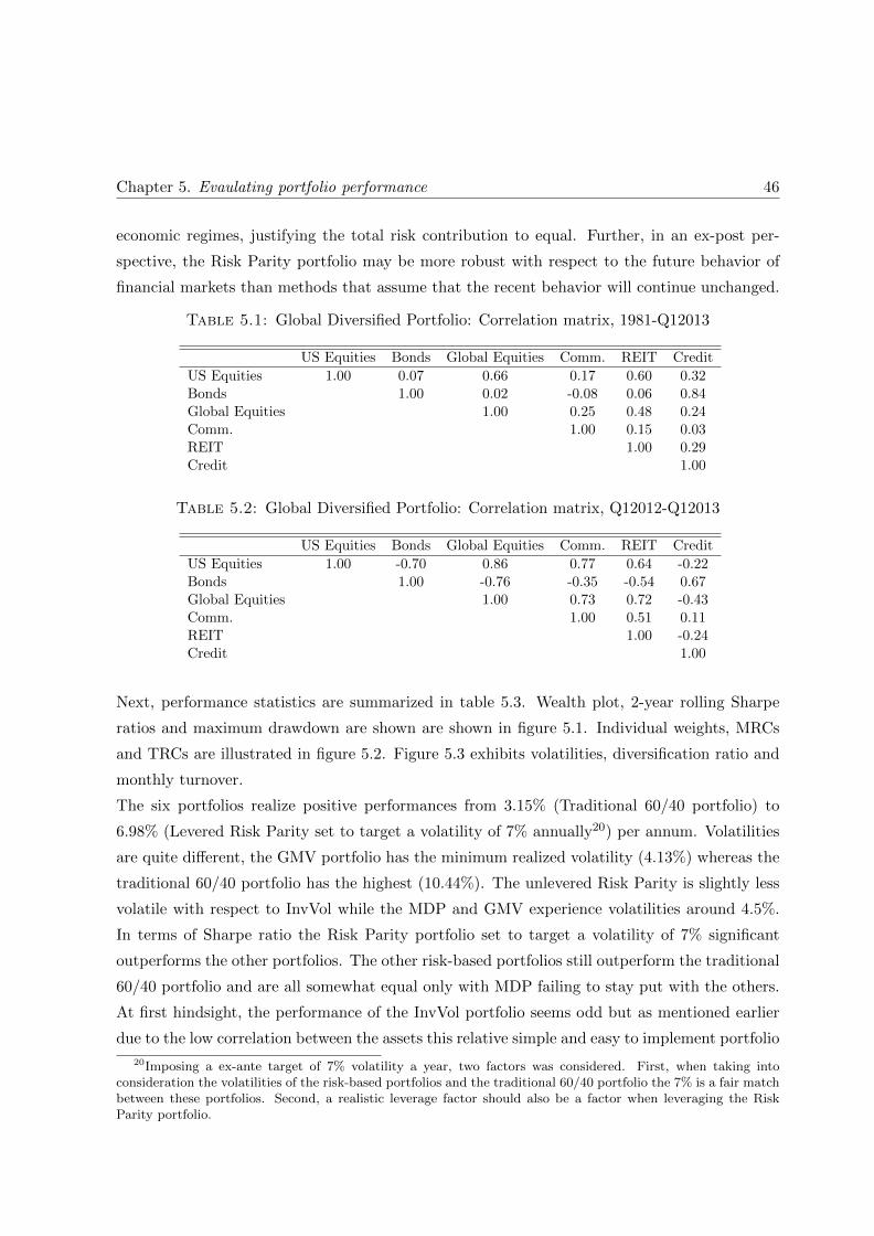
Chapter 5. Evaulating portfolio performance 46
economic regimes, justifying the total risk contribution to equal. Further, in an ex-post per-
spective, the Risk Parity portfolio may be more robust with respect to the future behavior of
financial markets than methods that assume that the recent behavior will continue unchanged.
Table 5.1: Global Diversified Portfolio: Correlation matrix, 1981-Q12013
US Equities Bonds Global Equities Comm. REIT Credit
US Equities 1.00 0.07 0.66 0.17 0.60 0.32Bonds 1.00 0.02 -0.08 0.06 0.84Global Equities 1.00 0.25 0.48 0.24Comm. 1.00 0.15 0.03REIT 1.00 0.29Credit 1.00
Table 5.2: Global Diversified Portfolio: Correlation matrix, Q12012-Q12013
US Equities Bonds Global Equities Comm. REIT Credit
US Equities 1.00 -0.70 0.86 0.77 0.64 -0.22Bonds 1.00 -0.76 -0.35 -0.54 0.67Global Equities 1.00 0.73 0.72 -0.43Comm. 1.00 0.51 0.11REIT 1.00 -0.24Credit 1.00
Next, performance statistics are summarized in table 5.3. Wealth plot, 2-year rolling Sharpe
ratios and maximum drawdown are shown are shown in figure 5.1. Individual weights, MRCs
and TRCs are illustrated in figure 5.2. Figure 5.3 exhibits volatilities, diversification ratio and
monthly turnover.
The six portfolios realize positive performances from 3.15% (Traditional 60/40 portfolio) to
6.98% (Levered Risk Parity set to target a volatility of 7% annually20) per annum. Volatilities
are quite different, the GMV portfolio has the minimum realized volatility (4.13%) whereas the
traditional 60/40 portfolio has the highest (10.44%). The unlevered Risk Parity is slightly less
volatile with respect to InvVol while the MDP and GMV experience volatilities around 4.5%.
In terms of Sharpe ratio the Risk Parity portfolio set to target a volatility of 7% significant
outperforms the other portfolios. The other risk-based portfolios still outperform the traditional
60/40 portfolio and are all somewhat equal only with MDP failing to stay put with the others.
At first hindsight, the performance of the InvVol portfolio seems odd but as mentioned earlier
due to the low correlation between the assets this relative simple and easy to implement portfolio
20Imposing a ex-ante target of 7% volatility a year, two factors was considered. First, when taking intoconsideration the volatilities of the risk-based portfolios and the traditional 60/40 portfolio the 7% is a fair matchbetween these portfolios. Second, a realistic leverage factor should also be a factor when leveraging the RiskParity portfolio.

Chapter 5. Evaulating portfolio performance 47
strongly benefits in this investment universe and its performance closely follows the unlevered
Risk Parity together with the advantage of much lower turnover.
Looking at maximum drawdown, diversification ratio and turnover one could argue that the
traditional 60/40 portfolio and the levered Risk Parity portfolio are risky portfolios whereas the
four others are more prudent portfolios. Especiallt during market crisis, i.e. the burst of the dot-
com bubble in early 2000 or the failure of Lehman Brothers during the recent financial crisis, the
two portfolios suffered extreme losses. As expected, risk-based portfolios lead to portfolios with
significant higher diversification, measured by the diversification ratio. The traditional 60/40
portfolio experience a yearly diversification of 1.35% whereas the MDP offers 3.22% implying
that a investor with a 60/40 allocation strategy misses out on the opportunity to effectively
diversify. Although the theory suggets the MDP to hold the highest diversification ratio, as a
surprise, the GMV portfolio actually offers slightly better diversification effect than the MDP.
However, as seen later on, this stricking result probably is affected by the investment universe
more than it is an anomaly.
Table 5.3: Global Diversified Portfolio statistics, 1981-Q12013
60/40 InvVol MDP GMV RP LRP (7%)
Excess return ann. (%) 3.15 4.23 3.42 3.35 4.16 6.98Volatility ann. (%) 10.44 5.79 4.86 4.13 5.36 7.00Sharpe Ratio 0.30 0.73 0.70 0.81 0.77 1.00MDD (%) 37.86 21.03 14.11 12.24 19.12 34.36Diversification Ratio ann. (%) 1.35 2.83 3.22 3.34 3.05 3.05Turnover ann. (%) 0.24 2.76 11.06 9.38 4.69 8.98
Note: The analysis stems from monthly returns and the backtest setup is done by usingmonthly rebalancing and an historical estimation period of 24 months. All results are appliedusing Matlab. Source: Bloomberg
As table 5.3 reveals, the levered Risk Parity yields the highest risk-adjusted performance in
terms of Sharpe ratio comparison. While both Risk Parity portfolios benefits from their well
diversified portfolio regarding total risk contribution, the unlevered Risk Parity portfolio is
beaten by the GMV, showing an superior Sharpe ratio of 0.81. An parameter measuring the
costs of rebalancing in order to construct each optimal portfolio is applied, namely the turnover.
Figure 5.3 shows the turnover for all portfolios at each rebalancing whereas table 5.3 exhibits
the annualized turnover to get a sense of the amount of trading required to implement each
portfolio strategy. Whereas the traditional 60/40 portfolio naturally profits from low turnover
both the MDP and GMV portfolio suffer from high turnover leading them to costly portfolios to
pursue. The transaction costs in the levered Risk Parirty portfolio is also high reflected by the
high turnover which indicates that it requires persistent trading throughout the sample period.

Chapter 5. Evaulating portfolio performance 48
In figure 5.1 one can observe the portfolios wealth composition over time. Again, the distinction
between the risky portfolios and more prudent are easy to see. Clearly, the MDP, GMV,
InvVol and unlevered Risk Parity are the most stable portfolios with the two latter realizing a
better performance over the sample period. This relative noteworthy drag in MDP and GMV’s
performance might be related to the allocation of the different asset classes in the portfolios.
Looking at figure 5.2 one can note that both portfolios are highly concentrated in few assets
and even though it is the unique characteristic within these two portfolios a deeper analysis in
applying constraints on the maximum holding of each assets would perhaps explain some of this
underperformance.
Turning to figure 5.2 and recalling the theoretical properties of the risk-based portfolios from
table 4.1 a few remarks should be made. First, pursuing the traditional 60/40 portfolio which
is diversified in terms of capital one cannot question the fact that more than 80% of the risk (in
volatile periods, such as in early 2000 and during the recent financial crisis, approximately 100%
of the total risk in the portfolio appeared from equities) in this portfolio occurs from equities.
Second, the GMV portfolio which features the MRCs to be equal experiences some distortions
and are not equal throughout the sample period. However, it is still the portfolio which equalize
MRCs the most. Additional, during several periods within the sample period both the MDP and
GMV portfolios experience extreme allocations with the result of only holding a minor fraction
of the asset classes represented. Third, both the unlevered and levered Risk Parity portfolio
yield equal TRCs with only minor distortion in two highly volatile periods. Throughout 2004-
2005 and again in 2008-2009 it indicates that the SQP algorithm is falling short of its ability
to optimize the weights. Furthermore, the levered Risk Parity porfolio’s average leverage factor
throughout the sample period is 1.4x with leverage reaching above 2.0x during the last years.
Table 5.4 summarizes key aspects of the two Risk Parity portfolios versus the traditonal 60/40
portfolio. Again, a few highlights stand out in this table. One is that the levered Risk Parity
portfolio has outperformed the traditional 60/40 portfolio in 20 out of past 33 years and by a
significant margin (wich is confirmed in figure 5.1 as well). Another note is that the volatility
of the traditional 60/40 portfolio has only been less than the 7% targeted by the levered Risk
Parity portfolio in four out of the 33 years. Based on this, it is likely that an investor choosing
the Risk Parity portfolio can choose the lowest risk-profile while still significantly outperform
the traditional 60/40 portfolio when a relative leverage factor is applied.

Chapter 5. Evaulating portfolio performance 49
Figure 5.1: Global Diversified Portfolio: Performance, 1981-Q12013
(a) Wealth Plot
(b) 2-year rolling Sharpe ratio
(c) 2-year rolling Maximum Drawdown

Chapter 5. Evaulating portfolio performance 50
Figure 5.2: Global Diversified Portfolio: Risk Factors, 1981-Q12013
(a) Individual weights
(b) Marginal Risk Contribution (MRC)
(c) Total Risk Contribution (TRC)
Note: Upper left (Traditional 60/40), upper middle (Inverse Volatility), upper right (Maximum Diversification),lower left (Global Minimum Variance), lower middle (Risk Parity) and lower right (Levered Risk Parity)

Chapter 5. Evaulating portfolio performance 51
Figure 5.3: Global Diversified Portfolio: Statistics, 1981-Q12013
(a) Yearly volatility
(b) Diversification ratio
(c) Monthly turnover

Table 5.4: Traditional 60/40 portfolio versus unlevered Risk Parity and levered Risk Parity’s volatility and returns.Risk Parity implied leverage factor and Risk Parity weights for each asset class, 1981-Q12013
60/40 σ RP σ LRP σ 60/40 (%) RP (%) LRP (%) L-factor Equities Bonds EM Equities Comm. REIT Credit
1981 11.6 11.1 7.0 -9.9 -12.5 -0.9 0.66 14 [14] 29 [31] 13 [16] 13 [16] 13 [15] 18 [15]1982 11.8 9.2 7.0 -10.3 1.5 4.2 0.79 13 [15] 24 [31] 12 [17] 20 [26] 16 [21] 15 [19]1983 11.9 8.4 7.0 8.9 6.5 5.1 0.84 12 [15] 23 [36] 10 [18] 27 [40] 13 [19] 14 [21]1984 9.6 5.8 7.0 0.6 1.9 1.1 1.21 10 [12] 28 [34] 9 [10] 27 [33] 11 [13] 16 [19]1985 9.7 5.4 7.0 24.0 10.4 13.8 1.31 8 [11] 26 [35] 10 [13] 22 [29] 16 [21] 18 [23]1986 10.8 6.0 7.0 22.4 13.8 18.0 1.17 9 [10] 22 [25] 11 [13] 17 [20] 21 [24] 20 [24]1987 11.8 6.6 7.0 9.3 4.3 4.7 1.06 9 [10] 22 [23] 10 [10] 15 [16] 17 [18] 26 [28]1988 12.6 5.9 7.0 10.9 6.4 6.7 1.25 8 [10] 29 [37] 6 [8] 17 [22] 10 [12] 29 [37]1989 10.7 4.2 7.0 1.3 8.2 12.3 1.71 8 [13] 27 [47] 68 [11] 22 [38] 10 [17] 26 [45]1990 12.2 4.4 7.0 -11.9 -0.5 -8.7 1.57 7 [11] 23 [37] 9 [13] 20 [31] 18 [28] 24 [37]1991 16.0 4.8 7.0 3.5 9.4 15.6 1.47 8 [11] 26 [38] 8 [12] 18 [26] 15 [21] 26 [37]1992 14.5 4.5 7.0 -8.6 2.8 4.5 1.60 8 [12] 27 [44] 8 [13] 18 [29] 12 [20] 27 [43]1993 10.3 4.4 7.0 20.7 9.0 19.3 1.58 7 [12] 24 [38] 12 [19] 23 [36] 10 [15] 24 [47]1994 10.7 5.5 7.0 0.1 -5.7 -10.3 1.28 9 [11] 24 [30] 18 [23] 15 [19] 11 [14] 22 [28]1995 9.8 5.9 7.0 -0.5 7.8 9.7 1.18 10 [12] 26 [31] 14 [17] 14 [17] 13 [16] 22 [26]1996 6.8 4.8 7.0 2.1 8.9 14.5 1.49 12[19] 24 [36] 14 [20] 12 [19] 13 [20] 23 [35]1997 6.5 4.6 7.0 0.9 10.1 19.9 1.51 12 [19] 25 [38] 11 [16] 11 [17] 17 [26] 23 [35]1998 8.6 5.1 7.0 5.2 -2.7 -8.2 1.37 10 [14] 33 [45] 8 [11] 11 [15] 13 [17] 26 [35]1999 10.1 5.1 7.0 6.9 -1.4 -4.7 1.41 10 [14] 41 [59] 6 [9] 7 [10] 9 [12] 26 [37]2000 9.7 4.6 7.0 -4.2 3.7 1.7 1.54 9 [14] 37 [57] 7 [10] 7 [10] 12 [18] 29 [44]2001 9.3 3.8 7.0 -15.6 1.8 -2.5 1.92 7 [12] 32 [61] 6 [12] 8 [16] 15 [29] 32 [62]2002 9.0 3.5 7.0 -7.7 2.7 6.5 1.99 6 [12] 33 [66] 7 [14] 7 [14] 14 [27] 34 [67]2003 9.7 4.1 7.0 13.8 12.1 36.2 1.71 7 [12] 38 [65] 10 [16] 7 [11] 13 [22] 25 [43]2004 9.4 5.5 7.0 10.2 12.5 22.5 1.27 10 [13] 30 [38] 14 [17] 11 [14] 11 [14] 24 [30]2005 7.0 5.0 7.0 6.5 4.6 9.4 1.43 12 [17] 25 [36] 16 [23] 12 [17] 9 [12] 25 [36]2006 6.2 4.0 7.0 10.8 4.9 7.3 1.84 11 [19] 30 [55] 14 [25] 8 [14] 8 [15] 30 [56]2007 5.4 3.6 7.0 9.9 4.2 9.4 1.96 11 [21] 30 [59] 14 [27] 8 [13] 8 [16] 30 [60]2008 7.0 3.4 7.0 -35.4 -10.8 -38.5 2.00 8 [16] 40 [77] 10 [20] 7 [14] 6 [13] 29 [61]2009 15.2 7.7 7.0 17.3 9.6 8.7 1.07 6 [6] 50 [52] 8 [8] 7 [7] 4 [6] 15 [17]2010 16.8 8.2 7.0 7.1 9.4 7.2 1.11 6 [7] 51 [54] 6 [8] 7 [9] 4 [5] 19 [20]2011 11.7 4.2 7.0 -0.9 5.3 19.5 1.82 5 [8] 56 [103] 6 [10] 6 [11] 5 [9] 22 [39]2012 11.7 3.1 7.0 3.0 5.3 28.3 2.31 4 [10] 65 [149] 5 [15] 6 [10] 4 [9] 16 [38]Q12013 11.2 3.0 7.0 5.2 3.9 11.3 2.53 5 [12] 64 [163] 7 [17] 4 [10] 4 [10] 16 [41]
Note: The levered Risk Parity weights are shown in the brackets
52

Chapter 5. Evaulating portfolio performance 53
5.4 Global Portfolios
The second backtest steems from the analysis of global asset classes. Whereas the previous
investment universe was highly uncorrelated, this analysis is based on a broader range of global
asset classes as well as the asset classes feature a higher degree of correlation.
The investment universe is a combination of equities, bonds, commodities, real estate and credit.
As such, the risky assets are:
• S&P 500 Total Return Index (US Equities)
• Russel 3000 Total Return Index (US equities)
• MSCI EAFE Total Return Index (Global equities)
• MSCI Daily EM Total Return Index (Emerging Market equities)
• Barclays Aggregate Bond Total Return Index (Global bonds)
• J.P. Morgan Global Aggregate Bond Index (Global bonds)
• S&P GSCI Total Return Index (Commodities)
• Dow Jones UBS Commodity Total Return Index (Commodities)
• FTSE REIT Total Return Index (Real Estate)
• Barclays US Corporate High Yield Total Return Index (HY Credit)
• Barclays US Aggregate Credit Total Return Index (Credit)
• Merill Lynch US High Yield Total Return Index (HY Credit)
All the above mentioned asset classes are represented in USD. The sample period stems from
January 1999 to March 2013 using daily returns. For this analysis the first 24 months are used
to construct the very first portfolio, so portfolio returns start in January 2001. The 1-month
LIBOR rate is used as a proxy for the risk-free rate and therefore all excess returns are based
on returns excess of the 1-month LIBOR rate. When leveraging the Risk Parity portfolio, the
1-month Eurodollar Deposit rate is used as a proxy for cost of borrowing.

Chapter 5. Evaulating portfolio performance 54
Table 5.5: Global Portfolio: Correlation matrix, 2001-Q12013
Globalequi-ties
AllUS
equi-ties
S&P500
EMequi-ties
BCGlobalbonds
JPMGlobalbonds
GSCIComm.
REITUS
Corp.HY
UBSComm.
USAgg.credit
USAgg.HY
Global equities 1.00 0.50 0.49 0.78 0.03 0.22 0.36 0.28 0.45 0.42 -0.08 0.48All US equities 1.00 1.00 0.45 -0.22 -0.12 0.26 0.74 0.21 0.27 -0.28 0.23S&P 500 1.00 0.44 -0.22 -0.13 0.26 0.73 0.20 0.26 -0.28 0.22EM equities 1.00 -0.05 0.07 0.36 0.30 0.47 0.41 -0.07 0.50BC Global bonds 1.00 0.68 -0.01 -0.13 0.08 0.01 0.67 0.07JPM Global bonds 1.00 0.10 -0.06 0.07 0.14 0.52 0.06GSCI Comm. 1.00 0.17 0.18 0.91 -0.12 0.18REIT 1.00 0.11 0.17 -0.18 0.11US Corp. HY 1.00 0.22 0.18 0.89UBS Comm. 1.00 -0.11 0.23US Agg. credit 1.00 0.20US Agg. HY 1.00
As intended, the following correlation analysis for the total period from January 2001 through
March 2013 in table 5.5 confirms the investment universe to be more correlated than in the
previous findings based on a set of global diversified asset classes. Furthermore, turning to table
5.6 verifies correlations to be more stable across different economic regimes. More interestingly,
the index issued by Barclays representing US aggregate credit experiences negative correlation
with all other indicies except bonds. In addition, during the last year the correlations for this
index seem to be reaching significant levels. This might indicates that some asset rotation
between equities and credit occurs.
Table 5.7 exhibits the annualized return of the traditional 60/40 portfolio which amounts to
4.05% at a volatility of 10.07% which implies a Sharpe ratio of 0.40. Among the risk-based
Table 5.6: Global Portfolio: Correlation matrix, Q12012-Q12013
Globalequi-ties
AllUS
equi-ties
S&P500
EMequi-ties
BCGlobalbonds
JPMGlobalbonds
GSCIComm.
REITUS
Corp.HY
UBSComm.
USAgg.credit
USAgg.HY
Global equities 1.00 0.61 0.61 0.79 -0.07 0.37 0.51 0.40 0.62 0.47 -0.33 0.61All US equities 1.00 1.00 0.51 -0.22 0.08 0.51 0.71 0.40 0.40 -0.54 0.37S&P 500 1.00 0.50 -0.21 0.08 0.50 0.70 0.40 0.39 -0.54 0.37EM equities 1.00 -0.12 0.22 0.49 0.38 0.60 0.46 -0.29 0.58BC Global bonds 1.00 0.68 -0.11 -0.08 -0.02 -0.01 0.71 0.01JPM Global bonds 1.00 0.21 0.10 0.16 0.24 0.40 0.16GSCI Comm. 1.00 0.28 0.27 0.86 -0.31 0.27REIT 1.00 0.33 0.23 -0.29 0.29US Corp. HY 1.00 0.31 -0.14 0.99UBS Comm. 1.00 -0.20 0.28US Agg. credit 1.00 -0.12US Agg. HY 1.00

Chapter 5. Evaulating portfolio performance 55
portfolios there are some stricking results. The range regarding volatilities are from 10.07%
(Levered Risk Parity set to target the volatility of the traditional 60/40 portfolio) to 3.03%
(GMV). Likewise, the range of annualized return is quite large. The levered Risk Parity has
returned the most (8.31%) and GMV is the only portfolio with a lower return than the traditional
60/40 portfolio. However, taking a closer look at the risk-adjusted figures, one has to note that
investing in the GMV portfolio entails significant outperformance of all the other portfolios.
Again, the InvVol portfolio delievers great performance despite its simple allocatoin scheme.
One driver for this impressive Sharpe ratio (0.80) is the overweight into the US Aggregate Credit
index issued by Barclays, producing a historical 6.28% return with 5.06% volatility, implying
a Sharpe ratio of 1.24. Only the Merrill Lynch US High Yield index produces a higher Sharpe
ratio (1.50). As the levered Risk Parity portfolio is set to target the volatility of the traditional
60/40 portfolio the Sharpe ratio of this portfolio is affected by this, resulting in a Sharpe ratio
of 0.83 which still is below the ones acquired by the MDP and GMV portfolios.
Turning to maximum drawdown in table 5.7 the unlevered Risk Parity portfolio do not seems
to favor more of the lower-risk asset classes, which would predict in one the lowest downside-
risk portfolios. As already highlighted, the volatility is higher than any of the other risk-based
portfolios and when taking a closer look at the downside-risk of the portfolio it closely follows
the traditional 60/40 portfolio. Moreover, the levered Risk Parity portfolio exhibits the highest
drawdown (48.64%) which is relatively high when compared to the 23.90%, 24.07% and 28.38%
of the GMV, MDP and InvVol portfolios, respectively. In the previous findings, the GMV
portfolio obtained higher diversification effects than any of the other portfolios but in this
backtest, the MDP portfolio confirms the theory by being the most diversified portfolio, in
terms of diversification ratio. When turning the attention to the diversification ratio of the
traditional 60/40 portfolio it may be a stricking point that it produces diversification effects
close to the risk-based portfolios which features complex optimization schemes. However, as the
traditional 60/40 portfolio is divided into various sub-asset classes within equities and bonds
together with equities and bonds experience negative correlation, thereby providing implicit
diversification effects, this might provide some of the explanation.
Note that the levered Risk Parity entails the largest turnover among all portfolios with 13.78%
suggesting that transacion costs may reduce the relative return potential while MDP has a
turnover of 12.00%, which is comparable to the one of GMV (12.36%). In light of this and taking
into account possible reduction in actual realized performance, the InvVol and unlevered Risk
Parity might be better alternative based on their low turnover (8.00% and 8.56%, respectively).
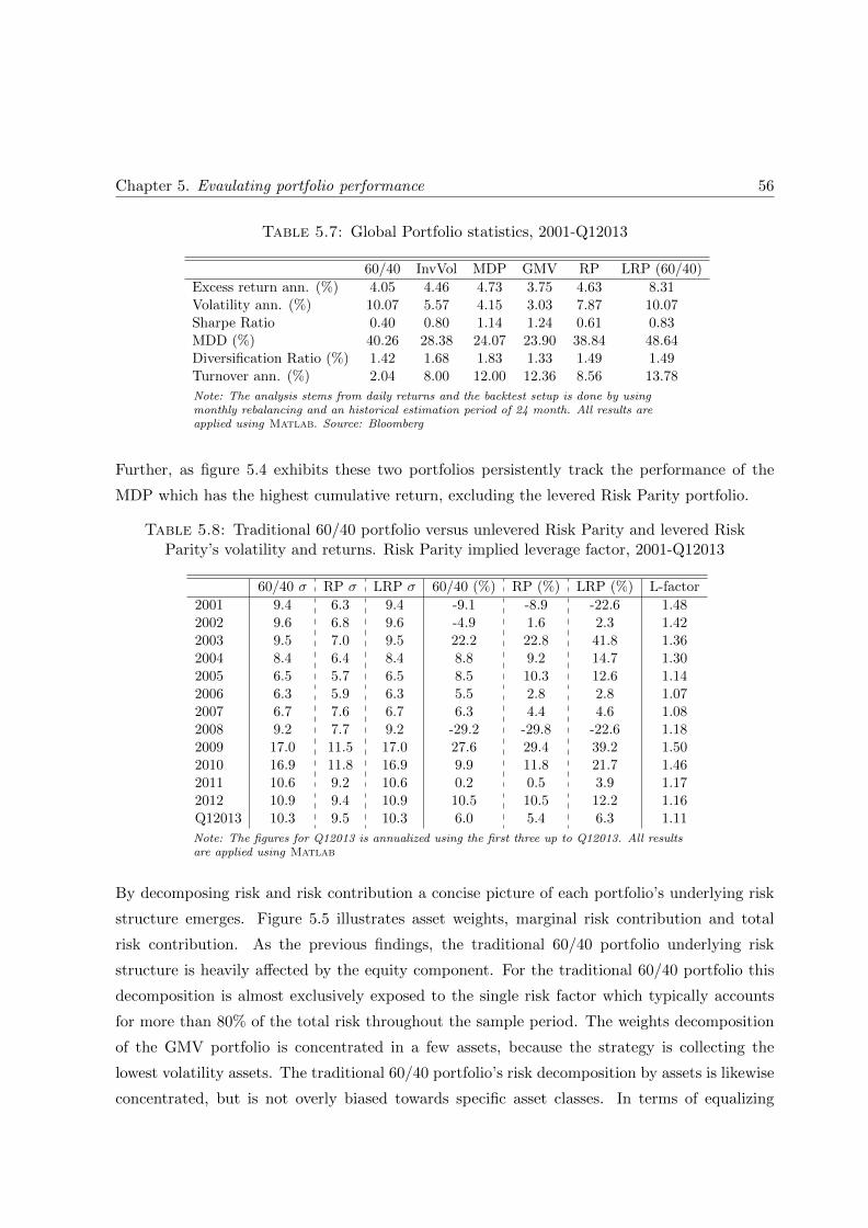
Chapter 5. Evaulating portfolio performance 56
Table 5.7: Global Portfolio statistics, 2001-Q12013
60/40 InvVol MDP GMV RP LRP (60/40)
Excess return ann. (%) 4.05 4.46 4.73 3.75 4.63 8.31Volatility ann. (%) 10.07 5.57 4.15 3.03 7.87 10.07Sharpe Ratio 0.40 0.80 1.14 1.24 0.61 0.83MDD (%) 40.26 28.38 24.07 23.90 38.84 48.64Diversification Ratio (%) 1.42 1.68 1.83 1.33 1.49 1.49Turnover ann. (%) 2.04 8.00 12.00 12.36 8.56 13.78
Note: The analysis stems from daily returns and the backtest setup is done by usingmonthly rebalancing and an historical estimation period of 24 month. All results areapplied using Matlab. Source: Bloomberg
Further, as figure 5.4 exhibits these two portfolios persistently track the performance of the
MDP which has the highest cumulative return, excluding the levered Risk Parity portfolio.
Table 5.8: Traditional 60/40 portfolio versus unlevered Risk Parity and levered RiskParity’s volatility and returns. Risk Parity implied leverage factor, 2001-Q12013
60/40 σ RP σ LRP σ 60/40 (%) RP (%) LRP (%) L-factor
2001 9.4 6.3 9.4 -9.1 -8.9 -22.6 1.482002 9.6 6.8 9.6 -4.9 1.6 2.3 1.422003 9.5 7.0 9.5 22.2 22.8 41.8 1.362004 8.4 6.4 8.4 8.8 9.2 14.7 1.302005 6.5 5.7 6.5 8.5 10.3 12.6 1.142006 6.3 5.9 6.3 5.5 2.8 2.8 1.072007 6.7 7.6 6.7 6.3 4.4 4.6 1.082008 9.2 7.7 9.2 -29.2 -29.8 -22.6 1.182009 17.0 11.5 17.0 27.6 29.4 39.2 1.502010 16.9 11.8 16.9 9.9 11.8 21.7 1.462011 10.6 9.2 10.6 0.2 0.5 3.9 1.172012 10.9 9.4 10.9 10.5 10.5 12.2 1.16Q12013 10.3 9.5 10.3 6.0 5.4 6.3 1.11
Note: The figures for Q12013 is annualized using the first three up to Q12013. All resultsare applied using Matlab
By decomposing risk and risk contribution a concise picture of each portfolio’s underlying risk
structure emerges. Figure 5.5 illustrates asset weights, marginal risk contribution and total
risk contribution. As the previous findings, the traditional 60/40 portfolio underlying risk
structure is heavily affected by the equity component. For the traditional 60/40 portfolio this
decomposition is almost exclusively exposed to the single risk factor which typically accounts
for more than 80% of the total risk throughout the sample period. The weights decomposition
of the GMV portfolio is concentrated in a few assets, because the strategy is collecting the
lowest volatility assets. The traditional 60/40 portfolio’s risk decomposition by assets is likewise
concentrated, but is not overly biased towards specific asset classes. In terms of equalizing

Chapter 5. Evaulating portfolio performance 57
MRCs, the GMV portfolio has some minor distortion and features a biased allocation into the
sub-asset class REIT. Nevertheless, its risk decomposition is more diverse than any of the other
portfolios in terms of MRC. Similar, figure 5.5 exhibits the Risk Parity portfolios to be the only
two portfolio truly diversified in terms of TRC. Again, the portfolios feature minor distortion
from the year 2009 until 2011 but this is probably due to a programming issue rather than a
input distortion.
The leverage required to obtain equal volatility as the traditional 60/40 portfolio is relatively
minor than in the previous findings. The average leverage factor during the sample period is
1.28x. Table 5.8 summarizes key aspects of the risk-return characteristics for the traditional
60/40 portfolio as well as for the two Risk Parity portfolios, in each year from 2001 until Q12013.
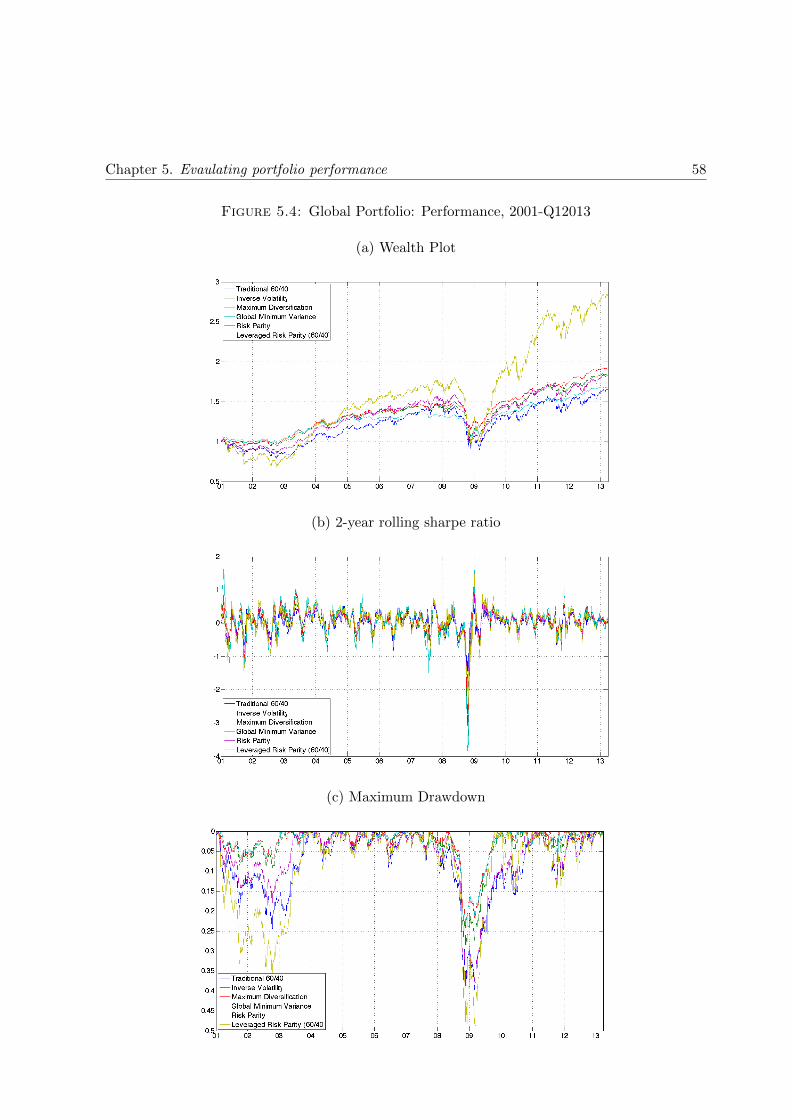
Chapter 5. Evaulating portfolio performance 58
Figure 5.4: Global Portfolio: Performance, 2001-Q12013
(a) Wealth Plot
(b) 2-year rolling sharpe ratio
(c) Maximum Drawdown

Chapter 5. Evaulating portfolio performance 59
Figure 5.5: Global Portfolio: Risk Factors, 2001-Q12013
(a) Individual weights
(b) Marginal Risk Contribution (MRC)
(c) Total Risk Contribution (TRC)
Note: Upper left (Traditional 60/40), upper middle (Inverse Volatility), upper right (Maximum Diversification),lower left (Global Minimum Variance), lower middle (Risk Parity) and lower right (Levered Risk Parity)

Chapter 5. Evaulating portfolio performance 60
Figure 5.6: Global Portfolio: Statistics, 2001-Q12013
(a) Monthly volatility
(b) Diversification ratio
(c) Daily turnover

Chapter 5. Evaulating portfolio performance 61
5.5 World Equity Sectors Portfolios
The last backtest is done upon the sub-asset class equity. Moreover, the investment universe
covers worldwide equity sectors. The fact that there is a lot of common, systematic risk across
equities should in theory suggests that the diversification potential within equities is limited.
As a result, the benefits in portfolio construction that produces high diversification with the
aim at generating better performance is examined in this backtest. This limitation in relying
only on equities is a mere practical one which will in no way diminish the results in this thesis.
Moreover, the risky assets are:
• Energy (Bloomberg: NDWUENR Index)
• Materials (Bloomberg: NDWUMAT Index)
• Industrial (Bloomberg: NDWUIND Index)
• Consumer Discretionary (Bloomberg: NDWUCDIS Index)
• Consumer Staples (Bloomberg: NDWUCSTA Index)
• Health Care (Bloomberg: NDWUHC Index)
• Financials (Bloomberg: NDWUFN Index)
• Telecommunications (Bloomberg: NDWUTEL Index)
• Utilities (Bloomberg: NDWUUTIL Index)
All the above mentioned asset classes are represented in USD. The sample period stems from
January 2001 to March 2013 using daily returns. For this analysis the first 24 months are used
to construct the very first portfolio, so portfolio returns start in January 2003. The 1-month
LIBOR rate is used as a proxy for the risk-free rate and therefore all excess returns are based
on returns excess of the 1-month LIBOR rate.
Backtest results are summarized in table 5.11, performance in figure 5.7, portfolio weights are
shown in figure 5.8 and statistics are illustrated in figure 5.9. The four portfolio strategies realize
positive performance from 6.18% (InvVol) to 7.94% (GMV) per annum. Volatilities are similar
due to the fact that the investment universe only contains equities. The GMV portfolio has
the minimum realized volatility (12.13%) and Risk Parity the highest (15.75%). Furthermore,

Chapter 5. Evaulating portfolio performance 62
Table 5.9: World Equity Sectors: Correlation matrix, 2003-Q12013
Energy Materials IndustrialConsumerDiscre-tionary
ConsumerStaples
HealthCare
FinancialsTele
commu-nications
Utilities
Energy 1.00 0.81 0.79 0.72 0.73 0.69 0.73 0.71 0.79Materials 1.00 0.88 0.79 0.72 0.65 0.79 0.73 0.76Industrial 1.00 0.93 0.83 0.77 0.90 0.79 0.78Consumer Discretionary 1.00 0.83 0.76 0.86 0.79 0.73Consumer Staples 1.00 0.84 0.78 0.82 0.82Health Care 1.00 0.73 0.76 0.77Financials 1.00 0.78 0.73Telecommunications 1.00 0.80Utilities 1.00
correlations during the whole sample period (see table 5.9) show that all indicies are highly
correlated and contribute to the hypothesis of the high systematic risk associated with investing
in equities.
A stricking feature of the Global Minimum-Variance portfolio constructed subject to the re-
striction that portfolio weights should be nonnegative is that investment is spread over only a
few sectors (see table 5.8). The GMV portfolio of a 9-sector universe has between 1-3 sectors,
depending on the sample period. The annulized standard deviation of the return on the GMV
portfolio using the sample covariance matrix and 24 months of observations on returns with
monthly rebalancing is 12.13%. In contrast, the return on the unlevered Risk Parity portfolio
which containts all the 9 sectors in the universe has a standard deviation of 15.75%, that is 1.3
times as large. The GMV portfolio also has a higher Sharpe ratio (0.65) than the unlevered
Risk Parity strategy (0.44). While the describtive statistics on a portfolio of 3 randomly picked
sectors are unknown, it seems there is little incremental benefit to both naive and more optimal
diversification beyond 3 sectors. The single most important driver for the performance of the
Table 5.10: World Equity Sectors: Correlation matrix, Q12012-Q12013
Energy Materials IndustrialConsumerDiscre-tionary
ConsumerStaples
HealthCare
FinancialsTele
commu-nications
Utilities
Energy 1.00 0.89 0.91 0.88 0.85 0.87 0.89 0.83 0.81Materials 1.00 0.92 0.88 0.80 0.82 0.90 0.81 0.78Industrial 1.00 0.96 0.88 0.90 0.95 0.86 0.84Consumer Discretionary 1.00 0.87 0.89 0.91 0.82 0.82Consumer Staples 1.00 0.92 0.85 0.87 0.87Health Care 1.00 0.87 0.86 0.86Financials 1.00 0.86 0.85Telecommunications 1.00 0.89Utilities 1.00

Chapter 5. Evaulating portfolio performance 63
GMV portfolio is the allocation into Consumer Staples producing an annulized return of 8.47%
with volatility of only 12.81%, implying a Sharpe ratio of 0.66 which is more than 1.5x more
than the second best risk-adjusted asset class (Materials has a Sharpe ratio of 0.43).
Having only 3 sectors in the GMV portfolio should raise some concern. Variance is an adequate
measure of risk of returns that have a normal distributoin. The return on a portfolio of a large
collection of asset classes will, in general, be close enough to a normal distribution to justify
the use of variance as the measure of risk. This may not be true for a portfolio holding only
3 sectors. In particular, the probability of an extreme event, may be substantially higher than
that computed by assuming a normal distribution. Imposing upper bounds on portfolio weights
would be one way to ensure that optimal portfolios will contain, in this example, a sufficiently
large collection of equitiy sectors.
Table 5.11: World Equity Sectors statistics, 2003-Q12013
InvVol MDP GMV RP
Excess return ann. (%) 6.18 6.60 7.94 6.82Volatility ann. (%) 15.37 15.53 12.13 15.75Sharpe Ratio 0.39 0.42 0.65 0.44MDD (%) 54.42 53.70 43.99 55.88Diversification Ratio (%) 1.48 1.51 1.34 1.46Turnover ann. (%) 8.59 12.06 10.80 8.64
Note: The analysis stems from daily returns and the backtest setup isdone by using monthly rebalancing and an historical estimation period of24 months. All results are applied using Matlab. Source: Bloomberg
In table 5.11, turning to maximum drawdown, all portfolios experience similiar drawdowns which
again advocates for a significant degree of systematic risk, regardless of the portfolio optimiza-
tion scheme. As expected the GMV portfolio has the minimum drawdown (43.99%) during
the sample period. Further, as the theory suggests, the MDP holds the most diversification
effect however not as substantial as in the two previous studies. Regarding turnover, in spite of
having only three sectors in the portfolio, the GMV strategy still suffers from a highly dynamic
allocation within these three sectors thereby implicit having a high turnover (10.80%) in com-
parison with the InvVol and Risk Parity portfolios which both require an annulized turnover of
approximately 8.60%. At the expense of having almost all sectors in the portfolio together with
a dynamic allocation at each rebalancing, the MDP has the highest turnover which indicates
that it may have the highest transaction costs imbedded in the strategy.

Chapter 5. Evaulating portfolio performance 64
Figure 5.7: World Equity Sectors: Performance, 2003-Q12013
(a) Wealth Plot
(b) 2-year rolling sharpe ratio
(c) Maximum Drawdown

Chapter 5. Evaulating portfolio performance 65
Figure 5.8: World Equity Sectors: Risk Factors, 2003-Q12013
(a) Individual weights
(b) Marginal Risk Contribution (MRC)
(c) Total Risk Contribution (TRC)
Note: Upper left (Inverse Volatility), upper right (Maximum Diversification), lower left (Global MinimumVariance), lower right (Risk Parity)

Chapter 5. Evaulating portfolio performance 66
Figure 5.9: World Equity Sectors: Statistics, 2003-Q12013
(a) Yearly volatility
(b) Diversification ratio
(c) Daily turnover

Part III
Robustness of Risk Parity
67

Chapter 6
The impact of biases in Asset
Allocation
Theories improve our understanding of life and often use algebra to do so. This algebra must be
error free. Yet that alone is not a prerequisite for a decent theory. Using optimization schemes
to find the right asset mix it not so different. History recognises the ingenuity and accuracy of
the supporting algebra. By such, investors want to find the asset mix that is optimal for us.
Yet the assumptions that an optimiser uses can quickly lead one into trouble.
When Markowitz introduced a cornerstone in modern finance with his article on portfolio selec-
tion theory he examined investors’ view on risk and return. He assumed that investors would
solely base their portfolio formation on mean-variance analysis, maximizing the relationship
between expected return and the associated risk. The mean-variance analysis was based on the
assumption that capital markets are frictionless, i.e. investors are able to buy and sell all assets
at competitive market prices without transaction costs.
Yet this framework has a well-known problem: the risk of the portfolios constructed in this
context is undererstimated, leading to a mismatch between ex-ante and ex-post risk of optimal
portfolios. The fact that an excellent risk model exhibits considerable risk bias on an optimized
portfolio is a long-time concern for practitioners who use the mean-variance optimization frame-
work to construct or rebalance their portfolios. The risk-minimizing optimization is a selection
process that biases in those securities more subject to risk underestimation.
68

Chapter 6. Will my Risk Parity strategy actually outperform? 69
6.1 Pitfalls of backtesting
Many dimensions of a portfolio strategy are not captured by the performance statistics desribed
so far. For example, market capacity affects the portfolio through the effect of position size on
future returns, which contradicts the implicit assumption held in the optimization scheme for
each portfolio. In practice, acquiring a large position may adversely affect the price at which it is
acquired and, hence, its future returns. Therefore, portfolio weights depend on the portfolio size,
making size an additional parameter in the portfolio construction process. Ideally, an investor
balances the effect of size versus maximizing the risk-adjusted performance thus the real-life
portfolio is a combination of the market portfolio and the optimal portfolio, where the latter is
the portfolio that maximizes performances versus risk disregarding size. Another critical issue
when constructing portfolios is the choice of constraints. In this thesis, the only constraint
used is the limitation of nonnegative weights allowing for long-only portfolios. By adding other
constraints, such as an upper bound of the maximum holding in each asset class, may favor the
overall portfolio performance as well as reduce the likelihood of extreme allocation into a few
asset classes. In addition, by easing the nonnegative constraint one could also allow an investor
to short an asset class. However, a problem in measuring the risk contribution in percentage
can arise for long-short portfolios. For example, suppose a long position matches perfectly the
short position in terms of capital. In this case, the value of the portfolio is zero and the relative
risk constribution is infinite. Furthermore, a concern is hightened when a proposed portfolio
strategy is backtested by using historical data. Consider an investment strategy that can be
pursued today with readily available securities. If those securities were unavailable in the past,
then the strategy has no true antecedent. Backtesting must be conducted with proxies for the
securities, and the choice of proxies can have a direct effect on measured returns.
In addition to trading size, constraints and investment universe, several and more general bi-
ases arise when an investor backtest a portfolio strategy. These biases will be elabroated and
discussed for the rest of this section by using the investment universe as in section 5.3 and only
focusing on the wealth performance of each strategy21.
21Only focusing on the wealth performance is not a truly holistic analysis. In order to make a deeper analysisone should include the same performance measures as done in the studies applied in chapter 5. However, due tothe scope of this thesis the wealth performance is choosen to represent the overall measure of the performance ofeach portfolio strategy

Chapter 6. Will my Risk Parity strategy actually outperform? 70
6.1.1 Rebalancing
A portfolio’s asset allocation is the major determinant of a portfolio’s risk/return characteris-
tics. Yet, as time passes, asset classes produce different returns so the portfolio’s asset allocation
changes. As a consequence, to recapture the portfolio’s optimal risk/return characteristics, the
portfolio should be rebalanced in order to minimize this suboptimality. The impact of rebal-
ancing is reported in figure C.1. The base setup used in this thesis is monthly rebalancing,
but in order to reflect on the choice of rebalancing two other choices are represented, namely
quaterly and yearly rebalancing. As the wealth plot exhibits, the choice of how frequent an
investor choices to rebalance the portfolio is not meaningfully different whether a portfolio is
rebalanced monthly, quaterly or annually. However, the imbedded costs can increase signifi-
cantly as the number of rebalancing increase. The levered Risk Parity portfolio, however, seems
to experience dramatical drags on the performance when rebalancing only quaterly or annualy.
The amount of excess return generated through rebalancing is a function of asset class volatility
and diversification. All else being equal, the more volatile and diversified the assets within a
portfolio, the more value that can be created through rebalancing. In the levered Risk Parity
portfolio, assets are selected based on their diversification benefits and thereafter levered to
achieve the target volatility of 7%. This construction scheme creates an ideal environment for
systematically harvesting gains in the portfolio through rebalancing frequently. However, when
rebalancing less frequently, this benefit seems to vanish.
6.1.2 Parameter estimation period
As mentioned regarding the choice of rebalancing, the choice of the most appropriate rolling
window or the period in estimating the parameters is very subjective. As chapter 5 describes,
the base setup is the use of two years (when daily data is used this corresponds to 520 days)
when estimating the volatilities and covariance matrices. However, as this is not an uniform
approach this rolling window is replaced by using one year (equivalent to 262 days) and five
years (equivalent to 1310). Figure C.2 exhibits the impact on these choices of rolling windows.
First, using one year to estimate the parameters all portfolios display the highest cumulative
wealth. Again, the levered Risk Parity portfolio signals significant benefits when much recent
data are applied instead of relying on a rolling window of five years. Similar, the GMV portfolio
entails a relative poor performance relative to the risk-based portfolios when using five years as
determinator for the parameters.

Chapter 6. Will my Risk Parity strategy actually outperform? 71
6.1.3 Cost of borrowing
As the robustness check is applied on the first backtest in chapter 5, the levered Risk Parity
portfolio is financed at the 1-month Eurodollar Deposit rate. In this subsection the study is
repeated by replacing the 1-month Eurodollar Deposit rate with the 90-days Treasury Bill rate
and the 3-month Eurodollar Deposit rate. This is shown in figure C.3.
By replacing the 1-month Eurodollar Deposit rate with the 90-days Treasury Bill the levered
Risk Parity portfolio has a slighly better performance, though, not a significant higher return.
Even though the 90-day Treasury Bill rate has a longer duration, it is considered less risky, all
else being equal, than the 1-month Eurodollar Deposit rate due to the fact that the T-Bill is
backed by the U.S. Government. As expected, when replacing the 1-month Eurodollar Deposit
rate with the 3-month Eurodollar Deposit rate when financing the levered Risk Parity portfolio,
the performance declines.
6.2 Pitfalls of Risk Parity
Past performance is not a guarantee of future returns. This familiar disclaimer highlights the
fact that a particular portfolio strategy may work well in some periods and poorly in others,
limiting the inference that can be drawn from past returns. Backtests typically performs better
than the real-world portfolio performance that is realized after the trade is put on. This is to
be expected for a number of reasons as discussed above.
With its appeal earned mostly by its superior performance in the past decade, the Risk Parity
portfolio also has its shortcomings. Admittedly, it has managed to perform exceptionally well
in different investment universes where other risk-based portfolios and the traditional 60/40
portfolio underperformed. However, the current market conditions during the last couple of
years may contributed to this superior outperformance where yields have been on a declining
path since the early 1980s. As such, this section highlights some drawbacks where the current
market conditions as well as critical assumptions in construction a Risk Parity portfolio are
reported.

Chapter 6. Will my Risk Parity strategy actually outperform? 72
6.2.1 Rising yields
In the current low-yield environment with a risk of rising yields it may not be advisable to build
a portfolio based on risk-balancing. Risk Parity advocates however claim that rising yields will
result in rising fixed income return volatility. According to these arguments, the approach will
then automatically reduce exposure to this asset class. During periods of spiking yields (for
example the notable sharp increase at the beginning of the 1980s) it follows that Risk Parity
portfolio seems to have managed to pull funds out of fixed income during such time22. The
paper shows that while the exposure to fixed income was at 81.9% in early 1979, applying
risk parity reduced this weight to as low as 45.6% in October 1981. As such, one can note
that periods of spiking yields are accompanied by spiking fixed income return volatility, hence
protecting investors by an improved portfolio composition during these periods unless equity
volatility increases simultaneously.
Figure 6.1: Robustness: Subperiods for Global Diversified Portfolios
(a) Base, 1981-Q12013 (b) Bull market, 1981-2000
(c) Last 10 years, 2003-Q12013 (d) Post financial crisis, 2009-Q12013
Figure 6.1 plots four different subperiods of the investment universe covered in section 5.3. As
mentioned in chapter 3 in section 3.3, interest rate rose sharply in the beginning of 1994 and
taking a closer look at the portfolio composition during that time (see figure 5.2) one can see
22Meyer, B. and Kramer, A., Commerzbank, Risk Parity, 2013

Chapter 6. Will my Risk Parity strategy actually outperform? 73
the same trend as Meyer and Kramer identified. The fixed income exposure during late 1993
until the end of 1994 was reduced from 33.5% to 21.2%. Yet, if an investor had entered a Risk
Parity strategy in late 1993 the performance would be significant worse than any of the other
portfolios.
Figure 6.1 exhibits four subperiods from the investment universe described in section 5.3. Taking
a closer look at the portfolio performances, it is stricking that during the bull market (1981-
2000), entering the traditional 60/40 portfolio would leave investors with higher cumulative
return than any of the unlevered strategies. Admittedly, the traditional 60/40 portfolio displays
much more volatility and experiences higher drawdowns during times of turmoil due to its
constant mix strategy. In addition, the traditional 60/40 portfolio signals performance in line
with the Risk Parity strategy and superior performance over the GMV and MDP portfolios
when focusing on the performance post the financial crisis (2009-Q12013). During gradually
recovery of financial markets both the GMV and MDP portfolios seem to miss out performance
because of their high concentration into a few asset classes whereas the Risk Parity and in
particular the InvVol portfolio benefits from much more diversification across the asset classes.
6.2.2 Leverage
The CAPM framework usually assumes both the return on the low volatility and the more
volatile asset to be higher than the risk-free rate. While this assumption holds in the long run,
there might be temporay, though not necessarily short, periods when it does not. In addition,
there may be times with even negative total returns. In such case, this would typically result
in a mirror-inverted efficient frontier, i.e. the higher the risk, the lower the return. While such
a scenario sounds rather theoretical, this thesis reveals that such periods have in fact occured a
few times during the past decades.
During 1994, the risk-free rate was approximately 4.5% while bonds and credits displayed both
negative excess returns as well as negative total returns. The traditional 60/40 portfolio had the
advantage of its allocation into equities during this period where equities exhibit positive excess
return. As table 5.4 in chapter 5 shows, while the traditional 60/40 portfolio generated an return
of 0.1% , the unlevered Risk Parity portfolio suffered a loss of 5.7%. However, levering up this
portfolio would have proved to be a bad decision. The levered Risk Parity portfolio returned an
annual loss of 10.3%, i.e. approximately twice the size of the loss of the unlevered Risk Parity
portfolio. In other words, when low volatile asset classes is declining in tandem, owning a levered

Chapter 6. Will my Risk Parity strategy actually outperform? 74
portfolio of such assets is substantially worse than owning these assets unlevered. Admittedly,
the period is very short. However, it shows and proves that even within short sample periods,
Risk Parity obtained by the use of leverage may fail miserably and can result in a strongly
negative performance.
6.2.3 Return distribution
As such, Risk Parity does not assume normally distributed returns. However, as this thesis has
analyzed Risk Parity and its underlying assumptions in the classical risk-return space, which
usually assumes normally distributed asset returns. Yet the performance of the Risk Parity
portfolio tends to suffer from the fact that returns are not normally distributed. The 2008
financial crisis shows that statistical moments, i.e. skewness and kurtosis, cannot be ignored.
Hence, if the normality assumption of returns does not hold in reality, and the implementation
of the Risk Parity portfolio ignores higher statistical moments, as this thesis do when only
focusing on the standard deviation of returns, it may fail. Since Risk Parity is based on historical
volatility, the portfolio strategy tends to assume low volatility and adjusts the portfolio weights
only after the tail-risk event has occured. As a consequence, if these returns are negative, the
portfolio is likely to be hit substantially. If Risk Parity were to incorporate higher statistical
moments, this shortcoming may be partly ruled out.

Part IV
Discussion
75

Chapter 7
Conclusion
The aim of the thesis was to further the understanding of asset allocation and in particular the
Risk Parity approach to asset allocation. This was done by reviewing and testing some of the
recent developments in constructing Risk Parity portfolios. The purpose was identifying asset
allocation strategies that were both theoretically and empirically sound and not the identification
of any new asset allocation strategy nor the development of a new theoretical framework. Rather,
this thesis set out to review and backtest the Risk Parity strategy to test its performance and
ascertain whether it was a complement or substitutes to the traditional 60/40 allocation or other
risk-based portfolios.
With the portfolio theory advancing step-by-step during the last 40 years, new problem arose
as well. In particular, the efficient estimation of a vast number of inputs, together with the fact
that even small changes in these inputs factors may lead to considerably different allocation
decisions makes the practical implementation of mean-variance analysis a challanging task. In
order to solve these issues, two different schools of thoughts emerged. Whereas one focused on
improving the quality of and sensitivity to input estimates, the other aimed at eliminating the
portfolio problem’s dependency on expected returns estimates. The drawbacks of traditional
60/40 asset allocation and early foundations of diversified portfolios led practitioners to propose
alternatives to portfolio contruction. By looking for an efficient way to split the risk within
the portfolio these approaches promise lower risk and diversification regarding their traditional
counterpart. This thesis described four risk-based asset allocation portfolios. A simple way is
to invert each asset class’ volatility, but this does not necessarily guaranteee that the portfolio
will be balanced in terms of risk. A step further is to take into consideration correlations
and assuming equal risk contribution across asset classes. This thesis follows the footsteps of
76

Bibliography 77
Maillard et. al (2010)[14] that imply equal TRC. The third and fourth portfolios are the result
of an optimization scheme that minimizes risk and maximizes diversification, respectively. The
former is the GMV portfolio, i.e. the one with the minimum volatility on an ex-ante basis. The
latter is the MDP, the portfolio maximizing the diversification ratio.
Applying the theoretical framework this thesis considered three different investment universes
and three emperical backtests. Even if the results are sensitive to the investment universe, some
interesting conclusion can be drawned. First, note that the out-of-sample Sharpe ratio of all
risk-based strategies is higher than that of the traditional 60/40 portfolio. Further, the GMV
portfolio performs very well in all investment universes, while the naive Risk Parity or InvVol
portfolio unexpectedly exhibits high risk adjusted returns despite it disregard correlations. In
addition, the unlevered Risk Parity is in the middle with respect to Sharpe ratios whereas when
leverage is applied in the Risk Parity portfolio it displays superior excess returns but at the
expense of higher drawdowns and turnover. Yet, the MDP and GMV portfolios still have a
considerable higher turnover that may reduce portfolios performances. Though, constructing
portfolios that tries to equalize risk contribution among assets may not reach the best results.
This suggests either the fact that not always all assets are needed in the portfolio, or that the
portfolios with high concentration into only a few asset classes, are biased towards the best
risk adjusted sub-asset classes within the investment universe. In conclusion, any tested model
solves one particular investor requirement. A GMV or MDP portfolio is useful to investors that
do not always want to be exposed in all assets taking into account that it imply an investment in
one major source of risk but at the potential of superior risk adjusted performance. The levered
Risk Parity portfolio truly diversifies risk but an investor must take into account that one may
pay higher transaction costs and risk of drawdowns to satisfy this strategy. In essence, the
InvVol portfolio displays great Sharpe ratios, modest drawdowns and low turnovers, indicating
that this relative easy-to-implement strategy would benefit both private as well as institutional
investors. Still, however, the traditional 60/40 portfolio is an anchor point for many institutional
investors. Yet, with the recent crisis, this constant mix has suffered and institutional investors
are trying to find the very best robust asset allocation strategy suiting their needs.
The findings of this thesis thus underscore the two important challanges in asset allocation. Not
only is there a need for developing asset allocation optimization schemes to describe portfolio
strategies but accurate measures for these models is likewise needed. Yet as asset allocation
strategies develop, so do markets. As such, there is no reason to believe that a panacea will ever
be found. Hence, the field of asset allocation will continue to attract the interest of academics
as well as practitioners for many years to come.

Bibliography
[1] R. Anderson, S. Bianchi, and L. Goldberg. Will my risk parity strategy outperform. Fi-
nancial Analysts Journal, 2012.
[2] C. Asness, A. Frazzini, and L. Pedersen. Leverage aversion and risk parity. Working paper,
Yale University, 2011.
[3] F. Black and R. Litterman. Global portfolio optimization. Financial Analysts Journal,
1992.
[4] J. Campbell. Understanding risk and return. Journal of Political Economy, 1995.
[5] D. Chaves, F. Hsu, J. Li, and O. Shakerina. Risk parity portfolio vs. other asset allocation
heuristic portfolios. The Journal of Investing, 2011.
[6] L. Chincarini and D. Kim. Quantitative equity portfolio management: An active approach
to portfolio construction and management. McGraw-Hill, 2006.
[7] V. Chopra and W. Ziemba. The effect of errors in means, variances, and covariances on
optimal portfolio choice. The Journal of Portfolio Management, 1993.
[8] Y. Choueifaty and Y Coignard. Toward maximum diversification. The Journal of Portfolio
Management, 2008.
[9] T. Chow, Jason Hsu, V. Kalesnik, and B. Little. A survey of alternative equity index
strategies. Financial Analysts Journal, 2011.
[10] R Clarke, H. Silva, and S. Thorley. Minimum-variance portfolio composition. The Journal
of Portfolio Management, 2011.
[11] J. Cochrane. Financial markets and the real economy. NBER Working Paper No. 11193,
2005.
78

Bibliography 79
[12] M. Corkery. Money magic: Bonds act like stocks, 2013.
[13] C. Courieroux, J. Laurent, and O. Scaillet. Sensitivity analysis of values at risk. Journal
of Empirical Finance, 2000.
[14] P. Demey, S. Maillard, and T. Roncalli. Risk-based indexation. Lyxor White Paper, 2010.
[15] V. DeMiguel, L. Carlappi, and R. Uppal. Optimal versus naive diversification: How ineffi-
cient is the 1/n portfolio strategy. Review of Financial Studies, 2009.
[16] E. Elton and M. Gruber. Modern portfolio theory and investment analysis. J. Wiley and
Sons, 1995.
[17] K. Eychenne, S. Martinetti, and T. Roncalli. Strategic asset allocation. Lyxor White Paper,
2011.
[18] E. Fama and K. French. The cross-section of expected stock returns. The Journal of
Finance, 1992.
[19] R. Fernholz. Stochastic portfolio theory. Springer-Verlag, 2002.
[20] R. Flectcher. Practical methods of optimization. John Wiley and Sons, 1987.
[21] A. Frazzini and L. Pedersen. Betting aginst beta. Working Paper, AQR Capital Manag-
ment, 2010.
[22] P. Gander, D. Leveau, and T. Pfiffner. Diversification - a multi-facetted concept. 1741
Asset Management Research Note Series 1/2013, 2013.
[23] P. Gill, W. Murray, and M. Wright. Practical optmization. Academic Press, 1981.
[24] R. Green and B. Hollifield. When will mean-variance efficient portfolios be well diversified.
The Journal of Finance, 1992.
[25] R. Haugen and N. Baker. The efficient market inefficiency of capitalization-weighted stock
portfolios. The Journal of Portfolio Management, 1991.
[26] W. Hock and K. Schittkowski. A comparative performance evaluation of 27 nonlinear
programming codes. Computing, 1983.
[27] J. Jagannathan and T. Ma. Reduction in large portfolios: Why imposing the wrong con-
straints helps. The Journal of Finance, 2003.

Bibliography 80
[28] C. Kessler and G. Schwarz. Investment mangement for private investors at sbc - the
benchmark. Swiss Bank Corporation, 1996.
[29] R. Leote, X. Lu, and P. Moulin. Demystifying equity risk-based strategies: A simple alpha
plus beta description. The Journal of Portfolio Management, 2012.
[30] R. Lortscher. Investment policy at sbc - basic premises and model. Swiss Bank Corporation,
1990.
[31] S. Maillard, T. Roncalli, and J. Teiletche. On the properties of equally-weighted risk
contributions portfolios. The Journal of Portfolio Management, 2010.
[32] H. Markowitz. Portfolio selection. The Journal of Finance, 1952.
[33] R. Merton. An analytic derivation of the efficient portfolio frontier. The Journal of Finan-
cial and Quantitative Analysis, 1972.
[34] R. Merton. On estimating the expected return on the market. The Journal of Financial
Economics, 1980.
[35] A. Meucci. Linear vs. compounded returns. Quant Nugget 2, 2010.
[36] R. Michaud. Efficient asset management: A practical guide to stock portfolio optimization
and asset allocation. Harvard Business School Press, 1998.
[37] M. Powell. Variable metric methods for constrained optimization. Mathematical Program-
ming: The State of the Art,, 1983.
[38] E. Qian (a). Risk parity portfolios: Efficient portfolios through true diversification.
PanAgora Asset Management, 2005.
[39] E. Qian (b). Risk parity portfolios: The next generation. PanAgora Asset Management,
2009.
[40] R. Ryan and F. Fabozzi. Rethinking pension liabilities and asset allocation. The Journal
of Portfolio Management, 2002.
[41] O. Scaillet. Nonparametric estimation and sensitivity analysis of expected shortfall. Math-
ematical Finance, 2004.
[42] H. Scholz and M. Wilkens. Investor-specific performance measurement: A justification of
sharpe ratio and treynor ratio. International Journal of Finance, 2005.

Bibliography 81
[43] W. Sharpe. Capital asset prices: A theory of market equilibrium under conditions of risk.
The Journal of Finance, 1965.
[44] W. Sharpe. The sharpe ratio. The Journal of Portfolio Management, 1994.
[45] J. Straatman. Innovations in asset allocation and risk mangement after the crisis. CFA
Institute, Vol. 30,(No. 1:):79–88, March, 2013.
Appendix A
Derivation of the CAPM Equation
We consider an asset universe of N assets, with expected rate of excess return over cash αi(t) and
covariance matrix Ω(t). Each investor optimizes his portfolio, subject to the budget constraint,
finding the optimal weight vector
ω(t) =σ−1(t)α(t)
eTσ−1(t)α(t)(A.1)
Given that every investor uses the same Markowitz optimization approach, at equilibrium opti-
mal portfolio weights will coincide with market portfolio weights. For portfolio variance, which
will be equal to market variance, following is true
σ2P (t) = σ2M (t) = ω(t)Tσ(t)ω(t) =α(t)Tσ−1(t)α(t)
(eTσ−1(t)α(t))2(A.2)
The vector of asset covariances with respect to the optimal portfolio, which at equilibrium must
be equal to the market portfolio, is given by
σiP (t) = σiM (t) = (σ(t)ω)i =αi(t)
eTσ−1(t)α(t)(A.3)
It follows that the vector os asset beta’s relative to the market portfolio is given by the ratio of
asset covariances with respect to the market portfolio divided by market variance
82

Appendix. Prove of CAPM 83
β(t) =eTσ−1(t)α(t)
α(t)Tσ−1(t)α(t)α(t) (A.4)
Thus, at equilibrium the vector of asset expected returns must be proportional to the vector of
asset beta’s. Further, the market expected return is given by
αM (t) =α(t)Tσ−1(t)α(t)
eTσ−1(t)α(t)(A.5)
The CAPM equatoin follows
α(t) = β(t)αM (t) (A.6)
Appendix B
Derivation of MRC and TRC
84

Appendix. Prove of true diversification with Risk Parity 85
Appendix of true diversification with Risk Parity: A example of a traditional long
horizon investor with an allocation of 50% in equities, 30% in bonds and 20% in commodities
with volatilities of 30%, 20% and 15%. The correlation is given by the following matrix
ρ =
1.00
0.80 1.00
0.50 0.30 1.00
(B.1)
Using the relationship Ω = ρi,jσiσj the covariance matrix is equal to
Ω =
9.00 4.80 2.25
4.80 4.00 0.90
2.25 0.90 2.25
(B.2)
It follows that the variance of the portfolio is
σ2p =0.502 ∗ 0.09 + 0.202 ∗ 0.04 + 0.302 ∗ 0.025 + 2 ∗ 0.50 ∗ 0.20∗
0.480 + 2 ∗ 0.50 ∗ 0.30 ∗ 0.0225 + 2 ∗ 0.20 ∗ 0.30 ∗ 0.0090
=4.36%
(B.3)
Next, portfolio volatility is then σp =√
4.36 = 20.87%. The computation of the MRCs gives
MRC ≡ ∂σ
∂ω=
1
20.87
6.14
3.47
1.98
=
29.40
16.63
9.49
(B.4)
Finally, using equation 4.12, each asset class’ TRC yields
TRC ≡ ω∂σ∂ω
=
0.50
0.20
0.30
29.40
16.63
9.49
=
14.70
3.33
2.85
(B.5)

Appendix C
Figures of robustness check
86

Appendix. Robustness 87
Figure C.1: Robustness: Rebalancing, 1981-Q12013
(a) Monthly
(b) Quaterly
(c) Yearly

Appendix. Robustness 88
Figure C.2: Robustness: Parameter estimation period, 1984-Q12013
(a) One year
(b) Two year
(c) Five year

Appendix. Robustness 89
Figure C.3: Robustness: Cost of borrowing, 1981-Q12013
(a) 1-month Eurodollar deposit rate
(b) 90-days Treasury rate
(c) 3-month Eurodollar deposit rate

Appendix D
Matlab code
The Matlab code is defined upon an Excel spreadsheet obataining all necessary inputs. The
function getPORTFOLIOdata requires the path and name of the Excel spreadsheet (7-
8 ), risk-free rate and cost of borrowing (15-16 ), price level of bonds (20-22 ), price levels of
alternative assets (26-28 ) and price levels of equities (32-34 ) and the resulting output is a
corresponding vector of dates as strings and linear returns of each asset class.
Next, a starting date and ending date is necessary to calculate the sample period. It gives the
position of the intervals along a starting and ending date (47-48 ). For instance, given daily
price levels given in the Excel spreadsheet from 1th of August 1990 to 30th of September 1990
(61 samples) and choosing a rebalancing every second week starting with a resampling period
of one week, this corresponds to a vector with the positions of the storage date on the 7 and
21 of August and on the 4th of September (7,21,35). The function myinterval determines
rebalancing and uses a number and argum corresponds to either day, month or year (52 ). For
the case when the date is not given by the Excel spreadsheet due to, lets say, holidays the
parameter Y allows to decide between the next lower date (Y=1), next upper date (Y=2) or
finding the date the most close (Y=3) (56-58 ). In addition, the rolling window is choosen with
same characteristics as defining rebalancing (71-75 ). Further, the initial wealth is set (79 ).
Hereafter, the optimization of each portfolio is optimized using the optimization algorithm
described in the thesis. Moreover, following step-by-step method is used when determining the
optimal weights in each portfolio strategy
90

Appendix. Matlab 91
• Setup parameters using rolling window and resampling
• Construct portfolio
• If the corresponding vector ω1...ωN is equal to time steps in the parameters then the
algorithm continues in calculating all portfolio statistics
• If not, calculation of the next weighting coefficient is done by applying the portfolio’s
optimization scheme until its satisfies the above instruction
Below is the Matlab file Main.m which contains all the above issues
1 clear all;
2 close all;
3 clc;
4
5 %%%%%%%%%%%%%%% LOAD INPUT %%%%%%%%%%%%%%%
6
7 filename = 'Input.xls';
8 sheet = 'Test1 ';
9 [assets sdate idate] = openDataMAC(filename ,sheet , 'dd/mm/yyyy');
10 clear sheet; clear filename;
11
12 %%%%%%%%%%%%%%% CREATE BENCHMARK / RISK -FREE RATE AND COST OF BORROWING ...
%%%%%%%%%%%%%%%
13
14 benchmark = [];
15 benchmark 1,1 = 5; % Risk -free rate
16 benchmark 2,1 = 4; % Cost of borrowing
17
18 %%%%%%%%%%%%%%% CREATE THE INVESTMENT UNIVERSE %%%%%%%%%%%%%%%
19
20 AssetGroup 1. List 1,1 = 1;
21 %AssetGroup 1. List 2,1 = 2;
22 %AssetGroup 1. List 3,1 = 9;
23
24 AssetGroup 1. Assettype = 'Fixed Income ';
25
26 AssetGroup 2. List 1,1 = 3;
27 %AssetGroup 2. List 2,1 = 6;
28 %AssetGroup 2. List 3,1 = 7;
29
30 AssetGroup 2. Assettype = 'Alternative assets ';
31
32 AssetGroup 3. List 1,1 = 2;
33 %AssetGroup 3. List 2,1 = 4;

Appendix. Matlab 92
34 %AssetGroup 3. List 3,1 = 5;
35
36 AssetGroup 3. Assettype = 'Equities ';
37
38 AssetsRemov = [];
39
40 [AssetData BenchmarkData] = getPORTFOLIOdata(assets , AssetGroup , AssetsRemov , ...
benchmark);
41 clear AssetsRemov; clear AssetGroup; clear benchmark;
42
43 clear assets;
44
45 %%%%%%%%%%%%%%% CREATE TIME VECTORS %%%%%%%%%%%%%%%
46
47 startDate = '30/11/1974 ';
48 endDate = '31/03/2013 ';
49 %endD = 0; % Set endD equal to zero ...
if last row
50
51 %myinterval = 1; argum = 'year '; % Interval every year
52 myinterval = 1; argum = 'month '; % Interval every 3 months
53 %myinterval = 90; argum = 'day '; % Interval every 90 days
54
55 % If the specific date cannot be found in the spreadsheet , choose
56 %Y = 1; % The next previous date ...
available
57 %Y = 2; % The next following date ...
available
58 Y = 3; % The nearest date available
59
60 t = Interval(idate , startDate, endDate , Y, myinterval , argum);
61 clear Y; clear myinterval; clear argum; clear startDate; clear endDate;
62
63 % Use t to obtain the absolute time in integer days (idate) as
64 time = idate(t(1):length(idate));
65
66 %%%%%%%%%%%%%%% PORTFOLIO SETTINGS %%%%%%%%%%%%%%%
67
68 StatisticSetting 1 = 'Time Period '; % Statistics over ...
constant time interval
69
70 % Number of samples varies
71 StatisticSetting 2 = 3; % Same as definition above
72 StatisticSetting 3 = 24; % Interval
73 %StatisticSetting 4 = 'year '; % Units of interval
74 StatisticSetting 4 = 'month '; % Units of interval
75 %StatisticSetting 4 = 'day '; % Units of interval
76
77 %%%%%%%%%%%%%%% BACKTESTING OPTIMIZATION SCHEMES FOR EACH PORTFOLIOS %%%%%%%%%%%%%%%

Appendix. Matlab 93
78
79 K0 = 1; % Inital wealth
80
81 CostofBorrowing = BenchmarkData.data (:,2) /100; % Takes the second ...
parameter in 'benchmarks '
82
83 portfolio =[];
84
85 %%%%%%%%%%%%%%% TRADITIONAL 60/40 PORTFOLIO %%%%%%%%%%%%%%%
86
87 K = 1; % Portfolio number
88 BenchmarkIndex = 1;
89 SharpeWindowSize = 36;
90 L = ones(size(t)) * (1.00);
91 portfolioK.name = 'Traditional 60/40 ';
92 AssetUsedInPortfolio 1 = AssetData 1 ,3; % Equities -> 60 %
93 AssetUsedInPortfolio 2 = AssetData 1 ,1; % Bonds -> 40 %
94 disp(['calculating portfolio ' num2str(K)])
95 tic
96 portfolio = createSimple_60_40portflio(K, K0 , AssetUsedInPortfolio , ...
BenchmarkIndex , BenchmarkData , StatisticSetting , CostofBorrowing , t, idate , ...
SharpeWindowSize , portfolio , L);
97 toc
98 clear BenchmarkIndex; clear SharpeWindowSize; clear K; clear L;
99
100 %%%%%%%%%%%%%%% CREATES THE INITIAL INVESTMENT UNIVERSE WITH ALL ASSET CLASSES ...
%%%%%%%%%%%%%%%
101
102 clear AssetUsedInPortfolio;
103 AssetUsedInPortfolio 1 = joinTWOassetsGroups(AssetData 1,3, AssetData 1,1, ...
'mixed ');
104 AssetUsedInPortfolio 1 = joinTWOassetsGroups(AssetUsedInPortfolio 1, ...
AssetData 1,2, 'mixed ');
105
106 BenchmarkIndex = 1;
107 SharpeWindowSize = 36; % Trailing window for ...
plotting SR
108
109 %%%%%%%%%%%%%%% INVERSE VOLATILITY (WITHOUT CORRELATION) %%%%%%%%%%%%%%%
110
111 K = 2; % Portfolio number
112 L = ones(size(t)) * (1.00);
113 portfolioK.name = 'Inverse Volatility ';
114 %AssetUsedInPortfolio 1 = joinTWOassetsGroups(AssetData 1,3, AssetData 1,1, ...
'mixed '); %equity
115 disp(['calculating portfolio ' num2str(K)])
116 tic

Appendix. Matlab 94
117 portfolio = createSimple_InverseVolatlity_portflio(K, K0, AssetUsedInPortfolio , ...
BenchmarkIndex , BenchmarkData , StatisticSetting , CostofBorrowing , t, idate , ...
SharpeWindowSize , portfolio , L);
118 toc
119 clear K; clear L;
120
121 %%%%%%%%%%%%%%% MAXIMUM DIVERSIFICATION %%%%%%%%%%%%%%%
122
123 K = 3; % Portfolio number
124 L = ones(size(t)) * (1.00);
125 portfolioK.name = 'Maximum Diversification ';
126 %AssetUsedInPortfolio 1 = joinTWOassetsGroups(AssetData 1,3, AssetData 1,1, ...
'mixed '); %equity
127 disp(['calculating portfolio ' num2str(K)])
128 tic
129 portfolio = createSimple_MaximumDiversification_portflio(K, K0 , ...
AssetUsedInPortfolio , BenchmarkIndex , BenchmarkData , StatisticSetting , ...
CostofBorrowing , t, idate , SharpeWindowSize , portfolio , L);
130 toc
131 clear K; clear L;
132
133 %%%%%%%%%%%%%%% GLOBAL MINIMUM VARIANCE %%%%%%%%%%%%%%%
134
135 K = 4; % Portfolio number
136 L = ones(size(t)) * (1.00);
137 portfolioK.name = 'Global Minimum Variance ';
138 %AssetUsedInPortfolio 1 = joinTWOassetsGroups(AssetData 1,3, AssetData 1,1, ...
'mixed '); %equity
139 disp(['calculating portfolio ' num2str(K)])
140 tic
141 portfolio = createSimple_GlobalMinimumVariance_portflio(K, K0, ...
AssetUsedInPortfolio , BenchmarkIndex , BenchmarkData , StatisticSetting , ...
CostofBorrowing , t, idate , SharpeWindowSize , portfolio , L);
142 toc
143 clear K; clear L;
144
145 %%%%%%%%%%%%%%% Risk Parity %%%%%%%%%%%%%%%
146
147 K = 5; % Portfolio number
148 L = ones(size(t)) * (1.00);
149 portfolioK.name = 'Risk Parity ';
150 %AssetUsedInPortfolio 1 = joinTWOassetsGroups(AssetData 1,3, AssetData 1,1, ...
'mixed '); %equity
151 disp(['calculating portfolio ' num2str(K)])
152 tic
153 portfolio = createSimple_EqualRiskParity_portflio(K, K0, AssetUsedInPortfolio , ...
BenchmarkIndex , BenchmarkData , StatisticSetting , CostofBorrowing , t, idate , ...
SharpeWindowSize , portfolio , L);
154 toc

Appendix. Matlab 95
155 clear K; clear L;
156
157 %%%%%%%%%%%%%%% Leveraged Risk Parity (VOLATILITY TARGET = 60/40 PORTFOLIO) ...
%%%%%%%%%%%%%%%
158
159 K = 6; % Portfolio number
160 portfolioK.name = 'Leveraged Risk Parity (60/40) ';
161 %AssetUsedInPortfolio 1 = joinTWOassetsGroups(AssetData 1,3, AssetData 1,1, ...
'mixed '); %equity
162 disp(['calculating portfolio ' num2str(K)])
163 tic
164 L = portfolio 1. StatisticsData.volP./ portfolio 5. StatisticsData.volP;
165 portfolio = createSimple_EqualRiskParity_portflio(K, K0, AssetUsedInPortfolio , ...
BenchmarkIndex , BenchmarkData , StatisticSetting , CostofBorrowing , t, idate , ...
SharpeWindowSize , portfolio , L);
166 clear K; clear L;
167 toc
168
169 %%%%%%%%%%%%%%% Leveraged Equal Risk Parity (VOLATILITY TARGET = 7% ANNUALLY) ...
%%%%%%%%%%%%%%%
170
171 K = 7; % Portfolio number
172 portfolioK.name = 'Leveraged Risk Parity (7%)';
173 %AssetUsedInPortfolio 1 = joinTWOassetsGroups(AssetData 1,3, AssetData 1,1, ...
'mixed '); %equity
174 disp(['calculating portfolio ' num2str(K)])
175 tic
176 L = 0.020205./ portfolio 5. StatisticsData.volP;
177 portfolio = createSimple_EqualRiskParity_portflio(K, K0, AssetUsedInPortfolio , ...
BenchmarkIndex , BenchmarkData , StatisticSetting , CostofBorrowing , t, idate , ...
SharpeWindowSize , portfolio , L);
178 clear K; clear L;
179 toc
180
181 %%%%%%%%%%%%%%% SAVE ALL THE DATA INTO ALL.MAT %%%%%%%%%%%%%%%
182
183 save('dataMainSimple.mat')
184
185 %%%%%%%%%%%%%%% PLOTTING %%%%%%%%%%%%%%%
186
187 for K = 1:1: length(portfolio)
188
189 makePortfolioOverView(K, t, idate , portfolio , BenchmarkData)
190
191 end
192
193 GeneratePortfolioGroupPlots