FAJ Financial Analysts JournalVolume 60 • Number 5©2004, CFA Institute

Asset Allocation withoutUnobservable Parameters

Michael Stutzer

Some asset allocation advice for long-term investors is based on maximization of expected utility.Most commonly used investor utilities require measurement of a risk-aversion parameterappropriate to the particular investor. But accurate assessment of this parameter is problematic atbest. Maximization of expected utility is thus not only conceptually difficult for clients tounderstand but also difficult to implement. Other asset allocation advice is based on minimizingthe probability of falling short of a particular investor's long-term return target or of an investablebenchmark. This approach is easier to explain and implement, but it has been criticized by advocatesof expected utility. These seemingly disparate criteria can be reconciled by measuring portfolioreturns relative to the target (or benchmark) and then eliniinati^ig the usual assumption that theutility's risk-aversion parameter is not also determined by maximization of expected utility.Financial advisors should not be persuaded by advocates of the usual expected-utility approach.

Advice about desirable quantitative assetallocations for long-term investors isabundant. The quantitative route toinvestor-specific advice requires the fol-

lowing three steps:1. The advisor chooses a criterion function to opti-

mize, which depends on some investor-specificinformation (e.g., attitude toward risk).

2. Historical time series of asset returns are usedin computer optimization algorithms to esti-mate optimized portfolio asset allocations—one allocation for each possible set of investor-specific information.

3. Investor input is used to obtain the investor'sspecific portfolio asset allocation.For example, for a financial advisor who relies

on modern portfolio theory (MPT), the first stepis to choose the mean-variance criterion function,|j - ya^, where fi denotes the mean, a denotes thevariance of a portfolio's return distribution, and yis a parameter that is intended to measure theinvestor's aversion to high variance of returns(which the theory assumes to be the appropriatemeasure of investor risk). In the second step, his-torical time series of asset returns supply the val-ues of \x and a ,̂ which the advisor then uses in anoptimization algorithm to estimate portfolio assetallocations along the mean-variance-efficient

Michael Stutzer is director of the Burridgc Center forSecurities Analysis aud Valuation at Hie University ofColorado, Boulder.

frontier. Finally, the advisor must specify a valueof risk-aversion parameter y, which is required torecommend a specific efficient portfolio asset allo-cation. Investor input is used to determine theappropriate value of y.

Aithough quantitative financial software canprovide scientifically valid assistance with Steps 1and 2, computer software for a similarly validimplementation of Step 3 is hard to locate. Forexample, Siegel (2002) produced a 200-year timeseries of real (i.e., inflation-adjusted) asset retumsto estimate mean-variance-efficient frontiers atvarious possible investor horizons and provided atable listing the recommended stock allocationsassociated with four values of y. He categorized therisk tolerance associated with these four values as"ultraconservative," "conservative," "moderate,"and "risk taking." This approach is commonly usedto implement Steps I and 2 of the asset allocationadvice process. But Siegel was silent about the crit-ical Step 3. How is an advisor to determine the exactvalue of y suitable for a particular investor? An adhoc assignment of specific ranges of y to the fourrisk-tolerance categories does not solve the prob-lem of assigning a particular investor to one ofthose categories.

Moreover, it is by no means obvious that themean-variance criterion is always the appropriateway to implement Step I. Siegel wrote:

The focus of every long-term investor shouldbc the growth of purchasing power—monetarywealth adjusted for the effect of inflation, (p. 11)

38 www.cfapubs.org ©2004, CFA Institute

Asset Allocation without Unobservable Parameters

But remember that the growth rate of purchasingpower—that is, inflation-adjusted, real wealth—is arandom variable. If the long-term investor's solefocus is the maximum extremely long term (i.e.,only asymptoticaily realized) growth rate of realwealth. Step 1 of the process should specify theexpected growth rate of wealth as the criterionrather than Siegel's mean-variance criterion. Theexcellent survey by Hakansson and Ziemba (1995)noted that the expected-growth-rate-of-wealth cri-terion is equivalent to the expected-Iog-utility crite-rion and has been advocated by many as a suitablecriterion for long-term asset allocation (e.g.. Thorp1975). Moreover, if the investor has some concernsabout higher-order moments of the growth rate ofreal wealth, the criterion chosen in Step 1 could bethe expected constant relative risk-aversion(CRRA)utility of wealth at the end of the investor'shorizon (see Equation 2 or Problem 3 in the follow-ing section), which is probably the most widelyused alternative utility function. The log utility is aspecial case of CRRA utility that is produced by alimiting lower value for its curvature parameter, y.To illustrate this conventional method of asset allo-cation, I will later use Siegel's dataset to applyexpected-CRRA-utility maximization to a simplebut illustrative asset allocation problem.

Step 3 of the process still requires accurateassessment of a CRRA investor's risk-aversionparameter, however, which will determine what isconventionally defined to be the investor's coefficientor degree of relative risk aversion, 1 -i- y. Best practicefor determining this parameter will be discussedlater, and I will show that it is highly problematic.

Moreover, two thoughtful and esteemed lead-ers in the growing field of behavioral finance, Rabinand Thaler (2001), stated that any method to mea-sure a coefficient of relative risk aversion is doomedto failure. They concluded:

Indeed, the correct conclusion for economiststo draw, both from thought experiments andfrom actual data, is that people do not displaya consistent coefficient of relative risk aver-sion, so it is a waste of time to try to measure it.(p-225)

Thus, another asset allocation criterion—onethat does not require assessment of an individual'srisk-aversion parameter—is examined, namely,minimizing the probabiiity of falling short of aninvestor's expressly desired target return on realwealth. Oisen (1997) provided evidence that fundmanagers try to avoid falling short of their expresslystated benchmarks (a goal that may sometimes be

forced on managers by those who hire them). Forother investors, Olsen and Khaki (1998), citingYates's (1992) behavioral findings, asserted:

Much recent empirical evidence suggests thatperceived risk is primarily a function of lossand the possibility of realizing a return helowsome target or aspiration level (p. 58)Reichenstein (1986) cited other behavioral

research supporting this conception of risk. Short-fall (or its complement, ou tperformance) probabil-ity has also been incorporated into quantitativeasset allocation models (e.g., Leibowitz and Hen-riksson 1989; Leibowitz and Langetieg 1989; Lei-bowitz, Bader, and Kogelman 1996; Browne 1999).In addition, it has been the basis for analyses of theextensively debated time diversification issue(Milevsky 1999).'

So, I will discuss implementing Step 1 of theprocess with target-shortfall-probability minimiza-tion (or target-outperformance-probability maxi-mization). This criterion does not requireassessment of an investor's risk-aversion parame-ter, but it does require identification of the inves-tor's target return. Motivated by Siegel's advice tofocus on the long-term growth of real wealth, 1 willillustrate specifically how to use shortfall minimi-zation to implement the three-step asset allocationprocess. I will then reconcile the seemingly dispar-ate asset allocation criteria of expected CRRA util-ity and minimizing (maximizing) the probability offalling short of (exceeding) an investor's target orbenchmark. Finally, I will reexamine the criticismsof other uses of shortfall probability lodged byinfluential advocates of expected utility and arguethat these criticisms do not apply to the target-shortfall-probability criterion I describe.^

Conventional Use of CRRA UtilityThe criterion function chosen in Step 1 of this assetallocation process is maximization of the expectedCRRA utility of end-of-holding-period inflation-adjusted wealth. To motivate the computer optimi-zation algorithm used in Step 2 of the process, a shortmathematical study of the problem is required."^ LetKp I denote the gross real return (1 plus the net realreturn) from holding a portfolio with a vector ofasset aiiocation (value-weighted) proportions orweights denoted by pf between periods t - 1 and t.The real market value of the portfolio at the end ofH periods is the real invested wealth, WJ.J:

September/October 2004 www.cfapubs.org 39

Financial Analysts Journal

The expected CRRA utility of wealth at the end ofH periods, £[U(W^)], is:

- £ U\ W

(2)

where y is the investor's risk-aversion parameter,which determines the investor's constant coefficientof relative risk aversion, and WQ is the investor'sinitial wealth.

Now consider the problem of choosingpossibly-time-varying portfolio asset allocationweight vectors,/)i,p2' • • V^'H-to maximize Equation2. Inspection of Equation 2 immediately shows thatthe solution will not depend on the investor's initialwealth, WQ, because the variable part of Equation 2is premultiplied by the same constant, WQ. Accord-ingly, we can set WQ - 1 without loss of generality.

To proceed, we must make assumptions aboutthe nature of the joint returns of the assets used toform the portfolio returns. The simplest asset allo-cation problem, which I use as the basis for both the(strictly illustrative) quantitative example in thisarticle and the common advice to keep portfoliosrebalanced to constant allocation weights, ariseswhen the joint assets' return process is indepen-dently and identically distributed (IID) across time.When retums are IID, the problem of maximizingEquation 2 by choosing possibly-time-varying allo-cation weight vectors reduces to the problem ofchoosing a single weight vector to maximize thefollowing single-period expected CRRA utility:"*

max,-y

(3)

In summary, the possibly-time-varying assetallocation weights that maximize the expectedCRRA utility of real wealth at the end of the holdingperiod (Equation 2) will not depend on the inves-tor's initial wealth. When the assets' joint returnsare IID across time. Equation 2 will be maximizedby initially choosing a vector of value-weightedoptimal-asset-ailocation proportions or weightsthat maximizes Problem 3 and then rebalancing theportfolio at the beginning of each subsequent period backto those initial iveights. The italics are to emphasizethat simply buying and holding a fixed stock port-folio until the end of period H is not optimal; rather.

each asset's proportion of total portfolio value mustbe kept fixed. Thus, some funds will always haveto be moved from assets that have recently donerelahvely well to assets that have recently donerelatively worse. One has to sell some assets "high"in order to buy some other assets "low."^

Because no one knows for certain what theexact asset retum distribution is. Step 2 of the assetallocation process often proceeds by followingKroll, Levy, and Markowitz (1984) in using T pastperiods' historical retums to maximize the follow-ing historical-time-average estimator of Problem 3:

(4)

The output of Step 2 is an optimal set of port-folio asset allocations, one for each positive valueof y.

The third (and final) step of the asset allocationprocess attempts to obtain an accurate value for theinvestor's risk-aversion parameter, which willenable recommendation of a specific asset alloca-tion for that investor. Later, I discuss a publishedquestionnaire that has been used for this purposeand illustrate its implications for the simplest assetallocation problem, described here.

The simplest asset allocation problem is to rec-ommend a fractional weight, p, to invest in a singlerisky asset (e.g., a domestic stock index) with therest of the portfolio (1 - p) invested at an ex anteconstant real interest rate. Siege! argued that forU.S. investors, U.S. Treasury Inflation-indexedSecurities (commonly called TIPS) provide a vehi-cle for the "rest" of the assets and assumed (forsimplicity in his Figure 2-7) that TIPS can be usedto earn a constant real rate of 3.5 percent a year. Torelate my results to his, I also adopt this assumptionin the numerical examples. Strictly for pedagogicalpurposes, I also assume that the IID annual retumprocess for the risky asset has the familiar binomialform frequently used in teaching: The stock indexis as likely to go up, with a real gross total rate ofreturn of (/ > 1 a year, as to go down, with a realgross total retum of d < I et year.*̂

Siegel's 200-year historical time series of realstock retums has an (arithmetic) average annualreal return of 8.27 percent (resulting in an inflation-adjusted equity premium of 8.27 percent - 3.5 per-cent - 4.77 percent), with a standard deviation of18.18 percent. Eor this illustration, 1 chose a valuefor u of 1.2645 and for d of 0.9009 to match thestatistics of Siegel's data.'' Therefore, the asset allo-cation problem (Problem 3) for this example is

40 www.cfapubs-org ©2004, CFA Institute

A55et Allocation wittiout Unobservable Parameters

max I -\l.2645p + 1.035{\ -p)p ^ L

-y

U-[0.9009/' + 1.035(1 -p)(5)

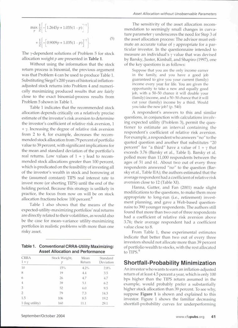
The y-dependent solutions of Problem 5 for stockallocation weight;? are presented in Table 1.

Without using the information that the stockretum process is binomial, the previous argumentwas that Problem 4 can be used to produce Table 1.Substituting Siegel's 200 years of historical inflation-adjusted stock returns into Problem 4 and numeri-cally maximizing produced results that are fairlyclose to the exact binomial-process results fromProblem 5 shown in Table 1.

Table 1 indicates that the recommended stockallocation depends critically on a relatively preciseestimate of the investor's risk aversion to determinethe investor's coefficient of relative risk aversion, 1-I- y. Increasing the degree of relative risk aversionfrom 2 to 4, for example, decreases the recom-mended stock allocation from 79 percent of portfoliovalue to 39 percent, with significant implications forthe mean and standard deviation of the portfolio'sreal returns. Low values of 1 + y lead to recom-mended stock allocations greater than 100 percent,which is predicated on the feasibility of investing allof the investor's wealth in stock and borrowing atthe (assumed constant) TIPS real interest rate toinvest more (or shorting TIPS) until the end of theholding period. Because this strategy is luilikely inpractice, the focus from now on will be on stockallocation fractions below 100 percent.^

Table 1 also shows that the means of theexpected-utility-maximizing portfolios'real returnsare directly related to their volatilities, as would alsobe the case for mean-variance utility-maximizingportfolios in realistic problems with more than onerisky asset.

Table 1

CRRAl + y

10

8

6

4

3

2

1.5

. Conventional CRRA-Utility Maximizing:Asset Allocation and Performance

Stock Weight,

;'

157u

19

26

39

52

79

106

1 (log utility) 160

MeanRetLi rn

4.2'y.,

4.4

4.7

5.1

6.0

7.3

8.5

11.1

StandardDeviation

2.8"''n

3.5

4.7

6.2

y.5

14.3

19.2

29.1

The sensitivity of the asset allocation recom-mendation to seemingly small changes in curva-ture parameter y underscores the need for Step 3 ofthe asset allocation process: The advisor must esti-mate an accurate value of y appropriate for a par-ticular investor. In the questionnaire intended tomeasure an individual's y value that was devisedby Barsky, Juster, Kimball, and Shapiro (1997), oneof the key questions is as follows:

Suppose that you are the only income earnerin the family, and you have a good jobguaranteed to give you your current (family)income every year for life. You are given theopportunity to take a rvew and equally goodjob, with a 50-50 chance it will double your(family) income, and a 50-50 chance that it willcut your (family) income by a third. Wouldyou take the new job? (p. 540)A respondent's answers to this and similar

questions, in conjunction with calculations involv-ing expected utility (Problem 3), permit the ques-tioner to estimate an interval containing therespondent's coefficient of relative risk aversion.For example, a respondent who answers "no" to thequoted question and another that substitutes "20percent" for "a third" have a value of 1 -i- y thatexceeds 3.76 (Barsky et al.. Table 1). Barsky et al.polled more than 11,000 respondents between theages of 51 and 61. About two out of every threerespondents answered "no" to the question (Bar-sky et al.. Table IIA); the authors estimated that theaverage respondent had a coefficient of relati\'e riskaversion close to 12 (Table XI).

Hanna, Gutter, and Fan (2001) made slightmodifications to the questions, to make them moreappropriate to long-run (i.e., retirement) invest-ment planning, and gave a Web-based question-naire to 390 younger respondents. The authors stillfound that more than two out of three respondentshad a coefficient of relative risk aversion above3.76; their average respondent had a coefficientvalue close to 8.

From Table 1, these experimental estimatesindicate that better than two out of every threeinvestors should not allocate more than 39 percentof portfolio wealth to stocks, with the rest allocated

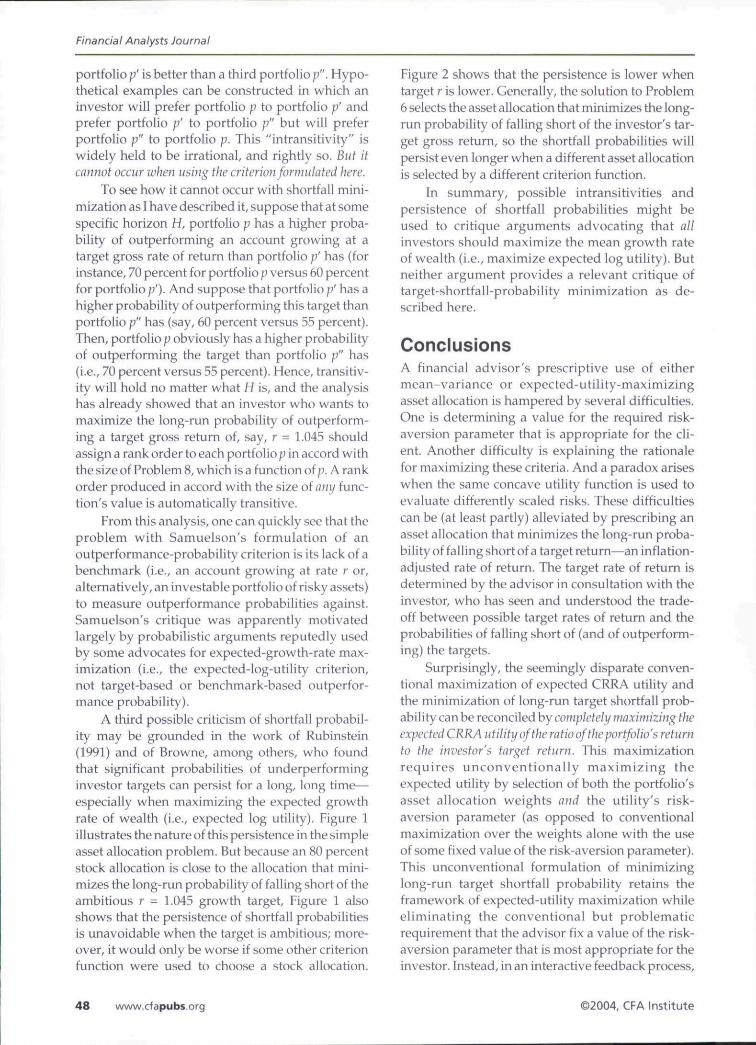
Shortfall-Probability MinimizationAn investor who wants to earn an inflation-adjustedreturn of at least 4.5 percent a year, which is only 100bps higher than the TIPS return assumed in theexample, would probably prefer a substantiallyhigher stock allocation than 39 percent. To see why,suppose Figure 1 is shown and explained to thisiiwestor. Figure 1 shows the familiar decreasingshortfall-probability curves for underperforming

September/October 2004 www.cfapubs.org 41

Financial Analysts Journal

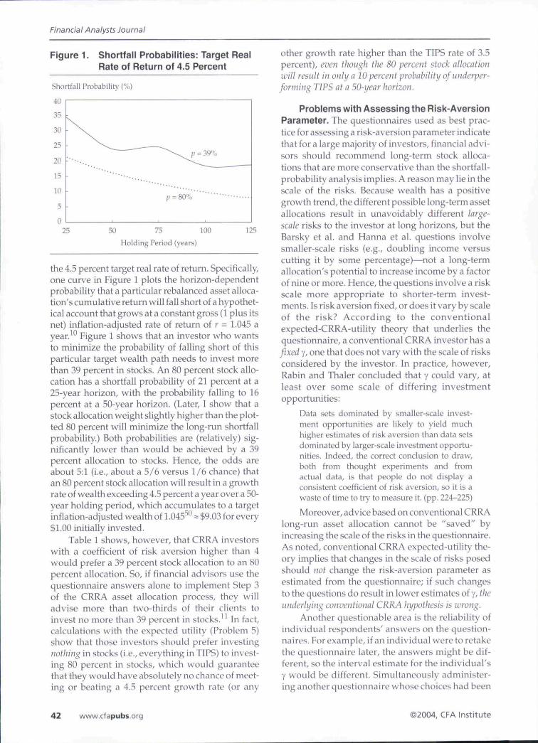
Figure 1. Shortfall Probabilities: Target RealRate of Return of 4.5 Percent

Shortfall Probability (%)

25 50 73 100

Holding Period (years)

the 4.5 percent target real rate of return. Specifically,one curve in Figure 1 plots the horizon-dependentprobability that a particular rebalanced asset alloca-tion's cumulative return will fall short of a hypothet-ical account that grows at a constant gross (1 plus itsnet) inflation-adjusted rate of return of r = 1.045 ayear.^'' Figure 1 shows that an investor who wantsto minimize the probability of falling short of thisparticular target wealth path needs to invest morethan 39 percent in stocks. An 80 percent stock allo-cation has a shortfall probability of 21 percent at a25-year horizon, with the probability falling to 16percent at a 50-year horizon. (Later, I show that astock allocation weight slightly higher than the plot-ted 80 percent will minimize the long-run shortfallprobability.) Both probabilities are (relatively) sig-nificantly lower than would be achieved by a 39percent allocation to stocks. Hence, the odds areabout 5:1 (i.e., about a 5/6 versus 1/6 chance) thatan 80 percent stock allocation will result in a growthrate of wealth exceeding 4.5 percent a year over a 50-year holding period, which accumulates to a targetinflation-adjusted wealth of 1.045̂ *̂ ̂ $9.03 for every$1.00 initially invested.

Table 1 shows, however, that CRRA investorswith a coefficient of risk aversion higher than 4would prefer a 39 percent stock allocation to an 80percent allocation. So, if financial advisors use thequestionnaire answers alone to implement Step 3of the CRRA asset allocation process, they willadvise more than two-thirds of their clients toinvest no more than 39 percent in stocks. In fact,calculations with the expected utility (Problem 5)show that those investors should prefer investingnothing in stocks (i.e., everything in TIPS) to invest-ing 80 percent in stocks, which would guaranteethat they would have absolutely no chance of meet-ing or beating a 4.5 percent growth rate (or any

other growth rate higher than the TIPS rate of 3.5percent), even though the 80 fjercent stock allocationwill result in only a 10 percent probability of underper-forming TIPS at a 50-year horizon.

Problems with Assessing the Risk-AversionParameter. The questionnaires used as best prac-tice for assessing a risk-aversion parameter indicatethat for a large majority of investors, financial advi-sors should recommend long-term stock alloca-tions that are more conservative than the shortfall-probability analysis implies. A reason may lie in thescale of the risks. Because wealth has a positivegrowth trend, the different possible long-term assetallocations result in unavoidably different large-scale risks to the investor at long horizons, but theBarsky et al. and Hanna et al. questions involvesmaller-scale risks (e.g., doubling income versuscutting it by some percentage)—not a long-termallocation's potential to increase income by a factorof nine or more. Hence, the questions involve a riskscale more appropriate to shorter-term invest-ments. Is risk aversion fixed, or does it vary by scaleof the risk? According to the conventionalexpected-CRRA-utility theory that underlies thequestionnaire, a conventional CRRA investor has afixed y, one that does not vary with the scale of risksconsidered by the investor. In practice, however,Rabin and Thaler concluded that y could vary, atleast over some scale of differing investmentopportunities:

Data sets dominated by smaller-scale invest-ment opportunities are likely to yield muchhigher estimates of risk aversion than data setsdominated by larger-scale investment opportu-nities. Indeed, the correct conclusion to draw,both from thought experiments and fromactual data, is that people do not display aconsistent coefficient of risk aversion, so it is awaste of time to try to measure it. (pp. 224-225)

Moreover, advice based on conventional CRRAlong-run asset allocation cannot be "saved" byincreasing the scale of the risks in the questionnaire.As noted, conventional CRRA expected-utility the-ory implies that changes in the scale of risks posedshould not change the risk-aversion parameter asestimated from the questionnaire; if such changesto the questions do result in lower estimates of y, theunderlying conventional CRRA hypothesis is lorong.

Another questionable area is the reliability ofindividual respondents' answers on the question-naires. For example, if an indi\ idual were to retakethe questionnaire later, the answers might be dif-ferent, so the interval estimate for the individual'sy would be different. Simultaneously administer-ing another questionnaire whose choices had been

42 www.cfapubs.org ©2004, CFA Institute

Asset Allocation wittiout Unobservable Parameters

seemingly innocuously altered (e.g., changing theprobabilities or sizes of the gains or losses in a waythat would permit similar interval y estimates tobe made) might also yield a different interval esti-mate for y.

The two survey studies cited here did notaddress this issue, but Yook and Everett (2003)submitted six different qualitative risk-tolerancequestionnaires to 113 part-time MBA students atJohns Hopkins University. The questionnaireswere used by some major brokerages and mutualfunds to provide asset allocation advice for clients.Yook and Everett standardized the risk-toleranceinformation provided by the questionnaires in away that assigned the number 0 to the least risk-tolerant respondent of each questionnaire and thenumber 100 to the most risk tolerant. If differentquestionnaires provided similar information aboutrespondents' risk tolerances, the authors expectedthe 0-100 scores for the respondents to be highlycorrelated. Yet, the 15 possible pairwise compari-sons among the six questionnaires yielded an aver-age pairwise Pearson correlation coefficient of only56 percent. As a result, the authors concluded: '̂̂

the 0.56 average correlation coefficient is muchlower than what we should expect it to be towarrant the use of the questionnaire methodwithout qualm. This low correlation maymanifest the artificiality inherent in the risk-questionnaire design. (Yook and Everett, textabove Table 1)

Moreover, advice based on conventionalexpected-utility asset allocation is not likely to beany less problematic if a different utility function isadopted. Rabin (2000) considered the use of anyconcave utility of wealth to be highly problematic:

The problems with assuming that risk attitudesover modest and large stakes derive from thesame utility-of-wealth function relate to a long-standing debate in economics. Expected-utilitytheory makes a powerful prediction that eco-nomic actors don't see an amalgamation ofindependent gambles as significant insuranceagainst the risk of those gambles; they areeither barely less willing or barely more willingto accept ri5k.s when clumped together thanwhen apart, (p. 1287)

When returns are IID, wealth at the end of horizonH results from the time-averaged sum {the "amal-gamation") of the independent, single-period, loggross portfolio returns (the "independent gam-bles") earned beforehand. The longer the hori-zon, the larger the "stakes."

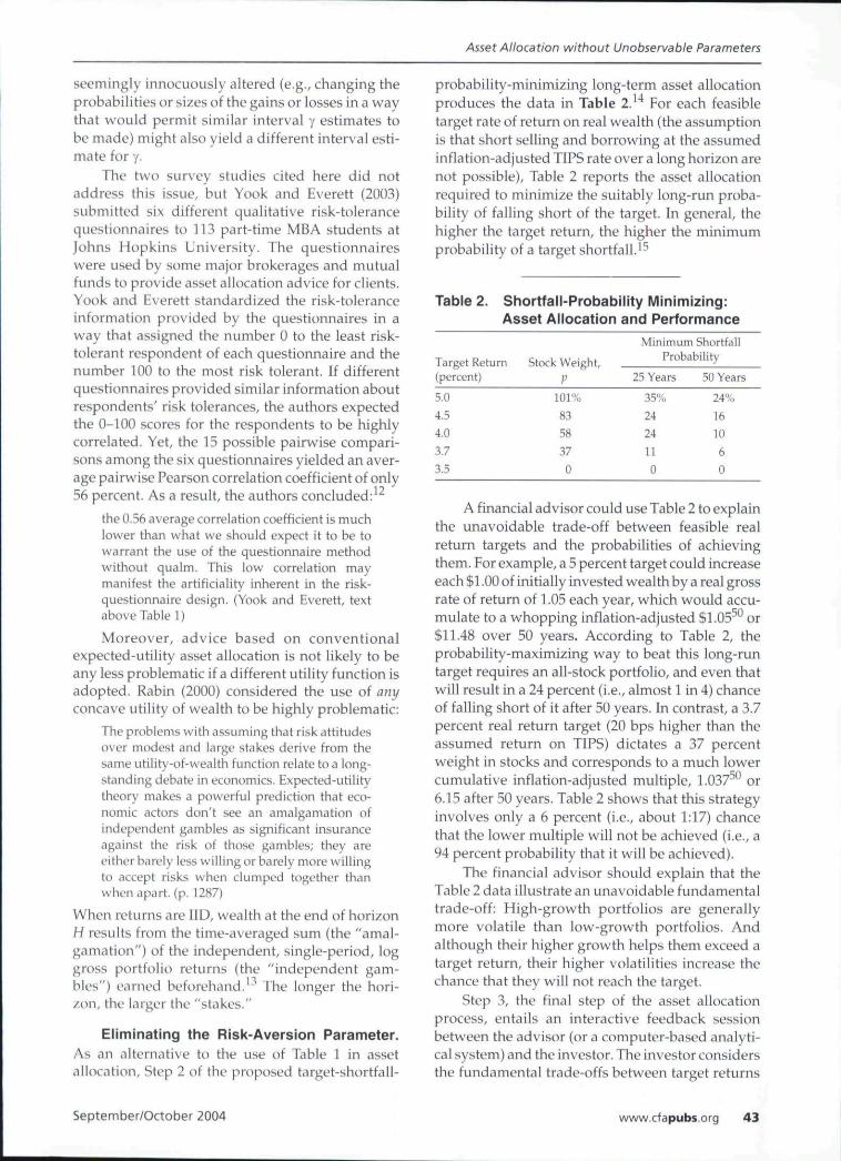
Eliminating the Risk-Aversion Parameter.As an alternative to the use of Table 1 in assetallocation. Step 2 of the proposed target-shortfall-

probability-minimizing long-term asset allocationproduces the data in Table 2.̂ "̂ For each feasibletarget rate of return on real wealth (the assumptionis that short selling and borrowing at the assumedinflation-adjusted TIPS rate over a long horizon arenot possible). Table 2 reports the asset allocationrequired to minimize the suitably long-run proba-bility of falling short of the target. In general, thehigher the target return, the higher the minimumprobability of a target shortfall.^^

Table 2. Shortfaii-Probability Minimizing:Asset Allocation and Performance

Minimum Shortfallfio-h^ Probability

(percent)

5.0

4.5

4.0

3.7

3.5

P101%

83

58

37

0

25 Years

35%

24

24

11

0

50 Years

24%

16

10

6

0

A financial advisor could use Table 2 to explainthe unavoidable trade-off between feasible realreturn targets and the probabilities of achievingthem. For example, a 5 percent target could increaseeach $1.00 of initially invested wealth by a real grossrate of return of 1.05 each year, which would accu-mulate to a whopping inflation-adjusted $1.05̂ *̂ or$11.48 over 50 years. According to Table 2, theprobability-maximizing way to beat this long-runtarget requires an all-stock portfolio, and even thatwill result in a 24 percent (i.e., almost 1 in 4) chanceof falling short of it after 50 years. In contrast, a 3.7percent real return target (20 bps higher than theassumed return on TIPS) dictates a 37 percentweight in stocks and corresponds to a much lowercumulative inflation-adjusted multiple, 1.037̂ "̂ ^ or6.15 after 50 years. Table 2 shows that this strategyinvolves only a 6 percent (i.e., about 1:17) chancethat the lower multiple will not be achieved (i.e., a94 percent probability that it will be achieved).

The financial advisor should explain that theTable 2 data illustrate an unavoidable fundamentaltrade-off: High-growth portfolios are generallymore volatile than low-growth portfolios. Andalthough their higher growth helps them exceed atarget return, their higher volatilities increase thechance that they will not reach the target.

Step 3, the final step of the asset allocationprocess, entails an interactive feedback sessionbetween the advisor (or a computer-based analyti-cal system) and the investor. The investor considersthe fundamental trade-offs between target retums

September/October 2004 www.cfapubs.org 43

Financial Analysts Journal

(or the investor's equivalent target wealth levels)and the probabilities of falling short of them (orcomplementary probabilities of exceeding them) atvarious horizons. Based on this assessment, theinvestor who initially wanted a high target returnmight revise the return expectations downwardbecause a lower target is associated with a lowerprobability of shortfall. If the investor must fund afixed inflation-adjusted liability that is expected onsome future date, the advisor can explain that theinvestor should also expect to invest a higher frac-tion of income to compensate for the lower targetreturn. This trade-off might prompt the investor toagain reconsider other feasible targets, savingsfractions, and so on, until a satisfactory return tar-get is established. Finally, the investor is advised toselect the optimal asset allocation associated withthe satisfactory return target.

Don't put the cart before the horse. An advisorwho adopts a conventional y-dependent mean-variance or other expected-utility criterion in StepI of the asset allocation process might argue thatexplanations of the trade-offs shown in Table 2and/or the mean-variance statistics in Table 1 canbe used to help the financial advisor measure aninvestor's y. For example, an investor who receivesthe explanation of Table 2 might decide to adopt atarget real rate of return of 4.0 percent and thusinvest 58 percent in stocks. Table 1 indicates that aninvestor who wishes to maximize expected CRRAutility and who has a (supposedly) constant coeffi-cient of risk aversion that is slightly less than 3would also choose to allocate 58 percent to stocks.Hence, the financial advisor might be tempted toinfer that 3 is "the" value of y that can reliably beused to recommend an asset allocation for thisinvestor. Similarly, a financial advisor who adoptsa mean-variance utility might be tempted topresent the trade-off information in Table 2 to aninvestor to "reverse engineer" a value for theappropriate mean-variance utility's required risk-aversion parameter.

In realistic situations, however (that is, whenmultiple risky asset classes are available), an advi-sor's attempts to use shortfall probability as auxil-iary information in Step 3 may lead to results thatare internally inconsistent with the expected-utilityor mean-variance criterion adopted in Step 1. Tosee why, suppose there is one other asset class inaddition to domestic stocks and TIPS—for example,an international stock index fund. To elicit a valuefor the investor's target real rate of return, a finan-cial advisor could expand Table 2 to include inter-national stock and use the table to explain the assetallocation trade-offs. For illustration, assume thisexplanation has been made and that the corre-

sponding recommendation to minin^ize targetshortfall probability is to invest 50 percent indomestic stocks, 20 percent in intemational stocks,and the rest (30 percent) in TIPS. The required three-asset allocation analogous to Table 1 will probablynot show even a single value of 1 H- y that would leadby conventional cxpected-CRRA-utility maximizationto these three specific percentages.

The attempt to reverse engineer a y value in thisexample would fail, but this failure should not bemourned, because it prevents the financial advisorfrom placing the cart (Step 3) before the horse {Step1). The recommended asset allocation must be inter-nally consistent with the optimization criterionused to produce that allocation. Investors may wellfind shortfall (or outperformance) probabilities tobe useful and informative because they rationallywant to minimize (maximize) the target shortfall(outperformance) probabilities instead of beingforced to use the expected-utility or mean-variancecriterion that the advisor adopted in Step 1.

For example, that mean-variance investorscare only about the mean and variance of theirfuture wealth and that they maximize the criterion|i - yo- are axiomatic. A mathematical theoreticalimplication of this is that the investor, to select aspecific combination of mean and variance andspecific asset allocation that will generate it, needsto know only the mean-variance wealth trade-offson the efficient frontier permitted by the invest-ment opportunity set. For that investor to also needto know various target shortfall or outperformancestatistics is inconsistent, unless those statistics pro-vide absolutely no information other than what isalready provided by the asset means and variances.

Yet, even legendary mean-variance-analysisadvocate William Sharpe recommends the use ofthe Financial Engines website, which contains thefollowing example of how an investor can use itsprobabilistic assessments:

For example, a person with a 40 percentchance of achieving an income goal of $50,000may find that tolerable if they have a 95percent chance of achieving an income of$40,000 (in other words, their long-term down-side income is $40,000).̂ ^

Unless portfolio returns are either normally dis-tributed or from some other two-moment familyof distributions, the quote provides more informa-tion than can be obtained from the mean and vari-ance associated with the return distribution of theasset allocation being analyzed. Thus, although thecriterion inherent in the quote does not exactlystate the shortfall (outperformance) probabilitycriterion developed in this article, it certainly issimilarly motivated.

44 www.cfapubs.org ©2004, CFA Institute

Asset Allocation without Unobservable Parameters

Reconciliation of MethodsThe previous section illustrated how a financialadvisor might use Table 2, in conjunction withinput from an investor client, to recommend aspecific long-run shortfall-probability-minimizingasset allocation. How were those target return-dependent asset allocations found? A theoreticalextension of the results in Stutzer (2000, 2003)shows that the optimal long-term asset allocationscan be found by solving the following problem:

max max £p y

(6)

Problem 6 differs from the conventional use ofCRRA utility (Problem 3) by the presence of thetarget (gross) retum per year, r, as well as the innermaximization over y prior to maximizing overstock weight p. For the r = I.(M5 gross return targetused to produce Figure 1, Problem 6 is the follow-ing simple modification of Problem 5:

(7)

1 1max max - •{ -

P 7 2 1.045

0.9009p +1.035(1-1.045

Numerically solving Problem 7 in a spread-sheet yields p = 82.7 percent, as indicated in Table2 (to the nearest percentage), which is close to the80 percent allocation used for illustrative purposesin Figure 1. The optimized value of y associatedwith the optimal p = 82.7 percent is approximately0.9, but this should not be taken to imply that theinvestor with a 4.5 percent target return has a con-stant coefficient of relative risk aversion of 1.9.Through the inner maximization over y in Problem7, the investor uses a different (inner-maximizing)value of y to evaluate each specific p. So, althoughthe 4.5 percent target investor does use a value of y== 0.9 when evaluating the expected utility of a '̂ -82.7 percent allocation, this same investor uses aninner-maximized value of y = 1.3 when evaluatingthe alternative (suboptimal) p = 39 percent alloca-tion used to prod uce Figure 1. Simply put, an inves-tor ranks the desirability of the various assetallocations by using the following function of p:

(8)max E -\

•I I I rL rnax 1 i -

Y 2 1 1.045

1.035(1-;?)1.045

The other long-term allocations in Table 2 wereproduced by successively substituting each alter-native target gross return for the number 1.045 in

Problem 7 and then solving it by using the maxi-mizing routine in a spreadsheet.

In summary, conventional expected-CRRA-utility maximization and long-run target-shortfall-probability minimization can be reconciled byeliminating the conventional assumption thatexpected utility should be only partially maxi-mized (i.e., maximized only over the possible assetallocations), rather than totally maximized overboth the asset allocations and the positive values ofy. This unconventional use of expected-utility the-ory (conventional expected-utility maximizationholds the risk-aversion pa rameter fixed) is an appli-cation of theoretical results proven in Stutzer (2000,2003). An analyst who (mis)specifies a conven-tional power utility function for a long-run investorwho is seeking to minimize a target shortfall prob-ability should find that the utility function's risk-aversion "parameter" is not a fixed constant but,instead, a variable that depends on the investor'starget and the investment opportunity set.

Modifications for RealisticSituationsSome modifications of the computations are recom-mended for the realistic applications faced by prac-ticing advisors. First, the numerical example dealtwith only two assets, one of which was assumed toresult in a constant real return (i.e., a constant realinterest rate). In practice, advisors will consider adiverse group of assets, none of which earn a con-stant real rate of return. But despite the diversity ofavailable asset classes, advisors should strive toavoid recommendations involving a large numberof asset classes. Because of the inherent uncertaintyin the use of historical return series, an analystconsidering a large number of asset classes will beforced to make overly specific and possibly smallpercentage recommendations (e.g., invest 3 percentin South Korean stocks, 2 percent in Colorado realestate investment trusts, etc.). Such specifics con-vey an unrealistic degree of precision.

Second, the example investor's target was apurely hypothetical account growing at a fixed realrate of return. The advisor should make sure theinvestor understands that such an account is not aninvestable benchmark and, therefore, cannot bematched with certainty. In practice, however,investors might designate an investable bench-mark (e.g., an S&P 500 Index mutual fund orexchange-traded fund), which can be matched byinvesting 100 percent in it. In either case, the advi-sor needs to find the asset allocation with the bestchance of actually beating the noninvestable targetor investable benchmark.

September/October 2004 www.cfapubs.org 45

Financial Analysts Journal

When the assets' returns are jointly IID, onlysimple modifications to Problem 6 are needed.With the nth asset's real return in historical periodt denoted by R,,,, an N-asset portfolio's real returnwith constantly rebalanced asset (value-weighted)proportions ZV],..., zv^--[ is denoted

N-l

(1=1

(9)

If an investable benchmark is designated, theadvisor denotes its return in historical period t byR̂ f. After entering the historical data in a spread-sheet or computer program, the advisor simplyuses the numerical maximizer to solve the follow-ing simple generalization of Problem 4:

max max (10)

That is, the advisor substitutes the designatedbenchmark return, R;,, for r in Problem 6 and thenuses the historical average to estimate theexpected value in that formula. As in using anyportfolio optimizer, the advisor can constrain theweights in Problem 10 to be nonnegative if shortselling is precluded. A problem is that numericalsolutions may be extreme when highly correlatedassets are present. This may also happen whenmean-variance-optimizing software is used. Thisproblem provides another reason to restrict atten-tion to a limited number of broad, disparate assetclasses whose returns are not highly correlatedwith one another.

Also, to ensure that a numerical solution toProblem 10 does indeed exist, a rebalanced portfo-lio of the assets needs to be available that, whengiven enough time, can beat the investor's target ordesignated benchmark portfolio. Thus, the rebal-anced portfolio's expected log gross return shouldexceed the target or benchmark's expected logreturn (Stutzer 2003). In practice, with historicalreturn data subject to these provisos, a numericalsolution to Problem 10 has been easily obtained byusing a spreadsheet optimizer. A valid solutionfinds a positive value for y.

The assumption that returns are IID may notapproximate the actual situation well enough,however, for Problem 10 to be applied with confi-dence that the recommendations will yield the bestallocation. For example, Siegel's (pp. 38-39) exam-ination of stocks' historical real returns led him toassume that future stock returns would be meanreverting rather than IID. He thus concluded thatadvisors should recommend considerably higherstock allocations than would otherwise be the case.Fortunately, Problem 10 can be modified to accom-

modate non-IID returns (Foster and Stutzer 2002).The required formula still involves maximizingover all possible values of a risk-aversion parame-ter, but it is more complicated than Problem 10.Instead, advisors can estimate asset allocation-dependent shortfall-probability curves (like thosein Figure 1) directly. To do so, one first fixes assetallocation weights (i.e., a specific rebalanced port-folio); then, one applies a straightforward tech-nique of bootstrapping with moving blocks (e.g.,see Hansson and Persson 2000) to simulate numer-ous future return scenarios for the portfolio and thedesignated benchmark. From the scenarios, onetabulates the fraction of times the portfolio's cumu-lative return at horizon H falls short of the desig-nated benchmark 's cumulat ive return. Thisfraction is the estimate of the portfolio's shortfallprobability at horizon H. By repeating this proce-dure for other portfolios (i.e., other asset allocationweights), a computer program searches for the spe-cific asset allocation weights with the lowest short-fall probability at H. Long-run investors shouldadopt an asset allocation that minimizes the short-fall probabilities for suitably large values of H.

Reexamining the ArgumentsGiven the behavioral evidence favoring targetshortfall criteria and the implementational advan-tages of shortfall-probability minimization, a reex-amination of the typical arguments made in favor ofthe conventional use of expected utility and againstthe use of shortfall probability will be useful.

The normative case for conventional use ofexpected utility is grounded in the Von Neumann-Morgenstern (1980) axioms for decision making inrisky situations. Von Neumarm and Morgenstemstarted from the postulate that a decision maker isable to rank-order the desirability (i.e., from mostdesirable to least desirable) of different probabilitydistributions of wealth ("wealth lotteries") result-ing from the various feasible decisions. They posedseemingly sensible axioms that decision makersmight adhere to when composing this rank order.They proved that a decision maker acting in accordwith those axioms acts as if he or she had adoptedsome utility function and had then rank-ordered theprobability distributions in accord with the size oftheir respective expected utilities. Hence, the deci-sion maker's top-ranked decision should be the onethat leads to the distribution of wealth with thehighest expected utility.

The problem with this and other axiomatic"rationalizations" for expected-utility maximiza-tion is that axioms that appear to be reasonable onfirst examination do not always remain so after

46 www.cfapubs.org ©2004, CFA Institute

Asset Allocation wittiout Unobservable Parameters

closer examination. For example, much reconsider-ation has been given to Von Neumann and Morgen-stem's crucial "independence axiom," withoutwhich there can be no conventional expected utility.Machina (1987) summarized the evidence showingthat most individuals' choices violate this axiom andhence cannot be consistent with expected-utilitymaximization. Moreover, Rabin and Rabin and Tha-ler pointed out the paradoxical behavior towarddifferently scaled risks by anyone who does maxi-mize an expected concave utility—such as Problem 3with Y > 0, as in the example 1 discussed.

In light of these negative findings aboutexpected-utility maximization, the case against theuse of shortfall probabilities is not compelling.Much of it appears to be associated with earlyarguments made by Samuelson (1963).̂ ^ The fol-lowing reexamination of Samuelson's argumentsagainst shortfall probability will show that theyeither are overstated or do not apply to the criterionof minimizing target shortfall probability.

Samuelson correctly noted that in repeatedbetting situations analogous to long-run asset allo-cation, even though the probability of falling shortof some wealth target (which could be merewealth preservation) is low, "the improbable losswill be very great indeed if it does occur" (p. 110).Although technically correct, this statement mightlead readers to believe that minimizing the short-fall probability will induce excessively risky behav-ior (presumably, by failing to adequately weighthe prospect of great but improbable shortfalls).But Samuelson also noted the obvious point thatthe probability of outperformance is the comple-ment of the shortfall probability, so minimizingshortfall probability is the same as maximizingoutperformance probability. Hence, readersmight just as well believe that a criterion of target-outperformance-probability maximization isflawed because the improbable gain will be verygreat indeed if it does occur, inducing excessivelyconserzmtive behavior!

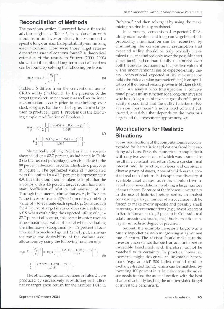
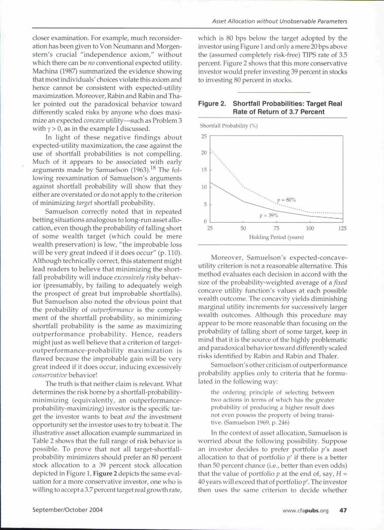
The truth is that neither claim is relevant. Whatdetermines the risk borne by a shortfall-probability-minimizing (equivalently, an outperformance-probability-maximizing) investor is the specific tar-get the investor wants to beat and the investmentopportunity set the investor uses to try to beat it. Theillustrative asset allocation example summarized inTable 2 shows that the full range of risk behavior ispossible. To prove that not all target-shortfall-probability minimizers should prefer an 80 percentstock allocation to a 39 percent stock allocationdepicted in Figure 1, Figure 2 depicts the same eval-uation for a more conservative investor, one who iswilling to accept a 3.7 percent target real growth rate.

which is 80 bps below the target adopted by theinvestor using Figure 1 and only a mere 20 bps abovethe (assumed completely risk-free) TIPS rate of 3.5percent. Figure 2 shows that this more conservativeinvestor would prefer investing 39 percent in stocksto investing 80 percent in stocks.

Figure 2. Shortfall Probabilities: Target RealRate of Return of 3.7 Percent

Shortfall Probability (%)

20

15

10

5

n

•

p - 39%

J - 80%

25 50 75 100Holding Period (years)

125

Moreover, Samuelson's expected-concave-utility criterion is not a reasonable alternative. Thismethod evaluates each decision in accord with thesize of the probability-weighted average of a. fixedconcave utility function's values at each possiblewealth outcome. The concavity yields diminishingmarginal utility increments for successively largerwealth outcomes. Although this procedure mayappear to be more reasonable than focusing on theprobability of falling short of some target, keep inmind that it is the source of the highly problematicand paradoxical behavior toward differently scaledrisks identified by Rabin and Rabin and Thaler.

Samuelson's other criticism of outperformanceprobability applies only to criteria that he formu-lated in the following way:

the ordering principle of selecting betweentwo actions in terms of which has the greaterprobability of producing a higher result doesnot even possess the property of being transi-tive. (Samuelson 1969, p. 246)

In the context of asset allocation, Samuelson isworried about the following possibility. Supposean investor decides to prefer portfolio p's assetallocation to that of portfolio p' if there is a betterthan 50 percent chance (i.e., better than even odds)that the value of portfolio p at the end of, say, H -40 years will exceed that of portfolio p'. The investorthen uses the same criterion to decide whether

September/October 2004 www.cfapubs.org 47

Financial Analysts Journal

portfolio p' is better than a third portfolio p". Hypo-thetical examples can be constructed in which aninvestor will prefer portfolio p to portfolio p' andprefer portfolio p' to portfolio p" but will preferportfolio p" to portfolio p. This "intransitivity" iswidely held to be irrational, and rightly so. But itcannot occur zvhen using the criterion formulated here.

To see how it cannot occur with shortfall mini-mization as I have described it, suppose that at somespecific horizon H, portfolio p has a higher proba-bility of outperforming an account growing at atarget gross rate of return than portfolio p' has (forinstance, 70 percent for portfolio p versus 60 percentfor portfolio p'). And suppose that portfolio p' has ahigher probability of outperforming this target thanportfolio p" has (say, 60 percent versus 55 percent).Then, portfolio p obviously has a higher probabilityof outperforming the target than portfolio p" has(i.e., 70 percent versus 55 percent). Hence, transitiv-ity will hold no matter what H is, and the analysishas already showed that an investor who wants tomaximize the long-run probability of outperform-ing a target gross return of, say, r - 1.045 shouldassign a rank order to each portfolio p in accord withthe size of Problem 8, which is a function of p. A rankorder produced in accord with the size of any func-tion's value is automatically transitive.

From this analysis, one can quickly see that theproblem with Samuelson's formulation of anoutperformance-probability criterion is its lack of abenchmark (i.e., an account growing at rate r or,alternatively, an investable portfolio of risky assets)to measure outperformanee probabilities against.Samuelson's critique was apparently motivatedlargely by probabilistic arguments reputedly usedby some advocates for expected-growth-rate max-imization (i.e., the expected-log-utility criterion,not target-based or benchmark-based outperfor-mance probability).

A third possible criticism of shortfall probabil-ity may be grounded in the work of Rubinstein(1991) and of Browne, among others, who foundthat significant probabilities of underperforminginvestor targets can persist for a long, long t ime-especially when maximizing the expected growthrate of wealth (i.e., expected log utility). Figure 1illustrates the nature of this persistence in the simpleasset allocation problem. But because an 80 percentstock allocation is close to the allocation that mini-mizes the long-run probability of falling short of theambitious r = 1.045 growth target. Figure 1 alsoshows that the persistence of shortfall probabilitiesis unavoidable when the target is ambitious; more-over, it would only be worse if some other criterionfunction were used to choose a stock allocation.

Figure 2 shows that the persistence is lower whentarget r is lower. Generally, the solution to Problem6 selects the asset allocation that minimizes the long-run probability of falling short of the investor's tar-get gross return, so the shortfall probabilities willpersist even longer when a different asset allocationis selected by a different criterion function.

In summary, possible intransitivities andpersistence of shortfall probabilities might beused to critique arguments advocating that allinvestors should maximize the mean growth rateof wealth (i.e., maximize expected log utility). Butneither argument provides a relevant critique oftarget-shortfall-probability minimization as de-scribed here.

ConclusionsA financial advisor's prescriptive use of eithermean-variance or expected-utility-maximizingasset allocation is hampered by several difficulties.One is determining a value for the required risk-aversion parameter that is appropriate for the cli-ent. Another difficulty is explaining the rationalefor maximizing these criteria. And a paradox ariseswhen the same concave utility function is used toevaluate differently scaled risks. These difficultiescan be (at least partly) alleviated by prescribing anasset allocation that minimizes the long-run proba-bility of falling short of a target return—an inflation-adjusted rate of return. The target rate of return isdetermined by the advisor in consultation with theinvestor, who has seen and understood the trade-off between possible target rates of return and theprobabilities of falling short of (and of outperform-ing) the targets.

Surprisingly, the seemingly disparate conven-tional maximization of expected CRRA utility andthe minimization of long-run target shortfall prob-ability can be reconciled by completely maximizing theexpected CRRA utility of the ratio of the portfolio's returnto the investor's target return. This maximizationrequires unconventionally maximizing theexpected utility by selection of both the portfolio'sasset allocation weights a?id the utility's risk-aversion parameter (as opposed to conventionalmaximization over the weights alone with the useof some fixed value of the risk-aversion parameter).This unconventional formulation of minimizinglong-run target shortfall probability retains theframework of expected-utility maximization whileeliminating the conventional but problematicrequirement that the advisor fix a value of the risk-aversion parameter that is most appropriate for theinvestor. Instead, in an interactive feedback process.

48 www. cf apu bs.org ©2004, CFA Institute

Asset Allocation without Unobservable Parameters

the advisor and the investor mutually determine themost appropriate target rate of return or investablebenchmark the investor wants to beat.

Criticisms of the use of shortfall probabilityare either overstated or not applicable to target-shortfall-minimization (target-outperformance-maximization) probability as described here. The-orists who believe that this criterion is inferior torisk-aversion-parameter-dependent expected util-

ity need to reevaluate that position in light of theimplementation and the risk-scaling problemshighlighted in this article.

The author thanks Tom Rietz for information aboutquestionnaire-based risk-aversion estimates. This workbenefited from a large nnmber of questions and com-ments offered by participants in numerous academic andpractitioner forums around the world.

Notes1. Because I focus solely on the asset allocation advice for long-

term investors, I do not address the controversial subject oftime diversification.

2. Moreover, any future critiijue.s of this criterion must beconsidered in lij;ht of the new and surprisingly devastatingcriticisms in Rabin (2000) and Rabin and Tlialer that applyto all conventional expected-concave-utility-of-wealth crite-ria favored by Samuelson {1963, 1969).

3. Mossin (1968) used a more complicated dynamic program-ming method to study this problem. A later influentialpaper by Samuelson (1969) used a different criterionfunction—the time-additive sum of single-period CRRAutilities of consumption during the holdinj:^ period. Mossin'send-of-holding-period utility of wealth did not permitwithdrawals for consumption until the end of the holdingperiod. Hence, the derivations in Samuelson (1969) do notapply to the problem studied in this paper, although theydo lead to similar results.

4. A simple proof follows. Set WQ = 1 in Equation 2,which produces the equivalent criterion function of-E [ I I .^,,,(1 - When returns are independentlydistributed, we can move the expectation operator inside

the product to yield - £{R )i

immediately seethat the portfolio weights that maximize this function willbe the weights that minimize FT" E(R~-)- Moreover,because the logarithmic function is monotonically increas-ing, the same weight vectors will also minimizetog FT" E(R ,7 , )^y^ iogE(R-\). Because this prob-lem is additively separable, the first-order necessarycondition for any particular p, will not include any nf theother ^,'s. As a result, p, can be found simply byminimizing E( R~ ,̂). If we make use of the assumption thatportfolio retums are independently distributed across theH equal-length periods, we can remove the subscript ffrom p, in this problem, producing E{R~/). MultiplyingE(Rj',')by -1 converts it into the one-period maximizationin the article (Problem 3).

5. In practice, rebalancing may also be a useful strategy formaximizing other criterion functitms, even when a moreelaborate dynamic strategy could, in theory, do better (e.g.,when portfolio returns are not ilD). Buetow, Sellers, Trotter,Hunt, and Whipple (2002) documented some of the generalbenefits of rebalancing.

6. Later, I describe how the analysis should be modified toaddress realistic applications with multiple assets, morerealistic return processes, and a situation in which no assetearns a constant real rate of return.

7. Matching the average real stock return requires the solutionof one equation in the two unknowns, u and d; matching the

standard deviation requires the solution of another equa-tion in the two unknowns. The assumed values of ii and dare the only ones satisfying both equations. They arereported to only four decimal places in the text, but moreaccurate floating point values were used in the computa-tions. Because of this discrepancy, readers may be unableto exactly duplicate the calculations that yielded the tableshere hut should get close enough to determine whether theyare doing them correctly.

8. Restricting investors to using stocks and non-inflation-indexL'ii bonds, Siegel derived a mean-variance-efficientstock allocation of 115 percent for an investor with a 30-yearhorizon and what he described as "moderate risk tolerance"(p. 38). This high percentage iiccurred because his 20()-yearseries of inflation-adjusted stock returns has some of theproperties typical of series generated from a mean-revertingprocess rather than an IID process. As a result, the 30-yearcumulative real returns presented in his series have lowervolatility than would occur if retums were ilDand were thusmore favorably appraised by his mean-variance criterionthan TiD returns would be. When the possibility of allocatingassets to TIPS (earning an assumed real rate of 3.5 percent ayear) was added, the mean-variance-efficient "tangency"portfolio (of only the stocks and non-inflation-indexedbonds) for an investor with a horizon of 10 years still allo-cated 185 percent to stocks; hence, it was 85 percent short inbonds. A mean-variance utility-maximizing investor's risk-aversion parameter would then determine only the relativesplit of wealth between that portfolio and TII^. Siegel thusconcluded, "Stocks should constitute the overwhelmingproportion of ail long-term financial portfolios" (p. 361).Because my purpose was to use the simplest possible assetallocation problem to illustrate the crucial implementatiunaldifferences between conventional mean-variance andexpected-utility criteria and the target-shortfall-probabilitycriterion, 1 did not use the controversial hypothesis that realstock returns are in fact (rather than simply historicallyappearing to be) generated by a mean-reverting process. Butlater, I do describe the modifications required to adapt thecomputations to incorporate mean reversion and/or otherapparent deviations trom the example's IID assumption.

9. Of course, implicit in Table 1 is an assumption that theinvestoris concerned only about inflation-adjusted investedwealth at one point in time (i.e., H years in the future). Siegelmade this assumption, as have many others in applicationsof portfolio choice theory. Because Siegel's focus was (andmy focus is) on asset allocation advice for long-term inves-tors, horizon H might be thought of as the number of yearsuntil the investor will retire or die. In the case of retirementperhaps (and surely in the case of death), the advice shouldnot be too dependent on knowing the particular value of H!Fortunately, advice based on Table 1 does not depend at allon H, although such need not be the case when retums arenon-llD.

September/October 2004 www. cf a pubs, o rg 49

Financial Analysts Journal

10. For each stock weight;', let Rp denote the portfolio's gross(1 plusitsnet)retumwhenthestockgoesupand Rj, denotethe portfolio's gross return when the stock goes down. Fora horizon length T, shortfall occurs when there are x orfewer up moves—that is, when .YR!'(r-.v)R|'< 1.045 .Hence, the probability of shortfall is computed by evaluat-ing the cumulative binomial distribution (with probabilityof an up move equal to 1 /2) at the highest integer x satisfy-ing this inequality. This caiculation can be easily accom-plished in a spreadsheet.

11. Technically, some of these individuals might haverevealed a coefficient of risk a version between 3.76 and 4.00by this single answer, although the questionnaire providesno way to tell.

12. I thank Michele Gambera of Morningstar for providing thisreference. Although the six questionnaires did not attemptto estimate an investor's risk tolerance in the quantitativeway described by Barsky et al. and Hanna et al., the resultsindicate that an analogous study of reliability is warranted,one in which different questionnaires pose quantitativelydifferent wealth lotteries. {^H "\

13. Thatis, Wf,= lYu]-[« R,,,.W,A^--''''^''''"'''J".

14. The next section describes how this table was produced andhow it could he produced in more realistic problems.

15. The relationship between target return and probability inTable 2 is only weakly (rather than strictly) monotonic

because of the discrete, binomial distribution process usedto model the sttKk return. The relationship would be strictlymonotonic had an absolutely continuous (e.g., lognormal)distribution been assumed in the calculations, and onewould obtain a strictly increasing relationship between thetarget return and the (minimized) probability of fallingshort of it at any horizon H.

16. The Financial Engines website (www.financialenglnes.com) describes Sharpe as "Founder Bill Sharpe" anddescribes his role as follows: "One of the fathers of ModernPortfolio Theory, Nobel laureate Dr. Sharpe has helpedsome of the nation's largest pension fund managers investbillions of dollars of retirement money. When he realizedthat he could offer this help to individuals through anadvice technology platform, he started Financial Engines.Financial Engines comhines Dr. Sharpe's pioneering invest-ment methodology with scalable technology to provide allinvestors with cost-effective, expert advice."

17. This sentence was found in the "Common Questions" sec-tion of www.financialengines.com as part of the answer tothe question: "What is a good Forecast?" In the quote, the"Forecast" is the 40 percent probability of outperformingthe investor's $50,000 target (i.e., "income goal").

18. Arguments in Samuelson (1963) were repeated in numerouslater articles; see Samuelson 1969; Merton and Samuelson1974; Samuelson 1979).

ReferencesBarsky, R.B., F.T. Juster, M.S. Kimball, and M.D. Shapiro. 1997."Preference Parameters and Behavioral Heterogeneity: AnExperimental Approach in the Health and Retirement Study."Quarterly journal of Economics, vol. 112, no. 2 (May):537-579.

Browne, Sid. 1999. "The Risk and Rewards of MinimizingShortfall Probability." journal of Portfolio Management, vol. 25,no. 4 (Summer):76-85.

Buetow, Gerald W., Ronald Sellers, Donald Trotter, Elaine Hunt,and Willie A. Whipple. 2002. "The Benefits of Rebalancing."journal of Portfolio Management, vol. 28, no. 2 (Winter):23-32.

Foster, F. Douglas, and Michael Stutzer. 2002. "Performanceand Risk Aversion of Funds with Benchmarks: A LargeDeviations Approach." Working paper. University of ColoradoFinance Department.

Hakansson, Nils H., and William T. Ziemba. 1995. "CapitalGrowth Theory." In Handbooks in Operations Research andManagement Science: Finance, vol. 9. Edited by Robert A. Jarrow,Vojislav Maksimovic, and William T. Ziemha. Amsterdam:North Holland.

Harma, Sherman D., Michael S. Gutter, and Jessie X. Fan. 2001."A Measure of Risk Tolerance Based on Economic Theory."Financial Counseling and Planning, vol. 12, no. 2:1-8.

Hansson, Bjorn, and Mattias Persson. 2000. "TimeDiversification and Estimation Risk." Financial Analysts journal,vol. 56, no. 5 (September/October):55-62.

KroU, Yoram, Haim Levy, and Harry Markowitz. 1984. "Mean-Variance versus Direct Utility Maximization." journal of Finance,vol.39, no. l(March):47-61.

Leibowitz, Martin, and R. Henriksson. 1989. "TortfolioOptimization with Shortfall Constraints: A Confidence-LimitApproach to Managing Downside I^sk." Financial AnalystsJournal, vol. 45, no. 2 (March/Aprii):34r-41.

Leibowitz, Martin, and Terence Langetieg. 1989. "Shortfall Riskand the Asset Allocation Decision: A Simulation Analysis ofStock and Bond ProMes." joiirnalof Portfolio Management,vol. 16,no. 1 (Fall):61-68.

Leibowitz, Martin, Lawrence Bader, and Stanley Kogelman.1996. Return Targets and Shortfall Risks. Chicago, IL: Irwin.

Machina, Mark J. 1987. "Choice under Uncertainty: ProblemsSolved and Unsolved." Eco)wmic Perspectives, vol. 1, no. 1(Summer):121-154.

Merton, Robert, and Paul Samuelson. 1974. "Fallacy of the Log-Normal Approximation to Optimal Portfolio Decision-Makingover Many Periods." journal of Financial Fconomics, vol. 1, no. 1(May):67-94.

Milevsky, Moshe. 1999. "Time Diversification: Safety First andRisk." Rroiem of Quantitative Finance and Accounting, vol. 12, no. 3(May):271-281.

Mossin, Jan. 1968. "Optimal Multiperiod Portfolio Policies."journal of Business, vol. 41, no. 2 (Apri!):215-229.

Olsen, Robert A. 1997. "Investment Risk: The Experts'Perspective." Financial Analysts journal, vol. 53, no. 2 (March/April):62~66.

Olsen, Robert A., and Muhammad Khaki. 1998. "Risk,Rationality, and Time Diversification." Financial Analystsjournal, vol. 54, no. 5 (September/October):58-63.

Rabin, Matthew. 2000. "Risk Aversion and Expected-UtilityTheory: A Calibration Theorem." Econometrica, vol. 68, no. 5(September):1281-92.

Rabin, Matthew, and Richard Thaler. 2001. "Anomalies: RiskAversion." journal of Economic Perspectives, vol. 15, no. 1(Winter):219-232.

Reichenstein, William. 1986. "When Stock Is Less Risky ThanTreasury Bills." Financial Analysts journal, vol. 42, no. 6(November/December ):71-75.

50 www.cfapubs.org ©2004, CFA Institute

Asset Allocation without Unobservable Parameters

Rubinstein, Mark. 199L "Conhnuously Rebalanced InvestmentStrategies." journal of Portfolio Maiuigcmcnt, vol. 18, no. 1(Fall):78-81.

Samuelson, Paul A. 1963. "Risk and Uncertainty: A Fallacy ofLarge Numbers." Scicntia, vol. 98, no. 4 (April/May):lC8-113.

. 1969. "Lifetime Portfolio Selection by DynamicProgramming." Review of Economics and Statistics, vol. 51, no. 3(August):239-246.

. 1979. "Why We Should Not Make Mean Log of WealthBig Though Years to Act Are Long." journal of Banking andFinance, vol. 3, no. 4:305-307.

Siegel, Jeremy J. 2002. Stocks for the Long Run. 3rded. New York:McGraw-Hill.

Stutzer, Michael. 2000. "A Portfolio Performance Index."Financial Analysts journal, vol. 56, no. 3 (May/June):52-61.

. 2003. "Portfolio Choice with Endogenous Utility: ALarge Deviations Approach." jouriinl of E-coiiometrics, vol. 116,nos. 1-2 (September-October):36.S-386.

Thorp, Edward O. 1975. "Portfolio Choice and the KellyCriterion." In Stochastic Optimization Models in Finance. Editedby W.T. Ziemba and R.G. Vickson. New York: Academic Press.

Von Neumann, John, and Oskar Morgenstem. J980. Theory ofGames and Economic Behavior. (Eirst published in 1944.)Princeton, NJ: Princeton University Press.

Yates, Frank. 1992. Risk-Taking Behavior. New York: John Wiley& Sons.

Yook, Ken C , and Robert Everett. 2003. "Assessing RiskTolerance: Questioning the Questionnaire Method." journal ofFinancial Planning, vol. 25, no. 8 (August): www.fpanet.org/journal/articles/2003_lssues/jfp0803-art7.cfm.

E-MIN)'" S&P 500* FUTURES AND E-MINI NASDAQ-lOO" FUTURES.

These E-mini futures trade four times the value of all ETFs. $42 billion invalue on an average day versus ETF's $10 billion each day. The differencebetween opportunity found and opportunity lost has just been defined.

Discover the difference for yourself,

VISIT EMINI-VS-ETF.COMcme«

CME, Chicago Meicantile £<diange. E-mini and the Globe logo aie trademarlis of Cfucaeo MercantileExdiange Inc NMDAQ", NA5DAQ-100 IrdeiT MASDAQ Cotnpoite" arid NASDAQ CompcsiW Indpn"ate trademarks of Ihe NASDAQ Stock Market, Inc jsed under license

IDEAS T H A T C H A N G E THE W O U L D "

September/October 2004 www.cfapubs.org 51