Risk, Overconfidence and Production in a Competitive...
30
Risk, Overconfidence and Production in a Competitive Equilibrium David R. Just Associate Professor Applied Economics and Management Cornell University 254 Warren Hall Ithaca NY, 14850 Phone: (607) 255-2086 Fax: (607) 255-9984 [email protected] Ying Cao Ph.D. Student Applied Economics and Management Cornell University 432 Warren Hall Ithaca NY, 14850 Phone: (607) 339-3423 [email protected] David Zilberman Professor Department of Agricultural and Resource Economics Member, Giannini Foundation of Agricultural Economics University of California 207 Giannini Hall Berkeley, CA 94720-3310 Phone: (510) 642-6570 Fax: (510) 643-8911 [email protected] Selected Paper prepared for presentation at the Agricultural & Applied Economics Association’s 2009 AAEA & ACCI Joint Annual Meeting, Milwaukee, WI, July 26-28, 2009. Copyright 2009 by David R. Just, Ying Cao and David Zilberman. All rights reserved. Readers may make verbatim copies of this document for non-commercial purposes by any means, provided this copyright notice appears on all such copies.
Transcript of Risk, Overconfidence and Production in a Competitive...
Risk, Overconfidence and Production in a Competitive
Equilibrium
David R. Just Associate Professor
Applied Economics and Management Cornell University 254 Warren Hall Ithaca NY, 14850
Phone: (607) 255-2086 Fax: (607) 255-9984
Ying Cao Ph.D. Student
Applied Economics and Management Cornell University 432 Warren Hall Ithaca NY, 14850
Phone: (607) 339-3423 [email protected]
David Zilberman
Professor Department of Agricultural and Resource Economics
Member, Giannini Foundation of Agricultural Economics University of California
207 Giannini Hall Berkeley, CA 94720-3310
Phone: (510) 642-6570 Fax: (510) 643-8911
Selected Paper prepared for presentation at the Agricultural & Applied Economics Association’s 2009 AAEA & ACCI Joint Annual Meeting, Milwaukee, WI, July 26-28, 2009. Copyright 2009 by David R. Just, Ying Cao and David Zilberman. All rights reserved. Readers may make verbatim copies of this document for non-commercial purposes by any means, provided this copyright notice appears on all such copies.
1
Risk, Overconfidence and Production in a Competitive
Equilibrium
Abstract
Previous studies have found underestimation of risk, or overconfidence, to be
pervasive. In this paper, we model overconfidence as a reduction in perceived
variance. We generalize the analysis of Sandmo and examine the effects of
competition on firms displaying overconfidence. Cases for both competitive
equilibrium and imperfect competition are investigated. We show that overconfidence
may strictly dominate rationality in a competitive market by leading risk averse
producers to invest greater amounts and produce more. This leads to a higher average
profit, and greater variance of profits, leaving the producer a greater probability of
surviving competitive pressures. Despite the greater variance of profits, if enough
producers underestimate their risk, they should collectively drive more rational
decision makers from the market. Our results suggest that overconfidence may be as
important a determinant of market behavior as diminishing marginal utility of wealth.
Key Words
Overconfidence, Misperception, Production, Competition
2
1. Introduction
The expected utility (EU) framework has become the primary analytical tool
economists have used to analyze choices of economic agents under risk. A substantial
literature investigates behavior of risk-averse producers and its implication for market
pricing, resource allocation and welfare (for example Sandmo, 1971; Feder, 1977).
But the favored status of the EU model has been credibly challenged by behavioral
findings. Subjects regularly exhibit loss aversion (Kahneman and Tversky, 1979) and
overconfidence (Alpert and Raiffa, 1982) in behavioral experiments involving risk
and information. An overconfident producer will recognize the level of risk she faces
when making production decisions. Thus if overconfidence is pervasive, it may be
important to determine the extent to which overconfidence alters the conclusions of
the EU-based literature on producer choices under risk.
Overconfidence occurs when individuals do not recognize the extent of the risk
they face in the act of decision-making. Thus individuals may act as if they have
greater certainty about the possible outcomes than they truly do. We model
overconfidence as a pure change in the moments of outcomes. This model has the
advantage of allowing us a relatively simple measure of overconfidence, similar to the
simple Arrow-Pratt measures of risk aversion prevalent in the literature.
We generalize the analysis of Sandmo, applying our model to examine the
effects of competition on firms displaying overconfidence or loss aversion. Our study
is divided into two types of overconfidence. Type-1 overconfidence is defined as a
simple additive shift in the distribution resulting in a higher mean but a true
3
perception of all central moments of the risk. Type-2 overconfidence is typified by a
diminished perception of variance.
In order to clarify the effects of overconfidence on competitive behavior, we
identify the decision rules of the economic agents in the competitive market. We find
that the expected profit is higher for the firms displaying Type-2 overconfidence, and
thus, overconfident decision makers will be the first into the market and the last to
shut down. Thus, the market may necessarily be dominated by “irrational” actors.
Market arguments are among the primary reasons economists generally dismiss
irrationality as unimportant. This paper provides one rationale as to why some sets of
behavioral anomalies may be prevalent, persistent, and important drivers of behavior
generally.
In addition to the analysis of behavior under competition, we investigate the
welfare impacts of overconfidence. Because overconfidence leads to greater
production for all levels of expected prices, consumers must benefit from the resultant
lower equilibrium prices. On the other hand, the ex post producer surplus cannot be
subject to the same behavioral anomaly. Once the profits are realized, the producer no
longer considers variation. In equilibrium, the variance is misperceived at a rate
determined by the degree of risk aversion. Thus, overconfidence in the marketplace
will lead to an average welfare loss for particular producers displaying
overconfidence. We solve for an explicit analytical threshold under which the decline
in producer surplus would be less than the increase in the consumer surplus, resulting
in societal benefits of overconfidence. This work has implications for government
4
policies on providing decision information (such as extension work or market reports)
and the provision of subsidized business revenue insurance.
The remaining paper is organized in the following way: section 2 is literature
review about effects of risk-attitude and overconfidence on competition. Section 3
introduces the model of overconfidence, the model of production in a competitive
equilibrium and under imperfect competition respectively. Optimal decision rules for
risk-averse and overconfident producers are developed. We will also examine how
overconfidence may drive rational producers out of the market. Section 4 develops
welfare measures under equilibrium. In section 5, we discuss the effect of
overconfidence on production. Section 6 concludes the paper.
2. Literature Review
In classic production theory, the firm is assumed to maximize expected profits. In a
static model of production, this assumption rules out the possibility of adjusting
production to changes in risk. Sandmo (1971) argues that this model is an
unsatisfactory representation of firm decisions, as even casual observation of the
marketplace seems to indicate a prevalence of risk aversion.
Sandmo introduced risk aversion into the production story assuming that firms
maximize expected utility, showing the impacts of diminishing marginal utility of
wealth under price risk. Assuming a competitive market, he specifically outlines the
impacts of risk aversion on production, welfare, and competition. Among Sandmo’s
most prominent results is that risk-averse firms unambiguously produce less output
than risk-neutral firms when faced with price risk. Thus, risk-averse firms are at a
5
competitive disadvantage. For this reason, many have supposed that those displaying
severe risk preferences would be sifted from the market through competition,
eliminating the need to model risk in many circumstances.
However, risk-aversion is not the only influential factor that may affect
production behaviors when dealing with uncertainty. Many other behavioral patterns
are also found consistently among decision-makers facing risk. Here, we hope to
generalize this model of competitive production by allowing a class of behavioral
anomalies found both within the lab (Alpert and Raifa, 1982) and in the field (Odean,
1995, Ausubel, 1991).
Overconfidence, or a favorable misperception of the risk involved in choice, is
among the most prevalent behavioral anomalies. As found in the psychology literature,
most people are overconfident about their own relative abilities, and unreasonably
optimistic about their futures (e.g., Weinstein 1980; Taylor and Brown, 1988). When
assessing their position in a distribution of peers on almost any positive trait – like
prospects, or longevity – a vast majority of people say they are above the average.
These misperceptions are generally classified into one of two types. Those suffering
from this first type of overconfidence may perceive the expected outcome of a venture
to be much better than current information would suggest.
A second type of overconfidence, in contrast, is found in agents that are “too
certain” about some event. For example, an agent may believe that the stock price for
tomorrow will be between $55 and $60 with probability 90%, while in reality the 90%
confidence interval is found between $35 and $90. On average, individuals produce
6
confidence intervals that contain the truth much less often than expected (e.g. Alpert
and Raiffa, 1982, find the truth is contained in respondents’ 90% confidence intervals
only about one-third of the time). These two types of overconfidence have been
widely investigated in different fields.
A classic example of type 1 overconfidence is found in Svensson (1981), who
asked individuals whether they were a better than average driver. Nearly all were.
Camerer and Lovallo (1999) found overconfidence in entry decisions in games of skill
using an experimental approach. Ausubel (1991) found that credit card users were
overconfident regarding their future ability to make payments.
Type 2 overconfidence has been widely explored in the finance literature (e.g,
De Long et al. 1999, Kyle and Wang 1997, and Daniel et al. 1998). Further evidence
of overconfidence has been found in a wide variety of studies targeting specific
professional fields. This includes clinical psychologists in training (Oskamp 1965),
lawyers ( Wagenaar and Keren 1986), entrepreneurs (Cooper, Woo, and Dunkelberg
1988), mangers (Russo and Schoemaker 1992), security analysts and economic
forecasters (e.g., Staël von Holstein 1972, Ahler and Lakonishok 1983, Elton et al.
1984, Froot and Frankel 1989, De Bondt and Thaler 1990, and De Bondt 1991). For a
complete overview of the overconfidence literature, see Odean (1997).
Given such broad evidence for both types of overconfidence, it is natural to ask
whether there is any logical relation between the two types. First, there is no clear
relation between the two types of overconfidence. We cannot induce one from the
other. Actually, type-1 overconfidence relates to an upward biased first moment of a
7
probability distribution regarding one’s own abilities, while type-2 overconfidence
relates to a downward biased second central moment of a probability distribution
forecast for some external event.
Second, type-2 overconfidence may simply be due an aggressive form of
Bayesian updating and a lack of experience with the tails of a distribution. We discuss
this extensively in the following section of the paper. Alternatively, type-1
overconfidence is hard to explain without appealing to some form of bounded
rationality. We focus primarily on type-2 overconfidence. However, based on the
results we obtain for type-2 overconfidence, we can make some inferences regarding
the prevalence and impact of type-1 overconfidence.
Regarding the impact of overconfidence on production and competition, existing
literature argues different conclusions with different approaches. Camerer and Lovallo
(1999) consider the hypothesis that business failure is a result of mangers acting on
optimism about their own relative skill. Using an experimental setting with basic
features of business entry situation, they linked economic decisions to type-1
overconfidence. In the experiment, the success of entering subjects depends on their
skill level relative to other entrants. Most subjects who enter think the total profit
earned by all entrants will be negative, but their own profit will be positive. The
findings are consistent with the prediction that overconfidence leads to excessive
business entry.
8
Alternatively, Hvide (2000) showed with a game-theoretic model of job hunting
that if agents form beliefs pragmatically, overconfidence can be the equilibrium
outcome and further interpreted overconfidence as a way for the player to obtain a
first mover advantage. In Hvide’s model of job hunting, the take-it of leave-it offer
made by the firm will in equilibrium depend partly on the worker’s productivity in the
firm, and partly on the agent’s beliefs about his outside opportunity, which is
commonly known between the firm and the worker. The model confirmed that if
agents form beliefs pragmatically, then in equilibrium these beliefs will be inflated
compared to the true distribution of the outside opportunity. Thus overconfidence may
be the result of a game theoretic equilibrium.
Kyle and Wang (1997) investigate type-2 overconfidence in a financial context.
Using a duopoly trade model of informed speculation, they showed that
overconfidence may strictly dominate rationality. An overconfident trader may not
only generate higher expected profit and utility than his rational opponent, but also
higher than if he himself were rational. The implication behind this is that
overconfidence can act like a commitment device in equilibrium, allowing them to
credibly trade larger quantities. Further, they show that for some parameter values the
Nash equilibrium of a two-fund game is a Prisoner’s Dilemma in which both funds
hire overconfident managers. Thus overconfidence can persist and survive in the long
run.
9
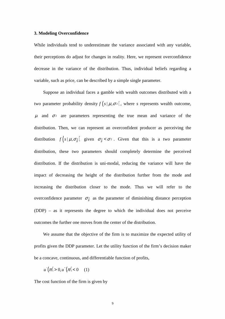
3. Modeling Overconfidence
While individuals tend to underestimate the variance associated with any variable,
their perceptions do adjust for changes in reality. Here, we represent overconfidence
decrease in the variance of the distribution. Thus, individual beliefs regarding a
variable, such as price, can be described by a simple single parameter.
Suppose an individual faces a gamble with wealth outcomes distributed with a
two parameter probability density( )2| ,f s µ σ , where s represents wealth outcome,
µ and 2σ are parameters representing the true mean and variance of the
distribution. Then, we can represent an overconfident producer as perceiving the
distribution ( )2| , gf s µ σ given 2 2gσ σ< . Given that this is a two parameter
distribution, these two parameters should completely determine the perceived
distribution. If the distribution is uni-modal, reducing the variance will have the
impact of decreasing the height of the distribution further from the mode and
increasing the distribution closer to the mode. Thus we will refer to the
overconfidence parameter 2gσ as the parameter of diminishing distance perception
(DDP) – as it represents the degree to which the individual does not perceive
outcomes the further one moves from the center of the distribution.
We assume that the objective of the firm is to maximize the expected utility of
profits given the DDP parameter. Let the utility function of the firm’s decision maker
be a concave, continuous, and differentiable function of profits,
( ) ( ) 0,0 ''' <> ππ uu (1)
The cost function of the firm is given by
10
( ) ( ) BxCxF += (2)
where x is output, ( )xC is the variable cost function, with( ) ( )0 0, ' 0C C x= > , and B
is the fixed cost. The firm’s profit function is thus given by
( ) ( ) BxCpxx −−=π (3)
where p is the price of output, assumed to be random with true density ( )2| ,f p µ σ .
The firm thus maximizes
( )( ) ( )( ) ( )0
| , | ,g g gE u px C x B u px C x B f p dpµ σ µ σ∞
− − = − − ∫ (4)
To proceed, we will use a Taylor-series approximation of the utility function,
( )( ) ( )( ) ( )( ) ( ) ( )( ) ( )22,''2
1,',, µµπµµπµππ −⋅⋅+−⋅⋅+= pxxupxxuxupxu (5)
Thus, the maximization problem can be written as
( )( ) ( )( ) ( ) ( )( ) ( )
( )( ) ( )( ) ( ) ( )( )
22
2 2
1max , ' , '' , | ,
2
1, ' , '' , .
2
g gx
g g
E u x u x x p u x x p
u x u x x u x x
π µ π µ µ π µ µ µ σ
π µ π µ µ µ π µ σ
+ ⋅ ⋅ − + ⋅ ⋅ −
= + ⋅ ⋅ − + ⋅ ⋅
(6)
The first-order condition associated with (7) can be written as
( )( ) ( )( ) ( )( ) ( )( ) ( )
( )( ) ( ) ( )( ) ( )( ) ( )( )2 2 2
' , ' '' , '
1' , ''' , ' '' ,
2
g
g g g
EUu x C x u x C x x
x
u x u x C x x u x x
π µ µ π µ µ µ µ
π µ µ µ π µ µ σ π µ σ
∂ = − + − ⋅ ⋅ −∂
+ − + − ⋅ ⋅ +
(7)
or, dividing by marginal utility
( )( ) ( ) ( )( ) ( ) ( )( )2 2 21
' ' ' 02g A g g A gC x R x C x x P C x xµ µ µ σ µ µ µ µ σ − + − − ⋅ + − ⋅ ⋅ − + − ⋅ ⋅ =
(8)
11
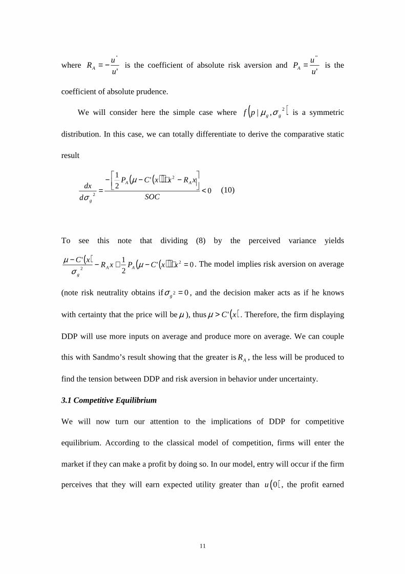
where '
''
u
uRA −= is the coefficient of absolute risk aversion and
'
'''
u
uPA = is the
coefficient of absolute prudence.
We will consider here the simple case where ( )2,| ggpf σµ is a symmetric
distribution. In this case, we can totally differentiate to derive the comparative static
result
( )( )0
'2
1 2
2<
−⋅−−=
SOC
xRxxCP
d
dx AA
g
µ
σ (10)
To see this note that dividing (8) by the perceived variance yields
( ) ( )( ) 0'2
1' 22
=⋅−+−−xxCPxR
xCAA
g
µσ
µ . The model implies risk aversion on average
(note risk neutrality obtains if 2 0gσ = , and the decision maker acts as if he knows
with certainty that the price will beµ ), thus ( )xC '>µ . Therefore, the firm displaying
DDP will use more inputs on average and produce more on average. We can couple
this with Sandmo’s result showing that the greater is AR , the less will be produced to
find the tension between DDP and risk aversion in behavior under uncertainty.
3.1 Competitive Equilibrium
We will now turn our attention to the implications of DDP for competitive
equilibrium. According to the classical model of competition, firms will enter the
market if they can make a profit by doing so. In our model, entry will occur if the firm
perceives that they will earn expected utility greater than ( )0u , the profit earned
12
prior to committing fixed costs. Further, a firm in the industry will shut down
when ( )( ) ( )BuuE −<π . Differentiating with respect to 2gσ obtains
( ) ( )( ) 22
1'' , 0
2g
EUu x x
ππ µ
σ∂
= ⋅ <∂
(10)
Thus, firms with greater DDP (smaller2gσ ) will enter the market, while more rational
firms that perceive correctly the risks they face would consider the expected profit too
small considering the risk involved. This result further supports the result found by
Camerer and Lovallo (1999) that overconfidence leads to greater rates of entry.
However, here we show this in the case of type-2 overconfidence rather than type-1.
Further, this result is well supported by the entrepreneurship literature (e.g., Das and
Teng 1997; Barron 2000) which has uniformly found that entrepreneurs are not more
inclined to take risks, but rather less inclined to take notice of the risks they face. Thus,
as expected profit increases from zero, overconfident decision makers will be the first
into the market and, as expected profits decline below zero, overconfident decision
makers will be the last to shut down.
3.2 Imperfect Competition under Overconfidence
In order to evaluate the effects of DDP on competition, it is necessary to describe the
market. Suppose the inverse demand is given by
( ) ε+= XPP (11),
with ( ) 0' <XP and ( )2,0~ σε , where ∑=
=N
iixX
1
is the total production level in the
market, i is the index of (potential) firms, and N is the number of firms producing.
Differentiating from perfect competition, here price is a function of the total market
13
production X and a random variable ε which captures the price shocks in the
market.
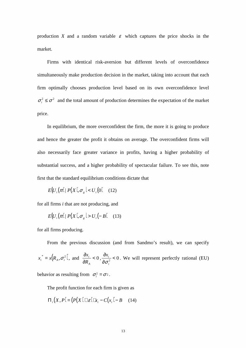
Firms with identical risk-aversion but different levels of overconfidence
simultaneously make production decision in the market, taking into account that each
firm optimally chooses production level based on its own overconfidence level
22 σσ ≤i and the total amount of production determines the expectation of the market
price.
In equilibrium, the more overconfident the firm, the more it is going to produce
and hence the greater the profit it obtains on average. The overconfident firms will
also necessarily face greater variance in profits, having a higher probability of
substantial success, and a higher probability of spectacular failure. To see this, note
first that the standard equilibrium conditions dictate that
( ) ( )( ) ( )0,| igi UXPUE <σπ (12)
for all firms i that are not producing, and
( ) ( )( ) ( )BUXPUE igi −>σπ ,| (13)
for all firms producing.
From the previous discussion (and from Sandmo’s result), we can specify
( )2* , iAi Rxx σ= , and 0<∂∂
A
i
R
x, 0
2<
∂∂
i
ix
σ. We will represent perfectly rational (EU)
behavior as resulting from 2 2iσ σ= .
The profit function for each firm is given as
( ) ( )( ) ( ) BxCxXPPX iii −−⋅+=Π ε, (14)
14
where B is fixed cost. Using a 2-dimensional Taylor expansion, along the production
and price axis, for the utility function, we have
( )[ ] ( )( )[ ]( )( )[ ] ( ) ( ) ( )[ ] ( )( )( )[ ] ( )( )
( )( )[ ] ( ) ( ) ( )[ ] ( )( )( )[ ] ( )( )
( )( )[ ] ( ) ( ) ( )[ ] ( ) ( )( )XPPxxxxCXPxXPXPXu
XPPxXPXu
xxxCXPxXPXPXu
XPPxXPXu
xxxCXPxXPXPXu
XPXuPXu
−⋅−⋅⋅+−+⋅⋅Π+
−Π+
−+−+⋅⋅Π+
−⋅⋅Π+
−⋅+−+⋅⋅Π+
Π=Π
ε
ε
ε
''12
22
22
22''11
2
''1
,
,2
1
,2
1
,
,
,,
(15)
For simplicity, we omit the subscript i letting X denote the total amount of
production in the market and x denote the production level of any arbitrary firm. The
value x is the risk neutral production level and ( )XP is the expectation of the
market price at the risk neutral production level.
Thus, each firm i solves:
( )[ ]( )
( )( )[ ]( )( )[ ] ( ) ( ) ( )[ ] ( )
( )( )[ ] ( ) ( ) ( )[ ]{ } ( ) ( )( )[ ]( ) ( ) ( )[ ] ( ) ( ) ( ) ( )[ ]{ } ( ) KxxxCXPxXPuxxxCXPxXPu
xXPXuxxxCXPxXPXPXu
xxxCXPxXPXPXu
XPXu
PXuE
iiiiiiiii
iiiiiii
iiii
xi
+−⋅+−+⋅⋅+−⋅−+⋅⋅=
Π+−⋅+−+⋅⋅Π+
−⋅−+⋅⋅Π+
Π=
Π
222''11
''1
22
22
222''11
''1
2
1
,2
1,
2
1
,
,
,max
σ
σσ
(16)
Note that since we are dealing exclusively with Type-2 overconfidence,
( ) 0=εE and ( ) ( )XPPE = . Thus the expectation for the third and the last terms of (15)
are 0. Further, the first and the fifth term are merely constants, which we represent
with K, yielding equation (16) above.
15
The first order condition with respect toix can be written as
( ) ( ) ( ) ( ) ( ) ( ){ } ( )22
1 11' ' ' ' 0i i i i i i iu P X x P X C x u P X x P X C x x xσ ⋅ ⋅ + − + ⋅ ⋅ + − + ⋅ − =
(17)
Solving for the optimal output yields
( ) ( ) ( )( ) ( ) ( ){ }
*2
2
' '1
' '
i i
i iA
i i i
P X x P X C xx x
R P X x P X C x σ
⋅ + − = ⋅ +
⋅ + − +
(18)
The level of production *ix is a function of risk-aversion and the level of
overconfidence, ( )2* , iAi Rxx σ= , and 0<∂∂
A
i
R
x, 0
2<
∂∂
i
ix
σ (19).
Expected profit given DDP can be written
( ) ( ) ( ) BxCxXPXE iii −−⋅=Π **** (20)
and thus
( ) ( ) ( )* * * **
' ' 0ii i
i
EP X x P X C x
x
∂ Π = ⋅ + − ≥∂
(21).
Equation (21) follows from Sandmo (1971), i.e. production under uncertainty is
always smaller than that under certainty. First order condition under certainty implies
( ) ( ) ( )' ' 0i iP X x P X C x⋅ + − = , and second order conditions requires that (21) will
hold.
Next, the variance of profit given DDP is given by ( ) ( )2*2*iii xVar ⋅=Π σ , which
is also an increasing function of*ix . Hence, in equilibrium, the more overconfident the
firm, the greater the firm produces and the greater the profit it obtains on average. The
overconfident firms will also necessarily face greater variance in profits, having a
16
higher probability of substantial success, and a higher probability of spectacular
failure, as well.
Based on the above, we can derive the following proposition.
Proposition 1 Let ++ ×⊆ RRF be the set of potential firms, and FFc ⊆ the set of
firms producing under competitive equilibrium. Then, for any( )2, gAR σ , 0>AR
with ( ) cgA FR ∈2,σ , it must be the case that every firm with ( ) cgA FR ∈2',σ
where 22' gg σσ < .
Proof The result follows directly from (19), (20) and (21). Differentiating (20) with
respect to DDP yields
02
*
*
*
2
*
≤∂∂
⋅∂
Π∂=∂
Π∂
i
i
i
i
i
i x
x
EE
σσ. (22)
The result in the above proposition suggests that as long as each decision maker
displays some level of risk aversion, at any level of risk aversion for which a rational
actor produces, every actor with that level of risk aversion (or less) that meets some
minimum level of misperception will operate. If all actors had identical levels of risk
aversion, but varied by DDP, the market would necessarily be dominated by irrational
actors. Rational actors would have a competitive disadvantage in being averse to risk,
and recognizing the level of risk. Alternatively, those who could not see the risk
would invest more heavily and drive more rational investors from the market.
3.3 Ex Post Profits
A possibly more interesting question is what will happen when those with
misperceptions begin to realize their results. Equation (18) can be useful in exploring
the answers to this question. Recall our definition for x as the production level the
17
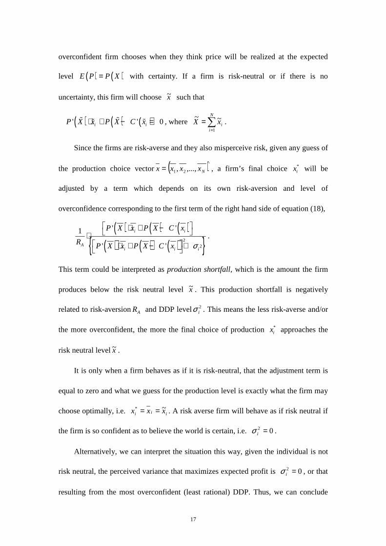
overconfident firm chooses when they think price will be realized at the expected
level ( ) ( )E P P X= with certainty. If a firm is risk-neutral or if there is no
uncertainty, this firm will choose x~ such that
( ) ( ) ( )' ' 0i iP X x P X C x⋅ + − =% %% % , where ∑=
=N
iixX
1
~~.
Since the firms are risk-averse and they also misperceive risk, given any guess of
the production choice vector ( )'
21 ,...,, Nxxxx = , a firm’s final choice *ix will be
adjusted by a term which depends on its own risk-aversion and level of
overconfidence corresponding to the first term of the right hand side of equation (18),
( ) ( ) ( )( ) ( ) ( ){ }2
2
' '1
' '
i i
Ai i i
P X x P X C x
R P X x P X C x σ
⋅ + − ⋅
⋅ + − +
.
This term could be interpreted as production shortfall, which is the amount the firm
produces below the risk neutral level x~ . This production shortfall is negatively
related to risk-aversionAR and DDP level 2iσ . This means the less risk-averse and/or
the more overconfident, the more the final choice of production *ix approaches the
risk neutral levelx~ .
It is only when a firm behaves as if it is risk-neutral, that the adjustment term is
equal to zero and what we guess for the production level is exactly what the firm may
choose optimally, i.e. iii xxx ~* == . A risk averse firm will behave as if risk neutral if
the firm is so confident as to believe the world is certain, i.e. 02 =iσ .
Alternatively, we can interpret the situation this way, given the individual is not
risk neutral, the perceived variance that maximizes expected profit is 02 =iσ , or that
resulting from the most overconfident (least rational) DDP. Thus, we can conclude
18
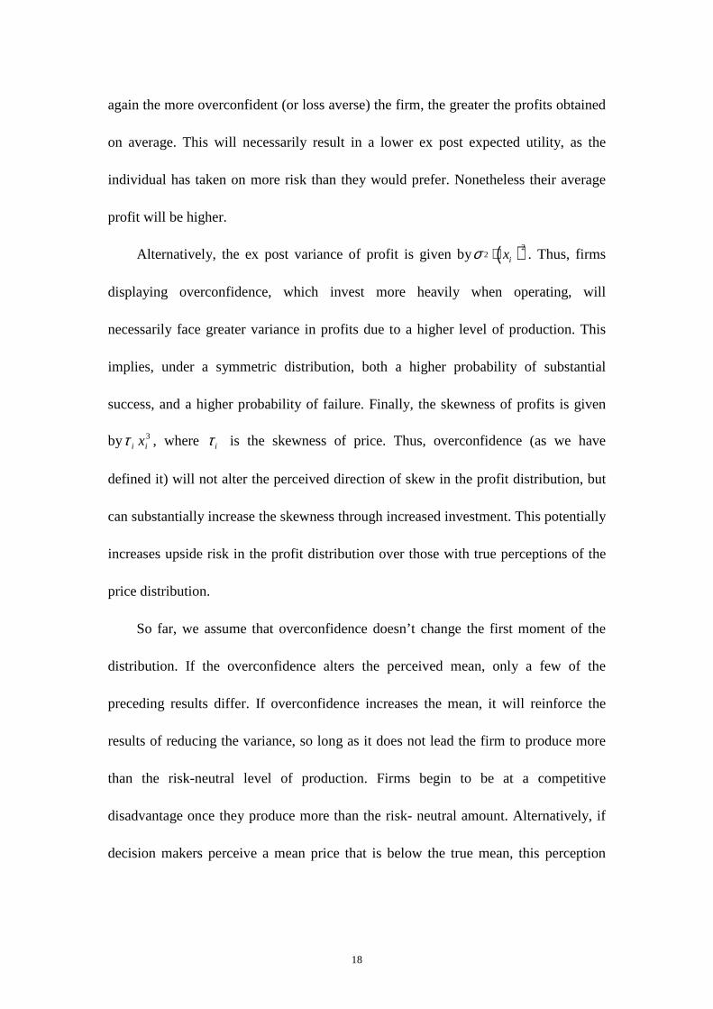
again the more overconfident (or loss averse) the firm, the greater the profits obtained
on average. This will necessarily result in a lower ex post expected utility, as the
individual has taken on more risk than they would prefer. Nonetheless their average
profit will be higher.
Alternatively, the ex post variance of profit is given by ( )22
ixσ ⋅ . Thus, firms
displaying overconfidence, which invest more heavily when operating, will
necessarily face greater variance in profits due to a higher level of production. This
implies, under a symmetric distribution, both a higher probability of substantial
success, and a higher probability of failure. Finally, the skewness of profits is given
by 3ii xτ , where iτ is the skewness of price. Thus, overconfidence (as we have
defined it) will not alter the perceived direction of skew in the profit distribution, but
can substantially increase the skewness through increased investment. This potentially
increases upside risk in the profit distribution over those with true perceptions of the
price distribution.
So far, we assume that overconfidence doesn’t change the first moment of the
distribution. If the overconfidence alters the perceived mean, only a few of the
preceding results differ. If overconfidence increases the mean, it will reinforce the
results of reducing the variance, so long as it does not lead the firm to produce more
than the risk-neutral level of production. Firms begin to be at a competitive
disadvantage once they produce more than the risk- neutral amount. Alternatively, if
decision makers perceive a mean price that is below the true mean, this perception
19
will work against the reduction in perceived variance, reducing the amount produced,
and placing the firm at a competitive disadvantage.
4. Welfare Analysis
Finally, one may wonder about the welfare effects of overconfidence. This is easiest
to consider by comparing equilibria consisting of identical actors. Clearly, because
overconfidence leads to greater production for all levels of expected prices,
consumers must benefit from the resultant lower equilibrium price. On the other
hand, producers necessarily obtain lower utility of profit on average than they
anticipate, meaning they could be made better off. The ex post producer surplus must
disregard overconfidence, calculating the true average net benefit. This necessarily
declines as variance is misperceived at a rate determined by the degree of risk
aversion. If actors were truly risk neutral, misperceptions of variance would not
matter to producers. Alternatively, if producers are very risk averse, misperceptions of
variance could reduce producer surplus by more than the increase in consumer surplus
leading to a market failure. Thus, if firms are only mildly risk averse, there may exist
some socially optimal level of overconfidence. On the other hand, if firms were
severely risk averse, the government may have a role in reducing overconfidence
(through education, market publications, etc.) or reducing risk (through disaster relief)
to improve welfare of producers.
From the previous section we have
( ) ( )( ) ( ) BXCxXPPX ii −−⋅+=Π ε, , where ∑=
=N
iixX
1
and ( )2,0~ σε .
20
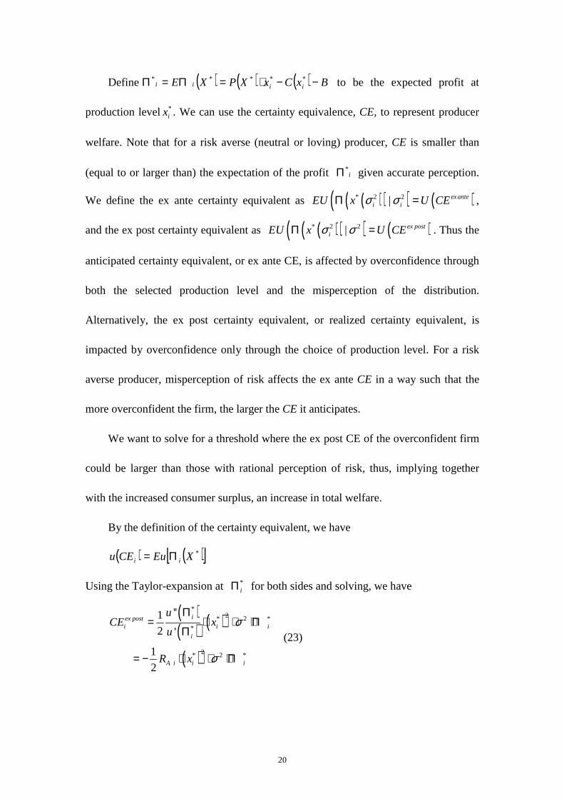
Define ( ) ( ) ( ) BxCxXPXE iiii −−⋅=Π=Π ***** to be the expected profit at
production level *ix . We can use the certainty equivalence, CE, to represent producer
welfare. Note that for a risk averse (neutral or loving) producer, CE is smaller than
(equal to or larger than) the expectation of the profit i*Π given accurate perception.
We define the ex ante certainty equivalent as ( )( )( ) ( )* 2 2| ex antei iEU x U CEσ σΠ = ,
and the ex post certainty equivalent as ( )( )( ) ( )* 2 2| ex postiEU x U CEσ σΠ = . Thus the
anticipated certainty equivalent, or ex ante CE, is affected by overconfidence through
both the selected production level and the misperception of the distribution.
Alternatively, the ex post certainty equivalent, or realized certainty equivalent, is
impacted by overconfidence only through the choice of production level. For a risk
averse producer, misperception of risk affects the ex ante CE in a way such that the
more overconfident the firm, the larger the CE it anticipates.
We want to solve for a threshold where the ex post CE of the overconfident firm
could be larger than those with rational perception of risk, thus, implying together
with the increased consumer surplus, an increase in total welfare.
By the definition of the certainty equivalent, we have
( ) ( )[ ]*XEuCEu ii Π=
Using the Taylor-expansion at *iΠ for both sides and solving, we have
( )( ) ( )
( )
*2* 2 *
*
2* 2 *
''1
2 '
1
2
iex posti i i
i
A i i i
uCE x
u
R x
σ
σ
Π= ⋅ ⋅ + Π
Π
= − ⋅ ⋅ + Π
(23)
21
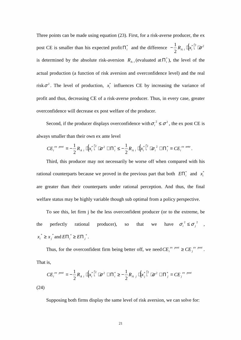
Three points can be made using equation (23). First, for a risk-averse producer, the ex
post CE is smaller than his expected profit*iΠ and the difference ( ) 22*
2
1 σ⋅⋅− iiA xR
is determined by the absolute risk-aversion iAR (evaluated at *iΠ ), the level of the
actual production (a function of risk aversion and overconfidence level) and the real
risk 2σ . The level of production, *ix influences CE by increasing the variance of
profit and thus, decreasing CE of a risk-averse producer. Thus, in every case, greater
overconfidence will decrease ex post welfare of the producer.
Second, if the producer displays overconfidence with 22 σσ ≤i , the ex post CE is
always smaller than their own ex ante level
( ) ( ) anteexiiiiiAiiiA
postexi CExRxRCE =Π+⋅⋅−≤Π+⋅⋅−= *22**22*
2
1
2
1 σσ .
Third, this producer may not necessarily be worse off when compared with his
rational counterparts because we proved in the previous part that both *iEΠ and *
ix
are greater than their counterparts under rational perception. And thus, the final
welfare status may be highly variable though sub optimal from a policy perspective.
To see this, let firm j be the less overconfident producer (or to the extreme, be
the perfectly rational producer), so that we have 22ji σσ ≤ ,
**ji xx ≥ and * *
i jE EΠ ≥ Π .
Thus, for the overconfident firm being better off, we need postexj
postexi CECE ≥ .
That is,
( ) ( ) postexjjjjAiiiA
postexi CExRxRCE =Π+⋅⋅−≥Π+⋅⋅−= *22**22*
2
1
2
1 σσ
(24)
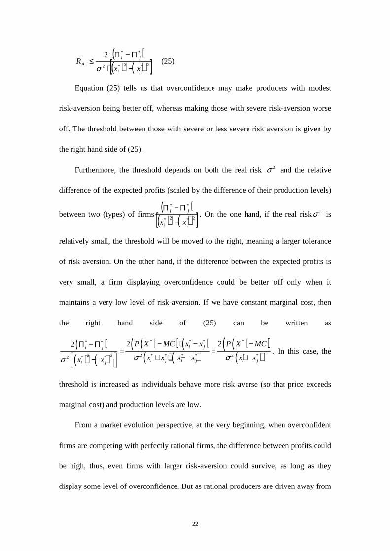
Supposing both firms display the same level of risk aversion, we can solve for:
22
( )( ) ( )[ ]2*2*2
**2
ji
jiA
xxR
−⋅
Π−Π⋅≤
σ (25)
Equation (25) tells us that overconfidence may make producers with modest
risk-aversion being better off, whereas making those with severe risk-aversion worse
off. The threshold between those with severe or less severe risk aversion is given by
the right hand side of (25).
Furthermore, the threshold depends on both the real risk 2σ and the relative
difference of the expected profits (scaled by the difference of their production levels)
between two (types) of firms( )
( ) ( )[ ]2*2*
**
ji
ji
xx −
Π−Π. On the one hand, if the real risk2σ is
relatively small, the threshold will be moved to the right, meaning a larger tolerance
of risk-aversion. On the other hand, if the difference between the expected profits is
very small, a firm displaying overconfidence could be better off only when it
maintains a very low level of risk-aversion. If we have constant marginal cost, then
the right hand side of (25) can be written as
( )( ) ( )
( )( ) ( )( ) ( )
( )( )( )
* * * ** *
2 2 2 * * * * 2 * *2 * *
2 22 i ji j
i j i j i ji j
P X MC x x P X MC
x x x x x xx x σ σσ
− ⋅ − −Π − Π= =
+ ⋅ − +−
. In this case, the
threshold is increased as individuals behave more risk averse (so that price exceeds
marginal cost) and production levels are low.
From a market evolution perspective, at the very beginning, when overconfident
firms are competing with perfectly rational firms, the difference between profits could
be high, thus, even firms with larger risk-aversion could survive, as long as they
display some level of overconfidence. But as rational producers are driven away from
23
the market, the gap between profits shrinks, since all firms are now overconfident, and
they differ only by the levels of their misperception. And hence, firm with a low level
of risk-aversion is better off. Or, for a certain level of risk-aversion, a firm can only
survive the market by displaying even greater level of overconfidence and performing
as if he is as close to risk-neutral as possible. This may explain how overconfidence
could persist in the long run.
5. Model Impacts of Overconfidence on Production
Previous work has shown that overconfidence may persist in financial trading, as well
as cause entry. Our results suggest that overconfidence may be a natural result of
market pressures, and may thus persist in a competitive production market. While all
would agree that starting a new business is an extremely risky venture, there is little
evidence that entrepreneurs are more risk tolerant than other individuals (Palich and
Bagby (1995)). In fact, Low and MacMillan (1988) find specifically that propensity to
take on risk does not differentiate entrepreneurs from nonentrepreneurs. Rather, many
have discovered that entrepreneurs differ in the process by which they evaluate
opportunities and assess the risks involved (Das and Teng (1997), Cooper, Woo, and
Dunkelberg (1988), Forlani and Mullins (2000)). For example, Baron (2000) finds
that entrepreneurs are less likely to engage in counterfactual thinking, not recognizing
the possibility for alternative outcomes of their venture.
Many have found an empirical link between the underestimation of risk and
entrepreneurship activity (see, for example, Simon, Houghton, and Aquino (2000)).
Camerer and Lovallo (1999) use economic theory to argue that such overconfidence
24
should lead to excess entrepreneurial activity. Despite an increasingly evident link
between overconfidence and entrepreneurship, little is known of the effects of
overconfidence on business performance under competition. In this paper, we follow
the analysis of Sandmo (1971), applying the principles of DDP and EU maximization
to examine the effects of competition on firms displaying overconfidence. We show
that overconfidence may not only lead to excessive entry, but also give entrepreneurs
a competitive edge not achieved by more rational decision makers. Our result may
also explain the recent results of Bogan and Just (forthcoming) suggesting that CEOs
are display greater confirmation bias and overconfidence than other populations. They
show that this may be behind excessive merger activity. Overconfidence can create a
competitive advantage in production decisions. But the same behavioral anomaly that
makes a CEO desirable for competitive production may make them the wrong person
for the job when it comes to merger decisions.
6. Conclusion
While many have published proofs that competition forces rationality (see, for
example, Green (1987)), this paper provides a rationale for why non-rational models
may be relevant even in highly competitive industries. In fact, it seems clear that DDP,
while irrational, creates a competitive advantage, and thus markets may be dominated
by this particular brand of irrationality. The fact that competition may encourage such
behavior in the face of risk aversion makes it a little more understandable why such
behavior may pop up in experimental settings. Further, empirical assessments in the
entrepreneurship literature suggest that behavioral phenomena such as DDP may play
25
a larger role in entry decisions than factors like DMUW that are more commonly
considered. There is little reason to believe that competition will sort DDP from the
market, and thus DDP may also play a large role in production level decisions and
exit from a competitive industry. The work in this paper provides a neoclassical
economic argument for why this patently non-classical phenomenon should exist and
persist and why behavioral effects may be important. Those who underestimate risk
are likely to invest more, increasing their chances for greater success (or failure) than
can be realized with a rational view of the world.
References
[1] D. Ahler and J. Lakonishok, A study of economists’ consensus forecasts,
Management Science, 29 (1983), 1113-1125.
[2] A.M. Allais, Le comportement de l'homme rationnel devant le risque, critique des
postulats et axiomes del l'ecole Americaine, Econometrica 21 (1953), 503–546.
[3] M. Alpert, H. Raiffa, A progress report on the training of probability assessors, in:
D. Kahneman, P. Slovic, A. Tversky (Eds.), Judgment Bias under Uncertainty:
Heuristics and Biases, Cambridge University Press, New York, 1982.
[4] K. Arrow, Essays on the Theory of Risk Bearing. Markham Press, New York,
1971.
[5] L. M. Ausubel, The failure of competition in the credit card market, American
Economic Review 81 (1991), 50-81.
[6] R.A. Baron, Counterfactual thinking and venture formation: The potential effects
of thinking about ‘what might have been,’ J. Bus. Venturing 15 (2000), 79–91.
26
[7] C. Camerer, D. Lovallo, Overconfidence and excess entry: An experimental
approach, Amer. Econ. Rev. 89 (1999), 306–318.
[8] S.H. Chew, A generalization of the quasilinear mean with applications to the
measurement of income inequality and decision theory resolving the Allais
Paradox, Econometrica 51 (1983), 1065–1092.
[9] S.H. Chew, W. Waller, Empirical tests of weighted utility theory, J. Math. Psych.
30 (1986), 55–72.
[10] A.C. Cooper, C.Y. Woo, W.C. Dunkelberg, Entrepreneurs’ perceived chance of
success, J. Bus. Venturing 3 (1988), 97–108.
[11] T. K. Das, B.S. Teng, Time and entrepreneurial risk behavior, Entrepreneurship
Theory and Practice 22 (1997), 69–88.
[12] W. F. M. De Bondt and R. H. Thaler, Do security analysts overact? American
Economic Review 80 (1990), 52-57.
[13] W. F. M. De Bondt, What do economists know about the stock market? Journal
of Portfolio Management 17 (1991), 84-91.
[14] E. J. Elton, M. J. Gruber and M. N. Gültekin, Professional expectations:
Accuracy and diagnosis of errors, Journal of Financial and Quantitative Analysis
19 (1984), 351-365.
[15] G. Feder, The impact of uncertainty in a class of objective functions, J. Econ.
Theory 16 (1977), 504–512.
[16] D. Forlani, J.W. Mullins, Perceived risks and choices in entrepreneurs’ new
venture decisions, J. Bus. Venturing 5 (2000), 305–322.
27
[17] K. A. Froot and J. A. Frankel, Forward discount bias: Is it an exchange risk
premium? Quarterly Journal of Economics 104 (1989), 139-161.
[18] J. Green, Making book against oneself, the independence axiom, and nonlinear
utility theory, Quart., J. Econ. 102 (1987), 785–796.
[19] J.D. Hey, C. Orme, Investigating generalizations of expected utility theory using
experimental data, Econometrica 62 (1994), 1291–1326.
[20] H.K. Hvide, Pragmatic beliefs and overconfidence, Journal of Economic
Behavior and Organization 48 (2002), 15–28.
[21] D. Kahneman, A. Tversky, Prospect theory: An analysis of decision under risk,
Econometrica 47 (1979), 263–292.
[22] A. Kyle, F. A. Wang, Speculation duopoly with Agreement to Disagree: Can
overconfidence survive the market test? Journal of Finance 52 (1997),
2073-2089.
[23] M.B. Low, I.C. MacMillan, Entrepreneurship: Past research and future
challenges, Journal of Management. 14 (1988), 139–161.
[24] W. Nielson, Calibration results for rank-dependent expected utility, Econ.
Bulletin 4 (2001), 1–5.
[25] T. O’Dean, Volume, volatility, price and profit when all traders are above
average, working paper No. RPF-266 (1997), University of California at
Berkeley..
[26] T. O’Dean, B.M. Barber, Boys will be boys: Gender, overconfidence, and
common stock investment, Quart. J. Econ. 115 (2001), 261–283.
28
[27] S. Oskamp, Overconfidence in case-study judgments, J. Consulting Psych. 29
(1965), 261–265.
[28] L.E. Palich, D.R. Bagby, Using cognitive theory to explain entrepreneurial
risk-taking: Challenging conventional wisdom, J. Bus. Venturing 10 (1995),
425–438.
[29] J.W. Pratt, Risk aversion in the small and in the large, Econometrica 32 (1964),
122–136.
[30] M. Rabin, Risk aversion and expected-utility theory: A calibration theorem,
Econometrica 68 (2000), 1281–1292.
[31] J. Russo and P. Schoemaker, Managing overconfidence, Sloan Management
Review, 33 (1992), 7-17.
[32] A. Sandmo, On the theory of the competitive firm under price uncertainty, Amer.
Econ. Rev. 61 (1971), 65–73.
[33] M. Simon, S. M. Houghton, K. Aquino, Cognitive biases, risk perception and
venture formation: How individuals decide to start companies, J. of Bus.
Venturing 15 (2000), 113–134.
[34] C. Staël von Holstein, Probabilistic forecasting: An experiment related to the
stock market, Organizational Behavior and Human Performance, 8 (1972),
139-158.
[35] C. Starmer, Developments in non-expected utility theory: The hunt for a
descriptive theory of choice under risk, J. of Econ. Lit. 38 (2000), 332–382.
29
[36] O. Svenson, Are we all less risky and more skillful than our fellow drivers?, Acta
Pshchologica, 47 (1981), 143-148.
[37] S. Taylor and J. Brown, Illusion and well-being: A social psychological
perspective on mental health, Psychological Bulletin, 103 (1988), 193-210.
[38] A. Tversky, D. Kahneman, Advances in prospect theory: Cumulative
representation of uncertainty, J. of Risk and Uncertainty 5 (1992), 297–323.
[39] A. Tversky, D. Kahneman, Judgment under uncertainty: Heuristics and biases,
Science 185 (1974), 1124-1131.
[40] W.K. Viscusi, Prospective reference theory: Toward an explanation of the
paradoxes, J. of Risk and Uncertainty 2 (1989), 235–264.
[41] W. Wagenaar and G. Keren, Does the expert know? The reliability of predictions
and confidence ratings of experts, In eds. E. Hollnagel, G. Maneini, and D.
Woods, Intelligent Decision Support in Process Environments, Berlin: Springer,
87-107.
[42] P. Wakker, D. Deneffe, Eliciting von Neumann-Morgenstern utilities when
probabilities are distorted or unknown, Manage. Science 42 (1996), 1131-1150.
[43] N. Weinstein, Unrealistic optimism about future life events, Journal of
Personality and Social Psychology, 49 (1980), 806-820.