Risk and Insurance in Village India

1/ 31

Risk and Insurance in Village India

Robert M. Townsend (1994)

Presented by Chi-hung Kang

November 14, 2016

Robert M. Townsend (1994) Risk and Insurance in Village India November 14, 2016 1 / 31

2/ 31

Motivation

Poor agricultural villages in Southern India face high risk fromweather and crop diseases

I Are landless labors more vulnerable than the landlords?

I Does consumption fluctuate with the income shocks?

I Are people fully insured at the village level?

I Which economic activity is better insured?

Is there any scope for policy reform?


3/ 31

Data

Data of southern India villages from International Crops ResearchInstitute of the Semi-Arid Tropics (ICRISAT)

I Annual data 1975–1984

I Three villages: Aurepalle, Shirapur, Kanzara

I 40 households for each village

I Panel data for 35, 32, 36 households respectively


4/ 31

Table I: Composition of Income


5/ 31

Figure 1 and Figure 3: Deviation From the Village Average

Deviation of individual income from the village average income isquite volatile

Deviation of individual consumption from the village averageconsumption is relatively small


6/ 31

Prediction From the Model

Proposition

By Wilson (1968) and Diamond (1967), if the following assumptions hold,

1 Preferences are time separable

2 Weak risk aversion

3 All individuals have the same discount rate

4 All information is held in common

then a Pareto optimal allocation of risk bearing of a single good in astochastic environment implies that all individual consumption isdetermined by aggregate consumption

Idiosyncratic shocks should not influence individual consumption

The implication holds in a multiple commodity world under separablepreferences


7/ 31

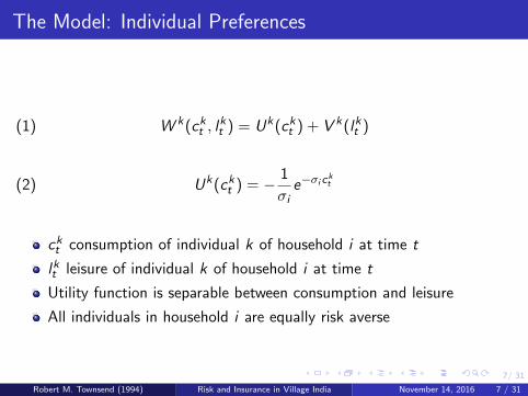
The Model: Individual Preferences

(1) W k(ckt , lkt ) = Uk(ckt ) + V k(lkt )

(2) Uk(ckt ) = − 1

σie−σic

kt

ckt consumption of individual k of household i at time t

lkt leisure of individual k of household i at time t

Utility function is separable between consumption and leisure

All individuals in household i are equally risk averse


8/ 31

The Model: Household Decision

For a househould i with M individuals, the maximization problem is:

maxM∑k=1

λk

(T∑t=1

βtE0

[Uk(ckt ) + V k(lkt )

])

s.t.M∑k=1

ckt ≤ c̄t ;M∑k=1

lkt ≤ l̄t ,

ckt ≥ 0; 0 ≤ lkt ≤ T kt ,

0 < λk < 1,M∑k=1

λk = 1

λk is the utility weight of individual k in the household


9/ 31


For any two individuals k and j in household i at time t, the weightedmarginal utility should be the same to achieve Pareto optimal within thehousehold:

λk∂Uk

∂ckt= λj

∂U j

∂c jt= µc

µc Lagrange multiplier for consumption constraint


10/ 31


Assume that σi = σ, summing over the FOC of total individuals inhousehold i and total households N in the village gives Pareto optimalconsumption of household i :

(3) c it =1

N it

N it∑

k=1

ckt = − 1

σ

(ln(λi ) − 1

N

N∑i=1

ln(λi )

)+ c̄t

c̄t =1

N

N∑i=1

c it

Assume that λi are the same for each household, then

(4) c it = c̄t


11/ 31

Equivalence Scales

c it is adjusted by household size

I Is c it =∑Ni

tk=1 c

kt

N it

a good adjustment ?

Deaton (2003) Simply deflating by total household size has two majorproblems

I Ignoring the household composition

I Ignoring any economies of scale in consumption within the household;“public goods” of the household

Browning, Chiappori and Lewbel (2010)

I Equivalence scales measure the ratio of costs of attaining the sameutility level


12/ 31

Equivalence Scales

Construct the equivalence scale Akt for individual k at time t

according to the caloric intake from the survey of Ryan, Bidinger,Pushpamma and Rao (1985)

Age-sex categories Equivalence Scales

Adult Males 1.00Adult Females 0.90Males aged 13–18 0.94Females aged 13–18 0.83Children aged 7–12 0.67Children aged 4–6 0.52Toddlers 0.32Infants 0.05


13/ 31


Incorporate the equivalence scale Akt in the individual utility function:

W k(ckt , lkt ,A

kt ) = Uk(ckt ,A

kt ) + V k(lkt ,A

kt )

Uk(ckt ,Akt ) = − 1

σie−σi c

kt

Akt ,

∂Uk

∂Akt

= − ckt(Ak

t )2e−σi c

kt

Akt < 0

Given the same consumption, with a higher equivalence scale Akt ,

individual k has a lower utility level.


14/ 31


The Pareto optimal consumption of household i can be rewritten as:

(5) c∗it = c̄t −1

σAit

c∗it =

N it∑

k=1

ckt

N it∑

k=1

Akt

, c̄t =1

N

N∑i=1

c∗it


15/ 31


Where Ait is defined as:

(6) Ait =

N i∑k=1

Akt ln(Ak

t )

N i∑k=1

Akt

− 1

N

N∑i=1

N i∑k=1

Akt ln(Ak

t )

N i∑k=1

Akt


16/ 31

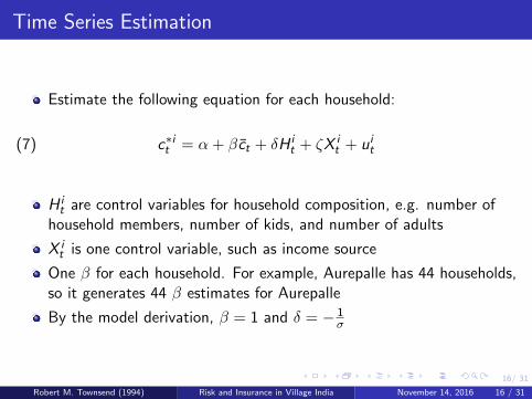
Time Series Estimation

Estimate the following equation for each household:

(7) c∗it = α + βc̄t + δH it + ζX i

t + uit

H it are control variables for household composition, e.g. number of

household members, number of kids, and number of adults

X it is one control variable, such as income source

One β for each household. For example, Aurepalle has 44 households,so it generates 44 β estimates for Aurepalle

By the model derivation, β = 1 and δ = − 1σ


17/ 31

Figure 5: Time Series Estimates

For each village, rank households according to the magnitude of β.The dots in the figure are β for each household i , and the lines are95% confidence interval


18/ 31

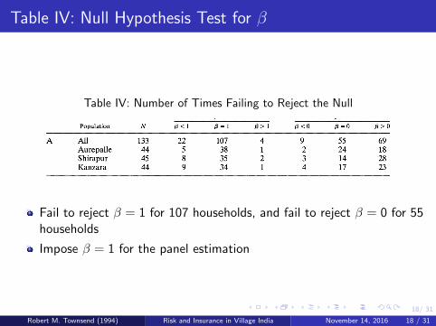
Table IV: Null Hypothesis Test for β

Table IV: Number of Times Failing to Reject the Null

Fail to reject β = 1 for 107 households, and fail to reject β = 0 for 55households

Impose β = 1 for the panel estimation


19/ 31

Panel Estimation

Fixed effect estimation:

(8) c∗it − c̄t = αi + δH it + ζwX

it + e it

First-difference estimation

(9) ∆c∗it − ∆c̄t = δ∆H it + ζ i∆∆X i

t + ∆e it

I αi is household fixed effect

I H it are the control variables for household composition, e.g. Number of

household members, number of kids, number of adults

I X it is one control variable

I ζ iw Within-village estimate

I ζ i∆ First-difference estimate

I Regress with one control variable each time


20/ 31

Table VIII: Panel Estimates From Equation (8) and (9)

One coefficient represents one regression


21/ 31

Panel Estimation: Control for All Income Sources

Fixed effect estimation with income sources:

(10) c∗it − c̄t = αi + δH it + ζwX

it + Y i

t Γ + e it

H it are the controls of household composition

X it average village labors

Y it is a vector of income variables, including crop profit, labor income,

trade and handicrafts, and animal husbandry

If the consumption is fully insured against income shocks, thecoefficients of income variables should be jointly zero


22/ 31

Table IX: Control for All Income Sources


23/ 31

Effect of Landholding on Insurance

Estimate the effect of village consumption on the landless household `

(11) c∗`t = α` + βc̄t + δH`t + γy `t + u`t

α` is household fixed effect

H`t are the controls for household composition

y `t all income of landless household `

β = 1 if the idiosyncratic shocks are fully insured at the village level

γ = 0 if the income shocks are fully insured


24/ 31

Table X: Effect of Landholding on Insurance


25/ 31

Kinship and Financial Networks, Formal FinancialAccess, and Risk Reduction

Cynthia Kinnan and Robert Townsend (2012)

Presented by Chi-hung Kang

November 14, 2016

Kinnan and Townsend (2012) Financial Networks and Risk Reduction November 14, 2016 25 / 31

26/ 31

Motivation

Access to borrowing and lending can be helpful to insure againstshort-term idiosyncratic risks

I Informal credit: borrowing from relatives

I Formal financial institution: banks

What are the effect of these two channels on consumption smoothing?


27/ 31

Consumption-smoothing specification

∆civt =α1∆yivt + α2∆yivt di ,B + α3∆yivt ri ,B

+ α4∆yivt ki + α5∆yivt w̄i + δB,t + εit

∆civt Difference of consumption for household i in village v at time t

∆yivt Difference of income for household i in village v at time t

di ,B = 1 if i borrows directly from the bank

ri ,B = 1 if i borrows from someone who borrows from the bank

ki = 1 if having any kin in the village

w̄i household i ’s average net worth over the sample period

δB,t common time effect of households directly connected to the bank


28/ 31

Result for Consumption-smoothing specification

∆civt =0.0078∆yivt − 0.1658∆yivt di ,B − 0.1643∆yivt ri ,B

+ 0.0102∆yivt ki − 0.00021∆yivt w̄i + δB,t + εit

∆civt Difference of consumption for household i in village v at time t

∆yivt Difference of income for household i in village v at time t

di ,B = 1 if i borrows directly from the bank






29/ 31

Investment-smoothing specification

( I

A

)ivt

=α1

( yA

)ivt

+ α2

( yA

)ivt

ri ,B + α4

( yA

)ivt

ki + α5

( yA

)ivt

w̄i

+ β1ri ,B + β2ki ,B + β3w̄i + δv + δB,t + εit

I is total household investment

y is total household income

A is total household assets




δv village fixed effect



30/ 31

Table 1: Kinship, Financial Access, and Investment


31/ 31

Extension

An indicator for having a kin in the village does not capture the wholeeffects of personal networks

I Network characteristics rather than just an indicator

The indicator for direct connection to the bank can be endogenous

I For US data, use the total banks around the neighborhood as a proxyfor formal financial access


Risk and Insurance in Village India

Documents

Transcript of Risk and Insurance in Village India