1

Risk Aggregation in the presence of Discrete Causally

Connected Random Variables

Peng Lin†, Martin Neil† and Norman Fenton†

ABSTRACT

Risk aggregation is a popular method used to estimate the sum of a collection of finan-

cial assets or events, where each asset or event is modelled as a random variable. Appli-

cations include insurance, operational risk, stress testing, and sensitivity analysis. In

practice the sum of a set of random variables involves the use of two well-known math-

ematical operations: n-fold convolution (for a fixed number n) and N-fold convolution,

defined as the compound sum of a frequency distribution N and a severity distribution,

where the number of constant n-fold convolutions is determined by N. Where the severi-

ty and frequency variables are independent, and continuous, currently numerical solu-

tions such as, Panjer’s recursion, Fast Fourier transforms and Monte Carlo simulation

produce acceptable results. However, they have not been designed to cope with new

modelling challenges that require hybrid models containing discrete explanatory (regime

switching) variables or where discrete and continuous variables are inter-dependent and

may influence the severity and frequency in complex, non-linear, ways. This paper de-

scribes a Bayesian Factorization and Elimination (BFE) algorithm that performs convo-

lution on the hybrid models required to aggregate risk in the presence of causal depend-

encies. This algorithm exploits a number of advances from the field of Bayesian Net-

works, covering methods to approximate statistical and conditionally deterministic func-

tions to factorize multivariate distributions for efficient computation. Experiments show

that BFE is as accurate on conventional problems as competing methods. For more diffi-

cult hybrid problems BFE can provide a more general solution that the others cannot of-

fer. Additionally, the BFE approach can be easily extended to perform deconvolution for

† Peng Lin, PhD candidate, Department of Computer Science, Queen Mary, University of London, UK,

p.lin@eecs.qmul.ac.uk † Martin Neil, Professor of Computer Science and Statistics, Department of Computer Science, Queen Mary, Universi-

ty of London, UK, martin@eecs.qmul.ac.uk † Norman Fenton, Professor of Computer Science, Department of Computer Science, Queen Mary, University of Lon-

don, UK, norman@eecs.qmul.ac.uk

2

the purposes of stress testing and sensitivity analysis in a way that competing methods do

not.

Keywords: Risk aggregation; Bayesian Factorization and Elimination; Convolution; De-

convolution; Causal dependency modelling; Bayesian networks; Dynamic Discretization.

1. MOTIVATION AND INTRODUCTION

Risk aggregation is a popular method used to estimate the sum of a collection of fi-

nancial assets or events, where each asset or event is modelled as a random variable. Ex-

isting techniques make a number of assumptions about these random variables. Firstly,

they are almost always continuous. Secondly, if they are independent then they are iden-

tically distributed. Thirdly, should they be dependent, these dependencies are best repre-

sented by correlation functions, such as copulas (Embrechts, 2009) (Nelsen, 2007),

where marginal distribution functions are linked by some dependence structure. These

statistical methods have tended to model associations between variables as a purely phe-

nomenological artefact extant in historical statistical data. Recent experience, at least

since the beginning of the financial crisis in 2007, has amply demonstrated the inability

of these assumptions to handle non-linear effects or “shocks” on financial assets and

events, resulting in models that are inadequate for prediction, stress testing and model

comprehension (IMF, 2009), (Laeven & Valencia, 2008).

It has been extensively argued that modelling dependence as correlation is insuffi-

cient, since it ignores any views that the analyst may, quite properly, hold about those

causal influences that help generate and explain the statistical data observed (Meucci,

2008), (Rebonato, 2010). Such causal influences are commonplace and permeate all lev-

els of economic and financial discourse. For example, does a dramatic fall in equity pric-

es cause an increase in equity implied volatilities or is it an increase in implied volatility

that causes a fall in equity prices? The answer is trivial in this case, since a fall in equity

prices is well known to affect implied volatility, but correlation alone contains no infor-

mation about the direction of causation. To incorporate causation we need to involve the

analyst or expert and “fold into” the model views of how discrete events interact and the

3

effects of this interaction on the aggregation of risk. This approach extends the methodo-

logical boundaries last pushed back by the celebrated Black–Litterman model (Black &

Litterman, 1991). In that approach a risk manager’s role is as an active participant in the

risk modelling, and the role of the model is to accommodate their subjective “views”,

expressed as Bayesian priors of expectations and variances of asset returns. In this paper

we aim to represent these Bayesian “views” in an explicit causal structure, whilst provid-

ing the computational framework for solutions. Such causal models would involve dis-

crete explanatory (regime switching) variables and hybrid mixtures of inter-dependent

discrete and continuous variables. A causal risk aggregation model might incorporate

expert derived views about macro-economic, behavioural, operational or strategic factors

that might influence the assets or events under “normal” or “abnormal” conditions. Ap-

plications of the approach include insurance, stress testing, operational risk and sensitivi-

ty analysis.

At its heart risk aggregation requires the sum of n random variables. In practice this in-

volves the use of two well-known mathematical operations: n-fold convolution (for a

fixed value of n ) and N-fold convolution (Heckman & Meyers, 1983), defined as the

compound sum of a frequency distribution, N , and a severity distribution, S , where the

number of constant n-fold convolutions is determined by N , stochastically. Currently

popular methods such as Panjer’s recursion (Panjer 1981), Fast Fourier transforms

(Heckman and Meyers 1983) and Monte Carlo simulation (Meyers 1980) perform risk

aggregation numerically using parameters derived from historical data to estimate the

distributions for both S and N . Where S and N are independent, and continuous,

these approaches produce acceptable results. However, they have not been designed to

cope with the new modelling challenges outlined above. In the context of modelling gen-

eral dependencies among severity variables, a popular approach is to use copulas, , both

to model the dependent variables and to perform risk aggregation.

Our aim then is to show how we can carry out a stochastic risk aggregation (N-fold

convolution) in a causal Bayesian framework, in such a way that subjective views about

inter-dependencies can be explicitly modelled and numerically evaluated i.e. where dis-

crete and continuous variables are inter-dependent and may influence N and S in com-

4

plex, non-linear ways. We see this as the first of many financial modelling problems that

are amenable to this new approach.

This paper describes a Bayesian Factorization and Elimination (BFE) algorithm that

performs convolution on the hybrid models required to aggregate risk in the presence of

causal dependencies. This algorithm exploits a number of advances from the field of

Bayesian Networks (BNs), covering methods to approximate statistical and conditionally

deterministic functions and to factorize multivariate distributions for efficient computa-

tion.

Section 2 provides an overview of popular methods for risk aggregation. Section 3

describes BN technology with a view to explaining some of the core foundational algo-

rithms used in this paper. The BFE convolution algorithm is described in Section 4,

showing how it builds and extends on the standard BN algorithms presented in Section 3.

Section 5 presents a version of BFE that performs deconvolution and Section 6 presents

experimental results showing the performance of BFE. Section 7 concludes the paper.

2. RISK AGGREGATION

An encyclopaedic overview of the current state of the art in risk aggregation is pre-

sented in , (McNeil, Frey, & Embrechts, 2010). The general aggregation formula for

fixed, n , assets, is:

0 1 ... nT S S S (2.1)

where T is the sum of n asset valuations and each iS is from the same common contin-

uous distribution xf , which can be thought of as a return (severity) distribution S . This

is called an n-fold convolution. If ~ xS f and if we have a variable number of assets, N ,

then (2.1) can be rewritten as an N-fold convolution:

*

0

( ) ( ) ( )j

T

j

f x f x P N j

(2.2)

5

where * *( 1)

0

( ) ( ) ( )j jf x f x y f dy

is a recursive n-fold convolution on S . We

can therefore rewrite (2.2) in a discrete form: ( ) jP N j a , for 0,1,...,j L , where L

is the length of discretized frequency N . The following expressions hold:

0 0 1 1( ) ( ) ( ) ... ( )L LP T a P T a P T a P T (2.3)

0 0 1 0 1 0 1, ,..., ...L LT S T S S T S S S (2.4)

where each jT is a constant n-fold convolution. The formula (2.3) represents a mix-

ture distribution where the mixture components consist of mutually exclusive variables,

themselves composed using the conditionally deterministic functions stated in (2.4).

For the sake of clarity in insurance, and similar, applications N is interpreted as a

frequency distribution, and S is defined as a severity (loss) distribution.

General numerical solutions to computing the aggregate distribution include Pan-

jer’s recursion (Panjer, 1981), Fast Fourier transform (Heckman & Meyers, 1983). and

Monte Carlo (MC) simulation (Meyers, 1980).

In this paper severity variables can depend on discrete explanatory variables with

dependencies expressed via conditioning in Bayesian networks. This contrasts with the

classic approach for dependency modelling among severity variables using copulas. Ra-

ther than use dependency and conditioning the copula approach models the dependency

structure independently with marginal functions, which supports the construction of high

dimensional models.

In the context of copula based risk aggregation Bruneton (Bruneton, 2011) proposes

the use of hierarchical aggregation using copulas. Also, Arbenz (Arbenz & Canestraro,

2012) proposes hierarchical risk aggregation based on tree dependence modelling using

step-wise low dimensional copulas, and also gives a sample reordering algorithm for

numerical approximation. Brechmann (Brechmann, 2014) suggests hierarchical Kendall

copulas to achieve flexible building blocks, where risk aggregation is supported by the

Kendall function. These approaches capture the joint dependencies from a hierarchical

structure and exploit use of small building blocks. In contrast to correlation modelling,

6

our work assumes causality and dependency, where joint dependency is decomposed by

conditional dependencies using the Bayesian network framework.

3. BAYESIAN NETWORKS

3.1. Background

A Bayesian Network (BN(Jensen & Nielsen, 2009), (Pearl, 1993), (Lauritzen 1996)

consists of two main elements:

1. Qualitative: This is given by a directed acyclic graph (DAG), with nodes repre-

senting random variables, which can be discrete or continuous, and may or may

not be observable, and directed arcs (from parent to child) representing causal or

influential relationships between variables.

2. Quantitative: A probability distribution associated with each node X . For a node

with parents this is a Conditional Probability Distribution (CPD),

|P X pa X that defines the probabilistic relationship of node given its respec-

tive parents ( )pa X . For each node X without parents, called root nodes, this is

their marginal probability distribution ( )P X . If X is discrete, the CPD can be

represented as a Node Probability Table (NPT), |P X pa X , which lists the

probability that X takes, on each of its different values, for each combination of

values of its parents ( )pa X . For continuous variables, the CPDs represent condi-

tional probability density functions.

Together, the qualitative and quantitative parts of the BN encode all relevant infor-

mation contained in a full joint probability model. The conditional independence asser-

tions about the variables, represented by the absence of arcs, allow decomposition of the

underlying joint probability distribution as a product of CPDs. Specifically:

1( ,..., ) ( | ( )n i iP X X P X pa X

7

This significantly reduces the complexity of inference tasks on the BN

(Spiegelhalter and Lauritzen 1990) (Fenton and Neil 2012)(Fenton & Neil, 2012).

BNs have already been employed to address financial problems. For example, in

(Cowell, Verrall, & Yoon, 2007) BNs were used for overall loss distribution and making

predictions for insurance; in (Martin Neil & Fenton, 2008) BNs were used for model-

ling operational risk in financial institutes, while the work in (Politou & Giudici, 2009)

combines Monte Carlo simulation, graphic models and copula functions to build opera-

tional risk models for a bank. Likewise, (Rebonato, 2010) discusses a coherent stress

testing approach using BNs.

We have chosen to use BNs because the latest algorithms can model causal depend-

encies between hybrid variables during inference, to produce approximate posterior mar-

ginal distributions for the variables of interest. Also, by virtue of Bayes’ Theorem they

are agnostic about causal direction and can perform inference from cause to effect and

vice versa (or convolution to de-convolution, as is the case here). Until very recently BN

tools were unable to properly handle non-Gaussian continuous variables, and so such

variables had to be discretized manually, with inevitable loss of accuracy. A solution to

this problem was described in (Neil, Tailor and Marquez 2007) based on an extension of

the Junction Tree (JT) inference algorithm and is described below in Section 3.2. The

result of inference is a set of queries on the BN in the form of univariate or multivariate

posterior marginal distributions. This allows the approximate solution of classical Bayes-

ian statistical problems, involving continuous variables, as well as hybrid problems in-

volving both discrete and continuous variables, without any restriction on distribution

family or any requirement for conjugacy. This scheme iteratively converges on the poste-

rior solution and has provided highly efficient solutions in a number of domains (Neil,

Marquez and Fenton 2010) (Fenton & Neil, 2012).

Both exact and approximate inference in BNs is NP-hard (Cooper & Herskovits,

1992) and the efficiency of the JT architecture depends on the size of the clusters in the

associated tree. To help reduce conditional probability table (CPT) size we employ a

factorization scheme called binary factorization (described below in Section 3.3) to re-

8

duce the size, and associated computation time required, for continuous variables in the

model (Neil, Chen, & Fenton, 2012).

We have used AgenaRisk (AgenaRisk 2014), a commercial BN package and ex-

tended it to incorporate the new BFE algorithm to carry out the experiments described in

Section 4.

3.2. Dynamic Discretization (DD) on hybrid BNs

Static discretization has historically been used to approximate the domain of the con-

tinuous variables in a BN using predefined, fixed piecewise constant partitions. This ap-

proximation will be accurate so long as the posterior high density region remains in the

specified domain during inference. However the analyst will not know, in advance,

which areas of the domain require the greater number of intervals, ultimately resulting in

an inaccurate posterior estimate. Dynamic Discretization (DD) is an alternative discreti-

zation approach that searches for the high density region during inference and adds more

intervals where they are needed whilst removing intervals where they are not (by merg-

ing or deletion). The algorithm iteratively discretizes the target variables by the conver-

gence of relative entropy error threshold .

Formally, let X be a continuous node in the BN. The range of X is denoted by

X , and the probability density function of X , is denoted by Xf . The idea of discretiza-

tion is to approximate Xf as follows:

1. Partition X into a set of interval { }X jw ,

2. Define a locally constant function xf on the partitioning intervals.

As in , we estimate the relative entropy error induced by the discretized function

using an upper bound of the Kullback-Leibler (KL) metric between two density func-

tions f and g :

( )( || ) ( ) log

( )

f xD f g f x dx

g x (3.1)

9

Under the KL metric the optimal value for the discretized function xf is given by the

mean of the function in each of the intervals of the discretized domain. The discretization

task reduces then to finding an optimal partition set ˆx .

DD searches X for the most accurate specification of the high-density regions given

the model and the evidence, calculating a sequence of discretization intervals in X iter-

atively. At each stage in the iterative process, a candidate discretization, x jw , is

tested to determine whether the relative entropy error of the resulting discretized prob-

ability density Xf is below a given threshold, defined according to some stopping rule.

After each variable in the model is discretized the inference algorithm, such as Junction

Tree, calculates the joint posterior distributions for all variables in the model. This gives

a new posterior probability density for all variables and these are then re-discretized.

This process continues until the stopping rule is triggered.

3.3. Binary Factorization (BF)

The cost of using off-the-shelf BN algorithms to calculate N-fold convolution can be

computationally expensive. The conditional probability density expression of node T is

defined by all of its parent nodes by Equation (2.1):

0 1 ...n nT S S S

If each node has a node state of size m and the total number of parents is n , then

the CPT for T has a total size of 1nm given the intervals computed under DD. To help

reduce the CPT size we employ binary factorization to factorize the BN graph according

to the statistical and deterministic functions declared in it.

To illustrate the BF process, we consider constant n-fold convolution models for

both the independent and common cause case, as represented by BNs 1G and 2G re-

spectively in Figure 2. This is just Equation 2.1.

After employing binary factorization, the BNs 1G and 2G are transformed into

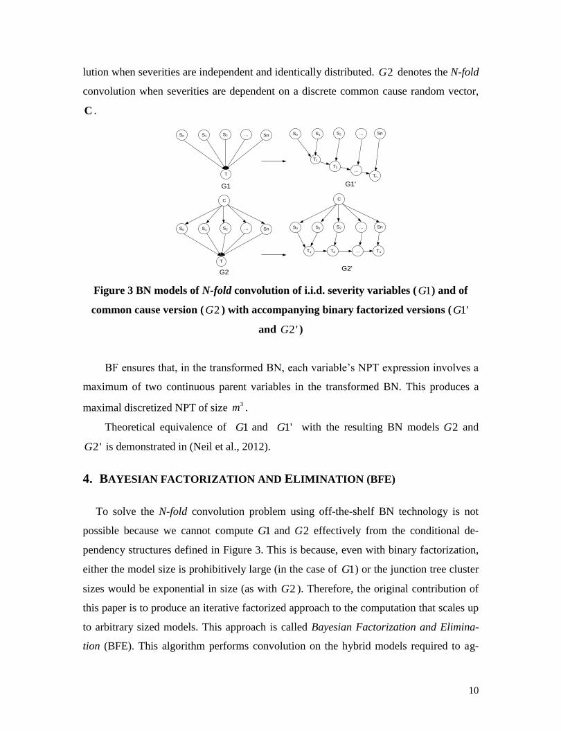
1'G and 2'G respectively as shown in Figure 3. In Figure 2 1G shows the N-fold convo-

10

lution when severities are independent and identically distributed. 2G denotes the N-fold

convolution when severities are dependent on a discrete common cause random vector,

C .

S0 S2S1

T

... Sn S0 S2S1

T1

... Sn

T2

Tn

...

G1 G1'

S0 S2S1

T

... Sn S0 S2S1

T1

... Sn

T2 Tn...

G2G2'

C C

Figure 3 BN models of N-fold convolution of i.i.d. severity variables ( 1G ) and of

common cause version ( 2G ) with accompanying binary factorized versions ( 1'G

and 2'G )

BF ensures that, in the transformed BN, each variable’s NPT expression involves a

maximum of two continuous parent variables in the transformed BN. This produces a

maximal discretized NPT of size 3m .

Theoretical equivalence of 1G and 1'G with the resulting BN models 2G and

2'G is demonstrated in (Neil et al., 2012).

4. BAYESIAN FACTORIZATION AND ELIMINATION (BFE)

To solve the N-fold convolution problem using off-the-shelf BN technology is not

possible because we cannot compute 1G and 2G effectively from the conditional de-

pendency structures defined in Figure 3. This is because, even with binary factorization,

either the model size is prohibitively large (in the case of 1G ) or the junction tree cluster

sizes would be exponential in size (as with 2G ). Therefore, the original contribution of

this paper is to produce an iterative factorized approach to the computation that scales up

to arbitrary sized models. This approach is called Bayesian Factorization and Elimina-

tion (BFE). This algorithm performs convolution on the hybrid models required to ag-

11

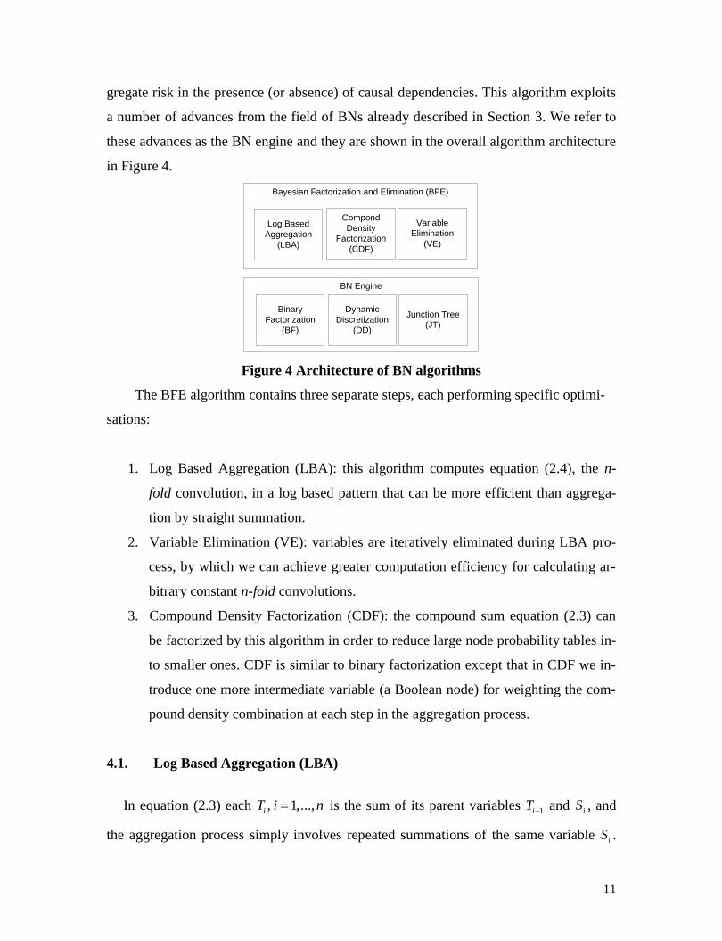
gregate risk in the presence (or absence) of causal dependencies. This algorithm exploits

a number of advances from the field of BNs already described in Section 3. We refer to

these advances as the BN engine and they are shown in the overall algorithm architecture

in Figure 4.

Bayesian Factorization and Elimination (BFE)

BN Engine

Log Based

Aggregation

(LBA)

Binary

Factorization

(BF)

Compond

Density

Factorization

(CDF)

Variable

Elimination

(VE)

Dynamic

Discretization

(DD)

Junction Tree

(JT)

Figure 4 Architecture of BN algorithms

The BFE algorithm contains three separate steps, each performing specific optimi-

sations:

1. Log Based Aggregation (LBA): this algorithm computes equation (2.4), the n-

fold convolution, in a log based pattern that can be more efficient than aggrega-

tion by straight summation.

2. Variable Elimination (VE): variables are iteratively eliminated during LBA pro-

cess, by which we can achieve greater computation efficiency for calculating ar-

bitrary constant n-fold convolutions.

3. Compound Density Factorization (CDF): the compound sum equation (2.3) can

be factorized by this algorithm in order to reduce large node probability tables in-

to smaller ones. CDF is similar to binary factorization except that in CDF we in-

troduce one more intermediate variable (a Boolean node) for weighting the com-

pound density combination at each step in the aggregation process.

4.1. Log Based Aggregation (LBA)

In equation (2.3) each , 1,...,iT i n is the sum of its parent variables 1iT and iS , and

the aggregation process simply involves repeated summations of the same variable iS .

12

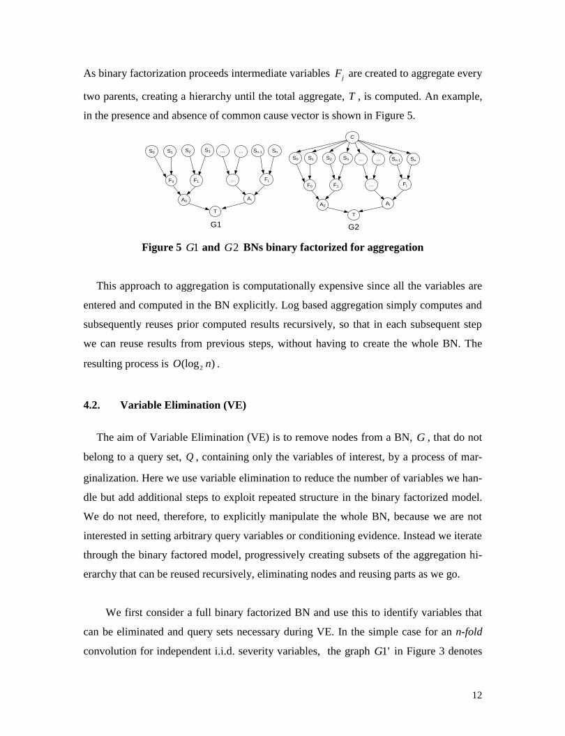
As binary factorization proceeds intermediate variables jF are created to aggregate every

two parents, creating a hierarchy until the total aggregate, T , is computed. An example,

in the presence and absence of common cause vector is shown in Figure 5.

G1 G2

T

AiA0

S2 S3

F1

S0 S1

F0

...

...

... Sn

Fj

Sn-1

S0

T

AiA0

S2 S3

F1

S1

F0

...

...

... Sn

Fj

Sn-1

C

Figure 5 1G and 2G BNs binary factorized for aggregation

This approach to aggregation is computationally expensive since all the variables are

entered and computed in the BN explicitly. Log based aggregation simply computes and

subsequently reuses prior computed results recursively, so that in each subsequent step

we can reuse results from previous steps, without having to create the whole BN. The

resulting process is 2(log )O n .

4.2. Variable Elimination (VE)

The aim of Variable Elimination (VE) is to remove nodes from a BN, G , that do not

belong to a query set, Q , containing only the variables of interest, by a process of mar-

ginalization. Here we use variable elimination to reduce the number of variables we han-

dle but add additional steps to exploit repeated structure in the binary factorized model.

We do not need, therefore, to explicitly manipulate the whole BN, because we are not

interested in setting arbitrary query variables or conditioning evidence. Instead we iterate

through the binary factored model, progressively creating subsets of the aggregation hi-

erarchy that can be reused recursively, eliminating nodes and reusing parts as we go.

We first consider a full binary factorized BN and use this to identify variables that

can be eliminated and query sets necessary during VE. In the simple case for an n-fold

convolution for independent i.i.d. severity variables, the graph 1'G in Figure 3 denotes

13

the binary factorized form of the computation of 0

n

n j

j

T S

after introducing the inter-

mediate binary factored variables 1 2 1{ , ,..., }nT T T . The marginal distribution for nT has the

form:

0 1 1

0 1 1

0 1 1 2 1

( ..., , ,..., )

1 1 2 1 1 0 1 0 1

( ..., , ,..., )

( ) ( , ,..., , , ,..., , )

( | , ) ( | , )... ( | , ) ( ) ( )... ( )

n n

n n

n n n n

S S T T

n n n n n n n

S S T T

P T P S S S T T T T

P T T S P T T S P T S S P S P S P S

(4.1)

(Exploiting the conditional independence relations in Figure 3)

Notice that every pair of parent variables iT and 1iS is independent in this model

and we can marginalize out each pair of iT and 1iS from the model separately. Equation

(4.1) can be alternatively expressed as predefined ‘query blocks’:

1 1 2 0 1

1 2 1 2 1 0 1 0 1 2

, , ,

( ) ( | , ) ... ( | , ) ( | , ) ( ) ( ) ( ) ... ( )n n

n n n n n

T S T S S S

P T P T T S P T T S P T S S P S P S P S P S

(4.2)

So, using (4.2) we can recursively marginalize out, i.e. eliminate or prune, each pair

of parents iT and 1iS from the model. For example, the elimination order in (4.2) could

be: 0 1 1 2 1{ , },{ , }...{ , }n nS S T S T S . The marginal distribution of nT , i.e. the final query set, is

then yielded at the last elimination step.

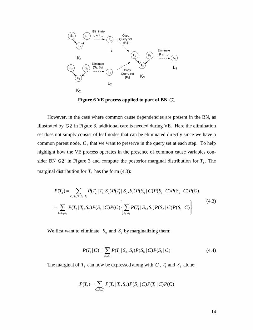
In order to illustrate the recursive BN graph operations, required during VE, consid-

er Figure 3 and BN 1G . The first few steps involved are shown in Figure 6. At each

stage we reuse the same graph structures and expressions for graphs 1 2 3{ , , }K K K and

1 2 3{ , , }L L L . We can proceed through the binary factorized BN, computing the marginal

distributions for the query set, removing elimination sets and repeating the process until

we exhaust the variable list.

14

S0 S1

F0

F0

Eliminate

{S0, S1}

F0 F1

A0

Eliminate

{F0, F1}

A0K1

L1

K3

L3

Copy

Query set

{F0}

S2 S3

F1

F1

Eliminate

{S2, S3}

K2

L2

Copy

Query set

{F1}

Figure 6 VE process applied to part of BN 1G

However, in the case where common cause dependencies are present in the BN, as

illustrated by 2G in Figure 3, additional care is needed during VE. Here the elimination

set does not simply consist of leaf nodes that can be eliminated directly since we have a

common parent node, C , that we want to preserve in the query set at each step. To help

highlight how the VE process operates in the presence of common cause variables con-

sider BN 2'G in Figure 3 and compute the posterior marginal distribution for 2T . The

marginal distribution for 2T has the form (4.3):

0 1 2 1

2 1 0 1

2 2 1 2 1 0 1 0 1 2

, , , ,

2 1 2 2 1 0 1 0 1

, , ,

( ) ( | , ) ( | , ) ( | ) ( | ) ( | ) ( )

( | , ) ( | ) ( ) ( | , ) ( | ) ( | )

C S S S T

C S T S S

P T P T T S P T S S P S C P S C P S C P C

P T T S P S C P C P T S S P S C P S C

(4.3)

We first want to eliminate 0S and 1S by marginalizing them:

0 1

1 1 0 1 0 1

,

( | ) ( | , ) ( | ) ( | )S S

P T C P T S S P S C P S C (4.4)

The marginal of 2T can now be expressed along with C , 1T and 3S alone:

2 1

2 2 1 2 2 1

, ,

( ) ( | , ) ( | ) ( | ) ( )C S T

P T P T T S P S C P T C P C

15

Next we eliminate 2S and 1T :

1 2

2 2 1 2 2 1

,

( | ) ( | , ) ( | ) ( | )T S

P T C P T T S P S C P T C (4.5)

In general, by variable elimination, we obtain the conditional distribution for each

variable 1nT (the sum of n severity variables) with the form:

2 1

1 1 2 1 2 1

,

( | ) ( | , ) ( | ) ( | )n n

n n n n n n

T S

P T C P T T S P T C P S C

(4.6)

Since (4.6) specifies the conditional distribution for variable 1 |nT C , and therefore

the posterior marginal distribution for the target n-fold convolution 1nT , the aggregate

total, is obtained by marginalizing out C .

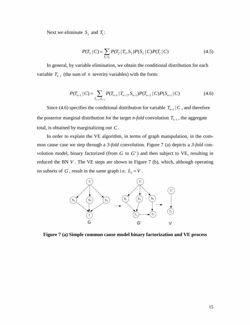
In order to explain the VE algorithm, in terms of graph manipulation, in the com-

mon cause case we step through a 3-fold convolution. Figure 7 (a) depicts a 3-fold con-

volution model, binary factorized (from G to 'G ) and then subject to VE, resulting in

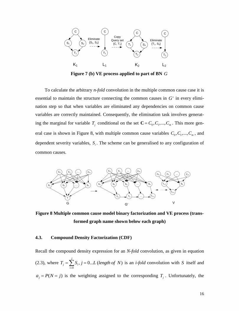
reduced the BN V . The VE steps are shown in Figure 7 (b), which, although operating

on subsets of G , result in the same graph i.e. 2L V .

S1 S2

C

T1

S3

T2

S1 S3S2

C

T

G G’ V

C

T2

Figure 7 (a) Simple common cause model binary factorization and VE process

16

S1 S2

C

T1

C

T1

Eliminate

{S1, S2}T1 S3

C

T2

Eliminate

{T1, S3}

C

T2

K1 L1 K2 L2

Copy

Query set

{C, T1}

Figure 7 (b) VE process applied to part of BN G

To calculate the arbitrary n-fold convolution in the multiple common cause case it is

essential to maintain the structure connecting the common causes in 'G in every elimi-

nation step so that when variables are eliminated any dependencies on common cause

variables are correctly maintained. Consequently, the elimination task involves generat-

ing the marginal for variable jT conditional on the set 0 1, ,..., mC C CC . This more gen-

eral case is shown in Figure 8, with multiple common cause variables 0 1, ,..., mC C C , and

dependent severity variables, iS . The scheme can be generalised to any configuration of

common causes.

S1

C1

S2

T2

C0

S3

T1

... Cm

...

...

Sn

Tn-1

C1C0 ... Cm

Sn

Tn-1

Tn-2S1

C1

S2 Sn

C0

...

T

... Cm

G VG’

...

Figure 8 Multiple common cause model binary factorization and VE process (trans-

formed graph name shown below each graph)

4.3. Compound Density Factorization (CDF)

Recall the compound density expression for an N-fold convolution, as given in equation

(2.3), where 0

, 0... ( )j

j i

i

T S j L length of N

is an i-fold convolution with S itself and

( )ja P N j is the weighting assigned to the corresponding jT . Unfortunately, the

17

compound density expression for ( )P T is very space inefficient and to address this we

need to factorize it. Given each component in the mixture is mutually exclusive, i.e. for a

given value of N the aggregate total is equal to one, and only one iT , variable, this fac-

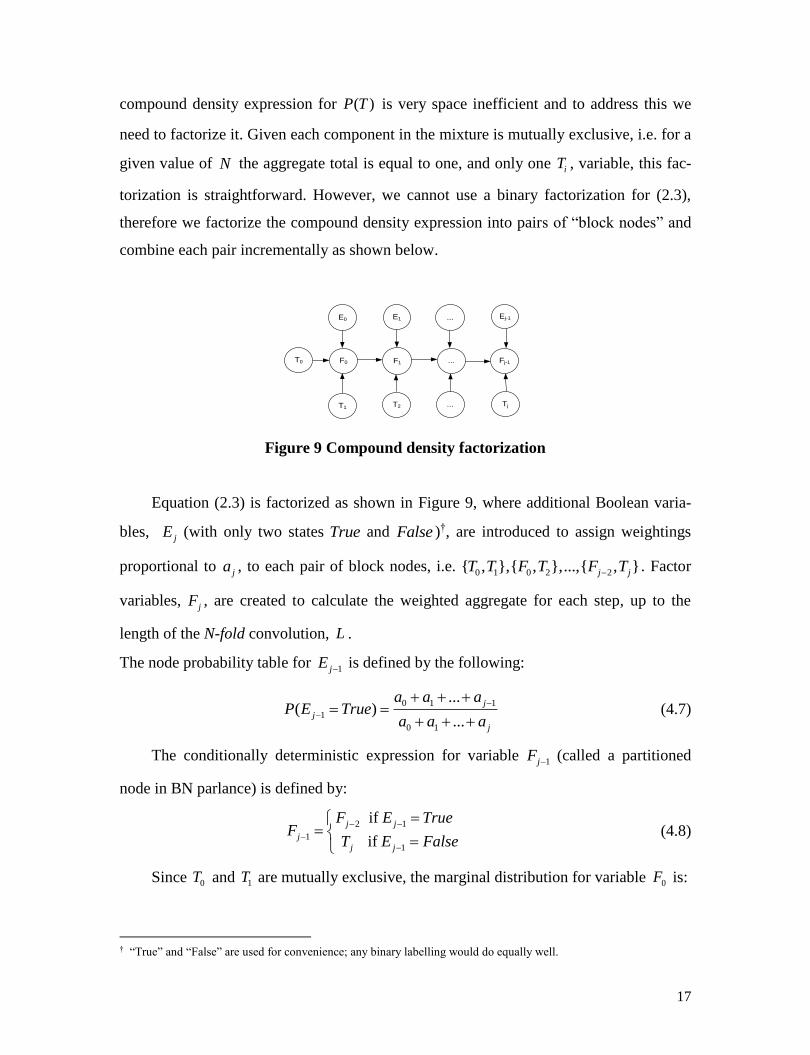
torization is straightforward. However, we cannot use a binary factorization for (2.3),

therefore we factorize the compound density expression into pairs of “block nodes” and

combine each pair incrementally as shown below.

F0

E0 E1

F1

...

...

... Fj-1

Ej-1

T0

T1 T2 Tj

Figure 9 Compound density factorization

Equation (2.3) is factorized as shown in Figure 9, where additional Boolean varia-

bles, jE (with only two states True and False )†, are introduced to assign weightings

proportional to ja , to each pair of block nodes, i.e.

0 1 0 2 2{ , },{ , },...,{ , }j jT T F T F T. Factor

variables, jF , are created to calculate the weighted aggregate for each step, up to the

length of the N-fold convolution, L .

The node probability table for 1jE is defined by the following:

0 1 1

1

0 1

...( )

...

j

j

j

a a aP E True

a a a

(4.7)

The conditionally deterministic expression for variable 1jF (called a partitioned

node in BN parlance) is defined by:

2 1

1

1

if

if

j j

j

j j

F E TrueF

T E False

(4.8)

Since 0T and 1T are mutually exclusive, the marginal distribution for variable 0F is:

† “True” and “False” are used for convenience; any binary labelling would do equally well.

18

0 0 0 0 1 0 0 1 1( ) ( ) ( ) ( ) ( ) ( )F P E True P T P E False P T a P T a P T

which is identical to the first two terms in the original compound density expres-

sion, (2.3). Similarly, the marginal for variable jF becomes:

1 1 2 1( ) ( ) ( ) ( )j j j j jF P E True P F P E False P T (4.9)

After applying the CDF method to (2.3) we have the marginal for 1jF as shown by

(4.9), which yields the compound density, ( )P T , for the N-fold convolution. Therefore

by using the CDF method we can compute the compound density (2.3) more efficiently.

The CDF method is a general way of factorizing a compound density. It takes as in-

put any n-fold convolution, regardless of the causal structure governing the severity vari-

ables. Note that the CDF method can be made more efficient by applying variable elimi-

nation (VE) to remove leaf nodes. Likewise we can execute the algorithm recursively

reuse the same BN fragment ( | , , )P F F T E .

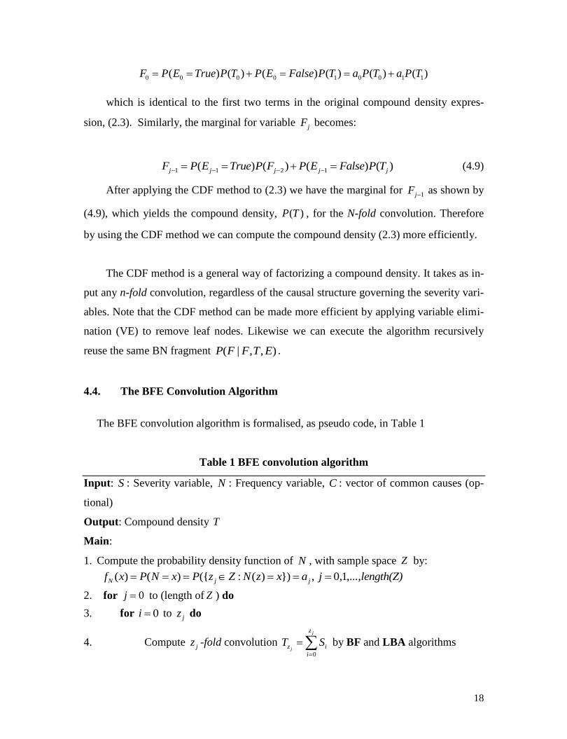
4.4. The BFE Convolution Algorithm

The BFE convolution algorithm is formalised, as pseudo code, in Table 1

Table 1 BFE convolution algorithm

Input: S : Severity variable, N : Frequency variable, C : vector of common causes (op-

tional)

Output: Compound density T

Main:

1. Compute the probability density function of N , with sample space Z by:

( ) ( ) ({ : ( ) }) , 0 1N j jf x P N x P z Z N z x a j , ,...,length(Z)

2. for 0j to (length of Z ) do

3. for 0i to jz do

4. Compute jz -fold convolution 0

j

j

z

z i

i

T S

by BF and LBA algorithms

19

5. Eliminate nodes (out of query set) by VE algorithm

6. end for

7. While 2j do

8. Apply CDF algorithm to factorize (2.3) by probability density of N

Compute 1 1 2 1( ) ( ) ( ) ( )jj j j j zF P E True P F P E False P T

9. Eliminate nodes iS , 2jF and

jzT by VE algorithm

10. end while

11. end for

12. return 1( )jP F

{marginal distribution of T }

5. DECONVOLUTION USING THE BFE ALGORITHM

5.1. Deconvolution

Where we are interested in the posterior marginal distribution of the causal variables

conditional on the convolution aggregated results we can perform deconvolution, in ef-

fect reversing the direction of inference involved in convolution. This is of interest in

sensitivity analysis, where we might be interested in identifying which causal variables

have the largest, differential, impact on some summary statistic of the aggregated total,

such as the mean loss or the conditional Value At Risk (cVAR), derived from

0( | )P C T t .

One established solution for deconvolution involves inverse filtering using Fourier

Transforms, whereby the severity, S , is obtained by inverse transformation from its

characteristic function. Alternative analytical estimation methods, i.e. maximum likeli-

hood, and numerical evaluation involving Fourier transforms or simulation based sam-

pling methods, can be attempted but none of them is known to have been applied to N-

fold deconvolution in hybrid models containing discrete causal variables.

BN based inference offers an alternative, natural, way of solving deconvolution be-

cause it offers both predictive (cause to consequence) reasoning and diagnostic (conse-

quence to cause) reasoning. This process of backwards inference is called “back propa-

gation”, whereby evidence is entered into the BN on a consequence node and then the

20

model is updated to determine the posterior probabilities of all parent and antecedent var-

iables in the model. A “backwards” version of the BFE algorithm offers a solution for

answering deconvolution problems, in a general way without making any assumptions

about the form of the density function of S . The approach again uses a discretized form

for all continuous variables in the hybrid BN, thus ensuring that the frequency distribu-

tion, N , is identifiable.

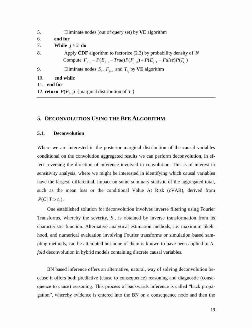
EXAMPLE 1

Consider a simple BN with parent variable distributions

2~ ( 5, 5)X Normal , 2~ ( 10, 10)Y Normal and likelihood function for a

child variable ( | , ) ( )P Z X Y P Z X Y . Figure 12(a) show the prior convolution ef-

fects of the back propagation calculation, as marginal distributions superimposed on the

BN graph. The exact posterior marginal for Z is 2~ ( 15, 15)Z Normal . Our ap-

proximation produces a mean of 14.99 and variance 16.28.

(a) (b)

Figure 12 (a) Convolution and (b) Deconvolution

If we set an observation 0Z z and perform inference we obtain the posterior mar-

ginal of X by Bayes’ rule:

0

00

0 0

,

( | , ) ( ) ( )( , )

( | )( ) ( | , ) ( ) ( )

Y

X Y

P Z z X Y P X P YP X Z z

P X Z zP Z z P Z z X Y P X P Y

(5.1)

21

Where our likelihood ( | , )P Z X Y is a convolution function, equation (5.1) defines

the deconvolution and yields the posterior marginal distribution of X given observation

0Z z . In Figure 12(b), the observation is 30Z (which is approximated as a discrete

bin of given width), and the posterior for X has updated to a marginal distribution with

mean 9.97 and variance 3.477.

In the example shown in Figure 12 the parent variables X and Y are conditionally

dependent given the observation 0Z z . For n-fold convolution with or without common

causes an observation on the iT variables would also make each of the severity variables

dependent and we can perform n-fold deconvolution using the DD and JT alone for small

models containing non i.i.d severity variables with query block sizes of maximum cardi-

nality four. For large models, containing i.i.d severity variables BFE provides a correct

solution with minimal computational overhead.

T0 TT1

N

C

T

T2

C

N

A

S0 S2S1

C

T

G’

T0 T1 T2

G

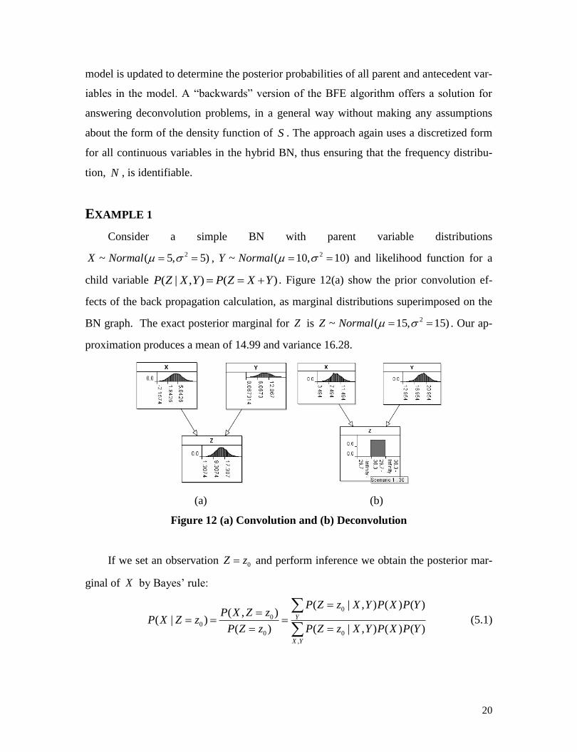
Figure 13 Binary factored common cause N-fold BN, A , reduced by applying the

VE algorithm to G and then 'G

We have already noted that during N-fold convolution the iT variables are mutually

exclusive, such that for a given N i , if the variable iT exists, then the other variables

do not. This fact can be exploited during factorization during the deconvolution process-

es.

Consider the common cause BN model shown in Figure 13. The fully specified

model is shown in BN graph A . The posterior distributions for all nodes can be comput-

ed by way of the BFE convolution algorithm and we can cache any distributions and pa-

rameters we might need during this process, for subsequent use during deconvolution.

The BFE deconvolution algorithm then proceeds by eliminating all intermediate, fre-

22

quency and severity variables until we get the reduced BN graph containing the final

query set of interest.

Let us assume the model structure in BN A of Figure 13. Here frequency, N , is

discretized into three finite states {1, 2, 3}, so there are three n-fold convolution variables

0

, 0,1,2i

i j

j

T S i

each corresponding to the sum of one, two and three severity varia-

bles. T is the compound distribution defined by:

0 0 1 1 2 2( ) ( ) ( ), ( ), 0,1,2iT a P T a P T a P T a P N i i

Given evidence 0T t the deconvolution of C is achieved by:

00

0

0

, ,

( , )( | )

( )

( | ( )) ( ) ( | ( )) ( | ) ( )i i

i i i

S T N

P C T tP C T t

P T t

P T t pa T P N P T pa T P S C P C

(5.2)

where ( )pa T denotes the parents of T . So, once the convolution model has

eliminated all irrelevant variables, in this case , , ,ji z j jS T E F we would be left with the

query set, which here is { , }Q C T .

5.2. Reconstructing the frequency variables during deconvolution

If we are also interested in including the frequency variable, N , in our query set we

must be careful to cache variables jE ,

2jF and

jzT during convolution. Recall that the

prior distribution for N was decomposed into the jE during compound density factori-

zation, therefore we need some way of updating this prior using the new posterior proba-

bilities generated on the Boolean variables, jE , during deconvolution. To perform de-

convolution on N it is first necessarily to reconstruct N from the jE variables that to-

gether composed the original N .

23

Reconstruction involves composing all Boolean variables, jE , into the frequency

variable N , in a way that the updating of jE can directly result in generating a new pos-

terior distribution of N . The model is established by connecting all jE nodes to N ,

where the new NPT for N has the form of combining all its parents. However, it turns

out this NPT is exponential ( 12 j ) in size. To avoid the drawback we use an alternative,

factorized, approach that can reconstruct the NPT incrementally.

As before, we reconstruct N using binary factorization where the conditioning is

conducted efficiently using incremental steps. Here the intermediate variables produced

during binary factorization, , ( 0,..., 1)kN k j , are created efficiently by ensuring their

NPTs are of minimal size.

The routine for constructing the NPTs for , ( 0,..., 1)kN k j from the jE ’s is:

1. Order parents jE and

1jE from higher index to lower index for kN ’s NPT

(since jE is Boolean variable with only two states, one concatenating all

1jE ’s

states and another state is single state that 1jE does not contain. In this example

1E should be placed on top of 0E in the NPT table, as it is easier for comparing

the common sets)

2. As we have already generated the NPT map of jE ,

1jE and kN . Next we spec-

ify the NPT entry with unit value (“1”) at kN , when jE and

1jE has com-

mon sets (In this example, E.g. 1E and 0E have common sets "0" and

"1" )

3. Specify NPT entry with value (“1”) at kN , when jE and 1jE has no com-

mon sets and jE (

jE has one state that 1jE does not contain, so under

this case kN only needs to be consistent with jE as the changes on

1jE won’t

affect the probability ( )kP N , E.g. in this example it is when 1 "2"E )

4. Specify NPT entry with value (“0”) at all other entries.

24

We repeat this routine for all , ( 0,..., 1)kN k j until we have exhausted all jE ’s,

producing a fully reconstructed N . Once we have built the reconstructed structure ( kN )

for N , in fact the updates of jE ’s probabilities are directly mapped to kN , and so de-

convolution of N is retrieved.

5.3. The BFE Deconvolution Algorithm with examples

The BFE deconvolution algorithm, for N-fold deconvolution, is formalised, as pseudo

code, in Table 2:

Table 2 BFE deconvolution algorithm

Input: S : Severity variable, N : Frequency variable, C : vector of common causes and

0T t

Output: posterior marginal of query set members i.e. 0( | )P T tC , 0( | )P N T t

Main:

1. do convolution BFE algorithm to produce final query set

2. if N is in query set

3. reconstruct N from jE

4. end if

5. set evidence 0t on T and perform inference

6. return posterior marginal distributions for query set

EXAMPLE 2

Consider a simplified example for deconvoluting N , suppose frequency distribu-

tion N is discretized as {0.1, 0.2, 0.3, 0.4} with discrete states {0,1, 2, 3} and

~ (1)S Exponential . Figure 14 (a) shows these incremental steps for example 4. In this

example there are three parents ( 0 1 2, ,E E E ) to N . The incremental composition steps of

jE have introduced two intermediate variables 0N and 1N , and we expect the frequency

25

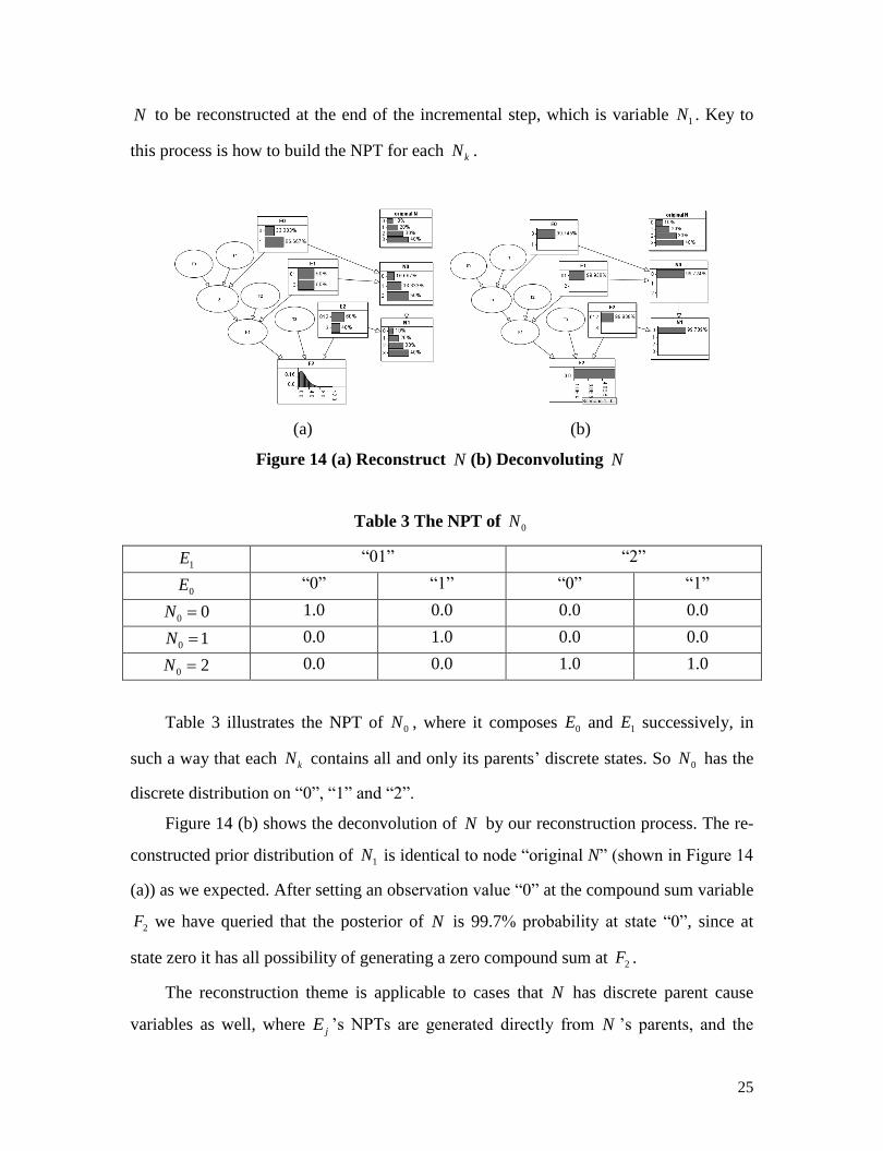
N to be reconstructed at the end of the incremental step, which is variable 1N . Key to

this process is how to build the NPT for each kN .

(a) (b)

Figure 14 (a) Reconstruct N (b) Deconvoluting N

Table 3 The NPT of 0N

1E “01” “2”

0E “0” “1” “0” “1”

0 0N 1.0 0.0 0.0 0.0

0 1N 0.0 1.0 0.0 0.0

0 2N 0.0 0.0 1.0 1.0

Table 3 illustrates the NPT of 0N , where it composes 0E and 1E successively, in

such a way that each kN contains all and only its parents’ discrete states. So 0N has the

discrete distribution on “0”, “1” and “2”.

Figure 14 (b) shows the deconvolution of N by our reconstruction process. The re-

constructed prior distribution of 1N is identical to node “original N” (shown in Figure 14

(a)) as we expected. After setting an observation value “0” at the compound sum variable

2F we have queried that the posterior of N is 99.7% probability at state “0”, since at

state zero it has all possibility of generating a zero compound sum at 2F .

The reconstruction theme is applicable to cases that N has discrete parent cause

variables as well, where jE ’s NPTs are generated directly from N ’s parents, and the

26

deconvolution is performed by BFE deconvolution algorithm. Experiment 3 in section 6

considers deconvoluting common cause variables where the model has this form.

6. EXPERIMENTS

We report on a number of experiments using the BFE algorithm in order to determine

whether it can be applied to a spectrum of risk aggregation problem archetypes. Where

possible the results are compared to analytical results, FFT, Panjer’s approach and Monte

Carlo simulation. The following experiments, with accompanying rationale, were carried

out:

1. Experiment 1: Convolution with multi-modal (mixtures of) severity distribution.

We believe this to be a particularly difficult case for those methods that are more

reliant on particular analytical assumptions. Practically, multi-modal distributions

are of interest in cases where we might have extreme outcomes, such as sharp re-

gime shifts in asset valuations.

2. Experiment 2: Convolution with discrete common causes variables. This is the

key experiment in the paper since these causes will be co-dependent and the se-

verity distribution will depend on their values (and hence will be a conditional

mixture).

3. Experiment 3: Deconvolution with discrete common causes. This is the inverse of

experiment 2 where we seek to estimate the posterior marginal for the common

causes conditioned on some observed total aggregated value.

The computing environment settings for the experiments are as follows. Operation

system: Windows XP Professional, Intel i5 @ 3.30GHz, 4.0GB RAM. AgenaRisk was

used to implement the BFE algorithm, which was written in java, where typically the DD

settings were for 65 iterations for severity variables and 25 iterations for the frequency

variable. A sample size of 2.0E+5 was used as the settings in R(R, 2013) for the Monte

Carlo simulation.

6.1. Experiment 1: Convolution with multi-modal severity distribution

27

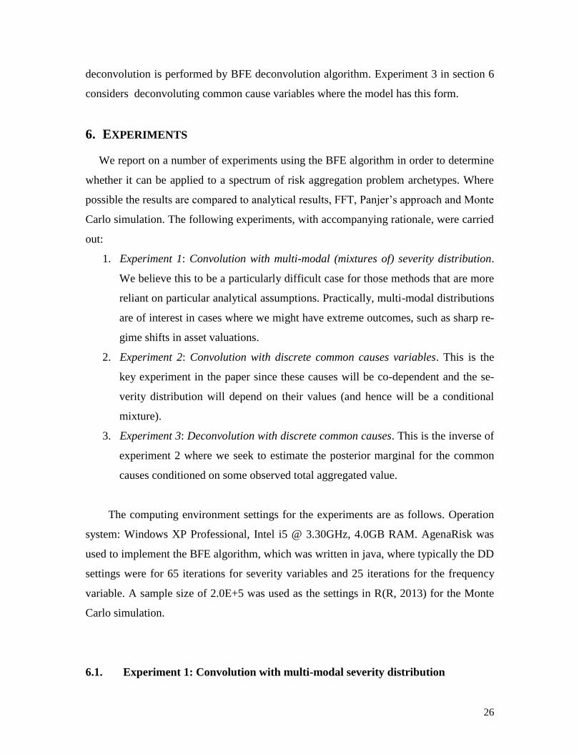
Here we set the event frequency as ~ (50)N Poisson but the severity distribution is a

mixture distribution, ~ SS f :

(0.2) (5,1.5) (0.3) (25, 2) (0.4) (50, 3) (0.1) (100, 2)Sf Gamma Normal Normal Gamma

In a hybrid BN a mixture distribution is modelled by conditioning the severity varia-

ble on one or more partitioning discrete variables, C . Assuming that that severity varia-

bles, jS , are i.i.d. we can calculate the compound density using BFE.

The characteristic function of a mixture distribution is inconvenient to define (with

continuous and discrete components). The analytical and programming effort needed to

solve each multi-modal severity distribution for Panjer is high, so here we compare with

MC only.

Table 6 Results of convolution with multi-modal severity distribution

Algorithm Mean Standard

Deviation

95th

Percentile

99th

Percentile

Analysis

Effort

MC 2444.8 516.7 3340.0 3787.7 Low

BFE 2441.1 523.3 3341.5 3783.1 Low

The corresponding marginal distribution for the query node set { , , }T N S is shown

in Figure 18.

28

Figure 19 Marginal distributions for overlaid on BN graph containing query nodes

for Experiment 1

6.2. Experiment 2: Convolution with discrete common causes variables

Loss distributions from operational risk can vary in different circumstances, e.g. ex-

hibiting co-dependences among causes. Suppose in some cases that losses are caused by

daily operations and these losses are drawn from a mixture of truncated Normal distribu-

tions, whereas extreme or some unexpected losses are distributed in a more severe distri-

bution. We model this behaviour by a hierarchical common cause combination 0 4,...,C C .

The severity variable S is conditioning on common cause variable, 0 1 2, ,C C C . And

these common cause variables are conditioned on higher common causes 3C and 4C .

Severity NPT is shown in Table 7. The frequency distribution of losses is modelled as

~ (50)N Poisson .

Table 7 Severity NPT

0C High Low

1C High Low High Low

2C High Low High Low High Low High Low

Expression Normal

(1,2)

Normal

(2,3)

Normal

(3,4)

Normal

(4,5)

Normal

(100,110)

Normal

(110,120)

Normal

(120,130)

Normal

(130,140)

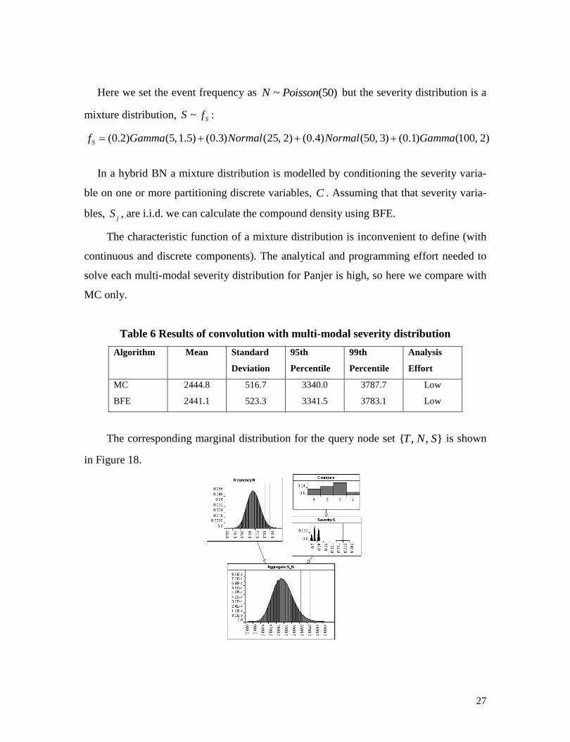
(a) (b)

Figure 20 (a) Common cause dependent severity; (b) 16-fold convolution of depend-

ent severity

29

In Figure 20 (a) the model severities with dependencies by common cause variables

0 4,...,C C is introduced. Figure 20 (b) depicts a 16-fold convolution of dependent severi-

ties using the variable elimination method. For any given frequency distribution, N , we

can apply the BFE convolution algorithm to calculate the common cause N-fold convolu-

tion.

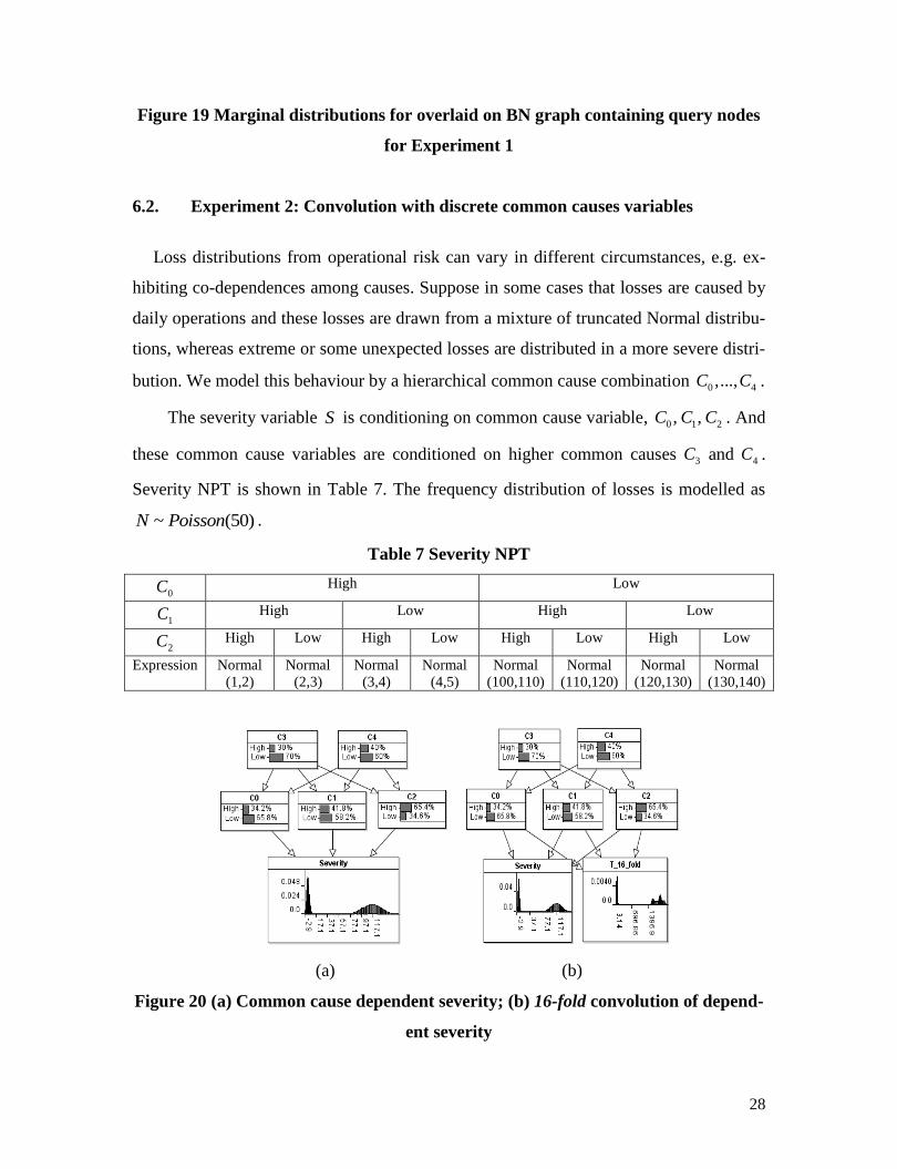
(a) (b)

Figure 21 Compound densities (a) MC; (b) BFE

Table 8 Common cause N-fold convolution density

Algorithm Mean Median Standard

Deviation

95th

Percentile

99th

Percentile

MC 3831 5017 2784 7215 8023

BFE 3871 5052 3255 7267 8115

Figure 21 illustrates the output compound densities for the compared algorithms.

Table 8 shows the results for the two approaches are almost identical on summary statis-

tics except the small difference on standard deviation. BFE has offered a unified ap-

proach to construct and compute such a model conveniently.

6.3. Experiment 3: deconvolution with discrete common causes variables

30

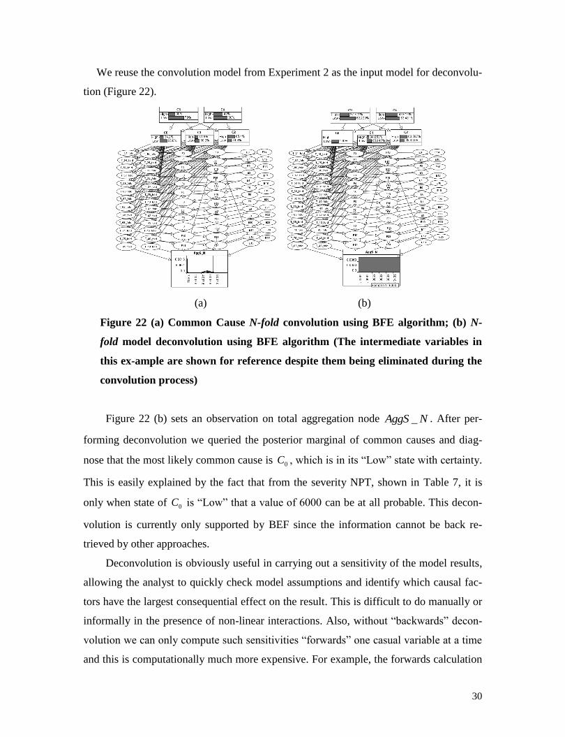
We reuse the convolution model from Experiment 2 as the input model for deconvolu-

tion (Figure 22).

(a) (b)

Figure 22 (a) Common Cause N-fold convolution using BFE algorithm; (b) N-

fold model deconvolution using BFE algorithm (The intermediate variables in

this ex-ample are shown for reference despite them being eliminated during the

convolution process)

Figure 22 (b) sets an observation on total aggregation node _AggS N . After per-

forming deconvolution we queried the posterior marginal of common causes and diag-

nose that the most likely common cause is 0C , which is in its “Low” state with certainty.

This is easily explained by the fact that from the severity NPT, shown in Table 7, it is

only when state of 0C is “Low” that a value of 6000 can be at all probable. This decon-

volution is currently only supported by BEF since the information cannot be back re-

trieved by other approaches.

Deconvolution is obviously useful in carrying out a sensitivity of the model results,

allowing the analyst to quickly check model assumptions and identify which causal fac-

tors have the largest consequential effect on the result. This is difficult to do manually or

informally in the presence of non-linear interactions. Also, without “backwards” decon-

volution we can only compute such sensitivities “forwards” one casual variable at a time

and this is computationally much more expensive. For example, the forwards calculation

31

of T from ten Boolean common cause variables would require 102 calculations versus 40

in the backwards case (assuming T was discretized into 40 states).

7. CONCLUSION AND FUTURE WORK

This paper has reviewed historical, popular, methods for performing risk aggregation

and compared them with a new method called Bayesian Factorization and Elimination

(BFE). The method exploits a number of advances from the field of Bayesian Networks,

covering methods to approximate statistical and conditionally deterministic functions and

to factorize multivariate distributions for efficient computation. Our objective for BFE

was for it to perform aggregation for classes of problems that the existing methods can-

not solve (namely hybrid situations involving common causes) while performing at least

as well on conventional aggregation problems. Our experiments show that our objectives

were achieved. For more difficult hybrid problems the experimental results show that

BFE provides a more general solution that is not possible with the previous methods.

Additionally, the BFE approach can be easily extended to perform deconvolution

for the purposes of stress testing and sensitivity analysis in a way that competing meth-

ods cannot currently offer. The BFE deconvolution method reported here provides a low

resolution result, which is likely good enough for the purposes of model checking and

sensitivity analysis. However, we are investigating an alternative high resolution ap-

proach whereby variables are discretized efficiently during the deconvolution process,

thus providing more accurate posterior results.

On-going and future research is also focused on more complex situations involving

both copulas and common cause variables. The challenge here is to decompose these

models into lower dimensional joint distributions, where complexity can be further re-

duced by factorization. One final area of interest includes optimization of the results such

that we might choose a set of actions in the model that maximize returns for minimum

risk: we see deconvolution playing a strong role here.

32

Acknowledgements

We are grateful to the editor as well as the anonymous reviewers for comments and sug-

gestions on the paper.

References

AgenaRisk. (2014). AgenaRisk. Retrieved December 23, 2014, from

http://www.agenarisk.com/

Arbenz, P., & Canestraro, D. (2012). Estimating Copulas for Insurance from Scarce Ob-

servations, Expert Opinion and Prior Information: A Bayesian Approach. ASTIN

Bulletin, 42(01), 271–290. doi:10.2143/AST.42.1.2160743

Black, F., & Litterman, R. B. (1991). Asset Allocation: Combining Investor Views with

Market Equilibrium. The Journal of Fixed Income, 1(2), 7–18.

doi:10.3905/jfi.1991.408013

Brechmann, E. C. (2014). Hierarchical Kendall copulas: Properties and inference. Cana-

dian Journal of Statistics. doi:10.1002/cjs.11204

Bruneton, J.-P. (2011). Copula-based Hierarchical Aggregation of Correlated Risks. The

behaviour of the diversification benefit in Gaussian and Lognormal Trees.

arXiv:1111.1113 [q-Fin]. Retrieved from http://arxiv.org/abs/1111.1113

Cooper, G. F., & Herskovits, E. (1992). A Bayesian method for the induction of proba-

bilistic networks from data. Machine Learning, 9(4), 309–347.

doi:10.1007/BF00994110

33

Cowell, R. G., Verrall, R. J., & Yoon, Y. K. (2007). Modeling Operational Risk With

Bayesian Networks. Journal of Risk and Insurance, 74(4), 795–827.

doi:10.1111/j.1539-6975.2007.00235.x

Embrechts, P. (2009). Copulas: A Personal View. Journal of Risk and Insurance, 76(3),

639–650. doi:10.1111/j.1539-6975.2009.01310.x

Fenton, N., & Neil, M. (2012). Risk Assessment and Decision Analysis with Bayesian

Networks. CRC Press.

Grubel, R., & Hermesmeier, R. (1999). Computation of compound distributions I: Alias-

ing errors and exponential tilting. ASTIN Bulletin, 2(29), 197–214.

Heckman, P. E., & Meyers, G. G. (1983). The calculation of aggregate loss distributions

(pp. 22–61). Presented at the Proceedings of the Casualty Actuarial Society.

IMF. (2009). IMF Global Financial Stability Report -- Navigating the Financial Chal-

lenges Ahead.

Jensen, F. V., & Nielsen, T. D. (2009). Bayesian Networks and Decision Graphs.

Springer.

Kozlov, A. V., & Koller, D. (1997). Nonuniform Dynamic Discretization in Hybrid

Networks. In Proceedings of the Thirteenth Conference on Uncertainty in Artifi-

cial Intelligence (pp. 314–325). San Francisco, CA, USA: Morgan Kaufmann

Publishers Inc.

Laeven, L., & Valencia, F. (2008). Systemic Banking Crises: A New Database (SSRN

Scholarly Paper No. ID 1278435). Rochester, NY: Social Science Research Net-

work.

McNeil, A. J., Frey, R., & Embrechts, P. (2010). Quantitative Risk Management: Con-

cepts, Techniques, and Tools. Princeton University Press.

34

Meucci, A. (2008). Fully Flexible Views: Theory and Practice (SSRN Scholarly Paper

No. ID 1213325). Rochester, NY: Social Science Research Network.

Meyers, G. G. (1980). An Analysis of Retrospective Rating. In PCAS LXVII.

Neil, M., Chen, X., & Fenton, N. (2012). Optimizing the Calculation of Conditional

Probability Tables in Hybrid Bayesian Networks Using Binary Factorization.

IEEE Transactions on Knowledge and Data Engineering, 24(7), 1306–1312.

doi:10.1109/TKDE.2011.87

Neil, M., & Fenton, N. (2008). Using Bayesian networks to model the operational risk to

information technology infrastructure in financial institutions. Journal of Finan-

cial Transformation, 22, 131–138.

Neil, M., Tailor, M., & Marquez, D. (2007). Inference in hybrid Bayesian networks us-

ing dynamic discretization. Statistics and Computing, 17.

Nelsen, R. B. (2007). An Introduction to Copulas. Springer.

Panjer, H. H. (1981). Recursive evaluation of a family of compound distributions. ASTIN

Bulletin, 1(12), 22–26.

Pearl, J. (1993). [Bayesian Analysis in Expert Systems]: Comment: Graphical Models,

Causality and Intervention. Statistical Science, 8(3), 266–269.

Politou, D., & Giudici, P. (2009). Modelling Operational Risk Losses with Graphical

Models and Copula Functions. Methodology and Computing in Applied Probabil-

ity, 11(1), 65–93. doi:10.1007/s11009-008-9083-5

R. (2013). The R Project for Statistical Computing. Retrieved December 23, 2013, from

http://www.r-project.org/

Rebonato, R. (2010). Coherent Stress Testing: A Bayesian Approach to the Analysis of

Financial Stress. John Wiley & Sons.