rigid body dynamics simulation for robot motion planning - Infoscience

POUR L'OBTENTION DU GRADE DE DOCTEUR ÈS SCIENCES

PAR

ingénieur informaticien diplômé EPFde nationalité suisse et originaire de Kerns (OW)

acceptée sur proposition du jury:

Prof. A. Billard, présidente du juryProf. H. Bleuler, directeur de thèse

Prof. G. A. de Paula Caurin, rapporteurProf. D. Thalmann, rapporteur

Dr R. Vuillemin, rapporteur

rigid body dynamics simulation for robot motion planning

Alan ETTLIN

THÈSE NO 3663 (2006)

ÉCOLE POLYTECHNIQUE FÉDÉRALE DE LAUSANNE

PRÉSENTÉE LE 17 NOVEmBRE 2006

à LA FACULTÉ DES SCIENCES ET TECHNIQUES DE L'INGÉNIEUR

Laboratoire de systèmes robotiques 1

PROGRAmmE DOCTORAL EN SYSTÈmES DE PRODUCTION ET ROBOTIQUE

Suisse2006

ABSTRACT

The development of robot motion planning algorithms is inherently a challeng-ing task. This is more than ever true when the latest trends in motion planningare considered. Some motion planners can deal with kinematic and dynamic con-straints induced by the mechanical structure of the robot. Another class of motionplanners fulfill various types of optimality conditions, yet others include means ofdealing with uncertainty about the robot and its environment. Sensor-based motionplanners gather information typically afflicted with errors about a partially knownenvironment in order to plan a trajectory therein. In another research area it isinvestigated how multiple robots best cooperate to solve a common task.

In order to deal with the complexity of developing motion planning algorithms,it is proposed in this document to resort to a simulation environment. The advan-tages of doing so are outlined and a system named Ibex presented which is wellsuited to support motion planner development. The developed framework makesuse of rigid body dynamics algorithms as simulation kernel. Further, various com-ponents are included which integrate the simulation into existing engineering en-vironments. Simulation content can be conveniently developed through extensionsof well-established 3D modelling tools. The co-simulation with components fromother domains of physics is provided by the integration into a leading dynamic mod-elling environment. Robotic actuator models can be combined with a rigid bodydynamics simulation using this mechanism. The same configuration also allows toconveniently develop control algorithms for a rigid body dynamics setup and offerspowerful tools for handling and analysing simulation data. The developed simu-lation framework also offers physics-based models for simulating various sensors,most prominently a model for sensor types based on wave propagation, such aslaser range finding devices.

Application examples of the simulation framework are presented from the mo-bile robotics rough-terrain motion planning domain. Three novel rough-terrainplanning algorithms are presented which are extensions of known approaches. Toquantify the navigational difficulty on rough terrain, a new generic measure named“obstacleness” is proposed which forms the basis of the proposed algorithms.

The first algorithm is based on Randomised Potential Field Planners (RPP)and consequently is a local algorithm. The second proposed planner extends

ii

RRTconnect, a bi-directional Rapidly Exploring Random Tree (RRT) algorithm andbiases exploration of the search space towards easily traversable regions. The thirdplanner is an extension of the second approach and uses the same heuristic to grow aseries of additional local RRTs. This allows it to plan trajectories through complexdistributions of navigational difficulty benefitting from easy regions throughout themotion plan.

A complete example is shown in which the proposed algorithms form the basisfor sensor-based dynamic re-planning simulated in the presented framework. Inthe scenario, a simulated planetary rover navigates a long distance over rough ter-rain while gathering sensor data about the terrain topography. Where obstacles aresensed which interfere with the original motion plan, dynamic re-planning routinesare applied to circumnavigate the hindrances.

In the course of this document a complete simulation environment is presentedby means of a theoretical background and application examples which can signif-icantly support the development of robot motion planning algorithms. The frame-work is capable of simulating setups which fulfil the requirements posed by state-of-the-art motion planning algorithm development.

KEYWORDS

rigid body dynamics, robot motion planning, rough-terrain navigation,sensor simulation, simulation content tool-chain

ZUSAMMENFASSUNG

Die Entwicklung von Pfadplanungsalgorithmen fur Roboter ist an sich schon ei-ne schwierige Aufgabe. Dies ist erst recht wahr, wenn die neuesten Entwicklun-gen in der Pfadplanung berucksichtigt werden. Einige Pfadplaner konnen mit ki-nematischen und dynamische Einschrankungen umgehen, die von der mechani-schen Struktur des Roboters erzeugt werden. Eine andere Kategorie von Pfadpla-nern erfullt diverse Optimalitatskriterien, wieder andere Planer beinhalten Metho-den um mit Ungewissheiten uber den Roboter sowie dessen Umgebung umgehenzu konnen. Sensorbasierte Pfadplaner erfassen typischerweise fehlerbehaftete Da-ten uber eine teilweise bekannte Umgebung um darin eine Trajektorie zu errechnen.In einem anderen Forschungsfeld wird untersucht wie mehrere Roboter am Bestenmiteinander kooperieren konnen um eine gemeinsame Aufgabe zu erfullen.

Um die Komplexitat in der Entwicklung von Pfadplanungsalgorithmen besserhandhaben zu konnen wird in diesem Dokument vorgeschlagen auf eine Simu-lationsumgebung zuruckzugreifen. Die Vorteile eines solchen Vorgehens werdenerlautert und ein System namens Ibex vorgestellt, welches gut geeignet ist umdie Pfadplanungsalgorithmenentwicklung zu unterstutzen. Die entwickelte Simu-lationsumgebung verwendet Starrkorperdynamikalgorithmen als Simulationskern.Ferner sind weitere Komponenten entwickelt worden, welche die Simulation inbestehende Entwicklungsumgebungen integrieren. Das Erstellen von Simulations-inhalten wird mittels Erweiterungen von etablierten 3D Modellierungswerkzeugenermoglicht. Die Ko-simulation mit Komponenten aus anderen Gebieten der Physikwird durch die Integration in eine fuhrende Entwicklungsumgebung zum erstel-len dynamischer Modelle sichergestellt. Modelle von Robotik-Aktoren konnen aufdiese weise einfach mit einer Starrkorperdynamiksimulation kombiniert werden.Dieselbe Konfiguration bietet auch eine machtige Moglichkeit Regelalgorithmenfur einen Starrkorperdynamikaufbau zu entwickeln sowie die anfallenden Simula-tionsdaten zu handhaben und auszuwerten. Die entwickelte Simulationsumgebungbietet ebenfalls physikbasierte Modelle zur Simulation verschiedener Sensortypenan, z.B. ein Modell fur Sensoren welche auf Wellenausbreitung basieren, wie etwaein Laser-Distanzmessgerat.

Es werden Anwendungsbeispiele der Simulationsumgebung aus dem Gebietder mobilen Roboter-Pfadplanung auf unebenem Gelande prasentiert. Drei neuarti-

iv

ge Pfadplanungsalgorithmen zur Navigation auf unebenem Gelande werden vorge-stellt, die Erweiterungen von existierenden Ansatzen sind. Zur Quantifizierung derNavigationsschwierigkeit auf unebenem Gelande wird ein neues generisches Massnamens “Obstacleness” vorgestellt welches die Basis fur die vorgeschlagenen Al-gorithmen bildet.

Der erste Algorithmus basiert auf dem “Randomised Potential Field Planner”(RPP) Ansatz und ist daher ein lokaler Algorithmus. Der zweite vorgeschlagenePfadplaner erweitert RRTconnect, ein bidirektionaler “Rapidly Exploring RandomTree” (RRT) Algorithmus, durch eine gewichtete Erkundung des Suchraums zu-gunsten von einfach traversierbaren Regionen. Der dritte Planer ist eine Erweite-rung des Zweiten und verwendet dieselbe Heuristik um eine Anzahl zusatzlicher,lokaler RRT-Baume zu erstellen. Dies ermoglicht es ihm, Trajektorien durch kom-plexe Verteilungen der Navigationsschwierigkeit zu errechnen und dabei Vorteileaus einfachen Regionen entlang des gesamten Pfades zu ziehen.

Es wird ein komplettes Beispiel gezeigt, in welchem die vorgeschlagenenAlgorithmen die Basis fur sensor-basierte dynamische Neuplanung von Tra-jektorien in der Simulationsumgebung bilden. Im gezeigten Szenario legt einsimulierter gelandegangiger Roboter eine lange Strecke auf einer unebenenplanetarischen Oberflache zuruck und sammelt fortwahrend Sensordaten uberdie Gelandetopographie. Detektierte Hindernisse welche das Verfolgen der ur-sprunglichen Trajektorie verunmoglichen werden mittels dynamischer Neuplanungumfahren.

Im Verlauf dieses Dokuments wird anhand einer theoretischen Einfuhrung so-wie von Anwendungsbeispielen eine komplette Simulationsumgebung vorgestelltwelche die Entwicklung von Pfadplanungsalgorithmen fur Roboter bedeutend un-terstutzen kann. Die Simulationsumgebung kann Szenen simulieren welche denAnforderungen der Entwicklung aktueller Pfadplanungsalgorithmen genugen.

SCHLUSSELWORTER

Starrkorperdynamik, Roboter-Pfadplanung, Navigation auf unebenemGelande, Sensorsimulation, Entwicklungsumgebung fur Simulationsinhalt

ACKNOWLEDGEMENTS

I would like to thank my advisor, Hannes Bleuler for having supervised this the-sis and for having hosted me as an external PhD student at the Robotics SystemsLaboratory 1. Without him, all of this would not have been possible.

Further, I would like to express my gratitude to Ronald Vuillemin, my bossand mentor at the University of Applied Sciences of Central Switzerland. He hasalways given me an exceptionally high degree of freedom and responsibility withall the projects during this time while giving me the occasional crucial nudge in theright direction. This liberty has proven to be an immensely valuable experience forme; I believe I have learnt a lot more this way than would ever have been possiblein a conventional setting.

During my thesis I have enjoyed the hospitality of Glauco Caurin at the Mecha-tronics Laboratory of the Escola de Engenharia de Sao Carlos in Brazil. I wouldlike to thank him for this most memorable and instructive time as well as for ac-cepting to be a member of my thesis committee.

The remaining member of the committee is Daniel Thalmann and I would liketo thank him together with the other examiners for carefully reading my thesis andproviding me with constructive feedback.

Thanks also to all my colleagues in Horw. In particular I would like to thankSoufiane Aiterrami for supporting this work with his great CAD models. I wouldalso like to thank Tom Graf who has been like an additional advisor to me. He hasalways been ready to help me with some physics-related problems and above allhis experienced advice beyond purely scientific work.

Patrick Buchler who started this journey together with me has always been agood friend. I would like to thank him for the great time we have spent togetherand the helpful ideas on this work. Thanks go as well to my good friend MarcoLuthi with whom I’ve enjoyed some valuable discussions on this work, apart frommany other great moments, of course.

My special thanks go to Mum and Dad for always having lovingly encouragedand supported me all the time. I would like to take this opportunity to also thankthem for having given me the great gift of languages.

Finally, my thanks go to my love Dani. Thank you for making my life sowonderful - may it forever be this way!

CONTENTS

1. Introduction . . . . . . . . . . . . . . . . . . . . . . . . . . . . . . . 1

2. Introduction to Motion Planning . . . . . . . . . . . . . . . . . . . . . 72.1 Previous Work . . . . . . . . . . . . . . . . . . . . . . . . . . . . 8

2.1.1 Kinematic Constraints . . . . . . . . . . . . . . . . . . . 102.1.2 Kinodynamic Motion Planning . . . . . . . . . . . . . . . 122.1.3 Inclusion of Sensor Information and Uncertainty . . . . . 132.1.4 Multiple Robots . . . . . . . . . . . . . . . . . . . . . . 15

2.2 System Level Interactions . . . . . . . . . . . . . . . . . . . . . . 172.3 Motivation of Simulation for Motion Planning Development . . . 20

2.3.1 Environment Modelling . . . . . . . . . . . . . . . . . . 202.3.2 Control of Information . . . . . . . . . . . . . . . . . . . 212.3.3 Management of Experiments . . . . . . . . . . . . . . . . 21

3. Simulation Environment for Motion Planning Algorithm Development . 233.1 Desired Functionality . . . . . . . . . . . . . . . . . . . . . . . . 233.2 Related Work . . . . . . . . . . . . . . . . . . . . . . . . . . . . 263.3 Simulation Framework for Algorithm Prototyping . . . . . . . . . 29

3.3.1 Overview . . . . . . . . . . . . . . . . . . . . . . . . . . 293.3.2 Rigid Body Dynamics . . . . . . . . . . . . . . . . . . . 333.3.3 Terrain Model . . . . . . . . . . . . . . . . . . . . . . . . 543.3.4 Sensor Simulation . . . . . . . . . . . . . . . . . . . . . 603.3.5 Simulation Content Tool-Chain . . . . . . . . . . . . . . 673.3.6 Integration into Industry-Standard Dynamic Modelling En-

vironment . . . . . . . . . . . . . . . . . . . . . . . . . . 733.4 Validations and Performance . . . . . . . . . . . . . . . . . . . . 77

3.4.1 Validation of Simulations . . . . . . . . . . . . . . . . . . 773.4.2 Performance Analysis . . . . . . . . . . . . . . . . . . . 913.4.3 Limitations of Simulation Approach . . . . . . . . . . . . 98

viii

4. Robot Motion Planning . . . . . . . . . . . . . . . . . . . . . . . . . 1014.1 All-Terrain Motion Planning . . . . . . . . . . . . . . . . . . . . 102

4.1.1 The “Degree of Obstacleness” . . . . . . . . . . . . . . . 1044.1.2 Randomised Potential Field (RPP) Approach . . . . . . . 1134.1.3 Rapidly-Exploring Random Trees (RRT) Approach . . . . 1244.1.4 Performance Comparison . . . . . . . . . . . . . . . . . . 1384.1.5 Trajectory Following . . . . . . . . . . . . . . . . . . . . 143

4.2 Dynamic Environments . . . . . . . . . . . . . . . . . . . . . . . 1474.2.1 Scenario Description . . . . . . . . . . . . . . . . . . . . 1474.2.2 Integration of Sensor Information . . . . . . . . . . . . . 1484.2.3 Dynamic Re-Planning . . . . . . . . . . . . . . . . . . . 151

4.3 Results . . . . . . . . . . . . . . . . . . . . . . . . . . . . . . . . 155

5. Conclusion . . . . . . . . . . . . . . . . . . . . . . . . . . . . . . . . 159

6. Outlook . . . . . . . . . . . . . . . . . . . . . . . . . . . . . . . . . 165

Appendix 169

A. Definitions . . . . . . . . . . . . . . . . . . . . . . . . . . . . . . . . 171A.1 List of Symbols . . . . . . . . . . . . . . . . . . . . . . . . . . . 171A.2 List of Abbreviations . . . . . . . . . . . . . . . . . . . . . . . . 173

Bibliography . . . . . . . . . . . . . . . . . . . . . . . . . . . . . . . . . 175

LIST OF TABLES

3.1 Unconstrained rigid-body dynamics algorithm outline . . . . . . . . . . . 38

4.1 Performance of motion planning algorithms: experiment 1 . . . . . . . . . 1394.2 Performance of motion planning algorithms: experiment 2 . . . . . . . . . 1404.3 Performance of motion planning algorithms: experiment 3 . . . . . . . . . 1414.4 Performance of motion planning algorithms: experiment 4 . . . . . . . . . 142

A.1 List of symbols . . . . . . . . . . . . . . . . . . . . . . . . . . . . . . . 172A.2 List of abbreviations . . . . . . . . . . . . . . . . . . . . . . . . . . . . . 173

LIST OF FIGURES

1.1 Mars Exploration Rover - MER . . . . . . . . . . . . . . . . . . . . . . . 21.2 ExoMars rover . . . . . . . . . . . . . . . . . . . . . . . . . . . . . . . . 3

2.1 System-level interactions . . . . . . . . . . . . . . . . . . . . . . . . . . 18

3.1 High-level abstract architecture of the simulation framework. . . . . . . . . 303.2 Content-based simulation framework architecture . . . . . . . . . . . . . . 333.3 Relationship between local and global coordinate systems . . . . . . . . . 343.4 Illustration of angular velocity . . . . . . . . . . . . . . . . . . . . . . . . 363.5 Types of rigid body contact . . . . . . . . . . . . . . . . . . . . . . . . . 403.6 Bounding volume approximations . . . . . . . . . . . . . . . . . . . . . . 413.7 Four common joint types . . . . . . . . . . . . . . . . . . . . . . . . . . 493.8 Joint simplification . . . . . . . . . . . . . . . . . . . . . . . . . . . . . 503.9 Geometry approximation example . . . . . . . . . . . . . . . . . . . . . . 513.10 Visual vs. physical representations . . . . . . . . . . . . . . . . . . . . . 523.11 MicroDelta: real robot and visualisation . . . . . . . . . . . . . . . . . . . 533.12 Mechanical details of MicroDelta robot . . . . . . . . . . . . . . . . . . . 533.13 Terrain triangulation . . . . . . . . . . . . . . . . . . . . . . . . . . . . . 573.14 Terrain rigid body visualisation . . . . . . . . . . . . . . . . . . . . . . . 573.15 Rock-fall application gallery mesh . . . . . . . . . . . . . . . . . . . . . 583.16 Rock-fall application Matterhorn example . . . . . . . . . . . . . . . . . 593.17 Discrete distance sensor simulation principle . . . . . . . . . . . . . . . . 613.18 Discrete distance sensor on a mobile robot . . . . . . . . . . . . . . . . . 623.19 Ray-casting principle . . . . . . . . . . . . . . . . . . . . . . . . . . . . 633.20 Physics-based ray-casting sensor model . . . . . . . . . . . . . . . . . . . 653.21 Range-finding sensor test environment . . . . . . . . . . . . . . . . . . . 663.22 Range-finding sensor map building example . . . . . . . . . . . . . . . . 663.23 Range-finding sensor 3D geometry reconstruction . . . . . . . . . . . . . 673.24 Tool-chain data flow paths . . . . . . . . . . . . . . . . . . . . . . . . . . 683.25 Autodesk

rMaya

rto Ibex exporter . . . . . . . . . . . . . . . . . . . . . 70

3.26 SolidWorksr

to Ibex exporter . . . . . . . . . . . . . . . . . . . . . . . . 723.27 Ibex-Simulink model of map drawing example . . . . . . . . . . . . . . . 753.28 Plot of rigid body penetration on collision. . . . . . . . . . . . . . . . . . 793.29 Plots of rigid body collision validation. . . . . . . . . . . . . . . . . . . . 803.30 Plots of kinetic friction validation. . . . . . . . . . . . . . . . . . . . . . . 82

xii

3.31 Kinetic friction interpolation and correction. . . . . . . . . . . . . . . . . 833.32 Plots of static friction validation. . . . . . . . . . . . . . . . . . . . . . . 853.33 Plots of rolling validation: sphere . . . . . . . . . . . . . . . . . . . . . . 883.34 Plots of rolling validation: cylinder . . . . . . . . . . . . . . . . . . . . . 893.35 Plots of rolling validation: capsule . . . . . . . . . . . . . . . . . . . . . 903.36 Rolling validation: rolling boundary . . . . . . . . . . . . . . . . . . . . . 913.37 Performance plots: dependency on time-step size . . . . . . . . . . . . . . 923.38 Performance plots: dependency on visualisation resolution . . . . . . . . . 943.39 Performance plots: dependency on object count . . . . . . . . . . . . . . . 953.40 Performance plots: dependency on object complexity . . . . . . . . . . . . 963.41 Complete setup of medieval clockwork . . . . . . . . . . . . . . . . . . . 973.42 Setup illustrating chaotic behaviour . . . . . . . . . . . . . . . . . . . . . 100

4.1 Sample terrain - visualisation . . . . . . . . . . . . . . . . . . . . . . . . 1074.2 Sample terrain - inclination obstacleness component . . . . . . . . . . . . 1074.3 Tracked vehicle . . . . . . . . . . . . . . . . . . . . . . . . . . . . . . . 1084.4 Tracked vehicle - track detail . . . . . . . . . . . . . . . . . . . . . . . . 1084.5 Lateral obstacleness component coefficient . . . . . . . . . . . . . . . . . 1094.6 Sample terrain - lateral inclination obstacleness component . . . . . . . . . 1104.7 Illustration of lateral inclination angle . . . . . . . . . . . . . . . . . . . . 1184.8 Obstacleness computation example . . . . . . . . . . . . . . . . . . . . . 1194.9 RPPobst algorithm in operation . . . . . . . . . . . . . . . . . . . . . . . 1214.10 RPP planner local minima problem . . . . . . . . . . . . . . . . . . . . . 1224.11 RPPobst planner multiple runs . . . . . . . . . . . . . . . . . . . . . . . . 1234.12 The RRT algorithm . . . . . . . . . . . . . . . . . . . . . . . . . . . . . 1254.13 Extend function of RRT algorithm . . . . . . . . . . . . . . . . . . . . . 1264.14 The RRTobst algorithm . . . . . . . . . . . . . . . . . . . . . . . . . . . 1284.15 RRTobst algorithm in operation . . . . . . . . . . . . . . . . . . . . . . . 1294.16 RRTobst planner operating on “RPP local minimum” scenario . . . . . . . 1314.17 The RRTobst way algorithm . . . . . . . . . . . . . . . . . . . . . . . . . 1334.18 RRTobst way algorithm in operation . . . . . . . . . . . . . . . . . . . . . 1344.19 RRTobst way planner operating on “RPP local minimum” scenario . . . . . 1364.20 RRTobst way trajectory post-processing . . . . . . . . . . . . . . . . . . . 1374.21 Planetary rover design used for rough-terrain simulations . . . . . . . . . . 1434.22 Path smoothing scheme . . . . . . . . . . . . . . . . . . . . . . . . . . . 1444.23 Trajectory tracking scheme 1 . . . . . . . . . . . . . . . . . . . . . . . . 1454.24 Trajectory tracking scheme 2 . . . . . . . . . . . . . . . . . . . . . . . . 1454.25 Trajectory tracking example . . . . . . . . . . . . . . . . . . . . . . . . . 1464.26 Physical model of rover and sensor array . . . . . . . . . . . . . . . . . . 1484.27 Rover sensor values and terrain reconstruction . . . . . . . . . . . . . . . 1494.28 Detection of deviations from expected terrain . . . . . . . . . . . . . . . . 1514.29 Dynamic re-planning example . . . . . . . . . . . . . . . . . . . . . . . . 1534.30 Dynamic re-planning example - continued . . . . . . . . . . . . . . . . . 154

6.1 A long way to go. . . . . . . . . . . . . . . . . . . . . . . . . . . . . . . . 168

1. INTRODUCTION

This thesis is concerned with robot motion planning. Simply put, robot motionplanning deals with how to tell a robot how it should move from point A to pointB. This seemingly simple task (after all, humans deal with it as a matter of routinein their everyday lives) turns out to be surprisingly hard to solve for a robot. Motionplanning has been studied for more than 30 years and still remains an active fieldof research.

In the beginnings, motion planning was a purely geometrical problem. This isillustrated by the name given to the task in some early literature: “the piano movers’problem”. The task consisted of finding a way of moving a piano from one room ina house to another without hitting anything. While moving the piano, it was pos-sible to turn it however required to fit past obstacles. This simplifying assumptionignores the dynamics of the piano and, more generally speaking, any differentialconstraints present in the system. Further, time is only implicitly considered in themotion plan by specifying the sequence of positions and orientations the piano as-sumes during its progress. No information is given as to how fast the progress is tobe along the computed trajectory.

The simplifications assumed in the piano movers’ problem have been increas-ingly dropped in more recent planning approaches. Some of the extensions coversystems with kinematic constraints, e.g. occurring in car-like steering mechanisms.While the piano could be translated and rotated freely, a car can only move forwardsand backwards as well as turn following an arc of lower-bounded radius. The dy-namic behaviour of a system is explicitly considered in kinodynamic planning al-gorithms. A wide variety of optimality measures has been suggested which are ful-filled by pertinent planners: minimisation of traversal time or energy consumption,the adhesion to some safety measure or to ensure line-of-sight contact with somelandmark just to name a few. Other research studies the inclusion of uncertaintyinto motion planners. Uncertainty can arise either from unknown characteristics ofthe robot and its environment or in sensor-based motion planning. Sensor-basedplanners gather data about the only partially known environment they are navigat-ing in and plan a trajectory with incomplete information. Yet other research studiesthe interactions of multiple robots which are to be coordinated for some commontask.

2 Chapter 1

Fig. 1.1: Artist’s impression of a Mars Exploration Rover operating autonomously on roughterrain. Image courtesy NASA/JPL-Caltech.

Motion planning algorithms have also long crossed the border to other disci-plines. Planning techniques originally devised for robotics have found successfulapplications in fields as diverse as the study of molecular folding, mechanical as-sembly tasks, computer graphics animation and the planning of minimally-invasivesurgery.

With such a diversity of application domains and technical issues to keep trackof it becomes apparent that the development of motion planning algorithms willbenefit from any amount of support available. A classical supporting technique inengineering is the use of simulations. This is precisely what is studied in the presentwork: how the design of motion planners can be supported by rigid body dynamicssimulations. In rigid body dynamics the interactions of non-deformable geometriesare studied. Such a model of reality is well-suited to simulate many environmentsencountered in robot motion planning.

A paramount aspect of this work is that the simulation program is not studied inisolation but in the context of the requirements posed by the development process.This has led to the development of a complete framework centered on the rigid bodydynamics simulation which is embedded in the established engineering work-flow.

The simulation framework is well-suited for a wide range of settings encoun-tered in robot motion planning. Nevertheless, the examples used throughout thisdocument are drawn from the mobile robotics domain and more precisely fromrough-terrain motion planning. In rough-terrain planning, the task consists of com-puting a trajectory for a mobile robot navigating on a non-planar terrain, such as

Introduction 3

Fig. 1.2: Artist’s impression of the European Space Agency’s ExoMars rover. Image cour-tesy ESA.

typically encountered in outdoor off-road settings or in planetary missions.Planetary missions are the application example used in most of the simulations

presented in this document to illustrate the simulation framework supporting mo-tion planning algorithm development. The success of recent missions to Mars hasillustrated the progress made in autonomous robotics and motion planning to thebroader public. Figure 1.1 shows an artist’s impression of the Mars ExplorationRover developed by NASA. At the time of writing, two such rovers, “Spirit” and“Opportunity” are successfully operating on the red planet long after their intendedmission duration.

Rough-terrain motion planning is poised to become an increasingly importanttechnology for autonomous planetary navigation and a whole variety of Earth-bound tasks. In planetary missions, the communication latency even increases theneed for autonomous navigation. For the near future a series of further missionsto Mars is planned by NASA. The European Space Agency ESA plans to launchtheir own mission including the ExoMars rover depicted in figure 1.2.

The rest of this document is structured as follows: in chapter 2, a general intro-duction to robot motion planning is given. In section 2.1, an outline of historic de-velopment in the domain illustrates the progress made and highlights issues whichare of particular interest in current research. An overview of system-level inter-

4 Chapter 1

actions given in section 2.2 shows how a motion planner is embedded within anoverall robotic system and which other components it interacts with. In section2.3, it is motivated how a simulation environment can support the development ofmotion planning algorithms.

Chapter 3 deals with the simulation framework which has been developed aspart of the present research. First, general requirements for a simulation environ-ment designed to support motion planning algorithm development are establishedin section 3.1 based on the findings of chapter 2. Other simulation programs withsimilar characteristics are put into relation with the proposed solution in section 3.2.

The design of the developed solution is presented in section 3.3. First, a high-level overview of the system is given, followed by an introduction to rigid body dy-namics algorithms. This serves to give a better understanding of how the simulationoperates and what kind of virtual experiments can be conducted with it. In rough-terrain motion planning, the interaction between the robot and the terrain assumesgreat importance. The terrain model used for this research is introduced in section3.3.3. One important advantage of using a simulation to support motion plannerdevelopment is the amount of control over data which can be exerted when usingsimulated sensors. The sensor simulations implemented in the proposed solutionare presented in section 3.3.4. A major bottleneck when developing simulationsis created by the lack of adequate tools to generate simulation content. Section3.3.5 describes the tool-chain established to tackle the problem. Section 3.3.6 con-cludes the description of the simulation framework by describing a particularlypowerful configuration thereof in which the rigid body dynamics routines operateas co-simulation within a well-established engineering environment, MATLAB

r

Simulinkr

.In section 3.4, a series of tests is executed with the proposed simulation. A

validation of the used rigid body dynamics library is given in section 3.4.1. Perfor-mance measurements are presented in section 3.4.2. The chapter is completed insection 3.4.3 by the discussion of some general limitations encountered when usingsimulations and rigid body dynamics simulations in particular.

Chapter 4 deals with the development of motion planning algorithms. In section4.1, all-terrain motion planning algorithms are discussed as category including bothplanar and rough-terrain planners. The focus of this work lies on rough-terrainplanners since a flat terrain can be considered a special case of a rugged one.

The “degree of obstacleness” is introduced in section 4.1.1 as generic mea-sure for the navigational difficulty of traversing rough terrain based on its topo-graphical and physical (material) characteristics. Using this definition, three novelrough-terrain motion planning algorithms are presented which extend known mo-tion planners from other domains to become applicable to rough-terrain settings.

The first extension is performed with a Randomised Potential Field Planner(RPP) in section 4.1.2. The resulting RPPobst algorithm uses the obstacleness def-

Introduction 5

inition as basis for computing the repulsive potential used in potential-field motionplanning. This allows it to deviate the locally computed trajectory to regions of lownavigational difficulty. Like all RPP planners, the algorithm displays a tendencyto get trapped in local minima of the potential function due to its local “greedy”behaviour.

In order to obtain more global planners, Rapidly-Exploring Random Trees(RRT) are extended in section 4.1.3. The first proposed algorithm called RRTobst

extends RRTconnect, a bi-directional variant of RRT. The algorithm biases the ex-ploration of configuration space towards easily traversable regions. The approachproduces good results in obstacleness topologies with one local maximum alongthe computed trajectory. If more maxima are present, regions of lower obstaclenessin between are not optimally exploited.

The third proposed algorithm, RRTobst way, is an extension of RRTobst whichgrows additional local RRTs using the same heuristic. This allows to benefit fromlocal obstacleness minima along the entire motion plan in complex distributionsof navigational difficulty. Therefore, of the discussed algorithms it produces thebest results when navigating on complex terrains. A comparison of the proposedalgorithms with existing solutions on scenarios of varying complexity is presentedin section 4.1.4.

To link the motion planning algorithms with the simulation environment, a tra-jectory tracking module needs to be added. The simple solution implemented inthis work is introduced in section 4.1.5. The proposed tracking scheme allows e.g.a fictional planetary rover to approximately follow the computed motion plans onthe terrain in the simulation environment.

Section 4.2 studies how dynamic environments can be simulated using the de-veloped simulation. Dynamic environments in this context refers to settings whichinclude obstacles not known to the motion planner, as described in section 4.2.1.For the motion planner to deal with the presence of uncharted obstacles, it musthave a means of gathering information about the surroundings of the robot. Howsensor data can be integrated into a motion planner in the simulation environmentis illustrated in section 4.2.2. Given raw sensor data, the control logic of the robotmust generate a representation of the environment based on the currently availableinformation. Such a representation allows the motion planner to take evasive ac-tion if an obstacle is detected which affects the previously planned trajectory. Anexample of this process implemented in the simulator is given in section 4.2.3.The results of the motion planning related work presented throughout chapter 4 arebriefly summarised in section 4.3.

A conclusion of the work described in this document is drawn up in chapter 5.The research described includes aspects from a wide range of different fields, re-sulting in a large number of possible future extensions. Some promising directionsfor future research are discussed as conclusion of this thesis in chapter 6.

2. INTRODUCTION TO MOTION PLANNING

Robot motion planning is described as “A Journey of Robots, Molecules, DigitalActors, and Other Artifacts” in [Latombe 99], a survey paper by J.-C. Latombe, aresearcher who has significantly influenced the field during the last decades. Thisdescription already summarises the wide applicability of motion planning algo-rithms and the progress which has been made in the field.

In its simplest form, robot motion planning attempts to solve the task of find-ing a collision-free path for a rigid robot amidst clearly defined static rigid ob-jects. This generalised piano movers’ problem was described in the seminal paper[Schwartz 83a].

Already this basic task is computationally hard to solve as soon as the num-ber of degrees of freedom increases above a few. Nowadays, motion planners areavailable which solve complex practical problems for robots with many degrees offreedom operating in cluttered dynamic environments. The inherent complexity ofthe task has been attacked using powerful heuristics and specifically randomisedalgorithms. Also, the research field has diversified to include a number of sub-domains. Extensions of the basic problem include algorithms which consider mov-ing obstacles and operate under kinematic and dynamic constraints limiting robotmotions. Some planners deal with complex structures of the robot including ar-ticulated mechanisms or deformable geometries, or robots which are capable ofreconfiguring their modular structure during the planning process. Other plannersemphasise on computing optimal trajectories given some performance measure.Multiple robots can be coordinated by dedicated algorithms or motion plans com-puted based on incomplete and error-afflicted sensor information.

Some motion planners specifically deal with navigation on rough terrain, asencountered in planetary missions or off-road settings outdoors. Such environmentspose a number of challenges not encountered in classical motion planning. Theexamples of motion planning algorithms given in chapter 4 are drawn from therough-terrain planning domain.

Increasingly, planners are emerging which also take into account multiple ofthe above mentioned issues. Planners are also becoming increasingly practical inthe sense that they are successfully applied to real-world systems for non-trivialtasks where robust behaviour is crucial.

8 Chapter 2

Robot motion planning is by no means restricted to applications in clas-sical robotics and has found its application in domains as diverse as surgery[Tombropoulos 99], mechanical assembly [Chang 95], computer graphics anima-tion [Kallmann 03a] or computational biology [Singh 99], just to name a few.

The survey presented in the following section is not intended to ba a completesummary of all robot motion planning research but gives an outline of the develop-ment in the field from the beginnings to present-day topics of interest. The categoryof rough-terrain motion planning algorithms is studied in more detain in section 4.1and is not explicitly included in this summary. Nevertheless various algorithms pre-sented here in another context are drawn from rough-terrain planning.

Some ambiguity exists in literature about the terms path planning and motionplanning. In some terminologies, motion planning refers to the extensions of thepurely geometric path planning task. The extensions include the computation ofcollision-free paths under dynamic constraints, using sensor information, cooper-ative path planning etc.. In other usage, the term motion planning refers to thebasic task whereas “trajectory planning” describes the extended variants. In thisdocument “motion planning” and “path planning” are used synonymously and thedistinction made explicit where relevant. Similarly, the terms “path” and “trajec-tory” are used interchangeably where not explicitly stated otherwise.

2.1 Previous Work

First robot motion planning algorithms emerged in the late 1960s, e.g. the visibilitygraph technique [Nilsson 69] which uses a graph search to find the shortest pathpast polygonal obstacles for a robot represented by a point.

In 1979, the concept of reducing a (polygonal) robot to a point was formalised[Lozano-Perez 79]. This notion led to the development of the key concept of con-figuration space, [Lozano-Perez 83]. The configuration space (typically denotedby C) is a parameter space which represents all degrees of freedom of a robot. Insuch a space, the robot can be represented as single point; its coordinates define theconfiguration of the robot. Obstacles in the workspace of the robot are translatedinto obstacles in configuration space. The motion planning task is hence reducedto finding a path through the subspace of C not occupied by configuration spaceobstacles (called free space).

A complete path planner is an algorithm which always finds a solution to thepassed path planning problem if one exists or indicates that it does not exist oth-erwise. Such path planners have proven to be computationally forbidding for non-trivial tasks, leading to the development of heuristic path planners.

Cell decomposition algorithms rely on decomposing the free space into “cells”,such that a path between any two configurations in a cell can easily be generated. Anon-directed graph (connectivity graph) between neighbouring cells is constructed

Introduction to Motion Planning 9

and searched. In approximate cell decomposition [Brooks 83], cells of some pre-defined shape (e.g. rectangloids) are used such that the union of all cells is strictlyincluded in free space. Exact cell decomposition algorithms subdivide the entirefree space into cells of different geometries, e.g. trapezoids for polygonal obsta-cles. The connectivity graph links cells and not individual configurations. An ad-vantage thereof is that some freedom remains in the found channel (sequence ofcells to traverse) to compute a path which e.g. accommodates dynamic constraints.Approximate cell decomposition is resolution-complete1 while exact cell decom-position is a complete algorithm.

Another heuristic approach to path planning makes use of artificial potentialfields [Khatib 86]. Although potential field methods were originally designed foron-line collision avoidance they can be extended to perform global motion planningtasks by combining them with graph searching techniques [Barraquand 91]. Inpotential field methods, the obstacles generate an artificial repulsive potential andthe goal configuration an attractive potential. The superposition of both potentialsis used to compute artificial forces acting on the robot. At every configuration theresulting force is considered the most promising direction of motion.

Potential field algorithms are local methods since only the neighbourhood of thecurrent configuration is considered when computing the forces. This makes the po-tential field approach well-suited to operate in unknown or uncertain environmentsusing sensor data. Potential field approaches can be very efficient compared to othermethods but since they use fastest descent optimisation, they can get trapped in lo-cal minima. Either potential functions without local minima (navigation functions)have to be designed or mechanisms to escape from local minima used.

One successful approach to escaping local minima was introduced with ran-domised potential field planners (RPP) [Barraquand 91]. RPP algorithms performa series of random motions when a local minima is detected before proceedingwith the steepest descent. An RPP planner forms the basis of one of the algorithmsdiscussed and extended in section 4.1.2.

Another randomised path planning approach consists of building a probabilis-tic roadmap (PRM) [Kavraki 96]. The PRM algorithm connects random samplesin the configuration space (milestones) using a local planner to build the roadmap.Every sample and local path needs to be checked for collisions with obstacles be-fore being introduced into the data structure. Using a collision checker has theadvantage of avoiding the costly explicit representation of free space. PRM plan-ners have been successfully applied to a wide range of problems, also includinghigh numbers of degrees of freedom.

Both RPP and PRM belong to the category of sampling-based motion planners.Sampling-based algorithms do not explicitly represent the obstacles but rather relyon being able to determine for any desired configuration whether it lies in an obsta-

1 Depending on the discretisation resolution, the algorithm is complete.

10 Chapter 2

cle or in free space. Sometimes instead of this binary criterion, the distance to thenearest obstacle is computed2.

Sampling-based planners inherently are susceptible to the so-called narrow-passage problem [Hsu 98], [Hsu 99]. Difficulties arise with uniform samplingtechniques, when different subsets of free space are separated by narrow passages.When connecting samples, e.g. with a local planner, connections between the sep-arated regions are hard to achieve. Basic algorithms require a prohibitive numberof random samples to connect free space components separated by narrow pas-sages. Various measures for the difficulty of computing a good connectivity graphfor a given space have been developed. Also, heuristic techniques have been pro-posed to tackle the problem, e.g. the addition of extra samples in difficult regions[Kavraki 96] or using a sampling strategy biased towards areas near the boundaryof free space [Amato 96].

2.1.1 Kinematic Constraints

Various kinematic constraints can apply to the motion planning scenario whichinfluence the way in which a motion plan can be computed. In the following ashort categorisation of kinematic constraints is given together with the requiredmodifications of motion planning techniques.

Holonomic constraints are constraints on the parameters composing the config-uration space of the robot. Holonomic equality constraints are equality relationsamong the parameters which can be solved for one of them. By doing so, thatparameter can be eliminated and henceforth a subspace of C used which has onedimension less. Multiple independent holonomic equality constraints can applywhich reduce the dimensionality of the resulting configuration space accordingly.Additionally, the constraints can be time-dependent. Motion planning under holo-nomic equality constraints is fundamentally the same problem as without, albeit ina different configuration space. Holonomic equality constraints arise for examplefrom articulations (joints) in the robot structure.

Holonomic inequality constraints are inequality relations between the parame-ters of the configuration space (and possibly time). These constraints define a sub-space of C which has the original dimensionality. Holonomic inequality constraintstypically correspond to obstacles or e.g. mechanical stops.

Non-holonomic constraints are constraints on the parameters composing theconfiguration space which include both the parameters and their time derivatives ina way that the time derivatives cannot be eliminated. Non-holonomic constraintsdo not reduce the dimensionality of the configuration space but rather the dimen-sion of the space of possible differential motions (i.e. the space of achievable ve-

2 Such distance computations represent a common algorithmic foundation of motion planning andrigid body dynamics, the two primary domains of this text.


locity directions) at any configuration. A typical case for non-holonomic equal-ity constraints arises from car-like steering mechanisms (without sliding effects).The configuration space of such a vehicle on a plane is three-dimensional: a two-dimensional Cartesian position and the orientation. The velocity of the midpointbetween the (non-steering) rear wheels is always tangent to the vehicle orientation.This eliminates one degree of freedom from the space of achievable velocities.

Non-holonomic inequality constraints usually restrict the set of achievable ve-locities of the robot without reducing its dimensionality. In the car-like steeringexample, mechanical stops limit the steering angle of the front wheels. Conse-quently, the space of achievable velocities at any configuration is further restrictedto a two-dimensional cone around the neutral position.

Non-holonomic path planning considers systems where non-holonomic con-straints apply to the robot. The solution path must both be collision free and consistof motions which are executable by the robot. Such paths are called feasible paths.

For locally controllable3 robots, e.g. [Barraquand 93], the existence of a freepath is equivalent to the existence of a feasible path since the free path can be ap-proximated by an arbitrarily close feasible path. This property forms the basis of afamily of algorithms which decompose the computation of a feasible path into twophases. First a free path is computed for a holonomic robot geometrically equiva-lent to the non-holonomic one studied. Next, a feasible path is derived consideringthe non-holonomic constraints, knowing that such a path exists, e.g. [Laumond 94].

A heuristic brute-force approach to non-holonomic motion planning is pre-sented in [Barraquand 93]. The approach consists of concurrently building andsearching a tree whose nodes represent axis-aligned cells in the configuration space.Starting with the initial configuration, new nodes are added by computing new con-figurations based on discrete control values applied to the configuration of the nodebeing expanded. The approach does not require local controllability but in the worstcase an exhaustive search of the discretised configuration space is performed. In[Ferbach 98], the system is extended to handle higher-dimensional configurationspaces by first computing a free path and then progressively introducing the non-holonomic constraints. The non-holonomic constraints are iteratively enforced bysearching for a path in the neighbourhood of the existing one which satisfies a morecomplete set of constraints.

Probabilistic roadmaps have also been applied to motion planning with non-holonomic constraints, e.g. [Svestka 95]. The focus of attention lies on the localplanner which must enforce the non-holonomic constraints. The computationalcomplexity of the local planner is also of importance since it is invoked not only forcomputing a single-shot path but a graph covering the entire configuration space.

3 A non-holonomic robot is said to be locally controllable at a configuration q ∈ C if and only if,given non-zero manoeuvering space, some motion in all directions can be achieved. The robot is said tobe locally controllable if the above condition holds true for every q ∈ C

12 Chapter 2

On the other hand, once this roadmap has been computed, multiple queries can beefficiently retrieved. The two-level approach discussed above has also been appliedto non-holonomic PRM planners [Sekhavat 98] and extended to comprise multiplelevels of refinement.

2.1.2 Kinodynamic Motion Planning

Kinodynamic motion planning [Donald 93] deals with situations where not onlykinematic constraints but also dynamic constraints (such as bounds on velocities,accelerations, forces and torques) are considered.

Traditionally, path planning has often been decoupled from the control engi-neering task of following the computed trajectory satisfying system dynamics. Inthe first phase of such two-stage approaches, a purely kinematic free path is com-puted which is converted to a trajectory in the second stage. The trajectory in thiscontext is a time-parametrised path which can be executed by the dynamic system,ideally in a time-optimal manner.

A two-stage approach for robot manipulators is presented in [Shin 84] whichcan be applied to all robotic systems with known dynamic equations. A similarapproach is presented in [Bobrow 85], where the resulting multi-dimensional op-timal control problem is transformed into a one-dimensional one by parametrisingthe progress along the path with a single variable, e.g. the distance. Further devel-opments of the basic idea avoid linearising the equations of motion : [Shiller 90b],[Shiller 91a]. Difficulties with this two-stage planning approach are that the resultsof the kinematic planner may not be executable by the robot due to limitations ofthe forces and torques available from the actuators. Also, global optimality cannotbe guaranteed since only the optimal solution following the original kinematic path(or its homotopic4 class) is computed.

A second broad class of kinodynamic planning algorithms uses a state space5

formulation instead of the classical configuration space. State spaces include thetime derivatives of the configuration parameters. A n-dimensional kinodynamicplanning problem is hence transformed into a 2n-dimensional non-holonomic prob-lem. Generally, finding a truly optimal solution is computationally hard and canlead to solutions which pass dangerously close to obstacles. This is undesirable inpractice due to control imprecisions when executing the motion plan.

In [Donald 93], a graph is computed which represents the discretised state spaceof the robot and its connectivity considering the given dynamic constraints. Anapproximately optimal solution is presented for a mass-point in Euclidean space.A graph search is performed to determine the sequence of controls which moves

4 Informally, two paths are homotopic, if they can be deformed onto one another while keeping theend-points fixed and not “leaping over any obstacles”.

5 State space is also called tangent bundle or phase space in literature.


the robot from start to goal, optimising a cost function based on total time and avelocity-dependent obstacle-avoidance penalty. In [Donald 95], the algorithm hasbeen adapted to robot manipulators. The run-time performance is optimised bynon-uniform sampling of the state spce in [Reif 97]. The incremental approach of[Ferbach 98] described above is also an example of this category of planner.

In [LaValle 99], Rapidly Exploring Random Trees (RRTs) operating in statespace are presented as planning method particularly tailored for solving kinody-namic planning (While also being successfully applicable to standard, e.g. non-holonomic planning). The strength of the RRT approach lies in the good explo-ration abilities of the tree data structures being grown in configuration/state spaceduring the execution. The expansion of the trees is strongly biased towards unex-plored regions. This is achieved by selecting a node for expansion with a proba-bility proportional to the area of its Voronoi region in the search space. RRT algo-rithms and in particular their bi-directional extensions are discussed and adapted torough-terrain planning in section 4.1.3.

A variant of the PRM approach which includes kinodynamic constraints is pre-sented in [Hsu 02]. The approach explicitly includes moving obstacles and oper-ates in the state × time-space. New milestones are generated by integratingrandomly selected admissible controls over a short time from previous milestones.This procedure which replaces the local planner ensures kinodynamic constraintsare satisfied.

2.1.3 Inclusion of Sensor Information and Uncertainty

Sensor-based motion planning and planning under uncertainty refer to a class ofmotion planning algorithms which operate on incomplete information of the en-vironment. Often some rudimentary knowledge of the environment is known be-forehand which is supplemented by sensor readings gathered while executing themotion plan. Many different forms of including uncertainty into the motion plan-ning task exist, some of which are listed in the following.

Similarly to kinodynamic planning, a two-phase approach has also been sug-gested for the inclusion of uncertainty. First a plan is computed without taking intoconsideration uncertainty. This plan is adapted in a second phase to yield a robustmotion plan, e.g. taking into account the propagation of uncertainty during themotion plan execution. One variant consists of conceptually applying the secondstage while following the path. In such a case, the motion plan is complementedby additional actions targeted at reducing uncertainty where required. Examplesof two-phase planning under uncertainty are [Lozano-Perez 76] and [Taylor 88]. Atwo-phase approach for rough-terrain motion planning which includes uncertaintyabout the robot and terrain models, range-sensor data and path-following errors ispresented in [Iagnemma 99].

14 Chapter 2

Pre-image back-chaining algorithms [Lozano-Perez 84] explicitly take uncer-tainty into account during the initial planning process. A pre-image is a subset offree configuration space from which a goal region can be guaranteed to be reached.The algorithm consists of finding a series of such pre-images (and the associatedcommands) from the goal region backwards to a pre-image including the initialconfiguration.

In [Takeda 94], a “sensory uncertainty field” is defined to quantify the qual-ity of the “sensed configuration” (e.g. the position estimate for mobile robots) ateach configuration. Contrary to dead-reckoning techniques (such as odometry), theerror in the sensed configuration is not accumulative and does not depend on theacquisition history. This fact motivated the definition of the static sensory uncer-tainty field. When planning a trajectory, the quality of expected sensor readings isconsidered together with obstacle avoidance.

Uncertainty in sensor information as well as control inaccuracies are consideredin [Bouilly 95] for a circular mobile robot operating in a polygonal environment.Uncertainty is accumulated over the set of executed motion primitives. The futuremotions are planned considering both strategies to reach the goal and also to reducethe uncertainty through sensor measurements.

In [Haıt 96], the inclusion of uncertainty in rough-terrain motion planning isdescribed. Uncertainty in the terrain model in included by considering an errorinterval of the terrain when computing the validity of discrete “placements” (con-figurations) 6. Control errors are considered by imposing the validity not only ofthe path but also of its surroundings.

An integration of sensor-based motion planning with kinodynamic planning ispresented in [Lumelsky 95] and [Shkel 97]. Perfect sensors are assumed with alimited range. The algorithm is intended to be executed on-line in real-time. Theexamples given are for a point-mass navigating in a 2D environment. The key ideais to select the velocity at every time step, such that an emergency stop can besafely executed within the known, sensed area. The direction of motion is selectedusing the “VisBug” algorithm [Lumelsky 90] which essentially follows obstacleboundaries while circumnavigating them.

A different sensor-based motion planning aspect is focussed on in the activesensing domain. The underlying problem is to compute a motion strategy for op-timal sensor data acquisition in some specific task. The next best view problem[Maver 93] studies how to maximise the amount of information added to a par-tially built model with the next sensor reading. The definition of viewpoint entropy[Vazquez 02] allows to quantify the amount of information visible in a 2D render-ing of a 3D scene, an overview of alternative measures is also included.

In [Gonzalez-Banos 98] autonomous observers are defined as mobile robotswhich autonomously perform vision tasks. Example applications include building a

6 Validity includes static stability with wheel-terrain contact and body-terrain collision avoidance.


3D model of an unknown environment or localising and tracking objects of interest.Motion strategies are discussed in which both motion obstructions and visibilityobstructions are considered.

2.1.4 Multiple Robots

Another extension of the basic path planning problem considers multiple robotsoperating on the same task. Many problems can only be solved by coordinatingmultiple robots, e.g. some of the vision tasks discussed in [Gonzalez-Banos 98]explicitly require multiple robots. Motion planning in the presence of moving ob-stacles (e.g. [Latombe 91]) can be considered a simpler case of multi-robot plan-ning in which the trajectories of the “other robots” are predefined.

Motion planning for multiple robots can be categorised in centralised and de-coupled approaches. Centralised multi-robot planners consider the separate robotsas a single system and typically perform the planning in a combined configurationspace. Decoupled planning algorithms generate paths for each robot with a highdegree of independence and then consider interactions of the robots following theirindividual paths.

In theory, complete algorithms can be achieved with centralised planners. Themain problem with the approach is the “curse of dimensionality” [Bellman 61]which makes the time-complexity of a complete planner exponential in the dimen-sion of the combined configuration space [Svestka 98].

An exact cell decomposition algorithm for several disks in an environmentwith polygonal obstacles is described in [Schwartz 83b]. Randomised potentialfield planners (RPP) have been applied to multi-robot planning in [Barraquand 91],where an example of two 3-DOF robots in a 2D workspace with narrow passages isgiven. In [Barraquand 92], a variant of the RPP planner which solves tasks for mul-tiple disk-shaped robots in narrow-passage environments is shown. One exampleoperates in a 20-dimensional configuration space for 10 disk robots and includesmany narrow passages. Potential-field methods are good examples of reactive styleplanners: real-time capable algorithms which can be used on-line, reacting to sen-sor inputs of the environment.

Decoupled planners on the other hand typically have difficulties with the ro-bots obstructing one another. In the worst case this can lead to deadlocks, com-pletely blocking the progress of the robots. In prioritised planning approaches[Erdmann 87], each robot is assigned a priority. Individual motion plans are com-puted for each robot in order of priority, taking into account static obstacles andpreviously planned robots.

Path coordination techniques [O’Donnell 89] first compute the paths of the tworobots to be coordinated independently. Next, the trajectory coordination problemis considered a scheduling problem. For scheduling, a two-dimensional “coordi-

16 Chapter 2

nation diagram” is build in which each Cartesian position represents the positionsof the two robots along their parametrised paths. If along the paths the two robotswould collide, those positions are forbidden in the coordination diagram. Schedul-ing now is reduced to finding a path in the coordination diagram which connectsthe points representing both robots at their initial and goal configurations, with-out passing through forbidden areas. The result is a velocity coordination of thetwo robots. A similar technique has been applied to robot manipulators e.g. in[Chang 94]. A path-velocity decomposition is also performed in [Guo 02], wherethe D? algorithm [Stentz 94] is used to find a path in the coordination diagram.Motion plans for more than 100 robots are computed using bounding boxes forobstacles in the coordination diagram in [Simeon 02].

In [Liu 89], collisions are detected between independently planned paths ofmobile robots. Where intersections occur, the paths are either locally or globallyreplanned with a graph searching algorithm.

A large number of mobile robots can be coordinated using traffic rules, such asthe plan merging paradigm [Alami 95]. A number of robots operates independentlyin the same workspace and asynchronously receives navigation tasks to solve. Eachrobot computes its own motions such that they are compatible with the motionplans of all other robots, which are forbidden to be altered. No central global planis maintained but robots exchange information about their present state and futureactions. Transitive deadlock detection is also included, in which case a centralisedmulti-robot plan would be invoked.

Some more recent approaches attempt to achieve a compromise between de-coupled and centralised planning. In decoupled planning, strong constraints areplaced on the motions of individual robots before any interactions are considered.Centralised planning on the other hand imposes no such constraints, as interactionsare considered integrally with generating the motion plans. This can also be seenas a tradeoff between high computational complexity (centralised planning) and theloss of completeness (decoupled planning).

A number of “simple robots” are conceptually combined to form a “compositerobot” in [Svestka 98]. Each robot is a non-holonomic car-like vehicle for which aprobabilistic roadmap (PRM) is designed in the (static) environment. Combiningall such “simple roadmaps” results in a high-dimensional “super-graph” for thecomposite robot. For a given static environment such a super-graph only needsto be computed once. Thereafter multiple queries can be solved effectively. Thesolution is shown to be probabilistically complete for the composite robot. Theconstraints imposed on each robot restrict it not to a path but to an entire roadmap.One benefit of such an approach is that only self-collisions need to be avoided in thecomposite graph while all harder (e.g. non-holonomic) constraints are consideredin the simple roadmaps.

In [LaValle 98b] a similar approach is presented with the additional inclusion


of a performance measure to be optimised. Importantly, a performance measurefor each robot is considered since a joint measure might lead to bad results forsome individual robots. It is shown how including configurations in the “simpleroadmaps” of each robot where it cannot collide with any other robot (i.e. “privategarages”) leads to completeness for the overall problem.

“Dynamic robot networks” are described in [Clark 03]. Such networks are dy-namically established between robots whenever communication and sensing capa-bilities allow to do so. It is possible for the robots to share global environmentinformation within a network. Also, the motions of the robots in a network are co-ordinated using a distributed planning approach. Each robot in a network computesa centralised motion plan for all robots in the network. These plans are broadcastand the best plan according to a predefined performance measure executed by all ro-bots. By using a centralised planner, some degree of completeness can be achieved.But importantly, the costly algorithm only needs to be applied to the subset of theentire problem defined by the local network.

2.2 System Level Interactions

In any real-world setup, robot motion planning algorithms are integrated within alarger system. In this section a high-level overview of typical components in such asystem is given. The main purpose of doing so is to illustrate the context in whichmotion planning algorithms operate as well as to introduce some terminology usedin the remainder of this text.

In a fully autonomous robot, the motion planning algorithm is necessarily em-bedded on the robot. Alternatively, it is possible to externalise the complete controllogic and use a communication link to continuously transmit individual motioncommands to the robot. Various intermediate forms of autonomy (and hence con-trol logic locations) can also be implemented. Figure 2.1 shows an interactiondiagram of an overall robotic system including the environment of the robot. Solidarrows represent a flow of information between the involved entities. The focus ofthe diagram lies on the control logic, which is depicted outwith the robot entity -without implying such a “physical” location.

The motion planner itself takes an intermediate position between the task logicand the trajectory tracker. In this context, task logic refers to high-level decision-taking algorithms. For motion planning (in the simplest case) task logic definesthe goal configuration to be reached. Based on the current task specification, themotion planner computes a trajectory to be followed. This may either be a globalplan leading the whole way to the goal or a local path segment. Based on thetrajectory which is valid at a given point in time, the trajectory tracker (also referredto as path following module) generates commands for the actuators of the robot toexecute. In reality, the trajectory tracker might well be structured as a hierarchy of

18 Chapter 2

Fig. 2.1: Interactions of the motion planner embedded in the overall robot system, includingthe surrounding environment.

controllers, but is treated as entity in this high-level overview.The control logic is completed by obstacle avoidance routines which notify the

motion planner of obstacles that might influence the current motion plan. High-level task logic uses obstacle information within its decision-taking routines, e.g. ifa goal is not attainable due to unexpected obstacles. Obstacle avoidance is treated asseparate entity here to reflect the fact that such modules are only present in reactivesensor-based environments where incomplete knowledge is available at the time ofinitial path-planning.

Depending on the implemented system architecture, some of the interactionsmay vary, e.g. it is conceivable that the obstacle avoidance routines directly notifythe trajectory tracker of a required emergency stop. Depending on the requirements,some control logic entities can also be merged or omitted altogether.

The robot itself is decomposed into four modules for this description. The me-chanical structure of a robot determines the possible behaviour of the robot andrepresents the current configuration of the robot. Actuators are used to apply forcesand torques to the mechanical structure, hence modifying the configuration of therobot. This “physical” type of interaction (as opposed to information flow) is rep-resented by a dotted arrow in figure 2.1. Actuators are regarded as including therelevant controllers in this context.

During the operation of the robot, Sensors are used to acquire information aboutthe robot as well as its environment. Within the robot, sensing is performed to de-termine the configuration, e.g. the position of some joint. Odometry sensors arean example of sensing performed on the robot structure to infer “external” con-figuration parameters, e.g. the position in the environment. Raw environmentalsensor information is passed on to the obstacle avoidance module, which computesan abstraction of the detected obstacles and interacts with the rest of the controllogic as mentioned above. The task logic can build on sensor information for task-


specific routines other than evading obstacles, e.g. taking a tactical decision in arobot football setting based on sensor data about the ball.

The communication module is depicted here to emphasise the cooperative na-ture of some motion planners. In particular multi-robot algorithms often requirecommunication between the robots. Some task-specific features of the environ-ment may also be entities the robot communicates with, e.g. a relay station whichtransmits new tasks to the robot. As the example illustrates, information receivedusing a communication link is required at the task logic level, while other controllogic entities are only indirectly influenced thereby. In the remainder of this textcommunications issues are not explicitly dealt with since the induced issues can betreated in isolation and do not directly influence the discussed setups.

The environment of the robot is represented in figure 2.1 by three explicit en-tities. Obstacles/terrain refers to the characteristics of the environment which de-termine the spatial distribution of navigation difficulty. In a setting where onlybinary obstacles are considered, the subset of the workspace occupied by those de-notes a forbidden region. When navigating on rough terrain (or more generallywith continuous obstacles), the distinction is less clear. A possible representationof navigational difficulty in rough-terrain motion planning is discussed in section4.1.1. For pure motion planning tasks, sensor data gathered about the environmentis primarily intended to detect (and characterise) obstacles.

In multi-robot planning, the other robots form a part of the environment fromthe point of view of an individual robot. These robots are often of identical designbut this is no requirement. Sensor data is gathered about other robots, e.g. forcollision avoidance purposes. In cooperative settings, communication between therobots is maintained. It is possible to cooperate simply by means of sensing otherrobots in the environment but more sophisticated interactions require explicit, ac-tive communication links.

The third entity depicted as part of the environment are task-specific features.This category represents all parts of the environment which hold a special seman-tic meaning for the task at hand, e.g. a configuration where a mobile robot canrecharge its batteries or reflectors mounted for aiding orientation. Similarly to theinteractions with other robots, task-specific features can be sensed and explicitlycommunicated with.

Implicitly, the environment includes all conditions which influence the motionsof the robot. In particular, this includes the laws of physics which govern the behav-iour of the robot as consequence of a commanded action. A physical interaction isdepicted between the obstacles/terrain and the mechanical structure to represent thisinterdependency. Likewise, other robots can influence the mechanical structure,e.g. by colliding with the robot. Depending on their characteristics, task-specificfeatures can also physically interact with the robot, e.g. a lift which transports therobot to another floor in a building.

20 Chapter 2

2.3 Motivation of Simulation for Motion Planning Development

In the previous sections, an outline of the progress made in robot motion planninghas been given. The role of motion planners within an overall robotic system hasalso been illustrated. Both have served to highlight some of the complexity involvedin the development of motion planning algorithms.

Increasingly complex algorithms generally require more extensive testing sincethe level to which they can be theoretically verified is reduced. This is particularlytrue for heuristic algorithms and approaches which rely on randomisation. The test-ing phase is precisely where the development process can benefit from the use ofsimulations. Importantly, testing must not be considered a separate task carried outin isolation. It is much rather an interleaved process executed concurrently with theother development tasks. This is both true for the motion planning algorithm devel-opment described in this document and within the larger picture of mechatronicsdevelopment.

In this section, it is motivated how the use of a software simulation environmentcan support the development of motion planners. At the same time, the foundationis laid for the elaboration of requirements established when designing the simula-tion environment. The requirements are presented in section 3.1.

The advantages of using a simulation environment for robot motion planningalgorithm development have been divided into three categories: environment mod-elling, control of information and management of experiments. Some of the argu-ments listed below implicitly consider a simulation which can be interacted withon-line, others are of greater generality.

2.3.1 Environment Modelling

Environment modelling refers to advantages gained through the higher flexibilitywhen designing a simulation experiment compared to its real-world counterpart.

- Arbitrary environments can be simulated which might not be feasible to op-erate in otherwise (e.g. planetary exploration scenarios). Furthermore, it iseasy to explore hypothetical settings which do not exist in reality. Simula-tion environments can easily offer a high level of freedom when modellingthe physical behaviour. As a simple example, the gravity applied to a sim-ulation can be typically adjusted by simply modifying a single parameter.The influence of each parameter in an experimental setup can be inspectedindependently of side-effects which arise in the real world.

- The virtual experiments are not restricted to simulating robots which arereadily available in the real world. All that is required is an adequate modelof the robot. Hence, the cost of simulating some specific robot can be incom-parably lower in relation to operating it in reality. Also, given the model of


a robot for a software simulation, further copies thereof can be added to theexperiment with minimal effort.

- The cost of failure can practically be neglected when using simulations: ifthe robot or other valuable equipment in the environment get damaged in avirtual experiment, no physical damage has been suffered. This allows toexplore situations which are too risky if expensive equipment is at stake.

2.3.2 Control of Information

Control of information deals with advantages related to the better control of infor-mation which can typically be exerted during the execution of simulated experi-ments.

- A well-designed simulation environment gives the user full access to all in-formation contained in the experiment. This can often not be achieved inreality or only with a high effort.

- The amount of information made accessible to the motion planner can beprecisely controlled. This allows to explore the influence of data availabil-ity on algorithm performance. In sensor-based motion planning, data can bepassed on to the motion planner through a simulated sensor model. A gen-uinely perfect sensor can be created, thus eliminating a potential source oferrors during development.

- Randomisation can be introduced to model uncertainties in a controlled man-ner. Uncertainties can be applied to both the environment model and theinformation passed on to the motion planner. In the model of the environ-ment, known error bounds can be used to determine worst-case scenarios ofapproximately known situations. Controlled errors introduced into the simu-lated sensor data can be used to perform more realistic sensor simulations.

2.3.3 Management of Experiments

Management of experiments includes advantages which do not fall into either of theprevious two categories. These advantages are not directly related to the contentof the experiment being conducted but rather to the way in which experiments arehandled.

- Virtual experiments are typically far more effective (in terms of both time andcosts) when creating and maintaining a test setup. This effect is even morepronounced when modifying existing experiments. The reduced effort tocreate a single experiment allows to perform more thorough testing involvinga higher number of different scenarios for a given amount of resources.

22 Chapter 2

- Deterministic simulations provide perfect experiment repeatability indepen-dently of the environmental complexity involved. As shown in section 2.1,the simple geometric environment models used in early motion planners havebeen replaced by sophisticated representations of the robot and its surround-ings. Often relevant effects arise from the interactions between individualentities in the tested environment. In the real world, this has caused it to beincreasingly complicated to achieve precisely repeatable experiments.From another point of view, when comparing different algorithms a deter-ministic simulation environment can be relied on to present each of themwith an identical environment. As a result, all differences in behaviour canbe attributed to the algorithms, instead of some variation in the test setup.

- Using a software simulation has the additional benefit of easily creatingbackup copies of experimental setups. This allows to set up an archive ofreadily available test environments which can be reused with little effort.At a lower level of granularity, the reusability of individual simulation com-ponents is also higher than could be achieved with their real-world equiva-lents. Components in this context refers to subsets of the environment, e.g. asensor array or a specific topographic feature of a terrain.

- Simulation environments allow to take control of the execution time. Often,they have the potential to be run faster than real-time. This is in itself an ad-vantage by shortening experiment durations. Running faster than real-timebecomes particularly important when developing algorithms which requirea long learning phase. This is typically the case with artificial intelligenceapproaches which require many iterations to tune their parameter set.On the other hand, it is possible to deliberately slow down (or pause) theprogress of the simulation to achieve close on-line inspection of some phe-nomenon. Depending on the simulation environment it may also be possibleto “rewind” the progress of the simulation, thus having full control over thesimulation time.

- Software simulations can easily be run in parallel on multiple computers. Asmany experiments can be run simultaneously, as there are instances of therequired host hardware available. This crude method of parallelisation is asimple way of increasing the number of experiment runs in given time.

The advantages listed above motivate the use of an on-line software simula-tion for supporting the development of robot motion planning algorithms. They aretransformed into concrete requirements for the simulation framework developed aspart of this work. A list of the requirements derived from the above arguments isgiven in section 3.1 together with other desired features of the simulation frame-work.

3. SIMULATION ENVIRONMENT FOR MOTION PLANNINGALGORITHM DEVELOPMENT

The advantages of using an on-line simulation for supporting robot motion planningalgorithm development have been outlined in section 2.3. As part of the researchpresented in this document, a simulation framework named Ibex has been devel-oped. The development goal has been to create an environment which allows tobenefit from the potential advantages and hence offer valuable support for the hardtask of developing motion planning algorithms.

A list of requirements for the Ibex simulation environment is presented in sec-tion 3.1 before a brief review of related simulations used in robotics is given insection 3.2. In section 3.3, the Ibex framework itself is discussed in some de-tail. The simulation kernel of Ibex is formed by the AgeiaTM PhysXTM rigid bodydynamics libraries. To give a better understanding of the involved algorithms, ageneral description of rigid body dynamics simulation techniques is included. Avalidation of the PhysX libraries within Ibex as well as a performance analysis arepresented in section 3.4. The chapter is concluded by highlighting some issues re-lated to employing simulations in general and rigid body dynamics simulations inparticular for robot motion planning.

3.1 Desired Functionality

A primary design goal for a simulation framework intended to support the devel-opment of motion planning algorithms is necessarily that a large part of currentmotion planning algorithms can be tested with the program. An overview of his-toric development and the current state in the motion planning domain is given insection 2.1. Based thereon, a first set of desired features in Ibex is derived:

- The simulation of three-dimensional workspaces is a strict requirement.

- It must be possible to simulate robot dynamics as well as kinematics to sup-port kinodynamic motion planning. Likewise, kinematic motion constraintsof mechanical structures must be representable in the simulation.

24 Chapter 3

- Possibilities must be provided to simulate sensor abstractions which give themotion planner access to data about the environment. It should be possibleto implement perfect sensors which provide error-free measurements.This allows to support the development of sensor-based motion planning al-gorithms with the simulation.

- The simulation must be scalable to include multiple robots to allow the test-ing of multi-robot motion planners.

- It must be possible to include models of all entities described as part of anoverall robotic system and its environment in section 2.2. Primarily, possi-bilities must be provided to simulate actuators as well as to include task logicinto the setup apart from the components listed above.

The motivation for designing a simulation environment to support motion plan-ning algorithm development is directly driven by the potential advantages listed insection 2.3. Naturally, the simulation should provide those benefits to the highestachievable degree.

- It must be possible to interact with the simulation on-line, i.e. while it isrunning. To enhance the interactivity, the simulation must provide maximalfeedback to the user about the simulation state, including options for “intu-itive” understanding of the simulation state, e.g. based on computer graphics.

- A simulation content generation tool-chain needs to be established whichoptimally supports the development of simulation setups. A design goal isthe ease of creating and modifying experimental scenarios. Following theabove listed argument, the design of the on-line visualisation must also beconveniently supported.

- Detailed access to information about the simulation state and progress mustbe possible. The data should be accessible in a way which easily allows itsfurther usage.

- It must be possible to precisely control the amount of data made available tothe motion planner operating in the simulation. Of particular interest is thepossibility to include abstractions of sensors which give the planner accessto simulation data through a similar interface to the one used for real sensors.

- The simulation must be deterministic to ensure experiment repeatability. In-creases in complexity of the simulated environment must not compromisethe determinism.

- Creating back-up copies of experiments consisting of complex environmentsand robots must be possible in a convenient manner.

Simulation Environment for Motion Planning Algorithm Development 25

- The user must have the possibility to control the progress of simulation time.In particular, a possibility to interrupt the simulation for close inspection isdesirable.

Finally, some general considerations motivate further requirements which addto the usefulness of the simulation framework. They are not directly related to sim-ulation features required to develop current motion planners or to the advantages ofusing a simulation for testing such algorithms:

- For many of the tasks involved in the creation and execution of simulationshighly developed solutions exist. Where possible, the simulation and its as-sociated components (e.g. in the tool-chain) should blend into existing de-velopment environments. Doing so significantly reduces the learning effortrequired to use the simulation for users familiar with the standard solutions.For a better integration with existing environments, standardised file formatsshould also be used where feasible.

- Ideally a range of options should be offered as to how motion planning al-gorithms are implemented. At an early stage, fast progress can be achievedby using scripting or graphical programming languages. Later in the devel-opment process, an optimal solution should allow to test a motion plannerusing the same program code used to compile the module for the real robot.

- The hardware requirements posed by the simulation should be as modest andgeneric as possible. In particular, no dedicated simulation hardware shouldbe required if it can be avoided.

To accommodate the design goals listed above, the choice has been made tocentre the simulation environment on a rigid body dynamics library as simula-tion kernel. Recent progress in rigid body dynamics simulation algorithms andPC host hardware allow to fulfill most of the directly simulation-related require-ments above with such a solution. One point which is explicitly not fulfilled issupport for deformable robots, but the bulk of current motion planning algorithmsis developed for robots which either are rigid or can be satisfyingly approximatedwith a rigid model. Therefore this restriction has been deemed acceptable. Fur-thermore, progress in deformable-body simulation algorithms included in “rigid-body dynamics” libraries suggests that in the near future those algorithms will havereached a level of maturity which make it feasible to include them as well.

For the implementation, the AgeiaTM PhysXTM libraries have been selectedwhich offer state-of-the-art performance in the field. The libraries include uncon-strained rigid body dynamics, joint definitions as well as collision detection andcollision resolution algorithms (among other features not used in Ibex). The un-derlying functional principles of rigid body dynamics algorithms are described insection 3.3.2.

26 Chapter 3

Rigid body dynamics simulation allows to model the mechanical structure ofthe robot as well as the environment. Apart from these purely mechanical enti-ties, possibilities must exist to include the other components of the overall roboticsystem and its environment discussed in section 2.2.

Some concrete sensor simulations have been implemented in Ibex, as shown insection 3.3.4. Ray-casting techniques are used to simulate sensors which are basedon wave propagation, such as laser time-of-flight sensors or ultrasonic devices. As acomplementary approach, geometries can be specified which register intersectionswith objects in the simulated scene. This mechanism serves to simulate e.g. lightbarriers or other sensors with rigid detection geometries. The general structure ofIbex allows the relatively easy inclusion of further sensors simulations.

Actuators are simulated in Ibex by either directly applying forces and torquesto rigid bodies or doing so at the level of the joint abstractions. Ibex has beenintegrated into an industry-standard dynamic modelling and control engineeringsoftware, MathWorks Simulink

r(cp. section 3.3.6). Indeed, this represents the

most versatile configuration of the simulation framework. As an important benefit,the dynamic behaviour of actuators can be faithfully modelled in Simulink andthe computed forces applied to the dynamic model of the mechanical structure co-simulated in Ibex.

Control logic can be integrated into an Ibex simulation in two ways. The IbexAPI (application programming interface) can be used to include Ibex as a libraryinto an application program which encompasses the control logic. Alternatively, theversatile MATLAB/Simulink environment can be used to develop such algorithmsand execute them in parallel with an Ibex simulation.

The task-specific features and communication module entities shown in figure2.1 are not further dealt with in this text since they are typically strongly dependenton a concrete application. If the inclusion of these or further entities is required,the same mechanisms described above can be used to interact them with Ibex.

3.2 Related Work

Many different types of simulation environment used for robot motion planningcan be found in literature and on the Internet. In this section a few examples areshown in an attempt to put existing solutions into relation with Ibex. The focus lieson simulations which include system dynamics and which are not limited to somespecific type of mechanism, e.g. legged or industrial robots. Likewise solutionshave been preferentially listed which encompass collision detection and collisionresolution routines.

An object-oriented rigid body dynamics framework named I-GMS is describedin [Son 00]. Earlier dynamics simulation environments mostly focussed on onespecific type of rigid body setup and can therefore not be considered general sim-


ulation frameworks. An overview of earlier environments is given in [Son 00]. Animportant design goal of I-GMS was the general applicability to various types ofrigid body setups, with an emphasis on the simulation of linkages. Like in Ibex,functionality abstractions are used to encapsulate functionality in an object-orientedframework. One remarkable feature of I-GMS is the on-line interaction which canbe performed by means of a haptic device. Rigid body dynamics as well as colli-sion detection and resolution are performed by native routines (as opposed to usingan external library).

Darwin2K [Leger 00] is an open-source toolkit focussed on supporting evo-lutionary robotics design. Kinematics and dynamics simulations with collision de-tection are included as well as an evolutionary algorithm which iteratively developsthe structure of a robot. Among other options, the OpenGL library is used for visu-alisations. The software is available for Linux and Irix. The last update was madeto the project in 2003 and its usage appears to be declining.

Gazebo [Koenig 04] is an open-source simulation environment which formspart of the larger Player/Stage project [Vaughan 03], [Collett 05]. Player is a net-work server for controlling multiple robots. It provides an abstract interface tothe sensors and actuators on a real robot which is connected to the server usingthe TCP/IP protocol. Stage is a simple 2D multi-robot simulation environment fo-cussed at computationally cheap simulation of numerous robots. It can be replacedby the Gazebo simulation which offers 3D rigid body dynamics simulations. Animportant feature of the framework is that Player is designed to work transparentlyboth with real robots or either of the simulation environments. Modelling of ro-bots and the environment is done using XML files with predefined environmentelements and robots. Apart from the available robot models, new robots can bedefined using the C programming language. Gazebo is based on the Open Dynam-ics Engine (ODE, [ODE 06]) which is an open-source rigid body dynamics library.Scenes are visualised in 3D by means of the OpenGL library. The software runs onLinux, Solaris and BSD.

Targeted at the robot football “RoboCup” competitions but of wider applicabil-ity is SimRobot described in [Laue 06]. Robot models are defined using a specificXML format. As simulation kernel ODE is used, visualisations are performed us-ing OpenGL. Objects are represented as combinations of primitive shapes (such asboxes, spheres, cylinders) but not polygonal mesh shapes. Generic actuator andsensor models are provided. As sensors, a synthetic vision [Renault 90] “camera”and a similar depth sensor have been implemented. Touch sensors and “actuatorsensors” returning joint angles and velocities are also included.

OpenSim [Ope 06] is a further open-source simulation using ODE. The focuslies on supporting the development of autonomous mobile robots. Developmenton inclusion and enhancement of dynamics simulation appears to be progressingslowly since (inverse) kinematics are frequently preferred by the users. Visualisa-

28 Chapter 3

tions are supported with OpenGL. The framework is designed for Linux.Yobotics! Simulation Construction Set [Yob 06] is a commercial software pack-

age mainly focussing on legged robots but readily applicable to other structures.Extensions of simulations are possible using the Java programming language, inwhich the simulation is programmed. Controllers are also included using Java. Thesimulation offers a GUI in which the robot is visualised and parameters can be in-spected. The user interface allows to navigate through time and record video clipsor pictures of the simulation. Contact detection and resolution appears to be onlybetween specified points of the robot and a terrain. The terrain can be defined verygenerally as arbitrary Java method which implements a specific interface.

Another commercial simulation package somewhat similar to Ibex is WebotsTM,produced by Cyberbotics Ltd., a spin-off company of Swiss Federal Institute ofTechnology in Lausanne (EPFL) [Michel 04]. The development of Webots wascommenced a number of years ago (the spin-off occurred in 1998) and has reacheda high level of maturity in the meanwhile. This is underlined by the large number ofpre-configured models of real-world components (e.g. sensors and actuators) whichcan be included in simulations. Webots allows to either use a purely kinematic ora dynamic simulation. The simulation kernel is based on the ODE engine. Thephysical properties and visual appearances of rigid bodies are edited textually in thescene tree within the proprietary Webots GUI. It is also possible to import VRMLgeometry and appearance definitions which can be generated in most 3D modellingsoftware. A strong point of Webots is that controller code (written in the C, C++or Java languages) can be included in a simulation. The same source code can betested in the simulation and transferred to the real robot.

A number of MathWorks Simulink toolboxes exist which simulate robot kine-matics and dynamics but typically lack support for collision detection. These pack-ages usually directly implement the equations of motion of rigid bodies. Simu-lations within this category include e.g. [Corke 96]. MathWorks itself markets alibrary named SimMechanics which provides rigid body kinematics and dynamicsbut no collision detection or collision resolution. Also, visualisations similar tothose in Ibex are only possible using a further extension of MATLAB/Simulink,the Virtual Reality Toolbox.

Rigid body dynamics are computed in Ibex using the AgeiaTM PhysXTM library.Many of the simulation environments listed above include ODE as simulation ker-nel. The two packages differ somewhat in their simulation capabilities. Mostimportantly for the present research, in ODE no support is given for per-trianglematerial properties in polygonal mesh shapes. Among other situations, this is acrucial property of sophisticated terrain models as described in section 3.3.3. Also,during informal testing, ODE has been found to require higher computation timesthan PhysX for comparable simulation complexities. Similar findings have beenreported in [Seugling 06].


Other rigid body dynamics libraries include Tokamak Game Physics SDK[Tok 06], Havok PhysicsTM [Hav 06] and NewtonTM Game Dynamics [New 06].Newton and Tokamak are free for commercial and non-commercial use (closedsource) while Havok requires licensing for all use. In [Seugling 06], ODE andNewton receive worse ratings than PhysX in a series of tests. Tokamak is not di-rectly compared for performance but receives significantly worse marks for offeredfeatures, documentation and usability. Further, no recent development activitiescan be recognised, with the latest release and web-site updates being over one yearold at the time of writing. The same is true for a number of other physics engineslisted in [Seugling 06].

3.3 Simulation Framework for Algorithm Prototyping

The simulation framework Ibex [Ettlin 05b] has been developed as an effort to ful-fill the requirements listed in section 3.1. The simulation software itself as well asa number of additional components which form a complete simulation frameworkfor robot motion planning are discussed in this section. An overview of these mod-ules and their interactions is given in section 3.3.1. The Ibex framework makesuse of the AgeiaTM PhysXTM rigid body dynamics libraries [Phy 06] (previouslyknown as NovodeX SDK) as simulation kernel. To give a better understandingof how the simulation operates, rigid body dynamics algorithms are introduced insection 3.3.2 together with a number of related techniques employed in the Ibexframework. Modelling of the interaction between a robot and the terrain it operateson is of paramount importance in physics-based mobile robotics motion planning.The model used in the present work is introduced in section 3.3.3. As motivatedin section 3.1, a requirement for realistic robotics simulation environments is theability to obtain simulated sensor data on which the decision-taking algorithms canbase their actions. The physics-based approach chosen in Ibex is presented in sec-tion 3.3.4. A further requirement discussed above is the need for a well-establishedflow of simulation content from model creation to the simulation proper. The tool-chain which has been developed to this end in Ibex is introduced in section 3.3.5.In order to integrate well with existing software solutions and significantly increaseits scope, the Ibex simulation has been integrated into an industry-standard soft-ware suite, MathWorks Simulink

r. Section 3.3.6 details on this integration which

has resulted in a co-simulation environment for Ibex rigid body dynamics and thecomplete MATLAB/Simulink functionality.

3.3.1 Overview

This section gives a high-level overview of the Ibex simulation environment (cp.[Ettlin 04], [Ettlin 05d]) before subsequent sections deal with individual aspects of

30 Chapter 3

Fig. 3.1: High-level abstract view of the architecture employed in the Ibex simulation pro-gram.

the framework in more detail. At the most general level, Ibex is a generic discrete-time simulation framework. Following good software engineering practice (e.g.[Pressman 00]), extensive use of the concept of abstraction has been made duringthe development. Such an approach allows to consider a piece of software in termsof functionality rather than concrete implementations. Self-contained modules en-compassing well-defined functionality can be designed at a conceptual level. Sucha procedure leads to maximising inter-modular cohesion while minimising intra-modular coupling, which is again considered good practice when developing soft-ware.

The abstract architecture of a stand-alone Ibex-based simulation is depicted infigure 3.1. The Ibex simulation consists of the two middle tiers in the figure. Fromthis abstract point of view, Ibex is generic in the sense that it is not bound to anyspecific type of simulation or application domain. The type of simulation is spec-ified by selecting specific implementations of the generic simulation functionality.The only application-specific functionality (and hence program code) is containedin the bottom tier labelled “simulation application program”. Each concrete sim-ulation experiment requires simulation content to operate on. Simulation contentranges from physical data about the involved entities to artwork used to designmore sophisticated visualisations. In figure 3.1, simulation content is representedby the top tier.

The abstract framework described above is highly customisable and allows im-plementations from a wide range of domains as long as they fulfill basic discrete-time simulation properties. To date, this general framework has been specialisedfor rigid body dynamics simulations. The resulting rigid body dynamics abstrac-tions have in turn been implemented using the AgeiaTM PhysXTM libraries [Phy 06]


as simulation kernel.A similar process of specialisation and implementation has been performed for

modules which give users access to simulation data, termed “observers”. The im-plementations developed so far again deal with rigid body dynamics and thus im-plement an interface which allows to access data generated by such simulations.The scope of implemented observers ranges from a configurable log file generatorover on-line spreadsheet-style textual displays of object properties to 3D graph-ics visualisations. The implementations of the latter are based on three differentgraphics engines: the open-source project Irrlicht [Irr 06], a graphics engine de-rived from AgeiaTM PhysXTM preview utility RocketTM and the Nebula Device 2graphics engine [Neb 06].

Supervisory modules exist which coordinate the execution of the simulation at ageneric level, independently of the simulation domain [Buchler 05]. These modulesalso manage the resources allotted to multiple simulation and observer modulesrunning simultaneously. An important function of the supervisory modules is tocontrol the execution rate of the simulation. Four modes have been implemented:

- CPU speed: Runs the simulation as fast as possible, using all available re-sources. Execution speed may vary in the course of the simulation due tofluctuations in resource availability or simulation complexity.

- Step-based real-time: Attempts to make the execution time of every discretetime-step of the simulation correspond precisely to its equivalent in the real-world. Committed errors are not corrected, which can lead to accumulatingdivergencies. Only possible for setups which can run equal or faster thanreal-time.

- Accumulated real-time: Attempts to match the accumulated simulation timeto the corresponding time in the real-world. Errors committed in earlier time-steps are compensated as soon as allowed by resource availability. Onlypossible for setups which can run equal or faster than real-time.

- Step/pause: Advances the simulation a single time-step and waits for fur-ther execution commands. 3D graphics observers operate independently ofsimulation tasks, allowing a detailed inspection of the simulated setup.

In the stand-alone configuration of Ibex, a module for designing graphical userinterfaces (GUIs) can be optionally included. By default an Ibex GUI contains anumber of dialogues which give a user control of generic Ibex functionality (suchas execution speed and observer controls). For each application, the generic GUIcan be adapted and extended to meet the application-specific needs. The Ibex GUIabstraction has been implemented making use of the open-source wxWidgets wid-get library [wxW 06].

32 Chapter 3

The entirety of Ibex has been programmed in the C++ language and has beendeveloped under Microsoft

rWindows

r. Wherever possible third-party libraries

have been selected which are platform-independent.

Simulink Integration

Alternatively to the described stand-alone configuration, Ibex can be used embed-ded in MathWorks Simulink

r, a dynamic modelling and control engineering soft-

ware. This integration is described in more detail in section 3.3.6. The Ibex rigidbody dynamics functionality is contained in a library of so-called blocks, the func-tional units used in the graphical Simulink user interface. All application-specificprogramming is also performed within the Simulink GUI. As an important benefit,this allows to use the wide variety of resources offered by MATLAB/Simulink todevelop application functionality.

When using Ibex within Simulink, simulation control is yielded to the Simulinkuser interface. This eliminates the need for both the supervision modules and theIbex GUI. The GUI functionality has been replaced by interfaces attached to theindividual Simulink blocks composing the Ibex simulation. The execution speed iscontrolled by Simulink, which does not support real-time execution without ded-icated hardware. Importantly, the execution of the Simulink model and the co-simulated Ibex functionality are coupled but independent. For each simulation, in-dividual time-steps can be specified and it is even possible to operate the Simulinkmodel with variable time-steps while the Ibex simulation uses fixed time-step sizes.The Ibex-Simulink integration only supports one single rigid body dynamics mod-ule - which has been found to cover most practical requirements. Also, only theNebula 2 graphics engine has been ported to the Simulink mode.

Simulation Content Tool-Chain

A content-based view of the overall Ibex framework architecture encompassingboth the stand-alone configuration and the Simulink integration is shown in figure3.2. Third-party software is shaded blue while Ibex components are coloured red.The source of simulation content is typically a piece of 3D modelling software(bottom left-hand box). At present the most convenient options are SolidWorks

r

and Autodeskr

Mayar

, for which Ibex plug-ins have been developed. As describedin section 3.3.5, both programs require some adaptations to be compliant with Ibexrigid body dynamics definitions. The physics-enhanced computer-aided design(CAD) is exported by the Ibex plug-ins. The exportation consists of an XML filedescribing the modelled setup as well as a number of resource files containingobject geometries and texture files for visualisation. These files represent allsimulation content required to run an Ibex simulation. They can be used equally


Fig. 3.2: Content-based architecture of the complete Ibex framework, including thestand-alone application configuration as well as Ibex embedded in MathWorksSimulink

r.

by stand-alone applications linked to Ibex and by Ibex simulations running withinSimulink. Figure 3.2 also shows the conceptual differences of entities such asapplication-specific program code or the GUI in both configurations.

Following this high-level overview of the complete Ibex framework, individualmodules are introduced in more detail. The rigid body dynamics simulation moduleis presented in section 3.3.2, followed by a discussion of the implemented terrainmodel for rough-terrain robot motion planning in section 3.3.3 which represents aspecial case of rigid body. Details of the content-generation tool-chain are given insection 3.3.5, section 3.3.6 deals with the creation of a co-simulation environmentby integrating Ibex into Simulink.

3.3.2 Rigid Body Dynamics

Rigid body dynamics simulation deals with computing the motion of non-deformable geometries in space. Considering a single rigid body as a black box,its state can be specified for a single point in time by determining its position x(t)and orientation Θ(t) (also called the spatial variables of the rigid body). On theother hand, the rigid body can be influenced in a physically consistent manner byapplying forces and torques to it. As will be shown later, this simple interface de-finition forms the basis of the interface provided for users of Ibex to interact with

34 Chapter 3

a) b)

Fig. 3.3: Relation between a) local and b) global coordinate systems.

rigid bodies.A rigid body has an unchanging geometry which is defined in terms of a co-

ordinate system relative to the origin of the rigid body (called the local coordinatesystem). By applying the position and orientation of the body to the local coordi-nate system, the volume of space occupied by the rigid body in world space (relativeto a global coordinate system) can be determined.

Figure 3.3 a) shows a teapot (modelled as a single rigid body) as 3-dimensionalgeometry relative to a local coordinate system. The coordinates ri of each pointi of the geometry relative to the local origin can be pre-computed. In figure 3.3b), the teapot and its local coordinate system have been translated and rotated tosome position and orientation relative to the global coordinate system. The globalcoordinates of the individual points can be expressed as

xi(t) = xobj(t) + ri(t) = xobj(t)︸︷︷︸translation

+Θ(ri, t)︸︷︷︸rotation

(3.1)

where Θ represents the rotation about the local origin of the rigid body. In Ibex,the most general form of specifying the geometry of a rigid body is by means of atriangulated polygonal mesh. Such a representation consists of a list of vertices aswell as information about their inter-connectedness such that triangular polygonsare defined which delimit the contained volume. The resulting closed, piecewiseplanar surfaces can be used to approximate arbitrary shapes at any desired preci-sion. In particular, it is possible to model not only convex but also concave 3Dgeometries. The enclosed volume may also contain “holes” (cp. the handle of theteapot depicted in figure 3.3). During the simulation, the position of each vertex ona mesh is conceptually computed using equation 3.1. Given the constant relativelocations of the mesh vertices this causes the entire volume of the rigid object to


be translated and rotated accordingly (without any unwanted transformations, e.g.scaling or skewing).

A common assumption in literature is that the local coordinate system is an-chored at the centre of mass of a rigid body. In Ibex (and in figure 3.3), this as-sumption has been dropped. This allows more flexibility in the simulation contenttool-chain by decoupling the geometric representation from the physical charac-teristics of a rigid body. On the downside, the physical meaning of a translationinduced by the position vector of a rigid body gets somewhat diluted. Therefore,in the algorithm descriptions in this document it is assumed that the position of arigid body does coincide with its centre of mass.

In Ibex, positions are represented as Cartesian coordinates as has been implic-itly introduced above. The orientation is represented as quaternion internally butdue to its non-intuitive nature, Euler angles are used at the user interface level.The main reason for not directly employing Euler angles in the computation is thatthey are subjected to a phenomenon called Gimbal lock [Shoemake 85]. Quater-nions are an extension of complex numbers with three imaginary parts instead ofone. Normalised (unit) quaternions q can be used to represent arbitrary rotationseffectively:

q =(cos(ϕ

2

), sin

(ϕ2

)· (ax, ay, az)

)(3.2)

Since every rotation can be expressed as a rotation about an axis, rotationquaternions are defined as in equation 3.2 with (ax, ay, az) the rotation axis andϕ the angle of rotation. The position of a point after a rotation can be efficientlycomputed as

Θ(x) = q · x · q−1 (3.3)

with x = (0, x1, x2, x3) holding the coordinates of the original (unrotated) point.

The linear (translational) velocity of a rigid body is given by the time derivativeof its position v(t) = x(t). Likewise, the angular (rotational) velocity is ω(t) =Θ(t). Depending on the concrete representation of rotations, the computation ofω(t) is not straightforward. Independently of the representation in use, ω(t) canbe viewed as the rotation of the body about an axis passing through its origin (thecentre of mass under the simplifying assumption introduced above). Similarly tothe axis-angle definition of rotations alluded to above, ω(t) then is composed of aunit vector which gives the direction of the axis of rotation and its magnitude |ω(t)|representing the velocity of rotation.

Given such a definition of angular velocity, the motion of a point on the rigidbody can be studied. Let ri(t) = xi(t) − xobj(t) be the position (in global coor-dinates) of a point on the rigid body in relation to the local origin of the body; as

36 Chapter 3

Fig. 3.4: Illustration of angular velocity. The tip of ri(t) follows a circle of diameter |ri(t)| ·sin(ϕ) around ω(t) with velocity |ω(t)||ri(t)| · sin(ϕ).

shown in figure 3.4 for the tip of the teapot’s spout. Since this vector represents adirection, it is independent of translations and in particular, ri(t) is independent ofthe linear velocity v(t) of the origin xobj(t) of the local frame.

For a constant angular velocity ω(t), the tip of ri(t) follows a circular trajectoryaround ω(t) at a distance |ri(t)| · sin(ϕ). At any point in time, the change of ri(t)can be expressed as ri(t) = ω(t)× ri(t).

The total velocity of a point i on the rigid body can be written in global coordi-nates as:

ri(t) = ω(t)× (xi(t)− xobj(t))︸︷︷︸ri(t)

+v(t) (3.4)

After these preliminary definitions, a general description of an algorithm forunconstrained rigid body dynamics simulation is outlined. In terms of the black-box model introduced at the beginning of this section, it is shown how forces andtorques applied to the rigid body lead to changes of its linear and angular velocities.In order to simplify the following equations, a discretised model of the rigid bodyis assumed where the total mass M of the body is composed by a discrete numberof point masses mi at locations ri. Also, as numerical integration scheme, Eulerintegrations are used which serve for illustration purposes but are typically replacedby more powerful higher-order integration methods in practical simulations.

Forces applied to a rigid body are applied to a single point on the object. LetFi(t) denote the total external force acting on point i of the rigid body. The externaltorque acting on point i is defined as:

τi(t) = ri(t)× Fi(t) (3.5)


Again assuming the local coordinate system is rooted at the centre of mass ofthe body, the acceleration (the change in linear velocity) is computed as

a(t) = x(t) =∑i Fi∑imi

=F

M(3.6)

where F denotes the total force applied to the object and M its total mass. Withoutdiscussing the issues related to numerical integration methods which would exceedthe scope of this general introduction, let it suffice to state that two integration stepslead to updated values for the velocity v(t) = x(t) and the position x(t).

The linear momentum of a rigid body is P (t) = Mv(t) which relates to the to-tal applied force as P (t) = F (t). On the other hand, the angular momentum for arigid body is not equally intuitive. Nevertheless it is a helpful concept due to angu-lar momentum conservation (contrary to angular velocity which is not conserved).In analogy to the linear momentum, the angular momentum L(t) relates to the totaltorque as L(t) = τ(t). Angular momentum is related to angular velocity through

L(t) = I(t)ω(t) (3.7)

with the inertia tensor I(t) having taken the position of the total mass in the linearcase. The inertia tensor is a description of the mass distribution of a rigid bodyrelative to the centre of mass. In the discrete case used for illustration in this section,it is computed as:

I(t) =∑i

mi

r2iy + r2iz −rixriy −rixrizriyrix r2ix + r2iz −riyrizrizrix −rizriy r2ix + r2iy

(3.8)

where ri = (rix, riy, riz)T is shorthand for ri(t) defined above. Since the (rela-tive) coordinates of ri(t) refer to the global coordinate system, I(t) is orientation-dependent and hence generally time-dependent.

Fortunately, there is no need to perform the costly operation of recomputing theinertia tensor at every time step (Especially in the continuous case which requiresan integration over the volume of the body). I(t) can be decomposed into a con-stant inertia tensor Ibody which can be pre-computed and from which I(t) can beefficiently derived using the orientation Θ(t) at every time step. In the Ibex frame-work, the inertia tensors Ibody can be explicitly specified for a body or computedby the AgeiaTM PhysXTM simulation library for a volume of (piecewise) constantdensity.

Having computed the angular velocity ω(t) of a rigid object at a given time,one integration step leads to its orientation Θ(t). When using numerical integra-tion methods, errors accumulate over time. For translations, this leads to some driftof the simulated position with relation to the analytical solution. For the angular

38 Chapter 3

M ←∑mi

Pre-computation rcm ← (∑rimi) /M

I−1body ←

(∑mi((rTi ri)1− rirTi )

)−1

Initialisation x(0), Θ(0), v(0), ω(0)τ ←

∑ri × Fi

F ←∑Fi

x ← x+ ∆t · vSimulation loop v ← v + ∆t · F/M(Euler integration) Θ ← f(Θ,∆t, ω)

L ← L+ ∆t · τI−1 ← g(Θ, I−1

body)ω ← I−1L

Tab. 3.1: Outline of the algorithm for unconstrained rigid body dynamics simulation. 1 de-notes the 3 × 3 identity matrix. f() and g() are functions dependent of the orien-tation representation.

terms, the accumulation of numerical errors does not only lead to drift but can causeinvalid rotation values (caused by redundant representations, e.g. quaternions andmatrices, but not Euler angles). In the case of transformation matrices, unwantedskew can be introduced which needs to be removed by re-orthogonalising the ma-trix. For orientation quaternions, it must be ensured they remain unit quaternionsby re-normalising them each time step.

The overall algorithm for unconstrained rigid body dynamics is outlined in ta-ble 3.1. The two update functions (for Θ and I−1) which are dependent on therepresentation of the orientation Θ have been omitted to avoid a commitment inthis general overview. For quaternions, the update rule for the orientation Θ(t) is

q ← q + ∆t12(0, ω)q (3.9)

To compute the inverse inertia tensor I−1(t), first the quaternions q(t) are trans-formed to rotation matrix representation R(t) (e.g. [Shoemake 85]) and then theupdate rule

I−1 ← RI−1bodyR

T (3.10)

is applied. In table 3.1, the dependency on time of the terms updated in the simula-tion loop has been omitted for improved readability. For the same reason, an Eulerintegration scheme has been assumed which typically would be replaced by a moreaccurate higher-order numerical integration method in a real simulation.

The algorithm outlined in table 3.1 specifies the behaviour of rigid bodies inan unconstrained environment. For most practical purposes and all cases of mobile


robot motion planning a number of additional constraints must be fulfilled. Firstly,the robot operates on the terrain and interacts with other rigid objects. This leadsto non-penetration constraints having to be specified. Furthermore, any mechani-cal construction of interest relies on joints between individual rigid objects whichconstrain the relative motion of the connected bodies. These two aspects are high-lighted in the following.

Non-Penetration Constraints

In the previous section it has been described how rigid bodies occupy a volumeof space defined by their geometry. The dynamic behaviour of an individual rigidbody has also been outlined. For multiple rigid bodies to interact with each otherin a physically meaningful way their respective volumes must not be allowed tointersect. Furthermore, rigid objects in contact must influence the motion of eachother following a plausible physical model. The fundamental issues related withimplementing non-penetration constraints for a rigid body dynamics simulation aredescribed in this section.

Collision Detection

The first step when designing non-penetrating behaviour of rigid bodies is to detecta collision between the geometries. In the context of the present document, time-discrete solvers are considered. Due to the discrete time steps such solvers operatewith, the exact time of collision is missed and some penetration occurs. Let ti besome time during the simulation at which the two bodies do not touch and ∆t thetime step performed at ti such that tc, the time of collision, lies between ti andti+1 = ti + ∆t. Clearly, at ti+1 the bodies have moved to configurations at whichthey intersect - violating the initially stated condition.

Fundamentally, there are two approaches to deal with this situation. Firstly, itis possible to exactly compute the collision time tc, e.g. by performing a binarysearch between ti and ti+1 [Moore 88]. The search iterates in time until tc hasbeen determined with some accuracy ε. When the contact points have been pre-cisely computed, a constraint force is applied at each contact point such that allexternal accelerations which would lead to an interpenetration are precisely can-celled e.g. [Baraff 93]. Such constraint-based methods can prevent any interpene-tration (within numerical tolerances) but especially the exact calculation of contactpoints is a computationally expensive operation. Alternatively, continuous colli-sion detection e.g. [Redon 02] techniques can be applied to determine the precisecollision time instead of the time step at which some intersection has occurred.Unfortunately, continuous methods are usually slower than discrete methods andhence have often been discarded for real-time applications, e.g. [Snyder 95].

40 Chapter 3

a) b)

Fig. 3.5: Non-degenerate contact types between polygonal meshes: a) vertex-face contact b)edge-edge contact. p denotes the contact point, n the contact normal.

For the remainder of this section, time-discrete approximative methods are con-sidered. They avoid the exact computation of collision points and thus have the po-tential for significantly faster computations. Instead of applying constraint forcesat precisely determined contact points, penalty forces are applied when the colli-sion detection algorithms report an interpenetration. Examples of penalty methodimplementations are e.g. [McKenna 90] for articulated rigid bodies, [Gourret 89]for deformable bodies and [Lafleur 91] for cloth simulation - the wide range ofapplications illustrates the flexibility of the approach.

The penalty method is somewhat similar to a numerical solution method forconstrained optimisation problems. The key idea is to convert a constrained prob-lem into an unconstrained one in which deviations from the constraint are penalised.As a consequence, violations of the constraint (e.g. some penetration) are possiblebut discouraged. For non-penetration constraints, interpenetrations are penalised byapplying a force which acts against the penetration. The magnitude of the penaltyforce is often computed modelling a linear spring force for an elongation corre-sponding to the penetration depth. Importantly, this force is independent of thephysically motivated forces applied during contact resolution, it merely serves toprevent the interpenetration of the bodies.

Collisions between polygonal mesh geometries (including as subclass - in thiscontext - the shape primitives introduced later in this section) occur at the level oftheir constituting primitives: faces, edges and vertices. The two non-degeneratecases are vertex-face and edge-edge collisions, cp. figure 3.5. Considering thatindividual objects may contain many such primitives (tens of thousands of verticesnot being exceptional), it becomes obvious that a brute-force approach is not prac-ticable. For two objects containing m and n primitives, O(mn) tests would needto be performed. On the other hand, most primitives on each object are far away


a) b) c) d)

Fig. 3.6: Bounding volume approximations of a polygonal mesh: a) bounding sphere b) axis-aligned bounding box (AABB) c) object-oriented bounding box (OBB) d) discrete-orientation polytope “k-DOP”, the example is an 8-DOP with directions ϕ = n · π

4.

Along a horizontal axis, methods on the left are less complex in terms of compu-tation time and allow faster overlap tests, while methods on the right offer a betterapproximation of the geometries.

from most primitives on the other object. This fact has led to numerous heuristicschemes having been designed, some of which are introduced in the following.

The definition of conservative bounding volumes allows fast approximative col-lision testing. Instead of checking all primitives of an object pair, first the boundingvolumes are tested for intersection to determine whether a collision has potentiallyoccurred.

As simplest approximation, bounding spheres have been proposed, e.g.[Quinlan 94], [Hubbard 96]. A collision test between spheres is trivial and as anadditional benefit, spheres are orientation-independent, which makes this approachcomputationally effective. On the downside, the level of approximation achievedby a bounding sphere is far from optimal for many objects, e.g. those with elon-gated shapes.

Axis-aligned bounding boxes (AABBs) approximate rigid bodies by a mini-mal bounding cuboid with faces parallel to the global axes, e.g. [Beckmann 90].AABBs allow a fast collision test by checking whether the extents of the AABBsoverlap in all dimensions. In contrast to bounding spheres, the size of the AABBsis updated as the approximated object rotates in space. This leads to the interest-ing fact, that the quality of the object approximation is orientation-dependent andhence time-dependent.

Object-oriented bounding boxes (OBBs) to the contrary are rooted in object-space and rotate with the rigid body, e.g. [Barequet 96], [Gottschalk 96]. Since theycan be oriented arbitrarily with respect to the rigid body, heuristics can be used toobtain good approximations of the object, e.g. by aligning it with the principal axesof the set of enclosed vertices. An overlap test for OBBs consists of finding someaxis on which the projections of the boxes form intervals. If an axis can be foundfor which the intervals are disjoint, the objects do not intersect [Gottschalk 96].

42 Chapter 3

The approximation with the highest precision discussed in this summary isachieved by using “discrete orientation polytopes” (k-DOPs) [Klosowski 98]. k-DOPs are convex polytopes whose facets are determined by half-spaces with out-ward normals coming from a small fixed set of k orientations. In two dimensionalspace, a k-DOP is a polygon whose edges all have one of k orientations. In threedimensions, AABBs are a special case of 6-DOPs where all polytopes are alignedwith the axes. Two k-DOPs do not overlap if the intervals of the projections ontoaxes of the k orientations do not overlap in at least one case.

The introduced bounding volumes have been presented in order of approxima-tion quality. Figure 3.6 shows illustrations of the discussed approximations. Whenimplementing collision detection algorithms, a tradeoff must be made between hav-ing better approximations of the geometries (which lead to fewer false positive po-tential collision detections) and faster approximation updates and intersection testswith lower quality approximations.

A widespread extension of these geometric approximations is the creation ofbounding volume hierarchies. In fact, all the above mentioned publications con-sider some form of hierarchical decomposition of the object. The common idea isto first perform a collision test for the bounding volume enclosing the entire object.If that test returns a potential collision, the next level of the hierarchy is consideredwhere the same type of approximation is applied to some partition of the object.Depending on the algorithm, this procedure is repeated multiple times before thelowest level of the hierarchy is reached and primitive-primitive tests need to beperformed to precisely determine collision points.

So far, only two potentially colliding objects have been discussed. In morerealistic scenes often numerous objects interact and are expected to adhere to non-penetration constraints. This requires the so-called n-body problem to be solved. Abrute-force approach results in prohibitive n·(n−1)

2 collision tests being performed.To avoid testing object pairs which are sure to be disjoint, the “sweep and prune”culling procedure has been introduced [Cohen 95]. The underlying idea is an ex-tension of the collision test for axis-aligned bounding boxes: the AABBs of allrigid bodies are projected onto the global axes and the resulting intervals sorted.All object pairs with disjoint intervals in at least one dimension can be pruned, apairwise test needs to be performed on the remaining pairs only.

A second approach to collision detection does not strive to approximate theinvolved geometries but relies on partitioning the entire space. After doing so,only partitions need to be considered which are occupied by multiple rigid bodies.Furthermore, only those parts of the objects need to be tested which are containedin the conflicting partition.

The most straightforward spatial partitioning algorithms perform uniform gridpartitioning. After each object transformation, a counter associated with each cellis incremented for each rigid body which is at least partly located in that cell. Cells


whose counter has registered more than one object occupancy contain potentialcollisions. Efficient implementations of this basic idea exist which make use ofdedicated computer graphics hardware to accelerate the process [Baciu 03].

Extensions of this uninformed spatial partitioning exist, where the object lo-cations are also considered when subdividing the space. Some of these hy-brid approaches include the use of oct-trees (e.g. [Moore 88], [Noborio 89],[Bandi 95]), binary space partitioning trees (BSP-trees) (e.g. [Naylor 90]) and k-dtrees ([Held 95]) which are a special case of BSP-trees where the subdivisions areperformed orthogonally to the coordinate axes.

With all time-discrete collision detection algorithms, special consideration isrequired in situations where the dimensions of the involved objects are in the samescale as the relative distances travelled by the objects. Whenever this occurs, ei-ther due to fine collision geometries or high velocities, the risk is induced to miss acollision because at time ti + ∆t the objects do not intersect - since they have trav-elled through one another (this is also referred to as tunnelling effect). The PhysXlibraries, which are time-discrete, avoid the issue by also including continuous col-lision detection algorithms in a hybrid approach.

So far, an overview of discrete time collision detection algorithms has beengiven. The outcome of these algorithms is a set of contact points at which rigidbodies touch or intersect. Returning to the original formulation of non-penetrationconstraints, two fundamentally different types thereof can be distinguished whichdeal with colliding contacts and resting contacts respectively. When two bodiescollide (i.e. they are in contact at some point and have a velocity component to-wards each other), a velocity discontinuity occurs which needs to be resolved witha dedicated mechanism outwith the dynamic model presented at the beginning ofthis section. In resting contacts, the bodies in contact do not display any velocitytowards one another and hence no discontinuity of velocities needs to be resolved.In this case, a contact force needs to be computed which prevents the two bodiesfrom inter-penetrating. Such forces can be seamlessly added to the known dynamicequations.

Contact Resolution

The forces generated by non-penetration constraints act along the normal to thecontact surface and are conservative since they induce no loss of energy and henceare reversible. The contrary is the case if the physics-based response of the contactis modelled including friction. Friction forces act tangentially to the contact surfaceand are opposed to the relative motion of sliding objects or prevent such motionaltogether. In rigid body dynamics, friction forces are applied at the contact points.They are typically computed following the Coulomb friction model which statesa relationship between the normal force and friction forces. For computing this

44 Chapter 3

relationship a distinction is made between the case where the bodies are in relativesliding motion or at rest in relation to one another.

For polygonal shapes, numerous situations occur where conceptually infinitelymany contact points exist. This is the case whenever coplanar surfaces or collinearedges are in contact, either as consequence of resting contact or more rarely, acollision. In penalty-force based methods, some intersection is allowed and hencecollisions frequently generate a large number of contact points in situations otherthan the pathological cases described. For the following computations it is a re-quirement to obtain a finite set of contact points. Furthermore, it is desirable toreduce the number of contacts to the smallest possible representative set and thenapply the required forces at those points. Generally, for polygonal contacts, this isachieved by considering only the bounding vertices of colliding surfaces and edges[Baraff 89].

In the following, the moment in time tc when two bodies are in contact butdo not interpenetrate is considered. The procedures described are independent ofhow such a state is reached: either by applying continuous methods, bisection orignoring some amount of interpenetration using a penalty method. Further it isassumed that the correct set of contact points has been determined, consisting ofvertex-face and edge-edge contacts (without considering degenerate cases).

The first step to resolve an individual contact is to determine whether a collidingcontact or a resting contact is being dealt with. Let p denote a contact point betweentwo rigid bodies A and B such that pA(tc) = pB(tc) = p specify the contact pointon the surfaces of the two bodies. Without loss of generality letA contain the vertexvA and B the face fB for vertex-face contacts. The contact normal n can then bedefined as either the normalised outward pointing face normal of the collision faceor the normalised cross product of the involved collision edges eA and eB , byconvention also pointing outwards from B (cp. figure 3.5):

n =

fB vertex− face contacteA × eB edge− edge contact

(3.11)

Using equation 3.4, the global velocities pA(tc) and pB(tc) of the contactingpoint on the two bodies can be computed. To determine the nature (colliding orresting) of a contact, the component of the relative velocity in direction of n isexamined:

vrel = n(tc) · (pA(tc)− pB(tc))

< 0 colliding contact= 0 resting contact> 0 vanishing contact

(3.12)

If vrel is negative, the bodies are moving towards one another and hence collid-ing at p. vrel = 0 indicates a resting contact between A and B. A positive relative


velocity means the bodies are moving apart and the contact will cease to exist atthe next time step - no further consideration is required in this case.

First, the case of colliding contacts is described. From equations 3.11 and 3.12it becomes apparent, that if no immediate action is taken the bodies will interpen-etrate at time ti+1. The intervention requires an immediate change in velocities ofA and B which contradicts the unconstrained rigid body dynamics model devel-oped earlier in this section. Conceptually, an instantaneous change in velocity isachieved by applying an impulse J to the bodies. An impulse is an infinite forceapplied for an infinitely short time period. The induced change in linear velocity is

∆v =J

M(3.13)

Applying the impulse to a point xi(t) on a body results in an impulsive torque

τimpulse = (xi(t)− xobj(t))× J (3.14)

where xobj(t) denotes the position of the centre of mass of the body. Such a torquein turn affects the angular velocity of the body:

∆ω = I−1(t) · τimpulse (3.15)

To compute the frictionless collision behaviour of two rigid bodies in the situa-tion described above, following relation is applied:

v′rel = −cr · vrel (3.16)

where v′rel denotes the relative velocity of the rigid bodies immediately afterthe collision and cr is the coefficient of restitution which is defined such that0 ≤ cr ≤ 1. A value of cr = 1 results in an inversion of the relative velocity whichmeans the bodies perform an “elastic” collision (despite their rigid geometries) andno kinetic energy is dissipated in the process. For cr = 0, the new relative velocitybecomes v′rel = 0 meaning that all relative kinetic energy has been lost and a restingcontact results between A and B. In the real world, the kinetic energy is convertedinto internal energy in at least one of the bodies, leading to plastic deformationsand an increase in temperature. Both these effects are typically not simulated inrigid body dynamics, where the kinetic energy is simply made to vanish.

The effect stated in equation 3.16 is achieved by applying an impulse

J = ±j · n(tc) (3.17)

to the two bodies where the scalar j is computed based on equations 3.4 and 3.13 -3.16. The computation is simple (e.g. [Goldstein 02], [Baraff 97]) but too extensivefor the purposes of this overview. Special attention must be given to situations

46 Chapter 3

where multiple contact points exist between two colliding rigid bodies. If theyare resolved sequentially, the order may influence the “global” behaviour of thecollision.

Resting contacts are generally harder to resolve than colliding contacts for anumber of reasons. For one, it is far more common that multiple contact pointsbetween two rigid bodies occur. For resting contacts, they must be resolved simul-taneously to ensure a stable and smooth behaviour of the involved bodies. A similarrelation to equation 3.17 can be defined for the resting case but an unknown forceFi⊥ = fi · n(t) perpendicular to the surface needs to be computed at each contactpoint i instead of the impulse to achieve smooth behaviour. The goal of applyingFi⊥ depends not only on one condition (for colliding contacts, equation 3.16 relatesthe impulse to the relative velocity and coefficient of restitution) but three:

i Fi⊥ must prevent interpenetration

ii Fi⊥ must be repulsive (adhesion effects are disallowed)

iii Fi⊥ must disappear when the bodies separate (conservative forces)

The first condition is tackled by defining a function di for contact point i whichindicates the distance between the bodies at that point. Enforcing non-penetrationcorresponds to di(t) ≥ 0 for t > t0. By using the convention that n points outwardsfrom B, di can be written for both vertex-face and edge-edge contacts as

di(t) = ni(t) · (pA(t)− pB(t)) (3.18)

Given that di(t0) = 0 and di(t0) = vrel = 0 (due to the fact that a restingcontact is being considered), it is sufficient to ensure

di(t) ≥ 0 (3.19)

The normal acceleration di(t) depends directly on the contact forces, thus aconstraint for fulfilling the first condition has been found.

The second condition can be reformulated as all contact forces Fi⊥ having toact outwards. Given the convention that ni points outwards, the second conditioncan be written as a constraint on the scalars fi:

fi(t) ≥ 0 (3.20)

The third condition states that fi must be zero when the contact is breaking.This can be expressed as

fidi(t) = 0 (3.21)


since di(t) only becomes non-zero when contact is breaking, fi = 0 must hold truethen. When remaining in contact, di(t) is zero and consequently fi can assume anyvalue for equation 3.21 to be fulfilled.

In order to fulfill the three conditions (based on expressions 3.19 to 3.21) forcomputing contact forces in resting contact situations, a system of i equationsfor the i unknown scalars fi needs to be solved. This can be done efficiently byquadratic programming algorithms as described in [Baraff 94].

So far, the conditions for non-penetration constraints in frictionless systemshave been outlined. A friction model can be added to the simulation by defining afriction force at contact point i which acts tangentially to the contact surface. Letfi‖ be the magnitude of that force as well as vi‖ and ai‖ the magnitudes of therelative velocity and acceleration of the rigid bodies A and B in the tangent plane.

If the relative tangential velocity vi‖ is zero, a static friction model is applied.In cases where the sum of all forces on A and B is such that ai‖ = 0, the velocityvi‖ remains zero and the only condition for the friction forces is

−µsfi⊥ ≤ fi‖ ≤ µsfi⊥ (3.22)

where µs is the static friction coefficient. If the effect of all other forces inducesai‖ 6= 0, a static friction force results which is opposed to that acceleration. Thiscan be formulated by two additional conditions:

ai‖fi‖ ≤ 0 (3.23)

which ensures that the direction of the friction force is opposed to the impendingacceleration and

ai‖(µsfi⊥ − fi‖

)= 0 (3.24)

which forces fi‖ to have magnitude µsfi⊥ for non-zero tangential accelerations.In analogy to the conditions formulated in equations 3.19 to 3.21, following

conditions on the normal force and acceleration can be stipulated:

fi⊥ ≥ 0, ai⊥ ≥ 0, fi⊥ai⊥ = 0 (3.25)

Compared to equations 3.19 to 3.21, equations 3.25 have a slightly differentfocus: instead of preventing interpenetration, the conditions are stated to avoidinducing a penetration of the two bodies. Equations 3.22 - 3.25 can be solved asoptimisation problem or more practically for fast simulations using the algorithmsdescribed in [Baraff 94].

A kinetic friction model is applied instead of static friction when the relativevelocity vi‖ of the two bodies at a contact point i is non-zero. The magnitude ofthe kinetic friction force is

48 Chapter 3

|fi‖| = µkfi⊥ (3.26)

with µk the kinetic friction coefficient. The direction of the kinetic friction force isopposed to the direction of relative tangential velocity. Contrary to the case of staticfriction, now fi‖ is directly dependent of fi⊥ which can cause the resulting systemof equations to have no solution. As a result, it may become necessary to applyimpulsive forces to ensure correct behaviour. This issue is detailed in [Baraff 94],where also the outline of a solution algorithm is presented which includes bothstatic and kinetic friction.

Joint Constraints

Mechanical constructions typically encountered in robotics consist not of individ-ual rigid bodies but contain multiple such objects connected by some joint mecha-nism. An unconstrained rigid body has six degrees of freedom (DOF); three transla-tional and three rotational which fully define the set of possible motions. Likewise,the relative motion between two unconstrained rigid bodies can be described by thesame six DOF. At a conceptual level, a joint restricts the relative motion of tworigid bodies in one or more degrees of freedom.

In terms of the simulation techniques described above, a joint can be seen as a(resting) contact point which is never allowed to break. This can be expressed inthe framework of non-penetration constraints by reformulating expression 3.19 tobe an equality:

di(t) = 0 (3.27)

Equation 3.27 states that the normal acceleration of two rigid bodies A and Bwhich are in contact at some point pi is zero. Since the normal velocity di(t) is alsozero, the contact never breaks if the required normal forces are applied. In order todo so, constraint 3.20 must be dropped for being able to apply normal forces whichnot only prevent interpenetration but also separation. These modifications allowto use the same solver for simulation of non-penetration and joint constraints in asingle algorithm execution.

Given the ability to enforce motion constraints as described above, a numberof different joint mechanisms can be constructed, cp. [Kalra 95] for an overview.Figure 3.7 shows illustrations of four common joint types. A spherical joint (ball-and-socket joint) depicted in figure 3.7 a) allows a rotation about all three axesand has no translational degree of freedom. These constraints can be formulatedexactly as in equation 3.27 which states that the translative motion of both bodiesis identical and no restriction is imposed on relative rotational motion.


a) b) c) d)

Fig. 3.7: Four common joint types used in rigid body dynamics simulations: a) sphericaljoint (3 rotational DOFs), b) revolute joint (1 rotational DOF), c) cylindrical joint(1 rotational + 1 translational DOF), d) prismatic joint (1 translational DOF).

By specifying two disjoint “contact points” as in equation 3.27 between twobodies, a single degree of relative rotational freedom remains, about the axis de-fined by the two points. This results in a revolute (hinge) joint (figure 3.7 b)),which is ubiquitous in mobile robotics, e.g. linking wheels to the body of a robot.

The constraint that two points should coincide can be extended by defining ageneral deviation function based on relative positions and orientations of the twobodies [Barzel 88]. Using two “point-on-line” constraints (itself a joint with threerotational DOF and one translational DOF) for two disjoint points and a single line,a cylindric joint is created, cp. figure 3.7 c). Cylinder joints have one translationalDOF and one rotational DOF about the same axis.

Combining a point-on-line constraint with an orientation constraint (whicheliminates all relative rotational degrees of freedom) yields a prismatic joint asillustrated in figure 3.7 d). Prismatic joints allow motions only along a single trans-lational degree of freedom.

Importantly, for designing joints it is not required that the “contact point” atwhich the above technique is applied (called the joint anchor) is located on thesurface of both bodies. The same constraints can be enforced for arbitrary pointswhich are defined at a constant position in the local coordinate system of the rigidbodies. In fact, doing so often allows the simplification of complex mechanisms byspecifying the simulated joint at the location of the resulting virtual joint positionof the mechanism.

An example is depicted in figure 3.8 where the two revolute joints used infigure 3.8 a) are simulated by a single joint in figure 3.8 b). Additional constraints

50 Chapter 3

a) b)

Fig. 3.8: Simplifications of joint mechanisms are often possible in rigid body dynamics sim-ulations. The two revolute joints depicted in figure a) can be simulated by a singlejoint as shown in figure b).

on the joint motion allow to model the motion limits induced by the constructionin figure 3.8 a). Without such limits, the wheel in figure 3.8 b) can describe afull circle around the axis represented by the joint visualisation. Often ingenuity isasked for from the model designer to obtain a faithful representation of reality in thesimulation while striving to achieve maximal simplification to benefit computationspeed.

At the beginning of this section a point of view was advocated where rigidbodies are considered as “black boxes” which provide the spatial variables positionand orientation as time-dependent output and which can be influenced by applyingforces and torques. Joints provide a further, comparable mechanism of interactingwith the simulation. Depending on the type of joint, forces and torques can beexerted at joints which influence the relative motion of the joined bodies. Naturally,it is also possible to query the state of a joint (e.g. the position angle of a revolutejoint). These features allow to implement realistic simulations of actuators. Inparticular, using the integration of Ibex into Simulink (cp. section 3.3.6), dynamicmodels of actuators can be conveniently developed and connected to joints in orderto interact with the rigid body dynamics simulation.

Geometry Approximation

Up to now, it has been assumed that rigid bodies are specified as polygonal meshshapes consisting of vertices and edges connecting them to polygonal surfaceswhich form a closed shape. This is a general representation with which convex andconcave solids can be approximated to any desired degree of accuracy. In manysituations it is acceptable in terms of accuracy and beneficial in terms of computa-tional costs to approximate the geometry of rigid bodies with primitive shapes or


a) b)

Fig. 3.9: Approximation of the desired geometry a) by a set of boxes (cuboids) b) which canbe acceptable in many situations and leads to faster computational velocity.

collections of primitive shapes instead.This possibility is offered by Ibex and the PhysX rigid body dynamics libraries

contained. The available geometric primitives include cuboidal shapes (boxes),spheres and capsules (equidistant surfaces of a line, i.e. a cylinder with two hemi-spheres of equal radius at both ends). Figure 3.9 shows an example of a geometryapproximation. The cogwheel shown in figure 3.9 a) is represented in the simula-tion environment as set of cuboids, cp. figure 3.9 b).

It is possible to combine all types of primitive shapes and even polygonalmeshes for a single rigid body. The individual primitives can intersect (as in figure3.9) or also be disjoint but nevertheless fixed with relation to one another.

This approximation technique together with the virtual axes introduced aboveoften allows to significantly simplify a scene to be simulated. Depending on themodel and the available resources, such techniques can help achieve some goal interms of computational velocity (e.g. achieving real-time behaviour) which other-wise might not have been possible.

While these simplifications are beneficial for the physics simulation, it is oftendesirable to display more sophisticated visualisations than a rendering of the phys-ical model. This has led to the implementation of a dual representation for rigidobjects in Ibex. Each rigid object is composed of a single polygonal mesh file forvisualisation and a set of “shapes” which define the physical characteristics. Thesame mesh used for visualisations can of course also be specified as physical shape.Additionally, texture files can be applied to enhance the visualisation. During thesimulation it can be selected which view (“physical” or “visualised”) should bedisplayed.

52 Chapter 3

a) b)

Fig. 3.10: Visualisation model of a construction machine a) and a corresponding signifi-cantly simplified physical model b).

Figure 3.10 a) shows the visual model of a construction machine simulated inIbex. A highly simplified physical model thereof is shown in figure 3.10 b). Note-worthy aspects of the physical model are that the wheels (which are approximatedas sphere shapes) are allowed to intersect with the supporting struts by permanentlysuppressing collisions between the involved bodies. Also, an example of joint an-chors separated from the body surfaces can be seen at the connection between thetool-tip and the telescopic arm. The telescopic arm itself is an example of a pris-matic joint.

Delta Robot Application

To illustrate the concepts introduced so far in this section as well as to demon-strate the power of the implemented simulation framework a concrete applicationof Ibex is presented in the following. In cooperation with the Swiss Centre for Elec-tronics and Microtechnology (CSEM) a simulation program for the MicroDelta[Codourey 04] robot of that institution has been developed. The MicroDelta is asmall and fast high-precision Delta robot [Clavel 88] for micro-manipulation tasks.It has a parallel-kinematic structure with three resulting translational degrees offreedom for the tool-head. The structure consists of a closed loop mechanism withthree chains of two links each. The chains are attached to a static frame parallel tothe working surface. Each of the chains has a revolute joint at the “shoulder” posi-tion, actuated by an electric motor fixed to the static frame. The ends (“hands”) ofthe arms are joined at a travelling plate where tools like a gripper can be attached.A structure consisting of two parallel rods connects the “elbow” and “hand” of eacharm. At each end, the parallel rods are attached to an axis parallel to the “shoulder”


a) b)

Fig. 3.11: View of the real MicroDelta robot a) and Ibex visualisation captured during asimulation b).

a) b)

Fig. 3.12: Mechanical details of the MicroDelta robot: a) Tool-head joint construction, b)joints at “elbow” position.

joint by a revolute joint. This structure ensures that the tool-head always remainsparallel to the working surface. Figure 3.11 a) shows the MicroDelta robot. A vi-sualisation of the MicroDelta robot as displayed in an Ibex 3D graphics observerduring a simulation can be seen in figure 3.11 b). The setup of joints at the tool-head is depicted in figure 3.12 a). The three revolute joints found at each “elbow”of the MicroDelta are shown in 3.12 b).

The goal of the project was to provide an environment to extensively test thecontrol algorithms developed for the MicroDelta. The greatest challenge in thisparticular project was to achieve real-time behaviour at the high update frequencyrequired by the controller. The final configuration consisted of running the con-troller software on external host hardware and communicating with it by means ofa TCP/IP connection. This setup allows to run the Ibex simulation at a frequencyof up to 2kHz while interacting with the controller in real-time.

54 Chapter 3

3.3.3 Terrain Model

The focus of the present thesis in terms of motion planning algorithms lies in thedomain of mobile robotics and more precisely rough-terrain planning. Therefore inparticular the modelling of the robot-terrain interaction assumes great importance.In this section it is described how a special rigid body is designed which is used asterrain representation throughout chapter 4.

Previous Work

In robot motion planning a wide variety of terrain models have been proposed.Naturally, most thought has been given to terrain modelling issues in rough-terrainmotion planning research. In [Gaw 86], a terrain model based on contour lines(“isolines”) approximated by polygons is presented. An A? (e.g. [Nilsson 80])algorithm is used to search a path between selected nodes of the polygons in eitherthe same or adjacent height levels. Contour lines are transformed into a triangulatedmesh surface in [Liegeois 91] and manually enhanced by inserting characteristicpoints such as saddle points or semantically rich locations (e.g. filling stations andpoints ensuring radio contact).

A digital terrain model is converted into a contour map for automatic featureextraction in [Kweon 91]. The topographic features extracted include peaks, pits,ridges and valleys. A connectivity tree is built which describes the possible trajec-tories between regions of the terrain. A similar approach is used in [Morlans 92]where motion planning is performed by searching the data structure using an adap-tation of the A? algorithm. Extending that notion, an irregular triangulation of aheight-field based on characteristic terrain features is used in [Liegeois 93]. Addi-tional information such as a friction coefficient and a risk coefficient is superposedas two-dimensional map.

A topology based on B-spline patches (e.g. [Mortenson 97]) is used in[Shiller 90a], [Shiller 91b], [Ben Amar 95], [Shiller 99] and [Shiller 00]. B-splinepatches are parametric surfaces which offer a continuous representation of (smallportions) of the terrain from which large terrains can be assembled. In [Shiller 91b],binary obstacles and regions of different physical properties are defined in rectan-gular areas of the parameter space which generates the surface. Navigational diffi-culty is characterised by a single variable η called “mobility factor” which rangesfrom η = 1 for paved roads to η = 0 for areas not accessible to the vehicle.

Non-triangulated polygonal terrains are used in [Simeon 91] for computing sta-tic placements of the robot. The underlying computation of the shortest path be-tween two points on the surface of a convex-concave polyhedron had already beenshown in [Mitchell 87].

A discrete height-field forms the basis of the terrain model in[Dacre-Wright 93], [Simeon 93], [Haıt 96] and [Haıt 99] where placements


of robots equipped with wheels passively suspended by springs are investigatedto derive the free configuration space. Each patch of terrain spanned by fourheight data points is modelled as a generally non-planar surface which interpolatesthose heights. [Milesi-Bellier 93] uses a similar model enhanced with genericmaterial properties attached to each data point. In [Hebert 89], [Iagolnitzer 92]and [Nashashibi 94], the construction of such a model by means of different laserrange finding devices is described.

In another approach, the 3D terrain originally given as regular height-field isapproximated by a collection of tangent spheres [Jimenez 91]. Deformations of theterrain are computed as mass-spring systems of the spheres composing the terrain([Cherif 93a], [Cherif 93b], [Jimenez 93], [Cherif 94], [Cherif 95]). Additionally,movable (detached) objects such as stones can also be included similarly. A finitestate machine is applied to modelling the different types of wheel-surface adher-ence: no contact, gripping and sliding. In [Cherif 99a], [Cherif 99b], different ter-rain properties such as cohesion, deformation and friction are considered by split-ting the terrain into discrete areas of constant physical properties. Binary obstaclesare included as set of projected spheres on the xy-plane.

Using a wavelet decomposition, a hierarchical, multi-resolution terrain repre-sentation is computed in [Pai 98]. It is shown how the wavelet approximation errorcan be used as cost measure and also combined with other cost functions to deter-mine a total cost measure.

In some related publications, no explicit terrain model is used to maintain gen-erality. Most of these approaches rely on the definition of a regular grid of cellswhich are attributed a specific navigational difficulty. In [Iagnemma 99], the inclu-sion of uncertainty in a rough-terrain planner is emphasised. The A? algorithm isused to initially find an optimal path. The cost function used considers the pathlength, “terrain unevenness” and “rover turning actions”. These measures of nav-igational difficulty are based on the “terrain roughness” in the surroundings of therobot.

A tip-over stability criteria for vehicles on uneven terrain is developed in[Papadopoulos 96] considering the position of the contact points which form theconvex support polygon of the vehicle. Genetic algorithms are applied to composean action plan from a discrete set of possible actions in [Farritor 98]; placements ofthe used robot determine the quality of actions.

While explicitly dealing with rough (Martian) terrains, [Laubach 98],[Laubach 99] and [Volpe 00] use a binary obstacle representation and omit detailsabout vehicle-terrain interactions. In [Gennery 99], “terrain slope” and “terrainroughness” are computed similarly to the above publications.

A “traversability index” is defined on a regular grid in [Seraji 99], [Seraji 00],[Howard 01], [Seraji 02] and [Seraji 03] using fuzzy logic. Linguistic fuzzy setsfor terrain slope and terrain roughness form the basis for the formulation which is

56 Chapter 3

used in a fuzzy logic framework to determine navigation rules (comparable to anexpert system). Physical properties of the terrain are included by defining a thirdfuzzy set named terrain hardness.

For application in rough terrain navigation, either a binary or continuous costfunction is used on discrete regular cells of the terrain in [Yahja 00], where par-tially known worlds are also considered. An overall system for rough-terrain pathgeneration and tracking is discussed in [Guo 03]. In the path generation phase, abinary distinction is made between challenging and benign terrain based on terrainroughness and terrain slope at discrete grid locations.

A number of typically sensor-based approaches exists for local navigationaldifficulty estimation. In [Simmons 95], a stereo vision system is used to evaluatethe efficacy (expected roll and pitch angles) of travelling along local routes givenby a discrete set of steering commands. Autonomous global planning capabilitiesare added in [Singh 00]. Local reactive behaviour based on stereo vision images ispresented in [Kelly 98a] and [Kelly 98b]. Combined stereo vision and laser range-finding information is described in [Krotkov 97].

Publications which study the robot-terrain interaction in more detail include[Ben Amar 95], [Lamon 04] and [Thuer 06]. In [Ben Amar 95], a classical me-chanical model of vehicle behaviour considering various types of wheel-soir inter-action is derived. In [Lamon 04], a model including static, dynamic and roll frictionis studied in the context of wheel torque control. While these approaches result ina high degree of fidelity, they are not applicable to the fast simulations being dealtwith in this thesis due to the high computational complexity involved.

Ibex Terrain Model

Terrains are represented in Ibex as polygonal mesh shapes statically anchored inspace. The algorithm used to compute these special meshes is described in thefollowing.

As in a number of publications listed above, a discrete regular height-field formsthe basis of the terrain model. Terrain data is loaded from a file containing a list of6-tuples. Each such data point consists of 3-dimensional Cartesian coordinates aswell as values for static and kinetic friction coefficients (µs, µk) and the coefficientof restitution cr. Four neighbouring points span a generally non-planar rectangularsurface. Each such surface can be triangulated by two different combinations ofthree points with either of the diagonals of the rectangle serving as common edgebetween two triangles. One diagonalisation direction is arbitrarily selected to gen-erate the mesh, as is illustrated by the wire-frame representation of part of a terraindepicted in figure 3.13.

This terrain model is used to represent the environment of the robot. Nothingabout the model used within the motion planner is stated here. Therefore, the arbi-


Fig. 3.13: Triangulation of the rigid body used to represent the terrain. The triangulationdirection is arbitrarily chosen.

Fig. 3.14: Rigid body representing a terrain in a fictional golf course simulation. The dif-ferent types of terrain (fairway, greens, rough, bunkers) used in the texture corre-spond to areas of different terrain properties. The tree and flags are separate rigidobject.

trary direction of diagonalisation merely influences the topography of the “real” ter-rain. Importantly, it does not introduce any discrepancies between the “real world”model and the terrain model used by the motion planning routines.

After triangulation, the resulting surface is completed with side faces and abottom face to yield a 3-dimensional volume as rigid object. A visualisation ofsuch a rigid terrain body is shown in figure 3.14, where a texture has been appliedto the geometry in order to reflect the various terrain properties.

The particular terrain depicted is taken from a fictional golf course simulation,hence different material properties are applied to the fairway, greens, bunkers and

58 Chapter 3

Fig. 3.15: A generated gallery mesh geometry for the rock-fall application. Protective struc-tures can be approximated by convex-concave “roof” structures as illustrated.

the rough. Additionally, further rigid objects are also shown, such as the tree inthe foreground and the flags at the holes. The material properties originally speci-fied for each data point are mapped to the surface triangles as mean value of theirconstituting vertices:

ci(4p1,p2,p3) = ci + δci=

∑3j=1 ci(pj)

3+ δci

(4p1,p2,p3)

∣∣∣∣∣ci∈cr,µk,µs

(3.28)

where ci is a placeholder for the physical properties. To avoid an artificial uni-formness of physical terrain parameters, optionally noise δci

following a randomdistribution can be added when computing the set of properties for a mesh triangle.A commonly used definition for the noise function is a truncated normal distribu-tion such that

δcirand(4p1,p2,p3) ∼1

σi√

2πe− x2

i2σ2

i (3.29)

δci(4p1,p2,p3) =

δcirand if 0 ≤ ci + δcirand ≤ 11− ci if ci + δcirand > 1−ci if ci + δcirand < 0

(3.30)

with σi the standard deviation for variable ci in triangle 4p1,p2,p3 . The auxiliaryvariable δcirand is the normal distribution representing the noise which is truncatedas in equation 3.30 to ensure the convention 0 ≤ ci ≤ 1 is fulfilled.

Rock-Fall Application

The terrain model presented above was originally developed and validated in thecourse of a cooperation project with the Institute of Civil Engineering at the Uni-versity of Applied Sciences of Central Switzerland. The project saw the applicationof Ibex to the domain of rock-slide and rock-fall simulation [Kister 05].


Fig. 3.16: The rock-fall application showing an example mesh of the Matterhorn with 100cuboidal rocks - one of which draws a trace every fixed number of simulationtime-steps.

The underlying motivation was the discussion triggered by the Swiss regula-tions for constructing protective structures for the transport network being due toexpire. A series of incidents had occurred which revealed some flaw in the old di-rectives. In some cases, protective galleries designed following the guidelines hadbeen damaged or destroyed by events which they should have withstood. One par-ticular issue studied by the civil engineers was the spatio-temporal interaction ofrock impacts which could lead to unexpected vibration behaviour of the galleries.

To compute the trajectories of rocks, following four modes of motion wereidentified as relevant by the civil engineers: free fall, saltation (bouncing), rollingand sliding. A simulation application based on Ibex was developed which can beused to simulate such motions. Rocks can be specified as primitive shapes or meshgeometries. The terrain is loaded from a file as described above. Additionally, rou-tines were developed which allow to specify the geometries of protective galleriessimilarly to the way terrains are loaded. Galleries are approximated by a meshshape of constant vertical thickness. Figure 3.15 shows an example of a fictionalgallery roof generated by the program.

The simulation creates a log file of the impacts registered between rocks andthe gallery structure. All relevant data such as impact location, time, rock velocity,energy etc. is output to the file which is then analysed using external tools.

In the domain it still is commonplace to study the fall of a rock as isolatedincident. Interactions between rocks are typically disregarded. A major benefitof the developed program compared to conventional techniques is that numerousrocks can be concurrently simulated. Additionally, simulation rates significantlyfaster than real-rime can be achieved which is also untypical in the field.

60 Chapter 3

Figure 3.16 shows a visualisation taken from the rock-fall simulation. Themodel loaded is the peak of the Matterhorn discretised with 25m mesh size. Thisheight-field is freely available as data sample from the Swiss Federal Office ofTopography. The Cartesian coordinate file can be directly loaded into Ibex, inwhich case the material properties of the terrain need to be specified separately.For real analysis of a rock-fall site, the civil engineers use custom made height datawith a significantly higher resolution. The simulated scene includes 100 cuboidalrocks of different physical material properties. In figure 3.16, the size of the rocksis out of proportion in relation to the terrain model (the length of the coordinatesystem axis representations is 1000m). While this is unrealistic, it illustrates thestrength of simulations to model scenes which could not occur in reality. One ofthe rocks has been selected in the generic Ibex GUI to draw a marker every fixednumber of time-steps; this can be seen as blue trace of its progress down the slope.

3.3.4 Sensor Simulation

So far, it has been described how simulations can be created which handle rigidbody dynamics with constraints - namely non-penetration and joint constraints.Mechanical robot structures can be simulated with these techniques. Applyingforces and torques to joints allows to simulate robot actuators. In order to modelthe complete control loop, a simulation of sensors must also be included. Variouspossibilities of sensor simulation in Ibex are presented in this section.

Localisation sensors such as satellite-based systems (e.g. Global PositioningSystem (GPS), Galileo) or more local solutions (e.b. trigonometry-based) can beeasily simulated as “perfect sensors” by querying the position of a rigid body usedto represent the sensor. To obtain a behaviour more reminiscent of reality, a noisefunction needs to be superimposed to model sensing errors. To compute a realisticerror function, aspects such as satellite visibility or distance to beacons should betaken into consideration.

Attitude sensors like gyroscopes or a compass can be simulated likewise byaccessing the orientation of some relevant rigid body. In the case of a gyroscope,the error should be accumulative, for a magnetic compass systematic or dependenton local magnetic field definitions.

Odometry sensors can be simulated by registering the accumulated rotation ofa wheel. This perfect measurement (possibly discretised) is acceptable as e.g. anencoder can typically be assumed to provide accurate results. Furthermore, in real-ity the major source of error is caused by imperfect wheel-terrain interaction. Thisis automatically considered by applying an appropriate friction model in the rigidbody dynamics simulation.

Contact sensors can be modelled by designing a collision geometry which rep-resents the contact-sensitive device in the real world. Monitoring the collision ac-


Fig. 3.17: Mesh-based trigger shapes (cutaway for illustration purposes) used to define thevolumes covered by the five discrete detection ranges of a distance sensor.

tivity for that rigid body trivially approximates a contact sensor.Synthetic vision techniques are used to simulate various types of camera. Syn-

thetic vision was introduced in [Renault 90] for behavioural animation. The goalwas to give synthetic actors a realistic model of knowledge (as opposed to e.g.global or radially restricted knowledge). This was achieved by producing an ar-tificial image covering the field-of-view of each actor and containing distance in-formation as well as the identities of objects seen “through” each pixel (the ideais similar to the setup shown in figure 3.19 for ray-casting). The original al-gorithm is extended in [Noser 95] to include a visual memory in which visuallyrecognised bounding volumes of objects are stored for future reference. Naviga-tion using potential-field techniques based on objects recognised in an artificiallygenerated rendering of the world from the perspective of the actor is performedin [Blumberg 95]. A fast (real-time capable) synthetic vision system is presentedin [Kuffner 99]. Saliency maps are used in [Courty 03] to design a biologically-inspired synthetic vision system.

Synthetic vision is not currently supported by Ibex. Nevertheless, since variousgraphics engines are included in the framework, the generated visualisations couldbe used as basis to implement such sensor simulations. Arrays of simulated ray-casting distance sensors (described later in this section) can already be used togenerate distance images and access the identities of sensed objects.

In Ibex it is possible to simulate basic interference sensors such as light barriersor light curtains by using what is known as “trigger shapes” in the PhysX libraries.Trigger shapes are rigid bodies which only perform collision detection but no colli-sion response. They serve to detect and report intersections and are perfectly suitedto simulate sensors which produce a response to such occurrences.

62 Chapter 3

a) b)

Fig. 3.18: a) Mobile robot surrounded by detection geometries of simulated ultra-sonic sen-sors. Each sensor consists of five discrete detection ranges specified as rigidgeometries. b) Sensor output of the right-forward, right abreast and right-rearsensors as the robot passes the column from left to right in figure a).

Discrete distance sensors can be simulated by designing a number of overlap-ping trigger shapes which each represent a certain detection range. Figure 3.17illustrates this concept by showing cutaway mesh shapes of such a device. In theexample, five concentric trigger mesh shapes are positioned at the tip of a distancesensor. Intersections of any object with these shapes produce a signal from thepenetrated triggers which indicate the (discrete) distance from sensor to object.

An example from a simulation making use of the discrete distance sensor sim-ulation technique is shown in figure 3.18. A mobile robot has been equipped witheight sensors located around its periphery. Each sensor consists of five capsule-shaped discrete detection shapes. In figure 3.18 a), three of the right-forward trig-gers intersect with the column, hence generate a signal and are highlighted green inthe visualisation. The plots in figure 3.18 b) show the output of the right forward,right abreast and right backward sensors as function of time while the robot passesthe column from left to right seen from the perspective shown in figure 3.18 a).

Arbitrarily complex shapes can be defined for the triggers. A drawback is thatthe geometries themselves are static since they are simulated as rigid objects. It isconceivable (but not implemented at present) to switch between various pre-defineddetection geometries, e.g. representing multiple modes of operation.

The sensor simulation based on trigger geometries approximates the behaviourof ultra-sonic sensors if the detection geometries are modelled as the detectionlobe shapes of the sensors. In the next section, the focus lies on the simulationof a time-of-flight laser range-finding type of sensor. Similar arguments can beused with minor adaptations to simulate other sensors which likewise rely on wavepropagation, cp. [France 99].


Fig. 3.19: Ray-casting principle: light rays are emitted from the position of the observerthrough each pixel of the rendering into the scene “behind”. The first object tobe hit by a ray is the one rendered at the corresponding pixel. Light rays can alsoreflect (r) and refract (p) on surfaces.

Ray-Casting Techniques

Ray-casting was first introduced for rendering 3-dimensional scenes in computergraphics [Appel 68]. The technique studies the trajectories of fictional light raysemitted from the position of the observer into the scene. For rendering a scene onelight ray is emitted from the viewpoint through the image plane for each pixel. Thefirst object hit by the light beam in the scene is the one displayed on that particularpixel, cp. figure 3.19. Based on the optical material properties of the surface andthe positions of lights in the scene, the shading of the object is computed.

The original technique has undergone significant development since. In litera-ture, the somewhat ambiguous distinction to ray-tracing is made. Ray-tracing wasfirst introduced by [Whitted 80]. The idea is not to terminate the progress of thelight ray at the point of first intersection but to recursively emit three types of rayat collision points. Reflected rays (vector r in figure 3.19) continue following aspecular reflection law applied to shiny surfaces. The closest objects such rays en-counter are displayed at the original point of impact as mirror images. Refractionrays (vector p in figure 3.19) progress similarly but pass through (and out of) trans-parent materials. Shadow rays are traced to light sources to determine whether theoriginal impact point lies in shadows or is illuminated. An overview is presented in[Glassner 89], a summary of ray-object interaction algorithms in [Hanrahan 89].

Nowadays highly efficient algorithms for rendering large scenes have been de-veloped, e.g. [Cazals 95], but for the intended sensor simulation task a simplemodel suffices. In the following, the terms ray-casting and ray-tracing are usedinterchangeably. Ray-casting has previously been applied to sensor simulation in[France 99] where it is used to approximate laser range finders, ultrasonic sensorsand reflectance sensors.

64 Chapter 3

Sensor Simulation using Ray-Casting

Time-of-flight sensors (e.g. laser range finders, ultrasonic sensors) as well as re-flectance measurement sensors (e.g. using infra-red light emitting diodes or laserlight) are based on wave propagation. An emitted idealised wave follows a straighttrajectory through space. It gets reflected on objects it encounters in dependence ofthe incidence angle and the surface properties of the object. In the following, themodel used for simulating a laser range-finding device in Ibex is described.

Laser range-finders operate by modulating the emitted light wave and mea-suring the phase shift between the emitted and received waves. A real system isdescribed in [Hebert 92] together with issues encountered in practice with such de-vices, a simulation is described in [France 99]. It is assumed that a sufficientlystrong signal is received to determine the distance if the angle of incidence ϑ at thefirst contact of the laser beam with an object is −45 ≤ ϑ ≤ 45. In Ibex, a moreaccurate model based on the computation of the sensed reflected light intensity isused.

An individual range-finder consists of an emitter and receiver. The emitter gen-erates a laser beam of intensity I0 which does not display any beam divergence andhas a cross-section of infinitesimally small surface (i.e. geometrically the beamis reduced to a line). The detector is co-located with the emitter, facing the samedirection and is assumed to have a circular receptor surface of diameter d.

In general, reflections can be modelled as combination of specular and diffusereflections. Perfect specular reflections (as would occur on a perfect mirror) obeythe specular reflection law which states that the angle of incidence equals the angleof reflection. The beam is not dilated in the process and continues not displayingany beam divergence. In contrast, diffuse reflection spreads the incoming light overthe entire hemisphere surrounding the surface of incidence.

In the implemented model, the reflection properties of the objects in the en-vironment are computed following Lambert’s cosine law, which models diffusereflections. Specular reflections are neglected since situations in which perfectspecular reflections return to the sensor in the setup described above are rare. Byassuming the laser beam has an infinitesimally small cross-section, independenceof the angle of incidence is achieved since the illuminated surface is reduced toa single point. Hence the reflected light can be thought to originate from a Lam-bertian point source located at the point of incidence. An illustration of the sensormodel is shown in figure 3.20.

Lambert’s law states that the light intensity dI emitted in an infinitesimallysmall solid angle dΩ at an angle ϑ from the surface normal is

dI = I⊥ cos(ϑ)dΩ (3.31)

with I⊥ the luminous intensity which corresponds to the intensity emitted in direc-


a) b)

Fig. 3.20: Model of the ray-casting laser range-finding sensor simulation. A perfect laserbeam is emitted and reflected on an object following Lambert’s cosine law a).The light intensity received at the sensor is dependent on the distance from thepoint of reflection and the sensor surface Ω.

tion of the surface normal at the point of incidence of the laser beam. I⊥ is themaximal intensity reflected in any direction by the Lambertian point source. Thetotal light intensity reflected at the point of incidence is

I =∫ π

2

0

I⊥ cos(ϑ) 2π sin(ϑ) dϑ (3.32)

In equation 3.32, the solid angle dΩ has been replaced by the solid angle whichcorresponds to a spherical segment (zone) of aperture angle dϑ. The integrationfrom 0 to π

2 results in the entire hemisphere of reflectance being considered.The total intensity of the reflected light is related to the emitted intensity by

I = rI0 (3.33)

with r being the coefficient of reflection (0 ≤ r ≤ 1), the only modelled opticalmaterial property of the environment. Solving equation 3.32 for I⊥ yields

I⊥ =I

π=rI0π

(3.34)

The light intensity Isensor received at the sensor depends on the solid angle Ωcovered by the receptive surface in relation to the surface of a hemisphere of radiusl - which is the total surface into which the light is emitted:

Ω(l, d) =d2 π

4124πl2

=d2

8l2(3.35)

In equation 3.35, the surface of the sensor is approximated by a (planar) circularsurface. Combining Lambert’s cosine law with equation 3.34 and equation 3.35yields the light intensity received at the sensor:

66 Chapter 3

Fig. 3.21: A maze-like test environment for the laser range-finding sensor. A single sensoris positioned on a swivelling mount on top of the mobile robot in the centre of themaze.

a) b)

Fig. 3.22: a) Visualisation of the simulated laser beam. For illustration of the ray-castingtechnique, the beam is allowed to perform four specular reflections off objects inthe environment. b) Map drawing performed by the robot using the physics-basedmodel of a laser range-finder while following the plotted trajectory.

Isensor = I⊥ cos(ϑ)Ω =rI0π

cos(ϑ)d2

8l2(3.36)

When generating the sensor output, it is assumed that if sufficient light intensityis sensed, a correct distance value can be determined. If the intensity drops belowa threshold, no output is generated. Sensing errors are not included in the model atpresent. Secondary reflections of the laser beam are also explicitly not considered.

A test environment for the laser range-finding sensor is depicted in figure 3.21.A single laser range-finding device is located on a swivelling mount atop the bodyof the robot and rotates around the vertical axis. For illustration purposes, the ray-


a) b)

Fig. 3.23: 3-dimensional geometry reconstruction performed with the ray-casting sensor.a) The original geometry, b) a high-resolution scan taken from a single fixed sen-sor position.

casted beam is allowed to perform four specular reflections in figure 3.22 a) whichshows the collision shapes of the setup. While the robot follows the trajectory plot-ted in figure 3.22 b), the measurements of the simulated laser range-finder are usedto draw the map of the surroundings shown in the same figure. Each measurementof the sensor is used to draw a single point relative to the position of the robot(which is known to the robot, contrary to the environment geometry).

The same scanning technique can also be applied to probe 3-dimensionalgeometries. For rough-terrain motion planning, this is used to generate a sensor-based model of the terrain in the vicinity of the robot. This application is presentedin section 4.2.2. An example of 3-dimensional geometry reconstruction is shown infigure 3.23 where a single ray-casting sensor has been used to scan a figurine froma static position. A high density of measurement has been taken to give a goodimpression of the sensor capabilities.

3.3.5 Simulation Content Tool-Chain

A significant bottleneck when setting up simulation experiments is caused by thelack of appropriate content development utilities. For rigid-body dynamics simu-lations as described in this document, the required content is often non-trivial togenerate and is commonly assembled by using ad-hoc collections of various soft-ware tools each covering some specific field. Existing 3D design tools typically donot encompass the full functionality required in the simulation environment. Often,while some elements are present, they are not specified in a way which is directlyuseful for the simulation content generation.

A simple example is the format used to specify object orientations. While thetransformations required to convert one format to another are mathematically not

68 Chapter 3

Fig. 3.24: Two main data-flow paths have been established in the Ibex tool-chain.Autodesk

rMaya

ras 3D modelling environment and SolidWorks

ras CAD soft-

ware have been extended to accommodate the design requirements posed by rigid-body dynamics simulations.

especially involved, the implementations are error-prone and the large number ofsimilar but subtly different definitions needs to be carefully considered. Furtherdifficulties arise when designing joints between rigid bodies. Most 3D design toolseither do not contain the concept of such motion constraints or they are representedin a manner not directly applicable to the requirements of the simulation environ-ment. Also the two “parallel” worlds of simulation and visualisation geometriesdescribed in section 3.3.2 must be represented in a user-friendly manner. In par-ticular, physics-enabled design environments must provide an easy mechanism tocreate a set of collision shape primitives and assign them to a logical rigid bodywith an associated visualisation shape.

The fundamental elements of the simulation are rigid bodies composed ofgeometry descriptions and their physical characteristics. A first example of suchan aggregation has been given in section 3.3.3 where it is described how a terrainrigid object is generated from dedicated files containing a list of data points. Thatprocedure is specific to one particular type of rigid body (the terrain) and is basedon a file format tailored to this purpose.

Clearly, that approach is not applicable to the generation of rigid bodies ingeneral. For one, the individual data points cannot be assumed to be known for ar-bitrary shapes. Also, the triangulation which is implicitly given for a regular terrainheight-field needs to be specified for general geometries (This process can poten-tially be automatised using e.g. a Delaunay triangulation [Delaunay 34]). Also,for terrains the creation of the physical geometry representation is trivial since thegenerated polygonal mesh is directly used as collision shape. A further difficultyarises from the fact that rigid bodies in general can be dynamic and hence requirethe specification of properties such as their density (or mass), the centre of massposition, inertia tensor etc.


To accommodate all the above mentioned design aspects, a tool-chain has beendeveloped as part of the overall Ibex framework which considerably simplifies thegeneration of rigid-body dynamics simulations [Ettlin 05c]. The tool-chain con-sists of two major data flow paths which together cover a wide spectrum of designrequirements, cp. figure 3.24. At the source of each data flow path a 3D design toolis used as host environment for Ibex-specific extensions. The two software suiteswhich have been selected are targeted at different user groups. The first environ-ment is Autodesk

r(formerly Alias) Maya

r, a 3D modelling environment which is

popular in the animation industry and related fields. The second host software isSolidWorks, a major computer-aided design (CAD) package.

Autodesk Maya Exporter

Maya allows the fast creation of arbitrary polygonal geometries which can be ex-ported natively to the wavefront object (*.obj) file format used in Ibex for importinggeometries into simulations. A number of design tools is available which makesMaya a powerful environment for post-processing *.obj files from other sources.These features range from object triangulation and geometry reduction to the gen-eration of UV-texture maps for more sophisticated visualisations. The direct sup-port of *.obj files has the additional advantage of giving precise control over theapproximation degree down to the level of individual vertex positions.

The functionality of Maya is tailored to the needs of animation artists ratherthan mechanical engineers. A large degree of freedom is given to the modellerpaired with powerful tools for generating visually appealing objects. An effectiveoption when modelling with Maya is the use of a scripting language integrated inthe package. In particular when developing repetitive designs, many modellingtasks can be automated instead of manually executed. On the downside, the kind ofhigh-precision 3D design provided by a CAD package cannot be expected of Maya.

Basic rigid body dynamics simulation capabilities are natively contained inMaya. Since the Maya definitions differ significantly from the specifications usedin Ibex, they have not been reused when designing the plug-in. The main tasks ofthe Maya extension are the generation of rigid-body approximation primitives aswell as joint specifications and visualisation thereof in the user interface.

Figure 3.25 shows the setup depicted in figure 3.8 being designed in Maya withthe Ibex extensions. The single revolute joint used to approximate the steeringmechanism is visualised as well as a geometry approximation for the wheel bymeans of an ellipsoidal mesh shape.

SolidWorks Exporter

In the projects conducted so far with Ibex, Maya is primarily used for rapid pro-totype design apart from the *.obj file post-processing described above. To of-

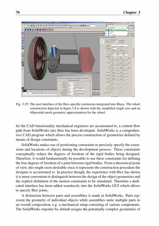
70 Chapter 3

Fig. 3.25: The user interface of the Ibex-specific extensions integrated into Maya. The wheelconstruction depicted in figure 3.8 is shown with the simplified single axis and anellipsoidal mesh geometry approximation for the wheel.

fer the CAD functionality mechanical engineers are accustomed to, a content flowpath from SolidWorks into Ibex has been developed. SolidWorks is a comprehen-sive CAD program which allows the precise construction of geometries defined bymeans of design constraints.

SolidWorks makes use of positioning constraints to precisely specify the exten-sions and locations of objects during the development process. These constraintsconceptually reduce the degrees of freedom of the rigid bodies being designed.Therefore, it would fundamentally be possible to use these constraints for definingthe free degrees of freedom of a joint between rigid bodies. From a theoretical pointof view, this might seem desirable since it represents the construction procedure thedesigner is accustomed to. In practice though, the experience with Ibex has shownit is more convenient to distinguish between the design of the object geometries andthe explicit definition of the motion constraints to be simulated. Therefore a dedi-cated interface has been added seamlessly into the SolidWorks GUI which allowsto specify Ibex joints.

A distinction between parts and assemblies is made in SolidWorks. Parts rep-resent the geometry of individual objects while assemblies unite multiple parts toan overall composition, e.g. a mechanical setup consisting of various components.The SolidWorks exporter by default assigns the potentially complex geometries of


a part to the Ibex visualisation geometry. Each part is assigned a set of physicsproperties which include the list of collision shapes. All information generated bythe Ibex extension is saved as user data in the original SolidWorks file. This ap-proach ensures a consistent coupling of rigid body dynamics information with thelogical CAD components while not affecting the further reusability of the designfor other purposes. Full access to the properties of the physical shapes is giventhrough a dedicated graphical user interface integrated into SolidWorks.

SolidWorks does not natively support the generation of wavefront *.obj geom-etry files as required by Ibex. Furthermore, SolidWorks is spline-based rather thanusing a vertex-polygon representation like the *.obj format. Therefore, a discreti-sation of the geometry needs to be performed by the Ibex extension when exportingan assembly. To this end, a simple *.obj file exporter has been developed and inte-grated into SolidWorks which uses native sampling and discretisation routines.

Both the Maya and the SolidWorks exporters generate as output an XML filefollowing a format specific to Ibex as well as the *.obj files for geometry definitionsand optionally image files for texturing objects in the visualisations. In section 3.1it was stated that existing file formats should be supported where possible. Thechoice was made to nevertheless develop a dedicated format for Ibex since no ex-isting definition fulfilled all the requirements at the time of development. For purerigid body dynamics setups, a number of formats exists which are typically linkedto an individual rigid body dynamics library. These formats lack features requiredin robotics simulations, such as sensor or actuator definitions. Further, it would beunwise for a simulation framework like Ibex to make a commitment to a specificrigid body dynamics library at the level of the data files as this might restrict the op-tions of further development. An effort is being made with the open-source ColladaXML standard to create an interchange format between applications for 3D assets[Col 06]. As part of version 1.4 (released in 2006, some time after the Ibex fileformat was specified), a physics simulation file format is included which definesbasic jointed rigid body models. This development should be closely followed andtaken into consideration in future extensions of Ibex.

Medieval Clockwork Example

Figure 3.26 a) shows the complex mechanics of a medieval clock exhibited at theLucerne Museum of History [HML 06]. The clockwork was originally containedin one of the towers of the town wall of Lucerne. The historically valuable artifactcannot be operated nowadays without risking damage to its structure. Therefore,the clockwork is being faithfully recreated as virtual model and simulated in Ibexin an effort to create an interactive museum exhibit which illustrates the operationof the clock to museum visitors. A model of the clockwork designed in Solid-Works and enhanced with rigid body dynamics properties using the Ibex extension

72 Chapter 3

a) b)

c) d)

Fig. 3.26: a) Medieval clockwork exhibited at the Lucerne Historical Museum. b) Physics-enhanced model of the clock designed in SolidWorks using the Ibex extensions.c) The same model simulated and visualised in Ibex. d) View of the physical ap-proximation exported from SolidWorks and visualised during an Ibex simulation.

is depicted in figure 3.26 b). A visualisation of the simulated clock in operationis shown in figure 3.26 c). The cogwheels of the real clock are of a rudimentarydesign, mostly containing cuboidal cogs instead of e.g. an involute profile. Thesesimple geometries can be approximated by cuboidal and capsule shapes in Ibex -precisely modelling the original design in the relevant contact regions. The simu-lated physical design is shown in figure 3.26 d) where the high number of individualcollision shapes can be appreciated.

The medieval clockwork relies on precisely calibrated collisions for correctoperation. The successful design and simulation of such an intricate mechanismdemonstrates the capabilities of the tool-chain established in Ibex. One aspectwhich has not been considered so far is the inclusion of active components whichapply forces and torques to the system. The dynamic behaviour of active compo-nents is most conveniently modelled in dedicated dynamic modelling software. Fol-


lowing the same argument employed when integrating Ibex-specific extensions into3D modelling tools, the following section describes how Ibex has been embeddedin a dynamic modelling and control engineering software, MathWorks Simulink

r.

3.3.6 Integration into Industry-Standard Dynamic Modelling Environment

So far, the simulation functionality of Ibex has been described and examples of thevisualisation capabilities shown in the illustrations. This functionality is includedin a software library which can be linked into stand-along application programs.

Stand-alone programs are typically specific to a single task for which predefinedphysical setups are loaded and simulated. This is partly due to the fact that activecomponents are controlled by algorithms within the compiled program code, thuslimiting their flexibility. The processing of sensor data is governed by the samelimitations. The user interface (which e.g. is an extension of the Ibex GUI) istypically also designed for a single application.

While such stand-alone programs are well-suited as final project outcome, theyclearly lack flexibility during the development process of an overall mechatronicsystem consisting of a passive mechanical setup, actuators, sensors and controllers.

A well-established software for modelling and simulating dynamic systems aswell as designing control algorithms is MathWorks Simulink

rwhich is based on

the MATLABr

numerical computing environment. Simulink has a visual program-ming interface in which blocks represent functions which operate on data flowsmodelled as connections between them. Numerous predefined blocks from a vari-ety of domains such as control engineering and signal processing exist which makeSimulink a versatile environment for rapidly designing and simulating dynamicsystems.

Simulink is designed with a block library architecture which can be extendedto include user-defined block libraries. User extensions can be written amongother languages in C/C++ and the native MATLAB M language. To integrate Ibexinto MATLAB/Simulink, a C++ block-set has been developed. This allows to co-simulate Ibex rigid body dynamics with all features available in Simulink simplyby using the Ibex blocks in the same way native Simulink blocks are used. As partof the integration, the Ibex graphics observer based on the Nebula 2 engine has alsobeen included into the Simulink user interface.

MathWorks markets a library named SimMechanics which also provides rigidbody dynamics simulations. In comparison with Ibex, its simulation kernel lackscollision detection and dynamic collision response based on physical properties. In-stead, merely kinematic constraints can be imposed on the system. SimMechanicsalso lacks any sensor simulation functionality beyond accessing the spatial vari-ables of bodies and joints. To obtain visualisations comparable to those offered byIbex, an additional MATLAB extension (the Virtual Reality Toolbox) must be in-

74 Chapter 3

stalled. For simulation content generation, an exporter for SolidWorks is providedby MathWorks. It parses a CAD assembly and generates an XML configurationfile which can be imported in SimMechanics. The information contained in the fileincludes mass and inertia properties of each part as well as joint definitions. Noinformation about the geometries or induced motion constraints is contained. Forvisualisations, the design must be exported separately using a VRML format.

The Ibex Simulink integration contains various categories of blocks. Systemblocks contain fundamental functionality and form the basis of any Ibex simulationin Simulink. One such block contains the core simulation functionality and theXML scene file loader. A second one encapsulates the Nebula 2 graphics observer:when the Nebula 2 block is placed on a Simulink model, the graphic engine opensa window when executing the model which contains the on-line visualisation of thescene. Since the graphics engine is executed in a separate thread, the visualisationis updated and can be inspected also when the simulation is paused.

A second category of Ibex blocks gives access to simulated entities. This in-cludes a block which represents a rigid object in the black-box abstraction describedin section 3.3.2. The output of the block consists of signals which represent posi-tion, orientation as well as the linear and angular velocities. To provide easy ac-cess to the fundamental rigid body characteristics of mass and inertia, these (time-invariant) quantities are also output as signals. The rigid body can be influenced byinput signals which represent forces and torques applied to the body.

The blocks giving access to joints function in a similar manner: for e.g. a rev-olute joint, its Cartesian position, angle (local joint position) and the orientationof the main joint axis are output. The inputs are designed in a way which allowseither to directly apply a torque to the joint or use a simple controller provided asstandard joint functionality by PhysX. This controller takes as inputs a desired rota-tional joint velocity and a maximal torque available. A further parameter specifieswhether the joint should be allowed to surpass the specified velocity unhinderedor whether a torque should be applied to prevent this from happening. Other jointtypes function similarly but do not contain any integrated controller functionality.

A next class of blocks allows to create rigid bodies from the Simulink userinterface. Such blocks exist for the basic shape primitives (sphere, cuboid, cap-sule) as well as for general mesh-shaped rigid objects. This functionality roughlycorresponds to the mechanism used in SimMechanics for creating rigid bodies, en-hanced by the specification of collision geometries. It has been found that withinthe overall work-flow rigid body creations from the Simulink GUI are well suitedfor simple objects e.g. used for debugging a construction by adding obstacles. Formore complex setups it has proven to be more convenient by far to use the 3Ddevelopment environments discussed in section 3.3.5.

An exception are specialised blocks used for the creation of terrains and envi-ronments in buildings. The terrain creation block operates as described in section


Fig. 3.27: The Simulink model used to control the map-drawing example illustrated in figure3.22.

3.3.3 and inserts a static mesh-based rigid body representing a terrain, optionallywith different material properties assigned to each triangle of the mesh shape. Thebuilding environment creation block is a convenient utility for creating a set of sur-faces, walls and ramps which approximate the structure of buildings. The blockparses a simple dedicated XML file and creates box-shaped rigid bodies with thespecified properties. The maze-like environment shown in figure 3.21 was createdusing this block.

Trigger shapes (cp. section 3.3.4) can also be created from the Simulink GUI.The single output port of these blocks indicates whether the geometry of the triggerintersects with any other shape in the simulation. Optionally, a list of rigid bodieswhich are excluded from producing an output can be passed to trigger blocks. Thiscan be important to avoid false reports of intersections. As example, the reportingof intersections between the sensor shapes and wheels of the robot shown in figure3.18 a) has been suppressed.

Contact notification blocks are used to monitor a pair of rigid bodies and re-port contacting conditions between those objects. An example application of theseblocks is the simulation of contact sensors. Another use from mobile robotics is thedetection of breaking ground contact of the wheels.

Further, there exists a block which outputs the measured distance of a range-finding sensor simulation following the physical model introduced in section 3.3.4.

The Simulink model used to drive the map-generation example illustrated infigure 3.22 is shown in figure 3.27. In the top row, the three blocks are the Ibexsystem block, the Nebula 2 graphics observer block and a building environment

76 Chapter 3

generation block respectively. Vertically aligned on the far right are three rota-tional joint blocks for accessing the three joint axes of the robot wheels. The blockdisplaying the same symbol near the left margin controls the axis which supportsthe sensor casing atop the robot. Above it, a rigid body access block provides thespatial coordinates of the robot chassis. In the bottom-left corner of the model,a distance sensor block outputs the readings of the simulated laser range-findingdevice.

All other blocks in the model contain standard Simulink functionality. In par-ticular, the path planning and trajectory tracking modules are programmed usingthe M language. Also the 2D plot of the sensor readings shown in figure 3.22 b) isdrawn by an M-file. An advantage of this approach (and a benefit of the Simulinkintegration) is the rapid development resulting from using the M language. This ispartly due to the simple yet powerful nature of this scripting language and partlygiven by the large amount of readily accessible MATLAB functionality. A draw-back is the relatively slow execution time of the interpreted M language in compar-ison with compiled programming languages such as C/C++. Especially the MAT-LAB graphics functionality has proven to be a significant bottleneck to system per-formance. In the map drawing example, the plotting of the two-dimensional mapconsumes more resources than the Nebula 2 graphics engine.

In general, the control logic of a robotic system (and other user-defined func-tionality) can be developed in Simulink using the M, C/C++, Java, Fortran and Adaprogramming languages. Alternatively, the functionality can be developed usingstandard Simulink blocks in the graphical programming environment.

A high level of flexibility is given when co-simulating Simulink models withIbex. Simulink can be freely configured to suit the requirements of the simulatedproblem. The options include fixed-step and variable-step integrations with a num-ber of different integration schemes. Ibex operates transparently with both fixedand variable time-steps in Simulink, itself always running with fixed time-steps.The Ibex module queries the Simulink simulation time when it gets called and ad-vances its simulation to the appropriate time-step in its own time-series. This timeis selected to be the Simulink time if possible or the last Ibex time-step before itotherwise. Clearly, this scheme performs best when the Simulink step size and theIbex step size are multiples of one another. In other cases correct simulation behav-iour is also obtained but the Ibex readings do not correspond to the Simulink timewhenever the time-steps do not coincide.

An important external interface is given by the Real-Time Workshopr

(RTW)extension of Simulink. The RTW allows to automatically generate target platform-specific program code from a Simulink model and compile it into a real-time appli-cation for that hardware. This capability permits to e.g. design and test a controllerbenefitting from the Simulink functionality and directly deploy the same controlleronto a real-time hardware target. Since user-defined blocks are excluded from the


RTW functionality, it is not possible to e.g. compile Ibex for a real-time target.From a rigid-body dynamics simulation point of view, the extension of

Simulink to include Ibex gives access to the complete MATLAB/Simulink func-tionality. In particular, being able to perform co-simulations with Simulink modelsallows to perform multi-domain dynamic system simulations. A typical applica-tion is the simulation of actuator characteristics in Simulink. The output of theSimulink actuator subsystem are forces and torques which are applied to the me-chanical structure being co-simulated in Ibex. Sensor readings can be output fromthe Ibex simulation as input to the control logic simulated in Simulink, thus closingthe feedback loop. This setup allows to simulate complete mechatronic systems,each component being located in an ideally suited simulation environment.

From a Simulink user’s point of view, the inclusion of Ibex simulations givesaccess to a powerful rigid body dynamics toolbox which includes a content gen-eration tool-chain integrated into well-established engineering solutions. As anadded benefit, collision detection, collision resolution, sensor simulations and theincluded visualisation capabilities can be named.

3.4 Validations and Performance

To illustrate the kind of precision which can be expected of Ibex simulations and theincluded AgeiaTM PhysXTM libraries in particular, a validation of simulation resultsis presented in the first part of this section. Thereafter, a performance analysis ofvarious simulation setups is presented. For all testing, version 2.2.0 of the PhysXlibraries has been used.

3.4.1 Validation of Simulations

The validations of simulation results are performed by studying relevant physi-cal phenomena in isolation. Simple physical setups are used to investigate uncon-strained rigid body dynamics, the effects of interpenetration between two collidingbodies, the characteristics of kinetic and static friction as well as rolling motion.

Unconstrained Motion

The behaviour of unconstrained rigid bodies has been validated by analysing theballistic trajectories of objects which are created moving at some initial velocity.For a rigid body released at a given initial linear velocity v0 with a positive elevationangle α, the peak height of the ballistic trajectory hpeak and the horizontal distancex(T ) travelled before returning to the initial height level are computed as followsassuming no aerodynamic drag:

78 Chapter 3

hpeak =v20 sin2(α)

2g(3.37)

x(T ) =v20 sin(2α)

g(3.38)

These analytical solutions have been compared to simulation results for integra-tion time-step values of ∆t = 0.1ms, 1ms and 10ms. The same time-step valueshave been used throughout the validation experiments since they cover the range offeasible settings for PhysX simulations. The simulation results obtained correspondwith the analytical solution to within numerical and discretisation precision. Thisnaturally leads to higher precision being achieved at smaller time-steps. Conser-vation of energy can be observed for unconstrained motion considering both linearand angular velocities:

Etotal = Epot + Ekin lin + Ekin rot = mgh+mv2

2+Iω2

2= const (3.39)

where I represents the inertia tensor corresponding to the rotation axis and ω the an-gular velocity of the body about that axis. The simulation results for unconstrainedmotion of rigid bodies match the expected behaviour at a fidelity which renderssuperfluous further analyses. The following sections deal with the more interestingcases where dynamic constraints apply to the motion of the rigid bodies.

Rigid Body Collision and Rebound

To study the behaviour of colliding rigid bodies, a setup is employed where oneobject is dropped onto a second one which is statically anchored in the scene. Thebasic setup consists of a sphere shape with radius r = 1m dropped onto a planefrom a height of h = 10m. The experiment has been repeated for 20 differenttime-step settings ranging from ∆t = 0.1ms to ∆t = 50ms. The largest time-steps are outwith the practicable range but are nevertheless included to illustratethe degradation of precision.

The collision resolution behaviour is determined by the coefficient of restitu-tion which specifies the proportion of kinetic energy remaining in the objects afterthe collision. Analytically, an energy conservation formulation is used, again dis-regarding air drag. The initial energy of the object can be computed as

E = Ekin(tfirst impact) = Epot(t = 0) = m · g · h(t = 0) (3.40)

Similarly, the energy after the first impact can be formulated as:


Fig. 3.28: Plot of the object’s height above ground as function of time during collision res-olution in the rigid body collision experiment. The general characteristics can beobserved during all collision experiment runs. Importantly the interpenetrationlasts no longer than one time step.

E′ = cr · E = Epot(t1) = m · g · h(t1) (3.41)

with cr the coefficient of restitution and t1 the time at which the object reaches themaximal height after the first rebound. In the setup described above, the coefficientof restitution directly specifies the height of the first rebound:

h(t1) =cr ·m · g · h(0)

m · g= cr · h(0) (3.42)

Hence, in the experiment the height of the first rebound is measured for differenttime-step sizes. The second measure used to determine the quality of collisionresolution is the maximal amount of penetration on collision. Figure 3.28 shows atypical plot of the height of the object above ground as function of time which isfound in this form for all performed collision experiments. The two bodies can beobserved to intersect for no longer than one time step.

The plot shows that the penetration depth depends not only on the selectedtime-step size but also on the height above ground at the last time-step before theinterpenetration. This height can be beneficial or detrimental to the penetrationdepth, depending on the relative approximation velocity of the two bodies. Figure3.29 a) shows how the error on rebounding as well as the penetration depth dete-riorate with increasing time-step size. The depicted plot has been generated fromthe experiment involving a sphere dropping on a plane. The equivalent experimentshave also been conducted for all combinations of a mesh collision shape approxi-mation of the sphere and a cuboidal primitive (all edge lengths li = 2m) droppingon both a plane and a cuboid. The results for all experiments are virtually identical,the largest deviation in terms of rebound height being 0.1mm and for the penetra-tion 4.5mm. Varying the restitution coefficients also results in equivalent outcomesof the experiment.

An interesting observation is that the rebound height is consistently too highin all measurements, on average by 1%. A possible hypothesis to explain this

80 Chapter 3

a) b)

Fig. 3.29: a) Validation results for saltation test using a sphere of radius 1m dropping ontoa ground plane from 10m height. The plot shows the relative rebound heighterror after the first impact (circles, left ordinate axis) and the penetration depthson impact with the ground plane (x-markers, right ordinate axis) as function ofthe selected simulation time-step. b) Study of relative rebound error as functionof penetration depth for a time-step of ∆t = 10ms.

energy gain is that the penalty forces applied during collision resolution are notcompletely compensated by the solver. To follow-up this issue, the relative rebounderror is plotted against the penetration depth in figure 3.29 b) for a static time-step size of 10ms. The initial height is varied minimally to control the amount ofpenetration. The shown plot is obtained from the sphere-on-plane experiment butis representative for all object pairs studied. The results are contrary to what mightbe expected, as smaller penetration depths lead to larger rebound errors. The figurealso gives an idea of the variations which could be expected for the results shown infigure 3.29 a) by changing the initial height such that the penetration depth rangesbetween 0 and the amount travelled by the bodies towards one another in a singletime-step.

Kinetic Friction

The next physical phenomenon analysed is kinetic friction which is investigated byusing an inclined ramp down which various objects are made to glide. Given theelevation angle α of the slope, following forces can be analytically computed: thenormal Fg⊥ and tangential Fg‖ components of the gravitational force Fg = m · gas well as the (kinetic) friction force Fk opposed to the tangential force:

Fg⊥ = cos(α) · Fg = cos(α) ·m · g (3.43)Fg‖ = sin(α) · Fg = sin(α) ·m · g (3.44)


Fk = µk · Fg⊥ = µk · cos(α) ·m · g (3.45)

Assuming the body slides down the slope due to Fg‖ being larger than Fk andany applying static friction, the resulting force Fres is parallel to Fg‖ with

Fres = Fg‖ − Fk = m · g · sin(α)−m · g · cos(α) · µk (3.46)

The acceleration of the body down the slope can thus be computed as

x =Fresm

= g · (sin(α)− µk · cos(α)) (3.47)

Under the assumption that no initial positional offset or velocity are applied,the equation for the position along the slope

x(t) =x · t2

2=g · (sin(α)− µk · cos(α)) · t2

2(3.48)

can be solved for the kinetic friction coefficient µk:

µk =−2 · x(t)

t2 · g · cos(α)+ tan(α) (3.49)

The validation experiment for dynamic friction consists of analysing 21 objectswith kinetic friction coefficients µk = i ·0.05 | i = 0..20 and static friction µs =0. The time required by the objects to traverse a trajectory of given length downthe slope is measured and the observed kinetic friction coefficient µ′k determinedusing equation 3.49. Three different integration time-steps have been tested: ∆t ∈0.1ms, 1ms, 10ms for 17 different inclinations α = j · 5 | j = 1..17. Theresults for cuboidal primitives sliding down the ramp (which is also modelled ascuboid) are shown in figures 3.30 a), c) and e) for the three time-step sizes. Theanalogous experiments for polygonal mesh shapes of identical cuboidal geometryleads to results which correspond to within a fraction of a percentage point.

A flat cylinder modelled as mesh shape produced the somewhat different re-sults depicted in figures 3.30 b), d) and f). They remain equal in nature to thecuboid results but display some quantitative differences. The worst correspondenceis found for ∆t = 0.1ms. There, the means of the observed kinetic friction coef-ficients µ′k corresponding to each input (PhysX) kinetic friction coefficient µk dif-fer by a maximum of |µk − µ′k| < 0.09 or 12%. The values µk ∈ 0.0, 0.05result in significantly higher relative discrepancies despite absolute deviations|µk − µ′k| < 0.003. For time-step sizes ∆t = 1ms and ∆t = 10ms the devi-ations are |µk−µ′k| < 0.015 or 3.5% and and |µk−µ′k| < 0.03 or 6% respectively.

The above mentioned comparison excludes the results for ∆t = 0.1ms andα = 80 since this setup appears to represent some sort of singularity. Plots 3.49 a)and b) show the significant deviation of those measurements which only occur in

82 Chapter 3

a) b)

c) d)

e) f)

Fig. 3.30: Plots of kinetic friction validation: observed kinetic friction coefficient plotted asfunction of kinetic friction coefficient input into PhysX libraries. a) cuboid, time-step ∆t = 0.1ms b) cylinder, ∆t = 0.1ms c) cuboid, ∆t = 1ms, d) cylinder,∆t = 1ms, e) cuboid, ∆t = 10ms, f) cylinder, ∆t = 10ms.


Fig. 3.31: Second-order polynomial fitting of mean measured kinetic friction values withstandard deviation (1ms experiments). Inverse function which can be used totransform a desired kinetic friction value into an input to the PhysX libraries.

a neighbourhood 79.999 < α < 80.001. To obtain a non-singular value whichfalls in line with the other measurements, in the analysis the value µk(80) hasbeen replaced by µk(80) = µk(79.999)+µk(80.001)

2 .All objects have been assigned a static friction coefficient µs = 0. This leads to

situations where µk > µs which are not considered when using traditional conven-tions. The result of such settings is in the PhysX libraries that some objects withµs = 0 nevertheless do not commence to slide down the ramp. This is presumablycaused in discrete time by a potential first non-zero velocity being prevented bythe kinetic friction which is already included in that time-step. Results for morecombinations of µs and µk are presented in the following section which deals withstatic friction.

From the results shown in figure 3.30 it is obvious that the PhysX librariesuse a different convention for dynamic friction from the one used so far in thisdocument. If the definitions were identical, the plots would show a (linear) equalitycorrespondence µ′k = µk. Further, values of µ′k > 1 have been registered, whichlead to Fk > Fg⊥ for µk ' 0.7.

This scaling as well as the non-linearity can either be accepted as part of thesimulated physics model or compensated by selecting appropriate values for theinput PhysX µk. Figure 3.31 shows how the computed kinetic friction values canbe approximated by a second-order polynomial using polynomial regression. Theexample shown is based on all data (cuboid, mesh cuboid and mesh cylinder) at∆t = 1ms. The approximation lies well within the standard deviations of theoriginal data. Consequently the inverse function of the polynomial (also shown inthe figure) can be computed and used to pre-process a desired kinetic friction value

84 Chapter 3

in order to obtain the input to PhysX which leads to the expected results.This technique could be extended to all time-steps and generalised in order to

include it in a framework such as Ibex. While such a feature is easy to integrate,it has been preferred not to do so and pass on the default PhysX behaviour to theusers. Given the degree of deviation in dependence of time-step size and involvedobject geometries, it is advisable to closely study the characteristics of a specificinteraction in situations where a high degree of accuracy is desired.

Static Friction

The static friction model has been tested in a setup consisting of 21 objects withstatic friction coefficients µs = i ·0.05 | i = 0..20 placed on a horizontal surface.A horizontal force of a magnitude increasing linearly over time has been applied tothe centre of mass of the objects. The moment when the objects start to move andthe corresponding break-free force Fb have been recorded. This allows to determinethe observed static friction coefficient for this setup (α = 0):

µ′s =FbFg⊥

=Fb

cos(α) ·m · g=

Fbm · g

(3.50)

The results of the static friction experiments are shown in figure 3.32, againfor the time-step sizes ∆t ∈ 0.1ms, 1ms, 10ms and both the cuboidal primitiveand flat polygonal mesh cylinder already used for previous validations. As in thedynamic friction validation, a mesh shape of identical geometry as the tested cuboidyielded practically indistinguishable results.

The effect described above where kinetic friction plays the role of static frictioncan be observed for all cases where µk > µs. Also, the same scaling observed inthe dynamic friction validation (with µk = 1 µ′s ≈ 2.03) is evident. Taking intoaccount these effects, the results for the mesh cylinder and ∆t = 10ms shown infigure 3.32 f) approximate the desired behaviour. For µk = 0, the force requiredto set the object into motion depends linearly on the static friction coefficient. Forµk < µs the same force is required. If (against the usual convention) µk > µs, thekinetic friction coefficient prevents any starting of motion.

The other experiments reveal differing behaviour of the studied objects: Thelinear behaviour for µk < µs can be observed in many cases, but mostly µ′s is notindependent of µk. This effect can be seen well in figure 3.32 e) (cuboid, ∆t =10ms) where for µk = 0 a linear dependence of µ′s = c · µs is evident but with acoefficient c ≈ 1.3 instead of c ≈ 2. For increasing values of µk, the correspondingcoefficient increases (albeit not monotonically) such that for µk ∈ 0.8, 0.9, avalue of nearly 2 is reached and for µk = 1 a constant µ′s ≈ 2.03 is again attained.

The experiments for ∆t = 1ms correspond well to their 10ms counterparts forµk < 0.5 and µ′s / 1 as well as for µk > 0.8. The intermediate interval results


a) b)

c) d)

e) f)

Fig. 3.32: Plots of static friction validation: observed static friction coefficient plotted asfunction of static friction coefficient input into PhysX libraries. a) cuboid, time-step ∆t = 0.1ms b) cylinder, ∆t = 0.1ms c) cuboid, ∆t = 1ms, d) cylinder,∆t = 1ms, e) cuboid, ∆t = 10ms, f) cylinder, ∆t = 10ms.

86 Chapter 3

in differing values of µ′s for the cases where kinetic friction prevents the motion.Furthermore, objects start to move at forces lower than those expected with thepreviously discussed behaviour. Also, a quantisation of required break-free forces(and hence µ′s) can be observed for 0.5 ≤ µk ≤ 0.8 with µ′s ' 1: objects ofdifferent friction coefficients commence to move at precisely the same time-step.In one case (for the mesh cylinder with µk = 0.2), an object of higher µs breaksfree at a lower “quantum” than its next lower neighbour.

At a time-step of ∆t = 0.1ms, the divergence of the linear coefficient describedabove is even more pronounced, ranging from c ≈ 0.65 (cuboid, figure 3.32 a)) toa similar final value of c ≈ 2.03 for µk = 1. A distinct non-linearity is present inthe range 0.15 / µs / 0.5 where to some extent a similar effect to the quantisationdescribed in the ∆t = 1ms experiments can be perceived.

Contrary to the dynamic friction model, which in itself appears consistent, thecombined static friction model (including both µs and µk) has produced resultswhich are difficult to map onto the conventional friction definitions. For experi-ments which rely on precise break-free forces it is imperative to study the concreteinteraction in detail to obtain a meaningful prediction.

Rolling Motion

The last basic interaction included in this validation deals with rolling motion. Thesetup used is similar to the one presented for the kinetic friction experiments: aramp is inclined at various elevation angles α and the progress of various initiallyresting objects studied as they move down the slope. As test objects, a sphere, acapsule primitive and a cylinder approximated as polygonal mesh (with the periph-ery composed of 72 planar surfaces) are used. Analytically, the tangential forceFg‖ acting on a body rolling down a slope can be decomposed into a linear and anangular component:

Fg‖ = Ftrans + Frot = m · a+τ

r(3.51)

where τ is the torque which is τ = I · ω with I the inertia tensor and ω the angularvelocity. The angular acceleration ω of a body rolling down a slope rotating aboutan axis at a constant distance r from the slope can be computed as ω = a

r . Equation3.51 can hence be transformed into

Fg‖ =(m+

I

r2

)· a (3.52)

Inserting equation 3.44 (which is purely geometric and hence also holds truefor the rolling case) into equation 3.52 and solving for the (linear) acceleration ayields:


a =sin(α) ·m · gm+ I

r2

(3.53)

For the bodies involved in the experiment, the inertia tensors (for rotations aboutthe symmetry axis) are as follows:

Isphere =25msphere · r2 (3.54)

Icylinder =12mcylinder · r2 (3.55)

Icapsule = Icylinder + Isphere =(

12mcylinder +

25msphere

)r2

= ρcapsuleπr4

(h

2+

815r

)(3.56)

with ρcapsule denoting the density of the capsule, which is assumed to be homoge-nous. For the last equality in equation 3.56, the formulas for the volume of a cylin-der and sphere have been used. Applying x = x·t2

2 , the formula for the distancetravelled by a mass under constant acceleration and solving for the time gives fol-lowing expressions for the three bodies:

Tsphere =

√14 · x(T )

5 · g · sin(α)(3.57)

Tcylinder =

√3 · x(T )g · sin(α)

(3.58)

Tcapsule =

√x(T )

(3h+ 56

15r)

g · sin(α)(h+ 4

3r) (3.59)

The validation results for the sphere are shown in figure 3.33, those for themesh cylinder in figure 3.34 and the results for the capsule in figure 3.35. Theanalytical solution for rolling motion presented above applies to perfect rollingmotion, i.e. when no sliding occurs. In the experiments a combination of slidingand rolling motion can often be observed. Analytically, exclusively sliding motionoccurs at µk = 0. As soon as some friction is present, a torque is induced inthe sliding bodies which consequently commence to roll in combination with thesliding motion. At the point where the friction force Fk becomes larger than thetangential component Fg‖ of the gravitation force, i.e. µk · cos(α) > sin(α), the

88 Chapter 3

a) b)

c) d)

Fig. 3.33: Plots of rolling validation for sphere shape: times T required by object to traversea trajectory of fixed length x(T ) = 3m. a) Analytical solution with kinetic fric-tion coefficient µk clamped to zero for non-rolling motion. b) simulation results,time-step ∆t = 0.1ms c) ∆t = 1ms d) ∆t = 10ms. Note the differing ordinatescaling of the analytical plot.

body displays an exclusively rolling motion. Figures 3.33 a), 3.34 a) and 3.35 a)show the results of a combined analytical solution for sliding and rolling motion.To improve the readability of the graphs, it has been assumed that the objects areeither perfectly sliding (µk = 0) or perfectly rolling.

The value of µk at which an object displays overwhelmingly rolling motiondiffers strongly for the three object types. This “rolling boundary” is the lowestfor the capsule shape, followed by the mesh cylinder (ca. ∆µk = +0.05 behind)and the sphere. The rolling boundary of the sphere increases from a similar level atsmall ramp inclinations to requiring µk = 1 to roll at α = 45. At that inclination,


a) b)

c) d)

Fig. 3.34: Plots of rolling validation for cylindrical mesh shape: times T required by objectto traverse a trajectory of fixed length x(T ) = 3m. a) Analytical solution with ki-netic friction coefficient µk clamped to zero for non-rolling motion. b) simulationresults, time-step ∆t = 0.1ms c) ∆t = 1ms d) ∆t = 10ms. Note the differingordinate scaling of the analytical plot.

the other shapes already commence to roll with µk ≈ 0.6, and continue rollingup to α ≈ 60. A graphical representation of the rolling boundary is shown infigure 3.36.

Considering the situations where objects do largely display rolling mo-tion, little difference in the time required to traverse the given distance canbe distinguished. For ∆t ∈ 0.1ms, 1ms, the times differ by less than|Ti − Tj |i,j∈sphere, cylinder, capsule < 0.5%. In particular, this means that theinertia tensor appears to play a negligible role in the computations. The absolutetimes measured for the objects to traverse the distance are approximately a factor 5

90 Chapter 3

a) b)

c) d)

Fig. 3.35: Plots of rolling validation for capsule shape: times T required by object to tra-verse a trajectory of fixed length x(T ) = 3m. a) Analytical solution with kineticfriction coefficient µk clamped to zero for non-rolling motion. b) simulation re-sults, time-step ∆t = 0.1ms c) ∆t = 1ms d) ∆t = 10ms. Note the differingordinate scaling of the analytical plot.

higher than expected, despite all artificial angular damping having been suppressedin the PhysX libraries.

At a simulation time-step of ∆t = 10ms, larger discrepancies can be observedin the traversal times of the three bodies at different ramp inclinations. In partic-ular, the mesh cylinder displays a wide spread of times. This can be explained byits periphery being composed of 72 planar surfaces which cause some amount ofsliding motion, even above the nevertheless discernible rolling boundary.


a) b) c)

Fig. 3.36: Graphical representation of the rolling boundary for the three studied bodies. Thelowest values of µk (red) correspond to setups where only the capsule shape dis-plays rolling motion to an overwhelming extent while the other shapes mostlyslide. The next band (yellow) indicates situation where both the capsule and themesh cylinder roll, but not the sphere. The highest values of µk (green) indicaterolling motion for all three objects. a) time-step ∆t = 0.1ms, b) ∆t = 1ms,c) ∆t = 10ms.

3.4.2 Performance Analysis

The most versatile configuration of Ibex is when it is used embedded in Simulink.Other than for dedicated single-application tasks it is presumably the setup mostlikely to be used for most simulations. Therefore, the performance tests presentedin this section are based on the Ibex-Simulink integration, despite this configurationimplying an overhead in terms of processing power and memory usage.

The test computer has an Intelr

CentrinoTM 1.6GHz CPU, 1GB RAM and anATI MobilityTM Radeon

r9000 GPU with 64MB VRAM. The operating system is

rWindows

rXP Professional with Service Pack 2 (SP2) installed. No particular

effort has been made to improve the performance of the system (e.g. by deactivatingsystem tasks etc.).

The basic test setup for the performance measurements consists of a stack of50 objects placed on a plane. The topmost object is positioned with a minimalhorizontal offset relative to all others. When the simulation commences, this offsetcauses the entire stack to topple over under the effects of gravity. Such a setup leadsto numerous collisions between the objects, from the average two for each objectinitially (with its upper and lower neighbour) to a varying number with varyingcollision partners as the stack collapses. For each experiment, the time required toprogress the simulation 30s (roughly the time required by the objects to all be in

92 Chapter 3

a) b)

Fig. 3.37: Plots of real-time coefficients and simulation times for a collapsing stack of 50objects simulated for 30s. a) with Nebula 2 observer window at a resolution of1024×768 pixels, b) without graphics output.

contact with the ground) is determined. The real-time coefficient is defined as

cRT =trealtsim

(3.60)

with treal the duration of the process (30s) and tsim the time required to simulate it.For a simulation to run in real-time, it must fulfill cRT = 1. If it progresses faster, itcan be artificially slowed down to achieve real-time behaviour. In the opposite casethe setup cannot be simulated in real-time with the given resources. Real-time be-haviour is of particular importance where other entities which run in real-time relyon interactions with the simulation. Hardware-in-the-Loop (HIL) simulations con-sist of real-time simulations which interact with hardware devices (such as controlelectronics or actuators etc.) [Hanselmann 93], [van Amerongen 03]. HIL tech-niques are useful to e.g. test and study the behaviour of hardware devices in acontrolled environment.

The different operation modes of the simulation environment have been intro-duced in section 3.3.1. While not directly applying to the Simulink integration,Ibex is run at “CPU-speed”, i.e. as fast as possible for the performance tests. Inall experiments, the time-steps of Ibex and Simulink have been synchronised (cp.section 3.3.6).

Figure 3.37 shows the results of simulating a collapsing stack of 50 objects.As object geometries, sphere primitives, cuboidal primitives and polygonal meshrepresentations approximating the sphere shape have been used. The mesh sphere


consists of 212 vertices and 420 triangles. To mitigate the impact of external in-fluences on the performance measurements, each experiment has been repeated 5times. Figure 3.37 shows the mean values and standard deviations of these mea-surements. In the experiments shown in figure 3.37 a), a Nebula 2 graphics observerwindow has been used to visualise the simulation at a resolution of 1024×768 pix-els. The results closely correspond for the sphere primitives and the polygonal meshapproximations thereof. This is somewhat surprising as a sphere is a significantlysimpler geometry to simulate - a sphere-sphere collision detection can be reducedto determining the distance between the two sphere centres and comparing it to thesum of both radii. The cuboid primitives are simulated at the highest real-time co-efficient. All objects display an approximately linear dependency on the time-stepsize which corresponds to the expected outcome.

Figure 3.37 b) shows the results of the same experiments without any graphicaloutput. Abandoning the visualisation results in a significant performance boost.The setup can be simulated faster than real-time even for the smallest tested time-step of 1ms. Without graphics observer, spheres are clearly simulated at the highestvelocity. The time required to simulate the setup for cuboids and the mesh sphereapproximations is similar. The analysis of exclusively the simulation performancereveals the reason for the unexpected performance equality of sphere primitivesand polygonal mesh approximations discussed above. In the graphics engine, boththe spheres and the mesh approximations are visualised using the same geometry.The performance of the graphics engine appears to be the determining factor of theoverall performance. This causes the cuboid experiment (which involves a simplervisualisation geometry) to run faster than the two experiments involving spheres.

This hypothesis is supported by the graphics frame rates observed in the exper-iments visualised in figure 3.37. The amount of resources available to the graphicsengine is determined by a load-balancing algorithm. In the tested configuration,the total of available resources is distributed at a constant ratio between a workerthread running the simulation and the visualisation thread. Hence (assuming thetotal resources remain constant during the duration of the experiment), the com-plexity of the visualised scene determines the graphics frame rate. Both sphereexperiments run at an approximate 73FPS, while the cuboid experiment displaysaround 110FPS. This proportion of ca. 2:3 corresponds roughly to the performanceratio of the associated experiments. Clearly, the load-balancing scheme tested isnot optimised for maximal simulation velocity - but arguably the use of a complex3D graphical visualisation conflicts with such a target in the first place. An alter-native load-balancing algorithms would behave like the described scheme at highsimulation loads but limit the resources available to the graphics engine in a waythat its performance does not exceed a specified upper limit, e.g. 30FPS. If moreresources were available to the visualisation thread, it could renounce them, thusbenefiting the simulation thread.

94 Chapter 3

Fig. 3.38: Overall simulation performance as function of Nebula 2 graphics observer resolu-tion. Real-time coefficient cRT represented as mean and standard deviation of 5experiments as well as corresponding mean execution times shown. Experimentsetup: one stack of 50 spheres.

The influence of the visualisation resolution on the simulation performance isshown in figure 3.38. Different standard resolutions have been applied to the graph-ics observer window and the overall performance of the simulation measured. Asexperiment, a stack of 50 sphere primitives is used with the same visualisation set-tings as before. The frame rates of the graphics engine vary between 57FPS for thehighest 1600 × 1200 pixel resolution and 93FPS for the lowest 320 × 240 pixelresolution. As above, the mean values and standard deviations of five simulationruns are shown together with the corresponding mean execution times. Again, itcan be observed that the frame rates correspond well with the real-time coefficientdue to the load-balancing algorithm employed.

The performance of Ibex simulations as function of scene complexity is vi-sualised in figure 3.39. Departing from the original setup of 50 stacked spheres,experiments have been run which include repeated identical stacks. The stacks arepositioned in a way which prevents any interaction between spheres from differentstacks. This ensures that a setup containing n stacks not only consists of n · 50spheres but also only leads to n times the original number of collisions. Figure3.39 a) shows the results of simulation runs which are visualised using a Nebula 2observer at a resolution of 1024×768 pixels. Mean values and standard deviationsfor cRT of five experimental runs for each setup are shown, as well as the corre-sponding simulation times tsim. The analogous plots for the experiments withoutgraphical output are shown in figure 3.39 b). The simulation times required byboth experiments are roughly linear with the scene complexities within the testedrange. The rate of increase somewhat reduces for higher complexities in the setup


a) b)

Fig. 3.39: Plots of real-time coefficients for different numbers of collapsing stacks contain-ing 50 spheres each. Values on the abscissa indicate total number of spheres inthe scene. Simulation time is tsim = 30s. a) with Nebula 2 observer window at aresolution of 1024×768 pixels, b) without graphics output.

including the graphics observer. A possible explanation therefore is that in the morecomplex scenes increasingly more objects are eliminated in the graphics engine byculling algorithms since they are either outwith the field of view or obscured byother objects.

The plot shown in figure 3.39 b), covers the experiments without visualisation.For scenes including more than ca. 500 spheres, a linear growth of measured ex-ecution times tsim can be recognised. This trend is confirmed by experiments for2000, 3000, 4000 and 5000 spheres not shown in the plot. For small scenes (belowca. 300 spheres) an approximately linear behaviour can also be measured, with alower rate of increase. The transition between the two models can hypotheticallybe explained by the increased memory consumption, e.g. some data structure notfitting in cache memory or inducing higher management overhead from a certainscene size on.

An alternative measure for scene complexity involves not increasing the numberof objects in the scene but rather the complexity of each simulated object. To thisend, a setup has been simulated which includes a stack of 50 polygonal mesh cubes.In the simplest setup, the cubes are represented by their 8 corner vertices and thecorresponding 12 triangles (6 triangulated quadratic faces). More complex meshcubes are created by subdividing each face into a number of smaller triangulatedquadratic surfaces. Applying the same number of subdivisions s along each axisof the cube results in v = 6s2 + 2 vertices and f = 2 · 6s2 triangular faces. Fors→∞, the proportion becomes f

v → 2. The results for the experiments involvingdifferent object complexities are shown in figure 3.40. In figure 3.40 a), the setupincludes a Nebula 2 graphics observer running at a resolution of 1024×768 pixels.A linear dependency on the total object complexity - represented on the abscissa by

96 Chapter 3

a) b)

Fig. 3.40: Plots of real-time coefficients for a single collapsing stack containing 50 polygo-nal mesh cubes. Values on the abscissa indicate the number of polygon faces oneach of the 50 objects. Simulation time is tsim = 30s. a) with Nebula 2 observerwindow at a resolution of 1024×768 pixels, b) without graphics output.

the number of polygons contained in each object - can be discerned. Comparing thisresult with figure 3.40 b) where the results for the equivalent experiments withoutvisualisation are shown indicates to the dominating influence of the graphics enginewhich leads to this linear behaviour.

Without any visualisation, a somewhat surprising outcome is the non-monotonic increase of computation times with increasing object complexity. Asignificant minimum can be recognised around the measurement containing objectswith 56 surface subdivisions (37’632 faces). The exact cause of this phenomenoncould not be established without gaining access to the PhysX algorithms. Specula-tive explanations include that vertices on the objects are culled to a certain degreebeginning at some object complexity. A further hypothetical explanation is thatsome aspects of memory management are altered with complex objects. Measure-ments for 128 subdivisions of each cube face cause the Nebula2 graphics engine tocrash, they are consequently omitted in the plots. Without visualisation, a real-timecoefficient of cRT ≈ 0.2 is achieved, corresponding to 143s execution time on thetest computer. On the one hand this demonstrates the capabilities of the PhysXlibraries to perform fast computations of complex setups. On the other hand, thisvalue closely corresponds to the linear extrapolation of the measurements for rela-tively low complexities, somewhat putting into perspective the significance of theminima at 56 subdivisions.

To round off the performance analysis, an example is presented which givesan impression of the performance achieved with a more realistic system includingjoints and active components. The medieval clockwork already introduced in sec-tion 3.3.5 has been embedded in a structure including a hand (At that time a singlehand was used to indicate the time), the dial as well as two bells. The clockwork


Fig. 3.41: The complete setup of the medieval clockwork visualised in an Ibex simulation.

is operated as in reality: the source of power is given by a weight attached to arope wound around a drum. The pendulum regulates the velocity of the gears usingan escapement mechanism. In the simulation the force exerted by the weight is ap-plied directly to the drum as constant torque. This is the only source of power in thesetup. The torque is sufficient to keep the pendulum swinging and the clockworkmoving exclusively through the rigid body collisions between the gears and leversinvolved.

The complete setup is depicted in figure 3.41. The scene consists of 28 rigidobjects, composed of 730 individual collision primitives, cp. figure 3.26 d) for avisualisation of the collision shapes. A total of 26 rotational joints hold the cog-wheels in place and define the motion of the clockwork. On the same test computerused throughout this section, the setup can be simulated in Simulink at ca. 27×real-time using a time-step of 0.01s. When adding a Nebula 2 observer for visual-isation (at a resolution of 1024×768 pixels), the performance drops to cRT ≈ 0.2due to the complexity of the involved artwork. When running as a stand-alone ap-plication instead of embedded in Simulink, the same setup yields a performanceof cRT ≈ 1.06, hence faster than real-time. This would allow to build a museumexhibit of the clockwork operating in real-time together with the visualisation onhardware of similar performance as the test computer.

98 Chapter 3

Hardware-Accelerated Physics Simulation

One important aspect to take into consideration when discussing the performancecharacteristics of Ibex and in particular the AgeiaTM PhysXTM libraries is theavailability of hardware-accelerated simulation libraries. In Spring 2006, Ageialaunched its physics processing unit (PPU) also named PhysX.

The PhysX PPU is shipped embedded in an add-on PCI express card for per-sonal computers and consists of a dedicated parallel hardware architecture op-timised for computing the type of operations required by physics simulations.Physics simulations in this context include not only rigid body dynamics but alsoparticle systems, deformable objects (e.g. cloth simulations), liquids and fracturesof bodies among other things.

One manufacturer of PCI cards containing the PhysX chip, BFG Technolo-gies ([BFG 06]) states 530 million sphere-sphere collisions per second and 533’000convex-convex collisions per second as maximal real-time capabilities of their card.Such performance characteristics would open completely new possibilities of sim-ulation for robot motion planning. For example it would become tractable to simu-late a large number of individual pebbles as terrain model. This would offer a newlevel of detail when simulating the interaction of robot wheels with the terrain.

The latest PhysX libraries required to perform hardware-accelerated physicssimulations have not yet been integrated into Ibex. However, the possibilities of-fered by hardware-supported physics make this a promising extension for the futuredevelopment of the simulation framework.

3.4.3 Limitations of Simulation Approach

The possibilities of rigid body dynamics simulations have been demonstrated inthis chapter by means of an introduction to the theoretical background as well asapplication examples of the Ibex framework. In this section some limitations ofthe simulation approach are discussed to complete the picture given of rigid bodydynamics simulations in general and the Ibex framework in particular.

One of the major bottlenecks when attempting to create a genuine model ofreality in a simulation is the availability of adequate data. Often, mechanical se-tups are simulated whose characteristics are not exactly available. To perform asimulation, precise values must be provided to the algorithms thus requiring someassumptions to be made about the physical system. In the case of a mechatronicsystem, the properties of the setup are usually known with a good precision. For anon-trivial terrain model on the other hand, data availability often is sketchy and af-flicted with errors. Interpolation errors such as the arbitrary choice of triangulationdirection discussed in section 3.3.3 introduce further discrepancies when modellingsome specific terrain. A decrease of simulation accuracy due to limited data avail-ability is not intrinsic to rigid body dynamics but rather a general problem of any


simulation approach.In the presented rigid body dynamics techniques, discretisation errors also oc-

cur when approximating parametric curves of objects through piecewise linearpolygonal geometries. The counterargument can be upheld that any arbitrary pre-cision can be achieved with a polygonal approximation, albeit at the cost of in-creased computation times. This tradeoff between precise geometry approximationand computational costs is exploited when using primitive shapes to approximatecomplex geometries. Indeed it can be seen as an important strength of the pro-posed approach to specify the relative importance of computational velocity andsimulation precision.

A fundamental parameter which is inherent to all discrete-time simulations isthe simulation time-step. The time step usually directly corresponds to the inte-gration step introduced in section 3.3.2. Smaller time-steps allow more accuratecomputations of the simulated system. Larger steps allow faster progress in timewhile accepting a potential reduction in accuracy. Additional deviations from theexpected behaviour arise with large time-steps when the contact detection schemeallows interpenetrations of rigid bodies, i.e. no continuous collision detection isused (cp. section 3.3.2).

Discrepancies from the behaviour of a real-world system also arise from therigidity assumption which strictly speaking does not hold true for virtually any ob-ject. Notwithstanding, many objects of interest in mechatronic systems can be ap-proximated as rigid objects in a way which yields acceptable simulation results. Asa side note, paradoxically, the two inaccuracies introduced by allowing interpene-tration as consequence of discrete simulation time-steps and the rigidity assumptioncause opposing errors and can cancel each other out. Jointly (and together with anappropriate restitution model) these effects can result in a level of approximationwhich corresponds to an elastic deformation at collision time.

Finally, the potentially chaotic behaviour of multi-body systems needs to bementioned. In unstable configurations, small differences of local characteristics(either static properties or dynamic physical behaviour) lead to considerably dif-ferent global behaviour. As an example, consider a spherical body balanced ontop of a prismatic object forming an infinitesimally sharp ridge, cp. figure 3.42.Clearly this is an unstable equilibrium and the slightest perpendicular force appliedto the sphere will set it in downwards motion over the side of the prism due tothe gravitational pull. As a consequence of this motion, the potential energy ofthe sphere is transformed into kinetic energy. The moving sphere can then applyforces of a magnitude significantly larger than those required to originally set itin motion to other objects (not shown) in the setup. Furthermore, the direction ofthe originally applied force determines in which direction the sphere is propelledand hence where potentially the effects of its motion are felt. Considering a forceapplied along the direction of the ridge formed by the prism, the tiniest deviation

100 Chapter 3

Fig. 3.42: A rigid-body setup which illustrates the chaotic behaviour of multi-body systems.

causes the sphere not to follow the ridge but to tumble down either side. Again,the issue of chaotic multi-body behaviour is not specific to rigid body dynamicssimulations but is a more general problem and also occurs in the real world. It isa fact though, that unstable equilibria as described above rarely occur other than inartificially engineered setups. This is due to the principle of energy minimisationwhich leads to more stable configurations being adopted most of the time in the realworld. In setups designed in perfect virtual environments, situations can easily becreated which are near to impossible to recreate in the real world. A good exampleis the stack of 50 spheres used for performance testing: in the virtual environment itrequired the topmost body to be slightly displaced in order for the stack to collapse.In the real world it would be all but impossible to place 50 spheres on top of eachother without them collapsing.

Summarising the findings of this section, it can be said that simulations as de-scribed in this document are subject to a trade-off between accuracy and computa-tional velocity. The geometries and physical properties of objects can be approx-imated to any desired degree (within some practical limitations). The simplifyingassumptions made when modelling a system must not be lost track of, in rigid-bodydynamics simulations this fundamentally refers to the rigidity of the objects. Whenusing the AgeiaTM PhysXTM libraries appropriate settings for the simulation mustbe carefully chosen to model reality in the desired manner. Within the above men-tioned limitations, the effects of introduced errors can be reduced to levels whichmake the application of the technique feasible for a multitude of setups. On theother hand, even minute errors can lead to strongly deviating results in patholog-ical situations where the chaotic behaviour of multi-body systems potentiates theeffects of small influences on the system.

4. ROBOT MOTION PLANNING

In chapter 3, a rigid body dynamics simulation framework has been discussed insome detail. In this chapter, the simulation environment is applied to robot motionplanning tasks. The focus of the present research lies on mobile robotics motionplanning and more specifically rough-terrain planning. This task is generally harderto solve than motion planning on planar surfaces, which can be considered a spe-cial case thereof. Despite the selection of examples from a single domain, it canbe appreciated from the theoretical introduction to rigid body dynamics and the ex-amples shown in chapter 3 that the Ibex framework is applicable to robot motionplanning in general and to a wide variety of tasks from other domains likewise.

In the course of this chapter, three novel motion planning algorithms are pre-sented which have been developed and tested using Ibex. The algorithms are exten-sions of existing approaches adapted to rough-terrain planning. The first algorithmis based on the Randomised Potential Field (RPP) approach, the other two extendRRTconnect, a bi-directional variant of the Rapidly Exploring Random Tree (RRT)planner. The extensions are achieved by including a new generic measure for thenavigational difficulty on rough terrain.

The terrain model introduced in section 3.3.3 constitutes a convenient way ofrepresenting the distribution of terrain material properties encountered. Using sucha terrain model, Ibex is well suited to perform simulations of the dynamic behavioura robot displays when navigating on rough terrain.

Further it is outlined how the sensor simulations implemented in Ibex (cp. sec-tion 3.3.4) can be used to perform dynamic motion planning. The input providedby the sensors forms the basis of re-planning algorithms which compute new tra-jectories for the robot in the presence of unexpected hindrances to its progress.

The examples given in this chapter complete the picture given of the Ibex frame-work so far. In its entirety, an environment is described which supports the devel-opment of motion planning algorithms embedded within the larger mechatronicsdevelopment process. The scope of supported activities ranges from the design ofrobot mechanics to the development of reactive sensor-based planning algorithms.As an added benefit, the components of the framework integrate seamlessly intoexisting engineering solutions, thus improving the usability and productiveness ofthe solution.

102 Chapter 4

4.1 All-Terrain Motion Planning

Rough-terrain robot navigation has received a significant amount of attention re-cently, most prominently showcased to the broader public by the success of recentand ongoing Mars rover missions, e.g. [Cook 05], [Corneille 05], [Catling 05] andreferences therein. The other prominent event illustrating progress in the field isthe “DARPA Grand Challenge” autonomous off-road vehicle race. In the future,enhanced autonomous capabilities will be required to accomplish increasingly am-bitious planetary missions, e.g. [Stadd 04], [Winnendael 04], [Huntress 06] as wellas a whole variety of Earth-bound tasks. This demand has led to the developmentof numerous approaches to solving the rough-terrain robot motion planning task -or more generally all-terrain motion planning. The term all-terrain motion planningis often used to describe algorithms which are well suited for rough-terrain motionplanning but nevertheless can be applied to conventional (planar) motion planningtasks. Operation on a planar surface can be considered a sub-set of rough terrainnavigation as a flat surface represents a degenerate case of a generally rugged one.

Previous Work

A time-optimal planner for a point robot moving on rough terrain is presented in[Shiller 90a], [Shiller 91b]. Dynamic constraints such as avoidance of sliding andtip-over effects make use of a global friction coefficient as well as a mobility factorwhich is used to characterise ease of navigation in different regions of the terrain.The assumptions made on the terrain limit the admissible roughness to features notsmaller than the size of the robot.

In [Dacre-Wright 93], the obstacle-free area for an n-wheeled robot with pas-sive spring suspension on rough terrain is computed using placement constraints todetermine stable configurations.

A measure for traversability is defined in [Kubota 95] and applied to a rover-like vehicle. A similar approach has been used in [Chen 96] for walking robots.

Using a wavelet decomposition, a hierarchical, multi-resolution terrain repre-sentation is computed in [Pai 98]. It is shown how the wavelet approximation errorcan be used as cost measure and also combined with other cost functions to deter-mine a total cost function.

Placements are used in [Haıt 99] in conjunction with constraints (robot stabil-ity, collision avoidance of the robot body, mechanical constraints and a kinematicconstraint to avoid sliding motion) to determine free configurations. Terrain costsare computed in a discrete grid based on terrain slope and terrain roughness. Apotential field approach [Khatib 86], [Latombe 91] is used to compute trajectories.

In [Iagnemma 99] the inclusion of uncertainty in a rough-terrain planner is em-phasised. The A? algorithm [Nilsson 98] is used to initially find an optimal path.The cost function used considers the path length, terrain unevenness and rover

Robot Motion Planning 103

turning actions. These measures of navigational difficulty are based on the terrainroughness in the surroundings of the robot.

Different terrain properties are considered in [Cherif 99b], where the terrain issplit into discrete areas of constant physical properties. Static obstacles are explic-itly represented in the terrain model. The 3D terrain is approximated by a collectionof tangent spheres and the obstacles as set of projected spheres on the xy-plane.Deformations of the terrain are computed as mass-spring systems of the spherescomposing the terrain.

A traversability index is established in [Seraji 99] using fuzzy logic. Linguisticfuzzy sets for terrain slope and terrain roughness form the basis for the formulationwhich is used in a fuzzy logic framework to determine navigation rules.

An overall system for rough-terrain path generation and tracking is discussedin [Guo 03]. In the path generation phase, a binary distinction is made betweenchallenging and benign terrain based on terrain roughness and terrain slope at dis-crete grid locations. The total cost function of a single path segment is the weightedsum of the “power consumption” and the Euclidean distance between its endpoints.Only considering benign terrain locations, an A? algorithm is used to find a pathwhich optimises the total cost function.

Configuration Space

When planning the high-level motions of a mobile robot, often the configura-tion space is reduced to a level where the robot is considered a single rigidobject, disregarding details of the robot configuration, e.g. the rotational posi-tions of the wheels. In the classic book on motion planning, [Latombe 91], thisis formalised as follows: the N -dimensional configuration space is denoted byC = RN × SO(N) ⊂ RN+N2

. For three-dimensional space, N = 3 leads toconfigurations q of the robot A being represented by a 3-vector T holding theCartesian position and an orientation Θ ∈ SO(3).T defines the position of the robot’s frame FA with respect to the world frame

FW . SO(N) denotes the special orthogonal group of N ×N matrices M ∈ RN2

with orthonormal columns and rows as well as determinant |M | = 1. Such matricescan be used to represent the orientation Θ of a robot in N -dimensional space; thecolumns of M hold the unit vectors along the axes of FA with respect to FW . Anexample of SO(N) is alluded to in section 3.3.2, where the representation R ∈R3×3 is introduced as rotation matrix for three-dimensional space.

In rough-terrain motion planning, the configuration space definition givenabove can be further reduced under the assumption that the robot remains in stablecontact with the ground and the terrain is specified most generally by a many-to-one (unique) function. In these cases, a projection of the three-dimensional positionT ∈ R3 onto T ∈ R2 can be performed:

104 Chapter 4

qtrans = (x, y, z)T 7→ qtrans ≡ (x, y)T (4.1)

The omitted z-component which denotes the position along the vertical coor-dinate axis is implicitly given by the terrain topography and robot geometry. Thisstatement holds true when using a purely kinematic physics model or assumingslow robot motion. Low robot velocities are often assumed in the domain, based onthe argument of the slow velocities used by not exclusively autonomous planetaryrovers due to high communication latencies.

In a similar manner, the orientation Θ of the robot A is mapped from SO(3)onto an orientation Θ ∈ SO(2) in the xy-plane. This orientation can further besimplified to a single variable θ ∈ [0, 2π) which represents the orientation as head-ing angle:

qrot ∈ SO(3) 7→ qrot ≡ θ = tan−1

(eFA1y

eFA1x

)(4.2)

with eFA1 being the unit vector of FA which points “forward” (i.e. the heading ofthe robot). The x and y subscripts refer to the components of a vector in directionof the global x and y axis. Combining translation T and rotation θ, a reduced con-figuration space C ⊂ R3 results for high-level motion planning. In the following,this reduced configuration space is used in most examples. To improve readability,the tilde notation is omitted consecutively.

4.1.1 The “Degree of Obstacleness”

In classical motion planning literature (e.g. [Latombe 91]), often a binary obsta-cle definition is used. Obstacles Bi represent clearly defined subspaces of theworkspaceW . These workspace obstacles are transformed to configuration spaceobstacles CBi = q ∈ C | A(q)∩Bi 6= ∅, withA(q) the subspace ofW occupiedby the robot A at configuration q. This in turn leads to the definition of free spaceCfree = C \

⋃qi=1 CBi.

The constant factor with all rough-terrain motion-planning lies in the underly-ing characteristics of the rough terrain itself. By the very nature of the task, binaryobstacle definitions cannot be exclusively applied to rough-terrain motion planning,cp. [Iagnemma 99]. The boundary between navigable and impassable terrain ishard to define. Moreover, while in “difficult” terrain navigation might be possible,it can be desirable to display a preference for “easier” regions. Each configura-tion of the robot operating on the terrain has a characteristic difficulty associatedwith its attainment. Depending on the properties of the task being studied, differentaspects of the robot/terrain interaction assume high relevance. These factors areconsequently included in the terrain abstraction while other aspects are typically


chosen to be omitted. Nevertheless, independently of the terrain model used, thereremains the specific difficulty associated with reaching a particular configuration.

To achieve independence of any concrete definition of navigational difficulty,following definition of the degree of presence of an obstacle (“obstacleness” forshort) is proposed [Ettlin 06b], [Ettlin 05a]:

0 ≤ o(qmotion) ≤ 1 |∀ qmotion ∈Cmotion(4.3)

In equation 4.3, o(qmotion) = 0 corresponds to the absence of any terrain-induced hindrance to motion of the robot. A value of o(qmotion) = 1 representsimpassable terrain i.e. it corresponds to the presence of an obstacle in a binarydefinition environment. The obstacleness of any configuration qmotion ∈ Cmotioncan be determined by evaluating the obstacleness function at that configuration.

To allow more concise algorithm formulations following shorthand notationhas been introduced to specify the set of configurations which fulfill some specificcondition of the associated obstacleness.

C[o•x] = q ∈ Cmotion | o(q) • x|•∈=,<,>,≤,≥ (4.4)

The motion planning configuration space Cmotion has been implicitly intro-duced to allow for a distinction between the configuration properties relevant torough-terrain navigation and the configuration space Crobot of the robot itself.Cmotion is composed of selected configuration parameters identified as being rele-vant to the specific rough-terrain navigation application. For example, the reducedconfiguration space C introduced above can be used. In the following, the motionsubscript is mostly omitted. The notation C refers to the configuration space usedfor motion planning where not explicitly stated otherwise.

Concrete Obstacleness Definition Composition

The definition of obstacleness given in equation 4.3 represents a generic measurefor the degree of presence of an obstacle at a configuration of the robot on theterrain. This general concept needs to be concretised for every specific class (envi-ronment and robot characteristics) of motion planning problems. Such a concreteobstacleness definition results from the combination of several components Kψ(q)corresponding to phenomena ψ relevant for the class of problems:

o(q) = f(Kψ(q) | ψ ∈ Ψ) (4.5)

This combination is represented as function f in equation 4.5 with Ψ being theset of relevant phenomena for the problem class. To ensure consistent behaviour off , phenomena components Kψ are required to be normalised, i.e. 0 ≤ Kψ ≤ 1. Inthe following, examples of possible phenomena components Kψ are given.

106 Chapter 4

Terrain Topography

The inclination of the terrain at a particular location is an important measure forthe ease of navigation at that position on the terrain. Let T (x, y) denote the terrainheight data at position (x, y) with xmin ≤ x ≤ xmax and ymin ≤ y ≤ ymax. Theobstacleness component Kincl representing terrain inclination can be defined as

Kincl(x, y) =|∇T (x, y)|

maxp,q(|∇T (p, q)|)(4.6)

under the assumption that maxp,q(|∇T (p, q)|) > 0.Another useful definition of Kincl is based on the elevation angle of the terrain

at each location and is subsequently normalised to fulfil the requirements of anobstacleness component:

K ′incl(x, y) =

2 · tan−1 (|∇T (x, y)|)π

(4.7)

Alternatively to the above definitions, it may be numerically desirable to guar-antee the full dynamics 0 ≤ Kincl ≤ 1 are exploited. For the definition shown inequation 4.6 e.g., this can be done by defining Kincl as:

K ′′incl(x, y) =

|∇T (x, y)| −min(|∇T |)max(|∇T |)−min(|∇T |)

(4.8)

where it is required that max(|∇T |)−min(|∇T |) be non-zero.Figure 4.1 a) shows a rendering of a sample terrain, a contour-line representa-

tion is depicted in figure 4.1 b). A contour plot of the corresponding inclinationobstacleness component Kincl is shown in figure 4.2.

Additionally to a obstacleness component Kincl dealing with terrain inclina-tion, a dedicated term for lateral inclinations of the terrain Klat in relation to therobot has proven to be useful. The need has arisen when simulating tracked ve-hicles using the terrain model described in section 3.3.3 and tracks composed ofrigid bodies and linked with revolute joints (cp. figures 4.3 and 4.4). It has beenfound that such vehicles can negotiate significantly steeper terrain inclinations indirection of motion than in slopes perpendicular to their heading. Inadequate lat-eral inclinations cause the vehicle to enter an uncontrolled sidewards slide. Sucha situation deviates the robot from the planned path and can potentially be costlyto recover from or even endanger the task outcome. By using a lateral inclinationterm, such configurations can be assigned a higher degree of obstacleness and thusavoided when computing the motion plan. While it can be argued that in reality thebehaviour of a tracked vehicle may differ from the described situation, this exampleserves to illustrate the versatility of a generic obstacleness definition which can beadapted to arising requirements in a flexible manner.


a)

b)

Fig. 4.1: Sample terrain consisting of 7401 vertices and 13994 triangles a) as solid meshvisualisation, b) contour-line representation.

a)

Fig. 4.2: Contour-line representation of the inclination obstacleness component Kincl com-puted for the sample terrain shown in figure 4.1.

Contrary to the inclination terms introduced above, the lateral inclination termKlat is not independent of the robot orientation θ. Similarly to θ, the direction ofterrain inclination Φ(x, y) can be computed as single angle about the vertical axis:

Φ(x, y) = tan−1

(∂T (x,y)∂y

∂T (x,y)∂x

)(4.9)

Based thereon and on the normalised magnitude of the inclinationKincl definedas in either equation 4.6 or equation 4.8, the lateral inclination component can bespecified as:

108 Chapter 4

Fig. 4.3: View of a fictional tracked vehicle used in the motion planning experiments oper-ating on rough terrain.

Fig. 4.4: Detail wire-frame representation of a single track used in the model shown in figure4.3. Each track consists of 50 track elements which are simulated as rigid bodiesconnected by revolute joints. It remains in place with respect to the wheels exclu-sively through collisions between the rigid bodies.

Klat(x, y, θ) = clat(x, y, θ) ·Kincl(x, y) (4.10)

The coefficient clat used to scale the inclination term Kincl(x, y) in equation4.10 can be defined in a number of ways. In a first attempt, it can be definedproportional to the deviation from a parallel orientation of the robot with the terraingradient:

clat lin(x, y, θ) =∣∣∣∣ 2π (((Φ(x, y)− θ)− π

2

)mod π

)− 1∣∣∣∣ (4.11)

Figure 4.5 shows the different definitions of clat. It is apparent, that the lineardefinition clat lin is algorithmically not ideal, since its derivative has discontinuities


a) b)

Fig. 4.5: Characteristics of lateral obstacleness component coefficient as linear plot a) andpolar plot b). The linear penalisation results in discontinuities of the derivative andhence unstable behaviour, which are avoided with the sinusoidal definition. Asalternative, the physics-based variant proportional to Fg‖ is depicted.

at Φ(x, y) − θ = i · π2 |i∈Z. This can lead to unstable behaviour of the robotwhen operating near those relative orientations. To avoid such discontinuities, asinusoidal function clat sin can be designed:

clat sin(x, y, θ) =− cos (2 (Φ(x, y)− θ)) + 1

2(4.12)

Such a definition maximally penalises perpendicular terrain gradients with re-spect to the robot while disappearing for gradients aligned or opposed to the direc-tion of motion. Compared to a linear dependency, the sinusoidal coefficient resultsin a wider range of relative orientations which are lightly penalised, thus benefittingthe allowed manoeuvrability of the robot.

Figure 4.6 shows a visualisation of Klat sin for the sample terrain depicted infigure 4.1. The ground plane corresponds to the dimensions of the terrain, the verti-cal axis denotes the robot heading θ. Solid areas in the plot represent subspaces withlateral inclination values Klat sin ≥ k, where k = 0.3 has been arbitrarily selectedto highlight the characteristics of the function. The π-periodicity as consequenceof the penalisation of lateral inclinations can be clearly recognised. Consider thesteep slope which is clearly visible on the left side of figure 4.2 as area of locallymaximal gradient, coloured red. The slope is inclined in direction NNE1, with itsextension stretching in direction ESE. Following the motivation given above, therobot should avoid orientations around ESE and WNW. This can be recognised in

1 North-North-East, assuming North at the top of the page in 2D figures like e.g. figures 4.1, 4.2.Orientations in 3D figures are as indicated in figure 4.6. Further cardinal points: S (South), W (West).

110 Chapter 4

PPiN

Fig. 4.6: Visualisation of the lateral inclination obstacleness component Klat sin for thesample terrain depicted in figure 4.1. The vertical axis denotes the heading of therobot. Solid areas represent subspaces Klat sin ≥ 0.3.

figure 4.6 as double red volume at the corresponding xy-coordinates. The inhib-ited heading angles can be recognised to be around ESE and WNW, as required.The other steep slope in the terrain, located in the SE (bottom-right-hand) corner,runs roughly NE with a SE inclination. This navigational hindrance produces highlateral obstacleness regions around NE and SW orientations, as expected. Otherfeatures of the terrain can analogously be recognised.

On the downside, the sinusoidal definition Klat sin is devoid of any real phys-ical meaning. Therefore as alternative a coefficient is proposed which scales withthe proportion of the tangential component Fg‖ of the gravitation force acting per-pendicularly on the robot. This is simply expressed by

clat F‖ = sin(|Φ(x, y)− θ|) (4.13)

Unfortunately, the absolute value of the relative orientation again introduces adiscontinuity at the important situation of parallel alignment.

Terrain Constitution

Apart from the purely topographical properties covered by the inclination and lat-eral inclination obstacleness components, it is important to consider physical terrainmaterial properties. These material properties determine to a high degree the easeof navigability on the terrain.

In the terrain abstraction discussed in section 3.3.3, it is possible to assign phys-ical material properties to every point of the terrain to model the contact behaviour.The ability to simulate different physical material properties at each triangle of arigid body represented as polygonal mesh geometry is one of the key strengths of


the PhysX libraries used in Ibex. It allows to simulate rough terrain navigationtasks in a rigid body dynamics environment with an unprecedented degree of faith-fulness. While the obstacleness definition is independent of the simulation model,the following arguments are based on the terrain abstraction used in Ibex to simplifythe use of the simulation environment for illustrating the algorithm functionality.

In Ibex, physical material properties are represented by means of the coefficientof restitution cr as well as static and kinetic friction coefficients (µs and µk). It isassumed that the three above mentioned coefficients are defined such that:

0 ≤ c ≤ 1 | c ∈ cr, µs, µk (4.14)

The corresponding obstacleness components Kphys must be defined to reflectthe increased difficulty of navigation caused by low values of the friction coef-ficients µs and µk as well as the opposite effect of cr. Given the ranges as inequation 4.14, the obstacleness components can be trivially defined as:

Kphys(x, y) =Kµ(x, y) = (1− µ (x, y)) |µ∈µs,µkKr(x, y) = cr (x, y) (4.15)

In cases with small variations of the physical properties over the entire terrainit can prove to be numerically advantageous to opt for a representation of Kphys

which maps the actual values occurring in the terrain to the entire interval [0, 1].This can be done analogously to the terrain topography component definition givenin equation 4.8 at the cost of the definitions then being dependent on the terraincharacteristics.

The friction components Kµ in equation 4.15 are independent of robot orienta-tion, allowing to model isotropic friction. If an anisotropic friction model were used(which is supported by the PhysX libraries but not currently in Ibex), the definitionswould have to be updated in a way resembling the definition of the lateral inclina-tion component Klat in equations 4.11 - 4.13. The precise definition depends onthe properties of the anisotropic friction model.

Combination Function

Departing from the general equation 4.5, a concrete combination function f canbe defined to compute o(q) for a specific motion planning scenario. Even more sothan with the concrete obstacleness component definitions given above, the combi-nation function needs to be designed for a concrete motion planning setting. There-fore the combination functions shown in the following serve mainly for illustrationpurposes. Based on the introduced component definitions, a basic combinationfunction with coefficients a1 to a4 can be designed as

o(q) =a1 ·Kincl + a2 ·Kµs

+ a3 ·Kµk+ a4 ·Klat

a1 + a2 + a3 + a4(4.16)

112 Chapter 4

Such a function is reminiscent of the potential functions used in artificialpotential-field motion planning. This resemblance is discussed and expanded insection 4.1.2. Importantly, the obstacleness components are independent of oneanother and their relative importance can be taken into consideration by the choiceof the coefficients ai.

For many applications more powerful combination functions lead to better re-sults. In equations 4.11 - 4.13, a lateral inclination component has been introducedto help avoid configurations in which the robot enters an unwanted lateral slidingmotion. More stringently, it can be desirable to avoid configurations q which wouldcause the robot to start sliding altogether. The required condition (in analogy to thegeometrical force computations in equations 3.43 - 3.46) can be modelled as

Fs > Fg‖ → µs · cos(α) · Fg > sin(α) · Fg (4.17)

with Fs the static friction force and Fg‖ the component of the gravitational force Fgparallel to the terrain surface (and opposed to the friction force). α stands for theelevation angle of the terrain. Inequality 4.17 can be rewritten to yield the conditionµs > tan(α). Based thereon, the function s(q) can be defined to express the degreeof compliance in terms of obstacleness components:

s =tan(π2 ·K

′incl)

(1−Kµs) µs vehicle

(4.18)

The static friction coefficient of the parts of the vehicle in contact with the ter-rain is denoted by µs vehicle. K ′

incl is the scaled elevation angle (cp. equation 4.7)as inclination component. Kµs

is the static friction obstacleness component (usedhere to “retrieve” the friction coefficient of the terrain at the current configuration).Finally, is the operator used to combine the friction coefficients of the vehicle andthe terrain. Using these definitions, the obstacleness combination function whichprevents sliding of the robot can be written as:

o(q) =s(q) if s(q) < 11 else (4.19)

Relation to Cost Functions

Cost functions can be defined to optimise the path generation according to somecriteria. These criteria can cover purely geometric (e.g. path length), temporal andphysics-based aspects (e.g. energy optimisation).

The complete system for rough-terrain path generation and tracking of [Guo 03]makes a binary distinction between challenging and benign terrain based on terrainroughness φ and terrain slope k at discrete grid locations. Terrain roughness isdefined as variation of terrain elevations within a circular domain centred at the


position of the robot. The cost in terms of “power consumption” P is based onφ and k. The total cost function of a single path segment is the weighted sum ofthe “power consumption” and the Euclidean distance between its endpoints. Onlyconsidering benign terrain locations, an A? algorithm [Nilsson 98] is used to find apath which optimises the total cost function fpp for the whole path:

fpp = α1

∑P (φ, k) + α2

∑D (4.20)

In [Iagnemma 99] the inclusion of uncertainty in a rough-terrain planner is em-phasised. Again, theA? algorithm is used to initially find an optimal path. The costfunction used considers the path length, terrain unevenness and rover turning ac-tions. Terrain unevenness is computed specifically for the discussed class of robotsand is based on the terrain roughness S. Contrary to φ in [Guo 03], S is definedusing a rectangle instead of a circular area. Rover turning actions is a term onlyincluded in the weighted sum of the cost function for path configurations where therobot is required to change its direction of motion. It is computed similarly to ter-rain roughness but making use of the circular area maximally swept during a skidsteering point turn by the rectangle used for S.

Individual cost function terms like terrain roughness, terrain slope or the cost ofrover turning actions can be represented as obstacleness components. A discretisedconfiguration space GC [Latombe 91] can be defined to perform a graph searchusing e.g. A? for computing an optimal path based on obstacleness in the sense ofthe above mentioned publications.

Obstacleness as general measure of the navigational difficulty associated witheach configuration can be used as basis for formulating many rough-terrain motionplanning algorithms. In the following, two families of algorithms are described, thefirst centred on randomised potential fields (RPPs), the second on rapidly growingrandom trees (RRTs).

4.1.2 Randomised Potential Field (RPP) Approach

Each obstacleness component is a scalar function defined over the entire configu-ration space of the robot (possibly reduced to Cmotion). Moreover, regions of lowobstacleness define areas which are preferred as compared to high obstacleness ar-eas. These properties make obstacleness a related concept to the repulsive potentialused in potential-field based motion planning approaches.

In this section, first a brief introduction to artificial potential-field based mo-tion planning is given. Thereafter, a concrete RPP motion planning algorithm ispresented which makes use of the obstacleness definition to become applicable torough-terrain planning.

114 Chapter 4

Potential-Field Based Motion Planning

In artificial potential field robot motion planning methods (e.g. [Khatib 86],[Latombe 91]), the robot is conceptually considered as a body to which artifi-cially generated forces are applied in order to determine its motions. The artificialforces ~F (q) are produced by an artificially generated differentiable potential func-tion U : Cfree 7→ R with ~F (q) = −~∇U(q). ~∇U(q) is the gradient vector of U atconfiguration q, e.g. ~∇U(q) = (∂U∂x ,

∂U∂y ,

∂U∂z )T for three-dimensional translational

motion.The potential field U(q) is generated as superposition of two components: an

attractive potential Uatt(q) and a repulsive potential Urep(q). The attractive po-tential is associated with qgoal and is classically e.g. defined as parabolic well[Latombe 91]:

Uatt(q) =12ξρ2goal(q) (4.21)

with ξ a positive scaling factor and ρgoal(q) = ||q−qgoal|| the Euclidean distanceto the goal. Such a definition results in good stabilising characteristics, as the forcedisplays linear convergence to 0 when approaching the goal:

~Fatt(q) = −~∇Uatt(q) = ξρgoal(q)~∇ρgoal(q) = −ξ(q− qgoal) (4.22)

Traditionally, potential field methods are applied in binary obstacle settings[Hwang 92], [Barraquand 92], [Bouilly 95], [Feder 97]. In such cases, the repul-sive potential Urep(q) is associated with the C-obstacle2 region Cobs =

⋃i CBi and

is independent of the goal configuration. The intention of the repulsive potential isto create a potential barrier around the C-obstacles but not to affect the motion ofthe robot when it is distant thereof. Following definition is used in [Latombe 91]:

Urep =

12η(

1ρ(q) −

1ρ0

)2

if ρ(q) ≤ ρ0

0 if ρ(q) > ρ0

(4.23)

with η a positive scaling factor, ρ(q) = minq′∈CB ||q − q′|| the distance from theC-obstacle region and ρ0 the distance of influence.

Potential field approaches can be very efficient compared to other methods butsince they use algorithms involving fastest descent optimisation, they display atendency to get trapped in local minima of the potential function. Conceptually,either potentials without local minima (navigation functions) need to be designedor mechanisms to escape from local minima included in the planner.

2 A C-Obstacle CB is the region in C onto which a (binary) workspace obstacle B ∈ W is mapped.


Navigation functions, (cp. [Rimon 92] for a summary of the original algo-rithms), can be costly to create and can in practice only be computed analyticallyfor low dimensions N / 3 and geometrically simple C-obstacles. As compu-tationally attractive alternative, the configuration space C can be discretised intoa grid GC [Barraquand 91]. For the case of C = R2 × θ described above, thediscretised configuration space GC consists of configurations (kx∂x, ky∂y, kθ∂θ)with kx, ky, kθ ∈ Z and a mod 2π arithmetic being applied to the orientationadditionally. The discrete configuration grid is searched for a free path under theassumption that the initial and goal configurations are qinit, qgoal ⊂ GC. Fur-ther, it is assumed that two p-neighbours3 q1,q2 ⊂ GC which lie in free spaceare connected in RN by a straight line segment which also lies in free space, i.e.the discretisation is well-suited to the nature of the obstacles.

In discretised configuration spaces, wavefront expansion/propagation algo-rithms can be applied to compute navigation functions, e.g. [Barraquand 92]. Start-ing from qgoal, the potential for all 1-neighbours is recursively computed by sum-ming up the distance from the goal (in terms of the number of discrete config-urations lying in between). This distance metric is known as Manhattan or L1

distance. If the wavefront does not reach qinit, the goal is not reachable from there(at the selected discretisation resolution). Otherwise, the resulting path is minimalin L1 distance. Additionally the algorithm causes the solution path to display atendency to follow obstacle borders.

Since the computation of navigation functions is costly, even in discretisedconfiguration spaces, a number of mechanisms has been designed to escape localminima encountered in a straight-forward depth-first search instead. In best-firstpotential-guided path planning (cp. [Barraquand 90b]), a tree is iteratively con-structed with configurations of a discretised configuration space GC as nodes. Thetree root is qinit. At each iteration, the p-neighbours of the leaf of T with the low-est potential are examined. Those neighbours whose potential value is below some(high) threshold (to avoid inserting configurations near or even within obstacles)are inserted into the tree as children of the current node. The algorithm terminateswhen qgoal has been reached or the entire reachable free subset of GC has beenexplored (failure). Conceptually this algorithm “fills up” local minima till a sad-dle point is reached and “escape” is possible. Best-first planning is only practicalfor N / 5, for larger values filling up wells is not tractable since the number ofdiscretised configurations in a well grows exponentially with N .

To overcome this limitation, randomised algorithms have been developed. Ran-domised Potential-field Planners (RPP) [Barraquand 90a], [Barraquand 90b] are bythemselves independent of the potential function used but are described here usinga discrete grid potential as introduced above. During the algorithm execution, a

3 p-neighbours of a configuration q in GC are configurations in GC with at most p coordinates dif-fering from those of q and differing by exactly one discretisation step. Defined for 1 ≤ p ≤ N .

116 Chapter 4

graph G is constructed with local minima of U as nodes and links joining minimafor which a path between them has been found. Commencing at qinit, best-firstmotions are executed (steepest-descent, i.e. selecting the neighbour with the lowestpotential in the discrete case) till a minimum qloc is reached. The potential field isdefined in a way that if U(qloc = 0), the goal configuration has been reached andthe problem is solved (qloc = qgoal). Otherwise a number of similar algorithmsexist which attempt to escape the local minima by executing a series of randommotions at qloc before recommencing the execution of best-first moves. If the nextminimum is different/lower than qloc, it is inserted as its successor in G and theabove steps repeated. When a path to the goal configuration has been found, itleads there from the initial configuration via a series of local minima and poten-tially erratic random motions. Therefore, often some post-processing is applied toobtain a smoother path.

Obstacleness-aware RPP Planner (RPPobst)

Potential-field planning is conventionally performed in binary obstacle settings. Assuch it is not directly applicable to rough-terrain motion planning. Potential fieldshave been applied to solve all-terrain navigation tasks in [Green 94], where nev-ertheless binary obstacle definitions are used. A control law is presented whichincludes the effects of detected obstacles for on-line obstacle avoidance tasks. In[Haddad 98], the probability of configuration space cells containing an obstacle isestimated using Bayesian inference based on sensor data and a knowledge base.A threshold is applied to these probabilities and a repulsive potential generated bythe cells identified as obstacles - in a now binary sense. Constrained optimal paths(optimal paths passing through a given way-point) are used in [Shiller 04] to com-pute cost maps. A cost map is generated by assigning each discrete configurationthe cost of the constrained optimal path going from the initial configuration to thegoal configuration through it. Two single-source searches from qinit and qgoalare required to create a cost map. Cost maps are likened to navigation functionswhere the gradient at each configuration points to the closest local optimal path.This is used to generate a set of homotopic classes of paths4 which are all locallyoptimal. In [Shimoda 05], a potential field is used for high-speed (i.e. dynamic)motion planning on rough terrain. Instead of using a classical definition in Carte-sian space, “trajectory space” [Spenko 04] is used which allows to express certaindynamic conditions (e.g. side slip, roll-over) as potential function. The trajectoryspace is a two-dimensional space composed of the current path curvature of the ve-hicle and its longitudinal velocity. This space allows to determine actuator settings,throttle setting and steering angle in the example. The presence of obstacles is also

4 Two paths are homotopic, if they can be deformed onto one another while keeping the end-pointsfixed and not “leaping over any obstacles” - this notion is somewhat broadened in [Shiller 04]


considered, again making use of a binary obstacle definition.Continuous obstacle definitions for rough-terrain planning can be integrated

into a potential field algorithm by using an obstacleness measure of naviga-tional difficulty. An obstacleness-aware randomised potential-field planner (namedRPPobst for convenience) has been designed using o(q) as basis for defining therepulsive potential Urep. An attractive potential Uatt is created centred at the goalconfiguration qgoal and the total potential computed as the superposition of Urep

and Uatt [Ettlin 05a].Conceptually the main difference of such an approach is that the repulsive po-

tential is not generated by (the border of) a set of binary obstacles but contributedto by each configuration of the (discretised) terrain. Using the terrain model intro-duced in section 3.3.3, the configuration space is already inherently discrete alongthe translational x and y axes, due to the discrete nature of the raw point-based data.For practical purposes, the orientation axis θ is also discretely sampled, resultingin the overall discrete grid potential GC.

Additionally, the use of obstacleness transparently allows to consider differentaspects contributing to the overall function characterising the navigational diffi-culty by defining corresponding components. Every individual component can beconsidered to generate a component potential field in the domain of GC. The to-tal repulsive potential Urep total is then a function of the component potentials, inanalogy to the definition of the overall obstacleness function in equation 4.5:

Uψ(x, y, θ) = Kψ(x, y, θ) (4.24)Urep total(x, y, θ) = f ′(Uψ(x, y, θ) | ψ ∈ Ψ) (4.25)

As an example an application on the sample terrain shown in figure 4.1 is given.The intention of the presented example obstacleness is to prevent the robot fromentering sliding motion, as introduced in equations 4.18 and 4.19. Additionally,lateral inclinations are to be discouraged, with angles α⊥ > α⊥ max to be avoidedaltogether. The obstacleness component which avoids all sliding motion for lowrobot velocities can be written as

Kslide(x, y) =

|∇T (x,y)|

µs(x,y)µs vehicleif |∇T (x, y)| < µs(x, y) µs vehicle

1 else(4.26)

The lateral inclination of the robot on the terrain can be expressed as

α⊥(x, y, θ) = tan−1 (sin(|Φ(x, y)− θ|) · |∇T (x, y)|) (4.27)

which is illustrated in figure 4.7 for a terrain inclination angle α. This allows todefine following obstacleness component to fulfill the lateral inclination condition:

118 Chapter 4

Fig. 4.7: Lateral inclination angle (α⊥) illustration based on terrain inclination α.

Klat(x, y, θ) =

α⊥(x,y,θ)α⊥ max

if α⊥ < α⊥ max

1 else(4.28)

The obstacleness combination function can thus e.g. be written by computingthe average of both involved obstacleness components when neither of them isforbidding (i.e. equal to one) and resolving to one otherwise:

o(x, y, θ) =

Kslide(x,y)+Klat(x,y,θ)2 if (Kslide < 1) ∧ (Klat < 1)

1 else(4.29)

This obstacleness definition translates directly into a repulsive potential func-tion being defined over the same domain:

Urep total(x, y, θ) = o(x, y, θ) (4.30)

Optionally, the influence of each discrete configuration on the obstacleness (andhence repulsive potential) can be defined in some neighbourhood of that configu-ration. Such considerations become important when the size of the robot is largein relation to the distance between discrete configurations. Taking into consider-ation the relative sizes of robot and terrain resolution, a kernel function for eachdata point can be defined as e.g. an N -dimensional Gaussian distribution. This


a)

b)

c)

Fig. 4.8: Example of obstacleness component and combination function computation. Forthe terrain depicted in figure 4.1, obstacleness components a) preventing lateralinclinations α⊥ > 20 and b) preventing sliding motion at slow velocities arecomputed. c) The combination function given in equation 4.29. Solid areas in allfigures indicate prohibited areas (e.g. o(q) = 1) according to the depicted function.

corresponds to applying the relevant kernel function as filter to the entire repulsivepotential.

120 Chapter 4

Figure 4.8 shows the obstacleness components and the combination functiongiven above for the sample terrain shown in figure 4.1. In figure 4.8 a), Klat isdepicted for α⊥ max = 20. All figures use solid areas to denote function valuesequal to one, i.e. prohibited areas with respect to the plotted function. Figure4.8 b) shows Kslide, the obstacleness component which avoids sliding motion ofthe robot in static settings. To improve the readability of the graph, a constant valuefor the static friction between the robot and the terrain has been assumed over theentire workspace. The orientation independence of Kslide can be recognised inthe constant obstacleness values for all robot headings at every Cartesian position.The obstacleness combination function given in equation 4.29 is shown in figure4.8 c). One characteristic of this obstacleness definition which can be seen in theplot is that a robot located in the South-Western corner of the terrain (above thesteep slope) can only escape this region by traversing the slope in a NE direction.Such a course of action leads the robot to steer approximately parallel to the terraingradient as required by the stated conditions.

An example of the RPPobst planner in action is depicted in figure 4.9. It is basedon the terrain shown in figure 4.1 and makes use of the obstacleness function illus-trated in figure 4.8 c) as repulsive potential Urep. The attractive potential is definedas linear function Uatt = ||q − qgoal|| which generates a force Fatt = ∇Uatt ofconstant magnitude over the entire configuration space. A linear attractive poten-tial does not possess the desirable convergence properties of a parabolic attractivepotential (cp. equation 4.21). Nevertheless, this can be neglected in the examplesince the velocity of the robot is not computed as consequence of the total artificialforce conceptually applied to it when generating the trajectory.

Figure 4.9 a) shows a contour map of the terrain with the robot configurationsalong the trajectory superimposed. The initial configuration is located in the South-Western corner, the goal in the North-East. It can be recognised how the plannersteers a direct course to the goal where little hindrance to progress is present. In theregion labelled “1”, the trajectory encounters the prohibitively steep slope whichgenerates the barrier of o(q) = 1 visible in the SW corner of figure 4.8 c). The at-tractive potential has a strong component in direction East. This causes a series ofzigzag motions (involving a number of point-skid-turns) being executed when re-pelled by the obstacleness barrier. Eventually a configuration is reached where thebarrier can be traversed. After crossing the large plane in the South, the trajectoryreaches the high-obstacleness region caused by the prominent plateau mountain atposition 2. This leads to a local minimum which is escaped by performing a se-ries of random moves. While performing random motions, the configurations ofthe robot are visualised in blue. Random moves are computed in the example byadvancing a step in the current direction with a fixed probability of pmove = 0.4 orturning a fixed angle ±∆θ = 10 with probability pturn left = pturn right = 0.3.Importantly, a potential random motion is tested for validity (i.e. the new config-


a)

1

2

3

4

b)

c)

5

Fig. 4.9: Example of the obstacleness-aware RPP planner RPPobst showing the trajectoryproduced for the example terrain depicted in figure 4.1. a) Contour map showingindividual robot positions and orientations along the trajectory. b) Scaled 3D meshshowing the trajectory c) Configuration space showing high-obstacleness (o(q) >0.9) regions solid. Blue trajectory segments indicate RPP random moves.

uration must fulfill o(qnew) < 1). After the random motions, the robot performsa point-turn and proceeds in the general direction of the target. The effects of thelateral inclination component Klat can be recognised in positions 3 and 4, wherethe trajectory swerves off the direct line to climb a slope more perpendicularly.

122 Chapter 4

a) '&

$%1

b)

c) 2

Fig. 4.10: Illustration of the local minima problem encountered in RPP planners.

The progress of the robot is shown on a scaled 3D representation of the terrain(z-axis scaling factor = 2) in figure 4.9 b) to illustrate the plausibility of the com-puted route. The progress through the obstacleness function in configuration spaceis visualised in figure 4.9 c). The solid regions indicate o(q) > 0.9 compared too(q) > 1 in figure 4.8 c). Additionally, some smoothing has been performed whichcan be recognised by the lack of sharp edges visible in figure 4.8 c). At the positionmarked 5 it can be seen how the path is guided through the gap in the obstacle-ness function generated by the slope in the South-East. The long vertical segmentsalong the orientation axis at the beginning of the random walk are created by theperiodicity of the orientation.


1

2

Xz3b Hj3a

@I4a

Fig. 4.11: Results of 20 obstacleness-aware RPPobst experiments with identical initial con-ditions to illustrate exploration behaviour.

The potential-field approach is well suited to perform obstacle-avoidance tasksand navigate through regions of low obstacleness in simple topographies as the oneshown in the example. For more complex settings, the detection and evasion oflocal minima becomes a major difficulty. Figure 4.10 illustrates this limitation: fig-ures 4.10 a) and 4.10 b) show the same algorithm described above in operation on adifferent terrain. The remarkable feature of this topography is the elevation marked1 which has a comparatively gentle slope when approaching from the South-Westbut steep faces to the East and North-East. As can be seen in figure 4.10 a) and 4.10b), the obstacleness-aware RPPobst planner finds an escape, making a perpendicu-lar descent down the North-Eastern face.

Figure 4.10 c) on the other hand shows the effects of applying a more stringentobstacleness function which leads to an obstacleness barrier being created at thesteep slopes of mountain “1”. This causes the trajectory to get trapped in the re-sulting local minimum and even numerous random sequences failing at freeing therobot. In the figure, 5000 steps have been performed, where a normal path to thegoal configuration consists of approximately 500 steps. Applying longer randomsequences might help, but would erode the meaning of the obstacleness/potentialfunction and does not fundamentally solve the problem - pathological cases caneasily be constructed. The core of the issue is that RPP planners are local in theirnature, the only feature being considered is the gradient of the potential function atthe configuration of the robot. In the example, RPPobst thus fails to find the easilynavigable path through the plain labelled 2.

To illustrate the exploration characteristics of the RPPobst planner, 20 experi-ments with identical initial conditions have been conducted and visualised in figure4.11. The setting is the sample terrain shown in figure 4.1, with lower friction co-efficients compared to the experiments illustrated in figures 4.8 and 4.9. This leadsto additional local minima along the trajectory of the robot. The mean number ofsteps on a path is 458, with a standard deviation of 94. This high deviation is mainlydue to two runs which follow erratic random paths when meeting the obstaclenessbarrier at the base of the plateau mountain (position 2). The maximal length of a

124 Chapter 4

path is 826 steps, the minimal length 382 steps.An interesting observation is that the interaction of random sequences and the

obstacleness function leads to a discrete number of variant routes which are approx-imately followed by the different runs. After the first random sequence (labelled1), two branches of equal strength occur. Later on the trajectory, the route marked3a was followed by 7 runs, route 3b by 3 runs, the “main” route by the remain-ing 10 runs. Branch 4a was followed on two occasions. The discrete number ofrelatively narrow corridors is caused by the repulsive potential field which leadsto valleys in its topology being followed. In a binary obstacle setting this fact isexplicitly exploited in some implementations (e.g. [Barraquand 90b], [Hwang 92])to generate a roadmap representation of the configuration space using the resultingapproximation of a Voronoi diagram as graph edges and the intersections as nodes.

Region 2 has the character of a major “watershed”, where one branch of motionplans heads South-East and off the map - for that reason they could not be includedin the summary. In the experiment, 5 runs interleaved with the 20 registered experi-ments were observed. Following such a trajectory would lead to a globally stronglydiffering solution if there were sufficient terrain extension available. Nevertheless,this must not be confounded with real exploration. The attractive potential emittedfrom the goal strongly influences all non-random motions to have some componentin direction goal. This can be clearly seen in the local minima example shown infigure 4.10 c).

For global trajectory computation the local nature of potential-field approachesis generally disadvantageous. On the other hand, locality can be highly desirablein situations where global data is not available or afflicted with uncertainties. Suchsituations are common in practice and e.g. typically arise in sensor-based planning.

In the following section a motion planner based on rapidly-exploring randomtrees (RRTs) is presented. It uses obstacleness as basis for encouraging locallydesired behaviour but has a global scope of the search. This allows the planner tosuccessfully negotiate more complicated terrain topologies than the potential-fieldbased planner discussed in this section.

4.1.3 Rapidly-Exploring Random Trees (RRT) Approach

The RRT family of algorithms which forms the basis of the algorithms proposedin this section was not specifically designed for rough-terrain planning but is ofgreater generality in motion planning. The original RRT algorithm [LaValle 98a]has demonstrated powerful exploration abilities in the configuration space. Thekey contribution of RRT algorithms is the way in which a configuration space issearched, with exploration being biased towards unexplored regions of C. An al-gorithm outline is showed in figure 4.12. The Rapidly Exploring Random TreeT is built by starting with the initial configuration qinit as root node and repeat-


BUILD RRT(qinit)1 T .init(qinit);

2 for k = 1 to K do

3 qrand ← RANDOM CONFIG();

4 EXTEND(T ,qrand);

5 Return T ;

EXTEND(T , q)1 qnear ← NEAREST NEIGHBOUR(q, T );2 if NEW CONFIG(q, qnear, qnew)3 T .add vertex(qnew);4 T .add edge(qnear,qnew);5 if qnew = q6 Return Reached;7 else8 Return Advanced;9 Return Trapped;

Fig. 4.12: The rapidly-exploring-random-tree (RRT) algorithm.

edly calling the EXTEND function. EXTEND attempts to grow the tree in direc-tion of a randomly generated configuration qrand. First, the nearest configurationqnear ∈ T is determined and the NEW CONFIG function called. NEW CONFIGcreates a new node qnew which is located one discrete step ε away from qnear indirection of qrand. The new node is consequently attempted to be added to thetree and a value returned which encodes the success of the operation - either therandom node has been reached (Reached), a step in its direction taken (Advanced)or the operation has failed due to being trapped at an obstacle (Trapped). Figure4.13 illustrates the operation of the EXTEND function.

RRTs naturally expand to solving kinodynamic problems [LaValle 99], wherea probabilistically complete kinodynamic motion planner is presented.

Introducing a bias towards expanding a single RRT in direction of the goalconfiguration increases convergence importantly [LaValle 01]. This is done by re-placing the random configuration the extension is directed to with the goal state ina small fraction of the EXTEND operations.

Extending this concept, heuristic biasing of RRT expansion has been proposedin [Urmson 03]. The likelihood of selecting a node for expansion is computed

126 Chapter 4

Fig. 4.13: The EXTEND function of RRT algorithms. The nearest node of the RRT qnear

is extended one discrete step ε in direction of a randomly generated configurationqrand.

based on both the size of its Voronoi region (as in the original algorithm) and theintegrated cost of the path leading to it. The cost measure used can either be discreteor continuous, making this approach directly applicable to rough-terrain planning.

In [Bruce 02], the RRT algorithm is applied to mobile robotics and extendedin two ways. Firstly, a biased distribution is employed to generate the randomconfigurations. For on-line trajectory planning it is assumed that the configurationspace only changes slowly in the application example. Therefore, when a solutionhas been found, a number of configurations on the path are stored in a cache ashints for computing future solutions. Instead of always expanding the tree towardsa random configuration as in the original algorithm, a configuration from the cacheor the goal configuration is used with a certain probability. The second modificationconcerns the distance metric which is used to select the nearest neighbour in thealgorithm. It is not only computed based on the distance to the target state (random,goal or waypoint) but also takes into account the distance from the initial state. Bymodifying this bias, a trade off can be achieved between shorter paths from root toleaves and the amount of exploration performed by the tree.

For single-query motion planning tasks, bidirectional RRT growth has provento be effective, e.g. [LaValle 99], [LaValle 01]. The extension of both trees isperformed alternatingly towards random configurations and the other tree. A moreaggressive bias towards joining the two trees can be achieved using the “connect”heuristic proposed in [Kuffner 00], where the single extension step is repeated untileither the random state/opposite tree or an obstacle is encountered.

In [Strandberg 04] it is demonstrated how the difficulties RRT-based algorithmsencounter with narrow passages can be mitigated through the use of additional(“local”) trees. The basic idea is that if a random sample cannot be connected toeither one of the “global” trees or another local tree, it becomes the root of a localtree itself. Local trees are expanded like standard RRTs. A renewed connectionattempt with other trees is made based on the growth of the bounding-box of a tree.

In the context of probabilistic roadmaps (PRM), a similar approach has beenproposed in [Akinc 03]. In the traditional PRM approach [Kavraki 96], milestonesare generated in the free configuration space and connected using a local planner.This local planner is replaced by a single-query sampling-based tree method, where


Expansive Space Trees [Hsu 02] and RRTs are explicitly demonstrated.RRTs have also proven to be useful in a wide variety of domains, including the

computation of collision-free human reaching movements [Kallmann 03a], kinody-namic path planning for a blimp robot [Kim 03] and humanoid robots [Kuffner 03].

Previous applications of Rapidly Exploring Random Trees to rough-terrain nav-igation include [Kobilarov 04], where an approximately time-optimal rough-terrainpath planner is presented which considers dynamic constraints of the robot. Theplanner is based on a purely geometric terrain representation and does not use anyother measure for the navigational difficulty.

Obstacleness-aware RRT Planner (RRTobst)

In [Ettlin 06b], the RRTobst rough terrain motion planner based on rapidly explor-ing random trees is presented which makes use of the obstacleness measure ofnavigational difficulty. RRTobst guides the search of two RRTs rooted at the initialand goal configurations towards regions of low obstacleness as well as towards oneanother.

An outline of the RRTobst algorithm is shown in figure 4.14. Three functionsare described: the motion planner itself, the EXTEND procedure in analogy tothe basic RRT algorithm and CONNECT inspired by RRTconnect [Kuffner 00]. Ascompared to RRTconnect, an additional condition related to obstacleness has beenintroduced. Where the original algorithms perform a test of passed configurationsagainst Cfree, the proposed solution checks the obstacleness at the passed configu-ration against a value which is adapted in the course of the algorithm execution.

As in the original algorithm, the CONNECT procedure is a greedy functionwhich repeats the EXTEND step multiple times. In [Kuffner 00], three exit condi-tions of CONNECT exist: 1.) Reached when the target configuration q lies withinε of the RRT and can be added directly. 2.) Advanced when a step of length εleads to qnew ∈ Cfree which can be added to the tree. 3.) Trapped when the newconfiguration lies outside the free area and is rejected. In the proposed solution,the second and third conditions have been modified to check for qnew ∈ C[o<ξ], amore stringent condition.

NEAREST NEIGHBOUR remains unchanged and (approximately) determinesthe node of the passed tree which lies closest to the passed configuration by somemetric ρ.

RANDOM CONFIG returns a random position qrand ∈ Cfree in the originalalgorithms. In the obstacleness aware RRT planner, a parameter ξ is additionallypassed to the function which only returns configurations qrand ∈ C[o<ξ].

NEW CONFIG(q,qnear,qnew) performs a motion of constant length ε fromqnear towards q and returns the new configuration qnew on success. The conditionfor success has been modified from qnew ∈ Cfree to qnew ∈ C[o<ξ].

128 Chapter 4

EXTEND OBST(T , q, ξ)1 qnear ← NEAREST NEIGHBOUR(q, T );2 if NEW CONFIG(q, qnear, qnew, ξ)3 T .add vertex(qnew);4 T .add edge(qnear,qnew);5 if qnew = q6 Return Reached;7 else8 Return Advanced;9 Return Trapped;

CONNECT OBST(T , q, ξ)1 repeat2 S ← EXTEND(T , q, ξ)3 until not (S = Advanced)4 Return S;

RRT OBST(qinit, qgoal)1 T1.init(qinit); T2.init(qgoal);

2 ξ ← ξinit;

3 for k = 1 to K do

4 qrand ← RANDOM CONFIG(ξ);

5 if not (EXTEND OBST(T1,qrand, ξ) = Trapped)

6 if (CONNECT OBST(T2,qnew, ξ) = Reached)

7 Return PATH(T1, T2);8 SWAP(T1, T2);9 ξ ← UPDATE LIMIT(k, K, ξinit);

10 Return Failure;

Fig. 4.14: RRTobst, a local obstacleness-aware RRTconnect algorithm

The motion planning function RRT OBST controls the behaviour of the RRTexpansion by changing the value ξ. This variable represents the limit of obstacle-ness which is acceptable for new configurations being added to the RRT. Initially


a) b)

1'&

$%

2

3

Fig. 4.15: a) The RRTobst algorithm finds a solution in cases which would be impossible tosolve using the RPP planner. b) The locality of the RRTobst algorithm can leadto situations where favourable low-obstacleness regions are not benefitted from.Contour lines shown refer directly to the obstacleness function, not the underlyingterrain features.

the value can be set using some heuristic, e.g. as function of the possibly knownglobal obstacleness minima.

The new function UPDATE LIMIT controls the expansion of the motion plan-ner by updating ξ in dependence of the number of iterations executed. In the earlystages of the search, a low value of ξ ensures that only favourable regions of theconfiguration space are searched. If this yields no solution to the problem, allow-ing areas of increasingly higher obstacleness expands the search. At this stage, theRRT being constructed is already biased towards regions of low obstacleness, onlyevading to high obstacleness regions where inevitable.

Using a non-decreasing UPDATE LIMIT function, RRTobst displays the de-sired behaviour locally. In more complex obstacleness topologies it degenerates tothe original RRTconnect algorithm. In particular, local minima are disregarded asa consequence of the non-decreasing behaviour of UPDATE LIMIT. In algorithmsbased on potential-fields, local minima of the total potential function are problem-atic for the planner and are best avoided, as described above. To the contrary, localminima of the obstacleness function are desirable regions in obstacleness-awareRRT-based algorithms since low-obstacleness areas are easily navigable.

The RRTobst algorithm is shown in operation in figure 4.15. To improve legibil-ity, contour lines of the obstacleness function are shown instead of terrain features.The grown RRT-trees are shown in blue, the solution path is marked yellow. In

130 Chapter 4

figure 4.15 a), the algorithm finds a solution in a non-trivial obstacleness topology,a double spiral of low obstacleness with the initial and goal configurations at eitherend. The obstacleness increases towards the central section of the spiral. The high-obstacleness ridges between low-obstacleness regions are (nearly) impassable, i.e.C[o≈1]. With the RPP planner, such an obstacleness function would be virtuallyimpossible to navigate due to the pronounced local minima which would result inthe total potential.

The locality of the RRTobst algorithm is illustrated in figure 4.15 b). The ini-tial and goal configurations are located in low-obstacleness regions surrounded byhigh-obstacleness barriers. Those barriers are linked by a ridge of equally highobstacleness forming the connected equipotential area labelled 1. To both sidesof the ridge are two significant obstacleness depressions (marked 2 and 3) whichwould be beneficial to traverse when navigating from qinit to qgoal. Due to thisobstacleness topology and the use of the “connect” heuristic, once the planner hasfound a path out of the two low-obstacleness areas at qinit and qgoal, a path fol-lowing a straight line between the two nearest nodes of the tree is planned. Thispath lies on the high-obstacleness ridge while even a small deviation to either sidewould result in significantly lower obstacleness values along the central section ofthe route. Depending on the concrete obstacleness function adopted, this wouldallow e.g. faster, less risky or more energy efficient progress to be made.

The RRTobst algorithm applied to the problem which caused the RPPobst plan-ner to get stuck in a local minimum is illustrated in figure 4.16. The distance metricρ for the RRT algorithms in the configuration space Cmotion = C ⊂ R3 has beendefined as

ρ = ρrot 1 + ρtrans + ρrot 2 (4.31)

where ρrot 1 denotes the number of purely rotational actions required to align therobot with the direction of motion defined by a straight line to the target config-uration. The number of discrete translational motion steps required to reach theCartesian position of the target is ρtrans. The number of rotations to achieve theorientation of the target configuration after the translation is ρrot 2. Such a defin-ition corresponds to a motion strategy in which the robot bridges the gap betweentwo configurations by first performing a point-turn to attain an orientation head-ing towards the target configuration. Next, the robot follows a straight trajectoryto the target followed by another point turn to reach the orientation of the targetconfiguration.

Figures 4.16 a) and b) show the resulting trajectory on the terrain, in whichsome straight line segments generated by the “connect” heuristic can be recognised(e.g. stretches marked 1). The area which caused the local minimum in the totalpotential of the RPPobst planner (labelled 2, cp. figure 4.10 c) for the RPPobst

behaviour) is circumnavigated by the planner. Figure 4.16 shows a visualisation


a)

XXXXXyA

AAK

1

'&

$%2n

3

b)

c)

Fig. 4.16: The RRTobst planner operating on the scenario which caused the RPP planner toget trapped in a local minimum, cp. figure 4.10 c). Figures a) and b) show thecomputed route which evades the “trap” caused by the mountain labelled 2 andbenefits of the easily navigable plane to the North thereof. c) shows the computedRRT-tree plotted in C ⊂ R3 with the heading represented along the vertical axis.

of the configuration space with the heading plotted along the vertical axis. Thetwo trees are shown in blue; all segments are connected considering the mod(2π)arithmetic of the orientation. The solution path is highlighted in yellow. The twotrees grown from the initial and goal configurations are joined at the location of thehighest obstacleness along the route, labelled 3. Since this is the only major ob-stacleness maxima along the route, the RRTobst algorithm is adequate for planningthis itinerary. If more such high-obstacleness regions existed between qinit and

132 Chapter 4

qgoal, the locality of the algorithm would lead to the issue of the intermediate low-obstacleness regions not being taken advantage of, as illustrated in figure 4.15 b).

Obstacleness-aware RRT Planner with Way-points (RRTobst way)

To design a motion planner which displays equally advantageous behaviour in morecomplex obstacleness functions, it would be possible to adopt a more sophisticatedcontrol of ξ, i.e. the regions of allowed exploration. This would inevitably lead totopological considerations on the obstacleness function which has been consideredan unjustifiably complicated approach. Instead, an algorithm named RRTobst way

has been developed [Ettlin 06a] which combines the benefits of using local treesas in [Strandberg 04] with the additional guidance provided by a cost function. Asmeasure of cost the degree of obstacleness is used to maintain a high degree of gen-erality. The local trees are implemented as additional RRTs rooted at random con-figurations q ∈ Cmotion. A similar approach was first suggested in [LaValle 01],where it is also outlined how a probabilistic roadmap (PRM) planner [Kavraki 96]can be emulated by growing an RRT at each random configuration generated duringthe growing process.

The proposed algorithm differs from that approach in that a constant number ofRRT root nodes are generated at the beginning of the planning process, rooted atlocations following a random distribution in Cmotion. To date, a uniform distribu-tion has been applied but it would be of interest to investigate in which situationsa semantically richer distribution is advantageous. The purpose of the additionalnodes is to ensure that each significant local minima in the obstacleness function isexplored by a structure of RRTs before it is connected to RRTs outside the minima.This approach leads to solution paths which pass through areas of low obstaclenesswherever possible.

The RRTobst way algorithm is outlined in figure 4.17. Like in RRTobst, theareas of allowed exploration are controlled by the variable ξ which is updated non-decreasingly by UPDATE LIMIT. All root nodes located in an area C[o<ξ] are con-sidered active RRTs and extended in turn. After every extension, an attempt ismade to connect a tree to its nearest neighbour, emulating the greedy heuristic ofRRTconnect. When such a connection is achieved, the two trees are merged andtreated as one thereafter. To implement this functionality, two new functions havebeen added to the algorithm.

NEAREST TREE determines which tree in the list of active RRTs is clos-est to the passed point. The nearest tree as well as the nearest node within thattree are returned. As with the NEAREST NEIGHBOUR function itself, it is pos-sible to use an approximate nearest neighbour algorithm (e.g. [Atramentov 02],[Indyk 98], [Arya 98]) to potentially significantly improve computation times. Abenefit of RRTconnect is that frequently long path segments can be created with a


RRT OBST WAY(qinit, qgoal)1 T1.init(qinit); T2.init(qgoal);

2 ξ ← ξinit;

3 for n = 3 to N do

4 qn ← RANDOM CONFIG(1);

5 Tn.init(qn);

6 for k = 1 to K do

7 for n = 1 to N do

8 qrand ← RANDOM CONFIG(ξ);

9 if not (EXTEND(Tn,qrand, ξ) = Trapped)

10 m,qnearm ← NEAREST TREE(qnew);

11 qnearn ← NEAREST NEIGHBOUR(qnearm , Tn);

12 if (CONNECT(Tm,qnearn , ξ) = Reached)

13 if (m, n = 1, 2)14 Return PATH(T1, T2);15 else

16 MERGE TREES(Tm, Tn);

17 ξ ← UPDATE LIMIT(k, K, ξinit);

18 Return Failure;

Fig. 4.17: Outline of RRTobst way, a global obstacleness-aware RRTconnect algorithm usingwaypoints at which local RRTobst trees are grown.

single call to the costly NEAREST NEIGHBOUR routine. While this advantageremains in RRTobst way, attention must be paid to select an efficient implementationfor the expensive NEAREST TREE function, e.g. based on bounding volumes asin [Strandberg 04].

The second new function is MERGE TREES which is called to join the RRTswhenever a connection attempt between two trees has succeeded. In the algorithmoutline shown in figure 4.17, the initial configuration is the root of T1 and the goalconfiguration the root of T2. In order to recognise the success condition on line 13,MERGE TREES is assumed to merge the trees and store them in the tree with thelower index.

Figure 4.18 illustrates the operation of the RRTobst way algorithm. A continuousobstacleness function has been defined in Cmotion ⊂ R2 and plotted as contourlines for illustration purposes. Regions of higher obstacleness are visualised by

134 Chapter 4

a) b)

1

1

1

2

c) d)

Fig. 4.18: a)-c) Different stages of the RRTobst way algorithm during a single motion plan-ning task. In figure c), the solution path has been found and is highlighted inyellow. d) Overlay of solution paths of 20 runs with identical starting conditions.

darker contour lines. The contour lines corresponding to the highest obstaclenessvalues denote impassable areas C[o=1], e.g. regions labelled 1. qinit and qgoalare located in the South-Eastern and North-Western corners, respectively. The goalconfiguration is located in an area of relatively low obstacleness (o(qgoal) ≈ 0.24),while the initial configuration is at o(qinit) ≈ 0.72. In this experiment 100 randomconfigurations have been generated as potential local tree roots following a uniformdistribution over Cmotion. The UPDATE LIMIT procedure has been programmed


to linearly increase the value of ξ during the operation.Figure 4.18 a) shows an early stage in which ξ limits the generation of new

configurations to areas of low obstacleness. Rooted at random configurations, eighttrees have been grown. The greedy behaviour of RRTconnect can be recognised inthe straight line segments included in most of the trees. At this stage, the initialconfiguration has not yet been reached since ξ < o(qinit) while qgoal is alreadyconnected to its own tree.

In figure 4.18 b), ξ has been sufficiently increased to allow the central three treesto have merged. Likewise, the two trees in the North-West have been combined.Also, four new trees have just emerged at the far end of the central obstaclenessvalley (area labelled 2). Still, the initial configuration is outwith the explored areas;in this particular example, there exists a path τ between qinit and qgoal with ∀q ∈τ : o(q) ≤ o(qinit).

The final tree and solution path is shown in figure 4.18 c). ξ has been in-creased sufficiently to allow access to qinit. In the illustrated case, o(qinit) isthe highest obstacleness encountered on the path. It can easily be shown thatgiven an infinitesimally fine control of ξ, a solution is found as soon as the al-lowed areas of exploration connect qinit with qgoal. The maximum obstaclenessdo(q)e = maxq∈ τ (o(q)) on such a path corresponds to the configuration wherethe allowed areas of Cmotion are last connected. If do(q)e is located in the terrain,a narrow passage problem arises when connecting the allowed areas at that point.Therefore in practice a heuristic tradeoff between growth rate of ξ and minimisa-tion of do(q)e needs to be considered. In the experiment illustrated in figure 4.18,do(q)e = o(q)init. If a potential tree root lies at do(q)e, the narrow passage prob-lem does not arise since that node is expanded as soon as ξ allows such a step andis hence immediately connected to the rest of the merged trees.

Applying RRTobst way to the problem showing the locality of RRTobst depictedin figure 4.15 b) leads to a trajectory being planned which benefits from the localobstacleness minima along the route. The trajectory passes through one of the ob-stacleness minima to either side of the ridge traversed by RRTobst. Either side istraversed with a similar probability in dependency on the random tree node loca-tions.

A trajectory computed by the RRTobst way algorithm operating on the same ter-rain shown in figures 4.10 and 4.16 (for the RPPobst and RRTobst planners, respec-tively) is visualised in figure 4.19. In the example 50 randomly distributed potentialRRT roots have been created following a uniform distribution. The influence of therandom points can be clearly recognised, by leading to discernible “way-points”along the trajectory.

Since the RRTs have been designed without explicitly encoding the direction ofmotion, some stretches of the trajectory are computed to be traversed in backwardsmotion. Such path segments are highlighted by blue configurations in figures 4.19

136 Chapter 4

a)

b)

c)

Fig. 4.19: The raw output of the RRTobst way planner operating on the same scenario de-picted in figures 4.10 and 4.16. 50 potential random tree roots are created in theconfiguration space following a uniform random distribution. Due to the headingbeing included in the configuration space and the nature of RRTs, some stretchesare planned as backwards motions (plotted in blue in figures a) and b)). Purerotational motion are plotted in yellow. c) The path through configuration space.

a) and b). Configurations where exclusively rotational motions are performed arevisualised in yellow.

The stretches to be traversed in backwards motion are a result of the way thelocal RRTs are grown and connected: the goal is to join trees by reaching thesame configuration. In the illustrated case, a configuration consists exclusively ofq ∈ x, y, θ with θ encoding the orientation of the robot and not the direction of


a)

b)

1

Fig. 4.20: Post-processed output of the RRTobst way trajectory shown in figure 4.19. All pathsegments are traversed in forward motion; rotations have been adapted and are inagreement with the obstacleness constraints.

motion. Figure 4.19 c) shows the computed trajectory in the configuration spacewith the visualised obstacleness function. The formation of reverse stretches can beperceived in the way trees are joined in C. In RRTobst, the same phenomenon can beobserved when joining Tinit and Tgoal. There, the issue can be trivially diverted bygrowing Tgoal “backwards”, using opposite orientations to the direction of growth.This option is barred in RRTobst way since the connectivity of the local trees is notknown at the time of their growth.

Given the symmetry of the employed obstacleness components (in particularKlat, the lateral inclination component), a trajectory as shown in figures 4.19 a)and b) can be directly employed for robots which are capable of reverse motions.Nevertheless, it can be desirable to avoid backwards motions. To do so, either theconfiguration space and RRT growth/connectivity needs to be adapted to explicitlyinclude the direction of motion or the path post-processed.

Again, given the symmetry of the obstacleness components, a possible post-processing scheme consists of inverting the backwards stretches and recomputingthe pure rotational motions (highlighted in yellow in figure 4.19 a)) linking stretchesof translational motion. When recomputing the rotations, the obstacleness needs tobe taken into consideration to ensure the motions are adequate for the given task.

138 Chapter 4

The resulting trajectory is visualised in figure 4.20. In figure 4.20 b) it becomesobvious that further post-processing of the trajectory might lead to better results.The locations where a number of rotations is performed in one direction (e.g. inthe area labelled 1), only to be compensated after a small number of translationalmotions are candidate situations to be optimised. It would need to be investigated ineach case if better results can be achieved under the constraints of the obstaclenessconditions.

4.1.4 Performance Comparison

Classifying the discussed algorithms of the RRT family, RRTobst way can be consid-ered the most general. RRTobst can be understood as a specialisation thereof whichemploys no local trees. RRTconnect in turn represents the specialisation of RRTobst

using a binary obstacle/obstacleness definition. In the first experiment, these al-gorithms are compared operating on the sample terrain depicted in figure 4.1 tosolve the task illustrated in figure 4.9. The second and third experiments consistsof solving the task shown in figure 4.10. In experiment 2, the obstacleness func-tion is selected in a way which allows the randomised potential-field algorithms toconclude successfully, as shown in figure 4.10 a) and b). Conversely, the third ex-periment is run with the obstacleness function which leads to the pronounced localminimum in the total potential function of the RPP algorithms, cp. figure 4.10 c).RPP and the obstacleness-aware RPPobst consequently cannot solve the task.

The terrains used in experiments 1-3 consist of relatively simple topologies.The advantages of using the RRTobst way algorithm become apparent when oper-ating on more complex terrain topologies. The fourth experiment therefore is runon the task shown in figure 4.18. Again the RPP-based algorithms cannot find asolution due to local minima caused by the higher terrain complexity.

For the analysis, a bi-directional variant of the original RRT named RRTExt Ext

in [LaValle 01] is also included. The algorithm alternatingly performs EXTENDsteps with both trees, RRTconnect is consequently called RRTExt Con. Since bothRRT and RRTconnect both do not take into account any information about naviga-tional difficulty of the traversed terrain (i.e. obstacleness), the experimental setup isbiased towards RRTobst and RRTobst way. The known algorithms should thereforebe considered only as reference. The same holds true for the RPP implementationcompared to the obstacleness-aware RPPobst planner.

The obstacleness-aware RRT planners have been executed using differentparameter sets. The individual algorithms are labelled as “RRTobstnk” and“RRTobst wayl nk

”. n is the number of iterations (in thousands) required by theUPDATE LIMIT function to increase ξ (the variable controlling the allowed areasof exploration) from the initial value to ξ = 1. This value does not correspond tothe number of executed iterations since the algorithms terminate at lower values of


ξ, as soon as a solution has been found. l denotes the number of potential local treeroots randomly generated in RRTobst way.

Each algorithm has been executed 20 times to take into consideration the effectsof randomisation on all algorithms. The mean values and standard deviations of theregistered characteristics are given in the result tables, denoted by prefixes µ and σrespectively. Following measures are used to characterise the solution paths:

|τ | : Path length.Σo(q) : Total obstacleness on path.µo(q) : Mean obstacleness on path.do(q)e : Maximal obstacleness on path.

Results for the first experiment operating on the task shown in figure 4.9 aresummarised in table 4.1. As compared to the obstacleness function shown in figure4.9 c), the task has been made somewhat harder by lowering the allowed amount oflateral inclination α⊥ (cp. equations 4.27 - 4.29). This modification leads to nar-rower passages of admissible obstacleness along the route, thus better highlightingthe differences between the algorithms.

Comparing RPP to RPPobst, the obstacleness-aware algorithm produces longertrajectories, which is an expected outcome. The total cost of the trajectories islower in RPPobst by a small margin. As a consequence, the mean obstaclenesson a trajectory configuration is significantly lower. The maximal obstacleness onthe path is practically identical but lower in RPPobst. In this example, the RPPalgorithms need to perform an average of four series of random motions which

Algorithm µ|τ | σ|τ | µΣo(q) σΣo(q) µµo(q) σµo(q) µdo(q)e σdo(q)e

RPP 403.4 25.6% 201.6 32.4% 0.494 10.5% 0.950 1.7%

RPPobst 497.9 26.9% 197.7 19.5% 0.407 13.9% 0.942 1.6%

RRT 149.9 4.4% 56.7 7.0% 0.378 7.8% 0.888 5.2%RRTconnect 152.7 8.5% 61.2 11.0% 0.401 7.2% 0.874 5.8%

RRTobst10k 186.4 8.3% 74.7 8.1% 0.402 6.6% 0.848 5.6%RRTobst50k 204.5 7.3% 70.7 12.9% 0.345 8.5% 0.705 10.9%RRTobst100k 214.4 7.5% 70.4 9.3% 0.328 6.7% 0.664 16.6%RRTobst way100 10k 369.6 20.2% 105.1 16.7% 0.288 9.3% 0.893 12.6%RRTobst way100 50k 396.1 12.7% 98.1 15.1% 0.248 6.5% 0.860 15.8%RRTobst way100 100k 402.1 14.6% 97.4 16.4% 0.242 8.7% 0.754 14.8%RRTobst way500 10k 474.0 13.7% 120.0 25.1% 0.250 11.3% 0.866 9.2%RRTobst way500 50k 514.3 17.3% 125.2 21.3% 0.243 10.1% 0.894 13.8%RRTobst way500 100k 509.1 14.9% 113.3 18.5% 0.222 8.9% 0.852 16.3%

Tab. 4.1: Comparison of algorithm performance for the task illustrated in figure 4.9.

140 Chapter 4


RPP 342.3 20.9% 192.2 31.8% 0.552 11.1% 0.970 1.2%

RPPobst 354.4 24.0% 187.0 34.4% 0.518 11.0% 0.962 1.5%

RRT 175.8 7.8% 66.9 10.1% 0.381 6.7% 0.895 9.0%RRTconnect 183.8 9.7% 71.2 13.1% 0.387 7.7% 0.915 9.0%


Tab. 4.2: Comparison of algorithm performance for the task shown in figures 4.10 a) and b).

is reflected in the high standard deviations of path length and total cost. Theserandom sequences in high-obstacleness areas lead to the similar results and onlysmall benefits of including an obstacleness measure. The total path costs, mean andmaximal obstacleness values of both RPP and RPPobst are significantly higher thanwith the RRT-based approaches. While being a topologically simple terrain, thecomplexity is too high to yield good results with the gradient-following approachof potential field algorithms.

The shortest routes and lowest total costs are achieved by the RRT andRRTconnect algorithms in this example. Selecting a direct route compensatesthe higher mean costs in this case. This is particularly true in comparison withRRTobst way, where an increased number of random configurations leads to dis-advantageous detours being made in the simple topology of the experiment. Thisserves as good example to show that too many local trees lead to unnecessarilycomplicated trajectories. This effect is amplified when using fast increase rates of ξ,allowing premature access to many random configurations which are consequentlyconnected. The trade-off between better computation times and higher-quality tra-jectories can be recognised within the RRT algorithms containing an equal numberof local trees. In the straightforward obstacleness topology of the first example, thebest suited algorithms are RRTobst which lead to relatively short trajectories withacceptable total costs and low values for the mean and maximal obstacleness on theroute.

The second experiment summarised in table 4.2 deals with the task illustratedin figure 4.10 a) and b). Again a simple overall terrain topology leads to similarresults as in the first experiment. The solutions for the potential field algorithms



RPP/RPPobst - - - - - - - -

RRT 198.5 6.5% 74.3 5.3% 0.375 7.5% 0.894 12.7%RRTconnect 194.8 5.3% 73.5 7.3% 0.377 5.8% 0.851 12.6%


Tab. 4.3: Comparison of algorithm performance for the task illustrated in figure 4.10 c).

are significantly worse than for the approaches based on RRTs. In this setup, thesomewhat higher topological complexity leads to a clearer advantage for RRTobst

which produces the lowest values for total obstacleness and interestingly also themaximal obstacleness on the route. Again, the local trees do not yield satisfyingresults since they produce too long trajectories. Their benefit lies in producing ahigher degree of exploration of the algorithm. This effort is counterproductive onsimple topologies as the presented example.

Table 4.3 shows the results for the third experiment which considers the sametask with the lower allowed maximal lateral inclination angle, the outcome of whichis depicted for RPPobst in figure 4.10 c). The potential-field approaches fail tofind a solution. Conversely, the other algorithms perform similarly to the secondexperiment. Again, the RRTobst approach performs best.

Adding locally rooted random trees to the algorithm was proposed in[Ettlin 06a] to handle complex terrain (and hence obstacleness) topologies. Thisbenefit can be seen in the fourth experiment, which is summarised in table 4.4.Contrary to the first three experiments, significant local obstacleness minima arepresent which are benefitted from by exploiting the additional trajectories createdby the local trees. Once again, the path length increases with obstacleness aware-ness and the number of random trees included. Additionally, finer control of theallowed exploration regions also increases path length.

Due to the higher complexity of the obstacleness topology, the total obstacle-ness on a path is reduced by the introduction of local trees. As could be observed inexperiments 1 to 3, too many local trees are detrimental to the results. In experiment4, the optimal setting within the listed examples consists of 100 local trees. Using500 randomly placed RRTs reduces the mean obstacleness on a path but not the to-

142 Chapter 4


RPP/RPPobst - - - - - - - -

RRT 356.3 3.54% 266.2 6.93% 0.747 5.05% 0.997 0.0%RRTconnect 346.6 4.73% 263.7 4.34% 0.762 5.27% 0.997 0.0%


Tab. 4.4: Comparison of algorithm performance for the task illustrated in figure 4.18.

tal cost - the path displays a disadvantageous tendency to linger in low-obstaclenessregions. In terms of the maximal obstacleness on a path, all algorithms using ob-stacleness achieve similar results with a finer control of the exploration leading tobetter results.

The experiments listed in this section demonstrate how the inclusion of obsta-cleness into motion planning algorithms leads to the expected benefits comparedto algorithms using a binary obstacle definition in rough-terrain settings. In simpleenvironments RRTobst, an obstacleness-aware RRTconnect algorithm displays thebest results. Where a higher complexity of the obstacleness distribution is presentcreating additional local trees as proposed in RRTobst way leads to further improve-ments. A potential disadvantage of the latter approach is that the number of ran-domly generated local tree roots is somewhat dependent on the complexity of theobstacleness function. This introduces an additional parameter which needs to beconsidered when employing the algorithm to a specific problem.

The presented motion planners do not consider any system dynamics. Dueto the typically slow operational velocities of planetary rovers such an omissionis widespread in the related motion planning literature, e.g. [Dacre-Wright 93],[Haıt 99], [Seraji 99] and [Iagnemma 99] among others. Nevertheless it would bestrongly desirable to consider dynamic effects at the level of motion plan genera-tion. The extension of obstacleness-based reasoning about the traversed terrain intoa kinodynamic planner is arguably one of the most important future extensions ofthe proposed algorithms.

In particular the RRT approach is ideally suited to include dynamic behaviourof the robot [LaValle 99]. When designing a kinodynamic RRT-based planner, then-dimensional configuration space C is replaced by the 2n-dimensional state space


Fig. 4.21: Design of a fictional planetary rover used for rough-terrain motion planning sim-ulations.

X . The RRT-trees are grown in X , each EXTEND operation is based on the setof possible control inputs (and constraints) at the present configuration. To includethe obstacleness measure, the navigational difficulty would need to be evaluatedaccordingly in X . The increased complexity of the explored space suggests that inparticular the RRTobst way algorithm could lead to good results.

4.1.5 Trajectory Following

Trajectory following is not a primary field of interest in the present research. Nev-ertheless it represents a crucial link between the simulation environment discussedin chapter 3 and the motion planning algorithms presented in this chapter.

As robot model for the simulations, a fictional design similar to current Marsrover models has been adopted. The robot has been developed using the simulationcontent generation tool-chain presented in section 3.3.5. A picture of the simu-lated rover is shown in figure 4.21, the collision-shape approximation can be seenin figure 4.26. The robot design is inspired by the rocker-bogie structure for wheelsuspension [Bickler 92]. Such a design allows all six wheels to remain in contactwith the terrain while navigating over obstacles larger than one wheel diameter.When specifying the collision shapes, the largest degree of simplification has beenadopted for the wheels of the rover which are approximated as spheres. In the im-plemented design, steering is achieved by performing skid-turns, i.e. operating thewheels on one side at a different rate than the wheels on the other side. This tech-nique allows the robot to perform point turns - as required e.g. by the trajectoriescomputed by the planners discussed in sections 4.1.2 and 4.1.3.

The trajectories to follow have been computed without considering system dy-namics and are represented as a sequence of discrete configurations to attain. Given

144 Chapter 4

Fig. 4.22: Path smoothing scheme adopted for trajectory following.

such an input, conceptually the ideal behaviour of the robot would be to travel be-tween way-points at a constant velocity, then perform a point turn and continue onthe next line segment. Such behaviour cannot be achieved in either the real worldor the simulation environment which both contain dynamic effects.

The primary goal of the present work is to illustrate the Ibex simulation en-vironment as support for rough-terrain robot motion planning. To demonstrate acomplete motion planning system, a simple path tracking scheme has been imple-mented. The scheme allows the robot to approximately follow the paths computedby the motion planners in the simulation while using physical parameters resem-bling those expected in reality for the rover and terrain.

The implemented path tracking algorithm considers exclusively the orienta-tional deviation of the rover as error measure. The orientational error θerr is definedas the deviation between the current heading θact and the direction to the desiredposition θref following a straight line: θerr = θref − θact.

To execute the purely kinematic motion plan in a dynamic environment, somedegree of path smoothing has been implemented at the level of reference valuegeneration. The reference orientation θref is computed taking into account thenext two way-points on the trajectory instead of just the next. Following weightingscheme is used to determine the desired heading in dependency of the headings θiand θi+i to the configurations qi and qi+1 of the next two way-points:

θref = (1− pi) · θi + pi · θi+1 (4.32)

where pi represents the proportion of distance travelled on the path segmentqi−1 → qi. Considering that the robot may deviate from the ideal path, pi iscomputed as

pi =|qA − qi−1|

|qA − qi−1|+ |qi − qA|(4.33)

The path smoothing scheme is illustrated in figure 4.22. This approach ensuresa smooth transition of the desired orientation when passing way-points. Addition-


Fig. 4.23: Basic trajectory tracking scheme used with the simulated planetary rover.

ally, some tolerance is introduced such that the robot is assumed to have reached away-point as soon as it is within a small distance thereof.

The basic implemented path-tracking scheme uses a PID controller to minimisethe orientational error of the rover. The output of the controller generates com-mands for the motors of the robot, in inverted direction for one of the sides toproduce the desired skid-turns. Additionally, constant motion commands are gen-erated which induce a (slow) forward motion by themselves. These two types ofmotion commands are superposed before being sent as input to the actuators. Anupper bound is applied to the torque exerted by each motor in the simulation toemulate the dynamic restrictions of the actuators employed. A graphical repre-sentation of this control scheme is shown in figure 4.23. Actuators are shaded red,sensors blue, including the reference value which can be considered a value derivedfrom sensor data. In the implementation, when generating the motion commandsboth actuator inputs are proportionally reduced if one desired torque exceeds themaximal torque of the actuator. This measure ensures the steering behaviour is notdistorted by truncating an actuator command above the allowable maximal torque.

A more sophisticated version of the trajectory tracker additionally controls themotion commands which generate the forward motion in dependency of the ori-entational error. The reasoning behind this measure is that the robot should onlyprogress if it is heading in the right direction. A schematic representation of this

Fig. 4.24: Trajectory tracking scheme used with the simulated planetary rover which reducesthe forward velocity in dependence of the orientational error.

146 Chapter 4

a)

n1 n2

b) d) i3

c)

Fig. 4.25: a) Computed path as output of motion planner (yellow) and superposed actual pathof the robot (red). b) and c) Detail views of areas labelled 1 and 2. d) The roverreaching the goal configuration after following a trajectory which started near thehorizon at the position labelled 3.

controller is shown in figure 4.24.These path trackers do not exactly reflect the computed motion plan (which

would call for perfect point turns at the way-points). Nevertheless, they allow toclosely follow of the trajectory in an environment where dynamic effects are ex-plicitly in action. The simple trajectory trackers are presented here to complete anoverall motion planning and execution system within Ibex. More sophisticated pathtracking algorithms are e.g. presented in [Jiang 97], [Koh 99], [Guo 03] as well asthe references therein.

An example of the second controller described above in action is illustrated infigure 4.25. The followed trajectory compared to the original motion plan is de-picted in figure 4.25 a). The output of the motion planner is shown as thick yellowline, the position of the robot during the simulation as superposed thin red line.Some path-tracking errors can be discerned: at the position marked 1, the per-pendicular slope is not avoided with sufficient clearance leading to some deviationfrom the path. A detail view is shown in figure 4.25 b). More importantly, thesteepest terrain inclination on the path at position 2 leads the rover to slide down-


hill while performing the sharp point-turn, as shown in detail in figure 4.25 c). Atthat position, the deviation from the path is approximately 1

3 of the rover length.At all other locations only insignificant deviations can be observed. Some of thetracking errors are caused by the look-ahead scheme of considering the next twoway-points, this effect can also be recognised in both figures 4.25 b) and c).

The phenomenon encountered at location 2 has been observed in a number ofexperiments: while performing skid-turns, the adhesion of the rover drops sharplyas compared to when performing predominantly translational motion. This effectwas not considered when computing the original motion plan. On the one hand,this highlights the shortcomings of using a motion planner which does not considerdynamic effects. On the other hand it serves as example to illustrate the usefulnessof the Ibex framework to uncover such deficiencies.

A visualisation of the robot reaching the goal configuration after following thetrajectory in figure 4.25 a) is shown in figure 4.25 d). The initial configurationis located near the horizon at the position labelled 3. The individual way-pointsare rendered as trigger shapes, allowing the size of the robot to be appreciatedin relation to the distance between way-points. The radius of the trigger spheresapproximately corresponds to the tolerance allowed when reaching a way-point.The reference point on the robot is located near the centre of the vehicle body.

Naturally, in research where the dynamic behaviour of the robot is studied, amore sophisticated control-theoretic approach would need to be implemented forpath tracking. In particular, an approach in which an orientational controller and avelocity controller are superposed would increase the robustness of the system. ThePID controller used in the example displays difficulties in steep terrain where therobot tends to deviate from the reference trajectory. Using more advanced con-trollers specifically suited for the system dynamics could not only increase theoverall performance but also lead to a more stable and robust system. Examplesof more advanced controllers include state-feedback controllers (e.g. Model Pre-dictive Controller, [Garcıa 89]) and adaptive controllers, e.g. [Ioannou 96].

4.2 Dynamic Environments

4.2.1 Scenario Description

The scenario which is adopted for modelling dynamic environments is often en-countered in rough-terrain robot motion planning. It is assumed some prior knowl-edge about the operation environment is known to the motion planner, in a realscenario e.g. by evaluating remote sensing data of the environment. An initialmotion plan is computed based on the available information. During the opera-tion of the robot, sensor data is acquired and compared with the known terraincharacteristics. If the divergence lies within some error bound, the original motion

148 Chapter 4

Fig. 4.26: Collision shape approximation of planetary rover shown in figure 4.21. The laserrange-finding sensor array used for dynamic motion planning is illustrated withspecular reflections for the individual sensor beams bouncing off the terrain.

plan is retained and executed. If larger discrepancies are detected, some form ofre-planning algorithm needs to be executed.

The original motion plan is computed with the techniques described in section4.1. This requires a large amount of knowledge, in particular about the physicalmaterial properties used to compute the obstacleness of the terrain. Terrain proper-ties can be estimated e.g. by evaluating remote sensing data to derive the physicalcharacteristics. Such techniques are generally afflicted with high estimation errors.Even when operating on the terrain it is an error-prone process to predict the terrainproperties in the vicinity of the robot for updating the obstacleness function.

This section illustrates the capabilities of the Ibex simulation framework to cre-ate an environment for dynamic sensor-based rough-terrain motion planning. Theemphasis therefore does not lie on the employed sensing techniques or methods ofterrain characteristics estimation. Much rather, dynamic planning is demonstratedusing the laser range-finding sensor introduced in section 3.3.4. More involved ap-proaches could e.g. benefit from analysing the visual appearance of the terrain toderive material properties in the surroundings of the rover. Sensor fusion wouldthen lead to a more comprehensive model of the expected terrain properties.

4.2.2 Integration of Sensor Information

The planetary rover depicted in figure 4.21 has been equipped with an array ofrange-finding devices to acquire information about the local terrain topography.Figure 4.26 shows the collision-shape approximation of the fictional planetary roverused for the experiments together with the mounted sensor array. Seven laser range-finding sensors are positioned at the nose of the vehicle covering an arc of 90 witha depression angle of 10 relative to the robot chassis. The specular reflections ofthe sensor beams are included exclusively for illustration purposes - sensor data is


a)

b)

AAU

:

1

Fig. 4.27: a) Sensor values gathered by the rover while following the trajectory. b) Terrainreconstruction using a Delaunay triangulation. Height scaled by a factor of 5.

gathered from the first point of impact, cp. section 3.3.4.During the operation of the rover, the sensors gather distance data which can

be transformed into world-frame data points of the terrain given the position andorientation of the robot. Figure 4.27 a) shows the trajectory followed by the sensorarray mounted on the robot as well as the sensor points gathered. The height axis isscaled by a factor of 5. The path of the sensor differs somewhat from the one tracedby the robot itself since the sensor emitter is mounted approximately half a vehiclelength ahead and slightly below the reference point of the robot. The outputs ofeach individual sensor device can be distinguished in the sections of the trajectorywhere the rover follows approximately a straight line.

Based on the sensor data gathered, it is possible to perform a reconstruc-tion of the sampled terrain. A Delaunay triangulation [Delaunay 34], [Rippa 90],[Kallmann 03b] (and references therein) of the data points is shown together withthe sensor trajectory in figure 4.27 b). Where a high density of data points is avail-

150 Chapter 4

able, the reconstruction corresponds well with the original terrain model. On thefringes of the reconstruction some artifacts can be observed, e.g. positions marked1. The artifacts are caused by the employed Delaunay algorithm which triangulatesthe projections of all data points onto the xy-plane within a convex hull. Delaunaytriangulation is only one possibility of generating a polygonal model from datapoints, for a comparison and survey see [Garland 95].

Given sensor data of the terrain, it is possible to detect geometric discrepancieswith the model used for generating the original motion plan. This is illustrated infigure 4.28 where the trajectory of the sensor emitter as well as the gathered sensordata is shown together with original terrain information. Red points denote sensorreadings, blue points the height of the original terrain at the equivalent location.The employed superposition leads to sensor readings being covered by original datapoints where both values are identical. Additionally, the terrain polygons which are“hit” by a sensor beam are visualised in green. The height of the terrain is scaledby a factor of 5.

In figure 4.28 a), the navigated terrain is identical with the one used for motionplanning. The superposition produces almost exclusively visual readings for theoriginal terrain heights, i.e. correct values are sensed. Some few rounding errorscan be recognised in the valley labelled 1.

Some divergencies have been introduced for the experiment shown in figures4.28 b) and c). The terrain geometry has been modified as shown in the encircledareas 2, 3 and 4 of figure 4.28 b). The trajectory of the rover passes to the left of thethree modifications as seen from the perspective shown in the figure. The sensorspick up the elevation differences as visualised by the presence of numerous redpoints in figure 4.28 c). The sensed height differences are highlighted by verticallines. It can be seen how the obstacles have shielded some areas from being scannedby the sensors, e.g. in the areas labelled 5 and 6. The jagged edge of obstacle 4can be discerned in the plot at the position marked 7.

In the context of obstacleness-based motion planning, the ability to detect geo-metric discrepancies between the expected and sensed terrain can be used to updatetopographic obstacleness components such as those dealing with inclination. Toupdate the obstacleness components associated with the physical material proper-ties, other sensing techniques need to be applied. For a real-world legged robot,a method is e.g. presented in [Caurin 94] to analyse the terrain properties directlywith one leg of the robot. Such an approach is not directly applicable in the simula-tion due to the non-deformable geometry of the terrain, but could be approximatedby returning the terrain properties where “touched” by the sensing leg. Syntheticvision could also be applied to approximately estimate terrain characteristics basedon the visual aspect of the terrain.


a)

1

b) 4 3 2

c)

5

6

JJ

JJ]

7

Fig. 4.28: a) Sensor readings for a terrain which corresponds to the expected model. b)Topographical differences introduced into the terrain and c) sensor readings high-lighting the detection of the divergencies.

4.2.3 Dynamic Re-Planning

Independently of the model used to detect and represent deviations of the sensedterrain from the original description, situations occur where the motion plan needs

152 Chapter 4

to be modified. Depending on the nature of the detected deviations, local re-planning algorithms can be applied or the original (global) motion planner must beinvoked. In this section only the first case is considered, since global re-planningusing new terrain data does not differ algorithmically from the procedures describedearlier in this chapter.

A noteworthy exception are the potential-field based algorithms which are in-trinsically local planners. A simple sensor-based re-planning approach can berealised by modifying the repulsive potential of e.g. the RPPobst planner to in-clude the sensed divergencies from the originally assumed terrain. In fact, artifi-cial potential-field algorithms were originally developed to perform on-line obsta-cle avoidance rather than global motion planning tasks [Khatib 86], [Latombe 91].The avoidance of moving obstacles in a 2D environment is shown in [Feder 97]. In[Brock 99], a method is presented which continually deforms a planned trajectoryas information about obstacles evolves while following the trajectory.

To demonstrate the applicability of Ibex to sensor-based dynamic re-planningof a motion plan, a scenario is assumed where the terrain model itself remainsunchanged from the original but additional obstacles are introduced. The obstaclesare inserted into the scene as static rigid bodies. The easiest way of adding suchobstacles is to work with the Simulink integration of Ibex and use the Ibex blockswhich create rigid bodies in the simulation directly from the Simulink GUI.

In the adopted scenario, detected additional objects are considered to representa high risk and are hence treated as C[o=1], i.e. “binary” obstacles. Such an ap-proach simplifies the inclusion of sensor data into the re-planning algorithms byeliminating the need for complex obstacle identification and characterisation rou-tines. The simplification is legitimate at this point since approaches required toperform a more subtle distinction of obstacle presence have been illustrated above.

The implemented dynamic re-planning algorithm computes a bounding circlearound the projection of the detected obstacle coordinates onto the xy-plane andadds a safety margin which defines an area to be avoided. All way-points of theoriginal trajectory which lie within this forbidden area are cancelled and new way-points along the perimeter of the circle added instead. The new way-points arecomputed along the shorter arc connecting the points where the original path in-tersects the circle. As new obstacle points are detected, a lazy approach is appliedto updating the position and radius of the designated danger area. The represen-tation of the obstacle is only updated when the error between the current obstaclerepresentation and the sum of sensed data points surpasses some threshold.

When all sensors break contact with the obstacle, a similar approach is usedto decay the validity of known obstacle measurements. This technique allows thesystem to treat separate obstacles as new hazards if they are detected sufficient timeafter contact is broken with earlier obstacles. Obviously, this method only performswell in environments where obstacles are scarce.


a) b)

c) d)

e) f)

Fig. 4.29: The planetary rover executing a dynamic re-planning algorithm on detecting anunexpected obstacle while navigating on rough terrain.

Figures 4.29 and 4.30 illustrate the dynamic re-planning algorithm in action.The initial situation with the rover approaching an uncharted obstacle is depictedin figure 4.29 a). Three of the sensor beams have just picked up the unexpectedobstacle - this can be recognised by their specular reflections being cast steeplyupwards.

154 Chapter 4

a) b)

Fig. 4.30: a) The final trajectory in the situation illustrated in figure 4.29. b) Alternate ap-proach in which the decay of obstacle validity is faster compared to the algorithmshown in figure 4.29. This leads to far parts of the same obstacle being representedas separate danger areas.

A representation of the data available to the robot at that point is shown infigure 4.29 b). The three sensor readings (marked by purple points in the plot) atthe centre of the circle denoting the dangerous area can be recognised directly inthe original path plotted in red. The thick red line marks the position of the roveritself, the thin line represents the position of the distance sensor. The overall lengthof the rover is slightly larger than the distance between two original way-points;cp. also figure 4.25 d). The modified path based on the sensor data can be seenfollowing way-points on the periphery of the computed bounding circle.

In figure 4.29 c), new sensor readings become available near the known loca-tions and an additional point is detected to the South-East. As a consequence, thelocation and size of the danger zone are updated. Interestingly, now the shorter arcleads the rover to circumnavigate the obstacle to the North instead of the Southerlyroute computed after the first detections.

The situation has progressed several detection steps further in figure 4.29 d).The radius has been further increased to reflect the new estimated size of the ob-stacle. The robot has reached the point where the deviation from the original routecommences.

Following the newly computed route, the rover breaks sensor contact with theobstacle by heading North. In figure 4.29 e), rounding the second way-point of thedetour leads to a sensor reading being picked up from the protruding extension ofthe obstacle. The same point in time is depicted in an Ibex observer as shown infigure 4.29 f). This image also gives an idea of the clearance adopted to navigatearound obstacles.

The final trajectory followed by the rover around the obstacle is plotted in figure4.30 a). When re-joining the original route, a relatively large path tracking error


(a deviation of approximately 14 of the vehicle length) can be recognised. This

deviation is caused by the inclination of the terrain which can be recognised on theright margin of figure 4.29 f). The situation is aggravated by the rover having toperform a sharp point-turn during which the simple path-tracking scheme employedcannot satisfyingly control the position of the rover. The influence of the look-ahead scheme employed (cp. section 4.1.5) can also be recognised.

Figure 4.30 b) shows the effects of reducing the amount of time before elim-inating detected obstacle data points from memory. Discarding known obstaclelocations does not influence the path which has already been altered by those ob-stacles. This procedure serves to reduce the granularity of obstacles which are notdetected concurrently. To handle multiple obstacle detections within a short timespan or even simultaneously, more powerful clustering techniques need to be ap-plied, such as e.g. k-means clustering [MacQueen 67].

A powerful extension of the proposed scenario which is easy to implementusing Ibex is to simulate moving obstacles such as other vehicles. For simplicityof control, they can be made to follow a predefined trajectory in a purely kinematicmanner. It is also conceivable to implement reactive external objects which behavein dependency of the actions taken by the primary robot.

A more active approach to replanning would consist of interrupting the progressof the rover when an obstacle is detected and analysing the situation. This coulde.g. be done by sensing the terrain in the surroundings of the obstacle using a sensorwhich can be pointed at specific locations. Such a procedure corresponds to thescanning of the statue illustrated in figure 3.23. Knowing the precise geometry ofan obstacle before the re-planning stage can provide crucial information to designbetter trajectories.

4.3 Results

In this chapter various robot motion planning algorithms have been presented with afocus on rough-terrain planning. Three new algorithms have been introduced whichare adaptations of known approaches to rough-terrain planning. This allows to ben-efit of the known advantages of these approaches for rough-terrain navigation. Asbasis for the proposed extensions, a generic measure for the degree of presence ofan obstacle called “obstacleness” has been defined [Ettlin 06b], [Ettlin 05a]. Such adefinition is required to characterise the navigational difficulty of the terrain whichis inherently incompatible with classical binary obstacle definitions.

The first proposed algorithm, which extends Randomised Potential Field Plan-ners (RPP) to include a continuous terrain-induced obstacle measure is calledRPPobst [Ettlin 05a]. The measure for navigational difficulty of the terrain is useddirectly as basis for defining the repulsive potential in the algorithm. While still dis-playing the typical greedy behaviour of potential-field based planners this allows

156 Chapter 4

RPPobst to compute routes biased towards areas of easy navigation.RPP motion planners are intrinsically local approaches which iteratively con-

sider exclusively the immediate surroundings of the current configuration whencomputing the motion plan. Local approaches are advantageous in situations wherelittle or imprecise information about the environment is known. Such situationsare common in reality and e.g. occur typically in sensor-based motion planning.Potential-field based planners are also ideally suited to perform on-line obstacleavoidance tasks. The involved computations are relatively inexpensive which is initself an advantage and also allows to e.g. consider fast moving obstacles. On theother hand, local planners increasingly display difficulties finding a global trajec-tory when the complexity of the environment is increased. In the case of potential-field planners the main problem consists of the algorithm getting trapped in localpotential minima; this effect is illustrated in an example as motivation for the needof more sophisticated planners.

The other proposed motion planners are based on the Rapidly Exploring Ran-dom Trees (RRT) approach. An RRT is a tree data structure which displays highlyfavourable exploration capabilities in the configuration space. The second pro-posed algorithm extension called RRTobst is based on the bi-directional RRTconnect

heuristic [Ettlin 06b]. The proposed algorithm biases the exploration of the RRTstowards areas of easy navigation. The algorithm yields good results in simpleobstacleness topologies which contain at most one local maxima (i.e. typicallyan obstacleness saddle point) on the route between initial and goal configuration.In more complex topologies the performance degenerates towards the uninformedRRTconnect.

The third suggested algorithm, RRTobst way, is designed to benefit from thedesirable local behaviour of RRTobst while being applicable to arbitrarily complexobstacleness topologies [Ettlin 06a]. This is achieved by maintaining a dynamiclist of additional local trees in the configuration space. The local trees are grownusing the RRTobst heuristic. This approach ensures all local obstacleness minimaare explored and consequently benefitted from when combining the local trees to aglobal solution. One issue which remains to be investigated in more detail is how toselect the optimal number of local trees. Examples have shown that a high numberof local trees grown in simple obstacleness topologies are detrimental to the pathquality. In complex topologies the approach produces the best results of the studiedalgorithms. This is of particular interest when extending the presented approachesto include system dynamics since kinodynamic motion planners typically operatein more complex, higher-dimensional spaces.

To link the motion planning algorithms to the Ibex simulation environment fortesting, a simple path following algorithm has been implemented. While not fulfill-ing any optimality criteria, the approach is adequate to allow a simulated fictionalplanetary rover to approximately follow the computed trajectory.


The integration of simulated sensor data into the motion planning algorithmshas been demonstrated with an example. An array of simulated range-finding sen-sors has been mounted on the simulated planetary rover and used to gather terraindata while following a pre-computed trajectory. Examples have been given of ter-rain reconstruction by interpolation of the acquired data as well as the detectionand quantification of discrepancies between the originally assumed terrain modeland the sensed terrain geometry.

A sensor-based dynamic re-planning algorithm has been presented which per-forms basic reasoning on obstacle characteristics using the acquired sensor data.Based on this obstacle representation which is continually updated as more databecomes available, the original trajectory is deformed to allow the rover to circum-navigate the obstacle safely.

The path-tracking and dynamic re-planning algorithms presented are basic im-plementations intended to demonstrate the capabilities of the Ibex framework ratherthan represent optimal solutions in their domain. Overall this chapter serves to il-lustrate the possibilities offered by the Ibex simulation framework to support thedevelopment of sophisticated robot motion planning algorithms. The simulationframework can be used to help develop kinodynamic motion planning algorithmsin complex environments. Additionally, on-line sensor data can be accessed to im-plement reactive behaviour of the robot. A wide range of possibilities exists toinclude additional obstacles into the scenario. These obstacles can be either static,follow kinematic trajectories or implement their own dynamic behaviour. The sametechniques presented here can also be used to develop cooperative motion planningalgorithms with multiple robots operating in the same simulated scene.

5. CONCLUSION

In this work, a concept of a complete simulation environment for rigid body dy-namics and motion planning is developed and worked out in detail. This concepthas been realised and demonstrated as the so-called Ibex simulation environment.

A general introduction to robot motion planning is given in chapter 2. Afteran overview of the historic development in the field, the role of a motion plan-ning module within a complete robotic system is highlighted. These introductorythoughts serve to illustrate the context in which present-day motion planners oper-ate. Based thereon the motivation for supporting motion planning algorithm devel-opment with a simulation environment is established.

Chapter 3 deals with various aspects of the simulation environment designedto support the development of motion planning algorithms. First, a list of require-ments is established for the simulation framework based on the findings of chapter2. After a brief review of related simulation environments, the developed conceptis elaborated.

The framework consists of a simulation component and various additional mod-ules which integrate the simulation with third-party engineering tools. The simu-lation component makes use of rigid body dynamics simulation algorithms whichare included in the form of the AgeiaTM PhysXTM libraries.

The simulation component itself is not only available as software library whichcan be linked into stand-alone programs but also in the form of an extension forMathWorks Simulink

r. In the latter configuration the rigid body dynamics simu-

lation fits seamlessly into the host user interface making its use straightforward forusers familiar with Simulink.

The proposed simulation environment can be used to support motion plan-ning with non-holonomic constraints and kinodynamic motion planning. This isachieved directly through the inclusion of rigid body dynamics algorithms whichencompass collision detection and collision response routines as well as a numberof possible motion constraints between bodies, as described in section 3.3.2. Thesimulation kernel is deterministic, thus fulfilling a further requirement. This deter-minism is not compromised when co-simulating a rigid body dynamics setup witha Simulink model.

To support sensor-based motion planning it has been shown how various types

160 Chapter 5

of sensors can be simulated to gather information about the robot and its envi-ronment. The range reaches from basic sensor simulations based on the spatialvariables of some rigid body to the physics-based model of sensors based on wavepropagation which is developed in section 3.3.4.

For simulations supporting motion planning algorithm development it is im-portant to be able to simulate the complete control loop found in mechatronics.Apart from the sensors, the control loop includes actuators which influence the ro-bot and its environment as specified by the control logic. The most convenient wayof simulating actuators with the proposed solution is to design a dynamic model ofthe actuator in Simulink and apply the resulting forces to the mechanical structureco-simulated in the proposed simulation environment.

The simulation has proven to operate at velocities which make it practicable toinclude multiple robots. Generally speaking the hardware requirements for the sim-ulation consist of a PC capable of running the latest operating systems. Naturally,better simulation rates can be achieved with a high-end PC equipped with a fastCPU, plentiful RAM and a powerful graphics card. Even such a system is nowa-days considered a consumer product and costs significantly less than typical ded-icated simulation hardware. One interesting possibility to enhance the simulationspeed is opened by the newly available hardware-accelerated physics simulations:a dedicated extension card is added to a PC which takes over the physics com-putations at a rate significantly outpacing conventional simulations running on theCPU. Ageia was the first company to produce such a so-called physics processingunit (PPU). To benefit from the hardware-accelerated simulations, the proposed so-lution would simply need to be updated to include a version of the PhysX librarieswhich supports the PPU.

To enable an on-line inspection of the simulation progress, various graphics en-gines have been included in the simulation module, notably one based on the Neb-ula 2 engine which is also available in the Simulink integration. The visualisationsproduced using this graphics engine can be appreciated throughout this document.Interactions with the simulation are performed in a physically consistent mannerby applying forces and torques to rigid objects or joints.

Full access to simulation data is given through the Ibex API to application pro-grammers when using Ibex as library. The physical variables of simulated entitiesare accessible as signals on the Simulink user interface. Signals are the standarddata flow representation in Simulink, where they can be processed and analysedusing the wealth of functionality provided. The MATLAB/Simulink environmentalso includes a series of import/export routines which allow to exchange data withother environments.

The control logic of the robot can be conveniently developed by either directlyusing the Simulink graphical programming language or creating “blocks” thereinwhich encompass user program code. In either case, the information made avail-

Conclusion 161

able to the motion planner can be precisely controlled through the Simulink signalrouting functions. User-defined blocks can be implemented using a number ofprogramming languages. For fast prototype development, the native MATLAB Mscripting language is well suited. On the other end of the spectrum, C/C++ is sup-ported which allows to include only slightly modified versions of code developedfor the robot hardware using these languages. Fortran, Ada and Java are also sup-ported. An interesting option is offered by the Real-Time Workshop

rextension of

Simulink which allows to generate source code for target hardware from a Simulinkmodel. This feature allows to test precisely the algorithms which will be deployedon the real robot without any error-prone intermediate manual steps.

To support the development of simulation content a versatile tool-chain hasbeen established for the proposed simulation framework, cp. section 3.3.5. Againfollowing the principle of benefitting from existing solutions in a domain, two 3Ddesign tools have been extended: Autodesk

rMaya

rand SolidWorks

r. The two

programs satisfy the needs of different user groups.Maya is in widespread use in the3D modelling community and animation industry. SolidWorks on the other handis a comprehensive CAD package which offers high-precision constraint-based de-sign methods and tools required when engineering a mechanical structure.

The application of the simulation environment to the development of robot mo-tion planning algorithms is demonstrated in chapter 4 where three new motion plan-ning algorithms are proposed. The examples shown are drawn from mobile roboticsand in particular from rough-terrain motion planning.

In rough-terrain planning the interaction between the robot and the terrain is offundamental importance. To characterise the navigational difficulty associated withtraversing some specific part of the terrain, a generic measure named the “degree ofobstacleness” is introduced in section 4.1.1. Using such a generic measure allows todecouple the formulation of rough-terrain planners from any concrete applicationexample. When applying such a general motion planner to a specific scenario, aconcrete obstacleness function is defined which formulates how the navigationaldifficulty is computed for the task at hand. Guiding the computation of motionplans by means of obstacleness allows to precisely define how various aspects ofnavigational difficulty should be considered when computing the trajectory.

The first new motion planner proposed is based on the Randomised PotentialField (RPP) technique and is called RPPobst. The navigational difficulty of the ter-rain is employed to define the repulsive potential used in the approach. This allowsthe planner to divert the computed path to easily navigable terrain while in gen-eral following the locally greedy approach of potential-field planners. RPPobst isparticularly well suited for simple terrain topologies with simple associated obsta-cleness functions. When the obstacleness distribution becomes more complicatedRPP planners display a tendency to get trapped in local minima of the computedpotential due to the locality of the apporach. For the same reason, RPP planners are

162 Chapter 5

not well suited for tasks which involve higher-dimensional configuration spaces.To overcome the locality of RPP planners, the other two proposed rough-

terrain motion planning algorithms are based on Rapidly-Exploring Random Trees(RRTs). RRTs have been shown to display good global exploration capabilities,also in high-dimensional configuration spaces. A further benefit is that RRTs aredesigned to easily accommodate non-holonomic constraints and perform kinody-namic motion planning.

RRTobst, the first novel algorithm proposed based on RRTs extends the bi-directional RRTconnect heuristic. The algorithm greedily grows two trees rooted atthe initial and goal configurations towards each other while guiding their expansionto easily navigable terrain. RRTobst produces good results in terrains with at mostone local obstacleness maxima along the computed trajectory. In more complexobstacleness topologies, the algorithm fails to benefit from easy terrain in parts ofthe motion plan which lie between such local maxima.

In order to maximally benefit from local obstacleness minima along the route,the second proposed RRT algorithm, RRTobst way grows additional local RRTs atrandom locations in the configuration space. The local trees as well as the two orig-inal trees at the initial and goal configurations are grown according to the RRTobst

heuristic. All these trees which locally compute trajectories in easily navigable re-gions are successively merged to a global solution which consequently also followseasily traversable terrain. RRTobst way computes the best trajectories of the com-pared algorithms on complex terrains. On the other hand it has been shown thatincluding excessive numbers of local trees in simple terrains leads to a deteriora-tion of path quality. The reduction in quality is caused by detrimental meanderingof the trajectory (i.e. “too much exploration”). It remains to be investigated howthe number of local trees should be optimally chosen in dependency of the terraincomplexity.

To test the described algorithms in the simulation environment, fictional plane-tary terrains have been used with a geometry consisting of well over 10’000 meshpolygons. Each polygon is assigned its own set of physical material properties.Based on the terrain topography and the distribution of physical properties, a con-crete obstacleness measure is defined for the simulated fictional model of planetaryrover. The motion planners described above are used to compute an original motionplan. A simple trajectory tracking scheme has been implemented which allows therobot to approximately follow the trajectory.

An example has been presented in which the motion planner makes use of anarray of simulated distance sensors to scan the terrain ahead of the robot. It isshown how deviations from the originally assumed terrain can be detected using thesimulated sensors. A dynamic re-planning algorithm has been demonstrated in thesimulation environment which allows the motion planner to incrementally derive amodel of the detected obstacle and consequently devise a route to by-pass it.

Conclusion 163

These examples illustrate the type of experiments which are possible to performwith the Ibex environment to support robot motion planning. System dynamics,non-holonomic constraints and dynamic re-planning based on sensor data are cov-ered by the examples. What has not been explicitly shown is the use of multiplerobots. Importantly, for the simulation environment the inclusion of a further ro-bot does not make any conceptual difference. There is no limitation which wouldhinder the inclusion of dozens of robots other than the reduction of computationalvelocity.

The application of Ibex to motion planning has been demonstrated in a rough-terrain setting. Nevertheless it can be appreciated from the examples how the sim-ulation framework is of broader applicability and can serve to help develop a wholerange of state-of-the-art motion planning algorithms. The simulation frameworkand in particular its integration in Simulink can also be applied to a wide range oftasks outwith motion planning. Some hint of the possible scope is given by theapplication examples shown throughout this document.

6. OUTLOOK

The work described in this document includes aspects from numerous differentresearch fields. In particular the developed simulation environment is designed tooperate in the intrinsically interdisciplinary field of mechatronics. The same holdstrue for the presented simulation of an overall motion planning system embedded ina robot. When describing such complex systems, a comprehensive list of possibleextensions can typically be drawn up. In this final chapter of this thesis somepossible directions of future research are presented.

An obvious extension of the proposed simulation environment is the integra-tion of rigid body dynamics libraries which support hardware-accelerated physicssimulations (such as the latest versions of AgeiaTM PhysXTM). Using a hardware-accelerated simulation kernel opens up a whole series of new possibilities.

On the one hand the complexity of scenes which can be run at an acceptablesimulation rate is significantly increased. For motion planning this means morecomplex robots and environments can be simulated. In particular, multi-robot mo-tion planning would benefit from the increase in velocity. The increase in feasiblesimulation complexity would also allow to study more advanced robot-terrain in-teractions. Individual loose boulders can already be simulated with the presentimplementation. Taking this idea one step further, hardware-accelerated rigid bodydynamics would allow to simulate extremely high numbers of small, simple objectsin order to create gravel-like terrain behaviour.

On the other hand, numerous new features are being added to what increasinglyare not only rigid body dynamics libraries. These extensions are often computa-tionally expensive and only feasible at larger scales using the computational poweroffered by hardware acceleration. Some of the additional features can prove to beof interest for simulating new classes of motion planning environment as describedin the following.

Deformable object simulations may be applicable to motion planning for non-rigid geometries - either in the robot or the environment. One important applicationof deformable objects in the environment arises in medical simulations where hu-man tissue might be simulated using such techniques.

Fluid simulations based on particle systems might be used to simulate liquidobstacles (e.g. puddles, river-crossings etc.). Potentially, amphibious robots could

166 Chapter 6

be simulated using the same technique.Fracturable objects might be included to reflect obstacles which are damaged if

the robot does collide with them. After such a collision, fragments of the originalobstacle would be present in the scene and would need to be considered in futuremotion plans.

Importantly it needs to be investigated in each case if the simulation model ofa particular feature matches the requirements for the motion planning task at hand.Some of the new features being included in physics engines are focussed on achiev-ing visual effects rather than representing a faithful physical model. Nevertheless,such visual effects can also be of interest to integrate, especially when develop-ing synthetic vision sensors. In the mentioned example of medical simulations, itmight be of interest to visually represent body fluids which disturb the visibilityonto the underlying tissue. Smoke and haze are other typical applications of parti-cle systems. In mobile robot motion planning, they could be employed to reducethe visibility of some point of interest. A crucial aspect when studying the inclusionof such novel features into motion planners is that using a simulation full controlover the studied effect can be exerted.

An extension of the present functionality which can be achieved with the cur-rent simulation kernel is the development of further simulated sensor types. Do-ing so would broaden the scope of motion planning tasks which can be studied.A whole range of real-world sensors can be approximated by adapting the wave-propagation sensor model described in this document. Completely new types ofsimulated sensor include synthetic vision which would allow to support the devel-opment of computer-vision based motion planning algorithms. In this context, thepossibilities offered by simulated synthetic stereo vision would also be of interestto explore.

In section 3.3.4 a series of additional robotic sensors are listed which can beimplicitly used in the proposed simulation environment. Possibilities include lo-calisation sensors, attitude sensors, odometry sensors and contact sensors. Usingvarious concepts of rigid body dynamics, perfect forms of these sensors can be usedat present. As has been done for the ray-casting range-finding sensor, a physicalmodel could be added to these implicit sensor simulations. Encapsulating the re-sulting sensor abstractions and making them accessible explicitly to the user wouldresult in a library covering a variety of sensor types. Such a library would signifi-cantly increase the scope of the simulation environment.

Improvements can also be made to the simulation content generation tool-chain.It would be desirable to have a more comprehensive integration of sensor and actua-tor specifications in the interface used to develop the mechanical model. Especiallyif a sensor library is established as proposed above, a possibility should be pro-vided in the modelling tools to include and configure sensors in the design. Thesame holds true for the definition of actuators in the mechanical model. The goal

Outlook 167

of such a development would be to provide a single user interface which allowsto design all components contained in a simulation. Such a single solution wouldsignificantly increase the comfort of developing simulation content.

At the same time, the flexibility offered at present of co-simulating arbitrarydynamic models with the rigid bodies from within the Simulink user interface mustnot be compromised. A solution should be found which offers both the comfortof predefined and easily configurable components available within a single userinterface as well as the power to freely specify the behaviour of the componentswhen desired.

For future tool-chain developments, emerging file format standards should betaken into consideration to describe simulation scenes. A promising approach forrigid body dynamics setups is the open-source Collada standard. It needs to bestudied how such standards are applicable to the needs of robotics simulationsincluding sensors and actuators.

In terms of the presented motion planning algorithms, arguably the highest-priority extension is to include dynamic effects at the planning level. The re-sulting algorithms can then be used to perform kinodynamic all-terrain motionplanning. Additionally, more general non-holonomic constraints induced by thesteering mechanism should be considered. The RRT family of algorithms is ide-ally suited to perform kinodynamic planning with non-holonomic constraints. Insuch cases, the n-dimensional kinematic configuration space C is replaced by a2n-dimensional state space X . The RRT-trees are grown in X , each step of treegrowth is computed based on the set of possible control inputs (and constraints) atthe present configuration.

In kinodynamic motion planning, the obstacleness function needs to be definedaccordingly in state space. Depending on the dynamic behaviour of the system,the influence of terrain characteristics on the navigational difficulty associated witheach configuration needs to be evaluated. Thereafter, the kinodynamic extensionsof RRTobst and RRTobst way can be applied to finding low-obstacleness trajectoriesin state space. The increased complexity of the explored space suggests that theRRTobst way algorithm which benefits from local obstacleness minima could leadto good results.

The sensor-based dynamic re-planning example shown in section 4.2 demon-strates how such algorithms can be developed with the help of the proposed sim-ulation framework. The obstacle model departs from a binary obstacle definitionwhile operating within a continuous obstacle environment. An alternative whichshould be explored is to re-evaluate the obstacleness of the terrain when deviationsfrom the original terrain are reported by the sensors. Such a re-evaluation can easilybe performed for the terrain topography based on the principles shown in section4.2.2. Depending on the scenario assumptions, a re-evaluation of the physical ter-

168 Chapter 6

rain properties can be harder to achieve.Given sensor-based obstacleness information of the terrain allows to design

a re-planning scheme which operates on the same form of data used to computethe original motion plan. Such an approach is a logical further development of thepresented motion planning algorithms. It would allow to not only sense obstaclesbut also to detect areas which allow easier navigation than following the originalmotion plan.

In this document it has been shown what kind of simulations are possible withthe present implementation of the proposed simulator. In this chapter some pos-sible extensions have been illustrated which give an idea of what can be achievedin the near future. All in all, a simulation framework has been presented whichcan simulate scenarios to support motion planning in a wide variety of domains ofactive research interest.

The application examples in this document have been drawn mainly fromrough-terrain motion planning. Impressive advances have been made in au-tonomous rough-terrain navigation as illustrated by the success of current Marsrover missions. Still being far from true autonomy, a great deal still remains to beresearched in the field. The long journey ahead is sure to be riddled with numeroussuccesses as well as failures. It can be hoped that simulations and algorithms likethe ones proposed in this document can help prevent some of the worst pitfalls.

Fig. 6.1: The long journey ahead... synthetic view of NASA’s “Opportunity” Mars Ex-ploration Rover created from 46 individual images taken by Opportunity in thecourse of 8 martian days and a photorealistic model of the rover. Image Credit:NASA/JPL-Caltech/Cornell.

APPENDIX

A. DEFINITIONS

A.1 List of Symbols

a : Acceleration (e.g. of a rigid body)A : The robotB : Binary workspace obstaclecr : Coefficient of restitutioncRT : Real-time coefficientC : Configuration space of a robotCB : Binary configuration space obstacleδ : Artificial noise functionε : Error / accuracy termε : Approximation step size in RRT algorithmsη : Scaling factor of repulsive potential in potential-field planningf : Force, emphasising locality at a single point of an objectF : Force (e.g. applied to a rigid body)F : Frame / coordinate systemG : A graphGC : Discretised configuration space of a robotI : Inertia tensor of a rigid body

: Light intensityJ : Impulse (e.g. applied to a rigid body)Kψ : Obstacleness component corresponding to phenomenon ψ ∈ ΨL : Angular momentum (e.g. of a rigid body)m : Mass (e.g. of a rigid body)M : Mass, emphasised as sum/integral over a rigid bodyµk : Kinetic friction coefficientµs : Static friction coefficientN : Dimensionality of the configuration space of a roboto : Degree of obstacleness, cp. section 4.1.1ω : Angular velocity (e.g. of a rigid body)p : Contact point between two rigid bodiesP : Linear momentum (e.g. of a rigid body)

172 Appendix

Φ : Direction of inclination of terrain represented as single angleΨ : Set of relevant phenomena for motion planning taskq : Orientation explicitly represented as quaternionq : Configuration of a robotr : Coefficient of wave reflectionri : Local coordinates of point i within its rigid bodyR : Orientation explicitly represented as rotation matrixρ : Density (e.g. of a rigid object)

: Euclidean distance to specific configuration in potential-field planning: Distance metric used in RRT-based motion planning

t : TimeT : Terrain (height data)T : (Cartesian) position of a robot

: Tree data structure in RRT motion planningτ : Torque (e.g. applied to a rigid body)θ : Orientation reduced to a single hading angleΘ : Orientation (e.g. of a rigid body or robot), cp. q, RU : Artificial potential function used in potential-field motion planningv : Linear velocity (e.g. of a rigid body)W : Workspace of a robotx : Position (e.g. of a rigid body)ξ : Scaling factor of attractive potential in potential-field planning

: Variable controlling allowed areas of exploration in obtacleness-awareRRT-based algorithms

Tab. A.1: List of symbols

173

A.2 List of Abbreviations

AABB : Axis-aligned bounding boxAI : Artificial intelligenceAPI : Application programming interfaceCAD : Computer aided designCPU : Central processing unitDOF : Degree/degrees of freedomFPS : Frames per secondGPS : Global Positioning SystemGPU : Graphics processing unitGUI : Graphical user interfaceHIL(S) : Hardware-in-the-loop (simulation)IP : Internet ProtocolMER : Mars Exploration RoverOBB : Object-aligned bounding boxPC : Personal ComputerPCI : Peripheral Component InterconnectPID : Proportional-integral-derivative (controller)PPU : Physics processing unitPRM : Probabilistic road-mapsRAM : Random access memoryRPP : Randomised potential-field (planner)RRT : Rapidly-growing random treeTCP : Transmission Control ProtocolVRAM : Video RAMVRML : Virtual reality modeling languageXML : Extensible markup language

Tab. A.2: List of abbreviations

BIBLIOGRAPHY

[Akinc 03] M. Akinc, K. E. Bekris, B. Y. Chen, A. M. Ladd, E. Plaku & L. E.Kavraki.

Probabilistic Roadmaps of Trees for Parallel Computation of MultipleQuery Roadmaps.

In Proceedings 11th International Symposium of Robotics Research,ISRR, 2003.

[Alami 95] R. Alami, F. Robert, F. Ingrand & S. Suzuki.Multi-Robot Cooperation through Incremental Plan-Merging.In Proceedings IEEE International Conference on Robotics and Au-

tomation, ICRA, volume 3, pages 2573–2579, 1995.[Amato 96] Nancy M. Amato & Yan Wu.

A Randomized Roadmap Method for Path and Manipulation Plan-ning.

In Proceedings IEEE International Conference on Robotics and Au-tomation, ICRA, pages 113–120, 1996.

[Appel 68] Arthur Appel.Some Techniques for Shading Machine Renderings of Solids.In Proceedings AFIPS Spring Joint Computer Conference, vol-

ume 32, 1968.[Arya 98] S. Arya, D. M. Mount, N. S. Netanyahu, R. Silverman & A. Y. Wu.

An Optimal Algorithm for Approximate Nearest Neighbor SearchingFixed Dimensions.

ACM, 1998.[Atramentov 02] A. Atramentov & S.M. LaValle.

Efficient Nearest Neighbor Searching for Motion Planning.In Proceedings IEEE International Conference on Robotics and Au-

tomation, ICRA, 2002.[Baciu 03] George Baciu & Wingo S. K. Wong.

Image-Based Techniques in a Hybrid Collision Detector.IEEE Transactions on Visualization and Computer Graphics, vol. 9,

no. 2, pages 254–271, 2003.[Bandi 95] Srikanth Bandi & Daniel Thalmann.

An Adaptive Spatial Subdivision of the Object Space for Fast Colli-sion Detection of Animated Rigid Bodies.

Computer Graphics Forum, vol. 14, no. 3, pages 259–270, 1995.

176 Bibliography

[Baraff 89] David Baraff.Analytical Methods for Dynamic Simulation of Non-penetrating Rigid

Bodies.Computer Graphics, vol. 23, no. 3, pages 223–232, 1989.

[Baraff 93] David Baraff.Non-Penetrating Rigid Body Simulation.In Proceedings 1st Eurographics Workshop on Virtual Environments,

1993.[Baraff 94] David Baraff.

Fast Contact Force Computation for Nonpenetrating Rigid Bodies.In Proceedings 21st Annual Conference on Computer Graphics and

Interactive Techniques, SIGGRAPH, pages 23–34, 1994.[Baraff 97] David Baraff.

An Introduction to Physically Based Modeling: Rigid Body Simula-tion 2 - Nonpenetration Constraints.

In SIGGRAPH Course Notes, 1997.[Barequet 96] Gill Barequet, Bernard Chazelle, Leonidas J. Guibas, Joseph S. B.

Mitchell & Ayellet Tal.BOXTREE: Hierarchical Representation for Surfaces in 3D.Computer Graphics Forum, vol. 15, no. 3, pages 387–396, 1996.

[Barraquand 90a] J. Barraquand & J.-C. Latombe.A Monte-Carlo Algorithm for Path Planning with Many Degrees of

Freedom.In Proceedings IEEE International Conference on Robotics and Au-

tomation, ICRA, volume 3, pages 1712–1717, 1990.[Barraquand 90b] Jerome Barraquand, Bruno Langlois & Jean-Claude Latombe.

Robot Motion Planning with many Degrees of Freedom and DynamicConstraints.

In Proceedings 5th International Symposium of Robotics Research,ISRR, pages 435–444, 1990.

[Barraquand 91] J. Barraquand & J.-C. Latombe.Robot Motion Planning: A Distributed Representation Approach.International Journal of Robotics Research, vol. 10, no. 6, pages 628–

649, 1991.[Barraquand 92] J. Barraquand, B. Langlois & J.C. Latombe.

Numerical Potential Field Techniques for Robot Path Planning.IEEE Transactions on Robotics and Automation, Man and Cybernet-

ics, vol. 22, no. 2, 1992.[Barraquand 93] J. Barraquand & J.-C. Latombe.

Nonholonomic Multibody Mobile Robots: Controllability and MotionPlanning in the Presence of Obstacles.

Algorithmica, vol. 10, no. 2–4, pages 121–155, 1993.[Barzel 88] Ronen Barzel & Alan H. Barr.

A Modeling System Based on Dynamic Constraints.

177

In Proceedings 15th Annual Conference on Computer Graphics andInteractive Techniques, SIGGRAPH, pages 179–188, 1988.

[Beckmann 90] N. Beckmann, H.-P. Kriegel, R. Schneider & B. Seeger.The R*-tree: An Efficient and Robust Access Method for Points and

Rectangles.In Proceedings ACM SIGMOD International Conference on Manage-

ment of Data, pages 322–331, 1990.[Bellman 61] Richard E. Bellman.

Adaptive control processes.Princeton University Press, 1961.

[Ben Amar 95] F. Ben Amar & Ph. Bidaud.Dynamic Analysis of Off-Road Vehicles.In Proceedings 4th International Symposium on Experimental Robot-

ics, 1995.

[BFG 06] BFG Technologiesr

: http://www.bfgtech.com/, 2006.[Bickler 92] D.B. Bickler.

A New Family of JPL Planetary Surface Vehicles.In Proceedings International Conference on Missions, Technologies,

and Design of Planetary Mobile Vehicles, pages 301–306, 1992.[Blumberg 95] Bruce M. Blumberg & Tinsley A. Galyean.

Multi-Level Direction of Autonomous Creatures for Real-Time VirtualEnvironments.

In Proceedings 22nd Annual Conference on Computer Graphics andInteractive Techniques, SIGGRAPH, pages 47–54, 1995.

[Bobrow 85] J.E. Bobrow, S. Dubowsky & J.S. Gibson.Time-Optimal Control of Robotic Manipulators Along Specified

Paths.International Journal of Robotics Research, vol. 4, no. 3, pages 3–17,

1985.[Bouilly 95] B. Bouilly, T. Simeon & R. Alami.

A Numerical Technique for Planning Motion Strategies of a MobileRobot in Presence of Uncertainty.


[Brock 99] O. Brock & O. Khatib.Elastic Strips: A Framework for Integrated Planning and Execution.In Proceedings International Symposium on Experimental Robotics,

volume 250 of Lecture Notes in Control and Information Sci-ences, pages 328–338. Springer Verlag, 1999.

[Brooks 83] R. Brooks & T. Lozano-Perez.A Subdivision Algorithm in Configuration Space for Findpath with

Rotation.In Proceedings 8th International Joint Conference on Artificial Intel-

ligence, ICAI, pages 799–806, 1983.

178 Bibliography

[Bruce 02] J. Bruce & M. Veloso.Real-Time Randomized Path Planning for Robot Navigation.In Proceedings IEEE/RSJ International Conference on Intelligent Ro-

bots and Systems, IROS, 2002.[Buchler 05] P. Buchler, A. Ettlin & B.J. Nelson.

Ibex - A Framework for Hardware in the Loop Simulation.In Proceedings 18th International Congress of Mechanical Engineer-

ing, COBEM, 2005.[Catling 05] D. C. Catling.

Twin Studies on Mars.Nature, vol. 436, pages 42–43, 2005.

[Caurin 94] G.A.P. Caurin & N. Tschichold-Gurman.The Development of a Robot Terrain Interaction System for Walking

Machines.In Proceedings IEEE International Conference on Robotics and Au-

tomation, ICRA, volume 2, pages 1013–1018, 1994.[Cazals 95] Frederic Cazals, George Drettakis & Claude Puech.

Filtering, Clustering and Hierarchy Construction: a New Solution forRay-Tracing Complex Scenes.

Computer Graphics Forum, vol. 14, no. 3, pages 371–382, 1995.[Chang 94] Cheol Chang, Myung Jin Chung & Bum Hee Lee.

Collision Avoidance of Two General Robot Manipulators by Mini-mum Delay Time.

IEEE Transactions on Systems, Man and Cybernetics, vol. 24, no. 3,pages 517–522, 1994.

[Chang 95] H. Chang & T.-Y. Li.Assembly Maintainability Study with Motion Planning.In Proceedings IEEE International Conference on Robotics and Au-

tomation, ICRA, pages 1012–1019, 1995.[Chen 96] C.H. Chen & V. Kumar.

Motion Planning of Walking Robots in Environments with Uncer-tainty.


[Cherif 93a] M. Cherif, C. Laugier, C. Mil’esi-Bellier & B. Faverjon.Combining Physical and Geometric Models to Plan Safe and Exe-

cutable Motions for a Rover Moving on a Terrain.In Proceedings 3rd International Symposium on Experimental Robot-

ics, 1993.[Cherif 93b] Moez Cherif & Christian Laugier.

Using Physical Models to Plan Safe and Executable Motions for aRover Moving on a Terrain.

In Proceedings 1st Workshop on Intelligent Robot Systems, 1993.[Cherif 94] Moez Cherif & Christian Laugier.

179

Dealing with Vehicle/Terrain Interactions when Planning the Motionsof a Rover.

In Proceedings IEEE/RSJ International Conference on Intelligent Ro-bots and Systems, IROS, 1994.

[Cherif 95] Moez Cherif & Christian Laugier.On Physically-Based Modeling and Off-Road Vehicle Motion Plan-

ning.In Proceedings 4th International Conference on Intelligent Au-

tonomous Systems, 1995.

[Cherif 99a] Moez Cherif.Kinodynamic Motion Planning for All-Terrain Wheeled Vehicles.In Proceedings IEEE International Conference on Robotics and Au-

tomation, ICRA, 1999.

[Cherif 99b] Moez Cherif.Motion Planning for All-Terrain Vehicles: A Physical Modeling Ap-

proach for Coping with Dynamic and Contact Interaction Con-straints.

IEEE Transactions on Robotics and Automation, vol. 15, no. 2, pages202–218, 1999.

[Clark 03] C.M. Clark, S.M. Rock & J.C. Latombe.Motion Planning for Multiple Mobile Robot Systems Using Dynamic

Networks.In Proceedings IEEE International Conference on Robotics and Au-

tomation, ICRA, volume 3 of 4222–4227, 2003.

[Clavel 88] Reymond Clavel.Delta, a Fast Robot with Parallel Geometry.In Proceedings of the 18th International Symposium on Industrial Ro-

bots, pages 91–100, 1988.

[Codourey 04] A. Codourey, A. Steinecker, B. Sprenger, M. Honegger, M. Thurner,A.-C. Pliska, U. Gubler & C. Bosshard.

A Flexible Desktop Robotic System and Dedicated Tools for DelicateTasks in Microassembly.

Technical report, CSEM, MechRob Special Session, 2004.

[Cohen 95] Jonathan D. Cohen, Ming C. Lin, Dinesh Manocha & Madhav K.Ponamgi.

I-COLLIDE: An Interactive and Exact Collision Detection System forLarge-Scale Environments.

In Proceedings Symposium on Interactive 3D Graphics, pages 189–196, 1995.

[Col 06] COLLADA - Digital Asset Exchange Schema for Interactive 3D:http://www.khronos.org/collada/, 2006.

[Collett 05] Toby H.J. Collett, Bruce A. MacDonald & Brian P. Gerkey.Player 2.0: Toward a Practical Robot Programming Framework.

180 Bibliography

In Proceedings of the Australasian Conference on Robotics and Au-tomation, 2005.

[Cook 05] Richard A. Cook.The Mars Exploration Rover Project.Acta Astronautica, vol. 57, no. 2–8, pages 116–120, 2005.

[Corke 96] P.I. Corke.A Robotics Toolbox for MATLAB.IEEE Robotics and Automation Magazine, vol. 3, no. 1, pages 24–32,

1996.

[Corneille 05] Philip Corneille.Extended Mission for MER Twins.Spaceflight, vol. 47, no. 9, pages 339–343, 2005.

[Courty 03] Nicolas Courty, Eric Marchand & Bruno Arnaldi.A New Application For Saliency Maps: Synthetic Vision Of Au-

tonomous Actors.In Proceedings International Conference on Image Processing, ICIP,

volume 3, pages 1065–1068, 2003.

[Dacre-Wright 93] B. Dacre-Wright & T. Simeon.Free Space Representation for a Mobile Robot Moving on a Rough

Terrain.In Proceedings IEEE International Conference on Robotics and Au-

tomation, ICRA, pages 37–43, 1993.

[Delaunay 34] Boris Nikolaevich Delaunay.Sur la Sphere Vide.Izvestija Akademii Nauk Sojuza Sovetskich Socialisticeskich Re-

spublik. Otdelenie Matematiceskich i Estestvennych Nauk. Serija7, pages 793–800, 1934.

[Donald 93] Bruce Randall Donald, Patrick G. Xavier, John F. Canny & John H.Reif.

Kinodynamic Motion Planning.ACM, vol. 40, no. 5, pages 1048–1066, 1993.

[Donald 95] B. Donald & P. Xavier.Provably Good Approximation Algorithms for Optimal Kinodynamics

Planning: Robots with Decoupled Dynamic Bounds.Algorithmica, vol. 14, no. 6, pages 443–479, 1995.

[Erdmann 87] Michael Erdmann & T. Lozano-Perez.On Multiple Moving Objects.Algorithmica, vol. 2, no. 4, pages 477–521, 1987.

[Ettlin 04] Alan Ettlin, Patrick Buchler, Rafal Trzebiatowski, Ronald Vuillemin& Hannes Bleuler.

An integrated modular environment for cooperative e-learning.In Proceedings 33rd International Symposium IGIP / IEEE / ASEE,

pages 424–429, 2004.

181

[Ettlin 05a] Alan Ettlin, Patrick Buchler & Hannes Bleuler.Rough-Terrain Robot Motion Planning Based on Topology and Ter-

rain Constitution.In Proceedings 18th International Congress of Mechanical Engineer-

ing, COBEM, 2005.[Ettlin 05b] Alan Ettlin, Patrick Buchler & Hannes Bleuler.

A Simulation Environment for Robot Motion Planning.In Proceedings 5th International Workshop on Robot Motion and

Control, RoMoCo, 2005.[Ettlin 05c] Alan Ettlin, Patrick Buchler, Roman Schnarrwiler, Xander Schorno

& Hannes Bleuler.Physics Simulation Tool-Chain Development as Interdisciplinary In-

tegration Project.In Proceedings 34th International Symposium IGIP / IEEE / ASEE,

2005.[Ettlin 05d] Alan Ettlin, Patrick Buchler, Rafal Trzebiatowski, Ronald Vuillemin

& Hannes Bleuler.Real-Time Physics Simulations in Education.In Proceedings Global Congress on Engineering and Technology Ed-

ucation, 2005.[Ettlin 06a] Alan Ettlin & Hannes Bleuler.

Randomised Rough-Terrain Robot Motion Planning.In Proceedings IEEE/RSJ International Conference on Intelligent Ro-

bots and Systems, IROS, 2006.[Ettlin 06b] Alan Ettlin & Hannes Bleuler.

Rough-Terrain Robot Motion Planning based on Obstacleness.In Proceedings IEEE 9th International Conference on Control, Au-

tomation, Robotics and Vision, ICARCV, 2006.[Farritor 98] S. Farritor, H. Hacot & S. Dubowsky.

Physics-Based Planning For Planetary Exploration.In Proceedings IEEE International Conference on Robotics and Au-

tomation, ICRA, pages 278–283, 1998.[Feder 97] H.J.S. Feder & J.-J.E. Slotine.

Real-Time Path Planning using Harmonic Potentials in Dynamic En-vironments.

In Proceedings IEEE International Conference on Robotics and Au-tomation, ICRA, volume 1, pages 874–881, 1997.

[Ferbach 98] Pierre Ferbach.A Method of Progressive Constraints for Nonholonomic Motion Plan-

ning.IEEE Transactions on Robotics and Automation, vol. 14, no. 1, pages

172–179, 1998.[France 99] Laure France, Alain Girault, Jean-Dominique Gascuel & Bernard Es-

piau.

182 Bibliography

Sensor Modeling for a Walking Robot Simulation.In Proceedings Eurographics Workshop on Computer Animation and

Simulation, CAS, pages 189–198, 1999.[Garcıa 89] Carlos E. Garcıa, David M. Prett & Manfred Morari.

Model Predictive Control: Theory and Practice.Automatica, vol. 25, no. 3, pages 335–348, 1989.

[Garland 95] Michael Garland & Paul S. Heckbert.Fast Polygonal Approximation of Terrains and Height Fields.Technical report CMU-CS-95-181, Computer Science Department,

Carnegie Mellon University, 1995.[Gaw 86] D. Gaw & A. Meystel.

Minimum-Time Navigation of an Unmanned Mobile Robot in a 2 12

DWorld with Obstacles.


[Gennery 99] Donald B. Gennery.Traversability Analysis and Path Planning for a Planetary Rover.Autonomous Robots, vol. 6, pages 131–146, 1999.

[Glassner 89] Andrew S. Glassner.An introduction to ray tracing.Academic Press Ltd., 1989.

[Goldstein 02] Herbert Goldstein, Charles P. Poole & John Safko.Classical mechanics [international ed.].Addison Wesley, 3rd edition, 2002.

[Gonzalez-Banos 98] H.H. Gonzalez-Banos, L.J. Guibas, J.C. Latombe, S.M. LaValle,D. Lin, R. Motwani & C. Tomasi.

Motion Planning with Visibility Constraints: Building AutonomousObservers.

In Proceedings 8th International Symposium of Robotics Research,ISRR, pages 95–101, 1998.

[Gottschalk 96] S. Gottschalk, M. C. Lin & D. Manocha.OBBTree: Hierarchical Structure for Rapid Interference Detection.Computer Graphics, vol. 30, pages 171–180, 1996.

[Gourret 89] J.-P. Gourret, N. M. Thalmann & D. Thalmann.Simulation of object and human skin formations in a grasping task.In Proceedings 16th Annual Conference on Computer Graphics and

Interactive Techniques, SIGGRAPH, pages 21–30, 1989.[Green 94] D. N. Green, J. Z. Sasiadek & G. S. Vukovich.

Path Tracking, Obstacle Avoidance, and Position Estimation by anAutonomous, Wheeled Planetary Rover.


[Guo 02] Y. Guo & L. Parker.

183

A Distributed and Optimal Motion Planning Approach for MultipleMobile Robots.


[Guo 03] Y. Guo, L. E. Parker, D. L. Jung & Z. Dong.Performance-Based Rough Terrain Navigation for Nonholonomic

Mobile Robots.In Proceedings 29th Annual Conference of the IEEE Industrial Elec-

tronics Society, IECON, page 2811, 2003.

[Haddad 98] H. Haddad, M. Khatib, S. Lacroix & R. Chatila.Reactive Navigation in Outdoor Environments using Potential Fields.In Proceedings IEEE International Conference on Robotics and Au-


[Haıt 96] A. Haıt & T. Simeon.Motion Planning on Rough Terrain for an Articulated Vehicle in Pres-

ence of Uncertainties.In Proceedings IEEE/RSJ International Conference on Intelligent Ro-

bots and Systems, IROS, pages 1126–1132, 1996.

[Haıt 99] A. Haıt, T. Simeon & M. Taıx.Algorithms for Rough Terrain Trajectory Planning.Advanced Robotics, vol. 14, no. 6, 1999.

[Hanrahan 89] Pat Hanrahan.An introduction to ray tracing, chapter A Survey of Ray-Surface In-

tersection Algorithms, pages 79–119.Academic Press Ltd., 1989.

[Hanselmann 93] H. Hanselmann.Hardware-In-The-Loop Simulation as a Standard Approach for De-

velopment, Customization, and Production Test.SAE Technical Papers, 1993.

[Hav 06] Havok PhysicsTM: http://www.havok.com/, 2006.

[Hebert 89] Martial Hebert, C. Caillas, Eric Krotkov, In So Kweon & TakeoKanade.

Terrain Mapping for a Roving Planetary Explorer.In Proceedings IEEE International Conference on Robotics and Au-

tomation, ICRA, volume 2, pages 997–1002, 1989.

[Hebert 92] Martial Hebert & Eric Krotkov.3D Measurements from Imaging Laser Radars: How Good are they?Image and Vision Computing, vol. 10, no. 3, pages 170–178, 1992.

[Held 95] Martin Held, James T. Klosowski & Joseph S.B. Mitchell.Evaluation of Collision Detection Methods for Virtual Reality Fly-

Throughs.In Proceedings 7th Canadian Conference on Computational Geome-

try, pages 205–210, 1995.

184 Bibliography

[HML 06] Lucerne Museum of History: http://www.hmluzern.ch/,2006.

[Howard 01] Ayanna Howard & Homayoun Seraji.An Intelligent Terrain-Based Navigation System for Planetary

Rovers.IEEE Robotics and Automation Magazine, vol. 8, no. 4, pages 9–17,

2001.[Hsu 98] D. Hsu, L. E. Kavraki, R. Motwani & S. Sorkin.

On Finding Narrow Passages with Probabilistic Roadmap Planners.In Proceedings International Workshop on Algorithmic Foundations

of Robotics, WAFR, 1998.[Hsu 99] D. Hsu, J.-C. Latombe & R. Motwani.

Path Planning in Expansive Configuration Spaces.International Journal of Computational Geometry and Applications,

vol. 9, no. 4 & 5, pages 495–512, 1999.[Hsu 02] D. Hsu, R. Kindel, J.C. Latombe & S. Rock.

Randomized Kinodynamic Motion Planning with Moving Obstacles.International Journal of Robotics Research, vol. 21, no. 3, pages 233–

255, 2002.[Hubbard 96] P. M. Hubbard.

Approximating Polyhedra with Spheres for Time-Critical CollisionDetection.

ACM Transactions on Graphics, vol. 15, no. 3, 1996.[Huntress 06] W. Huntress, D. Stetson, R. Farquhar, J. Zimmerman, B. Clark,

W. O’Neil, R. Bourke & B. Foing.The Next Steps in Exploring Deep Space–A Cosmic Study by the In-

ternational Academy of Astronautics.Acta Astronautica, vol. 58, no. 6–7, pages 304–377, 2006.

[Hwang 92] Y. K. Hwang & N. Ahuja.A Potential Field Approach to Path Planning.IEEE Transactions on Robotics and Automation, vol. 8, no. 1, pages

23–32, 1992.[Iagnemma 99] Karl Iagnemma, Frank Genot & Steven Dubowsky.

Rapid Physics-Based Rough-Terrain Rover Planning with Sensor andControl Uncertainty.


[Iagolnitzer 92] M. Iagolnitzer, F. Richard, J.F. Samson & P. Tournassoud.Locomotion of an All-Terrain Mobile Robot.In Proceedings IEEE International Conference on Robotics and Au-

tomation, ICRA, volume 1, pages 104–109, 1992.[Indyk 98] P. Indyk & R. Motwani.

Approximate Nearest Neighbors: Towards Removing the Curse of Di-mensionality.

185

In Proceedings of 30th ACM Symposium on Theory of Computing,pages 604–613, 1998.

[Ioannou 96] Petros A. Ioannou & Jing Sun.Robust adaptive control.Prentice-Hall, 1996.

[Irr 06] Irrlicht graphics engine: http://irrlicht.sourceforge.net/, 2006.

[Jiang 97] Z.-P. Jiang & H. Nijmeijer.Tracking Control of Mobile Robots: A Case Study in Backstepping.Automatica, vol. 33, no. 7, pages 1393–1399, 1997.

[Jimenez 91] Stephane Jimenez, Annie Luciani & Christian Laugier.Physical Modeling as an Help for Planning the Motions of a Land

Vehicle.In Proceedings IEEE/RSJ International Conference on Intelligent Ro-

bots and Systems, IROS, pages 1461–1466, 1991.[Jimenez 93] Stephane Jimenez, Annie Luciani & Christian Laugier.

Predicting the Dynamic Behaviour of a Planetary Vehicle using Phys-ical Modeling.

In Proceedings IEEE/RSJ International Conference on Intelligent Ro-bots and Systems, IROS, pages 345–351, 1993.

[Kallmann 03a] M. Kallmann, A. Aubel, T. Abaci & D. Thalmann.Planning Collision-Free Reaching Motions for Interactive Object

Manipulation and Grasping.In Proceedings Eurographics, volume 22, 2003.

[Kallmann 03b] Marcelo Kallmann, Hanspeter Bieri & Daniel Thalmann.Fully Dynamic Constrained Delaunay Triangulations.In Geometric Modelling for Scientific Visualization, pages 241–257,

2003.[Kalra 95] Devendra Kalra.

A General Formulation of Rigid Body Assemblies for ComputerGraphics Modeling.

Technical report HPL-95-70, Hewlett-Packard Laboratories, 1995.[Kavraki 96] Lydia Kavraki, Petr Svestka, Jean-Claude Latombe & Mark Over-

mars.Probabilistic Roadmaps for Path Planning in High-Dimensional

Configuration Spaces.IEEE Transactions on Robotics and Automation, vol. 4, no. 12, pages

566–580, 1996.[Kelly 98a] Alonzo Kelly & Anthony Stentz.

An Approach to Rough Terrain Autonomous Mobility.Autonomous Robots, 1998.

[Kelly 98b] Alonzo Kelly & Anthony Stentz.Rough Terrain Autonomous Mobility - Part 1: A Theoretical Analysis

of Requirements.

186 Bibliography

Autonomous Robots, no. 5, pages 129–161, 1998.

[Khatib 86] Oussama Khatib.Real-time Obstacle Avoidance for Manipulators and Mobile Robots.International Journal of Robotics Research, vol. 5, no. 1, pages 90–

98, 1986.

[Kim 03] Jongwoo Kim & James P. Ostrowski.Motion Planning of Aerial Robot using Rapidly-Exploring Random

Trees with Dynamic Constraints.In Proceedings IEEE International Conference on Robotics and Au-


[Kister 05] Bernd Kister, Cornelia Heldner & Alan Ettlin.Der Einsatz Numerischer Berechnungsverfahren zur Simulation der

Steinschlagproblematik.In Luzerner Baukolloquium Geotechnik, 2005.

[Klosowski 98] J. T. Klosowski, M. Held, J. S. B. Mitchell, H. Sowizral & K. Zikan.Efficient Collision Detection Using Bounding Volume Hierarchies of

k-DOPs.IEEE Transactions on Visualization and Computer Graphics, vol. 4,

no. 1, pages 21–36, 1998.

[Kobilarov 04] Marin Kobilarov & Gaurav S. Sukhatme.Time optimal path planning on outdoor terrain for mobile robots un-

der dynamic constraints.unpublished research paper from the USC Center for Robotics and

Embedded Systems lab, 2004.

[Koenig 04] N. Koenig & A. Howard.Design and use Paradigms for Gazebo, an Open-Source Multi-Robot

Simulator.In Proceedings IEEE/RSJ International Conference on Intelligent Ro-

bots and Systems, IROS, volume 3, pages 2149–2154, 2004.

[Koh 99] K. C. Koh & H. S. Cho.A Smooth Path Tracking Algorithm for Wheeled Mobile Robots with

Dynamic Constraints.Journal of Intelligent and Robotic Systems, vol. 24, no. 4, pages 367–

385, 1999.

[Krotkov 97] Eric Krotkov, Martial Hebert, Lars Henriksen, Paul Levin, Mark Mai-mone, Reid Simmons & James Teza.

Field Trials of a Prototype Lunar Rover under Multi-Sensor Safe-guarded Teleoperation Control.

In American Nuclear Society 7th Topical Meeting on Robotics andRemote Systems, pages 575–582, 1997.

[Kubota 95] T. Kubota, I. Nakatani & T. Yoshimitsu.Path Planning for Planetary Rover based on Traversability Probabil-

ity.

187


[Kuffner 99] J. Kuffner & J. Latombe.Fast Synthetic Vision, Memory, and Learning Models for Virtual Hu-

mans.In Proceedings IEEE International Conference on Computer Anima-

tion, 1999.

[Kuffner 00] James J. Kuffner & Steven M. LaValle.RRT-Connect: An Efficient Approach to Single-Query Path Planning.In Proceedings IEEE International Conference on Robotics and Au-

tomation, ICRA, 2000.

[Kuffner 03] James Kuffner, Koichi Nishiwaki, Satoshi Kagami, Masayuki Inaba& Hirochika Inoue.

Motion Planning for Humanoid Robots.In Proceedings 11th International Symposium of Robotics Research,

ISRR, 2003.

[Kweon 91] I.S. Kweon & T. Kanade.Extracting Topographic Features for Outdoor Mobile Robots.In Proceedings IEEE International Conference on Robotics and Au-


[Lafleur 91] B. Lafleur, N. Magnenat-Thalmann & D. Thalmann.Cloth Animation with Self-Collision Detection.In Modeling in Computer Graphics : proceedings of the IFIP WG

5.10 Working Conference, 1991.

[Lamon 04] P. Lamon, A. Krebs, M. Lauria, S. Shooter & R. Siegwart.Wheel Torque Control for a Rough Terrain Rover.In Proceedings IEEE International Conference on Robotics and Au-


[Latombe 91] Jean-Claude Latombe.Robot motion planning, volume SECS 124 of The Kluwer Int. series

in engineering and computer science.Kluwer, cop., 1991.

[Latombe 99] Jean-Claude Latombe.Motion Planning: A Journey of Robots, Molecules, Digital Actors,

and Other Artifacts.International Journal of Robotics Research, vol. 18, no. 11, pages

1119–1128, 1999.

[Laubach 98] Sharon L. Laubach, Joel W. Burdick & Larry Matthies.An Autonomous Path Planner Implemented on the Rocky7 Prototype

Microrover.In Proceedings IEEE International Conference on Robotics and Au-


[Laubach 99] Sharon Laubach & Joel Burdick.

188 Bibliography

An Autonomous Sensor-Based Path-Planner for Planetary Micro-rovers.

In Proceedings IEEE International Conference on Robotics and Au-tomation, ICRA, 1999.

[Laue 06] T. Laue, K. Spiess & T. Rofer.SimRobot - A General Physical Robot Simulator and Its Application

in RoboCup.In RoboCup 2005: Robot Soccer World Cup IX, number 4020 in

Lecture Notes in Artificial Intelligence, pages 173–183. Springer,2006.

[Laumond 94] J.-P. Laumond, P.E. Jacobs, M. Taix & R.M. Murray.A Motion Planner for Nonholonomic Mobile Robots.IEEE Transactions on Robotics and Automation, vol. 10, no. 5, pages

577–593, 1994.

[LaValle 98a] S. M. LaValle.Rapidly-Exploring Random Trees: A New Tool for Path Planning.Technical report TR 98-11, Computer Science Dept., Iowa State Uni-

versity, 1998.

[LaValle 98b] S.M. LaValle & S.A. Hutchinson.Optimal Motion Planning for Multiple Robots having Independent

Goals.IEEE Transactions on Robotics and Automation, vol. 14, no. 6, pages

912–925, 1998.

[LaValle 99] S. M. LaValle & J. J. Kuffner.Randomized Kinodynamic Planning.In Proceedings IEEE International Conference on Robotics and Au-


[LaValle 01] S. M. LaValle & J. J. Kuffner.Algorithmic and computational robotics: New directions, chapter

Rapidly-Exploring Random Trees: Progress and Prospects, pages293–308.

A K Peters, 2001.

[Leger 00] Chris Leger.Darwin2k: An evolutionary approach to automated design for robot-

ics.The International Series in Engineering and Computer Science.

Springer, 2000.

[Liegeois 91] Alain Liegeois & Christophe Moignard.Minimum-Time Motion Planner for Mobile Robots on Uneven Ter-

rains.In Proceedings Robotic Systems: Advanced Techniques and Appli-

cations, EURISCON, pages 271–278, 1991.

[Liegeois 93] Alain Liegeois & Christophe Moignard.

189

Optimal Motion Planning of a Mobile Robot on a Triangulated Ter-rain Model.

In Geometric Reasoning for Perception and Action, volume 708 ofLecture Notes in Computer Science, pages 51–68, 1993.

[Liu 89] Y.-H. Liu, S. Kuroda, T. Naniwa, H. Noborio & S. Arimoto.A Practical Algorithm for Planning Collision-Free Coordinated Mo-

tion of Multiple Mobile Robots.In Proceedings IEEE International Conference on Robotics and Au-

tomation, ICRA, volume 3, pages 1427–1432, 1989.[Lozano-Perez 76] Tomas Lozano-Perez.

The Design of a Mechanical Assembly System.Technical report AI-TR 397, MIT AI Lab, 1976.

[Lozano-Perez 79] Tomas Lozano-Perez & Michael A. Wesley.An Algorithm for Planning Collision-Free Paths Among Polyhedral

Obstacles.Communications of the ACM, vol. 22, no. 10, pages 560–570, 1979.

[Lozano-Perez 83] Tomas Lozano-Perez.Spatial Planning: A Configuration Space Approach.IEEE Transactions on Computers, vol. C-32, no. 2, pages 108–120,

1983.[Lozano-Perez 84] T. Lozano-Perez, M. Mason & R. Taylor.

Automatic Synthesis of Fine-Motion Strategies for Robots.International Journal of Robotics Research, vol. 3, no. 1, pages 3–24,

1984.[Lumelsky 90] V. Lumelsky & T. Skewis.

Incorporating Range Sensing in the Robot Navigation Function.IEEE Transactions on Systems, Man, and Cybernetics, vol. 20, no. 5,

pages 1058–1069, 1990.[Lumelsky 95] Vladimir J. Lumelsky & Andrei M. Shkel.

Incorporating Body Dynamics into the Sensor-Based Motion Plan-ning Paradigm. The Maximum Turn Strategy.


[MacQueen 67] J. B. MacQueen.Some Methods for classification and Analysis of Multivariate Obser-

vations.In Proceedings 5th Berkeley Symposium on Mathematical Statistics

and Probability, volume 1, pages 281–297, 1967.[Maver 93] J. Maver & R. Bajcsy.

Occlusions as a Guide for Planning the Next View.IEEE Transactions on Pattern Analysis and Machine Intelligence,

vol. 15, no. 5, pages 417–433, 1993.[McKenna 90] Michael McKenna & David Zeltzer.

Dynamic Simulation of Autonomous Legged Locomotion.

190 Bibliography

In Proceedings 17th Annual Conference on Computer Graphics andInteractive Techniques, SIGGRAPH, pages 29–38, 1990.

[Michel 04] Olivier Michel.Webots: Professional Mobile Robot Simulation.International Journal of Advanced Robotic Systems, vol. 1, no. 1,

pages 39–42, 2004.[Milesi-Bellier 93] C. Milesi-Bellier, C. Laugier & B. Faverjon.

A Kinematic Simulator for Motion Planning of a Mobile Robot on aTerrain.


[Mitchell 87] Joseph S. B. Mitchell, David M. Mount & Christos H. Papadimitriou.The Discrete Geodesic Problem.SIAM Journal on Computing, vol. 16, no. 4, pages 647–668, 1987.

[Moore 88] Matthew Moore & Jane Wilhelms.Collision Detection and Response for Computer Animation.In Proceedings 15th Annual Conference on Computer Graphics and

Interactive Techniques, SIGGRAPH, pages 289–298, 1988.[Morlans 92] R. Morlans & A. Liegeois.

A DTM-Based Path Planning Method for Planetary Rovers.In Missions, Technologies and Design of Planetary Mobile Vehicles,

1992.Paper 4-10.

[Mortenson 97] Michael E. Mortenson.Geometric modeling (2nd ed.).John Wiley & Sons, Inc., 1997.

[Nashashibi 94] F. Nashashibi, P. Fillatreau, B. Dacre-Wright & T. Simeon.3-D Autonomous Navigation in a Natural Environment.In Proceedings IEEE International Conference on Robotics and Au-

tomation, ICRA, volume 1, pages 433–439, 1994.[Naylor 90] Bruce Naylor, John Amanatides & William Thibault.

Merging BSP Trees Yields Polyhedral Set Operations.In Proceedings 17th Annual Conference on Computer Graphics and

Interactive Techniques, SIGGRAPH, pages 115–124, 1990.[Neb 06] The Nebula Device 2 graphics engine: http://nebuladevice.

cubik.org/, 2006.[New 06] NewtonTM Game Dynamics: http://www.newtondynamics.

com/, 2006.[Nilsson 69] N.J. Nilsson.

A Mobile Automation: An Application of Artificial Intelligence Tech-niques.

In Proceedings 1st International Joint Conference on Artificial Intel-ligence, pages 509–520, 1969.

191

[Nilsson 80] Nils J. Nilsson.Principles of artificial intelligence.Tioga Publishing Company, 1980.

[Nilsson 98] N. J. Nilsson.Artificial intelligence: A new synthesis.Morgan Kaufmann Publishers, 1998.

[Noborio 89] H. Noborio, S. Fukuda & S. Arimoto.Fast Interference Check Method using Octree Representation.Advanced Robotics, vol. 3, pages 193–212, 1989.

[Noser 95] Hansrudi Noser, Olivier Renault, Daniel Thalmann & NadiaMagnenat-Thalmann.

Navigation for Digital Actors Based on Synthetic Vision, Memory,and Learning.

Computers and Graphics, vol. 19, no. 1, pages 7–19, 1995.[ODE 06] Open Dynamics EngineTM: http://www.ode.org/, 2006.[O’Donnell 89] P.A. O’Donnell & T. Lozano-Perez.

Deadlock-Free and Collision-Free Coordination of Two Robot Ma-nipulators.


[Ope 06] OpenSim, a 3D simulator for autonomous robots: http://opensimulator.sourceforge.net/, 2006.

[Pai 98] D.K. Pai & L.M. Reissell.Multiresolution Rough Terrain Motion Planning.IEEE Transactions on Robotics and Automation, vol. 1, 1998.

[Papadopoulos 96] E.G. Papadopoulos & D.A. Rey.A New Measure of Tipover Stability Margin for Mobile Manipulators.In Proceedings IEEE International Conference on Robotics and Au-

tomation, ICRA, pages 3111–3116, 1996.[Phy 06] AgeiaTM PhysXTM rigid body dynamics libraries: http://www.

ageia.com, 2006.[Pressman 00] R. S. Pressman & D. Ince.

Software engineering: A practitioner’s approach, european adapta-tion.

McGraw-Hill Publishing Company, 2000.[Quinlan 94] Sean Quinlan.

Efficient Distance Computation Between Non-Convex Objects.In Proceedings IEEE International Conference on Robotics and Au-

tomation, ICRA, 1994.[Redon 02] S. Redon, A. Kheddar & A. Coquillart.

Fast Continuous Collision Detection between Rigid Bodies.In Proceedings Eurographics, volume 21, 2002.

[Reif 97] J. Reif & H. Wang.

192 Bibliography

Algorithms for robotic motion and manipulation, chapter Non-Uniform Discretization Approximations for Kinodynamic Mo-tion Planning and its Applications, pages 97–112.

A K Peters, 1997.[Renault 90] Olivier Renault, Nadia Magnenat-Thalmann & Daniel Thalmann.

A Vision-based Approach to Behavioral Animation.Journal of Visualization and Computer Animation, vol. 1, no. 1, pages

18–21, 1990.[Rimon 92] E. Rimon & D.E. Koditschek.

Exact Robot Navigation using Artificial Potential Functions.IEEE Transactions on Robotics and Automation, vol. 8, no. 5, pages

501–518, 1992.[Rippa 90] Samuel Rippa.

Minimal Roughness Property of the Delaunay Triangulation.Computer Aided Geometric Design, vol. 7, no. 6, pages 489–497,

1990.[Schwartz 83a] Jacob T. Schwartz & Micha Sharir.

On the Piano Movers’ Problem: II: General Techniques for Comput-ing Topological Properties of Real Algebraic Manifolds.

Advances in Applied Mathematics, vol. 4, pages 298–351, 1983.[Schwartz 83b] Jacob T. Schwartz & Micha Sharir.

On the Piano Movers’ Problem: III Coordinating the Motion of Sev-eral Independent Bodies: the Special Case of Circular BodiesMoving Amidst Polygonal Barriers.

International Journal of Robotics Research, vol. 2, no. 3, pages 46–75, 1983.

[Sekhavat 98] S. Sekhavat, P. ˇ Svestka, J.-P. Laumond & M. Overmars.Multi-level path planning for nonholonomic robots using semi-

holonomic subsystems.International Journal of Robotics Research, vol. 17, no. 8, pages 840–

857, 1998.[Seraji 99] Homayoun Seraji.

Traversability Index: a new Concept for Planetary Rovers.In Proceedings IEEE International Conference on Robotics and Au-

tomation, ICRA, 1999.[Seraji 00] Homayoun Seraji.

Fuzzy Traversability Index: A new Concept for Terrain-Based Navi-gation.

Journal of Robotic Systems, vol. 17, no. 2, pages 75–91, 2000.[Seraji 02] Homayoun Seraji & Ayanna Howard.

Behavior-Based Robot Navigation on Challenging Terrain: A FuzzyLogic Approach.


193

[Seraji 03] Homayoun Seraji.New Traversability Indices and Traversability Grid for Integrated

Sensor/Map-Based Navigation.Journal of Robotic Systems, vol. 20, no. 3, pages 121–134, 2003.

[Seugling 06] Axel Seugling & Martin Rolin.Evaluation of physics engines and implementation of a physics mod-

ule in a 3d-authoring tool.Master’s thesis, Umea University, Dept. of Computing Science, 2006.

[Shiller 90a] Z. Shiller & J.C. Chen.Optimal Motion Planning of Autonomous Vehicles in Three-

Dimensional Terrains.In Proceedings IEEE International Conference on Robotics and Au-

tomation, ICRA, 1990.[Shiller 90b] Z. Shiller & H.-H. Lu.

Robust Computation of Path Constrained Time Optimal Motions.In Proceedings IEEE International Conference on Robotics and Au-

tomation, ICRA, volume 1, pages 144–149, 1990.[Shiller 91a] Z. Shiller & S. Dubowsky.

On Computing the Global Time-Optimal Motions of Robotic Manip-ulators in the Presence of Obstacles.


[Shiller 91b] Z. Shiller & Y.R. Gwo.Dynamic Motion Planning of Autonomous Vehicles.IEEE Transactions on Robotics and Automation, vol. 7, no. 2, 1991.

[Shiller 99] Z. Shiller.Motion Planning for Mars Rover.In Proceedings 1st International Workshop on Robot Motion and

Control, RoMoCo, 1999.[Shiller 00] Z. Shiller.

Obstacle Traversal for Space Exploration.In Proceedings IEEE International Conference on Robotics and Au-

tomation, ICRA, 2000.[Shiller 04] Z. Shiller, Y. Fujita, D. Ophir & Y. Nakamura.

Computing a Set of Local Optimal Paths through Cluttered Environ-ments and over Open Terrain.


[Shimoda 05] Shingo Shimoda, Yoji Kuroda & Karl Iagnemma.Potential Field Navigation of High Speed Unmanned Ground Vehicles

on Uneven Terrain.In Proceedings IEEE International Conference on Robotics and Au-

tomation, ICRA, 2005.[Shin 84] K.G. Shin & N.D. McKay.

194 Bibliography

Open Loop Minimum Time Control of Mechanical Manipulators.American Control Conference, pages 1231–1236, 1984.

[Shkel 97] Andrei M. Shkel & Vladimir J. Lumelsky.The Jogger’s Problem: Control of Dynamics in Real-Time Motion

Planning.Automatica, vol. 33, no. 7, pages 1219–1233, 1997.

[Shoemake 85] Ken Shoemake.Animating Rotation with Quaternion Curves.In Proceedings 12rd Annual Conference on Computer Graphics and

Interactive Techniques, SIGGRAPH, 1985.[Simeon 91] T. Simeon.

Motion Planning for a Nonholonomic Mobile Robot on 3-Dimensional Terrains.

In Proceedings IEEE/RSJ International Conference on Intelligent Ro-bots and Systems, IROS, pages 1455–1450, 1991.

[Simeon 93] T. Simeon & B. Dacre-Wright.A Practical Motion Planner for All-Terrain Mobile Robots.In Proceedings IEEE/RSJ International Conference on Intelligent Ro-

bots and Systems, IROS, 1993.[Simeon 02] Thierry Simeon, Stephane Leroy & Jean-Paul Laumond.

Path Coordination for Multiple Mobile Robots: a Resolution-Complete Algorithm.


[Simmons 95] Reid Simmons, Eric Krotkov, Lonnie Chrisman, Fabio Cozman,Richard Goodwin, Martial Hebert, Lalitesh Katragadda, SvenKoenig, G. Krishnaswamy, Y. Shinoda, William Red L. Whit-taker & P. Klarer.

Experience with Rover Navigation for Lunar-like Terrains.In Proceedings IEEE/RSJ International Conference on Intelligent Ro-

bots and Systems, IROS, pages 441–446, 1995.[Singh 99] A.P. Singh, J.C. Latombe & D.L. Brutlag.

A Motion Planning Approach to Flexible Ligand Binding.In Proceedings 7th International Conference on Intelligent Systems

for Molecular Biology, pages 252–261, 1999.[Singh 00] Sanjiv Singh, Reid Simmons, Trey Smith, Anthony Stentz, Vandi

Verma, Alex Yahja & Kurt Schwehr.Recent Progress in Local and Global Traversability for Planetary

Rovers.In Proceedings IEEE International Conference on Robotics and Au-

tomation, ICRA, volume 2, pages 1194–1200, 2000.[Snyder 95] John M. Snyder.

An Interactive Tool for Placing Curved Surfaces without Interpene-tration.

195

In Proceedings 22nd Annual Conference on Computer Graphics andInteractive Techniques, SIGGRAPH, pages 209–218, 1995.

[Son 00] Wookho Son, Kyunghwan Kim & Nancy M. Amato.An Interactive Generalized Motion Simulator (GMS) in an Object-

Oriented Framework.In Proceedings Computer Animation, pages 176–181, 2000.

[Spenko 04] Matthew J. Spenko, Karl D. Iagnemma & Steven Dubowsky.High-Speed Hazard Avoidance for Mobile Robots in Rough Terrain.In Proceedings SPIE - Unmanned ground vehicle technology VI, vol-

ume 5422, pages 439–450, 2004.[Stadd 04] Courtney Stadd & Jeff Binghamb.

The US Civil Space Sector: Alternate Futures.Space Policy, vol. 20, no. 4, pages 241–252, 2004.

[Stentz 94] Anthony Stentz.Optimal and Efficient Path Planning for Partially-Known Environ-

ments.In Proceedings IEEE International Conference on Robotics and Au-

tomation, ICRA, volume 4, pages 3310–3317, 1994.[Strandberg 04] M. Strandberg.

Augmenting RRT-Planners with Local Trees.In Proceedings IEEE International Conference on Robotics and Au-

tomation, ICRA, volume 4, pages 3258–3262, 2004.[Svestka 95] P. Svestka & M.H. Overmars.

Motion Planning for Car-like Robots using a Probabilistic LearningApproach.

International Journal of Robotics Research, vol. 16, no. 2, pages 119–143, 1995.

[Svestka 98] P. Svestka & M.H. Overmars.Coordinated Path Planning for Multiple Robots.Robotics and Autonomous Systems, vol. 23, no. 4, pages 125–133,

1998.[Takeda 94] H. Takeda, C. Facchinetti & J.-C. Latombe.

Planning the Motions of a Mobile Robot in a Sensory UncertaintyField.

IEEE Transactions on Pattern Analysis and Machine Intelligence,vol. 16, no. 10, pages 1002–1017, 1994.

[Taylor 88] R.H. Taylor & V.T. Rajan.The Efficient Computation Of Uncertainty Spaces For Sensor-based

Robot Planning.In Proceedings IEEE International Workshop on Intelligent Robots,

pages 231–236, 1988.[Thuer 06] T. Thuer, A. Krebs & R. Siegwart.

Comprehensive Locomotion Performance Evaluation of All-TerrainRobots.

196 Bibliography


[Tok 06] Tokamak Game Physics SDK: http://www.tokamakphysics.com/, 2006.

[Tombropoulos 99] R. Tombropoulos, J.R. Adler & J.C. Latombe.Carabeamer: A Treatment Planner for a Robotic Radiosurgical Sys-

tem with General Kinematics.Medical Image Analysis, vol. 3, no. 3, pages 237–264, 1999.

[Urmson 03] C. Urmson & R. Simmons.Approaches for Heuristically Biasing RRT Growth.In Proceedings IEEE/RSJ International Conference on Intelligent Ro-

bots and Systems, IROS, 2003.[van Amerongen 03] J. van Amerongen & P. Breedveld.

Modelling of Physical Systems for the Design and Control of Mecha-tronic Systems.

Annual Reviews in Control, vol. 27, no. 1, pages 87–117, 2003.[Vaughan 03] Richard T. Vaughan, Brian Gerkey & Andrew Howard.

On Device Abstractions For Portable, Resuable Robot Code.In Proceedings IEEE/RSJ International Conference on Intelligent Ro-

bots and Systems, IROS, pages 2121–2427, 2003.[Vazquez 02] P.-P. Vazquez, M. Feixas, M. Sbert & A. Llobet.

Viewpoint Entropy: A new Tool for Obtaining Good Views for Mole-cules.

In Proceedings Eurographics/IEEE Data Visualisation, 2002.[Volpe 00] Richard Volpe, Tara Estlin, Sharon Laubach, Clark Olson &

J. Balaram.Enhanced Mars Rover Navigation Techniques.In Proceedings IEEE International Conference on Robotics and Au-

tomation, ICRA, 2000.[Whitted 80] Turner Whitted.

An Improved Illumination Model for Shaded Display.Communications of the ACM, vol. 23, no. 6, pages 343–349, 1980.

[Winnendael 04] M. Van Winnendael, B. Gardini, R. Roumeas & J. Vago.The ExoMars Mission of ESAs Aurora Programme.In Engineering, Construction, and Operations in Challenging Envi-

ronments: Earth & Space, pages 991–998, 2004.[wxW 06] wxWidgets library: http://www.wxwidgets.org/, 2006.[Yahja 00] Alex Yahja, Sanjiv Singh & Anthony Stentz.

An Efficient On-line Path Planner for Outdoor Mobile Robots.Robotics and Autonomous Systems, vol. 32, pages 129–143, 2000.

[Yob 06] Yobotics! Simulation Construction Set: http://yobotics.com/simulation/simulation.htm, 2006.

CURRICULUM VITAE

Alan Ettlin was born on 10th June 1977 in Lucerne, Switzerland. He went to schoolin England and Switzerland, obtaining a Scientific High School Diploma (MaturaTypus C) from Kantonsschule Alpenquai Luzern, Switzerland.

He studied at the Swiss Federal Institute of Technology in Zurich (Eidgenossis-che Technische Hochschule Zurich, ETHZ) and received the equivalent of an M.Sc.Computing Science (Dipl. Informatik-Ing. ETH) in April 2003. From September2001 to September 2002, he studied at University of Aberdeen, Scotland. The mas-ter thesis “Scene Understanding using Bayesian Networks” written in the Percep-tual Computing and Computer Vision Group (PCCV) at ETHZ deals with spatialreasoning about clusters of objects recognised using computer vision techniques.

After contributing to an industry project in the PCCV, he started work as re-searcher at the Institute of Electronics (IfE) at University of Applied Sciences ofCentral Switzerland (Fachhochschule Zentralschweiz, FHZ; Hochschule fur Tech-nik und Architektur, HTA) in October 2003. In February 2004, he joined the Ro-botics Systems Laboratory 1 (Laboratoire de systemes robotiques 1, LSRO1) as anexternal PhD student while continuing work at IfE on various industry projects re-lated to the research topics of the present work. This cooperation led to the doctoralthesis “Rigid Body Dynamics Simulation for Robot Motion Planning”. He passedhis PhD exam on 29th September 2006.

rigid body dynamics simulation for robot motion planning - Infoscience

Documents

Transcript of rigid body dynamics simulation for robot motion planning - Infoscience