
E-commerce Classroom (Beginners): Lo sviluppo dell’e-commerce in Italia.
Research Collection
Doctoral Thesis
Solvent properties and their influence on carbohydrateconformation investigated using molecular dynamics simulations
Author(s): Lonardi, Alice
Publication Date: 2016
Permanent Link: https://doi.org/10.3929/ethz-a-010710813
Rights / License: In Copyright - Non-Commercial Use Permitted
This page was generated automatically upon download from the ETH Zurich Research Collection. For moreinformation please consult the Terms of use.
ETH Library

DISS. ETH NO. 23356
Solvent properties and theirinfluence on carbohydrate
conformation investigated usingmolecular dynamics simulations.
A thesis submitted to attain the degree of
DOCTOR OF SCIENCES of ETH ZURICH
(Dr. sc. ETH Zurich)
presented by
ALICE LONARDI
M. Sc. University of Trento
born on July 24, 1983
citizen of Italy
accepted on the recommendation of
Prof. Dr. Philippe Henry Hunenberger, examiner
Prof. Dr. Wilfred F. van Gunsteren, co-examiner
Prof. Dr. Xavier Daura Ribera, co-examiner
2016


Contents
Contents iii
Summary vii
Riassunto ix
Publications xi
1 Introduction 1
1.1 Modelling . . . . . . . . . . . . . . . . . . . . . . . . . . . . . . . . . . . . 1
1.1.1 Molecular modelling . . . . . . . . . . . . . . . . . . . . . . . . . . 2
1.2 Degrees of freedom . . . . . . . . . . . . . . . . . . . . . . . . . . . . . . . 3
1.3 Interactions . . . . . . . . . . . . . . . . . . . . . . . . . . . . . . . . . . . 5
1.3.1 Approximations . . . . . . . . . . . . . . . . . . . . . . . . . . . . . 5
1.3.2 Types of force-field . . . . . . . . . . . . . . . . . . . . . . . . . . . 6
1.3.3 Force-field terms . . . . . . . . . . . . . . . . . . . . . . . . . . . . 7
1.3.4 Parametrization . . . . . . . . . . . . . . . . . . . . . . . . . . . . . 15
1.3.5 Calculation of the forces . . . . . . . . . . . . . . . . . . . . . . . . 16
1.4 Generating configurations . . . . . . . . . . . . . . . . . . . . . . . . . . . 17
1.4.1 Molecular dynamics simulation . . . . . . . . . . . . . . . . . . . . 19
1.4.2 Enhanced sampling . . . . . . . . . . . . . . . . . . . . . . . . . . . 20
1.5 Choice of the boundary conditions . . . . . . . . . . . . . . . . . . . . . . . 21
1.5.1 Spatial boundary conditions . . . . . . . . . . . . . . . . . . . . . . 22
1.5.2 Thermodynamic boundary conditions . . . . . . . . . . . . . . . . . 22
1.6 Solvent effects . . . . . . . . . . . . . . . . . . . . . . . . . . . . . . . . . . 25
1.7 Carbohydrates . . . . . . . . . . . . . . . . . . . . . . . . . . . . . . . . . . 27
iii

2 Influence of molecular geometry and charge distribution on the col-
lective properties of the liquid water. 29
2.1 Introduction . . . . . . . . . . . . . . . . . . . . . . . . . . . . . . . . . . . 31
2.2 Computational procedure . . . . . . . . . . . . . . . . . . . . . . . . . . . 33
2.2.1 Water-like models . . . . . . . . . . . . . . . . . . . . . . . . . . . . 33
2.2.2 Simulation parameters . . . . . . . . . . . . . . . . . . . . . . . . . 34
2.2.3 Simulations of the NVT models . . . . . . . . . . . . . . . . . . . . 35
2.2.4 Simulations of the NPT models . . . . . . . . . . . . . . . . . . . . 36
2.2.5 Property analysis . . . . . . . . . . . . . . . . . . . . . . . . . . . . 37
2.2.6 Properties monitored . . . . . . . . . . . . . . . . . . . . . . . . . . 38
2.2.7 Solvation free energies of model solutes . . . . . . . . . . . . . . . . 46
2.3 Results . . . . . . . . . . . . . . . . . . . . . . . . . . . . . . . . . . . . . . 49
2.3.1 Construction of the NVT models . . . . . . . . . . . . . . . . . . . 49
2.3.2 Construction of the NPT models . . . . . . . . . . . . . . . . . . . 49
2.3.3 Multipole moments . . . . . . . . . . . . . . . . . . . . . . . . . . . 53
2.3.4 Analysis of the liquid properties . . . . . . . . . . . . . . . . . . . . 55
2.3.5 Correlation between the properties . . . . . . . . . . . . . . . . . . 74
2.3.6 Solvation free energy . . . . . . . . . . . . . . . . . . . . . . . . . . 79
2.4 Conclusions . . . . . . . . . . . . . . . . . . . . . . . . . . . . . . . . . . . 81
Appendix . . . . . . . . . . . . . . . . . . . . . . . . . . . . . . . . . . . . . . . 83
2.A Multipoles . . . . . . . . . . . . . . . . . . . . . . . . . . . . . . . . . . . . 83
2.S.1 Supplementary Material . . . . . . . . . . . . . . . . . . . . . . . . . . . . 88
3 Solvent-modulated influence of intramolecular hydrogen-bonding on
the conformational properties of the hydroxymethyl group in glucose
and galactose: A molecular dynamics simulation study. 99
3.1 Introduction . . . . . . . . . . . . . . . . . . . . . . . . . . . . . . . . . . . 101
3.2 Computational details . . . . . . . . . . . . . . . . . . . . . . . . . . . . . 106
3.2.1 Simulated systems . . . . . . . . . . . . . . . . . . . . . . . . . . . 106
iv

3.2.2 Simulations . . . . . . . . . . . . . . . . . . . . . . . . . . . . . . . 111
3.2.3 Analysis . . . . . . . . . . . . . . . . . . . . . . . . . . . . . . . . . 114
3.3 Results . . . . . . . . . . . . . . . . . . . . . . . . . . . . . . . . . . . . . . 117
3.3.1 Ring conformation . . . . . . . . . . . . . . . . . . . . . . . . . . . 117
3.3.2 Hydroxymethyl-group orientation . . . . . . . . . . . . . . . . . . . 119
3.3.3 Relative populations of the rotamers . . . . . . . . . . . . . . . . . 121
3.3.4 Relative free energies of the rotamers . . . . . . . . . . . . . . . . . 129
3.3.5 Hydrogen-bonding . . . . . . . . . . . . . . . . . . . . . . . . . . . 132
3.3.6 Correlation between the exocyclic groups . . . . . . . . . . . . . . . 137
3.3.7 J-coupling constants . . . . . . . . . . . . . . . . . . . . . . . . . . 142
3.4 Conclusions . . . . . . . . . . . . . . . . . . . . . . . . . . . . . . . . . . . 147
3.S.1 Supplementary Material . . . . . . . . . . . . . . . . . . . . . . . . . . . . 150
4 A molecular dynamics study of the solvent-modulated influence of in-
tramolecular hydrogen-bonding on the conformational properties of
disaccharides. 179
4.1 Introduction . . . . . . . . . . . . . . . . . . . . . . . . . . . . . . . . . . . 181
4.2 Computational details . . . . . . . . . . . . . . . . . . . . . . . . . . . . . 184
4.2.1 Simulated Systems . . . . . . . . . . . . . . . . . . . . . . . . . . . 184
4.2.2 Simulations . . . . . . . . . . . . . . . . . . . . . . . . . . . . . . . 189
4.2.3 Analysis . . . . . . . . . . . . . . . . . . . . . . . . . . . . . . . . . 193
4.3 Results . . . . . . . . . . . . . . . . . . . . . . . . . . . . . . . . . . . . . . 197
4.3.1 Convergence assessment . . . . . . . . . . . . . . . . . . . . . . . . 197
4.3.2 Conformational analysis in the physical solvents . . . . . . . . . . . 200
4.3.3 Hydrogen bonding analysis in the physical solvents . . . . . . . . . 206
4.3.4 Simulations in artificial solvents . . . . . . . . . . . . . . . . . . . . 216
4.4 Conclusions . . . . . . . . . . . . . . . . . . . . . . . . . . . . . . . . . . . 220
Appendix . . . . . . . . . . . . . . . . . . . . . . . . . . . . . . . . . . . . . . . 223
4.A Influence of the ring conformation . . . . . . . . . . . . . . . . . . . . . . . 223
v

4.S.1 Supplementary Material . . . . . . . . . . . . . . . . . . . . . . . . . . . . 225
5 Outlook 247
Bibliography 251
Curriculum Vitae 267
vi

Summary
Scientific modelling is a fundamental step towards understanding natural phenomena,
as a model is required to define theoretical representations of reality and to interpret
experimental observations.
In the analysis of bio-chemical processes, models and computer simulations are tools of
increasing importance. The general purpose of the model as well as the type of system and
phenomenon that are under study define the kind of model and simulation performed. A
model is determined by the choice of the degree of freedom considered, the type of inter-
actions included, the simulation method employed and the boundary conditions applied
to the system. An overview of these four fundamental aspects is given in Chapter 1.
Bio-molecular simulations typically aim at reproducing the behaviour of bio-chemical
systems under experimental conditions. This generally implies the consideration of a
solvent. Due to its key role and to the complexity of the solvation interactions, the
parametrization of solvent models represents a crucial and a highly non-trivial task.
In Chapter 2, the sensitivity of the macroscopic properties of one of the most fundamental
solvents, water, to specific molecular parameters of the model will be analyzed, focusing
in particular on characteristics related to polarity, namely the dielectric permittivity and
hydrogen-bonding propensity.
Intramolecular hydrogen-bonding is commonly regarded as a major determinant of the
conformation of (bio-)molecules. However, in different environments, solvent-exposed
hydrogen-bonds vary in significance, possibly representing only marginal conformational
driving as well as steering forces in aqueous media. The analysis of the effect of the solvent
on intramolecular hydrogen-bonding in a solute is the subject of Chapter 3 and Chapter 4.
Carbohydrates are chosen for this investigation because of their huge conformational di-
versity, a fundamental aspect in determining their great variety and flexibility. Moreover,
the very large differences between properties in vacuum and in water are a clear sign of
the importance of the solvent for these molecules.
Chapter 3 focuses on the rotameric preferences of the hydroxymethyl group in two
of the most common monosaccharides, glucose and galactose. Chapter 4 evaluates the
importance of the solvent effect on the conformational properties of the glycosidic linkage
in the context of disaccharides. Both studies also attempt to disentangle the specific effects
vii

of the solvent dielectric permittivity and hydrogen-bonding capacity by using artificial
solvents that allow for a separate modulation of these two properties of the model.
Finally, concluding remarks and possible further developments are provided in Chapter 5.
viii

Riassunto
A livello scientifico, la creazione di modelli e un passo fondamentale per capire i fenomeni
naturali. Un modello e la sua verifica sono spesso usati per definire una rappresentazione
teorica della realta e per interpretare osservazioni sperimentali.
Modelli e simulazioni a computer stanno diventando strumenti di sempre maggior im-
portanza nello studio di meccanismi biochimici. Lo scopo generale di un modello e il tipo
di sistema e di fenomeno che si vogliono analizzare definiscono il tipo di modello e di si-
mulazione che vanno effettuati. Il miglior modello di un sistema e determinato dalla scelta
dei gradi di liberta considerati, dal tipo di interazioni incluse nel modello, dal metodo di
simulazione usato e dal tipo di condizioni al contorno imposte al sistema stesso.
Una panoramica di questi quattro aspetti fondamentali viene fornita nel capitolo 1.
Le simulazioni biomolecolari tendono di frequente a riprodurre il comportamento di
sistemi biochimici in condizioni sperimentali. In generale, questo implica l’uso di un
solvente.
A causa dell’importanza del ruolo del solvente e della varieta e complessita delle intera-
zioni incluse nella solvatazione, la parametrizzazione dei modelli di solvente rappresenta
allo stesso tempo un compito cruciale e altamente non triviale.
Nel capitolo 2 viene analizzata la sensibilita delle proprieta macroscopiche di uno dei
solventi principali, l’acqua, a specifici parametri molecolari del modello, concentrandosi in
modo particolare sulle caratteristiche connesse alla polarita, cioe la permittivita dielettrica,
la tendenza al legame idrogeno.
I legami idrogeno intramolecolari sono comunemente considerati determinanti per la
conformazione delle (bio)molecole. Tuttavia, in ambienti diversi, i legami idrogeno esposti
al solvente possono avere un’importanza diversa, arrivando a rappresentare solo una forza
marginale verso specifiche conformazioni, cosı pure come una linea guida non determinante
in acqua. Il soggetto dei capitoli 3 e 4 e l’analisi dell’effetto del solvente sui legami idrogeno
intramolecolari nel soluto. I carboidrati sono stati scelti per questo studio a causa della
loro enorme diversita conformazionale, aspetto fondamentale nella determinazione della
loro grande varieta e flessibilita. Inoltre, le discrepanze tra le proprieta in vuoto e in
acqua sono un chiaro segno dell’importanza del solvente per queste molecole.
Il capitolo 3 pone l’attenzione sulle preferenze rotameriche del gruppo idrossimetile di
ix

due dei piu comuni monosaccaridi, glucosio e galattosio. Il capitolo 4, invece, valuta
l’importanza dell’effetto del solvente sulle proprieta conformazionali del legame glicosidico
nel contesto dei disaccaridi. Entrambi i capitoli cercano di distinguere specifici aspetti della
polarita del solvente, facendo uso di solventi artificiali che permettono una modulazione
separata della permettivita dielettrica e della capacita della formazione di legami idrogeno
del modello.
Infine, conclusioni e possibili sviluppi futuri riguardanti questi argomenti saranno men-
zionati nel capitolo 5.
x
Publications
This thesis has led to the following publications:
Chapter 3
A. Lonardi, P. Oborsky and P. H. Hunenberger.”Solvent-modulated influence of intramolecular hydrogen-bonding on the conformationalproperties of the hydroxymethyl group in glucose and galactose: A molecular dynamicssimulation study.”In preparation.
Related Publications
W. Plazinski, A. Lonardi and P. H. Hunenberger.”Revision of the GROMOS 56A6 CARBO Force Field for Hexopyranose-Based Carbo-hydrates: Improving the Description of Ring-Conformational Equilibria in Oligo- andPolysaccharide Chains”Journal of Computational Chemistry 37, 354a365, 2016.
xi

xii

Chapter 1
Introduction
1.1 Modelling
Modelling means generating a representation of reality and providing the set of rules that
govern this modelled reality. This process always implies simplification and abstraction,
and discernment between fundamental aspects and unimportant factors. Whenever a the-
oretical explanation of a phenomenon is given, it implicitly refers to a specific model.
Different models may account for the same phenomenon while remaining essentially dif-
ferent, as they may be based on different assumptions. Different models generally also
have different domains of application, as the purpose of the representation influences the
aspects of interest, and thus the assumptions that are made during the abstraction.
Beyond a certain level of complexity, models are implemented in simulations, nowadays
most of the time computer simulations. Computer simulations are fundamental to validate
a model, because the simulation results can be directly compared with experimental obser-
vations in order to check the robustness of the assumptions made, and the approximations
involved.
When a model has been thoroughly validated, it can yield more than a simple interpreta-
tion and understanding of reality. Simulations can be used in complement to experiment,
driving and directing them, or they can even sometimes substitute to experiments, in
situations where experiment is too dangerous, too expensive, or simply impossible.
1

2 Chapter 1. Introduction
Models and simulations are used in all areas of science, from physics to social sciences. All
the aspects of modelling and simulation presented in this introduction concern molecular
systems, as this thesis focuses on the molecular simulation of chemical and biochemical
systems.
1.1.1 Molecular modelling
August Wilhelm von Hofmann is credited with the first real-life model of a molecule (balls
connected by sticks) around 1860. The atomic model, with distinction between the nucleus
and the electrons, is due to Bohr1 in 1913. The first quantum calculations date back to
the 1930s, while the first simulation of a liquid2 required the use of a computer, and was
not possible until 1953.
Since then, the steady increase of computer power has allowed for the refinement of more
and more accurate models, especially at the quantum-chemical level, and the consideration
of ever larger systems, mainly at the classical level. Additionally, along with this increase
in the computing power, the main purpose and focus of molecular simulation has changed,
evolving from the static analysis of single atoms or dimers to more complex chemically
and biologically relevant systems and processes.
To define a molecular model, four major choices have to be made, in particular regarding:
• The elementary particles (degrees of freedom)3–8 considered in the model.
• The basic interactions3–6,9,10 between the selected elementary particles, i.e. the
Hamiltonian operator or function of the system.
• The method to generate configurations3–6,9,11–15, defining the statistical and dynam-
ical properties of the configuration ensemble and sequence, respectively.

1.2. Degrees of freedom 3
• The boundary conditions3–6,16 associated with the system under consideration, such
as size, shape and thermodynamic parameters.
All basic decisions regarding a model have to be taken considering the type of system and
processes one is interested in. Sections 1.2-1.5 provide a short overview of the possibilities
available regarding the treatment of these four aspects, focusing mainly on the models and
methods used in the context of this thesis.
1.2 Degrees of freedom
The first decision to be taken when building a model concerns which and how many degrees
of freedom of the system are relevant to the phenomena of interest. In other words, the
nature of a specific target information determines the type and number of independent
variables required to estimate it. In the simulation of chemical or biochemical processes,
the level of resolution required to model a chemical reaction between two molecules is,
for example, different from the one needed to model the folding of a protein. Different
elementary particles and, consequently, different resolutions should be considered. The
choice of the degrees of freedom of the model and of the size of the system, together with
the type of interactions, intrinsically determine the computational cost of the simulation. It
is clear that, on a practical level, any model involves a compromise between the resolution
and the feasibility of the simulations that can be carried out with the available computing
power.
A rough hierarchy3–8 of models usually considered for molecular systems can be provided
starting from basic quantum-mechanical models, for which the elementary particles are
nuclei and electrons, and progressively removing (averaging out) specific degrees of free-
dom. Already for quantum-chemical simulations, some degrees of freedom are automat-

4 Chapter 1. Introduction
ically excluded (nucleons), but what is omitted at the nuclear level is more the concerns
of nuclear and particle physics than of chemistry. Only relatively small systems can be
simulated at quantum-mechanical resolution.
When electrons are also removed, atoms become the elementary particles and larger
systems can be considered with affordable computational costs3–5,17. The simulation of
these systems allows for the study of solvation, as well as of structural and thermodynamic
properties of large molecules. The removed degrees of freedom are included in an effective
way into the interatomic interaction function, but the electronic resolution is lost. A
further approximation can be taken by treating the solvent in an implicit fashion18–27. In
this case, its mean effect is included into the interaction potential energy for the solute, and
one generally adds stochastic and frictional forces to reproduce its effect on the dynamics.
Longer timescales become accessible and larger systems can be studied, but an accurate
description of the short-range solute-solvent interactions is no longer possible.
When modelling larger molecules involved in complex biochemical processes, the size of
the system can be too large to be studied at atomistic resolution. In this case, multiple
atoms, polymer residues, or even entire molecules are grouped into single supra-particles,
generating so called coarse-grained models28–39. With these models, the correct dynamic
of the system is lost, as well as all the intra-bead flexibility.
Further removal of degrees of freedom is performed in fluid dynamics (continuum rep-
resentation), but these simulations are beyond the scope of the present work.
Sometimes, combined levels of resolutions, so-called hybrid models, can be convenient for
the description of specific systems. In this approach, some parts of the system, the most
crucial ones for the phenomenon studied, are considered at a higher level of resolution,
while the rest is approximated at a coarser level. Hybrid models can be used at all
levels previously mentioned, e.g. active sites of enzymes can be studied at the quantum-

1.3. Interactions 5
mechanical level in a classical environment (QM/MM)40, atomic models of proteins can
be simulated in coarse-grained solvents or in fine grained/coarse grained solvent mixtures,
etc.
1.3 Interactions
The classical particles chosen to define the degrees of freedom of the model are interacting
with each other. Each type of interaction has to be represented by an appropriate func-
tional form, which also includes the specification of a number of parameters. The set of
functional forms defining the potential energy of a system of particles, together with their
parameters, is called a force field.
1.3.1 Approximations
The introduction of the concept of force-field to describe the interactions between particles
is only valid in the classical limit. This means that a series of approximations has been
introduced. Simplified particles (nuclei and electrons) in a constant environment (time-
independent Hamiltonian, i.e. isolated system) within the Born-Oppenheimer approxima-
tion (nuclei quasi motionless from the point of view of the electrons and electrons relaxing
instantaneously from the point of view of the nuclei), are assumed to be in the electronic
ground state. Furthermore, the nuclei are assumed to be heavy enough and subject to
sufficiently smoothly varying forces that they behave as classical particles (atoms), the
motion of which can be described by the classical Newtonian equations of motion. In
practice, these approximations impose some restrictions on the domain of application of
the model: the detailed motion of the lightest atoms must be irrelevant (e.g. the descrip-
tion of protons is quantum-mechanically inaccurate), high-frequency oscillations (e.g. the

6 Chapter 1. Introduction
bond stretching) should be approximated by constraints, and the temperature must be
sufficiently high to ensure the appropriateness of the classical limit of statistical mechanics.
Additionally, for most practical applications, the classical potential energy function that
determines the motion of the particles must be approximated by a simple analytical and
differentiable function. Moreover, the number of parameters required is commonly limited
by transferability assumptions (of the force-field parameters for specific atoms in specific
environment to the same atoms in similar chemical environments) and by combination
rules (for pair parameters based on single-atom parameters).
1.3.2 Types of force-field
Several types of force-field are available. Their differences come mainly from the purpose
of the model and the goal of the simulations they are used for. A complete description of
all the force-fields available is beyond the scope of this introduction, and only those that
are most relevant for the present work will be mentioned.
Condensed-phase (bio)molecular force-fields (e.g. OPLS41,42, AMBER43–45, CHARMM46–48
and GROMOS49,50) are empirical force-fields, meaning that they rely on a simple func-
tional form owing to the assumptions listed in Section 1.3.1 and that their parameters are
derived primarily based on experimental data.
Introducing different approximations, different kinds of force-fields can be developed,
that address simulations with different aims. As an example, reactive force fields51,52
introduce the possibility of modelling chemical reactions, and they are based on different
approximations for the classical limit.

1.3. Interactions 7
1.3.3 Force-field terms
In the approximation frame described above and in most of the empirical force-fields,
the potential energy function is represented by a simple sum of analytical force-field terms
V (tα). Each force-field term can be written as a function of one or more internal coordinates
qα of the system (i.e. any function of the Cartesian coordinates of the set of atoms involved
in the interaction), and of a set of parameters sα specific to the term. The potential energy
function is therefore represented as
V (r) =Nterms∑α=1
(nα)V (tα)(qα,1, . . . ; sα,1, . . .), (1.1)
where nα is the order of the term α, that is, the number of particles involved in the
interaction.
Different kinds of force-field terms can be introduced, each of them describing either a
physical interaction found in nature (physical terms) or an artificial one included to modify
the dynamics of the system in unphysical simulations (unphysical terms). In the following
sections, a brief description of the most commonly employed force-field terms is given,
with a special focus on the physical terms. The unphysical terms depend strongly on the
kind of artificial dynamics and on the purpose of the simulation. A general classification
can therefore not be given, and a complete description of these terms is beyond the scope
of this introduction. Merely, a short list of the most typically used artificial terms is given,
while a more detailed presentation of the specific terms relevant in the context of this
thesis is provided in Section 1.4.2.

8 Chapter 1. Introduction
PHYSICAL TERMS
Physical force-field terms describe specific physical interactions between the atoms as
found in nature. Two categories of physical terms can be defined: covalent terms and
non-bonded terms.
Covalent terms
Covalent interactions occur between atoms within the same molecule that are close
neighbors, i.e. separated by 1, 2, or 3 bonds. At the quantum-mechanical level, the
electron density between the nuclei drives them to adopt specific bond distances, angles and
torsional preferences. In a classical description, molecules tend to adopt specific geometries
(including stereochemistry) depending on the bonds and angles defined between the atoms,
and on the possibility of torsional rotation of certain groups. Covalent or bonded force-field
terms represent these types of interactions.
Bonds between atoms can be treated classically either by constraining the bond distance
to a fixed reference value (rigid models) or by accounting for their vibrations (flexible
models). In the first case, no force-field term is included in the potential energy function
for the bonds, and constraint algorithms, such as SHAKE53 or LINCS54 must be applied to
keep the bond length between the atoms at its reference value. This approach is justified
by the consideration that the vibrations associated with bond oscillations are typically
not excited at room temperature. For flexible models, a typical potential energy term
describing bond stretching between two atoms is the harmonic function
(2)V (b) (bn;Kbn , b0n) =
Nb∑n=1
1
2Kbn (bn − b0n)2 , (1.2)
where b0n is the reference distance of the bond n and Kbn is the harmonic force constant.

1.3. Interactions 9
A computationally cheaper form is a quartic term
(2)V (b)(bn;K
′
bn , b0n
)=
Nb∑n=1
1
4K′
bn
[b2n − b2
0n
]2, (1.3)
where K′
bnis the quartic force constant. More complex forms can also be employed, e.g.
when a more precise description of the vibrational frequencies (Taylor expansion) or when
bond dissociation (e.g. Morse function) is desired.
Very similar considerations can be made for the force-field terms that describe the bond-
angle bending. Angles can be treated either with constraints, with the same justification as
for the bonds, or in a flexible way. However, the use of bond-angle constraints in molecules
that are not fully rigid is not recommended due to metric-tensor effects55,56. Therefore,
most of the force-fields consider the potential energy function for the angles explicitly. The
form typically used for this force-field term is the harmonic functional form,
(3)V (θ) (θn;Kθn , θ0n) =
Nθ∑n=1
1
2Kθn [θn − θ0n ]2 , (1.4)
where θ0n is the reference bond angle for the angle n and Kθn the harmonic force constant.
A computationally cheaper form is a harmonic form in the cosine of the angle
(3)V (θ)(θn;K
′
θn , θ0n
)=
Nθ∑n=1
1
2K′
θn [cosθn − cosθ0n ]2 , (1.5)
where K′
θnis the quartic force constant. However, the latter is not the best choice for mo-
lecules involving linear groups. Other more complex forms can be employed, when higher
precision in the description of the vibrational frequencies is desired (Taylor expansion or
Urey-Bradley function).
The relative rotation around specific bonds considering four atoms is described by tor-

10 Chapter 1. Introduction
sional dihedral angles. In contrast to bond stretching and bond-angle bending, the tor-
sional dihedral angles cannot be harmonically confined to one specific value, since the
whole rotational range [0 : 2π[ is generally sampled at room temperature. A cosine series
is commonly used for the force-field term representing this interaction
(4)V (φ) (φn;Kφn , δn,mn) =
Nφ∑n=1
Kφn [1 + cos (mnφn − δn)] , (1.6)
where mn is the multiplicity of term, δn the phase shift (0 or π) and Kφn is the force con-
stant. Note that terms of different multiplicities are sometimes employed simultaneously
for the same dihedral angle. The choices that have to be made with respect to this type
of force-field term concern how many terms of different multiplicities are included, how
many dihedral angles are considered around a common bond, and how the non-bonded
interactions between the third-neighbor atoms that define the end of a torsional dihedral
angle have to be handled (excluding the pair from the non-bonded interactions, including
it, or including it in a reduced or scaled form).
The specific stereochemistry of a molecule can be enforced by a special force-field term,
the improper dihedral angle term. This term describes how difficult it is to distort the
specific geometry, e.g. planar or tetrahedral, around an atom. Improper dihedral angles
are used normally to enforce the chirality or the planarity around a central atom, and they
are needed in particular when a specific geometry has to be enforced around a carbon
described by a CHR3 united atom. A harmonic functional form is typically employed,
namely
(4)V (ξ) (ξn;Kξn , ξ0n) =
Nξ∑n=1
1
2Kξn [ξn − ξ0n ]2 . (1.7)
where ξ0n is the reference value for the improper dihedral angle n and Kξn is the harmonic

1.3. Interactions 11
force constant.
Non-bonded terms
Interactions between atoms within different molecules or atoms within the same molecule
that are not close covalent neighbors, i.e. separated by 3 or more bonds, are described by
non-bonded force-field terms. In principle, one should use a series of terms that depend
on the positions of an increasing number of atoms
V (r) =N∑i
V1(ri) +N∑i<j
V2(ri, rj) +N∑
i<j<k
V3(ri, rj, rk) + · · · (1.8)
The one-body term is only relevant when an external field is applied. In absence such a
field, the potential energy does not depend on the absolute positions of the atoms, but only
on their relative positions. The pairwise terms represent the most important non-bonded
interaction terms. Because these terms are summed over all atom pairs, for a system of
N atoms, there are about (1/2)N(N − 1) pairwise terms to be included.
All terms of order higher than two represent so-called many-body interactions. These
terms are seldom explicitly included in simulations, since they are computationally very
expensive (e.g. (1/6)N(N − 1)(N − 2) terms for the three-body interactions). They can
be seen as accounting for the indirect influence of a third, fourth, fifth, ... atom on the
pairwise interaction between a specific pair. For the van der Waals interactions, several po-
tential energy functional forms have been suggested to consider many-body interactions,
either explicitly (e.g. Axilrod-Teller three-body term57, EAM-like functionals58, Tight-
Binding Second Moment Approximation (TBSMA)59 functionals) or as effective pairwise
interactions (Baker-Fischer-Watts functional60). For the electrostatic interactions, the ex-
plicit inclusion of electronic polarizability61–64 formally accounts for an N -body term. The
treatment of these potential energy terms remains one of the most challenging theoretical
issue in molecular simulations. A complete description of many-body terms is beyond

12 Chapter 1. Introduction
the scope of this introduction, and the focus of the following paragraphs will be on the
effective pairwise terms that are mostly used for simulations of (bio)molecular systems.
The calculation of non-bonded interactions, even if just pairwise, is the most computa-
tionally demanding component of a simulation. Because of their non-local nature, they
involve (at least feeble) interactions between all particles in the system. Several numerical
schemes or approximations have been developed to reduce their computational cost. The
most commonly used are cutoff truncation, reaction-field methods60,65, and the particle
mesh Ewald66,67 or Particle-Particle Particle Mesh68 (P3M) methods. In the context of this
thesis, a twin-range cutoff scheme69 with a reaction-field correction is normally employed.
Three interaction types are generally considered in biomolecular simulations to account
for pairwise non-bonded interactions: electrostatic interactions, van der Waals interac-
tions, and hydrogen-bonding interactions.
The electrostatic functional form is commonly given in the monopole (atomic partial
charges) approximation by Coulomb’s law
(2)V (C) (rij; qi, qj, εcs) =∑
not excludedpairs i,j
qiqj4πε0εcs
1
rij. (1.9)
where qi and qj are the charges of atoms i and j, ε0 is the permittivity of vacuum, εcs is
the relative permittivity of the medium, and rij is the distance between the two atoms
considered.
The choice of the partial charges attributed to the atoms is not trivial. Several different
approaches can be used, from electrostatic potential fits based on quantum-mechanical
calculations to pure effective parameter-fitting procedures based on experimental thermo-
dynamic data (typically concerning liquids).
Van der Waals interactions account for the fact that also uncharged atoms (e.g. rare-

1.3. Interactions 13
gas atoms) interact, so that their behaviour in the gas phase deviates from the ideal-gas
model. Qualitatively, they include two effects:
1. A very-short range repulsion, consequence of the Pauli exclusion principle.
2. An intermediate range attraction, arising from the dispersion or London forces, and
consequence of electron correlation.
A wealth of different representations of van der Waals interactions have been suggested70,
all of them trying to account for the two above effects. Many of them rely on the two-
parameters reduced form
(2)V (vdW )(rij) = ε(i, j)η(ρij) with ρij =rij
r∗(i, j)(1.10)
where ε(i, j) and r∗(i, j) are the depth and position, respectively, of the potential energy
minimum. The choice of the function η(ρij) determines in particular the steepness of
the repulsion component and the magnitude of the dispersion component. These are
in principle of fundamental importance for several properties of the simulated systems
(e.g. pressure, compressibility). However, ultimately, the parameters involved in all these
functional forms are effective empirical parameters that can be tuned to reproduce the
experimental data in the condensed phase, reducing the importance of a specific choice of
functional form.
The most commonly used van der Waals interaction function is the Lennard-Jones func-
14 Chapter 1. Introduction
tion71–73
(2)V(LJ) (rij;C12(i, j), C6(i, j)) =∑
nonbondedpairs i,j
ε(i, j)(ρ−12 − 2ρ−6
)=
∑nonbondedpairs i,j
(C12 (i, j)
r12ij
− C6 (i, j)
r6ij
). (1.11)
It includes a 12th power repulsion component (ad hoc but computationally advantageous)
and a 6th power dispersion component (correct leading term according to the quantum
mechanics of dispersion). Other common choices for these non-bonded force-field terms
are the 9-6 function74, the exp-m functions75,76, the Double-Morse function77,78, the n-m
buffered function79.
The Lennard-Jones function depends on two parameters (ε(i, j) and r∗(i, j) or, equival-
ently, C12(i, j) and C6(i, j)) for each atom pair, determined by the nature of the two atoms
involved in the interaction. To reduce the number of parameters involved, they are often
written as a function of the corresponding homoatomic parameters, as
ε(i, j) = f [ε(i, i), ε(j, j)]
r∗(i, j) = f [r∗(i, i), r∗(j, j)], (1.12)
where the function f defines a so-called combination rule80 (e.g. geometric, arithmetic, or
cubic mean).
Sometimes, the potential energy function also includes an explicit term to model hydrogen-
bonding interactions, that depend on the nature of donor and acceptor atoms. Alternat-
ively, hydrogen-bonding interactions can be accounted for by adjusting the combination
rules for the van der Waals interaction parameters to account for the H-bonding propensity
of the pair considered (e.g. in GROMOS81–84, different parameters are combined for non-

1.3. Interactions 15
hydrogen-bonding, uncharged-hydrogen-bonding and charged interactions). In this case
the H-bonding is determined by a balance between electrostatic and van der Waals inter-
actions.
UNPHYSICAL TERMS
Artificial force-field terms can be included in the potential energy function to modify the
dynamics of the system in unphysical simulations. This is commonly done to enforce the
agreement between the simulation and experimental results (e.g. NOE-derived distance
restraints85,86, 3J-value restraints87, structure factor restraints88,89), to bias or improve
the sampling of the conformational space (e.g. local elevation90, local elevation umbrella
sampling14), to restrict the sampling to specific areas of the conformational space (e.g.
position restraints, ball&stick local elevation umbrella sampling15), or to define specific
pathways between to states of the system (e.g. free-energy calculation methods, like ther-
modynamic integration91, ball&stick local elevation umbrella sampling15, λ-dynamics92).
Artificial terms can also be introduced for simulations performed under special physical
conditions, e.g. under the effect of an external field5. When doing simulations that include
unphysical force-field terms, the statistical mechanics of the system is biased and this can
sometimes be corrected for when analyzing the results (reweighting).
1.3.4 Parametrization
Once the functional form of each force-field terms has been chosen, a set of parameters
has to be defined. For effective force-fields, these are calibrated by comparison with data
available from theoretical (quantum mechanical calculations) and experimental sources.
Quantum mechanics can provide a lot of information, but this information is often of
limited accuracy, in particular concerning intermolecular interactions and solvation, due to

16 Chapter 1. Introduction
restrictions in system size and level of theory. Experimental measurements can sometimes
provide (quasi) direct information about specific parameters (primary data; e.g. bond
lengths from crystallography, force constants from infrared spectroscopy). Alternatively,
they can often be compared to the results of short simulations (secondary data; e.g.
thermodynamic properties of small organic molecules in the liquid phase). When they are
not reliable enough to be used for parametrization purposes, they can still give qualitative
information for the validation of the force-field (tertiary data). The evaluation of the
sources of data that can be used for the parametrization of a force field is a crucial part
of the parametrization itself, as simulations performed with a potential energy function
based on incorrect data may give meaningless results.
The parametrization procedure is a high-dimensional and non-linear optimization prob-
lem. A universal strategy does not exist for this task, and the choice of the best possible
approach depends on the scope of the force-field and on the available data. The choice of
the target properties used in the parametrization also influences the procedure, in addition
to being determinant for the quality of the resulting force-field.
1.3.5 Calculation of the forces
The simplest potential energy function (without artificial terms) accounting for the sum
of force-field terms introduced in Section 1.3.3 is given by
V (r; s) = Vbonded (r; s) + Vnon−bonded (r; s)
= Vbond (r; s) + Vangle (r; s) + Vimproper (r; s)
+ Vdihedral (r; s) + VLJ (r; s) + Velec (r; s) . (1.13)

1.4. Generating configurations 17
Once the interactions between all the atoms in the system are defined, along with their
specific parameters sα, the corresponding force Fi(r) on each atom i can be evaluated as
Fi(r) = −∂V (r)
∂ri(1.14)
As the potential energy function V (r) is a sum over force-field terms, the force Fi(r) can
also be written as a sum over force-field terms
Fi(r) =Nterms∑α=1
(nα)F(tα)i,α (1.15)
1.4 Generating configurations
The interactions described in Section 1.3 determine the potential energy surface (PES)
of the system, V (r). Such a hypersurface describes the potential energy of the system in
terms of selected coordinates. For isolated molecules in the absence of external fields, the
potential energy is invariant upon translation or rotation in space. Thus, the potential
energy only depends on the internal coordinates of the molecule. These internal coordin-
ates may be represented e.g. by simple stretch-bend-torsion coordinates, by symmetry-
adapted linear combinations, by redundant coordinates, or by normal mode coordinates,
etc. The minimal dimensionality of these spaces matches the 3N Cartesian coordinates for
an N -atom molecule, minus three translations and three rotations. The PES is therefore
generally a high dimensional hypersurface, depending on the size of the system considered.
On this surface, stationary points (points where the gradient with respect to all the co-
ordinates is zero) are of particular interest. They represent either energy minima, i.e.
stable or meta-stable conformations, energy maxima, or saddle-points of various orders.
Exploring the PES and generating configurations for a specific system, so as to be able

18 Chapter 1. Introduction
to calculate its relevant properties (structural, thermodynamic or dynamical) is the main
aim of molecular simulations. For large systems, the visualization of the PES and the enu-
meration of all possible minimum-energy conformations is impossible. The configuration-
generation scheme should therefore automatically focus on the relevant configurations.
Different methods have been developed to this purpose. A basic classification can be
provided in terms of searching methods, sampling methods and simulation methods.
Searching methods focus on searching the PES for low-energy minima. This includes
methods like systematic or random search, genetic algorithms, or homology modelling,
typically followed by energy minimization93 of the discovered configurations. Enhanced-
search molecular dynamics method can be also applied for searching purposes. The list of
these methods is long. Among many others, one may mention simulated annealing94,95,
PEACS, 4D molecular dynamics96, local elevation90 and essential dynamics97.The main
problem associated with searching methods is that the energy is by no means the only
criterion for the determination of relevant conformations. A proper generation of relevant
statistical information should actually be performed according to the free energy, which
includes entropic effects, rather than only the energy.
Sampling methods generate a Boltzmann-weighted ensemble of configurations that can
be used to calculate thermodynamic properties of the system. Monte Carlo sampling2,
replica-exchange98,99 and molecular dynamics with altered masses are just examples, and
also in this case a complete list would be longer.
Simulation methods generate a sequence of configurations by mean of a physically mo-
tivated equation of motion, and allow for the analysis of the dynamical properties of
the system. Molecular dynamics is the most commonly used simulation method, based on
Newton’s equation of motion. Other equations and methods can be applied, e.g. stochastic
dynamics100,101 or Brownian dynamics.

1.4. Generating configurations 19
In the following paragraphs, a more extensive description of the methods that are most
relevant for this thesis is given. This description is neither complete nor exhaustive, and
we refer to the original references for a more detailed presentation.
1.4.1 Molecular dynamics simulation
Molecular dynamics (MD) simulation is a deterministic and time-reversible simulation
method based on Newton’s second law connecting force with acceleration and mass,
F = ma. It allows to generate a dynamical sequence of configurations for a molecular
system by integrating these classical equations of motion. In Hamiltonian formulation
and considering a Cartesian coordinate system, these equations read
∂H(r,p)
∂p= M−1p = r
∂H(r,p)
∂r=∂V (r)
∂r= −F = −p, (1.16)
where r is the 3N -dimensional position vector, p is the corresponding momentum vector,
M−1 is the diagonal mass matrix, V (r) is the potential energy of the system and the dot
over a symbol indicates its time derivative. For systems behaving ergodically, MD simu-
lations can also be used to determine macroscopic thermodynamic properties, becoming a
sampling method as well. Note also that MD conserves the total momentum and energy
of a system.
Several algorithms (integrators) have been proposed to integrate the classical equations
of motion based on a finite timestep, e.g. Euler, Verlet102, leap-frog103 and velocity-
Verlet104. The choice of a specific integrator, together with its parameter (integration
timestep), is fundamental in determining the cumulative numerical errors. In particular,
the timestep should be sufficiently small that even the fastest motion of the system can

20 Chapter 1. Introduction
be captured. Still, it should be also sufficiently large to enable an efficient sampling
given a certain computational budget. The starting conditions may be equally important
only when the feasible equilibration time of a simulation is longer than the characteristic
configuration and velocity relaxation times of the system.
1.4.2 Enhanced sampling
For large systems, the potential energy surface typically presents a huge number of local
minima. The barriers separating them may be so high that a normal MD simulation
becomes unable to sample a significant extent of the configurational space. The system
remains most of the simulation time trapped in one or a few of the minima. Numer-
ous methods to extend the space visited during a simulation have been proposed. These
methods can be implemented either as searching methods or as sampling methods. The
extension can rely on the deformation or smoothing of the potential energy surface, in
particular of the barriers between the minima (e.g. 4D-MD96, local elevation90, umbrella
sampling105, EDS13, solute potential scaling106, coarse-grained models), or on the scal-
ing of the parameters of the systems, such that an enhanced dynamics is achieved (e.g.
altered masses MD107,108, simulated annealing94,95, adiabatic decoupling). Additionally
the searching or sampling can be performed in a more efficient way using multi-copy tech-
niques (replica exchange98,99, SWARM-MD109).
Most of the work undertaken during this thesis is based on the use of one specific en-
hanced sampling method, local elevation umbrella sampling14 (LEUS). In this approach,
a memory based biasing potential energy function is applied to penalize previously visited
configurations, so that the system is locally elevated and pushed into areas of the config-
urational space that have not yet been considered. This potential energy function is an
artificial time-dependent function Vbias(t) that is added to the physical force-field terms

1.5. Choice of the boundary conditions 21
(see Section 1.3). Once the conformational space of interest is homogeneously covered,
the time-dependence of the potential energy function is removed (the biasing function
is frozen) and Vbias is used as an umbrella function which allows for an extensive, yet
statistical-mechanically well characterized, sampling of the conformational space. Clearly,
the resulting statistics is non-Boltzmann and all the average properties of interest must
be evaluated by use of a reweighting procedure. Local elevation umbrella sampling is an
extremely powerful method. Yet, the difficulty of identifying appropriate internal coordin-
ates for the biasing as well as the high computational and memory costs when using a
large number of such coordinates make it effectively convenient for biases involving low
dimensionality spaces only.
1.5 Choice of the boundary conditions
The boundary conditions of a simulation are global constraints enforced on the entire
system. This type of constraints can be imposed on instantaneous observables, such that
they are enforced at all times during the simulation (hard boundary conditions), or on
average observables, such that the average value over a given time window is imposed (soft
boundary conditions). Boundary conditions can be applied to the sample surface (spatial),
e.g. imposing size and shape, or determining how the surroundings and the interface are
treated, or to the simulated ensemble (thermodynamic), choosing which thermodynamic
properties should be kept constant during the simulation. Internal coordinate (geometric)
constraints or restraints, e.g. using rigid molecules or enforcing agreement with specific
experimental data, can also be viewed as a form of boundary conditions.
In the following, a general description of spatial and thermodynamic boundary conditions
is given, focusing for both on methods that are commonly used in molecular simulations.

22 Chapter 1. Introduction
1.5.1 Spatial boundary conditions
When simulating a macroscopic system by modelling it as a microscopic sample, major
artifacts can be introduced. These mainly arise from the fact that the small system size
leads to the omission of long-range effects that would be included in the macroscopic
system (finite-size effect110,111) and that approximations in the treatment of the surface
must be introduced (surface effect). The factor that contributes most significantly to
finite-size effects is the long-ranged nature of electrostatic interactions. For surface effects,
the problems are related to the surface tension appearing at an interface with vacuum.
Different approaches can be used to handle surface effects, and they can in certain cases
be completely eliminated, for example by using periodic boundary conditions. Finite-size
effects are a more challenging issue in molecular simulations. In principle they can be
avoided using implicit solvent models that formally extend the solvation range to infinity,
but these models typically lack short-range accuracy and are practically difficult to design
and parametrize in a transferable way.
1.5.2 Thermodynamic boundary conditions
When performing a simulation, principles of statistical mechanics are used to extract
information about average macroscopic observables from the sampled microscopic instant-
aneous configurations. The instantaneous observable corresponding to a given property is
connected to the corresponding macroscopic observable through ensemble-averaging using
the probability distribution ρens of the configurations in the simulated ensemble, as
A =
∫ ∫drdp ρens(r,p)A(r,p) = 〈A〉ens, (1.17)

1.5. Choice of the boundary conditions 23
where 〈...〉ens denotes averaging. Clearly the probability distribution of the configurations
depends on the type of ensemble simulated, as defined by its independent thermodynamic
parameters. In a simulation, independent extensive quantities (whose values are propor-
tional to the quantity of substance under study) are strictly conserved in time, while for
independent intensive quantities (which correspond to local properties) only the average
matches the corresponding imposed values, the associated fluctuations only becoming neg-
ligible when increasing the system size to the macroscopic limit. Specific combinations of
independent thermodynamic parameters can be considered, such as number of particles
N , total energy E, volume V , temperature T , pressure P or enthalpy H, defining specific
ensembles, e.g. microcanonical (NVE), canonical (NVT), isoenthalpic-isobaric (NPH) or
isothermal-isobaric (NPT).
Most frequently, molecular simulations are performed at constant (average) pressure
and temperature (isothermal-isobaric ensemble), so as to match the most common exper-
imental conditions, and different algorithms have been developed for this purpose.
Constant temperature algorithms (thermostats)
The instantaneous temperature is proportional to the kinetic energy K of the system,
following from the equipartition theorem,
T =2
NdofkBK with K =
1
2
N∑i=1
mir2i , (1.18)
with Ndof the number of degrees of freedom of the system, kB the Boltzmann constant,
mi the mass of the particle i and ri its velocity.
To control the temperature, an algorithm (thermostat) should act on the velocities of
the particles. Several methods can be used to keep the (average) temperature constant.
Some are constraining the temperature (Hoover-Evans thermostat112,113, Woodcock ther-

24 Chapter 1. Introduction
mostat114), thus incorrectly setting the fluctuations to zero even for a microscopic system.
Others are coupling the temperature to an external bath, allowing for fluctuations of the
instantaneous value, and generating a probability distribution that corresponds either
approximately (Berendsen thermostat115) or exactly (Nose-Hoover116–118, Nose-Hoover
chain119) to a canonical ensemble. The details of the possible thermostats are not shown
here and we refer to Ref.16 for a more detailed description.
Constant pressure algorithms (barostats)
The instantaneous pressure depends on the kinetic energy K, virial W and volume V of
the system, as
P =2 (K −W)
3Vwith W =
1
2
N−1∑i=1
N∑j=1,j>i
rij · Fij, (1.19)
with Fij the force by particle on particle i and rij the vector connecting the two particles
(for simplicity this expression only considers pairwise forces).
An algorithm that controls the pressure (barostat) must act on the atomic coordinates,
the velocities or the volume of the system. Algorithms developed to impose a specific
(average) pressure on the system can constrain the pressure (Evans-Moriss barostat120,121,
Abrahams barostat122) or can weakly couple the pressure (Berendsen barostat115), produ-
cing approximate fluctuations for an isobaric ensemble. Other algorithms are available to
ensure fluctuations corresponding more closely (Nose-Hoover-Andersen118,123) or exactly
(MTK124) to the isobaric ensemble. A detailed description of these algorithms can be
found in the cited references.

1.6. Solvent effects 25
1.6 Solvent effects
When modelling a bio-chemical system and trying to remain as close as possible to exper-
imental conditions, an additional aspect that must be considered is the treatment of the
solvent. Solvent molecules play a fundamental role in the stability of macro-molecules125.
Additionally, the solvent can be a major determinant of conformational126–128 and react-
ivity properties of biomolecular solutes.
Solvation involves different types of intermolecular interactions, e.g. hydrogen bond-
ing, ion-dipole, and dipole-dipole interactions plus van der Waals forces. It influences
the properties of a solute molecule in a very complex way, involving very different phe-
nomena. These include e.g. the dielectric screening of the intramolecular electrostatic
interactions, the direct competition with the solute regarding these interactions, as well as
the preferential solvation of certain parts of the solute molecule (hydrophobic/hydrophilic
effects).
Solvents can have very diverse characteristics. One of the fundamental aspects con-
sidered in the evaluation of their properties is polarity, used for the classification into
polar and apolar solvents. A rough measure of the polarity of a solvent is commonly
given by its dielectric permittivity, even though polarity includes other aspects of the
electrostatic and van der Waals interactions between solute and solvent (e.g. H-bonding).
The ”basic” solvent for most of the chemical and all (bio)chemical processes is water,
also one of the most polar solvents (relative dielectric permittivity ε = 80 and a strong
propensity towards formation of hydrogen bonds). In fact, water is one of the most
extraordinary substances on Earth, and its properties are far from being exhaustively
understood.
Due to both the important role of the solvent and the variety and complexity of the
solvation interactions, the parametrization of solvent models represents at the same time

26 Chapter 1. Introduction
a crucial and a highly non-trivial task in MD simulations. As a striking illustration
of this point, after over four decades of computer simulations involving explicit water
molecules129, there is no universally valid water model. For example, the models that
reproduce most accurately the properties of the pure liquid (e.g. TIP5P130) are not auto-
matically showing the best ionic solvation properties131, so that apparently less accurate
models are comparable (sometimes better) for solvation purposes. In Chapter 2 of this
thesis, the sensitivity of the macroscopic properties of water to specific molecular para-
meters of the model will be analyzed, focusing in particular on characteristics related to
polarity (dielectric permittivity, hydrogen bonding propensity).
In the remainder of the thesis (Chapter 3 and Chapter 4), special attention is dedicated
to the analysis of the effect of the solvent on intramolecular hydrogen bonding in the
solute.
A hydrogen bond (H-bond) results from the electrostatic attraction between a hydrogen
atom bound to an electronegative atom (e.g. oxygen or nitrogen) and another electroneg-
ative atom. This kind of interaction can occur between distinct molecules or within a
single molecule, and it is commonly regarded as a major driving force in (bio)chemical
processes126,127. However, in an aqueous environment, the conformational influence of H-
bonds is probably limited to buried H-bonds, and represents in this case a steering (as
opposed to driving) force132. In contrast, solvent-exposed H-bonds are likely to provide
only a marginal (possibly adverse) conformational driving as well as steering force, as the
solvent-exposed H-bonded interaction is screened by the solvent dielectric response as well
as subject to H-bonding competition by the solvent molecules. As the polarity of the
solvent is decreased, however, solvent-exposed intramolecular H-bonding is expected to
evolve from a negligible (possibly adverse) to a very significant (favorable) driving force.

1.7. Carbohydrates 27
1.7 Carbohydrates
In this thesis, carbohydrates are used as model systems to analyze the solvent effect on
intramolecular hydrogen bonding.
Carbohydrates represent one of the most important components of the biochemical struc-
ture and activity of the cell, including rigidity (e.g. cellulose in plant cell walls), energy
processing (e.g. amylose in starch), cell recognition and cell signaling. Additionally, they
play a fundamental role in many biochemical and technological applications.
A key feature of carbohydrate molecules is their great variety and flexibility. Unlike
proteins, already at the basic unit level (monosaccharides), carbohydrates present a huge
conformational diversity. The large number of possible isomers is due to the presence of
several chiral centers and to a great variety of possible functionalizations. This huge num-
ber of possible monosaccharides can be connected in chains, again with a great diversity
of possible sequences, linkages and extents of branching. The chain flexibility of carbo-
hydrates is principally related to variations of the φ and ψ glycosidic dihedral angles, while
a more detailed conformational analysis must also consider the dihedral angles defining
the orientations of the exocyclic substituents. Several effects play a role in determining
the conformational properties of carbohydrate molecules. In particular steric, stereoelec-
tronic, electrostatic and solvent effects are of fundamental importance for understanding
both variety and flexibility.
While being one of the most complex and challenging type of biomolecules, carbo-
hydrates also represent a perfect system to study the importance of hydrogen bonding
in determining conformational preferences. Each hydroxyl group in a carbohydrate acts
as a possible H-bond donor or acceptor. This means that even for monosaccharides, the
potential formation of hydrogen bonds has to be considered in evaluations regarding con-
formational changes.

28 Chapter 1. Introduction
The carbohydrate basic units are experimentally well characterized and important con-
formational aspects are well defined. In Chapter 3 of this thesis the focus is on the
evaluation of the solvent-modulated influence of intramolecular hydrogen bonding on the
hydroxymethyl group rotation, considering two of the most common monosaccharides,
glucose and galactose. Then, in Chapter 4, the influence of intramolecular hydrogen
bonding is analyzed in the context of disaccharides, evaluating its relevance in the con-
formational properties of the glycosidic linkage.
Chapter 2
Influence of molecular geometry and
charge distribution on the collective
properties of the liquid water.
29

30 Chapter 2. Tunable
Abstract
Water-like models are generated starting from the parameters of the simple point charge
(SPC) water model, to study the impact of the solvent geometry and charge distribution
on the collective properties of the liquid. In a NVT series of models, the simulations are
performed at constant volume and only the OH bond length and the partial charges are
modified. In a NPT series of models, the simulations are performed at constant pressure
and the Lennard-Jones repulsion coefficient is adjusted as well, to reach a density appro-
priate for liquid water at room temperature and atmospheric pressure. The systems are
analyzed in terms of thermodynamic properties (pressure, total potential energy, dielec-
tric permittivity, hydrogen-bonding capacity), structural properties (radial distribution
function and dipole-dipole orientation correlation function), dynamic properties (diffusion
coefficient, rotational correlation time and the Debye relaxation time) and solvation prop-
erties (for model hydrophobic, polar and ionic solutes). The correlation between these
properties gives insight into the nature of certain characteristics of water and the sensit-
ivity of its macroscopic properties to the above molecular properties. Additionally, these
water-like models can be used as liquid environment in the study of specific solutes, to in-
vestigate separately the role of the dielectric permittivity and hydrogen-bonding capacity
on the conformational properties of the solute molecule.
2.1. Introduction 31
2.1 Introduction
Water is ubiquitous on earth and the ”basic solvent” for many chemical and all biochemical
processes. As a pure liquid it has a number of unique properties133–135. Among these, one
may cite the volume expansion upon freezing, the density maximum in the liquid state
at 4 C, the particularly high heat capacity and viscosity. As a solvent, water is a major
determinant of the conformational and reactivity properties of molecular solutes. Many of
these features are related to the high dielectric permittivity and strong hydrogen-bonding
capacity that characterize water.
The connection between molecular and macroscopic properties is given by statistical
mechanics. For simple model systems, like ideal gases or harmonic crystals, this connection
can be established analytically. However, in most cases, the chemical systems considered
are too complex and numerical methods must be used instead. Molecular dynamics (MD)
simulation is a unique tool that can be employed for this purpose. In addition, MD
allows to investigate the sensitivity of macroscopic properties on molecular structure in
unphysical (i.e. experimentally inaccessible) situations.
Numerous MD studies of water have been reported in the literature and many differ-
ent water models have been proposed130,136–143, from simple classical three-charge mod-
els136,137, to more complex ones with up to five interaction sites130 and possibly including
explicit electronic polarizability144. In many cases, the parametrization of these water
models focuses on the properties of water, trying to reproduce experimental data over a
broad range of different properties for the pure liquid, and sometimes the solid. In other
cases, the water models are engineered specifically to be used as solvent in biochemical
simulations. For these models some properties are of higher relevance than others, because
they are more important in terms of the solvation properties of the model.
The impact of specific parameters of a water model on its collective liquid properties is

32 Chapter 2. Tunable
generally analyzed during the parametrization of that model. Considering models derived
from the simple point charges (SPC) water model136, the influence of the partial charges
and of the geometry of the model (bond length and bond angle) has been investigated by
Glattli138,139. For SPC and polarizable SPC-like models, the influence of the partial charges
and of the polarization parameters has been investigated by Kuntz145 and Bachmann146.
These studies focused mainly on a small number of possible candidates for the development
of a new model, and the range of alternative values of the parameters that were considered
were close to the optimal choices.
The present study considers water-like models derived from the SPC model136 by al-
tering the geometry (OH bond distance) and atomic partial charges (O and H charges),
keeping exactly or approximately the same molecular size (same or similar Lennard-Jones
interaction parameters). These models are simulated at constant number of molecules
and temperature, under either isochoric (NVT) conditions close to the experimental water
density, or isobaric (NPT) conditions at atmospheric pressure. When NVT conditions are
employed, the Lennard-Jones interaction parameters are kept identical to those of SPC wa-
ter and the pressure in the system may significantly differ from the atmospheric pressure.
When NPT conditions are employed, the coefficient C1/212 defining the repulsive term of
the Lennard-Jones interaction function is slightly altered, so as to reach the experimental
density of water at equilibrium. The main goal of the study is to examine the sensitivity
of the collective liquid properties of the fluid to the molecular parameters considered, in
order to provide insight into what makes water so special. In addition, the wide spectrum
of water-like models with tunable dielectric permittivity and hydrogen-bonding capacity
engineered in this way can be used as liquid environment for specific solutes, to investigate
the role of these two collective properties on the conformational equilibrium of a solute
molecules. Based on the NVT water-like models, this approach will be used in the context
of mono- and disaccharides in Chapter 3 and Chapter 4 of this thesis.A simple application

2.2. Computational procedure 33
of the NPT water-like models is also given here. The solvation free energies of differ-
ent chemical species (hydrophobic, polar or ionic) in solvents of different permittivities
and hydrogen-bonding capacities are calculated using thermodynamic integration (TI). In
this way, the importance of the two properties on the solvation is analyzed, considering
different possible chemical natures of the solute.
2.2 Computational procedure
2.2.1 Water-like models
Water-like models were generated starting from the parameters of SPC water136 to study
the impact of the solvent geometry and charge distribution on the collective properties
of the liquid. All the models considered were fully rigid. Two series of models were
considered, further referred to as the NVT and the NPT series. In both series, the oxygen-
hydrogen (OH) bond length b as well as the charges on the oxygen and hydrogen atoms
qO = −2q and qH = q were systematically scaled using factors sb and sq, respectively, with
values in a range between 0.1 and 1.5 by increments of 0.1.
In the NVT series, all the other parameters (bond angle, Lennard-Jones dispersion
coefficient C1/26 and repulsion coefficient C
1/212 ) were kept fixed at the values corresponding
to SPC water. In that way, a set of 225 models was generated. A total of 195 models
were further analyzed, the other 30 presenting combinations of sb and sq too extreme to
be successfully simulated with a normal timestep (see Section 2.2.3).
In the NPT series, a scaling factor sc was also applied to the Lennard-Jones repulsion
coefficient C1/212 . This factor was optimized so as to reproduce the experimental density
of liquid water at room temperature under atmospheric pressure. Out of the starting
225 models, the calibration of an appropriate scaling factor sc was only possible for 62

34 Chapter 2. Tunable
combinations of the scaling factors sb and sq (see Sections 2.2.4 and 2.3.2).
The 195 plus 62 water-like models are labeled with the letter W (NVT series) or Y
(NPT series) followed by the values of the two scaling factors sb and sq as superscript
and subscript, respectively, i.e. as Wsbsq and Ysb
sq , respectively. The scaling factor sc in
the NPT series is not explicitly indicated in the symbol since it depends implicitly on sb
and sq via calibration against the experimental water density. In the NVT series, one has
sc = 1. Note that the original SPC water model is equivalent to W1.01.0 but not to Y1.0
1.0.
The latter model relies on a sc value that slightly differs from 1.0 (namely 0.97352), as the
equilibrium density of SPC water is not exactly equal to the experimental value for liquid
water.
2.2.2 Simulation parameters
All MD simulations were performed using the GROMOS simulation package81–84 consider-
ing systems of 1000 (NVT series) or 3000 (NPT series) molecules simulated in cubic boxes
under periodic boundary conditions. The OH bond lengths and the HH distance were con-
strained by application of the SHAKE algorithm53 with a relative geometric tolerance of
10−4. For simulations involving models of both the NVT and NPT series, the temperature
was maintained close to its reference value of 298.15 K by weakly coupling115 the systems
to an external bath using a relaxation time of 0.1 ps. For simulations involving models
of the NVT series, the box volume was kept constant with dimensions appropriate for a
density ρSPC = 968 kg m−3 (box edge length 3.25 nm), which is close to the equilibrium
value146 for SPC water at 298.15 K and 1 bar. For simulations involving models of the
NPT series, the pressure (calculated based on an atomic virial) was maintained close to
its reference value of 1 bar using the weak coupling115 method (isotropic coordinate scal-
ing) with a relaxation time of 0.5 ps. For this coupling, the isothermal compressibility of

2.2. Computational procedure 35
the system was set to the experimental value of 7.51 · 10−4 (kJ mol−1nm−3)−1 for liquid
water147. This parameter was not adjusted for the different artificial solvents, because it
is combined with the arbitrary choice of a pressure relaxation time.
The equations of motion were integrated using the leap-frog algorithm103 with a timestep
of 1 fs. For the models involving sb = 0.1, sb < 0.5 together with sq < 0.5, or sb = 1.5
together with sq > 1.1, the timestep was reduced to 0.5 fs to avoid SHAKE failures.
As detailed in Section 2.2.3, 30 water-like models with extreme geometries and charge
distributions could not be simulated even with a 0.5 fs timestep, and were not considered
further. The non-bonded interactions were calculated using a twin-range scheme69, with
short- and long-range cutoff distances set to 0.8 and 1.4 nm, respectively, and an update
frequency of 5 timesteps for the short-range pairlist and intermediate-range interactions.
A reaction-field correction60,65 was applied to account for the mean effect of electrostatic
interactions beyond the long-range cutoff distance. The relative dielectric permittivity εRF
used for this correction was set equal (self-consistency) to the actual permittivity ε of the
specific solvent model (see Sections 2.2.3 and 2.2.4).
2.2.3 Simulations of the NVT models
The models Wsbsq of the NVT series rely on a scaling of the OH bond length by sb and of the
charges by sq without any other parameter change relative to SPC water (in particular,
sc = 1.0). They are investigated in simulations of 1000 molecules in cubic periodic boxes
at 298.15 K and at a constant volume determined by the equilibrium density of ρSPC = 968
kg m−3 corresponding to the SPC water model at 298.15 K and 1 bar (value obtained by
independent simulations, comparable to e.g. 972 kg m−3 in Ref.146). Starting from a well
equilibrated (0.5 ns equilibration) SPC water box containing 1000 molecules under the
indicated conditions, the bonds of all molecules were scaled applying the specific scaling

36 Chapter 2. Tunable
factor sb to the OH bonds while keeping the oxygen atom fixed. The resulting scaled
configurations were then simulated under NVT conditions applying the scaling factor sb
(to OH bond lengths and HH distances) and sq (to the charges) in the topology.
Simulations of 12 ns were performed under NVT conditions for the calculation of the
dielectric permittivity, starting with εRF = 61 and iterating148 until the relative error
between the ε value calculated from the simulation and the εRF value used as simulation
parameter was below 1%. A number of iterations between 4 and 10 was necessary to
reach the convergence, depending on the model considered. Some models with very short
bond lengths (sb = 0.1), with short bond lengths and low charges (sb < 0.5 and sq < 0.5)
and with very long bond lengths and high charges (sb = 1.5 and sq > 1.1) could not be
simulated even with a 0.5 fs timestep due to SHAKE failures, and were not considered
further. A list of the 195 feasible NVT models is given in Suppl. Mat. Table 2.S.1. The
not feasible models are indicated in black in Figures 2.3, 2.5, 2.7, 2.9 and 2.10.
2.2.4 Simulations of the NPT models
The models Ysbsq of the NPT series rely on a scaling of the OH bond length by sb and of
the charges by sq, along with a scaling of C1/212 by sc. They are investigated in simulations
of 3000 molecules in cubic periodic boxes at 298.15 K and at a constant pressure of 1
bar. The value of sc is preoptimized to reproduce an average density ρexp = 997 kg m−3,
the experimental density of liquid water under these conditions147. Starting from a well
equilibrated (0.5 ns equilibration) SPC water box containing 3000 molecules at density
ρSPC, the bonds of all molecules were scaled applying the specific scaling factor sb to the
OH bonds while keeping the oxygen atom fixed. The resulting scaled configurations were
then simulated under NPT conditions applying the appropriate scaling factors sb and sq in
the topology. After 0.2 ns equilibration with sc = 1.0, a series of successive 3 ns simulations

2.2. Computational procedure 37
was performed with iterative update of sc, until the density reached a value within 5%
from the target experimental water density ρexp. The optimization of sc was only possible
for 62 models (see Section 2.3.2). The final boxes with the correct density were simulated
multiple times during 8 ns for the self-consistent optimization of the dielectric permittivity
(ε vs. εRF ), following the same iterative procedure as employed for the NVT models (see
Section 2.2.3).
2.2.5 Property analysis
The procedures of Sections 2.2.3 and 2.2.4 led to a set of 195 and 62 water-like models in
the NVT and NPT series, respectively. In both series, the value of εRF is self-consistent
with that of ε within 1%. In the NPT series, the value of ρ at 1 bar is within 5% of the
experimental density ρexp of liquid water. The corresponding final parameters (sb, sq, sc),
along with the self-consistent value of ε and the exact value of ρ (NPT series) are listed
in Supp. Mat. Tables 2.S.1 and 2.S.2. Based on these final models, an extensive analysis
of the collective properties of the system was performed. The trajectories considered for
these analyses are described below, while the specific analyses are detailed in Section 2.2.6.
The NVT simulations relied on 21 ns production runs for the calculation of the dif-
ferent properties. Five repeats of these simulations with different starting configurations
(coordinates and velocities) taken from the last 1 ns of the final calibration runs were
performed to obtain an estimate of the statistical error on the calculated properties. Dur-
ing the production runs, configurations of the system were saved every 1 ps. Additional
30 ps simulations were performed saving the configurations every 1 fs to permit a better
estimation of the short-time dynamic properties (rotational correlation times, see Section
2.2.6).
The NPT simulations relied on 12 ns production runs for the calculation of the different

38 Chapter 2. Tunable
properties. The statistical error was again estimated from five repeats of these simulations.
During the production runs, configurations of the system were saved every 1 ps. Additional
30 ps simulations were also performed saving the configurations every 1 fs to permit a
better estimation of the short-time dynamic properties (rotational correlation times, see
Section 2.2.6).
Unless otherwise specified, the collective properties were evaluated from the final 12 ns
of the 21 ns production runs (NVT series) or the final 6 ns of the 12 ns production runs
(NPT series). The reported values are averaged over the five repeats and the error is
estimated as the corresponding standard deviation.
2.2.6 Properties monitored
Multipoles
The multipoles of the models resulting from the 225 combinations of sq and sb were
calculated. They depend on the geometric properties of the molecules (bond length and
angle) and on the charges, but not on the Lennard-Jones interaction parameters. The
values are therefore the same for equally scaled NVT and NPT models.
The dipole µ, the linear component Q0 of the quadrupole, the square component QT of
the quadrupole, the linear component Ω0 of the octupole, and the square component ΩT
of the octupole are calculated using the expressions
µ = 2qb cosα sqsb (2.1)
Q0 = −2qb2
(1
2sin2α− cos2α
)sqs
2b (2.2)

2.2. Computational procedure 39
Figure 2.1: Schematic representation of a water molecule described by the SPC modelwith OH bond length b = 0.1 nm, HH distance h = 0.1633 nm, HOH angle θ = 109.47,partial charges q = 0.41 e on each hydrogen atom and −2q = −0.82 e on the oxygen atom.The coordinate system has its origin O at the oxygen atom.

40 Chapter 2. Tunable
QT =3qb2 sin2α
2sqs
2b (2.3)
Ω0 = −2qb3
(3
2sin2α cosα− cos3α
)sqs
3b (2.4)
ΩT =5qb3 sin2α cosα
2sqs
3b (2.5)
In these equations, q is the charge of the hydrogen atom in the SPC model (0.41 e), b is
the OH bond length in this model (0.1 nm), and α = θ/2 is half of the angle between the
two OH bonds in this model (θ = 109.47), as illustrated in Figure 2.1. A derivation of
these equations can be found in Appendix 2.A.
Pressure
For the simulations performed under NVT conditions, the pressure P of the system (based
on an atomic virial) was monitored during the 12 ns analysis period. The pressure is
calculated as
P =2(K −W )
3V, (2.6)
where K is the kinetic energy, W the virial and V the volume of the system. For the NPT
simulations, the pressure is on average 1 bar owing to the barostat coupling.
Density
For the simulations performed under NPT conditions, the density ρ of the system was
monitored during the 6 ns analysis period. The values are all in a range of 5% around the

2.2. Computational procedure 41
experimental value ρexp = 997 kg m−3 for liquid water, as this was the target for the choice
of the Lennard-Jones scaling factor sc (see Section 2.2.4). For the NVT simulations, the
density is always ρSPC = 968 kg m−3 owing to the fixed box volume.
Potential Energy
The total potential energy U per molecule for both NVT and NPT models was monitored
over the analysis period (12 ns NVT, 6 ns NPT). If desired, these values can be related to
the molar heat of vaporization ∆Hvap according to
∆Hvap = −U + P∆V +Qint +Qext ≈ −U +RT +Q, (2.7)
where P is the pressure, ∆V the molar volume change between the liquid and the gas,
R the gas constant and T the absolute temperature (298.15 K). The quantities Qint and
Qext are quantum corrections133. The first correction Qint is due to the rigid treatment of
bonds and bond angles, and accounts for the difference in vibrational energy of a water
molecule between the liquid and the gas phases. The second correction Qext is due to the
intermolecular interactions in the liquid, and is the difference between the intermolecular
vibrational energies calculated quantum-mechanically and classically. This treatment as-
sumes that the intramolecular and intermolecular vibrational modes are decoupled. Both
corrections are calculated approximating quantum mechanically the single modes as har-
monic oscillators and assuming classically an energy contribution RT for each degree of
freedom that is not constrained. At room temperature, one has133,149 Qint = 3.54 kJ mol−1
and Qext = −3.77 kJ mol−1, which adds up to a total quantum correction Q = −0.23 kJ
mol−1. This relation allows for a comparison with experimental data.

42 Chapter 2. Tunable
Static Relative Dielectric Permittivity ε
The static relative dielectric permittivity ε of the systems is obtained from the fluctuation
in the total dipole moment of the system over the analysis period (12 ns NVT, 6 ns NPT)
using the Kirkwood-Frohlich-type equation derived by Neumann150
(ε− 1)
(2εRF + 1
2εRF + ε
)=< M2 > − < M >2
3ε0V kBT, (2.8)
where εRF is the relative dielectric permittivity of the reaction-field continuum that is
used in the simulation, M is the total dipole moment of the computational box, V is the
volume of the box, kB is the Boltzmann constant, T is the absolute temperature, and ε0 is
the dielectric permittivity of vacuum. For both NVT and NPT simulations, the calculated
value of ε is within 1% of εRF by construction.
Hydrogen-bonding Capacity nH
The average number nH of hydrogen bonds per molecule was calculated using a geometric
criterion. A hydrogen bond is considered to be present if the distance between a hydrogen
atom H connected to the donor atom O is within 0.25 nm of the acceptor atom O, and
the OHO angle is larger than 135. To evaluate this property, the water models for which
sb 6=1.0 were first rescaled to the normal bond length at fixed position of the oxygen atom.
For each system, 10 different molecules were chosen and the number of hydrogen bonds
was calculated from five separate sections of 0.3 ns each (1.5 ns total time) selected along
the 21 ns (NVT) or the 12 ns (NPT) production period.

2.2. Computational procedure 43
Radial Distribution Function g(r)
The structure of liquid water is characterized by short-range order and long-range disorder.
This is reflected in the radial distribution function g(r), which is experimentally (although
indirectly) available through x-ray diffraction. The pair distribution function is calculated
over the analysis period (12 ns NVT, 6 ns NPT) as
g(r) =1
4πηr2dr
1
N
⟨N∑i
N∑j 6=i,r<rij(t)≤r+dr
1
⟩, (2.9)
where N is the total number of molecules, η the number density, dr the window size (set
to 0.0017 nm), rij(t) the minimum image distance between the oxygen atoms of molecules
i and j at time t, and 〈...〉 denotes averaging over time. This function gives the probability
of finding a pair of molecules at certain distance relative to the corresponding probability
for a completely uniform distribution at the same density.
Dipole-dipole orientation correlation function c(r)
The structure of liquid water is characterized by a strong correlation of the dipole orient-
ations among neighboring molecules, corresponding to hydrogen-bonding orientations. At
longer range this correlation disappears. Such a behaviour is reflected in the dipole-dipole
orientation correlation function c(r), calculated over the analysis period (12 ns NVT, 6 ns
NPT) as
c(r) =
1N〈∑N
i
∑Nj 6=i,r<rij(t)≤r+dr ei(t) · ej(t)〉
4πηr2drg(r), (2.10)
where ei(t) is a unit vector along the dipole moment of water molecule i at time t.

44 Chapter 2. Tunable
Self-Diffusion Coefficient D
The self-diffusion coefficient was calculated according to the Einstein relation from the
long-time limit of the mean-square displacement over the analysis period (12 ns NVT, 6
ns NPT), as
D = limt→∞
〈(ri(τ + t)− ri(τ))2〉2dt
, (2.11)
where the r(t) corresponds to the position vector of the center of mass of molecule i at
time t, and the averaging 〈...〉 is performed over both time origins τ and water molecules
i. In practice, a linear least-squares fit was performed considering the region of linearity
of the mean-square displacement function, taking into account the maximum number of
time-points resulting in a coefficient of determination (square of the correlation coefficient)
R2 of at least 0.9.
Rotational Correlation Times ταl
Reorientational correlation functions Cαl (t) are calculated for two different molecular axes,
namely the HH vector and the OH vector, according to
Cαl (t) = 〈Pl(ei
α(τ + t) · eiα(τ))〉, (2.12)
where Pl is the Legendre polynomial of order l, eiα is a unit vector pointing along the
rigid-body α-axis of molecule i (see Figure 2.1), and the averaging 〈...〉 is performed over
both time origins τ and water molecules i. Assuming an exponential form for the time-
correlation function decay for Cαl (t),

2.2. Computational procedure 45
Cαl (t) = Aαl exp
(− t
ταl
), (2.13)
a single-molecule correlation time ταl can be obtained. For the calculation of these correl-
ation times, simulations of 30 ps were performed saving the configurations every 1 fs. For
correlation functions that decayed to 0.1 before 0.2 ps, the rotational times are indicated
as ταl < 0.2 ps. For correlation functions that did not show an exponential decay, either
within 30 ps or in longer 21 ns simulations (indicative of a non-liquid state), the rotational
times are indicated as ταl > 21 ns. In all other cases, the least-squares fit for the calcula-
tion of the correlation time ταl was performed considering the longest time range that gave
a coefficient of determination R2 of at least 0.9. The HH and the OH relaxation times can
be compared to results from 1H-1H and 1O-1H dipolar relaxation NMR experiments151.
Debye relaxation time
The Debye relaxation time τD can be obtained from the normalized autocorrelation func-
tion CM(t) of the total box dipole moment M of the system. Assuming exponential decay,
CM(t) =〈M(τ + t) ·M(τ) >
< M2(τ)〉= exp
(− t
τφ
), (2.14)
where the averaging 〈...〉 is performed over all time origins τ , the Debye relaxation time
τD can be evaluated using the relation152
τD =2εRF + ε
2εRF + 1τφ. (2.15)
where εRF is the reaction-field permittivity and ε is the static relative dielectric permittivity
of the liquid.
For the autocorrelation functions that decayed to 0.1 before 1 ps, the Debye relaxation

46 Chapter 2. Tunable
times are indicated as τD < 1 ps. For the correlation functions that did not show an
exponential decay in the 21 ns (NVT) or 12 ns (NPT) production simulations (indicative
of a non-liquid state), they are indicated as τD > 21 ns. In all other case, the fit for the
calculation of the Debye relaxation times τD was performed considering the longest time
range that gave a coefficient of determination R2 of at least 0.9.
Correlation between properties
The correlation between the properties calculated as described in the previous sections
was analyzed using the Pearson product-moment correlation coefficient r (linear regression
coefficient), defined as
r =
∑ni=1(xi − x)(yi − y)√∑n
i=1(xi − x)2√∑n
i=1(yi − y)2, (2.16)
where the two sets of data x1, ..., xn and yi, ..., yn represent the two properties to be cor-
related, x and y being the corresponding averages. A correlation matrix was obtained in
this way by forming all possible pairwise combinations of the calculated properties.
2.2.7 Solvation free energies of model solutes
The solvent models developed in this study can be used as a liquid environment for specific
solutes, to investigate the dependency of their properties on specific characteristics of
the solvent. These artificial solvents have some advantages over physical ones. First, in
contrast to physical solvent series that show simultaneous variations in multiple properties,
some properties of the artificial water-like models can be varied (almost) independently
from the others. This allows for the disentanglement of different effects. Second, the
tuning of the parameters of the artificial models can generate conditions impossible to

2.2. Computational procedure 47
reach with physical solvents. These features will be taken advantage of in of this thesis,
where the NVT series will be used to analyze the effect of the solvent permittivity and
hydrogen-bonding capacity on the conformational properties of carbohydrates. Another
simple example of application of these models, here the NPT models, is provided below,
namely the calculation of the solvation free energy of three compounds (hydrophobic, polar
or ionic), and its dependence on the dielectric permittivity and hydrogen-bonding capacity
of the solvent.
The solvation free energy of three compounds was calculated using thermodynamic in-
tegration91 (TI), considering a thermodynamic cycle, as
∆F solvationsolute = ∆F vacuum
solute→dummies + ∆F solvationdummies + ∆F solvated
solute→dummies. (2.17)
where ∆F solvationdummies = 0 (non-interacting sites) and ∆F vacuum
solute→dummies = 0 (solutes with no
intramolecular interactions; see below). The last term in the right-hand side was calculated
as
∆F = F (B)− F (A) =
∫ λB
λA
F ′(λ)dλ =
∫ λB
λA
⟨∂H
∂λ
⟩dλ (2.18)
where the Hamiltonian H depends on the λ parameter.
The compounds considered are argon AR (hydrophobic species), SPC water136 (polar
species) and sodium ion NA+ (ionic species). The simulations involved computational
boxes containing one solute molecule and 1000 solvent molecules. The three solutes were
simulated in 23 artificial solvent. The artificial solvents considered are a subset of the
62 tunable solvent models Ysbsq of the NPT series. The subset considered here correspond
to four series SHp , Shp , SPh and Sph, that permit to investigate specifically the effect of the
following trends: (i) in series SHp , the progressive decrease of the permittivity (p subscript)
at water-like H-bonding capacity (H superscript); (ii) in series Shp , the progressive decrease
of the permittivity (p subscript) at lower H-bonding capacity (h superscript);

48 Chapter 2. Tunable
Series Solvent sb sq sc ε nH
SHp
W 0.81.5 0.8 1.5 1.0474 140.0 3.6
W 0.91.1 0.9 1.1 0.9489 74.5 3.3
W 1.20.7 1.2 0.7 0.9242 38.8 3.4
W 1.40.5 1.4 0.5 0.8626 22.6 3.2
Shp
W 0.61.4 0.6 1.4 0.7886 74.4 2.2
W 0.61.2 0.6 1.2 0.7215 38.2 2.0
W 0.90.7 0.9 0.7 0.7086 20.4 2.2
W 0.90.6 0.9 0.6 0.6562 13.1 2.0
W 1.10.5 1.1 0.5 0.6901 12.7 2.2
SPh
W 1.10.9 1.1 0.9 0.9858 59.3 3.7
W 1.01.0 1.0 1.0 0.9735 66.7 3.5
W 1.20.7 1.2 0.7 0.9242 38.8 3.4
W 1.10.8 1.1 0.8 0.9242 45.7 3.3
W 1.00.9 1.0 0.9 0.9091 53.4 3.2
W 0.81.2 0.8 1.2 0.9091 82.4 2.9
W 0.81.1 0.8 1.1 0.8565 62.8 2.7
W 0.71.2 0.7 1.2 0.8072 63.3 2.4
W 0.61.3 0.6 1.3 0.7517 54.1 2.1
Sph
W 1.50.4 1.5 0.4 0.8010 14.3 3.0
W 1.30.5 1.3 0.5 0.7968 19.0 2.9
W 1.20.5 1.2 0.5 0.7424 15.4 2.5
W 0.80.7 0.8 0.7 0.6562 15.1 2.0
W 0.41.3 0.4 1.3 0.6147 13.0 1.7
W 0.41.4 0.4 1.4 0.6408 15.3 1.6
Table 2.1: Definition and simulated properties of the 23 artificial solvent models of theNPT series considered for the solvation free-energy calculations, at 298.15 K and 1 bar. Thereported quantities are the scaling factors sb and sq applied to the oxygen-hydrogen bondlength and to the atomic partial charges, respectively, relative to the SPC water model136,the static relative dielectric permittivity ε of the liquid as a measure of its polarity, andthe average number nH of hydrogen-bonds per molecule in the liquid as a measure of itshydrogen-bonding capacity. The models are grouped into four series as described in section2.2.7. The main thermodynamic, dynamic, dielectric and hydrogen-bonding properties beingreported in Suppl. Mat. Table 2.S.2.
(iii) in series SPh ,the progressive decrease of the H-bonding capacity (h subscript) at
water-like permittivity (P superscript); (iv) in series Sph, the progressive decrease of the H-
bonding capacity (h subscript) at lower permittivity (p superscript). The specific solvents
considered for each series, along with the corresponding values of dielectric permittiv-

2.3. Results 49
ity and hydrogen-bonding capacity are listed in Table 2.1. The simulation procedure is
analogous to that provided in Section 2.2.2 and only the differences will be described here
After 100 ps of equilibration under NVT conditions and 100 ps under NPT conditions,
simulations of 240 ps were carried out at 11 equally spaced λ-values between 0 and 1, chan-
ging the compound considered into a dummy atom or molecule for which all non-bonded
interactions are zero. The perturbation was done in one step for electrostatic interac-
tions and Lennard-Jones interactions, using a non-bonded interaction softness parameter
sLJij = 0.5153. Configurations were written to file every 0.5 ps for further analysis.
2.3 Results
2.3.1 Construction of the NVT models
The construction of the NVT models does not require the optimization of sc, which is kept
equal to 1. Not all of the 225 initial sb and sq combinations led to a model that could be
simulated in practice. Some models with very short bond lengths (sb = 0.1), with short
bond lengths and low charges (sb < 0.5 and sq < 0.5) and with very long bond lengths and
high charges (sb = 1.5 and sq > 1.1) could not be simulated even with a 0.5 fs timestep
due to SHAKE failures. A list of the 195 feasible NVT models is provided in Table 2.S.1.
The not feasible models are marked in black in Figures 2.3, 2.5, 2.7, 2.9 and 2.10. Note
that W1.01.0 is SPC water.
2.3.2 Construction of the NPT models
To be able to perform NPT simulations at 1 bar close to the experimental water density,
the Lennard-Jones repulsive coefficient C1/212 of the NPT models were scaled by a factor

50 Chapter 2. Tunable
Figure 2.2: Density ρ, diffusion constant D and total potential energy U per molecule asa function of the scaling factor sc for the repulsive term of the Lennard-Jones interactionenergy. Three combinations of sb and sq are used to illustrate the three different trends ofbehaviour. For type A (in blue), a parametrization that gives a liquid density close to theexperimental value for water is possible.For type B (in red), the change of phase from gasto liquid upon decreasing sc occurs at too high density. For type C (in green), the change ofphase upon decreasing sc leads directly to a solid (glassy) state. The horizontal dashed linein the first graph shows the experimental value ρexp for the density of water. The verticaldotted line shows the value of sc retained to define the Y1.1
0.5 model of the NPT series. Thereference bars on the right side of the three graphs mark the experimental values ρexp, Dexp
and Uexp.
sc. After selecting the value of sb and sq, the dependence of density, self-diffusion constant
and total potential energy was monitored as a function of the scaling factor sc in the range
0.1-1.0.
Not all of the 225 initial sb and sq combinations led to a density curve achieving the

2.3. Results 51
experimental water density for a given sc value in this range. In practice, three types of
situations were encountered. These situations are illustrated by prototypical examples in
Figure 2.2, while the sb and sq combinations leading to situations of those three types are
shown in Figure 2.3b (using the same color code).
• The first group A (shown in blue in Figures 2.2 and 2.3b), corresponds to models
similar to the illustrative example with sb = 1.1 and sq = 0.5. For very high sc, the
system is in a gaseous state. Decreasing sc reduces the diffusion constant, having
initially only a small effect on the density (values on the order of 10 kg m−3) and on
the total potential energy (values close to 0 kJ mol−1). When sc reaches a critical
value (different for each model), a change of state occurs from gas to liquid. The
density increases abruptly, with a drop of the diffusion constant. The potential
energy becomes negative. Decreasing sc further, the density increases progressively
along with a decrease of the potential energy and of the diffusion constant. The
systems ultimately ends in a solid (glassy) state. Because in the liquid phase, directly
below the gas-to-liquid transition, the density is lower than or close to 997 kg m−3,
the experimental density of water can be achieved for a specific value of sc. This
group includes the 62 models that were further considered.
• The second group B (shown in red in Figures 2.2 and 2.3b), corresponds to models
similar to the illustrative example with sb = 0.3 and sq = 0.3. The general behaviour
of these systems is similar to the one of group A. The main difference is that the
experimental density cannot be achieved for any choice of sc. In the liquid phase,
directly below gas-to-liquid transition, the system is already too dense, with densities
between 1200 kg m−3 and 1600 kg m−3.
• The third group C (shown in green in Figures 2.2 and 2.3b), corresponds to models
similar to the illustrative example with sb = 1.4 and sq = 1.0. These systems

52 Chapter 2. Tunable
Figure 2.3: Upper panels: (a) pressure P as a function of the scaling factors sb and sq forthe NVT models. (b) color code illustrate the feasibility of the parametrization of the NPTmodels: Type A in blue represents the combinations of sb and sq that lead to a final Ysb
sqmodel; Type B in red represents the combinations that present a liquid phase with a toohigh density; Type C in green represents the combinations that present a direct gas-to-solidtransition (no liquid state). Lower panels: the total potential energy U as a function of thescaling factors sb and sq for the NVT models (c) and for the NPT models (d). The colorscale is truncated at −60 kJ·mol−1 (dark blue). In all the maps, the model with sb = 1.0and sq = 1.0 (SPC water in the NVT series, closest one in the NPT series) is highlighted.

2.3. Results 53
change directly from the gas phase to a solid (glassy) phase upon decreasing sc
(resublimation). As a result the liquid phase cannot be reached for any value of sc.
As shown in Figure 2.3b, models with low sb and sq typically present a behaviour of
type B and models with high sb and sq a behaviour of type C. Note that the sq and sq
combinations of type C are (almost) the same as those presenting a solid (glassy) state in
the NVT series (see Section 2.3.4). Only for 62 intermediate combinations with behaviour
of type A it is possible to define a final NPT model Ysbsq . We stress that the only criterion
considered for the parametrization of these models was the value of the density, considered
acceptable within a range of 5% around the experimental value ρexp of liquid water. A
list of the 62 feasible NPT models is provided in Table 2.S.2. The not feasible models are
shown in Figure 2.3b (red and green areas) and marked in black in the following figures.
Note that Y1.01.0 is not equivalent to SPC water, as it relies on a sc value of 0.97352 that
slightly differs from 1.0, leading to a density (1003 kg m−3) closer to the experimental
value compared to SPC water146 (973 kg m−3).
2.3.3 Multipole moments
Alterations of the OH bond length and the charges change the electrostatic properties of
the molecule. These changes can be characterized by the analysis of the resulting multipole
moments. Figure 2.4 shows the variation of the dipole µ, square quadrupole QT , and
octopoles Ω0 and ΩT as a function of sb and sq. The expected linear dependence on the
charge is evident for all multipole moments, while the dependence on the bond length varies
from linear for the dipole to quadratic for the quadrupole and cubic for the octopoles. The
multipoles have a determinant role on the properties of a water model154–160,160–163. This
influence will be discussed in Section 2.3.5.
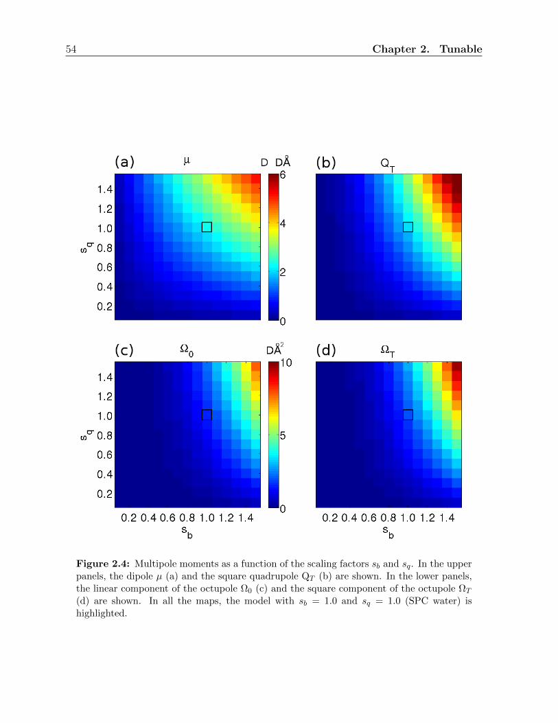
54 Chapter 2. Tunable
Figure 2.4: Multipole moments as a function of the scaling factors sb and sq. In the upperpanels, the dipole µ (a) and the square quadrupole QT (b) are shown. In the lower panels,the linear component of the octupole Ω0 (c) and the square component of the octupole ΩT
(d) are shown. In all the maps, the model with sb = 1.0 and sq = 1.0 (SPC water) ishighlighted.
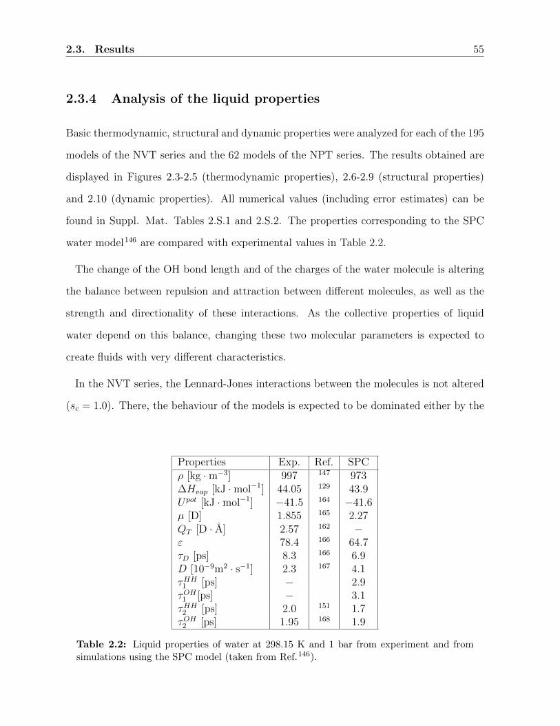
2.3. Results 55
2.3.4 Analysis of the liquid properties
Basic thermodynamic, structural and dynamic properties were analyzed for each of the 195
models of the NVT series and the 62 models of the NPT series. The results obtained are
displayed in Figures 2.3-2.5 (thermodynamic properties), 2.6-2.9 (structural properties)
and 2.10 (dynamic properties). All numerical values (including error estimates) can be
found in Suppl. Mat. Tables 2.S.1 and 2.S.2. The properties corresponding to the SPC
water model146 are compared with experimental values in Table 2.2.
The change of the OH bond length and of the charges of the water molecule is altering
the balance between repulsion and attraction between different molecules, as well as the
strength and directionality of these interactions. As the collective properties of liquid
water depend on this balance, changing these two molecular parameters is expected to
create fluids with very different characteristics.
In the NVT series, the Lennard-Jones interactions between the molecules is not altered
(sc = 1.0). There, the behaviour of the models is expected to be dominated either by the
Properties Exp. Ref. SPCρ [kg ·m−3] 997 147 973∆Hvap [kJ ·mol−1] 44.05 129 43.9Upot [kJ ·mol−1] −41.5 164 −41.6µ [D] 1.855 165 2.27QT [D · A] 2.57 162 −ε 78.4 166 64.7τD [ps] 8.3 166 6.9D [10−9m2 · s−1] 2.3 167 4.1τHH1 [ps] − 2.9τOH1 [ps] − 3.1τHH2 [ps] 2.0 151 1.7τOH2 [ps] 1.95 168 1.9
Table 2.2: Liquid properties of water at 298.15 K and 1 bar from experiment and fromsimulations using the SPC model (taken from Ref.146).

56 Chapter 2. Tunable
electrostatic interactions (high sq and sb) or the Lennard-Jones interactions (low sq and
sb). In the first case the systems will be overstructured, possibly leading to a glassy state.
Among the 195 NVT models, 41 indeed show characteristics typical for a glassy solid.
In the NPT series, the repulsion term C1/212 of the Lennard-Jones interaction function is
tuned (sc 6= 1.0) in order to obtain densities comparable to the experimental value for liquid
water. In this case the balance between electrostatics and Lennard-Jones interactions is
largely restored, and the models are expected to show characteristics closer to those of
liquid water.
In the following sections, the properties of the models of both the NVT and the NPT
series are analyzed, focusing on the trends in these properties upon variation of the scaling
factors sb and sq. Special attention is given to systems that show characteristics compatible
with a liquid. The properties of the models that are in a glassy state are only described
briefly.
Pressure P
For the NVT models, the pressure P of the systems was monitored. The results are
displayed in Figure 2.3a. The value for the model W1.01.0, which is equivalent to SPC water,
is -71 bar. The slightly negative value is due to the small discrepancy between the density
of the system simulated (968 kg m−3) and the equilibrium density146 of 973 kg m−1 for SPC
water at 1 bar). To our knowledge ,the dependence of the pressure on the density was never
systematically studied for SPC water, but values of the pressure at different densities are
reported in Ref.145, which were used for the calculation of the isothermal compressibility.
The value of -71 bar obtained here at 968 kg m−3 leads to a compressibility of 54.0 10−6
bar−1, which is compatible with the result reported for this model in Ref.145
The pressure shows a monotonic dependence upon variations of sb and sq. A decrease of

2.3. Results 57
both scaling factors is increasing the pressure (up to about 104 bar), while an increase of
both scaling factors is decreasing it (down to about −3 ·104 bar). Decreasing or increasing
one of the two scaling factors while keeping the other constant has about the same effect
irrespective of the selected scaling factor, i.e. the map in Figure 2.3a is approximately
symmetric around the diagonal. Decreasing one factor while equivalently increasing the
other one keeps the value of the pressure P approximately constant, as long as sq is not
larger than 1.2. For larger values of sq, a smaller decrease of sb is needed in order to keep
the pressure in the same range. Note that negative values of the pressure are perfectly
acceptable physically. Based on equation 2.6, they merely indicate that the virial is larger
than the kinetic energy, and that a pulling force would have to be applied to the walls of the
computational box to maintain the volume in a constant-pressure simulation. In practice,
when the pressure is very negative (P < −2 10−3 bar), the statistical error calculated
from the five different simulation repeats is larger than 100 bar (see Table 2.S.1) and the
systems are typically found in a solid (glassy) state.
Total Potential Energy U
Figures 2.3c and 2.3d show the dependence of the potential energy U on sb and sq. Note
that the scale is restricted to a range between −60 and 0 kJ·mol−1, so as to focus on the
characteristics of the liquid systems. The values of U for W1.01.0 and Y1.0
1.0 (SPC charges
and bond lengths) are -41.5 kJ·mol−1 and -43.4 kJ·mol−1, respectively. The value for the
NVT model is in line with the experimental value and the typical value for SPC water136
(see Table 2.2). The scaling of the repulsive Lennard-Jones parameter C1/212 for the NPT
model Y1.01.0 (sc = 0.9735) decreases the potential energy U by about 2 kJ·mol−1. This
effect is explained by the decreased repulsion parameter along with unaltered charges.
The Y1.01.0 water is denser than SPC water, so the potential energy is lower. The NVT
models Wsbsq show a dependence of the total potential energy U on variations of sb or sq

58 Chapter 2. Tunable
analogous to that of the pressure P . The map in Figure 2.3c is also essentially symmetric
around the diagonal. The decrease of both scaling factors simultaneously increases the
potential energy up to values close to 0 kJ·mol−1 (e.g. -3.5 to -1.5 kJ·mol−1 for the
models with scaling factor sb or sq equal to 0.1 or 0.2). The simultaneous increase of
both scaling factors decreases the potential energy U to values smaller than -60 kJ·mol−1.
These systems correspond to the models with pressure P below -1000 bar and are in a
solid (glassy) state. The lowest values of the potential energy U are around -950 kJ·mol−1.
Static Relative Dielectric Permittivity ε
Figures 2.5a and 2.5b show the variations of the dielectric permittivity ε as a function of
the two scaling factors sb and sq for the solvent of NVT and NPT series. The dielectric
permittivity was calculated only for the systems considered liquid. In the case of solids,
the fluctuations in the total dipole moment of the system lose their meaning and the
Kirkwood-Frohlich-type equation cannot be used. The value obtained for the W1.01.0 model
is 64.0 (in line with the standard value of SPC, see Table 2.2), while it increases to 68.1
for the Y1.01.0 model.
In the NVT series, the maximum value obtained for the dielectric permittivity is 140.4
for the W0.71.5 model. For the models with charges scaled by sq > 1.0 and bonds scaled
by 0.6 < sb < 1.0 (the value of sb depending on scaling of the charges), the dielectric
permittivity is larger than 65. A total of 13 NVT models have dielectric permittivities
higher than that of SPC water. Note that models with high values of both scaling factors
are solid, so that their dielectric permittivity is not considered here, meaning that the limit
sb < 1.0 for models with sq > 1.0 is due to the glassy state of those systems. Lower values
of ε, in a range from 20 to 64, are obtained for models with sq > 0.5, with a minimum
value of the scaling factor sb depending on the scaling of the charges but always larger

2.3. Results 59
Figure 2.5: Upper panel: the dielectric permittivity ε as a function of the scaling factorssb and sq for the NVT models (a) and for the NPT models (b). Lower panels: number ofthe hydrogen bonds per molecule nH as a function of the scaling factors sb and sq for theNVT models (c) and for the NPT models (d). In all the maps, the model with sb = 1.0 andsq = 1.0 (SPC water in the NVT series, closest one in the NPT series) is highlighted.

60 Chapter 2. Tunable
than 0.4. For models with sb < 0.4 or sq < 0.4, the dielectric permittivity is never higher
than 20, independently of the other scaling factor. When both scaling factors are smaller
than 0.5, ε is never higher than 2. The lowest value obtained is 1.
In the NPT series, the maximum value obtained for the dielectric permittivity is 147.5
for the Y0.71.5 model. A total of 11 models have dielectric permittivities higher than that of
SPC water, with similar combinations of sb and sq as in the NVT series. The NPT models
with high charges and short bond lengths or low charges and long bond lengths have ε
values smaller than 20. In this series, values of the dielectric permittivity lower than 7.3
cannot be found.
For both series, the dependence of the dielectric permittivity seems to be approximately
symmetric with respect to the two scaling factors when these are smaller than 1.0. For
higher factors, the behaviour is different depending on the factor that is changed. With
high charges (sq > 1.0), high values of the dielectric permittivity are obtained. Longer
bond lengths seem unable to reach the same effect.
Hydrogen-bonding Capacity nH
In Figures 2.5c and 2.5d, the average numbers of hydrogen bonds nH per molecule are
given as a measure of the hydrogen-bonding capacity of the models. The W1.01.0 model and
the Y1.01.0 have nH = 3.4 (as expected for SPC water) and nH = 3.5, respectively. In the
NVT series, 18 models have a nH value equal to 4 (all of them in the solid state). For for
the NPT series, the maximum value obtained is 3.7 (for the models Y1.10.9, Y1.2
0.8, Y1.30.7, and
Y1.40.6). All the NVT models in a solid state have nH > 3.5. Values of nH smaller than 2
can be obtained with one of the two tuned parameters scaled to low values and the whole
range of the other. The lowest values obtained are 1.4 for the NVT series and 1.7 for
the NPT series. The dependence of nH is again essentially symmetric relative to the two
2.3. Results 61
scaling factors.
Radial Distribution Function g(r)
The overall structure of the systems was analyzed by calculating the radial distribution
functions g(r). In Figure 2.6, one illustrative example is shown for each of the two solvent
series, considering the variation of the radial distribution function upon changing of the
scaling factor sb, while keeping sq = 1.0 (panels (a) and (b) of the figure, Wsb1.0 and Ysb
1.0,
respectively) or upon changing the scaling factor sq, while keeping sb = 1.0 (panels (c) and
(d) of the figure, W1.0sq and Y1.0
sq , respectively). The radial distribution functions g(r) on
the top and on the bottom panels of each graph are those of the extreme cases accepted as
liquid models. The trends in the position and height of the first g(r) peak are also shown
in Figure 2.7 for all the models of the two series.
For the NVT series and with sq = 1.0, see Figure 2.6a, the extreme values of the scaling
factor sb considered for a liquid are 1.0 (normal SPC water) and 0.1. The W1.01.0 model
shows the typical radial distribution function of SPC water. The first relatively narrow
peak is around 0.28 nm, with a height of 2.87, and the first minimum is at 0.31 nm. Also
visible are a second and a third peak, broader than the first, at 0.45 nm and 0.68 nm,
respectively. The function converges to a value of 1 in the long-distance limit. When the
scaling factor sb is decreased, the first peak becomes quickly (already for the model W0.91.0)
broader. Its height is reduced and it shifts to longer distances. A further decrease of the
scaling factor sb keeps shifting the position of the peak, up to about 0.32 nm for the W0.11.0
model, close to the distance at the minimum of the Lennard-Jones interaction function for
SPC water which is 0.35 nm. The height of this first peak initially decreases (from sb = 1.0
to 0.6) but then increases again (from sb = 0.6 to 0.1). The first minimum also becomes
broader and shifts to the position of the second peak in the g(r) of the SPC model, while

62 Chapter 2. Tunable

2.3. Results 63
Figure 2.6: [Previous page] Upper panels: radial distribution function g(r) for differentvalues of the scaling factor sb together with sq = 1.0, for NVT simulations (a) and NPTsimulations (b). In the central part, g(r) is shown in the form of stripes. The upper andlower parts show the function g(r) of W1.0
1.0 and Y1.11.0 (top), and W0.1
1.0 and Y0.61.0 (bottom).
Lower panels: radial distribution function g(r) for different values of the scaling factor sqtogether with sb = 1.0, for NVT simulations (c) and NPT simulations (d). In the centralpart, g(r) is shown in the form of stripes. The upper and lower parts show the function g(r)of W1.0
1.1 and Y1.11.0 (top), and W0.1
1.0 and Y0.61.0 (bottom).
Figure 2.7: Upper panels: position rmax of the first peak in the radial distribution functiong(r) as a function of the scaling factors sb and sq for the NVT models (a) and the NPTmodels (b). Lower panels: the height gmax of the first peak in the radial distribution functiong(r) as a function of the scaling factors sb and sq for the NVT models (c) and the NPTmodels (d). In all the maps, the model with sb = 1.0 and sq = 1.0 (SPC water in the NVTseries, closest one in the NPT series) is highlighted.
64 Chapter 2. Tunable
the second peak is now almost overlapping with the original third minimum and becomes
broader and higher.
For the NVT series and with sb = 1.0, see Figure 2.6c, the extreme values of the scaling
factor sq considered for a liquid are 1.1 and 0.1. The behaviour of the systems upon
decreasing the scaling factor sq is very similar to the one observed upon decreasing the
scaling factor sb. One observes a broadening and lowering of the first peak, followed by an
increase, along with a shifting to larger distances. Simultaneously, one sees a broadening
of the first minimum. The second and third peaks become more evident, broader and
more defined, equally shifted to larger distances. Figures 2.6a and 2.6c also show cases
characteristic of a glassy state (sq = 1.0 with sb > 1.0 or sb = 1.0 with sq > 1.1). The
general behaviour is again similar for both scaling factors. Upon increasing sb and sq,
the system becomes in this case overstructured, as a consequence of the change of state.
The first peak becomes sharper and higher, and its position is shifted, this time to lower
distances. The first minimum is lower and shifted. The second and third peaks are again
sharper and higher, and shifted to lower distances. A fourth peak appears. The increase
of the scaling factor sb shows a much more pronounced shift (for the model W1.51.0 the
position of the first minimum is 0.20 nm, compared with 0.25 nm for the model W1.01.5).
Additionally, for the models with the two largest factors sb = 1.4 and sb = 1.5, a double
first peak appears, and the following peak is destructured. This is because the system
becomes inhomogeneous, including clusters, aggregates and bubbles. This behaviour is
not seen for the largest values of the scaling factor sq, where the glassy system remains
homogeneous.
The trends observed and the considerations made for the NVT systems are essentially
valid also for the NPT series, see Figure 2.6b and 2.6d. The structure of the Y1.01.0 model is
the same as that of W1.01.0. The decrease of both sb and sq is progressively broadening the
first peak, while shifting it. The second and the third peaks start to become less defined.

2.3. Results 65
Compared to the NVT models, the decrease of the two scaling factors is not having the
effect of initially lowering and then increasing the height of the first peak. The trend in
this case shows a clear monotonic decrease.
Dipole-dipole orientation correlation function c(r)
The dipole-dipole orientation correlation function c(r) gives a measure of the alignment of
the water molecules as a function of distance. Figure 2.8 shows one illustrative example for
each of the two solvent series, considering the variation of this function upon changing the
scaling factor sb, while keeping sq = 1.0 (panels (a) and (b) of the figure, Wsb1.0 and Ysb
1.0,
respectively) and upon changing the scaling factor sq, while keeping sb = 1.0 (panels (c)
and (d) of the figure, W1.0sq and Y1.0
sq , respectively). The dipole-dipole orientation correlation
functions c(r) on the top and on the bottom panels of each graph represent the extreme
cases accepted as liquid models. The trend in the position and the height of the first c(r)
peak are also shown in Figure 2.9 for all the models of the two series.
For the NVT series with sq = 1.0, see Figure 2.8a, the extreme values of the scaling factor
sb considered for a liquid are 1.0 (normal SPC water) and 0.1. The W1.01.0 model shows the
typical dipole-dipole orientation correlation function of SPC water. The first neighbors of a
water molecule strongly favor an alignment of the dipoles with the central molecule, as seen
from the first correlation peak at 0.27 nm. The first minimum around 0.4 nm is slightly
negative and the second peak follows at around 0.5 nm. The correlation is in general
positive almost everywhere and levels off towards zero at long distances, showing the
random orientation at long range. Decreasing the scaling factor sb has initially the effect
of broadening and lowering the first peak, sign of a weaker correlation of the first neighbors.
The maximum width of the peak is reached with sb = 0.8, then it starts to become narrower
and lower, until it almost completely disappears for sb < 0.4. The position of the first

66 Chapter 2. Tunable

2.3. Results 67
Figure 2.8: Upper panels: dipole-dipole orientation function c(r) for different values ofthe scaling factor sb together with sq = 1.0, for NVT simulations (a) and NPT simulations(b). In the central part, c(r) is shown in the form of stripes. The upper and lower partsshow the function c(r) of W1.0
1.0 and Y1.11.0 (top), and W0.1
1.0 and Y0.61.0 (bottom). Lower panels:
dipole-dipole orientation function c(r) for different values of the scaling factor sq togetherwith sb = 1.0, for NVT simulations (c) and NPT simulations (d). In the central part, c(r)is shown in the form of stripes. The upper and lower parts show the function c(r) of W1.0
1.1
and Y1.11.0 (top), and W0.1
1.0 and Y0.61.0 (bottom).
Figure 2.9: [Previous page] Upper panels: position rmax of the first peak in the dipole-dipole orientation function c(r) as a function of the scaling factors sb and sq for the NVTmodels (a) and the NPT models (b). Lower panels: height cmax of the first peak in thedipole-dipole orientation function c(r) as a function of the scaling factors sb and sq for theNVT models (c) and the NPT models (d). In all the maps, the model with sb = 1.0 andsq = 1.0 (SPC water in the NVT series, closest one in the NPT series) is highlighted.

68 Chapter 2. Tunable
peak also varies upon decreasing the scaling factor, shifting to long distances following
the trend of the radial distribution function g(r), sign that the major contribution to the
dipole alignment comes from the first neighbors. Models with the lowest values for sb
completely lose the preference for a specific alignment of the dipoles (random orientation),
as expected with a decrease of the importance of the electrostatic interaction. For these
models, the Lennard-Jones contribution is dominating and the correlation of the dipole-
dipole orientation is almost zero everywhere. When the scaling factor sb is increased above
sb = 1.0, the systems become glassy. The first peak becomes narrower and higher, and
shifts to shorter distances, indicating a higher correlation between the dipoles, consequence
of the overstructuring of the models due to the transition to a solid state. A second peak
starts to be evident, increasing with the increase of the scaling factor, further sign of the
change of state. The last two models (sb = 1.4 and sb = 1.5) show in the opposite a very
peculiar behaviour. A fist negative peak appears at around 0.2 nm, followed by a second
positive peak at similar distances compared with the first peaks of the models with smaller
scaling factors. A third and a fourth peak appear, even though not very defined, following
minima again with negative values. These two models display a double first peak in the
radial distribution function g(r), corresponding to the same positions as the first negative
peaks in c(r). The following peaks and their distorted shapes indicate an inhomogeneity in
the systems. These solids are forming aggregates and clusters, with empty areas (bubbles).
A similar behaviour is seen in case of the decrease of the scaling factor sq with sb = 1.0,
see Figure 2.8c. In this case the broadening is less pronounced, as well as the shift of the
first peak to longer distances, but the essential trends are the same. When the scaling
factor sq is increased above 1.1 (glassy systems), the dipole-dipole orientation correlation
function c(r) shows at first a trend very similar to the one observed with an increase of
the scaling factor sb. The first peak becomes again narrow and higher, shifting to shorter
distances, and the second peak becomes more and more evident. The models with higher

2.3. Results 69
charges are not showing the same peculiar characteristics of the models with the longest
bond lengths. The increase of the charge values is not leading to inhomogeneity in the
system.
In the NPT series, the Lennard-Jones interactions are tuned to obtain a density close
to the experimental density of liquid water. In this case, the equilibrium between the
electrostatic and the Lennard-Jones interactions is somewhat restored. Reflecting this
balance, the dipole-dipole correlation functions of the NPT models have very similar shapes
for all the models, see Figures 2.8b and 2.8d. In particular, the position of the first peak
is in the same range (0.27-0.28 nm). The height of the first peak shows more pronounced
variations, with values that vary between 0.07 and 0.53, increasing mainly with the increase
of the scaling factor sq, and to a lower extent with the increase of the scaling factor sb. As
expected, the variation of the charges has a stronger effect on the orientation of the dipoles
in the system than that of the bond length. Additionally, it seems that the enhancement
of the Lennard-Jones interaction (less repulsive C1/212 ) is not sufficient to restore completely
the influence of the electrostatics when too small charges are used.
Self-Diffusion Coefficient D
Figures 2.10a and 2.10b show the diffusion constant D as a function of the scaling factors
sb and sq. The diffusion constant for the W1.01.0 model is 4.17·10−9 m2·s−1 (typical value
for SPC water, see Table 2.2), while the slight change in the Lennard-Jones repulsion is
decreasing the value of the Y1.01.0 model to 3.84·10−9 m2·s−1. Reducing the Lennard-Jones
repulsive term allows for the molecules to get closer and it increases the influence of the
electrostatic, making the system less diffusive.
The only 8 systems with a diffusion coefficient lower than that of SPC but still in a
reasonable liquid-like range (0.2-3.1·10−9 m2·s−1) are W1.40.6, W1.3
0.7, W1.20.8, W1.1
0.9 (models with

70 Chapter 2. Tunable
sb > 1.0 and sq < 1.0) and W1.11.0, W0.9
1.2, W0.91.3, W0.8
1.5 (models with sb < 1.0 and sq > 1.0).
Decreasing one of the two scaling factors while keeping the other constant or both factors
simultaneously has the same effect independently of which parameter is reduced. The
diffusion constant initially increases to values between 10·10−9 m2·s−1 and 11.8·10−9 m2·s−1
(for W0.81.3), but then decreases to values between 7·10−9 m2·s−1 and 10·10−9 m2·s−1. Values
lower than 7·10−9 m2·s−1, but still higher than the one of SPC water, are possible with
sb < 0.3 and sq > 1.0.
When the scaling factors are both very high, the diffusion coefficient D of the models is
decreasing to values close to zero. This, combined with the considerations on the properties
analyzed before, confirms that these systems are in a solid (glassy) state.
For the NPT series, the behaviour is similar. In this case, models with both scaling
factors simultaneously very low or very high were not feasible. The decrease of one of
the two scaling factor while keeping the other constant or of both factors simultaneously
increases the diffusion constant, initially to values between 10·10−9 m2·s−1 and 15·10−9
m2·s−1, and further up to 20·10−9 m2·s−1. A further decrease seems to evidence a lowering
of the diffusion constant similar to the NVT models.
Rotational Correlation Time τOH2
Two different rotational correlation times were calculated, namely τOH2 corresponding to
the OH vector along the bonds of the molecules and τHH2 corresponding to the vector HH
connecting the two hydrogen atoms. Only τOH2 is displayed in Figures 2.10c and 2.10d
and will be discussed here. The other correlation time τHH2 presents similar trends (data
not shown).
The value of τOH2 for the W1.01.0 model is 1.4 ps, lower than what is found in the literature
for SPC water (see Table 2.2). The Y1.01.0 model shows a rotational correlation time of 1.8

2.3. Results 71
Figure 2.10: Upper panels: the diffusion constant D as a function of the scaling factorssb and sq for the NVT models (a) and the NPT models (b). Central panel: the rotationalcorrelation time τOH2 as a function of the scaling factors sb and sq for the NVT models (c)and the NPT models (d). Lower panels: the Debye relaxation time τD as a function of thescaling factors sb and sq for the NVT models (e) and the NPT models (f). In all the maps,the model with sb = 1.0 and sq = 1.0 (SPC water in the NVT series, closest one in the NPTseries) is highlighted.

72 Chapter 2. Tunable
ps. In the NVT series, an increase of the scaling factors is immediately increasing the
rotational time. In some cases, the autocorrelation function is not decorrelating to 0 even
after nanoseconds. When this happens, the rotational time is reported as > 21 ns. This
behaviour is in line with the other properties calculated, giving further confirmation of
the change of state of these models. For the other models which remain liquid, three cases
can be found. In the first case, the autocorrelation function is relaxing so fast that it is
already close to zero within 0.2 ps or less and assumes immediately a damped oscillatory
behaviour. For these systems, the rotational correlation time is reported as τ < 0.2 ps.
In the second case, 5 models have a rotational correlation time longer than SPC water,
namely W1.40.6 (3.9 ps), W1.3
0.7 (3.7 ps), W1.20.8 (2.7 ps), W1.0
1.1 (12.6 ps) and W0.81.5 (3.6 ps). These
models show a diffusion constant similar to the one of SPC water. In the third case,
models have a rotational correlation time shorter than SPC water.
A very similar behaviour is observed for the NPT series, with the NPT models corres-
ponding to a given NVT model having similar characteristics. For this series, the slowest
model has a rotational correlation time of 5.1 ps (Y1.20.8), still much shorter than the slowest
NVT model (12.6 ps).
Note that the values of the rotational times are affected by very high statistical uncertain-
ties, in particular because the fitting procedure of the autocorrelation function is prone
to depend on arbitrary choices. For example, a change in the time interval considered
for the exponential fit, keeping the same criterion for the coefficient of determination
(R2 > 0.9), can yield a variation in the rotational time of up to 50%. For this reason, the
values reported for the rotational times have to be considered indicative and the trends
qualitative.

2.3. Results 73
Debye Relaxation Time τD
Figures 2.10e and 2.10f show the Debye relaxation time as a function of the scaling factors
sb and sq. The value for the W1.01.0 model is lower than expected for SPC water (5.1 ps
instead of 6 ps). Also the value for the unmodified NPT model Y1.01.0 is lower than the one
of SPC water (5.6 ps instead of 6 ps). The Debye relaxation times shorter than 1 ps were
not considered. In the NVT series, the same 5 models that evidenced a rotational time
longer than SPC water, plus two additional ones (W0.91.1 and W0.8
1.4), have a Debye relaxation
time longer than that of SPC water. The slowest model has a relaxation time of 24.7 ps
(W0.81.5). In the NPT series, the corresponding combinations of scaling factors sb and sq
(the ones that led to feasible models) show the same slowed dynamics. In this case, the
slowest model has a relaxation time of 15.2 ps (Y1.20.8).
The same considerations made in the context of the rotational correlation times (previous
section) are valid also for the Debye relaxation time. This is understandable as the latter
relaxation is a collective variant of the former single-molecule one.
The analysis of the dynamic properties of the systems confirms what is suggested by
the thermodynamic and structural analysis. In the NVT series, 41 models (large scaling
factors sb and sq) are solid. Additionally, the dynamic properties show that the NVT
models with scaling factors sb and sq smaller than 1.0 are faster than SPC water, in terms
of both translational and rotational diffusion.
State of the systems
Considering the analysis of all the properties, it is clear that, when one of the two scaling
factors is varied (modification of bond length or charges of the model), the balance between
electrostatic interaction and Lennard-Jones repulsion that is responsible for the properties
of water is disrupted.

74 Chapter 2. Tunable
A small reduction of either charges or bond lengths (sq or sb between 0.5 and 1.0) shift
the equilibrium in favor of the Lennard-Jones repulsion, destructuring the systems. The
effect is consistent for all properties. When these models are parametrized to have the same
density as water in the NPT series, the Lennard-Jones repulsion has to be reduced (sc <
1.0), restoring the balance to a large extent. With a further reduction of the scaling factors
(sq or sb smaller than 0.5), the system is completely dominated by the Lennard-Jones
interactions and becomes a more structured. These Lennard-Jones liquid-like systems
have high pressure, higher potential energy, a diffusion constant between 5·10−9 m2s−1
and 10·10−9 m2s−1 and very short rotational correlation times. When tentatively adjusted
to the NPT series, these kind of models have a density higher than that of water, so that it
is not possible to find an appropriate scaling factor sc to tune the Lennard-Jones repulsion
term for achieving the experimental density of liquid water.
An increase of the scaling factors sb and sq overstructures the systems, leading to a
change of state from liquid to solid. In this case the electrostatic interactions become
predominant. Increasing sq generates a more homogeneous structure, whereas increasing
of sb creates a more disordered and inhomogeneous state. Also in this case, tuning the
Lennard-Jones repulsive term is not successfully reproducing the density of a liquid water-
like system.
2.3.5 Correlation between the properties
The linear correlation between the different properties analyzed in the previous sections is
displayed in Figure 2.11a as a correlation matrix involving all the possible pairwise com-
binations. Dark red is indicative of a strong linear correlation, dark blue of a strong linear
anti-correlation, while colors in the range yellow-green indicate no correlation between the
properties. As linear correlation is only one possible type of correlation, correlation plots

2.3. Results 75
for specific pairs of properties are also explicitly shown in Figure 2.11b.
Most of the properties turn out to be either highly linearly correlated or highly linearly
anti-correlated with each others. The most remarkable features are the following:
• A strong correlation of pressure P and total potential energy U , along with strong
correlation or anticorrelation between these two properties and all the others (except
D).
• A strong correlation of the dielectric permittivity ε with the dipole moment µ and,
to a lesser extent, the quadrupole moment QT .
• A strong correlation of the hydrogen-bonding capacity nH with the dipole moment µ
and, to a larger extent the square quadrupole moment QT and the square component
of the octupole moment ΩT .
• A relatively low correlation (0.74) between dielectric permittivity ε and the hydrogen-
bonding capacity nH .
• A relatively low correlation (below 0.65) of the dynamic properties (diffusion coef-
ficient D, rotational correlation time τOH2 and the Debye relaxation time τD) with
the other properties.
The correlation or anticorrelation of the thermodynamic properties P and U with the
others is not entirely surprising. These properties define the state of the system and the
interactions governing its behaviour. The correlation of the hydrogen-bonding capacity
with the higher-order multipoles can explain some interesting characteristics of water and
their dependence on the model as reported in literature, e.g. the dependence of the freezing
point of different water models on their quadrupole moment160.
The relatively low correlation between dielectric permittivity ε and the hydrogen-bonding
capacity nH is an interesting and useful observation concerning these water-like artificial

76 Chapter 2. Tunable
(a)
(b)

2.3. Results 77
models. It offers the possibility to engineer models with almost uncorrelated values of
the two properties, allowing for studies on the influence of the polarity of the solvent which
can disentangle of the two aspects
The behaviour of the diffusion coefficient D is somewhat anomalous, seeming not to
correlate with any of the other properties, except for a weak anticorrelation with the ro-
tational correlation time τOH2 and the Debye relaxation time τD. A closer look at this
property (Figure 2.11b) shows that the diffusion coefficient analyzed as a function e.g.
of the hydrogen-bonding capacity nH or the total potential energy U displays a double
regime. This is easily explained based on the above considerations concerning the state of
the systems. The first regime, characterized by an anticorrelation with nH at high values
of nH and a correlation with U at low values of U , corresponds to systems for which either
the charges or the bond lengths are slightly reduced. For these models the electrostatic
interactions are less important than for normal SPC water. The second regime, char-
acterized by opposite correlations between diffusion coefficient D and hydrogen-bonding
capacity nH or total potential energy U , includes models that behave like Lennard-Jones
liquids. The turning point is given by the maximum in the diffusion coefficient (about 12
Figure 2.11: [Previous page] (a) Linear correlation matrix obtained considering all possiblepairwise combinations of the calculated properties. The properties are the dipole µ, thesquare component of the quadrupole QT , the square component of the octupole ΩT , thelinear component of the octupole Ω0, the dielectric permittivity ε, the hydrogen-bondingcapacity nH , the pressure P , the total potential energy per molecule U , the self-diffusionconstant D, the rotational correlation time for the OH vector τOH2 and the Debye relaxationtime τD. The correlation coefficients are calculated as Pearson’s coefficient (see Section2.2.6). For the NVT solvents series, only models that are in a liquid state are considered. Acorresponding correlation matrix for the NPT models is given in Figure 2.12. (b) Correlationplots for specific pairs of properties considered. The hydrogen-bonding capacity nH (firstrow from the top) is displayed as a function of all the multipole moments. The dielectricpermittivity ε is displayed as a function of µ, P , U or nH . The pressure P is displayed asa function of µ, QT , ΩT or U . The diffusion coefficient D is displayed as a function of Ω0,nH , U or τD. For each plot, the value of the corresponding linear correlation coefficient isalso indicated.

78 Chapter 2. Tunable
10−9 m2·s−1).
Figure 2.12: Linear correlation matrix obtained considering all possible pairwise combin-ations of the calculated properties for the NPT models. The properties are the dipole µ,the square component of the quadrupole QT , the square component of the octupole ΩT , thelinear component of the octupole Ω0, the dielectric permittivity ε, the hydrogen-bondingcapacity nH , the total potential energy per molecule U , the self-diffusion constant D, therotational correlation time for the OH vector τOH2 , the Debye relaxation time τD and thescaling factor sc. The correlation coefficients are calculated as Pearson’s coefficient (seeSection 2.2.6).

2.3. Results 79
2.3.6 Solvation free energy
In Figure 2.13, The solvation free energy of argon, water and a sodium ion is shown as
a function of the solvents considered in the four series described in Section 2.2.7. In
the figure, the main properties of the solvents, dielectric permittivity, hydrogen-bonding
capacity and scaling factor sc, are displayed in the first and the second panel of the figure
from the top. The values are also reported in Table 2.1.
The results for the corresponding simulations in SPC water (horizontal dashed line in
the panels) show that the sodium ion Na+ (third panel from bottom) is highly soluble in
water (highly negative free energy). For this species, the interaction with the solvent is
entirely dominated by the electrostatic interactions. The variation in the free energy of
solvation along the four series of solvents considered is strongly dependent on the variation
of the dielectric permittivity of the solvent, even in the two series SPh and Sph, for which
the hydrogen-bonding capacity is varied. The reduction of ε is increasing the ∆F , making
the compound less soluble.
In the opposite, argon Ar (top panel) is poorly soluble in water (positive free energy).
Here, the solvation free energy is completely correlated with the change in the scaling
factor sc that is adjusting the Lennard-Jones repulsion. The solvation free energy varies
following the variation of the scaling factor sc, in particular for the series Shp and Sph. A
decrease in the Lennard-Jones repulsion (smaller sc) decreases the free energy of solvation
of the hydrophobic compound, making it less insoluble.
Water (middle panel between top and bottom) is a soluble molecule, even if the free
energy value in this case is less negative than the one for the ionic species. A decrease of
the permittivity of the solvent at hydrogen-bonding capacity similar to water is decreasing
the solvation free energy of this molecule, as does a decrease in the hydrogen-bonding
capacity at a permittivity similar to the one of water. When one of the two properties

80 Chapter 2. Tunable
is reduced, a variation of the other does not have a large influence on the solvation free
energy of this species. Water solvation appears to be a cooperation between the specific
H-bond network and the permittivity of the solvent.
Figure 2.13: Solvation free energy of three species in artificial solvents of the NPT seriesat 298.15 K and 1 bar. The values are calculated from the progressive perturbation ofthe solute into a dummy atom using thermodynamic integration. The three compoundsconsidered are (from top to bottom) argon Ar, SPC water H2O and sodium ion Na+. Thepoints follow the four series of artificial solvents (Table 2.1) SHp , Shp , SPh and Sph. The valuesof the solvent permittivity ε (orange, scale on the left) and hydrogen-bonding capacity nH(blue, scale on the right) are also displayed (top row), together with the scaling factor sccontrolling the Lennard-Jones repulsive term.

2.4. Conclusions 81
2.4 Conclusions
In the present work, we have considered a wide spectrum of water-like models derived from
SPC water model136 with altered geometries (OH bond distance) and dipole moments (O
and H charges), but approximately the same molecular size (same or similar Lennard-
Jones interaction parameters). Their simulated properties have been investigated in details
in order to examine the influence of the altered molecular parameters on the collective
properties of the liquid.
In the NVT series, the Lennard-Jones interaction parameters were kept identical to those
of SPC water and the pressure in the system may significantly differ from the atmospheric
pressure. In the NPT series, the Lennard-Jones repulsion was adjusted to reproduce
densities similar to normal SPC water at room temperature and atmospheric pressure.
The analysis of the properties of these models illustrates the delicate balance between
electrostatic and Lennard-Jones interactions responsible of the very particular properties
of water. A decrease in the bond length or/and partial charges of the model reduces the im-
portance of the electrostatic interaction, leading to models that behave like Lennard-Jones
fluids. In the opposite, an increase in the bond length or/and partial charges overstructures
the system, yielding models that ultimately adopt a glassy state.
The analysis of the correlations between the properties analyzed leads to interesting
insight about the nature of certain characteristics of water. In particular, the dielec-
tric permittivity seems to mainly depend on the dipole moment of the model, while the
hydrogen-bonding capacity is more connected to higher order multipoles, in particular
the quadrupole and the octupole. Additionally the correlation of the dynamic properties
(diffusion coefficient D, rotational correlation time τOH2 and the Debye relaxation time τD)
can be used to characterize the two different type of behaviors of the models described
before.
82 Chapter 2. Tunable
The low correlation between dielectric permittivity and hydrogen-bonding capacity of
these models allows for their use as liquid environment in studies concerning the effect of
the polarity of the solvent on a solute, giving the possibility to analyze (almost) separately
the influence of these two characteristics. A simple example of this is provided here with
the calculation of the solvation free energy of three different chemical species as a function
of the dielectric permittivity and of the hydrogen-bonding capacity of the solvent. It was
possible to qualitatively determine the importance of the electrostatic interactions, and
more specifically of the dielectric permittivity, for ionic solvation, and of the Lennard-
Jones interactions for a hydrophobic compound. The interplay between these two aspect
of the polarity of the solvent was highlighted in the determination of the solvation free
energy of water.
More extensive studies on the conformational properties of saccharides (monomers and
dimers) using these artificial water-like models are described in the following chapters of
this thesis.

2.A. Multipoles 83
2.A Multipoles
In this appendix, we derive Eq. 2.1-2.5 concerning the multipole moments of a molecule
with three atomic sites (SPC-like geometry). A discrete distribution of N point charges
ql at positions rl in vacuum is considered. The electric potential Φ(R) generated by this
distribution at position R from an origin O, chosen close to the center of mass of the
distribution, is given by the Coulomb potential
Φ(R) =1
4πε0
N∑l=1
ql||R− rl||
, (A.2.1)
where ε0 is the dielectric permittivity in vacuum.
This expression can be expanded as a Taylor series considering distances R from the
origin O that are larger than the maximum distance R0 between the charges, i.e. when
R >> R0 with R = ||R|| and R0 = max(||rl||), as
Φ(R) =1
4πε0
(1
Rq +
1
R2
∑i=x,y,z
Riµi +∑
i,j=x,y,z
RiRjQi,j (A.2.2)
+1
6
1
R4
∑i,j,k=x,y,z
RiRjRkOi,j,k + · · ·
)(A.2.3)
where

84 Chapter 2. Tunable
q =N∑l=1
ql (A.2.4)
µi =N∑l=1
qlrl,i (A.2.5)
Qi,j =1
2
N∑l=1
ql(3rl,irl,j − r2l δij) (A.2.6)
Oi,j,k =N∑l=1
(15rl,irl,jrl,k − 3r2l (rl,iδjk + rl,jδik + rl,kδi,j)) (A.2.7)
are the total charge q of the system, the elements µi of the dipole vector, the elements Qi,j
of the traceless quadrupole tensor Qij and the elements Oi,j,k of the octupole tensor Ωijk.
The index l refers to the individual charges, while the indices i, j, k refer to the x, y, z
components of tensors. The whole formalism can also be generalized to a continuous
distribution.
Let us consider a water molecule described by the SPC model136 (see Figure 2.1). The
charges are distributed on the oxygen (−2q) and on the two hydrogens (q). The distances
between them are given by the bond length b (dOH) and by 2b sinα (dHH), where α = θ/2
is half of the angle HOH. A coordinate system is defined with the origin O on the oxygen
atom, the xz plane corresponding to the molecule plane, the z-axis on the bisector of the
bond angle, and the y axis normal to the molecular plane. In this case the total charge of
the system is zero, the molecule being neutral by construction.
The dipole vector µi, the traceless quadrupole tensor Qij and the traceless octupole
tensor Ωijk can be written in their matrix form. The dipole vector µi has one non zero
element
µi = ( 0 0 2qrH,z ) = ( 0 0 2qb cosα ) (A.2.8)
2.A. Multipoles 85
The non-zero elements of the quadrupole tensor Qij are the diagonal elements
Qij =
Qxx 0 0
0 Qyy 0
0 0 Qzz
(A.2.9)
with Qxx = q(2r2H,x− r2
H,z), Qyy = q(−r2H,x− r2
H,z) and Qzz = q(−r2H,x + 2r2
H,z). The tensor
is traceless, Qxx +Qyy +Qzz = 0.
An equivalent alternative form of the quadrupole tensor
Qij =
QT −Q0 0 0
0 −QT −Q0 0
0 0 2Q0
(A.2.10)
where QT = (Qxx − Qyy)/2 and Q0 = Qzz/2, can be written using the linear component
Q0 and the square component QT of the quadrupole tensor. An origin O′ for which the
linear component of the quadrupole is equal to zero (2Q0 = Qzz = 0) can be chosen. In
this way the quadrupole tensor is expressed just by one component, the square component
QT , defined as
QT =3
2qr2H,x =
3
2qb2sin2α. (A.2.11)
It is clear that the square component QT of the quadrupole is independent of the choice
of the origin O of coordinate and it can be used univocally to describe the strength of the
quadrupole interactions.
The non-zero elements of the octupole tensor Ωijk are
86 Chapter 2. Tunable
[Ω]ijx =
0 0 Oxzx
0 0 0
Ozxx 0 0
, (A.2.12)
[Ω]ijy =
0 0 0
0 0 Oyzy
0 Ozyy 0
, (A.2.13)
[Ω]ijz =
Oxxz 0 0
0 Oyyz 0
0 0 Ozzz
, (A.2.14)
where Oxzx = Ozxx = Oxxz = q(4r2H,xrH,z−r3
H,z), Oyzy = Ozyy = Oyyz = −q(r3H,z+r2
H,xrH,z)
and Ozzz = q(2r3H,z − 3r2
H,xrH,z).
As for the quadrupole, an alternative equivalent form can be written using the linear
component Ω0 and a square component ΩT of the octupole tensor
[Ω]ijx =
0 0 ΩT − Ω0/2
0 0 0
ΩT − Ω0/2 0 0
, (A.2.15)
[Ω]ijy =
0 0 0
0 0 −ΩT − Ω0/2
0 −ΩT − Ω0/2 0
, (A.2.16)

2.A. Multipoles 87
[Ω]ijz =
ΩT − Ω0/2 0 0
0 −ΩT − Ω0/2 0
0 0 Ω0
, (A.2.17)
In this way only two components are necessary to describe the octupole interactions, the
linear component of the octupole tensor Ω0, defined as
Ω0 = q(2r3H,z − 3r2
H,xrH,z) = 2b3cosα(2sin2α− 3cos2α) (A.2.18)
and the square component ΩT , defined as
ΩT =5
2qr2H,xrH,z =
5
2qb3sin2αcosα. (A.2.19)

88 Chapter 2. Tunable
2.S.1 Supplementary Material

2.S.1. Supplementary Material 89
Table
2.S.1:
Sim
ula
ted
pro
per
ies
ofth
ew
ater
-lik
em
od
els
ofth
eN
VT
seri
esat
298.1
5K
and
ad
ensi
tyof
968
kg·m−
3.
For
each
mod
el,
the
stat
eof
the
syst
em(S
.)is
ind
icat
edas
L(l
iqu
id)
orS
(sol
id).
Th
equ
anti
ties
rep
orte
dar
eth
esc
alin
gfa
ctor
for
the
bon
dle
ngth
s b,
the
scal
ing
fact
orfo
rth
ep
arti
alch
arge
ss q
,th
ed
ipol
em
omen
tµ
ofth
em
od
el,
the
squ
are
com
pon
entQT
ofth
equ
adru
pol
e,th
eli
nea
rco
mp
onen
tΩ
0of
the
oct
up
ole,
the
squ
are
com
pon
ent
ΩT
ofth
eoct
up
ole,
the
pre
ssu
reP
,th
eto
tal
pot
enti
alen
ergy
U,
the
self
-d
iffu
sion
con
stan
tD
,th
ero
tati
onal
corr
elat
ion
tim
eτOH
2fo
rth
eO
Hax
is,
the
rota
tion
al
corr
elat
ion
tim
eτHH
2fo
rth
eO
Hax
is,
the
Deb
yere
laxat
ion
tim
eτ D
,th
ep
osit
ionr m
ax
an
dth
eh
eigh
tg m
ax
ofth
efirs
tp
eak
ofth
era
dia
ld
istr
ibu
tion
fun
ctio
ng(r
),th
ep
osit
ionr m
ax
and
the
hei
ghtc m
ax
ofth
efi
rst
pea
kof
the
dip
ole-
dip
ole
orie
nta
tion
fun
ctio
nc(r)
,th
est
ati
cre
lati
ved
iele
ctri
cp
erm
itti
vit
yε
and
the
hyd
roge
n-b
ond
ing
cap
acit
ynH
.T
he
qu
anti
tiesP
,U
,D
,τ D
,ε
andnH
are
rep
orte
dw
ith
ast
atis
tica
ler
ror
(bet
wee
np
aren
thes
is)
calc
ula
ted
as
thro
ot-m
ean
-squ
are
dev
iati
onov
erfi
vere
pea
tsof
the
sim
ula
tion
s.T
he
mod
els
that
wer
en
otfe
asib
lear
en
otre
por
ted
,a
bla
nk
lin
eis
den
otin
gon
eor
mor
em
issi
ng
com
bin
atio
ns
of
scal
ing
fact
ors.
S.
s bs q
µQT
Ω0
ΩT
PU
DτOH
2τHH
2τ D
r max
(gmax)r m
ax
(cmax)
εnH
[D]
[D·A
][D·A
2]
[D·A
2]
[bar]
[kJ·m
ol−
1]
[10−9m
2s−
1]
[ps]
[ps]
[ps]
[nm
](-
)[n
m]
(-)
W0.1
0.9
L0.1
0.9
0.2
0.0
0.0
00.0
010183.7
(6.5
)-1
.8(0
.0)
8.3
(0.2
)<
0.2
<0.2
1.0
(0.0
)0.3
1(2
.46)
0.3
1(0
.00)
1.1
(0.0
)1.4
(0.0
)
W0.1
1.0
L0.1
1.0
0.2
0.0
0.0
00.0
07797.2
(3898.6
)-1
.5(0
.8)
6.1
(3.0
)<
0.2
<0.2
1.0
(0.0
)0.3
2(2
.49)
0.3
1(0
.00)
1.2
(0.0
)1.4
(0.1
)
W0.1
1.1
L0.1
1.1
0.2
0.0
0.0
00.0
09131.3
(15.4
)-2
.1(0
.0)
6.8
(0.1
)<
0.2
<0.2
1.0
(0.0
)0.3
2(2
.54)
0.3
2(0
.00)
1.2
(0.0
)1.4
(0.0
)
W0.2
0.4
S0.2
0.4
0.2
0.0
-0.0
00.0
17743.0
(3871.5
)-1
.6(0
.8)
5.9
(2.9
)>
21·1
03>
21·1
03>
21·1
03
(0.0
0)
0.3
2(2
.50)
0.3
3(0
.0)
-1.4
(0.0
)
W0.2
0.5
L0.2
0.5
0.2
0.0
-0.0
00.0
19656.2
(3.9
)-2
.0(0
.0)
7.6
(0.1
)<
0.2
<0.2
1.0
(0.0
)0.3
2(2
.50)
0.3
1(0
.00)
1.2
(0.0
)1.4
(0.0
)
W0.2
0.6
L0.2
0.6
0.3
0.0
-0.0
00.0
19601.5
(2.6
)-2
.0(0
.0)
7.5
(0.4
)<
0.2
<0.2
1.0
(0.0
)0.3
2(2
.50)
0.3
2(0
.00)
1.3
(0.0
)1.4
(0.0
)
W0.2
0.7
L0.2
0.7
0.3
0.1
-0.0
10.0
19514.0
(3.8
)-2
.0(0
.0)
7.5
(0.2
)<
0.2
<0.2
1.0
(0.0
)0.3
2(2
.50)
0.3
1(0
.00)
1.4
(0.0
)1.4
(0.0
)
W0.2
0.8
L0.2
0.8
0.4
0.1
-0.0
10.0
19363.2
(4.4
)-2
.1(0
.0)
7.2
(0.1
)<
0.2
<0.2
1.0
(0.0
)0.3
2(2
.52)
0.3
1(0
.00)
1.5
(0.0
)1.4
(0.0
)
W0.2
0.9
L0.2
0.9
0.4
0.1
-0.0
10.0
19152.9
(2.6
)-2
.2(0
.0)
6.9
(0.2
)<
0.2
<0.2
1.0
(0.0
)0.3
2(2
.53)
0.3
1(0
.01)
1.6
(0.0
)1.4
(0.0
)
W0.2
1.0
L0.2
1.0
0.5
0.1
-0.0
10.0
18865.3
(8.6
)-2
.3(0
.0)
6.3
(0.2
)<
0.2
<0.2
1.0
(0.0
)0.3
2(2
.55)
0.3
1(0
.01)
1.8
(0.0
)1.4
(0.0
)
W0.2
1.1
L0.2
1.1
0.5
0.1
-0.0
10.0
28521.6
(6.2
)-2
.5(0
.0)
6.0
(0.2
)<
0.2
<0.2
1.0
(0.0
)0.3
2(2
.58)
0.3
1(0
.01)
2.0
(0.0
)1.4
(0.0
)
W0.2
1.2
L0.2
1.2
0.5
0.1
-0.0
10.0
28140.7
(5.0
)-2
.7(0
.0)
5.6
(0.2
)<
0.2
<0.2
1.0
(0.0
)0.3
2(2
.61)
0.3
1(0
.01)
2.3
(0.0
)1.4
(0.0
)
W0.2
1.3
L0.2
1.3
0.6
0.1
-0.0
10.0
27750.3
(6.7
)-2
.9(0
.0)
5.2
(0.1
)<
0.2
<0.2
1.0
(0.0
)0.3
2(2
.65)
0.3
1(0
.01)
2.5
(0.0
)1.4
(0.0
)
W0.2
1.4
L0.2
1.4
0.6
0.1
-0.0
10.0
27380.0
(1.8
)-3
.1(0
.0)
4.9
(0.1
)<
0.2
<0.2
1.0
(0.0
)0.3
2(2
.68)
0.3
1(0
.02)
2.8
(0.0
)1.4
(0.0
)
W0.2
1.5
L0.2
1.5
0.7
0.1
-0.0
10.0
27045.5
(2.9
)-3
.3(0
.0)
4.5
(0.1
)<
0.2
<0.2
1.0
(0.0
)0.3
2(2
.72)
0.3
1(0
.02)
3.2
(0.0
)1.4
(0.0
)
W0.3
0.3
L0.3
0.3
0.2
0.1
-0.0
10.0
19735.5
(5.6
)-1
.9(0
.0)
7.5
(0.2
)<
0.2
<0.2
1.0
(0.0
)0.3
2(2
.49)
0.3
2(0
.00)
1.1
(0.0
)1.4
(0.0
)
W0.3
0.4
L0.3
0.4
0.3
0.1
-0.0
10.0
29726.7
(4.5
)-2
.0(0
.0)
7.5
(0.3
)<
0.2
<0.2
1.0
(0.0
)0.3
2(2
.49)
0.3
1(0
.00)
1.3
(0.0
)1.4
(0.0
)
W0.3
0.5
L0.3
0.5
0.3
0.1
-0.0
20.0
29703.8
(2.4
)-2
.0(0
.0)
7.7
(0.1
)<
0.2
<0.2
1.0
(0.0
)0.3
2(2
.49)
0.3
1(0
.00)
1.4
(0.0
)1.4
(0.0
)
Conti
nu
edon
Nex
tP
age.
..

90 Chapter 2. Tunable
Tab
le2.S
.1–
Conti
nu
ed
St.
s bs q
µQT
Ω0
ΩT
PU
DτOH
2τHH
2τ D
r max
(gmax)r m
ax
(cmax)
εnH
[D]
[D·A
][D·A
2]
[D·A
2]
[bar]
[kJ·m
ol−
1]
[10−9m
2s−
1]
[ps]
[ps]
[ps]
[nm
](-
)[n
m]
(-)
W0.3
0.6
L0.3
0.6
0.4
0.1
-0.0
20.0
39652.1
(2.6
)-2
.0(0
.0)
7.4
(0.1
)<
0.2
<0.2
1.0
(0.0
)0.3
1(2
.49)
0.3
1(0
.01)
1.6
(0.0
)1.4
(0.0
)
W0.3
0.7
L0.3
0.7
0.5
0.1
-0.0
30.0
49573.4
(2.0
)-2
.1(0
.0)
7.4
(0.2
)<
0.2
<0.2
1.0
(0.0
)0.3
1(2
.49)
0.3
1(0
.01)
1.9
(0.0
)1.4
(0.0
)
W0.3
0.8
L0.3
0.8
0.5
0.1
-0.0
30.0
49458.3
(1.3
)-2
.3(0
.0)
7.6
(0.3
)<
0.2
<0.2
1.0
(0.0
)0.3
2(2
.50)
0.3
1(0
.02)
2.3
(0.0
)1.4
(0.0
)
W0.3
0.9
L0.3
0.9
0.6
0.2
-0.0
30.0
49306.5
(2.0
)-2
.5(0
.0)
7.5
(0.2
)<
0.2
<0.2
1.0
(0.0
)0.3
2(2
.51)
0.3
1(0
.02)
2.7
(0.0
)1.4
(0.0
)
W0.3
1.0
L0.3
1.0
0.7
0.2
-0.0
40.0
59127.8
(1.5
)-2
.7(0
.0)
7.3
(0.2
)<
0.2
<0.2
1.0
(0.0
)0.3
2(2
.51)
0.3
1(0
.03)
3.2
(0.0
)1.4
(0.0
)
W0.3
1.1
L0.3
1.1
0.7
0.2
-0.0
40.0
68937.3
(4.3
)-3
.0(0
.0)
6.9
(0.1
)<
0.2
<0.2
1.0
(0.0
)0.3
2(2
.52)
0.3
1(0
.04)
3.8
(0.0
)1.5
(0.0
)
W0.3
1.2
L0.3
1.2
0.8
0.2
-0.0
50.0
68729.6
(1.8
)-3
.3(0
.0)
7.0
(0.2
)<
0.2
<0.2
1.0
(0.0
)0.3
2(2
.52)
0.3
1(0
.05)
4.6
(0.0
)1.4
(0.0
)
W0.3
1.3
L0.3
1.3
0.9
0.2
-0.0
50.0
78513.7
(1.2
)-3
.6(0
.0)
7.0
(0.1
)<
0.2
<0.2
1.0
(0.0
)0.3
2(2
.52)
0.3
1(0
.06)
5.5
(0.0
)1.5
(0.0
)
W0.3
1.4
L0.3
1.4
1.0
0.2
-0.0
60.0
78296.2
(3.1
)-4
.0(0
.0)
7.1
(0.1
)<
0.2
<0.2
1.0
(0.0
)0.3
2(2
.53)
0.3
1(0
.07)
6.5
(0.0
)1.5
(0.0
)
W0.3
1.5
L0.3
1.5
1.0
0.3
-0.0
60.0
78074.1
(1.8
)-4
.5(0
.0)
6.9
(0.1
)<
0.2
<0.2
1.0
(0.0
)0.3
1(2
.52)
0.3
1(0
.09)
7.7
(0.1
)1.5
(0.0
)
W0.4
0.2
L0.4
0.2
0.2
0.1
-0.0
10.0
29765.1
(4.3
)-1
.9(0
.0)
7.5
(0.1
)<
0.2
<0.2
1.0
(0.0
)0.3
2(2
.49)
0.3
1(0
.00)
1.1
(0.0
)1.4
(0.0
)
W0.4
0.3
L0.4
0.3
0.3
0.1
-0.0
30.0
49759.1
(4.5
)-1
.9(0
.0)
7.6
(0.3
)<
0.2
<0.2
1.0
(0.0
)0.3
2(2
.48)
0.3
1(0
.00)
1.3
(0.0
)1.4
(0.0
)
W0.4
0.4
L0.4
0.4
0.4
0.1
-0.0
40.0
59735.1
(2.5
)-2
.0(0
.0)
7.8
(0.2
)<
0.2
<0.2
1.0
(0.0
)0.3
2(2
.49)
0.3
1(0
.00)
1.5
(0.0
)1.4
(0.0
)
W0.4
0.5
L0.4
0.5
0.5
0.2
-0.0
40.0
69685.7
(3.0
)-2
.1(0
.0)
7.6
(0.2
)<
0.2
<0.2
1.0
(0.0
)0.3
2(2
.49)
0.3
1(0
.01)
1.8
(0.0
)1.4
(0.0
)
W0.4
0.6
L0.4
0.6
0.5
0.2
-0.0
60.0
79603.7
(2.6
)-2
.2(0
.0)
7.7
(0.2
)<
0.2
<0.2
1.0
(0.0
)0.3
2(2
.49)
0.3
1(0
.02)
2.3
(0.0
)1.4
(0.0
)
W0.4
0.7
L0.4
0.7
0.6
0.2
-0.0
70.0
89477.1
(2.3
)-2
.5(0
.0)
7.7
(0.1
)<
0.2
<0.2
1.0
(0.0
)0.3
2(2
.49)
0.3
1(0
.03)
2.9
(0.0
)1.4
(0.0
)
W0.4
0.8
L0.4
0.8
0.7
0.3
-0.0
70.1
09311.2
(1.7
)-2
.8(0
.0)
7.8
(0.2
)<
0.2
<0.2
1.0
(0.0
)0.3
2(2
.48)
0.3
1(0
.04)
3.7
(0.0
)1.5
(0.0
)
W0.4
0.9
L0.4
0.9
0.8
0.3
-0.0
90.1
19111.0
(1.9
)-3
.2(0
.0)
7.8
(0.1
)<
0.2
<0.2
1.0
(0.0
)0.3
2(2
.49)
0.3
1(0
.05)
4.7
(0.0
)1.5
(0.0
)
W0.4
1.0
L0.4
1.0
0.9
0.3
-0.1
00.1
28879.0
(0.5
)-3
.7(0
.0)
7.8
(0.1
)<
0.2
<0.2
1.0
(0.0
)0.3
2(2
.49)
0.3
1(0
.07)
5.9
(0.0
)1.5
(0.0
)
W0.4
1.1
L0.4
1.1
1.0
0.3
-0.1
00.1
38620.3
(0.9
)-4
.3(0
.0)
7.9
(0.1
)<
0.2
<0.2
1.0
(0.0
)0.3
1(2
.48)
0.3
1(0
.09)
7.5
(0.0
)1.5
(0.0
)
W0.4
1.2
L0.4
1.2
1.1
0.4
-0.1
10.1
48335.6
(2.1
)-5
.0(0
.0)
7.8
(0.1
)<
0.2
<0.2
1.0
(0.0
)0.3
1(2
.48)
0.3
0(0
.11)
9.5
(0.1
)1.5
(0.0
)
W0.4
1.3
L0.4
1.3
1.2
0.4
-0.1
20.1
68024.9
(0.5
)-5
.8(0
.0)
7.7
(0.1
)<
0.2
<0.2
1.0
(0.0
)0.3
1(2
.48)
0.3
0(0
.13)
11.8
(0.1
)1.5
(0.0
)
W0.4
1.4
L0.4
1.4
1.3
0.4
-0.1
30.1
77688.2
(0.8
)-6
.7(0
.0)
8.2
(0.1
)<
0.2
<0.2
1.0
(0.0
)0.3
1(2
.46)
0.3
0(0
.15)
15.3
(0.1
)1.5
(0.0
)
W0.4
1.5
L0.4
1.5
1.4
0.5
-0.1
40.1
87323.7
(0.2
)-7
.7(0
.0)
8.3
(0.3
)<
0.2
<0.2
1.0
(0.0
)0.3
1(2
.46)
0.3
0(0
.17)
19.3
(0.1
)1.5
(0.0
)
W0.5
0.1
L0.5
0.1
0.1
0.0
-0.0
20.0
29781.0
(2.7
)-1
.9(0
.0)
7.7
(0.1
)<
0.2
<0.2
1.0
(0.0
)0.3
2(2
.49)
0.3
0(0
.00)
1.0
(0.0
)1.4
(0.0
)
W0.5
0.2
L0.5
0.2
0.2
0.1
-0.0
40.0
59778.3
(4.1
)-1
.9(0
.0)
7.9
(0.1
)<
0.2
<0.2
1.0
(0.0
)0.3
2(2
.49)
0.3
1(0
.00)
1.2
(0.0
)1.4
(0.0
)
W0.5
0.3
L0.5
0.3
0.3
0.1
-0.0
60.0
79757.6
(3.7
)-2
.0(0
.0)
7.8
(0.3
)<
0.2
<0.2
1.0
(0.0
)0.3
1(2
.49)
0.3
0(0
.00)
1.4
(0.0
)1.4
(0.0
)
W0.5
0.4
L0.5
0.4
0.5
0.2
-0.0
70.0
99706.4
(1.2
)-2
.1(0
.0)
7.6
(0.1
)<
0.2
<0.2
1.0
(0.0
)0.3
2(2
.49)
0.3
1(0
.01)
1.8
(0.0
)1.4
(0.0
)
W0.5
0.5
L0.5
0.5
0.6
0.2
-0.0
90.1
29607.3
(1.9
)-2
.3(0
.0)
7.6
(0.3
)<
0.2
<0.2
1.0
(0.0
)0.3
2(2
.49)
0.3
1(0
.02)
2.4
(0.0
)1.4
(0.0
)
W0.5
0.6
L0.5
0.6
0.7
0.3
-0.1
10.1
49454.2
(1.5
)-2
.6(0
.0)
7.8
(0.3
)<
0.2
<0.2
1.0
(0.0
)0.3
2(2
.48)
0.3
1(0
.03)
3.3
(0.0
)1.5
(0.0
)
W0.5
0.7
L0.5
0.7
0.8
0.3
-0.1
30.1
79239.5
(1.2
)-3
.1(0
.0)
7.8
(0.2
)<
0.2
<0.2
1.0
(0.0
)0.3
2(2
.48)
0.3
1(0
.05)
4.4
(0.0
)1.5
(0.0
)
W0.5
0.8
L0.5
0.8
0.9
0.4
-0.1
50.1
98968.9
(1.4
)-3
.8(0
.0)
8.0
(0.2
)<
0.2
<0.2
1.0
(0.0
)0.3
1(2
.47)
0.3
1(0
.07)
6.0
(0.0
)1.5
(0.0
)
W0.5
0.9
L0.5
0.9
1.0
0.4
-0.1
70.2
18643.0
(1.4
)-4
.5(0
.0)
8.0
(0.2
)<
0.2
<0.2
1.0
(0.0
)0.3
1(2
.47)
0.3
1(0
.09)
8.1
(0.0
)1.5
(0.0
)
W0.5
1.0
L0.5
1.0
1.1
0.5
-0.1
90.2
48264.5
(1.2
)-5
.5(0
.0)
8.0
(0.0
)<
0.2
<0.2
1.0
(0.0
)0.3
1(2
.47)
0.3
0(0
.12)
10.8
(0.0
)1.5
(0.0
)
W0.5
1.1
L0.5
1.1
1.2
0.5
-0.2
10.2
67837.4
(1.7
)-6
.6(0
.0)
8.4
(0.2
)<
0.2
<0.2
1.0
(0.0
)0.3
1(2
.45)
0.3
0(0
.14)
14.5
(0.1
)1.6
(0.0
)
W0.5
1.2
L0.5
1.2
1.4
0.6
-0.2
30.2
87365.3
(0.9
)-8
.0(0
.0)
8.7
(0.2
)<
0.2
<0.2
1.0
(0.0
)0.3
1(2
.44)
0.3
0(0
.17)
19.8
(0.2
)1.6
(0.0
)
W0.5
1.3
L0.5
1.3
1.5
0.6
-0.2
40.3
16847.2
(0.3
)-9
.4(0
.0)
9.0
(0.3
)<
0.2
<0.2
1.0
(0.0
)0.3
1(2
.41)
0.3
0(0
.19)
26.3
(0.1
)1.6
(0.0
)
W0.5
1.4
L0.5
1.4
1.6
0.7
-0.2
60.3
36288.4
(1.2
)-1
1.1
(0.0
)9.4
(0.3
)<
0.2
<0.2
1.0
(0.0
)0.3
1(2
.40)
0.3
0(0
.22)
36.4
(0.1
)1.7
(0.0
)
Conti
nu
edon
Nex
tP
age.
..

2.S.1. Supplementary Material 91
Tab
le2.S
.1–
Conti
nu
ed
St.
s bs q
µQT
Ω0
ΩT
PU
DτOH
2τHH
2τ D
r max
(gmax)r m
ax
(cmax)
εnH
[D]
[D·A
][D·A
2]
[D·A
2]
[bar]
[kJ·m
ol−
1]
[10−9m
2s−
1]
[ps]
[ps]
[ps]
[nm
](-
)[n
m]
(-)
W0.5
1.5
L0.5
1.5
1.7
0.7
-0.2
80.3
55695.1
(1.0
)-1
3.0
(0.0
)9.7
(0.1
)<
0.2
<0.2
1.0
(0.0
)0.3
1(2
.38)
0.3
0(0
.25)
49.0
(0.3
)1.7
(0.0
)
W0.6
0.1
L0.6
0.1
0.1
0.1
-0.0
30.0
49788.6
(1.0
)-1
.9(0
.0)
7.6
(0.4
)<
0.2
<0.2
1.0
(0.0
)0.3
2(2
.49)
0.3
1(0
.00)
1.1
(0.0
)1.4
(0.0
)
W0.6
0.2
L0.6
0.2
0.3
0.1
-0.0
60.0
89779.8
(1.5
)-1
.9(0
.0)
7.8
(0.1
)<
0.2
<0.2
1.0
(0.0
)0.3
2(2
.49)
0.3
1(0
.00)
1.3
(0.0
)1.4
(0.0
)
W0.6
0.3
L0.6
0.3
0.4
0.2
-0.0
90.1
29735.9
(0.9
)-2
.0(0
.0)
7.7
(0.2
)<
0.2
<0.2
1.0
(0.0
)0.3
2(2
.49)
0.3
1(0
.01)
1.6
(0.0
)1.4
(0.0
)
W0.6
0.4
L0.6
0.4
0.5
0.3
-0.1
20.1
69637.3
(1.0
)-2
.3(0
.0)
7.7
(0.2
)<
0.2
<0.2
1.0
(0.0
)0.3
2(2
.48)
0.3
1(0
.02)
2.3
(0.0
)1.5
(0.0
)
W0.6
0.5
L0.6
0.5
0.7
0.4
-0.1
60.2
09460.5
(1.1
)-2
.7(0
.0)
7.9
(0.3
)<
0.2
<0.2
1.0
(0.0
)0.3
2(2
.48)
0.3
1(0
.03)
3.3
(0.0
)1.5
(0.0
)
W0.6
0.6
L0.6
0.6
0.8
0.4
-0.1
90.2
49194.2
(1.5
)-3
.3(0
.0)
7.9
(0.1
)<
0.2
<0.2
1.0
(0.0
)0.3
2(2
.48)
0.3
1(0
.05)
4.7
(0.0
)1.5
(0.0
)
W0.6
0.7
L0.6
0.7
1.0
0.5
-0.2
30.2
88839.0
(2.0
)-4
.1(0
.0)
7.8
(0.2
)<
0.2
<0.2
1.0
(0.0
)0.3
1(2
.47)
0.3
1(0
.08)
6.8
(0.0
)1.5
(0.0
)
W0.6
0.8
L0.6
0.8
1.1
0.6
-0.2
60.3
38399.1
(0.4
)-5
.2(0
.0)
8.3
(0.2
)<
0.2
<0.2
1.0
(0.0
)0.3
1(2
.46)
0.3
0(0
.11)
9.6
(0.0
)1.5
(0.0
)
W0.6
0.9
L0.6
0.9
1.2
0.6
-0.2
90.3
77879.3
(1.9
)-6
.6(0
.0)
8.2
(0.1
)<
0.2
<0.2
1.0
(0.0
)0.3
1(2
.45)
0.3
0(0
.14)
13.6
(0.1
)1.6
(0.0
)
W0.6
1.0
L0.6
1.0
1.4
0.7
-0.3
30.4
17278.5
(1.1
)-8
.2(0
.0)
9.3
(0.3
)<
0.2
<0.2
1.0
(0.0
)0.3
1(2
.43)
0.3
0(0
.17)
19.4
(0.1
)1.7
(0.0
)
W0.6
1.1
L0.6
1.1
1.5
0.8
-0.3
60.4
56609.3
(0.6
)-1
0.1
(0.0
)9.3
(0.2
)<
0.2
<0.2
1.0
(0.0
)0.3
1(2
.40)
0.3
0(0
.20)
27.3
(0.1
)1.7
(0.0
)
W0.6
1.2
L0.6
1.2
1.6
0.8
-0.3
90.4
95876.1
(1.1
)-1
2.4
(0.0
)9.7
(0.3
)<
0.2
<0.2
1.0
(0.0
)0.3
1(2
.38)
0.3
0(0
.23)
38.3
(0.4
)1.8
(0.0
)
W0.6
1.3
L0.6
1.3
1.8
0.9
-0.4
20.5
35090.6
(1.2
)-1
4.9
(0.0
)10.4
(0.2
)<
0.2
<0.2
1.0
(0.0
)0.3
1(2
.35)
0.3
0(0
.26)
54.5
(0.6
)1.9
(0.0
)
W0.6
1.4
L0.6
1.4
1.9
1.0
-0.4
50.5
74266.7
(1.7
)-1
7.8
(0.0
)11.0
(0.2
)<
0.2
<0.2
1.0
(0.0
)0.3
0(2
.32)
0.3
0(0
.29)
75.6
(0.5
)2.0
(0.0
)
W0.6
1.5
L0.6
1.5
2.0
1.1
-0.4
90.6
13419.0
(2.1
)-2
1.1
(0.0
)11.7
(0.3
)<
0.2
<0.2
1.0
(0.0
)0.3
0(2
.29)
0.2
9(0
.32)
104.4
(0.6
)2.1
(0.0
)
W0.7
0.1
L0.7
0.1
0.2
0.1
-0.0
50.0
69789.2
(1.6
)-1
.9(0
.0)
7.7
(0.2
)<
0.2
<0.2
1.0
(0.0
)0.3
1(2
.48)
0.3
3(0
.00)
1.1
(0.0
)1.4
(0.0
)
W0.7
0.2
L0.7
0.2
0.3
0.2
-0.1
00.1
39772.1
(1.8
)-2
.0(0
.0)
7.7
(0.3
)<
0.2
<0.2
1.0
(0.0
)0.3
2(2
.48)
0.3
1(0
.00)
1.5
(0.0
)1.4
(0.0
)
W0.7
0.3
L0.7
0.3
0.5
0.3
-0.1
50.1
99695.0
(0.7
)-2
.1(0
.0)
7.7
(0.1
)<
0.2
<0.2
1.0
(0.0
)0.3
2(2
.49)
0.3
1(0
.01)
1.9
(0.0
)1.4
(0.0
)
W0.7
0.4
L0.7
0.4
0.6
0.4
-0.2
00.2
69521.6
(1.2
)-2
.5(0
.0)
7.8
(0.1
)<
0.2
<0.2
1.0
(0.0
)0.3
2(2
.48)
0.3
1(0
.03)
2.9
(0.0
)1.5
(0.0
)
W0.7
0.5
L0.7
0.5
0.8
0.5
-0.2
60.3
29225.4
(1.6
)-3
.2(0
.0)
7.6
(0.2
)<
0.2
<0.2
1.0
(0.0
)0.3
1(2
.47)
0.3
1(0
.05)
4.4
(0.0
)1.5
(0.0
)
W0.7
0.6
L0.7
0.6
1.0
0.6
-0.3
10.3
98798.5
(1.5
)-4
.2(0
.0)
7.9
(0.3
)<
0.2
<0.2
1.0
(0.0
)0.3
1(2
.47)
0.3
1(0
.08)
6.8
(0.0
)1.5
(0.0
)
W0.7
0.7
L0.7
0.7
1.1
0.7
-0.3
60.4
58243.0
(1.1
)-5
.6(0
.0)
8.4
(0.1
)<
0.2
<0.2
1.0
(0.0
)0.3
1(2
.46)
0.3
0(0
.11)
10.1
(0.1
)1.6
(0.0
)
W0.7
0.8
L0.7
0.8
1.3
0.8
-0.4
10.5
27565.5
(0.9
)-7
.4(0
.0)
8.6
(0.3
)<
0.2
<0.2
1.0
(0.0
)0.3
1(2
.43)
0.3
0(0
.14)
15.4
(0.1
)1.7
(0.0
)
W0.7
0.9
L0.7
0.9
1.4
0.9
-0.4
70.5
86774.2
(0.6
)-9
.5(0
.0)
9.5
(0.1
)<
0.2
<0.2
1.0
(0.0
)0.3
1(2
.40)
0.3
0(0
.18)
22.3
(0.2
)1.8
(0.0
)
W0.7
1.0
L0.7
1.0
1.6
1.0
-0.5
20.6
55885.7
(1.3
)-1
2.1
(0.0
)9.8
(0.3
)<
0.2
<0.2
1.0
(0.0
)0.3
1(2
.37)
0.3
0(0
.21)
32.3
(0.2
)1.9
(0.0
)
W0.7
1.1
L0.7
1.1
1.7
1.1
-0.5
70.7
14914.6
(0.8
)-1
5.2
(0.0
)10.8
(0.1
)<
0.2
<0.2
1.0
(0.0
)0.3
1(2
.34)
0.3
0(0
.24)
46.3
(0.2
)2.0
(0.0
)
W0.7
1.2
L0.7
1.2
1.9
1.2
-0.6
20.7
83883.0
(1.3
)-1
8.9
(0.0
)11.5
(0.4
)0.1
0.1
1.0
(0.0
)0.3
0(2
.30)
0.2
9(0
.28)
64.6
(0.6
)2.2
(0.0
)
W0.7
1.3
L0.7
1.3
2.1
1.3
-0.6
70.8
42827.1
(2.1
)-2
3.1
(0.0
)11.7
(0.1
)<
0.2
<0.2
0.9
(0.1
)0.3
0(2
.28)
0.2
9(0
.32)
87.1
(0.5
)2.4
(0.0
)
W0.7
1.4
L0.7
1.4
2.2
1.3
-0.7
20.9
11778.4
(1.3
)-2
8.2
(0.0
)11.7
(0.3
)0.2
0.2
1.2
(0.2
)0.2
9(2
.30)
0.2
9(0
.36)
115.1
(1.0
)2.6
(0.0
)
W0.7
1.5
L0.7
1.5
2.4
1.4
-0.7
80.9
7774.1
(1.3
)-3
4.1
(0.0
)9.8
(0.1
)0.2
0.2
2.0
(0.2
)0.2
9(2
.41)
0.2
8(0
.42)
140.4
(2.8
)2.8
(0.0
)
W0.8
0.1
L0.8
0.1
0.2
0.1
-0.0
70.1
09790.6
(1.4
)-1
.9(0
.0)
7.8
(0.2
)<
0.2
<0.2
1.0
(0.0
)0.3
2(2
.49)
0.3
1(0
.00)
1.1
(0.0
)1.4
(0.0
)
W0.8
0.2
L0.8
0.2
0.4
0.2
-0.1
50.1
99756.1
(2.0
)-2
.0(0
.0)
7.8
(0.1
)<
0.2
<0.2
1.0
(0.0
)0.3
2(2
.48)
0.3
1(0
.00)
1.5
(0.0
)1.4
(0.0
)
W0.8
0.3
L0.8
0.3
0.5
0.4
-0.2
30.2
99625.5
(0.9
)-2
.3(0
.0)
7.7
(0.0
)<
0.2
<0.2
1.0
(0.0
)0.3
1(2
.48)
0.3
1(0
.02)
2.3
(0.0
)1.4
(0.0
)
W0.8
0.4
L0.8
0.4
0.7
0.5
-0.3
10.3
99341.9
(0.8
)-2
.9(0
.0)
8.2
(0.2
)<
0.2
<0.2
1.0
(0.0
)0.3
1(2
.48)
0.3
1(0
.04)
3.7
(0.0
)1.5
(0.0
)
W0.8
0.5
L0.8
0.5
0.9
0.6
-0.3
80.4
88875.1
(0.7
)-4
.0(0
.0)
8.0
(0.2
)<
0.2
<0.2
1.0
(0.0
)0.3
1(2
.47)
0.3
1(0
.07)
6.0
(0.0
)1.5
(0.0
)
W0.8
0.6
L0.8
0.6
1.1
0.8
-0.4
60.5
88225.3
(1.4
)-5
.6(0
.0)
8.3
(0.1
)<
0.2
<0.2
1.0
(0.0
)0.3
1(2
.45)
0.3
0(0
.10)
9.5
(0.0
)1.6
(0.0
)
Conti
nu
edon
Nex
tP
age.
..

92 Chapter 2. Tunable
Tab
le2.S
.1–
Conti
nu
ed
St.
s bs q
µQT
Ω0
ΩT
PU
DτOH
2τHH
2τ D
r max
(gmax)r m
ax
(cmax)
εnH
[D]
[D·A
][D·A
2]
[D·A
2]
[bar]
[kJ·m
ol−
1]
[10−9m
2s−
1]
[ps]
[ps]
[ps]
[nm
](-
)[n
m]
(-)
W0.8
0.7
L0.8
0.7
1.3
0.9
-0.5
40.6
87399.3
(0.3
)-7
.7(0
.0)
8.6
(0.2
)<
0.2
<0.2
1.0
(0.0
)0.3
1(2
.42)
0.3
0(0
.14)
14.8
(0.1
)1.7
(0.0
)
W0.8
0.8
L0.8
0.8
1.5
1.0
-0.6
20.7
86413.1
(1.2
)-1
0.4
(0.0
)9.5
(0.4
)<
0.2
<0.2
1.0
(0.0
)0.3
1(2
.39)
0.3
0(0
.18)
22.2
(0.3
)1.9
(0.0
)
W0.8
0.9
L0.8
0.9
1.6
1.1
-0.6
90.8
75291.1
(0.5
)-1
3.7
(0.0
)10.3
(0.5
)<
0.2
<0.2
1.0
(0.0
)0.3
1(2
.34)
0.3
0(0
.21)
33.1
(0.4
)2.0
(0.0
)
W0.8
1.0
L0.8
1.0
1.8
1.3
-0.7
70.9
74068.3
(0.9
)-1
7.8
(0.0
)11.3
(0.1
)<
0.2
<0.2
1.0
(0.0
)0.3
0(2
.29)
0.2
9(0
.25)
47.4
(0.3
)2.3
(0.0
)
W0.8
1.1
L0.8
1.1
2.0
1.4
-0.8
51.0
72798.9
(1.5
)-2
2.9
(0.0
)11.8
(0.1
)<
0.2
<0.2
1.2
(0.3
)0.3
0(2
.27)
0.2
9(0
.30)
64.5
(0.3
)2.5
(0.0
)
W0.8
1.2
L0.8
1.2
2.2
1.5
-0.9
31.1
61547.5
(0.4
)-2
9.1
(0.0
)10.7
(0.1
)0.3
0.3
1.5
(0.2
)0.2
9(2
.32)
0.2
8(0
.35)
82.2
(0.9
)2.8
(0.0
)
W0.8
1.3
L0.8
1.3
2.4
1.6
-1.0
01.2
6385.9
(2.3
)-3
6.8
(0.0
)7.8
(0.2
)0.4
0.4
2.4
(0.1
)0.2
8(2
.52)
0.2
8(0
.43)
99.1
(1.2
)3.1
(0.0
)
W0.8
1.4
L0.8
1.4
2.5
1.8
-1.0
81.3
6-6
67.2
(2.9
)-4
6.3
(0.0
)4.2
(0.1
)1.0
1.1
5.6
(0.2
)0.2
8(2
.93)
0.2
7(0
.52)
115.1
(1.1
)3.4
(0.0
)
W0.8
1.5
L0.8
1.5
2.7
1.9
-1.1
61.4
5-1
691.2
(2.0
)-5
8.3
(0.0
)0.9
(0.0
)3.6
3.0
24.7
(0.9
)0.2
7(3
.66)
0.2
7(0
.66)
125.0
(6.0
)3.7
(0.0
)
W0.9
0.1
L0.9
0.1
0.2
0.2
-0.1
00.1
49790.1
(0.7
)-1
.9(0
.0)
7.7
(0.2
)<
0.2
<0.2
1.0
(0.0
)0.3
1(2
.48)
0.3
2(0
.00)
1.1
(0.0
)1.4
(0.0
)
W0.9
0.2
L0.9
0.2
0.4
0.3
-0.2
10.2
89731.6
(2.1
)-2
.0(0
.0)
7.9
(0.2
)<
0.2
<0.2
1.0
(0.0
)0.3
1(2
.48)
0.3
1(0
.01)
1.7
(0.0
)1.4
(0.0
)
W0.9
0.3
L0.9
0.3
0.6
0.5
-0.3
30.4
19519.4
(1.3
)-2
.5(0
.0)
7.9
(0.1
)<
0.2
<0.2
1.0
(0.0
)0.3
1(2
.48)
0.3
1(0
.02)
2.7
(0.0
)1.5
(0.0
)
W0.9
0.4
L0.9
0.4
0.8
0.6
-0.4
40.5
59076.9
(1.9
)-3
.5(0
.0)
8.0
(0.2
)<
0.2
<0.2
1.0
(0.0
)0.3
2(2
.47)
0.3
1(0
.05)
4.7
(0.0
)1.5
(0.0
)
W0.9
0.5
L0.9
0.5
1.0
0.8
-0.5
50.6
98377.7
(1.4
)-5
.1(0
.0)
8.3
(0.1
)<
0.2
<0.2
1.0
(0.0
)0.3
1(2
.45)
0.3
1(0
.09)
7.9
(0.0
)1.6
(0.0
)
W0.9
0.6
L0.9
0.6
1.2
1.0
-0.6
60.8
37431.1
(1.7
)-7
.5(0
.0)
8.8
(0.1
)<
0.2
<0.2
1.0
(0.0
)0.3
1(2
.43)
0.3
0(0
.13)
12.9
(0.1
)1.8
(0.0
)
W0.9
0.7
L0.9
0.7
1.4
1.1
-0.7
70.9
66262.5
(1.7
)-1
0.6
(0.0
)9.6
(0.2
)<
0.2
<0.2
1.0
(0.0
)0.3
1(2
.38)
0.3
0(0
.17)
20.4
(0.2
)1.9
(0.0
)
W0.9
0.8
L0.9
0.8
1.6
1.3
-0.8
81.1
04910.4
(0.8
)-1
4.7
(0.0
)10.3
(0.3
)<
0.2
<0.2
1.0
(0.0
)0.3
1(2
.32)
0.3
0(0
.21)
30.7
(0.1
)2.2
(0.0
)
W0.9
0.9
L0.9
0.9
1.8
1.4
-0.9
91.2
43439.4
(1.0
)-1
9.9
(0.0
)11.7
(0.2
)<
0.2
<0.2
1.2
(0.5
)0.3
0(2
.25)
0.2
9(0
.25)
44.7
(0.2
)2.5
(0.0
)
W0.9
1.0
L0.9
1.0
2.0
1.6
-1.1
01.3
81953.1
(2.5
)-2
6.7
(0.0
)11.0
(0.1
)0.2
0.3
1.4
(0.1
)0.2
9(2
.27)
0.2
8(0
.31)
58.3
(0.3
)2.8
(0.0
)
W0.9
1.1
L0.9
1.1
2.2
1.8
-1.2
11.5
2576.8
(1.7
)-3
5.4
(0.0
)7.6
(0.2
)0.4
0.4
2.5
(0.2
)0.2
8(2
.51)
0.2
8(0
.40)
74.5
(0.8
)3.1
(0.0
)
W0.9
1.2
L0.9
1.2
2.5
1.9
-1.3
21.6
6-6
32.4
(0.8
)-4
6.9
(0.0
)3.1
(0.1
)1.1
1.1
7.4
(0.3
)0.2
8(3
.07)
0.2
7(0
.51)
88.5
(1.0
)3.5
(0.0
)
W0.9
1.3
L0.9
1.3
2.7
2.1
-1.4
31.7
9-1
835.3
(4.2
)-6
2.1
(0.0
)0.2
(0.0
)>
21·1
03>
21·1
03>
21·1
03
(0.0
)0.2
7(4
.03)
0.2
7(0
.66)
83.1
(4.8
)3.8
(0.0
)
W0.9
1.4
S0.9
1.4
2.9
2.2
-1.5
41.9
3-4
428.1
(162.0
)-7
9.3
(0.0
)0.0
(0.0
)>
21·1
03>
21·1
03>
21·1
03
(0.0
)0.2
7(5
.13)
0.2
7(0
.83)
-4.0
(0.0
)
W0.9
1.5
S0.9
1.5
3.1
2.4
-1.6
52.0
7-6
449.2
(189.2
)-9
5.2
(0.0
)0.0
(0.0
)>
21·1
03>
21·1
03>
21·1
03
(0.0
)0.2
6(5
.72)
0.2
6(0
.87)
-3.9
(0.1
)
W1.0
0.1
L1.0
0.1
0.2
0.2
-0.1
50.1
99788.1
(0.6
)-1
.9(0
.0)
7.7
(0.2
)<
0.2
<0.2
1.0
(0.0
)0.3
2(2
.49)
0.3
1(0
.00)
1.2
(0.0
)1.4
(0.0
)
W1.0
0.2
L1.0
0.2
0.5
0.4
-0.3
00.3
89690.2
(1.8
)-2
.1(0
.0)
7.7
(0.3
)<
0.2
<0.2
1.0
(0.0
)0.3
1(2
.48)
0.3
1(0
.01)
1.8
(0.0
)1.4
(0.0
)
W1.0
0.3
L1.0
0.3
0.7
0.6
-0.4
50.5
79359.1
(1.6
)-2
.8(0
.0)
7.8
(0.1
)<
0.2
<0.2
1.0
(0.0
)0.3
1(2
.48)
0.3
1(0
.03)
3.3
(0.0
)1.5
(0.0
)
W1.0
0.4
L1.0
0.4
0.9
0.8
-0.6
10.7
68697.2
(1.1
)-4
.3(0
.0)
8.1
(0.1
)<
0.2
<0.2
1.0
(0.0
)0.3
1(2
.47)
0.3
1(0
.06)
5.9
(0.0
)1.6
(0.0
)
W1.0
0.5
L1.0
0.5
1.1
1.0
-0.7
60.9
57693.4
(1.0
)-6
.7(0
.0)
8.3
(0.2
)<
0.2
<0.2
1.0
(0.0
)0.3
1(2
.43)
0.3
0(0
.10)
10.1
(0.0
)1.7
(0.0
)
W1.0
0.6
L1.0
0.6
1.4
1.2
-0.9
11.1
46380.1
(1.2
)-1
0.1
(0.0
)9.4
(0.3
)<
0.2
<0.2
1.0
(0.0
)0.3
1(2
.38)
0.3
0(0
.15)
16.8
(0.2
)2.0
(0.0
)
W1.0
0.7
L1.0
0.7
1.6
1.4
-1.0
61.3
34815.1
(0.3
)-1
4.7
(0.0
)10.5
(0.2
)<
0.2
<0.2
1.0
(0.0
)0.3
0(2
.30)
0.2
9(0
.19)
26.6
(0.1
)2.3
(0.0
)
W1.0
0.8
L1.0
0.8
1.8
1.6
-1.2
11.5
13096.8
(2.7
)-2
1.0
(0.0
)11.4
(0.2
)<
0.2
0.2
0.9
(0.5
)0.3
0(2
.24)
0.2
9(0
.25)
38.2
(0.3
)2.6
(0.0
)
W1.0
0.9
L1.0
0.9
2.0
1.8
-1.3
61.7
11411.7
(2.9
)-2
9.7
(0.0
)9.1
(0.2
)0.2
0.2
1.8
(0.1
)0.2
9(2
.34)
0.2
8(0
.33)
52.2
(0.7
)3.0
(0.0
)
W1.0
1.0
L1.0
1.0
2.3
2.0
-1.5
11.8
9-7
0.9
(0.9
)-4
1.5
(0.0
)4.2
(0.1
)1.4
1.4
5.0
(0.1
)0.2
8(2
.87)
0.2
7(0
.45)
64.0
(0.8
)3.4
(0.0
)
W1.0
1.1
L1.0
1.1
2.5
2.2
-1.6
72.0
8-1
402.4
(4.4
)-5
8.1
(0.0
)0.4
(0.0
)12.5
14.1
>21·1
03
(0.0
)0.2
7(3
.88)
0.2
7(0
.60)
74.4
(4.6
)3.8
(0.0
)
W1.0
1.2
S1.0
1.2
2.7
2.4
-1.8
22.2
7-4
151.1
(57.7
)-7
8.2
(0.0
)0.0
(0.0
)>
21·1
03>
21·1
03>
21·1
03
(0.0
)0.2
7(5
.06)
0.2
7(0
.76)
-4.0
(0.0
)
W1.0
1.3
S1.0
1.3
3.0
2.6
-1.9
72.4
6-6
376.7
(125.9
)-9
6.8
(0.1
)0.0
(0.0
)>
21·1
03>
21·1
03>
21·1
03
(0.0
)0.2
6(5
.71)
0.2
6(0
.87)
-4.0
(0.0
)
W1.0
1.4
S1.0
1.4
3.2
2.8
-2.1
22.6
5-8
614.4
(381.9
)-1
18.0
(0.1
)0.0
(0.0
)>
21·1
03>
21·1
03>
21·1
03
(0.0
)0.2
6(6
.44)
0.2
6(0
.98)
-4.0
(0.0
)
Conti
nu
edon
Nex
tP
age.
..

2.S.1. Supplementary Material 93
Tab
le2.S
.1–
Conti
nu
ed
St.
s bs q
µQT
Ω0
ΩT
PU
DτOH
2τHH
2τ D
r max
(gmax)r m
ax
(cmax)
εnH
[D]
[D·A
][D·A
2]
[D·A
2]
[bar]
[kJ·m
ol−
1]
[10−9m
2s−
1]
[ps]
[ps]
[ps]
[nm
](-
)[n
m]
(-)
W1.0
1.5
S1.0
1.5
3.4
3.0
-2.2
72.8
4-9
007.8
(437.2
)-1
42.6
(0.1
)0.0
(0.0
)>
21·1
03>
21·1
03>
21·1
03
(0.0
)0.2
5(7
.37)
0.2
5(1
.10)
-4.0
(0.0
)
W1.1
0.1
L1.1
0.1
0.2
0.2
-0.2
00.2
59783.1
(1.6
)-1
.9(0
.0)
7.8
(0.3
)<
0.2
<0.2
1.0
(0.0
)0.3
2(2
.49)
0.3
0(0
.00)
1.2
(0.0
)1.4
(0.0
)
W1.1
0.2
L1.1
0.2
0.5
0.5
-0.4
00.5
09628.6
(2.1
)-2
.3(0
.0)
7.8
(0.3
)<
0.2
<0.2
1.0
(0.0
)0.3
2(2
.48)
0.3
0(0
.01)
2.0
(0.0
)1.5
(0.0
)
W1.1
0.3
L1.1
0.3
0.7
0.7
-0.6
00.7
69123.9
(1.1
)-3
.3(0
.0)
7.9
(0.1
)<
0.2
<0.2
1.0
(0.0
)0.3
1(2
.48)
0.3
0(0
.04)
3.9
(0.0
)1.5
(0.0
)
W1.1
0.4
L1.1
0.4
1.0
1.0
-0.8
01.0
18175.2
(1.3
)-5
.4(0
.0)
8.3
(0.2
)<
0.2
<0.2
1.0
(0.0
)0.3
1(2
.44)
0.3
0(0
.08)
7.2
(0.0
)1.7
(0.0
)
W1.1
0.5
L1.1
0.5
1.2
1.2
-1.0
01.2
66797.2
(0.7
)-8
.8(0
.0)
9.2
(0.1
)<
0.2
<0.2
1.0
(0.0
)0.3
1(2
.39)
0.3
0(0
.12)
12.6
(0.1
)1.9
(0.0
)
W1.1
0.6
L1.1
0.6
1.5
1.4
-1.2
11.5
15058.2
(1.4
)-1
3.7
(0.0
)10.4
(0.2
)<
0.2
<0.2
1.0
(0.0
)0.3
1(2
.30)
0.2
9(0
.17)
21.3
(0.2
)2.3
(0.0
)
W1.1
0.7
L1.1
0.7
1.7
1.7
-1.4
11.7
63097.3
(1.0
)-2
0.8
(0.0
)10.8
(0.2
)0.2
0.2
1.3
(0.3
)0.3
0(2
.21)
0.2
9(0
.23)
31.6
(0.2
)2.7
(0.0
)
W1.1
0.8
L1.1
0.8
2.0
1.9
-1.6
12.0
21179.0
(2.3
)-3
1.1
(0.0
)7.8
(0.2
)0.3
0.3
2.1
(0.1
)0.2
8(2
.42)
0.2
8(0
.33)
44.4
(1.2
)3.2
(0.0
)
W1.1
0.9
L1.1
0.9
2.2
2.1
-1.8
12.2
7-4
56.3
(2.9
)-4
6.4
(0.0
)2.1
(0.0
)1.4
1.6
10.1
(0.3
)0.2
7(3
.23)
0.2
7(0
.48)
56.5
(1.1
)3.6
(0.0
)
W1.1
1.0
S1.1
1.0
2.5
2.4
-2.0
22.5
2-2
662.5
(30.6
)-6
8.2
(0.0
)0.0
(0.0
)>
21·1
03>
21·1
03>
21·1
03
(0.0
)0.2
7(4
.62)
0.2
7(0
.67)
56.6
(6.4
)3.9
(0.0
)
W1.1
1.1
S1.1
1.1
2.8
2.6
-2.2
12.7
7-6
168.1
(163.5
)-8
9.9
(0.0
)0.0
(0.0
)>
21·1
03>
21·1
03>
21·1
03
(0.0
)0.2
6(5
.47)
0.2
6(0
.74)
-3.9
(0.0
)
W1.1
1.2
S1.1
1.2
3.0
2.9
-2.4
23.0
2-7
981.0
(209.2
)-1
14.0
(0.0
)0.0
(0.0
)>
21·1
03>
21·1
03>
21·1
03
(0.0
)0.2
6(6
.39)
0.2
6(0
.85)
-4.0
(0.0
)
W1.1
1.3
S1.1
1.3
3.2
3.1
-2.6
23.2
8-9
278.4
(407.0
)-1
41.8
(0.0
)0.0
(0.0
)>
21·1
03>
21·1
03>
21·1
03
(0.0
)0.2
5(7
.36)
0.2
5(1
.00)
-4.0
(0.1
)
W1.1
1.4
S1.1
1.4
3.5
3.3
-2.8
23.5
3-1
2780.9
(241.6
)-1
73.0
(0.1
)0.0
(0.0
)>
21·1
03>
21·1
03>
21·1
03
(0.0
)0.2
5(8
.20)
0.2
5(1
.24)
-3.5
(0.1
)
W1.1
1.5
S1.1
1.5
3.8
3.6
-3.0
23.7
8-1
5505.3
(519.9
)-2
09.3
(0.3
)0.0
(0.0
)>
21·1
03>
21·1
03>
21·1
03
(0.0
)0.2
5(9
.25)
0.2
5(1
.24)
-3.9
(0.0
)
W1.2
0.1
L1.2
0.1
0.3
0.3
-0.2
60.3
39774.6
(1.2
)-2
.0(0
.0)
7.7
(0.1
)<
0.2
<0.2
1.0
(0.0
)0.3
2(2
.49)
0.3
1(0
.00)
1.3
(0.0
)1.4
(0.0
)
W1.2
0.2
L1.2
0.2
0.5
0.6
-0.5
20.6
59532.4
(0.9
)-2
.4(0
.0)
7.7
(0.2
)<
0.2
<0.2
1.0
(0.0
)0.3
2(2
.48)
0.3
1(0
.01)
2.3
(0.0
)1.5
(0.0
)
W1.2
0.3
L1.2
0.3
0.8
0.8
-0.7
80.9
88796.6
(1.1
)-3
.9(0
.0)
7.9
(0.2
)<
0.2
<0.2
1.0
(0.0
)0.3
1(2
.47)
0.3
1(0
.04)
4.5
(0.0
)1.6
(0.0
)
W1.2
0.4
L1.2
0.4
1.1
1.1
-1.0
41.3
17490.1
(0.9
)-6
.9(0
.0)
8.6
(0.3
)<
0.2
<0.2
1.0
(0.0
)0.3
1(2
.42)
0.3
0(0
.09)
8.6
(0.0
)1.9
(0.0
)
W1.2
0.5
L1.2
0.5
1.4
1.4
-1.3
11.6
45667.9
(1.3
)-1
1.6
(0.0
)9.7
(0.4
)<
0.2
<0.2
1.0
(0.0
)0.3
1(2
.33)
0.3
0(0
.14)
15.2
(0.1
)2.2
(0.0
)
W1.2
0.6
L1.2
0.6
1.6
1.7
-1.5
71.9
63484.0
(0.8
)-1
8.9
(0.0
)10.4
(0.2
)<
0.2
<0.2
1.0
(0.3
)0.3
0(2
.20)
0.2
9(0
.20)
25.1
(0.2
)2.7
(0.0
)
W1.2
0.7
L1.2
0.7
1.9
2.0
-1.8
32.2
91264.3
(1.2
)-3
0.4
(0.0
)7.1
(0.1
)0.5
0.6
2.3
(0.2
)0.2
8(2
.43)
0.2
8(0
.32)
37.7
(0.3
)3.2
(0.0
)
W1.2
0.8
L1.2
0.8
2.2
2.3
-2.0
92.6
2-6
47.1
(4.4
)-4
8.5
(0.0
)1.3
(0.0
)2.7
4.1
16.3
(0.3
)0.2
7(3
.46)
0.2
7(0
.49)
49.7
(1.4
)3.7
(0.0
)
W1.2
0.9
S1.2
0.9
2.5
2.5
-2.3
52.9
4-4
364.0
(194.8
)-7
4.1
(0.1
)0.0
(0.0
)>
21·1
03>
21·1
03>
21·1
03
(0.0
)0.2
7(4
.93)
0.2
7(0
.67)
-4.0
(0.0
)
W1.2
1.0
S1.2
1.0
2.7
2.8
-2.6
23.2
7-6
427.1
(234.1
)-9
9.7
(0.1
)0.0
(0.0
)>
21·1
03>
21·1
03>
21·1
03
(0.0
)0.2
6(6
.00)
0.2
6(0
.84)
-3.9
(0.0
)
W1.2
1.1
S1.2
1.1
3.0
3.1
-2.8
83.6
0-8
664.4
(160.2
)-1
29.0
(0.1
)0.0
(0.0
)>
21·1
03>
21·1
03>
21·1
03
(0.0
)0.2
5(7
.00)
0.2
5(0
.92)
-4.0
(0.0
)
W1.2
1.2
S1.2
1.2
3.3
3.4
-3.1
43.9
3-1
1047.9
(133.2
)-1
63.8
(0.1
)0.0
(0.0
)>
21·1
03>
21·1
03>
21·1
03
(0.0
)0.2
5(8
.19)
0.2
5(1
.12)
-4.0
(0.1
)
W1.2
1.3
S1.2
1.3
3.5
3.7
-3.4
04.2
5-1
2428.2
(331.7
)-2
05.0
(0.1
)0.0
(0.0
)>
21·1
03>
21·1
03>
21·1
03
(0.0
)0.2
4(9
.47)
0.2
4(1
.23)
-3.7
(0.1
)
W1.2
1.4
S1.2
1.4
3.8
4.0
-3.6
64.5
8-1
7228.1
(215.4
)-2
51.6
(0.1
)0.0
(0.0
)>
21·1
03>
21·1
03>
21·1
03
(0.0
)0.2
4(1
0.5
4)
0.2
4(1
.28)
-3.8
(0.0
)
W1.2
1.5
S1.2
1.5
4.1
4.3
-3.9
34.9
1-1
9801.8
(282.5
)-3
05.3
(0.0
)0.0
(0.0
)>
21·1
03>
21·1
03>
21·1
03
(0.0
)0.2
4(1
1.5
5)
0.2
4(1
.25)
-3.8
(0.0
)
W1.3
0.1
L1.3
0.1
0.3
0.3
-0.3
30.4
19761.4
(2.1
)-2
.0(0
.0)
7.8
(0.3
)<
0.2
<0.2
1.0
(0.0
)0.3
1(2
.48)
0.3
1(0
.00)
1.3
(0.0
)1.4
(0.0
)
W1.3
0.2
L1.3
0.2
0.6
0.7
-0.6
60.8
39391.1
(1.1
)-2
.7(0
.0)
7.8
(0.2
)<
0.2
<0.2
1.0
(0.0
)0.3
1(2
.48)
0.3
1(0
.02)
2.5
(0.0
)1.5
(0.0
)
W1.3
0.3
L1.3
0.3
0.9
1.0
-0.9
91.2
58357.0
(1.2
)-4
.8(0
.0)
8.1
(0.1
)<
0.2
<0.2
1.0
(0.0
)0.3
1(2
.45)
0.3
0(0
.05)
5.3
(0.0
)1.7
(0.0
)
W1.3
0.4
L1.3
0.4
1.2
1.3
-1.3
21.6
66620.9
(1.0
)-8
.8(0
.0)
9.1
(0.1
)<
0.2
<0.2
1.0
(0.0
)0.3
1(2
.37)
0.3
0(0
.10)
10.2
(0.0
)2.1
(0.0
)
W1.3
0.5
L1.3
0.5
1.5
1.7
-1.6
62.0
84304.0
(2.2
)-1
5.6
(0.0
)10.2
(0.4
)<
0.2
<0.2
1.0
(0.0
)0.3
0(2
.22)
0.2
9(0
.16)
18.2
(0.1
)2.6
(0.0
)
W1.3
0.6
L1.3
0.6
1.8
2.0
-1.9
92.5
01736.3
(0.9
)-2
7.2
(0.0
)7.8
(0.1
)0.3
0.4
2.0
(0.1
)0.2
8(2
.31)
0.2
8(0
.27)
29.6
(0.2
)3.2
(0.0
)
Conti
nu
edon
Nex
tP
age.
..

94 Chapter 2. Tunable
Tab
le2.S
.1–
Conti
nu
ed
St.
s bs q
µQT
Ω0
ΩT
PU
DτOH
2τHH
2τ D
r max
(gmax)r m
ax
(cmax)
εnH
[D]
[D·A
][D·A
2]
[D·A
2]
[bar]
[kJ·m
ol−
1]
[10−9m
2s−
1]
[ps]
[ps]
[ps]
[nm
](-
)[n
m]
(-)
W1.3
0.7
L1.3
0.7
2.1
2.3
-2.3
32.9
1-5
95.5
(5.1
)-4
6.8
(0.0
)1.3
(0.0
)3.7
4.3
15.0
(0.5
)0.2
7(3
.43)
0.2
7(0
.46)
40.6
(1.3
)3.7
(0.0
)
W1.3
0.8
S1.3
0.8
2.4
2.7
-2.6
53.3
3-5
049.9
(108.1
)-7
5.5
(0.1
)0.0
(0.0
)>
21·1
03>
21·1
03>
21·1
03
(0.0
)0.2
7(5
.02)
0.2
6(0
.63)
-4.0
(0.0
)
W1.3
0.9
S1.3
0.9
2.7
3.0
-2.9
93.7
5-6
595.3
(367.0
)-1
05.1
(0.0
)0.0
(0.0
)>
21·1
03>
21·1
03>
21·1
03
(0.0
)0.2
6(6
.29)
0.2
6(0
.88)
-3.8
(0.1
)
W1.3
1.0
S1.3
1.0
3.0
3.3
-3.3
24.1
6-8
545.7
(243.7
)-1
41.5
(0.1
)0.0
(0.0
)>
21·1
03>
21·1
03>
21·1
03
(0.0
)0.2
5(7
.65)
0.2
5(0
.94)
-3.9
(0.1
)
W1.3
1.1
S1.3
1.1
3.2
3.7
-3.6
64.5
8-1
3050.4
(249.1
)-1
84.5
(0.1
)0.0
(0.0
)>
21·1
03>
21·1
03>
21·1
03
(0.0
)0.2
5(8
.91)
0.2
5(0
.99)
-4.0
(0.0
)
W1.3
1.2
S1.3
1.2
3.5
4.0
-3.9
95.0
0-1
6793.2
(335.4
)-2
35.3
(0.1
)0.0
(0.0
)>
21·1
03>
21·1
03>
21·1
03
(0.0
)0.2
4(1
0.0
9)
0.2
4(1
.00)
-3.9
(0.0
)
W1.3
1.3
S1.3
1.3
3.8
4.3
-4.3
25.4
1-1
8230.7
(612.7
)-2
95.6
(0.4
)0.0
(0.0
)>
21·1
03>
21·1
03>
21·1
03
(0.0
)0.2
4(1
1.9
3)
0.2
4(1
.09)
-3.7
(0.0
)
W1.3
1.4
S1.3
1.4
4.1
4.7
-4.6
65.8
3-2
2987.6
(454.4
)-3
66.4
(0.0
)0.0
(0.0
)>
21·1
03>
21·1
03>
21·1
03
(0.0
)0.2
0(1
.62)
0.2
3(1
.17)
-3.8
(0.0
)
W1.3
1.5
S1.3
1.5
4.4
5.0
-4.9
96.2
4-2
4555.5
(201.2
)-4
55.1
(0.4
)0.0
(0.0
)>
21·1
03>
21·1
03>
21·1
03
(0.0
)0.1
9(4
.86)
0.2
3(1
.09)
-3.6
(0.0
)
W1.4
0.1
L1.4
0.1
0.3
0.4
-0.4
10.5
29738.4
(1.7
)-2
.0(0
.0)
7.8
(0.1
)<
0.2
<0.2
1.0
(0.0
)0.3
2(2
.49)
0.3
1(0
.00)
1.4
(0.0
)1.5
(0.0
)
W1.4
0.2
L1.4
0.2
0.6
0.8
-0.8
21.0
49189.2
(1.8
)-3
.0(0
.0)
7.8
(0.2
)<
0.2
<0.2
1.0
(0.0
)0.3
1(2
.47)
0.3
1(0
.02)
2.8
(0.0
)1.6
(0.0
)
W1.4
0.3
L1.4
0.3
1.0
1.2
-1.2
41.5
67793.4
(0.8
)-5
.9(0
.0)
8.4
(0.2
)<
0.2
<0.2
1.0
(0.0
)0.3
1(2
.43)
0.3
0(0
.05)
6.1
(0.0
)1.9
(0.0
)
W1.4
0.4
L1.4
0.4
1.3
1.5
-1.6
62.0
85557.3
(0.7
)-1
1.5
(0.0
)9.6
(0.2
)<
0.2
<0.2
1.0
(0.0
)0.3
1(2
.30)
0.2
9(0
.11)
11.9
(0.1
)2.3
(0.0
)
W1.4
0.5
L1.4
0.5
1.6
1.9
-2.0
72.6
02716.5
(1.4
)-2
1.7
(0.0
)9.2
(0.2
)0.4
0.4
1.3
(0.2
)0.2
9(2
.17)
0.2
8(0
.21)
21.3
(0.1
)3.0
(0.0
)
W1.4
0.6
L1.4
0.6
1.9
2.3
-2.4
93.1
2-1
44.2
(1.1
)-4
0.9
(0.0
)2.3
(0.0
)3.9
3.8
8.3
(0.2
)0.2
7(3
.10)
0.2
7(0
.39)
35.2
(0.4
)3.6
(0.0
)
W1.4
0.7
S1.4
0.7
2.2
2.7
-2.9
03.6
4-4
399.2
(414.3
)-7
2.1
(0.1
)0.0
(0.0
)>
21·1
03>
21·1
03>
21·1
03
(0.0
)0.2
7(4
.94)
0.2
6(0
.57)
-3.9
(0.0
)
W1.4
0.8
S1.4
0.8
2.5
3.1
-3.3
24.1
6-6
004.6
(128.3
)-1
06.5
(0.0
)0.0
(0.0
)>
21·1
03>
21·1
03>
21·1
03
(0.0
)0.2
6(6
.55)
0.2
6(0
.76)
-4.0
(0.0
)
W1.4
0.9
S1.4
0.9
2.9
3.5
-3.7
34.6
8-1
1148.7
(384.9
)-1
48.7
(0.1
)0.0
(0.0
)>
21·1
03>
21·1
03>
21·1
03
(0.0
)0.2
5(7
.85)
0.2
5(0
.86)
-3.9
(0.0
)
W1.4
1.0
S1.4
1.0
3.2
3.9
-4.1
65.2
0-1
1407.4
(369.6
)-2
02.5
(0.1
)0.0
(0.0
)>
21·1
03>
21·1
03>
21·1
03
(0.0
)0.2
1(2
.99)
0.2
4(0
.97)
-3.9
(0.0
)
W1.4
1.1
S1.4
1.1
3.5
4.2
-4.5
75.7
2-1
3555.8
(197.7
)-2
79.4
(0.2
)0.0
(0.0
)>
21·1
03>
21·1
03>
21·1
03
(0.0
)0.2
0(5
.16)
0.2
4(0
.92)
-3.9
(0.0
)
W1.4
1.2
S1.4
1.2
3.8
4.6
-4.9
86.2
4-1
8550.8
(337.4
)-3
79.0
(0.4
)0.0
(0.0
)>
21·1
03>
21·1
03>
21·1
03
(0.0
)0.2
0(6
.86)
0.2
3(0
.96)
-3.7
(0.0
)
W1.4
1.3
S1.4
1.3
4.1
5.0
-5.4
06.7
6-2
0910.1
(161.9
)-5
20.6
(0.2
)0.0
(0.0
)>
21·1
03>
21·1
03>
21·1
03
(0.0
)0.2
0(1
0.6
3)
0.2
3(1
.10)
-4.0
(0.0
)
W1.4
1.4
S1.4
1.4
4.5
5.4
-5.8
27.2
8-2
5656.4
(858.0
)-6
95.0
(0.5
)0.0
(0.0
)>
21·1
03>
21·1
03>
21·1
03
(0.0
)0.1
9(1
2.5
6)
0.2
2(1
.22)
-3.8
(0.0
)
W1.4
1.5
S1.4
1.5
4.8
5.8
-6.2
47.8
0-3
2735.8
(290.6
)-9
20.4
(1.0
)0.0
(0.0
)>
21·1
03>
21·1
03>
21·1
03
(0.0
)0.1
9(1
5.1
7)
0.2
2(1
.16)
-4.0
(0.0
)
W1.5
0.1
L1.5
0.1
0.3
0.4
-0.5
00.6
49696.8
(1.2
)-2
.1(0
.0)
7.7
(0.1
)<
0.2
<0.2
1.0
(0.0
)0.3
2(2
.49)
0.3
1(0
.00)
1.4
(0.0
)1.5
(0.0
)
W1.5
0.2
L1.5
0.2
0.7
0.9
-1.0
21.2
88917.9
(0.7
)-3
.5(0
.0)
8.0
(0.2
)<
0.2
<0.2
1.0
(0.0
)0.3
2(2
.46)
0.3
1(0
.02)
3.1
(0.0
)1.6
(0.0
)
W1.5
0.3
L1.5
0.3
1.0
1.3
-1.5
31.9
27091.6
(0.9
)-7
.3(0
.0)
8.6
(0.1
)<
0.2
<0.2
1.0
(0.0
)0.3
1(2
.39)
0.3
0(0
.06)
6.8
(0.0
)2.0
(0.0
)
W1.5
0.4
L1.5
0.4
1.4
1.8
-2.0
42.5
64275.4
(1.7
)-1
5.2
(0.0
)9.6
(0.3
)0.2
0.2
1.3
(0.4
)0.3
0(2
.18)
0.2
9(0
.13)
13.6
(0.1
)2.6
(0.0
)
W1.5
0.5
L1.5
0.5
1.7
2.2
-2.5
53.1
9904.6
(1.2
)-3
1.6
(0.0
)4.9
(0.2
)1.0
0.9
3.3
(0.2
)0.2
8(2
.57)
0.2
8(0
.29)
24.9
(0.3
)3.4
(0.0
)
W1.5
0.6
L1.5
0.6
2.0
2.7
-3.0
63.8
4-3
213.0
(13.2
)-6
3.0
(0.0
)0.0
(0.0
)>
21·1
03>
21·1
03>
21·1
03
(0.0
)0.2
7(4
.46)
0.2
7(0
.51)
31.0
(4.0
)3.9
(0.0
)
W1.5
0.7
S1.5
0.7
2.4
3.1
-3.5
84.4
7-2
628.6
(258.5
)-1
03.9
(0.1
)0.0
(0.0
)>
21·1
03>
21·1
03>
21·1
03
(0.0
)0.2
2(3
.09)
0.2
6(0
.68)
-4.0
(0.0
)
W1.5
0.8
S1.5
0.8
2.7
3.5
-4.0
95.1
2-4
979.0
(227.7
)-1
66.0
(0.2
)0.0
(0.0
)>
21·1
03>
21·1
03>
21·1
03
(0.0
)0.2
2(5
.25)
0.2
5(0
.72)
-4.0
(0.0
)
W1.5
0.9
S1.5
0.9
3.1
4.0
-4.5
95.7
5-6
595.6
(170.1
)-2
48.5
(0.2
)0.0
(0.0
)>
21·1
03>
21·1
03>
21·1
03
(0.0
)0.2
1(5
.97)
0.2
4(0
.80)
-4.0
(0.0
)
W1.5
1.0
S1.5
1.0
3.4
4.4
-5.1
16.3
9-1
0607.3
(149.6
)-3
74.3
(0.8
)0.0
(0.0
)>
21·1
03>
21·1
03>
21·1
03
(0.0
)0.2
0(8
.50)
0.2
4(0
.84)
-3.8
(0.3
)
W1.5
1.1
S1.5
1.1
3.8
4.9
-5.6
27.0
3-1
1938.9
(622.7
)-5
41.2
(1.3
)0.0
(0.0
)>
21·1
03>
21·1
03>
21·1
03
(0.0
)0.1
9(1
0.6
7)
0.2
3(0
.87)
-4.0
(0.0
)
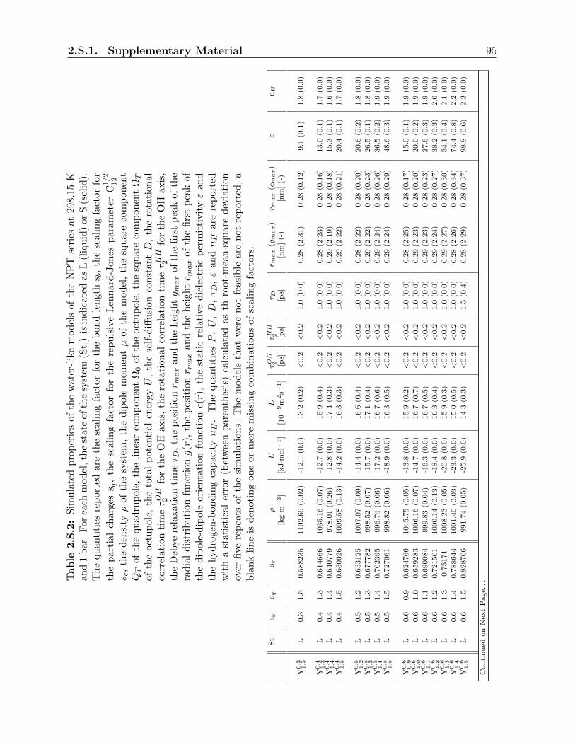
2.S.1. Supplementary Material 95
Table
2.S.2:
Sim
ula
ted
pro
per
ies
ofth
ew
ater
-lik
em
odel
sof
the
NP
Tse
ries
at298.1
5K
and
1b
ar.
For
each
mod
el,th
est
ate
ofth
esy
stem
(St.
)is
ind
icat
edas
L(l
iqu
id)
orS
(soli
d).
Th
equ
anti
ties
rep
orte
dar
eth
esc
alin
gfa
ctor
for
the
bon
dle
ngt
hs b
,th
esc
alin
gfa
ctor
for
the
par
tial
char
ges
s q,
the
scal
ing
fact
orfo
rth
ere
pu
lsiv
eL
enn
ard
-Jon
esp
aram
eter
C1/2
12
s c,
the
den
sityρ
ofth
esy
stem
,th
ed
ipol
em
omen
tµ
ofth
em
od
el,
the
squ
are
com
ponen
tQT
ofth
equ
adru
pol
e,th
eli
nea
rco
mp
onen
tΩ
0of
the
oct
up
ole,
the
squ
are
com
pon
ent
ΩT
ofth
eoct
up
ole,
the
tota
lp
oten
tial
ener
gyU
,th
ese
lf-d
iffu
sion
con
stan
tD
,th
ero
tati
on
al
corr
elat
ion
tim
eτOH
2fo
rth
eO
Hax
is,
the
rota
tion
alco
rrel
atio
nti
meτHH
2fo
rth
eO
Haxis
,th
eD
ebye
rela
xat
ion
tim
eτ D
,th
ep
osit
ionr m
ax
and
the
hei
ghtg m
ax
ofth
efi
rst
pea
kof
the
rad
ial
dis
trib
uti
onfu
nct
iong(r
),th
ep
osit
ionr m
ax
and
the
hei
ghtc m
ax
ofth
efi
rst
pea
kof
the
dip
ole-
dip
ole
orie
nta
tion
fun
ctio
nc(r)
,th
est
atic
rela
tive
die
lect
ric
per
mit
tivit
yε
an
dth
ehyd
roge
n-b
ond
ing
capac
itynH
.T
he
qu
anti
tiesP
,U
,D
,τ D
,ε
andnH
are
rep
ort
edw
ith
ast
atis
tica
ler
ror
(bet
wee
np
aren
thes
is)
calc
ula
ted
asth
root
-mea
n-s
qu
are
dev
iati
on
over
five
rep
eats
ofth
esi
mu
lati
ons.
Th
em
od
els
that
wer
en
otfe
asib
lear
en
otre
port
ed,
ab
lan
kli
ne
isd
enot
ing
one
orm
ore
mis
sin
gco
mb
inat
ion
sof
scal
ing
fact
ors.
St.
s bs q
s cρ
UD
τOH
2τHH
2τ D
r max
(gmax)
r max
(cmax)
εnH
[kg·m−3]
[kJ·m
ol−
1]
[10−9m
2s−
1]
[ps]
[ps]
[ps]
[nm
](-
)[n
m]
(-)
Y0.3
1.5
L0.3
1.5
0.5
88235
1102.6
9(0
.02)
-12.1
(0.0
)13.2
(0.2
)<
0.2
<0.2
1.0
(0.0
)0.2
8(2
.31)
0.2
8(0
.12)
9.1
(0.1
)1.8
(0.0
)
Y0.4
1.3
L0.4
1.3
0.6
14666
1035.1
6(0
.07)
-12.7
(0.0
)15.9
(0.4
)<
0.2
<0.2
1.0
(0.0
)0.2
8(2
.23)
0.2
8(0
.16)
13.0
(0.1
)1.7
(0.0
)
Y0.4
1.4
L0.4
1.4
0.6
40779
978.0
1(0
.26)
-12.8
(0.0
)17.4
(0.3
)<
0.2
<0.2
1.0
(0.0
)0.2
9(2
.19)
0.2
8(0
.18)
15.3
(0.1
)1.6
(0.0
)
Y0.4
1.5
L0.4
1.5
0.6
50026
1009.5
8(0
.13)
-14.2
(0.0
)16.3
(0.3
)<
0.2
<0.2
1.0
(0.0
)0.2
9(2
.22)
0.2
8(0
.21)
20.4
(0.1
)1.7
(0.0
)
Y0.5
1.2
L0.5
1.2
0.6
53125
1007.0
7(0
.09)
-14.4
(0.0
)16.6
(0.4
)<
0.2
<0.2
1.0
(0.0
)0.2
8(2
.22)
0.2
8(0
.20)
20.6
(0.2
)1.8
(0.0
)
Y0.5
1.3
L0.5
1.3
0.6
77782
998.5
2(0
.07)
-15.7
(0.0
)17.1
(0.4
)<
0.2
<0.2
1.0
(0.0
)0.2
9(2
.22)
0.2
8(0
.23)
26.5
(0.1
)1.8
(0.0
)
Y0.5
1.4
L0.5
1.4
0.7
02395
996.7
4(0
.06)
-17.2
(0.0
)16.7
(0.6
)<
0.2
<0.2
1.0
(0.0
)0.2
9(2
.24)
0.2
8(0
.26)
36.5
(0.2
)1.9
(0.0
)
Y0.5
1.5
L0.5
1.5
0.7
27061
998.8
2(0
.06)
-18.9
(0.0
)16.3
(0.5
)<
0.2
<0.2
1.0
(0.0
)0.2
9(2
.24)
0.2
8(0
.29)
48.6
(0.3
)1.9
(0.0
)
Y0.6
0.9
L0.6
0.9
0.6
24766
1045.7
5(0
.05)
-13.8
(0.0
)15.9
(0.2
)<
0.2
<0.2
1.0
(0.0
)0.2
8(2
.25)
0.2
8(0
.17)
15.0
(0.1
)1.9
(0.0
)
Y0.6
1.0
L0.6
1.0
0.6
59283
1006.1
6(0
.07)
-14.7
(0.0
)16.7
(0.7
)<
0.2
<0.2
1.0
(0.0
)0.2
9(2
.23)
0.2
8(0
.20)
20.0
(0.2
)1.9
(0.0
)
Y0.6
1.1
L0.6
1.1
0.6
90084
999.8
3(0
.04)
-16.3
(0.0
)16.7
(0.5
)<
0.2
<0.2
1.0
(0.0
)0.2
9(2
.23)
0.2
8(0
.23)
27.6
(0.3
)1.9
(0.0
)
Y0.6
1.2
L0.6
1.2
0.7
21501
1000.1
4(0
.13)
-18.4
(0.0
)16.3
(0.4
)<
0.2
<0.2
1.0
(0.0
)0.2
9(2
.24)
0.2
8(0
.27)
38.2
(0.3
)2.0
(0.0
)
Y0.6
1.3
L0.6
1.3
0.7
5171
1008.2
3(0
.05)
-20.8
(0.0
)15.9
(0.3
)<
0.2
<0.2
1.0
(0.0
)0.2
9(2
.27)
0.2
8(0
.30)
54.1
(0.4
)2.1
(0.0
)
Y0.6
1.4
L0.6
1.4
0.7
88644
1001.4
0(0
.03)
-23.3
(0.0
)15.0
(0.5
)<
0.2
<0.2
1.0
(0.0
)0.2
8(2
.26)
0.2
8(0
.34)
74.4
(0.8
)2.2
(0.0
)
Y0.6
1.5
L0.6
1.5
0.8
28706
991.7
4(0
.05)
-25.9
(0.0
)14.3
(0.3
)<
0.2
<0.2
1.5
(0.4
)0.2
8(2
.29)
0.2
8(0
.37)
98.8
(0.6
)2.3
(0.0
)
Conti
nu
edon
Nex
tP
age.
..

96 Chapter 2. Tunable
Tab
le2.S
.2–
Conti
nu
ed
St.
s bs q
s cρ
UD
τOH
2τHH
2τ D
r max
(gmax)
r max
(cmax)
εnH
[kg·m−3]
[kJ·m
ol−
1]
[10−9m
2s−
1]
[ps]
[ps]
[ps]
[nm
](-
)[n
m]
(-)
Y0.7
0.8
L0.7
0.8
0.6
50026
997.1
1(0
.11)
-13.8
(0.0
)17.6
(0.6
)<
0.2
<0.2
1.0
(0.0
)0.2
8(2
.21)
0.2
8(0
.17)
15.3
(0.2
)1.9
(0.0
)
Y0.7
0.9
L0.7
0.9
0.6
83901
1002.3
3(0
.07)
-15.8
(0.0
)16.8
(0.2
)<
0.2
<0.2
1.0
(0.0
)0.2
8(2
.23)
0.2
8(0
.21)
22.6
(0.1
)2.0
(0.0
)
Y0.7
1.0
L0.7
1.0
0.7
27061
987.8
2(0
.06)
-17.9
(0.0
)17.0
(0.7
)<
0.2
<0.2
1.0
(0.0
)0.2
9(2
.23)
0.2
8(0
.25)
31.3
(0.2
)2.1
(0.0
)
Y0.7
1.1
L0.7
1.1
0.7
69231
987.4
5(0
.03)
-20.7
(0.0
)16.3
(0.3
)<
0.2
<0.2
1.0
(0.0
)0.2
9(2
.24)
0.2
8(0
.29)
44.3
(0.5
)2.2
(0.0
)
Y0.7
1.2
L0.7
1.2
0.8
07168
1000.7
8(0
.03)
-24.2
(0.0
)15.0
(0.2
)<
0.2
<0.2
1.2
(0.6
)0.2
8(2
.27)
0.2
8(0
.33)
63.3
(0.4
)2.4
(0.0
)
Y0.7
1.3
L0.7
1.3
0.8
50268
1002.4
3(0
.05)
-27.9
(0.0
)13.1
(0.3
)<
0.2
<0.2
1.3
(0.4
)0.2
8(2
.31)
0.2
8(0
.37)
84.7
(1.1
)2.6
(0.0
)
Y0.7
1.4
L0.7
1.4
0.8
99604
994.0
8(0
.05)
-31.9
(0.0
)11.8
(0.3
)<
0.2
0.4
1.8
(0.2
)0.2
8(2
.38)
0.2
8(0
.41)
111.8
(1.3
)2.7
(0.0
)
Y0.7
1.5
L0.7
1.5
0.9
36505
1005.1
1(0
.06)
-37.1
(0.0
)9.0
(0.2
)0.4
0.4
2.4
(0.1
)0.2
8(2
.49)
0.2
8(0
.46)
147.3
(1.8
)2.9
(0.0
)
Y0.8
0.7
L0.8
0.7
0.6
56211
1008.5
2(0
.06)
-14.3
(0.0
)16.6
(0.4
)<
0.2
<0.2
1.0
(0.0
)0.2
9(2
.22)
0.2
8(0
.17)
15.1
(0.2
)2.0
(0.0
)
Y0.8
0.8
L0.8
0.8
0.7
02395
998.2
4(0
.05)
-16.6
(0.0
)16.5
(0.6
)<
0.2
<0.2
1.0
(0.0
)0.2
9(2
.23)
0.2
8(0
.21)
22.2
(0.1
)2.1
(0.0
)
Y0.8
0.9
L0.8
0.9
0.7
45545
1013.0
5(0
.04)
-20.0
(0.0
)15.5
(0.4
)<
0.2
<0.2
1.0
(0.0
)0.2
8(2
.24)
0.2
8(0
.25)
33.8
(0.2
)2.3
(0.0
)
Y0.8
1.0
L0.8
1.0
0.8
00961
1001.0
7(0
.05)
-23.4
(0.0
)15.0
(0.3
)<
0.2
<0.2
1.2
(0.6
)0.2
8(2
.25)
0.2
8(0
.30)
46.9
(0.5
)2.5
(0.0
)
Y0.8
1.1
L0.8
1.1
0.8
56458
995.4
7(0
.02)
-27.6
(0.0
)13.0
(0.1
)<
0.2
<0.2
1.6
(0.5
)0.2
8(2
.30)
0.2
8(0
.35)
62.8
(0.9
)2.7
(0.0
)
Y0.8
1.2
L0.8
1.2
0.9
09091
995.8
5(0
.04)
-32.7
(0.0
)10.4
(0.3
)<
0.2
0.4
1.8
(0.1
)0.2
8(2
.41)
0.2
8(0
.40)
82.4
(1.5
)2.9
(0.0
)
Y0.8
1.3
L0.8
1.3
0.9
55019
1002.8
6(0
.04)
-39.1
(0.0
)7.3
(0.2
)0.6
0.8
3.1
(0.1
)0.2
8(2
.60)
0.2
8(0
.46)
104.2
(1.4
)3.2
(0.0
)
Y0.8
1.4
L0.8
1.4
1.0
0614
998.4
8(0
.08)
-46.2
(0.0
)4.3
(0.1
)1.5
1.7
5.5
(0.2
)0.2
8(2
.88)
0.2
7(0
.53)
121.1
(3.8
)3.4
(0.0
)
Y0.8
1.5
L0.8
1.5
1.0
4745
999.1
6(0
.10)
-55.0
(0.0
)1.7
(0.0
)3.8
3.9
13.6
(0.5
)0.2
8(3
.31)
0.2
7(0
.63)
140.1
(8.8
)3.6
(0.0
)
Y0.9
0.6
L0.9
0.6
0.6
56211
1006.3
7(0
.10)
-14.1
(0.0
)16.6
(0.5
)<
0.2
<0.2
1.0
(0.0
)0.2
9(2
.22)
0.2
8(0
.15)
13.1
(0.2
)2.0
(0.0
)
Y0.9
0.7
L0.9
0.7
0.7
08567
1003.8
1(0
.03)
-16.9
(0.0
)16.1
(0.5
)<
0.2
<0.2
1.0
(0.0
)0.2
9(2
.21)
0.2
8(0
.20)
20.4
(0.2
)2.2
(0.0
)
Y0.9
0.8
L0.9
0.8
0.7
69231
995.8
8(0
.06)
-20.5
(0.0
)15.8
(0.3
)<
0.2
<0.2
1.0
(0.0
)0.2
8(2
.22)
0.2
8(0
.25)
30.4
(0.5
)2.5
(0.0
)
Y0.9
0.9
L0.9
0.9
0.8
28706
999.8
8(0
.03)
-25.2
(0.0
)13.5
(0.3
)<
0.2
<0.2
1.6
(0.7
)0.2
8(2
.26)
0.2
8(0
.30)
44.0
(0.7
)2.7
(0.0
)
Y0.9
1.0
L0.9
1.0
0.8
87233
1004.3
0(0
.05)
-31.2
(0.0
)10.5
(0.3
)<
0.2
0.4
1.7
(0.2
)0.2
8(2
.38)
0.2
8(0
.37)
58.5
(0.5
)3.0
(0.0
)
Y0.9
1.1
L0.9
1.1
0.9
48857
999.3
7(0
.02)
-38.1
(0.0
)6.8
(0.3
)1.2
1.0
2.9
(0.1
)0.2
8(2
.61)
0.2
7(0
.44)
74.5
(0.7
)3.3
(0.0
)
Y1.0
0.6
L1.0
0.6
0.7
02395
1010.7
7(0
.05)
-16.6
(0.0
)16.1
(0.3
)<
0.2
<0.2
1.0
(0.0
)0.2
8(2
.20)
0.2
8(0
.18)
17.3
(0.1
)2.3
(0.0
)
Y1.0
0.7
L1.0
0.7
0.7
70179
1006.5
5(0
.03)
-20.9
(0.0
)14.9
(0.4
)<
0.2
<0.2
1.0
(0.0
)0.2
8(2
.22)
0.2
8(0
.24)
27.0
(0.3
)2.6
(0.0
)
Y1.0
0.8
L1.0
0.8
0.8
44096
998.8
2(0
.04)
-26.3
(0.0
)12.2
(0.3
)<
0.2
<0.2
1.3
(0.4
)0.2
8(2
.28)
0.2
8(0
.30)
38.4
(0.2
)2.9
(0.0
)
Y1.0
0.9
L1.0
0.9
0.9
09091
1005.8
6(0
.03)
-33.9
(0.0
)7.9
(0.0
)0.9
0.8
2.3
(0.2
)0.2
8(2
.50)
0.2
7(0
.38)
53.4
(0.8
)3.2
(0.0
)
Y1.0
1.0
L1.0
1.0
0.9
7352
1002.9
1(0
.04)
-43.4
(0.0
)3.9
(0.1
)1.8
1.9
5.6
(0.3
)0.2
7(2
.93)
0.2
7(0
.48)
66.7
(1.7
)3.5
(0.0
)
Y1.1
0.5
L1.1
0.5
0.6
90084
990.5
2(0
.07)
-15.0
(0.0
)16.7
(0.2
)<
0.2
<0.2
1.0
(0.0
)0.2
9(2
.19)
0.2
8(0
.15)
12.7
(0.1
)2.2
(0.0
)
Y1.1
0.6
L1.1
0.6
0.7
64
998.2
4(0
.03)
-19.8
(0.0
)15.3
(0.2
)<
0.2
<0.2
1.0
(0.0
)0.2
8(2
.19)
0.2
8(0
.21)
21.4
(0.2
)2.6
(0.0
)
Y1.1
0.7
L1.1
0.7
0.8
44096
1000.4
7(0
.05)
-26.3
(0.0
)11.4
(0.3
)<
0.2
<0.2
1.4
(0.2
)0.2
8(2
.28)
0.2
8(0
.29)
32.2
(0.1
)3.0
(0.0
)
Y1.1
0.8
L1.1
0.8
0.9
24214
998.3
3(0
.04)
-35.0
(0.0
)6.5
(0.1
)0.8
1.0
3.0
(0.2
)0.2
8(2
.60)
0.2
7(0
.38)
45.7
(0.5
)3.3
(0.0
)
Y1.1
0.9
L1.1
0.9
0.9
85804
1005.2
5(0
.08)
-47.6
(0.0
)1.9
(0.0
)3.6
3.8
10.4
(0.3
)0.2
7(3
.25)
0.2
7(0
.51)
59.3
(1.0
)3.7
(0.0
)
Y1.2
0.5
L1.2
0.5
0.7
42446
986.2
6(0
.06)
-17.7
(0.0
)15.6
(0.4
)<
0.2
<0.2
1.0
(0.0
)0.2
8(2
.16)
0.2
8(0
.17)
15.4
(0.1
)2.5
(0.0
)
Y1.2
0.6
L1.2
0.6
0.8
28706
1001.7
8(0
.03)
-24.8
(0.0
)11.8
(0.2
)<
0.2
<0.2
1.4
(0.3
)0.2
8(2
.25)
0.2
7(0
.26)
26.0
(0.2
)3.0
(0.0
)
Conti
nu
edon
Nex
tP
age.
..

2.S.1. Supplementary Material 97
Tab
le2.S
.2–
Conti
nu
ed
St.
s bs q
s cρ
UD
τOH
2τHH
2τ D
r max
(gmax)
r max
(cmax)
εnH
[kg·m−3]
[kJ·m
ol−
1]
[10−9m
2s−
1]
[ps]
[ps]
[ps]
[nm
](-
)[n
m]
(-)
Y1.2
0.7
L1.2
0.7
0.9
24214
994.0
2(0
.03)
-34.3
(0.0
)6.1
(0.2
)1.1
1.1
2.9
(0.1
)0.2
8(2
.62)
0.2
7(0
.37)
38.8
(0.5
)3.4
(0.0
)
Y1.2
0.8
L1.2
0.8
1996.4
7(0
.03)
-48.6
(0.0
)1.3
(0.0
)5.1
5.3
15.2
(0.8
)0.2
7(3
.41)
0.2
7(0
.51)
52.7
(1.6
)3.7
(0.0
)
Y1.3
0.4
L1.3
0.4
0.6
90084
1025.8
6(0
.04)
-15.8
(0.0
)15.3
(0.4
)<
0.2
<0.2
1.0
(0.0
)0.2
8(2
.20)
0.2
7(0
.12)
10.8
(0.0
)2.5
(0.0
)
Y1.3
0.5
L1.3
0.5
0.7
96813
999.8
8(0
.04)
-21.9
(0.0
)12.7
(0.3
)<
0.2
<0.2
1.0
(0.3
)0.2
8(2
.19)
0.2
7(0
.21)
19.0
(0.2
)2.9
(0.0
)
Y1.3
0.6
L1.3
0.6
0.8
99604
1003.8
3(0
.03)
-32.1
(0.0
)6.5
(0.1
)0.8
1.1
2.6
(0.2
)0.2
8(2
.54)
0.2
7(0
.33)
31.4
(0.5
)3.4
(0.0
)
Y1.3
0.7
L1.3
0.7
1994.9
4(0
.06)
-46.9
(0.0
)1.4
(0.0
)5.0
5.3
14.5
(0.5
)0.2
7(3
.38)
0.2
7(0
.48)
42.4
(1.1
)3.7
(0.0
)
Y1.4
0.4
L1.4
0.4
0.7
45545
996.2
1(0
.03)
-17.9
(0.0
)14.7
(0.3
)<
0.2
<0.2
1.0
(0.0
)0.2
8(2
.14)
0.2
7(0
.14)
12.4
(0.1
)2.7
(0.0
)
Y1.4
0.5
L1.4
0.5
0.8
62589
1001.6
7(0
.05)
-27.5
(0.0
)8.3
(0.1
)0.7
0.6
1.7
(0.3
)0.2
8(2
.34)
0.2
7(0
.26)
22.6
(0.3
)3.2
(0.0
)
Y1.4
0.6
L1.4
0.6
0.9
85804
993.2
0(0
.04)
-42.0
(0.0
)2.1
(0.0
)3.3
3.3
9.1
(0.2
)0.2
7(3
.12)
0.2
7(0
.41)
35.9
(0.9
)3.7
(0.0
)
Y1.5
0.3
L1.5
0.3
0.6
66667
1042.2
5(0
.07)
-14.6
(0.0
)14.4
(0.3
)<
0.2
<0.2
1.0
(0.0
)0.2
8(2
.18)
0.2
7(0
.07)
7.3
(0.0
)2.5
(0.0
)
Y1.5
0.4
L1.5
0.4
0.8
00961
998.0
9(0
.05)
-21.7
(0.0
)11.4
(0.1
)<
0.2
0.4
1.4
(0.2
)0.2
8(2
.14)
0.2
7(0
.18)
14.3
(0.2
)3.0
(0.0
)
Y1.5
0.5
L1.5
0.5
0.9
36505
1005.3
4(0
.03)
-35.6
(0.0
)3.8
(0.1
)1.7
1.8
4.6
(0.2
)0.2
7(2
.78)
0.2
7(0
.33)
26.4
(0.3
)3.5
(0.0
)


Chapter 3
Solvent-modulated influence of
intramolecular hydrogen-bonding on
the conformational properties of the
hydroxymethyl group in glucose and
galactose: A molecular dynamics
simulation study.
99

100 Chapter 3. Monosaccharides
Abstract
Intramolecular hydrogen-bonding (H-bonding) is commonly regarded as a major determ-
inant of the conformation of (bio)molecules. However, in an aqueous environment, solvent-
exposed H-bonds are likely to represent only a marginal (possibly adverse) conformational
driving as well as steering force. For example, the hydroxymethyl rotamers of glucose (Glc)
and galactose (Gal) permitting the formation of an H-bond with the adjacent hydroxyl
group are not favored in water but, in the opposite, least populated. This is because
in water, solvent-exposed H-bonds are efficiently screened as well as subject to intense
H-bonding competition by the solvent molecules. In the present study, the effect of a
decrease in the solvent polarity on this rotameric equilibrium is probed using molecular
dynamics (MD) simulation. This is done by considering 6 physical solvents (H2O, DMSO,
CH3OH, CHCl3, CCl4 and vacuum) along with 19 artificial water-like solvent models,
where the dielectric permittivity and H-bonding capacity can be varied independently via
a scaling of the oxygen-hydrogen distance and of the atomic partial charges. In the high
polarity solvents, the intramolecular H-bond is observed, but arises as an opportunistic
consequence of the proximity of the H-bonding partners in a given rotameric state. Only
when the polarity of the solvent is decreased does the intramolecular H-bond start to
induce a significant conformational pressure on the rotameric equilibrium. The artificial
solvent series also reveals that the effects of the solvent permittivity and of its H-bonding
capacity mutually enhance each other, with a slightly larger influence of the permittivity.
The hydroxymethyl conformation in hexopyranoses also appears to be particularly sens-
itive to solvent polarity effects, as the H-bond involving the hydroxymethyl group is only
one out of up to five H-bonds forming a network around the ring, each of which is also
affected by the solvent polarity.

3.1. Introduction 101
3.1 Introduction
It is often assumed that intramolecular hydrogen-bonding (H-bonding) exerts a significant
influence on the conformational properties of aqueous (bio)polymers126–128. To discuss this
statement, one should however distinguish132,169–171 between solvent-exposed and buried
H-bonds, and between their respective roles in promoting stability (i.e. as driving forces)
and specificity (i.e. as steering forces; see the Appendix of Ref.132 for a definition of the
concept).
When a specific conformational change is accompanied by the formation of a buried
H-bond, the cost associated with the removal of the H-bonding partners from the solution
environment (desolvation) offsets the electrostatic gain upon formation of the interaction
itself. However, if the desolvation of two potentially H-bonding groups is not accompanied
by H-bond formation upon burial, the corresponding conformation will be penalized by the
desolvation term. Considering the high polarity of water, the desolvation and electrostatic
terms will typically be of comparable magnitudes. As a result, the formation of a buried
H-bond can be thought of as representing a minor (possibly negligible or even, in some
cases, adverse) conformational driving force, but an important conformational steering
force132.
When a specific conformational change is accompanied by the formation of a solvent-
exposed H-bond, the H-bonding partners remain highly solvated, and their interaction is
screened by the solvent dielectric response as well as subject to H-bonding competition
by the solvent molecules. In the case of an aqueous environment, H-bonding interactions
within the solute and between solute and solvent will typically be of comparable mag-
nitudes. As a result, the formation of a solvent-exposed H-bond can be thought of as
representing a minor (possibly negligible or even, in some cases, adverse) conformational
driving as well as steering force132,169–175. According to this interpretation, solvent-exposed
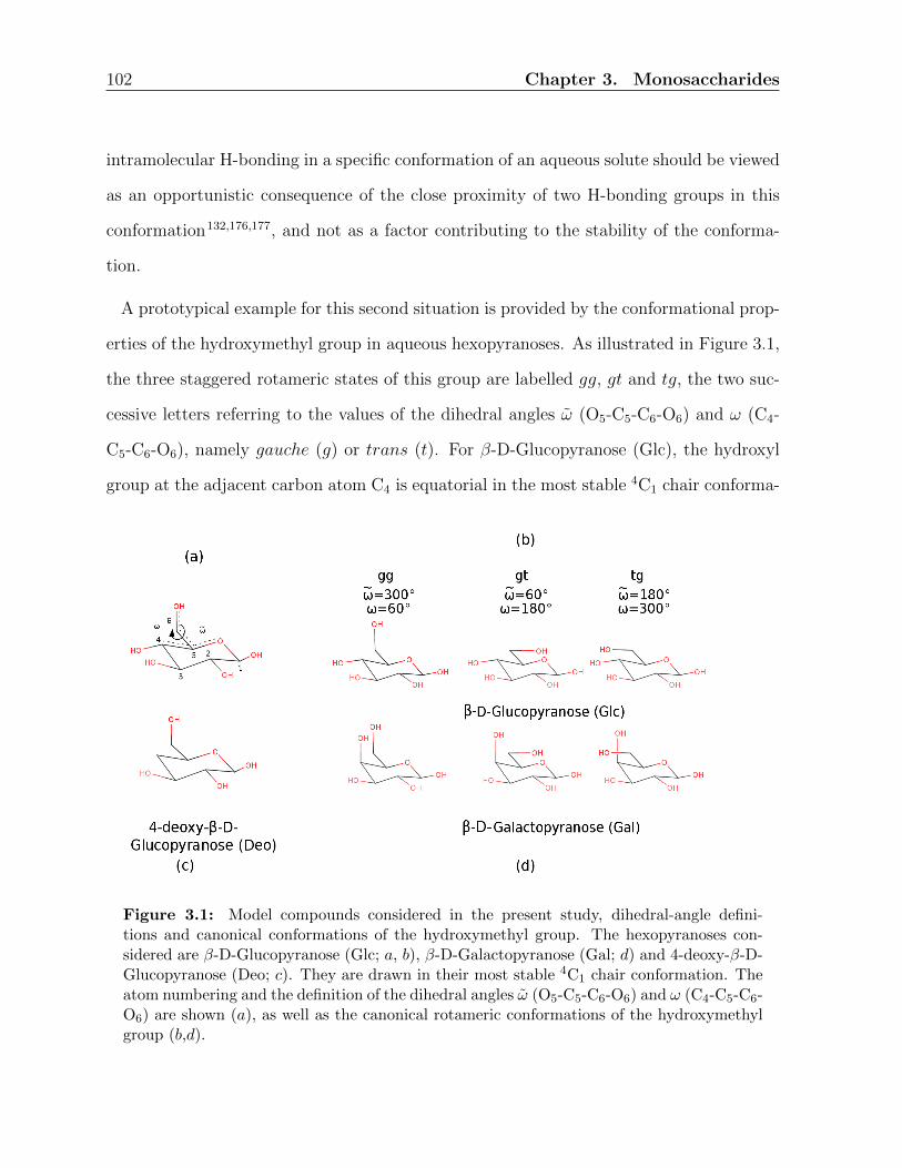
102 Chapter 3. Monosaccharides
intramolecular H-bonding in a specific conformation of an aqueous solute should be viewed
as an opportunistic consequence of the close proximity of two H-bonding groups in this
conformation132,176,177, and not as a factor contributing to the stability of the conforma-
tion.
A prototypical example for this second situation is provided by the conformational prop-
erties of the hydroxymethyl group in aqueous hexopyranoses. As illustrated in Figure 3.1,
the three staggered rotameric states of this group are labelled gg, gt and tg, the two suc-
cessive letters referring to the values of the dihedral angles ω (O5-C5-C6-O6) and ω (C4-
C5-C6-O6), namely gauche (g) or trans (t). For β-D-Glucopyranose (Glc), the hydroxyl
group at the adjacent carbon atom C4 is equatorial in the most stable 4C1 chair conforma-
Figure 3.1: Model compounds considered in the present study, dihedral-angle defini-tions and canonical conformations of the hydroxymethyl group. The hexopyranoses con-sidered are β-D-Glucopyranose (Glc; a, b), β-D-Galactopyranose (Gal; d) and 4-deoxy-β-D-Glucopyranose (Deo; c). They are drawn in their most stable 4C1 chair conformation. Theatom numbering and the definition of the dihedral angles ω (O5-C5-C6-O6) and ω (C4-C5-C6-O6) are shown (a), as well as the canonical rotameric conformations of the hydroxymethylgroup (b,d).

3.1. Introduction 103
tion. As a result, the tg rotamer enables the formation of a solvent-exposed intramolecular
H-bond between these two groups (H4 →O6 or H6 →O4). For β-D-Galactopyranose (Gal),
the hydroxyl group at C4 is axial in the 4C1 chair conformation. As a result, it is the gg
rotamer that enables the formation of this H-bond.
For the two compounds, the rotameric distributions in dilute aqueous solution inferred
from the most recent nuclear magnetic resonance (NMR) experiments184,185,191 are reported
in Table 3.1 (see also Suppl. Mat. Tables 3.S.1 and 3.S.2 for a more extensive compilation
of estimated populations and source J-coupling constants, respectively). They suggest
GlcYear/Ref. gg [%] gt [%] tg [%]
1975178(179) 49 49 21984180 53 45 21988181 53 45 21994182(181) 49 49 22000183 45 62 -72004184 31 61 82006185 31 59 10
GalYear/Ref. gg [%] gt [%] tg [%]
1983186 27 56 171984180(181) 22 53 251987187 22 53 251987188 14 65 211988181 18 62 201994189 12 56 322001190 15 71 142002191 3 67 302004184 3 72 252004184 0 71 29
Table 3.1: Experimentally inferred population estimates for the three staggered rotamersof the hydroxymethyl group of Glc and Gal. The data pertains to aqueous solution and tothe β-anomer of the unmethylated compound. Secondary references between parenthesesindicate that the raw data of the primary reference is quoted as analyzed and reportedin the secondary reference. A more extensive compilation of population estimates alongwith source J-coupling constants (also including α-anomers, O1-methylated derivatives andnon-aqueous solvents) is provided in Suppl. Mat. Tables 3.S.1 and 3.S.2.
104 Chapter 3. Monosaccharides
relative gg:gt:tg populations (in percent) on the order of 30:60:10 for Glc and 5:70:25 for
Gal. In other words, the rotamers permitting the formation of a solvent-exposed H-bond
between the hydroxymethyl group and the hydroxyl group at C4 are not favored but, in
the opposite, least populated.
This observation is compatible with a weak (here, adverse) influence of solvent-exposed
H-bonding on the conformational preferences of the hydroxymethyl group in water. How-
ever, it could also be argued that the experimentally observed preferences actually result
from other stronger effects of steric, stereolectronic or/and electrostatic nature, and thus
do not permit to draw any conclusion on the specific contribution of intramolecular H-
bonding. For example, the stereolectronic gauche-effect182,188,192–206 will favor the gg and
gt conformations for both compounds, and intramolecular H-bonds between the hydroxy-
methyl group and the ring oxygen atom O5 are also in principle possible in these two
conformations. Steric and bond-dipole 1,3-syn repulsions between the C6-O6 and C4-O4
bonds may also be invoked to explain the destabilization of the tg rotamer for Glc and of
the gg rotamer for Gal, if not compensated for by sufficiently strong H-bonding.
Experimentally, different approaches have been employed to tentatively disentangle
the specific role of intramolecular H-bonding from these other effects. The most com-
mon ones involve the consideration of model compounds with altered (non-H-bonding)
substitutions179,182,188–190,200,202,204,207–213 or of non-aqueous solvents with lower polarit-
ies175,179,182,188,200,202,204,207,211,214. Unfortunately, both types of changes do not solely affect
intramolecular H-bonding. For example, the deletion of a hydroxyl group converts a polar
to a non-polar site (aliphatic group), significantly affecting the local solvation properties,
while its replacement by a fluoride atom, although presumably more conservative in terms
of solvation, still affects the steric and stereolectronic properties of the molecule. Simil-
arly, the use of non-aqueous solvents changes not only the dielectric permittivity of the
medium, but simultaneously many other properties of the solvent molecules such as their

3.1. Introduction 105
H-bond donor and acceptor capacities, dispersive interactions, size and shape. As a result,
the contributions of the different effects still remain difficult to disentangle.
Computationally, numerous studies have investigated the problem of the hydroxymethyl
group rotation in hexopyranoses, at the quantum-mechanical190,215–232 (QM) and clas-
sical185,211,233–238 levels. Although they introduce approximations inherent to the physical
model employed, computer-simulation approaches offer three key advantages compared to
experiment: (i) rotameric populations can be monitored directly rather than indirectly,
e.g. by interpretation of experimental NMR J-coupling constants via a specific Karplus re-
lationship191,239–242 and an assumed functional form for the dihedral-angle probability dis-
tribution189,191,204 (e.g. simple three-state population model); (ii) energetic contributions
can be monitored individually, permitting to some extent an analysis of conformational
trends in terms of underlying energy components; (iii) artificial (unphysical) situations
can also be considered.
Because the consideration of unphysical situations in simulations may help disentangling
effects relevant to physical ones, we have recently developed (see Chapter 2) artificial
solvent models derived from the simple point charges (SPC) water model136 by systematic
variation of the oxygen-hydrogen bond length and of the atomic partial charges. These
variations allow for a separate modulation of the dielectric permittivity and H-bonding
capacity of the solvent, while preserving water-like dispersive interactions as well as mo-
lecular size and shape.
In the present work, these artificial solvent models are used to investigate the spe-
cific role of solvent-exposed intramolecular H-bonding on the rotameric properties of
the hydroxymethyl group in Glc and Gal, by monitoring the sensitivity of these prop-
erties to the solvent permittivity and H-bonding capacity. To disentangle the influ-
ence of intramolecular H-bonding from that of the gauche-effect, which is also solvent-

106 Chapter 3. Monosaccharides
dependent170,200,204,206,243, a third compound lacking the hydroxyl group at C4 is also
considered, namely 4-deoxy-β-D-Glucopyranose (Deo), also shown in Figure 3.1. Mo-
lecular dynamics (MD) simulations with the local-elevation umbrella-sampling14 (LEUS)
method to enhance the sampling efficiency along the dihedral angle ω are performed us-
ing the GROMOS 53A6 force field244 and 56A6CARBO force field245,246, considering dif-
ferent physical and artificial solvent models. The physical solvents considered are water
(H2O), dimethyl-sulfoxide (DMSO), methanol (CH3OH), chloroform (CH3Cl) and carbon-
tetrachloride (CCl4), along with vacuum (VAC). The artificial solvents considered are a
subset of 19 among the above-mentioned water-like models with tunable permittivity and
H-bonding capacity (see Chapter 2).
3.2 Computational details
3.2.1 Simulated systems
All MD simulations were carried out using the GROMOS MD++ simulation program81–84
along with two different versions of the GROMOS force field, namely the 53A6 para-
meter set244 and the 56A6CARBO parameter set245. In the context of carbohydrates, the
53A6 parameter set244 is equivalent to the most recent 54A7 set50 and 54A8 set247 of the
GROMOS biomolecular force field, and essentially identical to the 45A4 set developed
for hexopyranose-based carbohydrates by Lins & Hunenberger248 in 2005 (see Ref.245 for
a description of the marginal differences). The 56A6CARBO parameter set of Hansen &
Hunenberger245 results from a complete reoptimization of the 53A6 set in the context of
hexopyranose-based carbohydrates, carried out in 2011. Note that this set was recently
revised246 to a new set 56A6CARBO R, but this change does not affect the compounds
considered here.

3.2. Computational details 107
Sol
vent
ρ[k
g·m−
3]
µ[D
]ε
δHE
xp.
Ref
.Sim
.R
ef.
Exp.
Ref
.Sim
.R
ef.
Exp.
Ref
.Sim
.R
ef.
Exp.
Ref
.H
2O
997
147
973
138
1.85
249
2.27
136
78.5
138
66.0
138
42.3
250
DM
SO
1095
251
1096
149
3.96
166
5.25
149
46.0
251
38.0
149
10.2
250
CH
3O
H79
1251
785
252
1.70
253
2.29
252
32.6
253
19.8
252
22.3
250
CH
Cl 3
1489
251
1520
254
4.81
251
2.30
255
4.8
253
2.4
254
5.7
250
CC
l 415
95253
1601
256
0.00
0.00
2.2
166
1.0
256
-V
AC
--
--
1.0
1.0
-
Table
3.2:
Exp
erim
enta
lan
dsi
mu
late
dp
rop
erti
esof
the
physi
cal
solv
ents
con
sid
ered
inth
ep
rese
nt
stud
yat
298.
15K
and
1b
ar.
Th
equ
anti
ties
rep
orte
dar
eth
ed
ensi
tyρ,
the
gas-
ph
ase
mol
ecu
lar
dip
ole
mom
entµ
,th
est
atic
rela
tive
die
lect
ric
per
mit
tivit
yε,
and
the
Han
sen
par
amet
er250δH
asa
mea
sure
ofth
eH
-bon
din
gp
rop
ensi
ty.

108 Chapter 3. Monosaccharides
The simulations involved computational boxes containing one solute molecule and Ns
solvent molecules. The three solutes considered are β-D-Glucopyranose (Glc), β-D-Galacto-
pyranose (Gal) and 4-deoxy-β-D-Glucopyranose (Deo), see Figure 3.1. The first two com-
pounds differ in the orientation of the hydroxyl group at C4, equatorial for Glc and axial
for Gal in the 4C1 chair conformation, the most stable one in aqueous solution for these
compounds215,245,246,257–263. The last compound lacks the hydroxyl group. In the 53A6
force field, the selection of the hydroxymethyl torsional potentials248 depends on the ori-
entation of the hydroxyl group at C4. For this reason, the definition of a 53A6 topology
for Deo would be ambiguous, and this compound was only simulated with the 56A6CARBO
parameter set. The three solutes were simulated in various physical and artificial solvents.
For the physical solvents, the models considered are the SPC water (H2O) model of
Berendsen et al.136 (Ns = 1200), the dimethyl-sulfoxide (DMSO) model of Geerke et al.149
(Ns = 310), the methanol (CH3OH) model of Walser et al.252 (Ns=1200), the chloroform
(CHCl3) model of Tironi & van Gunsteren254 (Ns = 275), and the carbon-tetrachloride
(CCl4) model of Tironi et al.256 (Ns = 230). The three solutes were also simulated in
vacuum (VAC), using stochastic dynamics100,101 (SD) instead of MD in this specific case.
Basic properties characterising the polarity and H-bonding capacity of the five solvents,
either experimental or based on previous simulations with the indicated models, are sum-
marized in Table 3.2.
The artificial solvents considered are a subset of the tunable solvent models introduced in
Chapter 2 for use under constant-volume (NVT) conditions. These models were generated
starting from the SPC water model136, by changing systematically the oxygen-hydrogen
bond length (scaling factor sb) and the atomic partial charges (scaling factor sq), without
any change in the Lennard-Jones interaction parameters. The scaling factors sb and sq
were both varied systematically by increments of 0.1 in the range 0.1 to 1.5, leading to the
definition of 195 water-like models with different dielectric permittivities and H-bonding

3.2. Computational details 109
Series Solvent sb sq ε nH
SHp
W 0.81.4 0.8 1.4 115 3.4
W 0.91.2 0.9 1.2 89 3.5
W 1.01.0 (SPC) 1.0 1.0 64 3.4W 1.5
0.5 1.5 0.5 25 3.4
Shp
W 0.51.4 0.5 1.4 36 1.7
W 0.80.9 0.8 0.9 33 2.0
W 0.70.6 0.7 0.6 7 1.5
W 0.50.3 0.5 0.3 1 1.4
SPh
W 1.10.9 1.1 0.9 56 3.6
W 1.01.0 (SPC) 1.0 1.0 64 3.4W 0.8
1.1 0.8 1.1 64 2.5W 0.7
1.2 0.7 1.2 65 2.2W 0.6
1.4 0.6 1.4 76 2.0W 0.5
1.5 0.5 1.5 49 1.7
Sph
W 1.50.4 1.5 0.4 14 2.6
W 1.20.5 1.2 0.5 15 2.2
W 1.10.5 1.1 0.5 13 1.9
W 0.80.7 0.8 0.7 15 1.7
W 0.60.9 0.6 0.9 14 1.6
W 0.41.3 0.4 1.3 12 1.5
Table 3.3: Definition and simulated properties of the 19 artificial solvent models consideredin the present study at 298.15 K and 968 kg·m−3. The reported quantities are the scalingfactors sb and sq applied to the oxygen-hydrogen bond length and to the atomic partialcharges, respectively, relative to the SPC water model136, the static relative dielectric per-mittivity ε of the liquid, and the average number nH of H-bonds per molecule in the liquidas a measure of its H-bonding capacity. The models are grouped into four series as describedin section 2.1. Note that the SPC water model W 1.0
1.0 belongs to both series SHp and SPh .These 19 models are a subset of the 195 models developed in Chapter 2, their main ther-modynamic, dynamic, dielectric and H-bonding properties being reported in Suppl. Mat.Table 2.S.1 of Chapter 2.
capacities, but identical dispersive interactions as well as molecular shape and size. Note
that 30 extreme combinations of sb and sq were disregarded, as the corresponding models
could only be simulated with very short timesteps. The 195 artificial models are labelled
Wsbsq according to the values of the two scaling factors, so that in particular W1.0
1.0 is the SPC
water model. The main thermodynamic, dynamical, dielectric and H-bonding properties
of these solvents, as calculated in Chapter 2 based on pure-liquid simulations, are reported
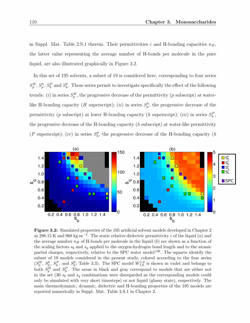
110 Chapter 3. Monosaccharides
in Suppl. Mat. Table 2.S.1 therein. Their permittivities ε and H-bonding capacities nH ,
the latter value representing the average number of H-bonds per molecule in the pure
liquid, are also illustrated graphically in Figure 3.2.
In this set of 195 solvents, a subset of 19 is considered here, corresponding to four series
SHp , Shp , SPh and Sph. These series permit to investigate specifically the effect of the following
trends: (i) in series SHp , the progressive decrease of the permittivity (p subscript) at water-
like H-bonding capacity (H superscript); (ii) in series Shp , the progressive decrease of the
permittivity (p subscript) at lower H-bonding capacity (h superscript); (iii) in series SPh ,
the progressive decrease of the H-bonding capacity (h subscript) at water-like permittivity
(P superscript); (iv) in series Sph, the progressive decrease of the H-bonding capacity (h
Figure 3.2: Simulated properties of the 195 artificial solvent models developed in Chapter 2at 298.15 K and 968 kg·m−3. The static relative dielectric permittivity ε of the liquid (a) andthe average number nH of H-bonds per molecule in the liquid (b) are shown as a function ofthe scaling factors sb and sq applied to the oxygen-hydrogen bond length and to the atomicpartial charges, respectively, relative to the SPC water model136. The squares identify thesubset of 19 models considered in the present study, colored according to the four series(SHp , Shp , SPh , and Sph; Table 3.3). The SPC model W 1.0
1.0 is shown in violet and belongs to
both SHp and SPh . The areas in black and gray correspond to models that are either notin the set (30 sb and sq combinations were disregarded as the corresponding models couldonly be simulated with very short timesteps) or not liquid (glassy state), respectively. Themain thermodynamic, dynamic, dielectric and H-bonding properties of the 195 models arereported numerically in Suppl. Mat. Table 2.S.1 in Chapter 2.

3.2. Computational details 111
subscript) at lower permittivity (p superscript). The main properties of the 19 artificial
solvents considered, along with the definition of the four series, are summarized in Table
3.3 and illustrated graphically in Figure 3.2. Note that the SPC water model W 1.01.0 belongs
to both series SHp and SPh . For the artificial solvents, the number of solvent molecules Ns
in the computational box was always set to 1200.
3.2.2 Simulations
The simulations include explicit-solvent MD simulations of the three solutes (Glc, Gal,
Deo) in the two different sets of solvents (5 physical and 19 artificial) where the sampling
along the dihedral angle ω was enhanced by the LEUS approach14, along with plain SD
simulations100,101 of the three compounds in vacuum.
The MD simulations were performed under periodic boundary conditions based on cubic
computational boxes containing one solute and Ns solvent molecules (values of Ns given in
Section 3.2.1). For the physical solvents, the simulations were carried out in the isothermal-
isobaric (NPT) ensemble at 298.15 K and 1 bar. For the artificial solvents, the simulations
were carried out in the canonical (NVT) ensemble at 298.15 K and an effective solvent
density of 998.3 kg·m−3. Here, the effective solvent density is estimated as V −1M(Ns+Ns),
where V is the box volume, M the molecular mass of water, and Ns an effective number
of water molecules accounting for the solute volume (set here to Ns = 12).
The simulations involving the artificial solvent models must be carried out under NVT
conditions because the Lennard-Jones interaction parameters of these models were not
adjusted to reproduce the equilibrium density of water at 298.15 K and 1 bar. Accord-
ingly, under NVT conditions at 298.15 K and 968 kg·m−3 (as used in Chapter 2), they are
characterized by equilibrium pressures that range from -0.6 to 8.9 kbar for the 19 models
considered here (see Suppl. Mat. Table 2.S.1 in Chapter 2). However, incorrect pressures

112 Chapter 3. Monosaccharides
are expected to have only a limited influence on the rotameric equilibrium of the hydroxy-
methyl group. This was verified explicitly by calculating the relative molar volumes of the
three rotamers at different pressures. Numerical integration of the P∆V terms suggests
relative free energy shifts on the order of 0.4-0.9 kJ·mol−1 for the maximal pressure of 10
kbar. The details of these calculations can be found in Suppl. Mat. Table 3.S.3.
In both the NPT and NVT simulations, the temperature was maintained close to its
reference value of 298.15 K by weakly coupling115 solute and solvent degrees of freedom
jointly (to avoid solute damping264) to an external bath using a relaxation time of 0.1
ps. In the NPT simulations, the pressure was maintained close to its reference value
of 1 bar by weakly coupling115 the atomic coordinates and box dimensions (isotropic
coordinate scaling, group-based virial) to an external bath using a relaxation time of
0.5 ps and an isothermal compressibility of 4.575·10−4 kJ−1·mol·nm3 as appropriate for
aqueous biomolecular systems101. The compressibility was not adjusted for the different
solvents, because it is combined with the arbitrary choice of a pressure relaxation time
and does not affect the average thermodynamic properties of the system. The center of
mass translation of the box was removed every timestep.
The leap-frog algorithm103 was used to integrate Newton’s equations of motion with a
timestep of 2 fs. Solute bond-length constraints as well as the full rigidity of the solvent
molecules were enforced by application of the SHAKE procedure53 with a relative geo-
metric tolerance of 10−4. The non-bonded interactions were calculated using a twin-range
scheme69, with short- and long-range cutoff distances set to 0.8 and 1.4 nm, respectively,
and an update frequency of 5 timesteps for the short-range pairlist and intermediate-range
interactions. A reaction-field correction60,65 was applied to account for the mean effect of
electrostatic interactions beyond the long-range cutoff distance, using the relative dielectric
permittivity appropriate for the solvent model considered (Tables 3.2 and 3.3).
3.2. Computational details 113
The LEUS method14 was applied to improve the conformational sampling around the
dihedral-angle ω (C4-C5-C6-O6, see Figure 3.1) characterizing the orientation of the hy-
droxymethyl group, which can present slow relaxation170,265–269. The LEUS calculations
involved two steps: (i) a local elevation90 (LE) build-up phase of duration tLE = 4 ns,
to progressively optimize a memory-based biasing potential along ω; (ii) an umbrella
sampling105 (US) phase of duration tUS = 40 ns, using this preoptimized (now time-
independent) biasing potential to enhance the sampling. The biasing potential was rep-
resented by means of 36 truncated-polynomial basis functions270 with a spacing of 10.
The polynomial widths were set equal to the grid spacing. The LE build-up phase relied
on a fixed force-constant increment per visit set to kLE = 10−4 kJ·mol−1.
The SD simulations in vacuum were performed by integrating the Langevin equation of
motion100,101. They relied on a reference temperature of 298.15 K and a friction coefficient
of 91 ps−1. The choice of the latter value, appropriate for water100, has no effect on the
average thermodynamic properties of the system. The SD simulations were carried out
for a duration tSD = 1 µs. The LEUS procedure was not applied in this case.
For both the MD+LEUS and the SD simulations, the initial structure of the solute was
in the 4C1 chair conformation. After filling the computational box with molecules of the
solvent considered, the equilibration consisted of a steepest-descent energy minimization,
followed by a 0.5 ps thermalization MD (progressively increased temperature), and by a
1 ns plain MD simulation (constant temperature). From this point, configurations (along
with the value of the biasing potential in the US sampling phases of the LEUS simulations)
were written to file every 0.5 ps for subsequent analysis.

114 Chapter 3. Monosaccharides
3.2.3 Analysis
The analysis of the simulations was performed in terms of: (i) ring conformations; (ii)
probability distribution profiles around ω; (iii) relative populations of the three canonical
hydroxymethyl rotamers; (iv) corresponding relative free energies; (v) occurrence of in-
tramolecular and solute-solvent H-bonds; (vi) correlated probability distributions of the
exocyclic dihedral angles; (vii) calculated NMR J-coupling constants. For the MD+LEUS
simulations, all the thermodynamic and structural quantities analyzed (except the exo-
cyclic dihedral-angle correlations; see below) were calculated based on the configurations
generated during the US sampling phase, with a reweighting factor depending on the value
of the biasing potential associated with each configuration, as detailed elsewhere14.
The ring conformations were assigned based on three out-of-plane dihedral angles α1, α2
and α3 defined according to Pickett & Strauss271 as the values of the improper dihedral
angles C4-O5-C2-C1, O5-C2-C4-C3 and C2-C4-O5-C5, respectively, decreased by 180. The
hexopyranose was considered to be in the 4C1 chair conformation when the three α-angles
were in a range between −17 and −50. For more details about the assignment procedure,
see Ref.14 and Table 2 therein.
The probability distribution profiles p(ω) around ω (C4-C5-C6-O6, see Figure 3.1) were
calculated as normalized histograms using a bin width ∆ω = 2. The canonical conform-
ations of the hydroxymethyl group were defined based on the same dihedral angle. Values
in the ranges [0; 120[, [120; 240[ and [240; 360[ were integrated to define the relat-
ive populations of the gg, tg and gt rotameric states, respectively. Relative free energies
factoring out the influence of the solvent on Deo and on the gt conformer of Glc and Gal
(see Eq. 3.6 below) were also monitored.
For the intramolecular H-bonding analysis, only the H-bonds involving the hydroxy-
methyl group were considered, namely H4 →O6, H6 → O4 and H6 → O5. The occurrence

3.2. Computational details 115
of these three H-bonds was analyzed separately for each rotameric state of the hydroxy-
methyl group. An intramolecular H-bond was assumed to be present when the distance
between the hydrogen and acceptor atoms is below 0.25 nm, and the angle between the
donor, hydrogen and acceptor atoms is above 100. The use of a somewhat relaxed an-
gular criterion170 (a minimum angle of 135 is typically used instead101) is necessary to
encompass H-bonds between the hydroxymethyl group and the ring oxygen atom. The av-
erage numbers of solute-solvent H-bonds involving the hydroxymethyl group, the hydroxyl
group at C4 and the ring oxygen atom O5 were also analyzed, using in this case the normal
angular criterion (minimum angle of 135). For the artificial solvent models involving a
scaling of the oxygen-hydrogen bond length (scaling factor sb 6= 1.0), the solute-solvent
H-bond analysis of each trajectory configuration was preceded by a rescaling of the solvent
oxygen-hydrogen distances as described in Chapter 2. This procedure involves a displace-
ment of the hydrogen atoms of each solvent molecule along the oxygen-hydrogen bond
vector, while keeping the oxygen position fixed, so that the value of 0.1 nm corresponding
to the SPC water model is recovered.
The analysis of correlations between the exocyclic dihedral angles considered the five
dihedral angles ω (C4-C5-C6-O6), φ (O5-C1-O1-H1), χ2 (C1-C2-O2-H2), χ3 (C2-C3-O3-H3)
and χ4 (C3-C4-O4-H4). The dihedral angle χ6 (C5-C6-O6-H6) was omitted from this ana-
lysis, as it is either strongly correlated191 with ω in the presence of an intramolecular
H-bond involving O6, or essentially uncorrelated170,184 in the absence of such an H-bond.
For the above set of five dihedral angles, the correlations were monitored for all possible
pairwise combinations in the form of scatter plots involving successive points sampled at
0.5 ps intervals along the MD+LEUS simulations. No reweighting was applied here, which
corresponds to an artificial situation where the probability distribution p(ω) is essentially
flat. For the discussion, values of χ in the ranges [0, 120[, [120, 240[ and [240, 360[
are labelled g+, t and g−, respectively. This analysis was only performed considering the
116 Chapter 3. Monosaccharides
physical solvents of highest (H2O) and lowest (CCl4) polarities, as well as the two artificial
solvents W 0.50.3 and W 0.4
1.3 presenting the lowest H-bonding capacity (nH = 1.4− 1.5) along
with the lowest or an intermediate permittivity (ε = 1 or 12, respectively).
Finally, for the simulations involving the physical solvents H2O, DMSO and CH3OH, a
direct comparison of the hydroxymethyl rotameric populations with primary experimental
data was performed, namely in terms of the vicinal proton-proton NMR J-coupling con-
stants (3JHH) between the proton at the carbon atom C5 and the R or S protons of the
methylene group C6. The two values, which will be noted JR for 3JH5,H6R and JS for
3JHR,H6S, were calculated based on the simulations considering three alternative Karplus
equations. The Karplus equation of Haasnoot et al. (original version from Ref.241 without
the modification of Ref.272) is given by
3JHH/j0 = 13.86 cos2φ− 0.81 cos φ+I∑i=1
∆χi[0.56− 2.32 cos2(ξiφ+ 17.9|∆χi|)], (3.1)
where j0 = 1 s−1, φ is the dihedral angle between the coupled protons (in degrees, to
be consistent with the value of 17.9 in the last term), I the number of non-hydrogen
substituents Si of the H-C-C-H fragment, ∆χi = χi−χH , χi being the Huggins (unitless)
electronegativity273 of an atom i, and ξi is minus the sign of the H-C-C-Si dihedral angle
in the conformation where the coupled protons are eclipsed. The angle φ corresponds to
ω+δ, with δ = 0 for JR and δ = −120 for JS. For the compounds considered here, I = 3
and Eq. (3.1) is applied with ξi = +1 and -1 for the substituents C4 and O5, respectively,
and with ξi = -1 and +1 for the substituent O6 when evaluating JR and JS, respectively.
The Karplus equation of Tafazzoli & Ghiasi242 is given by
JR/j0 = 5.06 + 0.45 cos(ω)− 0.90 cos(2ω) + 0.80 sin(ω) + 4.65 sin(2ω) (3.2)

3.3. Results 117
and
JS/j0 = 4.86− 1.22 cos(ω) + 4.32 cos(2ω) + 0.04 sin(ω) + 0.07 sin(2ω), (3.3)
where ω is the dihedral angle O5-C5-C6-O6 (see Figure 3.1). Finally, the Karplus equation
of Stenutz et al.191 is given by
JR/j0 = 5.08 + 0.47 cos(ω)− 0.12 cos(2ω) + 0.90 sin(ω) + 4.86 sin(2ω) (3.4)
and
JS/j0 = 4.92− 1.29 cos(ω) + 4.58 cos(2ω) + 0.05 sin(ω) + 0.07 sin(2ω). (3.5)
3.3 Results
3.3.1 Ring conformation
The results concerning the analysis of the ring conformation in the physical solvents are
reported in Table 3.4. Corresponding results for the 19 artificial solvents can be found in
Suppl. Mat. Table 3.S.4. This analysis serves to establish that the leading ring conform-
ation sampled in the simulations is as expected the 4C1 chair conformation. Otherwise,
any subsequent discussion concerning the correlation between the rotameric states and
H-bonding properties of the hydroxymethyl group would be complicated by the presence
of alternative ring conformations, e.g. inverted 1C4 chair, boats or skew-boats. Such con-
formations, which present only marginal populations experimentally for unfunctionalized
hexopyranoses215,245,246,257–263 (with the exception of idose), have been seen to occur in
previous simulations14,170,246,248,274–276 owing to force-field inaccuracies. The 53A6 force

118 Chapter 3. Monosaccharides
field244 is a priori likely to be more prone to ring distortions considering that, unlike the
56A6CARBO force field245 (see also Ref.246 for the revised version CARBO R), its paramet-
erization did not involve the consideration of ring-conformational free energies248.
From the results reported in Tables 3.4 and 3.S.4, it appears that the 4C1 chair con-
formation accounts in all cases for at least 87% of the sampled configurations. The 4C1
populations are tendentially lower for the 56A6CARBO force field compared to the 53A6
force field (contrary to the above expectations) and for Glc compared to Gal, Deo being
53A6 56A6CARBO
Solvent α1 [] α2 [] α3 [] 4C1 Pop. [%] α1 [] α2 [] α3 [] 4C1 Pop. [%]
Glc
H2O -35 (7) -31 (8) -35 (7) 91 -38 (7) -36 (8) -34 (7) 89DMSO -35 (7) -29 (8) -35 (7) 89 -37 (8) -35 (8) -35 (8) 87CH3OH -35 (7) -30 (8) -35 (7) 91 -37 (8) -36 (8) -34 (7) 88CHCL3 -34 (7) -35 (7) -34 (7) 96 -36 (7) -39 (7) -34 (7) 89CCL4 -34 (7) -35 (7) -34 (7) 96 -37 (7) -40 (7) -34 (7) 88VAC -34 (7) -35 (7) -34 (7) 96 -37 (7) -40 (7) -34 (7) 88solvent α1 [] α2 [] α3 [] 4C1 Pop. [%] α1 [] α2 [] α3 [] 4C1 Pop. [%]
Deo
H2O -36 (7) -37 (7) -37 (7) 90DMSO -35 (8) -36 (8) -38 (7) 87CH3OH -36 (7) -36 (8) -37 (7) 89CHCL3 -37 (7) -38 (7) -35 (7) 89CCL4 -37 (7) -38 (7) -35 (7) 90VAC -37 (7) -38 (7) -35 (7) 91solvent α1 [] α2 [] α3 [] 4C1 Pop. [%] α1 [] α2 [] α3 [] 4C1 Pop. [%]
Gal
H2O -31 (7) -38 (6) -36 (6) 94 -36 (7) -38 (7) -36 (7) 92DMSO -30 (7) -38 (6) -36 (6) 93 -35 (7) -39 (7) -36 (7) 90CH3OH -31 (7) -38 (6) -36 (6) 94 -35 (7) -39 (7) -36 (7) 91CHCL3 -33 (6) -36 (6) -35 (6) 97 -38 (7) -37 (7) -33 (7) 92CCL4 -32 (6) -36 (6) -35 (6) 97 -38 (7) -37 (6) -32 (7) 93VAC -34 (7) -35 (7) -34 (7) 96 -37 (7) -40 (7) -34 (7) 88
Table 3.4: Ring-conformational properties of the three compound considered in the phys-ical solvents at 298.15 K and 1 bar. The reported quantities are the Pickett & Stauss dihedralangles271 α1, α2 and α3, and the population of the 4C1 chair conformation (defined by α1,α2 and α3 simultaneously in the range between -17 and -50). The values are calculatedas reweighted averages over the 40 ns US phase of the different LEUS simulations (plainaverage over the 1 µs SD simulations for VAC). The corresponding standard deviations arereported between parentheses. The compounds considered are Glc, Deo and Gal (Figure3.1). The solvents considered are physical solvents of decreasing polarity (Table 3.2). Theforce fields considered are the 53A6 force field244 and the 56A6CARBO force field245. Thesimulations of Deo with 53A6 are omitted due to ambiguous torsional potential definitions.See Suppl. Mat. Table 3.S.4 for corresponding results with the artificial solvents.

3.3. Results 119
intermediate. The values of the Pickett & Strauss dihedral angles271 α1, α2 and α3, aver-
aged over the entire simulation, are in all cases close to the canonical value of −35. The
nature of the solvent has only a limited effect on the 4C1 populations, although DMSO
tends to induce slightly more pronounced ring distortions compared to the other physical
solvents. In all cases, most of the sampled configurations that do not correspond to a 4C1
chair are distorted 4C1 chairs. Only four simulations present brief flips (at most 0.1 ns
duration) to boat conformers, while the 1C4 conformation is never observed.
3.3.2 Hydroxymethyl-group orientation
The normalized probability distributions around the dihedral angle ω defining the orient-
ation of the hydroxymethyl group are displayed in Figure 3.3 for the physical solvents.
Corresponding graphs for the 19 artificial solvents can be found in Suppl. Mat. Figures
3.S.1, 3.S.2 and 3.S.3 (series SHp + Shp , SPh and Sph, respectively). Given the selected LE
build-up and US sampling times tLE = 4 and tUS = 40 ns, respectively, the LEUS simu-
lations provide smooth and well converged probability distributions. The same applies to
the 1 µs SD simulation in vacuum. In all cases, the distributions present relatively narrow
peaks (root-mean-square fluctuations on the order of 10-15) centered close to the three
canonical conformations gg (ω = 60), gt (ω = 180) and tg (ω = 300), with deviations
of the peak position relative to the canonical values on the order of 5 at most (10 for
Gal with the 53A6 force field in some of the artificial solvents). Note that the peak posi-
tions are also slightly shifted when going from the 53A6 to the 56A6CARBO force field, by
about -10, -5 and -10 for gg, gt and tg, respectively. Because the populations can be
unambiguously ascribed to the three canonical rotamers, further discussion of the solvent-
dependent trends is formulated in terms of integrated probability distributions over the
three wells.

120 Chapter 3. Monosaccharides
Figure 3.3: Normalized probability distributions around the dihedral angle ω for the threecompounds considered in the physical solvents at 298.15 K and 1 bar. The values arecalculated as reweighted averages over the 40 ns US phase of the different LEUS simulations(or 1 µs plain SD simulation for VAC) using a bin size of 2. The different panels from left toright correspond to Glc, Deo and Gal (Figure 3.1), and from top to bottom to the series ofphysical solvents (Table 3.2) in order of decreasing polarity. The black curves correspond tothe 53A6 force field244 and the red curves to the 56A6CARBO force field245. The simulationsof Deo with 53A6 are omitted due to ambiguous torsional potential definitions. See Suppl.Mat. Figures 3.S.1-3.S.3 for corresponding results with the artificial solvents.

3.3. Results 121
3.3.3 Relative populations of the rotamers
The populations of the three hydroxymethyl rotamers are displayed in Figure 3.4 for the
physical solvents and in Figures 3.5-3.7 for the artificial solvents (series SHp + Shp , SPh
and Sph, respectively). The data is also reported numerically in Suppl. Mat. Tables 3.S.5
(physical solvents) and 3.S.6-3.S.8 (artificial solvent).
The results obtained using the 53A6 and 56A6CARBO force fields are clearly different.
However, the trends observed along the five series of solvents are qualitatively similar for
the two force fields, the difference arising mainly from an offset in the relative populations
of the three rotamers. Taking water as a reference, the relative gg:gt:tg populations in the
53A6 force field are found to be 56:44:0 for Glc and 34:41:25 for Gal. These results are
consistent with those of previous studies using this force field or the nearly identical 45A4
version (see Suppl. Mat. Table 3.S.1), e.g. 55:45:0 and 34:41:25 in Ref.248 or 57:43:0 and
33:41:26 in Ref.170 (β-anomer, free lactol group). The corresponding relative populations
in the 56A6CARBO force field are found to be 36:59:4 for Glc, 24:56:20 for Deo and 7:53:40
for Gal. For Glc and Gal, this is again consistent with the results of other studies using
this force field (see Suppl. Mat. Table 3.S.1), e.g. 35:60:5 and 6:52:42 in Ref.246 (β-
anomer, free lactol group). The results are also similar to the estimates of 37:60:3 and
7:67:26 in Ref.245 for the corresponding O1-methylated compounds (β-anomer). Note,
however, that if O1-methylation has essentially no influence on the relative populations of
the hydroxymethyl rotamers for Glc, it leads to changes of about 15% in the gt and tg
populations for Gal. This effect was also observed within the 56A6CARBO R force field246
(see Table 7 therein).
The difference between the rotamer populations in the two parameter sets is not entirely
surprising, considering that the 53A6 (45A4) force field248 was calibrated against older
NMR-derived populations181,182,190, whereas the 56A6CARBO force field245 (see also Ref.246)

122 Chapter 3. Monosaccharides
is based on more recent estimates184,185,191, suggesting a slightly lower gg:gt ratio along
with a non-negligible tg population for Glc, and a significantly lower gg population for Gal
(see Table 3.1). Two other differences between the force-field versions should be noted:
(i) 53A6 relies on distinct hydroxymethyl torsional potentials for Glc (equatorial hydroxyl
group at C4 in the 4C1 chair; potential on ω only) and Gal (axial hydroxyl group at
C4 in the 4C1 chair; other potential types on both ω and ω), whereas 56A6CARBO uses
a unique pair of torsional potentials (one on ω and one on ω) for the two compounds;
(ii) 56A6CARBO was validated against primary NMR data in aqueous solution, namely
J-coupling constants, whereas 53A6 was only compared to secondary data, namely NMR-
derived populations. Note, finally, that although the present work considers β-anomers
with a free lactol group, experimental (see Suppl. Mat. Tables 3.S.1 and 3.S.2) and
simulation246 results suggest that α-anomers or/and O1-methylated compounds present
similar J-values and rotamer population ratios in water, with population differences on
the order of 10% or less.
Most of the population discussion below refers to the 56A6CARBO results, considered
to be more accurate. Although the solvent-dependent trends in 53A6 are qualitatively
similar, the main differences are: (i) an underrepresentation of the tg rotamer of Glc, due
to the selection of torsional potentials entirely precluding the occurrence of this rotamer
for aqueous Glc; (ii) an overrepresentation of the gg relative to the gt rotamer of Glc;
(iii) an overrepresentation of the gg relative to the gt and tg rotamers of Gal, the two
latter conformers presenting about the same population ratios in the two force fields.
The following paragraphs summarize the trends observed along five series of solvents,
considering the 56A6CARBO population estimates.
Along the series of physical solvents with decreasing polarity (Figure 3.4; numerical
values in Suppl. Mat. Table 3.S.5), the following trends are observed. For Glc, the
population of tg systematically increases from 4% in H2O to 80% in VAC. The popula-

3.3. Results 123
Figure 3.4: Populations of the three staggered hydroxymethyl rotamers for the threecompounds considered in the physical solvents at 298.15 K and 1 bar. The values arecalculated as reweighted averages over the 40 ns phase of the different LEUS simulations (or1 µs plain SD simulation for VAC). The columns from left to right correspond to Glc, Deo,and Gal (Figure 3.1) using the 53A6 force field244 (middle row) or the 56A6CARBO forcefield245 (bottom row). The bars follow the series of physical solvents (Table 3.2) in order ofdecreasing polarity. The values of the solvent permittivity ε (black circles, scale on the left)and Hansen parameter δH (red triangles, scale on the right) are also displayed (top row).The conformer populations refer to the canonical rotamers gg, gt and tg (Figure 3.1). Thesimulations of Deo with 53A6 are omitted due to ambiguous torsional potential definitions.The data is reported numerically in Suppl. Mat. Table 3.S.5.
tions of gg and gt decrease accordingly, at approximately constant relative ratio. This
is consistent with an increasingly important role of the O4↔O6 intramolecular H-bond,
compatible with the tg rotamer only (Figure 3.1). The sharpest change along the series is
from CH3OH to CHCl3, also associated with the most pronounced decrease in the solvent
polarity. For Gal, the population of gg systematically increases from 7% in H2O to 36%
in VAC, except for CHCl3 with an anomalously high value of 45%. The populations of
gt and tg decrease accordingly, at approximately constant relative ratio except in DMSO
and CH3OH, where the gt:tg ratio is inverted. The general trend is again consistent with

124 Chapter 3. Monosaccharides
an increasingly important role of the O4↔O6 intramolecular H-bond compatible with the
gg rotamer only (Figure 3.1), from destabilizing in H2O to stabilizing in VAC. Finally, for
Deo, one observes an increase of the gt:tg ratio, at approximately constant gg population.
Here also, DMSO and CH3OH represent exceptions, with an inversion of the gt:tg ratio.
As the formation of an O4↔O6 H-bond is impossible in Deo (no hydroxyl group at C4), one
may think that the dominant remaining driving forces are the solvent-dependence of the
gauche-effect and the possible formation of an H6 →O5 H-bond. The former effect would
be expected to increasingly favor the tg rotamer upon decreasing the solvent polarity, as
this conformer has the lowest dipole for the O5-C5-C6-O6 segment. However, the observed
trends are incompatible with this expectation. The formation of a H6 →O5 H-bond would
be expected to increasingly favor the gg and gt conformers, where this H-bond is possible.
The observed trends are not incompatible with this second hypothesis, although only the
gt population increases. Still, it should be stressed that the physical solvent molecules also
vary in shape, size and dispersive interactions, which may affect the rotamer distribution
in a complex and indirect way via specific solvation and packing effects involving the entire
ring.
Along the series SHp of artificial solvents with decreasing permittivity (ε from 115 down
to 25) at water-like H-bonding capacity (nH ≈ 3.4-3.5), see Figure 3.5 (left parts of the
graphs; numerical values in Suppl. Mat. Table 3.S.6), the following trends are observed.
For Glc and Deo, the decreasing permittivity has essentially no influence on the rotameric
equilibrium (except possibly for the last solvent W1.50.5), i.e. the relative rotamer populations
are essentially the same as in water. For Gal, the gg and gt populations slightly increase
at the expense of the tg population (the effect is also more pronounced for the last solvent
W1.50.5).
Along the series Shp of artificial solvents with decreasing permittivity (ε from 36 down
to 1) at low H-bonding capacity (nH ≈ 1.4-2.0), see Figure 3.5 (right parts of the graphs;
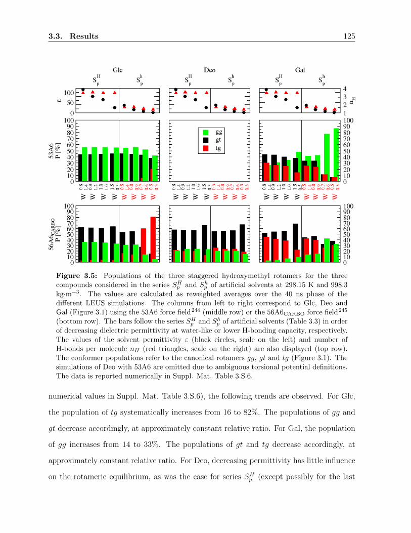
3.3. Results 125
Figure 3.5: Populations of the three staggered hydroxymethyl rotamers for the threecompounds considered in the series SHp and Shp of artificial solvents at 298.15 K and 998.3kg·m−3. The values are calculated as reweighted averages over the 40 ns phase of thedifferent LEUS simulations. The columns from left to right correspond to Glc, Deo andGal (Figure 3.1) using the 53A6 force field244 (middle row) or the 56A6CARBO force field245
(bottom row). The bars follow the series SHp and Shp of artificial solvents (Table 3.3) in orderof decreasing dielectric permittivity at water-like or lower H-bonding capacity, respectively.The values of the solvent permittivity ε (black circles, scale on the left) and number ofH-bonds per molecule nH (red triangles, scale on the right) are also displayed (top row).The conformer populations refer to the canonical rotamers gg, gt and tg (Figure 3.1). Thesimulations of Deo with 53A6 are omitted due to ambiguous torsional potential definitions.The data is reported numerically in Suppl. Mat. Table 3.S.6.
numerical values in Suppl. Mat. Table 3.S.6), the following trends are observed. For Glc,
the population of tg systematically increases from 16 to 82%. The populations of gg and
gt decrease accordingly, at approximately constant relative ratio. For Gal, the population
of gg increases from 14 to 33%. The populations of gt and tg decrease accordingly, at
approximately constant relative ratio. For Deo, decreasing permittivity has little influence
on the rotameric equilibrium, as was the case for series SHp (except possibly for the last

126 Chapter 3. Monosaccharides
solvent W0.50.3).
For Glc and Gal, these trends are qualitatively similar to those observed for the physical
solvents, a decrease in the solvent permittivity favoring the potentially H-bonding con-
former (tg for Glc and gg for Gal). The fact that the corresponding trends are absent (Glc)
or less pronounced (Gal) in series SHp suggests that the effect of the solvent permittivity
only becomes significant when the solvent H-bonding capacity is low. For Deo, the absence
of significant trends along both series SHp and Shp provides a hint that the effects observed
along the physical solvent series are not caused by a change in the solvent permittivity.
Along the series SPh of artificial solvents with decreasing H-bonding capacity (nH from
3.6 down to 1.7) at water-like permittivity (ε ≈ 49− 76), see Figure 3.6 (numerical values
in Suppl. Mat. Table 3.S.7), the following trends are observed. For Glc, the decreasing
H-bonding capacity has a very weak influence on the rotameric equilibrium, with a slight
increase of tg at the expense of gg. For Gal, the influence is also limited, with a small
increase of tg at the expense of gt. For Deo, the population of tg increases slightly, at the
expense of both gg and gt.
Finally, along the series Sph of artificial solvents with decreasing H-bonding capacity (nH
from 2.6 down to 1.5) at low permittivity (ε ≈ 12− 15), see Figure 3.7 (numerical values
in Suppl. Mat. Table 3.S.8), the following trends are observed. For Glc, the population
of tg increases from 11 to 45%. The populations of gg and gt decrease accordingly, at
approximately constant relative ratio. For Gal, the populations of gg and tg increase from
15 to 34% and from 25 to 32%, respectively. The population of gt decreases accordingly.
For Deo, the population of tg increases slightly, at the expense of gg and gt.
For Glc and Gal, the trends along series Sph are similar but more pronounced compared
to those observed along the series SPh , i.e. the effect of a decreasing solvent H-bonding
capacity becomes more significant when the solvent permittivity is low. As was observed
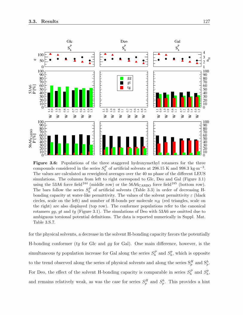
3.3. Results 127
Figure 3.6: Populations of the three staggered hydroxymethyl rotamers for the threecompounds considered in the series SPh of artificial solvents at 298.15 K and 998.3 kg·m−3.The values are calculated as reweighted averages over the 40 ns phase of the different LEUSsimulations. The columns from left to right correspond to Glc, Deo and Gal (Figure 3.1)using the 53A6 force field244 (middle row) or the 56A6CARBO force field245 (bottom row).The bars follow the series SPh of artificial solvents (Table 3.3) in order of decreasing H-bonding capacity at water-like permittivity. The values of the solvent permittivity ε (blackcircles, scale on the left) and number of H-bonds per molecule nH (red triangles, scale onthe right) are also displayed (top row). The conformer populations refer to the canonicalrotamers gg, gt and tg (Figure 3.1). The simulations of Deo with 53A6 are omitted due toambiguous torsional potential definitions. The data is reported numerically in Suppl. Mat.Table 3.S.7.
for the physical solvents, a decrease in the solvent H-bonding capacity favors the potentially
H-bonding conformer (tg for Glc and gg for Gal). One main difference, however, is the
simultaneous tg population increase for Gal along the series SPh and Sph, which is opposite
to the trend observed along the series of physical solvents and along the series SHp and Shp .
For Deo, the effect of the solvent H-bonding capacity is comparable in series SPh and Sph,
and remains relatively weak, as was the case for series SHp and Shp . This provides a hint

128 Chapter 3. Monosaccharides
Figure 3.7: Populations of the three staggered hydroxymethyl rotamers for the threecompounds considered in the series Sph of artificial solvents at 298.15 K and 998.3 kg·m−3.The values are calculated as reweighted averages over the 40 ns phase of the different LEUSsimulations. The columns from left to right correspond to Glc, Deo and Gal (Figure 3.1)using the 53A6 force field244 (middle row) or the 56A6CARBO force field245 (bottom row).The bars follow the series Sph of artificial solvents (Table 3.3) in order of decreasing H-bonding capacity at low permittivity. The values of the solvent permittivity ε (black circles,scale on the left) and number of H-bonds per molecule nH (red triangles, scale on the right)are also displayed (top row). The conformer populations refer to the canonical rotamers gg,gt and tg (Figure 3.1). The simulations of Deo with 53A6 are omitted due to ambiguoustorsional potential definitions. The data is reported numerically in Suppl. Mat. Table 3.S.8.
that the comparatively much larger changes observed along the physical solvent series are
not caused by a change in the solvent H-bonding capacity.
In summary, the study of the four artificial solvent series suggests that, for Glc and Gal,
decreasing solvent permittivity or H-bonding capacity both promote an increase in the
population of the potentially H-bonding conformer (tg for Glc and gg for Gal). However,
these effects appear to be cooperative rather than additive, i.e. the influence of either of
3.3. Results 129
the two parameters only becomes significant when the other parameter is already low. In
contrast, for Deo, the two types of changes have a relatively limited effect and the trends
are not those expected on the basis of the solvent-dependence of the gauche-effect. This
suggests that the more pronounced trends observed for this compound along the physical
solvent series are primary related to other properties of the solvent molecules such as shape
and size, possibly along with the influence of a H6 →O5 H-bond.
3.3.4 Relative free energies of the rotamers
The trends noted in the previous section along the five series of solvents are clearly dom-
inated by the influence of the solvent on the population of the potentially H-bonding
conformer. However, they are somewhat shadowed by the fact that the populations of
the two non-H-bonding conformers also vary, as the populations must add up to 100%.
In addition, population variations for Deo, in which the O4↔O6 H-bond is precluded,
reveal that other influences may be active for the three compounds, such as the solvent-
dependence of the gauche effect, the possible presence of a weak H6 →O5 H-bond and, for
the physical solvent series, the variation of the shape and size of the solvent molecule.
One may attempt to factor out these secondary effects by monitoring for each solvent
the relative free energy
∆∆G(R,C) = [G(R,C)−G(gt,C)]− [G(R,Deo)−G(gt,Deo)]
= −kBT lnp(R,C)p(gt,Deo)
p(gt,C)p(R,Deo),
(3.6)
where R and C denote a rotamer and a compound, respectively, kB is the Boltzmann
constant and T the absolute temperature. These relative free energies, simply noted
∆∆G below, remove as a baseline possible solvent-induced shifts in the free energies of all
conformers of Deo, and of the non-H-bonding conformer gt of Glc and Gal. As a result,

130 Chapter 3. Monosaccharides
∆∆G is only non-zero for the gg and tg conformers of Glc and Gal, and should mainly
characterize the solvent-induced shift in the relative free energies of these two rotameric
states caused by the O4↔O6 H-bond.
The results of this analysis are displayed in Figure 3.8 in terms of ∆∆G values along
the five solvent series. The curves strikingly illustrate that when the above secondary
effects are disregarded, the solvent influences exclusively the relative free energy of the
potentially H-bonding conformer (tg for Glc and gg for Gal), with nearly no effect on that
-8
-6
-4
-2
0
2
4
6
Glc
gttggg
Sp
H S
p
h S
h
P Sh
p
-8
-6
-4
-2
0
2
4
6
Gal
H2O
DM
SO
CH
3OH
CH
Cl 3
CC
l 4
VA
C
-8
-6
-4
-2
0
2
4
6
∆∆G
[k
J m
ol-1
]
-8
-6
-4
-2
0
2
4
6
∆∆G
[kJ
mol
-1]
Figure 3.8: Relative free energies ∆∆G of 3.6 for Glc and Gal in the series of physicalsolvents at 298.15 K and 1 bar, and the four series of artificial solvents at 298.15 K and 998.3kg·m−3. The values are displayed for Glc (top) and Gal (bottom) for the three canonicalrotamers gg, gt and tg (Figure 3.1) along the series of physical solvents (Table 3.2) and thefour series of artificial solvents (Table 3.3), as calculated using the 56A6CARBO force field245.

3.3. Results 131
of the other conformer.
Considering the artificial solvent series, the ∆∆G curves for tg in Glc and gg in Gal
present similar features, see for example the large drop between the second and third
solvents in series Shp and the somewhat higher values for the second and fifth solvents
in series SPh . These irregularities arise because the selected solvents span corresponding
ranges of permittivity ε and H-bonding capacity nH in a somewhat inhomogeneous rather
than smoothly continuous fashion (Table 3.3). The observed variations show that reducing
either of the two parameters ε or nH only has a significant influence on the relative free
energy of the H-bonding rotamer when the other parameter is already low. In series SHp
and SPh , one of the two parameters is decreased while the other remains water-like, and the
∆∆G value for the H-bonding conformer decreases only by about 1-3 kJ mol−1. In series
Shp and Sph, one parameter is decreased while the other is already much lower than the
value appropriate for water, and the ∆∆G value for the H-bonding conformer decreases
much more pronouncedly, by about 2-9 kJ mol−1. The influence of ε (over the considered
range 115 to 1) also appears to be intrinsically larger than that of nH (over the considered
range 3.6 to 1.5), and is more pronounced for Glc compared to Gal.
Along the series of physical solvents, the variations of ∆∆G for the non-H-bonding
conformer are slightly more important, but remain limited (range of about 2 kJ mol−1).
The variations for the H-bonding conformer clearly split the series into two groups, namely
polar (H2O, DMSO and CH3OH) and non-polar (CHCl3, CCl4 and VAC) solvents. The
difference in ∆∆G between the two groups is more pronounced for Glc compared to Gal
(about 13 vs. 7 kJ mol−1, respectively). It is also larger than the corresponding variation
along the artificial solvent series Shp , the one presenting the most pronounced trends (about
9 and 4 kJ mol−1, respectively, for Glc and Gal).

132 Chapter 3. Monosaccharides
3.3.5 Hydrogen-bonding
The occurrence of intramolecular and solute-solvent H-bonds during the simulations was
monitored considering the hydroxyl groups at C4 (except Deo) and C6, as well as the
ring oxygen atom O5. The corresponding numbers of H-bonds in a given instantaneous
configuration were averaged (including reweighting) either over the entire trajectory (av-
erage number N), or separately over subsets of configurations presenting each of the three
hydroxymethyl rotameric states (average numbers Ngg, Ngt and Ntg). Note that N is
not equal to the sum of Ngg, Ngt and Ntg, but to the corresponding population-weighted
sum. The detailed results of this analysis considering the two force fields can be found in
Suppl. Mat., graphically in Figures 3.S.4-3.S.11 and numerically in Tables 3.S.9-3.S.12.
To facilitate the discussion, a subset of these results is presented synoptically in Figure
3.9, restricting the discussion to the 56A6CARBO force field. The results for 53A6 differ
quantitatively, but the trends are qualitatively similar.
The occurrence of intramolecular H-bonds is illustrated in the left column of Figure 3.9.
The first row in each graph shows the conformer populations Pgg, Pgt and Ptg (reported
from Figures 3.4-3.7). The second and third rows show the average numbers Ngg, Ngt,
Ntg and N of O4↔O6 and H6→O5 H-bonds, respectively, where O4↔O6 indicates either
of the flip-flop variants H4→O6 and H6→O4. Since at most one H-bond O4↔O6 and one
H-bond H6→O5 can be formed in a given instantaneous configuration, the values can be
interpreted as fractional occurrences.
As expected based on geometric considerations, the formation of a O4↔O6 H-bond is
nearly exclusively compatible with the tg conformer of Glc and the gg conformer of Gal,
and impossible for Deo. For the two former compounds, the gt conformer expectedly
presents rigorously no occurrence of this H-bond. The same approximately holds for the
third conformer, gg for Glc or tg for Gal, although marginal occurrences can be observed

3.3. Results 133

134 Chapter 3. Monosaccharides
Figure 3.9: [Previous page] Average numbers of intramolecular and solute-solvent H-bondsfor the three compounds considered in the series of physical solvents at 298.15 K and 1 bar,and the four series of artificial solvents at 298.15 K and 998.3 kg·m−3. The values arecalculated as reweighted averages over the 40 ns phase of the different LEUS simulations(plain average over 1µs SD simulations for VAC). All results pertain to the 56A6CARBO
force field245. The panels from top to bottom correspond to Glc, Deo and Gal (Figure3.1). The left and right columns correspond to intramolecular and solute-solvent H-bonds,respectively. In each panel of the left column, the rows from top to the bottom refer to thepopulations P of the three staggered hydroxymethyl rotamers, to the average numbers ofO4↔O6 H-bonds, and to the average numbers of H6→O5 H-bonds. In each panel of the rightcolumn, the rows from top to the bottom refer to the the average numbers of O4↔S, O6↔Sand S→O5 H-bonds, where S is a solvent donor or acceptor site. The average numbers arecalculated over the entire simulation (N) or over the three canonical rotamers separately(Ngg, Ngt, Ntg). A more detailed analysis of the H-bonds is provided in Suppl. Mat. Figures3.S.4-3.S.7 (53A6 force field244) and Figures 3.S.8-3.S.11 (56A6CARBO force field245). Thecorresponding numerical values can be found in Suppl. Mat. Tables 3.S.9-3.S.12.
in some of the solvents with the lowest polarities. In this case, the H-bond has a distorted
geometry that barely fits the cutoff criteria employed in the H-bond assignment.
The occurrence of the O4↔O6 H-bond within the potentially H-bonding conformation
(Ntg for Glc or Ngg for Gal) is generally high and increases along the five solvent series. For
the physical solvent series and the artificial solvent series Shp and Sph, values very close to one
are reached for the least polar solvents, i.e. the intramolecular H-bond is always formed
when the hydroxymethyl rotameric state is compatible with its formation. Simultaneously,
the formation of the H-bond starts to drive the rotameric equilibrium towards this specific
conformer, as visible in the evolution of the populations P , but also in the increase of
the occurrence N of this H-bond over the entire conformational ensemble. In addition,
distorted H-bonds start to present marginal occurrences in the alternative rotamers gg for
Glc and tg for Gal (see above), also indicative of a high conformational pressure towards
intramolecular H-bonding in these solvents. In other words, for the least polar solvents
in these three series, H-bond formation represents a strong driving force directing the
conformational equilibrium of the hydroxymethyl group.
For the artificial solvent series SHp and SPh , the occurrence of the O4↔O6 H-bond within

3.3. Results 135
the potentially H-bonding conformer also increases, but remains below 0.9 even for the
least polar solvent of the series. In addition, the frequent formation of this H-bond does
not promote any shift in the rotameric populations P , and its occurrence N over the entire
conformational ensemble remains below 0.1. In other words, for these two series as well
as for the more polar solvents of the three other series (see above), H-bond formation
represents an opportunistic consequence of the proximity of the H-bonding partners in
a given rotameric state, but not a driving force directing the conformational equilibrium
towards this state.
The O4↔O6 H-bond is a flip-flop H-bond. As can be seen in Suppl. Mat. Figures 3.S.8-
3.S.11, the ratio between the two orientations H4→O6:H6→O4 varies in the approximate
range 90:10 to 10:90 for Glc and Gal, with a tendency to increase upon decreasing the
solvent permittivity.
Based on geometric considerations, the formation of a H6→O5 H-bond is only compatible
with the gg and gt conformers for the three compounds considered and indeed, the tg
conformer presents zero occurrence of this H-bond. This H-bond is also expected to be
intrinsically weaker than the O4↔O6 H-bond, as it involves a five-atom rather than a
six-atom H-bonding ring. It is found with approximately equal occurrences ranging from
0 to about 0.5, depending on the solvent, in the gt conformation of the three compounds
and in the gg conformation of Glc and Deo. Its occurrence is significantly smaller for
the gg conformation of Gal, due to competition with the stronger O4↔O6 H-bond in this
conformation.
The trends concerning the H6→O5 H-bond along the different solvent series are most
visible considering Deo, which does not involve a competing O4↔O6 H-bond. Along the
physical solvent series and the artificial solvent series SHp and Shp , the occurrence of H6→O5
in the gg and gt conformations increases. For the least polar solvents in these series, it
136 Chapter 3. Monosaccharides
represents a driving force promoting an increase in the corresponding populations. This
suggests that the H6→O5 H-bond has a more important conformational influence than
the solvent-dependence of the gauche-effect, which would be expected to stabilize the tg
rotamer upon decreasing the solvent polarity. No significant changes are observed along
the artificial solvent series SPh and Sph, where the occurrences are essentially constant at
about 0.1 and 0.2, respectively, and the population shifts are marginal. When considering
Glc and Gal, the trends in the occurrence of H6→O5 are similar to Deo (except for gg in
Gal, see above), but the contribution of this H-bond to the conformational equilibrium is
masked by the much larger effect of the O4↔O6 H-bond.
The occurrence of solute-solvent H-bonds is illustrated in the right column of Figure
3.9. The three rows in each graph show the average numbers of O4↔S, O6↔S and S→O5
H-bonds, where S denotes a solvent donor or acceptor site, and O4↔S and O6↔S indicate
that two flip-flop variants are possible. Because solute oxygen atoms can form H-bonds
with multiple solvent molecules in a given instantaneous configuration, the values Ngg, Ngt,
Ntg and N should be interpreted here as average numbers of H-bonded solvent molecules.
In most cases, these numbers are highest for O6 (primary hydroxyl group, most exposed
to the solvent), slightly lower for O4 (secondary hydroxyl group, slightly less exposed), and
significantly lower for O5 (least exposed and only an H-bond acceptor), typically ranging
from 0.1 to 2.6 for O6, from 0.1 to 1.9 for O4 and from 0.0 to 0.9 for O5. Expectedly,
the numbers are also lower for the physical solvents DMSO (exclusively H-bond acceptor),
CHCl3 (exclusively and weak H-bond donor), CCl4 (non-H-bonding) and VAC.
Along the artificial solvent series Shp and Sph, the numbers of solute-solvent H-bonds
decrease markedly for the three compounds and the three oxygen atoms considered. For
Glc and Gal, this is in line with the trends observed in the left column of Figure 3.9, i.e. as
solute-solvent H-bonding is reduced, the solute compensates by increasingly populating the
3.3. Results 137
intramolecular O4↔O6 H-bond and the rotamer compatible with this bond. In contrast,
along the artificial solvent series SHp and SPh , the numbers vary much less, with a slight
tendential increase for SHp and decrease for SPh . Here also, for Glc and Gal, this is in
line with the trends observed in the left column of Figure 3.9, i.e. since solute-solvent
H-bonding is preserved, there is less need for intramolecular compensation by the O4↔O6
H-bond.
The competition (or compensation) between intramolecular and solute-solvent H-bonds
is clearly visible when the numbers of solute-solvent H-bonds are resolved in terms of
contributing rotamers. For Deo, solute-solvent H-bonding is essentially the same for the
three rotamers, with the exception of O5 in the tg rotamer. In this rotamer, enhanced
solute-solvent H-bonding is correlated with the impossibility of a weak H6→O5 H-bond.
For Glc and Gal, solute-solvent H-bonding is noticeably weaker for O4 and O6 in the
conformation enabling the O4↔O6 H-bond (tg for Glc and gg for Gal). It is also slightly
higher for O5 in the tg conformation which cannot form a weak H6→O5 H-bond, as was
observed for Deo.
3.3.6 Correlation between the exocyclic groups
The results of the analysis of all pairwise correlations between the exocyclic dihedral angles
ω, φ, χ2, χ3 and χ4 based on the simulations performed using the 56A6CARBO force field
are displayed in Figure 3.10. Corresponding graphs for the 53A6 force field are provided
in Suppl. Mat. Figure 3.S.12. Note that these results involve no reweighting, i.e. they
correspond to an artificial situation where the probability distribution p(ω) is essentially
flat and the hydroxymethyl group samples its three canonical conformations with approx-
imately equal probabilities, irrespective of the compound and solvent. This eliminates the
influence of the solvent on p(ω), discussed in details in the previous sections, permitting to

138 Chapter 3. Monosaccharides
focus on the intramolecular orientational correlations. For this reason, one would expect
the results for the 53A6 and 56A6CARBO parameter sets to be similar. In practice, however,
important differences are observed, because the description of the rotameric preferences
of the lactol group (dihedral angle φ) is not very accurate in 53A6 (see discussions in
Refs.170,245). In the following, only the results for 56A6CARBO are discussed.
The preferential exocyclic-group orientations and intramolecular H-bonding patterns of
hexopyranoses in vacuum have been extensively studied in the past by means of QM cal-
culations190,215,217,218,220–223,225,226,228,277–280, including for Glc215,217,218,221,223,225,226,228,277–279
and Gal228,280. These studies have revealed low-energy conformations involving either
clockwise (CW) or counterclockwise (CC) H-bonded networks217,218,220,221,225,226,228,280, re-
ferring to the orientation of the network as viewed from the β-face of the ring. Most
QM studies suggest that the lowest-energy pattern in vacuum is of the CC type for both
Glc and Gal215,217,218,221,223,225,226,228,277–279. Illustrative structures for H-bonding networks
encountered in the simulations are shown in Figure 3.10 for the three compounds. The
values of the exocyclic dihedral angles corresponding to these structures are also marked
on the correlation plots.
Figure 3.10: [Next page] Pairwise correlations between the exocyclic dihedral angles of Glcand Gal in the physical solvents H2O and CCl4 at 298.15 K and 1 bar, and in the artificialsolvents W 0.4
1.3 and W 0.50.3 at 298.15 K and 998.3 kg·m−3. The individual points correspond
to structures sampled at 0.5 ps intervals along the 40 ns US phase of the different LEUSsimulations using the 56A6CARBO force field245. The successive rows from top to bottomcorrespond to Glc, Deo and Gal (Figure 3.1). The solvents considered (Tables 3.2 and 3.3)are H2O (black), CCl4 (blue), W 0.4
1.3 (red) and W 0.50.3 (orange). The dihedral angles are defined
as C4-C5-C6-O6 (ω), O5-C1-O1-H1 (φ), C1-C2-O2-H2 (χ2), C2-C3-O3-H3 (χ3) and C3-C4-O4-H4 (χ4). On the right, three representative structures (A, B, C) for H-bonding networks(dotted lines) encountered in the simulations are displayed for each of the three compounds.Representative points for these specific structures are also shown on the correlation plots(green triangles).

3.3. Results 139

140 Chapter 3. Monosaccharides
The first structure A involves dihedral angles (φ, χ2, χ3, χ4, ω) in (g−, g+, g−, g+, gg/gt)
for Glc, in (g−, g+, g−, -, gg/gt) for Deo or in (g+, g+, g−, g−, gg/gt) for Gal (the variant
with ω in gt is represented in the figure). This structure is representative of a CC network
involving an O4→O3→O2→O1→O5 H-bond series for Glc and Gal (O3→O2→O1→O5 for
Deo) with an additional H6→O5 H-bond. The second structure B involves dihedral angles
(φ, χ2, χ3, χ4, ω) in (g+, g+, g−, g+, tg) for Glc, in (g+, g+, g−, -, gt) for Deo or in (g−,
g+, g−, g−, gg) for Gal.
This structure is also representative of a CC network. For Glc and Gal, it enables the
formation of an extended O6→O4→O3→O2→O1→O5 H-bond series. For Deo it present
the same H-bonding pattern as A, except that φ is in g+ instead of g−. The third structure
C involves dihedral angles (φ, χ2, χ3, χ4, ω) in (t, t, t, t, tg) for Glc, in (t, t, t, -, gt)
for Deo or in (t, t, g+, t, gg) for Gal. This structure is representative of a CW network.
For Glc, it enables the formation of an O1→O2→O3→O4→O6 H-bond series, for Deo
of an O1→O2→O3 series along with an O6→O5 H-bond, and for Gal of an extended
O1→O2→O3→O4→O6→O5 series.
The results of Figure 3.10 for the solvent CCl4 (blue) clearly evidence a conformational
locking of the (φ, χ2, χ3 ,χ4) dihedral angles within either of the three H-bonding networks
exemplified by the structures A, B or C, similar to what is observed in vacuum based
on the available QM studies. In other words, in CCl4, the correlation patterns in the
dihedral angles can be entirely explained assuming that only these three networks are
significantly populated. For Glc, pattern A involves the hydroxymethyl group in gg or
gt and a H6→O5 H-bond, whereas patterns B and C involve the hydroxymethyl group
in tg and a H6→O4 or a H4→O6 H-bond, respectively. As seen earlier, for this solvent,
the tg rotamer is overwhelmingly populated (80%), and the present analysis shows that
it is not only associated with a very high occurrence of the O4↔O6 H-bond, but also
of the compatible extended H-bonding patterns B and C (each corresponding to one of
3.3. Results 141
the flip-flop variants of this H-bond). Similarly, the gt rotamer, which is also populated
(15%), is not only associated with a high occurrence of the H6→O5 H-bond, but also of the
compatible extended H-bonding pattern A. Analogous considerations apply to Gal, where
pattern A involves again the hydroxymethyl group in gg or gt and a H6→O5 H-bond,
whereas patterns B and C involve the hydroxymethyl group in gg and a H6 →O4 or a
H4 →O6 H-bond, respectively. Here also, the different rotamers are not only associated
with the formation of the indicated H-bond, but of the compatible extended H-bonding
patterns A, B or C. For Deo, the three populated patterns are also A, B and C, but due
to the lack of a hydroxyl group at C4, the (φ, χ2, χ3 ,χ4) dihedral angles are only weakly
correlated with the rotameric state determined by ω.
Considering in particular the correlation between φ and ω, it is seen that the three states
of ω are compatible with any state of φ. In contrast, for Glc and Gal, the trans-state of
φ is essentially precluded in the gt rotamer of both compounds.
In sharp contrast to the case of CCl4, the results of Figure 3.10 for the solvent H2O
(black) evidence a high conformational flexibility of the (φ, χ2, χ3, χ4) dihedral angles,
which can adopt either of their three staggered orientations in a largely uncorrelated
fashion. Still, the areas of the correlation plots presenting a negligible density in CCl4
tend to also present a reduced density in H2O, indicating that the preference for the
networks A, B and C persist, albeit in a highly damped form.
Also shown in Figure 3.10 are results for the artificial solvent presenting the lowest H-
bonding capacity along with the lowest permittivity (W 0.50.3 in series Shp ; ε = 1, nH = 1.4;
orange), or an intermediate permittivity (W 0.41.3 in series Sph; ε = 12, nH = 1.5; red). For
the first solvent, the correlations are very similar to those observed in CCl4. In contrast,
for the second solvent, the correlations are more similar to those observed in H2O. Still,
the areas of the correlation plots presenting a negligible density in CCl4 tend to also

142 Chapter 3. Monosaccharides
present a reduced density in this solvent compared to H2O, i.e. the behavior is in this case
somewhat intermediate between those in the two physical solvents. This suggests again
that the influence of the permittivity on the conformational equilibrium is more important
than that of the H-bonding capacity.
3.3.7 J-coupling constants
In the case of the physical solvents H2O, DMSO and CH3OH, it is possible to compare the
simulation results for the rotameric probability distributions p(ω) to primary experimental
NMR data in the form of scalar coupling constants (J-values). The relevant coupling
constants are the vicinal coupling constants between the proton at carbon atom C5, and
the R or S protons at the methylene group C6, noted JR and JS for simplicity.
An extensive list of experimental JR and JS values reported for Glc or Gal in H2O,
DMSO or CH3OH can be found in Suppl. Mat. Table 3.S.2. The values are provided
for the two compounds in either the α- or the β-anomeric form, and either as a free
hexopyranose or as a O1-methyl-hexopyranoside. For H2O, this corresponds to a set of
42 and 29 independent measurements for Glc and Gal, respectively, covering the year
range 1976-2008. The reported J-values clearly differ between the Glc and the Gal data
subsets. However, the differences between the anomeric forms and functionalizations for
either of the two compounds are not statistically significant compared to the spread in
the values reported by different sources. This suggests that, at least in a highly polar
solvent such as water, the lactol group is too distant from the hydroxymethyl group for
exerting a significant influence on its conformational properties. This suggestion is in line
with the results of independent Glc and Gal simulations246 (see Table 7 therein) showing
a limited influence of O1-anomerization or/and -methylation on the calculated JR and JS
values in water. It is also supported by the analysis of exocyclic dihedral-angle correlations

3.3. Results 143
(previous section) suggesting an absence of significant correlation between φ and ω, except
for the least polar solvents where extended H-bonding networks start to trigger longer-
ranged exocyclic-dihedral correlations. Considering the Glc and the Gal data subsets
without discriminating for anomerization and O1-methylation, it also appears that the
reported JR and JS values do not present a clear convergence trend as a function of the
determination year, which would suggest an accuracy increase over the years due to the
availability of improved NMR spectrometers.
For the above reasons, reference experimental values for JR and JS were averaged sep-
arately for Glc and Gal and for the three solvents over all the corresponding experimental
determinations irrespective of the anomerization and O1-methylation. These averages are
reported in Table 3.5, along with a crude error estimate provided by the corresponding
standard deviations. For DMSO and CH3OH, the data sets are considerably smaller than
for water, with 4 and 3 (DMSO) or 5 and 2 (CH3OH) independent measurements for Glc
and Gal, respectively. The estimated errors are on the order of 0.1-0.3 s−1 for the two
Compound Solvent N. dataExp. Sim.
JR [s−1] JS [s−1] JR [s−1] JS [s−1]
GlcH2O 42 5.8 (0.1) 2.1 (0.1) 6.2 (0.1) 2.7 (0.2)DMSO 4 5.9 (0.1) 1.6 (0.1) 6.7 (0.1) 3.0 (0.2)CH3OH 5 5.5 (0.1) 1.9 (0.1) 6.5 (0.1) 3.4 (0.2)
GalH2O 29 7.8 (0.2) 4.5 (0.3) 6.5 (0.1) 5.3 (0.1)DMSO 3 6.3 (0.1) 6.1 (0.1) 4.5 (0.1) 7.3 (0.1)CH3OH 2 6.4 (0.1) 5.6 (0.1) 5.1 (0.1) 6.4 (0.1)
Table 3.5: Comparison between calculated and experimental J-coupling constants for Glcand Gal in H2O, DMSO and CH3OH at 298.15 K and 1 bar. The J-values JR and JScorrespond to the coupling between the proton H5 at C5 and the protons H6R and H6Sat C6, respectively. The values from the simulations are calculated based on the 40 nsUS phase of the LEUS simulations by application of the Karplus equations of Hasnootat al.241, Tafazzoli and Ghiasi242, or Stenutz et al.191 (Eqs. 3.1-3.5), and the averagedover the three results is reported along with the associated standard deviation. The valuesfrom experiments are based on Suppl. Mat. Table 3.S.2, where the average over the listedmeasurements is reported along with the associated standard deviation. The compoundsconsidered are Glc and Gal (Figure 3.1). The solvents considered are H2O (green), DMSO(blue), and CH3OH (yellow). The force field considered is 56A6CARBO
245. The data isillustrated graphically in Figure 3.11.

144 Chapter 3. Monosaccharides
compounds in the different solvents.
Corresponding estimates from the simulations were obtained based on the p(ω) distribu-
tions using the Karplus equations of Haasnoot et al.241, Tafazzoli & Ghiasi242, or Stenutz
et al.191 (Eqs. 3.1-3.5). The results are also reported in Table 3.5, in the form of averages
over the three Karplus curves, along with the corresponding standard deviation as an error
estimate. The estimated errors are on the order of 0.1-0.2 s−1 for the two compounds in
the different solvents.
The comparison between experimental and simulated J-values is shown in Figure 3.11, in
the form of correlation plots, and of a graph illustrating how the convolution of population
profiles p(ω) with a Karplus equation leads to resulting averaged JR and JS estimates.
For Glc, the effect of the solvent on JR and JS is limited, both experimentally and in
the simulations (variations over a range of about 0.5-1 s−1). This is mainly because the
corresponding p(ω) variation among the three solvents is limited. In the simulations, a
small population shift from gg (low values of JR and JS) to tg (higher values of JR and
Figure 3.11: [Next page] Comparison between calculated and experimental J-couplingconstants for Glc and Gal in H2O, DMSO and CH3OH at 298.15 K and 1 bar. In the left part,correlation between experimental J-coupling constants and values calculated based on the 40ns US phase of the LEUS simulations. The J-values JR and JS correspond to the couplingsbetween the proton H5 at C5 and the protons H6R and H6S at C6, respectively. The valuesfrom the simulations are calculated by application of the Karplus equations of Hasnoot etal.241, Tafazzoli & Ghiasi242, or Stenutz et al.191 (Eqs. 3.1-3.5), and the average over thethree results is reported (point) along with the associated standard deviation (horizontalbar). The values from experiments are from Suppl. Mat. Table 3.S.2, where the average overthe listed measurements is reported (point) along with the associated standard deviation(vertical bar). The compounds considered are Glc and Gal (Figure 3.1). The solventsconsidered are H2O (green), DMSO (blue) and CH3OH (yellow). The force field considered is56A6CARBO
245. The data is reported numerically in Table 3.5. In the right part, comparisonbetween the Karplus curve by Hasnoot et al.241 as a function of the dihedral angle ω andthe normalized probability distributions p(ω) around the dihedral angle ω for Glc and Galin the different solvents based on the simulations using the 56A6CARBO
245 force field. Theranges of the Karplus curve relevant for the calculation of the average J-coupling values aremarked with crosses.

3.3. Results 145
44.
55
5.5
66.
57
7.5
J R e
xp. [
s-1]
5
5.56
6.57
7.58
JR sim. [s-1
]
Glc
, R
11.
52
2.5
33.
54
J S exp
. [s-1
]
1.5
22.5
33.5
44.5
JS sim. [s-1
]
1.5
22.5
33.5
44.5
JS sim. [s-1
]
Glc
, S
5.5
66.
57
7.5
88.
59
J R e
xp. [
s-1]
4
4.55
5.56
6.57
JR sim. [s-1
]
Gal
, R
3.5
44.
55
5.5
66.
57
J S exp
. [s-1
]
4.5
55.5
66.5
77.5
88.5
JS sim. [s-1
]
Gal
, S
11.
52
2.5
33.
54
J S exp
. [s-1
]
1.5
22.5
33.5
44.5
JS sim. [s-1
]
1.5
22.5
33.5
44.5
JS sim. [s-1
]
H2O
DM
SOC
H3O
H
036912
JHH [s-1
]
J R J S
Glc
060
120
180
240
300
36000.
01
0.02
0.03
0.04
0.05
p(ω) [deg-1
]
gggt
tgH
2O
DM
SOC
H3O
H
036912
JHH [s-1
]
Gal
060
120
180
240
300
360
ω [
deg]
00.01
0.02
0.03
0.04
0.05
p(ω) [deg-1
]
gggt
tg

146 Chapter 3. Monosaccharides
JS) between H2O and the two other solvents leads to a slight increase in both calculated
J-values. The trend is not clearly visible in the corresponding experimental values, but
these only vary over a range of about 0.5 s−1. In contrast, for Gal, the effect of the solvent
on JR and JS is larger (variations over a range of about 2 s−1). In the simulations, a
significant population shift from gt (high value of JR, low value of JS) to tg (lower value of
JR, higher value of JS) when changing from H2O to CH3OH and then to DMSO leads to a
systematic decrease of JR and increase of JS along the series. The same trend is observed
experimentally.
Although the simulations capture qualitatively well the experimental trends, the devi-
ations between calculated and experimental J-values remain on the order of 0.5-1.5 s−1,
smaller for Glc than for Gal. This is somewhat larger than the sum of the errors estim-
ated based on the spread in the experimental data and Karplus-equation results. The
discrepancy, which may be at least in part ascribed to force-field inaccuracies, appears in
the form of a constant offset, especially for Gal. This suggests that another main source
of inaccuracy may actually reside in the positions and widths of the peaks in p(ω), rather
than in the corresponding populations. In fact, based on the results for H2O shifting the
positions of each of the three peaks in the calculated p(ω) to the left or to the right (eight
possible combinations) by as little as 5 (or 10) may induce changes of up to 0.5 s−1 (or
1.0 s−1) in JR and JS. Such small displacements are of the same order as the shifts rel-
ative to canonical values typically applied in simple population models used to interprete
the NMR data189,191,204 and the shifts observed between the two force-field versions (see
Section 3.3.3).

3.4. Conclusions 147
3.4 Conclusions
Intra- or intermolecular H-bonding is commonly regarded as a major driving force in
(bio)chemical processes such as conformational changes or host-guest binding. For ex-
ample, considerations involving optimal H-bonding patterns have led to spectacular pre-
dictions concerning the native structures of proteins126 and nucleic acids127 in the 50’s.
However, the view proposed here and in Ref.132 is that in an aqueous environment, the
major conformational influence of H-bonding is limited to buried (as opposed to solvent-
exposed) H-bonds and predominantly represents in this case a steering (as opposed to
driving) force. More specifically, conformations involving mismatches among buried po-
lar groups are strongly penalized, but buried H-bonded groups do not per se contribute
significantly to the stability of a conformation.
In contrast, solvent-exposed H-bonds are considered to represent a minor (possible neg-
ligible or even, in some cases, adverse) conformational driving as well as steering force
in an aqueous environment. They should be viewed as an opportunistic consequence of
the close proximity of two H-bonding groups in a given conformation, and not as a factor
contributing to the stability of this conformation. In the present context, this view is
compatible with the experimental observation that the hydroxymethyl rotamers of Glc
and Gal permitting the formation of a solvent-exposed H-bond between this group and
the hydroxyl group at C4 are not favored but, in the opposite, least populated in water.
The above considerations pertain to an aqueous environment where the solvent-exposed
H-bonded interaction is nearly entirely screened by the solvent dielectric response (high
solvent dielectric permittivity) as well as subject to intense H-bonding competition by the
solvent molecules (high solvent H-bonding capacity). As the polarity of the solvent is de-
creased, solvent-exposed intramolecular H-bonding progressively evolves from a negligible
(here, adverse) to a very significant (favorable) conformational driving force. This evolu-

148 Chapter 3. Monosaccharides
tion is probed here using MD simulations to investigate the rotameric preferences of the
hydroxymethyl group of Glc and Gal as well as Deo, an analogous compound lacking the
hydroxyl group at C4, along physical and artificial solvent series of decreasing polarity. The
artificial series also permit to probe separately the effects of the solvent permittivity and
H-bonding capacity, while factoring out a possible influence of the dispersive interactions,
shape and size of the solvent molecule.
As the solvent polarity is decreased, the populations of the conformers compatible with
the formation of a flip-flop O4↔O6 intramolecular H-bond (tg of Glc and gg of Gal)
indeed increase significantly. Because it lacks a hydroxyl group at C4, Deo evidences
comparatively much less pronounced trends, related in part to the possible formation
of an alternative (weaker) H6→O5 H-bond. Considering the artificial solvent series, the
effects of the solvent permittivity and H-bonding capacity appear to mutually enhance
each other, i.e. the effect of varying one of the two solvent parameters is only significant
when the other parameter is low. Thus, in water, the weak (slightly adverse) role of the
solvent-exposed intramolecular H-bond on the hydroxyl rotameric preferences is due to
both dielectric screening and H-bond competition by the solvent, either of the two being
sufficient alone to suppress the conformational pressure towards the formation of this H-
bond. In lower polarity solvents, however, the influence of the solvent permittivity appears
to be intrinsically stronger than that of the solvent H-bonding capacity.
The analysis of the intramolecular H-bond occurrences and of the exocyclic dihedral-
angle correlations also revealed two additional features.
First, even in high polarity solvents where the solvent-exposed H-bonding does not drive
the hydroxymethyl rotameric equilibrium, the intramolecular H-bond is still found with a
very high occurrence (e.g. about 50% for O4↔O6 in water), a situation described above
as opportunistic H-bond formation. As the solvent polarity is decreased, the occurrence

3.4. Conclusions 149
increases to nearly 100%, This is associated with of a raise of the conformational pressure
towards H-bond formation, i.e. the H-bond starts to drive the rotameric equilibrium.
Expectedly, this change is also correlated with (and, in part, caused by) a decrease of
the number of solute-solvent H-bonds for the interacting partners. The key point here
is that direct (e.g. in MD simulations) or indirect (e.g. experimentally via IR or NMR)
observation of a persistent intramolecular H-bond is a necessary but by no means a suffi-
cient condition for ascribing to this H-bond an important role in determining the preferred
molecular conformation, a conclusion that is often too quickly reached in the literature.
Second, the hydroxymethyl conformation in hexopyranoses is a particularly sensitive
probe for the above solvent effects compared e.g. to simpler organic diols281. The reason
is that for these compounds, the O4↔O6 H-bond (or the weaker O6→O5 H-bond) is only
one out of up to five H-bonds constituting extended clockwise or counterclockwise networks
around the ring, each of which also being affected by the solvent polarity (amplification
effect).
The present study illustrates how MD simulations involving unphysical situations (here,
artificial solvents) can be used to shed more light onto physical ones.

150 Chapter 3. Monosaccharides
3.S.1 Supplementary Material
GlcSvt. Compound Year/Ref. gg [%] gt [%] tg [%]
H2O
α
1984180 56 44 01988181 56 44 01988181 58 56 -141988181 58 46 -41992179 49 49 22000183 47 54 -12004184 40 53 72004184 41 51 8
β
1975178(179) 49 49 21984180 53 45 21988181 53 45 21988181 54 57 -111988181 54 48 -2
1994182(181) 49 49 22000183 45 62 -72004184 31 61 82006185 31 59 10
α-Me
1974282(189) 56 39 51984180 57 38 51988181 58 38 41988181 59 49 -81988181 59 41 0
1988181(189) 58 41 11992202 57 38 51994189 60(54) 51(46) -11(0)1994189 63(54) 52(46) -15(0)1994189 69(55) 55(45) -24(0)1994189 53 47 11994189 57(53) 50(47) -7(0)1998204 48 48 42002190 31 76 -72002190 65 53 -18
β-Me
1984180(181) 50 47 31988181 50 47 31988181 51 58 -91988181 51 49 01992179 55 45 1
1994182(181) 48 50 21994189 50 56 -61995283 20 84 -41995283 7 88 52002284 41 52 72002190 23 85 -82002190 50 62 -13
DM
SO α-Me
1984180 55 45 01984180 53 47 01988181 55 45 01988181 57 57 -141988181 57 47 -41992202 53 47 0
β-Me1992179 51 48 11994182 51 47 2
CH
3O
H
α-Me1994189 56(52) 51(48) -7(0)2002190 27 80 -72002190 62 53 -15
β-Me
2002190 24 81 -52002190 59 56 -151992179 52 48 01994182 51 48 0
Forc
eF
ield
s
CHARMM/CSFF 2002236 66 31 1AMBER/Glycam (α-Me) 2001235 54 40 6OPLS/AA-SEI 2002285 69 27 4GROMOS/Spieser 1999287 48 47 5GROMOS 45A4 2005248 55 45 0GROMOS 45A4 2007170 57 43 0GROMOS 56A6CARBO (β-Me) 2011245 37 60 3GROMOS 56A6CARBO 2015246 35 60 5
GalSvt. Compound Year/Ref. gg [%] gt [%] tg [%]
H2O
α
1983186 25 30 451983186 18 38 441983186 21 36 431987187 21 54 251987187 17 63 201987187 20 60 201988181 22 54 241988181 17 63 201988181 15 62 232004184 3 74 232004184 0 74 26
β
1983186 27 56 171983186 24 66 101983186 27 62 11
1984180(181) 22 53 251987187 22 53 251987187 18 62 201987187 21 59 201987188 14 65 211988181 22 53 251988181 18 62 201988181 16 61 231994189 12 56 322001190 15 71 142002191 3 67 302004184 3 72 252004184 0 71 29
α-Me
1983186 19 57 241983186 14 66 201983186 17 62 211984180 14 47 391987187 21 61 181987187 13 70 171987187 20 67 131988181 21 61 181988181 13 70 171988181 15 69 161992202 14 47 391994182 11 64 252002190 40 69 -92002190 23 63 14
β-Me
1983186 25 52 231983186 21 61 181983186 25 57 18
1984180(181) 22 55 231987187 22 55 231987187 17 65 181987187 21 62 181988181 22 55 231988181 17 65 181988181 15 64 21
1994182(202) 17 58 242002190 45 54 12002190 29 53 18
DM
SO
α-Me1988181 27 30 431988181 20 38 421988181 21 39 40
β-Me1988181 32 27 411988181 27 35 381988181 27 37 36
CH
3O
H α-Me2002190 57 46 -32002190 36 19 45
β-Me2002190 57 47 -42002190 33 28 38
Forc
eF
ield
s
CHARMM/CSFF 2002236 4 75 21AMBER/Glycam (α-Me) 2001235 8 64 28OPLS/AA-SEI 2002285 9 53 38GROMOS/Spieser 1999287 5 70 25GROMOS 45A4 2005248 34 41 25GROMOS 45A4 2007170 33 41 26GROMOS 56A6CARBO (β-Me) 2011245 7 67 26GROMOS 56A6CARBO 2015246 6 52 42
Table 3.S.1: Experimentally inferred population estimates for the three staggered rotamers of the hydroxymethylgroup of Glc and Gal, along with a few calculated values. The anomery (α or β) and possible O1-methylation (α-Meor β-Me) of the compound considered as well as the solvent (H2O, DMSO or CH3OH) are indicated. Selected valuesfrom force-field simulations in water are also listed, referring to the unmethylated β-anomer unless otherwise specified.Values between parentheses represent alternative estimates with positiveness constraints on the populations. Multipleentries for the same literature reference correspond to the use of different raw J-values, Karplus equations or/andpopulation models. Secondary references between parentheses indicate that the raw data of the primary reference isquoted as analyzed and reported in the secondary reference.

3.S.1. Supplementary Material 151
GlcSolvent Compound Year/Ref. JR [s−1] JS [s−1]
H2O
α
1976288 5.8 2.01976289 - 1.91977290 5.8 2.01977291 6.0 1.51983186 5.7 2.81984180 5.8 1.01988181 5.8 1.91995292 5.5 2.32000183 5.40 2.202004184 5.6 2.32007242 5.4 2.32008293 5.40 2.31
β
1976288 5.8 2.01977290 5.8 2.01977291 5.4 1.61983186 5.7 2.81984180 6.0 2.11988181 6.0 2.11995292 6.0 2.32000183 5.95 1.952004184 6.2 2.32007242 6.0 2.32008293 5.95 2.27
α-Me
1976288 5.4 2.21977291 5.4 2.21977290 5.4 2.21983186 5.8 2.81984180 5.4 2.31988181 5.4 2.31992179 5.62 2.241994189 5.49 2.392002190 5.4 2.22008293 5.58 2.32
β-Me
1976288 5.8 2.11977290 5.8 2.11977291 6.1 1.71983186 6.4 2.41988181 6.2 2.31992179 5.89 2.002002191 5.8 2.02002190 5.9 2.02008293 6.14 2.31
DMSOα-Me
1984180 6.1 1.01988181 5.9 1.9
β-Me 1992179 5.56 1.935%H2O/DMSO α-Me 1984180 5.9 1.5
CH3OHα-Me
1992179 5.65 2.371994189 5.64 2.402002190 5.5 2.4
β-Me1992179 5.63 1.812002190 5.25 1.95
Pyridine β-Me 1992179 5.76 2.32
GalSolvent Compound Year/Ref. JR [s−1] JS [s−1]
H2O
α
1983186 6.4 6.41987187 7.9 4.61988181 7.9 4.61995292 7.2 5.22002190 8.3 4.02004184 8.2 4.22007242 8.2 4.2
β
1974282 - 3.81983186 7.8 -1987187 7.8 4.61988181 7.8 4.61995292 7.9 4.42002190 7.6 4.42004184 7.9 4.42007242 7.9 4.4
α-Me
1974282 - 4.61976288 6.4 5.31983186 8.2 4.61984180 7.8 6.01988181 8.3 4.01987187 8.3 4.02002190 8.3 4.0
β-Me
1974282 - 4.41976288 8.5 3.51983186 7.6 4.41987187 8.0 4.41988181 8.0 4.42002190 7.6 4.42002191 8.0 4.3
DMSOα-Me 1988181 6.3 6.2
β-Me1984180 6.3 -1988181 5.9 5.9
5%H2O/DMSO β-Me 1984180 6.6 -
CH3OHα-Me 2002190 6.2 5.7β-Me 2002190 6.6 5.5
Table 3.S.2: Experimentally measured J-coupling constants (3JHH) between the protonsat C5 (H5) and C6 (H6R, H6S) for Glc and Gal. The values indicated as JR and JScorrespond to 3JH5,H6R and 3JH5,H6S, respectively. The anomery (α or β) and possibleO1-methylation (α-Me or β-Me) of the compound considered as well as the solvent (H2O,DMSO, 5% H2O/DMSO, CH3OH or pyridine) are indicated.

152 Chapter 3. Monosaccharides
P ∆Vgt→gg ∆Vgt→tg[bar] [nm3] [nm3]
Glc
1 -0.0014 0.00512·103 0.0001 0.00335·103 -0.0013 0.00037·103 -0.0005 0.000110·103 -0.0010 0.0005
Gal
1 0.0029 0.00262·103 0.0034 0.00255·103 -0.0004 0.00047·103 0.0004 0.000810·103 -0.0006 -0.0004
Table 3.S.3: Partial molar volumes of the gg and tg rotamers of Glc and Gal relative tothe gt rotamer at 298.15 K and at different pressures. The relative volumes ∆Vgt→gg and∆Vgt→tg were calculated based on the box volumes in independent 100 ns NPT simulationsof the compounds in SPC water (1200 molecules) at the indicated pressure, carried outwith the hydroxymethyl group constrained to one of the three rotameric states. Numericalintegration of P∆V from 1 bar to 10 kbar suggests that the pressure increase induces freeenergy shifts ∆Ggt→gg of -0.4 or 0.7 kJ·mol−1 and ∆Ggt→tg of 0.9 or 0.7 kJ·mol−1 for Glcand Gal, respectively.
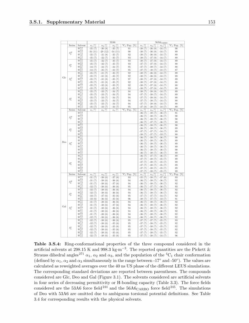
3.S.1. Supplementary Material 153
53A6 56A6CARBO
Series Solvent α1 [] α2 [] α3 [] 4C1 Pop. [%] α1 [] α2 [] α3 [] 4C1 Pop. [%]
Glc
SHp
W 0.81.4 -35 (7) -30 (8) -35 (7) 91 -38 (7) -36 (8) -34 (7) 90
W 0.91.2 -34 (11) -29 (12) -34 (11) 90 -38 (7) -36 (8) -34 (7) 89
W 1.01.0 -35 (7) -31 (8) -35 (7) 92 -38 (7) -36 (8) -34 (7) 89
W 1.50.5 -35 (7) -32 (7) -35 (7) 93 -38 (7) -37 (8) -34 (7) 89
Shp
W 0.51.4 -35 (7) -32 (7) -35 (7) 93 -38 (7) -37 (8) -34 (7) 89
W 0.80.9 -35 (7) -32 (7) -35 (7) 93 -37 (7) -37 (8) -34 (7) 88
W 0.70.6 -34 (7) -34 (7) -34 (7) 95 -37 (7) -39 (7) -34 (7) 88
W 0.50.3 -34 (7) -35 (7) -34 (7) 95 -37 (7) -40 (7) -34 (7) 87
SPh
W 1.10.9 -35 (7) -31 (7) -35 (7) 92 -38 (7) -36 (8) -34 (7) 89
W 1.01.0 -35 (7) -31 (8) -35 (7) 92 -38 (7) -36 (8) -34 (7) 89
W 0.81.1 -35 (7) -31 (8) -35 (7) 97 -38 (7) -37 (8) -34 (7) 89
W 0.71.2 -35 (7) -31 (8) -35 (7) 92 -38 (7) -37 (8) -34 (7) 88
W 0.61.4 -35 (7) -32 (8) -35 (7) 92 -38 (7) -37 (8) -34 (7) 88
W 0.51.5 -35 (7) -32 (8) -35 (7) 93 -38 (7) -37 (8) -34 (7) 89
Sph
W 1.50.4 -35 (7) -33 (7) -34 (7) 94 -38 (7) -38 (8) -34 (7) 89
W 1.20.5 -35 (7) -33 (7) -34 (7) 94 -37 (7) -38 (7) -34 (7) 89
W 1.10.5 -35 (7) -33 (7) -34 (7) 94 -37 (7) -38 (8) -34 (7) 88
W 0.80.7 -35 (7) -33 (7) -34 (7) 94 -37 (7) -38 (7) -34 (7) 88
W 0.60.9 -35 (7) -33 (7) -34 (7) 94 -37 (7) -38 (8) -34 (7) 88
W 0.41.3 -35 (7) -33 (7) -34 (7) 95 -37 (8) -38 (7) -34 (7) 89
Series Solvent α1 [] α2 [] α3 [] 4C1 Pop. [%] α1 [] α2 [] α3 [] 4C1 Pop. [%]
Deo
SHp
W 0.81.4 -36 (7) -38 (7) -36 (7) 91
W 0.91.2 -36 (7) -38 (7) -36 (7) 90
W 1.01.0 -36 (7) -38 (7) -36 (7) 90
W 1.50.5 -36 (7) -37 (7) -36 (7) 89
Shp
W 0.51.4 -36 (7) -38 (7) -36 (7) 90
W 0.80.9 -36 (7) -38 (7) -36 (7) 89
W 0.70.6 -37 (7) -37 (7) -34 (7) 89
W 0.50.3 -38 (7) -37 (7) -33 (7) 88
SPh
W 1.10.9 -36 (7) -38 (7) -36 (7) 90
W 1.01.0 -36 (7) -38 (7) -36 (7) 89
W 0.81.1 -36 (7) -38 (7) -36 (7) 89
W 0.71.2 -36 (7) -38 (7) -36 (7) 89
W 0.61.4 -36 (7) -38 (7) -36 (7) 90
W 0.51.5 -36 (7) -38 (7) -36 (7) 89
Sph
W 1.50.4 -36 (7) -37 (7) -36 (7) 89
W 1.20.5 -37 (7) -38 (7) -35 (7) 89
W 1.10.5 -37 (7) -38 (7) -35 (7) 89
W 0.80.7 -37 (7) -38 (7) -35 (7) 89
W 0.60.9 -37 (7) -38 (7) -35 (7) 89
W 0.41.3 -37 (7) -38 (7) -35 (7) 89
Series Solvent α1 [] α2 [] α3 [] 4C1 Pop. [%] α1 [] α2 [] α3 [] 4C1 Pop. [%]
Gal
SHp
W 0.81.4 -31 (7) -38 (6) -37 (6) 93 -35 (7) -38 (7) -37 (6) 93
W 0.91.2 -31 (7) -38 (6) -36 (6) 94 -36 (7) -38 (7) -36 (7) 92
W 1.01.0 -31 (7) -38 (6) -37 (6) 94 -36 (7) -38 (7) -36 (7) 92
W 1.50.5 -32 (7) -38 (6) -36 (6) 95 -36 (7) -37 (7) -36 (7) 93
Shp
W 0.51.4 -32 (7) -38 (6) -36 (6) 94 -36 (7) -38 (7) -36 (7) 92
W 0.80.9 -32 (7) -38 (6) -36 (6) 94 -36 (7) -38 (7) -36 (7) 92
W 0.70.6 -33 (7) -37 (6) -35 (6) 95 -37 (7) -37 (7) -34 (7) 92
W 0.50.3 -33 (6) -36 (6) -35 (6) 96 -38 (7) -37 (7) -33 (7) 91
SPh
W 1.10.9 -31 (7) -38 (6) -36 (6) 94 -36 (7) -38 (7) -36 (7) 92
W 1.01.0 -31 (7) -38 (6) -37 (6) 94 -36 (7) -38 (7) -36 (7) 92
W 0.81.1 -31 (7) -38 (6) -36 (6) 94 -36 (7) -38 (7) -36 (7) 92
W 0.71.2 -31 (7) -38 (6) -36 (6) 94 -36 (7) -38 (7) -36 (7) 92
W 0.61.4 -31 (7) -38 (6) -36 (6) 94 -36 (7) -38 (7) -36 (7) 92
W 0.51.5 -32 (7) -38 (6) -36 (6) 94 -36 (7) -38 (7) -36 (7) 92
Sph
W 1.50.4 -32 (7) -38 (6) -36 (6) 95 -37 (7) -37 (7) -35 (7) 93
W 1.20.5 -32 (7) -38 (6) -35 (6) 95 -37 (7) -38 (7) -35 (7) 92
W 1.10.5 -32 (7) -38 (6) -35 (6) 95 -37 (7) -38 (7) -35 (7) 92
W 0.80.7 -32 (7) -38 (6) -35 (6) 95 -37 (7) -38 (7) -35 (7) 92
W 0.60.9 -32 (7) -38 (6) -35 (6) 95 -37 (7) -38 (7) -35 (7) 92
W 0.41.3 -32 (7) -38 (6) -35 (6) 95 -37 (7) -38 (7) -34 (7) 96
Table 3.S.4: Ring-conformational properties of the three compound considered in theartificial solvents at 298.15 K and 998.3 kg·m−3. The reported quantities are the Pickett &Strauss dihedral angles271 α1, α2 and α3, and the population of the 4C1 chair conformation(defined by α1, α2 and α3 simultaneously in the range between -17 and -50). The values arecalculated as reweighted averages over the 40 ns US phase of the different LEUS simulations.The corresponding standard deviations are reported between parentheses. The compoundsconsidered are Glc, Deo and Gal (Figure 3.1). The solvents considered are artificial solventsin four series of decreasing permittivity or H-bonding capacity (Table 3.3). The force fieldsconsidered are the 53A6 force field244 and the 56A6CARBO force field245. The simulationsof Deo with 53A6 are omitted due to ambiguous torsional potential definitions. See Table3.4 for corresponding results with the physical solvents.

154 Chapter 3. Monosaccharides
53A6 56A6CARBO
Solvent ε δH gg [%] gt [%] tg [%] gg [%] gt [%] tg [%]
Glc
H2O 61 42.3 56 44 0 36 59 4DMSO 46.7 10.2 47 53 0 26 64 10CH3OH 33 22.3 46 54 0 27 59 14CHCl3 4.8 5.7 40 35 24 6 15 79CCl4 2.2 0 39 45 16 5 15 80VAC 1 0 46 45 9 6 13 80
Deo
H2O 61 42.3 24 56 20DMSO 46.7 10.2 13 35 52CH3OH 33 22.3 17 38 44CHCl3 4.8 5.7 17 66 17CCl4 2.2 0 13 70 17VAC 1 0 15 69 16
Gal
H2O 61 42.3 34 41 25 7 53 40DMSO 46.7 10.2 10 33 56 5 27 68CH3OH 33 22.3 23 36 41 8 35 57CHCl3 4.8 5.7 91 4 5 45 33 21CCl4 2.2 0 86 7 6 27 40 33VAC 1 0 77 16 7 36 36 28
Table 3.S.5: Populations of the three staggered hydroxymethyl rotamers for the threecompounds considered in the physical solvents at 298.15 K and 1 bar. The values arecalculated as reweighted averages over the 40 ns phase of the different LEUS simulations (or1 µs plain SD simulation for VAC). The compounds considered are Glc, Deo and Gal, andthe conformer populations refer to the canonical rotamers gg, gt and tg (Figure 3.1). Thesolvents considered are physical solvents of decreasing polarity (Table 3.2), with indicatedvalues of the permittivity ε and Hansen parameter δH. The force fields considered are the53A6 force field244 and the 56A6CARBO force field245. The simulations of Deo with 53A6 areomitted due to ambiguous torsional potential definitions. The data is illustrated graphicallyin Figure 3.4.
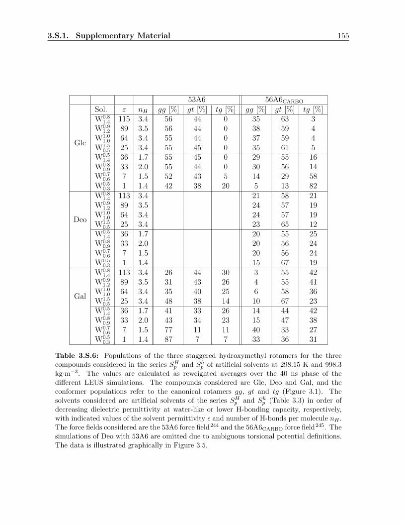
3.S.1. Supplementary Material 155
53A6 56A6CARBO
Sol. ε nH gg [%] gt [%] tg [%] gg [%] gt [%] tg [%]
Glc
W0.81.4 115 3.4 56 44 0 35 63 3
W0.91.2 89 3.5 56 44 0 38 59 4
W1.01.0 64 3.4 55 44 0 37 59 4
W1.50.5 25 3.4 55 45 0 35 61 5
W0.51.4 36 1.7 55 45 0 29 55 16
W0.80.9 33 2.0 55 44 0 30 56 14
W0.70.6 7 1.5 52 43 5 14 29 58
W0.50.3 1 1.4 42 38 20 5 13 82
Deo
W0.81.4 113 3.4 21 58 21
W0.91.2 89 3.5 24 57 19
W1.01.0 64 3.4 24 57 19
W1.50.5 25 3.4 23 65 12
W0.51.4 36 1.7 20 55 25
W0.80.9 33 2.0 20 56 24
W0.70.6 7 1.5 20 56 24
W0.50.3 1 1.4 15 67 19
Gal
W0.81.4 113 3.4 26 44 30 3 55 42
W0.91.2 89 3.5 31 43 26 4 55 41
W1.01.0 64 3.4 35 40 25 6 58 36
W1.50.5 25 3.4 48 38 14 10 67 23
W0.51.4 36 1.7 41 33 26 14 44 42
W0.80.9 33 2.0 43 34 23 15 47 38
W0.70.6 7 1.5 77 11 11 40 33 27
W0.50.3 1 1.4 87 7 7 33 36 31
Table 3.S.6: Populations of the three staggered hydroxymethyl rotamers for the threecompounds considered in the series SHp and Shp of artificial solvents at 298.15 K and 998.3kg·m−3. The values are calculated as reweighted averages over the 40 ns phase of thedifferent LEUS simulations. The compounds considered are Glc, Deo and Gal, and theconformer populations refer to the canonical rotamers gg, gt and tg (Figure 3.1). Thesolvents considered are artificial solvents of the series SHp and Shp (Table 3.3) in order ofdecreasing dielectric permittivity at water-like or lower H-bonding capacity, respectively,with indicated values of the solvent permittivity ε and number of H-bonds per molecule nH .The force fields considered are the 53A6 force field244 and the 56A6CARBO force field245. Thesimulations of Deo with 53A6 are omitted due to ambiguous torsional potential definitions.The data is illustrated graphically in Figure 3.5.

156 Chapter 3. Monosaccharides
53A6 56A6CARBO
Sol. ε nH gg [%] gt [%] tg [%] gg [%] gt [%] tg [%]
Glc
W1.10.9 56 3.6 60 40 0 37 58 5
W1.01.0 64 3.4 55 44 0 37 59 4
W0.81.1 64 2.5 57 43 0 34 60 6
W0.71.2 65 2.2 54 46 0 33 61 6
W0.61.4 76 2.0 52 48 0 32 62 6
W0.51.5 49 1.7 53 47 0 32 58 10
Deo
W1.10.9 56 3.6 24 60 16
W1.01.0 64 3.4 24 57 19
W0.81.1 64 2.5 21 56 23
W0.71.2 65 2.2 21 55 24
W0.61.4 76 2.0 20 56 24
W0.51.5 49 1.7 20 54 26
Gal
W1.10.9 56 3.6 36 40 24 8 56 36
W1.01.0 64 3.4 35 40 25 6 58 36
W0.81.1 64 2.5 32 43 26 7 49 44
W0.71.2 65 2.2 32 41 27 7 50 43
W0.61.4 76 2.0 29 43 28 6 49 45
W0.51.5 49 1.7 33 39 28 10 45 45
Table 3.S.7: Populations of the three staggered hydroxymethyl rotamers for the threecompounds considered in the series SPh of artificial solvents at 298.15 K and 998.3 kg·m−3.The values are calculated as reweighted averages over the 40 ns phase of the different LEUSsimulations. The compounds considered are Glc, Deo and Gal, and the conformer popula-tions refer to the canonical rotamers gg, gt and tg (Figure 3.1). The solvents considered areartificial solvents of the series SPh (Table 3.3) in order of decreasing H-bonding capacity atwater-like permittivity, with indicated values of the solvent permittivity ε and number ofH-bonds per molecule nH . The force fields considered are the 53A6 force field244 and the56A6CARBO force field245. The simulations of Deo with 53A6 are omitted due to ambiguoustorsional potential definitions. The data is illustrated graphically in Figure 3.6.

3.S.1. Supplementary Material 157
53A6 56A6CARBO
Sol. ε nH gg [%] gt [%] tg [%] gg [%] gt [%] tg [%]
Glc
W1.50.4 14 2.6 57 43 0 31 58 11
W1.20.5 15 2.2 56 44 1 28 50 22
W1.10.5 13 1.9 54 44 1 24 44 32
W0.80.7 15 1.7 54 45 1 22 43 35
W0.60.9 14 1.6 54 44 2 21 39 40
W0.41.3 12 1.5 53 45 2 19 36 45
Deo
W1.50.4 14 2.6 23 63 14
W1.20.5 15 2.2 22 59 19
W1.10.5 13 1.9 22 58 20
W0.80.7 15 1.7 21 56 23
W0.60.9 14 1.6 20 55 25
W0.41.3 12 1.5 19 54 27
Gal
W1.50.4 14 2.6 55 30 15 15 60 25
W1.20.5 15 2.2 58 25 16 24 46 30
W1.10.5 13 1.9 64 20 15 29 43 28
W0.80.7 15 1.7 61 21 18 30 39 31
W0.60.9 14 1.6 64 19 17 29 38 33
W0.41.3 12 1.5 65 18 17 34 34 32
Table 3.S.8: Populations of the three staggered hydroxymethyl rotamers for the threecompounds considered in the series Sph of artificial solvents at 298.15 K and 998.3 kg·m−3.The values are calculated as reweighted averages over the 40 ns phase of the different LEUSsimulations. The compounds considered are Glc, Deo and Gal, and the conformer popula-tions refer to the canonical rotamers gg, gt and tg (Figure 3.1). The solvents considered areartificial solvents of the series Sph (Table 3.3) in order of decreasing H-bonding capacity atlow permittivity, with indicated values of the solvent permittivity ε and number of H-bondsper molecule nH . The force fields considered are the 53A6 force field244 and the 56A6CARBO
force field245. The simulations of Deo with 53A6 are omitted due to ambiguous torsionalpotential definitions. The data is illustrated graphically in Figure 3.7.

158 Chapter 3. Monosaccharides
Com
p.
Sol.
53A
656A
6CARBO
H4→
O6
H6→
O4
H6→
O5
H4→
O6
H6→
O4
H6→
O5
tot
gg
gt
tgto
tgg
gt
tgto
tgg
gt
tgto
tgg
gt
tgto
tgg
gt
tgto
tgg
gt
tg
Glc
H2O
0.0
00.0
00.0
00.2
90.0
00.0
00.0
00.2
00.0
20.0
20.0
20.0
00.0
20.0
00.0
00.3
90.0
10.0
00.0
00.2
60.0
80.0
70.0
80.0
0D
MS
O0.0
00.0
00.0
00.3
30.0
00.0
00.0
00.3
60.0
10.0
10.0
10.0
00.0
40.0
00.0
00.4
00.0
50.0
00.0
00.5
00.0
50.0
60.0
50.0
0C
H3O
H0.0
00.0
00.0
00.4
30.0
00.0
00.0
00.3
20.0
30.0
30.0
30.0
00.0
70.0
00.0
00.5
30.0
50.0
00.0
00.3
80.0
80.0
80.0
90.0
0C
HC
l 30.2
30.0
20.0
00.9
20.0
20.0
00.0
00.0
80.1
60.1
90.2
40.0
00.2
50.0
30.0
00.3
10.5
40.0
40.0
00.6
80.0
80.3
40.4
20.0
0C
Cl 4
0.1
30.0
20.0
00.7
90.0
30.0
00.0
00.2
10.2
00.2
40.2
30.0
00.1
00.0
20.0
00.1
20.7
00.0
40.0
00.8
70.0
80.3
60.4
20.0
0V
AC
0.0
90.0
20.0
00.9
90.0
00.0
00.0
00.0
00.2
20.2
40.2
40.0
00.4
00.1
10.0
00.4
90.4
00.0
20.0
00.5
00.0
80.3
10.4
10.0
0
Deo
H2O
--
--
--
--
0.0
60.0
80.0
70.0
0D
MS
O-
--
--
--
-0.0
20.0
50.0
30.0
0C
H3O
H-
--
--
--
-0.0
40.0
80.0
70.0
0C
HC
l 3-
--
--
--
-0.3
40.4
50.4
10.0
0C
Cl 4
--
--
--
--
0.3
40.4
90.3
90.0
0V
AC
--
--
--
--
0.3
40.4
90.3
90.0
0
Gal
H2O
0.0
80.2
30.0
00.0
00.0
40.1
30.0
00.0
00.0
10.0
20.0
20.0
00.0
30.5
20.0
00.0
00.0
10.2
10.0
00.0
00.0
40.0
40.0
80.0
0D
MS
O0.0
40.3
80.0
00.0
00.0
40.4
20.0
00.0
00.0
00.0
00.0
10.0
00.0
20.4
80.0
00.0
00.0
30.5
00.0
00.0
00.0
20.0
10.0
60.0
0C
H3O
H0.1
10.4
90.0
00.0
00.0
60.2
60.0
00.0
00.0
10.0
10.0
20.0
00.0
50.6
50.0
00.0
00.0
30.3
00.0
00.0
00.0
30.0
20.0
90.0
0C
HC
l 30.8
00.8
80.0
00.0
80.0
90.1
00.0
00.0
30.0
70.0
70.1
60.0
00.1
70.3
80.0
00.0
10.2
80.6
10.0
00.0
50.1
70.0
60.4
20.0
0C
Cl 4
0.7
60.8
80.0
00.0
30.0
90.1
00.0
00.0
80.1
20.1
30.1
50.0
00.1
10.4
20.0
00.0
00.1
80.5
70.0
00.0
60.1
80.1
00.3
90.0
0V
AC
0.6
90.8
90.0
00.0
40.0
70.0
80.0
00.0
60.1
30.1
30.1
60.0
00.1
50.4
20.0
10.0
00.2
20.5
60.0
00.0
70.1
80.1
00.3
90.0
1
(a)
Intr
am
ole
cula
rH
-bon
ds
Com
p.
Sol.
53A
656A
6CARBO
O4↔
SO
6↔
SS→
O5
O4↔
SO
6↔
SS→
O5
tot
gg
gt
tgto
tgg
gt
tgto
tgg
gt
tgto
tgg
gt
tgto
tgg
gt
tgto
tgg
gt
tg
Glc
H2O
1.7
01.7
11.6
91.6
92.1
72.1
62.1
92.1
50.6
80.6
70.6
80.7
01.7
41.7
81.7
61.2
82.2
12.1
82.2
71.7
10.4
40.4
50.4
30.4
7D
MS
O0.8
20.8
30.8
20.5
50.9
80.9
80.9
70.6
5-
--
-0.7
10.7
50.7
40.4
40.8
90.9
30.9
30.4
9-
--
-C
H3O
H1.0
91.1
31.0
60.6
81.7
41.7
31.7
51.1
30.3
90.3
80.4
00.3
81.0
51.1
71.1
00.5
61.6
91.7
81.8
01.0
00.1
30.1
40.1
30.1
3C
HC
l 30.0
40.0
40.0
40.0
30.0
80.0
90.1
10.0
20.0
40.0
40.0
30.0
60.0
30.0
60.0
60.0
20.1
10.1
10.1
30.1
00.0
20.0
20.0
10.0
2
Deo
H2O
--
--
2.2
42.2
42.2
62.1
90.5
10.4
80.5
00.5
6D
MS
O-
--
-0.9
50.9
40.9
40.9
6-
--
-C
H3O
H-
--
-1.7
11.7
71.7
21.6
70.1
60.1
50.1
50.1
7C
HC
l 3-
--
-0.1
10.1
20.1
20.0
70.0
20.0
10.0
20.0
3
Gal
H2O
1.7
01.7
11.6
91.6
92.1
72.1
62.1
92.1
50.6
80.6
70.6
80.7
01.7
41.7
81.7
61.2
82.2
12.1
82.2
71.7
10.4
40.4
50.4
30.4
7D
MS
O0.8
20.8
30.8
20.5
50.9
80.9
80.9
70.6
5-
--
-0.7
10.7
50.7
40.4
40.8
90.9
30.9
30.4
9-
--
-C
H3O
H1.0
91.1
31.0
60.6
81.7
41.7
31.7
51.1
30.3
90.3
80.4
00.3
81.0
51.1
71.1
00.5
61.6
91.7
81.8
01.0
00.1
30.1
40.1
30.1
3C
HC
l 30.0
40.0
40.0
40.0
30.0
80.0
90.1
10.0
20.0
40.0
40.0
30.0
60.0
30.0
60.0
60.0
20.1
10.1
10.1
30.1
00.0
20.0
20.0
10.0
2
(b)
Solu
te-s
olv
ent
H-b
ond
s.

3.S.1. Supplementary Material 159
Table 3.S.9: Detailed H-bond analysis for the three compounds in the series of physicalsolvents at 298.15 K and 1 bar. The values are calculated as averages over the 40 ns phaseof the different LEUS simulations (1 µs plain SD simulation for VAC). The compoundsconsidered are Glc, Deo, and Gal (Figure 3.1), along the series of physical solvents (Table3.2) in order of decreasing polarity. The force fields considered are the 53A6 force field244
and the 56A6CARBO force field245. In a, the average numbers of intramolecular H4→O6,H6→O4 and H6→O5 H-bonds are reported. In b, the average numbers of solute-solventO4↔S, O6↔S and S→O5 H-bonds are reported (CCl4 and VAC are omitted as they arenon-H-bonding). The average numbers are calculated either over the entire simulation (N)or over the three canonical rotamers separately, i.e. as Ngg, Ngt and Ntg. The data isillustrated graphically in Suppl. Mat. Figures 3.S.4 and 3.S.8.

160 Chapter 3. Monosaccharides
Table
3.S.10:
Det
aile
dH
-bon
dan
alysi
sfo
rth
eth
ree
com
pou
nd
sin
the
seri
esSH p
andSh p
ofar
tifi
cial
solv
ents
at29
8.15
Kan
d99
8.3
kg·m−
3.
Th
eva
lues
are
calc
ula
ted
asav
erages
over
the
40n
sp
has
eof
the
diff
eren
tL
EU
Ssi
mu
lati
ons.
Th
eco
mp
oun
ds
con
sid
ered
are
Glc
,D
eoan
dG
al(F
igu
re3.
1),
alon
gth
ese
riesSH p
andSh p
ofar
tifi
cial
solv
ents
(Tab
le3.
3)in
ord
erof
dec
reas
ing
die
lect
ric
per
mit
tivit
yat
wat
er-l
ike
orlo
wer
H-b
ond
ing
cap
aci
ty,
resp
ecti
vely
.T
he
forc
efi
eld
sco
nsi
der
edar
eth
e53
A6
forc
efi
eld
244
(lef
t)an
d56
A6 C
AR
BO
forc
efi
eld
245
(rig
ht)
.In
a,th
eav
erag
enu
mb
ers
ofin
tram
olec
ula
rH
4→
O6,
H6→
O4
an
dH
6→
O5
H-b
ond
sar
ere
por
ted
.In
b,
the
aver
age
nu
mb
ers
ofso
lute
-sol
vent
O4↔
S,
O6↔
San
dS→
O5
H-b
ond
sar
ere
por
ted
,w
her
eS
isa
solv
ent
don
oror
acce
pto
rsi
te.
Th
eav
erage
nu
mb
ers
are
calc
ula
ted
eith
erov
erth
een
tire
sim
ula
tion
(N)
orov
erth
eth
ree
can
on
ical
rota
mer
sse
par
atel
y,i.e.
asNgg,Ngt
andNtg
.T
he
dat
ais
illu
stra
ted
grap
hic
ally
inS
up
pl.
Mat
.F
igu
res
3.S
.5an
d3.
S.9
.
(a)
Intr
am
ole
cula
rH
-bon
ds
Com
p.
Sol.
53A
656A
6CARBO
H4→
O6
H6→
O4
H6→
O5
H4→
O6
H6→
O4
H6→
O5
tot
gg
gt
tgto
tgg
gt
tgto
tgg
gt
tgto
tgg
gt
tgto
tgg
gt
tgto
tgg
gt
tg
Glc
W0.8
1.4
0.0
00.0
00.0
00.1
50.0
00.0
00.0
00.0
60.0
10.0
10.0
10.0
00.0
10.0
00.0
00.2
50.0
00.0
00.0
00.1
10.0
30.0
30.0
30.0
0W
0.9
1.2
0.0
00.0
00.0
00.1
20.0
00.0
00.0
00.0
70.0
20.0
20.0
20.0
00.0
10.0
00.0
00.3
70.0
10.0
00.0
00.1
50.0
40.0
40.0
40.0
0W
1.0
1.0
0.0
00.0
00.0
00.2
60.0
00.0
00.0
00.2
00.0
30.0
30.0
30.0
00.0
20.0
00.0
00.4
20.0
10.0
00.0
00.2
40.0
70.0
70.0
80.0
0W
1.5
0.5
0.0
00.0
00.0
00.4
90.0
00.0
00.0
00.2
40.1
00.0
90.1
00.0
00.0
20.0
10.0
00.4
30.0
20.0
00.0
00.3
40.2
20.2
10.2
40.0
0W
0.5
1.4
0.0
00.0
00.0
00.5
60.0
00.0
00.0
00.2
90.0
50.0
50.0
50.0
00.0
90.0
10.0
00.5
30.0
60.0
00.0
00.3
90.1
10.1
30.1
40.0
0W
0.8
0.9
0.0
00.0
00.0
00.5
10.0
00.0
00.0
00.3
20.0
60.0
60.0
60.0
00.0
80.0
10.0
00.5
50.0
50.0
00.0
00.3
60.1
30.1
30.1
60.0
0W
0.7
0.6
0.0
50.0
10.0
00.8
60.0
10.0
00.0
00.1
30.1
60.1
50.1
90.0
00.2
50.0
20.0
00.4
30.3
30.0
20.0
00.5
60.1
40.2
70.3
50.0
0W
0.5
0.3
0.1
90.0
20.0
00.8
70.0
30.0
00.0
00.1
30.1
90.2
20.2
50.0
00.1
80.0
30.0
00.2
20.6
40.0
40.0
00.7
80.0
70.3
50.4
30.0
0
Deo
W0.8
1.4
--
--
--
--
0.0
20.0
30.0
20.0
0W
0.9
1.2
--
--
--
--
0.0
30.0
40.0
40.0
0W
1.0
1.0
--
--
--
--
0.0
60.0
90.0
60.0
0W
1.5
0.5
--
--
--
--
0.1
90.2
40.2
10.0
0W
0.5
1.4
--
--
--
--
0.0
90.1
30.1
10.0
0W
0.8
0.9
--
--
--
--
0.1
00.1
40.1
20.0
0W
0.7
0.6
--
--
--
--
0.2
50.3
50.3
10.0
0W
0.5
0.3
--
--
--
--
0.3
40.4
70.4
00.0
0
Gal
W0.8
1.4
0.0
30.1
10.0
00.0
00.0
10.0
40.0
00.0
00.0
00.0
10.0
10.0
00.0
10.4
40.0
00.0
00.0
00.0
90.0
00.0
00.0
20.0
30.0
30.0
0W
0.9
1.2
0.0
60.1
80.0
00.0
00.0
20.0
60.0
00.0
00.0
10.0
10.0
10.0
00.0
20.4
70.0
00.0
00.0
10.1
60.0
00.0
00.0
30.0
30.0
40.0
0W
1.0
1.0
0.0
90.2
50.0
00.0
00.0
40.1
00.0
00.0
00.0
10.0
20.0
20.0
00.0
30.5
10.0
00.0
00.0
10.2
00.0
00.0
00.0
50.0
40.0
80.0
0W
1.5
0.5
0.1
40.2
90.0
00.0
00.1
00.2
10.0
00.0
00.0
50.0
50.0
70.0
00.0
40.4
30.0
00.0
00.0
30.2
90.0
00.0
00.1
70.1
30.2
30.0
0W
0.5
1.4
0.1
80.4
50.0
00.0
00.1
10.2
80.0
00.0
00.0
20.0
10.0
30.0
00.0
90.5
80.0
00.0
00.0
50.3
50.0
00.0
00.0
60.0
30.1
30.0
0W
0.8
0.9
0.1
90.4
40.0
00.0
00.1
10.2
50.0
00.0
00.0
20.0
20.0
30.0
00.0
90.5
60.0
00.0
00.0
50.3
50.0
00.0
00.0
80.0
30.1
50.0
0W
0.7
0.6
0.5
70.7
40.0
00.0
30.1
60.2
10.0
00.0
10.0
40.0
30.1
30.0
00.2
00.4
90.0
00.0
10.2
00.4
90.0
00.0
10.1
30.0
40.3
60.0
0W
0.5
0.3
0.7
60.8
70.0
00.0
50.1
00.1
10.0
00.0
50.1
00.1
00.1
80.0
00.1
30.3
80.0
00.0
00.2
10.6
00.0
00.0
50.1
70.0
70.4
00.0
0
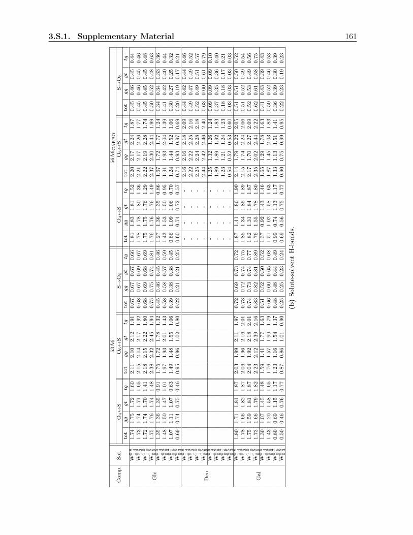
3.S.1. Supplementary Material 161
Com
p.
Sol.
53A
656A
6CARBO
O4↔
SO
6↔
SS→
O5
O4↔
SO
6↔
SS→
O5
tot
gg
gt
tgto
tgg
gt
tgto
tgg
gt
tgto
tgg
gt
tgto
tgg
gt
tgto
tgg
gt
tg
Glc
W0.8
1.4
1.7
41.7
51.7
21.6
02.1
12.1
02.1
21.9
10.6
70.6
70.6
70.6
61.8
11.8
31.8
11.5
22.2
02.1
72.2
41.8
70.4
50.4
60.4
50.4
4W
0.9
1.2
1.7
31.7
41.7
11.6
52.1
52.1
42.1
71.9
20.6
80.6
70.6
90.6
71.7
81.7
81.8
01.3
62.2
12.1
72.2
61.7
70.4
50.4
60.4
50.4
6W
1.0
1.0
1.7
21.7
41.7
01.4
12.1
82.1
52.2
21.8
00.6
80.6
90.6
80.6
91.7
51.7
51.7
61.2
92.2
22.1
92.2
81.7
40.4
50.4
50.4
50.4
8W
1.5
0.5
1.7
51.7
61.7
41.4
82.3
82.3
22.4
51.9
40.7
50.7
50.7
40.8
11.7
61.7
61.7
61.4
92.3
72.3
02.4
41.9
90.5
00.5
20.4
80.6
3W
0.5
1.4
1.3
51.3
61.3
50.9
11.7
51.7
21.7
81.3
20.4
50.4
60.4
50.4
61.2
71.3
61.3
50.8
61.6
71.7
21.7
71.2
40.3
40.3
40.3
30.3
6W
0.8
0.9
1.4
81.5
01.4
71.0
11.9
71.9
32.0
11.4
30.5
80.5
80.5
70.5
91.4
31.5
31.5
00.9
51.9
11.9
32.0
41.3
90.4
10.4
20.4
00.4
4W
0.7
0.6
1.0
71.1
11.0
70.6
31.4
91.4
81.5
51.0
60.3
90.3
80.3
80.4
50.8
61.0
91.0
60.7
01.2
41.4
41.5
21.0
60.3
00.2
70.2
50.3
2W
0.5
0.3
0.6
90.7
40.7
50.4
60.9
50.9
61.0
20.8
00.2
20.2
10.2
10.2
50.6
00.7
40.7
20.5
70.7
40.9
30.9
70.6
90.2
00.1
90.1
70.2
1
Deo
W0.8
1.4
--
--
2.1
62.1
62.1
82.0
90.4
40.4
20.4
40.4
6W
0.9
1.2
--
--
2.2
22.2
22.2
52.1
60.4
90.4
70.4
90.5
2W
1.0
1.0
--
--
2.2
52.2
42.2
82.1
80.5
20.4
90.5
10.5
7W
1.5
0.5
--
--
2.4
42.4
22.4
62.4
00.6
30.6
00.6
10.7
9W
0.5
1.4
--
--
1.2
51.3
21.2
61.2
40.0
90.0
90.0
90.1
0W
0.8
0.9
--
--
1.8
91.8
91.9
21.8
30.3
70.3
50.3
60.4
0W
0.7
0.6
--
--
1.2
31.2
11.2
41.2
30.1
80.1
80.1
70.2
1W
0.5
0.3
--
--
0.5
40.5
20.5
30.6
00.0
30.0
30.0
30.0
3
Gal
W0.8
1.4
1.8
01.7
11.8
11.8
72.0
31.9
92.1
11.9
70.7
20.6
90.7
30.7
21.8
71.4
11.8
61.9
02.1
41.7
92.2
22.0
50.5
10.5
10.5
00.5
2W
0.9
1.2
1.7
81.6
61.8
21.8
72.0
61.9
62.1
62.0
10.7
30.7
20.7
40.7
51.8
51.3
41.8
51.8
92.1
51.7
42.2
42.0
60.5
10.5
20.4
90.5
4W
1.0
1.0
1.7
51.5
91.8
11.8
72.0
41.9
22.1
82.0
10.7
40.7
30.7
40.7
71.8
21.3
11.8
41.8
72.1
71.7
02.2
72.0
90.5
20.5
30.4
90.5
6W
1.5
0.5
1.7
31.6
61.7
91.8
22.2
32.1
22.3
92.1
60.8
30.8
20.8
10.8
91.7
61.5
51.7
81.8
02.3
52.0
22.4
42.2
20.6
20.6
10.5
80.7
5W
0.5
1.4
1.3
01.0
71.4
51.4
81.5
91.4
11.7
71.6
30.5
10.5
20.5
00.5
21.3
70.9
21.4
31.4
61.6
51.2
91.7
81.6
30.4
10.4
30.3
90.4
3W
0.8
0.9
1.4
31.2
01.5
81.6
51.7
61.5
71.9
91.7
90.6
60.6
60.6
50.6
81.5
11.0
21.5
81.6
31.8
71.4
52.0
31.8
30.5
00.5
20.4
60.5
3W
0.7
0.6
0.8
00.6
91.1
51.1
71.2
31.1
61.5
41.3
70.4
80.4
80.4
40.4
90.9
90.7
41.1
31.1
71.3
31.1
31.5
11.4
10.3
60.3
90.3
00.3
9W
0.5
0.3
0.5
00.4
60.7
60.7
70.8
70.8
61.0
10.9
00.2
50.2
50.2
30.2
40.6
90.5
60.7
50.7
70.9
00.7
50.9
90.9
50.2
20.2
30.1
90.2
3
(b)
Solu
te-s
olv
ent
H-b
on
ds.

162 Chapter 3. Monosaccharides
Table
3.S.11:
Det
aile
dH
-bon
ds
anal
ysi
sfo
rth
eth
ree
com
pou
nd
sin
the
seri
esSP h
of
arti
fici
also
lven
tsat
298.
15K
and
998.
3kg·m−
3.
Th
eva
lues
are
calc
ula
ted
asav
erages
over
the
40n
sp
has
eof
the
diff
eren
tL
EU
Ssi
mu
lati
ons.
Th
eco
mp
oun
ds
con
sid
ered
are
Glc
,D
eoan
dG
al(F
igu
re3.
1),
alon
gth
ese
ries
SP h
ofar
tifi
cial
solv
ents
(Tab
le3.3
)in
ord
erof
dec
reas
ing
H-b
ond
ing
cap
acit
yat
wat
er-l
ike
die
lect
ric
per
mit
tivit
y.T
he
forc
efi
eld
sco
nsi
der
edar
eth
e53
A6
forc
efi
eld
244
and
56A
6 CA
RB
Ofo
rce
fiel
d245.
Ina,
the
aver
age
nu
mb
ers
ofin
tram
olec
ula
rH
4→
O6,
H6→
O4
and
H6→
O5
H-b
ond
sar
ere
por
ted
.In
b,
the
aver
age
nu
mb
ers
ofso
lute
-sol
vent
O4↔
S,
O6↔
San
dS→
O5
H-b
ond
sar
ere
por
ted
.T
he
aver
age
nu
mb
ers
are
calc
ula
ted
eith
erov
erth
een
tire
sim
ula
tion
(N)
orov
erth
eth
ree
can
onic
alro
tam
ers
sep
arat
ely,
i.e.
asNgg,Ngt
andNtg
.T
he
dat
ais
illu
stra
ted
grap
hic
all
yin
Su
pp
l.M
at.
Fig
ure
s3.
S.6
and
3.S
.10.
(a)
Intr
am
ole
cula
rH
-bon
ds
Com
p.
Sol.
53A
656A
6CARBO
H4→
O6
H6→
O4
H6→
O5
H4→
O6
H6→
O4
H6→
O5
tot
gg
gt
tgto
tgg
gt
tgto
tgg
gt
tgto
tgg
gt
tgto
tgg
gt
tgto
tgg
gt
tg
Glc
W1.1
0.9
0.0
00.0
00.0
00.3
10.0
00.0
00.0
00.2
40.0
30.0
30.0
30.0
00.0
20.0
00.0
00.4
00.0
10.0
00.0
00.2
70.0
90.0
90.1
00.0
0W
1.0
1.0
0.0
00.0
00.0
00.2
60.0
00.0
00.0
00.2
00.0
30.0
30.0
30.0
00.0
20.0
00.0
00.4
20.0
10.0
00.0
00.2
40.0
70.0
70.0
80.0
0W
0.8
1.1
0.0
00.0
00.0
00.3
50.0
00.0
00.0
00.2
10.0
30.0
30.0
30.0
00.0
30.0
00.0
00.4
30.0
20.0
00.0
00.2
90.0
80.0
80.0
90.0
0W
0.7
1.2
0.0
00.0
00.0
00.3
60.0
00.0
00.0
00.2
20.0
30.0
30.0
40.0
00.0
30.0
00.0
00.4
50.0
20.0
00.0
00.3
10.0
80.0
80.0
90.0
0W
0.6
1.4
0.0
00.0
00.0
00.3
20.0
00.0
00.0
00.2
50.0
30.0
30.0
30.0
00.0
30.0
00.0
00.4
70.0
20.0
00.0
00.2
70.0
70.0
70.0
80.0
0W
0.5
1.5
0.0
00.0
00.0
00.4
60.0
00.0
00.0
00.3
00.0
40.0
40.0
40.0
00.0
50.0
10.0
00.5
20.0
40.0
00.0
00.3
60.1
00.1
00.1
20.0
0
Deo
W1.1
0.9
--
--
--
--
0.0
80.1
00.0
80.0
0W
1.0
1.0
--
--
--
--
0.0
60.0
90.0
60.0
0W
0.8
1.1
--
--
--
--
0.0
50.0
80.0
60.0
0W
0.7
1.2
--
--
--
--
0.0
60.0
80.0
70.0
0W
0.6
1.4
--
--
--
--
0.0
50.0
80.0
60.0
0W
0.5
1.5
--
--
--
--
0.0
70.1
10.0
90.0
0
Gal
W1.1
0.9
0.0
90.2
60.0
00.0
00.0
50.1
50.0
00.0
00.0
20.0
20.0
20.0
00.0
40.4
70.0
00.0
00.0
20.2
50.0
00.0
00.0
60.0
60.1
00.0
0W
1.0
1.0
0.0
90.2
50.0
00.0
00.0
40.1
00.0
00.0
00.0
10.0
20.0
20.0
00.0
30.5
10.0
00.0
00.0
10.2
00.0
00.0
00.0
50.0
40.0
80.0
0W
0.8
1.1
0.0
70.2
30.0
00.0
00.0
60.1
70.0
00.0
00.0
10.0
10.0
20.0
00.0
40.5
40.0
00.0
00.0
20.2
60.0
00.0
00.0
40.0
30.0
80.0
0W
0.7
1.2
0.0
90.2
80.0
00.0
00.0
60.1
80.0
00.0
00.0
10.0
20.0
20.0
00.0
40.5
30.0
00.0
00.0
20.2
90.0
00.0
00.0
40.0
30.0
80.0
0W
0.6
1.4
0.0
90.3
00.0
00.0
00.0
40.1
40.0
00.0
00.0
10.0
10.0
20.0
00.0
40.5
50.0
00.0
00.0
20.2
70.0
00.0
00.0
40.0
30.0
80.0
0W
0.5
1.5
0.1
10.3
50.0
00.0
00.0
80.2
40.0
00.0
00.0
10.0
10.0
30.0
00.0
60.6
00.0
00.0
00.0
30.3
10.0
00.0
00.0
60.0
20.1
20.0
0

3.S.1. Supplementary Material 163
Com
p.
Sol.
53A
656A
6CARBO
O4↔
SO
6↔
SS→
O5
O4↔
SO
6↔
SS→
O5
tot
gg
gt
tgto
tgg
gt
tgto
tgg
gt
tgto
tgg
gt
tgto
tgg
gt
tgto
tgg
gt
tg
Glc
W1.1
0.9
1.7
31.7
31.7
21.3
62.1
72.1
52.2
01.7
40.6
80.6
80.6
90.7
31.7
61.7
71.7
91.2
92.2
02.1
72.2
71.7
20.4
30.4
40.4
10.4
9W
1.0
1.0
1.7
21.7
41.7
01.4
12.1
82.1
52.2
21.8
00.6
80.6
90.6
80.6
91.7
51.7
81.7
61.2
92.2
22.1
92.2
81.7
40.4
50.4
50.4
50.4
8W
0.8
1.1
1.6
31.6
41.6
11.3
02.0
52.0
52.0
61.6
70.6
30.6
30.6
20.6
31.6
31.6
81.6
51.1
72.0
92.0
52.1
61.5
50.4
40.4
60.4
40.4
4W
0.7
1.2
1.5
61.5
71.5
41.2
31.9
71.9
51.9
91.6
10.5
80.5
80.5
80.5
51.5
51.6
01.5
71.1
21.9
91.9
62.0
51.4
90.4
10.4
20.4
00.4
3W
0.6
1.4
1.5
21.5
31.5
21.2
21.9
01.8
81.9
21.5
60.5
30.5
30.5
30.5
21.5
11.5
61.5
31.0
81.9
11.8
81.9
61.4
70.3
90.4
00.3
90.4
0W
0.5
1.5
1.4
11.4
31.4
01.0
01.7
91.7
71.8
11.3
90.4
70.4
60.4
70.4
61.3
61.4
31.4
00.9
11.7
61.7
61.8
31.3
00.3
50.3
50.3
40.3
6
Deo
W1.1
0.9
--
--
2.2
62.2
42.2
82.1
80.5
30.5
10.5
20.6
0W
1.0
1.0
--
--
2.2
52.2
42.2
82.1
80.5
20.4
90.5
00.5
7W
0.8
1.1
--
--
2.0
32.0
22.0
61.9
60.4
00.3
90.2
80.4
2W
0.7
1.2
--
--
1.8
01.8
11.5
11.4
80.3
10.3
00.1
60.3
2W
0.6
1.4
--
--
1.6
01.6
01.3
31.2
80.2
00.2
00.0
90.2
0W
0.5
1.5
--
--
1.2
91.3
01.2
91.2
20.0
90.0
90.0
40.1
0
Gal
W1.1
0.9
1.7
41.5
61.8
21.8
72.0
31.8
82.1
72.0
20.7
40.7
40.7
20.7
81.8
01.3
31.8
41.8
62.1
41.7
12.2
42.0
80.5
20.5
10.4
80.5
8W
1.0
1.0
1.7
51.5
91.8
11.8
72.0
41.9
22.1
82.0
10.7
40.7
30.7
40.7
71.8
21.3
11.8
41.8
72.1
71.7
02.2
72.0
90.5
20.5
30.4
90.5
6W
0.8
1.1
1.6
61.4
91.7
01.7
71.9
41.8
22.0
61.8
90.6
90.6
90.6
90.7
01.7
11.1
81.7
31.7
62.0
11.5
62.1
31.9
50.5
30.5
30.5
20.5
4W
0.7
1.2
1.5
71.4
01.6
41.6
71.8
51.7
21.9
71.8
10.6
40.6
40.6
50.6
31.6
31.1
11.6
51.6
91.9
31.4
92.0
41.8
70.5
00.4
90.4
80.5
2W
0.6
1.4
1.5
41.3
71.5
91.6
41.8
01.6
91.9
11.7
60.5
90.6
00.6
00.5
91.5
91.0
61.6
01.6
51.8
51.4
71.9
51.8
00.4
70.4
60.4
60.4
8W
0.5
1.5
1.4
01.1
91.4
81.5
31.6
61.5
01.7
91.6
60.5
30.5
30.5
30.5
11.4
30.9
31.4
61.5
11.7
01.3
21.8
11.6
80.4
20.4
30.4
00.4
4
(b)
Solu
te-s
olv
ent
H-b
ond
s.

164 Chapter 3. Monosaccharides
Table
3.S.12:
Det
aile
dH
-bon
ds
anal
ysi
sfo
rth
eth
ree
com
pou
nd
sin
the
seri
esSp h
of
arti
fici
also
lven
tsat
298.
15K
and
998.
3kg·
m−
3.
Th
eva
lues
are
calc
ula
ted
asav
erag
esov
erth
e40
ns
ph
ase
ofth
ed
iffer
ent
LE
US
sim
ula
tion
s.T
he
com
pou
nd
sco
nsi
der
edar
eG
lc,
Deo
and
Gal
(Fig
ure
3.1)
,al
ong
the
seri
esSp h
ofar
tifi
cial
solv
ents
(Tab
le3.
3)in
ord
erof
dec
reas
ing
H-b
ond
ing
cap
acit
yat
low
die
lect
ric
per
mit
tivit
y.T
he
forc
efi
eld
sco
nsi
der
edar
eth
e53
A6
forc
efi
eld
244
(lef
t)an
d56
A6
CA
RB
Ofo
rce
fiel
d245
(rig
ht)
.In
a,th
eav
erage
nu
mb
ers
ofin
tram
olec
ula
rH
4→
O6,
H6→
O4
and
H6→
O5
H-b
ond
sar
ere
por
ted
,w
her
eS
isa
solv
ent
don
oror
acce
pto
rsi
te.
Inb
,th
eav
erag
enu
mb
ers
ofso
lute
-sol
vent
O4↔
S,
O6↔
San
dS→
O5
H-b
ond
sar
ere
por
ted
.T
he
aver
age
nu
mb
ers
are
calc
ula
ted
eith
erov
erth
een
tire
sim
ula
tion
(N)
orov
erth
eth
ree
can
onic
alro
tam
ers
sep
arat
ely,
i.e.
asNgg,Ngt
andNtg
.T
he
dat
ais
illu
stra
ted
grap
hic
ally
inS
up
pl.
Mat
.F
igu
res
3.S
.7an
d3.
S.1
1.
(a)
Intr
am
ole
cula
rH
-bon
ds
Com
p.
Sol.
53A
656A
6CARBO
H4→
O6
H6→
O4
H6→
O5
H4→
O6
H6→
O4
H6→
O5
tot
gg
gt
tgto
tgg
gt
tgto
tgg
gt
tgto
tgg
gt
tgto
tgg
gt
tgto
tgg
gt
tg
Glc
W1.5
0.4
0.0
00.0
00.0
00.6
40.0
00.0
00.0
00.2
40.1
30.1
20.1
40.0
00.0
50.0
10.0
00.4
90.0
40.0
00.0
00.4
10.2
30.2
40.2
60.0
0W
1.2
0.5
0.0
10.0
00.0
00.6
80.0
00.0
00.0
00.2
40.1
10.1
10.1
20.0
00.1
30.0
10.0
00.5
60.0
90.0
10.0
00.3
90.1
90.2
10.2
60.0
0W
1.1
0.5
0.0
10.0
00.0
00.7
50.0
00.0
00.0
00.2
10.1
20.1
20.1
40.0
00.1
70.0
10.0
00.5
20.1
50.0
10.0
00.4
50.1
70.2
20.2
80.0
0W
0.8
0.7
0.0
10.0
00.0
00.7
30.0
00.0
00.0
00.2
30.1
10.1
10.1
20.0
00.1
80.0
10.0
00.4
90.1
70.0
10.0
00.4
80.1
50.2
00.2
50.0
0W
0.6
0.9
0.0
10.0
00.0
00.7
70.0
00.0
00.0
00.2
00.1
10.1
00.1
20.0
00.2
20.0
20.0
00.5
50.1
70.0
10.0
00.4
30.1
40.2
00.2
50.0
0W
0.4
1.3
0.0
20.0
00.0
00.8
00.0
00.0
00.0
00.1
80.1
10.1
10.1
30.0
00.2
30.0
20.0
00.5
20.2
10.0
10.0
00.4
60.1
40.2
10.2
70.0
0
Deo
W1.5
0.4
--
--
--
--
0.2
20.2
90.2
50.0
0W
1.2
0.5
--
--
--
--
0.1
80.2
50.2
20.0
0W
1.1
0.5
--
--
--
--
0.2
00.3
70.2
40.0
0W
0.8
0.7
--
--
--
--
0.1
70.2
40.2
20.0
0W
0.6
0.9
--
--
--
--
0.1
80.2
50.2
30.0
0W
0.4
1.3
--
--
--
--
0.1
80.2
60.2
40.0
0
Gal
W1.5
0.4
0.2
70.4
90.0
00.0
10.1
10.2
00.0
00.0
10.0
50.0
50.0
90.0
00.0
70.4
80.0
00.0
10.0
60.3
70.0
00.0
10.1
80.0
90.2
80.0
0W
1.2
0.5
0.3
10.5
30.0
00.0
10.1
60.2
70.0
00.0
10.0
40.0
30.0
80.0
00.1
30.5
30.0
00.0
10.0
90.4
00.0
00.0
00.1
40.0
50.2
70.0
0W
1.1
0.5
0.3
80.5
80.0
00.0
10.1
90.2
90.0
00.0
10.0
30.0
20.0
90.0
00.1
60.5
30.0
00.0
10.1
30.4
30.0
00.0
10.1
30.0
40.2
80.0
0W
0.8
0.7
0.3
40.5
50.0
00.0
10.2
00.3
20.0
00.0
10.0
30.0
20.0
70.0
00.1
60.5
30.0
00.0
10.1
30.4
30.0
00.0
10.1
20.0
30.2
70.0
0W
0.6
0.9
0.3
70.5
80.0
00.0
10.2
00.3
10.0
00.0
10.0
30.0
20.0
80.0
00.1
50.5
20.0
00.0
10.1
40.4
60.0
00.0
10.1
10.0
30.2
60.0
0W
0.4
1.3
0.4
10.6
30.0
00.0
10.1
90.2
80.0
00.0
10.0
30.0
20.0
80.0
00.1
80.5
40.0
00.0
10.1
50.4
40.0
00.0
10.1
10.0
30.2
90.0
0

3.S.1. Supplementary Material 165
Com
p.
Sol.
53A
656A
6CARBO
O4↔
SO
6↔
SS→
O5
O4↔
SO
6↔
SS→
O5
tot
gg
gt
tgto
tgg
gt
tgto
tgg
gt
tgto
tgg
gt
tgto
tgg
gt
tgto
tgg
gt
tg
Glc
W1.5
0.4
1.8
51.8
51.8
41.4
32.4
32.4
02.4
91.8
40.8
20.8
30.8
00.8
51.8
51.9
01.9
01.4
42.4
12.3
92.5
11.9
10.5
40.5
60.5
20.6
5W
1.2
0.5
1.5
81.5
91.5
81.0
42.1
72.1
42.2
11.4
80.6
90.7
00.6
80.7
51.5
01.6
31.6
21.0
52.0
62.1
32.2
41.5
40.4
70.4
80.4
40.5
4W
1.1
0.5
1.4
41.4
61.4
40.9
12.0
01.9
72.0
61.3
60.6
30.6
30.6
30.6
81.3
11.4
91.4
90.9
41.8
51.9
72.0
81.4
40.4
30.4
30.4
00.4
9W
0.8
0.7
1.3
01.3
21.3
00.7
81.7
81.7
61.8
21.2
50.5
00.5
10.5
00.5
41.1
31.3
31.3
00.8
21.6
11.7
31.8
41.2
50.3
70.3
60.3
40.4
1W
0.6
0.9
1.2
01.2
31.1
90.6
81.6
41.6
21.6
71.1
70.4
30.4
30.4
20.4
61.0
11.2
01.1
80.7
31.4
31.5
71.6
51.1
40.3
20.3
00.2
90.3
5W
0.4
1.3
1.1
01.1
21.1
00.6
11.4
81.4
81.5
01.1
20.3
50.3
40.3
60.3
80.9
01.1
01.0
70.6
81.2
81.4
21.4
81.0
50.2
70.2
70.2
50.2
9
Deo
W1.5
0.4
--
--
2.5
02.5
22.5
22.4
20.6
70.6
40.6
50.8
0W
1.2
0.5
--
--
2.2
52.2
92.2
92.1
60.5
90.5
70.5
70.6
8W
1.1
0.5
--
--
2.1
02.1
32.1
32.0
20.5
20.4
90.5
00.6
1W
0.8
0.7
--
--
1.6
51.6
71.6
71.6
20.3
10.2
90.2
90.3
5W
0.6
0.9
--
--
1.2
41.2
41.2
41.2
50.1
40.1
30.1
30.1
5W
0.4
1.3
--
--
0.8
80.8
50.8
60.9
20.0
30.0
20.0
20.0
3
Gal
W1.5
0.4
1.7
61.6
21.9
01.9
52.2
12.0
62.4
62.2
40.8
90.8
90.8
70.9
41.8
51.5
01.9
11.9
32.3
71.9
82.4
92.2
90.6
50.6
60.6
00.7
6W
1.2
0.5
1.4
31.2
41.6
71.7
41.8
61.6
92.1
91.9
50.8
00.8
00.7
60.8
31.5
71.1
31.7
01.7
22.0
31.6
42.2
42.0
20.5
60.6
10.5
00.6
2W
1.1
0.5
1.2
51.0
71.5
41.5
91.6
81.5
32.0
41.8
00.7
30.7
40.7
00.7
71.4
01.0
01.5
51.5
81.8
51.4
92.0
91.8
80.5
20.5
60.4
50.5
7W
0.8
0.7
1.1
30.9
41.3
91.4
31.5
11.3
71.8
21.6
40.6
10.6
10.5
80.6
11.2
50.8
91.3
91.4
21.6
21.3
21.8
31.6
60.4
50.4
80.3
90.4
8W
0.6
0.9
1.0
10.8
41.2
81.3
31.3
91.2
91.6
61.4
90.5
10.5
10.4
80.5
21.1
50.8
31.2
61.3
01.4
71.1
81.6
51.5
30.3
80.4
10.3
40.4
1W
0.4
1.3
0.9
10.7
51.1
81.2
21.2
81.1
81.5
11.3
90.4
30.4
40.4
00.4
31.0
20.7
41.1
61.1
81.3
21.0
91.4
61.4
00.3
30.3
50.2
80.3
7
(b)
Solu
te-s
olv
ent
H-b
on
ds.

166 Chapter 3. Monosaccharides
Figure 3.S.1: Normalized probability distributions around the dihedral angle ω for thethree compounds considered in the series SHp and Shp of artificial solvents at 298.15 K and998.3 kg·m−3. The values are calculated as reweighted averages over the 40 ns US phase ofthe different LEUS simulations using a bin size of 2. The different panels from left to rightcorrespond to Glc, Deo and Gal (Figure 3.1), and from top to bottom to the series of artificialsolvents (Table 3.3) SHp with decreasing permittivity at water-like H-bonding capacity (four
upper panels) and Shp with decreasing permittivity at lower H-bonding capacity (four lowerpanels). The black curves correspond to the 53A6 force field244 and the red curves to the56A6CARBO force field245. The simulations of Deo with 53A6 are omitted due to ambiguoustorsional potential definitions. See Figure 3.3 for corresponding results with the physicalsolvents and Suppl. Mat. Figures 3.S.2 and 3.S.3 for the other series of artificial solvents.

3.S.1. Supplementary Material 167
Figure 3.S.2: Normalized probability distributions around the dihedral angle ω for thethree compounds considered in the series SPh of artificial solvents at 298.15 K and 998.3kg·m−3. The values are calculated as reweighted averages over the 40 ns US phase of thedifferent LEUS simulations using a bin size of 2. The different panels from left to rightcorrespond to Glc, Deo and Gal (Figure 3.1), and from top to bottom to the series of artificialsolvents (Table 3.3) SPh with decreasing H-bonding capacity at water-like permittivity. Theblack curves correspond to the 53A6 force field244 and the red curves to the 56A6CARBO
force field245. The simulations of Deo with 53A6 are omitted due to ambiguous torsionalpotential definitions. See Figure 3.3 for corresponding results with the physical solvents andSuppl. Mat. Figures 3.S.1 and 3.S.3 for the other series of artificial solvents.

168 Chapter 3. Monosaccharides
Figure 3.S.3: Normalized probability distributions around the dihedral angle ω for thethree compounds considered in the series Sph of artificial solvents at 298.15 K and 998.3kg·m−3. The values are calculated as reweighted averages over the 40 ns US phase ofthe different LEUS simulations using a bin size of 2. The different panels from left toright correspond to Glc, Deo and Gal (Figure 3.1), and from top to bottom to the seriesof artificial solvents (Table 3.3) Sph with decreasing H-bonding capacity at low permittivity.The black curves correspond to the 53A6 force field244 and the red curves to the 56A6CARBO
force field245. The simulations of Deo with 53A6 are omitted due to ambiguous torsionalpotential definitions. See Figure 3.3 for corresponding results with the physical solvents andSuppl. Mat. Figures 3.S.1 and 3.S.2 for the other series of artificial solvents.
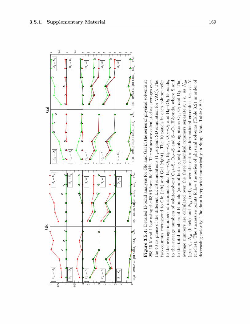
3.S.1. Supplementary Material 169
0.51
H4
→ O
6
G
lc
O4
↔ O
6
0.51
H6
→ O
4H
6→
O5
123O
4↔
SO
4 tot
123O
6↔
SO
6 tot
H2O
DM
SO C
H3O
HC
HC
l 3C
Cl 4
VA
C0123
S →
O5
H2O
DM
SO C
H3O
HC
HC
l 3C
Cl 4
VA
C
O5 to
t
H4
→ O
6
G
al
0.5
1O
4↔
O6
H6
→ O
4
0.5
1H
6→
O5
O4
↔ S
123O
4 tot
O6
↔ S
123O
6 tot
H2O
DM
SO C
H3O
HC
HC
l 3C
Cl 4
VA
C
S →
O5
H2O
DM
SO C
H3O
HC
HC
l 3C
Cl 4
VA
C0123
O5 to
t
Figure
3.S.4:
Det
aile
dH
-bon
dan
alysi
sfo
rG
lcan
dG
alin
the
seri
esof
physi
calso
lven
tsat
298.
15
Kan
d1
bar
usi
ng
the
53A
6fo
rce
fiel
d244.
Th
eva
lues
are
calc
ula
ted
as
aver
ages
over
the
40n
sp
has
eof
the
diff
eren
tL
EU
Ssi
mu
lati
ons
(1µ
sp
lain
SD
sim
ula
tion
for
VA
C).
Th
etw
oco
lum
ns
corr
esp
on
dto
Glc
(lef
t)an
dG
al(r
ight)
.T
he
10p
anel
sin
each
colu
mn
refe
rto
the
aver
age
nu
mb
ers
ofin
tram
olec
ula
rH
4→
O6,
H6→
O4,
O4↔
O6
and
H6→
O5
H-b
on
ds,
toth
eav
erag
enu
mb
ers
ofso
lute
-sol
vent
O4↔
S,
O6↔
San
dS→
O5
H-b
ond
s,w
her
eS
an
dto
the
tota
lnu
mb
ers
ofH
-bon
ds
(sum
ofb
oth
typ
es)
invo
lvin
gat
oms
O4,
O6
and
O5.
Th
eav
erag
enu
mb
ers
are
calc
ula
ted
over
the
thre
eca
non
ical
rota
mer
sse
par
atel
y,i.e.
asNgg
(gre
en),Ngt
(bla
ck)
an
dNtg
(red
),or
over
the
enti
reco
nfo
rmat
ion
alen
sem
ble
,i.e.
asN
(cir
cles
).T
he
succ
essi
vep
oints
foll
owth
ese
ries
ofp
hysi
cal
solv
ents
(Tab
le3.
2)
inor
der
of
dec
reas
ing
pola
rity
.T
he
dat
ais
rep
orte
dnum
eric
ally
inS
up
p.
Mat
.T
able
3.S
.9.

170 Chapter 3. Monosaccharides
0.51
H4
→ O
6
G
lc
O4
↔ O
6
0.51
H6
→ O
4H
6→
O5
123O
4↔
SO
4 tot
123O
6↔
SO
6 tot
W1.
40.8
W1.
20.9
W1.
01.0
W0.
51.5
W1.
40.5
W0.
90.8
W0.
60.7
W0.
30.5
0123S
→ O
5
W1.
40.8
W1.
20.9
W1.
01.0
W0.
51.5
W1.
40.5
W0.
90.8
W0.
60.7
W0.
30.5
O5 to
t
H4
→ O
6
G
al
0.5
1O
4↔
O6
H6
→ O
4
0.5
1H
6→
O5
O4
↔ S
123O
4 tot
O6
↔ S
123O
6 tot
W1.
40.8
W1.
20.9
W1.
01.0
W0.
51.5
W1.
40.5
W0.
90.8
W0.
60.7
W0.
30.5
S →
O5
W1.
40.8
W1.
20.9
W1.
01.0
W0.
51.5
W1.
40.5
W0.
90.8
W0.
60.7
W0.
30.5
0123O
5 tot
Figure
3.S.5:
Det
ail
edH
-bon
dan
alysi
sfo
rG
lcan
dG
alin
the
seri
esSH p
an
dSh p
of
art
ifici
al
solv
ents
at
298.
15K
and
998.
3kg·m−
3u
sin
gth
e53
A6
forc
efi
eld
244.
Th
eva
lues
are
calc
ula
ted
asav
erage
sov
erth
e40
ns
ph
ase
ofth
ed
iffer
ent
LE
US
sim
ula
tion
s.T
he
two
colu
mn
sco
rres
pon
dto
Glc
(lef
t)an
dG
al(r
ight)
.T
he
10p
anel
sin
each
colu
mn
refe
rto
the
aver
age
nu
mb
ers
of
intr
amol
ecu
lar
H4→
O6,
H6→
O4,
O4↔
O6
and
H6→
O5
H-b
ond
s,to
the
aver
age
nu
mb
ers
ofso
lute
-sol
vent
O4↔
S,
O6↔
San
dS→
O5
H-b
ond
s,w
her
eS
isa
solv
ent
don
oror
acce
pto
rsi
te,
an
dto
the
tota
lnu
mb
ers
ofH
-bon
ds
(su
mof
bot
hty
pes
)in
volv
ing
ato
ms
O4,O
6an
dO
5.
Th
eav
erag
enu
mb
ers
are
calc
ula
ted
over
the
thre
eca
non
ical
rota
mer
sse
par
ate
ly,i.e.
asNgg
(gre
en),Ngt
(bla
ck)
andNtg
(red
),or
over
the
enti
reco
nfo
rmati
on
al
ense
mb
le,i.e.
asN
(cir
cles
).T
he
succ
essi
vep
oints
foll
owth
ese
riesSH p
andSh p
ofart
ifici
al
solv
ents
(Tab
le3.3
)in
ord
erof
dec
reas
ing
die
lect
ric
per
mit
tivit
yat
wat
er-l
ike
or
low
erH
-b
on
din
gca
pac
ity,
resp
ecti
vel
y.T
he
dat
ais
rep
orte
dnu
mer
ical
lyin
Su
pp
.M
at.
Tab
le3.S
.10.

3.S.1. Supplementary Material 171
0.51
H4
→ O
6
G
lc
O4
↔ O
6
0.51
H6
→ O
4H
6→
O5
123O
4↔
SO
4 tot
123O
6↔
SO
6 tot
W0.
91.1
W1.
01.0
W1.
10.8
W1.
20.7
W1.
40.6
W1.
50.5
0123S
→ O
5
W0.
91.1
W1.
01.0
W1.
10.8
W1.
20.7
W1.
40.6
W1.
50.5
O5 to
t
H4
→ O
6
G
al
0.5
1O
4↔
O6
H6
→ O
4
0.5
1H
6→
O5
O4
↔ S
123O
4 tot
O6
↔ S
123O
6 tot
W0.
91.1
W1.
01.0
W1.
10.8
W1.
20.7
W1.
40.6
W1.
50.5
S →
O5
W0.
91.1
W1.
01.0
W1.
10.8
W1.
20.7
W1.
40.6
W1.
50.5
0123O
5 tot
Figure
3.S.6:
Det
ail
edH
-bon
dan
alysi
sfo
rG
lcan
dG
alin
the
seri
esSP h
ofar
tifi
cial
solv
ents
at
298.
15
Kan
d99
8.3
kg·
m−
3u
sin
gth
e53
A6
forc
efi
eld
244.
Th
eva
lues
are
calc
ula
ted
as
aver
age
sov
erth
e40
ns
ph
ase
ofth
ed
iffer
ent
LE
US
sim
ula
tion
s.T
he
two
colu
mn
sco
rres
pon
dto
Glc
(lef
t)an
dG
al(r
ight)
.T
he
10p
anel
sin
each
colu
mn
refe
rto
the
aver
age
nu
mb
ers
of
intr
amole
cula
rH
4→
O6,
H6→
O4,
O4↔
O6
and
H6→
O5
H-b
ond
s,to
the
aver
age
nu
mb
ers
of
solu
te-s
olv
ent
O4↔
S,
O6↔
San
dS→
O5
H-b
ond
s,w
her
eS
isa
solv
ent
don
or
or
acc
epto
rsi
te,
an
dto
the
tota
lnu
mb
ers
ofH
-bon
ds
(su
mof
bot
hty
pes
)in
vol
vin
gato
ms
O4,
O6
an
dO
5.
Th
eav
erag
enu
mb
ers
are
calc
ula
ted
over
the
thre
eca
non
ical
rota
mer
sse
para
tely
,i.e.
asNgg
(gre
en),Ngt
(bla
ck)
andNtg
(red
),or
over
the
enti
reco
nfo
rmati
on
al
ense
mb
le,i.e.
asN
(cir
cles
).T
he
succ
essi
vep
oints
foll
owth
ese
riesSP h
ofar
tifi
cial
solv
ent
(Tab
le3.3
)in
ord
erof
dec
reas
ing
H-b
ond
ing
cap
acit
yat
wat
er-l
ike
die
lect
ric
per
mit
tivit
y.T
he
data
isre
por
ted
nu
mer
ical
lyin
Su
pp
.M
at.
Tab
le3.
S.1
1.

172 Chapter 3. Monosaccharides
0.51
H4
→ O
6
G
lc
O4
↔ O
6
0.51
H6
→ O
4H
6→
O5
123O
4↔
SO
4 tot
123O
6↔
SO
6 tot
W0.
41.5
W0.
51.2
W0.
51.1
W0.
70.8
W0.
90.6
W1.
30.4
0123S
→ O
5
W0.
41.5
W0.
51.2
W0.
51.1
W0.
70.8
W0.
90.6
W1.
30.4
O5 to
t
H4
→ O
6
G
al
0.5
1O
4↔
O6
H6
→ O
4
0.5
1H
6→
O5
O4
↔ S
123O
4 tot
O6
↔ S
123O
6 tot
W0.
41.5
W0.
51.2
W0.
51.1
W0.
70.8
W0.
90.6
W1.
30.4
S →
O5
W0.
41.5
W0.
51.2
W0.
51.1
W0.
70.8
W0.
90.6
W1.
30.4
0123O
5 tot
Figure
3.S.7:
Det
aile
dH
-bon
dan
alysi
sfo
rG
lcan
dG
alin
the
seri
esSp h
ofart
ifici
also
lven
tsat
298.
15
Kan
d99
8.3
kg·
m−
3u
sin
gth
e53
A6
forc
efi
eld
244.
Th
eva
lues
are
calc
ula
ted
as
aver
age
sov
erth
e40
ns
ph
ase
ofth
ed
iffer
ent
LE
US
sim
ula
tion
s.T
he
two
colu
mn
sco
rres
pon
dto
Glc
(lef
t)an
dG
al(r
ight)
.T
he
10p
anel
sin
each
colu
mn
refe
rto
the
aver
age
nu
mb
ers
of
intr
amole
cula
rH
4→
O6,
H6→
O4,
O4↔
O6
and
H6→
O5
H-b
ond
s,to
the
aver
age
nu
mb
ers
of
solu
te-s
olv
ent
O4↔
S,
O6↔
San
dS→
O5
H-b
ond
s,w
her
eS
isa
solv
ent
don
or
or
acc
epto
rsi
te,
an
dto
the
tota
lnu
mb
ers
ofH
-bon
ds
(su
mof
bot
hty
pes
)in
vol
vin
gato
ms
O4,
O6
an
dO
5.
Th
eav
erag
enu
mb
ers
are
calc
ula
ted
over
the
thre
eca
non
ical
rota
mer
sse
para
tely
,i.e.
asNgg
(gre
en),Ngt
(bla
ck)
andNtg
(red
),or
over
the
enti
reco
nfo
rmati
on
al
ense
mb
le,i.e.
asN
(cir
cles
).T
he
succ
essi
vep
oints
foll
owth
ese
riesSp h
ofar
tifi
cial
solv
ent
(Tab
le3.
3)
inord
erof
dec
reas
ing
H-b
ond
ing
cap
acit
yat
low
die
lect
ric
per
mit
tivit
y.T
he
data
isre
port
ednu
mer
ical
lyin
Su
pp
.M
at.
Tab
le3.
S.1
2.
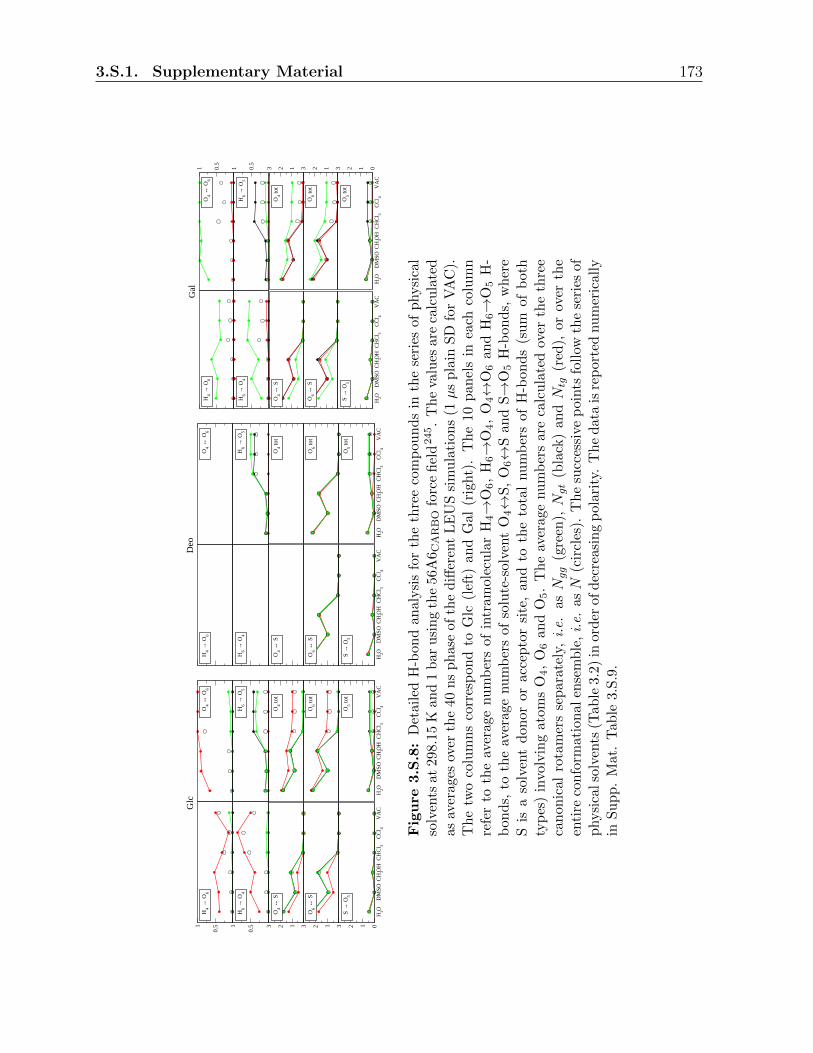
3.S.1. Supplementary Material 173
0.51
H4
→ O
6
G
lc
O4
↔ O
6
0.51
H6
→ O
4H
6→
O5
123O
4↔
SO
4 tot
123O
6↔
SO
6 tot
H2O
DM
SO C
H3O
HC
HC
l 3C
Cl 4
VA
C0123
S →
O5
H2O
DM
SO C
H3O
HC
HC
l 3C
Cl 4
VA
C
O5 to
t
H4
→ O
6
D
eo
O4
↔ O
6
H6
→ O
4H
6→
O5
O4
↔ S
O4 to
t
O6
↔ S
O6 to
t
H2O
DM
SO C
H3O
HC
HC
l 3C
Cl 4
VA
C
S →
O5
H2O
DM
SO C
H3O
HC
HC
l 3C
Cl 4
VA
C
O5 to
t
H4
→ O
6
G
al
0.5
1O
4↔
O6
H6
→ O
4
0.5
1H
6→
O5
O4
↔ S
123O
4 tot
O6
↔ S
123O
6 tot
H2O
DM
SO C
H3O
HC
HC
l 3C
Cl 4
VA
C
S →
O5
H2O
DM
SO C
H3O
HC
HC
l 3C
Cl 4
VA
C0123
O5 to
t
Figure
3.S.8:
Det
ail
edH
-bon
dan
alysi
sfo
rth
eth
ree
com
pou
nd
sin
the
seri
esof
physi
cal
solv
ents
at298
.15
Kan
d1
bar
usi
ng
the
56A
6C
AR
BO
forc
efi
eld
245.
Th
eva
lues
are
calc
ula
ted
as
aver
ages
over
the
40n
sp
has
eof
the
diff
eren
tL
EU
Ssi
mu
lati
ons
(1µ
spla
inS
Dfo
rV
AC
).T
he
two
colu
mns
corr
esp
ond
toG
lc(l
eft)
and
Gal
(rig
ht)
.T
he
10p
anel
sin
each
colu
mn
refe
rto
the
aver
age
nu
mb
ers
ofin
tram
olec
ula
rH
4→
O6,
H6→
O4,
O4↔
O6
an
dH
6→
O5
H-
bon
ds,
toth
eav
erage
nu
mb
ers
ofso
lute
-sol
vent
O4↔
S,
O6↔
San
dS→
O5
H-b
on
ds,
wh
ere
Sis
aso
lven
td
onor
or
acce
pto
rsi
te,
and
toth
eto
tal
nu
mb
ers
ofH
-bon
ds
(su
mof
both
typ
es)
invo
lvin
gato
ms
O4,
O6
and
O5.
Th
eav
erag
enu
mb
ers
are
calc
ula
ted
over
the
thre
eca
non
ical
rota
mer
sse
par
atel
y,i.e.
asNgg
(gre
en),Ngt
(bla
ck)
andNtg
(red
),or
over
the
enti
reco
nfo
rmat
ional
ense
mb
le,i.e.
asN
(cir
cles
).T
he
succ
essi
vep
oints
foll
owth
ese
ries
of
physi
calso
lven
ts(T
ab
le3.
2)in
order
ofd
ecre
asin
gp
olar
ity.
Th
ed
ata
isre
por
ted
nu
mer
icall
yin
Su
pp
.M
at.
Tab
le3.S
.9.

174 Chapter 3. Monosaccharides
0.51
H4
→ O
6
G
lc
O4
↔ O
6
0.51
H6
→ O
4H
6→
O5
123O
4↔
SO
4 tot
123O
6↔
SO
6 tot
W1.
40.8
W1.
20.9
W1.
01.0
W0.
51.5
W1.
40.5
W0.
90.8
W0.
60.7
W0.
30.5
0123S
→ O
5
W1.
40.8
W1.
20.9
W1.
01.0
W0.
51.5
W1.
40.5
W0.
90.8
W0.
60.7
W0.
30.5
O5 to
t
H4→
O6
D
eo
O4↔
O6
H6→
O4
H6→
O5
O4↔
SO
4 tot
O6↔
SO
6 tot
W1.
40.8
W1.
20.9
W1.
01.0
W0.
51.5
W1.
40.5
W0.
90.8
W0.
60.7
W0.
30.5
S→
O5
W1.
40.8
W1.
20.9
W1.
01.0
W0.
51.5
W1.
40.5
W0.
90.8
W0.
60.7
W0.
30.5
O5 to
t
H4
→ O
6
G
al
0.5
1O
4↔
O6
H6
→ O
4
0.5
1H
6→
O5
O4
↔ S
123O
4 tot
O6
↔ S
123O
6 tot
W1.
40.8
W1.
20.9
W1.
01.0
W0.
51.5
W1.
40.5
W0.
90.8
W0.
60.7
W0.
30.5
S →
O5
W1.
40.8
W1.
20.9
W1.
01.0
W0.
51.5
W1.
40.5
W0.
90.8
W0.
60.7
W0.
30.5
0123O
5 tot
Figure
3.S.9:
Det
ail
edH
-bon
dan
alysi
sfo
rth
eth
ree
com
pou
nd
sin
the
seri
esSH p
andSh p
of
art
ifici
al
solv
ents
at
298.
15K
and
998.
3kg·
m−
3u
sin
gth
e56
A6
CA
RB
Ofo
rce
fiel
d245.
Th
eva
lues
are
calc
ula
ted
asav
erag
esov
erth
e40
ns
phas
eof
the
diff
eren
tL
EU
Ssi
mu
lati
on
s.T
he
two
colu
mn
sco
rres
pon
dto
Glc
(lef
t),
Deo
(mid
dle
)an
dG
al(r
ight)
.T
he
10
pan
els
inea
chco
lum
nre
fer
toth
eav
erag
enu
mb
ers
ofin
tram
olec
ula
rH
4→
O6,
H6→
O4,
O4↔
O6
and
H6→
O5
H-b
on
ds,
toth
eav
erag
enu
mb
ers
ofso
lute
-sol
ven
tO
4↔
S,
O6↔
San
dS→
O5
H-b
on
ds,
wh
ere
Sis
aso
lven
td
onor
orac
cep
tor
site
,an
dto
the
tota
lnu
mb
ers
ofH
-bon
ds
(su
mof
bot
hty
pes
)in
volv
ing
atom
sO
4,
O6
and
O5.
Th
eav
erag
enu
mb
ers
are
calc
ula
ted
over
the
thre
eca
non
ical
rota
mer
sse
par
atel
y,i.e.
asNgg
(gre
en),Ngt
(bla
ck)
andNtg
(red
),or
over
the
enti
reco
nfo
rmat
ion
alen
sem
ble
,i.e.
asN
(cir
cles
).T
he
succ
essi
vep
oin
tsfo
llow
the
seri
esSH p
an
dSh p
ofar
tifi
cial
solv
ents
(Tab
le3.
3)in
ord
erof
dec
reas
ing
die
lect
ric
per
mit
tivit
yat
wat
er-l
ike
orlo
wer
H-b
ond
ing
cap
acit
y,re
spec
tivel
y.T
he
dat
ais
rep
ort
ednu
mer
icall
yin
Su
pp
.M
at.
Tab
le3.
S.1
0.

3.S.1. Supplementary Material 175
0.51
H4
→ O
6
G
lc
O4
↔ O
6
0.51
H6
→ O
4H
6→
O5
123O
4↔
SO
4 tot
123O
6↔
SO
6 tot
W0.
91.1
W1.
01.0
W1.
10.8
W1.
20.7
W1.
40.6
W1.
50.5
0123S
→ O
5
W0.
91.1
W1.
01.0
W1.
10.8
W1.
20.7
W1.
40.6
W1.
50.5
O5 to
t
H4→
O6
D
eo
O4↔
O6
H6→
O4
H6→
O5
O4↔
SO
4 tot
O6↔
SO
6 tot
W0.
91.1
W1.
01.0
W1.
10.8
W1.
20.7
W1.
40.6
W1.
50.5
S→
O5
W0.
91.1
W1.
01.0
W1.
10.8
W1.
20.7
W1.
40.6
W1.
50.5
O5 to
t
H4
→ O
6
G
al
0.5
1O
4↔
O6
H6
→ O
4
0.5
1H
6→
O5
O4
↔ S
123O
4 tot
O6
↔ S
123O
6 tot
W0.
91.1
W1.
01.0
W1.
10.8
W1.
20.7
W1.
40.6
W1.
50.5
S →
O5
W0.
91.1
W1.
01.0
W1.
10.8
W1.
20.7
W1.
40.6
W1.
50.5
0123O
5 tot
Figure
3.S.10:
Det
aile
dH
-bon
dan
alysi
sfo
rth
eth
ree
com
pou
nd
sin
the
seri
esSP h
of
art
ifici
al
solv
ents
at
298
.15
Kan
d99
8.3
kg·m−
3u
sin
gth
e56
A6 C
AR
BO
forc
efi
eld
245.
Th
eva
lues
are
calc
ula
ted
as
aver
ages
over
the
40n
sp
has
eof
the
diff
eren
tL
EU
Ssi
mu
lati
on
s.T
he
two
colu
mn
sco
rres
pon
dto
Glc
(lef
t),
Deo
(mid
dle
)an
dG
al(r
ight)
.T
he
10p
an
els
inea
chco
lum
nre
fer
toth
eav
erag
enu
mb
ers
ofin
tram
olec
ula
rH
4→
O6,
H6→
O4,
O4↔
O6
and
H6→
O5
H-b
on
ds,
toth
eav
erag
enu
mb
ers
ofso
lute
-sol
ven
tO
4↔
S,
O6↔
San
dS→
O5
H-b
on
ds,
wh
ere
Sis
aso
lven
td
onor
orac
cep
tor
site
,an
dto
the
tota
lnu
mb
ers
ofH
-bon
ds
(su
mof
bot
hty
pes
)in
volv
ing
atom
sO
4,
O6
and
O5.
Th
eav
erag
enu
mb
ers
are
calc
ula
ted
over
the
thre
eca
non
ical
rota
mer
sse
par
atel
y,i.e.
asNgg
(gre
en),Ngt
(bla
ck)
an
dNtg
(red
),or
over
the
enti
reco
nfo
rmat
ion
alen
sem
ble
,i.e.
asN
(cir
cles
).T
he
succ
essi
vep
oin
tsfo
llow
the
seri
esSP h
of
art
ifici
al
solv
ent
(Tab
le3.
3)in
ord
erof
dec
reas
ing
H-b
ond
ing
capac
ity
at
wate
r-li
ked
iele
ctri
cp
erm
itti
vit
y.T
he
dat
ais
rep
orte
dnu
mer
ical
lyin
Su
pp
.M
at.
Tab
le3.
S.1
1.

176 Chapter 3. Monosaccharides
0.51
H4
→ O
6
G
lc
O4
↔ O
6
0.51
H6
→ O
4H
6→
O5
123O
4↔
SO
4 tot
123O
6↔
SO
6 tot
W0.
41.5
W0.
51.2
W0.
51.1
W0.
70.8
W0.
90.6
W1.
30.4
0123S
→ O
5
W0.
41.5
W0.
51.2
W0.
51.1
W0.
70.8
W0.
90.6
W1.
30.4
O5 to
t
H4→
O6
D
eo
O4↔
O6
H6→
O4
H6→
O5
O4↔
SO
4 tot
O6↔
SO
6 tot
W0.
41.5
W0.
51.2
W0.
51.1
W0.
70.8
W0.
90.6
W1.
30.4
S→
O5
W0.
41.5
W0.
51.2
W0.
51.1
W0.
70.8
W0.
90.6
W1.
30.4
O5 to
t
H4
→ O
6
G
al
0.5
1O
4↔
O6
H6
→ O
4
0.5
1H
6→
O5
O4
↔ S
123O
4 tot
O6
↔ S
123O
6 tot
W0.
41.5
W0.
51.2
W0.
51.1
W0.
70.8
W0.
90.6
W1.
30.4
S →
O5
W0.
41.5
W0.
51.2
W0.
51.1
W0.
70.8
W0.
90.6
W1.
30.4
0123O
5 tot
Figure
3.S.11:
Det
aile
dH
-bon
dan
alysi
sfo
rth
eth
ree
com
pou
nd
sin
the
seri
esSp h
of
art
ifici
al
solv
ents
at
298
.15
Kan
d99
8.3
kg·m−
3u
sin
gth
e56
A6 C
AR
BO
forc
efi
eld
245.
Th
eva
lues
are
calc
ula
ted
as
aver
ages
over
the
40n
sp
has
eof
the
diff
eren
tL
EU
Ssi
mu
lati
on
s.T
he
two
colu
mn
sco
rres
pon
dto
Glc
(lef
t),
Deo
(mid
dle
)an
dG
al(r
ight)
.T
he
10p
an
els
inea
chco
lum
nre
fer
toth
eav
erag
enu
mb
ers
ofin
tram
olec
ula
rH
4→
O6,
H6→
O4,
O4↔
O6
and
H6→
O5
H-b
on
ds,
toth
eav
erag
enu
mb
ers
ofso
lute
-sol
ven
tO
4↔
S,
O6↔
San
dS→
O5
H-b
on
ds,
wh
ere
Sis
aso
lven
td
onor
orac
cep
tor
site
,an
dto
the
tota
lnu
mb
ers
ofH
-bon
ds
(su
mof
bot
hty
pes
)in
volv
ing
atom
sO
4,
O6
and
O5.
Th
eav
erag
enu
mb
ers
are
calc
ula
ted
over
the
thre
eca
non
ical
rota
mer
sse
par
atel
y,i.e.
asNgg
(gre
en),Ngt
(bla
ck)
an
dNtg
(red
),or
over
the
enti
reco
nfo
rmat
ion
alen
sem
ble
,i.e.
asN
(cir
cles
).T
he
succ
essi
vep
oin
tsfo
llow
the
seri
esSp h
ofart
ifici
al
solv
ent
(Tab
le3.
3)in
ord
erof
dec
reas
ing
H-b
ond
ing
cap
aci
tyat
low
die
lect
ric
per
mit
tivit
y.T
he
dat
ais
rep
orte
dnu
mer
ical
lyin
Su
pp.
Mat
.T
able
3.S
.12.

3.S.1. Supplementary Material 177

178 Chapter 3. Monosaccharides
Figure 3.S.12: Pairwise correlations between the exocyclic dihedral angles of Glc andGal in the physical solvents H2O and CCl4 at 298.15 K and 1 bar, and in the artificialsolvents W 0.4
1.3 and W 0.50.3 at 298.15 K and 998.3 kg·m−3. The individual points correspond
to structures sampled at 0.5 ps intervals along the 40 ns US phase of the different LEUSsimulations using the 53A6 force field244. The dihedral angles are defined as C4-C5-C6-O6
(ω), O5-C1-O1-H1 (φ), C1-C2-O2-H2 (χ2), C2-C3-O3-H3 (χ3) and C3-C4-O4-H4 (χ4). Therows from top to bottom correspond to Glc and Gal (Figure 3.1). The solvents considered(Tables 3.2 and 3.3) are H2O (black), CCl4 (blue), W 0.4
1.3 (red) and W 0.50.3 (orange).

Chapter 4
A molecular dynamics study of the
solvent-modulated influence of
intramolecular hydrogen-bonding on
the conformational properties of
disaccharides.
179
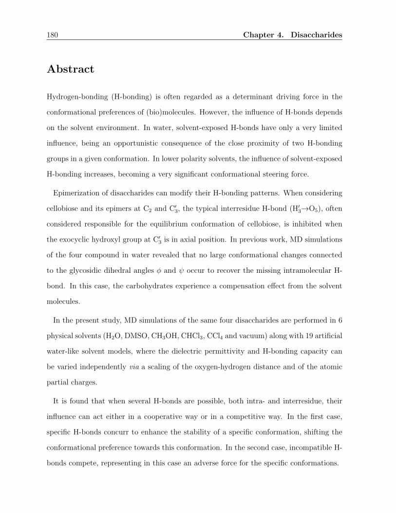
180 Chapter 4. Disaccharides
Abstract
Hydrogen-bonding (H-bonding) is often regarded as a determinant driving force in the
conformational preferences of (bio)molecules. However, the influence of H-bonds depends
on the solvent environment. In water, solvent-exposed H-bonds have only a very limited
influence, being an opportunistic consequence of the close proximity of two H-bonding
groups in a given conformation. In lower polarity solvents, the influence of solvent-exposed
H-bonding increases, becoming a very significant conformational steering force.
Epimerization of disaccharides can modify their H-bonding patterns. When considering
cellobiose and its epimers at C2 and C′3, the typical interresidue H-bond (H′3→O5), often
considered responsible for the equilibrium conformation of cellobiose, is inhibited when
the exocyclic hydroxyl group at C′3 is in axial position. In previous work, MD simulations
of the four compound in water revealed that no large conformational changes connected
to the glycosidic dihedral angles φ and ψ occur to recover the missing intramolecular H-
bond. In this case, the carbohydrates experience a compensation effect from the solvent
molecules.
In the present study, MD simulations of the same four disaccharides are performed in 6
physical solvents (H2O, DMSO, CH3OH, CHCl3, CCl4 and vacuum) along with 19 artificial
water-like solvent models, where the dielectric permittivity and H-bonding capacity can
be varied independently via a scaling of the oxygen-hydrogen distance and of the atomic
partial charges.
It is found that when several H-bonds are possible, both intra- and interresidue, their
influence can act either in a cooperative way or in a competitive way. In the first case,
specific H-bonds concurr to enhance the stability of a specific conformation, shifting the
conformational preference towards this conformation. In the second case, incompatible H-
bonds compete, representing in this case an adverse force for the specific conformations.

4.1. Introduction 181
4.1 Introduction
In the conformational analysis of (bio)molecules, different qualitative or semi-quantitative
effects are commonly invoked to rationalize the lower free energy of the experimentally
dominant state(s) relative to alternative ones. Effects or classes of interactions stabiliz-
ing a specific conformation (e.g. native for a macromolecule or bound for a host-guest
complex) relative to less structured ones (e.g. unfolded or unbound) are termed driving
forces (controlling affinity), while those stabilizing one of the structured states relative to
alternative ones (e.g. alternative folds or binding modes) have been termed132 steering
forces (controlling selectivity). In this kind of analysis, many different types of effects can
be included, such as steric, stereoelectronic, electrostatic (e.g. hydrogen bonding) and
hydrophobic effects294–301.
Hydrogen bonding (H-bonding) is often considered to be a determinant driving force in
the conformational preferences of (bio)molecules. Indeed, early predictions concerning the
native state of proteins126 and nucleic acids127 were based on the consideration of optimal
H-bonding patterns. However, the influence of H-bonding cannot be discussed without
taking into account of the solute environment, i.e. the effect of the solvent. The importance
of H-bond formation for the conformational affinity or selectivity depends on the degree of
exposure of both the separated H-bonding partners (in one conformation) and the formed
H-bond (in the other conformation) to the solvent. In particular, the importance of H-
bond formation is different when two solvated H-bonding partners associate to form a
buried or a solvent-exposed H-bond. When forming a buried H-bond, the electrostatic
gain upon H-bond formation should be compared with the initial desolvation penalty of
the H-bonding partners. When forming a solvent-exposed H-bond, the formed H-bond
can be subject to H-bonding competition by the solvent molecules and the interaction
screened by the solvent dielectric response.

182 Chapter 4. Disaccharides
In the context of carbohydrates in solution, the influence of solvent-exposed H-bonding
on the stability of specific conformations is particularly relevant. In an aqueous environ-
ment, solvent-exposed H-bonds in carbohydrates can be considered to represent a minor
(possibly negligible or even, in some cases, adverse) conformational driving as well as
steering force (see Ref.132 and Chapter 3). They should be viewed as an opportunistic
consequence of the close proximity of two H-bonding groups in a given conformation, and
not as a factor contributing to the stability of this conformation132,171. However, as the po-
larity of the solvent is decreased, solvent-exposed intramolecular H-bonding progressively
evolves from a negligible (possibly adverse) to a very significant (favorable) conformational
driving force.
This view is compatible with the experimental observation that the hydroxymethyl rot-
amers of glucose and galactose permitting the formation of a solvent-exposed H-bond
between this group and the hydroxyl group at C4 are not favored but, in the opposite,
least populated in water184,185,191. The evolution of the rotameric preferences in lower
polarity solvents was investigated in Chapter 3 As the solvent polarity is decreased, the
populations of the conformers compatible with the formation of the intramolecular H-bond
was found to increase significantly.
Evaluations concerning the importance of H-bonding are comparatively easy when con-
sidering a simple system such as a monosaccharide. On the other hand, when considering
more complex systems such as oligosaccharides or polysaccharides, the number of factors
involved in the stability of specific conformations can increase drastically. Additionally,
this kind of molecules shows secondary-structure patterns analogous to the ones found
in proteins, although often local and transient. For this reason, the corresponding con-
formations are commonly classified based on similar schemes302–305, e.g. Ramachandran
maps for the glycosidic linkages and secondary-structure elements such as regular helices).
Note, however, that polysaccharides evidence a more pronounced constitutional variety

4.1. Introduction 183
and conformational flexibility compared to proteins.
Disaccharides are the simplest carbohydrates involving all types of degrees of freedom
present in longer chains, while still involving a limited number of effects. These molecules
are thus particularly appealing for theoretical investigations. Numerous studies concern-
ing the conformational preferences of disaccharides can be found in the literature, both
experimental306–314 and theoretical132,169,315–321. Many of these invoked solvent-exposed
H-bond formation to rationalize specific conformational preferences of aqueous disacchar-
ides302,306,322–324. In contrast, a smaller number of studies132,171,245 (see also Chapter 3)
suggested that, in the opposite, solvent-exposed H-bonding should not be considered as a
major factor influencing those preferences in an aqueous environment.
The starting point of the present study is the article of Wang et al.132 concerning the
conformational preferences of cellobiose and its C2 and C′3 epimers in aqueous solution.
The four epimers considered present a different stereochemistry for the potentially H-
bonding groups neighboring the glycosidic linkage. The absence of significant differences
in the distributions of the glycosidic dihedral angles φ and ψ supported the suggestion of
a negligible influence of solvent-exposed H-bonding on the conformational properties of
these four compounds in water. The present study revisits this system, now considering
the influence of the solvent polarity on the conformational properties. The same four
epimers are simulated here using explicit-solvent molecular dynamics (MD) simulations
in physical solvents of various polarities, as well as in the artificial solvents developed
in Chapter 2. These were previously employed (Chapter 3) to disentangle the influence
of the solvent dielectric permittivity and H-bonding capacity, while preserving water-like
dispersive interactions as well as molecular size and shape, on the rotameric equilibrium
of the hydroxymethyl group in glucose and galactose.
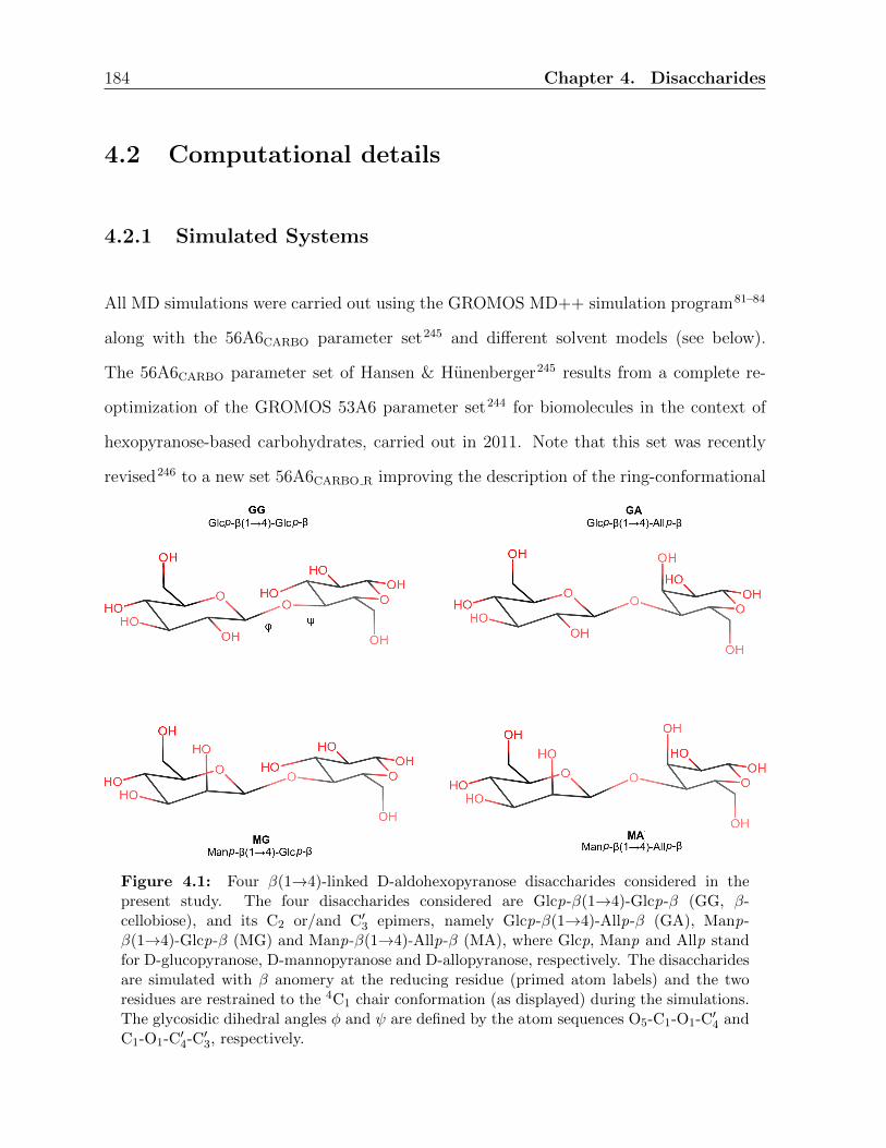
184 Chapter 4. Disaccharides
4.2 Computational details
4.2.1 Simulated Systems
All MD simulations were carried out using the GROMOS MD++ simulation program81–84
along with the 56A6CARBO parameter set245 and different solvent models (see below).
The 56A6CARBO parameter set of Hansen & Hunenberger245 results from a complete re-
optimization of the GROMOS 53A6 parameter set244 for biomolecules in the context of
hexopyranose-based carbohydrates, carried out in 2011. Note that this set was recently
revised246 to a new set 56A6CARBO R improving the description of the ring-conformational
Figure 4.1: Four β(1→4)-linked D-aldohexopyranose disaccharides considered in thepresent study. The four disaccharides considered are Glcp-β(1→4)-Glcp-β (GG, β-cellobiose), and its C2 or/and C′3 epimers, namely Glcp-β(1→4)-Allp-β (GA), Manp-β(1→4)-Glcp-β (MG) and Manp-β(1→4)-Allp-β (MA), where Glcp, Manp and Allp standfor D-glucopyranose, D-mannopyranose and D-allopyranose, respectively. The disaccharidesare simulated with β anomery at the reducing residue (primed atom labels) and the tworesidues are restrained to the 4C1 chair conformation (as displayed) during the simulations.The glycosidic dihedral angles φ and ψ are defined by the atom sequences O5-C1-O1-C′4 andC1-O1-C′4-C′3, respectively.
4.2. Computational details 185
properties for residues within chains. However, this change would not be expected to affect
significantly the results presented here as dihedral-angle restraints are applied to prevent
ring inversions (see Section 4.2.2).
The simulations involved cubic computational boxes containing one solute molecule and
Ns solvent molecules. The solutes considered are the four β(1→4)-linked D-aldohexo-
pyranose disaccharides with β anomery at the reducing residue illustrated in Figure
4.1, namely Glcp-β(1→4)-Glcp-β (GG, β-cellobiose), Glcp-β(1→4)-Allp-β (GA), Manp-
β(1→4)-Glcp-β (MG) and Manp-β(1→4)-Allp-β (MA), where Glcp, Manp and Allp stand
for D-glucopyranose, D-mannopyranose and D-allopyranose, respectively. Considering the
most stable 4C1 chair conformation of the two residues and labeling the atoms of the re-
ducing residue with a prime, the four disaccharides present equatorial orientations of the
hydroxyl groups at C3, C4, C′1 and C′2 as well as of the hydroxymethyl groups at C5 and C′5,
along with different orientations of the hydroxyl groups at C2 and C′3, namely equatorial-
equatorial (GG), equatorial-axial (GA), axial-equatorial (MG) or axial-axial (MA). Note
that the parameters of the four disaccharides in the 56A6CARBO force field differ exclusively
in terms of the sign of the reference improper-dihedral angle controlling the stereochem-
istry at carbon atoms C2 and C′3, i.e., the bond, bond-angle, torsional and non-bonded
interaction parameters of the four compounds are otherwise rigorously identical. The four
solutes were simulated in various physical and artificial solvents.
For the physical solvents, the models considered are the SPC water (H2O) model of
Berendsen et al.136 (Ns = 2081), the dimethyl-sulfoxide (DMSO) model of Geerke et al.149
(Ns = 543), the methanol (CH3OH) model of Walser et al.252 (Ns = 952), the chloroform
(CHCl3) model of Tironi and van Gunsteren254 (Ns = 479), and the carbon-tetrachloride
(CCl4) model of Tironi et al.256 (Ns = 398). The indicated values of Ns result in cubic
computational boxes of about 4.0 nm edge length in all cases. The four solutes were also
simulated in vacuum (VAC), using stochastic dynamics (SD)100,101 instead of MD in this

186 Chapter 4. Disaccharides
Sol
vent
ρ[k
g·m−
3]
µ[D
]ε
δHE
xp.
Ref
.Sim
.R
ef.
Exp.
Ref
.Sim
.R
ef.
Exp.
Ref
.Sim
.R
ef.
Exp.
Ref
.H
2O
997
147
973
138
1.85
249
2.27
136
78.5
138
66.0
138
42.3
250
DM
SO
1095
251
1096
149
3.96
166
5.25
149
46.0
251
38.0
149
10.2
250
CH
3O
H79
1251
785
252
1.70
253
2.29
252
32.6
253
19.8
252
22.3
250
CH
Cl 3
1489
251
1520
254
4.81
251
2.30
255
4.8
253
2.4
254
5.7
250
CC
l 415
95253
1601
256
0.00
0.00
2.2
166
1.0
256
-V
AC
--
--
1.0
1.0
-
Table
4.1:
Exp
erim
enta
lan
dsi
mu
late
dp
rop
erti
esof
the
physi
cal
solv
ents
con
sid
ered
inth
ep
rese
nt
stud
yat
298.
15K
and
1b
ar.
Th
equ
anti
ties
rep
orte
dar
eth
ed
ensi
tyρ,
the
gas-
ph
ase
mol
ecu
lar
dip
ole
mom
entµ
,th
est
atic
rela
tive
die
lect
ric
per
mit
tivit
yε,
and
the
Han
sen
par
amet
er250δH
asa
mea
sure
ofth
eH
-bon
din
gp
rop
ensi
ty.

4.2. Computational details 187
specific case. For convenience, basic properties characterizing the polarity of the five
physical solvents, either experimental or based on previous simulations with the indicated
models, are summarized in Table 4.1.
The artificial solvents considered are a subset of the tunable solvents introduced in
Chapter 2 and used in Chapter 3 to be employed under constant-volume (NVT) condi-
tions. These water-derived models were generated starting from the SPC water model of
Berendsen et al.136, by changing systematically the oxygen-hydrogen bond length (scaling
factor sb) and the atomic partial charges (scaling factor sq), without any change in the
Lennard-Jones interaction parameters. The scaling factors sb and sq were both varied
systematically by increments of 0.1 in the range 0.1 to 1.5, leading to the definition of
195 water-derived models (35 extreme combinations of sb and sq were not retained as
the resulting models could only be simulated using very small timesteps). These models
have different dielectric permittivities and H-bonding capacities, but identical dispersive
interactions as well as molecular shape and size. They are labeled W sbsq according to the
values of the two scaling factors, so that in particular W 1.01.0 is the SPC water model. The
main thermodynamic, dynamic, dielectric and H-bonding properties of these 195 solvents
as calculated based on pure-liquid simulations, can be found in Suppl. Mat. Table 2.S.1
of Chapter 2. Their dielectric permittivities ε and H-bonding capacities nH , the latter
value being defined as the average number of H-bonds per molecule in the pure liquid, are
illustrated graphically in Figure 4.2. In this set of 195 solvents, a subset of 19 is considered
here, corresponding to four series SHp , Shp , SPh , and Sph. These series permit to investigate
specifically the effect of the following trends: (i) in series SHp , the progressive decrease of
the permittivity (p subscript) at water-like H-bonding capacity (H superscript); (ii) in
series Shp , the progressive decrease of the permittivity (p subscript) at lower H-bonding
capacity (h superscript); (iii) in series SPh , the progressive decrease of the H-bonding
capacity (h subscript) at water-like permittivity (P superscript); (iv) in series Sph, the

188 Chapter 4. Disaccharides
progressive decrease of the H-bonding capacity (h subscript) at lower permittivity (p su-
perscript). The properties of the 19 artificial solvents along with the definition of the four
series are summarized in Table 4.2. These models and the corresponding series are also
shown graphically in Figure 4.2. Note that the SPC water model W 1.01.0 belongs to both
series SHp and SPh . For the artificial solvents, the number of solvent molecules Ns in the
computational box was always set to 2081 for a cubic box of edge length 4.0 nm.
Series Solvent sb sq ε nH
SHp
W 0.81.4 0.8 1.4 115 3.4
W 0.91.2 0.9 1.2 89 3.5
W 1.01.0 (SPC) 1.0 1.0 64 3.4W 1.5
0.5 1.5 0.5 25 3.4
Shp
W 0.51.4 0.5 1.4 36 1.7
W 0.80.9 0.8 0.9 33 2.0
W 0.70.6 0.7 0.6 7 1.5
W 0.50.3 0.5 0.3 1 1.4
SPh
W 1.10.9 1.1 0.9 56 3.6
W 1.01.0 (SPC) 1.0 1.0 64 3.4W 0.8
1.1 0.8 1.1 64 2.5W 0.7
1.2 0.7 1.2 65 2.2W 0.6
1.4 0.6 1.4 76 2.0W 0.5
1.5 0.5 1.5 49 1.7
Sph
W 1.50.4 1.5 0.4 14 2.6
W 1.20.5 1.2 0.5 15 2.2
W 1.10.5 1.1 0.5 13 1.9
W 0.80.7 0.8 0.7 15 1.7
W 0.60.9 0.6 0.9 14 1.6
W 0.41.3 0.4 1.3 12 1.5
Table 4.2: Definition and simulated properties of the 19 artificial solvent models consideredin the present study at 298.15 K and 968 kg·m−3. The reported quantities are the scalingfactors sb and sq applied to the oxygen-hydrogen bond length and to the atomic partialcharges, respectively, relative to the SPC water model136, the static relative dielectric per-mittivity ε of the liquid, and the average number nH of H-bonds per molecule in the liquidas a measure of its H-bonding capacity. The models are grouped into four series as describedin section 2.1. Note that the SPC water model W 1.0
1.0 belongs to both series SHp and SPh .These 19 models are a subset of the 195 models developed in Chapter 2, (see also Chapter 3)their main thermodynamic, dynamic, dielectric and H-bonding properties being reported inSuppl. Mat. Table 2.S.1 of Chapter 2.

4.2. Computational details 189
Figure 4.2: Simulated properties of the 195 artificial solvent models developed in Chapter 2at 298.15 K and 968 kg·m−3. The static relative dielectric permittivity ε of the liquid (a) andthe average number nH of H-bonds per molecule in the liquid (b) are shown as a function ofthe scaling factors sb and sq applied to the oxygen-hydrogen bond length and to the atomicpartial charges, respectively, relative to the SPC water model136. The squares identify thesubset of 19 models considered in the present study, colored according to the four series(SHp , Shp , SPh , and Sph; Table 4.2). The SPC model W 1.0
1.0 is shown in violet and belongs to
both SHp and SPh . The areas in black and gray correspond to models that are either notin the set (30 sb and sq combinations were disregarded as the corresponding models couldonly be simulated with very short timesteps) or not liquid (glassy state), respectively, at thetemperature and density considered. The main thermodynamic, dynamic, dielectric andH-bonding properties of the 195 models are reported numerically in Suppl. Mat. Table2.S.1 of Chapter 2.
4.2.2 Simulations
The simulations performed include explicit-solvent MD simulations of the four solutes
(GG, GA, MG, MA) in the two different sets of solvents (5 physical and 19 artificial),
where the sampling along the dihedral angles φ and ψ was enhanced by the local-elevation
umbrella-sampling (LEUS) approach14,90,105, along with plain SD simulations100,101 of the
four compounds in vacuum. Additional plain MD simulations involving restraints to spe-
cific conformational regions were also performed in the physical solvents.
The MD simulations were performed under periodic boundary conditions based on cubic
computational boxes containing one solute and Ns solvent molecules (values of Ns given in

190 Chapter 4. Disaccharides
Section 4.2.1). For the physical solvents, the simulations were carried out in the isothermal-
isobaric (NPT) ensemble at 298.15 K and 1 bar. For the artificial solvents, the simulations
were carried out in the canonical (NVT) ensemble at 298.15 K and an effective solvent
density of 998.7 kg·m−3. Here, the effective solvent density is estimated as V −1M(Ns+Ns),
where V is the box volume, M the molecular mass of water, and Ns an effective number
of water molecules accounting for the solute volume (set here to Ns = 24).
The simulations involving the artificial solvent models must be carried out under NVT
conditions because the Lennard-Jones interaction parameters of these models were not
adjusted to reproduce the equilibrium density of water at 298.15 K and 1 bar. Accordingly,
under NVT conditions at 298.15 K and 968 kg·m−3, they are characterized by equilibrium
pressures that range from -0.6 to 8.9 kbar for the 19 models considered here (see Suppl.
Mat. Table 2.S.1 of Chapter 2). However, incorrect pressures are expected to have only
a limited influence on the glycosidic dihedral-angle rotation in disaccharides, as was the
case for the rotameric equilibrium of the hydroxymethyl group in monosaccharides (see
Section 2.2.2 in Chapter 3).
In both the NPT and NVT simulations, the temperature was maintained close to its
reference value of 298.15 K by weakly coupling115 solute and solvent degrees of freedom
jointly (to avoid solute damping264) to an external bath using a relaxation time of 0.1
ps. In the NPT simulations, the pressure was also maintained close to its reference value
of 1 bar by weakly coupling115 the atomic coordinates and the box dimensions (isotropic
coordinate scaling, group-based virial) to an external bath using a relaxation time of 0.5 ps
and an isothermal compressibility of 4.575·10−4 kJ−1·mol·nm3 as appropriate for aqueous
biomolecular systems101. The compressibility was not adjusted for the different solvents,
because it is combined with the arbitrary choice of a pressure relaxation time and does not
affect the average thermodynamic properties of the system. The center of mass translation
was removed every timestep.

4.2. Computational details 191
The leap-frog algorithm103 was used to integrate Newtonas equations of motion with a
timestep of 2 fs. Solute bond-length constraints as well as the full rigidity of the solvent
molecules were enforced by application of the SHAKE procedure53 with a relative geo-
metric tolerance of 10−4. The non-bonded interactions were calculated using a twin-range
scheme69, with short- and long-range cutoff distances set to 0.8 and 1.4 nm, respectively,
and an update frequency of 5 timesteps for the short-range pairlist and intermediate-range
interactions. A reaction-field correction60,65 was applied to account for the mean effect of
electrostatic interactions beyond the long-range cutoff distance, using the relative dielectric
permittivity appropriate for the solvent model considered (Tables 4.1 and 4.2).
The LEUS method14,90,105,132,171 was applied to enhance the sampling around the di-
hedral angles φ and ψ (O5-C1-O1-C′4 and C1-O1-C′4-C′3, see Figure 4.1) characterizing the
conformation of the glycosidic linkage, which can present long-timescale transitions in
unbiased simulations (on the order of171 10 ns up to a few µs). The LEUS calculations
involved two steps: (i) a local elevation (LE) build-up phase90 of duration tLE = 50 ns,
to progressively optimize a two-dimensional memory-based biasing potential in the space
defined by φ and ψ; (ii) an umbrella sampling (US) phase105 of duration tUS = 60 ns, us-
ing this preoptimized (now time-independent) biasing potential to enhance the sampling.
The biasing potential was represented by means of a grid of 32×32 truncated-polynomial
basis functions270 with a spacing of 11.25 along both φ and ψ. The polynomial widths
were set equal to the grid spacing. The LE build-up phase relied on a fixed force-constant
increment per visit set to kLE = 10−4 kJ·mol−1.
Five additional LEUS simulations were performed for the GG disaccharide in each of
the five physical solvents in order to check the convergence of the method with respect to
the memory build-up time. These involved biasing potentials obtained from LE build-up
phases of different durations (tLE = 0, 10, 20, 30 or 40 ns) along with a sampling phase
of normal duration tUS = 60 ns. All the other parameters were the same as for the main
192 Chapter 4. Disaccharides
simulations. Together with the main simulation involving tLE = 50 ns, the six simulations
involving different tLE are labelled tLE-LEUS. The convergence of the method with respect
to the US sampling time was also assessed, by truncating the US phase of the simulation
with tLE = 50 ns after different durations (tUS = 10, 20, 30, 40, 50, 60 ns). These six
simulations involving different tUS are labelled tUS-LEUS
Four additional plain MD simulations (no LEUS) were also performed for each of the
four disaccharides in each of the five physical solvents, involving restraints confining the
φ and ψ dihedral angles to specific ranges. These ranges correspond to the areas labelled
B, C1, C2 and C3 in the Ramachandran map of Figure 4.3 (further discussed in Section
4.2.3). The restraint involved flat-bottom half-harmonic potentials applied starting from
the edges of the corresponding regions with a force constant kres = 0.1 kJ·mol−1·deg−2.
These simulations were carried out for a duration tMD = 100 ns. All the other parameters
were the same as for the main simulations. These simulations are labelled MD-X, where
X refers to the specific range (B, C1, C2 or C3) considered.
The plain SD simulations (no LEUS) in vacuum were performed by integrating the
Langevin equation of motion100,101. They relied on a reference temperature of 298.15 K
and a friction coefficient of 91 ps−1. The choice of the latter value, appropriate for water100,
has no effect on the thermodynamic properties of the system. The SD simulations were
carried out for a duration tSD = 1 µs.
Because ring conformational transitions (chair inversion from 4C1 to 1C4 or conversion
to boat conformations) occur experimentally on the 0.05-1 µs timescale269,325,326, and al-
though the corresponding alternative conformations contribute negligibly to the conform-
ational ensembles of most aqueous aldohexopyranoses under ambient conditions261, their
occasional occurrence may compromise the statistical accuracy of the simulated results on
the timescale of a few tens of nanoseconds. For this reason, a restraining of the improper

4.2. Computational details 193
dihedral angles α1, α2 and α3 (defined according to Pickett and Strauss271 as C4-O5-C2-
C1, O5-C2-C4-C3, and C2-C4-O5-C5 decreased by 180) was applied in all simulations to
maintain the two rings in a 4C1 conformation. The restraints relied on reference values
of −35 for α1, α2 and α3, along with a force constant of 165.15 kJ·mol−1. Additional
simulations investigating the possible influence of the ring conformation on the glycosidic
linkage preferences are reported and discussed in Appendix 4.A.
For the MD+LEUS, the plain MD and the SD simulations, the initial structure of the
solute was in the 4C1 chair conformation for both residues, and the glycosidic linkage was
set in an initial conformation with φ = 300 and ψ = 60. After filling the computational
box with Ns molecules of the solvent considered, the equilibration consisted of a steepest-
descent energy minimization, followed by a 0.5 ps thermalization MD (NVT, progressively
increased temperature) and by a 1 ns plain MD simulation (NVT for the artificial solvents,
NPT for the physical solvents, constant temperature). From this point, configurations
(along with the value of the biasing potential in the US sampling phases of the LEUS
simulations) were written to file every 0.5 ps for subsequent analysis.
4.2.3 Analysis
The analysis of the simulations was performed in terms of: (i) free-energy maps G(φ, ψ)
in the space of the glycosidic dihedral angles φ and ψ, along with corresponding relative
free energies GX of different states (conformational regions) and GX of the associated
minima at locations φX and ψX ; (ii) populations PX of the different states; (iii) average
number ni of intramolecular H-bonds; (iv) average number ns of solute-solvent H-bonds;
(v) relative populations p of the canonical rotamers (gg, gt, tg) of the two hydroxymethyl
groups (dihedral angles ω and ω′) and of the three staggered conformers (g+, t, g−) of the
exocyclic dihedral angle χ2 and χ′3. For the MD+LEUS simulations, all the thermodynamic

194 Chapter 4. Disaccharides
and structural quantities analyzed were calculated based on the configurations generated
during the US sampling phase, with a reweighting factor depending on the value of the
biasing potential associated with each configuration, as detailed elsewhere14.
The free-energy maps G(φ, ψ) in the space of the glycosidic dihedral angles φ and ψ
were calculated using a grid spacing ∆φ = 2 and ∆ψ = 2, and anchored (G = 0 kJ
mol−1) at their global minimum. In the tLE-LEUS and tUS-LEUS simulations, the value
of G at grid points that were never visited during a simulation, which is formally infinite,
was arbitrarily set to the maximal value Gmax of G over all grid points that were visited
at least once. For all other simulations, this value was set to Gmax = 50 kJ mol−1.
For the ease of discussion, the free-energy maps were partitioned into three distinct
conformational regions (A, B, and C) as illustrated in Figure 4.3, using cutoff values
similar to those employed in Ref.171 (although a different labelling is used here). The
region C was further partitioned into three subregions (C1, C2 and C3), using cutoff values
chosen by visual inspection of the free-energy maps. Whenever a region encompassed a
local minimum, the location of this minimum was determined by interpolation based on
the nearest-neighbor grid points. Minima occurred in regions B, C1, C2 or/and C3, but
never in region A. The location and free-energy of a minimum occurring in region X are
noted (φX , ψX) and GX , respectively. Alternatively, the relative free energies of the states
were calculated based on the corresponding integrated populations. Only states B, C1,
C2 or/and C3 were populated, never A. The relative free energy of state X is noted GX ,
anchored to zero for the most populated state. Corresponding relative populations PX are
also reported, expressed in percent.
The occurrence of intramolecular H-bonds was analyzed considering all hydroxyl groups
as potential H-bond donors and all hydroxyl or ring oxygen atoms as potential acceptors.
An intramolecular H-bond is assumed to be present when the distance between the hy-

4.2. Computational details 195
Figure 4.3: Definition of the five conformational regions in the Ramachandran (φ,ψ) mapsof the disaccharides. The regions A, B, and C are defined by cutoff values of 120 and 240
for φ and ψ, respectively, according to Ref.171 (with a different nomenclature: regions A,B and C correspond to the regions labelled B, D and A+C, respectively, in Ref.171). Theregion C is further partitioned in three subregions (C1, C2, and C3), with cutoff values of120, 230 and 340 for φ. Note that region C3 encompasses areas at the left and right of themap by periodicity. The regions are displayed superimposed to an illustrative free energymap corresponding to GG in water (first panel in Figure 4.6). Schematic representationsof the ring orientations corresponding to the five regions are also shown. The darker shadeindicates the α-face of the ring, the line pairs the hydroxymethyl groups, the single lines thehydroxyl groups at C2 or C′3 and the black circles the ring oxygen atoms.
196 Chapter 4. Disaccharides
drogen and acceptor atoms is below 0.25 nm, and the angle between the donor, hydrogen
and acceptor atoms is above 100. The use of a somewhat relaxed angular criterion170 (a
minimum angle of 135 is typically used instead101) is necessary to encompass H-bonds
between the vicinal hydroxyl groups in the ring and between the hydroxymethyl group
and the ring oxygen atom (see also Chapter 3).
The occurrence of solute-solvent H-bonds involving all the solute hydroxyl groups as well
as the ring oxygen atom was also analyzed, using the normal angular criterion (minimum
angle of 135). For the artificial solvent models involving a scaling of the oxygen-hydrogen
bond length (scaling factor sb 6= 1.0), the solute-solvent H-bond analysis of each trajectory
configuration was preceded by a rescaling of the solvent oxygen-hydrogen distances as
described in Chapter 2 and Chapter 3. This procedure involves a displacement of the
hydrogen atoms of each solvent molecule along the oxygen-hydrogen bond vector, while
keeping the oxygen position fixed, so that the value of 0.1 nm corresponding to the SPC
water model is recovered.
Relative populations p of the canonical rotamers (gg, gt, tg) of the two hydroxymethyl
groups (dihedral angles ω defined as C4-C5-C6-O6 and ω′ defined as C′4-C′5-C′6-O′6) and of
the three staggered conformers (g+, t, g−) of the exocyclic dihedral angles χ2 (C1-C2-O2-
H2) and χ′3 (C′2-C′3-O′3-H′3) were calculated from the probability distribution profiles around
the corresponding four dihedral angles. For the two hydroxymethyl dihedral angles, values
in the ranges [0; 120[, [120; 240[ and [240; 360[ define the relative populations of the
gg, gt and tg rotamers, respectively. For the two exocyclic hydroxyl dihedral angles the
corresponding ranges define the g+, t and g− rotamers.

4.3. Results 197
4.3 Results
4.3.1 Convergence assessment
Biased (i.e. non-reweighted) probability distributions PN(φ, ψ) in the space of the glyc-
osidic dihedral angles φ and ψ along with free-energy maps G(φ, ψ) obtained from the
tUS = 60 ns US phases of the six tLE-LEUS simulations involving different build-up times
tLE are displayed in Figure 4.4 for the disaccharide GG in the solvent CCl4. Similar res-
ults were obtained for the four other physical solvents considered (data not shown). These
maps permit to assess the convergence of the results as a function of the time tLE invested
into the LE build-up of the memory-based biasing potential prior to the US sampling
phase.
The comparison of the biased probability distributions PN for the six runs reveals a
large sampling enhancement upon increasing tLE from 0 ns to 30 or 40 ns. The effect
of increasing tLE further to 50 ns is comparatively more limited. The free-energy maps
calculated from the corresponding reweighted probability distributions show that all the
relevant minima are already revealed with tLE set to 10 ns. The maximal height above the
global minimum up to which the free-energy surface is explored increases systematically
with tLE, from about 30 to about 50 kJ·mol−1. The choice tLE = 50 ns retained in the
production simulations seems therefore to be adequate.
For tLE = 50 ns, a convergence assessment was also performed in terms of the US
sampling time tUS in the six tUS-LEUS simulations. The results are shown in Figure 4.5,
again for GG in CCl4. In this case, the sampling of the relevant region, particularly C,
is almost completely performed in the first 20 ns of the US phase. The maximal height
above the global minimum increases with tUS, from about 40 to about 50 kJ·mol−1. The
choice tUS = 60 ns retained in the production simulations was found sufficient.

198 Chapter 4. Disaccharides
Figure 4.4: [Next page] Convergence of the calculated biased probability distribution andfree-energy map as a function of the LE build-up time. The results are shown for thecompound GG (Figure 4.1) simulated in CCl4 at 1 bar and 298.15 K. They are based on thetUS = 60 ns US sampling phases of LEUS simulations relying on a biasing potential built upin LE phases of different durations tLE . The corresponding biased probability distributions(six panels on the left) and the free-energy maps (six panels on the right) in the space ofthe glycosidic dihedral angles φ and ψ are displayed. The free-energy maps are anchored toG = 0 kJ mol−1 at the location of their global minimum, and the value of G at grid pointsthat were never visited during the simulation is arbitrarily set (for each panel separately)to the maximal value Gmax of G over all grid points that were visited at least once.

4.3. Results 199
Figure 4.5: Convergence of the calculated biased probability distribution and free-energymap as a function of the US build-up time. The results are shown for the compound GG(Figure 4.1) simulated in CCl4 at 1 bar and 298.15 K. They are based on the tUS = 10, 20,30, 40, 50, 60 ns US sampling phases of LEUS simulations relying on a biasing potentialbuilt up in tLE = 50 ns LE phases. The corresponding biased probability distributions (sixpanels on the left) and the free-energy maps (six panels on the right) in the space of theglycosidic dihedral angles φ and ψ are displayed. The free-energy maps are anchored to G= 0 kJ mol−1 at the location of their global minimum, and the value of G at grid pointsthat were never visited during the simulation is arbitrarily set (for each panel separately)to the maximal value Gmax of G over all grid points that were visited at least once.

200 Chapter 4. Disaccharides
4.3.2 Conformational analysis in the physical solvents
Illustrative free-energy maps G(φ, ψ) for the four disaccharides considered obtained from
the LEUS simulations (tLE = 50 ns, tUS = 60 ns, after reweighting) in the physical
solvents with highest and lowest polarities, namely H2O and CCl4, are shown in Figure 4.6.
The other physical solvents represent intermediate situations between these two extremes
(data not shown). The maps obtained in CCl4 can also be compared with maps obtained
from 1 µs SD simulations in vacuum (see Suppl. Mat. Figure 4.S.1). In the absence
of LEUS sampling enhancement, the sampling in vacuum is less broad compared to the
LEUS simulations and the maximum height above the global minimum reached in these
simulations is about 30 kJ·mol−1. Besides that, the maps are very similar.
The relative populations PX of the different conformational regions X as defined in
Figure 4.3 and the corresponding relative free energies GX are displayed in Figure 4.7
for the entire series of physical solvents. The data can also be found numerically in
Suppl. Mat. Tables 4.S.1 and 4.S.2, also including the heights GX and the locations
(φX , ψX) of the minima. To facilitate the interpretation of the conformational regions in
terms of structures, illustrative schematic models of the disaccharides in the five regions
considered are also shown in Figure 4.3. Note that these sketches are only meant to give a
pictorial representation of the relative orientations of the two monosaccharide rings and of
the proximity of specific exocyclic groups, and not a precise description of the molecular
structure.
The two following subsections discuss in turn the conformational properties of the four
disaccharides in water, and the changes observed when considering the four other (less
polar) physical solvents.

4.3. Results 201
(a)
(b)
Figure
4.6:
Fre
e-en
ergy
map
sG
(φ,ψ
)in
the
spac
eof
the
glyco
sid
icd
ihed
ral
angl
esφ
an
dψ
for
the
fou
rd
isac
char
ides
con
sid
ered
(Fig
ure
4.1)
inH
2O
orC
Cl 4
at1
bar
and
298.
15
K.
Th
em
aps
are
bas
edon
the
60n
ssa
mpli
ng
ph
ases
ofth
eco
rres
pon
din
gL
EU
Ssi
mu
lati
on
sin
wat
er(H
2O
,fo
ur
pan
els
(a))
and
inca
rbon
-tet
rach
lori
de
(CC
l 4,
fou
rp
anel
s(b
)).
Th
em
aps
are
anch
ored
toG
=0
kJ
mol−
1at
the
loca
tion
ofth
eir
glob
alm
inim
um
,an
dth
eva
lue
ofG
atgr
idp
oints
that
wer
en
ever
vis
ited
du
rin
gth
esi
mu
lati
ons
isar
bit
rari
lyse
tto
Gmax
=50
kJ
mol−
1.
Th
em
aps
are
show
nin
theφ
,ψ-p
lan
eas
vie
wed
from
the
top
,alo
ng
wit
hla
tera
lp
roje
ctio
ns
inth
eφ
,G-
andψ
,G-p
lan
es.

202 Chapter 4. Disaccharides
Conformational analysis in water
Visual inspection of the two-dimensional free energy maps for the four disaccharides in
H2O (Figure 4.6, panels (a)) reveals the following main features.
As was observed in previous work on the glucose-based disaccharides132,171, large areas
of the maps remain unexplored because they correspond to configurations involving steric
clashes between the atoms of the two residues. All maps are characterized by a lowest
free-energy basin in region C, along with one alternative metastable state in region B.
The global minimum is located for all the disaccharides in region C1 at about (φC1 ,
ψC1)=(290±5, 111±5), see Table 4.S.2. These values are compatible with the available
experimental estimates for cellobiose (GG) in water as inferred from nuclear magnetic
resonance (NMR) data327, namely (272, 99), or in the crystal form as inferred from
X-ray crystallographic data306,322, namely (284, 108). They are also close to the values
found in a previous simulation study of the same disaccharides with the GROMOS 45A4
force field132 and with values typically found using other recent empirical force fields328.
The region C1 presents in all cases the largest population PC1 , about 98% for GG and MG
or about 93% for GA and MA, see Table 4.S.1.
Alternative low free-energy wells correspond to different φ (0-60 in region C3, 180-220
in region C2) or ψ (300-320 in region B) values. These alternative wells are associated with
populations of at most about 7%. One should distinguish between wells that correspond
to a local minimum and wells that can be seen as a broadening of the global minimum
in region C1 (without a separating free-energy barrier). The region B is associated with
marginal populations (at most 0.4%) and represents a local minimum at about 19-20
kJ·mol−1 for GG and MG or 27-28 kJ·mol−1 for GA and MA. The regions C2 and C3,
associated with small populations of about 1% or less for GG and MG or up to about
7% for GA and MA, represent broadenings of the global minimum at C1. They present

4.3. Results 203
free-energy values of 11-13 kJ·mol−1 except region C2 for GA and MA, with values around
4-5 kJ·mol−1.
These results confirm the observations made in Ref.132. The epimerization has only
a very limited influence on the Ramachandran free-energy map of the GG disaccharide.
More precisely, the epimerization at C2 has no visible effect (no difference between GG
and MG), while the epimerization at C′3 (difference from GG to GA) only broadens the
C1 basin in the direction of lower φ values (also slightly lower ψ), i.e. towards region C2.
Conformational analysis in the other physical solvents.
The effect of drastically decreasing the polarity of the solvent can be seen by comparing
the two-dimensional free energy maps of the four disaccharides in CCl4 (Figure 4.6, panels
(b)) with the maps in H2O (top panels). The progressive trends along the series of five
physical solvents of decreasing polarity can be followed in Figure 4.7 (numerical values in
Suppl. Mat. Tables 4.S.1 and 4.S.2).
As observed in the case of H2O, large areas of the maps remain unexplored in CCl4.
The conformational regions explored in the two solvents are similar. All maps are still
characterized by a lowest free-energy basin in region C, along with an alternative meta-
stable state in region B. Note that the area sampled in the latter region for GA and MA
is noticeably broader in CCl4 compared to H2O. The subregion C1 of C is still the most
populated, but its population may decrease to 60% and, in contrast to H2O, the subregions
C2 and C3 may become alternative metastable states (true local minima).
In the case of GA and MA, a local minimum appears in subregion C2, located at (φC2 ,
ψC2)=(232±5, 80±5) for GA and (194±5, 80±5) for MA. In the case of GA this
minimum becomes the most stable state (global minimum), with the one in C1 presenting
a slightly higher free-energy value of about 1 kJ·mol−1. The two minima are separated by

204 Chapter 4. Disaccharides
a barrier of about 2 kJ·mol−1. In the case of MA the global minimum remains in C1 and
becomes narrower, while the minimum in C2 is at 8 kJ·mol−1.
Along the series of physical solvents in order of decreasing polarity (Figure 4.7), the
region C2 for GA is associated with an increasing population, from 7% in H2O to 24% in
CCl4, with a simultaneous decrease in the population of C1, from 93% in H2O to 76% in
CCl4. The population of C3 remains below 0.6% in all cases. The region C2 for MA shows
populations that change little upon decreasing the polarity of the solvent, remaining below
7% for all the physical solvents considered, while the single overwhelmingly populated
state is the one in the region C1 (relative population above 90% in all cases). For this
disaccharide, a slight increase in the population of the region C3 can be noticed, associated
with a lowering of the free energy of that region (no formation of a real minimum can be
observed in this area).
In the case of GG and MG, a second minimum appears in C3. The minimum is located at
(φC3 , ψC3)=(54±5, 118±5) for GG and (6±5, 106±5) for MG. In the case of GG, this
local minimum is separated from the global minimum by a very high barrier of 25 kJ·mol−1
(relative to the global minimum) and it presents a free energy of about 6 kJ·mol−1. In
the case of MG, the second minimum is at 0.5 kJ·mol−1 and is separated from the global
minimum by a very low barrier of about 2 kJ·mol−1. In addition, MG presents a third
minimum, located in region C2 at about 10 kJ·mol−1, with a higher barrier of 20 kJ·mol−1
(relative to the global minimum). In contrast, for GG, the region C2 represent a broadening
of the global minimum (no local minimum).
Along the series of physical solvents in order of decreasing polarity (Figure 4.7), for GG,
the populations of the region C2 and C3 both increase slightly from about 0.5% in H2O to
about 4% in CCl4. The population of C1 remains above 92% in all solvents. For MG, the
region C3 is associated with an increasing population upon decreasing the polarity of the

4.3. Results 205
Figure 4.7: Populations and relative free energies of specific regions (Figure 4.3) in theRamachandran free-energy maps for the four disaccharides considered (Figure 4.1) alongthe series of pysical solvents at 298.15 K and 1 bar. For a subset of the six regions Xof the Ramachandran map, the populations PX (three panels on the left) and the relativefree energies GX (three panels on the right) are displayed along the solvent series. Thepopulations PX are calculated by integrating the reweighted probability distributions in thespace of the glycosidic dihedral angles φ and ψ over the selected regions. The correspondingfree energies are reported relative to the region with the lowest value (in general in theregion C1, for this reason omitted). The region A has zero population and is therefore alsoomitted. The data are based on the 60 ns sampling phases of the corresponding LEUSsimulations. The data points follow the series of physical solvents (Table 4.1) in order ofdecreasing polarity. The different panels (top to bottom) correspond to the different regions.The regions C1, C2, and C3 are considered for the populations, while the regions B, C2 andC3 are considered for the relative free energies. The data is reported numerically in Suppl.Mat. Tables 4.S.1 and 4.S.2. Full free-energy maps for H2O and CCl4 are displayed inFigure 4.6.

206 Chapter 4. Disaccharides
solvent, from 1% in H2O to about 40% in CHCl3 and CCl4. Accordingly, the population
of the region C1 decreases from 98% in H2O to 60% in CHCl3 and CCl4. The population
of the region C2 remains constant and very low, despite the formation of a third minimum
in that area.
As mentioned in Section 4.3.2, there is no dramatic differences between the four disac-
charides in water, in line with observations made in previous work on either the same or
similar disaccharides132,171. However, significant conformational changes occur in solvents
of lower polarity. These can be summarized as follows. When the hydroxyl group at C′3
is equatorial (GG and MG), a local minimum appears in the region C3. This minimum
represents a metastable state when the hydroxyl group at C2 is equatorial (GG), whereas
it becomes a stable state comparable with the global minimum when this the hydroxyl
group is axial (MG). When the hydroxyl group at C′3 is axial (GA and MA), a second
minimum appears in region C2. This minimum represents a metastable state when the
hydroxyl group at C2 is axial (MA), whereas it becomes a stable state comparable with
the global minimum when this hydroxyl group is equatorial (GA).
4.3.3 Hydrogen bonding analysis in the physical solvents
The analysis of the H-bonds was performed considering all hydroxyl groups as potential H-
bond donors and all hydroxyl or ring oxygen atoms as potential acceptors, and is reported
in terms of average number n between specific potentially H-bonding partners. Note that
when a single H-bond is considered, n can be viewed as a relative occurrence of the H-
bond. The numbers ni of intramolecular H-bonds and the number ns of H-bonds with the
solvent are considered separately. The intramolecular H-bonds analysis also distinguishes
between numbers nir of intraresidue (i.e. within the same ring) and nit of interresidue (i.e.
trans-glycosidic) H-bonds. The former are only significant when the angular criterion used

4.3. Results 207
to define the presence of an H-bond is relaxed170 (from 135 to 100, see Section 4.2.3).
In addition, for these intraresidue H-bonds, the flip-flop alternatives are also listed as an
indicator of the presence of either a clockwise or a counterclockwise (as viewed from the
β-side of the ring) H-bond network (pattern 4→3→2→1 or pattern 1→2→3→4).
The H-bond analysis is provided in full details in Suppl. Mat., graphically in Figures
4.S.2-4.S.4 and numerically in Table 4.S.3. For a further analysis of the H-bonding pat-
terns, additional plain MD simulations, labelled MD-X (see Section 4.2.2), were performed
restraining the φ and ψ dihedral angles in the four region of Figure 4.3 (B, C, C1, C2 or
C3). The data regarding the H-bonding in the specific regions of Ramachandran maps
refer to these simulations, unless otherwise specified. To facilitate the discussion, a subset
of all these results is presented synoptically in Figures 4.8-4.11, along with Table 4.3.
Figure 4.8 gives a summary of the H-bond analysis, showing graphically the total number
nit of interresidue H-bonds, the total number nir of intraresidue H-bonds and the total
number ns of H-bonds with the solvent. Figure 4.9 provides a more detailed analysis of the
interresidue H-bonds in the four regions of Ramachandran map, together with information
on the conformations of the four exocyclic dihedral angles compatible with these H-bonds.
A preliminary analysis revealed that six possible interresidue H-bonds can occur, namely
H′3→O5, O6↔O′3, O2↔O′6, H′6→O5, O6↔O′6 and O2↔O′3, the double arrow indicating
the possibility of two filp-flop alternatives. These H-bonds are compatible with different
possible conformations of the φ and ψ dihedral angles, and involve specific orientations of
the four exocyclic dihedral angles ω, ω′, χ2 and χ′3. To better understand this correlation,
disaccharide structures were generated varying systematically the φ and ψ dihedral angles
by increments of 10, and considering the three standard orientations (gg, gt, tg) of the
hydroxymethyl groups (dihedral angles ω and ω′) and of the hydroxyl groups at C2 and C′3
(dihedral angles χ2 and χ′3). Figure 4.10 shows the results of this analysis. Additionally,

208 Chapter 4. Disaccharides
the list of all possible interresidue H-bonds for the different regions of the Ramachandran
map is given in Table 4.3. Finally, the occurring interresidue H-bonds are also shown in
illustrative structures presented in Figures 4.11.
Hydrogen bonding analysis in water
Figure 4.8 shows the total number of H-bonds for the four disaccharides considered, dis-
tinguishing between H-bonds with the solvent (dark green), intraresidue H-bonds (orange)
and interresidue H-bonds (gray). A rectangle with a color code consistent with that in Fig-
ure 4.7 also identifies each disaccharide. The values for the simulations in H2O correspond
to the set of four bars on the left.
In water, the average total number of H-bonds is about 17.5 (GA, MA) or 18 (GG, MG)
for all the disaccharides considered. The disaccharides have several potentially H-bonding
sites, namely six hydroxyl and two hydroxymethyl groups (that can be both donors and
acceptors), plus two ring and one glycosidic oxygen atoms (only acceptors). On average,
each site participates in 1.5 H-bonds. However, the distribution of these 17.5 or 18 H-bonds
among the three categories is different for the different compounds. For GG and MG, one
has about 15 H-bonds with the solvent, 2 intraresidue H-bonds and 1 interresidue H-bond.
The epimerization at C2 does not affect this pattern. On the other hand, epimerization
at C′3 (GA and MA) leads to a slightly different balance in the distribution of H-bonds.
When being in an axial position (MA), the hydroxyl group at C′3 is more solvent exposed
and the number of H-bonds with the solvent increases to about 16. At the same time,
the number of intraresidue H-bonds is decreased to about 1.5, and that of interresidue
H-bonds becomes nearly zero.
As can be seen in Figure 4.10, the typical interresidue H-bond present in the dominant
conformations at equilibrium for GG and MG is H′3→O5. The epimerization at C′3 clearly

4.3. Results 209
Figure 4.8: Numbers of H-bonds for the four disaccharides considered in the physicalsolvents at 298.15 K and 1 bar. The results are based on the 60 ns sampling phase ofthe corresponding LEUS simulations. Each bar represents the total number n of H-bonds,with different colors distinguishing interresidue H-bonds, intraresidue H-bonds, and solute-solvent H-bonds. The different bars for each solvent refer to one of the four disaccharides(Figure 4.1), that are identified by a box with the same color code as in Figure 4.7. Thebars follow the series of the physical solvents (4.1) in order of decreasing polarity. The datais reported numerically in Suppl. Mat. Table 4.S.3
affects the feasibility of such a H-bond. The most relevant alternative to this H-bond for
GG and GA is H′2→O6, compatible with the conformations in the region C1. Note that this
H-bond is no longer feasible for MG and MA in this region, due to the epimerization at C′3.
As already observed in previous work on either the same or similar disaccharides132,171,
the intramolecular H-bonding partners are in a highly polar solvent (water), and their
interaction is screened by the solvent dielectric response as well as subject to H-bonding
competition by the solvent molecules. The lack of a specific intramolecular H-bond is

210 Chapter 4. Disaccharides
easily compensated for by the interaction of the potential H-bonding partners with the
solvent molecules. This compensation prevents large conformational changes that would
be necessary to recover the lost intramolecular H-bond in the case of GA and MA, as
shown in the free energy maps discussed in the previous sections.
Figure 4.9: Numbers of interresidue H-bonds and exocyclic rotamer populations for thefour disaccharides considered in the physical solvents at 298.15 K and 1 bar. The resultsare based on plain MD simulations restrained to four regions (B, C1, C2 or C3) in the spaceof the glycosidic dihedral angles φ and ψ (Figure 4.3). The graphs on the left show thetotal numbers ni of interresidue H-bonds. The colors refer to the four disaccharides (GG,MG, GA and MA). The graphs on the right show the relative populations p (in percent)of three canonical rotamers (gg, gt, tg) of the two hydroxymethyl groups (dihedral anglesω and ω′) and of the three staggered conformers (g+, t, g−) of the exocyclic dihedral angleχ2 and χ′3 considering the solvents H2O and CCl4 only. The bars correspond to the relativepopulations of ω (1), ω′ (2), χ2 (3) and χ′3 (4) and the colors refers to the three possibleconformations of the dihedral angles (gg or g+, gt or t and tg or g−).
4.3. Results 211
Hydrogen bonding analysis in the other physical solvents
The effect of a decrease in the polarity of the solvent on the H-bonding pattern can be
see in Figure 4.8. An increase in the number of intramolecular H-bonds compensates for
the lower H-bonding propensity of the solvent. In CHCl3 and CCl4 the average number
of H-bonds with the solvent decreases to values close to zero and the average number of
intraresidue H-bonds increases to about 7 (GG), 6 (MG) or 4.5 (GA, MA). Note that the
average number of H-bonds with DMSO is lower than the one with CH3OH in spite of the
comparable dielectric permittivities of these two solvents (Table 4.1), because DMSO is
only an H-bond acceptor whereas CH3OH is both a donor and an acceptor
Differences between the four disaccharides considered in terms of intramolecular H-
bonding become pronounced in low polarity solvents. In CHCl3 and CCl4, GG shows
the highest number of both intraresidue (about 5) and interresidue (about 2) H-bonds.
The epimerization at C2 affects the interresidue H-bond formation, lowering the average
number to 1 for MG. The effect of the epimerization at C′3 is even more pronounced,
interfering with both types of intramolecular H-bonds. For both GA and MA the total
number of intraresidue H-bonds is about 4.5. In addition, the double epimerization in MA
also inhibits almost completely the formation of interresidue H-bonds.
The conformational changes described in the Section 4.3.2 upon decreasing the solvent
polarity can be explained by looking at Figure 4.10 and Table 4.3. This figure displays the
areas where each of the six possible interresidue H-bonds are possible for the four different
disaccharides. This permit to assess the compatibility between stable (or metastable)
states and the formation of normal (or alternative) H-bonds. The following patterns can be
identified. First, regions that are stabilized upon decreasing the solvent polarity (lowering
of the free energy and formation of a barrier to other states) are compatible with one
specific H-bond. This is the case for the minimum at C2 in MG and MA, compatible with

212 Chapter 4. Disaccharides
Comp. Conf.H-bonds
H’3→O5 O6↔O’3 O2↔O’6 H’6→O5 O6↔O’6 O2↔O’3
GG
B · g− · · t g−
g+· · · · g+
g−g+
t
C1 · · · t t · tg+· · g− g+ · · g+ · · t g+ · ·
C2 * · g− g+
g−·
C3 · g+g−· · g+
tg+
g−· · · · g+
g−g+
t
GA
B · · · t · g− · · t g−
g+· ·
C1 * * · g− g+ ·C2 * · g− g+ ·C3 · g+
g−· · g+
tg+
g−· ·
MG
B · g− g+
g−· · g− · · t g+
g−· ·
C1 · · · t t · tg+·
C2 · g− g−
g+· · g+ · ·
C3 * · g+g−· · g+
tg+
g−· · · · g+
g−g+
t
MA
B · · · t · g+g−· · t g+
g−· ·
C1 * *
C2 * · g− g−
g+·
C3 · g+g−· · t g+
g−· · · · g+
g−tg+
Table 4.3: Interresidue H-bonds compatible with specific areas of the Ramachandranmap given specific exocyclic group orientations for the four disaccharides considered. Thefeasibility of the six possible interresidue H-bonds (either of the two flip-flop possibilitiesconsidered together if possible) is indicated for the four region of the (φ,ψ) conformationalspace (Figure 4.3). For each possible H-bond, the implied conformation of the four exocyclicangles ω, ω′, χ2 and χ′3 is given. When a certain angle is not relevant for the formation ofa given H-bond, a dot is inserted. Two conformations for a pair of angles refer to the twoalternative flip-flop H-bonds, while two conformations for a single angle refer to two possiblealternative. A star indicates denoted a possibility that implies a larger deformation of the(φ,ψ) conformation relative to the values representative of the free-energy minimum in thespecific region.
an alternative O2↔O′6 H-bond. Second, regions that become comparable to the global
minimum (lowest free-energy) are compatible with two or more specific H-bonds. This is
the case for the minimum at C1 in GG, compatible with both H′3↔O5 and O2↔O′6, or the
minimum at C3 in MG, compatible with H′6→O5, O6↔O′6 and O2↔O′3. Third, regions
that show a lowering of the free energy but not the formation of an alternative minimum
are either compatible with two or more alternative H-bonds that are mutually excluding,
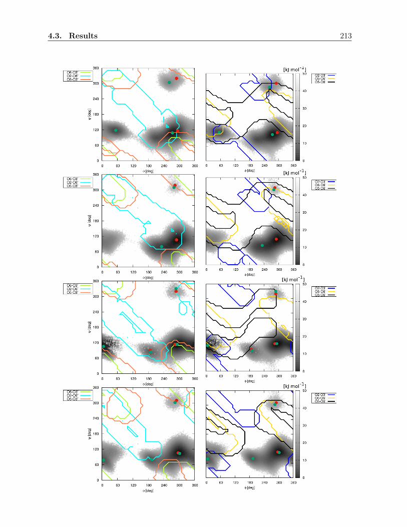
4.3. Results 213

214 Chapter 4. Disaccharides
Figure 4.10: [Previous page] Interresidue H-bonds compatible with specific configurationsof the glycosidic linkage for the four disaccharides considered. The contour of the areascompatible with a specific interresidue H-bond are displayed in the space of the glycosidicdihedral angles φ and ψ for the four disaccharides (Figure 4.1). They are superimposedto the free energy maps G(φ, ψ) obtained by LEUS simulations in CCl4 at 298.15 K and1 bar (see Figure4.6). The analysis is based on model conformations generated varyingsystematically the φ and ψ dihedral angles by increments of 10 and considering the threestandard orientations (gg, gt, tg) of the hydroxymethyl groups (dihedral angles ω and ω′)and the three standard orientations (g+, t, g−) of the hydroxyl groups at C2 and C′3 (dihedralangles χ2 and χ′3). The dots identify the local free-energy minima in H2O (red) and in CCl4(green). The different panels correspond to the four disaccharides, GG, GA, MG and MA(top to bottom). The six possible interresidue flip-flop H-bonds are illustrated, distringuish-ing between the H-bonds compatible with a conformation of the two rings with the oppositeorientation of the hydroxymethyl groups (left panels) and with the same orientation of thehydroxymethyl groups (right panels).
or partially compatible with different H-bonds given a slight shift of the φ and ψ dihedral
angles. This is the case for the region B of MG, compatible with either O6↔O′6 or O2↔O′6
(two H-bonds that cannot occur in the same conformation) or region C3 of MA, compatible
with H′6→O5, O6↔O′6 and O2↔O′3 (but with slightly different values of φ and ψ).
Based on this analysis, it can be suggested that with a system as complex as a disac-
charide, the effect of H-bonding in low-polarity solvents is either cooperative (two or more
H-bonds can strongly stabilize a conformational change, mutually enhancing their effect),
or stabilizing (one H-bond can stabilize a metastable state), or adverse (two or more H-
bonds compatible with slightly different conformations belonging to the same region but
that cannot be formed simultaneously within a single conformation can destabilize each
other and the specific conformational region they are both compatible with).
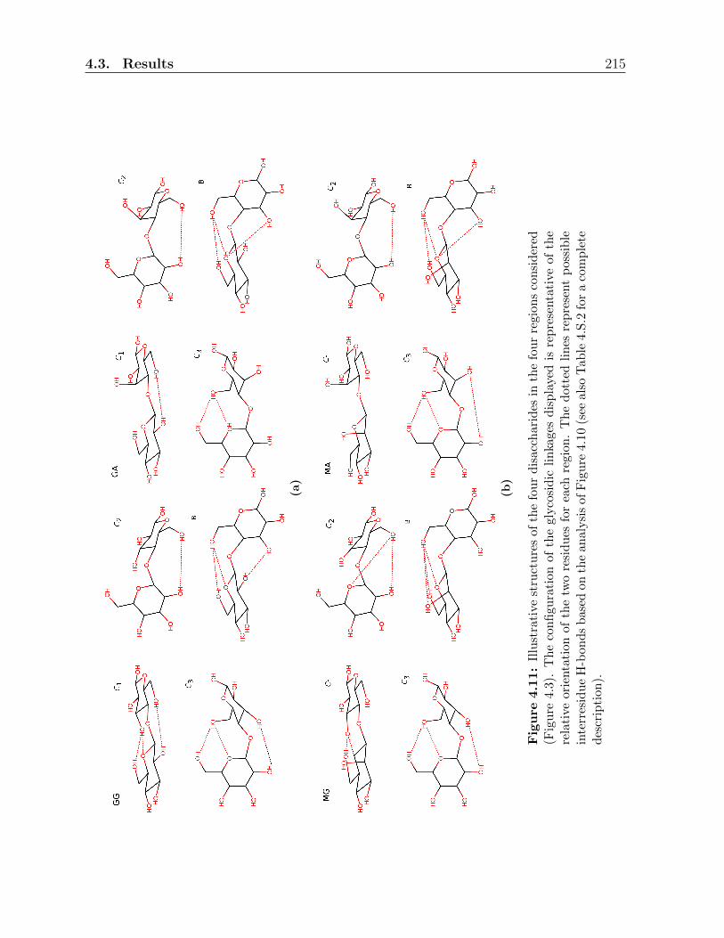
4.3. Results 215
(a)
(b)
Figure
4.11:
Illu
stra
tive
stru
ctu
res
ofth
efo
ur
dis
acch
arid
esin
the
fou
rre
gion
sco
nsi
der
ed(F
igu
re4.
3).
Th
eco
nfi
gura
tion
ofth
egl
yco
sid
icli
nka
ges
dis
pla
yed
isre
pre
senta
tive
of
the
rela
tive
orie
nta
tion
ofth
etw
ore
sid
ues
for
each
regi
on.
Th
ed
otte
dli
nes
rep
rese
nt
poss
ible
inte
rres
idu
eH
-bon
ds
bas
edon
the
anal
ysi
sof
Fig
ure
4.10
(see
also
Tab
le4.
S.2
for
aco
mp
lete
des
crip
tion
).

216 Chapter 4. Disaccharides
4.3.4 Simulations in artificial solvents
The four disaccharides were also simulated in artificial solvents derived from the SPC
water136 model by systematic variation of the oxygen-hydrogen bond length and of the
partial charges, to allow for a separate modulation of the dielectric permittivity and H-
bonding capacity, while preserving water-like dispersive interactions as well as molecular
size and shape (Chapter 2).
The results of these simulations are illustrated in Figure 4.12 which shows the fractional
populations and the relative free energies of the different regions of the Ramachandran
map. The corresponding numerical values can be found in Suppl. Mat. Tables 4.S.4
and 4.S.5 for the populations, and Tables 4.S.6 and 4.S.7 for the relative free energies.
The H-bonding analysis is illustrated in Figure 4.13. More details are shown in Suppl.
Mat. Figures 4.S.5, 4.S.6 and 4.S.7 and the corresponding numerical values are reported
in Tables 4.S.8, 4.S.9, 4.S.10 and 4.S.11.
In the series SHp , the dielectric permittivity of the solvent is decreased at water-like H-
bonding capacity. A slight stabilization of the global minimum in C1 can be noticed for
the four disaccharides, with an increase of the population of this region above 95% for all
disaccharides. Additionally, one observes an increase in the relative free energies of the
regions C2 and C3, most pronounced for GG and MG. For GA and MA this results also
in a noticeable decrease of the populations of region C2. The H-bonding patterns follow
these tendencies, with an increase in the numbers of both interresidue (stabilization of the
O5 →O′3 H-bond) and intraresidue H-bonds for GG and MG (see also Figure 4.S.5), and
an increase in the number of intraresidue H-bonds for GA and MA (see also Figure 4.S.6).
In the series SPh , the H-bonding capacity of the solvent is decreased at water-like per-
mittivity. The disaccharides MG, GA and MA show a general broadening of the global
minimum in C1, with a slight increase in the populations of the regions C2 (GA and MA)
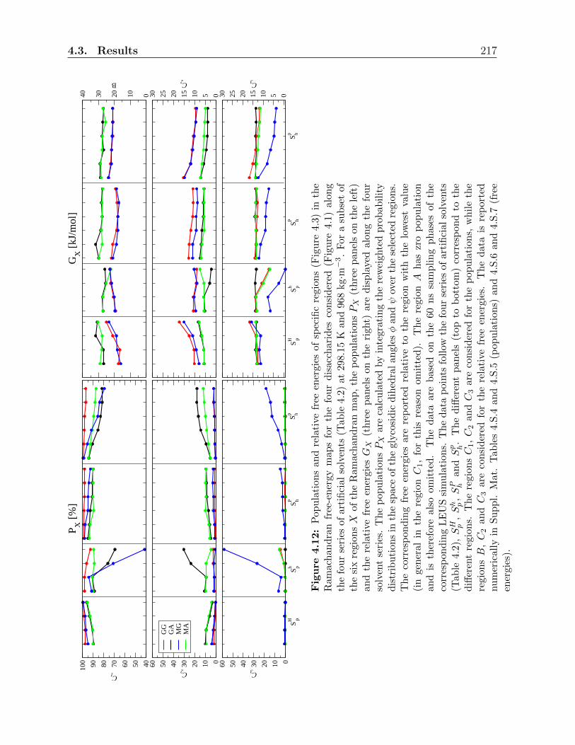
4.3. Results 217
PX
[%
]
405060708090100
C1
0102030405060
C2
GG
GA
MG
MA
SH p
Sh p
SP h
Sp h
0102030405060
C3G
X [
kJ/m
ol]
010203040
B
051015202530
C2
SH p
Sh p
SP h
Sp h
051015202530
C3
Figure
4.12:
Pop
ula
tion
san
dre
lati
vefr
eeen
ergi
esof
spec
ific
regi
ons
(Fig
ure
4.3)
inth
eR
amac
han
dra
nfr
ee-e
ner
gym
aps
for
the
fou
rd
isac
char
ides
con
sid
ered
(Fig
ure
4.1)
alo
ng
the
fou
rse
ries
ofar
tifi
cial
solv
ents
(Tab
le4.
2)at
298.
15K
and
968
kg·m−
3.
For
asu
bse
tof
the
six
regi
onsX
ofth
eR
amac
han
dra
nm
ap,
the
pop
ula
tion
sPX
(th
ree
pan
els
onth
ele
ft)
and
the
rela
tive
free
ener
giesGX
(th
ree
pan
els
onth
eri
ght)
are
dis
pla
yed
alon
gth
efo
ur
solv
ent
seri
es.
Th
ep
opu
lati
onsPX
are
calc
ula
ted
by
inte
grat
ing
the
rew
eigh
ted
pro
bab
ilit
yd
istr
ibu
tion
sin
the
spac
eof
the
glyco
sid
icd
ihed
ral
angl
esφ
andψ
over
the
sele
cted
regio
ns.
Th
eco
rres
pon
din
gfr
eeen
ergi
esar
ere
por
ted
rela
tive
toth
ere
gion
wit
hth
elo
wes
tva
lue
(in
gen
eral
inth
ere
gion
C1,
for
this
reas
onom
itte
d).
Th
ere
gion
Ah
aszr
op
opu
lati
on
and
isth
eref
ore
also
omit
ted
.T
he
dat
aar
eb
ased
onth
e60
ns
sam
pli
ng
ph
ases
of
the
corr
esp
ond
ing
LE
US
sim
ula
tion
s.T
he
dat
ap
oints
foll
owth
efo
ur
seri
esof
arti
fici
also
lven
ts(T
able
4.2)
,SH p
,Sh p,SP h
andSp h.
Th
ed
iffer
ent
pan
els
(top
tob
otto
m)
corr
esp
ond
toth
ed
iffer
ent
regi
ons.
The
regi
onsC
1,C
2an
dC
3ar
eco
nsi
der
edfo
rth
ep
opu
lati
ons,
wh
ile
the
regi
onsB
,C
2an
dC
3ar
eco
nsi
der
edfo
rth
ere
lati
vefr
eeen
ergi
es.
Th
ed
ata
isre
port
ednu
mer
ical
lyin
Su
pp
l.M
at.
Tab
les
4.S
.4an
d4.
S.5
(pop
ula
tion
s)an
d4.
S.6
and
4.S
.7(f
ree
ener
gies
).

218 Chapter 4. Disaccharides
and C3 (MG). In the opposite, GG seems to stabilize the global minimum in C1, that
keeps a population above 98% in all the solvents of the series. The H-bonding patterns of
GG, MG and GA are consistent with the conformational analysis, with a slight increase
in the numbers of both inter- and intraresidue H-bonds compensating for the decrease of
H-bonding with the solvent. For MA, the H-bonding pattern does not show significant
variations.
In the series Shp , the dielectric permittivity is decreased while the H-bonding capacity
is lower than that of water. For the four disaccharides, the trends along this series is
analogous to those observed along the series of physical solvents with decreasing polarity.
The appearance of a second minimum in region C3 for GG and MG, with the additional
third minimum in region C2 for the latter (metastable state separated by a high barrier
in the first case, stable state with a free energy comparable to the global minimum in the
second case) is compatible with the formation of a double H-bond between the rings. The
increase in the number of interresidue H-bonds and the additional increase in the number
of intraresidue H-bonds are again similar to the behaviour in the physical solvents of low
polarity. The formation of the second minimum in the region C2 for GA and MA (stable
state with a free energy comparable to the global minimum in the first case, metastable
state separated by a high barrier in the second case) is again associated with the increase
in the number of interresidue H-bonds (GA) and with an increase in the number of all
intraresidue H-bonds for both disaccharides.
In the series Sph, the H-bonding capacity is decreased while the dielectric permittivity
is lower than that of water. This evolution seems to have a similar qualitative effect
on the four compounds. However, a more careful analysis reveals that in this case, the
increase in the populations and the decrease in the relative free energy in regions C2 and C3
(effects anyway less significant in this series than the changes occurring when decreasing
the polarity for the physical solvents) are not always the consequence of the formation of

4.3. Results 219
a separate minimum, but can be seen as a broadening of the global minimum or of the
low free-energy basin present in that region. The variations in the H-bonding patterns of
the different disaccharides are similar, although less pronounced than the ones associated
to the decrease of the dielectric permittivity of the solvent. An important difference is the
constant occurrence of intraresidue H-bonding.
Figure 4.13: Numbers of H-bonds for the four disaccharides considered in the artificialsolvents at 298.15 K and 968 kg·m−3. The results are based on the 60 ns sampling phase ofthe corresponding LEUS simulations. Each bar represents the total number n of H-bonds,with different colors distinguishing interresidue H-bonds, intraresidue H-bonds, and solute-solvent H-bonds. The different bars for each solvent refer to one of the four disaccharides(Figure 4.1), that are identified by a box with the same color code as in Figure 4.7. Thebars follow the series of the artificial solvents, the series (a) SHp , (b) Shp , (c) SPh and (d) Sph(Table 4.2). The data is reported numerically in Suppl. Mat. Tables 4.S.8, 4.S.9, 4.S.10and 4.S.11.

220 Chapter 4. Disaccharides
4.4 Conclusions
Hydrogen-bonding (H-bonding) is often regarded as a determinant driving force in the
conformational preferences of (bio)molecules. However, the influence of H-bonding cannot
be discussed without consideration of the solute environment. When focusing on solvent-
exposed H-bonds in an aqueous environment, competition by the solvent molecules and
screening of the H-bonded interaction by the solvent dielectric response reduces their influ-
ence to that of a minor (possibly negligible or even, in some cases, adverse) conformational
driving as well as steering force. However, when the polarity of the solvent is decreased,
solvent-exposed H-bonds can become a very significant conformational steering force.
Qualitative or semi-quantitative evaluations of the influence of H-bonding on the con-
formational preferences of carbohydrates support this view in the context of monosacchar-
ides (see Chapter Chapter 3). However, for more complex systems such as oligosaccharides
or polysaccharides, the number of factors involved in the stability of specific conformations
can increase drastically. In the present study, MD simulations were used to analyze the
influence of H-bonding on the conformational properties of disaccharides. To this purpose
cellobiose and its epimers at C2 and C′3 were considered. The distributions of the glycosidic
dihedral angles φ and ψ were calculated in physical and artificial solvents of decreasing
polarity.
In an aqueous environment, the epimerization has only a very limited influence on the
conformational properties of the disaccharides considered, with no visible effects in case of
epimerization at C2. On the other hand, intramolecular the H-bonding pattern of the four
disaccharides is strongly modified by the epimerization, which inhibits the formation of
the typical interresidue H-bond (H′3→O5) often considered responsible for the equilibrium
conformation of cellobiose. In water, the lack of this intramolecular H-bond is easily
compensated for by a stronger interaction with the solvent molecules. This compensation
4.4. Conclusions 221
prevents possible large conformational changes necessary to recover the intramolecular H-
bond. The H-bonding is in this case an opportunistic consequence of the close proximity of
two H-bonding groups in a given epimer and conformation, and not a factor determining
the stability of this conformation for the epimer where it is possible.
When solvents of lower polarity are considered, significant conformational changes occur.
Alternative local minima appear in the free-energy maps, representing either metastable
or stable states depending on the specific epimer. The conformational changes can be
explained by the influence of intramolecular the H-bonding. However, several H-bonds are
possible, both intra- and interresidue. Their influence can act either in a cooperative way
or in a competitive way. In the first case, specific H-bonds concur to enhance the stability
of a specific conformation, shifting the conformational preference towards this specific
state. In the second case, incompatible H-bonds compete with each other, representing
in this case an adverse force towards this specific conformation. Therefore, in the case of
low-polarity solvents, solvent-exposed H-bonding can become as a very significant steering
force.
These considerations focus on the regions of the free-energy maps of the glycosidic di-
hedral angles φ and ψ that were sampled during the simulations, while vast areas of the
Ramachandran maps were not explored. The H-bond analysis reveals that the conforma-
tions corresponding to these excluded region would be the most favorable ones in terms of
the number of H-bonds compatible with these values of the dihedral angles. However, the
same conformations involve steric clashes between atoms of the two residue that drastically
increase their free energy. The evaluation of this aspect requires additional work.

222 Chapter 4. Disaccharides
Figure
A.14:
Fre
e-en
ergy
map
sG
(φ,ψ
)in
the
spac
eof
the
glyco
sid
icd
ihed
ral
angle
sφ
an
dψ
.T
he
map
sar
ed
isp
laye
dfo
rG
lcp
-α(1→
4)-G
lcp
-α(G
Gα,α
-mal
tose
;fo
ur
pan
els
on
the
left
)an
dG
lcp
-β(1→
4)-G
lcp
-β(G
Gβ,β
-cel
lob
iose
;fo
ur
pan
els
onth
eri
ght)
.In
both
case
s,th
efo
ur
pan
els
corr
esp
ond
tosi
mu
lati
ons
invo
lvin
gre
stra
inin
gof
the
two
rin
gs
insp
ecifi
cch
air
con
form
atio
ns,
nam
ely
4C
1-4
C1,
1C
4-4
C1,
4C
1-1
C4
and
1C
4-1
C4,
wh
ere
the
two
sym
bols
spec
ify
the
con
form
atio
nof
the
firs
tan
dth
ese
con
dri
ng,
resp
ecti
vely
.T
he
free
ener
gies
wer
eca
lcu
late
db
ased
onth
e60
ns
sam
pli
ng
ph
ase
ofth
eco
rres
pon
din
gL
EU
Ssi
mu
lati
on
sat
1b
aran
d29
8.15
Kin
wat
er.
Th
em
aps
are
anch
ored
toG
=0
kJ
mol−
1
atth
elo
cati
onof
thei
rgl
obal
min
imu
m,
and
the
valu
eofG
atgr
idp
oints
that
wer
en
ever
vis
ited
du
rin
gth
esi
mu
lati
ons
isar
bit
rari
lyse
tto
the
max
imal
valu
eGmax
(wh
ich
isab
ou
t50
kJ
mol−
1h
ere
inall
case
s).

4.A. Influence of the ring conformation 223
4.A Influence of the ring conformation
The simulations reported in this chapter were all performed with dihedral-angle restraints
applied to the two rings so as to ensure a 4C1 chair conformation throughout the simula-
tions. The influence of possible flips in the ring conformations is analyzed in this appendix
focusing on the GG disaccharide (β-cellobiose, named here GGβ). The α(1→4)-linked Glc-
based disaccharide with α-anomery at the reducing residue, namely Glcp-α(1→4)-Glcp-α
(GGα, α-mannose) is also considered.
LEUS simulations of the GGβ and GGα disaccharides with the two rings restrained in
different conformations (4C1-4C1, 1C4-4C1, 4C1-1C4 or 1C4-1C4) were performed in water.
All the parameters in the LEUS simulations were the same as for the main simulations.
These simulations are labelled LEUS-R1-R2, R1 and R2 referring to the conformation of
the two rings.
The free-energy maps obtained from simulations of GGα and GGβ in water with rings
restrained in different conformations are shown in Figure A.14. As suggested in Ref.329,
the influence of the ring conformation on the glycosidic linkage properties is limited when
focusing on the equilibrium configuration (φ ' 300 and ψ ' 60). The only significant
difference is observed for GGβ, where the global minimum is shifted by about 60 in ψ
when restraining the second ring in an inverted-chair conformation. However, the extent
of the space visited and the details of free-energy map in the alternative metastable states
reveal that the effect of the puckering is not completely negligible.
In a study concerning the effect of the solvent on the conformational properties of the
glycosidic linkage, any discussion would be complicated by the presence of alternative ring
conformations. For this reason, the ring conformations were restrained to 4C1 for both
rings during the LEUS simulations as reported in the main text (Section 4.2.3). In the
absence of restraints (data not shown), several simulations evidenced the occurrence of a

224 Chapter 4. Disaccharides
transition, with a higher propensity of the second ring to flip. The reasons for the tendency
to a distortion in the second ring were further investigated and the results of this analysis
led to the publication of a patch for the 56A6CARBO force field (56A6CARBO R). For more
details see Ref246.
Results from unrestrained simulations that did not evidence a transition in the ring
conformation and from restrained simulations were compared and suggested that the effect
of the restraints on the glycosidic-linkage properties can be considered negligible (relative
to a situation without restraints where no flip occurs).

4.S.1. Supplementary Material 225
4.S.1 Supplementary Material
Comp. Reg. H2O DMSO CH3OH CHCl3 CCl4
GG
A 0.00 0.00 0.00 0.00 0.00B 0.04 0.04 0.04 0.01 0.05C 99.96 99.96 99.96 99.99 99.95C1 98.88 97.95 98.97 96.10 91.56C2 0.73 1.38 0.64 2.20 3.76C3 0.35 0.63 0.35 1.69 4.63
GA
A 0.00 0.00 0.00 0.00 0.00B 0.00 0.00 0.00 0.00 0.01C 100.00 100.00 100.00 100.00 99.99C1 93.00 89.04 91.89 76.93 75.86C2 6.51 10.58 7.53 22.77 23.59C3 0.49 0.38 0.58 0.29 0.54
MG
A 0.00 0.00 0.00 0.00 0.00B 0.03 0.04 0.05 0.00 0.00C 99.97 99.96 99.95 100.00 100.00C1 97.84 88.33 94.89 56.58 60.45C2 1.00 2.61 1.12 1.23 0.42C3 1.13 9.02 3.95 42.18 39.12
MA
A 0.00 0.00 0.00 0.00 0.00B 0.00 0.00 0.00 0.01 0.00C 100.00 100.00 100.00 99.99 100.00C1 92.68 94.76 97.07 90.63 93.90C2 6.84 4.05 2.19 4.86 1.97C3 0.47 1.20 0.73 4.51 4.13
Table 4.S.1: Populations (in percent) of specific regions (Figure 4.3) in the Ramachandranfree-energy maps for the four disaccharides considered (Figure 4.1) along the series of phys-ical solvents at 298.15 K and 1 bar. The results are based on the 60 ns sampling phase ofthe corresponding LEUS simulations. The populations PX are calculated by integrating thereweighted probability distributions in the space of the glycosidic dihedral angles φ and ψover the selected regions. The entries follow the series of physical solvents (Table 4.1) inorder of decreasing polarity and refer to the four disaccharides considered (GG, GA, MG,MA). The regions considered are A, B, and C and C1, C2, as well as the subregions C3.Note that the populations of C1, C2 and C3 sum up to that of C, and the populations of A,B and C sum up to 100%. The data is illustrated graphically in Figure 4.7.

226 Chapter 4. Disaccharides
Com
p.
Reg
.H
2O
DM
SO
CH
3O
HC
HC
l 3C
Cl 4
GX
GX
(φX
,ψX
)GX
GX
(φX
,ψX
)GX
GX
(φX
,ψX
)GX
GX
(φX
,ψX
)GX
GX
(φX
,ψX
)
GG
B19.2
18.9
(290,3
20)
19.1
18.7
(294,3
18)
19.4
19.6
(288,3
20)
21.8
22.5
(260,3
02)
18.5
18.7
(262,3
04)
C1
0.0
0.0
(294,1
16)
0.0
0.0
(284,1
12)
0.0
0.0
(292,1
16)
0.0
0.0
(270,1
12)
0.0
0.0
(274,1
08)
C2
12.2
--
10.6
--
12.5
--
9.4
--
7.9
--
C3
14.0
--
12.5
12.7
(52,1
14)
14.0
15.6
(38,1
18)
10.0
9.3
(56,1
16)
7.4
6.4
(54,1
18)
GA
B30.7
28.5
(284,3
18)
27.7
24.9
(282,3
04)
26.4
25.2
(282,3
12)
25.0
23.8
(282,3
12)
23.1
21.7
(280,3
10)
C1
0.0
0.0
(290,1
06)
0.0
0.0
(290,1
04)
0.0
0.0
(290,1
02)
0.0
--
0.0
--
C2
6.6
--
5.3
--
6.2
--
3.0
0.0
(236,
82)
2.9
0.0
(232,
80)
C3
13.0
--
13.5
--
12.6
--
13.8
--
12.2
--
MG
B20.4
19.7
(288,3
20)
18.9
18.2
(286,3
20)
19.0
18.5
(288,3
14)
23.4
21.9
(288,3
20)
24.8
23.3
(288,3
30)
C1
0.0
0.0
(284,1
14)
0.0
0.0
(292,1
10)
0.0
0.0
(286,1
10)
0.0
0.0
(286,1
12)
0.0
0.0
(292,1
14)
C2
11.4
11.4
(188,
90)
8.7
8.0
(186,
88)
11.0
9.7
(192,
90)
9.5
7.7
(188,
90)
12.3
9.7
(190,
84)
C3
11.1
--
5.6
6.2
(34,1
14)
7.9
7.6
(350,1
10)
0.7
0.7
(34,1
16)
1.1
0.5
(6,1
06)
MA
B29.4
27.5
(290,3
10)
31.5
29.4
(288,3
06)
30.0
28.6
(280,3
00)
23.7
22.1
(280,3
14)
24.7
24.0
(284,3
02)
C1
0.0
0.0
(296,1
06)
0.0
0.0
(302,1
08)
0.0
0.0
(302,1
06)
0.0
0.0
(298,1
06)
0.0
0.0
(302,1
04)
C2
6.4
--
7.8
8.1
(202,
76)
9.4
--
7.2
5.6
(190,
82)
9.6
8.4
(194,
80)
C3
13.1
--
10.8
--
12.1
--
7.4
7.1
(36,
82)
7.7
8.2
(6,
78)
Table
4.S.2:
Fre
een
ergi
es(i
nkJ
mol−
1)
and
pos
itio
ns
ofth
em
inim
a(i
nd
egre
es)
ofsp
ecifi
cre
gion
s(F
igu
re4.
3)d
efin
edin
the
Ram
ach
and
ran
free
-en
ergy
map
sfo
rth
efo
ur
dis
acch
ari
des
con
sid
ered
(Fig
ure
4.1)
alon
gth
ese
ries
ofpysi
calso
lven
tsat
298.
15K
and
1b
ar.
Th
ere
sult
sar
eb
ased
onth
e60
ns
sam
pli
ng
ph
ase
ofth
eco
rres
pon
din
gL
EU
Ssi
mu
lati
ons.
Th
efr
eeen
ergi
es,
calc
ula
ted
eith
erfo
rth
est
ateX
(GX
)or
atth
eco
rres
pon
din
glo
cal
min
imu
m(G
Xat
the
pos
itio
nφX
,ψX
),ar
ere
por
ted
rela
tive
toth
eco
rres
pon
din
glo
wes
tva
lue
(in
the
regi
onC
1ex
cep
tfo
rG
Ain
CC
l 4,
wh
ere
itis
inre
gion
C2).
Th
ere
gion
An
ever
pre
sents
am
inim
um
and
isth
eref
ore
omit
ted
.T
he
min
imu
min
the
regi
onC
corr
esp
ond
toth
elo
wes
tof
the
min
ima
inth
esu
bre
gion
sC
1,C
2orC
3.
Th
ere
gion
sco
nsi
der
edar
eB
,C
1,C
2an
dC
3.
Th
een
trie
sfo
llow
the
seri
esof
physi
cal
solv
ents
(Tab
le4.
1)in
ord
erof
dec
reas
ing
pola
rity
and
refe
rto
the
fou
rd
isac
char
ides
con
sid
ered
(GG
,G
A,
MG
,M
A).
Th
ed
ata
isil
lust
rate
dgr
aph
ical
lyin
Fig
ure
4.7.
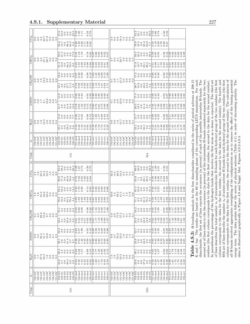
4.S.1. Supplementary Material 227
Cmp.
A.
H2O
DM
SO
CH
3OH
CHCl 3
CCl 4
Cmp.
A.
H2O
DM
SO
CH
3OH
CHCl 3
CCl 4
GG
O2-O
3′
0.0
0.3
0.1
1.5
4.1
GA
O2-O
3′
0.0
0.0
0.0
0.0
0.0
O6-O
3′
1.7
3.5
2.5
1.8
1.9
O6-O
3′
0.0
0.0
0.0
0.0
0.0
O5-O
3′
67.9
86.4
86.0
91.0
85.5
O5-O
3′
1.0
1.7
1.6
2.3
2.2
O1-O
3′
50.3
51.7
55.9
56.0
55.2
O1-O
3′
12.5
8.1
12.6
27.1
22.7
O2-O
6′
1.8
10.8
8.7
63.3
53.5
O2-O
6′
3.8
18.8
9.0
60.7
51.9
O5-O
6′
0.0
0.0
0.0
0.4
1.0
O5-O
6′
0.0
0.0
0.0
0.0
0.0
O6-O
6′
0.0
0.1
0.0
0.9
2.3
O6-O
6′
0.0
0.0
0.0
0.0
0.0
O1-O
6′
0.5
2.3
2.4
6.3
2.0
O1-O
6′
0.4
5.7
2.2
5.2
3.5
O2-O
334.0
38.2
38.1
52.3
42.5
55.1
78.6
84.4
80.8
85.0
O2-O
335.1
15.8
41.7
14.8
44.1
18.2
81.2
50.0
83.2
47.6
O2-O
13.7
4.4
3.6
3.8
3.1
4.5
19.4
34.2
17.2
39.2
O2-O
13.5
5.9
3.9
8.0
4.6
6.9
12.6
31.3
13.7
33.9
O2-O
50.0
0.0
0.0
0.0
0.0
0.0
0.0
0.0
0.0
0.0
O2-O
50.0
0.0
0.0
0.0
0.0
0.0
0.0
0.0
0.0
0.0
O3-O
439.4
0.0
41.4
0.0
45.8
0.0
84.2
0.0
84.8
0.0
O3-O
438.3
0.0
41.8
0.0
47.7
0.0
84.3
0.0
86.2
0.0
O4-O
62.6
0.0
3.7
0.0
5.0
0.0
79.4
0.0
78.6
0.0
O4-O
62.6
0.0
10.4
0.0
11.5
0.0
79.5
0.0
84.5
0.0
O6-O
53.9
8.0
8.7
5.2
3.2
8.3
3.4
14.4
4.2
20.3
O6-O
55.0
7.7
12.8
4.7
4.9
8.3
8.0
17.9
6.2
23.5
O1-m
ol
0.54
0.04
0.58
0.04
0.61
0.04
0.82
0.34
0.74
0.39
O1-m
ol
0.16
0.06
0.18
0.08
0.19
0.07
0.45
0.31
0.40
0.34
O2-m
ol
0.39
0.42
0.53
0.57
0.55
0.60
1.63
1.70
1.56
1.67
O2-m
ol
0.42
0.15
0.64
0.22
0.58
0.22
1.55
1.12
1.49
1.20
O3-m
ol
1.44
1.57
1.46
1.96
1.54
2.00
2.00
2.86
2.05
2.74
O3-m
ol
1.44
0.22
1.52
0.24
1.56
0.29
2.06
1.10
2.06
1.11
O4-m
ol
0.42
-0.45
-0.51
-1.64
-1.63
-O4-m
ol
0.41
-0.52
-0.59
-1.64
-1.71
-O5-m
ol
0.04
0.08
0.09
0.05
0.03
0.08
0.04
0.14
0.05
0.20
O5-m
ol
0.05
0.08
0.13
0.05
0.05
0.08
0.08
0.18
0.06
0.24
O6-m
ol
0.04
0.10
0.07
0.18
0.08
0.20
0.83
0.85
0.84
0.79
O6-m
ol
0.03
0.12
0.10
0.29
0.12
0.19
0.80
0.84
0.85
0.79
O1-svt
0.09
2.10
0.00
0.95
0.01
1.73
0.01
0.12
O1-svt
0.19
2.10
0.00
0.96
0.04
1.64
0.02
0.07
O2-svt
1.83
1.77
0.80
0.58
1.17
1.16
0.03
0.06
O2-svt
1.78
1.89
0.76
0.88
1.16
1.45
0.03
0.06
O3-svt
1.71
1.20
0.83
0.16
1.10
0.43
0.04
0.03
O3-svt
1.72
1.77
0.81
0.85
1.10
1.26
0.03
0.05
O4-svt
1.72
0.00
0.75
0.00
1.08
0.00
0.03
0.00
O4-svt
1.74
0.00
0.73
0.00
1.01
0.00
0.03
0.00
O5-svt
0.03
0.40
0.00
0.00
0.00
0.13
0.00
0.04
O5-svt
0.14
0.44
0.00
0.00
0.04
0.13
0.01
0.02
O6-svt
2.18
2.12
0.90
0.88
1.67
1.68
0.10
0.06
O6-svt
2.24
2.16
0.88
0.81
1.71
1.68
0.09
0.07
MG
O2-O
3′
1.3
9.9
4.4
43.6
42.4
MA
O2-O
3′
0.0
0.1
0.1
2.7
2.3
O6-O
3′
1.9
2.7
2.0
1.2
0.2
O6-O
3′
0.0
0.0
0.0
0.0
0.0
O5-O
3′
72.5
76.2
77.6
49.3
46.0
O5-O
3′
1.0
0.9
1.1
2.1
0.8
O1-O
3′
53.3
53.5
57.1
41.5
54.3
O1-O
3′
15.7
25.6
21.5
29.7
16.4
O2-O
6′
0.2
1.8
0.7
1.1
0.3
O2-O
6′
0.5
1.5
0.5
3.6
1.5
O5-O
6′
0.0
0.2
0.1
1.3
0.4
O5-O
6′
0.0
0.0
0.0
0.0
0.0
O6-O
6′
0.0
1.5
0.3
11.8
5.4
O6-O
6′
0.0
0.0
0.0
0.0
0.0
O1-O
6′
0.0
0.1
0.1
0.6
0.3
O1-O
6′
0.1
0.5
0.3
1.5
0.4
O2-O
322.6
38.1
24.9
52.7
25.9
54.2
71.1
87.4
63.9
88.6
O2-O
323.1
15.7
26.0
17.4
28.7
17.5
71.9
56.3
78.9
54.2
O2-O
15.9
4.5
5.9
3.4
5.0
4.5
8.3
35.6
1.1
40.6
O2-O
16.9
5.8
19.5
6.0
10.8
6.2
19.7
30.2
35.5
32.1
O2-O
50.0
0.0
0.0
0.0
0.0
0.0
0.0
0.0
0.0
0.0
O2-O
50.0
0.0
0.0
0.0
0.0
0.0
0.0
0.0
0.0
0.0
O3-O
437.6
0.0
42.5
0.0
43.2
0.0
81.3
0.0
83.1
0.0
O3-O
436.1
0.0
41.4
0.0
43.6
0.0
83.1
0.0
85.4
0.0
O4-O
62.6
0.0
9.3
0.0
12.8
0.0
76.5
0.0
90.5
0.0
O4-O
63.8
0.0
9.0
0.0
12.6
0.0
86.5
0.0
84.8
0.0
O6-O
53.9
8.8
6.8
5.3
3.8
7.0
9.9
41.3
4.1
48.9
O6-O
55.5
7.9
7.6
5.2
5.2
9.2
4.7
38.4
5.7
39.6
O1-m
ol
0.59
0.05
0.60
0.03
0.62
0.05
0.50
0.36
0.56
0.41
O1-m
ol
0.23
0.06
0.46
0.06
0.33
0.06
0.51
0.30
0.52
0.32
O2-m
ol
0.30
0.43
0.43
0.56
0.36
0.59
1.24
1.23
1.08
1.29
O2-m
ol
0.31
0.22
0.47
0.23
0.40
0.24
0.98
0.87
1.18
0.86
O3-m
ol
1.37
1.67
1.38
1.95
1.42
1.95
2.13
2.23
2.40
2.31
O3-m
ol
1.37
0.32
1.36
0.44
1.42
0.40
2.11
0.91
2.00
0.74
O4-m
ol
0.40
-0.52
-0.56
-1.58
-1.74
-O4-m
ol
0.40
-0.50
-0.56
-1.70
-1.70
-O5-m
ol
0.04
0.09
0.07
0.05
0.04
0.07
0.11
0.41
0.04
0.49
O5-m
ol
0.06
0.08
0.08
0.05
0.05
0.09
0.05
0.38
0.06
0.40
O6-m
ol
0.08
0.09
0.20
0.09
0.19
0.08
0.99
0.56
1.00
0.55
O6-m
ol
0.09
0.09
0.17
0.07
0.18
0.10
0.91
0.44
0.91
0.42
O1-svt
0.08
2.11
0.00
0.95
0.01
1.69
0.01
0.10
O1-svt
0.15
2.11
0.00
0.96
0.02
1.69
0.01
0.08
O2-svt
1.91
1.79
0.85
0.59
1.44
1.17
0.05
0.04
O2-svt
1.91
1.90
0.91
0.85
1.50
1.48
0.06
0.06
O3-svt
1.75
1.12
0.82
0.14
1.26
0.55
0.05
0.03
O3-svt
1.77
1.76
0.76
0.88
1.25
1.29
0.04
0.05
O4-svt
1.75
0.00
0.76
0.00
1.08
0.00
0.04
0.00
O4-svt
1.75
0.00
0.72
0.00
1.08
0.00
0.03
0.00
O5-svt
0.04
0.40
0.00
0.00
0.01
0.12
0.00
0.02
O5-svt
0.17
0.44
0.00
0.00
0.03
0.13
0.01
0.02
O6-svt
2.20
2.14
0.85
0.93
1.62
1.69
0.08
0.08
O6-svt
2.22
2.16
0.88
0.93
1.66
1.72
0.08
0.08
Table
4.S.3:
H-b
on
din
gan
aly
sis
for
the
fou
rd
isacc
hari
des
con
sid
ered
inth
ese
ries
of
pysi
cal
solv
ents
at
298.1
5K
an
d1
bar.
Th
ere
sult
sare
base
don
the
60
ns
sam
plin
gp
hase
of
the
corr
esp
on
din
gL
EU
Ssi
mu
lati
on
s.F
or
each
dis
acc
hari
de,
the
firs
tse
tof
lin
esre
port
sth
eocc
ure
nce
(in
per
cent)
of
each
of
the
poss
ible
inte
rres
idu
eH
-bon
ds.
Th
ese
con
dse
tof
lin
esre
fers
toth
eth
eocc
ure
nce
(in
per
cent)
of
the
intr
are
sid
ue
H-b
on
ds
con
sid
ered
sep
ara
tely
for
the
two
resi
du
es(t
he
firs
tco
lum
nco
rres
pon
ds
toth
ed
ata
for
the
firs
tre
sid
ue,
the
seco
nd
toth
ed
ata
for
the
seco
nd
resi
du
e).
Inp
are
nth
esis
the
per
centa
ge
of
the
hyd
rogen
bon
ds
that
involv
eth
efi
rst
ato
mas
ad
on
or
isre
port
ed.
Th
eth
ird
set
of
lin
esd
escr
ibes
the
tota
lnu
mb
erni
of
intr
am
ole
cula
rH
-bon
ds
for
each
hyd
roxyl
gro
up
of
the
two
resi
du
es(t
he
firs
tco
lum
nco
rres
pon
ds
toth
ed
ata
for
the
firs
tre
sid
ue,
the
seco
nd
toth
ed
ata
for
the
seco
nd
resi
du
e).
Th
efo
urt
han
dfi
fth
set
of
lin
esd
escr
ibe
the
nu
mb
erns
of
solu
te-s
olv
ent
H-b
on
ds
for
each
hydro
xyl
gro
up
of
the
two
resi
du
es(t
he
firs
tco
lum
nco
rres
pon
ds
toth
ed
ata
for
the
firs
tre
sid
ue,
the
seco
nd
toth
ed
ata
for
the
seco
nd
resi
du
e).
Th
eca
lcu
lati
on
of
all
H-b
on
ds
involv
edap
pro
pri
ate
rew
eighti
ng
of
the
con
figu
rati
on
sso
as
tore
move
the
effec
tof
the
bia
sin
gp
ote
nti
al
ener
gy
term
.T
he
data
poin
tsfo
llow
the
seri
esof
physi
cal
solv
ents
(Tab
le4.1
)in
ord
erof
dec
reasi
ng
pola
rity
.T
he
data
isillu
stra
ted
gra
ph
icall
yin
Fig
ure
4.8
an
dS
up
pl.
Mat.
Fig
ure
s4.S
.2-4
.S.4
.

228 Chapter 4. Disaccharides
Cmp.Series SHp Series Shp
Reg. W0.81.4 W0.9
1.2 W1.01.0 W1.5
0.5 Reg. W0.51.4 W0.8
0.9 W0.70.6 W0.3
0.5
A 0.00 0.00 0.00 0.00 A 0.00 0.00 0.00 0.00B 0.09 0.12 0.02 0.00 B 0.04 0.02 0.01 0.01C 99.91 99.88 99.98 100.00 C 99.96 99.98 99.99 99.99C1 97.67 97.73 98.93 99.78 C1 98.16 98.31 96.32 92.57C2 1.63 1.53 0.63 0.10 C2 1.37 1.29 2.38 2.39C3 0.61 0.61 0.42 0.12 C3 0.43 0.37 1.29 5.03
GA
A 0.00 0.00 0.00 0.00 A 0.00 0.00 0.00 0.00B 0.00 0.00 0.00 0.00 B 0.00 0.00 0.00 0.00C 100.00 100.00 100.00 100.00 C 100.00 100.00 100.00 100.00C1 89.79 90.55 93.74 96.13 C1 88.90 90.54 76.16 69.43C2 9.75 9.10 5.83 3.40 C2 10.76 9.07 23.55 30.26C3 0.45 0.36 0.42 0.48 C3 0.34 0.39 0.28 0.31
MG
A 0.00 0.00 0.00 0.00 A 0.00 0.00 0.00 0.00B 0.15 0.06 0.05 0.01 B 0.03 0.03 0.01 0.00C 99.85 99.94 99.95 99.99 C 99.97 99.97 99.99 100.00C1 94.98 96.82 97.74 99.59 C1 91.43 94.20 71.11 41.27C2 3.85 2.30 1.17 0.23 C2 1.99 1.48 1.90 0.66C3 1.02 0.82 1.04 0.18 C3 6.54 4.29 26.98 58.07
MA
A 0.00 0.00 0.00 0.00 A 0.00 0.00 0.00 0.00B 0.00 0.00 0.00 0.00 B 0.00 0.00 0.00 0.01C 100.00 100.00 100.00 100.00 C 100.00 100.00 100.00 99.99C1 90.25 90.50 93.04 95.57 C1 90.01 90.60 89.04 89.58C2 9.30 9.07 6.51 4.03 C2 9.52 9.00 9.32 4.46C3 0.46 0.42 0.45 0.40 C3 0.47 0.39 1.64 5.95
Table 4.S.4: Populations (in percent) of specific regions (Figure 4.3) in the Ramachandranfree-energy maps for the four disaccharides considered (see Fig. 4.1) along the series SHp(left) and Shp (right) of artificial solvents at 298.15 K and 968 kg·m−3. The results are basedon the 60 ns sampling phases of the corresponding LEUS simulations. The populations PXare calculated by integrating the reweighted probability distributions in the space of theglycosidic dihedral angles φ and ψ over the selected regions. The entries follow two of thefour series of artificial solvents (Table 4.2) in order of decreasing dielectric permittivity: onthe left the series SHp , on the right the Shp and refer to the four disaccharides considered(GG, GA, MG, MA). The regions considered are A, B, and C as well as subregions C1,C2 and C3. Note that the populations of C1, C2 and C3 sum up to that of C, and thepopulations of A, B and C sum up to 100%. The data is illustrated graphically in Figure4.12.

4.S.1. Supplementary Material 229
Com
p.
Ser
iesSP h
Ser
iesSp h
Reg
.W
1.1
0.9
W1.0
1.0
W0.8
1.1
W0.7
1.2
W0.6
1.4
W0.5
1.5
Reg
.W
1.5
0.4
W1.2
0.5
W1.1
0.5
W0.8
0.7
W0.6
0.9
W0.4
1.3
GG
A0.
000.
000.
000.0
00.0
00.0
0A
0.0
00.0
00.0
00.0
00.0
00.0
0B
0.01
0.02
0.05
0.0
70.0
60.0
4B
0.0
10.0
10.0
20.0
20.0
20.0
2C
99.9
999
.98
99.9
599.9
399.9
499.9
6C
99.9
999.9
999.9
899.9
899.9
899.9
8C
199
.07
98.9
398
.65
98.1
898.0
798.2
3C
199.6
698.9
298.4
998.1
097.0
497.0
9C
20.
560.
630.
861.2
31.3
01.2
8C
20.2
10.8
41.0
91.3
92.1
22.0
7C
30.
350.
420.
440.5
20.5
60.4
5C
30.1
20.2
30.4
10.4
90.8
20.8
2
GA
A0.
000.
000.
000.0
00.0
00.0
0A
0.0
00.0
00.0
00.0
00.0
00.0
0B
0.00
0.00
0.00
0.0
00.0
00.0
0B
0.0
00.0
00.0
00.0
00.0
00.0
0C
100.
0010
0.00
100.
00100.0
0100.0
0100.0
0C
100.0
0100.0
0100.0
0100.0
0100.0
0100.0
0C
194
.95
93.7
492
.78
91.1
590.8
490.2
1C
194.1
990.5
385.4
683.1
581.5
781.8
3C
24.
685.
836.
808.5
48.7
39.4
2C
25.4
09.1
014.1
516.5
118.0
717.8
1C
30.
380.
420.
420.3
10.4
30.3
7C
30.4
10.3
70.3
90.3
30.3
60.3
5
MG
A0.
000.
000.
000.0
00.0
00.0
0A
0.0
00.0
00.0
00.0
00.0
00.0
0B
0.02
0.05
0.08
0.0
80.0
90.0
5B
0.0
10.0
10.0
10.0
20.0
20.0
2C
99.9
899
.95
99.9
299.9
299.9
199.9
5C
99.9
999.9
999.9
999.9
899.9
899.9
8C
198
.07
97.7
495
.14
94.9
493.9
792.6
3C
199.0
895.4
491.8
185.7
283.8
579.4
2C
21.
161.
172.
242.1
82.8
42.3
9C
20.2
50.8
01.1
01.3
91.8
52.0
9C
30.
751.
042.
552.8
03.1
04.9
3C
30.6
63.7
57.0
712.8
714.2
818.4
7
MA
A0.
000.
000.
000.0
00.0
00.0
0A
0.0
00.0
00.0
00.0
00.0
00.0
0B
0.00
0.00
0.00
0.0
00.0
00.0
0B
0.0
00.0
00.0
00.0
00.0
00.0
0C
100.
0010
0.00
100.
00100.0
0100.0
0100.0
0C
100.0
0100.0
0100.0
0100.0
0100.0
0100.0
0C
193
.72
93.0
489
.66
90.4
190.0
290.3
5C
194.5
692.6
590.6
489.6
188.3
087.2
3C
25.
846.
519.
959.2
49.6
39.2
1C
25.0
96.9
08.7
99.7
210.9
211.8
7C
30.
440.
450.
380.3
50.3
50.4
4C
30.3
50.4
50.5
60.6
70.7
80.8
9
Table
4.S.5:
Pop
ula
tion
s(i
np
erce
nt)
of
spec
ific
regio
ns
(Fig
ure
4.3
)in
the
Ram
ach
an
dra
nfr
ee-
ener
gym
aps
for
the
fou
rd
isacc
hari
des
con
sid
ered
(see
Fig
.4.1
)alo
ng
the
seri
esSP h
(lef
t)an
dSp h
(rig
ht)
ofar
tifi
cial
solv
ents
at
298.1
5K
an
d968
kg·m
−3.
Th
ere
sult
sare
base
don
the
60
ns
sam
pli
ng
ph
ases
ofth
eco
rres
pon
din
gL
EU
Ssi
mu
lati
on
s.T
he
pop
ula
tion
sPX
are
calc
ula
ted
by
inte
gra
tin
gth
ere
wei
ghte
dp
rob
abil
ity
dis
trib
uti
on
sin
the
space
of
the
gly
cosi
dic
dih
edra
lan
gle
sφ
an
dψ
over
the
sele
cted
regi
ons.
Th
een
trie
sfo
llow
two
of
the
fou
rse
ries
of
art
ifici
al
solv
ents
(Tab
le4.2
)in
ord
erof
dec
reas
ing
die
lect
ric
per
mit
tivit
y:
on
the
left
the
seri
esSP h
,on
the
right
theSp h
an
dre
fer
toth
efo
ur
dis
acch
arid
esco
nsi
der
ed(G
G,
GA
,M
G,
MA
).T
he
regio
ns
con
sid
ered
areA
,B
,an
dC
as
wel
las
the
sub
regi
onsC
1,C
2an
dC
3.
Note
that
the
pop
ula
tion
sofC
1,C
2an
dC
3su
mu
pto
that
of
C,
and
the
pop
ula
tion
sofA
,B
an
dC
sum
up
to100%
.T
he
data
isil
lust
rate
dgra
ph
icall
yin
Fig
ure
4.12
.

230 Chapter 4. Disaccharides
Cmp. Reg.
Series SHp
W0.81.4 W0.9
1.2 W1.01.0 W1.5
0.5
GX GX (φX , ψX) GX GX (φX , ψX) GX GX (φX , ψX) GX GX (φX , ψX)
GG
B 17.4 16.2 (284,318) 16.6 16.6 (288,316) 21.1 20.4 (288,318) 25.0 25.2 (286,316)
C1 0.0 0.0 (300,120) 0.0 0.0 (296,118) 0.0 0.0 (294,120) 0.0 0.0 (294,116)
C2 10.1 - - 10.3 - - 12.5 - - 17.2 - -
C3 12.6 - - 12.6 - - 13.5 - - 16.6 - -
GA
B 26.7 24.7 (284,310) 26.9 25.3 (292,308) 31.8 27.6 (292,310) 30.8 29.1 (282,312)
C1 0.0 0.0 (292,108) 0.0 0.0 (294,104) 0.0 0.0 (292,108) 0.0 0.0 (290,104)
C2 5.5 - - 5.7 - - 6.9 - - 8.3 - -
C3 13.1 - - 13.7 - - 13.4 - - 13.2 - -
MG
B 15.9 14.3 (294,318) 18.2 17.6 (292,318) 18.6 17.9 (294,314) 23.4 22.6 (290,314)
C1 0.0 0.0 (300,120) 0.0 0.0 (294,112) 0.0 0.00 (290,114) 0.0 0.0 (296,114)
C2 7.9 7.7 (204, 86) 9.3 9.7 (208, 92) 11.0 11.1 (190, 90) 15.1 15.5 (230, 96)
C3 11.2 - - 11.8 - - 11.3 - - 15.7 - -
MA
B 29.0 27.1 (292,312) 27.9 26.4 (288,308) 27.7 26.2 (286,314) 30.2 28.6 (290,312)
C1 0.0 0.0 (292,102) 0.0 0.0 (292,106) 0.0 0.0 (296,106) 0.0 0.0 (292,102)
C2 5.6 - - 5.7 - - 6.6 - - 7.8 6.7 (230, 74)
C3 13.1 - - 13.3 - - 13.2 - - 13.6 - -
Cmp. Reg.
Series Shp
W0.51.4 W0.8
0.9 W0.70.6 W0.5
0.3
GX GX (φX , ψX) GX GX (φX , ψX) GX GX (φX , ψX) GX GX (φX , ψX)
GG
B 19.2 19.0 (282,316) 20.7 20.9 (284,314) 22.4 22.8 (264,304) 22.8 23.4 (264,306)
C1 0.0 0.0 (288,110) 0.0 0.0 (288,114) 0.0 0.0 (278,108) 0.0 0.0 (278,108)
C2 10.6 9.3 (210, 94) 10.7 9.8 (224, 88) 9.2 7.5 (222, 94) 9.1 - -
C3 13.5 13.8 ( 56,118) 13.8 14.9 ( 52,120) 10.7 9.0 ( 46,120) 7.2 5.7 ( 48,118)
GA
B 27.1 25.5 (280,314) 27.5 26.1 (284,306) 25.6 24.4 (282,310) 26.0 24.5 (282,302)
C1 0.0 0.0 (284,100) 0.0 0.0 (286,102) 0.0 1.07 (234, 88) 0.0 0.4 (232, 84)
C2 5.2 3.0 (228, 78) 5.7 3.3 (222, 82) 2.9 0.0 (230, 82) 2.1 0.0 (222, 82)
C3 13.8 - - 13.5 - - 13.9 - - 13.4 - -
MG
B 19.6 18.7 (288,316) 20.1 20.0 (290,312) 21.7 21.9 (288,318) 22.8 23.3 (284,316)
C1 0.0 0.0 (294,114) 0.0 0.0 (288,112) 0.0 0.0 (292,114) 0.0 0.9 (290,112)
C2 9.5 8.5 (186, 90) 10.3 10.2 (192, 90) 9.0 7.6 (188, 90) 10.3 9.4 (184, 84)
C3 6.5 7.2 ( 32,112) 7.7 9.4 ( 6,104) 2.4 2.2 ( 30,118) -0.8 0.0 ( 32,114)
MA
B 21.2 25.3 (284,312) 27.2 25.5 (286,308) 25.2 23.9 (292,310) 22.4 22.4 (284,304)
C1 0.0 0.0 (292,102) 0.0 0.0 (294,102) 0.0 0.0 (302,112) 0.0 0.0 (294,106)
C2 5.6 4.8 (196, 76) 5.7 4.7 (196, 78) 5.6 3.6 (194, 80) 7.4 5.9 (188, 78)
C3 13.0 - - 13.5 - - 9.9 10.6 ( 2, 82) 6.3 6.1 ( 6, 76)
Table 4.S.6: Free energies (in kJ mol−1) and positions of the minima (in degrees) ofspecific regions (Figure 4.3) defined in the Ramachandran free-energy maps for the fourdisaccharides considered (Figure 4.1) along the series SHp (left) and Shp (right) of artificialsolvents at 298.15 K and 968 kg·m−3. The results are based on the 60 ns sampling phaseof the corresponding LEUS simulations. The free energies, calculated either for the stateX (GX) or at the corresponding local minimum (GX at the position φX , ψX), are reportedrelative to the corresponding lowest value (in the region C1). The region A never presents aminimum and is therefore omitted. The minimum in the region C correspond to the lowestof the minima in the subregions C1, C2 or C3. The regions considered are B, C1, C2 andC3. The entries follow the series of artificial solvents (Table 4.2) in order of decreasingdielectric permittivity: on the right the series SHp , on the left the Shp and refer to the fourdisaccharides considered (GG, GA, MG, MA). The data is illustrated graphically in Figure4.12.

4.S.1. Supplementary Material 231
Cmp.
Reg.
SeriesSP h
W1.1
0.9
W1.0
1.0
W0.8
1.1
W0.7
1.2
W0.6
1.4
W0.5
1.5
GX
GX
(φX
,ψX
)G
XG
X(φ
X,ψX
)G
XG
X(φ
X,ψX
)G
XG
X(φ
X,ψX
)G
XG
X(φ
X,ψX
)G
XG
X(φ
X,ψX
)
GG
B21.9
21.3
(292,320)
21.1
20.4
(288,318)
18.6
18.1
(288,320)
17.9
18.2
(282,318)
18.2
17.6
(286,316)
19.2
19.3
(286,320)
C1
0.0
0.0
(286,110)
0.0
0.0
(294,120)
0.0
0.0
(288,112)
0.0
0.0
(290,114)
0.0
0.0
(286,114)
0.0
0.0
(280,108)
C2
12.8
--
12.5
--
11.8
--
10.9
9.99
(226,86)
10.7
9.8
(226,92)
10.8
9.9
(222,92)
C3
14.0
--
13.5
--
13.4
--
13.0
--
12.8
--
13.4
15.1
(46,122)
GA
B29.8
27.2
(286,306)
31.8
27.6
(292,310)
28.5
26.6
(282,310)
27.7
26.4
(282,306)
28.1
26.9
(280,308)
27.5
26.3
(280,314)
C1
0.0
0.0
(296,104)
0.0
0.0
(292,108)
0.0
0.0
(296,104)
0.0
0.0
(290,104)
0.0
0.0
(292,104)
0.0
0.0
(290,106)
C2
7.5
--
6.9
--
6.5
--
5.9
--
5.8
--
5.6
--
C3
13.7
--
13.4
--
13.4
--
14.1
--
13.2
--
13.6
--
MG
B21.0
20.3
(288,318)
18.6
17.9
(294,314)
17.7
17.1
(288,318)
17.6
17.1
(282,316)
17.2
16.2
(286,316)
18.6
17.8
(292,312)
C1
0.0
0.0
(298,110)
0.0
0.0
(290,114)
0.0
0.0
(290,112)
0.0
0.0
(288,112)
0.0
0.0
(288,112)
0.0
0.0
(290,108)
C2
11.0
10.7
(194,86)
11.0
11.1
(190,90)
9.3
9.1
(196,88)
9.4
8.8
(190,92)
8.7
8.1
(196,86)
9.1
8.1
(190,88)
C3
12.1
--
11.3
--
9.0
9.6
(32,102)
8.7
9.0
(8,106)
8.5
9.0
(8,106)
7.3
7.5
(4,108)
MA
B29.7
27.3
(290,304)
27.7
26.2
(286,314)
28.2
26.6
(284,302)
27.8
26.2
(284,308)
27.9
25.6
(284,308)
27.2
25.5
(290,304)
C1
0.0
0.0
(294,102)
0.0
0.0
(296,106)
0.0
0.0
(292,108)
0.0
0.0
(292,100)
0.0
0.0
(298,104)
0.0
0.0
(294,102)
C2
6.9
--
6.6
--
5.4
4.1
(216,72)
5.6
4.5
(218,74)
5.5
4.6
(216,78)
5.7
4.7
(224,76)
C3
13.3
--
13.2
--
13.5
--
13.8
--
13.8
--
13.2
--
Cmp.
Reg.
SeriesSp h
W1.5
0.4
W1.2
0.5
W1.1
0.5
W0.8
0.7
W0.6
0.9
W0.4
1.3
GX
GX
(φX
,ψX
)G
XG
X(φ
X,ψX
)G
XG
X(φ
X,ψX
)G
XG
X(φ
X,ψX
)G
XG
X(φ
X,ψX
)G
XG
X(φ
X,ψX
)
GG
B23.7
23.9
(286,320)
22.5
23.1
(290,314)
21.7
22.5
(286,322)
20.9
21.2
(284,314)
21.1
21.3
(284,320)
21.1
22.2
(290,318)
C1
0.0
0.0
(290,110)
0.0
0.0
(292,114)
0.0
0.0
(282,114)
0.0
0.0
(278,108)
0.0
0.0
(274,112)
0.0
0.0
(282,112)
C2
15.3
14.3
(230,94)
11.8
11.2
(214,90)
11.2
10.1
(228,96)
10.5
8.9
(222,88)
9.5
8.5
(218,92)
9.5
8.9
(226,88)
C3
16.7
19.0
(56,118)
15.0
15.6
(50,118)
13.6
13.2
(54,114)
13.2
11.9
(56,116)
11.8
11.0
(54,122)
11.8
11.7
(46,122)
GA
B28.8
26.4
(282,316)
29.0
27.3
(282,314)
26.8
24.8
(290,310)
27.8
25.7
(278,316)
27.4
25.3
(276,310)
26.9
24.2
(278,310)
C1
0.0
0.0
(294,110)
0.0
0.0
(284,98)
0.0
0.0
(286,102)
0.0
0.0
(284,106)
0.0
0.1
(288,102)
0.0
0.0
(294,108)
C2
7.1
--
5.7
--
4.5
--
4.0
0.7
(224,80)
3.7
0.0
(230,82)
3.8
0.1
(228,82)
C3
13.5
--
13.7
--
13.4
--
13.7
--
13.4
13.8
(38,110)
13.5
14.2
(34,110)
MG
B23.7
23.1
(288,316)
21.9
21.5
(288,314)
21.7
21.5
(286,314)
21.4
21.0
(286,316)
21.0
20.2
(284,322)
21.1
20.8
(286,316)
C1
0.0
0.0
(292,110)
0.0
0.0
(292,110)
0.0
0.0
(292,114)
0.0
0.0
(298,110)
0.0
0.0
(286,110)
0.0
0.0
(290,110)
C2
14.8
15.4
(198,90)
11.8
11.3
(188,94)
11.0
10.2
(186,86)
10.2
9.0
(188,90)
9.5
7.9
(186,88)
9.0
8.2
(188,90)
C3
12.4
--
8.0
9.0
(22,108)
6.3
7.6
(24,122)
4.7
5.2
(26,114)
4.4
4.7
(24,116)
3.6
3.9
(32,114)
MA
B28.3
26.2
(282,312)
28.7
26.2
(286,314)
27.8
26.1
(288,304)
27.5
25.7
(282,310)
25.5
24.1
(284,310)
27.1
25.4
(282,316)
C1
0.0
0.0
(296,104)
0.0
0.0
(300,108)
0.0
0.0
(296,100)
0.0
0.0
(294,100)
0.0
0.0
(296,110)
0.0
0.0
(300,108)
C2
7.2
6.0
(226,76)
6.4
4.9
(196,78)
5.8
3.7
(194,80)
5.5
3.8
(192,82)
5.2
3.8
(198,78)
4.9
3.3
(190,80)
C3
13.9
--
13.2
--
12.6
13.9
(2,84)
12.1
13.4
(2,94)
11.7
13.3
(4,90)
11.4
11.9
(4,88)
Table
4.S.7:
Fre
een
ergi
es(i
nkJ
mol−
1)
an
dp
osi
tion
softh
em
inim
a(i
nd
egre
es)
ofsp
ecifi
cre
gio
ns
(Fig
ure
4.3)
defi
ned
inth
eR
am
ach
an
dra
nfr
ee-e
ner
gy
map
sfo
rth
efo
ur
dis
acc
hari
des
consi
der
ed(F
igu
re4.
1)al
ong
the
seri
esSP h
(top
)an
dSp h
(bott
om
)of
art
ifici
al
solv
ents
at
298.1
5K
an
d968
kg·
m−3.
Th
ere
sult
sar
eb
ase
don
the
60
ns
sam
pli
ng
ph
ase
of
the
corr
esp
on
din
gL
EU
Ssi
mu
lati
on
s.T
he
free
ener
gies
,ca
lcu
late
dei
ther
for
the
stateX
(GX
)or
at
the
corr
esp
on
din
glo
cal
min
imu
m(G
Xat
the
pos
itio
nφX
,ψX
),are
rep
ort
edre
lati
veto
the
corr
esp
on
din
glo
wes
tva
lue
(in
the
regio
nC
1).
Th
ere
gion
An
ever
pre
sents
am
inim
um
an
dis
ther
efore
om
itte
d.
Th
em
inim
um
inth
ere
gio
nC
corr
esp
ond
toth
elo
wes
tof
the
min
ima
inth
esu
bre
gio
nsC
1,C
2orC
3.
Th
ere
gio
ns
con
sid
ered
areB
,C
1,C
2an
dC
3.
Th
een
trie
sfo
llow
the
seri
esof
art
ifici
al
solv
ents
(Tab
le4.2
)in
ord
erof
dec
reas
ing
die
lect
ric
per
mit
tivit
y:
on
the
top
the
seri
esSP h
,on
the
bott
om
theSp h
an
dre
fer
toth
efo
ur
dis
acch
arid
esco
nsi
der
ed(G
G,G
A,M
G,M
A).
Th
ed
ata
isil
lust
rate
dgra
ph
icall
yin
Fig
ure
4.1
2.

232 Chapter 4. Disaccharides
Sug. A. W0.81.4 W0.9
1.2 W1.01.0 W1.5
0.5
GG
O2-O3’ 0.0 0.0 0.0 0.0O6-O3’ 1.0 1.1 1.4 1.3O5-O3’ 47.0 55.1 65.2 77.8O1-O3’ 35.9 42.9 50.1 63.5O2-O6’ 0.6 1.0 1.6 0.8O5-O6’ 0.0 0.0 0.0 0.0O6-O6’ 0.0 0.0 0.0 0.0O1-O6’ 0.1 0.2 0.4 0.3O2-O3 24.2 24.5 28.2 30.9 33.4 37.7 48.5 54.1O2-O1 2.6 3.1 2.7 3.7 3.5 5.2 8.3 8.4O2-O5 0.00 0.00 0.00 0.00 0.00 0.00 0.00 0.00O3-O4 28.5 0.00 31.9 0.00 37.4 0.00 48.7 0.00O4-O6 0.5 0.00 1.8 0.00 2.0 0.00 3.3 0.00O6-O5 2.6 3.6 3.2 5.1 3.6 8.4 8.4 26.0O1-svt 0.03 0.52 0.04 0.60 0.10 2.13 0.02 0.64O2-svt 0.47 0.48 0.51 0.54 1.86 1.79 0.58 0.58O3-svt 0.47 0.48 0.51 0.42 1.74 1.22 0.55 0.55O4-svt 0.49 0.00 0.53 0.00 1.76 0.00 0.54 0.00O5-svt 0.02 0.11 0.02 0.12 0.03 0.42 0.01 0.13O6-svt 0.53 0.53 0.58 0.60 2.20 2.17 0.62 0.65
GA
O2-O3’ 0.0 0.0 0.0 0.0O6-O3’ 0.0 0.0 0.0 0.0O5-O3’ 0.3 0.7 0.9 2.9O1-O3’ 5.9 9.3 12.4 28.2O2-O6’ 1.3 2.1 3.1 1.4O5-O6’ 0.0 0.0 0.0 0.0O6-O6’ 0.0 0.0 0.0 0.0O1-O6’ 0.3 0.2 0.8 0.6O2-O3 24.0 9.7 27.1 11.4 33.1 15.5 49.4 25.0O2-O1 1.6 3.2 2.2 4.3 3.5 5.8 8.7 10.2O2-O5 0.00 0.00 0.00 0.00 0.00 0.00 0.00 0.00O3-O4 28.6 0.00 31.3 0.00 35.7 0.00 50.3 0.00O4-O6 1.2 0.00 1.7 0.00 3.0 0.00 4.7 0.00O6-O5 2.0 4.2 3.4 5.3 4.8 8.5 14.2 26.3O1-svt 0.06 0.55 0.06 0.61 0.20 2.10 0.03 0.64O2-svt 0.49 0.48 0.52 0.56 1.81 1.89 0.54 0.63O3-svt 0.48 0.46 0.55 0.49 1.74 1.78 0.55 0.56O4-svt 0.50 0.00 0.53 0.00 1.76 0.00 0.56 0.00O5-svt 0.04 0.12 0.05 0.14 0.14 0.45 0.03 0.12O6-svt 0.51 0.54 0.60 0.61 2.22 2.18 0.66 0.65
(a)

4.S.1. Supplementary Material 233
Sug. A. W0.81.4 W0.9
1.2 W1.01.0 W1.5
0.5
MG
O2-O3’ 1.1 0.9 1.2 0.3O6-O3’ 1.2 1.2 1.7 1.5O5-O3’ 56.1 64.1 71.9 78.4O1-O3’ 42.3 47.6 53.2 64.2O2-O6’ 0.2 0.3 0.3 0.0O5-O6’ 0.0 0.0 0.0 0.0O6-O6’ 0.0 0.0 0.0 0.0O1-O6’ 0.0 0.0 0.0 0.1O2-O3 14.0 25.9 18.9 29.8 22.3 38.0 36.4 53.2O2-O1 3.5 2.9 5.1 3.4 6.4 4.8 12.2 8.2O2-O5 0.0 0.00 0.0 0.00 0.0 0.00 0.0 0.00O3-O4 29.3 0.00 31.6 0.00 36.6 0.00 47.6 0.00O4-O6 0.3 0.00 1.3 0.00 3.0 0.00 4.6 0.00O6-O5 1.8 3.2 2.8 4.6 3.7 7.7 9.5 26.7O1-svt 0.03 0.54 0.03 0.61 0.09 2.13 0.02 0.59O2-svt 0.50 0.50 0.54 0.59 1.92 1.81 0.56 0.58O3-svt 0.48 0.47 0.52 0.43 1.78 1.13 0.59 0.60O4-svt 0.48 0.00 0.51 0.00 1.77 0.00 0.61 0.00O5-svt 0.02 0.09 0.02 0.16 0.04 0.42 0.01 0.12O6-svt 0.57 0.53 0.60 0.59 2.20 2.12 0.65 0.65
MA
O2-O3’ 0.0 0.0 0.0 0.0O6-O3’ 0.0 0.0 0.0 0.0O5-O3’ 0.2 0.7 0.9 2.9O1-O3’ 7.8 10.5 15.1 28.5O2-O6’ 0.3 0.5 0.5 0.3O5-O6’ 0.0 0.0 0.0 0.0O6-O6’ 0.0 0.0 0.0 0.0O1-O6’ 0.1 0.0 0.2 0.6O2-O3 14.9 9.4 18.8 11.4 22.7 14.9 38.2 25.9O2-O1 3.6 3.2 4.4 4.2 7.4 6.1 16.0 9.6O2-O5 0.0 0.00 0.0 0.00 0.0 0.00 0.0 0.00O3-O4 28.1 0.00 32.1 0.00 36.1 0.00 47.8 0.00O4-O6 1.1 0.00 1.9 0.00 2.2 0.00 4.9 0.00O6-O5 1.9 3.1 3.7 4.8 5.2 8.6 16.7 27.0O1-svt 0.05 0.52 0.07 0.59 0.15 2.11 0.03 0.65O2-svt 0.50 0.48 0.56 0.53 1.92 1.89 0.59 0.57O3-svt 0.51 0.48 0.52 0.49 1.78 1.78 0.58 0.56O4-svt 0.49 0.00 0.52 0.00 1.77 0.00 0.57 0.00O5-svt 0.05 0.10 0.07 0.15 0.17 0.44 0.03 0.12O6-svt 0.53 0.53 0.62 0.58 2.22 2.18 0.68 0.66
(b)
Table 4.S.8: H-bonding analysis for the four disaccharides considered (GG, GA, MG, MA) based on the 60 nssampling phase of the corresponding LEUS simulations in the series of pysical solvents at 298.15 K and 1 bar. For eachdimer, the first panel reports the occurence fi of the inter-ring hydrogen bonds. The second panel refers to the theoccurence fi of the intra-ring hydrogen bonds considered separately for the two rings (the first column corresponds tothe data for the first ring, the second for the second ring). In parenthesis the percentage of the hydrogen bonds thatinvolve the first atom as a donor is reported. The third and last panel describes the average number ns of solute-solventhydrogen bonds for each hydroxyl group of the two rings (the first column corresponds to the data for the first ring,the second for the second ring). The calculation of all H-bonds involved appropriate reweighting of the configurationsso as to remove the effect of the biasing potential energy term. The data points follow the series of artificial solvents(Table 4.2) in order of decreasing dielectric permittivity. The data is illustrated graphically in Figure 4.13 and Suppl.Mat. Figures 4.S.5-4.S.7.

234 Chapter 4. Disaccharides
Sug. A. W0.51.4 W0.8
0.9 W0.70.6 W0.3
0.5
GG
O2-O3’ 0.2 0.1 1.1 4.5O6-O3’ 3.7 2.9 3.4 2.0O5-O3’ 78.6 77.9 87.9 87.1O1-O3’ 55.5 55.7 57.5 57.6O2-O6’ 10.3 10.7 42.4 58.1O5-O6’ 0.0 0.0 0.2 1.0O6-O6’ 0.1 0.1 0.8 3.6O1-O6’ 1.7 2.1 8.2 7.4O2-O3 70.0 78.1 77.8 83.9 48.7 59.6 49.0 58.9O2-O1 11.2 19.3 15.1 35.6 6.1 7.6 6.5 8.4O2-O5 0.00 0.00 0.00 0.00 0.00 0.00 0.00 0.00O3-O4 73.7 0.00 83.4 0.00 50.6 0.00 50.6 0.00O4-O6 56.4 0.00 77.6 0.00 12.3 0.00 12.7 0.00O6-O5 6.2 17.3 4.9 17.7 6.2 12.3 5.8 13.8O1-svt 0.03 0.45 0.04 0.52 0.03 0.50 0.02 0.43O2-svt 0.40 0.44 0.44 0.49 0.42 0.45 0.39 0.40O3-svt 0.43 0.42 0.45 0.45 0.42 0.42 0.40 0.39O4-svt 0.43 0.00 0.46 0.00 0.42 0.00 0.40 0.00O5-svt 0.02 0.06 0.02 0.09 0.02 0.07 0.02 0.04O6-svt 0.45 0.45 0.56 0.52 0.46 0.46 0.42 0.41
GA
O2-O3’ 0.0 0.0 0.0 0.0O6-O3’ 0.0 0.0 0.0 0.0O5-O3’ 1.2 1.3 1.7 1.6O1-O3’ 16.3 17.8 23.5 24.0O2-O6’ 18.5 15.5 58.6 73.5O5-O6’ 0.0 0.0 0.0 0.0O6-O6’ 0.0 0.0 0.1 0.1O1-O6’ 2.5 2.8 7.7 2.3O2-O3 72.7 41.8 83.0 47.7 51.1 24.2 50.9 25.5O2-O1 10.7 21.4 15.4 32.7 7.4 11.0 7.0 10.5O2-O5 0.00 0.00 0.00 0.00 0.00 0.00 0.00 0.00O3-O4 74.7 0.00 85.3 0.00 51.6 0.00 52.1 0.00O4-O6 59.5 0.00 80.1 0.00 12.1 0.00 13.9 0.00O6-O5 10.4 14.5 7.7 15.4 7.8 12.3 8.1 13.6O1-svt 0.03 0.44 0.05 0.50 0.04 0.48 0.03 0.42O2-svt 0.41 0.43 0.44 0.48 0.43 0.46 0.39 0.40O3-svt 0.42 0.41 0.46 0.43 0.44 0.45 0.40 0.40O4-svt 0.43 0.00 0.47 0.00 0.43 0.00 0.39 0.00O5-svt 0.03 0.06 0.04 0.11 0.04 0.06 0.03 0.04O6-svt 0.46 0.45 0.55 0.53 0.49 0.46 0.43 0.40
(a)

4.S.1. Supplementary Material 235
Sug. A. W0.51.4 W0.8
0.9 W0.70.6 W0.3
0.5
MG
O2-O3’ 7.2 4.8 28.1 60.0O6-O3’ 2.9 3.3 3.3 0.6O5-O3’ 76.9 77.7 63.1 33.8O1-O3’ 54.9 55.2 47.9 36.0O2-O6’ 1.4 0.9 1.7 0.6O5-O6’ 0.2 0.1 1.1 2.8O6-O6’ 1.3 0.6 12.1 19.0O1-O6’ 0.1 0.2 0.6 0.6O2-O3 59.2 79.9 71.5 88.4 34.0 60.1 35.1 60.4O2-O1 9.7 21.6 5.0 37.7 8.5 8.0 8.3 8.8O2-O5 0.0 0.00 0.0 0.00 0.0 0.00 0.0 0.00O3-O4 70.6 0.00 81.2 0.00 47.0 0.00 48.1 0.00O4-O6 54.3 0.00 73.6 0.00 12.6 0.00 12.6 0.00O6-O5 13.3 31.4 12.8 43.4 6.8 13.3 6.4 14.3O1-svt 0.03 0.46 0.04 0.53 0.03 0.47 0.02 0.42O2-svt 0.43 0.44 0.49 0.49 0.43 0.45 0.39 0.41O3-svt 0.42 0.43 0.48 0.43 0.43 0.42 0.41 0.39O4-svt 0.41 0.00 0.47 0.00 0.46 0.00 0.40 0.00O5-svt 0.02 0.05 0.02 0.10 0.02 0.06 0.01 0.04O6-svt 0.46 0.45 0.54 0.54 0.48 0.48 0.41 0.42
MA
O2-O3’ 0.0 0.0 0.7 3.6O6-O3’ 0.0 0.0 0.0 0.0O5-O3’ 1.3 1.6 2.4 1.2O1-O3’ 16.2 18.0 27.7 30.0O2-O6’ 3.7 2.8 7.0 3.6O5-O6’ 0.0 0.0 0.0 0.1O6-O6’ 0.0 0.0 0.1 0.1O1-O6’ 0.4 0.6 1.6 1.2O2-O3 58.3 45.3 71.3 56.6 35.0 24.9 36.0 25.9O2-O1 13.3 20.1 20.0 30.7 8.7 10.4 8.9 10.6O2-O5 0.0 0.00 0.0 0.00 0.0 0.00 0.0 0.00O3-O4 72.4 0.00 83.0 0.00 48.7 0.00 49.4 0.00O4-O6 67.8 0.00 86.1 0.00 15.1 0.00 15.6 0.00O6-O5 7.8 28.8 5.4 38.6 7.3 13.4 9.1 14.2O1-svt 0.03 0.44 0.05 0.52 0.03 0.49 0.02 0.41O2-svt 0.43 0.43 0.49 0.49 0.45 0.47 0.41 0.41O3-svt 0.43 0.41 0.47 0.46 0.44 0.44 0.40 0.41O4-svt 0.42 0.00 0.46 0.00 0.43 0.00 0.40 0.00O5-svt 0.03 0.06 0.05 0.10 0.03 0.06 0.02 0.04O6-svt 0.47 0.44 0.53 0.54 0.46 0.48 0.42 0.41
(b)
Table 4.S.9: H-bonding analysis for the four disaccharides considered (GG, GA, MG, MA) based on the 60 nssampling phase of the corresponding LEUS simulations in the series of pysical solvents at 298.15 K and 1 bar. For eachdimer, the first panel reports the occurence fi of the inter-ring hydrogen bonds. The second panel refers to the theoccurence fi of the intra-ring hydrogen bonds considered separately for the two rings (the first column corresponds tothe data for the first ring, the second for the second ring). In parenthesis the percentage of the hydrogen bonds thatinvolve the first atom as a donor is reported. The third and last panel describes the average number ns of solute-solventhydrogen bonds for each hydroxyl group of the two rings (the first column corresponds to the data for the first ring,the second for the second ring). The calculation of all H-bonds involved appropriate reweighting of the configurationsso as to remove the effect of the biasing potential energy term. The data points follow the series of artificial solvents(Table 4.2) in order of decreasing dielectric permittivity. The data is illustrated graphically in Figure 4.13 and Suppl.Mat. Figures 4.S.5-4.S.7.

236 Chapter 4. Disaccharides
Sug. A. W1.10.9 W1.0
1.0 W0.81.1 W0.7
1.2 W0.61.4 W0.5
1.5
GG
O2-O3’ 0.0 0.0 0.1 0.1 0.1 0.1O6-O3’ 1.6 1.4 2.1 2.6 2.6 2.2O5-O3’ 68.5 65.2 65.9 68.1 66.9 73.9O1-O3’ 50.4 50.1 49.6 51.4 49.2 53.9O2-O6’ 1.1 1.6 2.5 3.6 3.5 8.2O5-O6’ 0.0 0.0 0.0 0.0 0.0 0.0O6-O6’ 0.0 0.0 0.0 0.0 0.0 0.1O1-O6’ 0.3 0.4 0.7 0.7 0.8 1.6O2-O3 34.6 40.3 33.4 37.7 37.2 44.4 38.9 46.7 36.5 45.3 43.7 53.1O2-O1 4.3 4.8 3.5 5.2 3.8 5.3 4.4 5.4 4.1 4.9 5.8 6.9O2-O5 0.00 0.00 0.00 0.00 0.00 0.00 0.00 0.00 0.00 0.00 0.00 0.00O3-O4 38.4 0.00 37.4 0.00 39.8 0.00 41.6 0.00 39.8 0.00 46.3 0.00O4-O6 3.6 0.00 2.0 0.00 3.4 0.00 4.1 0.00 2.8 0.00 9.0 0.00O6-O5 4.7 10.5 3.6 8.4 4.5 8.6 4.6 8.4 3.9 8.2 4.8 10.5O1-svt 0.03 0.65 0.10 2.13 0.03 0.53 0.03 0.52 0.03 0.48 0.03 0.45O2-svt 0.57 0.58 1.86 1.79 0.47 0.50 0.47 0.49 0.45 0.47 0.43 0.44O3-svt 0.56 0.41 1.74 1.22 0.49 0.47 0.46 0.46 0.45 0.43 0.44 0.43O4-svt 0.55 0.00 1.76 0.00 0.48 0.00 0.45 0.00 0.43 0.00 0.43 0.00O5-svt 0.01 0.15 0.03 0.42 0.02 0.10 0.01 0.08 0.01 0.07 0.02 0.06O6-svt 0.65 0.64 2.20 2.17 0.53 0.54 0.52 0.51 0.49 0.49 0.45 0.45
GA
O2-O3’ 0.0 0.0 0.0 0.0 0.0 0.0O6-O3’ 0.0 0.0 0.0 0.0 0.0 0.0O5-O3’ 1.4 0.9 0.7 0.8 0.5 0.8O1-O3’ 16.2 12.4 12.3 12.9 12.1 14.8O2-O6’ 3.5 3.1 5.5 7.4 6.3 11.4O5-O6’ 0.0 0.0 0.0 0.0 0.0 0.0O6-O6’ 0.0 0.0 0.0 0.0 0.0 0.0O1-O6’ 0.8 0.8 1.2 1.1 1.0 0.9O2-O3 34.3 15.3 33.1 15.5 38.3 17.1 40.0 17.7 38.8 16.8 46.5 21.4O2-O1 4.5 6.4 3.5 5.8 4.2 7.3 4.2 7.6 4.2 6.5 5.8 9.0O2-O5 0.00 0.00 0.00 0.00 0.00 0.00 0.00 0.00 0.00 0.00 0.00 0.00O3-O4 38.3 0.00 35.7 0.00 40.1 0.00 41.5 0.00 39.6 0.00 46.8 0.00O4-O6 3.1 0.00 3.0 0.00 3.5 0.00 4.1 0.00 5.2 0.00 8.5 0.00O6-O5 6.1 10.6 4.8 8.5 4.9 8.7 5.2 8.9 4.5 8.2 5.9 11.0O1-svt 0.06 0.69 0.20 2.10 0.05 0.52 0.04 0.50 0.04 0.48 0.03 0.45O2-svt 0.56 0.59 1.81 1.89 0.47 0.50 0.46 0.48 0.44 0.46 0.41 0.44O3-svt 0.58 0.53 1.74 1.78 0.48 0.46 0.46 0.46 0.44 0.44 0.43 0.42O4-svt 0.56 0.00 1.76 0.00 0.48 0.00 0.47 0.00 0.45 0.00 0.43 0.00O5-svt 0.05 0.14 0.14 0.45 0.04 0.09 0.04 0.08 0.03 0.07 0.03 0.06O6-svt 0.68 0.65 2.22 2.18 0.54 0.54 0.53 0.52 0.50 0.50 0.46 0.46
(a)

4.S.1. Supplementary Material 237
Sug. A. W1.10.9 W1.0
1.0 W0.81.1 W0.7
1.2 W0.61.4 W0.5
1.5
MG
O2-O3’ 0.9 1.2 2.9 3.1 3.5 5.5O6-O3’ 1.0 1.7 1.8 2.3 2.3 2.4O5-O3’ 75.2 71.9 68.5 71.8 69.7 76.2O1-O3’ 55.3 53.2 50.6 51.1 50.4 54.2O2-O6’ 0.1 0.3 0.6 0.7 1.1 1.4O5-O6’ 0.0 0.0 0.1 0.1 0.0 0.1O6-O6’ 0.0 0.0 0.1 0.2 0.1 0.6O1-O6’ 0.1 0.0 0.1 0.1 0.1 0.1O2-O3 24.3 39.9 22.3 38.0 23.3 44.3 25.2 46.5 23.3 44.0 29.7 55.1O2-O1 6.6 4.8 6.4 4.8 5.5 5.5 6.3 5.4 5.8 5.3 7.3 6.5O2-O5 0.0 0.00 0.0 0.00 0.0 0.00 0.0 0.00 0.0 0.00 0.0 0.00O3-O4 37.2 0.00 36.6 0.00 37.7 0.00 37.9 0.00 37.0 0.00 42.8 0.00O4-O6 5.0 0.00 3.0 0.00 4.1 0.00 5.2 0.00 4.9 0.00 6.2 0.00O6-O5 3.6 10.2 3.7 7.7 4.5 7.8 4.5 8.4 3.7 7.4 5.3 10.3O1-svt 0.03 0.66 0.09 2.13 0.04 0.53 0.03 0.51 0.03 0.49 0.02 0.46O2-svt 0.65 0.61 1.92 1.81 0.50 0.52 0.47 0.47 0.45 0.47 0.42 0.44O3-svt 0.59 0.41 1.78 1.13 0.47 0.46 0.45 0.44 0.45 0.45 0.42 0.42O4-svt 0.57 0.00 1.77 0.00 0.47 0.00 0.44 0.00 0.44 0.00 0.42 0.00O5-svt 0.01 0.14 0.04 0.42 0.02 0.10 0.02 0.08 0.02 0.07 0.02 0.06O6-svt 0.65 0.67 2.20 2.12 0.55 0.52 0.51 0.48 0.48 0.47 0.45 0.44
MA
O2-O3’ 0.0 0.0 0.0 0.0 0.0 0.0O6-O3’ 0.0 0.0 0.0 0.0 0.0 0.0O5-O3’ 1.5 0.9 0.9 0.9 0.7 1.0O1-O3’ 18.8 15.1 12.7 12.6 11.4 13.6O2-O6’ 0.5 0.5 1.1 1.3 1.1 2.3O5-O6’ 0.0 0.0 0.0 0.0 0.0 0.0O6-O6’ 0.0 0.0 0.0 0.0 0.0 0.0O1-O6’ 0.4 0.2 0.2 0.3 0.2 0.2O2-O3 26.0 15.0 22.7 14.9 24.3 16.6 25.5 17.9 24.6 16.7 31.4 20.9O2-O1 8.3 6.0 7.4 6.1 6.0 6.5 6.1 7.0 5.6 6.8 7.2 8.6O2-O5 0.0 0.00 0.0 0.00 0.0 0.00 0.0 0.00 0.0 0.00 0.0 0.00O3-O4 37.6 0.00 36.1 0.00 38.0 0.00 38.1 0.00 36.3 0.00 43.1 0.00O4-O6 3.8 0.00 2.2 0.00 5.3 0.00 6.3 0.00 5.4 0.00 10.0 0.00O6-O5 6.8 9.9 5.2 8.6 4.8 8.6 5.4 8.8 4.9 7.6 6.5 10.9O1-svt 0.05 0.66 0.15 2.11 0.05 0.52 0.05 0.51 0.04 0.47 0.04 0.44O2-svt 0.56 0.58 1.92 1.89 0.48 0.49 0.47 0.49 0.47 0.46 0.43 0.44O3-svt 0.57 0.52 1.78 1.78 0.49 0.47 0.47 0.46 0.44 0.45 0.42 0.42O4-svt 0.54 0.00 1.77 0.00 0.46 0.00 0.46 0.00 0.44 0.00 0.42 0.00O5-svt 0.05 0.17 0.17 0.44 0.05 0.10 0.05 0.10 0.04 0.07 0.03 0.06O6-svt 0.65 0.65 2.22 2.18 0.55 0.55 0.52 0.53 0.49 0.49 0.47 0.47
(b)
Table 4.S.10: H-bonding analysis for the four disaccharides considered (GG, GA, MG, MA) based on the 60 nssampling phase of the corresponding LEUS simulations in the series of pysical solvents at 298.15 K and 1 bar. For eachdimer, the first panel reports the occurence fi of the inter-ring hydrogen bonds. The second panel refers to the theoccurence fi of the intra-ring hydrogen bonds considered separately for the two rings (the first column corresponds tothe data for the first ring, the second for the second ring). In parenthesis the percentage of the hydrogen bonds thatinvolve the first atom as a donor is reported. The third and last panel describes the average number ns of solute-solventhydrogen bonds for each hydroxyl group of the two rings (the first column corresponds to the data for the first ring,the second for the second ring). The calculation of all H-bonds involved appropriate reweighting of the configurationsso as to remove the effect of the biasing potential energy term. The data points follow the series of artificial solvents(Table 4.2) in order of decreasing dielectric permittivity. The data is illustrated graphically in Figure 4.13 and Suppl.Mat. Figures 4.S.5-4.S.7.

238 Chapter 4. Disaccharides
Sug. A. W1.50.4 W1.2
0.5 W1.10.5 W0.8
0.7 W0.60.9 W0.4
1.3
GG
O2-O3’ 0.0 0.1 0.3 0.3 0.6 0.6O6-O3’ 2.3 3.2 4.5 4.1 3.9 4.2O5-O3’ 83.0 84.8 85.6 85.2 85.6 85.7O1-O3’ 63.5 59.5 58.7 58.0 56.4 56.3O2-O6’ 2.5 12.8 18.5 26.6 33.6 34.8O5-O6’ 0.0 0.0 0.1 0.1 0.2 0.1O6-O6’ 0.0 0.1 0.2 0.2 0.4 0.5O1-O6’ 0.8 2.3 4.3 5.5 5.9 5.4O2-O3 62.5 72.8 63.3 71.5 53.9 62.6 60.2 71.3 56.0 67.1 60.4 70.3O2-O1 11.4 13.7 11.8 15.4 8.0 11.3 9.2 13.9 8.9 11.7 9.9 13.6O2-O5 0.00 0.00 0.00 0.00 0.00 0.00 0.00 0.00 0.00 0.00 0.00 0.00O3-O4 64.2 0.00 65.3 0.00 55.8 0.00 61.8 0.00 59.2 0.00 63.2 0.00O4-O6 31.8 0.00 40.4 0.00 11.0 0.00 27.9 0.00 17.7 0.00 31.7 0.00O6-O5 6.9 16.3 6.9 15.9 8.0 29.2 7.8 22.6 7.3 22.5 7.5 17.9O1-svt 0.04 0.69 0.05 0.65 0.07 0.70 0.04 0.54 0.03 0.46 0.03 0.43O2-svt 0.53 0.60 0.50 0.58 0.53 0.62 0.45 0.49 0.40 0.42 0.40 0.43O3-svt 0.54 0.53 0.53 0.47 0.55 0.40 0.44 0.42 0.43 0.43 0.40 0.39O4-svt 0.55 0.00 0.55 0.00 0.56 0.00 0.44 0.00 0.42 0.00 0.40 0.00O5-svt 0.01 0.15 0.02 0.14 0.02 0.18 0.02 0.09 0.02 0.06 0.02 0.05O6-svt 0.63 0.64 0.63 0.62 0.67 0.66 0.50 0.51 0.46 0.43 0.43 0.42
GA
O2-O3’ 0.0 0.0 0.0 0.0 0.0 0.0O6-O3’ 0.0 0.0 0.0 0.0 0.0 0.0O5-O3’ 3.4 2.2 2.3 1.9 1.7 1.5O1-O3’ 26.0 24.2 23.3 21.7 21.6 21.7O2-O6’ 5.8 19.2 30.7 39.5 42.2 47.9O5-O6’ 0.0 0.0 0.0 0.0 0.0 0.0O6-O6’ 0.0 0.0 0.1 0.1 0.1 0.1O1-O6’ 1.2 3.5 3.3 5.5 5.0 7.0O2-O3 65.4 36.1 65.6 37.2 55.9 30.5 63.8 35.6 59.1 32.7 64.3 35.1O2-O1 9.9 16.7 11.4 18.2 10.4 12.9 10.7 16.4 10.1 13.9 9.8 16.6O2-O5 0.00 0.00 0.00 0.00 0.00 0.00 0.00 0.00 0.00 0.00 0.00 0.00O3-O4 65.6 0.00 67.0 0.00 56.5 0.00 64.3 0.00 60.1 0.00 64.7 0.00O4-O6 37.8 0.00 42.6 0.00 6.6 0.00 31.2 0.00 21.8 0.00 33.7 0.00O6-O5 10.8 14.9 10.7 14.2 16.3 28.1 12.7 20.0 13.1 21.5 11.3 15.5O1-svt 0.06 0.64 0.07 0.63 0.09 0.67 0.05 0.50 0.03 0.45 0.03 0.43O2-svt 0.55 0.58 0.49 0.58 0.49 0.62 0.42 0.48 0.42 0.43 0.41 0.42O3-svt 0.55 0.54 0.53 0.50 0.57 0.54 0.44 0.42 0.43 0.43 0.42 0.41O4-svt 0.54 0.00 0.53 0.00 0.55 0.00 0.45 0.00 0.42 0.00 0.41 0.00O5-svt 0.05 0.15 0.06 0.15 0.09 0.16 0.05 0.10 0.03 0.06 0.03 0.05O6-svt 0.67 0.64 0.63 0.63 0.69 0.64 0.50 0.48 0.47 0.46 0.45 0.42
(a)
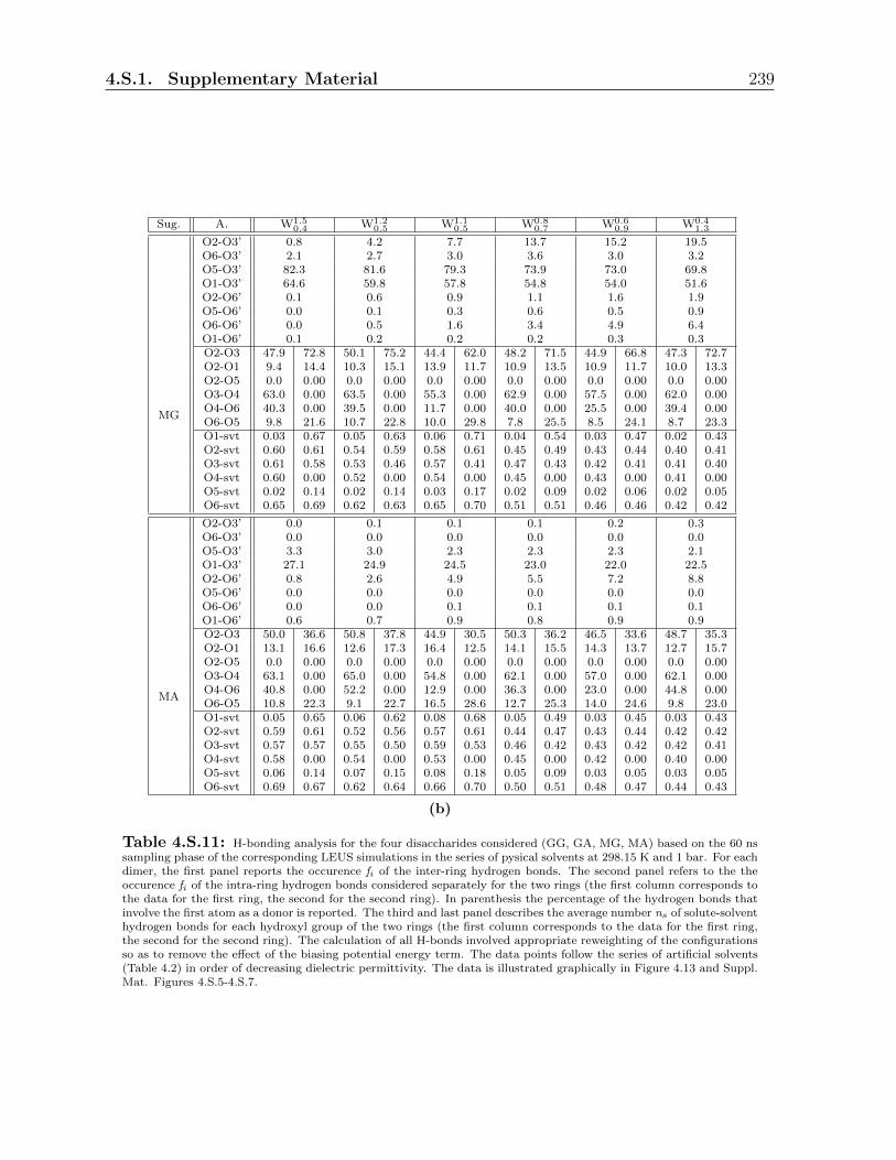
4.S.1. Supplementary Material 239
Sug. A. W1.50.4 W1.2
0.5 W1.10.5 W0.8
0.7 W0.60.9 W0.4
1.3
MG
O2-O3’ 0.8 4.2 7.7 13.7 15.2 19.5O6-O3’ 2.1 2.7 3.0 3.6 3.0 3.2O5-O3’ 82.3 81.6 79.3 73.9 73.0 69.8O1-O3’ 64.6 59.8 57.8 54.8 54.0 51.6O2-O6’ 0.1 0.6 0.9 1.1 1.6 1.9O5-O6’ 0.0 0.1 0.3 0.6 0.5 0.9O6-O6’ 0.0 0.5 1.6 3.4 4.9 6.4O1-O6’ 0.1 0.2 0.2 0.2 0.3 0.3O2-O3 47.9 72.8 50.1 75.2 44.4 62.0 48.2 71.5 44.9 66.8 47.3 72.7O2-O1 9.4 14.4 10.3 15.1 13.9 11.7 10.9 13.5 10.9 11.7 10.0 13.3O2-O5 0.0 0.00 0.0 0.00 0.0 0.00 0.0 0.00 0.0 0.00 0.0 0.00O3-O4 63.0 0.00 63.5 0.00 55.3 0.00 62.9 0.00 57.5 0.00 62.0 0.00O4-O6 40.3 0.00 39.5 0.00 11.7 0.00 40.0 0.00 25.5 0.00 39.4 0.00O6-O5 9.8 21.6 10.7 22.8 10.0 29.8 7.8 25.5 8.5 24.1 8.7 23.3O1-svt 0.03 0.67 0.05 0.63 0.06 0.71 0.04 0.54 0.03 0.47 0.02 0.43O2-svt 0.60 0.61 0.54 0.59 0.58 0.61 0.45 0.49 0.43 0.44 0.40 0.41O3-svt 0.61 0.58 0.53 0.46 0.57 0.41 0.47 0.43 0.42 0.41 0.41 0.40O4-svt 0.60 0.00 0.52 0.00 0.54 0.00 0.45 0.00 0.43 0.00 0.41 0.00O5-svt 0.02 0.14 0.02 0.14 0.03 0.17 0.02 0.09 0.02 0.06 0.02 0.05O6-svt 0.65 0.69 0.62 0.63 0.65 0.70 0.51 0.51 0.46 0.46 0.42 0.42
MA
O2-O3’ 0.0 0.1 0.1 0.1 0.2 0.3O6-O3’ 0.0 0.0 0.0 0.0 0.0 0.0O5-O3’ 3.3 3.0 2.3 2.3 2.3 2.1O1-O3’ 27.1 24.9 24.5 23.0 22.0 22.5O2-O6’ 0.8 2.6 4.9 5.5 7.2 8.8O5-O6’ 0.0 0.0 0.0 0.0 0.0 0.0O6-O6’ 0.0 0.0 0.1 0.1 0.1 0.1O1-O6’ 0.6 0.7 0.9 0.8 0.9 0.9O2-O3 50.0 36.6 50.8 37.8 44.9 30.5 50.3 36.2 46.5 33.6 48.7 35.3O2-O1 13.1 16.6 12.6 17.3 16.4 12.5 14.1 15.5 14.3 13.7 12.7 15.7O2-O5 0.0 0.00 0.0 0.00 0.0 0.00 0.0 0.00 0.0 0.00 0.0 0.00O3-O4 63.1 0.00 65.0 0.00 54.8 0.00 62.1 0.00 57.0 0.00 62.1 0.00O4-O6 40.8 0.00 52.2 0.00 12.9 0.00 36.3 0.00 23.0 0.00 44.8 0.00O6-O5 10.8 22.3 9.1 22.7 16.5 28.6 12.7 25.3 14.0 24.6 9.8 23.0O1-svt 0.05 0.65 0.06 0.62 0.08 0.68 0.05 0.49 0.03 0.45 0.03 0.43O2-svt 0.59 0.61 0.52 0.56 0.57 0.61 0.44 0.47 0.43 0.44 0.42 0.42O3-svt 0.57 0.57 0.55 0.50 0.59 0.53 0.46 0.42 0.43 0.42 0.42 0.41O4-svt 0.58 0.00 0.54 0.00 0.53 0.00 0.45 0.00 0.42 0.00 0.40 0.00O5-svt 0.06 0.14 0.07 0.15 0.08 0.18 0.05 0.09 0.03 0.05 0.03 0.05O6-svt 0.69 0.67 0.62 0.64 0.66 0.70 0.50 0.51 0.48 0.47 0.44 0.43
(b)
Table 4.S.11: H-bonding analysis for the four disaccharides considered (GG, GA, MG, MA) based on the 60 nssampling phase of the corresponding LEUS simulations in the series of pysical solvents at 298.15 K and 1 bar. For eachdimer, the first panel reports the occurence fi of the inter-ring hydrogen bonds. The second panel refers to the theoccurence fi of the intra-ring hydrogen bonds considered separately for the two rings (the first column corresponds tothe data for the first ring, the second for the second ring). In parenthesis the percentage of the hydrogen bonds thatinvolve the first atom as a donor is reported. The third and last panel describes the average number ns of solute-solventhydrogen bonds for each hydroxyl group of the two rings (the first column corresponds to the data for the first ring,the second for the second ring). The calculation of all H-bonds involved appropriate reweighting of the configurationsso as to remove the effect of the biasing potential energy term. The data points follow the series of artificial solvents(Table 4.2) in order of decreasing dielectric permittivity. The data is illustrated graphically in Figure 4.13 and Suppl.Mat. Figures 4.S.5-4.S.7.
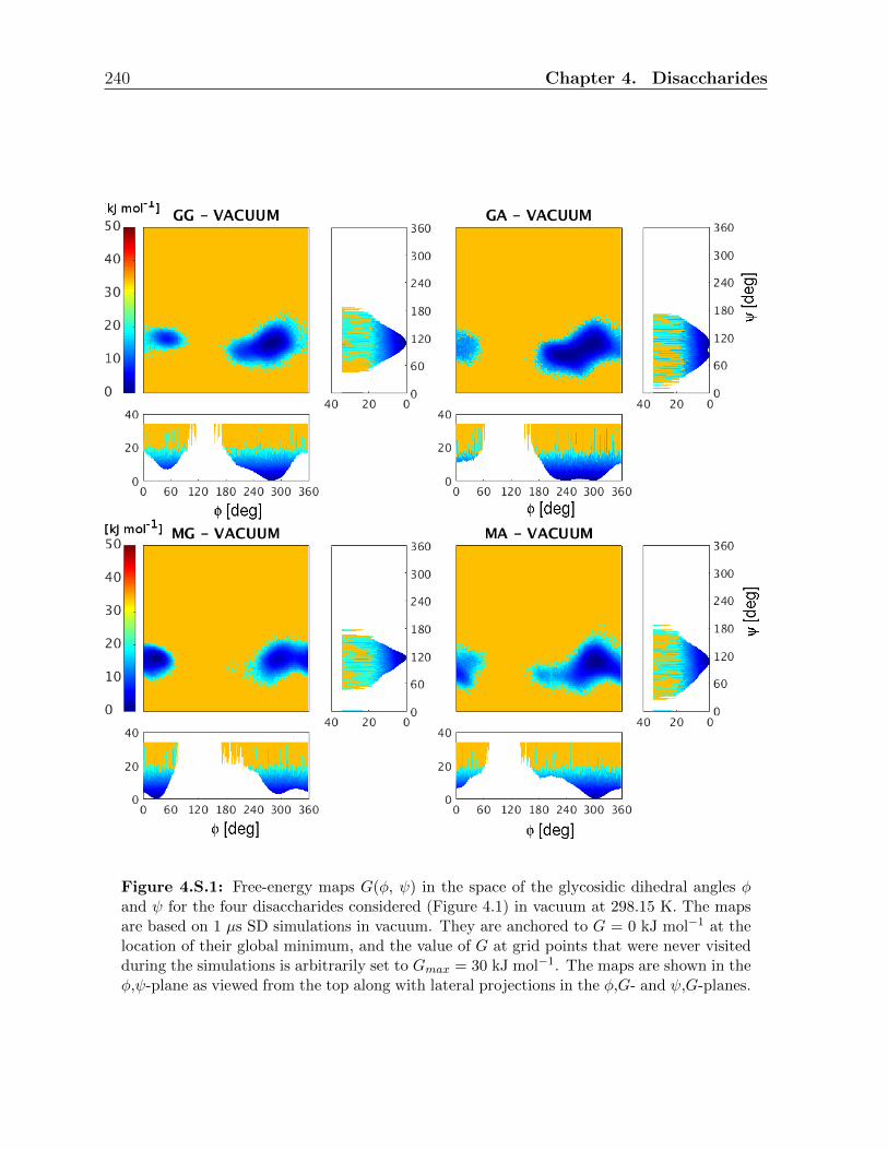
240 Chapter 4. Disaccharides
Figure 4.S.1: Free-energy maps G(φ, ψ) in the space of the glycosidic dihedral angles φand ψ for the four disaccharides considered (Figure 4.1) in vacuum at 298.15 K. The mapsare based on 1 µs SD simulations in vacuum. They are anchored to G = 0 kJ mol−1 at thelocation of their global minimum, and the value of G at grid points that were never visitedduring the simulations is arbitrarily set to Gmax = 30 kJ mol−1. The maps are shown in theφ,ψ-plane as viewed from the top along with lateral projections in the φ,G- and ψ,G-planes.

4.S.1. Supplementary Material 241
0.5
1
1.5
2
2.5
3
O1-
sug
H-bonding solute-solute (first ring)
0.5
1
1.5
2
2.5
3
O4-
sug
0.5
1
1.5
2
2.5
3
O2-
sug
0.5
1
1.5
2
2.5
3
O5-
sug
H2O DMSO CH
3OH CHCl
3CCl
4
0
0.5
1
1.5
2
2.5
3
O2-
sug
H2O DMSO CH
3OH CHCl
3CCl
4
0
0.5
1
1.5
2
2.5
3
O6-
sug
0.5
1
1.5
2
2.5
3
O1-
sug
GGGAMGMA
H-bonding solute-solute (second ring)
0.5
1
1.5
2
2.5
3
O4-
sug
0.5
1
1.5
2
2.5
3
O2-
sug
0.5
1
1.5
2
2.5
3
O5-
sug
H2O DMSO CH
3OH CHCl
3CCl
4
0
0.5
1
1.5
2
2.5
3
O3-
sug
H2O DMSO CH
3OH CHCl
3CCl
4
0
0.5
1
1.5
2
2.5
3
O6-
sug
0.51
1.52
2.5
3
O1-
svt
H-bonding solute-solvent (first ring)
0.511.522.5
3
O4-
svt
0.51
1.52
2.5
3
O2-
svt
0.511.522.5
3
O5-
svt
H2O DMSO CH
3OH CHCl
3CCl
4
00.5
11.5
22.5
3
O3-
svt
H2O DMSO CH
3OH CHCl
3CCl
4
00.511.522.5
3
O6-
svt
0.51
1.52
2.5
3
O1-
svt
H-bonding solute-solvent (second ring)
0.511.522.5
3
O4-
svt
0.51
1.52
2.5
3
O2-
svt
0.511.522.5
3
O5-
svt
H2O DMSO CH
3OH CHCl
3CCl
4
00.5
11.5
22.5
3
O3-
svt
H2O DMSO CH
3OH CHCl
3CCl
4
00.511.522.5
3
O6-
svt
Figure 4.S.2: Numbers of H-bonds involving specific solute atoms for the four disaccharidesconsidered in the physical solvents at 298.15 K and 1 bar. The results are based on the60 ns sampling phases of the corresponding LEUS simulations. In the top panels, the totalaverage number ni of solute-solute H-bonds is reported separately for each hydroxyl groupof the two rings. In the bottom panels, the average number ns of solute-solvent H-bondsis reported separately for each hydroxyl group of the two rings. All the hydroxyl groupsin the two rings were considered for the analysis. The figure does not distinguish betweendonors and acceptors. The calculation of H-bonds involved appropriate reweighting of theconfigurations so as to remove the effect of the biasing potential energy term. The graphson left side describe H-bonds involving the atoms the first ring, while those on the right sidedescribe the H-bonds involving the atoms of the second ring. The data points follow theseries of physical solvents (Table 4.1) in order of decreasing polarity. The different colorsrefer to the four disaccharides (Figure 4.1), namely GG, MG, GA, MA. The data is reportednumerically in Suppl. Mat. Table 4.S.3.

242 Chapter 4. Disaccharides
20406080
100
O2-
O3’
GGGAMGMA
H-bonding Interresidue
20406080100
O2-
O6’
012345
O6-
O3’
12345
O5-
O6’
H2O DMSO CH
3OH CHCl
3CCl
4
020406080
100
O5-
O3’
H2O DMSO CH
3OH CHCl
3CCl
4
5
10
15
20
O6-
O6’
Figure 4.S.3: Occurrences (in percent) of interresidue H-bonds for the four disacchar-ides considered in the series of physical solvents at 298.15 K and 1 bar. The results arebased on the 60 ns sampling phases of the corresponding LEUS simulations. All pairs ofhydroxyl groups involving the two rings were considered for the analysis, but only H-bondswith occurrences of at least 0.1 % are reported. The figure does not distinguish betweendonors and acceptors. The calculation of H-bonds involved appropriate reweighting of theconfigurations so as to remove the effect of the biasing potential energy term. The panelson the left side describe H-bonds involving the atoms HO′3 and O′3 of the second ring, whilethose on the right side describe the H-bonds involving the atoms HO′6 and O′6. The datapoints follow the series of physical solvents (Table 4.1) in order of decreasing polarity. Thedifferent colors refer to the four disaccharides (Figure 4.1), namely GG, MG, GA, MA. Thedata is reported numerically in Suppl. Mat. Table 4.S.3.

4.S.1. Supplementary Material 243
020406080100
O2-O3
H-b
ondi
ng
intr
ares
idue
(fi
rst r
ing)
20406080100
O3-O4
01020304050
O2-O1
20406080100
O4-O6
H2O
DM
SOC
H3O
HC
HC
l 3C
Cl 4
01020304050
O2-O5
H2O
DM
SOC
H3O
HC
HC
l 3C
Cl 4
01020304050
O6-O5
020406080100
O2-O3
GG
GA
MG
MA
H
-bon
ding
i
ntra
resi
due
(sec
ond
ring
)
20406080100
O3-O4
01020304050
O2-O1
20406080100
O4-O6
H2O
DM
SOC
H3O
HC
HC
l 3C
Cl 4
020406080100
O2-O5
H2O
DM
SOC
H3O
HC
HC
l 3C
Cl 4
01020304050
O6-O5
Figure
4.S.4:
Occ
urr
ence
s(i
np
erce
nt)
ofin
trar
esid
ue
H-b
ond
sfo
rth
efo
ur
dis
acch
ari
des
con
sid
ered
inth
ese
ries
ofp
hysi
cal
solv
ents
at29
8.15
Kan
d1
bar
.T
he
resu
lts
base
don
the
60n
ssa
mp
lin
gp
hase
sof
the
corr
esp
ond
ing
LE
US
sim
ula
tion
s.A
llth
ehyd
roxyl
gro
up
sin
the
two
rin
gs
wer
eco
nsi
der
edfo
rth
ean
alysi
s,b
ut
only
H-b
ond
sw
ith
occ
urr
ence
sof
at
least
0.1
%are
rep
ort
ed.
Th
efi
gure
does
not
dis
tin
guis
hb
etw
een
don
ors
and
acc
epto
rs.
Th
eca
lcu
lati
onof
H-b
on
ds
invo
lved
app
rop
riat
ere
wei
ghti
ng
ofth
eco
nfi
gura
tion
sso
as
tore
mov
eth
eeff
ect
of
the
bia
sing
pot
enti
alen
ergy
term
.T
he
grap
hs
onle
ftsi
de
des
crib
eH
-b
on
ds
invo
lvin
gth
eato
ms
the
firs
tri
ng,
wh
ile
thos
eon
the
righ
tsi
de
des
crib
eth
ehyd
rogen
bon
ds
invo
lvin
gth
eato
ms
ofth
ese
con
dri
ng.
Th
ed
ata
poi
nts
foll
owth
ese
ries
of
physi
cal
solv
ents
(Tab
le4.1
)in
ord
erof
dec
reas
ing
pol
arit
y.T
he
diff
eren
tco
lors
refe
rto
the
fou
rd
isacc
har
ides
(Fig
ure
4.1
),n
amel
yG
G,
MG
,G
A,
MA
.T
he
dat
ais
rep
orte
dnu
mer
icall
yin
Su
pp
l.M
at.
Tab
le4.
S.3
.

244 Chapter 4. Disaccharides
2
4
6
O2-
O3’
GGGAMGMA
H-bonding Interresidue
5
10
15
20
O2-
O6’
0
2
4
6
O6-
O3’
2
4
6
O5-
O6’
020406080
100
O5-
O3’
2
4
6
O6-
O6’
W0.8
1.4W
0.9
1.2W
1.0
1.0 W1.5
0.5
020406080
100
O1-
O3’
W0.8
1.4W
0.9
1.2W
1.0
1.0 W1.5
0.5
0
2
4
6
O1-
O6’
20406080
100
O2-
O3’
H-bonding Interresidue
20406080100
O2-
O6’
0
2
4
6
O6-
O3’
2
4
6
O5-
O6’
020406080
100
O5-
O3’
5
10
15
20
O6-
O6’
W0.5
1.4W
0.8
0.9W
0.7
0.6 W0.5
0.3
020406080
100
O1-
O3’
W0.5
1.4W
0.8
0.9W
0.7
0.6 W0.5
0.3
0
5
10
15
20
O1-
O6’
2
4
6
O2-
O3’
H-bonding Interresidue
5
10
15
20
O2-
O6’
0
2
4
6
O6-
O3’
2
4
6
O5-
O6’
020406080
100
O5-
O3’
2
4
6
O6-
O6’
W1.1
0.9W
1.0
1.0W
0.8
1.1W
0.7
1.2 W0.6
1.4W
0.5
1.5
020406080
100
O1-
O3’
W1.1
0.9W
1.0
1.0W
0.8
1.1W
0.7
1.2 W0.6
1.4W
0.5
1.5
0
2
4
6
O1-
O6’
20406080
100
O2-
O3’
H-bonding Interresidue
20406080100
O2-
O6’
0
2
4
6
O6-
O3’
2
4
6
O5-
O6’
020406080
100
O5-
O3’
5
10
15
20
O6-
O6’
W1.5
0.4W
1.2
0.5W
1.1
0.5W
0.8
0.7 W0.6
0.9W
0.4
1.3W
0.9
0.6
20
40
60
80
100
O1-
O3’
W1.5
0.4W
1.2
0.5W
1.1
0.5W
0.8
0.7 W0.6
0.9W
0.4
1.3W
0.9
0.6
0
5
10
15
20
O1-
O6’
Figure 4.S.5: Occurrences (in percent) of interresidue H-bonds for the four disaccharidesconsidered in the series of artificial solvents at 298.15 K and 968 kg·m−3. The results arebased on the 60 ns sampling phases of the corresponding LEUS simulations. All pairs ofhydroxyl groups involving the two rings were considered for the analysis, but only H-bondswith occurrences of at least 0.1 % are reported. The figure does not distinguish betweendonors and acceptors. The calculation of H-bonds involved appropriate reweighting of theconfigurations so as to remove the effect of the biasing potential energy term. The grphson the left side describe H-bonds involving the atoms HO′3 and O′3 of the second ring,while those on the right side describe the H-bonds involving the atoms HO′6 and O′6. Thedata points follow the series of artificial solvents (Table 4.2): in the top graphs the seriesconsidered are the SHp (on the left) and the Shp (on the right) in order of decreasing dielectric
permittivity; in the bottom graphs the series considered are the SPh (on the left) and the Sph(on the right) in order of decreasing H-bonding capacity. The different colors refer to thefour disaccharides (Figure 4.1), namely GG, MG, GA, MA. The data is reported numericallyin Suppl. Mat. Tables 4.S.8, 4.S.9, 4.S.10 and 4.S.11.

4.S.1. Supplementary Material 245
020406080100
O2-O3
H
-bon
ding
I
ntra
resi
due
(fir
st r
ing)
20406080100
O3-O4
102030
02-O1
102030
O4-O6
W0.
8
1.4
W0.
9
1.2
W1.
0
1.0
W1.
5
0.5
0102030
O2-O5
W0.
8
1.4
W0.
9
1.2
W1.
0
1.0
W1.
5
0.5
0102030
O6-O5
020406080100
O2-O3
H
-bon
ding
I
ntra
resi
due
(fir
st r
ing)
20406080100
O3-O4
0102030
O2-O1
20406080100
O4-O6
W0.
5
1.4
W0.
8
0.9
W0.
7
0.6
W0.
5
0.3
0102030
O2-O5
W0.
5
1.4
W0.
8
0.9
W0.
7
0.6
W0.
5
0.3
0102030
O6-O5
020406080100
O2-O3
H
-bon
ding
I
ntra
resi
due
(fir
st r
ing)
20406080100
O3-O4
0102030
O2-O1
102030O4-O6
W0.
9
1.1
W1.
0
1.0
W0.
8
1.1
W0.
7
1.2
W0.
6
1.4
W0.
5
1.5
0102030
O2-O5
W0.
9
1.1
W1.
0
1.0
W0.
8
1.1
W0.
7
1.2
W0.
6
1.4
W0.
5
1.5
0102030
O6-O5020406080100
O2-O3
H
-bon
ding
I
ntra
resi
due
(fir
st r
ing)
20406080100
O3-O4
0102030
O2-O1
20406080100
O4-O6
W1.
5
0.4
W1.
2
0.5
W1.
1
0.5
W0.
8
0.7
W0.
6
0.9
W0.
4
1.3
W0.
9
0.6
0102030
O2-O5
W1.
5
0.4
W1.
2
0.5
W1.
1
0.5
W0.
8
0.7
W0.
6
0.9
W0.
4
1.3
W0.
9
0.6
0102030
O6-O5
020406080100
O2-O3
H
-bon
ding
I
ntra
resi
due
(sec
ond
ring
)
020406080100
O3-O4
1020304050
O2-O1
020406080100
O4-O6
W0.
5
1.4
W0.
8
0.9
W0.
7
0.6
W0.
5
0.3
020406080100
O2-O5
W0.
5
1.4
W0.
8
0.9
W0.
7
0.6
W0.
5
0.3
01020304050
O6-O5
020406080100
O2-O3
GG
GA
MG
MA
H
-bon
ding
I
ntra
resi
due
(sec
ond
ring
)
020406080100
O3-O4
01020304050
O2-O1
020406080100
O4-O6
W0.
5
1.4
W0.
8
0.9
W0.
7
0.6
W0.
5
0.3
020406080100
O2-O5
W0.
5
1.4
W0.
8
0.9
W0.
7
0.6
W0.
5
0.3
1020304050
O6-O5
020406080100
O2-O3
H
-bon
ding
I
ntra
resi
due
(sec
ond
ring
)
020406080100
O3-O4
01020304050
O2-O1
020406080100
O4-O6
W0.
9
1.1
W1.
0
1.0
W0.
8
1.1
W0.
7
1.2
W0.
6
1.4
W0.
5
1.5
020406080100
O2-O5
W0.
9
1.1
W1.
0
1.0
W0.
8
1.1
W0.
7
1.2
W0.
6
1.4
W0.
5
1.5
1020304050
O6-O5
020406080100
O2-O3
H
-bon
ding
I
ntra
resi
due
(sec
ond
ring
)
020406080100
O3-O4
1020304050
O2-O1
020406080100
O4-O6
W1.
5
0.4
W1.
2
0.5
W1.
1
0.5
W0.
8
0.7
W0.
6
0.9
W0.
4
1.3
W0.
9
0.6
020406080100
O2-O5
W1.
5
0.4
W1.
2
0.5
W1.
1
0.5
W0.
8
0.7
W0.
6
0.9
W0.
4
1.3
W0.
9
0.6
1020304050
O6-O5
Figure
4.S.6:
Occ
urr
ence
s(i
np
erce
nt)
ofin
trar
esid
ue
H-b
ond
sfo
rth
efo
ur
dis
acc
hari
des
con
sid
ered
inth
ese
ries
ofar
tifi
cial
solv
ents
at29
8.15
Kan
d96
8kg·
m−
3.
Th
ere
sult
sb
ase
don
the
60
ns
sam
pli
ng
ph
ases
ofth
eco
rres
pon
din
gL
EU
Ssi
mu
lati
ons.
All
the
hyd
roxyl
grou
ps
inth
etw
ori
ngs
wer
eco
nsi
der
edfo
rth
ean
alysi
s,b
ut
only
H-b
ond
sw
ith
occ
urr
ence
sof
at
leas
t0.1
%are
rep
orte
d.
Th
efi
gure
does
not
dis
tin
guis
hb
etw
een
don
ors
an
dacc
epto
rs.
Th
eca
lcu
lati
on
of
H-b
ond
sin
volv
edap
pro
pri
ate
rew
eigh
tin
gof
the
con
figu
rati
on
sso
as
tore
mov
eth
eeff
ect
ofth
eb
iasi
ng
pot
enti
alen
ergy
term
.T
he
grap
hon
left
side
des
crib
esH
-b
ond
sin
volv
ing
the
atom
sth
efi
rst
rin
g,w
hil
eth
ose
onth
eri
ght
sid
ed
escr
ibe
the
hyd
rogen
bon
ds
invo
lvin
gth
eato
ms
ofth
ese
con
dri
ng.
Th
ed
ata
poi
nts
foll
owth
ese
ries
of
art
ifici
al
solv
ents
(Tab
le4.
2):
inth
eto
pgr
aph
sth
ese
ries
con
sid
ered
are
theSH p
(on
the
left
)an
d
theSh p
(on
the
righ
t)in
ord
erof
dec
reas
ing
die
lect
ric
per
mit
tivit
y;
inth
eb
otto
mgra
ph
sth
e
seri
esco
nsi
der
edare
theSP h
(on
the
left
)an
dth
eSp h
(on
the
righ
t)in
order
ofd
ecre
asi
ng
H-b
ond
ing
cap
aci
ty.
Th
ed
iffer
ent
colo
rsre
fer
toth
efo
ur
dis
acch
arid
es(F
igu
re4.1
),n
am
ely
GG
,M
G,
GA
,M
A.
Th
ed
ata
isre
por
ted
nu
mer
ical
lyin
Su
pp
l.M
at.
Tab
les
4.S
.8,
4.S
.9,
4.S
.10
and
4.S
.11.

246 Chapter 4. Disaccharides
0.51
1.52
2.53
O1-svt
H
-bon
ding
s
olut
e-so
lven
t (fi
rst r
ing)
0.5
11.5
22.5
3
O4-svt
0.51
1.52
2.53
O2-svt
0.5
11.5
22.5
3
O5-svt
W0.
8
1.4
W0.
9
1.2
W1.
0
1.0
W1.
5
0.5
00.
511.
522.
53
O3-svt
W0.
8
1.4
W0.
9
1.2
W1.
0
1.0
W1.
5
0.5
00.5
11.5
22.5
3
O6-svt
0.2
0.4
0.6
0.81
O1-svt
H
-bon
ding
s
olut
e-so
lven
t (fi
rst r
ing)
0.2
0.4
0.6
0.8
1
O4-svt
0.2
0.4
0.6
0.81
O2-svt
0.2
0.4
0.6
0.8
1
O5-svt
W0.
5
1.4
W0.
8
0.9
W0.
7
0.6
W0.
5
0.3
0
0.2
0.4
0.6
0.81
O3-svt
W0.
5
1.4
W0.
8
0.9
W0.
7
0.6
W0.
5
0.3
00.2
0.4
0.6
0.8
1
O6-svt
0.51
1.52
2.53
O1-svt
H
-bon
ding
s
olut
e-so
lven
t (fi
rst r
ing)
0.5
11.5
22.5
3
O4-svt
0.51
1.52
2.53
O2-svt
0.5
11.5
22.5
3O5-svt
W0.
9
1.1
W1.
0
1.0
W0.
8
1.1
W0.
7
1.2
W0.
6
1.4
W0.
5
1.5
00.
511.
522.
53
O3-svt
W0.
9
1.1
W1.
0
1.0
W0.
8
1.1
W0.
7
1.2
W0.
6
1.4
W0.
5
1.5
00.5
11.5
22.5
3
O6-svt0.
2
0.4
0.6
0.81
O1-svt
H
-bon
ding
s
olut
e-so
lven
t (fi
rst r
ing)
0.2
0.4
0.6
0.8
1
O4-svt
0.2
0.4
0.6
0.81
O2-svt
0.2
0.4
0.6
0.8
1
O5-svt
W1.
5
0.4
W1.
2
0.5
W1.
1
0.5
W0.
8
0.7
W0.
6
0.9
W0.
4
1.3
W0.
9
0.6
0.2
0.4
0.6
0.81
O3-svt
W1.
5
0.4
W1.
2
0.5
W1.
1
0.5
W0.
8
0.7
W0.
6
0.9
W0.
4
1.3
W0.
9
0.6
0.2
0.4
0.6
0.8
1
O6-svt
0.51
1.52
2.53
O1-svt
H
-bon
ding
s
olut
e-so
lven
t (fi
rst r
ing)
0.5
11.5
22.5
3
O4-svt
0.51
1.52
2.53
O2-svt
0.5
11.5
22.5
3
O5-svt
W0.
8
1.4
W0.
9
1.2
W1.
0
1.0
W1.
5
0.5
0.51
1.52
2.53
O3-svt
W0.
8
1.4
W0.
9
1.2
W1.
0
1.0
W1.
5
0.5
00.5
11.5
22.5
3
O6-svt
0.2
0.4
0.6
0.81
O1-svt
GG
GA
MG
MA
H
-bon
ding
s
olut
e-so
lven
t (se
cond
rin
g)
0.2
0.4
0.6
0.8
1
O4-svt
0.2
0.4
0.6
0.81
O2-svt
0.2
0.4
0.6
0.8
1
O5-svt
W0.
5
1.4
W0.
8
0.9
W0.
7
0.6
W0.
5
0.3
0
0.2
0.4
0.6
0.81
O3-svt
W0.
5
1.4
W0.
8
0.9
W0.
7
0.6
W0.
5
0.3
00.2
0.4
0.6
0.8
1
O6-svt
0.51
1.52
2.53
O1-svt
H
-bon
ding
s
olut
e-so
lven
t (se
cond
rin
g)
0.5
11.5
22.5
3
O4-svt
0.51
1.52
2.53
O2-svt
0.5
11.5
22.5
3
O5-svt
W0.
9
1.1
W1.
0
1.0
W0.
8
1.1
W0.
7
1.2
W0.
6
1.4
W0.
5
1.5
00.
511.
522.
53
O3-svt
W0.
9
1.1
W1.
0
1.0
W0.
8
1.1
W0.
7
1.2
W0.
6
1.4
W0.
5
1.5
00.5
11.5
22.5
3
O6-svt
0.2
0.4
0.6
0.81
O1-svt
H
-bon
ding
s
olut
e-so
lven
t (se
cond
rin
g)
0.2
0.4
0.6
0.8
1
O4-svt
0.2
0.4
0.6
0.81
O2-svt
0.2
0.4
0.6
0.8
1
O5-svt
W1.
5
0.4
W1.
2
0.5
W1.
1
0.5
W0.
8
0.7
W0.
6
0.9
W0.
4
1.3
W0.
9
0.6
0
0.2
0.4
0.6
0.81
O3-svt
W1.
5
0.4
W1.
2
0.5
W1.
1
0.5
W0.
8
0.7
W0.
6
0.9
W0.
4
1.3
W0.
9
0.6
00.2
0.4
0.6
0.8
1
O6-svt
Figure
4.S.7:
Nu
mb
ers
ofso
lute
-sol
vent
H-b
ond
sin
volv
ing
spec
ific
solu
teato
ms
for
the
fou
rd
isac
char
ides
con
sid
ered
inth
ear
tifi
cial
solv
ents
at29
8.15
Kan
d96
8kg·m−
3.
Th
ere
sult
sar
eb
ased
on
the
60n
ssa
mp
lin
gp
has
esof
the
corr
esp
ond
ing
LE
US
sim
ula
tion
s.T
he
aver
age
nu
mb
erns
of
solu
te-s
olve
nt
H-b
ond
sis
rep
orte
dse
par
atel
yfo
rth
etw
ori
ngs.
All
the
hyd
roxyl
grou
ps
inth
etw
ori
ngs
wer
eco
nsi
der
edfo
rth
ean
alysi
s.T
he
figu
red
oes
not
dis
tin
guis
hb
etw
een
don
ors
and
acce
pto
rs.
Th
eca
lcu
lati
onof
H-b
ond
sin
volv
edap
pro
pri
ate
rew
eigh
tin
gof
the
con
figu
rati
ons
soas
tore
mov
eth
eeff
ect
ofth
eb
iasi
ng
pot
enti
al
ener
gy
term
.T
he
grap
hs
onle
ftsi
de
des
crib
esH
-bon
ds
invo
lvin
gth
eat
oms
the
firs
tri
ng,
wh
ile
thos
eon
the
righ
tsi
de
des
crib
eth
eH
-bon
ds
invo
lvin
gth
eat
oms
ofth
ese
con
dri
ng.
Th
ed
ata
poin
tsfo
llow
the
seri
esof
arti
fici
also
lven
ts(T
able
4.2)
:in
the
top
gra
ph
sth
ese
ries
con
sid
ered
are
theSH p
(on
the
left
)an
dth
eSh p
(on
the
righ
t)in
ord
erof
dec
reas
ing
die
lect
ric
per
mit
tivit
y;
inth
eb
ott
omgr
aph
sth
ese
ries
con
sid
ered
are
theSP h
(on
the
left
)an
dth
eSp h
(on
the
right)
inord
erof
dec
reas
ing
H-b
ond
ing
cap
acit
y.T
he
diff
eren
tco
lors
refe
rto
the
fou
rd
isac
chari
des
(Fig
ure
4.1)
,nam
ely
GG
,M
G,G
A,M
A.T
he
dat
ais
rep
ort
ednu
mer
icall
yin
Su
pp
l.M
at.
Tab
les
4.S
.8,
4.S
.9,
4.S
.10
and
4.S
.11.

Chapter 5
Outlook
Molecular dynamics simulation is becoming an ever more important tool in the study
of molecular systems. With the steady increase in the power of computers, the system
dimension and time-scales that are accessible for computer simulations have reached a
regime relevant for experimentally studied (bio)chemical processes. The reproduction
of physically realistic conditions is not the only aspect of simulations. Artificial and
unphysical situations are important alternatives.
In Chapter 2 artificial solvent models derived from the simple point charges water model
by systematic modification of the oxygen-hydrogen bond length and of the atomic partial
charges were developed. The consequences of the variation of these two parameters on
the collective properties of the liquid can give insights into the particular nature of this
fundamental solvent. In this chapter the focus was on the basic properties of the liquid
and particular attention was given to the dielectric permittivity and hydrogen-bonding ca-
pacity, as these properties are strongly connected to the polarity of the solvent. Additional
properties might be calculated to obtain a more complete characterization, e.g. viscosity,
surface tension, heat capacity, thermal expansion coefficient or isothermal compressibility.
It would also be interesting to correlate these properties with the dipole moment of the
models, as well as with their higher order multipole moments. Moreover, the same ap-
proach might be used to systematically vary other parameters related to the geometry of
the water molecule (e.g. the bond angle).
From an application point of view, these models can help in the study of the solvent
247

248 Chapter 5. Outlook
effects on solute molecule, as done in Chapter 3 and Chapter 4. They allow to disentangle
the effects of the dielectric permittivity and of the H-bonding capacity of the solvent, while
keeping its molecular size and shape constant, as well as water-like dispersive interactions.
All kind of solute molecules experiencing conformational changes in non-aqueous environ-
ments might be simulated in these artificial solvents, and their behaviour as function of
the solvent polarity analyzed.
Carbohydrates are a particularly fascinating type of molecules, and their variety and
flexibility make them an endless source of study material. In Chapter 3 and Chapter 4,
the importance of intramolecular hydrogen-bonding for these molecules was investigated
in physical solvents of different polarity, as well as in the artificial solvents developed in
Chapter 2. Hydrogen-bonding is often regarded as a fundamental driving force for the
conformational properties of (bio)polymers. In our study, in aqueous environment, it was
found to be an opportunistic consequence of the close proximity of two H-bonding groups
in a given conformation, and not a factor contributing to the stability of this conforma-
tion. This is true for both monosaccharides and disaccharides. On the other hand, with
a decrease of the solvent polarity, solvent-exposed hydrogen-bonding progressively evolves
from a negligible to a very significant conformational steering force. However, introdu-
cing additional degrees of freedom that increase the complexity of the molecules (from
monomers to dimers), the importance of intramolecular hydrogen-bonding in low polarity
solvents takes a different form. Possible competition between hydrogen-bonds that mutu-
ally exclude each others can tune their influence, making them an adverse factor towards
specific conformational preferences.
A generalization of this behaviour, especially in case of disaccharides, would be inter-
esting. A more systematic study on different glycosidic linkages might help to understand
what is so determinant for the conformational properties of carbohydrates in the aqueous
environment. As hydrogen-bonding is generally considered a significant stabilizing factor

249
for the secondary structure of long carbohydrate chains, it would also be interesting to
consider longer polymers. Alternative toy-systems might be used for a better understand-
ing of hydrogen-bond competition. Furthermore, in view of these considerations about
carbohydrates, a general rethinking about the role of hydrogen-bonding for (bio)polymers
in aqueous environment would be necessary.


Bibliography
[1] N. Bohr, On the constitution of atoms and molecule, Philos. Mag. 26 (1913), pp. 1-24.
[2] N. Metropolis, A.W. Rosenbluth, M.N. Rosenbluth, A.H. Teller and E. Teller, Equation of state calculations by fastcomputing machines, J. Chem. Phys. 21 (1953), pp. 1087-1092.
[3] M.P. Allen and D.J. Tildesley, Computer simulation of liquids, Oxford University Press, New York, USA (1987).
[4] W.F. van Gunsteren and H.J.C. Berendsen, Computer simulation of molecular dynamics: Methodology, applicationsand perspectives in chemistry, Angew. Chem. Int. Ed. 29 (1990), pp. 992-1023.
[5] W.F. van Gunsteren, D. Bakowies, R. Baron, I Chandrasekhar, M. Christen, X. Daura, P. Gee, D.P. Geerke, A.Glattli, P.H. Hunenberger, M.A. Kastenholz, C. Oostenbrink, M. Schenk, D. Trzesniak, N.F.A. van der Vegt and H.B.Yu, Biomolecular modelling: goals, problems, perspectives, Angew. Chem. Int. Ed. 45 (2006), pp. 4064-4092.
[6] H.J.C. Berendsen, Simulating the physical world, Cambridge University Press, Cambridge, UK (2007).
[7] C.Y. Wang and X. Zhang, Multiscale modeling and related hybrid approaches, Curr. Opin. Solid State Mat. Sci. 10(2006), pp. 2-14.
[8] M. Praprotnik, L. Delle Site and K. Kremer, Multiscale simulation of soft matter: From scale bridging to adaptiveresolution, Ann. Rev. Phys. Chem. 59 (2008), pp. 545-571.
[9] P.H. Hunenberger and W.F. van Gunsteren Empirical classical interaction functions for molecular simulations In: Com-puter simulation of biomolecular systems, theoretical and experimental applications Volume 3.; W.F. van Gunsteren,P.K. Weiner and A.J. Wilkinson, Eds.; Kluwer/Escom Science Publishers, Dordrecht, The Netherlands (1997); pp3-82..
[10] D. Frenkel and B. Smit, Understanding molecular simulation Edition 2., Academic Press, San Diego, USA (2002).
[11] W.F. van Gunsteren, T. Huber and A.E. Torda, Biomolecular modelling: overview of types of methods to search andsample conformational space, AIP Conf. Proc. 330 (1995), pp. 253-268.
[12] A.F. Voter, F. Monatlenti and T.C. Germann, Extending the time scale in atomistic simulations of materials, Annu.Rev. Mater. Res. 32 (2002), pp. 321-46.
[13] M. Christen and W.F. van Gunsteren, On searching in, sampling of, and dynamically moving through conformationalspace of biomolecular systems: A review, J. Comput. Chem. 29 (2008), pp. 157-166.
[14] H.S. Hansen and P.H. Hunenberger, Using the local elevation method to construct optimized umbrella sampling po-tentials: Calculation of the relative free energies and interconversion barriers of glucopyranose ring conformers inwater, J. Comput. Chem. 31 (2010), pp. 1-23.
[15] H.S. Hansen and P.H. Hunenberger, Ball-and-stick local elevation umbrella sampling: molecular simulations involvingenhanced sampling within conformational or alchemical subspaces of low internal dimensionalities, minimal irrelevantvolume and problem-adapted geometries, J. Chem. Theory Comput. 6 (2010), pp. 2622-2646.
[16] P.H. Hunenberger, Thermostat algorithms for molecular dynamics simulations, Adv. Polym. Sci. 173 (2005), pp.105-149.
[17] W.F. van Gunsteren and M. Karplus, Effect of constraints, solvent and crystal environment on protein dynamics,Nature 293 (1981), pp. 677-678.
[18] J. Warwicker and H.C. Watson, Calculation of the electric potential in the active site cleft due to α-helix dipoles, J.Mol. Biol. 157 (1982), pp. 671-679.
[19] M.K. Gilson and B. Honig, Calculation of the total electrostatic energy of a macromolecular system: solvation energies,binding energies, and conformational analysis, Proteins: Struct. Funct. Genet. 4 (1988), pp. 7-18.
[20] S.C. Harvey, Treatment of electrostatic effects in macromolecular modeling, Proteins: Struct. Funct. Genet. 5 (1989),pp. 78-92.
[21] M.E. Davis and J.A. McCammon, Electrostatics in biomolecular structure and dynamics, Chem. Rev. 90 (1990), pp.509-521.
251
252 BIBLIOGRAPHY
[22] J.D. Madura, M.E. Davis, M.K. Gilson, R.C. Wade, B.A. Luty and J.A. McCammon Biological applications ofelectrostatic calculations and Brownian dynamics simulations In: Reviews in computational chemistry Volume 4.;K.B. Lipkowitz and D.B. Boyd, Eds.; VCH Publishers Inc., New York, USA (1994); pp 229-267.
[23] B. Honig and A. Nicholls, Classical electrostatics in biology and chemistry, Science 268 (1995), pp. 1144-1149.
[24] A. Warshel and A. Papazyan, Electrostatic effects in macromolecules: Fundamental concepts and practical modeling,Curr. Opin. Struct. Biol. 8 (1998), pp. 211-217.
[25] B. Roux and T. Simonson, Implicit solvent models, Biophys. Chem. 78 (1999), pp. 1-20.
[26] N.A. Baker, Improving implicit solvent simulations: a Poisson-centric view, Curr. Opin. Struct. Biol. 15 (2005), pp.137-143.
[27] J.H. Chen, C.L. Brooks and J. Khandogin, Recent advances in implicit solvent-based methods for biomolecular sim-ulations, Curr. Opin. Struct. Biol. 18 (2008), pp. 140-148.
[28] M. Levitt and A. Warshel, Computer simulation of protein folding, Nature 253 (1975), pp. 694-698.
[29] B. Smit, P.A.J. Hilbers, K. Esselink, L.A.M. Rupert, N.M. van Os and A.G. Schlijper, Computer simulations of awater/oil interface in the presence of micelles, Nature 348 (1990), pp. 624-625.
[30] M.L. Huertas, S. Navarro, M.C.L. Martinez and J.G. de la Torre, Simulation of the conformation and dynamics of adouble-helical model for DNA, Biophys. J. 73 (1997), pp. 3142-3153.
[31] R.L.C. Akkermans and W.J. Briels, Coarse-grained dynamics of one chain in a polymer melt, J. Chem. Phys. 113(2000), pp. 6409-6422.
[32] J. Baschnagel, K. Binder, P. Doruker, A.A. Gusev, O. Hahn, K. Kremer, W.L. Mattice, F. Muller-Plathe, M. Murat,W. Paul, S. Santos, U.W. Suter and W. Tries, Bridging the gap between atomistic and coarse-grained models ofpolymers: status and perspectives, Adv. Polym. Sci. 152 (2000), pp. 41-156.
[33] K. Drukker, G. Wu and G.C. Schatz, Model simulations of DNA denaturation dynamic, J. Chem. Phys. 114 (2001),pp. 579-590.
[34] F. Muller-Plathe, Coarse-graining in polymer simulations: From the atomistic to the mesoscopic scale and back,Chem. Phys. Chem. 3 (2002), pp. 754-769.
[35] S.J. Marrink, A.H. de Vries and A.E. Mark, Coarse grained model for semiquantitative lipid simulations, J. Phys.Chem B 108 (2004), pp. 750-760.
[36] V. Molinero and W.A. Goddard III, M3B: A coarse-grained force field for molecular simulations of malto-oligosaccharides and their water mixtures, J. Phys. Chem. B 108 (2004), pp. 1414-1427.
[37] S.O. Nielsen, C.F. Lopez, G. Srinivas and M.L. Klein, Coarse grain models and the computer simulation of softmaterials, J. Phys.: Condens. Matter 16 (2004), pp. R481-R512.
[38] A. van den Noort, W.K. den Otter and W.J. Briels, Coarse graining of slow variables in dynamic simulations of softmatter, Europhys. Lett. 80 (2007), pp. 28003/1-28003/5.
[39] G.A. Voth, Coarse-graining of condensed phase and biomolecular systems, Taylor & Francis, Inc., New York, USA(2008).
[40] A. Warshel and M. Levitt, Theoretical studies of enzymic reactions - dielectric, electrostatic and steric stabilizationof carbonium-ion in reaction of lysozyme, J. Mol. Biol. 103 (1976), pp. 227-249.
[41] W.L. Jorgensen and J. Tirado-Rives, The OPLS potential functions for proteins. Energy minimizations for crystalsof cyclic peptides and crambin, J. Am. Chem. Soc. 110 (1988), pp. 1657-1666.
[42] W.L. Jorgensen, D.S. Maxwell and J. Tirado-Rives, Development and testing of the OPLS all-atom force field onconformational energetics and properties of organic liquids, J. Am. Chem. Soc. 118 (1996), pp. 11225-11236.
[43] P.K. Weiner and P.A. Kollman, AMBER - Assisted model building with energy refinement - a general program formodeling molecules and their interactions, J. Comput. Chem. 2 (1981), pp. 287-303.
[44] W.D. Cornell, P. Cieplak, C.I. Bayly, I.R. Gould, K.M. Merz, D.M. Ferguson, D.C. Spellmeyer, T. Fox, J.W. Caldwelland P.A. Kollman, A second generation force field for the simulation of proteins, nucleic acids and organic molecules,J. Am. Chem. Soc. 117 (1995), pp. 5179-5197.

BIBLIOGRAPHY 253
[45] J.W. Ponder and D.A. Case, Force fields for protein simulations, Adv. Prot. Chem. 66 (2003), pp. 27-85.
[46] B.R. Brooks, R.E. Bruccoleri, B.D. Olafson, D.J. States, S. Swaminathan and M. Karplus, CHARMM: A programfor macromolecular energy, minimization and dynamics calculations, J. Comput. Chem. 4 (1983), pp. 187-217.
[47] A.D. MacKerell Jr., D. Bashford, M. Bellott, R.L. Dunbrack, J.D. Evanseck, M.J. Field, S. Fischer, J. Gao, H. Guo,S. Ha, D. Joseph-McCarthy, L. Kuchnir, K. Kuczera, F.T.K. Lau, C. Mattos, S. Michnick, T. Ngo, D.T. Nguyen, B.Prodhom, W.E. Reiher, B. Roux, M. Schlenkrich, J.C. Smith, R. Stote, J. Straub, M. Watanabe, J. Wiorkiewicz-Kuczera, D. Yin and M. Karplus, All-atom empirical potential for molecular modeling and dynamics studies ofproteins, J. Phys. Chem. B 102 (1998), pp. 3586-3616.
[48] A.D. MacKerell, N. Banavali and N. Foloppe, Development and current status of the charmm force field for nucleicacids, Biopolymers 56 (2000), pp. 257-265.
[49] W.F. van Gunsteren and M. Karplus, Effect of constraints on the dynamics of macromolecules, Macromolecules 15(1982), pp. 1528-1544.
[50] N. Schmid, A.P. Eichenberger, A. Choutko, S. Riniker, M. Winger, A.E. Mark and W.F. van Gunsteren, Definitionand testing of the GROMOS force-field versions 54A7 and 54B7, Eur. Biophys. J. 40 (2011), pp. 843-856.
[51] A.C.T. van Duin, S. Dasgupta, F. Loarant and W.A.III Goddard, ReaxFF: A reactive force field for hydrocarbons, J.Phys.Chem. A 105 (2001), pp. 9396-9409.
[52] D.W.M. Hofmann, L. Kuleshova and B. D’Aguanno, A new reactive potential for the molecular dynamics simulationof liquid wate, Chem. Phys. Lett. 448 (2007), pp. 138-143.
[53] J.-P. Ryckaert, G. Ciccotti and H.J.C. Berendsen, Numerical integration of the Cartesian equations of motion of asystem with constraints: Molecular dynamics of n-alkanes, J. Comput. Phys. 23 (1977), pp. 327-341.
[54] B. Hess, H. Bekker, H.J.C. Berendsen and J.G.E.M. Fraaije, LINCS : A linear constraint solver for molecular simu-lations, J. Comput. Chem. 18 (1997), pp. 1463-1472.
[55] M. Fixman, Classical statistical mechanics of constraints: A theorem and application to polymers, Proc. Natl. Acad.Sci. USA 71 (1974), pp. 3050-3053.
[56] E. Helfand, Flexible vs. rigid constraints in statistical mechanics, J. Chem. Phys. 71 (1979), pp. 5000-5007.
[57] B.M. Axilrod and E. Teller, Interaction of the van der Waals type between three atoms, J. Chem. Phys. 11 (1943),pp. 299-300.
[58] S.M. Foiles, M.I. Baskes and M.S. Daw, Embedded-atoms-method functions for the fcc metals Cu, Ag, Au, Ni, Pd,Pt and their alloys, Phys. Rev. B 33 (1986), pp. 7983-7991.
[59] F. Cleri and V. Rosato, Tight-binding potentials for transition metals and alloys, Phys. Rev. B 48 (1986), pp. 22-33.
[60] J.A. Barker and R.O. Watts, Monte Carlo studies of the dielectric properties of water-like models, Mol. Phys. 26(1973), pp. 789-792.
[61] F.J Vesely, N-particle dynamics of polarizable Stockmayer-type molecules, J. Comp. Phys. 24 (1977), pp. 361-371.
[62] F.H. Stillinger and C.W. David, Polarization model for water and its ionic dissociation products, J. Chem. Phys. 69(1978), pp. 1473-1484.
[63] P. Barnes, J.L. Finney, J.D. Nicholas and J.E. Quinn, Cooperative effects in simulated water, Nature 282 (1979), pp.459-464.
[64] A. Warshel, Calculations of chemical processes in solutions, J. Phys. Chem. 83 (1979), pp. 1640-1652.
[65] I.G. Tironi, R. Sperb, P.E. Smith and W.F. van Gunsteren, A generalized reaction field method for molecular dynamicssimulations, J. Chem. Phys. 102 (1995), pp. 5451-5459.
[66] P.P. Ewald, Die Berechnung optischer und elektrostatischer Gitterpotentiale, Ann. Phys. 369 (1921), pp. 253-287.
[67] T. Darden, L. Perera, L. Li and L. Pedersen, New tricks for modelers from the crystallography toolkit: The particlemesh Ewald algorithm and its use in nucleic acid simulations, Structure 7 (1999), pp. R55-R60.
[68] J.W. Eastwood, R.W. Hockney and D.N. Lawrence, P3MDP - The three-dimensional periodic particle-particle/particle-mesh program, Comput. Phys. Commun. 19 (1980), pp. 215-261.

254 BIBLIOGRAPHY
[69] H.J.C. Berendsen, W.F. van Gunsteren, H.R.J Zwinderman and R.G. Geurtsen, Simulations of proteins in water,Ann. New York Acad. Sci. 482 (1986), pp. 269-285.
[70] M. Rigby, E.B. Smith, W.A. Wakeham and G.C. Maitland, The forces between molecules, Clarendon Press, Oxford,UK (1986).
[71] J.E. Jones, On the determination of molecular fields. - I. From the variation of the viscosity of a gas with temperature,Proc. R. Soc. London Ser. A 106 (1924), pp. 441-462.
[72] J.E. Jones, On the determination of molecular fields. - II. From the equation of state of a gas, Proc. R. Soc. LondonSer. A 106 (1924), pp. 463-477.
[73] J.E. Lennard-Jones, The equation of state of gases and critical phenomena, Physica 4 (1937), pp. 941-956.
[74] A. Warshel and S. Lifson, Consistent force field calculations. II. Crystal ttructures, sublimation energies, molecularand lattice vibrations, molecular conformations, and enthalpies of alkane, J. Chem. Phys. 53 (1970), pp. 582-594.
[75] J.C. Slater, The normal state of helium, Phys. Rev. 32 (1928), pp. 349-360.
[76] R.A. Buckingham, The classical equation of state of gaseous helium, neon and argon, Proc. Roy. Soc. Lond. A 168(1938), pp. 264-283.
[77] P.M. Morse, Diatomic molecules according to the wave mechanics. II. Vibrational levels, Phys. Rev. 34 (1929), pp.57-64.
[78] M. C. Lawrence and G. N. Robertson, Estimating the proton potential in kdp from infrared and crystallographic data,Ferroelectrics (1981), pp. 34:1.
[79] P. Minary, G.J. Martyna and M.E. Tuckerman, Algorithms and novel applications based on the isokinetic ensemble.II. Ab initio molecular dynamics, J. Chem. Phys. 118 (2003), pp. 2527-2538.
[80] S.I. Sandler and J.K. Wheatley, Intermolecular potential parameter combining rules for Lennard-Lones 6-12 potential,Chem. Phys. Lett. 10 (1971), pp. 375-378.
[81] W.F. van Gunsteren, The GROMOS software for biomolecular simulation. Available at: http://www.gromos.net(05/05/2011).
[82] A.P. Eichenberger, J.R. Allison, J. Dolenc, D.P. Geerke, B.A.C. Horta, K. Meier, C. Oostenbrink, N. Schmid, D.Steiner, D. Wang and W.F. van Gunsteren, The GROMOS++ software for the analysis of biomolecular simulationtrajectories, J. Chem. Theory Comput. 7 (2011), pp. 3379-3390.
[83] A.-P. E. Kunz, J.R. Allison, D.P. Geerke, B.A.C. Horta, P.H. Hunenberger, S. Riniker, N. Schmid and W.F. vanGunsteren, New functionalities in the GROMOS biomolecular simulation software, J. Comput. Chem. 33 (2012), pp.340-353.
[84] N. Schmid, C.D. Christ, M. Christen, A.P. Eichenberger and W.F. van Gunsteren, Architecture, implementationand parallelisation of the GROMOS software for biomolecular simulation, Comput. Phys. Commun. 183 (2012), pp.890-903.
[85] W.F. van Gunsteren, R. Kaptein and E.R.P. Zuiderweg Use of molecular dynamics computer simulations whendetermining protein structure by 2D NMR In: Proceedings NATO/CECAM workshop on nucleic acid conformationand dynamics; W.K. Olson, Ed.; Orsay, CECAM, France. (1984); pp 79-92.
[86] A.E. Torda, R.M. Scheek and W.F. van Gunsteren, Time-dependent distance restraints in molecular dynamics sim-ulations, Chem. Phys. Lett. 157 (1989), pp. 289-294.
[87] A.E. Torda, R.M. Brunne, T. Huber, H. Kessler and W.F. van Gunsteren, Structure refinement using time-averagedJ-coupling constant restraints, J. Biomol. NMR 3 (1993), pp. 55-66.
[88] C.A. Schiffer, R. Huber, K. Wutrich and W.F. van Gunsteren, Simultaneous refinement of the structure of BPTIagainst NMR data measured in solution and X-ray diffraction data measured in single crystals, J. Mol. Biol. 241(1994), pp. 588-599.
[89] C.A. Schiffer, P. Gros and W.F. van Gunsteren, Time-averaging crystallographic refinement: Possibilities and limit-ations using α-cyclodextrin as a test system, Acta Crystallogr. D 51 (1995), pp. 85-92.
[90] T. Huber, A.E. Torda and W.F. van Gunsteren, Local elevation: A method for improving the searching properties ofmolecular dynamics simulation, J. Comput.-Aided Mol. Des. 8 (1994), pp. 695-708.

BIBLIOGRAPHY 255
[91] T.P. Straatsma and H.J.C. Berendsen, Free energy of ionic hydration: Analysis of a thermodynamic integrationtechnique to evaluate free energy differences by molecular dynamics simulations, J. Chem. Phys. 89 (1988), pp.5876-5886.
[92] X. Kong and C.L. Brooks III, λ-dynamics: A new approach to free energy calculations, J. Chem. Phys. 105 (1996),pp. 2414-2423.
[93] T. Schlick, New approaches to potential energy minimization and molecular dynamics algorithms, Computers Chem.15 (1991), pp. 251-260.
[94] S. Kirkpatrick, C.D. Gelatt Jr. and M.P. Vecchi, Optimization by simulated annealing, Science 220 (1983), pp. 671-680.
[95] V. Cerny, Thermodynamical approach to the traveling salesman problem: An efficient simulation algorith, JOTA 45(1985), pp. 41-51.
[96] R.C. van Schaik, H.J.C. Berendsen, A.E. Torda and W.F. van Gunsteren, A structure refinement method based onmolecular dynamics in four spatial dimensions, J. Mol. Biol. 234 (1993), pp. 751-762.
[97] A. Amadei, A.B.M. Linssen and H.J.C. Berendsen, Essential dynamics of proteins, Proteins: Struct. Funct. Genet.17 (1993), pp. 412-425.
[98] R.H. Swendsen and J.-S. Wang, Replica Monte Carlo simulation of spin-glasses, Phys. Rev. Lett. 57 (1986), pp.2607-2609.
[99] K. Hukushima and K. Nemoto, Exchange Monte Carlo method and application to spin glass simulations, J. Phys.Soc. Jpn. 65 (1996), pp. 1604-1608.
[100] S. Yun-yu, W. Lu and W.F. van Gunsteren, On the approximation of solvent effects on the conformation and dynamicsof cyclosporin A by stochastic dynamics simulation techniques, Mol. Simul. 1 (1988), pp. 369-383.
[101] W.F. van Gunsteren, S.R. Billeter, A.A. Eising, P.H. Hunenberger, P. Kruger, A.E. Mark, W.R.P. Scott and I.G.Tironi, Biomolecular simulation: The GROMOS96 manual and user guide, Verlag der Fachvereine, Zurich, Switzer-land (1996).
[102] L. Verlet, Computer ”experiments” on classical fluids. I. Thermodynamical properties of Lennard-Jones molecules,Phys. Rev. 159 (1967), pp. 98-103.
[103] R.W. Hockney, The potential calculation and some applications, Methods Comput. Phys. 9 (1970), pp. 135-211.
[104] W.C. Swope, H.C. Andersen, P.H. Berens and K.R. Wilson, A computer simulation method for the calculation ofequilibrium constants for the formation of physical clusters of molecules: Application to small water clusters, J.Chem. Phys. 76 (1982), pp. 637-649.
[105] G.M. Torrie and J.P. Valleau, Nonphysical sampling distributions in Monte Carlo free-energy estimation: Umbrellasampling, J. Comput. Phys. 23 (1977), pp. 187-199.
[106] H. Tsujishita, I. Moriguchi and S. Hirono, Potential-scaled molecular dynamics and potential annealing. Effectiveconformational search techniques for biomolecules, J. Phys. Chem. 97 (1993), pp. 4416-4420.
[107] G. Jacucci and A. Rahman The possibility of using a larger timestep in MD studies of water In: Report on WorkshopMethods in Molecular Dynamics - Long Timescale events, Orsa; ; C.E.C.A.M. (1974); pp 32-40.
[108] C.H. Bennett, Mass tensor molecular dynamics, J. Comput. Phys. 19 (1975), pp. 267-279.
[109] T. Huber and W.F. van Gunsteren, SWARM-MD: Searching conformational space by cooperative molecular dynamics,J. Phys. Chem. A 102 (1998), pp. 5937-5943.
[110] M.A. Kastenholz and P.H. Hunenberger, Influence of artificial periodicity and ionic strength in molecular dynamicssimulations of charged biomolecules employing lattice-sum methods, J. Phys. Chem. B 108 (2004), pp. 774-788.
[111] M.M. Reif, V. Krautler, M.A. Kastenholz, X. Daura and P.H. Hunenberger, Explicit-solvent molecular dynamicssimulations of a reversibly-folding β-heptapeptide in methanol: Influence of the treatment of long-range electrostaticinteractions, J. Phys. Chem. B 113 (2009), pp. 3112-3128.
[112] W.G. Hoover, A.J.C. Ladd and B. Moran, High-strain-rate plastic flow studied via nonequilibrium molecular dynamics,Phys. Rev. Lett. 48 (1982), pp. 1818-1820.
256 BIBLIOGRAPHY
[113] D.J. Evans, Computer “experiment” for nonlinear thermodynamics of Couette flow, J. Chem. Phys. 78 (1983), pp.3297-3302.
[114] L.V. Woodcock, Isothermal molecular dynamics calculations for liquid salts, Chem. Phys. Lett. 10 (1971), pp. 257-261.
[115] H.J.C. Berendsen, J.P.M. Postma, W.F. van Gunsteren, A. di Nola and J.R. Haak, Molecular dynamics with couplingto an external bath, J. Chem. Phys. 81 (1984), pp. 3684-3690.
[116] S. Nose, A molecular dynamics method for simulations in the canonical ensemble, Mol. Phys. 52 (1984), pp. 255-268.
[117] S. Nose, A unified formulation of the constant temperature molecular dynamics methods, J. Chem. Phys. 81 (1984),pp. 511-519.
[118] W.G. Hoover, Canonical dynamics: Equilibrium phase-space distributions, Phys. Rev. A 31 (1985), pp. 1695-1697.
[119] B. Mao, G.M. Maggiora and K.C. Chou, Mass-weighted molecular dynamics simulation of cyclic polypeptides, Bi-opolymers 31 (1991), pp. 1077-1086.
[120] D.J. Evans and G.P. Morriss, Isothermal-isobaric molecular dynamics, Chem. Phys. 77 (1983), pp. 63-66.
[121] D.J. Evans and G.P. Morriss, The isothermal/isobaric molecular dynamics ensemble, Phys. Lett. 98A (1983), pp.433-436.
[122] F.F. Abraham, Computer simulations of surfaces, interfaces, and physisorbed films, J. Vac. Sci. Technol. B 2 (1983),pp. 534-549.
[123] W.G. Hoover, Constant-pressure equations of motion, Phys. Rev. A 34 (1986), pp. 2499-2500.
[124] G.J. Martyna, D.J. Tobias and M.L. Klein, Constant pressure molecular dynamics algorithms, J. Chem. Phys. 101(1994), pp. 4177-4189.
[125] A. Imberty and S. Perez, A revisit to the three-dimensional structure of B-type starch, Biopolymers 25 (1988), pp.1205-1221.
[126] L. Pauling and R.B. Corey, Atomic coordinates and structure factors for two helical configurations of polypeptidechains, Proc. Natl. Acad. Sci. USA 37 (1951), pp. 235-240.
[127] J.D. Watson and F.H.C. Crick, Molecular structure of nucleic acids: a structure for deoxyribose nucleic acid, Nature171 (1953), pp. 737-738.
[128] W. Zhang, H. Zhao, I. Carmichael and A. Serianni, An NMR investigation of putative interresidue H-bonding inmethyl α-cellobioside in solution, Carbohydr. Res. 344 (2009), pp. 1582-1587.
[129] B. Guillot, A reappraisal of what we have learnt during three decades of computer simulations on water, J. Mol. Liq.101 (2002), pp. 219-260.
[130] M.W. Mahoney and W.L. Jorgensen, A five-site model for liquid water and the reproduction of the density anomalyby rigid, nonpolarizable potential functions, J. Chem. Phys. 112 (2000), pp. 8910-8922.
[131] I. Gladich, P. Shepson, I. Szleifer and M. Carignano, Halide and sodium ion parameters for modeling aqueous solutionsin TIP5P-Ew water, Chem. Phys. Lett. 489 (2010), pp. 113-117.
[132] D. Wang, M.L. Amundadottir, W.F. van Gunsteren and P.H. Hunenberger, Intramolecular hydrogen-bonding inaqueous carbohydrates as a cause or consequence of conformational preferences: A molecular dynamics study ofcellobiose stereoisomers, Eur. Biophys. J. 42 (2013), pp. 521-537.
[133] J.P.M. Postma, MD of H2O, a molecular dynamics study of water, Thesis, University of Groningen (1985).
[134] E.C. Fuchs, Can a century old experiment reveal hidden properties of water, Water 2 (2010), pp. 381-410.
[135] P. Ball, Water: water - an enduring mystery, Nature 452 (2008), pp. 291-292.
[136] H.J.C. Berendsen, J.P.M. Postma, W.F. van Gunsteren and J. Hermans Interaction models for water in relation toprotein hydration In: Intermolecular Forces; B. Pullman, Ed.; Reidel, Dordrecht, The Netherlands (1981); pp 331-342.
[137] W.L. Jorgensen and J.D. Madura, Solvation and conformation of methanol in water, J. Am. Chem. Soc. 105 (1983),pp. 1407-1413.
BIBLIOGRAPHY 257
[138] A. Glattli, X. Daura and W.F. van Gunsteren, Derivation of an improved simple point charge model for liquid water:SPC/A and SPC/L, J. Chem. Phys. 116 (2002), pp. 9811-9828.
[139] A. Glattli, X. Daura, D. Seebach and W.F. van Gunsteren, Can one derive the conformational preference of aβ-peptide from its CD spectrum, J. Am. Chem. Soc. 124 (2002), pp. 12972-12978.
[140] H. Nada and J.P.J.M. van der Eerden, An intermolecular potential model for the simulation of ice water and waternear the melting point: a six-site model of H2, J. Chem. Phys. 118 (2003), pp. 7401-7413.
[141] Fischer M-L., Chandra J.T., Brooks A., Ichiye B.R., , A temperature of maximum density in soft sticky dipole water,Chem. Phys. Lett. 376 (2003), pp. 646-652.
[142] L.-P. Wang, T. Head-Gordon, J.W. Ponder, P. Ren, J.D. Chodera, P.K. Eastman and Pande V.S. Martinez T.J.,Systematic improvement of a classical molecular model of wate, J. Phys. Chem. B 117 (2003), pp. 9956-9972.
[143] S. Izadi, R. Anandakrishnan and A.V. Onufriev, Building water models: A different approach, J. Phys. Chem. Lett.5 (2014), pp. 3863a3871.
[144] H. Yu and W.F. van Gunsteren, Charge-on-spring polarizable water models revisited: From water clusters to liquidwater to ice, J. Chem. Phys. 121 (2004), pp. 9549-9564.
[145] A.-P. E. Kunz and W.F. van Gunsteren, Development of a non-linear classical polarization model for liquid waterand aqueous solutions: COS/D, J. Phys. Chem. A 113 (2009), pp. 11570-11579.
[146] S.J. Bachmann and W.F. van Gunsteren, An improved simple polarisable water model for use in biomolecular simu-lation, J. Chem. Phys. 141 (2014), pp. 22D515/1-22D515/15.
[147] G.S. Kell, Precise representation of volume properties of water at one atmosphere, J. Chem. Eng. Data 12 (1967),pp. 66-69.
[148] P.E. Smith and W.F. van Gunsteren, Consistent dielectric properties of the simple point charge and extended simplepoint charge water models at 277 and 300 K, J. Chem. Phys. 100 (1994), pp. 3169-3174.
[149] D.P. Geerke, C. Oostenbrink, N.F.A. van der Vegt and W.F. van Gunsteren, An effective force field for moleculardynamics simulations of dimethyl sulfoxide and dimethyl sulfoxide-water mixtures, J. Phys. Chem. B 108 (2004), pp.1436-1445.
[150] M. Neumann, Dipole moment fluctuation formulas in computer simulations of polar systems, Mol. Phys. 50 (1983),pp. 841-858.
[151] B. Halle and H. Wennerstrom, Interpretation of magnetic resonance data from water nuclei in heterogenous systems,J. Chem. Phys. 75 (1981), pp. 1928.
[152] M. Neumann, The dielectric constant of water. Computer simulations with the MCY potential, J. Chem. Phys. 82(1985), pp. 5663-5672.
[153] S. Riniker, C.D. Christ, H.S. Hansen, P.H. Hunenberger, C. Oostenbrink, D. Steiner and W.F. van Gunsteren, Calcula-tion of relative free energies for ligand-protein binding, solvation and conformational transitions using the GROMOSbiomolecular simulation software, J. Phys. Chem. B 115 (2011), pp. 13570-13577.
[154] S. L. Carnie and G. N. Patey, Fluids of polarizable hard spheres with dipoles and tetrahedral quadrupoles Integralequation results with application to liquid wate, Mol. Phys. 47 (1982), pp. 1129-1151.
[155] P. G. Kusalik and G. N. Patey, On the molecular theory of aqueous electrolyte solutions. I. The solution of the RHNCapproximation for models at finite concentratio, J. Chem. Phys. 88 (1988), pp. 7715.
[156] T Ichiye and M. L. Tan, Soft sticky dipole-quadrupole-octupole potential energy function for liquid water: an approx-imate expansion, J. Phys. Chem. 124 (2006), pp. 134504.
[157] J.L.F. Abascal, R.G. Fernandez, L.G. MacDowell, E. Sanz and C. Vega, Ice: A fruitful source of information aboutliquid water, J. Mol. Liq. 136 (2007), pp. 214-220.
[158] J.L.F. Abascal and C. Vega, Dipole-quadrupole force ratios determine the ability of potential models to describe thephase diagram of water, Phys. Rev. Lett. 98 (2007), pp. 237801/1-237801/4.
[159] J.L.F. Abascal and C. Vega, The water forcefield: Importance of dipolar and quadrupolar interactions, J. Phys. Chem.C 111 (2007), pp. 15811-15822.
258 BIBLIOGRAPHY
[160] J.L.F. Abascal and C. Vega, The melting point of hexagonal ice (Ih) is strongly dependent on the quadrupole of thewater models, Phys. Chem. Chem. Phys. 9 (2007), pp. 2775-2778.
[161] J.A. Te and T. Ichiye, Understanding structural effects of multipole moments on aqueous solvation of ions using thesoft-sticky dipole-quadrupole-octupole water model, Chem. Phys. Lett. 499 (2010), pp. 219-225.
[162] S. Niu, M.-L. Tan and T. Ichiye, The large quadrupole of water molecules, J. Chem. Phys. 134 (2011), pp. 134501/1-134501/11.
[163] C. Kramer, A. Spinn and K. R. Liedl, Charge anisotropy: where the atomic multipoles matter mos, J. Chem. TheoryComput. 10 (2014), pp. 4488-4496.
[164] J. A. Hayward and J. R. Reimers, Unit cells for the simulation of hexagonal ic, J. Chem. Phys. 106 (1997), pp. 1518.
[165] A. L. Shostak, W. L. Ebenstein and J. S. Muenter, The dipole moment of water. I Dipole moments and hyperfineproperties of H2O and HDO in the ground and excited vibrational states, J. Chem. Phys. 94 (1991), pp. 5875.
[166] D.R. Lide, CRC Handbook of Chemistry and Physics Edition 88 (Internet version)., CRC Press, Boca Raton, Florida(2008).
[167] K. Krynicki, C. D. Green and D. W. Sawyer, Pressure and temperature dependence of self-diffusion in wate, FaradayDiscuss. Chem. Soc. 66 (1978), pp. 199.
[168] R. Ludwig, NMR relaxation studies in water-alcohol mixtures: the water-rich regio, Chem. Phys. 195 (1995), pp. 329.
[169] K.J. Naidoo and J.Y. Chen, The role of water in the design of glycosidic linkage flexibility, Mol. Phys. 101 (2003),pp. 2687-2694.
[170] V. Krautler, M. Muller and P.H. Hunenberger, Conformation, dynamics, solvation and relative stabilities of selectedβ-hexopyranoses in water: a molecular dynamics study with the GROMOS 45A4 force field, Carbohydr. Res. 342(2007), pp. 2097-2124.
[171] L. Peric-Hassler, H.S. Hansen, R. Baron and P.H. Hunenberger, Conformational properties of glucose-based disac-charides using molecular dynamics simulations with local elevation umbrella sampling, Carbohydr. Res. 345 (2010),pp. 1781-1801.
[172] J. Reuben, Effects of solvent and hydroxyl deuteration on the carbon-13 NMR spectrum of D-idose: Spectral assign-ments, tautomeric compositions, and conformational equilibria, J. Am. Chem. Soc. 107 (1985), pp. 5867-5870.
[173] P. Dais and A.S. Perlin, Intramolecular hydrogen-bonding and solvation contributions to the relative stability of theβ-furanose form of D-fructose in dimethyl sulfoxide, Carbohydr. Res. 169 (1987), pp. 159-169.
[174] B. Bernet and A. Vasella, 1H-NMR analysis of intra- and intermolecular H-bonds of alcohols in DMSO: Chemicalshift of hydroxy groups and aspects of conformational analysis of selected monosaccharides, inositols and ginkgolides,Helv. Chim. Acta 83 (2000), pp. 995-1021.
[175] A. Roen, J.I. Padron and J.T. Vasquez, Hydroxymethyl rotamer populations in disaccharides, J. Org. Chem. 68 (2002),pp. 4615-4630.
[176] V.N. Gritsan, V.P. Panov and V.G. Kachur, Theoretical analysis of hydrogen bonds in carbohydrate crystals, Carbo-hydr. Res. 112 (1983), pp. 11-21.
[177] P. Carcabal, R.A. Jockusch, I. Hunig, L.C. Snoek, R.T. Kroemer, B.G. Davis, D.P. Gamblin, I. Compagnin, J. Oomensand J.P. Simons, Hydrogen bonding and cooperativity in isolated and hydrated sugars: Mannose, galactose, glucoseand lactose, J. Am. Chem. Soc. 127 (2005), pp. 11414-11425.
[178] T.A. Bryce, A.A. McKinnon, E.R. Morris, D.A. Rees and D. Thom, Chain conformations in the sol-gel transitions forpolysaccharide systems, and their characterisation by spectroscopic methods, Faraday Discuss. 57 (1975), pp. 221-229.
[179] R.J. Abraham, E.J. Chambers and W.A. Thomas, Conformational analysis. Part 19. Conformational analysis of6-deoxy-6-fluoro-D-glucose (6DFG) in solution, Magn. Reson. Chem. 30 (1992), pp. S60-S65.
[180] Y. Nishida, H. Ohrui and H. Meguro, 1H-NMR studies of (6R)- and (6S)-deuterated hexoses: assignment of thepreferred rotamers about C5-C6 bond of D-glucose and D-galactose derivatives in solution, Tetrahedron Lett. 25(1984), pp. 1575-1578.
[181] Y. Nishida, H. Hori, H. Ohrui and H. Meguro, 1-H NMR analyses of rotameric distribution of C5-C6 bonds ofD-glucopyranose in solution, J. Carbohydr. Chem. 7 (1988), pp. 239-250.

BIBLIOGRAPHY 259
[182] R.J. Abraham, E.J. Chambers and W.A. Thomas, Conformational analysis. Part 20. Conformational analysis of 4-deoxy-4-fluoro-D-glucose and 6-deoxy-6-fluoro-D-galactose in solution, Magn. Reson. Chem. 32 (1994), pp. 248-254.
[183] M.-C. Brochier-Salon and C. Morin, Conformational analysis of 6-deoxy-6-iodo-D-glucose in aqueous solution, Magn.Reson. Chem. 38 (2000), pp. 1041-1042.
[184] C. Thibaudeau, R. Stenutz, B. Hertz, T. Klepach, S. Zhao, Q. Wu, I. Carmichael and A.S. Serianni, Correlated C-Cand C-O bond conformations in saccharide hydroxymethyl groups: Parametrization and application of redundant1H-1H, 13C-1H, and 13HC13C NMR J-couplings, J. Am. Chem. Soc. 126 (2004), pp. 15668-15685.
[185] T. Suzuki, H. Kawashima and T. Sota, Conformational properties of and a reorientation triggered by sugar-watervibrational resonance in the hydroxymethyl group in hydrated β-glucopyranose, J. Phys. Chem. B 110 (2006), pp.2405-2418.
[186] K. Bock and H. Thøgersen, Nuclear Magnetic Resonance Spectroscopy in the Study of Mono- and Oligosaccharides,Ann. Rep. NMR Spect. 13 (1983), pp. 1-57.
[187] H. Ohrui, Y. Nishida, H. Higuchi, H. Hori and H. Meguro, The preferred rotamer about the C5-C6 bond of D-galactopyranoses and the stereochemistry of dehydrogenation by D-galactose oxidase, Can. J. Chem. 65 (1987), pp.1145-1153.
[188] N.K. de Vries and H.M. Buck, Different rotamer populations around the C5-C6 bond for α and β-galactopyranosidesthrough the combined interaction of the gauche and anomeric effects: A 300-MHz 1H-NMR and MNDO study,Carbohydr. Res. 165 (1987), pp. 1-16.
[189] K. Bock and J.O. Duus, A conformational study of hydroxymethyl groups in carbohydrates investigated by 1H-NMRspectroscopy, J. Carbohydr. Chem. 13 (1994), pp. 513-543.
[190] I. Tvaroska, F.R. Taravel, J.P. Utille and J.P. Carver, Quantum mechanical and NMR spectroscopy studies on theconformations of the hydroxymethyl groups in aldohexosides, Carbohydr. Res. 337 (2002), pp. 353-367.
[191] R. Stenutz, I. Carmichael, G. Widmalm and A.S. Serianni, Hydroxymethyl group conformation in saccharides: Struc-tural dependencies of the 2JHH , 3JHH , and 1JCH coupling constants, J. Org. Chem. 67 (2002), pp. 949-958.
[192] S. Wolfe, The gauche effect. Some stereochemical consequences of adjacent electron pairs and polar bonds, Acc. Chem.Res. 5 (1970), pp. 102-111.
[193] S. Wolfe, L.M. Tel, W.J. Haines, M.A. Robb and I.G. Csizmadia, The gauche effect. A study of localized molecularorbitals and excited-state geometries in FCH2OH, J. Am. Chem. Soc. 95 (1973), pp. 4863-4870.
[194] N.D. Epiotis, S. Sarkanen, D. Bjorkquist, L. Bjorkquist and R. Yates, Open shell interactions, nonbonded attraction,and aromaticity. Implications for regiochemistry, J. Am. Chem. Soc. 96 (1974), pp. 4075-4084.
[195] A. Abe and J.E. Mark, Conformational energies and the random-coil dimensions and dipole moments of the polyoxidesCH3[(CH2)yO]xCH3, J. Am. Chem. Soc. 98 (1976), pp. 6468-6476.
[196] O.A. Subbotin and N.M. Sergeyev, Application of carbon-13 nuclear magnetic resonance spectrometry to the studyof isomer and conformer ratios of dichlorocyclohexanes in their mixtures, Anal. Chem. 48 (1976), pp. 545-546.
[197] N.S. Zefirov, L.G. Gurvich, A.S. Shashkov, M.Z. Krimer and E.A. Vorobeva, Stereochemical studies - XX. Conform-ations of 1,2-trans-disubstituted cyclohexanes, Tetrahedron 32 (1976), pp. 1211-1219.
[198] N.S. Zefirov, V.V. Samoshin, O.A. Subbotin and V.I. Baranekov, The gauche effect. On the nature of the interactionbetween electronegative substituents in trans-1,2-disubstituted cyclohexanes, Tetrahedron 34 (1978), pp. 2953-2959.
[199] S. Inagaki, K. Iwase and Y. Mori, A new theory for the anti-periplanar effect, Chem. Lett. 3 (1986), pp. 417-420.
[200] N.K. de Vries and H.M. Buck, Solvent dependence of the rotamer population around the interglycosidic C(5)-C(6)bond of (1→ 6)-β-linked digalactopyranosides, Rec. Trav. Chim. Pays-Bas 106 (1987), pp. 453-460.
[201] A. Abe and K. Inomata, Gas phase NMR of 1,2-dimethoxyethane, J. Mol. Struct. 245 (1991), pp. 399-402.
[202] R.J. Abraham, E.J. Chambers and W.A. Thomas, Conformational analysis of 6-deoxy-6-fluoro-D-glucopyranose, 6-deoxy-6-fluoro-D-galactopyranose, and 4-deoxy-4-fluoro-D-glucopyranose by 1H-NMR. spectroscopy, Carbohydr. Res.226 (1992), pp. 1-5.
[203] E. Juaristi and S. Antunez, Conformational analysis of 5-substituted 1,3-dioxanes. 6. Study of the attractive gaucheeffect in O-C-C-O segments, Tetrahedron 48 (1992), pp. 5941-5950.

260 BIBLIOGRAPHY
[204] G.D. Rockwell and T.B. Grindley, Effect of solvation on the rotation of hydroxymethyl groups in carbohydrates, J.Am. Chem. Soc. 120 (1998), pp. 100953-100963.
[205] V. Babin, C. Roland and C. Sagui, Adaptively biased molecular dynamics for free energy calculations, J. Chem. Phys.128 (2008), pp. 134101/1-134101/7.
[206] P.F.J. Fuchs, H.S. Hansen, P.H. Hunenberger and B.A.C. Horta, A GROMOS parameter set for vicinal dietherfunctions: properties polyethyleneoxide and polyethyleneglycol, J. Chem. Theory Comput. 8 (2012), pp. 3943-3963.
[207] R.U. Lemieux and J.T. Brewer, Conformational preferences for solvated hydroxymethyl groups in hexopyranose struc-tures, Adv. Chem. 117 (1973), pp. 121-146.
[208] D.G. Streefkerk and A.M. Stephen, P.M.R. studies on fully methylated aldohexopyranosides and their 6-deoxy ana-logues using lanthanide-shift reagents, Carbohydr. Res. 49 (1976), pp. 13-25.
[209] C. Beeson, N. Pham, G. Shipps Jr. and T.A. Dix, A comprehensive description of the free energy of an intramolecularhydrogen bond as a function of solvation: NMR study, J. Am. Chem. Soc. 115 (1993), pp. 6803-6812.
[210] E.Q. Morales, J.I. Padron, M. Trujillo and J.T. Vasquez, CD and 1H NMR study of the rotational population depend-ence of the hydroxymethyl group in β glucopyranosides on the aglycon and its absolute configuration, J. Org. Chem.60 (1995), pp. 2537-2548.
[211] J. Gonzalez-Outeirino, K.N. Kirschner, S. Thobhani and R.J. Woods, Reconciling solvent effects on rotamer popula-tions in carbohydrates - A joint MD and NMR analysis, Can. J. Chem. 84 (2006), pp. 569-579.
[212] P. Charisiadis, V.G. Kontogianni, C.G. Tsiafoulis, A.G. Tzakos, M. Siskos and I.P. Gerothanassis, 1H-NMR as astructural and analytical tool of intra- and intermolecular hydrogen bonds of phenol-containing natural products andmodel compounds, Molecules 19 (2011), pp. 13643-13682.
[213] G.T. Giuffredi, V. Gouverneur and B. Bernet, Intramolecular OH···FC hydrogen bonding in fluorinated carbohydrates:CHF is a better hydrogen bond acceptor than CF2, Angew. Chem. Int. Ed. Engl. 52 (2013), pp. 10524a10528.
[214] C. Mayato, R.L. Dorta and J.T. Vazquez, Experimental evidence on the hydroxymethyl group conformation in alkylβ-D-mannopyranosides, Tetrahedron: Asymmetry 15 (2004), pp. 2385-2397.
[215] S.E. Barrows, F.J. Dulles, C.J. Cramer, A.D. French and D.G. Truhlar, Relative stability of alternative chair formsand hydroxymethyl conformations of β-D-glucopyranose, Carbohydr. Res. 276 (1995), pp. 219-251.
[216] S.B. Engelsen, C. Herve du Penhoat and S. Perez, Molecular relaxation of sucrose in aqueous solution: How ananosecond molecular dynamics simulation helps to reconcile NMR data, J. Phys. Chem. 99 (1995), pp. 13334-13350.
[217] G.I. Csonka, K. Elias and I.G. Csizmadia, Relative stability of the 1C4 and 4C1 chair forms of β-D-glucose: a densityfunctional study, Chem. Phys. Lett. 257 (1996), pp. 49-60.
[218] K.A. Jebber, K. Zhang, C.J. Cassady and A. Chung-Phillips, Ab initio and experimental studies on the protonationof glucose in the gas phase, J. Am. Chem. Soc. 118 (1996), pp. 10515-10524.
[219] G.I. Csonka, I. Kolossvary, P. Csaszar, K. Elias and I.G. Csizmadia, The conformational space of selected aldo-pyrano-hexoses, J. Mol. Struct. 395 (1997), pp. 29-40.
[220] W. Damm, A. Frontera, J. Tirado-Rives and W. Jorgensen, OPLS all-atom force field for carbohydrates, J. Comput.Chem. 18 (1997), pp. 1955-1970.
[221] B.D. Wladkowski, S.A. Chenoweth, K.E. Jones and J.W. Brown, Exocyclic hydroxymethyl rotational conformers ofβ- and α-D-glucopyranose in the gas phase and aqueous solution, J. Phys. Chem. A 102 (1998), pp. 5086-5092.
[222] J.-H. Lii, B. Ma and N.L. Allinger, Importance of selecting proper basis set in quantum mechanical studies of potentialenergy surfaces of carbohydrates, J. Comput. Chem. 20 (1999), pp. 1593-1603.
[223] F.O. Talbot and J.P. Simons, Sugars in the gas phase: the spectroscopy and structure of jet-cooled phenyl β-D-glucopyranoside, Phys. Chem. Chem. Phys. 4 (2002), pp. 3562-3565.
[224] R.A. Jockusch, F.O. Talbot and J.P. Simons, Sugars in the gas phase. Part 2: The spectroscopy and structure ofjet-cooled phenyl β-D-galactopyranoside, Phys. Chem. Chem. Phys. 5 (2003), pp. 1502-1507.

BIBLIOGRAPHY 261
[225] M. Appell, G. Strati, J.L. Willett, , B3LYP/6-311++G** study of α- and β-D-glucopyranose and 1,5-anhydro-D-glucitol: 4C1 and 1C4 chairs, 3,OB and B3,O boats, and skew-boat conformations, Carbohydr. Res. 339 (2004), pp.537-551.
[226] J.C. Corchado, M.L. Sanchez and M.A. Aguilar, Theoretical study of the relative stability of rotational conformers ofα and β-D-glucopyranose in gas phase and aqueous solution, J. Am. Chem. Soc. 126 (2004), pp. 7311-7319.
[227] J.P. Simons, R.A. Jockusch, P. Carcabal, I. Hunig, R.T. Kroemer, N.A. McLeod and L.C. Snoek, Sugars in gas phase.Spectroscopy, conformation, hydration, co-operativity and selectivity, Int. Rev. Phys. Chem. 24 (2005), pp. 489-531.
[228] N.A. Macleod, C. Johannessen, L. Hecht, L.D. Barron and J.P. Simons, From the gas phase to aqueous solution: Vi-brational spectroscopy, Raman optical activity and conformational structure of carbohydrates, Int. J. Mass Spectrom.253 (2006), pp. 193-200.
[229] F.A. Momany, M. Appell, J.L. Willett, U. Schnupf and W.B. Bosma, DFT study of α- and β-D-galactopyranose atthe B3LYP/6-311++G** level of theory, Carbohydr. Res. 341 (2006), pp. 525-537.
[230] Y.K. Sturdy, C.-K. Skylaris and D.C. Clary, Torsional anharmonicity in the conformational analysis of β-D-galactose,J. Phys. Chem. B 110 (2006), pp. 3485-3492.
[231] S. Karabulut and J. Leszczynski, Anomeric and rotameric preferences of glucopyranose in vacuo, water and organicsolvents, J. Mol. Model. 19 (2013), pp. 3637-3645.
[232] D.C. Solha, T.M. Barbosa, R.V. Viesser, R. Rittner and C.F. Tormena, Experimental and theoretical studies ofintramolecular hydrogen bonding in 3-hydroxytetrahydropyran: Beyond AIM analysis, J. Phys. Chem. A 118 (2014),pp. 2794-2800.
[233] L.M.J. Kroon-Batenburg, J. Kroon and M.G. Northolt, Theoretical studies on β(1→4) glucose oligomers as modelsfor native and regenerated cellulose fibers, Papier 44 (1990), pp. 640-647.
[234] P. Klewinghaus, B.P. van Eijck, M.L.C.E. Kouwijzer and J. Kroon, Molecular dynamics study of conformationalequilibria in aqueous D-glucose and D-galactose, J. Mol. Struct. 395 (1997), pp. 289-295.
[235] K.N. Kirschner and R.J. Woods, Solvent interactions determine carbohydrate conformation, Proc. Natl. Acad. Sci.USA 98 (2001), pp. 10541-10545.
[236] M. Kuttel, J.W. Brady and K.J. Naidoo, Carbohydrate solution simulations: Producing a force field with experiment-ally consistent primary alcohol rotational frequencies and populations, J. Comput. Chem. 23 (2002), pp. 1236-1243.
[237] V. Spiwok and I. Tvaroska, Metadynamics modelling of the solvent effect on primary hydroxyl rotamer equilibria inhexopyranosides, Carbohyd. Res. 344 (2009), pp. 1575-1581.
[238] M.D. Battistel, R. Pendrill, G. Widmalm and D. Freedberg, Direct evidence for hydrogen bonding in glycans: Acombined NMR and molecular dynamics study, J. Phys. Chem. B 117 (2013), pp. 4860a4869.
[239] M. Karplus, Contact electron-spin coupling of nuclear magnetic moments, J. Chem. Phys. 30 (1959), pp. 11-15.
[240] M. Karplus, Vicinal proton coupling in nuclear magnetic resonance, J. Am. Chem. Soc. 85 (1963), pp. 2870-2871.
[241] C.A.G. Haasnoot, F.A.A.M. de Leeuw and C. Altona, The relationship between proton-proton NMR coupling constantsand substituent electronegativities. I. An empirical generalization of the Karplus equation, Tetrahedron 36 (1980),pp. 2783-2792.
[242] M. Tafazzoli and M. Ghiasi, New Karplus equations for 2JHH, 3JHH , 2JCH , 3JCH , 3JCOCH , 3JCSCH , and 3JCCCHin some aldohexopyranoside derivatives as determined using NMR spectroscopy and density functional theory calcu-lation, Carbohydr. Res. 342 (2007), pp. 2086-2096.
[243] D. Bedrov, M. Pekny and G.D. Smith, Quantum-chemistry-based force field for 1,2-dimethoxyethane and poly(ethyleneoxide) in aqueous solution, J. Phys. Chem. B 102 (1998), pp. 996-1001.
[244] C. Oostenbrink, A. Villa, A.E. Mark and W.F. van Gunsteren, A biomolecular force field based on the free enthalpyof hydration and solvation: The GROMOS force-field parameter sets 53A5 and 53A6, J. Comput. Chem. 25 (2004),pp. 1656-1676.
[245] H.S. Hansen and P.H. Hunenberger, A reoptimized GROMOS force field for hexopyranose-based carbohydrates ac-counting for the relative free energies of ring conformers, anomers, epimers, hydroxymethyl rotamers and glycosidiclinkage conformers, J. Comput. Chem. 32 (2011), pp. 998-1032.

262 BIBLIOGRAPHY
[246] W. Plazinski, A. Lonardi and P.H. Hunenberger, Revision of the GROMOS 56A6CARBO force field: Improvingthe description of ring-conformational equilibria in hexopyranose-based carbohydrates chains, J. Comput. Chem. 37(2016), pp. 354-365.
[247] M.M. Reif, P.H. Hunenberger and C. Oostenbrink, New interaction parameters for charged amino acid side chainsin the GROMOS force field, J. Chem. Theory Comput. 8 (2012), pp. 3705-3723.
[248] R.D. Lins and P.H. Hunenberger, A new GROMOS force field for hexopyranose-based carbohydrates, J. Comput.Chem. 26 (2005), pp. 1400-1412.
[249] J.S. Rowlinson, The lattice energy of ice and the second virial coefficient of water vapour, Trans. Faraday Soc. 47(1951), pp. 120-129.
[250] C.M. Hansen, Hansen Solubility Parameters: A User’s Handbook Edition 2nd Edition., CRC Press, Boca Raton, FL(2007).
[251] J.A. Riddick, W.B. Bunger and T.K. Sakano, Organic solvents, physical properties and methods of purification, JohnWiley & Sons, New York, USA (1986).
[252] R. Walser, A.E. Mark, W.F. van Gunsteren, M. Lauterbach and G. Wipff, The effect of force-field parameters onproperties of liquids: Parametrization of a simple three-site model for methanol, J. Chem. Phys. 112 (2000), pp.10450-10459.
[253] R.C. Weast, Handbook of chemistry and physics Volume XXX., The Chemical Rubber Co, USA (1972).
[254] I.G. Tironi and W.F. van Gunsteren, A molecular dynamics study of chloroform, Mol. Phys. 83 (1994), pp. 381-403.
[255] Z. Lin, A.-P. Kunz and W.F. van Gunsteren, A one-site polarizable model for liquid chloroform: COS/C, Mol. Phys.108 (2010), pp. 1749-1757.
[256] I.G. Tironi, P. Fontana and W.F. van Gunsteren, A molecular dynamics simulation study of liquid carbon tetrachloride,Mol. Sim. 18 (1996), pp. 1-11.
[257] R.E. Reeves, The shape of pyranoside rings, J. Am. Chem. Soc. 72 (1950), pp. 1499-1506.
[258] S.J. Angyal, V.A. Pickles and R. Ahluwahlia, The interaction between an axial methyl an an axial hydroxyl group inpyranoses, Carbohydr. Res. 1 (1966), pp. 365-370.
[259] R.U. Lemieux and J.D. Stevens, The proton magnetic resonance spectra and tautomeric equilibria of aldoses indeuterium oxide, Can. J. Chem. 44 (1966), pp. 249-262.
[260] S.J. Angyal, Conformational analysis in carbohydrate chemistry. I. Conformational free energies. The conformationand α:β ratios of aldopyranoses in aqueous solution, Aust. J. Chem. 21 (1968), pp. 2737-2746.
[261] S.J. Angyal, The composition and conformation of sugars in solution, Angew. Chem. Int. Ed. 8 (1969), pp. 157-166.
[262] J. Auge and S. David, Hexopyranose sugars conformation revisited, Tetrahedron 40 (1984), pp. 2101-2106.
[263] F. Franks, P.J. Lillford and G. Robinson, Isomeric equilibria of monosaccharides in solution. Influence of solvent andtemperature, J. Chem. Soc. Farad. Trans. I 85 (1989), pp. 2417-2426.
[264] M. Lingenheil, R. Denschlag, R. Reichold and P. Tavan, The ”hot-solvent/cold-solute” problem revisited, J. Chem.Theory Comput. 4 (2008), pp. 1293-1306.
[265] P. Dais and R.H. Marcheussault, 13C nuclear magnetic resonance relaxation of amylose and dynamic behavior of thehydroxymethyl group, Macromolecules 24 (1991), pp. 4611-4614.
[266] P.J. Hajduk, D.A. Horita and L.E. Lerner, Picosecond dynamics of simple monosaccharides as probed by NMR andmolecular dynamics simulations, J. Am. Chem. Soc. 115 (1993), pp. 9196-9201.
[267] L. Poppe, Modelling carbohydrate conformation from NMR data: Maximum entropy rotameric distribution about theC5-C6 bond in gentiobiose, J. Am. Chem. Soc. 115 (1993), pp. 8241-8426.
[268] J. Stenger, M.K. Cowman, F. Eggers, E.M. Eyring, U. Kaatze and S. Petrucci, Molecular dynamics and kinetics ofmonosaccharides in solution. A broadband ultrasonic relaxation study, J. Phys. Chem. B 104 (2000), pp. 4782-4790.
[269] R. Behrends and U. Kaatze, Molecular dynamics and conformational kinetics of mono- and disaccharides in aquoussolution, Chem. Phys. Chem. 6 (2005), pp. 1133-1145.

BIBLIOGRAPHY 263
[270] H.S. Hansen, X. Daura and P.H. Hunenberger, Enhanced conformational sampling in molecular dynamics simulationsof solvated peptides: fragment-based local elevation umbrella sampling, J. Chem. Theory Comput. 6 (2010), pp. 2598-2621.
[271] H.M. Pickett and H.L. Strauss, Conformational structure, energy and inversion rates of cyclohexane and some relatedoxanes, J. Am. Chem. Soc. 92 (1970), pp. 7281-7290.
[272] C. Altona, R. Francke, R. de Haan, J.H. Ippel, G.J. Daalmans, A.J.A. Hoekzema and J. van Wijk, Empirical groupelectronegativities for vicinal NMR proton-proton couplings along a C-C Bond : Solvent effects and reparameterizationof the Haasnoot equation, Magn. Reson. Chem. 32 (1994), pp. 670-678.
[273] M.L. Huggins, Bond Energies and Polaritie, J. Am. Chem. Soc. 75 (1953), pp. 4123-4126.
[274] M. Christen, A.-P.E. Kunz and W.F. van Gunsteren, Sampling of rare events using hidden restraints, J. Phys. Chem.B 110 (2006), pp. 8488-8498.
[275] E. Autieri, M. Sega, F. Pederiva and G. Guella, Puckering free energy of pyranoses: a NMR and metadynamics-umbrella sampling investigation, J. Chem. Phys. 133 (2010), pp. 095104/1-095104/14.
[276] L. Pol-Fachin, V.H. Rusu, H. Verli and R.D. Lins, GROMOS 53A6GLY C , an improved force field for hexopyranose-based carbohydrates, J. Chem. Theory Comput. 8 (2012), pp. 4681-4690.
[277] P.L. Polavarapu and C.S. Ewig, Ab initio computed molecular structures and energies of the conformers of glucose,J. Comput. Chem. 13 (1985), pp. 1255-1261.
[278] C.J. Cramer and D.G. Truhlar, Quantum chemical conformational analysis of glucose in aqueous solution, J. Am.Chem. Soc. 115 (1993), pp. 5745-5753.
[279] S.E. Barrows, J.W. Storer, C.J. Cramer, A.D. French and D.G. Truhlar, Factors controlling relative stability ofanomers and hydroxymethyl conformers of glucopyranose, J. Comput. Chem. 19 (1998), pp. 1111-1129.
[280] J.M. Silla, R.A. Cormanich, R. Rittner and M.P. Freitas, Does intramolecular hydrogen bond play a key role in thestereochemistry of α- and β-D-glucose, Carbohydr. Res. 396 (2014), pp. 9-13.
[281] J.S. Lomas, 1H NMR spectra of butane-1,4-diol and other 1,4-diols: DFT calculation of shifts and coupling constants,Magn. Reson. Chem. 52 (2014), pp. 87-97.
[282] J.G. Mathieson and B.E. Conway, Partial molal compressibilities of salts in aqueous solution and assignment of ioniccontributions, J. Solut. Chem. 3 (1974), pp. 455-477.
[283] I. Tvaroska and J. Gajdos, Angular dependence of vicinal carbon-proton coupling constants for conformational studiesof the hydroxymethyl group in carbohydrates, Carbohydr. Res. 271 (1995), pp. 151-162.
[284] J. Stangret and T. Gampe, Ionic hydration behavior derived from infrared spectra in HDO, J. Phys. Chem. A 106(2002), pp. 5393-5402.
[285] D. Kony, W. Damm, S. Stoll and W.F. van Gunsteren, An improved OPLS-AA force field for carbohydrates, J.Comput. Chem. 23 (2002), pp. 1416-1429.
[286] G.H. Ko and W.H. Fink, Rapidly converging lattice sums for nonelectrostatic interactions, J. Comput. Chem. 23(2002), pp. 477-483.
[287] S.A.H. Spieser, J.A. van Kuik, L.M.J. Kroon-Batenburg and J. Kroon, Improved carbohydrate force field for GROMOS:ring and hydroxymethyl group conformations and exo-anomeric effect, Carbohydr. Res. 322 (1999), pp. 264-273.
[288] A. de Bruyn and M. Anteunis, Conformation of the C-5/C-6 fragment of hexopyranoses, Carbohydr. Res. 47 (1976),pp. 311-314.
[289] N. Desrosiers and J.E. Desnoyers, Enthalpies, heat capacities, and volumes of transfer of tetrabutylammonium ionfrom water to aqueous mixed-solvents from point of view of scaled-particle theory, Can. J. Chem. 54 (1976), pp.3800-3808.
[290] A. de Bruyn, M. Anteunis and P. Kovac, Rotameric behaviour of methoxy groups in some aldopyranose, CollectionCzechoslov. Chem. Commun. 42 (1977), pp. 357-3068.
[291] S.J. Perkins, L. Johnson and D.C. Phillips, High resolution 1H- and 13C-NMR spectra of D-glucopyranose, 2-acetamido-1-deoxy-D-glucopyranose, and related compounds in aqueous medi, Carbohydr. Re. 59 (1977), pp. 19-34.

264 BIBLIOGRAPHY
[292] M-O. Portman and G. Birch, Sweet taste and solution properties of α,α-trehalos, J. Sci. Food Agric. 69 (1995), pp.275-281.
[293] M.U. Roslund, P. Tahtinen, M. Niemitz and R. Sjoholm, Complete assignments of the 1H and 13C chemical shiftsand JH,H coupling constants in NMR spectra of D-glucopyranose and all D-glucopyranosyl-D-glucopyranosides, Car-bohydr. Res. 343 (2008), pp. 101-112.
[294] K.A. Dill, Determinant forces in protein folding, Biochemistry 29 (1990), pp. 7133-7155.
[295] B. Honig and A.-S. Yang, Free energy balance in protein folding, Adv. Prot. Chem. 46 (1995), pp. 27-58.
[296] A.J. Doig and M.J.E. Sternberg, Side-chain conformational entropy in protein folding, Protein Sci. 4 (1995), pp.2247-2251.
[297] A.-S. Yang and B. Honig, Free energy determinants of secondary structure formation: I. alpha-helices, J. Mol. Biol.252 (1995), pp. 351-365.
[298] A.-S. Yang and B. Honig, Free energy determinants of secondary structure formation: II. antiparallel beta-sheets, J.Mol. Biol. 252 (1995), pp. 366-376.
[299] A.-S. Yang and B. Honig, Free energy determinants of secondary structure formation: III. beta-turns and their rolein protein folding, J. Mol. Biol. 259 (1996), pp. 873-882.
[300] K.A. Dill and S. Bromberg, Molecular Driving Forces, Statistical Thermodynamics in Chemistry and Biology, GarlandScience, New York, USA (2003).
[301] R.L. Baldwin, Energetics of protein folding, J. Mol. Biol. 371 (2007), pp. 283-301.
[302] K.H. Gardner and J. Blackwell, The structure of native cellulose, Biopolymers 13 (1974), pp. 1975-2001.
[303] K.H. Gardner and J. Blackwell, The hydrogen bonding in native cellulose, Biochim. Biophys. Acta 343 (1974), pp.232-237.
[304] F.J. Kolpak and J. Blackwell, Determination of structure of cellulose II, Macromolecules 9 (1976), pp. 273-278.
[305] A. Sarko and H.-C.H. Wu, The crystal structures of A-, B- and C-polymorphs of amylose and starch, Starch 30(1978), pp. 73-78.
[306] S.S.C. Chu and G.A. Jeffrey, The refinement of the crystal structures of β-D-glucose and cellobiose, Acta Crystallogr.B 24 (1968), pp. 830-838.
[307] J.T. Ham and D.G. Williams, The crystal and molecular structure of methyl β-cellobioside-methano, Acta Crystallogr.B 26 (1970), pp. 1373-1383.
[308] G.M. Lipkind, A.S. Shashkov and N.K. Kochetkov, Nuclear Overhauser effect and conformational states of cellobiosein aqueous solution, Carbohydr. Res. 141 (1985), pp. 191-197.
[309] H. Sugiyama, K. Hisamichi, T. Usui, K. Sakai and J. Ishiyama, A study of the conformation of β-1,4-linked glucoseoligomers, cellobiose to cellohexaose, in solution, J. Mol. Struct. 556 (2000), pp. 173-177.
[310] H. Sugiyama, T. Nitta, M. Horri, K. Motohashi, K. Sakai, T. Usui, K. Hisamichi and J. Ishiyama, The conformationof α-(1→4)-linked glucose oligomers from maltose to maltoheptaose and short-chain amylose in solution, Carb. Res.325 (2000), pp. 177-182.
[311] F. Corzana, M.S. Motawia, C. Herve du Penhoat, S. Perez, S.M. Tschampel, R.J. Woods and S.B. Engelsen, Ahydration study of (1→4) and (1→6) linked α-glucans by comparative 10 ns molecular dynamics simulations and500-MHz NMR, J. Comput. Chem. 25 (2004), pp. 573-586.
[312] K. Matsuo and K. Gekko, Vacuum-ultraviolet circular dichroism study of saccharides by synchrotron radiation spec-trophotometry, Carbohydr. Res. 339 (2004), pp. 591-597.
[313] U. Olsson, A.S. Serianni and R. Stenutz, Conformational analysis of β-glycosidic linkages in 13C-labeled glucobiosidesusing inter-residue scalar coupling constant, J. Phys. Chem. B 112 (2008), pp. 4447-4453.
[314] T.L. Beck, The influence of water interfacial potentials on ion hydration in bulk water and near interfaces, Chem.Phys. Lett. 561-562 (2013), pp. 1-13.

[315] G.M. Lipkind, V.E. Verovsky and N.K. Kochetkov, Conformational states of cellobiose and maltose in solution: acomparison of calculated and experimental data, Carbohydr. Res. 133 (1984), pp. 1-13.
[316] A.D. French, A-M. Kelterer, G.P. Johnson, M.K. Dowd and C.J. Cramer, HF/6-31G* energy surfaces for disaccharideanalogs, J. Comput. Chem. 22 (2001), pp. 65-78.
[317] W.B. Bosma, M. Appell, J.L. Willett and F.A. Momany, Stepwise hydration of cellobiose by DFT methods. 1.Conformational and structural changes brought about by the addition of one to four water molecules, J. Mol. Struct.THEOCHEM 776 (2006), pp. 1-19.
[318] W.B. Bosma, M. Appell, J.L. Willett and F.A. Momany, Stepwise hydration of cellobiose by DFT methods. 2. Energycontributions to the relative stabilities of cellobiose·(H2O)1−4 complexes, J. Mol. Struct. THEOCHEM 776 (2006),pp. 21-31.
[319] C.S. Pereira, D. Kony, R. Baron, M. Muller, W.F. van Gunsteren and P.H. Hunenberger, Conformational and dy-namical properties of disaccharides in water: A molecular dynamics study, Biophys. J. 90 (2006), pp. 4337-4344.
[320] C.A. Stortz and A.D. French, Disaccharide conformational maps: adiabaticity in analogues with variable ring shapes,Mol. Simul. 34 (2008), pp. 373-389.
[321] A.D. French, G.P. Johnson, C.J. Cramer and G.I. Csonka, Conformational analysis of cellobiose by electronic structuretheories, Carbohydr. Res. 350 (2012), pp. 68-76.
[322] R.A. Jacobson, J.A. Wunderlich and W.N. Lipscomb, The crystal and molecular structure of cellobiose, Acta Crys-tallogr. 14 (1961), pp. 598-607.
[323] B.R. Leeflang, J.F.G. Vliegenthart, L.M.J. Kroon-Batenburg, B.P. van Eijck and J. Kroon, A H-NMR and MD studyof intramolecular hydrogen bonds in methyl β-cellobioside, Carbohydr. Res. 230 (1992), pp. 41-61.
[324] R.B. Best, G.E. Jackson and K.J. Naidoo, Molecular dynamics and NMR study of the α(1→4) and α(1→6) glycosidiclinkages: Maltose and isomaltose, J. Phys. Chem. B 105 (2001), pp. 4742-4751.
[325] R. Polacek, J. Stenger and U. Kaatze, Chair-chair conformational flexibility, pseudorotation, and exocyclic groupisomerization of monosaccharides in water, J. Chem. Phys. 116 (2002), pp. 2973-2982.
[326] R. Hagen and U. Kaatze, Conformational kinetics of disaccharides in aqueous solutions, J. Chem. Phys. 120 (2004),pp. 9656-9664.
[327] N.W.H. Cheetham, P. Dasgupta and G.E. Ball, NMR and modelling studies of disaccharide conformation, Carbohydr.Res. 338 (2003), pp. 955-962.
[328] C.A. Stortz, G.P. Johnson, A.D. French and G.I. Csonka, Comparison of different force fields for the study of disac-charides, Carbohyd. Res. 344 (2009), pp. 2217-2228.
[329] W. Plazinski and M. Drach, The influence of the hexopyranose ring geometry on the conformation of glycosidiclinkages investigated using molecular dynamics simulations, Carbohydr. Res. 415 (2015), pp. 17a27.


Curriculum Vitae
Personal DataName Alice LonardiBirth July 24, 1983, Verona (Italy)Nationality Italian
Education2011-2016 Doctor of Science, ETH Zurich, Switzerland2005-2008 Master of Science, Universita di Trento, Trento, Italy2002-2006 Bachelor of Science, Universita di Trento, Trento, Italy1997-2002 Dipolma classico, Liceo Classico Don Nicola Mazza, Verona, Italy
267
![Management HowTo Business plan: progettare e …...2016/09/29 · Tasso di conversione dell’e—commerce per rispettare il CPA massimo [Fissare] Sezione Informatica-Telecomunicazioni](https://static.fdocuments.in/doc/165x107/5f6751650a15f5089e166dd8/management-howto-business-plan-progettare-e-20160929-tasso-di-conversione.jpg)


