Ricker-compliant deconvolution

Jon Claerbout and Antoine Guitton

ABSTRACT

Ricker compliant deconvolution spikes at the center lobe of the Ricker wavelet. Itenables deconvolution to preserve and enhance seismogram polarities. Expressingthe phase spectrum as a function of lag, it works by suppressing the phase at smalllags. A byproduct of this decon is a pseudo-unitary (very clean) debubble filterwhere bubbles are lifted off the data while onset waveforms (usually Ricker) areuntouched.

INTRODUCTION

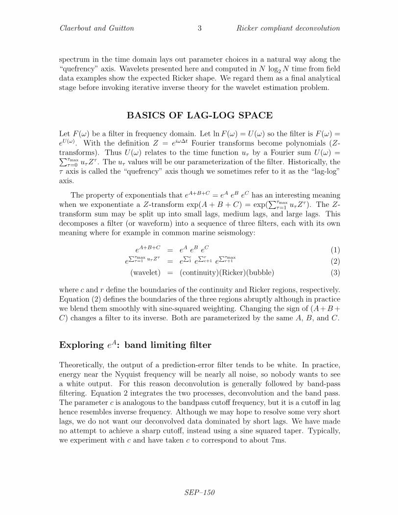
A long-standing assumption in reflection seismology is that seismic sources are min-imum phase (Robinson and Treitel, 1964). This means the source wavelet and itsinverse (the decon filter) are both causal. The decon filter is derived from the dataspectrum. Its inverse should be the source wavelet. These assumptions lead to thenon-plausible source waveforms in Figure 1. We should be seeing something closer tothe symmetrical Ricker wavelet (Ricker, 1953): let Z = eiωdt where dt is the two waytravel time from the gun (or the receiver) to the surface and back. Since the surfacereflection coefficient is -1, the frequency response at the gun is 1 − Z and at thehydrophone is also 1−Z making the composite response 1− 2Z +Z2. Therefore, theRicker wavelet results from a water-surface ghost at the marine gun convolved withanother at the hydrophone (Lindsey, 1960). In all four of the deep-marine regionswe tested and show in Figure 1, the minimum-phase source wavelets estimated withthe Kolmogoroff method (see below) have the expected three lobes, but they are notsymmetric. The first lobe is more than double the third. This is a long-standingissue in seismic processing (Levy and Oldenburg, 1982) and many methods based, forinstance, on homomorphic transformations (Jin and Rogers, 1983), frequency domainfiltering (Ghosh, 2000), higher order statistics (Sacchi and Ulrych, 2000) or stochasticmethods (Velis, 2008) have been proposed to handle non minimum-phase wavelets.

In the conflict between the Ricker idea and the minimum-phase idea we take ithere that the Ricker idea is closer to the truth (Rice, 1962). The main contributionof this paper is a method for finding phase that respects Ricker symmetry. The newtime origin is at the center of the Ricker wavelet. With the new seismic wavelet,seismogram polarity will be seen more apparent. A byproduct of this approach is adebubble process giving results of outstanding clarity.

Our proposed method is a simple addition to the Kolmogoroff method in the lag-log domain (also known as the “cepstrum”). Parameterizing the logarithm of the

SEP–150

Claerbout and Guitton 2 Ricker compliant deconvolution

Figure 1: Estimated shot wavelets from four deep-marine regions when the minimum-phase assumption is made. They are not time symmetric about the middle lobe. Toptwo wavelets are from 4 ms data and the bottom two from 2 ms data. These results arebased on data corrected for divergence. Spectra were averaged over many hundredsof inner-offset seismograms. These spectra were not smoothed. [NR]

SEP–150

Claerbout and Guitton 3 Ricker compliant deconvolution

spectrum in the time domain lays out parameter choices in a natural way along the“quefrency” axis. Wavelets presented here and computed in N log2 N time from fielddata examples show the expected Ricker shape. We regard them as a final analyticalstage before invoking iterative inverse theory for the wavelet estimation problem.

BASICS OF LAG-LOG SPACE

Let F (ω) be a filter in frequency domain. Let ln F (ω) = U(ω) so the filter is F (ω) =eU(ω). With the definition Z = eiω∆t Fourier transforms become polynomials (Z-transforms). Thus U(ω) relates to the time function uτ by a Fourier sum U(ω) =∑τmax

τ=0 uτZτ . The uτ values will be our parameterization of the filter. Historically, the

τ axis is called the “quefrency” axis though we sometimes refer to it as the “lag-log”axis.

The property of exponentials that eA+B+C = eA eB eC has an interesting meaningwhen we exponentiate a Z-transform exp(A + B + C) = exp(

∑τmax

τ=1 uτZτ ). The Z-

transform sum may be split up into small lags, medium lags, and large lags. Thisdecomposes a filter (or waveform) into a sequence of three filters, each with its ownmeaning where for example in common marine seismology:

eA+B+C = eA eB eC (1)

ePτmax

τ=1 uτ Zτ

= ePc

1 ePr

c+1 ePτmax

r+1 (2)

(wavelet) = (continuity)(Ricker)(bubble) (3)

where c and r define the boundaries of the continuity and Ricker regions, respectively.Equation (2) defines the boundaries of the three regions abruptly although in practicewe blend them smoothly with sine-squared weighting. Changing the sign of (A+B +C) changes a filter to its inverse. Both are parameterized by the same A, B, and C.

Exploring eA: band limiting filter

Theoretically, the output of a prediction-error filter tends to be white. In practice,energy near the Nyquist frequency will be nearly all noise, so nobody wants to seea white output. For this reason deconvolution is generally followed by band-passfiltering. Equation 2 integrates the two processes, deconvolution and the band pass.The parameter c is analogous to the bandpass cutoff frequency, but it is a cutoff in laghence resembles inverse frequency. Although we may hope to resolve some very shortlags, we do not want our deconvolved data dominated by short lags. We have madeno attempt to achieve a sharp cutoff, instead using a sine squared taper. Typically,we experiment with c and have taken c to correspond to about 7ms.

SEP–150

Claerbout and Guitton 4 Ricker compliant deconvolution

Exploring eC: debubbling filter

We may specify uτ from prior knowledge, or from knowledge gained from variouskinds of data averaging, or from some mixture of the two. Commonly we begin fromKolmogoroff spectral factorization (next section) giving us all the uτ . We may designa filter eA+B+C by over-riding Kolmogoroff with A = 0 and B = 0. Such a filter woulddo nothing to its inputs at small and intermediate lags but would affect longer lags.To see what happens, consider the filter eC = 1 + C + C2/2! + · · · ≈ 1 + C. Examineits leading coefficients. They are (1, 0, 0, · · · , 0, ur+1, ur+2, ur+3, · · · ). Figure 2 showsthe application of such a filter with r = 15. This operation on the data is called“debubbling”. Debubbling in this manner seems to leave first arrivals untouched.The 15 interval gap on 4 ms data is 60 ms, a number half way between the “end ofthe ghosts” and the “onset of the bubbles”. This result may be described as “textbookquality” (meaning it is the best we have ever produced).

Figure 2: Gulf of Mexico data before (a) and after debubble (b). This process pre-serves the wave onset while it lifts off the bubbles. Here the effect of the process isvisible nearly everywhere after 2.4 sec, but also visible around 1.85 sec. On blinkingdisplays it is easy to see bubble removed nearly everywhere. [NR]

Before we go on to attack the middle-lag terms we review the starting point,Kolmogoroff spectral factorization.

SEP–150

Claerbout and Guitton 5 Ricker compliant deconvolution

Kolmogoroff spectral factorization

When a time function such as bt vanishes at all negative time lags it is said to becausal. Its Z transform is B(Z) = b0 + b1Z + b2Z

2 + b3Z3 + · · · . Observe that

B(Z)2 is also causal because it has no negative powers of Z, alternately, because theconvolution of a causal with a causal is causal. Likewise eB is causal because it is asum of causals.

eB = 1 + B + B2/2! + B3/3! + · · · (4)

Happily, this infinite series always converges because of the strong influence of thedenominator factorials. The time-domain coefficients for eB could be computed thehard way, putting polynomials into power series, or eB may be computed by Fouriertransforms. To do so, we would evaluate B(Z) for many real ω, and then invoke aninverse Fourier transform program to uncover the time-domain coefficients.

Let r = r(ω), φ = φ(ω), and Zτ = eiωτ . Let us investigate the consequence ofexponentiating a causal filter.

|r|eiφ = eln |r|+iφ = eP

τ bτ Zτ

(5)

Notice a pair of filters, both causal and inverse to each other.

|r|eiφ = e+P

τ bτ Zτ

(6)

|r|−1e−iφ = e−P

τ bτ Zτ

(7)

A filter from any such pair is said to be “minimum phase”. Many filters are notminimum phase because they have no causal inverse. For example the delay filterZ. It’s inverse, Z−1 is not causal. Such filters do not relate to a causal complexlogarithm. If they have a logarithm, it must be non causal.

Given a spectrum r(ω) we can construct a minimum-phase filter with that spec-trum. Since r(ω) is a real even function of ω, the same may be said of its logarithm.Let the inverse Fourier transform of ln |r(ω)| be eτ , where eτ is a real even functionof time. Imagine a real odd function of time oτ .

|r|eiφ = eln |r|+iφ = eP

τ (eτ+oτ )Zτ

(8)

The phase φ(ω) transforms to oτ . We can assert causality by choosing oτ so thateτ + oτ = 0 for all negative τ . This defines oτ at negative τ . Since oτ is odd, wealso know its values at positive lags. This creates a causal exponent which createsa causal minimum-phase filter with the specified spectrum. Therefore the causalminimum-phase filter is simply obtained by multiplying eτ by a step function ofheight 2 to preserve the real part. This computation is called Kolmogoroff spectralfactoring. The word “factoring” enters because in applications one begins with anenergy spectrum |r|2 and factors it into an reiφ times its conjugate (time reverse).

SEP–150

Claerbout and Guitton 6 Ricker compliant deconvolution

Ricker compliant decon

Start with the bτ resulting from a Kolmogoroff factorization described above. Splitit into even and odd parts, uodd

τ = (bτ − b−τ )/2 and uevenτ = (bτ + b−τ )/2 whose sum

is bτ . The even part Fourier transforms to the logarithm of the amplitude spectrum(i.e., equation 8). The odd part Fourier transforms to the phase spectrum. Herewe monkey with the phase while not changing the amplitude. We simply taper uodd

τ

towards zero for small lags. Figure 3a shows an illustration of an odd function togetherwith the weighting function going smoothly to zero at negative lags in Figure 3b. Theparameter τa controls the amount of anticausality in the wavelet. Figure 4 examinesthe consequences of various numerical choices of τa for the data in Figure 2a. Inpractice, the cepstrum of all traces is averaged before applying the decon. As weincrease the anticausality, the time function of the wavelet eB increases in symmetrynear t = 0. Our favored choice is τa = 64 ms: it is larger than the Ricker width,about 20 ms, but not as large as the bubble delay, about 150 ms.

⌧

⌧

uodd

⌧(a)$

(b)$ w(⌧)1$

⌧a⌧a'$

Figure 3: The odd part of bτ (a) and the weighting function (b). The parameter τa

determines the amount of anticausality in the wavelet. [NR]

Removing all the phase of any wavelet makes it symmetric in time. Any deconvo-lution filter can be made Ricker-compliant simply by transforming its phase function

SEP–150

Claerbout and Guitton 7 Ricker compliant deconvolution

Figure 4: Gulf of Mexico ∆t = 4 ms: Increasing the anticausality τa in Rickercompliant decon. Too much (τa > 128 ms) causes half the bubble to appear beforethe shot. τa = 0 ms corresponds to the minimum-phase wavelet. In this manuscript,our favored choice is τa = 64 ms. [NR]

SEP–150

Claerbout and Guitton 8 Ricker compliant deconvolution

from frequency to time lag. Suppressing the phase only near zero lag makes thewavelet symmetric only near zero lag (Ricker like).

The next section presents Ricker deconvolutions and debubbling examples on threefield datasets. For all these examples, we use portions of the near-offset sectionscompensated for spherical divergence and attenuation (applying a t2 correction). Allthese results demonstrate the effectiveness of the proposed method for estimatingRicker-like, zero-phase wavelets as well as debubbling seismic data.

RICKER DECONVOLUTION AND DEBUBBLINGRESULTS

We first start by presenting results of the debubbling process on a dataset fromoffshore Baja California (also called “Cabo” in this manuscript) shown in Figure 5a.Debubbling (Figure 5b) is very effective as the bubbles are lifted off everywhere inthe section (the first bubble arrives 150 ms after the main spike.)

Figure 5: Cabo data before (a) and after debubble (b). This process preserves thewave onset while it lifts off the bubbles. [NR]

Then, the Ricker deconvolution applied to the Gulf of Mexico dataset of Figure2b is shown in Figure 6a with c = 0 ms and in Figure 6b with c = 10 ms. Increasingc acts as a bandpass filter by attenuating high-frequencies. The same filtering effectis seen with the Cabo dataset in Figure 7b. Notice in both Figures 6 and 7 howthe deconvolution is able to remove the Ricker-like behavior of the main reflections.

SEP–150

Claerbout and Guitton 9 Ricker compliant deconvolution

Figure 6: Ricker deconvolution results applied to the Gulf of Mexico dataset in Figure2 for (a) c = 0 ms and (b) c = 10 ms. [NR]

Figure 7: Ricker deconvolution results applied to the Cabo dataset for (a) c = 0 msand (b) c = 10 ms. [NR]

SEP–150

Claerbout and Guitton 10 Ricker compliant deconvolution

Figure 8 displays the different waveforms extracted from the Gulf of Mexico andBaja California datasets. Figures 8a and 8b show the Ricker wavelets (including thebubbles) extracted with our process. Figures 8c and 8d show the bubbles only (eC inequation 2). The bubbles, deconvolved from the ghosts, show uniform polarity.

Figure 8: Bottom row shows the seismic source function after the ghosts have beenremoved (bubble only), top row before. Removing the ghosts reveals the uniformpolarity of the bubbles. [NR]

Finally, we apply the Ricker deconvolution to a near-offset section from offshoreAustralia. Figure 9a shows the input data, sampled at 2 ms. Figure 9b shows thedeconvolution result (using our default c = 10 ms). The Ricker wavelet and bubblesextracted are shown in Figure 10. Note how weak the bubbles are in this case, showingthat the gun array was very well tuned (contrary to the other two field data examples,because the bubbles are so small, we decided against showing the debubbled section).

CONCLUSION

The proposed analytical method, a simple addition to the Kolmogoroff factorization,works well on the three data sets tested. Simply stated, phase, normally a function

SEP–150

Claerbout and Guitton 11 Ricker compliant deconvolution

Figure 9: Dataset from offshore Australia (a) before and (b) after Ricker deconvolu-tion. [NR]

Figure 10: Waveforms extracted from the Australia datasets: (a) effective Rickerwavelet and (b) estimated bubbles. In this case, the bubbles are very weak. [NR]

SEP–150

Claerbout and Guitton 12 Ricker compliant deconvolution

of frequency, is brought into the time lag domain and altered (suppressed) near zerolag. Additionally, it might provide an initialization and provide a regularization thatshould be helpful in fitting more complicated data models.

REFERENCES

Ghosh, S., 2000, Deconvolving the ghost effect of the water surface in marine seismics:Geophysics, 65, 1831–1836.

Jin, D. and J. Rogers, 1983, Homomorphic deconvolution: Geophysics, 48, 1014–1016.

Levy, S. and D. Oldenburg, 1982, The deconvolution of phase-shifted wavelets: Geo-physics, 47, 1285–1294.

Lindsey, J., 1960, Elimination of seismic ghost reflections by means of a linear filter:Geophysics, 25, 130–140.

Rice, R., 1962, Inverse convolution filters: Geophysics, 27, 4–18.Ricker, N., 1953, The form and laws of propagation of seismic wavelets: Geophysics,

18, 10–40.Robinson, E. and S. Treitel, 1964, Principles of digital filtering: Geophysics, 29,

395–404.Sacchi, M. and T. Ulrych, 2000, Nonminimum-phase wavelet estimation using higher

order statistics: The Leading Edge, 19, 80–83.Velis, D., 2008, Stochastic sparse-spike deconvolution: Geophysics, 73, R1–R9.

SEP–150